EP1526468A2 - Procédé de simulation d'un matériau viscoélastique - Google Patents
Procédé de simulation d'un matériau viscoélastique Download PDFInfo
- Publication number
- EP1526468A2 EP1526468A2 EP04017402A EP04017402A EP1526468A2 EP 1526468 A2 EP1526468 A2 EP 1526468A2 EP 04017402 A EP04017402 A EP 04017402A EP 04017402 A EP04017402 A EP 04017402A EP 1526468 A2 EP1526468 A2 EP 1526468A2
- Authority
- EP
- European Patent Office
- Prior art keywords
- model
- filler
- viscoelastic material
- simulating
- matrix
- Prior art date
- Legal status (The legal status is an assumption and is not a legal conclusion. Google has not performed a legal analysis and makes no representation as to the accuracy of the status listed.)
- Granted
Links
- XFHMIJDAGQLVAF-UHFFFAOYSA-N C=CCCC1COCC1 Chemical compound C=CCCC1COCC1 XFHMIJDAGQLVAF-UHFFFAOYSA-N 0.000 description 1
Images


Classifications
-
- G—PHYSICS
- G01—MEASURING; TESTING
- G01N—INVESTIGATING OR ANALYSING MATERIALS BY DETERMINING THEIR CHEMICAL OR PHYSICAL PROPERTIES
- G01N19/00—Investigating materials by mechanical methods
-
- G—PHYSICS
- G06—COMPUTING; CALCULATING OR COUNTING
- G06F—ELECTRIC DIGITAL DATA PROCESSING
- G06F30/00—Computer-aided design [CAD]
- G06F30/20—Design optimisation, verification or simulation
- G06F30/23—Design optimisation, verification or simulation using finite element methods [FEM] or finite difference methods [FDM]
-
- G—PHYSICS
- G01—MEASURING; TESTING
- G01N—INVESTIGATING OR ANALYSING MATERIALS BY DETERMINING THEIR CHEMICAL OR PHYSICAL PROPERTIES
- G01N11/00—Investigating flow properties of materials, e.g. viscosity, plasticity; Analysing materials by determining flow properties
-
- G—PHYSICS
- G06—COMPUTING; CALCULATING OR COUNTING
- G06F—ELECTRIC DIGITAL DATA PROCESSING
- G06F2111/00—Details relating to CAD techniques
- G06F2111/10—Numerical modelling
Definitions
- the present invention relates to a method of simulating useful in analyzing, with good accuracy, deformation and the like of the viscoelastic material.
- the viscoelastic material as represented by rubber is widely used in for example, tires and industrial goods such as sporting goods.
- the viscoelastic material deforms greatly when subjected to load, and restores to the original state when the load is completely removed or is unloaded.
- the viscoelastic material has a non-linear elastic behavior under static load and a rate-dependent or viscoelastic behavior with hysteresis under cyclic loading.
- a simulation of for example, deformation process of the viscoelastic material is carried out using a computer.
- a conventional simulation method of the viscoelastic material is disclosed in Japanese Laid-Open Patent Publication No. 2002-365205.
- the above mentioned publication focuses on the fact that the viscoelastic material shows a different modulus of longitudinal elasticity in accordance with strain velocity. More specifically, strain, strain velocity and stress produced in the relevant viscoelastic material are measured under a measuring condition assuming, in advance, the actual usage state of the viscoelastic material. Thus, the corresponding relationship between the modulus of longitudinal elasticity and the strain velocity is obtained. With respect to a viscoelastic material model serving as an analyzing object, a predetermined strain velocity is given and the modulus of longitudinal elasticity is appropriately calculated from the above corresponding relationship to perform the deformation calculation.
- the simulation method of the viscoelastic material is described in for example, the following article.
- the above mentioned article is premised on the molecular chain network model theory in which the viscoelastic material has a network structure as a microscopic structure.
- the network structure of the viscoelastic material "a" includes a plurality of molecular chains c linked at a linking point b.
- the linking point b includes a chemical linking point between the molecules such as for example, a chemical cross-linking point.
- One molecular chain c is configured by a plurality of segments e.
- One segment e is the smallest constitutional unit for repetition.
- one segment e is configured by joining a plurality of monomers f in which carbon atoms are linked by covalent bonding. Carbon atoms each freely rotates with respect to each other around a bond axis between the carbons. Thus, the segment e can be bent, as a whole, into various shapes.
- Aruuda et al. also proposes an eight chain rubber elasticity model.
- this model is defined the macroscopic structure of the viscoelastic material as a cubic network structure body h in which the microscopic eight chain rubber elasticity models g are collected.
- the molecular chain c extends from one linking point b1 placed at the center of the cube to each of the eight linking point b2 at each apex of the cube, as shown enlarged on the right side of Fig. 6.
- the viscoelastic material is defined as a super-elastic body in which volume change barely occurs and in which restoration to the original shape occurs after the load is removed.
- the super-elastic body is, as expressed in the following equation (1), defined as a substance having a strain energy function W that is differentiated by a component Eij of Green strain to produce a conjugate Kirchhoff stress Sij.
- the strain energy function shows the presence of potential energy stored when the viscoelastic material deforms. Therefore, the relationship between the stress and the strain of the super-elastic body is obtained from a differential slope of the strain energy function W.
- S ij ⁇ W ⁇ E ij
- filler such as carbon black and silica
- filler such as carbon black and silica
- the present invention aims to propose a method of simulating the viscoelastic material useful in simulating, with good accuracy, the deforming state of modeling of the viscoelastic material on the basis of including a step of dividing the viscoelastic material into a finite number of elements, and a step of dividing at least one filler into a finite number of elements to form a filler model.
- the present invention proposes a method of simulating the deformation of a viscoelastic material in which filler is blended to a matrix made of rubber or resin, the method including the steps of dividing the viscoelastic material into a finite number of elements to form a viscoelastic material model, a step of performing deformation calculation of the viscoelastic material model based on a predetermined condition, and a step of acquiring a necessary physical amount from the deformation calculation, where the step of dividing the viscoelastic material into a finite number of elements includes a step of dividing at least one filler into a finite number of elements to form a filler model, and a step of dividing the matrix into a finite number of elements to form a matrix model.
- the present invention includes a step of dividing the filler to form a filler model. Therefore, the effect of the filler can be taken into consideration to the result of the deformation calculation of the viscoelastic material model.
- the step of dividing the viscoelastic material into a finite number of elements further desirably includes a step of arranging an interface model having a viscoelastic property different from the matrix model between the matrix model and the filler model.
- the interface model may have a viscoelastic property softer than the matrix model, a viscoelastic property harder than the matrix model, and a viscoelastic property in which a hysteresis loss is greater than the matrix model.
- a relationship between the stress and the strain is desirably defined to simulate the energy loss of the matrix rubber.
- the filler model desirably includes at least two filler models of a first filler model and a second filler model arranged at a distance from each other.
- the inter-filler model having an inter-filler attractive force that changes with the distance is arranged between the first filler model and the second filler model. This is useful in taking the interaction between fillers into consideration in the deformation calculation of the viscoelastic material model.
- the inter-filler attractive force is desirably set based on a function for a parabolic curve including a gradually increasing region that smoothly increases and reaches a peak with an increase in the distance between the first filler model and the second filler model, and a gradually decreasing region that smoothly decreases and reaches zero at a predetermined characteristic length with a further increase in the distance. Further, a step of linearly decreasing the inter-filler attractive force from a value of start of unloading to zero in the unloaded deformation from the gradually decreasing region is included to take the hysteresis loss produced between the first filler model and the second filler model into consideration in the simulation.
- Fig. 1 shows a computer apparatus 1 for carrying out a simulation method according to the present invention.
- the computer apparatus 1 includes a main unit 1a, a keyboard 1b, and a mouse 1c serving as input means, and a display 1d serving as output means.
- the main unit 1a is appropriately provided with a central processing unit (abbreviated as "a CPU"), a ROM, a working memory, a large-capacity storage device such as a magnetic disk, and drives 1a1 and 1a2 for a CD-ROM or a flexible disk.
- the large-capacity storage device stores therein processing procedures (i.e., programs) for executing a method, described later.
- An Engineering Work Station and the like are preferably used as the computer apparatus 1.
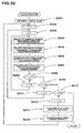
- Fig. 2 shows one example of a processing procedure of the simulation method according to the present invention.
- a viscoelastic material model is first set (step S1).
- Fig. 3 one example of the viscoelastic material model 2 serving as a microscopic structure is visually shown.
- a microscopic region of the viscoelastic material (no object on whether existent or not) to be analyzed is divided into a finite number of small elements 2a, 2b, 2c ⁇ .
- a parameter necessary for deformation calculation using a numerical analysis method is given to each element 2a, 2b, 2c ....
- the numerical analysis method includes for example, finite element method, finite volume method, calculus of finite differences, or boundary element method.
- the parameter includes for example, node coordinate value, element shape, and/or material property of each element 2a, 2b, 2c ... .
- the viscoelastic material model 2 is numerical data utilizable in the computer apparatus 1.
- the two-dimensional viscoelastic material model is shown.
- Fig. 4 shows, in detail, steps for setting the viscoelastic material model 2.
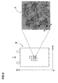
- the viscoelastic material model 2 is set by a step S11 of dividing a matrix into a finite number of elements and forming a matrix model 3, a step S12 of dividing at least one filler into a finite number of elements and forming a filler model 4, and a step S13 of forming an interface model 5 having a viscoelastic property different from the matrix model 3.
- the viscoelastic material model 2 shown is thus configured with the matrix model 3 in which the matrix made of rubber or resin is modeled, the filler model 4 (white part), distributed and blended in the matrix model 3, and in which the filler is modeled, and the interface model 5 (darkish part) interposed between the matrix model 3 and the filler model 4 to form interfaces between the models.
- the matrix model 3 is the darkest part.
- the matrix model 3 constitutes a main part of the viscoelastic material model 2 and is divided into triangular or quadrilateral elements in this example.
- a relationship between the stress and the strain expressed in for example, the following equation (3) for the material property is given to each element of the matrix model 3.
- C R n ⁇ k B ⁇ T ( n : number of molecular chains per unit volume; k B : Boltzmann constant; T: absolute temperature)
- Equation (3) A derivation process of equation (3) will now be briefly explained.
- the viscoelastic material such as rubber has very small volume change during deformation, and can be ignored in the calculation.
- the calculation can be performed having a density of the viscoelastic material as a constant. Therefore, the Kirchhoff stress S ij can be expressed as equation (4).
- E ij is a component of Green strain
- p is a hydrostatic pressure
- Xi is a position of an arbitrary object point P in a state C0 where stress and strain are
- x j is a position of the object point P in a deformed state C.
- equation (6) can be obtained from equation (4).
- equation (11) the velocity form display of equation (7) is expressed as equation (11).
- the Jaumann velocity of Cauchy stress shown in equation (11) can be replaced by the Jaumann velocity of Kirchhoff stress. Further, by replacing the deformation velocity tensor D with the strain velocity tensor, the constitutive equation of the velocity form display of a non-compressible viscoelastic material is obtained as equation (3).
- the inventor et al. attempted various improvements on the premise of the model of Aruuda et al. As state above, the viscoelastic material tolerates great strain reaching to several hundred % by stretching a long molecular chain c intricately intertwined with each other. The inventor et al. hypothesized that a portion intertwined with respect to each other of the molecular chain c of the viscoelastic material may come loose and disappear (reduction in the number of linking point b), or that by removing the load, intertwining may again be produced (increase in the number of linking point b) during the loaded deformation process.
- each molecular chain c1 to c4 stretches and the linking point b is subjected to great strain and tends to break (disappear).
- the two molecular chains c1 and c2 act as one long molecular chain c5.
- the molecular chains c3 and c4 also act in the same way. Such phenomenon sequentially occurs as the loaded deformation of the rubber material proceeds and large amount of energy loss tends to occur.
- an average segment number N per one molecular chain c is defined as a variable parameter that differs between the loaded deformation and the unloaded deformation.
- the loaded deformation refers to increase in strain of the matrix model 3 during a minimal time
- the unloaded deformation refers to decrease in strain.
- the macroscopic three-dimensional network structure body h of Fig. 6 is again referred to in view of the above points.
- the network structure body h is a body in which k number of eight chain rubber elasticity model are each bonded in the directions of the axis, the height, and the depth. It is to be noted that k is a sufficiently big number.
- the total number of linking point b included in the relevant network structure body h is referred to as "binding number".
- the binding number m may be expressed by n, as equation (16).
- n n/4
- the binding number m of the molecular chain of the rubber needs to be changed to have the average segment number N as the variable parameter.
- the energy loss of the matrix model 3 can be simulated.
- the average segment number N is determined by various methods. For instance, the average segment number N can be increased based on the parameter related to strain during the loaded deformation.
- the parameter related to strain is not particularly limited and may be for example, strain, strain velocity, or primary invariable quantity I 1 of strain.
- the average segment number N is defined by the following equation (19). This equation shows that the average segment number N is a function of the primary invariable quantity I 1 (more specifically, a parameter ⁇ c square root thereof) of strain in each element of the relevant matrix model 3.
- N( ⁇ c) A + B• ⁇ c + C• ⁇ c 2 + D• ⁇ c 3 + E• ⁇ c 4
- ⁇ c I 1 3
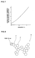
- the average segment number N in each strain is derived so as to comply with the curve during when load is loaded.
- a relationship between the average segment number N and the parameter ⁇ c during loaded deformation of each element of the matrix model 3 is shown.
- ⁇ c a parameter relating to strain
- the average segment number N is also gradually increased.
- the upper limit of parameter ⁇ c is 2.5.
- the parameter ⁇ c of each element of the matrix model 3 is calculated on a steady basis.
- the calculated ⁇ c is substituted to equation (19), and the average segment number N during the relevant strain state of the relevant element is calculated.
- the value of the average segment number N during the unloaded deformation of the matrix model 3 is constant.
- the filler model 4 in which a carbon black is modeled is shown. It is to be noted that the filler is not limited to carbon black and may be for example, silica and the like.
- the physical shape of the filler model 4 is set based on the shape of the carbon black filled in the actual rubber imaged with an electronic microscope.
- Fig. 8 shows a secondary particle of the carbon black 6.
- the secondary particle has, more specifically, a structure in which a plurality of spherical primary particles 7 each consisting of carbon atom having a diameter of approximately 10 nm is irregularly bonded three-dimensionally.
- the carbon black 6 has hardness (modulus of longitudinal elasticity) several hundred times harder than the matrix rubber.
- the filler model 4 is defined as an elastic body instead of a viscoelastic body in the present embodiment. Therefore, the filler model 4 has a modulus of longitudinal elasticity as the material property, and the stress and the strain are proportional in the deformation calculation.
- the number of filler model 4 is appropriately set based on the filler blending amount of the viscoelastic material of the analyzing object.
- the interface model 5 is provided between the matrix model 3 and the filler model 4.
- the interface model 5 is not necessarily limited to continuously surround the filler model 4, but preferably, surrounds the filler model 4 throughout the entire range.
- the interface model 5 has a small thickness.
- the thickness t of the interface model 5 is for example, between 1 and 20 nm, and more preferably, between 5 to 10 nm.
- the physical structure having an interface layer having such physical thickness on the interfaces of the filler and the rubber matrix is not actually recognized.
- various phenomenons for causing energy loss such as slippage and friction are recognized on the interfaces of the filler and the matrix rubber.
- the interface model is defined as the viscoelastic material in the calculation in the simulation. Therefore, similar to matrix model 3, the relationship between the stress and the strain expressed in equation (3) is defined for the interface model 5.
- the interface model 5 has a viscoelastic property different from the matrix model 3.
- the interface model 5 of the present embodiment has a viscoelastic property softer than the matrix model 3. Therefore, when the same stress acts on the interface model 5 and the matrix model 3, the strain of the interface model 5 becomes greater than the strain of the matrix model 3. Further, the interface model 5 has a viscoelastic property in which the hysteresis loss (energy loss produced per 1 cycle of strain) is greater than the matrix model 3. This is carried out by for example, adjusting the parameter of equation (19) for calculating the average segment number N applied to equation (3).
- step S3 a deformation condition of the viscoelastic material model 2 is set.
- the viscoelastic material model 2 is deformed under a condition of uniaxial tension (plane strain state). Therefore, the viscoelastic material model 2 does not have strain in the direction of the Z axis of Fig. 3.
- the deformation condition includes strain velocity and maximum strain of when the viscoelastic material model 2 deforms.
- the deformation calculation may be carried out on one microscopic piece of viscoelastic material model 2 shown in Fig. 2, but is preferably carried out, as shown in Fig. 9, using a viscoelastic material entire model M in which the microscopic structure of the viscoelastic material model 2 (viscoelastic material model 2 shown in Fig. 3) is periodically repeated in the vertical and the horizontal direction.
- a homogenizing method is desirably used.
- the extent of repetition of the microscopic structure is very close.
- the homogenizing method as shown in Fig. 9, two independent variables of macroscopic scales x 1 , x 2 representing the viscoelastic material entire model M and the microscopic scales y 1 , y 2 representing the above mentioned microscopic structure are used.
- the respective independent variable in different scales of the microscopic scales y 1 , y 2 and the macroscopic scales x 1 , x 2 are asymptotically developed.
- an average dynamic response of the viscoelastic material entire model M of a certain size periodically including a model structure of the microscopic structure shown in Fig. 3 can be obtained.
- the asymptotically developing homogenizing method is a method already established in the numerical calculation method. The method is described in detail in for example, the following article.
- the length of one side of the viscoelastic material model 2 is 300 nm ⁇ 300 nm, and the viscoelastic material entire model M shown in Fig. 9 has an oblong shape of 2mm ⁇ 2mm.
- a constant strain velocity is applied to the microscopic structure of Fig. 3 so as to cause a uniform uniaxial tensile strain E 2 (strain velocity thereof is 1.0 ⁇ 10 -5 /s).
- strain velocity thereof is 1.0 ⁇ 10 -5 /s.
- the deformation calculation (simulation) using the set model and condition is performed (step S3).
- Fig. 10 one example of a specific procedure of the deformation calculation is shown.
- data is first input to the computer apparatus 1 (step S31).
- the input data includes for example, numerical data for configuring the viscoelastic material model 2, and a variety of pre-set boundary conditions.
- a rigid matrix of each element is then formed (step S32), and thereafter, the rigid matrix of the entire structure is assembled (step S33).
- a known node displacement and node force are adopted to the rigid matrix of the entire structure (step S34), and an analysis of the rigidity formula is carried out.
- the unknown node displacement is determined (step S35) and physical quantity such as strain, stress, and principal stress of each element are calculated and output (step S36, S37).
- step S38 a determination is made whether or not to finish the calculation, and if the calculation is not to be finished, steps after step S32 is repeated.
- Equation (20) is used for the element equation based on the principal of virtual work.
- the deformation calculation may be carried out using an engineering system analyzing application software (e.g., LS-DYNA and the like, developed and improved in Livermore Software Technology Corporation (US)) using the finite element method.
- application software e.g., LS-DYNA and the like, developed and improved in Livermore Software Technology Corporation (US)
- the average segment number N is calculated for each strain state, as mentioned above, and such value is substituted to equation (3) and the calculation is sequentially carried out.
- the three-dimensional eight chain rubber elasticity model of Aruuda et al. is used in the viscoelastic material model 2 and the viscoelastic material entire model M without changing in the direction of thickness (direction of Z axis in Fig. 3).
- strain, stress and the like of the element are calculated for every constant time increment, and such values are sequentially recorded (step S37).
- the necessary physical quantity is taken out therefrom and is used for analysis (step S4 of Fig. 2).
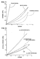
- Fig. 11 the results of the deformation calculation independently carried out on the matrix model 3, the filler model 4, and the interface model 5 are shown.
- the filler model 4 shows the highest elasticity, and no energy loss occurs.
- the interface model 5 shows a softer viscoelastic property and a greater energy loss (loop surface area defined by the curves) than the matrix model 3.
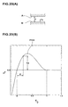
- Fig. 12 a relationship between the actual stress and the strain of the viscoelastic material entire model M is shown.
- the curve La shows the result of when the interface model 5 is made softer than the matrix model 3.
- a non-linear first curve La1 is obtained during the loaded deformation.
- a second curve La2 different from the first curve La1 is obtained during the unloaded deformation.
- the second curve La2 is softer (lower elasticity) than the first curve La1, and a hysteresis loop is produced.
- the energy loss in one cycle of tensile deformation can be obtained.
- the shapes of the first and the second curves La1, La2 can be set to a variety of shapes by appropriately changing the coefficients A to E in equation (19). Therefore, by setting the coefficients A to E in accordance with the viscoelastic material to be analyzed, for example, the energy loss and the like can be accurately studied for each material. This is very useful in improving the performance of industrial goods such as tires, and golf balls that uses the viscoelastic material as the main part.
- Fig. 12 the calculation result of the model in which the material property same as that of the matrix model 3 is given to the interface model 5, that is, the model not taking the interface into consideration, is shown as a curve Lb with an alternate long and short dash line.
- the slope of the stress-strain curve is raised compared to the curve La.
- great energy loss is not likely to occur at the interface as with the interface model 5, the energy loss of the entire model is small.
- the calculation result of the model having a viscoelastic property opposite of the curve La is shown as curve Lc with a chained line.
- the interface model 5 has a viscoelastic property harder than the matrix model 3 as shown in Fig. 13. It is recognized that the curve Lc has high elasticity, as expected.
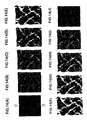
- Fig. 14 the progressing process from the deformed state to the restored state of one microscopic structure (unit cell) in the simulation of tensile deformation of the viscoelastic material model 2 (curve La) is visually shown. It is to be noted that the processes are not continuous in the deformation calculation and an appropriate time interval is provided.
- Figs. 14(A) to 14(E) show the loaded deformation and Figs. 14(F) to 14(J) show the unloaded deformation.
- the level of stress is represented with change in color. The region where the color is changing white shows the region of great strain. This result accurately shows that great strain is concentrated between the interfaces of the filler model 4 or between the filler models 4, 4. Particularly, it can be seen that great strain occurs in a region where the distance between the filler models 4, 4 is small.
- Fig. 15(A) corresponds to the curve Lb of Fig. 12 that does not take interface into consideration
- Fig. 15(B) corresponds to the curve La that takes interface into consideration.
- the figure shows that greater strain occurs in a region where the color is light.
- Fig. 15(A) where the interface is not taken into consideration strain occurs entirely and extensively and mildly
- Fig. 15(B) where the interface is taken into consideration the great strain is concentrated at the peripheral (or near the interface) of the filler model 4.
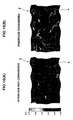
- Fig. 16 the energy loss of one cycle of strain for each element, and the sizes thereof are shown with a color.
- the figure shows that great energy loss occurs more in one cycle in a region where the color is light.
- the shape of the model is shown with the maximum deformed shape of Fig. 15.
- Fig. 16(A) corresponds to curve Lb of Fig. 12
- Fig. 16(B) corresponds to curve La of Fig. 12.
- Fig. 16(B) where the interface is taken into consideration, it can be seen that great energy loss is concentrated at the interface of the filler model 4.
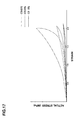
- rubber blended with carbon black serves as a viscoelastic material for the object to be analyzed.
- Fig. 17 stress-strain curves of rubber material with different blending amount CB of carbon black are shown.
- the rubber material having large blending amount CB of carbon black has large surface area of the hysteresis loop.
- the rubber material having large blending amount of filler tends to have large energy loss.
- One cause of this is thought to be due to interaction acting between the filler particles. That is, an inter-filler attractive force similar to van der Waals force is believed to act between two filler particles approaching at a level of a few nano in the rubber matrix. This theory is presently dominant.
- an attempt is made to consider the inter-filler attractive force in the deformation calculation.
- the viscoelastic material model 2 of this example includes the matrix model 3 in which the matrix rubber is divided, a filler model 4A, 4B (collectively referred to as simply "filler model 4") in which at least two filler particles arranged with a spacing in between is divided, and an inter-filler model 10 arranged between the two filler models 4A, 4B and has an inter-filler attractive force that changes in accordance with the distance between the filler models 4A, 4B.
- This viscoelastic material model does not include the interface model.
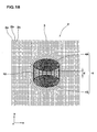
- the microscopic structure (unit cell) of the viscoelastic material model 2 is formed so as to be symmetrical with respect to each center line of the x-axis and the y-axis.
- the matrix model 3 and the filler model 4 are defined the same way as in the above mentioned embodiment.
- the two filler models 4 each have an elliptical shape and are of the same size.
- the filler model 4A, 4B are separated by a smallest distance d(d ⁇ 0) and does not contact each other.
- the initial smallest distance d between the filler model 4A and the filler model 4B is desirably selected within a range of, for example, about 1 to 3 nm. It is to be noted that such value may be changed in accordance with the position of the filler model 4, the conditions of the simulation and the like.
- the inter-filler model 10 is arranged between the filler model 4A and the filler model 4B.
- the inter-filler model 10 overlaps the matrix model 3 in the direction of the z-axis.
- each inter-filler model 10 is a quadrilateral element.
- two nodes are shared with nodes on the outer peripheral surface of one of the filler model 4A, and the remaining two nodes are shared with nodes on the outer peripheral surface of the other filler model 4B. Therefore, in the deformation calculation, when the distance d between the two filler models 4A, 4B changes, the coordinate of each node of the inter-filler model 10 changes, thereby changing the shape (surface area) thereof.
- the inter-filler attractive force is defined by the inter-filler model 5.
- the inter-filler attractive force can be defined with reference to the following article in which an adhesive force acting on the interface when the phase II particle is debonded from a metal matrix layer is formulated.
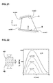
- Fig. 20(A) shows a diagram of interfaces A, B to which debonding is started, proposed by Needleman et al.
- the interfaces A, B correspond to the outer peripheral surfaces of the filler models 4A, 4B.
- Fig. 20(B) a relationship between the attractive force Tn produced between the interfaces A, B and the distance d is shown.
- the ⁇ on the horizontal axis of Fig. 20(B) is the limiting length of when the attractive force Tn becomes zero when the distance d between the interfaces A, B is increased, and this length is hereinafter referred to as a characteristic length.
- the attractive force Tn between the interfaces A, B is determined by a function for a parabolic curve including a gradually increasing region in which the attractive force smoothly increases and reaches a peak ( ⁇ max) with the increase in distance d, and a gradually decreasing region in which the attractive force smoothly decreases and reaches zero at a pre-set characteristic length with a further increase in distance d.
- This function is defined, two-dimensionally, as equation (23).
- u n ,u s are each relative displacement of the normal line and the tangent line in the interfaces A, B, and ⁇ n , ⁇ s are characteristic lengths of the normal line and the tangent line.
- the normal line n and the tangent line s are as shown in Fig. 21.
- the inter-filler attractive force is determined with the above equation (23).
- the distance d in the initial state is not equal to zero, but the inter-filler attractive force in the initial state is zero, between the filler model 4A, 4B.
- the following correction is made to the equation (23).
- a graph of Fig. 20(B) is shifted by -d along the horizontal axis (initial distance between the filler models) and is shifted by -Td (attractive force) along the vertical axis.
- This graph is expressed in equation (24). Therefore, in the simulation of the present embodiment, the inter-filler attractive force corresponding to the distance d between the filler models 4A, 4B is derived from equation (24).
- a function for determining the attractive force Tn when the initial distance do between the filler models 4A, 4B is changed to various values is shown.
- the initial distance do, and the characteristic length ⁇ are appropriately set in accordance with the condition.
- the distance d is greater than the characteristic length ⁇ , no inter-filler attractive force acts between the filler models 4A, 4B.
- the inter-filler attractive force Tn is set so as to linearly decrease from a value of start of unloading to a value of zero. For instance, if unloading of the load is started from an arbitrary point P3 on the gradually decreasing region YLb, as shown with a chained line arrow, the inter-filler attractive force Tn linearly decreases with values on a linear line connecting the relevant point P3 and the point P1 in accordance with the distance d.
- the attractive force Tn during such unloading is derived from the following equation (25).
- the inter-filler attractive force Tn exceeds the peak ⁇ max, a closed loop is formed at one cycle of loading and unloading of the load.
- the inter-filler attractive force determined by a function for such closed loop expresses the hysteresis loss produced between the first filler model and the second filler model. If the attractive force Tn does not exceed the peak ⁇ max, or is in the unloaded deformation from the gradually increasing region, the attractive force is determined through the same route as the loaded deformation.
- the inter-filler model 10 does not have its own rigidity as with the matrix model 3. In other words, the inter-filler model 10 is provided to calculate the inter-filler attractive force using the equation (24) and the equation (25). Each inter-filler model 10 is not divided in a direction traversing between the filler models 4A and 4B. Therefore, the shape of the inter-filler model 10 is simply determined by the relative position of the filler models 4A and 4B for each deformation, as mentioned above.
- the inter-filler attractive force (interaction force) per unit surface area between the filler models 4A, 4B is calculated.
- This inter-filler attractive force is, as shown in Fig. 21, replaced by a force acting on the four nodes 1 to 4.
- the inter-filler attractive force acts on the matrix model 3 sandwiched between the filler models 4A, 4B and compresses the matrix model 3.
- the deformation calculation is carried out under the same above mentioned condition using the above viscoelastic material model 2.
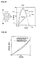
- Fig. 24 a relationship between the actual stress and the strain in the entire viscoelastic entire model periodically including the microscopic structure of Fig. 18 is shown.
- a solid line shows the result about the viscoelastic material model 2 in which the inter-filler attractive force is defined between the filler models 4A and 4B, and the broken line shows the result about the model 2 in which the attractive force is not defined.
- the simulation of the present embodiment in which the inter-filler attractive force is considered rather hard compared to a case in which the inter-filler attractive force is ignored.
- the surface area of the closed loop showing the energy loss is increased by 0.929% with respect to when the inter-filler attractive force is ignored. This corresponds to the amount of energy loss involved in the inter-filler attractive force.
- This value can be changed by setting of the parameters.
- two filler models 4A, 48 are arranged in the microscopic structure (cell unit) but by changing the density of the filler model 4 in accordance with, for example, the blending ratio of the filler in the rubber material to be analyzed, more accurate evaluation or comparison of the energy loss becomes possible.
- Fig. 25 the relationship between the attractive force produced between each inter-filler model 10 and the distance d is shown.
- the reference characters r1, r2, r3, r4 and r5 in the figure correspond to each element of the inter-filler model shown by reference characters r1, r2, r3, r4 and r5 of Fig. 19.
- Elements r1, r2 and r3 does not exceed the peak ⁇ max because the change of distance d is small.
- the attractive force Tn is considered to be the same for the loaded and the unloaded deformation.
- the initial distance d is originally large and thus no inter-filler attractive force is produced.
- the load is unloaded after the attractive force Tn has exceeded the peak, and thus is thought to have passed paths different for the loaded and the unloaded deformation, and thus the hysteresis loop is formed.
- the rubber blended with for example, carbon black serves as the viscoelastic material, and is the object of analysis.
- a potential energy is calculated as a variable representing the interaction between the fillers.
- the computer apparatus 1 shown in Fig. 1 is preferably used.
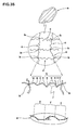
- a model setting step for setting a first filler model and a second filler model is first carried out (step S100).
- a plurality of secondary particles of carbon black 6 in the rubber polymer imaged with an electronic microscope is shown.
- the secondary particle of carbon black 6 is configured by irregularly bonding a plurality of sphere primary particles 7 three-dimensionally, as mentioned above.
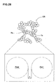
- the simulation of the present embodiment focuses on the two secondary particles 6A, 6B spaced apart from each other.
- the most approached parts of the secondary particles 6A, 6B, that is, in the example of Fig. 27, one primary particle 7a of the secondary particle 6A and one primary particle 7b of the secondary particle 6B are modeled to analyze the interaction between such approached parts. More specifically, as visually shown in Fig. 28, the primary particle 7a is modeled to a first filler model Fm1 and the primary particle 7b is modeled to a second filler model Fm2, respectively.
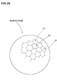
- the primary particle 7 of carbon black is a collective of carbon atoms. Therefore, the filler model Fm (simply referred to as filler model Fm when collectively referring to the first and the second filler models) in which the primary particle 7 is modeled preferably expresses a plurality of carbon atoms in the calculation.
- the filler model Fm of the present embodiment is, as visually shown in Fig. 29, shown as an assembly of a substantially hexagonal basic structure 11.
- Fig. 30(A) shows a perspective view of the visualized basic structure 11.
- the basic structure 11 is configured by superimposing a plurality of network arrays 13. In this example, for example, 3 to 5 layers of the network array 13 are stacked.
- the network array 13 includes a plurality of carbon atom model (filler-atom model) 12 and a plurality of arm models 14 for bonding the carbon atom model 12 to a hexagon in a common plane.
- the network array 13 is configured by arranging and bonding about 90 carbon atom models 12 on each apex of the regular hexagon by way of the arm model 14, as shown in Fig. 30(B). Due to the arm model 14, the relative position of each carbon atom model 12 does not change.
- the filler model Fm may be hollow, but desirably have carbon atom model 12 arrayed interiorly. This is based on a general knowledge of the present carbon particle.
- Fig. 31 shows one example of the method of setting the filler model Fm. First, as shown in Fig. 31(A), one carbon atom model 12 constituting the center of the filler model Fm is provided on a three-dimensional coordinate. Next, the basic structure 11 is arranged around the central carbon atom model 12 so as to surround the relevant carbon atom model. Here, the basic structure 11 does not need to configure a surface of a complete regular polyhedron and an open location 15 may be appropriately provided.
- the filler model Fm interiorly having multiple carbon atom models 12 is obtained, as shown in a cross sectional view of Fig. 31(C).
- the maximum diameter of the filler model Fm is desirably between, for example, 10 to 200 nm with reference to the actual shape, and the one filler model Fm preferably includes about ten thousand to one billion carbon atom models 12.
- a center of gravity coordinate of all the carbon atom models 12 included in the relevant filler model Fm is determined.
- an inherent number starting from 1 is allocated to each carbon atom model 12 in a sequential order. This number is stored in the computer apparatus 1 in relation to the coordinate and the like of the relevant carbon atom model 12.
- the first filler model Fm1 and the second filler model Fm2 are separated by a distance r.
- the distance r is desirably determined from a range of for example, about 0.1 to 1.5 nm, and in the present embodiment, 0.3 nm is set as the initial value.
- a calculation step for calculating the interaction between the filler particles acting between the first filler model Fm1 and the second filler model Fm2 is carried out using the computer apparatus (step S200).
- step S200 a calculation step for calculating the interaction between the filler particles acting between the first filler model Fm1 and the second filler model Fm2 is carried out using the computer apparatus (step S200).
- Fig. 32 one example of a specific process of the calculation step is shown.
- the distance r between the first filler model Fm1 and the second filler model Fm2 is first set to a pre-set initial value (0.3 nm in the present example) (step S201), and the variables i, j are initialized to 1 (step S202, S203).
- the variables i, j each correspond to the inherent number allocated to the carbon atom model 12. These include values i max, j max equal to the maximum value of the number of each carbon atom model 12.
- the i th number of carbon atom particle model is selected from the first filler model Fm1, and the j th number of the carbon atom model is selected from the second filler model Fm2 (step S204, S205) and the potential energy between the two models is calculated (step S206).
- the potential energy acting between the atoms spaced apart from each other can be obtained through various theoretical formulas.
- the Leonard-Jones potential energy calculation formula expressed in the following equation (26) is used.
- the Leonard-Jones potential energy calculation formula expresses the potential energy in which a close repulsive force is added to the attractive force by the van der Waals force, which formula has a relatively good accuracy and is generally widely used. However, other calculating formulas may also be used.
- the potential energy ⁇ is derived as a function of the separating distance R of the carbon atom models 12, 12. Therefore, the distance R between the i th number of carbon atom model 12 of the first filler model Fm1 and the j th number of the carbon atom model 12 of the second filler model Fm2 is calculated prior to calculating the potential energy.
- the distance R can be easily calculated using the coordinate of the i th number of carbon atom model 12 and the coordinate of the j th number of carbon atom model 12. After the distance R between the carbon atom models is calculated, the potential energy produced between the i th number of carbon atom particle model of the first filler model Fm1, and the j th number of the carbon atom model of the second filler model Fm2 is calculated based on equation (26).
- step S207 a process for adding the value of the calculated potential energy to the potential energy summing memory is carried out.
- the potential energy summing memory is, for example, allocated to one part of the work memory, and the value of the calculated potential energy is sequentially added thereto. By referring to such value, a cumulative value of the potential energy previously calculated individually is obtained.
- the computer apparatus 1 determines whether the present variable j is the maximum value j max (step S208), and if the result is false, 1 is added to the variable j (step S209) and steps S204 to S207 are again repeated. More specifically, the potential energy between the i th number of carbon atom model of the first filler model Fm1, and the second carbon atom model and onwards of the second filler model Fm2 is sequentially calculated, and this value is sequentially added to the potential energy summing memory.
- step S208 the potential energy in the combination of the first carbon atom model of the first filler model Fm1 and all the carbon atom models of the second filler model Fm2 is calculated.
- a determination is made whether the variable i is the maximum value i max (step S210), and if the result is false, 1 is added to the variable i (step S211), the variable j is initialized to 1 (step S203) and a loop of steps S204 to S209 is again repeated.
- step S210 the potential energy in the combination of all the carbon atom models of the first filler model Fm1 and all the carbon atom models of the second filler model Fm2 is calculated, and the sum thereof is obtained.
- the initial value of distance r is set to 0.3 nm, and is changed to the maximum value r max of 1.2 nm by an increment ⁇ of 0.001 nm. More specifically, a determination is made whether the distance r between the first and the second filler model Fm1, Fm2 is the maximum value r max (step S212), and if the result is false, the increment ⁇ (0.001 nanometer in the example) of the distance is added to the distance r (step S213).
- step S214 After writing and storing the value of the potential energy summing memory to a magnetic disc and the like as the sum of the potential energy of the present distance r, the values of the potential energy summing memory is cleared (step S214, S215). Thereafter, the sum of the potential energy is again calculated with distance r added with increment ⁇ . On the other hand, if the present distance r is determined as the maximum value r max in step S212, the process is finished. The procedure then returns to step S300 of Fig. 26.
- the sum of the individual potential energy obtained from all the combinations of the carbon atom model 12 of the first filler model Fm1 and the carbon atom model 12 of the second filler model Fm2 is obtained for each different distance.
- a stable distance between the filler models having the smallest potential energy can be studied.
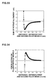
- a graph in which the distance r between the first and the second filler model Fm1, Fm2 is shown on the horizontal axis, and the sum of the potential energy is shown on the vertical axis is shown as the result of the calculation step.
- Fig. 34 a graph in which the distance r between the first and the second filler model Fm1, Fm2 is shown on the horizontal axis, and the force acting between the filler models is shown on the vertical axis is shown.
- the graph of Fig. 34 can be obtained by differentiating the curve of Fig. 33.
- the force acting between the first and the second filler models Fm1, Fm2 is substantially zero when the distance r between the first and the second filler models Fm1, Fm2 is approximately 0.39 nm.
- the present embodiment is useful in clearly understanding the interaction of the relevant fillers of the rubber composition filled with, for example, filler.
- the distance (dispersibility) between the fillers can be adjusted. Therefore, based on the calculation result of the interaction between the fillers, the dispersibility of the filler and the rubber is adjusted, and is useful in providing energetically stable filler filled rubber. Further, since the filler particle takes filler atom into consideration, a more suitable calculation result can be derived.
Applications Claiming Priority (8)
| Application Number | Priority Date | Filing Date | Title |
|---|---|---|---|
| JP2003358168 | 2003-10-17 | ||
| JP2003358168A JP3668239B2 (ja) | 2003-10-17 | 2003-10-17 | 粘弾性材料のシミュレーション方法 |
| JP2003358167A JP3668238B2 (ja) | 2003-10-17 | 2003-10-17 | ゴム材料のシミュレーション方法 |
| JP2003358167 | 2003-10-17 | ||
| JP2003386992 | 2003-11-17 | ||
| JP2003386992A JP3660932B2 (ja) | 2003-11-17 | 2003-11-17 | ゴム材料のシミュレーション方法 |
| JP2004014699 | 2004-01-22 | ||
| JP2004014699A JP4053994B2 (ja) | 2004-01-22 | 2004-01-22 | フィラー間相互作用のシミュレーション方法 |
Publications (3)
| Publication Number | Publication Date |
|---|---|
| EP1526468A2 true EP1526468A2 (fr) | 2005-04-27 |
| EP1526468A3 EP1526468A3 (fr) | 2006-07-19 |
| EP1526468B1 EP1526468B1 (fr) | 2009-09-30 |
Family
ID=34397123
Family Applications (1)
| Application Number | Title | Priority Date | Filing Date |
|---|---|---|---|
| EP04017402A Expired - Fee Related EP1526468B1 (fr) | 2003-10-17 | 2004-07-22 | Procédé de simulation d'un matériau viscoélastique |
Country Status (6)
| Country | Link |
|---|---|
| US (1) | US7415398B2 (fr) |
| EP (1) | EP1526468B1 (fr) |
| KR (1) | KR101083654B1 (fr) |
| CN (1) | CN1609884B (fr) |
| DE (1) | DE602004023360D1 (fr) |
| TW (1) | TWI339263B (fr) |
Cited By (6)
| Publication number | Priority date | Publication date | Assignee | Title |
|---|---|---|---|---|
| EP2535828A1 (fr) * | 2011-06-16 | 2012-12-19 | Sumitomo Rubber Industries, Ltd. | Procédé de simulation de la tangente de l'angle des pertes d'un composé de caoutchouc |
| EP2568284A3 (fr) * | 2011-09-09 | 2013-03-20 | Sumitomo Rubber Industries, Ltd. | Procédé permettant de simuler la déformation d'un composé de caoutchouc avec des particules de charge |
| EP2570808A3 (fr) * | 2011-09-14 | 2013-03-27 | Sumitomo Rubber Industries, Ltd. | Procédé permettant de simuler la déformation d'un composé de caoutchouc |
| EP2395339A4 (fr) * | 2009-02-03 | 2015-10-21 | Bridgestone Corp | Dispositif et méthode de prédiction du comportement des déformations de matériaux de caoutchouc |
| EP2778664A4 (fr) * | 2011-11-18 | 2015-12-23 | Sumitomo Rubber Ind | Procédé de simulation d'un matériau en caoutchouc |
| EP2500868A3 (fr) * | 2011-03-18 | 2017-08-30 | Sumitomo Rubber Industries, Ltd. | Procédé de création de modèle d'élément fini de composite en caoutchouc |
Families Citing this family (32)
| Publication number | Priority date | Publication date | Assignee | Title |
|---|---|---|---|---|
| US7130748B2 (en) * | 2001-07-18 | 2006-10-31 | Sri Sports Limited | Simulation method for estimating performance of product made of viscoelastic material |
| US7480205B2 (en) * | 2005-04-20 | 2009-01-20 | Landmark Graphics Corporation | 3D fast fault restoration |
| JP4833870B2 (ja) * | 2007-01-16 | 2011-12-07 | 富士通株式会社 | 非線形性の強い弾性体材料部材の解析モデル作成装置、解析モデル作成プログラム、解析モデル作成方法、および電子機器設計方法 |
| EP2481550B1 (fr) * | 2007-07-02 | 2014-10-08 | MAGMA Giessereitechnologie GmbH | Procédé de description de la distribution d'orientation statistique de particules dans une simulation de procédé de remplissage de moule et produit logiciel informatique pour la mise en oeuvre dudit procédé. |
| US8335669B2 (en) * | 2007-11-07 | 2012-12-18 | Bridgestone Sports Co., Ltd. | Golf ball and mechanical analysis of the same |
| BRPI1006973A2 (pt) * | 2009-01-30 | 2019-09-24 | Chevron Usa Inc | "sistema para prever fluxo de fluido em um reservatório subterrâneo, e, método implementado por computador." |
| US8296109B2 (en) * | 2009-04-20 | 2012-10-23 | Livermore Software Technology Corporation | Methods and systems for enabling simulation of aging effect of a chrono-rheological material in computer aided engineering analysis |
| JP4852626B2 (ja) * | 2009-04-28 | 2012-01-11 | 日東電工株式会社 | 応力−ひずみ曲線式を出力するためのプログラム及びその装置、並びに、弾性材料の物性評価方法 |
| JP5559594B2 (ja) | 2010-05-20 | 2014-07-23 | 住友ゴム工業株式会社 | ゴム材料のシミュレーション方法 |
| JP5039178B2 (ja) * | 2010-06-21 | 2012-10-03 | 住友ゴム工業株式会社 | 粘弾性材料からなる製品のシミュレーション方法 |
| US8825457B2 (en) | 2011-01-14 | 2014-09-02 | The Procter & Gamble Company | Systems and methods for material life prediction |
| US8972232B2 (en) | 2011-02-17 | 2015-03-03 | Chevron U.S.A. Inc. | System and method for modeling a subterranean reservoir |
| JP5752472B2 (ja) * | 2011-04-14 | 2015-07-22 | 東洋ゴム工業株式会社 | モデル作成装置、その方法及びそのプログラム |
| CN102306225B (zh) * | 2011-09-27 | 2013-01-09 | 上海大学 | 多线叠交隧道施工过程及对隧道变形影响数值模拟方法 |
| JP5503618B2 (ja) * | 2011-10-03 | 2014-05-28 | 住友ゴム工業株式会社 | ゴム材料のシミュレーション方法 |
| KR101293982B1 (ko) * | 2011-12-08 | 2013-08-07 | 현대자동차주식회사 | 탄성중합체의 시뮬레이션 방법 |
| JP5469696B2 (ja) * | 2012-03-19 | 2014-04-16 | 住友ゴム工業株式会社 | 高分子材料のエネルギーロスの計算方法 |
| US9135377B2 (en) * | 2012-04-16 | 2015-09-15 | Livermore Software Technology Corp. | Methods and systems for creating a computerized model containing polydisperse spherical particles packed in an arbitrarily-shaped volume |
| JP5466727B2 (ja) * | 2012-05-16 | 2014-04-09 | 住友ゴム工業株式会社 | 高分子材料のシミュレーション方法 |
| US9031822B2 (en) | 2012-06-15 | 2015-05-12 | Chevron U.S.A. Inc. | System and method for use in simulating a subterranean reservoir |
| EP3051444A4 (fr) * | 2013-10-07 | 2017-06-21 | Sumitomo Rubber Industries, Ltd. | Procédé de création de modèle d'élément fini pour un caoutchouc contenant une charge |
| JP5913260B2 (ja) * | 2013-11-14 | 2016-04-27 | 住友ゴム工業株式会社 | 高分子材料のシミュレーション方法 |
| JP6335101B2 (ja) * | 2014-04-18 | 2018-05-30 | 住友ゴム工業株式会社 | 高分子材料のシミュレーション方法 |
| US9805150B2 (en) * | 2014-07-30 | 2017-10-31 | The Boeing Company | Methods and systems for determining a structural parameter for noise and vibration control |
| KR20160024552A (ko) * | 2014-08-26 | 2016-03-07 | 삼성전자주식회사 | 입자로 구성된 변형체를 모델링하는 방법 및 장치 |
| CN106802969B (zh) * | 2015-11-26 | 2020-08-07 | 英业达科技有限公司 | 阻尼材料动态特性的验证系统及其验证方法 |
| JP6680564B2 (ja) * | 2016-02-29 | 2020-04-15 | 株式会社Ihi | 素材形状シミュレーション装置、素材形状シミュレーション方法及び三次元織繊維部品製造方法 |
| JP6891548B2 (ja) * | 2017-03-08 | 2021-06-18 | 横浜ゴム株式会社 | 複合材料の解析用モデルの作成方法、複合材料の解析用モデルの作成用コンピュータプログラム、複合材料の解析方法及び複合材料の解析用コンピュータプログラム |
| CN109856013B (zh) * | 2017-11-30 | 2021-09-14 | 廊坊立邦涂料有限公司 | 一种平整表面的半固体装饰性材料施工性能判断方法 |
| JP7290037B2 (ja) * | 2019-02-19 | 2023-06-13 | 住友ゴム工業株式会社 | ゴム材料のシミュレーション方法及びゴム材料の製造方法 |
| KR102605635B1 (ko) * | 2021-08-18 | 2023-11-24 | 한국과학기술원 | 나노 어스페리티의 순차적인 접촉 분석을 이용한 점착력 예측 방법 및 이를 수행하기 위한 프로그램을 기록한 기록 매체 |
| CN114722447B (zh) * | 2022-06-09 | 2022-11-01 | 广东时谛智能科技有限公司 | 多指触控展示鞋子模型方法、装置、设备及存储介质 |
Family Cites Families (23)
| Publication number | Priority date | Publication date | Assignee | Title |
|---|---|---|---|---|
| JP2775538B2 (ja) * | 1991-11-14 | 1998-07-16 | 住友重機械工業株式会社 | 成形シミュレーション方法及び装置 |
| EP0919941B1 (fr) * | 1997-11-25 | 2005-09-21 | Sumitomo Rubber Industries Limited | Méthode et appareil pour simuler un bandage pneumatique roulant |
| EP1030170B1 (fr) * | 1998-09-07 | 2005-03-30 | Bridgestone Corporation | Prediction de la performance d'un pneu |
| US6519536B1 (en) * | 1999-03-29 | 2003-02-11 | Pirelli Pneumatici S.P.A. | Method for determining the behaviour of a viscoelastic material |
| US6732057B2 (en) * | 2001-05-15 | 2004-05-04 | International Paper Company | Methods for engineering and manufacturing score-line-crack-resistant linerboard |
| JP3466585B2 (ja) | 2001-06-06 | 2003-11-10 | 住友ゴム工業株式会社 | 粘弾性材料からなる製品の性能予測のためのシミュレーション方法 |
| US6829563B2 (en) * | 2001-05-31 | 2004-12-07 | Sumitomo Rubber Industries, Ltd. | Simulation method for estimating performance of product made of viscoelastic material |
| JP3466584B2 (ja) | 2001-06-06 | 2003-11-10 | 住友ゴム工業株式会社 | 粘弾性材料からなる製品の性能予測のためのシミュレーション方法 |
| US7130748B2 (en) * | 2001-07-18 | 2006-10-31 | Sri Sports Limited | Simulation method for estimating performance of product made of viscoelastic material |
| WO2003011184A2 (fr) * | 2001-07-27 | 2003-02-13 | Medtronic,Inc. | Prothese vasculaire poreuse renforcee par un tissu adventice |
| US7311967B2 (en) * | 2001-10-18 | 2007-12-25 | Intel Corporation | Thermal interface material and electronic assembly having such a thermal interface material |
| US7147367B2 (en) * | 2002-06-11 | 2006-12-12 | Saint-Gobain Performance Plastics Corporation | Thermal interface material with low melting alloy |
| US20040107081A1 (en) * | 2002-07-12 | 2004-06-03 | Akio Miyori | Method of simulating tire and snow |
| JP3958666B2 (ja) * | 2002-10-11 | 2007-08-15 | Sriスポーツ株式会社 | 粘弾性材料に生じるエネルギーロスの算出方法、及び該方法を用いたゴルフボールのエネルギーロス評価方法 |
| US20040230411A1 (en) * | 2003-03-03 | 2004-11-18 | Moldflow Ireland Ltd. | Apparatus and methods for predicting properties of processed material |
| US7229683B2 (en) * | 2003-05-30 | 2007-06-12 | 3M Innovative Properties Company | Thermal interface materials and method of making thermal interface materials |
| JP3660932B2 (ja) | 2003-11-17 | 2005-06-15 | 住友ゴム工業株式会社 | ゴム材料のシミュレーション方法 |
| JP3668238B2 (ja) | 2003-10-17 | 2005-07-06 | 住友ゴム工業株式会社 | ゴム材料のシミュレーション方法 |
| JP3668239B2 (ja) | 2003-10-17 | 2005-07-06 | 住友ゴム工業株式会社 | 粘弾性材料のシミュレーション方法 |
| US7203604B2 (en) * | 2004-02-27 | 2007-04-10 | Bridgestone Firestone North American Tire, Llc | Method of predicting mechanical behavior of polymers |
| US7373284B2 (en) * | 2004-05-11 | 2008-05-13 | Kimberly-Clark Worldwide, Inc. | Method of evaluating the performance of a product using a virtual environment |
| JP4594043B2 (ja) * | 2004-11-15 | 2010-12-08 | 住友ゴム工業株式会社 | ゴム材料のシミュレーション方法 |
| JP4608306B2 (ja) * | 2004-12-21 | 2011-01-12 | 住友ゴム工業株式会社 | タイヤのシミュレーション方法 |
-
2004
- 2004-07-22 DE DE602004023360T patent/DE602004023360D1/de active Active
- 2004-07-22 EP EP04017402A patent/EP1526468B1/fr not_active Expired - Fee Related
- 2004-07-23 US US10/896,862 patent/US7415398B2/en active Active
- 2004-07-27 TW TW093122349A patent/TWI339263B/zh not_active IP Right Cessation
- 2004-09-02 CN CN2004100769195A patent/CN1609884B/zh not_active Expired - Fee Related
- 2004-09-06 KR KR1020040070751A patent/KR101083654B1/ko active IP Right Grant
Non-Patent Citations (9)
| Title |
|---|
| ALEKSEY D. DROZDOV, AL DORFMANN: "Finite viscoelasticity of filled rubbers: the effects of pre-loading and thermal recovery" CONTINUUM MECHANICS AND THERMODYNAMICS, vol. 14, no. 4, August 2002 (2002-08), pages 337-361, XP007900240 * |
| CATALDO FRANCO: "Model compound study about carbon black and diene rubber interaction: the reactivity of C60 fullerene with squalene" FULLERENE SCI TECHNOL; FULLERENE SCIENCE AND TECHNOLOGY 2000 MARCEL DEKKER INC, NEW YORK, NY, USA, vol. 8, no. 3, 2000, pages 153-164, XP009067086 * |
| CATALDO, F.: "The Role of Fullerene-like Structures in Carbon Black and Their Interaction with Dienic Rubber" FULLERENE SCIENCE AND TECHNOLOGY, vol. 8, no. 1/2, 2000, pages 105-112, XP009067093 * |
| DAVIS L C: "Model of magnetorheological elastomers" JOURNAL OF APPLIED PHYSICS, AMERICAN INSTITUTE OF PHYSICS. NEW YORK, US, vol. 85, no. 6, 15 March 1999 (1999-03-15), pages 3348-3351, XP012046944 ISSN: 0021-8979 * |
| GIRARD C ET AL: "van der Waals attraction between two C60 fullerene molecules and physical adsorption of C60 on graphite and other substrates" PHYSICAL REVIEW B (CONDENSED MATTER) USA, vol. 49, no. 16, 15 April 1994 (1994-04-15), pages 11425-11432, XP002382750 ISSN: 0163-1829 * |
| J.S. BERGSTRÖM, M.C. BOYCE: "Mechanical behavior of particle filled elastomers" RUBBER CHEMISTRY AND TECHNOLOGY, vol. 72, no. 4, 1999, pages 633-656, XP009063213 * |
| LU, W; TOMITA, Y: "Estimation of deformation behavior of rubber-blended glassy polymers" JOURNAL OF THE SOCIETY OF MATERIALS SCIENCE, JAPAN (JAPAN), vol. 50, no. 6, June 2001 (2001-06), pages 578-584, XP009063482 * |
| P. P. A. SMIT: "The glass transition in carbon black reinforced rubber" RHEOLOGICA ACTA, vol. 5, no. 5, December 1966 (1966-12), pages 277-283, XP009063221 * |
| VAN DOMMELEN J.A.W.1; BREKELMANS W.A.M.; BAAIJENS F.P.T.: "A numerical investigation of the potential of rubber and mineral particles for toughening of semicrystalline polymers" COMPUTATIONAL MATERIALS SCIENCE, vol. 27, no. 4, June 2003 (2003-06), pages 480-492, XP007900242 * |
Cited By (8)
| Publication number | Priority date | Publication date | Assignee | Title |
|---|---|---|---|---|
| EP2395339A4 (fr) * | 2009-02-03 | 2015-10-21 | Bridgestone Corp | Dispositif et méthode de prédiction du comportement des déformations de matériaux de caoutchouc |
| EP2500868A3 (fr) * | 2011-03-18 | 2017-08-30 | Sumitomo Rubber Industries, Ltd. | Procédé de création de modèle d'élément fini de composite en caoutchouc |
| EP2535828A1 (fr) * | 2011-06-16 | 2012-12-19 | Sumitomo Rubber Industries, Ltd. | Procédé de simulation de la tangente de l'angle des pertes d'un composé de caoutchouc |
| US9081921B2 (en) | 2011-06-16 | 2015-07-14 | Sumitomo Rubber Industries, Ltd. | Method for simulating rubber compound |
| EP2568284A3 (fr) * | 2011-09-09 | 2013-03-20 | Sumitomo Rubber Industries, Ltd. | Procédé permettant de simuler la déformation d'un composé de caoutchouc avec des particules de charge |
| EP2570808A3 (fr) * | 2011-09-14 | 2013-03-27 | Sumitomo Rubber Industries, Ltd. | Procédé permettant de simuler la déformation d'un composé de caoutchouc |
| US9097697B2 (en) | 2011-09-14 | 2015-08-04 | Sumitomo Rubber Industries, Ltd. | Method for simulating deformation of rubber compound |
| EP2778664A4 (fr) * | 2011-11-18 | 2015-12-23 | Sumitomo Rubber Ind | Procédé de simulation d'un matériau en caoutchouc |
Also Published As
| Publication number | Publication date |
|---|---|
| KR20050037342A (ko) | 2005-04-21 |
| US7415398B2 (en) | 2008-08-19 |
| CN1609884B (zh) | 2010-04-28 |
| EP1526468B1 (fr) | 2009-09-30 |
| EP1526468A3 (fr) | 2006-07-19 |
| DE602004023360D1 (de) | 2009-11-12 |
| CN1609884A (zh) | 2005-04-27 |
| TWI339263B (en) | 2011-03-21 |
| KR101083654B1 (ko) | 2011-11-16 |
| TW200515251A (en) | 2005-05-01 |
| US20050086034A1 (en) | 2005-04-21 |
Similar Documents
| Publication | Publication Date | Title |
|---|---|---|
| EP1526468B1 (fr) | Procédé de simulation d'un matériau viscoélastique | |
| KR101085174B1 (ko) | 고무 재료의 변형 시뮬레이션 방법 | |
| JP3668238B2 (ja) | ゴム材料のシミュレーション方法 | |
| Almeida et al. | Finite element formulations for hyperelastic transversely isotropic biphasic soft tissues | |
| Zhao et al. | Effects of particle asphericity on the macro-and micro-mechanical behaviors of granular assemblies | |
| Thornton et al. | Quasi-static shear deformation of a soft particle system | |
| JP6408856B2 (ja) | 高分子材料のシミュレーション方法 | |
| Beil et al. | Modeling and Computer Simulation of the Compressional Behavior of Fiber Assemblies: Part I: Comparison to Van Wyk's Theory | |
| JP6405183B2 (ja) | ゴム材料のシミュレーション方法 | |
| JP5432549B2 (ja) | ゴム材料のシミュレーション方法 | |
| JP3668239B2 (ja) | 粘弾性材料のシミュレーション方法 | |
| JP3660932B2 (ja) | ゴム材料のシミュレーション方法 | |
| Wu et al. | A twice-interpolation finite element method (TFEM) for crack propagation problems | |
| JP4697870B2 (ja) | 粘弾性材料のシミュレーション方法 | |
| JP6492438B2 (ja) | 特定物質の解析用モデルの作成方法、特定物質の解析用モデルの作成用コンピュータプログラム、特定物質のシミュレーション方法及び特定物質のシミュレーション用コンピュータプログラム | |
| Holtzman et al. | Mechanical properties of granular materials: A variational approach to grain‐scale simulations | |
| Luo et al. | Numerical estimation via remeshing and analytical modeling of nonlinear elastic composites comprising a large volume fraction of randomly distributed spherical particles or voids | |
| JP2009216612A (ja) | ゴム材料のシミュレーション方法 | |
| JP2005351770A (ja) | ゴム材料のシミュレーション方法 | |
| Goel et al. | A finite deformation nonlinear thermo-elastic model that mimics plasticity during monotonic loading | |
| JP7290037B2 (ja) | ゴム材料のシミュレーション方法及びゴム材料の製造方法 | |
| McGee et al. | Multiscale modelling of nanoindentation | |
| Zhong et al. | A new methodology for deformable object simulation | |
| Franken et al. | A tangential force-displacement model for elastic frictional contact between particles in triaxial test simulations | |
| JP2022139140A (ja) | フィラーモデルの作成方法 |
Legal Events
| Date | Code | Title | Description |
|---|---|---|---|
| PUAI | Public reference made under article 153(3) epc to a published international application that has entered the european phase |
Free format text: ORIGINAL CODE: 0009012 |
|
| AK | Designated contracting states |
Kind code of ref document: A2 Designated state(s): AT BE BG CH CY CZ DE DK EE ES FI FR GB GR HU IE IT LI LU MC NL PL PT RO SE SI SK TR |
|
| AX | Request for extension of the european patent |
Extension state: AL HR LT LV MK |
|
| PUAL | Search report despatched |
Free format text: ORIGINAL CODE: 0009013 |
|
| AK | Designated contracting states |
Kind code of ref document: A3 Designated state(s): AT BE BG CH CY CZ DE DK EE ES FI FR GB GR HU IE IT LI LU MC NL PL PT RO SE SI SK TR |
|
| AX | Request for extension of the european patent |
Extension state: AL HR LT LV MK |
|
| 17P | Request for examination filed |
Effective date: 20060814 |
|
| 17Q | First examination report despatched |
Effective date: 20070219 |
|
| AKX | Designation fees paid |
Designated state(s): DE FR GB |
|
| GRAP | Despatch of communication of intention to grant a patent |
Free format text: ORIGINAL CODE: EPIDOSNIGR1 |
|
| GRAS | Grant fee paid |
Free format text: ORIGINAL CODE: EPIDOSNIGR3 |
|
| GRAA | (expected) grant |
Free format text: ORIGINAL CODE: 0009210 |
|
| AK | Designated contracting states |
Kind code of ref document: B1 Designated state(s): DE FR GB |
|
| REG | Reference to a national code |
Ref country code: GB Ref legal event code: FG4D |
|
| REF | Corresponds to: |
Ref document number: 602004023360 Country of ref document: DE Date of ref document: 20091112 Kind code of ref document: P |
|
| PLBE | No opposition filed within time limit |
Free format text: ORIGINAL CODE: 0009261 |
|
| STAA | Information on the status of an ep patent application or granted ep patent |
Free format text: STATUS: NO OPPOSITION FILED WITHIN TIME LIMIT |
|
| 26N | No opposition filed |
Effective date: 20100701 |
|
| PGFP | Annual fee paid to national office [announced via postgrant information from national office to epo] |
Ref country code: GB Payment date: 20130717 Year of fee payment: 10 |
|
| GBPC | Gb: european patent ceased through non-payment of renewal fee |
Effective date: 20140722 |
|
| PG25 | Lapsed in a contracting state [announced via postgrant information from national office to epo] |
Ref country code: GB Free format text: LAPSE BECAUSE OF NON-PAYMENT OF DUE FEES Effective date: 20140722 |
|
| REG | Reference to a national code |
Ref country code: FR Ref legal event code: PLFP Year of fee payment: 13 |
|
| REG | Reference to a national code |
Ref country code: FR Ref legal event code: PLFP Year of fee payment: 14 |
|
| PGFP | Annual fee paid to national office [announced via postgrant information from national office to epo] |
Ref country code: FR Payment date: 20170613 Year of fee payment: 14 |
|
| PGFP | Annual fee paid to national office [announced via postgrant information from national office to epo] |
Ref country code: DE Payment date: 20170719 Year of fee payment: 14 |
|
| REG | Reference to a national code |
Ref country code: DE Ref legal event code: R119 Ref document number: 602004023360 Country of ref document: DE |
|
| PG25 | Lapsed in a contracting state [announced via postgrant information from national office to epo] |
Ref country code: FR Free format text: LAPSE BECAUSE OF NON-PAYMENT OF DUE FEES Effective date: 20180731 Ref country code: DE Free format text: LAPSE BECAUSE OF NON-PAYMENT OF DUE FEES Effective date: 20190201 |