WO2016133049A1 - 判定装置、判定方法および判定プログラム - Google Patents
判定装置、判定方法および判定プログラム Download PDFInfo
- Publication number
- WO2016133049A1 WO2016133049A1 PCT/JP2016/054311 JP2016054311W WO2016133049A1 WO 2016133049 A1 WO2016133049 A1 WO 2016133049A1 JP 2016054311 W JP2016054311 W JP 2016054311W WO 2016133049 A1 WO2016133049 A1 WO 2016133049A1
- Authority
- WO
- WIPO (PCT)
- Prior art keywords
- value
- reference model
- threshold
- determination
- time
- Prior art date
- Legal status (The legal status is an assumption and is not a legal conclusion. Google has not performed a legal analysis and makes no representation as to the accuracy of the status listed.)
- Ceased
Links
Images












Classifications
-
- G—PHYSICS
- G01—MEASURING; TESTING
- G01K—MEASURING TEMPERATURE; MEASURING QUANTITY OF HEAT; THERMALLY-SENSITIVE ELEMENTS NOT OTHERWISE PROVIDED FOR
- G01K11/00—Measuring temperature based upon physical or chemical changes not covered by groups G01K3/00, G01K5/00, G01K7/00 or G01K9/00
- G01K11/32—Measuring temperature based upon physical or chemical changes not covered by groups G01K3/00, G01K5/00, G01K7/00 or G01K9/00 using changes in transmittance, scattering or luminescence in optical fibres
-
- G—PHYSICS
- G01—MEASURING; TESTING
- G01K—MEASURING TEMPERATURE; MEASURING QUANTITY OF HEAT; THERMALLY-SENSITIVE ELEMENTS NOT OTHERWISE PROVIDED FOR
- G01K11/00—Measuring temperature based upon physical or chemical changes not covered by groups G01K3/00, G01K5/00, G01K7/00 or G01K9/00
- G01K11/32—Measuring temperature based upon physical or chemical changes not covered by groups G01K3/00, G01K5/00, G01K7/00 or G01K9/00 using changes in transmittance, scattering or luminescence in optical fibres
- G01K11/324—Measuring temperature based upon physical or chemical changes not covered by groups G01K3/00, G01K5/00, G01K7/00 or G01K9/00 using changes in transmittance, scattering or luminescence in optical fibres using Raman scattering
-
- G—PHYSICS
- G01—MEASURING; TESTING
- G01K—MEASURING TEMPERATURE; MEASURING QUANTITY OF HEAT; THERMALLY-SENSITIVE ELEMENTS NOT OTHERWISE PROVIDED FOR
- G01K3/00—Thermometers giving results other than momentary value of temperature
- G01K3/005—Circuits arrangements for indicating a predetermined temperature
-
- G—PHYSICS
- G01—MEASURING; TESTING
- G01M—TESTING STATIC OR DYNAMIC BALANCE OF MACHINES OR STRUCTURES; TESTING OF STRUCTURES OR APPARATUS, NOT OTHERWISE PROVIDED FOR
- G01M3/00—Investigating fluid-tightness of structures
- G01M3/002—Investigating fluid-tightness of structures by using thermal means
-
- G—PHYSICS
- G05—CONTROLLING; REGULATING
- G05B—CONTROL OR REGULATING SYSTEMS IN GENERAL; FUNCTIONAL ELEMENTS OF SUCH SYSTEMS; MONITORING OR TESTING ARRANGEMENTS FOR SUCH SYSTEMS OR ELEMENTS
- G05B23/00—Testing or monitoring of control systems or parts thereof
- G05B23/02—Electric testing or monitoring
- G05B23/0205—Electric testing or monitoring by means of a monitoring system capable of detecting and responding to faults
- G05B23/0218—Electric testing or monitoring by means of a monitoring system capable of detecting and responding to faults characterised by the fault detection method dealing with either existing or incipient faults
- G05B23/0243—Electric testing or monitoring by means of a monitoring system capable of detecting and responding to faults characterised by the fault detection method dealing with either existing or incipient faults model based detection method, e.g. first-principles knowledge model
-
- G—PHYSICS
- G05—CONTROLLING; REGULATING
- G05B—CONTROL OR REGULATING SYSTEMS IN GENERAL; FUNCTIONAL ELEMENTS OF SUCH SYSTEMS; MONITORING OR TESTING ARRANGEMENTS FOR SUCH SYSTEMS OR ELEMENTS
- G05B19/00—Program-control systems
- G05B19/02—Program-control systems electric
- G05B19/04—Program control other than numerical control, i.e. in sequence controllers or logic controllers
- G05B19/042—Program control other than numerical control, i.e. in sequence controllers or logic controllers using digital processors
- G05B19/0423—Input/output
- G05B19/0425—Safety, monitoring
-
- G—PHYSICS
- G05—CONTROLLING; REGULATING
- G05B—CONTROL OR REGULATING SYSTEMS IN GENERAL; FUNCTIONAL ELEMENTS OF SUCH SYSTEMS; MONITORING OR TESTING ARRANGEMENTS FOR SUCH SYSTEMS OR ELEMENTS
- G05B23/00—Testing or monitoring of control systems or parts thereof
- G05B23/02—Electric testing or monitoring
- G05B23/0205—Electric testing or monitoring by means of a monitoring system capable of detecting and responding to faults
- G05B23/0218—Electric testing or monitoring by means of a monitoring system capable of detecting and responding to faults characterised by the fault detection method dealing with either existing or incipient faults
- G05B23/0224—Process history based detection method, e.g. whereby history implies the availability of large amounts of data
- G05B23/0227—Qualitative history assessment, whereby the type of data acted upon, e.g. waveforms, images or patterns, is not relevant, e.g. rule based assessment; if-then decisions
- G05B23/0235—Qualitative history assessment, whereby the type of data acted upon, e.g. waveforms, images or patterns, is not relevant, e.g. rule based assessment; if-then decisions based on a comparison with predetermined threshold or range, e.g. "classical methods", carried out during normal operation; threshold adaptation or choice; when or how to compare with the threshold
Definitions
- This case relates to a determination device, a determination method, and a determination program.
- This case has been made in view of the above problems, and an object thereof is to provide a determination device, a determination method, and a determination program capable of determining a sign of abnormality.
- the determination apparatus includes a model creation unit that creates a reference model of the sensor detection value, and a predetermined time from a predetermined point in time until a deviation degree between the reference model and the sensor detection value exceeds a threshold value.
- a determination unit that determines whether or not the time is shorter than the time, and an output unit that outputs a signal related to abnormality when it is determined that the time is shorter.
- (A) And (b) is an example of the temperature measurement system by an optical fiber. It is a figure which illustrates an example of an objective variable and an explanatory variable group.
- (A) is the image figure which illustrated the difference of the estimated value at the time of using the fuel type A as a temperature difference
- (b) is the difference of the estimated value at the time of using the fuel type B, and an actual value. It is the image figure which illustrated as temperature difference. It is a figure which illustrates the relationship between a threshold value and abnormality determination.
- (A) is the schematic of the determination apparatus which concerns on 1st Embodiment
- (b) is a block diagram for demonstrating the hardware constitutions of a determination part. The explanatory variable group is illustrated.
- A is the schematic of the determination apparatus which concerns on 2nd Embodiment
- (b) is an example of a temperature sensor. It is an example of the flowchart performed when performing abnormality determination.
- A) is the actual value of the objective variable, and (b) is the actual value of the explanatory variable.
- (A) is an instantaneous value of the estimation error, (b) is an integrated value of the estimation error, and (c) is an estimated effective time. It is an example of a temperature sensor.
- (A) is the Mahalanobis distance, and (b) is the estimated effective time. It is a figure which illustrates the determination system of the modification 2.
- (A) And (b) is a figure which illustrates a sensor part and a measuring device.
- (A)-(c) is a figure which illustrates a sensor part. It is a figure which illustrates the flowchart showing a dimensionless procedure.
- (A) And (b) is a figure which illustrates an abnormality sign. It is an example of the flowchart performed when performing abnormality determination. It is a flowchart which illustrates a comparative example. It is a figure which illustrates the result of a comparative example.
- FIG. 21 is a diagram illustrating a result of the method described in FIG. 20.
- FIG. 21 is a diagram illustrating a result of the method described in FIG. 20. It is an example of the flowchart performed when performing abnormality determination. It is a figure which illustrates the result of abnormality determination. It is a figure which illustrates the normalized value of sensing data.
- abnormality can be determined at an early stage.
- a temperature sensor is arranged for a piping system in which a branch pipe is welded to the main pipe and gas or liquid leakage is detected early as a temperature change.
- an early temperature abnormality can be detected before a fire occurs even if a cooling failure occurs.
- Detecting a temperature abnormality includes, for example, a temperature measurement method using an optical fiber that measures Raman scattered light to obtain temperature information.
- leaking can be detected early as a temperature change by laying an optical fiber on a branch pipe.
- the cooling water temperature can be monitored by laying an optical fiber in the cooling water piping of the boiler. Thereby, even if a cooling failure occurs, an early temperature abnormality can be detected before a fire occurs.
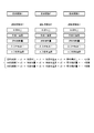
- FIG. 2 is a diagram illustrating an example of the objective variable and explanatory variable group.
- the objective variables 1 to 3 are the temperatures at various locations on the outer wall metal of the boiler.
- the explanatory variable group is an output value of the sensor having a correlation with the objective variable.
- the actual measurement values of the objective variables 1 to 3 can be obtained using a temperature sensor or the like installed on the outer wall metal.
- the estimation equations for the objective variables 1 to 3 are obtained by setting the coefficients and constants of each explanatory variable.
- coefficients and constants are based on the measured values of each past explanatory variable and objective variable, such as least square regression (Ordinary Least Mean Square), principal component regression (Principal Components Regression), partial least square regression (Partial Least Squares) etc.
- ⁇ Whether the system is normal or abnormal can be determined by comparing the measured value of the objective variable acquired at the same time with the estimated value of the estimation equation.
- the latest past data for a certain period is required. This latest period is referred to as a “modeling period”.
- the period during which the estimated value is actually compared with the actually measured value is referred to as a “scoring period”. If the “estimation error” exceeds a certain value during the scoring period, it is considered that a situation deviating from the estimation has occurred.
- FIG. 3A is an image diagram illustrating a difference in temperature between the estimated value and the actual value of the objective variable 1 and the objective variable 2 during the scoring period when the fuel type A is used.
- FIG. 3B is an image diagram illustrating, as a temperature difference, the difference between the estimated value and the actual value of the objective variable 1 and the objective variable 2 during the scoring period when the fuel type B is used.
- the threshold is 3 ⁇ and ⁇ 0.3 ° C.
- the threshold value is assumed to be ⁇ 0.9 ° C. at 3 ⁇ .
- 4 ⁇ is set, there is a possibility of overlooking an abnormality.
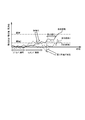
- FIG. 4 is a diagram illustrating the relationship between the threshold value and the abnormality determination.
- the threshold value when the threshold value is set to a relatively large threshold value 1, a delay occurs with respect to the case where a problem actually occurs, and the countermeasure is delayed. If the threshold value is set to a threshold value 2 that is smaller than the threshold value 1, it is determined to be abnormal in a situation different from the situation in which a problem actually occurs, so that the sign detection function cannot be performed. In other words, it is difficult to detect useful signs unless it is possible to “estimate sufficiently accurately, set a useful threshold value for each objective variable, and perform abnormality determination based on the threshold value”. It is not practical for business continuity to consider an appropriate threshold for each update of content that affects the threshold, such as periodic inspections and changes in the ratio of oil types.
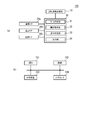
- FIG. 5A is a block diagram of the determination apparatus 100 according to the first embodiment.
- the determination device 100 is installed in a thermal power generation facility that uses a coal combustion cycle as an example.
- the determination apparatus 100 includes an explanatory variable acquisition unit 10, a plurality of temperature sensors 20a to 20c, a determination unit 30, and the like.
- the determination unit 30 includes a model creation unit 31, a threshold setting unit 32, an abnormality determination unit 33, and an output unit 34.
- FIG. 5B is a block diagram for explaining the hardware configuration of the determination unit 30.
- the determination unit 30 includes a CPU 101, a RAM 102, a storage device 103, an interface 104, and the like. Each of these devices is connected by a bus or the like.
- a CPU (Central Processing Unit) 101 is a central processing unit.
- the CPU 101 includes one or more cores.
- a RAM (Random Access Memory) 102 is a volatile memory that temporarily stores programs executed by the CPU 101, data processed by the CPU 101, and the like.
- the storage device 103 is a nonvolatile storage device.
- the storage device 103 for example, a ROM (Read Only Memory), a solid state drive (SSD) such as a flash memory, a hard disk driven by a hard disk drive, or the like can be used.
- the model creation unit 31, the threshold setting unit 32, the abnormality determination unit 33, and the output unit 34 are realized in the determination unit 30.
- the model creation unit 31, the threshold setting unit 32, the abnormality determination unit 33, and the output unit 34 may be hardware such as a dedicated circuit.
- the explanatory variable acquisition unit 10 acquires each explanatory variable.
- FIG. 6 illustrates the explanatory variable group.
- the explanatory variables are the electric energy, the coal supply amount, the internal temperature 1, the internal temperature 2, the air flow rate, the pressure 1, the pressure 2, the pressure 3, the ventilation port 1, the ventilation port 2, and the operation rotational speed. , Operating rate, operating frequency, etc.
- Each explanatory variable has a correlation with objective variables 1 to 3 (temperatures detected by the temperature sensors 20a to 20c). Moreover, it is preferable that each explanatory variable can be regarded as being independent from each other (low multicollinearity).
- the amount of electric power is generated electric power obtained by thermal power generation.
- the amount of coal supplied is the amount of coal supplied to the furnace.
- the internal temperatures 1 and 2 are, for example, temperatures at any location inside the furnace.
- the air flow rate is a flow rate of air supplied to the furnace.
- the pressures 1 to 3 are, for example, pressures in piping connected to the furnace.
- the ventilation openings 1 and 2 are the temperature of the ventilation openings.
- the operating speed, operating rate, and operating frequency are the operating speed, operating rate, and operating frequency of the furnace.
- the plurality of temperature sensors 20a to 20c are installed at different locations on the outside wall surface of the furnace, for example.
- temperature sensors are installed at three locations.
- a temperature measurement method of the temperature sensors 20a to 20c for example, a method using Raman scattered light in the optical fiber can be used.
- an optical fiber having a length of about 2 m is wound in a small area that can be regarded as almost the same temperature. By doing in this way, each winding part functions as one temperature sensor, respectively.
- the wall surface temperatures 1 to 3 detected by the temperature sensors 20a to 20c are used as measured values of the objective variables 1 to 3.
- the model creation unit 31 creates estimation equations for the objective variables 1 to 3 using the explanatory variables acquired by the explanatory variable acquisition unit 10 and the detection values of the temperature sensors 20a to 20c.
- This estimation formula is a reference model for objective variables 1 to 3.
- the estimation formula is obtained by setting the coefficients and constants of each explanatory variable, similarly to the estimation formula illustrated in FIG. These coefficients and constants can be set by regression analysis such as least square regression, principal component regression, and partial least square regression based on past explanatory variables and actual measurement values of the temperature sensors 20a to 20c. .
- the threshold value setting unit 32 sets a threshold value for the degree of deviation of the measured value of the objective variable from the reference model and the estimated effective time.
- an estimation error and an integrated value of the estimation error are used as the degree of divergence.
- the estimated value of the objective variable is a numerical value obtained by inputting an explanatory variable in the estimation formula.
- the estimation error related to the objective variable 1 is (actual value of the temperature sensor 20a) ⁇ (estimated value of the objective variable 1).
- the estimation error related to the objective variable 2 is (actual value of the temperature sensor 20b) ⁇ (estimated value of the objective variable 2).
- the estimation error related to the objective variable 3 is (actual value of the temperature sensor 20c) ⁇ (estimated value of the objective variable 3).
- the estimated effective time is a time from when the measurement of the estimation error is started in the scoring period using the reference model until one of the above divergence degrees exceeds the threshold.
- the abnormality determination unit 33 performs abnormality determination by determining whether or not the estimated effective time is below a threshold value.
- the output unit 34 outputs a signal related to abnormality when the abnormality determination unit 33 determines abnormality.
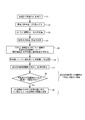
- FIG. 7 is a flowchart exemplifying processing for setting an objective variable estimation formula and setting a threshold value for the degree of deviation and the estimated effective time.
- the threshold value setting unit 32 first detects an initial condition update flag (step S1).
- the initial condition update flag is a flag that triggers an update of the objective variable estimation formula and the threshold values of the divergence degree and the estimated effective time.
- the threshold setting unit 32 sets appropriate allowable values 1 and 2 (step S2).
- the allowable value 1 is a threshold for the estimation error.
- the allowable value 2 is a threshold for the estimated error integrated value.
- the model creation unit 31 collects a data set for the modeling period (step S3).
- This data set includes explanatory variables and detection values (actual measurement values) of the temperature sensors 20a to 20c for each predetermined time in the modeling period.
- the model creation unit 31 determines the coefficients and constants of the estimation equations for the objective variables 1 to 3 using the data set collected in step S3 (step S4). By executing step S4, estimation equations for the objective variables 1 to 3 are set.
- the threshold setting unit 32 starts measurement of the estimation error (scoring period), for example, the first 60 times of the scoring period and the modeling period (30 minutes in the case of measurement of a 30-second period) estimation error An average value and a standard deviation are obtained (step S5).
- the threshold setting unit 32 resets the average value + 1 ⁇ value to 3 ⁇ value as the allowable value 1.
- the threshold setting unit 32 resets the allowable value 2 so that the estimated effective time is approximately 60 to 240 times the measurement cycle (30 minutes to 2 hours in the measurement at 30-second intervals) (step S6).
- step S6 if the scoring period is re-estimated before 30 minutes in the measurement at intervals of 30 seconds, it means that the allowable values 1 and 2 are small, and therefore it corresponds to relaxation.
- the threshold setting unit 32 sets a temporary threshold for the estimated effective time after the resetting in step S6, and starts a temporary measurement of the estimated error (step S7).
- the model creation unit 31 repeats re-creating the reference model when the estimation error exceeds the allowable value 1 or the integrated value of the estimation errors exceeds the allowable value 2.
- the threshold value setting unit 32 determines whether or not data to the extent that the re-creation is performed 30 times has been accumulated (step S8). If it is determined “No” in step S8, step S8 is executed again. If it is determined as “Yes” in step S8, the threshold setting unit 32 obtains the average value and standard deviation of the estimated effective time obtained in step S8, and resets the estimated effective time threshold using, for example, the 3 ⁇ value. (Step S9). In steps S6 to S9, the output unit 34 outputs a signal related to an abnormality if it falls below the threshold even during the provisional effective time.
- the threshold values for the allowable values 1 and 2 and the estimated effective time can be set as many times as you like by going back to the past with a pre-installed program once data is accumulated. Therefore, it is not necessary to perform data accumulation by performing data accumulation again when the allowable values 1 and 2 are reset, and to perform data accumulation by performing data accumulation again after resetting the estimated effective time threshold. Therefore, it is possible to construct a system in which only information that “changes have been made” is input to the system after periodic inspections, oil ratio change, and the like.
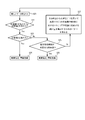
- FIG. 8 is an example of a flowchart executed when the abnormality determination unit 33 performs abnormality determination after the threshold values setting unit 32 sets the allowable values 1 and 2 and the estimated effective time threshold.
- the abnormality determination unit 33 collects the data set after the threshold values setting unit 32 sets the allowable values 1 and 2 and the estimated effective time threshold (step S11).
- the abnormality determination unit 33 determines whether or not the estimation error exceeds the allowable value 1 or the integrated value of the estimation error exceeds the allowable value 2 (step S12). If it is determined in step S12 that none of them is exceeded, step S12 is executed again.
- the abnormality determination unit 33 determines whether or not the estimated effective time is shorter than a predetermined time (for example, 10 minutes measured at 30 second intervals) (step S13). .
- a predetermined time for example, 10 minutes measured at 30 second intervals
- the output unit 34 outputs a signal related to the abnormality (Step S14).
- the abnormality determination unit 33 performs estimation again using past data from that time (for example, 1 hour by measurement at intervals of 30 seconds), and calculates coefficients and constants of the estimation formula. Update (step S15). Thereafter, the process is executed again from step S11.
- the allowable value 1 is an estimation error threshold
- the allowable value 2 is an integrated value for each update of the estimation error data. If a constant estimation is made, the average value of the estimation error will be almost zero if averaged over a long period of time. However, when a situation different from the estimation occurs, either the positive or negative value starts to increase.
- the threshold value set for this change is the allowable value 2. Even if the average value of estimation errors is close to zero, an event that suddenly starts to occur can be regarded as abnormal because the estimation error increases. The value in this case is the allowable value 1.
- the model creation unit 31 performs estimation again at that time, updates the coefficients and constants of the estimation formula, and restarts counting using the time as the estimation start time.
- the period until the next time the allowable value 1 or the allowable value 2 is exceeded is set as the “estimated effective time”, and a threshold is set for the “estimated effective time”.
- two allowable values are set, but one may be set or a larger number of settings may be performed. For example, after one or more tolerance values have been exceeded and one or more other tolerance values have been exceeded, the “estimated effective time” is determined and estimation is performed again. I do not care.
- the estimation error tends to be small after the creation of the reference model. If the estimation error is large in that state, it means that an event that is not considered in the formula has occurred. Therefore, if the “estimated effective time” is shortened, it can be determined that an abnormal situation has occurred even if the setting of the threshold and the ambiguity of the estimation are taken into consideration. That is, according to the present embodiment, a sign of abnormality can be determined.
- the threshold value of the deviation degree of the temperature sensors 20a to 20c with respect to the reference model is determined based on the deviation degree for a certain period after the creation of the reference model. In this case, the setting accuracy of the threshold value of the deviation degree is improved. Further, according to the present embodiment, the threshold value of the estimated effective time is determined based on time variation until the deviation degree exceeds the threshold value. In this case, the setting accuracy of the threshold for the estimated effective time is improved.
- the reference model is created using the sensor detection value and the detection values of a plurality of other sensors having a correlation with the sensor detection value.
- the present invention is not limited to this.
- a reference model of sensor detection values is created using correlations between detection values of a plurality of sensors.
- a sign detection method that finds signs of abnormality at an early stage from the correlation of temperature transition data detected by multiple temperature sensors.
- a method for obtaining the Mahalanobis square distance calculated from the mean and variance-covariance matrix of the target data group, an MSD method for robustly estimating the center and spread of the data, and obtaining a statistic corresponding to the Mahalanobis square distance, etc. Can be used.
- Tn (t) is shown in the following (1) to (3).
- a modeling period (a fixed period in which data is accumulated that is older than the current time) is set, and the average of the temperature data of each of the n temperature sensors in that period and the inverse covariance matrix of the temperature data group are reversed. Find the matrix.
- the procedure for setting a modeling period, determining a threshold value from the period, and sequentially comparing a new data set with the threshold value is the same. That is, even in the sign detection by “outlier detection” using the correlation between the measurement data, the accuracy of the sign detection is determined by setting the threshold value. In other words, it is difficult to detect useful signs unless it is possible to “estimate with sufficiently high accuracy, set a useful threshold value, and perform abnormality determination based on the threshold value”. Therefore, in the second embodiment, a determination device, a determination method, and a determination program that can determine a sign of abnormality will be described.
- FIG. 9A is a schematic diagram of the determination apparatus 100a according to the second embodiment.
- the difference between the determination apparatus 100a and the determination apparatus 100 of the first embodiment is that the explanatory variable acquisition unit 10 is not provided and the temperature sensor 20 is provided instead of the temperature sensors 20a to 20c.
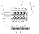
- the temperature sensor 20 detects temperatures at a plurality of locations where the temperature values are correlated with each other. For example, as illustrated in FIG. 9B, the temperature sensor 20 detects the temperature at each location based on the result obtained by backscattered light at different length positions of the same optical fiber. In the example of FIG. 9B, each winding unit functions as an individual temperature sensor.
- the configuration of the determination unit 30 is the same as that in the first embodiment.
- the model creation unit 31 creates a reference model by obtaining the Mahalanobis square distance calculated from the average of the detected values at each location detected by the temperature sensor 20 and the variance-covariance matrix.
- the model creation unit 31 creates a reference model by using a MSD method or the like that robustly estimates the center and spread of the detection value and obtains a statistic corresponding to the Mahalanobis square distance.
- the reference model here is the center of variation reflecting the magnitude of the correlation between a plurality of detected values (orientation when paying attention to each of the two sensors).
- the threshold value setting unit 32 sets a threshold value for the degree of deviation of the measured value of the sensor detection value from the reference model and the estimated effective time.
- the degree of divergence of the actual measurement value of the objective variable with respect to the reference model is the Mahalanobis square distance, the integrated value for each data update of the Mahalanobis square distance, or the like. In the present embodiment, the Mahalanobis square distance and the integrated value of the Mahalanobis square distance are used as the divergence.
- the estimated effective time is the time from the start of measurement of Mahalanobis square distance in the scoring period after creation of the reference model until any of the above divergences exceeds a threshold value.
- the abnormality determination unit 33 performs abnormality determination by determining whether or not the estimated effective time is below a threshold value.
- the output unit 34 outputs a signal related to abnormality when the abnormality determination unit 33 determines abnormality.
- the setting of the reference model and the setting of the divergence degree and the threshold of the estimated effective time can be performed by the same processing as in FIG.
- the threshold value setting unit 32 sets an allowable value 3 in addition to the allowable values 1 and 2 in advance.
- FIG. 10 is an example of a flowchart executed when the abnormality determination unit 33 performs abnormality determination after the threshold values setting unit 32 sets the allowable values 1 and 2 and the estimated effective time threshold.
- the abnormality determining unit 33 collects the data set after the threshold values setting unit 32 sets the allowable values 1 and 2 and the estimated effective time threshold (step S21). This data set is collected for each detection value at each location of the temperature sensor 20.
- the abnormality determination unit 33 determines whether the Mahalanobis square distance at any location exceeds the allowable value 1 or whether the integrated value of the Mahalanobis square distance at the location exceeds the allowable value 2 (step S22). ). If it is determined in step S22 that none of them is exceeded, step S22 is executed again. When it is determined in step S22 that any of the distances has exceeded, the abnormality determination unit 33 determines whether the Mahalanobis square distance has exceeded the allowable value 3 (step S23).
- step S24 If it is determined “Yes” in step S23, the output unit 34 outputs a signal related to the abnormality (step S24).
- the abnormality determination unit 33 determines whether or not the estimated effective time is less than a predetermined time (for example, 10 minutes in measurement at intervals of 30 seconds) (step S25). .
- a predetermined time for example, 10 minutes in measurement at intervals of 30 seconds
- the abnormality determination unit 33 again corresponds to the Mahalanobis square distance or the Mahalanobis square distance in the MSD method using the past data (for example, one hour at a measurement of 30 seconds).
- the parameter for deriving the statistics to be obtained is obtained (step S27). Parameters in this case include an average value, an unbiased covariance matrix, an inverse matrix, and the like in a new modeling period at each location of the temperature sensor 20. Thereafter, the process is executed again from step S21.
- the Mahalanobis square distance exceeds the tolerance value 1 or the integrated value exceeds the tolerance value 2, the new data group is used for estimation again.
- the allowable value 3 is exceeded, an abnormality is determined.
- the method of deriving the Mahalanobis square distance there is a method of comparing the Mahalanobis square distance obtained sequentially with the allowable value 1 and comparing the integrated value of the Mahalanobis square distance with the allowable value 2. For example, when the temperature is measured at a plurality of points and the temperature at the plurality of points is changed to a dangerous temperature, the Mahalanobis square distance is small, but it can be said to be an abnormal state.
- an allowable value 3 is set and compared with the measurement data itself.
- the allowable value 3 may not be a fixed value, but may be a unique value for each number of measurement points.
- the setting number and setting method of the allowable value are not limited to the example of FIG.
- the threshold value of the divergence degree of each detection value of the temperature sensor 20 with respect to the reference model is determined based on the divergence degree for a certain period after the creation of the reference model. In this case, the setting accuracy of the threshold value of the deviation degree is improved.
- the threshold of the estimated effective time is determined based on time variation until the divergence degree exceeds the threshold. In this case, the setting accuracy of the threshold for the estimated effective time is improved.
- Example 1 the same objective variables and explanatory variables as in FIG. 6 were used according to the first embodiment.
- the system according to the first embodiment is intended to predict whether the wall surface temperatures 1 to 3 are maintained in an appropriate range from the explanatory variable group and to rotate the operation cycle in the most efficient state. If the operation cycle becomes too high and high pressure, combustion before the boiler occurs, and if it becomes too low, the combustion efficiency in the boiler decreases. It is required to control the optimal temperature and pressure while avoiding combustion.
- the threshold values were set as follows according to the processing of FIG. In this embodiment, the same numerical values are used for the objective variables 1 to 3. Tolerance 1 ⁇ 2 ° C Tolerance 2 ⁇ 10 ° C Valid time threshold Less than 20 minutes
- a 14-by-14 variance-covariance matrix is generated using the explanatory variable group in the modeling period and the value of the objective variable 1. Specifically, it is arranged at the last stage so that the variance of the objective variable 1 is in the 14th row and the 14th column.
- (2) Generate an inverse matrix for 13 rows and 13 columns excluding the row / column of the objective variable.
- (3) The product obtained by excluding the inverse matrix obtained in (2) and the 14th column element in the 14th column obtained in (1) is obtained to obtain 13 numerical values. To do.
- system failure is substituted by system operation stop.
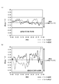
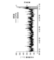
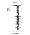
- system operation stop As illustrated in FIG. 11A and FIG. 11B, the operating state of the system is changed from around 17:20, but no particular abnormality has occurred, but each explanatory variable at 18:18. Fluctuates rapidly. This is because the operation of the system is stopped. If this 18:18 system operation stoppage can be estimated as soon as possible for several minutes, the system is effective.
- FIG. 12 (a) shows an instantaneous value of the estimation error.
- FIG. 12B shows an integrated value of estimation errors.
- FIG. 12C shows the estimated effective time. The position where the integrated value is reset to zero in FIG. 12B and the data position in FIG. 12C are the same. This is because at that time, the instantaneous value in FIG. 12A exceeds the allowable value 1 or the integrated value in FIG. 12B exceeds the allowable value 2 and the re-estimation calculation is performed.
- the estimation error immediately after the start of re-estimation is small.
- 11A, 11B, and 12C the estimated effective time gradually decreases toward 18:18, and the point of 18:12 is 16 minutes after 17:55.
- the automatic determination of this abnormality is reasonable. This means that the abnormality has been confirmed 6 minutes before 18:18, and the system can be promptly stopped.
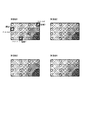
- Example 2 is an example according to the second embodiment. As illustrated in FIG. 13, four sets of wound portions were created and brought into close contact with the furnace wall. Each of these four sets was used as a temperature sensor. In FIG. 13, a portion drawn with a circle is a wound portion, and each wound portion is connected by the same optical fiber. In addition, the temperature distribution is drawn using a mesh pattern. The coarse mesh portion has a low temperature, and the fine mesh portion has a high temperature. If excessive heat accumulation partially starts inside each device, the temperature rises partially, so that an abnormality can be detected.
- Winding part set 1 region 1 (X1a1, Z1a1), (X1a2, Z1a2) Region 2 (X1b1, Z1b1), (X1b2, Z1b2) Region 3 (X1c1, Z1c1), (X1c2, Z1c2) Winding part set 2 region 1 (X2a1, Z2a1), (X2b2, Z2a2) Region 2 (X2b1, Z2b1), (X2b2, Z2b2)
- the area is specified as follows.
- the average value, the maximum value, the minimum value, etc. are obtained from the temperature at each position of the optical fiber included in each region, and this is used as temperature data for each region.
- a threshold value is provided for each of these 12 temperatures, and this is set to an allowable value of 3. In this example, since the temperature corresponding to the allowable value 3 was not exceeded, only the allowable values 1 and 2 and the effective time threshold were set.
- Allowable value 1 is set for the value of Mahalanobis square distance for the data in the modeling period used at the time of the new data set.
- the allowable value 2 is set with respect to the average value of the Mahalanobis square distance one sample before and the Mahalanobis square distance of the new data set.
- the Mahalanobis square distance indicates how far the new data set is from the center of gravity of the data set during the modeling period.
- the Mahalanobis square distance takes into account the vector component in any direction, and if it is added, the data set is updated so that it rotates with a constant distance around the center of gravity, and it moves to a different quadrant across the center of gravity.
- Such cases can be indicated by different numerical values. However, this is because they are considered to be the same in scalar addition.
- the average value is adopted as the allowable value 2 under the assumption that the neighboring data goes in the same direction if the data set gradually deviates. Allowable value 1 60 Allowable value 2 50 Valid time threshold Less than 20 minutes
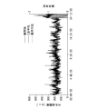
- FIG. 14A and FIG. 14B illustrate results of predictive detection by obtaining the Mahalanobis square distance.
- the Mahalanobis square distance is the shortest immediately after the modeling period.
- the Mahalanobis distance increases as time elapses, but the increasing tendency is different in each time zone.
- the estimated effective time of 50 minutes in the 17:04 re-estimation becomes shorter thereafter, the estimated effective time of the 17:54 re-estimation is 14 minutes, and the estimated effective time of the 18:08 re-estimation is 8 minutes. It is.
- the abnormality was confirmed at 18:08, 14 minutes after 17:54. This is a stage 10 minutes earlier than 18:18 when the system is shut down. In this example, the system shut down is described, but even if there is actually any sign of an accident, the time when the initial action can be taken. The possibility that can be secured was found.
- the temperature measuring method of the plurality of temperature sensors 20a to 20c or the temperature sensor 20 is a method using Raman scattered light in the optical fiber, but is not limited thereto. Absent.
- a thermocouple, a resistance temperature detector, a camera imaging type infrared thermography, or the like is used as the temperature sensors 20a to 20c or the temperature sensor 20.
- thermocouple for each measurement point, it is necessary to have two conductors in which insulation between the conductors and between each conductor and the wall surface is maintained.
- the surface to be measured is not kept warm, it is in a state where it can be imaged from the outside without any obstruction, and a plurality of temperature data in the vicinity of the position corresponding to the measurement point It is necessary to combine them into one measurement point by averaging, etc., and to obtain the emissivity of the outer wall surface in advance for accurate conversion from luminance to temperature.
- the temperature is the target variable and the other sensing data is the explanatory variable.
- the temperature to be measured is determined by determining the target variable from the other sensing data.
- An explanatory variable may be used together with the data. Since it is only what kind of value to focus on, for example, it may be a usage method in which the power generation system is used as the objective variable and if an abnormal sign is detected, the efficiency of the power generation system is degraded. .
- the above embodiment may be applied to other sensing data instead of the temperature sensor 20. This will be described in Example 4 described later.
- FIG. 15 is a diagram illustrating a determination system according to the second modification.
- the determination unit 30 acquires data directly from the temperature sensor 20.
- a server having a function of a determination unit acquires data from a temperature sensor through an electric communication line.
- the determination system of Modification 2 includes a temperature sensor 20, a server 202, and a monitoring server 203.
- the temperature sensor 20 includes a sensor unit 21 for acquiring temperature data of an object to be measured, and a measuring device 22 that acquires measurement data from the sensor unit 21 and generates temperature data.
- the temperature sensor 20 has a configuration connected to a server 202 through an electric communication line 201 such as the Internet.
- a monitoring server 203 that monitors the measurement object on which the sensor unit 21 is installed is connected to the telecommunication line 201.
- the server 202 includes the CPU 101, the RAM 102, the storage device 103, the interface 104, and the like illustrated in FIG. 5B, and realizes a function as the determination unit 30.
- the server 202 installed in Japan receives measurement data measured by a coal bunker of a power plant in another country, and detects a sign of abnormal heat generation in the coal bunker. A result output from the server 202 is transmitted to the monitoring server 203.
- This modification can also be applied to the first embodiment.
- a plurality of temperature sensors 20a to 20c may be used instead of the temperature sensor 20.
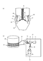
- FIG. 16A and FIG. 16B are diagrams illustrating the sensor unit 21 and the measuring device 22.
- the sensor unit 21 is attached to the outer wall of a mill intermediate housing unit 40 of a pulverized coal machine for pulverizing coal to produce fine powder, for example.
- the mill intermediate housing portion 40 includes a storage portion 42 in which the coal 41 falls and temporarily stored, and a pulverization ring that pulverizes the coal 41 stored in the storage portion 42. 43 and a roller 44.
- the pulverized coal 45 obtained by the pulverization is raised by the air in the primary air chamber 46.
- the measuring device 22 includes a laser 11, a beam splitter 12, an optical switch 13, a filter 14, a plurality of detectors 15a and 15b, a calculation unit 16, and the like.
- the laser 11 is a light source such as a semiconductor laser, and emits laser light in a predetermined wavelength range. For example, the laser 11 emits light pulses (laser pulses) at predetermined time intervals.
- the beam splitter 12 makes the optical pulse emitted from the laser 11 enter the optical switch 13.
- the optical switch 13 is a switch for switching an emission destination (channel) of an incident optical pulse. In the double-end method, the optical switch 13 makes light pulses alternately enter the first end and the second end of the optical fiber 23 of the sensor unit 21 at a constant period. In the single end system, the optical switch 13 makes an optical pulse incident on either the first end or the second end of the optical fiber 23.
- the optical fiber 23 is arranged along a predetermined path for temperature measurement.
- the light pulse incident on the optical fiber 23 propagates through the optical fiber 23.
- the light pulse gradually attenuates and propagates through the optical fiber 23 while generating forward scattered light traveling in the propagation direction and back scattered light (return light) traveling in the feedback direction.
- the backscattered light passes through the optical switch 13 and enters the beam splitter 12 again.
- the backscattered light incident on the beam splitter 12 is emitted to the filter 14.
- the filter 14 is a WDM coupler or the like, and extracts a long wavelength component (Stokes component) and a short wavelength component (anti-Stokes component) from the backscattered light.
- the detectors 15a and 15b are light receiving elements.
- the detector 15 a converts the received light intensity of the short wavelength component of the backscattered light into an electric signal and transmits it to the computing unit 16.
- the detector 15 b converts the received light intensity of the long wavelength component of the backscattered light into an electrical signal and transmits it to the computing unit 16.
- the computing unit 16 measures the temperature distribution in the drawing direction of the optical fiber 23 using the Stokes component and the anti-Stokes component.
- FIG. 17 (a) is a transparent view of the sensor unit 21, and is a view through the sheet 24b of FIG. 17 (b).
- FIG. 17B is a cross-sectional view taken along the line AA in FIG.
- the sensor unit 21 is a fiber sheet in which the optical fiber 23 is disposed at a predetermined position. As illustrated in FIGS. 17A and 17B, the sensor unit 21 includes a pair of sheets 24a and 24b that are held with the optical fiber 23 interposed therebetween, and a glass cloth tape that maintains a gap between the sheets 24a and 24b. 25 and a metal tube 27 with a slit that roughly determines the position of the winding portion 26 of the optical fiber 23.
- the optical fiber 23 has wound portions 26a to 26h (hereinafter collectively referred to as a wound portion 26) held by the sheets 24a and 24b in a state of being wound a plurality of times.
- FIG. 17C shows an example in which the optical fiber 23 is wound in a single layer.
- the winding portions 26a to 26h are constituted by one optical fiber 23, or are constituted by two optical fibers 23, one at each of the upper and lower stages. In the latter case, for example, the fusion connection is performed at the upper and lower connection portions in FIG.
- the sheet 24a is in contact with the measurement target.
- An adhesive tape 28 is provided on the sheet 24a. Thereby, the sheet 24a can be attached to the temperature measurement object.
- the winding portions 26a to 26h are wound, for example, 2 to 8 times, respectively.
- the diameter of the optical fiber 23 varies depending on the heat-resistant temperature, but is 0.16 to 0.4 mm. About 1 to 2 mm, which is more than twice the diameter, is required. Since the thickness of the metal tube 27 is about 0.5 mm, it has a thickness of about 2 to 3 mm from the sheet 24a to 24b.
- the average value, the maximum value, the minimum value, and the like are obtained from the temperature at each position of the optical fiber included in each region, and are used as temperature data for each region.
- the part 26 has a thickness as shown in FIG. 17B, and the temperature of the winding part 26 away from the measurement target may deviate greatly from the actual temperature of the measurement target.
- a predetermined number of points for example, five points in order from the highest temperature value are selected to obtain an average value, It is set as the temperature of the area
- the third embodiment will be described as an embodiment that holds an object different from that of the second embodiment.
- the second embodiment illustrated in FIG. 10 it is assumed that various sensing data is used, but a specific method thereof is not shown. Therefore, in the present embodiment, an example of the method is first shown.
- This method itself is the same as that disclosed in Japanese Patent No. 5308501 as conversion to a random variable, and is a general method in ordinary multivariate analysis.
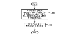
- FIG. 18 is a diagram illustrating a flowchart representing a dimensionless procedure when modeling is performed using N sensing data S1 (t) to SN (t) at time t.
- This dimensionless procedure is performed when the model creation unit 31 executes step S3 and step S4 in FIG. 7 and when the abnormality determination unit 33 executes step S15 in FIG. 8 or step S27 in FIG.
- N pieces of sensing data S1 (t) to SN (t) are each objective variable and each explanatory variable.
- the model creation unit 31 is the main component will be described.
- the model creation unit 31 obtains the average value and standard deviation of each sensing data in a predetermined past time (modeling period) from the current reference time t (step S31).
- the average values S1_ave to SN_ave of the N pieces of sensing data S1 (t) to SN (t) at time t from the time t0 to the predetermined past time ⁇ T used for modeling are expressed by the following equations.
- S1_ave Average (S1 (t0),..., S1 (t0 ⁇ T))
- S2_ave Average (S2 (t0),..., S2 (t0 ⁇ T)), ...
- the model creation unit 31 first subtracts each average value from each sensing data value to obtain a zero reference value, and further divides by a standard deviation value or a value that is a multiple of that value (step S32). ). Thereby, each sensing data is made dimensionless.
- the abnormality determination unit 33 performs the dimensionless procedure, the dimensionless process is performed on the new data group when executing step S11 in FIG. 8 or step S21 in FIG.
- the average value of each sensing data becomes zero during the modeling period, and the variation of the values becomes uniform. Variations in values can be corrected by later parameter derivation methods, so the standard deviation value is not used, and each sensing data value is divided by the calculated average value, and the parameter is derived using the resulting value. Good. In that case, the average value in the modeling period is 1.
- sensing data having different dimensions such as the wall temperature 1 to 3, the amount of electric power, the amount of coal supplied, the pressure 1 to 3 and the like illustrated in FIG. 6 can be handled by the methods of FIGS. It becomes possible.
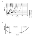
- FIG. 19A shows that abnormal signs in the plant do not converge immediately after a single event occurs, but are exemplified in the spontaneous combustion phenomenon of coal illustrated in FIG. 19A or in FIG. 19B.
- the bearing deteriorates gradually, it begins to occur frequently at an accelerated rate, and it becomes a continuous phenomenon leading to an accident. This is a sudden occurrence seen in actual power plants and plants. Therefore, it is necessary to separate it from the case where some kind of abnormality occurs for a short period of time and then it becomes normal immediately after that.
- FIG. 19 (a) shows that the spontaneous combustion phenomenon frequently occurs at an accelerated rate in any of the coal types A to H.
- the procedure of FIG. 20 is disclosed as one method of the present embodiment.
- the apparatus configuration is the same as that of the second embodiment.
- the abnormality determination unit 33 collects the data set after the threshold values setting unit 32 sets the allowable values 1 and 2 and the estimated effective time threshold (step S41). This data set is collected for each detection value at each location of the temperature sensor 20.
- the abnormality determination unit 33 determines whether or not the Mahalanobis square distance at any location exceeds the allowable value 1 and the integrated value of the Mahalanobis square distance at the location exceeds the allowable value 2 (step S42). . If “No” is determined in step S42, the process is executed again from step S41. When it is determined as “Yes” in step S42, the abnormality determination unit 33 determines whether or not the Mahalanobis square distance exceeds the allowable value 3 (step S43).
- step S43 the output unit 34 outputs a signal related to the abnormality (step S44). If it is determined as “No” in step S43, the abnormality determination unit 33 again corresponds to the Mahalanobis square distance or the Mahalanobis square distance in the MSD method using past data (for example, one hour at a measurement of 30 seconds). A parameter for deriving a statistic to be obtained is obtained (step S45). Parameters in this case include an average value, an unbiased covariance matrix, an inverse matrix, and the like in a new modeling period at each location of the temperature sensor 20.
- the abnormality determination unit 33 starts an outlier test in the following steps S47 and S48 using the current data set collected in step S41 (step S46).
- the abnormality determination unit 33 determines whether or not the Mahalanobis square distance at any location exceeds the allowable value 1 and the integrated value of the Mahalanobis square distance at the location exceeds the allowable value 2 (step S47).
- the abnormality determination unit 33 determines whether or not the estimated effective time is less than a predetermined time (for example, 10 minutes measured at 30 second intervals) (Step S48). . If it is determined as “Yes” in step S48, the abnormality determination unit 33 outputs a signal related to the abnormality (step S49).
- step S47 the abnormality determination unit 33 sets the estimated effective time to a fixed value that is larger than the predetermined time (step S50). Thereafter, the process is executed again from step S41.
- Step S48 the abnormality determination unit 33 resets the estimated effective time to zero (Step S51). Thereafter, the process is executed again from step S41.
- the outlier test is not performed using the new data set after modeling, but the outlier test is performed again on the current data set, and the estimated effective time is reset based on the result. Decide whether or not. This is because when a certain amount of time has passed without modeling, if the new data set exceeds tolerance 1 or tolerance 2, it is actually due to the occurrence of a sudden event. This is to determine whether it has been made or simply caused by a change in coal type or output command. This technical idea can also be applied to the first embodiment. If the allowable value 1 or allowable value 2 is exceeded again after modeling, it may be considered to be equivalent to the former. It will be possible to judge.
- step S42 and step S47 of FIG. 20 “and” determination may be “or” determination.
- the third embodiment illustrated in FIG. 20 is compared with the comparative example of FIG. 21 in which modeling is always performed before the outlier test, which is a standard moving window used in Japanese Patent No. 5308501.
- the effects of the third embodiment will be clarified.
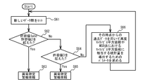
- using the set data group step S61
- when the Mahalanobis distance at any location exceeds the allowable value 1 and the allowable value 2 step S62
- a signal relating to abnormality is output.
- Step S63 If the Mahalanobis distance exceeds the allowable value 3 in the case of “No” in step S62 (step S64), a signal relating to the abnormality is output (step S65).
- step S 64 a statistic corresponding to the Mahalanobis square distance or the Mahalanobis square distance in the MSD method is derived again using the past data (for example, 1 hour at 30 second intervals) from that point.
- a parameter is obtained (step S66).
- the dimensionless processing illustrated in FIG. 18 was performed.
- the method of dividing by the average value is used instead of the method of dividing by the standard deviation, which is another method described above.
- the thermal power generation facility using the coal combustion cycle shown in the first embodiment as an object is taken as an example.
- the sheet processed as shown in FIGS. 9 (b), 13 and 17 having a large number of winding portions is installed on the wall surface of the facility as shown in FIG. 64 points of measurement data are extracted and treated as a data set for each measurement.
- FIG. 22 illustrates the result of the comparative example.
- the instantaneous value is an outlier distance calculated using a new data set
- the two-point average is a two-point average value of the previously calculated outlier distance and the currently calculated outlier distance.
- Allowable value 1 is the average value of the instantaneous value of the model update period + 3 times the standard deviation of the instantaneous value (3 ⁇ )
- allowable value 2 is the average value of the 2-point average value + 3 times the standard deviation of the instantaneous value (3 ⁇ ) Value.
- the allowable value 3 was an average value of instantaneous values + 8 times (8 ⁇ ) a standard deviation of instantaneous values.
- 0 is output when there is no abnormality in FIG.
- abnormality determination frequently occurs at 18:14, which is four minutes faster than 18:18 when the system is stopped.
- erroneous detection occurs three times from midnight, and it can be seen that the reliability of the system is impaired.
- FIG. 23 illustrates the result of the method described in FIG. Definitions of instantaneous value, two-point average, abnormality determination, and allowable values 1 to 3 are the same as those in FIG.
- the threshold for the estimated effective time was 4 minutes. Abnormality judgment frequently occurs at 18:16, which is 2 minutes earlier than 18:18 when the system is stopped, but 2 minutes later than the method of FIG. However, unlike FIG. 22, it can be seen that there is no false detection and the reliability of abnormality determination is maintained.
- the allowable value 1 is the average value of the instantaneous value + the standard deviation of the instantaneous value (2 ⁇ )
- the allowable value 2 is the average value of the two-point average + the standard deviation of the instantaneous value.
- FIG. 24 and FIG. 25 show what has been changed to a double (2 ⁇ ) value. In either case, the time at which the abnormality determination starts frequently does not change as in FIGS. In the method shown in FIG. 21, further erroneous detection occurs more frequently, but in the method shown in FIG. 20, it can be seen that no erroneous detection occurs and the reliability of abnormality determination is maintained.
- the allowable value 1 and 2 are the average value + twice the standard deviation (2 ⁇ ) to the standard. Even if it is set with an ambiguous width of 3 times the deviation (3 ⁇ ), it can be said that the sign detection can be performed.
- Example 4 not only the temperature but also detection of the abnormal sign illustrated in FIG. 26 is performed on various sensing data of the thermal power generation facility that uses the coal combustion cycle illustrated in the first embodiment. Specifically, the processing illustrated in FIG. 26 is performed on the time series data of 16 sensing data including the target variables 1 to 3 and the explanatory variable group of the coal-fired power generation facility shown in FIG. First, dimensionless processing is performed using the method illustrated in FIG. However, here, as in the third embodiment, the method of dividing by the average value is used instead of the method of dividing by the standard deviation.
- step S52 determines whether or not the current time is within the forced update time (step S52). If it is determined “Yes” in step S52, step S42 is executed. If “No” is determined in step 52, step S45 is executed.
- step S52 is executed. The reason why step S52 is executed is that it is more preferable to correct the outlier because the data contributing to the outlier changes clearly after a certain period of time, even if the outlier has shifted to a value that is not a problem. It is. This was defined as a forced update time.
- the forced update time is set to be several times longer than the estimated effective time.
- the allowable value 1 is an average value of instantaneous values between model updates + three times the standard deviation of instantaneous values (3 ⁇ )
- the allowable value 2 is an average value of two-point average values. +3 times the standard deviation of instantaneous value (3 ⁇ ).
- the allowable value 3 was an average value of instantaneous values + 8 times (8 ⁇ ) a standard deviation of instantaneous values.
- the estimated effective time was 5 minutes and the forced update time was 40 minutes. Each sensing data is collected every 2 minutes.
- FIG. 27 illustrates the results.
- an abnormality is determined at 17:24, which is one hour earlier than 18:18 when the system is stopped. Moreover, after that, it returned to normal once and abnormalities occurred again at 18:10.
- FIG. 28 illustrates an example in which each sensing data is normalized using each average value from 0 o'clock to 2 o'clock on the same day. The reason for standardizing with fixed values in this way is that we wanted to compare with the same index because modeling was not performed.
- step S42 and step S47 in FIG. 26 “and” determination may be “or” determination.
- one threshold is set for the estimated effective time, but a second threshold larger than the first threshold may be further set.
- the safety information is one step higher than the abnormality alarm, but the attention information alarm is output as a warning. Good.
Landscapes
- Physics & Mathematics (AREA)
- General Physics & Mathematics (AREA)
- Engineering & Computer Science (AREA)
- Automation & Control Theory (AREA)
- Testing And Monitoring For Control Systems (AREA)
- Measuring Temperature Or Quantity Of Heat (AREA)
- Investigating Or Analyzing Materials By The Use Of Ultrasonic Waves (AREA)
Abstract
Description
図5(a)は、第1実施形態に係る判定装置100のブロック図である。本実施形態においては、判定装置100は、一例として石炭の燃焼サイクルを利用する火力発電設備に設置される。判定装置100は、説明変数取得部10、複数の温度センサ20a~20c、判定部30などを備える。判定部30は、モデル作成部31、閾値設定部32、異常判定部33および出力部34を備える。
第1実施形態においては、センサ検出値と、センサ検出値と相関を有する複数の他のセンサの検出値とを用いて基準モデルを作成したが、これに限られない。第2実施形態においては、複数のセンサの検出値同士の相関関係を用いて、センサ検出値の基準モデルを作成する。
(1)モデリング期間(現在時刻よりも古い、データが蓄積された一定期間)を設定し、その期間の各n個の温度センサの温度データの平均および温度データ群の不偏分散共分散行列と逆行列を求める。
(2)モデリング期間内の各時刻Tm(m=0,1,2,…)の温度データT1(m)~Tn(Tm)に対して、(1)を用いて「モデリング期間のn個の温度センサの温度データ群」に対するマハラノビス平方距離を求める。それらの値の標準偏差(3σ等)から異常となる閾値を設定する。
(3)新たな時刻TのデータセットT1(T)~Tn(T)が得られるたびに、この「モデリング期間のn個の温度センサの温度データ群」との間のマハラノビス平方距離を求め、それが閾値以下か否かを判定する。
許容値1 ±2℃
許容値2 ±10℃
有効時間の閾値 20分未満
(1)モデリング期間の説明変数群と目的変数1の値を用いて14行14列の分散共分散行列を生成する。具体的には、目的変数1の分散が14行14列目になるように最後段に配置する。
(2)目的変数の行/列を除く、13行13列に対して、逆行列を生成する。
(3)(2)で求めた逆行列と(1)で求めた14列目の14行目の要素を除く積を求めて、13個の数値を得て、これらを説明変数の各係数とする。
(4)モデリング期間の各説明変数の平均値を算出し、この各平均値に(3)で求めた係数を掛けてそれらの和を取る。
(5)モデリング期間の目的変数の平均値を算出してから(4)で求めた値を差し引き、これを推定式の定数とする。
つまり、
捲回部集合1 領域1 (X1a1,Z1a1),(X1a2,Z1a2)
領域2 (X1b1,Z1b1),(X1b2,Z1b2)
領域3 (X1c1,Z1c1),(X1c2,Z1c2)
捲回部集合2 領域1 (X2a1,Z2a1),(X2b2,Z2a2)
領域2 (X2b1,Z2b1),(X2b2,Z2b2)
といったように、領域を指定する。
許容値1 60
許容値2 50
有効時間の閾値 20分未満
上記第1実施形態および第2実施形態において、複数の温度センサ20a~20cまたは温度センサ20の温度測定方式は、光ファイバ内のラマン散乱光を用いた方式であるが、これに限られるものではない。例えば、温度センサ20a~20cまたは温度センサ20として、熱電対、測温抵抗体、カメラ撮像タイプの赤外線サーモグラフィ等が用いられる。
図15は、変形例2の判定システムを例示する図である。実施形態2においては、判定部30は、温度センサ20から直接データを取得している。これに対して、変形例2の判定システムは、判定部の機能を有するサーバが、電気通信回線を通じて温度センサからデータを取得するものである。
図16(a)および図16(b)は、センサ部21および測定器22を例示する図である。図16(a)で例示するように、センサ部21は、例えば、石炭を砕いて微粉を製造するための微粉炭機のミル中間ハウジング部40の外壁に取り付けられている。図16(a)で例示するように、ミル中間ハウジング部40は、石炭41が落下して一時的に貯留される貯留部42と、貯留部42に貯留されている石炭41を粉砕する粉砕リング43およびローラ44とを備える。粉砕によって得られた微粉炭45は、一次空気室46の空気によって上昇する。
第2実施形態とは別の目的を保持する実施形態として、第3実施形態について説明する。図10で例示した第2実施形態では、さまざまなセンシングデータを用いることを前提としていたものの、その具体的な方法は示していなかった。そこで、本実施形態ではまず、その方法の一例を示す。この方法自体は、特許第5308501号においても、確率変数への変換として開示されているものと同様で、通常の多変量解析では一般的な方法である。
S1_ave=Average(S1(t0),…,S1(t0-ΔT)),
S2_ave=Average(S2(t0),…,S2(t0-ΔT)),
…
SN_ave=Average(SN(t0),…,SN(t0-ΔT))
標準偏差S1_sigma~SN_sigmaは、下記式で表される。
S1_sigma=Standard Deviation(S1(t0),…,S1(t0-ΔT)),
S2_sigma=Standard Deviation(S2(t0),…,S2(t0-ΔT)),
…
SN_sigma=Standard Deviation(SN(t0),…,SN(t0-ΔT))
11 レーザ
12 ビームスプリッタ
13 光スイッチ
14 フィルタ
15a,15b 検出器
16 演算部
20 温度センサ
21 センサ部
22 測定器
30 判定部
31 モデル作成部
32 閾値設定部
33 異常判定部
34 出力部
40 ミル中間ハウジング部
41 石炭
42 貯留部
43 粉砕リング
44 ローラ
45 微粉炭
46 一次空気室
100 判定装置
Claims (15)
- センサ検出値の基準モデルを作成するモデル作成部と、
所定の時点から、前記基準モデルと前記センサ検出値との乖離度が閾値を超えるまでの時間が所定の時間よりも短いか否かを判定する判定部と、
短いと判定された場合に異常に係る信号を出力する出力部と、を備えることを特徴とする判定装置。 - 前記モデル作成部は、前記センサ検出値と、前記センサ検出値と相関を有する複数の他のセンサの検出値とを用いて前記基準モデルを作成することを特徴とする請求項1記載の判定装置。
- 前記モデル作成部は、前記センサ検出値と、前記複数の他のセンサの検出値とを用いて回帰分析により前記基準モデルを作成することを特徴とする請求項2記載の判定装置。
- 前記モデル作成部は、前記基準モデルと前記センサ検出値との乖離度が閾値を超えると、その時点から一定の過去時間における前記複数の他のセンサの検出値および前記センサ検出値を用いて前記基準モデルを再作成することを特徴とする請求項2または3記載の判定装置。
- 前記基準モデルと前記センサ検出値との乖離度は、前記基準モデルと前記センサ検出値との差であることを特徴とする請求項2~4のいずれか一項に記載の判定装置。
- 前記モデル作成部は、複数のセンサの検出値の相関関係を用いて前記検出値の基準モデルを作成し、
前記判定部は、前記基準モデルと、前記複数のセンサのいずれかの検出値との乖離度が閾値を超えるまでの時間が所定の時間より短いか否かを判定することを特徴とする請求項1記載の判定装置。 - 前記モデル作成部は、前記複数のセンサの検出値の相関関係の大きさを反映したばらつきの中心を用いて前記基準モデルを作成することを特徴とする請求項6記載の判定装置。
- 前記モデル作成部は、前記乖離度が閾値を超えると、その時点から一定の過去時間における前記複数のセンサの検出値を用いて前記基準モデルを再作成することを特徴とする請求項6または7記載の判定装置。
- 前記複数のセンサの検出値は、同一光ファイバの異なる長さ位置の後方散乱光によって得られる結果であることを特徴とする請求項6~8のいずれか一項に記載の判定装置。
- 前記モデル作成部は、前記複数のセンサの検出値の平均値を用いた分散共分散行列を用いて前記基準モデルを作成することを特徴とする請求項6~9のいずれか一項に記載の判定装置。
- 前記乖離度の閾値は、前記基準モデルの作成後の一定期間の前記乖離度を基に決定されることを特徴とする請求項1~10のいずれか一項に記載の判定装置。
- 前記所定の時間は、前記乖離度が前記閾値を超えるまでの時間のばらつきを基に決定されることを特徴とする請求項1~11のいずれか一項に記載の判定装置。
- 前記判定部は、前記基準モデルの再作成前の前記センサ検出値を用いて、所定の時点から、当該センサ検出値と前記再作成された前記基準モデルとの乖離度が前記閾値を超えるまでの時間が所定の時間よりも短いか否かを判定することを特徴とする請求項4または8記載の判定装置。
- モデル作成部が、センサ検出値の基準モデルを作成し、
判定部が、前記基準モデルの作成後の所定の時点から、前記基準モデルと前記センサ検出値との乖離度が閾値を超えるまでの時間が所定の時間よりも短いか否かを判定し、
短いと判定された場合に、出力部が異常に係る信号を出力する、ことを特徴とする判定方法。 - コンピュータに、
センサ検出値の基準モデルを作成する処理と、
前記基準モデルの作成後の所定の時点から、前記基準モデルと前記センサ検出値との乖離度が閾値を超えるまでの時間が所定の時間よりも短いか否かを判定する処理と、
短いと判定された場合に異常に係る信号を出力する処理と、を実行させることを特徴とする判定プログラム。
Priority Applications (6)
| Application Number | Priority Date | Filing Date | Title |
|---|---|---|---|
| CN201680010341.4A CN107250936B (zh) | 2015-02-17 | 2016-02-15 | 判定装置及判定方法 |
| JP2017500667A JP6350736B2 (ja) | 2015-02-17 | 2016-02-15 | 判定装置、判定方法および判定プログラム |
| AU2016220855A AU2016220855B2 (en) | 2015-02-17 | 2016-02-15 | Determination device, determination method, and determination program |
| CA2976620A CA2976620C (en) | 2015-02-17 | 2016-02-15 | Determination device, determination method, and determination program |
| MYPI2017702903A MY192904A (en) | 2015-02-17 | 2016-02-15 | Determination device, determination method, and determination program |
| US15/676,496 US11029218B2 (en) | 2015-02-17 | 2017-08-14 | Determination device, determination method, and non-transitory computer-readable recording medium |
Applications Claiming Priority (2)
| Application Number | Priority Date | Filing Date | Title |
|---|---|---|---|
| JP2015029057 | 2015-02-17 | ||
| JP2015-029057 | 2015-02-17 |
Related Child Applications (1)
| Application Number | Title | Priority Date | Filing Date |
|---|---|---|---|
| US15/676,496 Continuation US11029218B2 (en) | 2015-02-17 | 2017-08-14 | Determination device, determination method, and non-transitory computer-readable recording medium |
Publications (1)
| Publication Number | Publication Date |
|---|---|
| WO2016133049A1 true WO2016133049A1 (ja) | 2016-08-25 |
Family
ID=56689337
Family Applications (1)
| Application Number | Title | Priority Date | Filing Date |
|---|---|---|---|
| PCT/JP2016/054311 Ceased WO2016133049A1 (ja) | 2015-02-17 | 2016-02-15 | 判定装置、判定方法および判定プログラム |
Country Status (7)
| Country | Link |
|---|---|
| US (1) | US11029218B2 (ja) |
| JP (2) | JP6350736B2 (ja) |
| CN (1) | CN107250936B (ja) |
| AU (1) | AU2016220855B2 (ja) |
| CA (1) | CA2976620C (ja) |
| MY (1) | MY192904A (ja) |
| WO (1) | WO2016133049A1 (ja) |
Cited By (6)
| Publication number | Priority date | Publication date | Assignee | Title |
|---|---|---|---|---|
| JP2018128995A (ja) * | 2017-02-10 | 2018-08-16 | 三菱日立パワーシステムズ株式会社 | 試験計画装置及び試験計画方法 |
| WO2018207526A1 (ja) * | 2017-05-10 | 2018-11-15 | コニカミノルタ株式会社 | 構造物異常検知装置 |
| JP2019020036A (ja) * | 2017-07-14 | 2019-02-07 | アズビル株式会社 | 燃焼システム |
| JP2020155069A (ja) * | 2019-03-22 | 2020-09-24 | 東芝情報システム株式会社 | 状態変動検出装置、状態変動検出システム及び状態変動検出用プログラム |
| JP2021144637A (ja) * | 2020-03-13 | 2021-09-24 | 株式会社東芝 | 情報処理装置、情報処理方法およびプログラム |
| JP2023068781A (ja) * | 2021-11-04 | 2023-05-18 | 株式会社日立製作所 | 異常検出装置、異常検出システム、及び異常検出方法 |
Families Citing this family (11)
| Publication number | Priority date | Publication date | Assignee | Title |
|---|---|---|---|---|
| JP6376287B2 (ja) * | 2015-05-13 | 2018-08-22 | 富士通株式会社 | 温度測定装置、温度測定方法および温度測定プログラム |
| WO2016181541A1 (ja) * | 2015-05-13 | 2016-11-17 | 富士通株式会社 | 温度測定装置、温度測定方法および温度測定プログラム |
| JP7206990B2 (ja) * | 2019-02-15 | 2023-01-18 | 株式会社Ihi | 伝熱管損傷検出装置、ボイラシステム及び伝熱管損傷検出方法 |
| JP6758552B1 (ja) | 2019-06-13 | 2020-09-23 | 三菱電機株式会社 | 加工不具合検出装置、レーザ切断加工装置および放電加工装置 |
| JP7377637B2 (ja) | 2019-06-28 | 2023-11-10 | 三菱重工業株式会社 | 異常検出装置、異常検出方法、及びプログラム |
| JP7371693B2 (ja) * | 2019-09-30 | 2023-10-31 | 日本電気株式会社 | 検出システム、検出方法、及び検出装置 |
| JP7392438B2 (ja) * | 2019-12-05 | 2023-12-06 | オムロン株式会社 | センサシステム、マスタユニット、予測装置、及び予測方法 |
| JP6874195B1 (ja) * | 2020-07-07 | 2021-05-19 | 横河電機株式会社 | 監視装置、監視プログラム及び監視方法 |
| JP7548670B2 (ja) * | 2021-01-19 | 2024-09-10 | 東京エレクトロン株式会社 | 検査装置、制御方法及び制御プログラム |
| US12399044B2 (en) * | 2022-11-11 | 2025-08-26 | Analog Devices, Inc. | Diagnostic coverage improvements in redundant sensor element fault detection architectures |
| CN119130937A (zh) * | 2024-08-21 | 2024-12-13 | 湖大粤港澳大湾区创新研究院(广州增城) | 一种木质复合材料表面缺陷判断方法 |
Citations (2)
| Publication number | Priority date | Publication date | Assignee | Title |
|---|---|---|---|---|
| JPH109974A (ja) * | 1996-06-24 | 1998-01-16 | Sumitomo Electric Ind Ltd | 温度分布測定方法および温度分布測定システム |
| JP2000089801A (ja) * | 1998-09-10 | 2000-03-31 | Toshiba Corp | 監視制御装置 |
Family Cites Families (54)
| Publication number | Priority date | Publication date | Assignee | Title |
|---|---|---|---|---|
| US4509110A (en) | 1982-06-07 | 1985-04-02 | United Technologies Corporation | Method and apparatus for detecting failures in a control system |
| GB8520827D0 (en) | 1985-08-20 | 1985-09-25 | York Ventures & Special Optica | Fibre-optic sensing devices |
| JP2709834B2 (ja) | 1988-10-31 | 1998-02-04 | 株式会社フジクラ | 火災検知用光ファイバ |
| JPH0450723A (ja) | 1990-06-19 | 1992-02-19 | Toshiba Corp | 機器特性診断システム |
| JPH0712655A (ja) | 1993-06-29 | 1995-01-17 | Toshiba Corp | 測定システム |
| US6560220B2 (en) * | 1997-06-20 | 2003-05-06 | Telefonaktiebolaget L M Ericsson (Publ) | Network access device and telecommunications signaling |
| AU2001247336B2 (en) * | 2000-03-10 | 2006-02-02 | Smiths Detection, Inc. | Control for an industrial process using one or more multidimensional variables |
| JP2001356818A (ja) * | 2000-06-12 | 2001-12-26 | Mitsubishi Heavy Ind Ltd | プラント内検出器のオンラインメインテナンス装置 |
| JP2002267242A (ja) | 2001-03-09 | 2002-09-18 | Shinko Kogyo Co Ltd | 空気調和機の中央管理システム |
| GB2374147A (en) | 2001-04-03 | 2002-10-09 | Planned Maintenance Engineerin | Method for monitoring the performance of an electromechanical machine |
| JP2003014554A (ja) | 2001-07-02 | 2003-01-15 | Mitsubishi Cable Ind Ltd | 温度測定システム |
| JP2003057126A (ja) | 2001-08-10 | 2003-02-26 | Fujikura Ltd | 光ファイバ式分布型温度測定装置 |
| US6620630B2 (en) | 2001-09-24 | 2003-09-16 | Extraction Systems, Inc. | System and method for determining and controlling contamination |
| US7113890B2 (en) * | 2003-10-16 | 2006-09-26 | Abb Inc. | Method and apparatus for detecting faults in steam generator system components and other continuous processes |
| FR2869412B1 (fr) | 2004-04-27 | 2006-07-14 | Centre Nat Rech Scient Cnrse | Determination d'une fonction d'autocorrelation |
| US7567887B2 (en) | 2004-09-10 | 2009-07-28 | Exxonmobil Research And Engineering Company | Application of abnormal event detection technology to fluidized catalytic cracking unit |
| US20060074598A1 (en) | 2004-09-10 | 2006-04-06 | Emigholz Kenneth F | Application of abnormal event detection technology to hydrocracking units |
| JP4520819B2 (ja) * | 2004-10-25 | 2010-08-11 | 大陽日酸株式会社 | プラントの故障予測方法 |
| JP2006323538A (ja) | 2005-05-17 | 2006-11-30 | Yokogawa Electric Corp | 異常監視システムおよび異常監視方法 |
| JP2006343063A (ja) * | 2005-06-10 | 2006-12-21 | Daikin Ind Ltd | 設備機器の異常予知システム、設備機器の異常予知装置および設備機器の異常予知方法 |
| JP4479640B2 (ja) * | 2005-10-20 | 2010-06-09 | トヨタ自動車株式会社 | ブレーキ制御装置 |
| JP4440898B2 (ja) * | 2006-03-31 | 2010-03-24 | 株式会社山武 | 状態判定装置および状態判定方法 |
| JP4898544B2 (ja) | 2007-05-07 | 2012-03-14 | 日本特殊陶業株式会社 | センサ制御装置 |
| KR101109914B1 (ko) | 2008-02-27 | 2012-02-29 | 미츠비시 쥬고교 가부시키가이샤 | 플랜트 상태 감시 방법, 플랜트 상태 감시용 프로그램을 기록한 컴퓨터로 판독가능한 기록 매체 및 플랜트 상태 감시 장치 |
| JP5228798B2 (ja) | 2008-04-02 | 2013-07-03 | 富士通株式会社 | 温度計測システム及び温度計測方法 |
| GB0807775D0 (en) * | 2008-04-29 | 2008-06-04 | Romax Technology Ltd | Methods for model-based diagnosis of gearbox |
| CN101299004B (zh) * | 2008-06-24 | 2010-09-01 | 华南理工大学 | 一种基于确定学习理论的振动故障诊断方法 |
| JP2010015205A (ja) * | 2008-07-01 | 2010-01-21 | Meidensha Corp | 半導体製造装置の異常診断システムおよび方法 |
| US8515719B2 (en) | 2009-01-14 | 2013-08-20 | Hitachi, Ltd. | Apparatus anomaly monitoring method and system |
| JP5260343B2 (ja) * | 2009-02-03 | 2013-08-14 | 三菱重工業株式会社 | プラント運転状態監視方法 |
| JP5610695B2 (ja) | 2009-02-17 | 2014-10-22 | 三菱重工業株式会社 | プラント監視用の方法、プログラム及び装置 |
| JP5297272B2 (ja) * | 2009-06-11 | 2013-09-25 | 株式会社日立製作所 | 装置異常監視方法及びシステム |
| JP5167237B2 (ja) | 2009-12-24 | 2013-03-21 | トヨタ自動車株式会社 | 回転センサの異常判定装置 |
| JP5712936B2 (ja) * | 2010-01-21 | 2015-05-07 | 日本電気株式会社 | 故障予測装置及び故障予測方法ならびに故障予測プログラム |
| CN101799320B (zh) * | 2010-01-27 | 2011-05-25 | 北京信息科技大学 | 一种旋转设备故障预测方法及其装置 |
| WO2011121726A1 (ja) | 2010-03-30 | 2011-10-06 | 株式会社 東芝 | 異常検出装置 |
| US8880203B2 (en) | 2010-05-21 | 2014-11-04 | Fisher-Rosemount Systems, Inc. | On-line alignment of a process analytical model with actual process operation |
| JP5501903B2 (ja) * | 2010-09-07 | 2014-05-28 | 株式会社日立製作所 | 異常検知方法及びそのシステム |
| JP5218526B2 (ja) | 2010-11-11 | 2013-06-26 | トヨタ自動車株式会社 | 水温センサ異常判定装置 |
| JP2012141241A (ja) | 2011-01-05 | 2012-07-26 | Fujitsu Ltd | 温度測定システム |
| CN102324034B (zh) * | 2011-05-25 | 2012-08-15 | 北京理工大学 | 基于最小二乘支持向量机在线预测的传感器故障诊断方法 |
| JP5707230B2 (ja) | 2011-05-25 | 2015-04-22 | 新日鉄住金エンジニアリング株式会社 | プロセスの状態予測方法 |
| US9110452B2 (en) * | 2011-09-19 | 2015-08-18 | Fisher-Rosemount Systems, Inc. | Inferential process modeling, quality prediction and fault detection using multi-stage data segregation |
| CN103064340B (zh) * | 2011-10-21 | 2014-12-03 | 沈阳高精数控技术有限公司 | 一种面向数控机床的故障预测方法 |
| JP5928104B2 (ja) * | 2012-03-31 | 2016-06-01 | 日本電気株式会社 | 性能監視装置、性能監視方法、及びそのプログラム |
| US9134713B2 (en) * | 2012-05-11 | 2015-09-15 | Siemens Corporation | System and method for fault prognostics enhanced MPC framework |
| JP5949135B2 (ja) | 2012-05-18 | 2016-07-06 | 株式会社Ihi | 異常診断方法及び異常診断装置 |
| JP6053487B2 (ja) | 2012-12-06 | 2016-12-27 | 三菱電機株式会社 | 時系列データ処理装置、時系列データ処理方法及び時系列データ処理プログラム |
| US9778115B2 (en) | 2013-03-28 | 2017-10-03 | Exxonmobil Research And Engineering Company | Method and system for detecting deposits in a vessel |
| CN103322416B (zh) * | 2013-06-24 | 2015-06-17 | 东北大学 | 管道微弱泄漏检测装置及基于模糊双曲混沌模型检测方法 |
| JP2015026252A (ja) * | 2013-07-26 | 2015-02-05 | 株式会社豊田中央研究所 | 異常検知装置及びプログラム |
| CN103743563B (zh) * | 2013-08-13 | 2016-01-06 | 华北电力大学(保定) | 一种基于温度数据的风机齿轮箱子空间故障预测方法 |
| JP6151227B2 (ja) * | 2014-08-25 | 2017-06-21 | 株式会社東芝 | 異常検知システム及び半導体デバイスの製造方法 |
| CN104200396B (zh) * | 2014-08-26 | 2017-08-11 | 燕山大学 | 一种风力发电机部件故障预警方法 |
-
2016
- 2016-02-15 CA CA2976620A patent/CA2976620C/en active Active
- 2016-02-15 MY MYPI2017702903A patent/MY192904A/en unknown
- 2016-02-15 CN CN201680010341.4A patent/CN107250936B/zh not_active Expired - Fee Related
- 2016-02-15 AU AU2016220855A patent/AU2016220855B2/en not_active Ceased
- 2016-02-15 JP JP2017500667A patent/JP6350736B2/ja active Active
- 2016-02-15 WO PCT/JP2016/054311 patent/WO2016133049A1/ja not_active Ceased
-
2017
- 2017-08-14 US US15/676,496 patent/US11029218B2/en not_active Expired - Fee Related
-
2018
- 2018-06-05 JP JP2018107707A patent/JP6690670B2/ja not_active Expired - Fee Related
Patent Citations (2)
| Publication number | Priority date | Publication date | Assignee | Title |
|---|---|---|---|---|
| JPH109974A (ja) * | 1996-06-24 | 1998-01-16 | Sumitomo Electric Ind Ltd | 温度分布測定方法および温度分布測定システム |
| JP2000089801A (ja) * | 1998-09-10 | 2000-03-31 | Toshiba Corp | 監視制御装置 |
Cited By (10)
| Publication number | Priority date | Publication date | Assignee | Title |
|---|---|---|---|---|
| JP2018128995A (ja) * | 2017-02-10 | 2018-08-16 | 三菱日立パワーシステムズ株式会社 | 試験計画装置及び試験計画方法 |
| WO2018147239A1 (ja) * | 2017-02-10 | 2018-08-16 | 三菱日立パワーシステムズ株式会社 | 試験計画装置及び試験計画方法 |
| TWI668583B (zh) * | 2017-02-10 | 2019-08-11 | 日商三菱日立電力系統股份有限公司 | Test plan device and test plan method |
| WO2018207526A1 (ja) * | 2017-05-10 | 2018-11-15 | コニカミノルタ株式会社 | 構造物異常検知装置 |
| JP2019020036A (ja) * | 2017-07-14 | 2019-02-07 | アズビル株式会社 | 燃焼システム |
| JP2020155069A (ja) * | 2019-03-22 | 2020-09-24 | 東芝情報システム株式会社 | 状態変動検出装置、状態変動検出システム及び状態変動検出用プログラム |
| JP2021144637A (ja) * | 2020-03-13 | 2021-09-24 | 株式会社東芝 | 情報処理装置、情報処理方法およびプログラム |
| JP7293156B2 (ja) | 2020-03-13 | 2023-06-19 | 株式会社東芝 | 情報処理装置、情報処理方法およびプログラム |
| JP2023068781A (ja) * | 2021-11-04 | 2023-05-18 | 株式会社日立製作所 | 異常検出装置、異常検出システム、及び異常検出方法 |
| JP7649730B2 (ja) | 2021-11-04 | 2025-03-21 | 株式会社日立製作所 | 異常検出装置、異常検出システム、及び異常検出方法 |
Also Published As
| Publication number | Publication date |
|---|---|
| AU2016220855B2 (en) | 2019-03-07 |
| CA2976620A1 (en) | 2016-08-25 |
| JPWO2016133049A1 (ja) | 2017-11-24 |
| MY192904A (en) | 2022-09-14 |
| CA2976620C (en) | 2022-02-08 |
| US11029218B2 (en) | 2021-06-08 |
| CN107250936A (zh) | 2017-10-13 |
| JP6350736B2 (ja) | 2018-07-04 |
| US20180031428A1 (en) | 2018-02-01 |
| CN107250936B (zh) | 2019-09-20 |
| JP6690670B2 (ja) | 2020-04-28 |
| AU2016220855A1 (en) | 2017-08-31 |
| JP2018190428A (ja) | 2018-11-29 |
Similar Documents
| Publication | Publication Date | Title |
|---|---|---|
| JP6350736B2 (ja) | 判定装置、判定方法および判定プログラム | |
| KR101859309B1 (ko) | 전열관 수명 추정 시스템 | |
| CN107121216B (zh) | 光纤温度分布测量系统和光纤温度分布测量方法 | |
| CN106462126A (zh) | 外壳诊断和控制系统 | |
| US10088342B2 (en) | Abnormality detection system and abnormality detection method | |
| CN104019923A (zh) | 电伴热系统在线监测管理方案 | |
| US11215574B2 (en) | Monitoring of heated tubes | |
| EP3217093B1 (en) | Steam generator and method for regulating condensation of flue gas in a steam generator | |
| EP3739699B1 (en) | Life prediction method and life prediction device for optical modules | |
| JP6257539B2 (ja) | 光ファイバ水位計測装置及び水位計測方法 | |
| JP5191297B2 (ja) | 余寿命計測システム | |
| JP7192626B2 (ja) | 温度測定装置、温度測定方法、および温度測定プログラム | |
| JP2008267351A (ja) | 発電装置の監視方法及びシステム | |
| JP5922190B2 (ja) | 取放水温度差管理装置および取放水温度差管理方法 | |
| JP2019090696A (ja) | 温度測定システムおよび温度測定方法 | |
| JP2021145479A (ja) | 電気盤の温度異常監視方法 | |
| JP6688961B2 (ja) | 発熱検知装置、発熱検知方法、発熱検知プログラムおよび発熱検知システム | |
| JPS61207804A (ja) | 蒸気タ−ビンの動翼浸食防止装置 | |
| JPH09257597A (ja) | プラント異常監視装置 | |
| HK1241456A1 (en) | Optical fiber temperature distribution measurement system and optical fiber temperature distribution measurement method | |
| CN120445460A (zh) | 一种电缆的高温预警方法及装置 | |
| CN118604633A (zh) | 一种用于检测电池短路情况的检测方法 | |
| JP5131976B2 (ja) | 流量計測装置 | |
| HK1241456B (zh) | 光纤温度分布测量系统和光纤温度分布测量方法 | |
| JP2011141056A (ja) | ボイラ効率変動原因推定システムおよび推定方法 |
Legal Events
| Date | Code | Title | Description |
|---|---|---|---|
| 121 | Ep: the epo has been informed by wipo that ep was designated in this application |
Ref document number: 16752435 Country of ref document: EP Kind code of ref document: A1 |
|
| ENP | Entry into the national phase |
Ref document number: 2017500667 Country of ref document: JP Kind code of ref document: A |
|
| ENP | Entry into the national phase |
Ref document number: 2976620 Country of ref document: CA |
|
| NENP | Non-entry into the national phase |
Ref country code: DE |
|
| ENP | Entry into the national phase |
Ref document number: 2016220855 Country of ref document: AU Date of ref document: 20160215 Kind code of ref document: A |
|
| 122 | Ep: pct application non-entry in european phase |
Ref document number: 16752435 Country of ref document: EP Kind code of ref document: A1 |