WO2020101025A1 - 分析方法、分析装置及び分析プログラム - Google Patents
分析方法、分析装置及び分析プログラム Download PDFInfo
- Publication number
- WO2020101025A1 WO2020101025A1 PCT/JP2019/044943 JP2019044943W WO2020101025A1 WO 2020101025 A1 WO2020101025 A1 WO 2020101025A1 JP 2019044943 W JP2019044943 W JP 2019044943W WO 2020101025 A1 WO2020101025 A1 WO 2020101025A1
- Authority
- WO
- WIPO (PCT)
- Prior art keywords
- plasma
- time
- coagulation
- curve
- factor
- Prior art date
- Legal status (The legal status is an assumption and is not a legal conclusion. Google has not performed a legal analysis and makes no representation as to the accuracy of the status listed.)
- Ceased
Links
Images











































































Classifications
-
- G—PHYSICS
- G01—MEASURING; TESTING
- G01N—INVESTIGATING OR ANALYSING MATERIALS BY DETERMINING THEIR CHEMICAL OR PHYSICAL PROPERTIES
- G01N33/00—Investigating or analysing materials by specific methods not covered by groups G01N1/00 - G01N31/00
- G01N33/48—Biological material, e.g. blood, urine; Haemocytometers
- G01N33/50—Chemical analysis of biological material, e.g. blood, urine; Testing involving biospecific ligand binding methods; Immunological testing
- G01N33/86—Chemical analysis of biological material, e.g. blood, urine; Testing involving biospecific ligand binding methods; Immunological testing involving blood coagulating time or factors, or their receptors
-
- G—PHYSICS
- G01—MEASURING; TESTING
- G01N—INVESTIGATING OR ANALYSING MATERIALS BY DETERMINING THEIR CHEMICAL OR PHYSICAL PROPERTIES
- G01N33/00—Investigating or analysing materials by specific methods not covered by groups G01N1/00 - G01N31/00
- G01N33/48—Biological material, e.g. blood, urine; Haemocytometers
- G01N33/483—Physical analysis of biological material
- G01N33/487—Physical analysis of biological material of liquid biological material
- G01N33/49—Blood
- G01N33/4905—Determining clotting time of blood
-
- G—PHYSICS
- G16—INFORMATION AND COMMUNICATION TECHNOLOGY [ICT] SPECIALLY ADAPTED FOR SPECIFIC APPLICATION FIELDS
- G16H—HEALTHCARE INFORMATICS, i.e. INFORMATION AND COMMUNICATION TECHNOLOGY [ICT] SPECIALLY ADAPTED FOR THE HANDLING OR PROCESSING OF MEDICAL OR HEALTHCARE DATA
- G16H10/00—ICT specially adapted for the handling or processing of patient-related medical or healthcare data
- G16H10/40—ICT specially adapted for the handling or processing of patient-related medical or healthcare data for data related to laboratory analysis, e.g. patient specimen analysis
-
- G—PHYSICS
- G16—INFORMATION AND COMMUNICATION TECHNOLOGY [ICT] SPECIALLY ADAPTED FOR SPECIFIC APPLICATION FIELDS
- G16H—HEALTHCARE INFORMATICS, i.e. INFORMATION AND COMMUNICATION TECHNOLOGY [ICT] SPECIALLY ADAPTED FOR THE HANDLING OR PROCESSING OF MEDICAL OR HEALTHCARE DATA
- G16H50/00—ICT specially adapted for medical diagnosis, medical simulation or medical data mining; ICT specially adapted for detecting, monitoring or modelling epidemics or pandemics
- G16H50/20—ICT specially adapted for medical diagnosis, medical simulation or medical data mining; ICT specially adapted for detecting, monitoring or modelling epidemics or pandemics for computer-aided diagnosis, e.g. based on medical expert systems
Definitions
- the present invention relates to an analysis method, an analysis device, and an analysis program.
- a blood coagulation test is performed to diagnose the blood coagulation function of the patient.
- a predetermined reagent is added to a blood sample of a patient, and the blood coagulation function such as coagulation time is tested.
- a blood coagulation test can grasp the state of hemostatic ability or fibrinolytic ability of a patient. Factors that cause the prolongation of the blood coagulation time include the influence of anticoagulant drugs, the reduction of components involved in coagulation, the deficiency of congenital blood coagulation factors, and the presence of autoantibodies that inhibit the acquired coagulation reaction.
- the clinical severity of bleeding symptoms in hemophilia A is 1 for normal coagulation factor VIII activity (hereinafter, coagulation factor VIII etc. is referred to as factor VIII etc.) when the normal person is 100%. It is judged at the boundary of%.
- factor VIII etc. As a method for measuring factor VIII activity, a measurement method based on a coagulation reaction curve obtained by adding a predetermined reagent to a blood sample of a patient and obtaining the coagulation reaction amount with respect to the reaction time at that time is known.
- Patent Document 1 The maximum solidification rate is obtained based on the solidification rate curve obtained from the first derivative of the solidification reaction curve showing the solidification reaction amount with respect to the reaction time. Further, the maximum coagulation acceleration and the maximum coagulation deceleration are obtained based on the coagulation acceleration curve obtained from the second derivative of the coagulation reaction curve. Further, the time when each state is reached from the start of the coagulation reaction is obtained as the maximum coagulation rate time, the maximum coagulation acceleration time and the maximum coagulation deceleration time. These values are called coagulation waveform parameters obtained from the coagulation reaction curve, coagulation rate curve or coagulation acceleration curve, and the presence or absence of coagulation factor abnormality is determined based on these values.
- a congenital coagulation disorder is obtained by performing a test (cross-mixing test) for measuring the coagulation time of a sample obtained by mixing a test plasma showing prolongation of coagulation time with normal plasma.
- a test cross-mixing test
- APTT prolongation is observed in the activated partial thromboplastin time (APTT) measurement
- APTT activated partial thromboplastin time
- a cross-mixing test is performed to distinguish the factors of APTT prolongation.
- the cross-mixing test the following two tests are carried out for each of test plasma, normal plasma, and mixed plasma thereof.
- -Immediate test in which each plasma is measured without heating treatment to examine immediate reaction
- immediate reaction-Delayed test in which each plasma is measured after incubation (incubation) at 37 ° C for 2 hours to examine delayed reaction
- a coagulation factor inhibitor inhibitor
- LA lupus anticoagulant
- a coagulation factor deficiency such as hemophilia.
- the results of the cross-mixing test are graphed as the APTT measurement value (second) on the vertical axis and the volume mixing ratio of the test plasma and the normal plasma on the horizontal axis.
- the created graph shows the following patterns in each of the cases where the factors of coagulation delay are as follows.
- -Coagulation factor inhibitor hereinafter, inhibitor: In an immediate reaction, it varies from "convex downward", "straight line", or "convex upward".
- ⁇ Lupus anticoagulant hereinafter, LA: Both immediate response and delayed response are “convex upward” or “straight line”.
- ⁇ Coagulation factor deficiency hereinafter, factor deficiency
- hemophilia Both immediate and delayed reactions are "convex downward”.
- the factor of coagulation delay is determined by the following method based on the result of the cross-mixing test on the plasma to be tested, in which the factor of coagulation delay is unknown.
- the factor of coagulation delay is an inhibitor or factor deficiency, but it cannot be distinguished.
- the result of the delayed test is "convex downward”
- the factor of coagulation delay can be determined to be a factor deficiency
- if "linear" or "convex upward” the factor of coagulation delay can be determined to be an inhibitor.
- the factor of coagulation delay is an inhibitor or LA, but it cannot be distinguished.
- the result of the delayed-type test becomes more "convex upward” than in the case of the immediate-type test, it can be determined that the factor of the delayed coagulation is an inhibitor.
- the graph pattern may be difficult to judge depending on the test plasma.
- the test is about 2 and a half hours when the heating time and the measurement time are taken into consideration. It takes time.
- a method for analyzing coagulation characteristics of a blood sample which comprises: (1) Acquiring data of a coagulation reaction curve showing a coagulation reaction amount with respect to a reaction time of a mixed liquid containing a blood sample and a reagent, (2) calculating data of a differential curve obtained by differentiating the coagulation reaction curve, (3) calculating information related to the center of gravity of the differential curve, (4) evaluating coagulation characteristics of the blood sample using information related to the center of gravity; Including the method.
- the differential curve is at least one selected from the group consisting of a primary differential curve relating to the coagulation reaction curve and a secondary differential curve relating to the coagulation reaction curve.
- the center of gravity of the differential curve is the center of gravity of the primary differential curve represented by the coordinates (vT, vH) defined by the center of gravity time vT and the center of gravity height vH, and the vT and the vH are
- the first-order differential curve is F (t) (t is time)
- the time when F (t) is a predetermined value x is t1, t2 (t1 ⁇ t2)
- Information related to the center of gravity is the vT, the vH, the peak width vB, the center of gravity peak width vW, the B flatness ratio vAB, the B time ratio vTB, the W flatness ratio vAW, the W time ratio vTW, and the average time vTa.
- the peak width vB is a time length from the t1 to the t2 where F (t) ⁇ x
- the center-of-gravity peak width vW is a time length for which F (t) ⁇ vH from t1 to t2
- Said vAB represents the ratio of said vH and said vB
- the vTB represents the ratio of the vT to the vB
- the vAW represents the ratio of the vH and the vW
- the vTW represents the ratio of the vT to the vW
- the vTa, the vHa, and the vTm have the same definitions as F (t), t1 and t2, and when the number of data points from F (t1) to F (t2) is n, Represented Said vABa represents the ratio of said vHa and said
- the barycentric point of the differential curve is the positive peak barycentric point of the secondary differential curve represented by the coordinates (pT, pH) defined by the barycentric time pT and the barycentric height pH.
- the pH is expressed by the following formula when the second derivative curve is F ′ (t) (t is time) and the time when F ′ (t) is a predetermined value x is t1 and t2 (t1 ⁇ t2).
- a group in which the information related to the center of gravity is composed of the pT, the pH, the peak width pB, the center of gravity peak width pW, the B oblateness pAB, the B time ratio pTB, the W oblateness pAW, and the W time ratio pTW.
- the peak width pB is a time length such that F ′ (t) ⁇ x from t1 to t2,
- the center-of-gravity peak width pW is the length of time for which F ′ (t) ⁇ pH from t1 to t2,
- the pAB represents the ratio of the pH and the pB
- the pTB represents the ratio of the pT and the pB
- the pAW represents the ratio of the pH and the pW
- the pTW represents the ratio of the pT and the pW, [5] The analysis method described.
- the barycentric point of the differential curve is the negative peak barycentric point of the secondary differential curve represented by the coordinates (mT, mH) defined by the barycentric time mT and the barycentric height mH.
- the mH is expressed by the following formula when the second derivative curve is F ′ (t) (t is time) and the time when F ′ (t) is a predetermined value x is t1 and t2 (t1 ⁇ t2).
- Information related to the center of gravity is a group consisting of the mT, the mH, the peak width mB, the center of gravity peak width mW, the B oblateness mAB, the B time ratio mTB, the W oblateness mAW, and the W time ratio mTW.
- the peak width mB is a time length such that F ′ (t) ⁇ x from t1 to t2,
- the center-of-gravity peak width mW is a time length for which F ′ (t) ⁇ mH from t1 to t2,
- the mAB represents the ratio of the mH to the mB
- the mTB represents the ratio of the mT and the mB
- the mAW represents the ratio of the mH to the mW
- the mTW represents the ratio of the mT and the mW, [7]
- the coagulation property is coagulation factor concentration
- the coagulation factor is composed of coagulation factor V, coagulation factor VIII, coagulation factor IX, coagulation factor X, coagulation factor XI, and coagulation factor XII
- the analysis method according to [4], [6] or [8] which is at least one selected from the group.
- the analysis method according to [4], [6] or [8], which comprises: [12] The analysis method according to [4], [6] or [8], wherein the (4) includes an analysis using a ratio (time ratio) of the center of gravity time and the peak width. [13] The analysis method according to [12], wherein the (4) includes determining whether the factor of prolonging the coagulation time is coagulation factor VIII based on the time rate. [14] The above (4) qualifies the analysis target component and quantifies the concentration of the analysis target component based on the relationship between the concentration of the analysis target component and the time rate and the obtained time rate.
- the above (1) is Preparing mixed plasma in which test plasma and normal plasma are mixed, Performing coagulation time measurement without heating the mixed plasma; Measuring the coagulation time after heating the mixed plasma, Including,
- the above (3) is Calculating a first parameter related to the coagulation reaction state based on the coagulation time measurement data of the mixed plasma without heating.
- the (4) is Differentiating a factor of prolongation of coagulation time based on a ratio or a difference between the first parameter and the second parameter.
- the analytical method according to any one of [1] to [16].
- the clotting time measurement is at least one of prothrombin time measurement, activated partial thromboplastin time measurement, diluted prothrombin time measurement, diluted partial thromboplastin time measurement, kaolin clotting time measurement, and diluted Russell snake venom time measurement.
- the analysis method according to [17], which is [19] The analysis method according to [17] or [18], wherein the discrimination includes determining whether the factor of prolongation of coagulation time is an effect of a coagulation factor inhibitor or an effect of lupus anticoagulant.
- the first parameter and the second parameter are the maximum value of the first-order differential curve, the center of gravity height vH, the center of gravity time vT, the peak width vB, the center of gravity peak width vW, the B flattening rate vAB, and the B time. 21. Any one of claims 17 to 20 comprising at least one selected from the group consisting of rate vTB, W flattening rate vAW, W hour rate vTW, average time vTa, average height vHa, vTm, ABa and vAWa. Analytical method described. [17] The analysis method according to any one of [20].
- the factor of prolonging the coagulation time is the influence of the coagulation factor inhibitor.
- the ratio of the first parameter and the second parameter falls within a predetermined range including 1, the factor of prolonging the coagulation time is the influence of lupus anticoagulant.
- the factor of prolonging the coagulation time is the influence of the coagulation factor inhibitor.
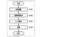
- FIG. 1 is a flowchart showing an outline of an example of an analysis method for blood coagulation according to an embodiment.
- FIG. 2 is a flowchart showing an outline of an example of a data analysis method regarding blood coagulation according to one embodiment.
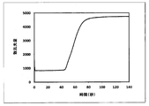
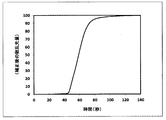
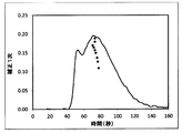
- FIG. 3 is a diagram showing an example of a coagulation reaction curve.
- FIG. 4 is a diagram showing an example of the coagulation reaction curve after the baseline adjustment.
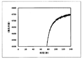
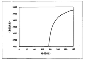
- FIG. 5A is an enlarged view of a part of an example of the coagulation reaction curve.
- FIG. 5B is an enlarged view of a part of an example of the coagulation reaction curve after the baseline adjustment.
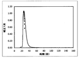
- FIG. 6 is a diagram illustrating an example of the correction-processed coagulation reaction curve.
- FIG. 1 is a flowchart showing an outline of an example of an analysis method for blood coagulation according to an embodiment.
- FIG. 2 is a flowchart showing an outline of an example of a data analysis method regarding blood coagulation according to one embodiment.
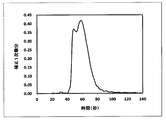
- FIG. 7 is a diagram showing an example of the corrected primary curve.
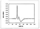
- FIG. 8 is a diagram showing an example of the corrected quadratic curve.
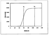
- FIG. 9 is a diagram for explaining the coagulation time, and is a diagram showing an example of the coagulation reaction curve after the baseline adjustment.
- FIG. 10A is a diagram for explaining the evaluation parameter and is a diagram showing an example of a solidification rate curve.
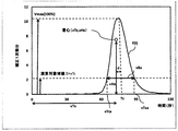
- FIG. 10B is a conceptual diagram showing the center of gravity and vTs, vTe, vB, and vW. The dotted line is a diagram showing the 10% calculation target area of the linear curve.
- FIG. 10C is a diagram showing the center of gravity of the quadratic curve.
- FIG. 10D is a conceptual diagram showing vTa, vHa, and vTm.
- the dotted line is a diagram showing the 10% calculation target area of the linear curve.
- FIG. 11 is a diagram for explaining the calculation target threshold value, the range of the corrected zero-order curve and the corrected primary curve, and the center of gravity that are the analysis targets.
- FIG. 12A is a diagram for explaining the center of gravity and the like when the calculation target range value is set to 10%.
- FIG. 12B is a diagram for explaining the center of gravity and the like when the calculation target range value is set to 80%.
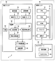
- FIG. 13 is a block diagram showing an outline of a configuration example of the automatic analyzer according to the embodiment.
- FIG. 14 is a flowchart showing an outline of an operation example of the automatic analyzer according to the embodiment.
- FIG. 15 is a flowchart showing an outline of an example of the measurement process according to the embodiment.
- FIG. 16 is a flowchart showing an outline of an example of the analysis processing according to the embodiment.
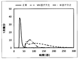
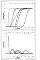
- FIG. 17A is a diagram showing an example of an uncorrected zero-order curve of normal plasma and coagulation factor-deficient plasma.
- FIG. 17B is a diagram showing an example of a corrected zero-order curve of normal plasma and coagulation factor-deficient plasma.
- FIG. 18A is a diagram showing an example of an uncorrected linear curve of normal plasma and coagulation factor-deficient plasma.
- FIG. 18B is a diagram showing an example of a corrected linear curve of normal plasma and coagulation factor-deficient plasma.
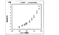
- FIG. 19A is a diagram showing an example of the relationship between the logarithm of the factor VIII concentration, the time VmaxT indicating the maximum first-order differential value, and the centroid time vT10%.
- FIG. 19B is a diagram showing an example of the relationship between the logarithm of the factor IX concentration, the time VmaxT showing the maximum first-order differential value, and the centroid time vT10%.
- FIG. 19C is a diagram showing an example of the relationship between the logarithm of the factor VIII concentration and the maximum first-order differential value Vmax and the height of the center of gravity vH60%.
- FIG. 19A is a diagram showing an example of the relationship between the logarithm of the factor VIII concentration, the time VmaxT indicating the maximum first-order differential value, and the centroid time vT10%.
- FIG. 19B is a diagram showing
- FIG. 19D is a diagram showing an example of the relationship between the logarithm of the factor IX concentration, the maximum first-order differential value Vmax, and the height of the center of gravity vH60%.
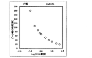
- FIG. 20A is a diagram showing an example of the relationship between the logarithm of factor VIII concentration and the peak width vB10%.
- FIG. 20B is a diagram showing an example of the relationship between the logarithm of the factor IX concentration and the peak width vB10%.
- FIG. 21A is a diagram showing the position of the center of gravity according to the calculation target range value in an example of the corrected primary curve of normal plasma.
- FIG. 21B is a diagram showing the position of the center of gravity point according to the calculation target threshold value in an example of the corrected primary curve of factor VIII-deficient plasma.
- FIG. 21C is a diagram showing the position of the center of gravity point according to the calculation target threshold value in an example of the corrected primary curve of factor IX-deficient plasma.
- FIG. 22A is a diagram showing an example of the center-of-gravity time according to the calculation target threshold value.
- FIG. 22B is a diagram showing an example of the relative difference in the centroid times according to the calculation target threshold value.
- FIG. 22C is a diagram showing an example of the height of the center of gravity according to the calculation target threshold value.
- FIG. 23 is a diagram for explaining an example of the behavior of the center of gravity depending on the calculation target threshold value that differs depending on the sample.
- FIG. 24A is a diagram showing an example of a corrected primary curve calculated based on the difference method.
- FIG. 24B is a diagram showing an example of the corrected linear curve calculated based on the average inclination in the section.
- FIG. 25A is a diagram showing an example of flatness vAB80% obtained by performing a correction process on the logarithm of the factor VIII concentration.
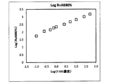
- FIG. 25B is a diagram showing an example of the flatness RvAB80% obtained without performing the correction process on the logarithm of the factor VIII concentration.
- 25C is a diagram showing an example of the logarithm of the flattening rate vAB80% obtained by performing the correction process on the logarithm of the factor VIII concentration.
- FIG. 25D is a diagram showing an example of the logarithm of the flattening rate RvAB80% obtained without performing the correction process on the logarithm of the factor VIII concentration.
- FIG. 26 is a diagram showing an example of a corrected linear curve for each factor VIII concentration.
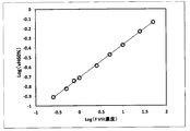
- FIG. 27 is a diagram showing an example of the relationship between the logarithm of the factor VIII concentration and the logarithm of the center of gravity height vH60%.
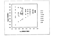
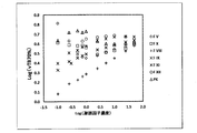
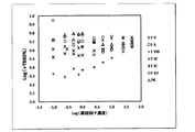
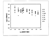
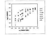
- FIG. 28A is a diagram showing an example of the relationship between the logarithm of the concentrations of various coagulation factors and the logarithm of the time rate vTB5%.
- FIG. 28B is a diagram showing an example of the relationship between the logarithm of the concentrations of various coagulation factors and the logarithm of the time rate vTB10%.
- FIG. 28C is a diagram showing an example of the relationship between the logarithm of the concentrations of various coagulation factors and the logarithm of the time rate vTB20%.
- FIG. 28D is a diagram showing an example of the relationship between the logarithm of the concentrations of various coagulation factors and the logarithm of the time rate vTB30%.
- FIG. 28E is a diagram showing an example of the relationship between the logarithm of the concentrations of various coagulation factors and the logarithm of the time rate vTB40%.
- FIG. 28F is a diagram showing an example of the relationship between the logarithm of the concentrations of various coagulation factors and the logarithm of the time rate vTB50%.
- FIG. 28G is a diagram showing an example of the relationship between the logarithm of the concentrations of various coagulation factors and the logarithm of the time rate vTB60%.
- FIG. 28H is a diagram showing an example of the relationship between the logarithm of the concentrations of various coagulation factors and the logarithm of the time rate vTB70%.
- FIG. 28I is a diagram showing an example of the relationship between the logarithm of the concentrations of various coagulation factors and the logarithm of the time rate vTB80%.
- FIG. 28J is a diagram showing an example of the relationship between the logarithm of the concentrations of various coagulation factors and the logarithm of the time rate vTB90%.
- FIG. 28K is a diagram showing an example of the relationship between the logarithm of the concentrations of various coagulation factors and the logarithm of the time rate vTB95%.
- FIG. 29 shows an example of the relationship between the factor VIII concentration and the time rate vTB for each calculation target threshold value.
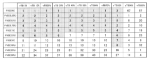
- FIG. 30 shows an example of the rank order of the time rates obtained for each concentration of factor VIII among the time rates obtained for various concentrations of coagulation factors.
- FIG. 31 shows an example of the correlation between the logarithm of the factor VIII concentration and the logarithm of the time rate.
- FIG. 32 is a diagram showing an example of the relationship of the correlation coefficient between the logarithm of the factor VIII concentration and the logarithm of the time rate obtained for each calculation target threshold value.
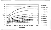
- FIG. 33 is a diagram showing an example of the relationship among the calculation target range value, the center-of-gravity height vH, and the maximum first-order differential value Vmax obtained for each factor VIII concentration.
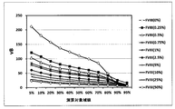
- FIG. 34 is a diagram showing an example of the relationship between the calculation target threshold value and the peak width vB obtained for each factor VIII concentration.
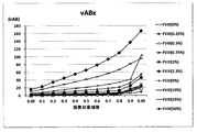
- FIG. 35A is a diagram showing an example of the relationship between the calculation target threshold value and the oblateness vAB obtained for each factor VIII concentration.
- FIG. 35B is a diagram showing an example of the relationship between the calculation target threshold value and the logarithm of the oblateness vAB obtained for each factor VIII concentration.
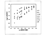
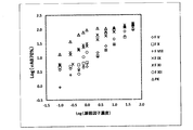
- FIG. 36A is a diagram showing an example of the relationship between the logarithm of the concentrations of various coagulation factors and the logarithm of the oblateness vAB5%.
- FIG. 35A is a diagram showing an example of the relationship between the calculation target threshold value and the peak width vB obtained for each factor VIII concentration.
- FIG. 35A is a diagram showing an example of the relationship between the calculation target threshold value and the oblateness vAB obtained for each factor VIII concentration.
- FIG. 35B is a diagram showing an
- FIG. 36B is a diagram showing an example of the relationship between the logarithm of the concentrations of various coagulation factors and the logarithm of the oblateness vAB10%.
- FIG. 36C is a diagram showing an example of the relationship between the logarithm of the concentrations of various coagulation factors and the logarithm of the oblateness vAB20%.
- FIG. 36D is a diagram showing an example of the relationship between the logarithm of the concentrations of various coagulation factors and the logarithm of the oblateness vAB30%.
- FIG. 36E is a diagram showing an example of the relationship between the logarithm of the concentrations of various coagulation factors and the logarithm of the oblateness vAB40%.
- FIG. 36F is a diagram showing an example of the relationship between the logarithm of the concentrations of various coagulation factors and the logarithm of the oblateness vAB50%.
- FIG. 36G is a diagram showing an example of the relationship between the logarithm of the concentrations of various coagulation factors and the logarithm of the oblateness vAB60%.
- FIG. 36H is a diagram showing an example of the relationship between the logarithm of the concentrations of various coagulation factors and the logarithm of the oblateness vAB70%.
- FIG. 36I is a diagram showing an example of the relationship between the logarithm of the concentrations of various coagulation factors and the logarithm of the oblateness vAB80%.
- FIG. 36J is a diagram showing an example of the relationship between the logarithm of the concentrations of various coagulation factors and the logarithm of the oblateness vAB90%.
- FIG. 36K is a diagram showing an example of the relationship between the logarithm of the concentrations of various coagulation factors and the logarithm of the oblateness vAB95%.
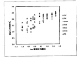
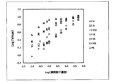
- FIG. 37A is a diagram showing an example of the relationship between the logarithms of the concentrations of various coagulation factors and the logarithm of the maximum first derivative Vmax.
- FIG. 37B is a diagram showing an example of the relationship between the logarithm of the concentrations of various coagulation factors and the logarithm of the center of gravity pH 90% of the plus peak of the corrected quadratic curve.
- FIG. 38 shows an example of the relationship between the factor VIII concentration, the flattening rate vAB and the maximum first-order differential value Vmax for each threshold value to be calculated.
- FIG. 39 shows an example of the correlation between the logarithm of the factor VIII concentration, the logarithm of the flattening rate, and the logarithm of the maximum first derivative value Vmax.
- FIG. 40 shows an example of the ratio (recovery rate) between the known concentration of Factor VIII and the calculated concentration obtained from the calibration curve using the values shown in FIG. 39.
- FIG. 41A is a diagram showing an example of an uncorrected 0th-order curve (the amount of scattered light without correction) and an uncorrected 1st-order curve of normal plasma and various plasmas lacking coagulation factors.
- FIG. 41B is a diagram showing an example of a corrected 0th-order curve and a corrected 1st-order curve of normal plasma and various clotting factor-deficient plasmas.
- FIG. 42A is a diagram showing an example of an uncorrected quadratic curve of normal plasma and plasmas lacking various coagulation factors.
- the right diagram is a diagram in which the scale in the y-axis direction of the left diagram is changed.
- FIG. 42B is a diagram showing an example of a corrected quadratic curve of normal plasma and various plasmas lacking coagulation factors.
- the right diagram is a diagram in which the scale in the y-axis direction of the left diagram is changed.
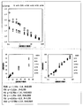
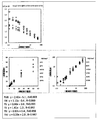
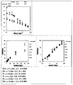
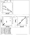
- the upper diagram of FIG. 43A is a diagram showing an example of the relationship between the logarithm of the concentrations of various coagulation factors and the logarithm of APTT.
- the middle left figure shows a plot of the calculated concentration based on the calibration curve with respect to the actual concentration of the coagulation factor.
- the middle right figure shows a logarithmic plot of the measured concentration and the calculated concentration.
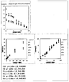
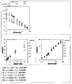
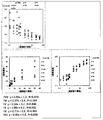
- the upper diagram of FIG. 43B is a diagram showing an example of the relationship between the logarithm of the concentrations of various coagulation factors and the logarithm of T5.
- the middle left figure shows a plot of the calculated concentration based on the calibration curve with respect to the actual concentration of the coagulation factor.
- the middle right figure shows a logarithmic plot of the measured concentration and the calculated concentration.
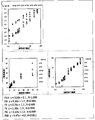
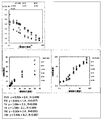
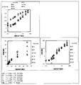
- the upper diagram of FIG. 43C is a diagram showing an example of the relationship between the logarithm of the concentrations of various coagulation factors and the logarithm of T95-T5.
- the middle left figure shows a plot of the calculated concentration based on the calibration curve with respect to the actual concentration of the coagulation factor.
- the middle right figure shows a logarithmic plot of the measured concentration and the calculated concentration.
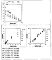
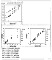
- the upper diagram of FIG. 43D is a diagram showing an example of the relationship between the logarithm of the concentrations of various coagulation factors and the logarithm of VmaxT.
- the middle left figure shows a plot of the calculated concentration based on the calibration curve with respect to the actual concentration of the coagulation factor.
- the middle right figure shows a logarithmic plot of the measured concentration and the calculated concentration.
- FIG. 43E is a diagram showing an example of the relationship between the logarithm of the concentrations of various coagulation factors and the logarithm of Vmax.
- the middle left figure shows a plot of the calculated concentration based on the calibration curve with respect to the actual concentration of the coagulation factor.
- the middle right figure shows a logarithmic plot of the measured concentration and the calculated concentration.
- the upper diagram of FIG. 43F is a diagram showing an example of the relationship between the logarithm of the concentrations of various coagulation factors and the logarithm of AmaxT.
- the middle left figure shows a plot of the calculated concentration based on the calibration curve with respect to the actual concentration of the coagulation factor.
- the middle right figure shows a logarithmic plot of the measured concentration and the calculated concentration.
- the upper diagram of FIG. 43G is a diagram showing an example of the relationship between the logarithm of the concentrations of various coagulation factors and the logarithm of Amax.
- the middle left figure shows a plot of the calculated concentration based on the calibration curve with respect to the actual concentration of the coagulation factor.
- the middle right figure shows a logarithmic plot of the measured concentration and the calculated concentration.
- the upper diagram of FIG. 43H is a diagram showing an example of the relationship between the logarithm of the concentrations of various coagulation factors and the logarithm of vAUC20%.
- the middle left figure shows a plot of the calculated concentration based on the calibration curve with respect to the actual concentration of the coagulation factor.
- the middle right figure shows a logarithmic plot of the measured concentration and the calculated concentration.
- the upper diagram of FIG. 43I is a diagram showing an example of the relationship between the logarithm of the concentrations of various coagulation factors and the logarithm of vH5%.
- the middle left figure shows a plot of the calculated concentration based on the calibration curve with respect to the actual concentration of the coagulation factor.
- the middle right figure shows a logarithmic plot of the measured concentration and the calculated concentration.
- the upper diagram of FIG. 43J is a diagram showing an example of the relationship between the logarithm of the concentrations of various coagulation factors and the logarithm of vT50%.
- the middle left figure shows a plot of the calculated concentration based on the calibration curve with respect to the actual concentration of the coagulation factor.
- the middle right figure shows a logarithmic plot of the measured concentration and the calculated concentration.
- the upper diagram of FIG. 43K is a diagram showing an example of the relationship between the logarithm of the concentrations of various coagulation factors and the logarithm of vTs50%.
- the middle left figure shows a plot of the calculated concentration based on the calibration curve with respect to the actual concentration of the coagulation factor.
- the middle right figure shows a logarithmic plot of the measured concentration and the calculated concentration.
- FIG. 43L is a diagram showing an example of the relationship between the logarithm of the concentrations of various coagulation factors and the logarithm of vTe80%.
- the middle left figure shows a plot of the calculated concentration based on the calibration curve with respect to the actual concentration of the coagulation factor.
- the middle right figure shows a logarithmic plot of the measured concentration and the calculated concentration.
- the upper diagram of FIG. 43M is a diagram showing an example of the relationship between the logarithm of the concentrations of various coagulation factors and the logarithm of vTr20%.
- the middle left figure shows a plot of the calculated concentration based on the calibration curve with respect to the actual concentration of the coagulation factor.
- the middle right figure shows a logarithmic plot of the measured concentration and the calculated concentration.
- the upper diagram of FIG. 43N is a diagram showing an example of the relationship between the logarithm of the concentrations of various coagulation factors and the logarithm of vH95% / vB95%.
- the middle left figure shows a plot of the calculated concentration based on the calibration curve with respect to the actual concentration of the coagulation factor.
- the middle right figure shows a logarithmic plot of the measured concentration and the calculated concentration.
- the upper diagram of FIG. 43O is a diagram showing an example of the relationship between the logarithm of the concentrations of various coagulation factors and the logarithm of pH 5%.
- the middle left figure shows a plot of the calculated concentration based on the calibration curve with respect to the actual concentration of the coagulation factor.
- the middle right figure shows a logarithmic plot of the measured concentration and the calculated concentration.
- the upper diagram of FIG. 43P is a diagram showing an example of the relationship between the logarithm of the concentrations of various coagulation factors and the logarithm of pT50%.
- the middle left figure shows a plot of the calculated concentration based on the calibration curve with respect to the actual concentration of the coagulation factor.
- the middle right figure shows a logarithmic plot of the measured concentration and the calculated concentration.
- FIG. 43Q is a diagram showing an example of the relationship between the logarithm of the concentrations of various coagulation factors and the logarithm of pB70%.
- the middle left figure shows a plot of the calculated concentration based on the calibration curve with respect to the actual concentration of the coagulation factor.
- the middle right figure shows a logarithmic plot of the measured concentration and the calculated concentration.
- the upper diagram of FIG. 43R is a diagram showing an example of the relationship between the logarithm of the concentrations of various coagulation factors and the logarithm of pH 5% / pB5%.
- the middle left figure shows a plot of the calculated concentration based on the calibration curve with respect to the actual concentration of the coagulation factor.
- the middle right figure shows a logarithmic plot of the measured concentration and the calculated concentration.
- the upper diagram of FIG. 43S is a diagram showing an example of the relationship between the logarithm of the concentrations of various coagulation factors and the logarithm of pAUC90%.
- the middle left figure shows a plot of the calculated concentration based on the calibration curve with respect to the actual concentration of the coagulation factor.
- the middle right figure shows a logarithmic plot of the measured concentration and the calculated concentration.
- the upper diagram of FIG. 43T is a diagram showing an example of the relationship between the logarithm of the concentrations of various coagulation factors and the logarithm of mH20%.
- the middle left figure shows a plot of the calculated concentration based on the calibration curve with respect to the actual concentration of the coagulation factor.
- the middle right figure shows a logarithmic plot of the measured concentration and the calculated concentration.
- the upper diagram of FIG. 43U is a diagram showing an example of the relationship between the logarithm of the concentrations of various coagulation factors and the logarithm of mH20% / mB20%.
- the middle left figure shows a plot of the calculated concentration based on the calibration curve with respect to the actual concentration of the coagulation factor.
- the middle right figure shows a logarithmic plot of the measured concentration and the calculated concentration.
- 43V is a diagram showing an example of the relationship between the logarithm of the concentrations of various coagulation factors and the logarithm of mAUC30%.
- the middle left figure shows a plot of the calculated concentration based on the calibration curve with respect to the actual concentration of the coagulation factor.
- the middle right figure shows a logarithmic plot of the measured concentration and the calculated concentration.
- the upper diagram of FIG. 43W is a diagram showing an example of the relationship between the logarithm of the concentrations of various coagulation factors and the logarithm of vHa50%.
- the middle left figure shows a plot of the calculated concentration based on the calibration curve with respect to the actual concentration of the coagulation factor.
- the middle right figure shows a logarithmic plot of the measured concentration and the calculated concentration.
- the upper diagram of FIG. 43X is a diagram showing an example of the relationship between the logarithm of the concentrations of various coagulation factors and the logarithm of vTm50%.
- the middle left figure shows a plot of the calculated concentration based on the calibration curve with respect to the actual concentration of the coagulation factor.
- the middle right figure shows a logarithmic plot of the measured concentration and the calculated concentration.
- the upper diagram of FIG. 43Y is a diagram showing an example of the relationship between the logarithm of the concentrations of various coagulation factors and the logarithm of RvH50% / RvB50%.
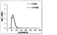
- FIG. 44A is a diagram showing corrected linear curves of LA plasma with and without heating.
- FIG. 44B is a diagram showing a corrected linear curve of Factor VIII inhibitor-positive plasma with and without heating.
- FIG. 45A is a diagram showing a corrected linear curve of a mixed plasma of LA plasma and normal plasma (LA-NP) in the non-heated state and the warmed state.
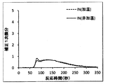
- FIG. 45B is a diagram showing a corrected primary curve of a mixed plasma (IN-NP) of factor VIII inhibitor-positive plasma and normal plasma in the non-heated state and the warmed state.
- FIG. 46A is a diagram showing a value Pa in unheated plasma, a value Pb in warmed plasma, a ratio Pa / Pb thereof, and a difference Pb-Pa regarding APTT of various plasmas.
- FIG. 46B is a diagram showing a value Pa in non-heated plasma, a value Pb in warmed plasma, a ratio Pa / Pb thereof, and a difference Pb-Pa regarding Vmax of various plasmas.
- FIG. 46C is a diagram showing a value Pa in non-heated plasma, a value Pb in warmed plasma, a ratio Pa / Pb thereof, and a difference Pb-Pa regarding Amax of various plasmas.
- FIG. 46A is a diagram showing a value Pa in unheated plasma, a value Pb in warmed plasma, a ratio Pa / Pb thereof, and a difference Pb-Pa regarding APTT of various plasmas.
- FIG. 46B is a diagram showing a value Pa in non-heated
- FIG. 46D is a diagram showing a value Pa in non-heated plasma, a value Pb in warmed plasma, a ratio Pa / Pb thereof, and a difference Pb-Pa for vB10% of various plasmas.
- FIG. 46E is a diagram showing a value Pa in unheated plasma, a value Pb in warmed plasma, a ratio Pa / Pb thereof, and a difference Pb-Pa regarding vT10% of various plasmas.
- FIG. 46F is a diagram showing a value Pa in non-heated plasma, a value Pb in warmed plasma, a ratio Pa / Pb thereof, and a difference Pb-Pa regarding vAB10% of various plasmas.
- FIG. 46G is a diagram showing a value Pa in non-heated plasma, a value Pb in warmed plasma, a ratio Pa / Pb thereof, and a difference Pb-Pa with respect to vTB10% of various plasmas.
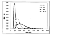
- FIG. 47A is a diagram showing a corrected primary curve of “normal plasma” when the heating time is set to 0 minutes, 10 minutes, 30 minutes, and 120 minutes, respectively.
- FIG. 47B is a diagram showing a corrected primary curve of “LA positive plasma” when the heating time is 0 minute, 10 minutes, 30 minutes, and 120 minutes, respectively.
- FIG. 47C is a diagram showing a corrected primary curve of “Factor VIII inhibitor-positive plasma” when the heating time is 0 minute, 10 minutes, 30 minutes, and 120 minutes, respectively.
- FIG. 47A is a diagram showing a corrected primary curve of “normal plasma” when the heating time is set to 0 minutes, 10 minutes, 30 minutes, and 120 minutes, respectively.
- FIG. 47B is a diagram showing a
- FIG. 47D is a diagram showing a corrected primary curve of “equal amount mixed plasma of LA-positive plasma and normal plasma” when the heating time is 0 minute, 10 minutes, 30 minutes, and 120 minutes, respectively.
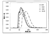
- FIG. 47E is a diagram showing a corrected linear curve of “equal volume mixed plasma of factor VIII inhibitor-positive plasma and normal plasma” when the heating time was 0 minute, 10 minutes, 30 minutes, and 120 minutes, respectively.
- FIG. 48 shows various evaluation parameters obtained from the APTT measurement data of the sample after heating for 10 minutes, various evaluation parameters obtained from the APTT measurement data of the sample without heating treatment, and It is a figure which shows an example of the table which shows the result of having calculated the ratio of both various evaluation parameters.
- FIG. 48 shows various evaluation parameters obtained from the APTT measurement data of the sample after heating for 10 minutes, various evaluation parameters obtained from the APTT measurement data of the sample without heating treatment, and It is a figure which shows an example of the table which shows the result of having calculated the ratio of both various evaluation parameters.
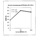
- FIG. 49A is a diagram showing the results of a cross-mixing test relating to sample A of LA-positive plasma that has not been heated and has been heated at 37 ° C. for 10 minutes.
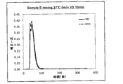
- FIG. 49B is a diagram showing the results of a cross-mixing test relating to LA-positive plasma sample B without heating and after heating at 37 ° C. for 10 minutes.
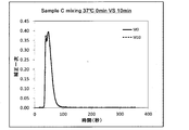
- FIG. 49C is a diagram showing the results of a cross-mixing test relating to sample C of LA-positive plasma that has not been heated and has been heated at 37 ° C. for 10 minutes.
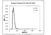
- FIG. 49D is a diagram showing the results of a cross-mixing test relating to sample D of LA-positive plasma that was not heated and was heated at 37 ° C. for 10 minutes.
- FIG. 49A is a diagram showing the results of a cross-mixing test relating to sample A of LA-positive plasma that has not been heated and has been heated at 37 ° C. for 10 minutes.
- FIG. 49B is a diagram showing the results
- FIG. 49E is a diagram showing the results of a cross-mixing test relating to sample H of LA-positive plasma that was not heated and was heated at 37 ° C. for 10 minutes.
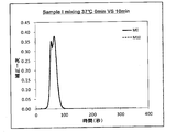
- FIG. 49F is a diagram showing the results of a cross-mixing test relating to sample I of LA-positive plasma that has not been heated and has been heated at 37 ° C. for 10 minutes.
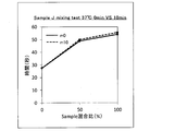
- FIG. 49G is a diagram showing the results of a cross-mixing test relating to sample J of LA-positive plasma that has not been heated and has been heated at 37 ° C. for 10 minutes.
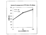
- FIG. 49H is a diagram showing the results of a cross-mixing test relating to sample K of LA-positive plasma that has not been heated and that has been heated at 37 ° C. for 10 minutes.
- FIG. 49I is a diagram showing the results of a cross-mixing test relating to sample O of LA-positive plasma after no heating treatment and after heating at 37 ° C. for 10 minutes.
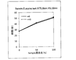
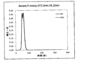
- FIG. 49J is a diagram showing a result of a cross-mixing test relating to a sample P of LA-positive plasma without heating and after heating at 37 ° C. for 10 minutes.
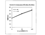
- FIG. 49K is a diagram showing the results of a cross-mixing test involving sample Q of LA-positive plasma that has not been heated and that has been heated at 37 ° C. for 10 minutes.
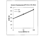
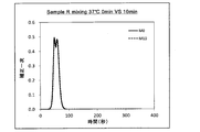
- FIG. 49L is a diagram showing the results of a cross-mixing test relating to sample R of LA-positive plasma that has not been heated and has been heated at 37 ° C. for 10 minutes.
- FIG. 49I is a diagram showing the results of a cross-mixing test relating to sample O of LA-positive plasma after no heating treatment and after heating at 37 ° C. for 10 minutes.
- FIG. 49J is a diagram showing
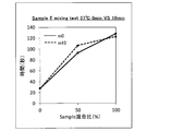
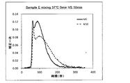
- FIG. 50A is a diagram showing the results of a cross-mixing test involving Sample E of Factor VIII inhibitor-positive plasma that has not been heated and has been heated at 37 ° C. for 10 minutes.
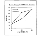
- FIG. 50B is a diagram showing the results of a cross-mixing test involving Sample F of Factor VIII inhibitor-positive plasma that has not been heated and has been heated at 37 ° C. for 10 minutes.
- FIG. 50C is a diagram showing the results of a cross-mixing test involving Sample G of Factor VIII inhibitor-positive plasma that was not heated and was heated at 37 ° C. for 10 minutes.
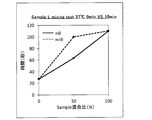
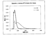
- FIG. 50D is a diagram showing the results of a cross-mixing test involving Sample L of Factor VIII inhibitor-positive plasma, which was not heated and was heated at 37 ° C.
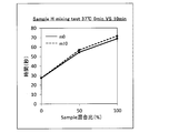
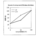
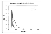
- FIG. 50E is a diagram showing the results of a cross-mixing test involving Sample M of Factor VIII inhibitor-positive plasma that has not been heated and has been heated at 37 ° C. for 10 minutes.
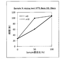
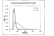
- FIG. 50F is a diagram showing the results of a cross-mixing test involving Sample N of Factor VIII inhibitor-positive plasma that has not been heated and has been heated at 37 ° C. for 10 minutes.
- FIG. 50G is a diagram showing the results of a cross-mixing test involving Sample S of Factor VIII inhibitor-positive plasma that has not been heated and has been heated at 37 ° C. for 10 minutes.
- FIG. 50E is a diagram showing the results of a cross-mixing test involving Sample M of Factor VIII inhibitor-positive plasma that has not been heated and has been heated at 37 ° C. for 10 minutes.
- FIG. 50F is a diagram showing the results of a cross-mixing test involving Sample N of Factor VIII inhibitor-positive plasma that has not been heated and has been heated at 37 ° C.
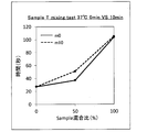
- FIG. 50H is a diagram showing the results of a cross-mixing test involving Sample T of Factor VIII inhibitor-positive plasma that was not heated and after being heated at 37 ° C. for 10 minutes.
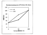
- FIG. 50I is a diagram showing the results of a cross-mixing test involving Sample U of factor VIII inhibitor-positive plasma that has not been heated and has been heated at 37 ° C. for 10 minutes.
- FIG. 51A is a diagram showing an example of APTT without heating treatment of a test plasma (single body) of each sample and after heating treatment at 37 ° C. for 10 minutes.
- FIG. 51B is a diagram showing an example of APTT without heating treatment of a mixed plasma of test plasma and normal plasma of each sample and after heating treatment at 37 ° C. for 10 minutes.
- FIG. 52A is a diagram showing an example of a corrected linear curve without heating treatment of an equal amount mixed plasma of LA-positive plasma sample A and normal plasma and after heating treatment at 37 ° C. for 10 minutes.
- FIG. 52B is a diagram showing an example of a corrected primary curve without heating treatment of an equal amount mixed plasma of LA-positive plasma sample B and normal plasma and after heating treatment at 37 ° C. for 10 minutes.
- FIG. 52C is a diagram showing an example of a corrected linear curve without heating treatment of an equal amount mixed plasma of LA-positive plasma sample C and normal plasma and after heating treatment at 37 ° C. for 10 minutes.
- FIG. 52A is a diagram showing an example of a corrected linear curve without heating treatment of an equal amount mixed plasma of LA-positive plasma sample A and normal plasma and after heating treatment at 37 ° C. for 10 minutes.
- FIG. 52D is a diagram showing an example of a corrected linear curve without heating treatment of an equal amount mixed plasma of LA-positive plasma sample D and normal plasma and after heating treatment at 37 ° C. for 10 minutes.
- FIG. 52E is a diagram showing an example of a corrected linear curve after heating treatment of equal volume mixed plasma of LA-positive plasma sample H and normal plasma without heating treatment and at 37 ° C. for 10 minutes.
- FIG. 52F is a diagram showing an example of a corrected linear curve after heating treatment of an equal amount mixed plasma of LA-positive plasma sample I and normal plasma without heating treatment and at 37 ° C. for 10 minutes.
- FIG. 52G is a diagram showing an example of a corrected linear curve after heating treatment of an equal amount mixed plasma of LA-positive plasma sample J and normal plasma without heating and at 37 ° C.
- FIG. 52H is a diagram showing an example of a corrected linear curve after heating treatment of equal amount mixed plasma of LA-positive plasma sample K and normal plasma without heating treatment and at 37 ° C. for 10 minutes.
- FIG. 52I is a diagram showing an example of a corrected linear curve after heating treatment of equal amount mixed plasma of sample O of LA positive plasma and normal plasma and after heating treatment at 37 ° C. for 10 minutes.
- FIG. 52J is a diagram showing an example of a corrected linear curve without heating treatment of an equal amount mixed plasma of LA-positive plasma sample P and normal plasma and after heating treatment at 37 ° C. for 10 minutes.
- FIG. 52H is a diagram showing an example of a corrected linear curve after heating treatment of equal amount mixed plasma of LA-positive plasma sample K and normal plasma without heating treatment and at 37 ° C. for 10 minutes.
- FIG. 52I is a diagram showing an example of a corrected linear curve after heating treatment of equal amount mixed plasma of sample O of LA positive plasma and normal plasma and after heating treatment at 37 ° C. for 10 minutes.
- 52K is a diagram showing an example of a corrected linear curve after heating treatment of an equal amount mixed plasma of LA-positive plasma sample Q and normal plasma without heating treatment and at 37 ° C. for 10 minutes.
- FIG. 52L is a diagram showing an example of a corrected linear curve without heating treatment of an equal volume mixed plasma of LA-positive plasma sample R and normal plasma and after heating treatment at 37 ° C. for 10 minutes.
- FIG. 53A is a diagram showing an example of a corrected linear curve without heating treatment of an equal amount mixed plasma of sample E of factor VIII inhibitor-positive plasma and normal plasma and after heating treatment at 37 ° C. for 10 minutes.
- FIG. 53B is a diagram showing an example of a corrected linear curve after heating treatment of an equal amount mixed plasma of sample F of factor VIII inhibitor positive plasma and normal plasma after heating treatment at 37 ° C. for 10 minutes.
- FIG. 53C is a diagram showing an example of a corrected primary curve without heating treatment of an equal amount mixed plasma of sample G of factor VIII inhibitor-positive plasma and normal plasma and after heating treatment at 37 ° C. for 10 minutes.
- FIG. 53D is a diagram showing an example of a corrected linear curve without heating treatment of an equal volume mixed plasma of Factor L inhibitor positive plasma sample L and normal plasma and after heating treatment at 37 ° C. for 10 minutes.
- FIG. 53E is a diagram showing an example of a corrected linear curve of a sample M of factor VIII inhibitor-positive plasma, which is not subjected to heating treatment of plasma mixed with an equal amount of normal plasma and after heating for 10 minutes at 37 ° C.
- FIG. 53F is a diagram showing an example of a corrected linear curve after heating treatment of an equal amount mixed plasma of sample N of factor VIII inhibitor-positive plasma and normal plasma without heating treatment and at 37 ° C. for 10 minutes.
- FIG. 53G is a diagram showing an example of a corrected linear curve of a sample S of factor VIII inhibitor-positive plasma that has not been heated and is heated at 37 ° C. for 10 minutes without heating the plasma in an equal amount.
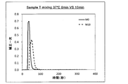
- FIG. 53H is a diagram showing an example of a corrected linear curve after heating treatment of an equal amount mixed plasma of sample T of factor VIII inhibitor-positive plasma and normal plasma and after heating treatment at 37 ° C. for 10 minutes.
- FIG. 53I is a diagram showing an example of a corrected linear curve of a sample U of factor VIII inhibitor-positive plasma, which is not subjected to heating treatment of plasma mixed with an equal amount of normal plasma and after heating for 10 minutes at 37 ° C.
- FIG. 54A shows the results of “flattening rate when the calculation target range value S is 10%” related to an equal mixture plasma of individual samples of LA-positive plasma and normal plasma, without heating treatment and after 10 minutes heating treatment.
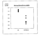
- FIG. 54B shows a heating process of “height of center of gravity when the calculation target range value S is 60%” and a heating process for 10 minutes, which relates to an equal amount mixed plasma of individual samples of LA-positive plasma and normal plasma.
- FIG. 55A shows the "flattening rate when the calculation target threshold value S is 10%" relating to an equal amount mixed plasma of individual samples of LA-positive plasma and normal plasma, without heating treatment and after 10 minutes heating treatment.
- FIG. 55B is a heating process without heating treatment and a 10-minute heating process for “height of the center of gravity when the calculation target range value S is 60%” relating to an equal amount mixed plasma of individual samples of LA-positive plasma and normal plasma.
- FIG. 55C is a graph of "centroid time when the calculation target range value S is 60%" relating to an equal amount mixed plasma of individual samples of LA-positive plasma and normal plasma, without heating treatment and after 10 minutes heating treatment.
- FIG. 56 is a diagram showing the results of a cross-mixing test relating to a sample of LA-positive plasma that has not been heated and that has been heated at 37 ° C. for 2 minutes.
- FIG. 57 is a diagram showing the results of a cross-mixing test relating to LA-positive plasma samples after heating at 37 ° C. for 2 minutes and after heating for 10 minutes.
- FIG. 58 is a diagram showing the results of a cross-mixing test involving samples of Factor VIII inhibitor-positive plasma that were not heated and were heated at 37 ° C. for 2 minutes.
- FIG. 59 is a diagram showing the results of a cross-mixing test involving samples of Factor VIII inhibitor-positive plasma after heating at 37 ° C. for 2 minutes and after heating for 10 minutes.
- FIG. 60 is a diagram showing an example of a corrected linear curve without heating treatment of an equal amount mixed plasma of LA positive plasma sample and normal plasma and after heating treatment at 37 ° C. for 2 minutes.
- FIG. 61 is a diagram showing an example of a corrected linear curve after heating treatment of equal volume mixed plasma of a sample of factor VIII inhibitor positive plasma and normal plasma without heating treatment and after heating treatment at 37 ° C.
- FIG. 62 shows various evaluation parameters obtained from APTT measurement data of a sample after heating for 2 minutes, various evaluation parameters obtained from APTT measurement data of a sample without heating treatment, and It is a figure which shows an example of the table which shows the result of having calculated the ratio of both various evaluation parameters.
- FIG. 63A is a diagram showing a difference (Pb-Pa) and a ratio (Pb / Pa) between unheated plasma and warmed plasma with respect to APTT time (T50) and Vmax of mixed plasma.
- LA Mixed plasma of LA positive plasma and normal plasma
- Inhibitor Mixed plasma of factor VIII inhibitor positive plasma and normal plasma.
- FIG. 63B is a diagram showing the difference (Pb-Pa) and the ratio (Pb / Pa) between non-warmed plasma and warmed plasma for vAB40% and vABa40% of mixed plasma (LA and Inhibitor).
- FIG. 63C is a diagram showing a difference (Pb-Pa) and a ratio (Pb / Pa) between unheated plasma and heated plasma for vH40% and vHa40% of mixed plasma (LA and Inhibitor).
- FIG. 63D is a diagram showing a difference (Pb-Pa) and a ratio (Pb / Pa) between unheated plasma and warmed plasma for vAUC90% and vW10% / vB10% of mixed plasma (LA and Inhibitor).
- FIG. 63E is a diagram showing a difference (Pb-Pa) and a ratio (Pb / Pa) between unheated plasma and warmed plasma for pAUC80% and mAUC20% of mixed plasma (LA and Inhibitor).
- the present invention relates to a method for analyzing coagulation characteristics of a blood sample by applying waveform analysis.
- the present invention also relates to shortening the test time of the blood coagulation test.
- the present invention excellent analysis of the coagulation characteristics of a blood sample can be realized.
- the inspection time of the cross mixing test can be shortened.
- the heating time can be shorter than 2 hours, for example, 10 minutes.
- the present embodiments relate to analyzing the properties of analytes associated with blood coagulation.
- the activated partial thromboplastin time (APTT) measurement used for the examination of intrinsic coagulation function is performed and the obtained data is analyzed. It can be similarly applied to analysis of data obtained by measurement of other test items using a coagulation reaction curve including prothrombin time (PT) used for testing extrinsic coagulation function.
- APTT activated partial thromboplastin time
- PT prothrombin time
- Analysis method 1.1 Outline of Analysis Method
- the outline of the analysis method according to the present embodiment will be described with reference to the flowchart shown in FIG.
- a sample used for the inspection is prepared (step S101).
- the coagulation time is measured for the prepared sample (step S102). Examples of measurement of coagulation time include measurement of APTT and PT.
- a predetermined analysis is performed on the data obtained by measuring the coagulation time (step S103).
- the blood coagulation function of the sample is evaluated based on the analysis result (step S104).
- sample Preparation and Coagulation Time Measurement The sample preparation performed in step S101 and the coagulation time measurement performed in step S102 will be described. Here, the measurement of the coagulation time will be described by taking the measurement of APTT as an example.
- the sample to be tested is, for example, a blood sample derived from a subject who is required to test for abnormalities caused by coagulation factors. More specifically, the blood plasma of a subject is used as the blood sample.
- a well-known anticoagulant usually used for a coagulation test may be added to the blood sample.
- blood can be collected using a blood collection tube containing sodium citrate, and plasma can be immediately centrifuged.
- a contact factor activator and phospholipid are added to the test plasma.
- the activator ellagic acid, celite, kaolin, silica, polyphenol compound and the like can be used.
- animal-derived, plant-derived, or synthetic-derived phospholipid is used. Examples of animal-derived phospholipids include those derived from rabbit brain, chicken, and pig. Examples of plant-derived phospholipids include those derived from soybean. Further, a buffer solution such as Tris-hydrochloric acid may be appropriately added.
- APTT In order to measure APTT, a commercially available APTT measurement reagent, a reagent kit, or the like can be used.
- APTT-N manufactured by Sekisui Medical Co., Ltd.
- Coagpia APTT-N manufactured by Sekisui Medical Co., Ltd.
- the sample in which the activator and phospholipid are added to the above-mentioned test plasma is heated and the contact factor in the plasma is activated.
- the temperature condition is, for example, 30 ° C. or higher and 40 ° C. or lower, preferably 35 ° C. or higher and 39 ° C. or lower.
- the coagulation reaction of the mixed solution after addition of the calcium chloride solution can be measured.
- an optical method of measuring the scattered light amount of light or the transmittance (or absorbance) may be used, or a mechanical method of measuring the viscosity of plasma may be used.
- the measured time is, for example, several tens of seconds to 5 minutes, starting from the timing of adding the final reagent. During this period, the measurement is repeatedly performed, for example, periodically. For example, if it is an optical method, photometry may be performed at a cycle of 0.1 second.
- the time when the calcium chloride solution is added can be set as the reaction start time. Other timings may be defined as the reaction start time.
- the temperature condition during measurement is, for example, 30 ° C. or higher and 40 ° C. or lower, and preferably 35 ° C. or higher and 39 ° C. or lower.
- the above measurement may be performed using a device that can automatically perform a series of measurements.
- An example of such an apparatus is an automatic blood coagulation analyzer CP3000 (manufactured by Sekisui Medical Co., Ltd.).
- some operations may be performed manually.
- the sample may be prepared manually and the measurement may be carried out by an optical analyzer.
- various conditions can be set appropriately depending on the mixing method and the measuring method.
- FIG. 2 is a flowchart showing an outline of data analysis.
- step S201 the data to be analyzed is acquired.
- This data is data obtained by blood coagulation measurement, for example, data reflecting the coagulation reaction process obtained by APTT measurement described above.
- a calcium chloride solution is added to a sample in which an activator and a phospholipid are added to test plasma, and data showing the time change of the scattered light amount after that is acquired.
- the data analysis may be performed immediately after the measurement, or may be performed later on the data measured and stored in advance.
- Fig. 3 shows an example of the acquired data.
- the horizontal axis represents the elapsed time after the calcium chloride solution was added
- the vertical axis represents the scattered light amount. Since the coagulation reaction of the mixed solution proceeds with the passage of time, the amount of scattered light increases. In the present embodiment, such a curve indicating the time change of the measured light amount will be referred to as a coagulation reaction curve.
- the example shown in Fig. 3 is the measurement result of the scattered light amount, and the coagulation reaction curve has a sigmoid shape, but when the transmitted light amount is measured, the coagulation reaction curve has an inverse sigmoid shape.
- the case where the scattered light amount is measured is shown as an example, but the same process can be performed when the transmitted light amount and the absorbance are measured.
- Data indicating the amount of coagulation reaction obtained by other methods, including the method of obtaining the coagulation reaction curve by the change in viscosity of the mixed liquid, may be analyzed.
- the baseline adjustment includes smoothing processing and zero point adjustment.
- FIG. 4 shows an example of data after performing the baseline adjustment on the data shown in FIG.
- FIG. 5A shows an enlarged view of the data before the baseline adjustment shown in FIG.
- FIG. 5B shows an enlarged view of the data after the baseline adjustment shown in FIG.
- smoothing processing including noise removal is performed in the baseline adjustment.
- any of various known methods for noise removal can be used.
- the amount of scattered light at the start of measurement is larger than zero. This is because the mixed solution containing the test plasma originally scatters light. In the baseline adjustment, the amount of scattered light at the start of measurement is adjusted to 0 as shown in FIG.
- step S203 correction processing is performed on the data after the baseline adjustment.
- the correction is performed so that the maximum value of the coagulation reaction curve after the baseline adjustment becomes 100.
- FIG. 6 shows the result of performing the correction process on the data shown in FIG.
- the coagulation reaction curve after the baseline adjustment will be expressed as D (t).
- the maximum value of D (t) is Dmax
- the minimum value of D (t) is Dmin.
- the change width of D (t), that is, Dmax-Dmin is set as Drange.
- P (t) [(D (t) -Dmin) / Drange] ⁇ 100 (1)
- the coagulation reaction curve obtained from the corrected data will be referred to as the corrected coagulation reaction curve.
- the purpose of this correction processing is as follows.
- the height of the coagulation reaction curve after the baseline adjustment depends on the fibrinogen concentration of the sample. Fibrinogen levels vary from individual to individual and can vary from sample to sample.
- the coagulation waveform parameter that does not depend on the fibrinogen concentration can be obtained. That is, with this correction, it becomes possible to quantitatively compare the difference in the shape of the coagulation reaction curve after the baseline adjustment between the samples. It should be noted that although the value after correction is corrected here to be 0 to 100, other values may be used. Further, this correction process does not necessarily have to be performed.
- step S204 a differential curve obtained by differentiating the coagulation reaction curve is calculated.
- FIG. 7 shows a first derivative curve obtained by performing a process corresponding to the first derivative on the corrected coagulation reaction curve shown in FIG. 6. The method of calculating the first derivative curve will be described in detail later.
- the first derivative of the corrected coagulation reaction curve (corrected first derivative) is the change width per time when the total reaction change width is 100, and can be called the coagulation reaction progress rate (coagulation progress rate).
- the coagulation progress rate is 100 when integrated over the entire area.
- the first-order derivative of the coagulation reaction curve that has not been subjected to the correction process indicates the value of the actually measured reaction change width per unit time, which indicates the coagulation rate.
- the second derivative curve as shown in FIG. 8 may be obtained by further differentiating the first derivative curve of the corrected coagulation reaction curve shown in FIG. 7. Further, the second derivative curve indicating the coagulation acceleration may be acquired by further differentiating the first derivative curve of the coagulation reaction curve without the correction process.
- the correction-processed coagulation reaction curve and the correction-free coagulation reaction curve are also referred to as a corrected 0th-order curve and an uncorrected 0th-order curve, respectively, and are collectively referred to as a “0th-order curve”. Also called.
- the first-order differential curves of the corrected zero-order curve and the uncorrected zero-order curve are referred to as a corrected first-order curve and an uncorrected first-order curve, respectively, and are collectively referred to as “1. It is also called the "second curve".
- the second derivative curve of the corrected zero-order curve and the uncorrected zero-order curve, or the corrected first-order curve and the first-order derivative curve of the uncorrected first-order curve are respectively corrected by It is also called a secondary curve and an uncorrected quadratic curve, and these are also collectively referred to as a “quadratic curve”.
- the coagulation progress rate, the coagulation rate, and other values indicating the progress of coagulation are collectively referred to as the first-order differential value.
- the matters described by taking the rate of coagulation progress or the rate of coagulation as an example can be similarly applied to the general first derivative.
- values representing the rate of change of coagulation acceleration and other primary differential values are collectively referred to as secondary differential values.
- step S205 various evaluation parameters are calculated.
- the evaluation parameter is a parameter indicating the blood coagulation characteristic of the sample. The evaluation parameters will be described later in detail.
- the coagulation reaction curve of the abnormal coagulation sample in which the coagulation time is remarkably delayed becomes gentler than that of the normal sample, and the shape of the coagulation reaction curve at the end of the reaction also becomes a gentle plateau.
- the difference between A (n) and A (n-1) is small, the value of B (n) becomes small even near the maximum value of the linear curve.
- Such a state is a state in which the S / N ratio is deteriorated and is easily affected by noise in numerical calculation, and the information due to the coagulation reaction is easily buried in the noise.
- the calculation result of the first derivative using the above equation (2) may be a discrete value.
- the blood coagulation reaction curve obtained by photometry performed every 0.1 seconds consider obtaining the first-order differential value for the n-th value as the difference value between the n-th value and the (n-1) th value. .
- the obtained first derivative curve may have discrete values.
- the fibrinogen concentration is low
- the height of the coagulation reaction curve is low.
- One possible solution is to shorten the measurement time interval and increase the measurement sensitivity. However, shortening the measurement time interval may increase the cost of the apparatus and may not be preferable.
- An average slope value is obtained for each measurement point N in the coagulation reaction curve that has not been subjected to correction processing or has been subjected to correction processing.
- Measurement data within a certain period of time can be used to calculate the average slope value. That is, a certain number of measurement data before and after each measurement point N, for example, 2K + 1 measurement data from N ⁇ K to N + K can be used. For example, N-2, N-1, N, N + 1, N + 2 5th measurement data can be utilized.
- the average slope value means a slope value when these plural measurement points are linearly approximated.
- a well-known method such as the least square method can be used for the calculation method of the linear approximation.
- the average slope value of these measurement data can be regarded as the first derivative value at the measurement point N.
- the average slope a within the section is expressed by the following equation (4).
- the intra-section average slope a can be calculated.
- evaluation parameters are calculated based on the 0th-order curve, the 1st-order curve, and the 2nd-order curve. The parameters will be described.
- the coagulation time which is one of the evaluation parameters of the present embodiment, will be described with reference to the coagulation reaction curve after the baseline adjustment shown in FIG.
- the point at which the amount of change in the scattered light amount in the coagulation reaction curve after the baseline adjustment satisfies a predetermined condition is set as the coagulation end determination point Te.
- the point at which the amount of change in the scattered light amount per unit time becomes equal to or less than a predetermined value is set as the solidification end determination point Te.
- the reaction elapsed time corresponding to the amount of scattered light c% is defined as the solidification time Tc.
- the reaction elapsed time corresponding to a scattered light amount of 50% is set as the coagulation time T50.
- Tc the coagulation time Tc
- the method for determining the coagulation time Tc is not limited to this method. Clotting time may be defined by other methods. For example, the time at which the coagulation rate becomes maximum may be set as the coagulation time, or the reaction elapsed time T50 at which the corrected scattered light amount becomes 50% as shown in FIG. 6 may be set as the coagulation time Tc.
- FIG. 10A shows an example of the corrected linear curve.
- the maximum value Vmax of the corrected first derivative (coagulation progress rate) can also be an evaluation parameter.
- the corrected linear curve is taken as an example, but the same applies to an uncorrected linear curve.
- the maximum value of the solidification rate can also be an evaluation parameter.
- the value of this S is the calculation target range.
- the value will be referred to as S (%).
- the calculation target threshold value S can be set to limit the peak range that reflects the characteristics of the peak shape of the linear curve. In order to limit the peak shape relatively widely, the calculation target threshold value S can be set to 5% to 20%. When the calculation target threshold value S is increased, the influence of the upper shape of the peak is relatively reflected in the analysis result. In order to analyze the shape of the upper part of the peak, the calculation target threshold value S can be set to 20% to 95%.
- the calculation target threshold value S can be similarly applied to the solidification rate curve.
- the threshold value S to be calculated can also be applied to a quadratic curve. As shown in FIG. 8, the quadratic curve has peaks in both the plus and minus directions.
- the calculation target threshold value S can be set for each of the plus peak and the minus peak of the quadratic curve.
- the time indicating the center of gravity is the center of gravity time vT. That is, the centroid time vT of the primary curve is the time from the reaction start time to the centroid, and is the x coordinate of the centroid in the graph as shown in FIG. 10A.
- the primary differential value indicating the center of gravity is defined as the center of gravity height vH. That is, the height vH of the center of gravity of the primary curve is the y coordinate of the center of gravity in the graph as shown in FIG. 10A.
- the center of gravity time vT and the center of gravity height vH are obtained as follows.
- the integrated value M is represented by the following formula (5).
- the center of gravity point, the center of gravity time vT, and the center of gravity height vH can be defined in the same manner. .. That is, the barycentric point, the barycentric time vT, and the barycentric height vH can be defined for the primary differential values including the coagulation rate and the corrected primary differential.
- the center of gravity time vT and the center of gravity height vH can be evaluation parameters.
- the t2 may be referred to as a region start time vTs and a region end time vTe (vTs ⁇ vTe), respectively (FIG. 10A).
- FIG. 11 shows the relationship between the calculation target threshold value S, the range of the corrected 0th-order curve and the corrected 1st-order curve to be analyzed at that time, and the obtained center-of-gravity point for certain data.
- the upper row, the interruption, and the lower row show the cases where the calculation target threshold value S is 10%, 50%, and 80%, respectively.
- the left column shows the corrected 0th-order curve
- the right column shows the corrected 1st-order curve and the center of gravity. The position of the center of gravity changes as shown in FIG. 11 along with the change of the calculation target threshold value S.
- the center of gravity point, the center of gravity time, and the center of gravity height can be defined for the quadratic curve.
- the time t [t1, ..., t2] (t1 ⁇ t2) is calculated, and the positive peak centroid time pT and the centroid height pH are calculated according to the above equations (5) to (7).
- the position of the center of gravity changes as the calculation target threshold value S changes.
- the minimum value and the maximum value of the reaction time at which the second derivative value at the plus peak of the quadratic curve is equal to or more than the threshold value S to be calculated are pTs and pTe, respectively, and F'in the time from pTs to pTe.
- the peak width pB of the quadratic curve is the time length of (t) ⁇ S (value obtained by subtracting 1 from the number of data points of F ′ (t) ⁇ S multiplied by the photometric time interval).
- the minimum value and the maximum value of the reaction time at which the secondary differential value at the negative peak of the quadratic curve is less than or equal to the calculation target threshold value S are mTs and mTe, respectively, and F'in the time from mTs to mTe.
- the peak width mB of the negative peak of the quadratic curve is the time length of (t) ⁇ S (value obtained by subtracting 1 from the number of data points of F ′ (t) ⁇ S multiplied by the photometric time interval).
- a further example of the parameter used in the present invention is the barycentric peak width vW.
- vW is the peak width that satisfies the primary curve F (t) ⁇ vH (the time that F (t) ⁇ vH is satisfied from the minimum time to the maximum time that satisfies F (t) ⁇ vH. Long).
- vTr is the width from vTs to vTe.
- FIG. 10B shows the calculation target range (dotted line) of the linear curve when the calculation target range value S is 10%.
- the center of gravity (vT, vH) black circles), vTs, and vTe are shown at the top of FIG.
- FIG. 10B shows the peak width satisfying F ′ (t) ⁇ pH.
- the peak width satisfying F ′ (t) ⁇ pH is defined as the barycentric peak width pW.
- the width of the coagulation reaction time that satisfies F ′ (t) ⁇ mH is defined as the barycentric peak width mW.
- FIG. 10C shows the positive peak centroid (pT, pH) and the negative peak centroid (mT, mH) of the quadratic curve when the calculation target threshold value S is 10%.
- parameters used in the present invention include average time vTa, average height vHa, and area central time vTm.
- FIG. 10D the average point (vTa, vHa) (white diamond), the center of gravity (vT, vH) (black circle), vTs, vTe, and vTm of the linear curve when the target threshold S is 10%. It is shown.
- vTa, vHa, and vTm are respectively expressed by the following equations when the number of data points from F (vTs) to F (vTe) is n.
- the area center time vTm for the plus and minus peaks of the quadratic curve can be obtained.
- the flatnesses vAB, vABa, and the center-of-gravity peak width based on the peak width of the primary curve are used.
- the flattening ratios vAW and vAWa based on are defined as in the following formulas (8a), (8b), (8c), and (8d).
- vAB vH / vB (8a)
- vAW vH / vW (8b)
- vABa vHa / vB (8c)
- vAWa vHa / vW (8d)
- the time ratio vTB based on the peak width of the primary curve and the time ratio vTW based on the barycentric peak width are given below using the barycentric time vT, the peak width vB, and the barycentric peak width vW of the primary curve. It is defined as in equations (9a) and (9b).
- vTB vT / vB (9a)
- vTW vT / vW (9b)
- vAB (vH / vB) K
- vAB (vB / vH) K
- vAW (vH / vW) K
- vAW (vW / vH) K
- vABa (vHa / vB) K
- vABa (vB / vHa) K
- vAWa (vHa / vW) K
- vAWa (vW / vHa) K
- vTB (vB / vT) K
- vTW (vT / vW) K
- vTW (vW / vT) K.
- peak width vB, center of gravity peak width vW, average time vTa, average height vHa, region start time vTs, region end time vTe, region center time vTm, peak width vTr, flatness vAB, vAW, vABa, vAWa and time rates vTB and vTW are also parameters related to the center of gravity and can be evaluation parameters in the present invention.
- the flatness ratio and time ratio as described above can be obtained for a quadratic curve.
- the flatness pAB based on the peak width or the flatness pAW based on the center of gravity peak width can be obtained as the ratio of pH to pB or pW, while pT and pB or As a ratio with pW, the time rate pTB based on the peak width or the time rate pTW based on the center-of-gravity peak width can be obtained.
- the flatness mAB based on the peak width or the flatness mAW based on the center-of-gravity peak width can be obtained as the ratio of mH and mB or mW, while mT and mB
- the time rate mTB based on the peak width or the time rate mTW based on the center-of-gravity peak width can be obtained as a ratio with mW.
- each parameter may be displayed with the calculation target range value S from which it is derived.
- the parameters related to the center of gravity of the primary curve when S is x (%) may be referred to as vHx, vTx, vBx, vWx and the like.
- the parameters vH, vT, vB, vW, vTa, vHa, vTs, vTe, vTm, vTr, vAB, vAW, vABa, vAWa, vTB, vTW related to the center of gravity of the linear curve when S is 10%.
- 12A and 12B show each parameter when the calculation target range value S is different for the same linear curve.
- 12A shows the case where the calculation target range value S is 10%
- FIG. 12B shows the case where the calculation target range value S is 80%.
- the centroid height vH10% of the primary curve is 0.4
- the centroid time vT10% is 149 seconds
- the peak width vB10% is 200 seconds.
- the center of gravity height vH80% is 0.72
- the center of gravity time vT80% is 119 seconds
- the peak width vB80% is 78 seconds. ..
- AUC area under the curve
- PAUC AUC
- mAUC AUC
- vAUC, pAUC, and mAUC in the calculation target area where S is 5% are vAUC5%, pAUC5%, and mAUC5%, respectively.
- further parameters other than the parameters related to the center of gravity described above may be included in the parameters used in the present invention.
- the parameters include the above-mentioned coagulation time Tc, maximum first-order differential value Vmax, maximum second-order differential value Amax, minimum second-order differential value Amin, and VmaxT, AmaxT, AminT representing the time to reach them. Be done. These parameters can also be used as evaluation parameters.
- the series of parameters described above may include a parameter derived from a corrected coagulation reaction curve (corrected 0th to quadratic curve) and a parameter derived from an uncorrected coagulation reaction curve (uncorrected 0th to 2nd curve).
- the barycentric time, barycentric height, peak width, average time, average height, flattening ratio, time ratio, and AUC of the primary and quadratic curves are determined by setting the calculation target threshold value S.
- the reflection result of the characteristics regarding may change.
- the combination of the above parameters may reflect the characteristics related to blood coagulation.
- the results of the four arithmetic operations of these parameters and other various operations may more significantly reflect the characteristics relating to blood coagulation.
- coagulation time Tc center of gravity time vT, center of gravity height vH, peak width vB, center of gravity peak width vW, average time vTa, average height vHa, flatness vAB and vAW, vABa, vAWa, hour rate vTB or vTW, or Based on vAUC, or a combination thereof, coagulation factor deficiency status, presence of antiphospholipid antibodies such as lupus anticoagulant or anticardiolipin antibodies, presence of coagulation factor inhibitors, reduction of von Willebrand factor, etc. Characteristics relating to blood coagulation, such as the presence or absence of abnormality and the concentration of each component, can be determined.
- a calibration curve can be created by acquiring the evaluation parameters of a sample in which the concentrations of components such as coagulation factors are known. Using this calibration curve, the concentrations of components such as coagulation factors can be calculated based on the measured and analyzed evaluation parameters of the patient sample.
- the ratio or difference of the above parameters may show a correlation with the concentrations of components such as coagulation factors.
- the ratio of the evaluation parameters include the flattening ratios vAB, vAW, vABa, vAWa, the time ratios vTB and vTW, and the region central time vTm described above.
- the difference in the evaluation parameters include the difference between the coagulation time Tc and the center of gravity time vT, the difference between the peak width and the center of gravity peak width, and the difference between vTs at different S.
- a calibration curve can be created by acquiring the ratio or difference between these parameters. Using this calibration curve, the concentrations of components such as coagulation factors can be calculated based on the measured and analyzed evaluation parameters of the patient sample.
- the time rate vTB has a high correlation with the concentration of Factor VIII.
- the calculation target threshold value S is set to 0% or more and 80% or less, preferably 5% or more and 80% or less, the flatness vAB has a high correlation with the concentration of factor VIII.
- the oblateness vAB when the calculation target threshold value S is set to 70% has a high correlation with the concentration of factor VIII when the concentration is relatively high, and the calculation target threshold value S is 80%.
- the oblateness vAB when set to% has a high correlation with the concentration of factor VIII when the concentration is relatively low.
- evaluation parameters such as the maximum first derivative value Vmax, the maximum second derivative value Amax, and the times at which they reached VmaxT and AmaxT may show a correlation with the concentrations of components such as coagulation factors. Therefore, a calibration curve can be created by acquiring the evaluation parameters of a sample in which the concentrations of components such as coagulation factors are known. Using this calibration curve, the concentrations of components such as coagulation factors can be calculated based on the measured and analyzed evaluation parameters of the patient sample.
- the coagulation time Tc and the center of gravity time vT may behave differently depending on the shape of the primary curve.
- the shape of the primary curve of an abnormal coagulation sample does not have a single peak with one peak, but has two peaks with two peaks, or one of the two peaks is incomplete. It may take the shape of a shoulder that has a sharp peak. Due to such a shape of the primary curve, the difference d between the coagulation time Tc and the center of gravity time vT shown in FIG. 10A becomes large in the coagulation abnormality sample, for example. Therefore, a characteristic relating to blood coagulation such as the presence or absence of abnormality in blood coagulation can be determined based on this difference d.
- the relationship between the center of gravity height vH or the center of gravity time vT and the maximum first-order differential value Vmax or the time indicating the maximum value may be variously changed according to the shape of the primary curve. Therefore, based on the relationship between the height of the center of gravity vH or the time of the center of gravity vT and the maximum first-order differential value Vmax or the time VmaxT indicating the maximum differential value Vmax, characteristics relating to blood coagulation such as the presence or absence and the degree of abnormality of blood coagulation can be determined.
- the center of gravity height vHx or the center of gravity time vTx obtained by changing the target value S ( x (%)) in various ways, or the evaluation parameters such as the flatness rate vABx or the time rate vTBx obtained using these May exhibit properties such as clotting factors and other components involved in clotting function. Therefore, the characteristics related to blood coagulation such as the presence or absence and the degree of abnormality of blood coagulation can be determined based on the behavior of the evaluation parameter obtained by variously changing the calculation target range value x.
- the various characteristics described above may differ depending on the type of coagulation factor or coagulation function-related component. Therefore, which coagulation factor or the like causes the abnormality can be discriminated based on the above-described evaluation parameters.
- the time rate vTB 80% obtained when the target threshold value x is set to 80% is significantly reduced compared to when other coagulation factors are deficient. Therefore, the time rate vTB80% obtained when the calculation target threshold value x is set to 80% can be used for the determination of factor VIII deficiency.
- the discrimination item regarding the coagulation factor and the parameters used for the discrimination include the following (the suffix x of the calculation target range value x added to the end is omitted): -T50, vH, vT, vTe, vTr, vTa, vHa, vTm, vB, vW, vAB, vTB, vAW, pH, pAB, pAW, pAUC, VmaxT, Amax, AmaxT, for factor VIII concentration mAUC, or a combination of two or more thereof.
- the calculation target area S at this time is preferably 0.5 to 99%, more preferably 1 to 95%, further preferably 5 to 80%, further preferably 30 to 80%, and further preferably 30-70% or 50-80%.
- the calculation target area S is 0.5 to 99%, more preferably 10 to 95%, and further preferably 10 to 80% when Vmax is 100%.
- the above evaluation parameters may be obtained from a corrected 0th-order quadratic curve, or may be obtained from an uncorrected 0th-order quadratic curve.
- the corrected zero-order curve makes the coagulation rate a relative value, but a certain blood coagulation abnormality is reflected in the magnitude of the coagulation rate. Therefore, some evaluation parameters, preferably parameters related to the coagulation rate, such as the height of the center of gravity, the average height, the oblateness, the AUC, etc., are uncorrected 0th to 2nd order rather than the corrected 0th to 2nd order curve.
- the value obtained from the curve may better reflect the blood coagulation property.
- the peak shape of the primary curve is often monomodal in normal samples, but it may be bimodal due to differences in the types of reagents and the effects of components involved in the coagulation function contained in the samples, or shoulders. It may become a curved line.
- the maximum value of the coagulation rate is used as the evaluation parameter as in the techniques disclosed in Patent Documents 1 to 3, even if the coagulation rate curve does not actually have a monomodal shape, it is strong.
- the maximum value of the solidification rate may be specified by obtaining a single-peaked solidification rate curve by smoothing treatment. However, such smoothing processing may cause loss of useful information included in the measurement data.
- the analysis method according to the present embodiment does not need to perform excessive smoothing processing to the extent that necessary information is lost by using the evaluation parameter related to the center of gravity. Therefore, according to the analysis method of the present embodiment, it is possible to obtain the analysis result in which the states of various factors are reflected in detail.
- Calculating the center of gravity includes calculation regarding the average. Therefore, the influence of random noise included in the measurement data can be reduced by calculation. Therefore, it is not necessary to excessively perform smoothing processing for noise removal, and a large amount of information is maintained. Further, this method is an analysis method having a good S / N ratio. In particular, the data relating to the linear curve or the quadratic curve is likely to be noisy, but the method using the center of gravity of the present method can also provide useful information from the data of the linear curve or the quadratic curve.
- the calculation target range value S may be set variously, and a different center of gravity point may be calculated for each setting of the calculation target range value S. For example, if the calculation target range value S is changed from 0% to 99% for each 1%, 100 centroid points are obtained, and various evaluation parameters such as the centroid height vH are obtained for each centroid point. Further, as described above, the combination of these evaluation parameters can also be useful information. Therefore, much information can be obtained by using the center of gravity.
- the coagulation reaction curve which is the data from which the center of gravity is obtained in this embodiment, is routinely measured in clinical settings, such as APTT measurement. Therefore, the analysis according to the present embodiment can be easily used in the clinical field simply by introducing the data analysis method.
- a parameter such as the maximum value (Vmax) of the primary curve is a parameter that represents a certain point in the primary differential value
- the center of gravity is a parameter that reflects data with a wide range with respect to the time axis. Is. Therefore, for example, even data asymmetric with respect to the time axis can be a parameter indicating the asymmetry.
- step S203 the correction process shown as step S203 is performed.
- this correction processing it becomes possible to cancel the difference in the magnitude of the fibrinogen concentration for each sample, and to quantitatively compare the difference in the shape of the coagulation reaction curve between the samples.
- the average slope in the section shown by the above formula (4) is used. According to this method, more detailed information can be obtained than in the case of using the difference method shown in the above equation (2). In particular, a good S / N ratio can be obtained even when the amount of change in the value on the coagulation reaction curve is small.
- a further aspect of the present invention is, Preparing mixed plasma in which test plasma and normal plasma are mixed, Performing coagulation time measurement without heating the mixed plasma, Performing coagulation time measurement after the heating treatment of the mixed plasma, Calculating a first parameter related to the coagulation reaction state based on the coagulation time measurement data of the mixed plasma without heating. Calculating a second parameter related to the coagulation reaction state based on the coagulation time measurement data after the heating treatment of the mixed plasma; Differentiating a factor of prolongation of the coagulation time based on a ratio or a difference between the first parameter and the second parameter; And a method for analyzing coagulation characteristics of a blood sample.
- the present embodiments relate to analyzing the properties of analytes associated with blood coagulation.
- the APTT measurement used for the examination of the intrinsic coagulation function is performed, the obtained data is analyzed, and the factor of APTT prolongation is identified.
- a sample used for inspection is prepared (step S101).
- plasma of the sample test plasma
- normal plasma normal plasma
- the APTT measurement without heating treatment of the mixed plasma and the APTT measurement after the heating treatment of the mixed plasma are performed on the prepared sample (step S102).
- step S103 a predetermined analysis is performed on the data obtained by the APTT measurement.
- the first parameter is calculated from the result of the APTT measurement of the mixed plasma without heating
- the second parameter is calculated from the result of the APTT measurement of the mixed plasma after the heating.
- the blood coagulation function of the sample is evaluated based on the analysis result (step S104).
- the factor of APTT prolongation is discriminated based on the ratio or difference between the calculated first parameter and the calculated second parameter, for example, the presence or absence of an inhibitor is discriminated. For example, if the ratio of the first parameter to the second parameter does not fall within a predetermined range including 1, it is determined that the factor of APTT prolongation is due to the effect of the inhibitor, such as the presence of the inhibitor. , If the ratio of the first parameter and the second parameter falls within a predetermined range including 1, the factor of APTT prolongation is not the effect of the inhibitor but the presence of LA, etc. Determined to be due to influence.
- the difference between the first parameter and the second parameter does not fall within a predetermined range including 0, it is determined that the factor of APTT prolongation is due to the influence of the inhibitor, and the first parameter and the second parameter
- the difference from the parameter is within a predetermined range including 0
- it is determined that the factor of APTT prolongation is not the effect of the inhibitor but the effect of LA or the like.
- the influence of the inhibitor or LA can be changed not only by the presence or absence of the inhibitor or LA, but also by the amount of these inhibitors.
- sample preparation performed in step S101 and the APTT measurement performed in step S102 will be described.
- the sample to be tested is 1.2.
- the test plasma and the separately prepared normal plasma are mixed at a predetermined volume ratio.
- part of the APTT measurement is carried out immediately and part of the APTT measurement is carried out after heating for a predetermined time.
- the temperature for heating is, for example, 30 ° C. or higher and 40 ° C. or lower, preferably 35 ° C. or higher and 39 ° C. or lower, and more preferably 37 ° C.
- the heating time may be, for example, in the range of 2 to 30 minutes, preferably 5 to 30 minutes. In one example, it is about 2 to 10 minutes.
- the heating time may be longer such as 30 minutes and 1 hour, but is preferably 1 hour or less, and 2 hours or less at the maximum.
- the basic procedure for APTT measurement of unheated or warmed mixed plasma is described in 1.2.
- the mixed plasma obtained by the above heating treatment is also referred to as “warmed plasma”.
- the mixed plasma that has not been subjected to the heating treatment is also referred to as “non-heated plasma”.
- the “non-heated plasma” may be subjected to a heating treatment of the sample in the usual coagulation reaction measurement, for example, heating at 30 ° C. or higher and 40 ° C. or lower for 1 minute or less.
- the coagulation time is about 1 in the mixed plasma of LA-positive plasma and normal plasma, whereas the ratio (Pb / Pa) is about 1 in the mixed plasma of factor VIII inhibitor-positive plasma and normal plasma. (Pb / Pa) is obviously larger than 1.
- the maximum value Vmax of the corrected first derivative is such that the ratio (Pb / Pa) is approximately 1 in the mixed plasma of LA-positive plasma and normal plasma, whereas the maximum value Vmax of the factor-VIII inhibitor-positive plasma and normal plasma is In the mixed plasma of, the ratio (Pb / Pa) is clearly smaller than 1.
- the peak width vB has a ratio (Pb / Pa) of about 1 in the mixed plasma of LA-positive plasma and normal plasma, whereas in the mixed plasma of Factor VIII inhibitor-positive plasma and normal plasma, The ratio (Pb / Pa) is clearly greater than 1.
- the flattening ratio vAW of the mixed plasma of LA-positive plasma and normal plasma has a ratio (Pb / Pa) of about 1, while that of the mixed plasma of factor VIII inhibitor-positive plasma and normal plasma is The ratio (Pb / Pa) is clearly smaller than 1.
- the center of gravity time vT is about 1 in the mixed plasma of LA-positive plasma and normal plasma, whereas in the mixed plasma of Factor VIII inhibitor-positive plasma and normal plasma, the ratio (Pb / Pa) is about 1.
- the ratio (Pb / Pa) is clearly greater than 1.
- the center-of-gravity height vH is about 1 in the mixed plasma of LA-positive plasma and normal plasma, whereas in the mixed plasma of Factor VIII inhibitor-positive plasma and normal plasma, the ratio (Pb / Pa) is about 1. , The ratio (Pb / Pa) is clearly smaller than 1.
- the time rate vTW is about 1 in the mixed plasma of LA-positive plasma and normal plasma
- the ratio (Pb / Pa) is about 1 in the mixed plasma of Factor VIII inhibitor-positive plasma and normal plasma.
- the ratio (Pb / Pa) becomes smaller than 1.
- any of the above-described evaluation parameters may be used, any combination of these may be used, or any combination of these and other evaluation parameters may be used.
- the results of the above four arithmetic operations between the evaluation parameters and other various operations may reflect whether the sample of the subject is LA-positive or factor VIII inhibitor-positive.
- this method can be said to be a method for determining whether the prolonger factor of APTT is an inhibitor, LA, or a factor deficiency.
- the calculation target threshold value S set in the analysis can be set to various values.
- the heating treatment time can be variously set.
- the heating time is preferably 2 minutes or more and 30 minutes or less within 2 hours, more preferably about 10 minutes.
- the mixing ratio of the mixed plasma is not limited to 1: 1 and may be another ratio.
- the heating time of the sample can be shortened.
- an index such as a ratio or difference of evaluation parameters.
- FIG. 13 is a block diagram showing an outline of a configuration example of the automatic analyzer 1 according to the present embodiment.
- the automatic analyzer 1 includes a control unit 10, a measurement unit 30, and a touch screen 90.
- the control unit 10 controls the entire operation of the automatic analyzer 1.
- the control unit 10 is composed of, for example, a personal computer (PC).
- the control unit 10 includes a CenTral Processing Unit (CPU) 12, a Random Access Memory (RAM) 14, a Read Only Memory (ROM) 16, a storage 18, and a communication interface (I) that are connected to each other via a bus line 22. / F) 20.
- the CPU 12 performs various signal processing and the like.
- the RAM 14 functions as the main storage device of the CPU 12.
- the ROM 16 stores various startup programs and the like.
- a Hard Disk Drive (HDD), Solid StaTe Drive (SSD), or the like can be used for the storage 18.
- Various information such as programs and parameters used by the CPU 12 is recorded in the storage 18.
- the data acquired by the measurement unit 30 is recorded in the storage 18.
- the RAM 14 and the storage 18 are not limited to this, and may be replaced with various storage devices.
- the control unit 10 communicates with external devices such as the measurement unit 30 and the touch screen 90 via the communication I / F 20.
- the touch screen 90 includes a display device 92 and a touch panel 94.
- the display device 92 may include, for example, a liquid crystal display (LCD) or an organic EL display.
- the display device 92 displays various screens under the control of the control unit 10. This screen may include various screens such as an operation screen of the automatic analyzer 1, a screen showing measurement results, and a screen showing analysis results.
- the touch panel 94 is provided on the display device 92. The touch panel 94 acquires an input from the user and transmits the obtained input information to the control unit 10.
- the control unit 10 may be connected to other devices such as a printer, a handy code reader, and a host computer via the communication I / F 20.
- the measurement unit 30 includes a control circuit 42, a data processing circuit 44, a constant temperature bath 52, a reaction container 54, a light source 62, a scattered light detector 64, a transmitted light detector 66, a sample container 72, and a reagent.
- a container 74, a sample probe 76, and a reagent probe 78 are provided.
- the control circuit 42 controls the operation of each part of the measurement unit 30 based on a command from the control unit 10. Although not shown, the control circuit 42 is connected to the data processing circuit 44, the constant temperature bath 52, the light source 62, the scattered light detector 64, the transmitted light detector 66, the sample probe 76, the reagent probe 78, etc. Control the behavior of.
- the data processing circuit 44 is connected to the scattered light detector 64 and the transmitted light detector 66, and acquires detection results from the scattered light detector 64 and the transmitted light detector 66.
- the data processing circuit 44 performs various types of processing on the acquired detection result and outputs the processing result.
- the processing performed by the data processing circuit 44 includes, for example, A / D conversion processing for changing the format of data output from the scattered light detector 64 and the transmitted light detector 66 into a format that can be processed by the control unit 10. Can be
- the control circuit 42 and the data processing circuit 44 may include, for example, a CPU, an application-specific integrated circuit (ASIC), a field programmable gate array (FPGA), or the like.
- the control circuit 42 and the data processing circuit 44 may each be configured by one integrated circuit or the like, or may be configured by combining a plurality of integrated circuits or the like. Further, the control circuit 42 and the data processing circuit 44 may be configured by one integrated circuit or the like.
- the operations of the control circuit 42 and the data processing circuit 44 can be performed, for example, according to a program recorded in a storage device or a recording area in the circuit.
- the sample container 72 stores a sample such as blood of a patient.
- the reagent container 74 accommodates various reagents used for measurement. Any number of sample containers 72 and reagent containers 74 may be provided. Since there are usually a plurality of types of reagents used for the test, there are generally a plurality of reagent containers 74.
- the sample probe 76 dispenses the sample contained in the sample container 72 into the reaction container 54 under the control of the control circuit 42.
- the reagent probe 78 dispenses the reagent contained in the reagent container 74 into the reaction container 54 under the control of the control circuit 42.
- the number of specimen probes 76 and reagent probes 78 may be any number.
- the constant temperature bath 52 maintains the temperature of the reaction container 54 at a predetermined temperature under the control of the control circuit 42.
- the mixed liquid in which the sample dispensed by the sample probe 76 and the reagent dispensed by the reagent probe 78 are mixed reacts.
- the number of reaction vessels 54 may be any number.
- the light source 62 emits light of a predetermined wavelength under the control of the control circuit 42.
- the light source 62 may be configured to emit light having different wavelengths depending on the measurement conditions. Therefore, the light source 62 may have a plurality of light source elements.
- the light emitted from the light source 62 is guided by, for example, an optical fiber and is applied to the reaction container 54.
- the light with which the reaction container 54 is irradiated is partially scattered and partially transmitted depending on the components of the mixed liquid in the reaction container 54 and the distribution state of the components.
- the scattered light detector 64 detects the light scattered by the reaction container 54, and detects the amount of light, for example.
- the transmitted light detector 66 detects the light transmitted through the reaction container 54, and detects the amount of light, for example.
- the data processing circuit 44 processes information on the amount of scattered light detected by the scattered light detector 64 and information on the amount of transmitted light detected by the transmitted light detector 66. Either of the scattered light detector 64 and the transmitted light detector 66 may operate depending on the measurement conditions. Therefore, the data processing circuit 44 processes either the information on the scattered light amount detected by the scattered light detector 64 or the information on the transmitted light amount detected by the transmitted light detector 66 according to the measurement condition. Good. The data processing circuit 44 sends the processed data to the control unit 10. Note that the measurement unit 30 shown in FIG. 13 includes the scattered light detector 64 and the transmitted light detector 66, but may include only one of them.
- the control unit 10 performs various analyzes based on the data acquired from the measurement unit 30. This analysis includes calculation of the above-described evaluation parameters, evaluation of the subject based on the evaluation parameters, and the like.
- the data processing circuit 44 may perform part or all of these analyzes.
- the PC that controls the operation of the measurement unit 30 and the PC that performs data analysis and evaluation are the same control unit 10 is shown, but these may be separate entities.
- the PC that receives the measurement results and analyzes and evaluates the data may exist as a single unit.
- FIG. 14 is a diagram showing an outline of the operation of the control unit 10.
- step S301 the control unit 10 determines whether the user has selected the setting mode.
- the control unit 10 uses the touch panel 94 to detect that the setting mode is selected on the menu screen displayed on the display device 92 of the touch screen 90 as the selection by the user. If the setting mode is not selected, the process proceeds to step S303. When the setting mode is selected, the process proceeds to step S302.
- step S302 the control unit 10 performs a setting process.
- the control unit 10 executes various settings based on user input. For example, measurement conditions, subject information, reagent information, measurement parameters, analysis parameters, etc. are set.
- the process proceeds to step S303.
- step S303 the control unit 10 determines whether or not a measurement start instruction has been input. When the measurement start instruction has not been input, the process proceeds to step S306. When the instruction to start the measurement is input, the process proceeds to step S304.
- step S304 the control unit 10 outputs a measurement start instruction to the measurement unit 30. Based on this instruction, the measurement unit 30 executes the operation related to the measurement processing described later. By this operation, the measurement using the measurement unit 30 is performed. Then, a process progresses to step S305.
- step S305 the control unit 10 executes an analysis process described later. In the analysis process, the control unit 10 analyzes the data obtained by the measurement based on the setting. Then, a process progresses to step S306.
- step S306 the control unit 10 determines whether another process has been selected. If no other process is selected, the process proceeds to step S308. If another process is selected, the process proceeds to step S307. In step S307, the control unit 10 performs the selected process. For example, the control unit 10 may perform another analysis based on the data stored in the storage 18. The control unit 10 may also output an instruction for maintenance of the measurement unit 30. Then, a process progresses to step S308.
- step S308 the control unit 10 determines whether to end the process. For example, when the end of processing is input, it is determined to end the processing. When the process is not finished, the process returns to step S301. As a result, the above processing is repeated. When it is determined that the processing is to be ended, this processing is ended.
- FIG. 15 is a flowchart showing an outline of the operation regarding the measurement performed by the measurement unit 30.
- step S401 the control circuit 42 causes the sample probe 76 to suck the sample in the sample container 72 by a predetermined amount and then discharge it to the reaction container 54.
- the temperature of the reaction container 54 is adjusted by the constant temperature bath 52 to a temperature according to the measurement conditions.
- step S402 the control circuit 42 causes the reagent probe 78 to suck a predetermined amount of the reagent in the reagent container 74 and then discharge the reagent into the reaction container 54 to prepare a mixed liquid with the subject.
- a plurality of reagents may be ejected, and various types may be ejected, depending on the type of test and the like.
- the coagulation reaction of the mixed solution is started by discharging the reagent for starting the reaction.
- step S403 the control circuit 42 causes each unit to start detection (photometry) of the reaction amount. That is, the control circuit 42 starts to irradiate the light source 62 with light having an appropriate wavelength according to the measurement conditions.
- the control circuit 42 causes one or both of the scattered light detector 64 and the transmitted light detector 66 to start light detection according to the measurement conditions.
- the scattered light detector 64 starts detecting scattered light in the reaction container 54.
- the transmitted light detector 66 starts detecting transmitted light in the reaction container 54.
- step S404 the control circuit 42 acquires detection data from the scattered light detector 64 or the transmitted light detector 66, whichever is necessary.
- step S405 the control circuit 42 determines whether to end the measurement. For example, it is determined to end the measurement when a predetermined end condition is satisfied.
- the termination condition may be, for example, that the elapsed time from the addition of the reagent reaches a predetermined time.
- the process returns to step S404. In this way, data is continuously acquired at predetermined intervals, for example.
- step S405 When it is determined in step S405 that the measurement should be ended, the process proceeds to step S406.
- step S406 the control circuit 42 ends the measurement.
- the control circuit 42 causes the light source 62 to stop emitting light.
- the control circuit 42 causes the scattered light detector 64 and the transmitted light detector 66 to stop light detection.
- step S407 the control circuit 42 causes the data processing circuit 44 to perform data processing on the acquired data.
- step S408 the control circuit 42 transmits the processed data to the control unit 10. With that, the measurement process ends.
- the analysis process shown here is to analyze the measurement data of the coagulation time such as APTT described above for the analysis target, calculate various evaluation parameters, and based on the obtained evaluation parameters, the presence or absence of blood coagulation abnormality. This is a process of analyzing characteristics related to blood coagulation.
- the analysis target is 1.2. It may be a plasma to be tested as described above, or above 2.2. It may be a mixed plasma (warmed plasma and non-warmed plasma) as described above.
- step S501 the control unit 10 acquires the measurement data of the coagulation time to be analyzed.
- the data may be obtained from the measurement unit 30, for example.
- the control unit 10 may obtain the measurement data from another device or the data stored in the storage device via, for example, a network or a medium.
- step S502 the control unit 10 adjusts the baseline. In this baseline adjustment, the control unit 10 performs the process of step S202 described above.
- step S503 the control unit 10 performs a data correction process. In this data correction process, the control unit 10 performs the process of step S203 described above.
- step S504 the control unit 10 performs a calculation process of a differential curve such as a primary or quadratic curve. In this differential curve calculation process, the control unit 10 performs the process of step S204 described above.
- step S505 the control unit 10 performs an evaluation parameter calculation process.
- the control unit 10 performs the process of step S205 described above.
- the control unit 10 calculates the non-heated plasma based on the calculated various evaluation parameters of the warmed plasma and the non-heated plasma. Calculate the ratio or difference between the first parameter of the and the second parameter from the warmed plasma.
- the control unit 10 performs an evaluation process. In this evaluation process, the control unit 10 performs the process of step S104 described above to derive an evaluation result.
- step S507 the control unit 10 records the evaluation result in the storage 18, causes the display device 92 to output the evaluation result, and transmits the evaluation result to the host computer.
- the analysis according to this embodiment can be automatically performed by the automatic analyzer 1.
- the parameters used in the following examples represent parameters derived from the corrected 0th-order quadratic curve unless otherwise specified.
- the parameters derived from the uncorrected 0th to quadratic curves are represented by prefixing the name of each parameter with R.
- R the height of the center of gravity of the corrected primary curve
- RvH the height of the center of gravity of the uncorrected primary curve
- RvT the time of the center of gravity of the corrected primary curve
- RvT The time of center of gravity is represented by RvT.
- Table 1 A list of parameters is shown in Table 1 below.
- the B flattening rate, the W flattening rate, the B time rate, and the W time rate of the combined waveform parameter may be represented so that the content of the parameter calculation without the coefficient k can be understood.
- Method 4.1.1 Method for measuring coagulation reaction of blood sample
- a plurality of mixed samples in which a blood sample derived from a subject having an abnormality due to a blood coagulation factor and a normal blood sample (normal plasma) are mixed at a specific ratio
- the analysis was performed. That is, a sample to be measured was prepared by mixing each of the plurality of mixed samples with the coagulation time measuring reagent.
- the photometric data of the amount of scattered light was acquired as the coagulation reaction data of the sample to be measured.
- the analysis according to the present embodiment was performed on the acquired photometric data.
- Factor VIII Deficient Plasma manufactured by George King Bio-Medical, Inc.
- Factor IX Deficient Plasma manufactured by George King Bio-Medical, Inc.
- factor VIII concentration and IX factor concentration are 100%.
- a mixture of normal pool plasma (hereinafter referred to as normal plasma) that can be regarded as Factor VIII concentration ⁇ 0.1% Factor VIII deficient plasma or Factor IX concentration ⁇ 0.1% Factor IX ⁇ Definient plasma by varying the mixing ratio of normal plasma and factor VIII and IX concentrations of 50% and 25%, respectively. , 10%, 5%, 2.5%, 1%, 0.75%, 0.5%, 0.25%, 0.1% or less mixed plasma was prepared.
- Coagpia APTT-N manufactured by Sekisui Medical Co., Ltd.
- Coagpia APTT-N calcium chloride solution 50 ⁇ L manufactured by Sekisui Medical Co., Ltd.
- the blood coagulation reaction was measured using an automatic blood coagulation analyzer CP3000 (manufactured by Sekisui Medical Co., Ltd.).
- 50 ⁇ L of the sample discharged into a cuvette (reaction vessel) and heated at 37 ° C. for 45 seconds was added (discharged) with 50 ⁇ L of APTT reagent heated to about 37 ° C., and 25 mM mM chloride was added after 171 seconds had elapsed.
- 50 ⁇ L of calcium liquid was added (discharged) to start the coagulation reaction.
- the reaction was carried out at 37 ° C.
- the coagulation reaction was detected (photometry) by irradiating light from an LED light with a wavelength of 660nm as a light source and detecting the amount of 90 degree side scattered light at 0.1 second intervals. The detection time was 360 seconds.
- the maximum value Vmax of the primary differential value and the time VmaxT at which the maximum value is obtained were obtained. Further, the above-mentioned peak width vB was specified based on the corrected linear curve. Further, the center-of-gravity time vT and the center-of-gravity height vH were calculated using the corrected linear curve and the above equations (5), (6) and (7).
- FIG. 17A shows an example of the obtained coagulation reaction curve (uncorrected zero-order curve).
- the solid line shows the uncorrected 0th-order curve of normal plasma
- the broken line shows the uncorrected 0th-order curve with a factor VIII concentration of 0.1% or less
- the dashed-dotted line shows the uncorrected 0th-order curve with a factor IX concentration of 0.1% or less.
- FIG. 17B shows a corrected zero-order curve obtained by correcting the uncorrected zero-order curve of each sample shown in FIG. 17A so that the maximum value of the scattered light amount becomes 100.
- Extending coagulation time is observed in factor VIII-deficient plasma and factor IX-deficient plasma, because each coagulation factor is deficient. That is, in these clotting factor-deficient plasmas, the time when the scattered light amount starts to increase and the time when the increase in the scattered light amount ends are slower than in the case of normal plasma. In addition, the slope when the scattered light amount rises is smaller than that in the case of normal plasma.
- FIG. 18A shows an uncorrected first-order curve obtained by differentiating the zero-order curve of the normal plasma and the coagulation factor-deficient plasma shown in FIG. 17A.
- FIG. 18B shows a corrected first-order curve obtained by differentiating the corrected zero-order curve of the normal plasma and the coagulation factor-deficient plasma shown in FIG. 17B.
- the maximum value of the first derivative is smaller than in the case of normal plasma, and the time when the first derivative becomes the maximum is delayed.
- FIG. 19A shows the relationship between coagulation time and the logarithm of factor VIII concentration. When logarithmic conversion was performed for a concentration of 0.1% or less, the concentration was calculated as 0.1%. The same applies to the other figures.
- a triangle mark ( ⁇ ) indicates the time (VmaxT) at which the first-order differential value reaches its maximum value
- a circle mark ( ⁇ ) indicates the center-of-gravity time vT.
- the calculation target threshold value S was set to 10%.
- FIG. 19B shows the relationship of clotting time to the logarithm of factor IX concentration.
- a triangle mark ( ⁇ ) indicates the time (VmaxT) at which the first-order differential value reaches its maximum value
- a circle mark ( ⁇ ) indicates the center-of-gravity time vT.
- FIG. 19C shows the relationship of the first derivative with the logarithm of the factor VIII concentration.
- FIG. 19D shows the relationship of the first derivative value with respect to the logarithm of the factor IX concentration.
- a triangle mark ( ⁇ ) indicates the maximum value Vmax of the first derivative
- a circle mark ( ⁇ ) indicates the center of gravity height vH.
- the threshold value S for calculation was set to 60%.
- the center-of-gravity time vT showed a high correlation with the factor VIII concentration and the factor IX concentration.
- the center of gravity height vH also showed a high correlation with the factor VIII concentration and the factor IX concentration.
- the center of gravity is calculated from the calculation related to the average, so the random noise effect included in the measurement data is reduced by the calculation. Therefore, the present method using the center of gravity is unlikely to be affected by noise, and it is expected that the present method can acquire the coagulation factor concentration with high accuracy.
- the example shown in FIGS. 19A and 19B is the case where the calculation target range value S is set to 10%
- the example shown in FIGS. 19C and 19D is the case where the calculation target range value S is set to 60%. is there.
- the present invention is not limited to this, and since the calculation target range value S can be set to various values, various parameters can be obtained and various information can be obtained.
- FIG. 20A shows the relationship between the peak width vB and the logarithm of the Factor VIII concentration.
- the calculation target threshold value S was set to 10%.
- FIG. 20B shows the relationship of peak width vB to the logarithm of factor IX concentration.
- the calculation target threshold value S was set to 10%.
- the concentration of Factor VIII or Factor IX contained in the patient sample can be calculated by measuring the peak width vB of the patient sample based on the calibration curve obtained from these. It was shown that the deficiency status of coagulation factors can be determined based on these calculated concentrations.
- FIG. 21A shows a corrected primary curve of normal plasma.
- FIG. 21B shows a corrected first-order curve of Factor VIII-deficient plasma (Factor FIII Deficient Plasma).
- FIG. 21C shows a corrected linear curve of Factor IX Deficient Plasma.
- the black circles indicate, in order from the bottom, when the calculation target threshold value S is set to 10%, 20%, 30%, 40%, 50%, 60%, 70%, 80%, 90%, respectively. The obtained center of gravity is shown.
- the corrected linear curve in FIG. 21A shows a unimodal shape with one peak.
- the center-of-gravity time vT monotonically slightly decreases as the calculation target threshold value S increases.
- the corrected linear curves of FIGS. 21B and 21C show a bimodal shape having two peaks. Therefore, under the influence of the first small peak, the center-of-gravity time vT shows a relatively large reduction in the halfway along with the increase of the calculation target range value S.
- the center-of-gravity time vT shows a relatively large extension.
- the values, the contents of change, the ratio, the difference, and the like which are obtained by obtaining a plurality of center-of-gravity points having different calculation target range values S, can also be evaluation parameters.
- the corrected linear curve may show two local maximum values.
- a relatively wide maximum value on the right side as observed at about 80 seconds in the example shown in FIG. 21B and at about 60 seconds in the example shown in FIG. 21C is called a main peak, and in the example shown in FIG. 21B.
- the relatively narrow local maxima on the left as observed at about 50 seconds and about 50 seconds in the example shown in FIG. 21C will be referred to as side peaks.
- FIG. 22A shows the relationship between the set value (10% to 90%) of the calculation target range value S and the center of gravity time vT.
- FIG. 22B shows the center of gravity time vT obtained when the calculation target range value S is 10% and the center of gravity time vT obtained when the set value of the calculation target range value S is 20% to 90%. Show the difference.
- FIG. 22C shows the relationship between the set value (10% to 90%) of the calculation target range value S and the center-of-gravity height vH.
- FIG. 22C it was revealed that the center-of-gravity height vH of normal plasma and the center-of-gravity height vH of coagulation factor-deficient plasma were significantly different. That is, for example, it was revealed that the deficiency status of coagulation factors can be detected by comparing the height of center of gravity vH of normal plasma with the height of center of gravity vH of a patient sample.
- the left column of FIG. 23 shows the corrected linear curve obtained for the test plasma containing only the factor VIII-deficient plasma.
- the right column of FIG. 23 shows the corrected primary curve obtained for the test plasma having a factor VIII concentration of 0.25%.
- the maximum first-order differential value Vmax is indicated by a triangle mark ( ⁇ ).
- the maximum first-order derivative value Vmax is located at the narrow side peak on the left side.
- the calculation target range value S is set to 70% or 80%
- the center of gravity point is located toward the wide main peak on the right side
- the calculation target range value S is 90%.
- the center of gravity is located at the side peak showing the maximum first-order differential value Vmax.
- the maximum first-order derivative value Vmax is located at the main peak on the right side.
- the center of gravity point is located toward the wide main peak on the right side, and the maximum first derivative value Vmax Is close to the time.
- the method of the present embodiment it is possible to discriminate even plasma such as when 0.25% Factor VIII is present.
- FIG. 24A shows an example of the corrected linear curve of the factor IX-deficient plasma calculated using the above equation (2).
- FIG. 24B shows an example of a corrected linear curve of Factor IX-deficient plasma calculated using the above formula (4).
- the first-order differential value can be grasped in more detail based on the above equation (4) in FIG. 24B.
- the side peak information around time 45 seconds can be grasped in detail.
- the corrected linear curve based on the average slope within the section can be calculated from a series of measurement data.
- the calculation of the average inclination value within the section is suitable for analysis in an analyzer using an optical detector that reduces the change in photometric amount, for example, a blood coagulation analyzer.
- Factor VIII Deficient Plasma manufactured by George King Bio-Medical, Inc.
- normal plasma normal pool plasma whose factor VIII concentration and factor IX concentration were considered to be 100% was used.
- factor VIII deficient plasma George King Bio-Medical, Inc.
- test plasma factor VIII deficient plasma (George King Bio-Medical, Inc.) and normal plasma were mixed, and the factor VIII concentration was 50%, 25%, 10%, 5%, 2.5%, 1 %, 0.75%, 0.5% and 0.25% prepared samples, and factor VIII-deficient plasma (factor VIII concentration of 0.1% or less) was used.
- the plasma of other coagulation factors deficient (concentration 0.1% or less) and normal plasma are mixed, and the concentration of each factor is 50%, 25%, 10%, 5%, 2.5%, 1%, 0.75%, Samples prepared to have 0.5% and 0.25% were also prepared as test plasma.
- Other coagulation factor deficient plasmas used were factor V deficient plasma, factor IX deficient plasma, factor X deficient plasma, factor XI deficient plasma, factor XII deficient plasma, and prekallikrein deficient plasma. When logarithmic conversion of only deficient plasma was performed, the concentration was calculated as 0.1%.
- Factor V deficient Plasma Factor V Deficient Plasma (manufactured by George King Bio-Medical, Inc.) was used.
- Factor IX Deficient Plasma (manufactured by George King Bio-Medical, Inc.) was used for factor IX-deficient plasma.
- Factor X Deficient Plasma (George King Bio-Medical, Inc.) was used for factor X deficient plasma.
- Factor XI Deficient Plasma (manufactured by George King Bio-Medical, Inc.) was used for factor XI deficient plasma.
- Factor XII Deficient Plasma Factor XII deficient Plasma (manufactured by George King Bio-Medical, Inc.) was used for factor XII deficient plasma.
- Prekallikrein Deficient Plasma (manufactured by George King Bio-Medical, Inc.) was used for prekallikrein deficient plasma.
- the measurement of Factor V, Factor XI, and Factor XII has the following clinical significance and is expected to be measurable using waveform analysis technology.
- Congenital coagulation factor V deficiency is a hemorrhagic disease due to quantitative deficiency or dysfunction of coagulation factor V caused by mutation of coagulation factor V gene, and the measurement of coagulation factor V is necessary for its diagnosis. If factor XI deficiency is suspected, measurement of coagulation factor XI is necessary.
- congenital defects in factor XII which have recently been reported to be associated with infertility, are tested by coagulation factor XII assay.
- Coagpia APTT-N manufactured by Sekisui Medical Co., Ltd.
- Coagpia APTT-N calcium chloride solution manufactured by Sekisui Medical Co., Ltd.
- APTT measurement of each of the above-described test plasmas was performed using an automatic blood coagulation analyzer CP3000 (manufactured by Sekisui Medical Co., Ltd.).
- the measurement procedure of APTT with CP3000 was the same as that of the first example.
- the gravity center time vT and the center of gravity height vH were calculated based on the above equations (5), (6) and (7) using the data satisfying ⁇ S ⁇ 0.01.
- the peak width vB was also calculated. Using these parameters, the flatness vAB and the time rate vTB were calculated based on the above equations (8) and (9).
- step S203 The effect of the correction processing in step S203 was examined. APTT measurement was performed on test plasmas having different factor VIII concentrations, and the flatness ratio vAB80% when the calculation target range value was 80% was calculated based on the corrected linear curve obtained from the corrected zero-order curve. The flattening rate vAB at this time is calculated by multiplying a constant 100 so that the value becomes 1 or more. Further, based on the uncorrected linear curve obtained from the uncorrected zero-order curve, the flatness RvAB80% when the calculation target range value is 80% was calculated.
- FIG. 25A shows the relationship between Factor VIII concentration and vAB80% based on the corrected linear curve.
- FIG. 25B shows the relationship between Factor VIII concentration and RvAB80% based on an uncorrected linear curve.
- the horizontal axis of each graph shows the logarithm of the factor VIII concentration.
- the corrected linear curve shown in FIG. 25A was slightly better in agreement with the regression curve than the uncorrected linear curve shown in FIG. 25B.
- 25C and 25D show examples of logarithmic transformation of the vertical axis in FIGS. 25A and 25B, respectively. It was found that the corrected linear curve shown in FIG. 25C has a larger slope of the linear regression equation and the intercept is closer to 0 than the uncorrected linear curve shown in FIG. 25D. Generally, in a linear calibration curve with the concentration on the horizontal axis, the reproducibility is better when the slope is larger, and the constraint of the measurement concentration range is smaller when the intercept is closer to zero. From these results, considering that the concentration of factor VIII is calculated from the calibration curve based on vAB80%, it is preferable that the slope is large and the intercept is close to 0 as shown in FIG. 25C.
- Factor VIII concentration is 50%, 25%, 10%, 5%, 2.5%, 1%, 0.75%, 0.5%, 0.25% and 0%, respectively.
- Factor-deficient plasma hereinafter, FVIII (50%), FVIII (25%), FVIII (10%), FVIII (5%), FVIII (2.5%), FVIII (1%), FVIII (0.75%), FVIII (0.5%), FVIII (0.25%), and FVIII (0%)
- FIG. 27 is a graph showing the relationship between the logarithmic conversion value of factor VIII concentration (%) and the logarithmic conversion value of centroid height vH60%. It became clear that both show a good linear relationship. From this, it became clear that the factor VIII concentration can be calculated, that is, the factor VIII deficiency level can be determined by using the evaluation parameter related to the center of gravity such as the height of the center of gravity vH.
- the threshold value S for each factor is 0%, 0.25%, 0.5%, 0.75%, 1%, 2.5%, 5%, 10%, 25%, 50%.
- Concentration of various deficiency factors and time rate vTB when 5%, 10%, 20%, 30%, 40%, 50%, 60%, 70%, 80%, 90%, 95% were set respectively.
- the vertical axis represents the logarithm of the time rate vTB.
- Factor V deficient plasma FV
- Factor VIII deficient plasma FVIII
- Factor IX deficient plasma FIX
- Factor X deficient plasma FX
- Factor XI deficient plasma FXI
- Data are shown for each of Factor XII deficient plasma (FXII) and Prekallikrein deficient plasma (PK). These data are not plotted because the coagulation reaction did not end within the measurement time in the APTT measurement of the factor XII-deficient plasma at factor XII concentrations of 0% and 0.25%.
- Fig. 29 shows the value of the time rate vTBx% when the calculation target threshold value S is set to each value for each factor VIII concentration.
- the value of each time rate vTBx% is counted from the lowest time rate vTBx% for all coagulation factor deficient plasmas shown in the corresponding figures in FIGS. 28A to 28K.
- FIG. 30 shows the ranking indicating the order of the value. For example, in the results shown in FIG.
- the threshold S for calculation was set to 5% to 30%
- the data of factor VIII deficient plasma was distinguished from the data of other clotting factor deficient plasma when the factor VIII concentration was 2.5% or less.
- the threshold S for calculation was set to 5% to 30%
- the data of factor VIII deficient plasma was distinguished from the data of other clotting factor deficient plasma when the factor VIII concentration was 2.5% or less.
- the threshold S for calculation was set to 5% to 30%
- the data of factor VIII deficient plasma was distinguished from the data of other clotting factor deficient plasma when the factor VIII concentration was 2.5% or less.
- the threshold S for calculation was set to 5% to 30%
- the data of factor VIII deficient plasma was distinguished from the data of other clotting factor deficient plasma when the factor VIII concentration was 2.5% or less.
- the time rate vTB obtained in the case of factor VIII-deficient plasma is clearly lower than the time rate vTB obtained in the case of other clotting factor-deficient plasma.
- the regression line obtained by the least square method is used as the calibration
- the factor VIII deficient plasma data was distinguished from the other clotting factor deficient plasma data when the factor VIII concentration was 1% or less. obtain. That is, it can be distinguished that the factor of prolonging the coagulation time is the deficiency of factor VIII.
- the time rate vTB obtained in the case of factor VIII-deficient plasma is the time rate obtained in the case of other clotting factor-deficient plasma.
- the regression line obtained by the least square method is used as the calibration curve. It can be seen that the concentration of Factor VIII can be calculated by using. As shown in FIGS. 31 and 32, the correlation coefficient was maximum when the calculation target range value S was 70%.
- the factor VIII deficient plasma data can be distinguished from the other coagulation factor deficient plasma data when the factor VIII concentration is 10% or less. That is, it can be distinguished that the factor of prolonging the coagulation time is the deficiency of factor VIII.
- the correlation coefficient is relatively low, which is not suitable for calculating the concentration of factor VIII.
- the calculation target threshold value S is set to 90% or more, the data of factor VIII-deficient plasma cannot be distinguished from the data of other clotting factor-deficient plasmas. That is, the cause of the extension of the coagulation time cannot be distinguished.
- the factor VIII concentration can be calculated based on the time rate vTB obtained by setting the calculation target threshold value S to 70% or less.
- the threshold value S it is possible to determine whether or not the factor of APTT prolongation is a deficiency of factor VIII, by which the concentration of factor VIII is relatively high, below 10%. It has become clear that it is possible to discriminate up to. It was also found that the factor VIII concentration can be calculated with high accuracy by performing the analysis with the calculation target threshold value S set to 70%.
- the concentration dependency of the time rate vTB is recognized for Factor IX. Therefore, it was found that the concentration of Factor IX can be calculated based on the time rate vTB even when it can be distinguished by some method that there is a deficiency of Factor IX.
- each factor VIII concentration 0%, 0.25%, 0.5%, 0.75%, 1%, 2.5%, 5%, 10%, 25%, 50% Concentrations and centroids of various deficiency factors when the value S is set to 5%, 10%, 20%, 30%, 40%, 50%, 60%, 70%, 80%, 90%, and 95%, respectively.
- the relationship with the height vH is shown in FIG. 33, the maximum first derivative value Vmax of each factor VIII concentration is also displayed.
- FIG. 34 shows the relationship between the concentrations of various deficiency factors and the peak width vB when the calculation target range value S is set to the same conditions.
- FIG. 35A shows the oblateness vAB obtained based on the center of gravity height vH and the peak width vB. Also, the logarithm of the flatness vAB is shown in FIG. 35B.
- FIG. 36A, FIG. 36B, FIG. 36C, FIG. 36D, FIG. 36E, FIG. 36F, FIG. 36G shows the relationship between the concentration of various deficiency factors and the flattening rate vAB when the calculation target threshold value S is set to the same conditions.
- 36H, 36I, 36J, and 36K respectively.
- the horizontal axis represents the logarithm of the concentration (%) of the coagulation factor
- the vertical axis represents the logarithm of the flatness vAB.
- Factor V deficient plasma FV
- Factor VIII deficient plasma FVIII
- Factor IX deficient plasma FIX
- Factor X deficient plasma FX
- Factor XI deficient plasma FXI
- Data are shown for each of Factor XII deficient plasma (FXII) and Prekallikrein deficient plasma (PK). These data are not plotted because the coagulation reaction did not end within the measurement time in the APTT measurement of the factor XII-deficient plasma at factor XII concentrations of 0% and 0.25%.
- FIG. 37A also shows the maximum first derivative value Vmax. Note that Vmax corresponds to the centroid height vH100% when the calculation target range value S is set to 100%. Furthermore, regarding the corrected quadratic curve obtained by the primary differentiation of the corrected linear curve, the same is true for the positive peak centroid height pH 90% obtained when the calculation target range value S is set to 90%. 37B.
- Fig. 38 shows the value of the flatness vABx% and the maximum first derivative value Vmax (vH100%) when the calculation threshold value S is set to each value.
- a high correlation coefficient was obtained between Log (Factor VIII concentration) and Log (vAB) especially when the calculation target range value S was set to 80% or less. That is, it was revealed that the factor VIII concentration can be quantified by using the oblateness vAB.
- the calibration curve using the flattening rate vAB has a larger slope than the calibration curve using the maximum first derivative Vmax shown in FIG.
- the calibration curve using the oblateness vAB has a larger slope than the center of gravity pH 90% of the plus peak of the corrected quadratic curve shown in FIG.
- FIG. 40 shows the ratio (recovery rate) between the factor VIII concentration and the calculated concentration obtained from the calibration curve using the values shown in FIG. 39.
- the shaded values indicate values where the calculated concentration is within ⁇ 10% of the factor VIII concentration.
- the maximum first derivative value Vmax has a poor recovery rate when the factor VIII concentration is 0.25% or less.
- vAB80% has a good recovery rate when the factor VIII concentration is 0.25% or less, but the recovery rate decreases at 0.5%, 2.5% and 50% when the factor VIII concentration is 0.5% or more.
- vAB 70% has a good recovery rate when the factor VIII concentration is 0.5% or more excluding 0.75%. That is, if vAB70% and vAB80% are used, the factor VIII concentration can be quantified with high recovery in the factor VIII concentration range of 0% to 50%.
- the distribution range of flatness vAB for factor VIII-deficient plasma was indistinguishable from the distribution range of flatness vAB for other factor-deficient plasmas. That is, it was revealed that it is difficult to distinguish the factor of prolongation of the coagulation time from the deficiency of factor VIII based on the oblateness vAB.
- concentration dependency of flattening rate vAB is recognized for many coagulation factors. Therefore, it was found that the concentrations of these coagulation factors can be calculated based on the oblateness vAB.
- the flatness vAB was found to have a good correlation with the factor concentration, regardless of the threshold S for calculation.
- factor IX the flatness vAB was found to have a good correlation with the factor concentration when the threshold S for calculation was set to a value other than 95%.
- Factor XI the flatness vAB showed a good correlation with the factor concentration when the threshold value x for calculation was set to be 50% or more and 80% or less.
- the center of gravity height pH (after logarithmic conversion) of the corrected quadratic curve with respect to the coagulation factor concentration (after logarithmic conversion) shows a very high correlation with Factor VIII, and in other factors, Also, good correlation was observed in the order of factor V, factor X, factor IX, and factor XI. Therefore, it was revealed that the concentrations of these factors can be calculated even by using the center-of-height pH of the corrected quadratic curve.
- Method 6.1.1 Method for measuring coagulation reaction of blood sample
- a mixed plasma of coagulation factor-deficient plasma and normal plasma was prepared in the same manner as in the second example.
- the factor V deficient plasma (V), the factor VIII deficient plasma (VIII), the factor IX deficient plasma (IX), and the factor X deficient plasma (X) used in the second example are used.
- Factor XI deficient plasma (XI) and Factor XII deficient plasma (XII) were used.
- Normal plasma (PNP) was used as a control.
- FIG. 41A an uncorrected 0th-order curve and an uncorrected 1st-order curve obtained as a test plasma with a coagulation factor deficiency (factor concentration was treated as 0.1% in the examples).
- FIG. 41B shows an example of a corrected 0th-order curve and a corrected 1st-order curve obtained from the same test plasma.
- FIG. 42A shows an example of an uncorrected quadratic curve obtained from the same test plasma.
- the right diagram of FIG. 42A is a diagram in which the scale in the y-axis direction of the left diagram of FIG. 42A is changed.
- FIG. 41A an uncorrected 0th-order curve and an uncorrected 1st-order curve obtained as a test plasma with a coagulation factor deficiency (factor concentration was treated as 0.1% in the examples).
- FIG. 41B shows an example of a corrected 0th-order curve and a corrected 1st-order curve obtained from the same test plasma.
- FIG. 42B shows an example of the corrected quadratic curve obtained from the same test plasma.
- the right diagram of FIG. 42B is a diagram in which the scale in the y-axis direction of the left diagram of FIG. 42B is changed.
- the coagulation time and the height and time of the maximum peak in the primary curve and the quadratic curve were different depending on the type of the deficient coagulation factor.
- Table 2 shows the parameters calculated from the corrected 0th to quadratic curves.
- the calculation target range value x was set to 0% to 99% when the maximum peak value (Vmax, Amax, Amin) was set to 100%.
- APTT represents T50 (time until the 0th-order curve reaches 50% of the maximum height).
- 43A to 43V show the relationship between the logarithm of various coagulation factor concentrations and the logarithm of parameter values in the upper figures. A calibration curve was created from this relationship. The calculated concentration was calculated from the parameter values based on the calibration curve.
- the correlation of various coagulation factors is plotted such that the X-axis is the measured concentration and the Y-axis is the calculated concentration.
- both axes are plotted in logarithmic display so that the correlation at low concentrations can be confirmed.
- the equations shown below the middle chart are the linear regression equation of the calculated concentration and the correlation coefficient for each coagulation factor concentration.
- the linear regression equation of the calculated concentration (Y axis) with respect to the coagulation factor concentration (X axis) has a slope of 1 ⁇ 0.
- Parameters having values of 1, y intercept ⁇ 1, and correlation coefficient (R) of 0.9 or more are indicated by “+” in Tables 3 to 8.
- Table 9 shows, for each parameter, the number of S values for which a linear regression equation of “+” condition was obtained for each coagulation factor.
- the parameter for which the linear regression equation of the “+” condition is obtained can be used for measuring the concentration of the coagulation factor or determining the deficiency.
- the APTT prolongation factor is determined by using the above-mentioned parameters relating to the 0th-order curve and the quadratic curve. Or when the APTT prolongation factor is a coagulation factor inhibitor (anticoagulation factor antibody), the type of the coagulation factor inhibitor is discriminated.
- mixed plasma of test plasma having abnormal coagulation and normal plasma is used.
- the test plasma and the separately prepared normal plasma are mixed at a predetermined ratio.
- the heating temperature may be, for example, 30 ° C. or higher and 40 ° C. or lower, preferably 35 ° C. or higher and 39 ° C. or lower, and more preferably 37 ° C.
- the heating time may be, for example, in the range of 2 to 30 minutes, preferably 5 to 30 minutes. The heating time may be longer, but is preferably within 1 hour, and within 2 hours at the maximum.
- APTT measurement is performed on the heated plasma and non-heated plasma, and photometric data is acquired. Therefore, in the present embodiment, a part of the prepared mixed plasma may be subjected to APTT measurement after the above heating treatment, and a part thereof may be subjected to APTT measurement without the heating treatment.
- the correction processing and the differentiation of the data can be carried out in the same procedure as in the first embodiment.
- the parameters shown in Table 1 can be calculated from the uncorrected and corrected 0th-order curves to quadratic curves of the obtained warm plasma and non-warm plasma, respectively.
- the parameter obtained from the non-warmed plasma is called a first parameter
- the parameter obtained from the warmed plasma is called a second parameter.
- the APTT prolongation factor is determined, or when the APTT prolongation factor is a coagulation factor inhibitor, the type of the coagulation factor inhibitor is distinguished. be able to.
- Test Plasma The test plasma used in this example is shown below. As normal plasma (NP), citrated plasma obtained from a healthy person was used. As the LA plasma (LA), Positive Lupus Anticoagulant Plasma from George King Biomedical, Inc. was used. For Factor VIII deficient plasma (HA) and Factor IX deficient plasma (HB), Factor VIII Deficient and Factor IX Deficient of George King Biomedical were used. For Factor VIII inhibitor plasma (InL, InM and InH), Factor VIII Deficient with Inhibitor from George King Biomedical, Inc. was used. Group No.
- “low”, “medium”, and “high” of the inhibitor titer mean the following: Medium: 2-40 (BU / mL) (BU / mL: Bethesda unit) Low: lower than medium titer High: higher than medium titer
- APTT Measurement Coagpia APTT-N (manufactured by Sekisui Medical Co., Ltd.) was used as the APTT reagent, and Coagpia APTT-N calcium chloride solution (manufactured by Sekisui Medical Co., Ltd.) was used as the calcium chloride solution.
- An automatic blood coagulation analyzer CP3000 (manufactured by Sekisui Medical Co., Ltd.) was used for APTT measurement. 50 ⁇ L of the mixed plasma was discharged into the cuvette (reaction vessel) of the apparatus, and processed in the normal (non-heating) mode or the heating mode according to the following procedure.
- FIG. 44A shows corrected linear curves of LA plasma (LA) with and without heating. In LA, there was almost no change in the curve shape due to heating.
- FIG. 44B shows a corrected first derivative curve of Factor VIII inhibitor plasma (IN) with and without heating.
- IN Factor VIII inhibitor plasma
- FIG. 45A shows a corrected first derivative curve of a 1: 1 mixed plasma of LA plasma (LA) and normal plasma (LA-NP) with and without heating.
- LA LA plasma
- LA-NP normal plasma
- FIG. 45B shows a corrected first derivative curve of Factor VIII inhibitor plasma (IN) and normal plasma at 1: 1 (IN-NP) with and without heating.
- the peak appears earlier and the shape becomes sharper as in the case of LA-NP by mixing with normal plasma, as compared with FIG. 44B.
- the peak appeared later, the peak height became lower, and the peak width became wider.
- This shape change is due to the fact that the inhibitor (anti-factor VIII antibody) contained in IN during the heating treatment progressed the factor-VIII and antigen-antibody reaction contained in normal plasma, so that the coagulation reaction of the mixed plasma was It was judged that it was due to the inhibition. It was confirmed that IN can be distinguished from LA by indexing the shape change between non-heating and heating as a parameter change.
- Table 10 shows various parameter values obtained from unheated plasma and warmed plasma (heated for 10 minutes) and their ratio (Pb / Pa).
- the Pb / Pa of Factor VIII inhibitor plasma mixed plasma (IN-NP) deviates greatly from 1 and is clearly different from normal plasma (NP), LA plasma (LA) and LA mixed plasma (LA-NP). did. Therefore, it was shown that Factor VIII inhibitor-positive plasma can be discriminated based on Pb / Pa of various parameters.
- Figures 46A-G show normal (NP), LA, HA, HB, low titer (InL), medium titer (InL) and high titer (InH) plasma levels of factor VIII inhibitor and normal plasma.
- NP normal
- HA low titer
- InL medium titer
- InH high titer
- Using the mixed plasma mixed at a ratio of 1: 1 shows the parameter Pa of various parameters without heating, the parameter Pb with heating, and their ratio Pa / Pb and difference Pb-Pa.
- Factor VIII inhibitor mid-titer plasma (InM) tended to have Pa / Pb greater than or less than 1.
- In the low titer plasma of factor VIII inhibitor (InL) both Pa / Pb and Pb-Pa tended to have the same distribution as that of HA, but depending on the parameter, the spread was larger than that of HA.
- Pa / Pb tended to be larger or smaller than 1 as a whole, or Pb-Pa tended to deviate from 0, but some parameters ( In some cases, Pa / Pb of APTT, vT) was close to 1.
- the InH APTT was not 0 for Pb-Pa even when Pa / Pb was about 1, but extended for at least 5 seconds. Therefore, it was shown that InH can be discriminated using APTT by using the ratio and difference of Pa and Pb in combination.
- APTT shortening
- -The mixed plasma containing LA extends both Pa and Pb
- Pb / Pa is about 1.
- -The mixed plasma containing HA and HB shortens both Pa and Pb
- Pb / Pa is about 1.
- -The mixed plasma containing InL shortens both Pa and Pb, and Pb / Pa is about 1.
- -InM-containing mixed plasma is slightly elongated in Pa, further elongated in Pb than Pa, and Pb / Pa is greater than 1.
- -InH-containing mixed plasmas have an extended Pa, Pb comparable or even longer than Pa, and Pb / Pa of about 1 or greater.
- test plasma contained in the mixed plasma can be discriminated as follows based on the warmed and unheated APTT. (1) If both Pa and Pb are extended and Pb / Pa is about 1, the test plasma is LA or InH. (2) If both Pa and Pb are shortened and Pb / Pa is about 1, the test plasma is HAB (HA or HB) or InL. (3) If both Pa and Pb are extended and Pb / Pa is greater than 1, the test plasma is InM or InH.
- Pb / Pa at Vmax was about 1 for LA, HA, HB, InL, and some InH, similar to APTT, while it was less than 1 for InM and some InH. ..
- the APTT is extended and the coagulation rate is decreased according to the inhibitor titer, and as a result, their parameter ratio Pb / Pa deviates from 1. Therefore, in InM and InH excluding a part thereof, Pb / Pa of APTT is larger than 1 and Pb / Pa of Vmax is smaller than 1.
- Some InH is a sample with a high titer (ultra-high titer) in the high titer group, and Vmax decreases to around 1 in the non-heated state (Pa) as shown in FIG. 44B.
- the parameter ratio Pb / Pa is around 1 because there is almost no change in the heating (Pb).
- it may be defined as a sample having Vmax of 2 or less at non-heating (Pa) as an example.
- Amax showed the same tendency as Vmax
- vB and vT showed the same tendency as APTT
- vAB and vTB showed the same tendency as Vmax and Amax.
- Method 8.1.1. Blood Specimens The following five types of measurement target samples were prepared using blood specimens derived from subjects with abnormal blood coagulation factors and normal blood specimens (normal plasma).
- LA Positive Plasma Positive LAPS Anticoagulant Plasma (George King Biomedical, Inc.) was used for LA positive plasma.
- each APTT measurement was performed using an automatic blood coagulation analyzer CP3000 (manufactured by Sekisui Medical Co., Ltd.).
- CP3000 automatic blood coagulation analyzer
- 50 ⁇ L of a sample discharged to a cuvette (reaction vessel) and heated at 37 ° C. for 45 seconds was added (discharged) with 50 ⁇ L of APTT reagent heated to about 37 ° C., and 25 mM calcium chloride was further added after 171 seconds had elapsed.
- 50 ⁇ L of the liquid was added (discharged) to start the coagulation reaction. The reaction was carried out while maintaining the temperature at 37 ° C.
- the coagulation reaction was detected (photometry) by irradiating light with an LED light having a wavelength of 660 nm as a light source and detecting the scattered light amount of 90 ° side scattered light at 0.1 second intervals.
- the detection time was 360 seconds.
- Baseline adjustment was performed on the coagulation reaction curve. That is, a smoothing process including noise removal was performed on the coagulation reaction curve, and the amount of scattered light at the start of measurement was adjusted to 0. Subsequently, the maximum height of the coagulation reaction curve was corrected to 100 to obtain a corrected zero-order curve.
- the corrected first-order curve was obtained by first-order differentiating the corrected zero-order curve.
- the average slope in the section according to the above-mentioned formula (4) was used.
- the coagulation time was calculated based on the coagulation reaction curve after the baseline adjustment.
- the peak width vB10% when the calculation target range value S was set to 10% was calculated.
- the center-of-gravity time vT60% and the center-of-gravity height vH60% when the calculation target range value S is set to 60% were calculated.
- the flatness ratio vAB10% when the calculation target threshold value S was set to 10% was calculated.
- the time rate vTB5% was calculated when the calculation target threshold value S was set to 5%.
- FIGS. 47A to 47E Representative corrected linear curves of the above-mentioned five types of samples are shown in FIGS. 47A to 47E, respectively.
- the four curves M0, M10, M30, and M120 in each figure are the correction values 1 without heating of mixed plasma, 10 minutes after heating, 30 minutes after heating, and 120 minutes after heating. The next curve is shown.
- FIG. 47A shows a corrected primary curve of “(1) Normal plasma”. This curve has a higher peak height and a narrower peak width than the other samples. It also showed a unimodal shape. Looking at the effect of the difference in the heating time, there was almost no change in the shape of the curve among the curves M0, M10, M30 and M120.
- FIG. 47B shows a corrected primary curve of “(2) LA positive plasma”. This curve has an extension, a low peak height and a wide peak width when compared to normal plasma. In addition, one of the bimodal peaks was a shoulder-like peak, or a bimodal shape. Looking at the effect of the difference in heating time, there is a slight change in the shape of the curve between the curves M0, M10, M30, and M120, but no significant change.
- FIG. 47C shows a corrected primary curve of “(3) Factor VIII inhibitor-positive plasma”. This curve showed a prolongation as compared with normal plasma, a low peak height, a wide peak width, and a remarkable bimodal shape. Further, the peak height is lower and the peak width is wider than that of LA-positive plasma. Looking at the effect of the difference in heating time, there is a small change in the top of the curves M0, M10, M30, and M120, but no significant change.
- FIG. 47D shows the corrected primary curve of “(4) LA-positive plasma and normal plasma equivalent volume mixed plasma”.
- the peak height is higher and the peak width is narrower than that of “(2) LA positive plasma” shown in FIG. 47B.
- a slight change in the waveform shape can be seen between the curves M0, M10, M30, and M120, but no significant change is seen.
- FIG. 47E shows a corrected primary curve of “(5) Mixed plasma of factor VIII inhibitor-positive plasma and normal plasma”. Compared with “(3) Factor VIII inhibitor-positive plasma” shown in FIG. 47C, this curve markedly increased the peak height and narrowed the peak width particularly in M0 without heating treatment. .. On the other hand, as the heating treatment time became longer, the peak height became lower and the peak width became wider. In particular, a large shape change was observed between the curves M0 and M10. For example, after no heating treatment (M0), after 10 minutes heating treatment (M10), the peak height became half or less, and the peak was bimodal. The curve after heating for 10 minutes (M10) is flattened, and a large shape change is observed. A shape change could be confirmed until after heating treatment for 30 minutes (M30), but no subsequent shape change was observed.
- FIG. 48 shows various evaluation parameters obtained from APTT measurement of mixed plasma after heating treatment for 10 minutes, and various evaluation parameters obtained from APTT measurement of mixed plasma without heating treatment, for each of the above-mentioned 5 types of samples. , And an example of a table showing the results of calculating the ratio of various evaluation parameters of both.
- NP represents “normal plasma”
- LA represents “LA positive plasma”
- LAM represents “equal mixture of LA positive plasma and normal plasma.
- Plasma represents “Factor VIII inhibitor-positive plasma”
- I M represents “equal mixture plasma of Factor VIII inhibitor-positive plasma and normal plasma” .
- 10 min represents “10 minutes of heating at 37 ° C.” and “0 min” represents “no heating”.
- the various evaluation parameters shown in FIG. 48 are as follows.
- the coagulation time indicates the reaction elapsed time at which the scattered light amount of the coagulation reaction curve after the baseline adjustment becomes 50%.
- Vmax indicates the maximum value of the corrected linear curve.
- VmaxT indicates the time from the start of photometry to the time when Vmax is reached.
- Amax indicates the maximum value of the corrected quadratic curve.
- AmaxT indicates the time from the start of photometry to the point when Amax is reached.
- vB10% indicates the peak width when the calculation target threshold value S is set to 10%.
- vAB10% indicates the flatness when the calculation target range value S is 10%, and the value of the center of gravity height vH10% when the calculation target range value S is 10% is divided by the peak width vB10% (vH10% / vB10%).
- vTB5% indicates the time rate when the calculation target range value S is set to 5%, and is the value obtained by dividing the centroid time vT5% when the calculation target range value S is set to 5% by the peak width vB5% (vT5 % / vB5%).
- vT60% indicates the centroid time when the calculation target threshold value S is set to 60%.
- vH60% indicates the height of the center of gravity when the calculation target range value S is set to 60%.
- the ratio (Pb / Pa) is equal to that in the equal mixed plasma (LA M) of LA-positive plasma and normal plasma. It was expected to be close to 1. As a result of the analysis, as shown in FIG. 48, the ratio (Pb / Pa) was a value close to 1 except for Amax. It is speculated that the reason why Amax deviates greatly from 1.0 is that it is affected by the deterioration of the S / N ratio due to the smaller values of Pb and Pa due to the second derivative.
- the ratio (Pb / Pa) for LAM is 0.988, whereas the coagulation time for INM is 1.596, which is clearly large.
- the INM ratio (Pb / Pa) of 1.596 indicates that the effect of the factor VIII inhibitor on the coagulation-inhibiting reaction is enhanced in this sample by heating for 10 minutes.
- the LAM ratio (Pb / Pa) of 0.988 indicates that the heating treatment of LA for 10 minutes does not affect the coagulation reaction.
- Vmax is considered to be one preferable example as an evaluation parameter for determining the influence of a factor VIII inhibitor such as the presence of a factor VIII inhibitor.
- VmaxT is not preferable as an evaluation parameter for determining the influence of a factor VIII inhibitor such as the presence of a factor VIII inhibitor.
- Center of gravity height vH is a parameter that represents the rate of progress of the coagulation reaction.
- the ratio of center of gravity height vH60% (Pb / Pa) is 1.052 for LAM, but is 0.427 for INM, and INM is clearly small.
- the center of gravity height vH is considered to be one preferable example as an evaluation parameter for determining the influence of a factor VIII inhibitor such as the presence of a factor VIII inhibitor.
- Center of gravity time vT is a parameter that reflects the temporal change in the progress of the coagulation reaction.
- the ratio of the center of gravity time vT60% (Pb / Pa) is 0.988 for LAM, but 1.592 for INM, and INM is clearly large.
- the center-of-gravity time vT is considered to be one preferable example as an evaluation parameter for determining the influence of the factor VIII inhibitor such as the presence of the factor VIII inhibitor.
- VmaxT is easily affected by the bimodal peak, while the center-of-gravity time vT can be a better evaluation parameter than VmaxT in that it is a parameter that reflects the averaged shape of the entire corrected linear curve. ..
- the peak width vB10% (Pb / Pa) is 0.958 for LAM, but 2.270 for INM, and INM is clearly large.
- the peak width vB is considered to be one preferable example as an evaluation parameter for determining the influence of the factor VIII inhibitor such as the presence of the factor VIII inhibitor.
- the ratio of flatness vAB10% (Pb / Pa) is 1.087 in LAM, while it is 0.191 in INM, and INM is clearly small.
- the flattening rate vAB is considered to be one preferable example as an evaluation parameter for determining the influence of the factor VIII inhibitor such as the presence of the factor VIII inhibitor.
- the ratio of hourly rate vTB5% (Pb / Pa) is 1.019 for LAM, but 0.718 for INM, and INM is small.
- INM the center of gravity time vTx is prolonged and the peak width vB is increased due to the heating process, so these changes cancel each other out, and the value is far from 1.0 compared to other parameters. Absent.
- the difference (Pb-Pa) between the parameters is close to 0 if Pb and Pa are close to each other, and the value is far from 0 if Pb and Pa are not close to each other. It can be seen that is also a judgment index.
- parameters related to the coagulation reaction state in particular, for example, the maximum first derivative value Vmax, peak width vB, flatness vAB, center of gravity time vT, center of gravity height vH, based on the time rate vTB, etc., the sample of the subject, It has been found that it can be distinguished whether it is factor VIII inhibitor positive or LA positive.
- 49A to 49L show the results of cross-mixing tests of different LA-positive samples.
- 49A to 49L show the results of samples A, B, C, D, H, I, J, K, O, P, Q, and R, respectively.
- the horizontal axis of each graph shows the mixing ratio of LA-positive plasma and normal plasma, showing that the proportion of LA-positive plasma is 0%, 50%, and 100%.
- the vertical axis represents the measured coagulation time of APTT.
- m0 shown by the solid line shows the APTT measurement result without heating treatment
- m10 shown by the broken line shows the APTT measurement result when the heating treatment time of the mixed plasma was 10 minutes.
- Figures 50A to 50I show the results of cross-mixing tests of different Factor VIII inhibitor positive specimens.
- 50A to 50I show the results of Samples E, F, G, LM, N, S, T, and U, respectively.
- the horizontal axis of each graph shows the mixing ratio of Factor VIII inhibitor-positive plasma and normal plasma, and shows that the ratio of Factor VIII inhibitor-positive plasma is 0%, 50%, and 100%.
- the vertical axis represents the measured coagulation time of APTT.
- m0 shown by a solid line shows the measurement result of APTT without heating treatment
- m10 shown by the broken line shows the measurement result when the heating treatment time of the mixed plasma was 10 minutes.
- FIG. 51A shows the APTT measurement results for each sample when the test plasma was not heated at 100% and when it was heated at 37 ° C. for 10 minutes.
- FIG. 51B shows the APTT measurement results for each sample, when no heating treatment was performed with an equal amount of mixed plasma of test plasma and normal plasma and when heating treatment was performed at 37 ° C. for 10 minutes.
- 52A to 52L are mixed plasmas obtained by mixing the above-mentioned 12 cases of LA-positive plasma and normal plasma in a volume ratio of 1: 1; that is, samples A, B, C, D, H, I, J, K, O. , P, Q, and R are not heat-treated, and the corrected linear curves when heat-treated at 37 ° C. for 10 minutes are shown.
- the solid line M0 shows the case without heating treatment
- the broken line M10 shows the case of heating treatment at 37 ° C. for 10 minutes.
- 53A to 53I are mixed plasmas obtained by mixing the above-described nine examples of factor VIII inhibitor-positive plasma and normal plasma at a volume ratio of 1: 1; that is, samples E, F, G, L, M, N, S, The corrected linear curves when T and U are not heated and when they are heated at 37 ° C. for 10 minutes are shown.
- the solid line M0 shows the case without heating treatment
- the broken line M10 shows the case of heating treatment at 37 ° C. for 10 minutes.
- the “calculation target” relating to the “equal amount mixed plasma of LA-positive plasma and normal plasma” The flatness ratio vAB10% when the threshold S was 10% was calculated. Then, the ratio (vAB10% 10/0 ratio) of the flattening ratio vAB10% without heating treatment and the flattening ratio vAB10% without heating treatment was calculated. Similarly, based on each of the data without heating treatment and the data with 10-minute heating treatment shown in FIGS. 53A to 53I, “equal amount mixed plasma of factor VIII inhibitor-positive plasma and normal plasma” was obtained.
- the ratio of the flattening ratio vAB obtained from the data obtained by APTT measurement without heating to the flattening ratio vAB obtained from the data obtained by APTT measurement after 10 minutes heating treatment (vAB 10 It was confirmed that the (/ 0 ratio) can be an effective index for distinguishing whether the sample of the subject is LA positive or Factor VIII inhibitor positive.
- the “calculation target” relating to the “equal amount mixed plasma of LA-positive plasma and normal plasma” The height of the center of gravity when the threshold S was 60% vH 60% "was calculated. Then, the ratio (vH60% 10/0 ratio) of the height of center of gravity vH60% without heating treatment and the height of center of gravity vH60% without heating treatment was calculated. Similarly, based on each of the data without heating treatment and the data with heating treatment for 10 minutes shown in FIGS. 53A to 53I, “equal amount mixed plasma of factor VIII inhibitor-positive plasma and normal plasma” was obtained.
- the ratio of the center of gravity height vH obtained from the data obtained by the APTT measurement without heating treatment to the height of the center of gravity vH obtained from the data obtained by the APTT measurement without heating treatment for 10 minutes can be an effective index for distinguishing whether the subject sample is LA-positive or Factor VIII inhibitor-positive.
- the “calculation target” relating to the “equal amount mixed plasma of LA-positive plasma and normal plasma” The height of the center of gravity when the threshold S was 60% vH 60% "was calculated. Then, the difference (vH60% 10/0 difference) between the height of center of gravity vH60% without heating treatment and the height of center of gravity vH60% without heating treatment for 10 minutes was calculated. Similarly, based on each of the data without heating treatment and the data with heating treatment for 10 minutes shown in FIGS. 53A to 53I, “equal amount mixed plasma of factor VIII inhibitor-positive plasma and normal plasma” was obtained.
- the “calculation target” relating to the “equal amount mixed plasma of LA-positive plasma and normal plasma” The center-of-gravity time vT 60% when the threshold S was 60% was calculated. Then, the difference (vT60% 10/0 difference) between the centroid time vT60% without heating treatment and the centroid time vT60% without heating treatment was calculated. Similarly, based on each of the data without heating treatment and the data with 10-minute heating treatment shown in FIGS. 53A to 53I, “equal amount mixed plasma of factor VIII inhibitor-positive plasma and normal plasma” was obtained.
- the center-of-gravity time vT60% when the calculation target threshold value S is 60% was calculated. Then, the difference between the center of gravity time vT60% without heating and the center of gravity time vT60% without heating (vT60% 10/0 difference) was calculated. The calculated results are shown in FIG. 55C.
- the difference between the center-of-gravity time vT obtained from the data obtained by APTT measurement without heating treatment and the center-of-gravity time vT obtained from the data obtained by APTT measurement without heating treatment (vT10 It was confirmed that the (/ 0 difference) can be an effective index for distinguishing whether the sample of the subject is LA positive or Factor VIII inhibitor positive.
- FIG. 56 shows the results of the cross-mixing test of LA-positive samples.
- m0 shown by the solid line shows the APTT measurement result without heating treatment
- m2 shown by the broken line shows the APTT measurement result when the heating treatment time of the mixed plasma was 2 minutes.
- FIG. 56 there was almost no difference in the measurement results between the mixed plasma heating treatment times of 0 minutes (unheated) and 2 minutes, and the graph showed a “convex upward” pattern.
- FIG. 57 also shows the result of the cross-mixing test of the LA-positive sample.
- m10 indicated by the solid line indicates the APTT measurement result when the heating treatment time of the mixed plasma was 10 minutes
- m2 indicated by the broken line indicates the heating treatment time of the mixed plasma of 2 minutes.
- the APTT measurement result of is shown.
- FIG. 57 there was almost no difference in the measurement results when the mixed plasma heating treatment time was 10 minutes and 2 minutes. That is, there was almost no difference in the measurement results when the mixed plasma heating treatment time was 0 minutes (unheated), 2 minutes, and 10 minutes.
- FIG. 58 shows the result of the cross-mixing test of the Factor VIII inhibitor-positive sample.
- m0 shown by a solid line shows the APTT measurement result without heating treatment
- m2 shown by the broken line shows the APTT measurement result when the heating treatment time of the mixed plasma was 2 minutes.
- the heating time of the mixed plasma shows a pattern of "convex upward” in both 0 minutes (unheated) and 2 minutes, and the coagulation time after 2 minutes heating treatment is compared with that in unheated The pattern of “convex upwards” became stronger.
- FIG. 59 also shows the result of the cross-mixing test of the Factor VIII inhibitor-positive sample.
- m10 indicated by the solid line indicates the APTT measurement result when the heating treatment time of the mixed plasma was 10 minutes
- m2 indicated by the broken line indicates the heating treatment time of the mixed plasma of 2 minutes.
- the APTT measurement result of is shown.
- FIG. 59 there was almost no difference in the measurement results between the mixed plasma heating treatment times of 10 minutes and 2 minutes.
- FIG. 60 shows a corrected linear curve of a mixed plasma prepared by mixing LA-positive plasma and normal plasma at a volume ratio of 1: 1 without heating and at 37 ° C. for 2 minutes.
- the solid line LA_0 shows the case without heating treatment
- the broken line LA_2 shows the case with heating treatment at 37 ° C. for 2 minutes. It was confirmed that there was almost no change in the shape between the curves LA_0 and LA_2, and that the effect of heating treatment on the curve shape was not observed.
- FIG. 61 shows a corrected linear curve of the mixed plasma in which the factor VIII inhibitor positive plasma and the normal plasma were mixed at a volume ratio of 1: 1 without heating and when heated at 37 ° C. for 2 minutes.
- the meaning of each curve is the same as in FIG.
- a large shape change was observed between the curves 8M_0 and 8M_2, and it was confirmed that the heating treatment had a significant effect on the curve shape.
- the heating treatment for 2 minutes the peak height was lowered and the peak width was widened as in the heating treatment for 10 minutes in the fifth embodiment.
- FIG. 62 shows various evaluation parameters obtained from the APTT measurement of the mixed plasma after the 2-minute heating treatment and the APTT measurement of the unheated mixed plasma for each of the five types of samples as in the fifth example.
- An example of a table showing the obtained various evaluation parameters and the result of calculating the ratio of the various evaluation parameters is shown.
- the ratio (Pb / Pa) was 1.045 for LAM, whereas the ratio (Pb / Pa) was 1.082 for INM, showing no difference.
- This result shows that the LA-positive sample does not affect the coagulation reaction by the heating treatment for 2 minutes, and shows that the coagulation-inhibiting reaction of the factor VIII inhibitor-positive sample does not affect the coagulation reaction very strongly.
- the difference between the 2-minute heating process and the unheated VmaxT is almost unchanged in LAM, but is extended in INM. Reflecting this, the VmaxT ratio (Pb / Pa) is 1.020 for LAM, but 1.182 for INM. As shown in FIG. 61, even with the heating treatment for 2 minutes, the bimodality of the corrected first-order rate curve becomes remarkable after the heating treatment as in the heating treatment for 10 minutes in the fifth embodiment. ..
- the ratio of center of gravity height vH60% (Pb / Pa) is 0.947 for LAM, but 0.737 for INM, and INM is clearly small.
- the ratio of centroid time vT60% (Pb / Pa) is 1.044 for LAM, but 1.146 for INM, and INM is large.
- the ratio of flatness vAB10% (Pb / Pa) is 0.864 for LAM, but 0.490 for INM, and INM is clearly small.
- the ratio of time rate vTB (Pb / Pa) is 0.975 in LAM, while it is 0.840 in INM, and INM is small.
- the parameters related to the coagulation reaction state particularly, for example, the maximum first-order differential value Vmax, the peak width vB, and It has been found that it is possible to distinguish whether the sample of the subject is Factor VIII inhibitor-positive or LA-positive based on the flatness ratio vAB, the center-of-gravity time vT, the center-of-gravity height vH, the time ratio vTB, and the like.
- vAB10% 10/0 ratio “vH60% 10/0 ratio”, and “vT60% 10/0 difference” are listed as evaluation parameters that can be effective indicators, but they are not limited to these. Evaluation parameters other than the above can also be an effective index for distinguishing whether the subject sample is LA-positive or Factor VIII inhibitor-positive.
- the calculation target range value S that is set when obtaining the oblateness vABx is not limited to 10%, and may be another value.
- the calculation target range value S set in obtaining the center of gravity height vHx is not limited to 60% and may be another value.
- the calculation target range value S set in obtaining the center-of-gravity time vTx is not limited to 60% and may be another value.
- the sample of the subject is also LA positive. Or positive for factor VIII inhibitors can be distinguished.
- the heating time is not limited to 10 minutes. According to the corrected linear curve of FIG. 47E, it is considered that the heating treatment time need not be longer than 30 minutes. On the other hand, since it is necessary for the inhibitor to react, it is preferable to heat for 2 minutes or more. Therefore, the heating time may be appropriately changed from 2 minutes to 30 minutes. In any case, the inspection time can be shortened sufficiently compared with the conventional 2 hours.
- Method Mixed plasma (12 samples for LA-positive plasma and 9 samples for Factor VIII inhibitor-positive plasma) was prepared by the same procedure as in Example 5, and was not heated at 37 ° C. and was heated for 10 minutes. APTT measurement was carried out later. Various evaluation parameters were calculated from the obtained photometric data, and the ratio (Pb / Pa) and the difference (Pb-Pa) between the parameter (Pa) of non-warmed plasma and the parameter (Pb) of warmed plasma were obtained.
- the ratio (Pb / Pa) and the difference (Pb / Pa) and the difference between the equal mixed plasma (LA) of LA-positive plasma and normal plasma and the equivalent mixed plasma (Inhibitor) of factor VIII inhibitor-positive plasma and normal plasma Pb ⁇ Pa) distribution mean value was evaluated. Equal variance and unequal variance were judged for each distribution by the F test (significance level 1%), and then the P value of the difference between the mean values of the LA distribution and the inhibitor distribution was calculated by the T test (two-sided).
- FIGS. 63A to 63E show examples of the difference (Pb-Pa) and ratio (Pb / Pa) in various evaluation parameters between non-heated plasma and warmed plasma for LA and Inhibitor.
- 63A shows APTT time (T50) and Vmax
- FIG. 63B shows vAB40% and vABa40%
- FIG. 63C shows vH40% and vHa40%
- FIG. 63D shows vAUC90% and vW10% / vB10%
- FIG. 63E shows pAUC80% and mAUC20%. The result of is shown.
- Tables 12 to 15 show the difference (P value) in the distribution of Pb / Pa and Pb-Pa of various parameters between LA and Inhibitor.
- the values in the table are-: P value ⁇ 1%, 1: 0.1% ⁇ P value ⁇ 1%, 2: 0.01% ⁇ P value ⁇ 0.1%, 3: 0.001% ⁇ P Values ⁇ 0.01%, 4: 0.0001% ⁇ P value ⁇ 0.001%, 5: P value ⁇ 0.0001%.
- the ratio (Pb / Pa) had a large difference in distribution between LA and Inhibitor compared to the difference (Pb-Pa).
- the APTT measurement is described as an example, but the present invention is not limited to this.
- the techniques described above may be similarly applied to other clotting time measurements, such as prothrombin time measurements, diluted prothrombin time measurements, diluted partial thromboplastin time measurements, kaolin clotting time measurements, diluted Russell snake venom time measurements, and the like.
- the factor VIII inhibitor was described as an example of the coagulation factor inhibitor, but the above-described technique is similarly applied to inhibitors of factors other than factor VIII. Can be done.
- SYMBOLS 1 Automatic analyzer, 10 ... Control unit, 12 ... Central Processing Unit (CPU), 14 ... Random Access Memory (RAM), 16 ... Read Only Memory (ROM), 18 ... Storage, 20 ... Communication interface (I / F) ), 22 ... Bus line, 30 ... Measuring unit, 42 ... Control circuit, 44 ... Data processing circuit, 52 ... Constant temperature bath, 54 ... Reaction vessel, 62 ... Light source, 64 ... Scattered light detector, 66 ... Transmitted light detector , 72 ... Specimen container, 74 ... Reagent container, 76 ... Specimen probe, 78 ... Reagent probe, 90 ... Touch screen, 92 ... Display device, 94 ... Touch panel.
Landscapes
- Health & Medical Sciences (AREA)
- Life Sciences & Earth Sciences (AREA)
- Hematology (AREA)
- Engineering & Computer Science (AREA)
- Molecular Biology (AREA)
- Biomedical Technology (AREA)
- Chemical & Material Sciences (AREA)
- Immunology (AREA)
- Urology & Nephrology (AREA)
- Biotechnology (AREA)
- Microbiology (AREA)
- Cell Biology (AREA)
- Food Science & Technology (AREA)
- Medicinal Chemistry (AREA)
- Physics & Mathematics (AREA)
- Analytical Chemistry (AREA)
- Biochemistry (AREA)
- General Health & Medical Sciences (AREA)
- General Physics & Mathematics (AREA)
- Pathology (AREA)
- Investigating Or Analysing Biological Materials (AREA)
Abstract
Description
・前記各血漿を加温処理なしに測定して即時反応を検査する即時型試験
・前記各血漿を37℃で2時間加温処理(インキュベーション)後に測定して遅延反応を検査する遅延型試験
・凝固因子インヒビター(以下、インヒビター):即時反応では、「下に凸」、「直線」、又は「上に凸」と様々になる。遅延反応では「直線」又は明確な「上に凸」になる。
・ループスアンチコアグラント(以下、LA):即時反応及び遅延反応とも、「上に凸」又は「直線」になる。
・血友病などの凝固因子欠乏(以下、因子欠乏):即時反応及び遅延反応とも、「下に凸」になる。
〔1〕血液検体の凝固特性の分析方法であって、
(1)血液試料と試薬とを含む混合液の、反応時間に対する凝固反応量を示す凝固反応曲線のデータを取得することと、
(2)前記凝固反応曲線に関する微分によって得られる微分曲線のデータを算出することと、
(3)前記微分曲線の重心点に関係する情報を算出することと、
(4)前記重心点に関係する情報を用いて前記血液試料の凝固特性を評価することと、
を含む、方法。
〔2〕前記微分曲線が、前記凝固反応曲線に関する1次微分曲線及び該凝固反応曲線に関する2次微分曲線からなる群より選択される少なくとも1つである、〔1〕記載の方法。
〔3〕前記微分曲線の重心点が、重心時間vT及び重心高さvHで規定される座標(vT, vH)で表される前記1次微分曲線の重心点であり、該vT及び該vHは、該1次微分曲線をF(t)(tは時間)、F(t)が所定値xである時間をt1、t2(t1<t2)とするとき、下記式で表される、
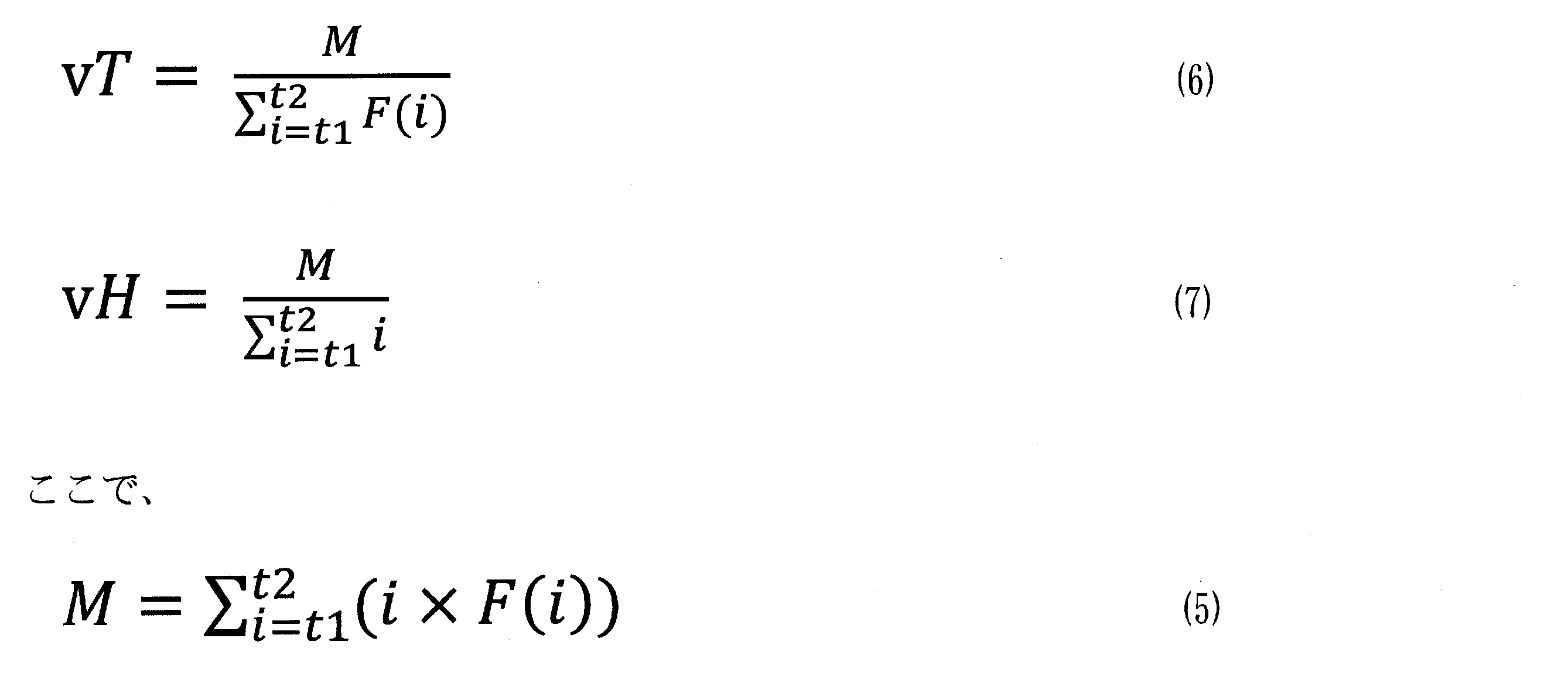
〔2〕記載の分析方法。
〔4〕前記重心点に関係する情報が、前記vT、前記vH、ピーク幅vB、重心ピーク幅vW、B扁平率vAB、B時間率vTB、W扁平率vAW、W時間率vTW、平均時間vTa、平均高さvHa、vTm、vABa及びvAWaからなる群より選択される1つ以上のパラメータを含み、
該ピーク幅vBが、前記t1からt2までのF(t)≧xとなる時間長であり、
該重心ピーク幅vWが、前記t1からt2までのF(t)≧vHとなる時間長であり、
該vABが、該vHと該vBとの比を表し、
該vTBが、該vTと該vBとの比を表し、
該vAWが、該vHと該vWとの比を表し、
該vTWが、該vTと該vWとの比を表し、
該vTa、該vHa、及び該vTmは、F(t)、t1及びt2が前記と同じ定義であり、F(t1)からF(t2)までのデータ点数をnとするとき、それぞれ下記式で表され、

該vABaが、該vHaと該vBとの比を表し、
該vAWaが、該vHaと該vWとの比を表す、
〔3〕記載の分析方法。
〔5〕前記微分曲線の重心点が、重心時間pT及び重心高さpHで規定される座標(pT, pH)で表される前記2次微分曲線のプラスピークの重心点であり、該pT及び該pHは、該2次微分曲線をF'(t)(tは時間)、F'(t)が所定値xである時間をt1、t2(t1<t2)とするとき、下記式で表される、
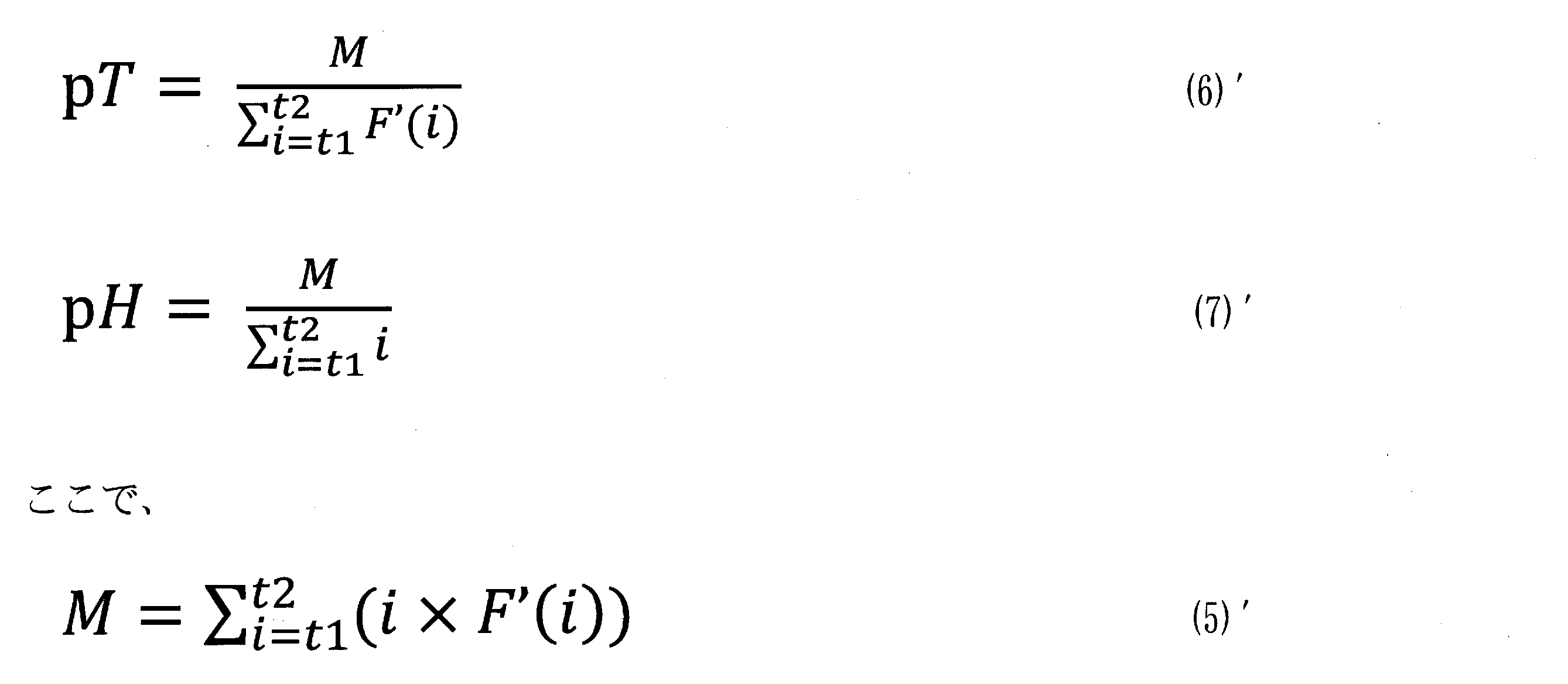
〔2〕記載の分析方法。
〔6〕前記重心点に関係する情報が、前記pT、前記pH、ピーク幅pB、重心ピーク幅pW、B扁平率pAB、B時間率pTB、W扁平率pAW、及びW時間率pTWからなる群より選択される1つ以上のパラメータを含み、
該ピーク幅pBが、前記t1からt2までのF'(t)≧xとなる時間長であり、
該重心ピーク幅pWが、前記t1からt2までのF'(t)≧pHとなる時間長であり、
該pABが、該pHと該pBとの比を表し、
該pTBが、該pTと該pBとの比を表し、
該pAWが、該pHと該pWとの比を表し、
該pTWが、該pTと該pWとの比を表す、
〔5〕記載の分析方法。
〔7〕前記微分曲線の重心点が、重心時間mT及び重心高さmHで規定される座標(mT, mH)で表される前記2次微分曲線のマイナスピークの重心点であり、該mT及び該mHは、該2次微分曲線をF'(t)(tは時間)、F'(t)が所定値xである時間をt1、t2(t1<t2)とするとき、下記式で表される、

〔2〕記載の分析方法。
〔8〕前記重心点に関係する情報が、前記mT、前記mH、ピーク幅mB、重心ピーク幅mW、B扁平率mAB、B時間率mTB、W扁平率mAW、及びW時間率mTWからなる群より選択される1つ以上のパラメータを含み、
該ピーク幅mBが、前記t1からt2までのF'(t)≦xとなる時間長であり、
該重心ピーク幅mWが、前記t1からt2までのF'(t)≦mHとなる時間長であり、
該mABが、該mHと該mBとの比を表し、
該mTBが、該mTと該mBとの比を表し、
該mAWが、該mHと該mWとの比を表し、
該mTWが、該mTと該mWとの比を表す、
〔7〕記載の分析方法。
〔9〕前記所定値xが、前記1次微分曲線F(t)の最大値の0.5~99%である値である、〔3〕~〔8〕のいずれか1項記載の分析方法。
〔10〕前記凝固特性が凝固因子濃度であり、該凝固因子が、凝固第V因子、凝固第VIII因子、凝固第IX因子、凝固第X因子、凝固第XI因子、及び凝固第XII因子からなる群より選択される少なくとも1種である、〔4〕、〔6〕又は〔8〕記載の分析方法。
〔11〕前記(4)が、分析対象成分の濃度と前記扁平率との関係と、得られた前記扁平率とに基づいて、分析対象成分を定性すること及び分析対象成分の濃度を定量することを含む、〔4〕、〔6〕又は〔8〕記載の分析方法。
〔12〕前記(4)が、前記重心時間と前記ピーク幅との比(時間率)を用いた解析を含む、〔4〕、〔6〕又は〔8〕記載の分析方法。
〔13〕前記(4)が、前記時間率に基づいて、凝固時間延長の要因が凝固第VIII因子であるか否かを判定することを含む、〔12〕記載の分析方法。
〔14〕前記(4)が、分析対象成分の濃度と前記時間率との関係と、得られた前記時間率とに基づいて、分析対象成分を定性すること及び分析対象成分の濃度を定量することを含む、〔12〕又は〔13〕記載の分析方法。
〔15〕前記凝固反応曲線のデータは、活性化部分トロンボプラスチン時間の測定によって得られたデータである、〔1〕~〔14〕のいずれか1項記載の分析方法。
〔16〕前記(2)が、取得した前記凝固反応曲線のデータの最大値に基づいて補正処理を行って補正処理済み凝固反応曲線のデータを算出することを更に含み、かつ
該(2)において、前記微分曲線のデータの算出には該補正処理済み凝固反応曲線のデータを用いる、
〔1〕~〔15〕のいずれか1項記載の分析方法。
〔17〕前記(1)が、
被検血漿と正常血漿とを混合した混合血漿を調製することと、
該混合血漿の加温処理なしでの凝固時間測定を行うことと、
該混合血漿の加温処理後の凝固時間測定を行うことと、
を含み、
前記(3)が、
該混合血漿の加温処理なしでの凝固時間測定データに基づいて凝固反応状態と関係する第1のパラメータを算出することと、
該混合血漿の加温処理後の凝固時間測定データに基づいて凝固反応状態と関係する第2のパラメータを算出することと、
を含み、
前記(4)が、
該第1のパラメータと該第2のパラメータとの比又は差に基づいて、凝固時間の延長の要因を鑑別することと
を含む、
〔1〕~〔16〕のいずれか1項記載の分析方法。
〔18〕前記凝固時間測定は、プロトロンビン時間測定、活性化部分トロンボプラスチン時間測定、希釈プロトロンビン時間測定、希釈部分トロンボプラスチン時間測定、カオリン凝固時間測定、及び希釈ラッセル蛇毒時間測定のうち、少なくとも何れか1つである、〔17〕記載の分析方法。
〔19〕前記鑑別は、凝固時間の延長の要因が凝固因子インヒビターの影響であるかループスアンチコアグラントの影響であるかを判定することを含む、〔17〕又は〔18〕記載の分析方法。
〔20〕前記混合血漿の加温時間は2分以上30分以下である、〔17〕~〔19〕のいずれか1項記載の分析方法。
〔21〕前記第1のパラメータ及び前記第2のパラメータが、前記1次微分曲線の最大値、重心高さvH、重心時間vT、ピーク幅vB、重心ピーク幅vW、B扁平率vAB、B時間率vTB、W扁平率vAW、W時間率vTW、平均時間vTa、平均高さvHa、vTm、ABa及びvAWaからなる群より選択される少なくとも1つを含む、請求項17~20のいずれか1項記載の分析方法。
〔17〕~〔20〕のいずれか1項記載の分析方法。
〔22〕前記鑑別は、前記第1のパラメータと前記第2のパラメータとの比が1を含む所定の範囲内に収まらない場合に、凝固時間の延長の要因が凝固因子インヒビターの影響にあると判定することを含む、〔17〕~〔21〕のいずれか1項記載の分析方法。
〔23〕前記鑑別は、前記第1のパラメータと前記第2のパラメータとの比が1を含む所定の範囲内に収まる場合に、凝固時間の延長の要因はループスアンチコアグラントの影響にあると判定することを含む、〔17〕~〔21〕のいずれか1項記載の分析方法。
〔24〕前記鑑別は、前記第1のパラメータと前記第2のパラメータとの差が0を含む所定の範囲内に収まらない場合に、凝固時間の延長の要因が凝固因子インヒビターの影響にあると判定することを含む、〔17〕~〔21〕のいずれか1項記載の分析方法。
〔25〕前記鑑別は、前記第1のパラメータと前記第2のパラメータとの差が0を含む所定の範囲内に収まる場合に、凝固時間の延長の要因はループスアンチコアグラントの影響にあると判定することを含む、〔17〕~〔21〕のいずれか1項記載の分析方法。
〔26〕前記被検血漿と前記正常血漿との混合比は1対1である、〔17〕~〔25〕のいずれか1項記載の分析方法。
〔27〕前記混合血漿の加温処理温度は35℃以上39℃以下である、〔17〕~〔26〕のいずれか1項記載の分析方法。
〔28〕〔1〕~〔27〕のいずれか1項記載の分析方法を実行するための分析装置。
1.1.分析方法の概要
本実施形態に係る分析方法の概要を図1に示すフローチャートを参照して説明する。初めに、検体に関して、検査に用いられる試料が調製される(ステップS101)。調製された試料を対象として、凝固時間の測定が実行される(ステップS102)。凝固時間の測定の例として、APTT、PTなどの測定が挙げられる。凝固時間の測定で得られたデータに対する所定の解析が行われる(ステップS103)。解析結果に基づいて、検体について血液凝固機能に関する評価が行われる(ステップS104)。
ステップS101として行われる試料の調製と、ステップS102として行われる凝固時間の測定について説明する。ここでは、凝固時間の測定として、特にAPTTの測定を例に挙げて説明する。
1.3.1.データ解析の概略
ステップS103として行われるデータ解析について説明する。図2は、データ解析の概略を示すフローチャートである。
P(t)=[(D(t)-Dmin)/Drange]×100 (1)
ステップS204で行われる凝固反応曲線(0次曲線)の微分曲線の算出の一例について説明する。凝固反応曲線A(n)から1次曲線B(n)を得るための微分処理としては、下記式(2)を用いた差分法が用いられ得る。
B(n)=A(n)-A(n-1) (2)


本実施形態では、上記の0次曲線、1次曲線、及び2次曲線に基づいて、種々の評価パラメータが算出される。それらパラメータについて説明する。
本実施形態の評価パラメータの1つである凝固時間について、図9に示すベースライン調整後の凝固反応曲線を参照して説明する。ベースライン調整後の凝固反応曲線における散乱光量の変化量が所定条件を満たした時点を凝固終了判定点Teとする。例えば、単位時間当たりの散乱光量の変化量が所定値以下となった時点を凝固終了判定点Teとする。この凝固終了判定点Teの散乱光量を100%としたときに、散乱光量がc%に相当する反応経過時間を、凝固時間Tcとする。例えば、散乱光量が50%に相当する反応経過時間を、凝固時間T50とする。このように凝固時間Tcを定義することで、APTT測定中に、ベースライン調整後の凝固反応曲線が所定条件を満たした凝固終了判定点Te(=T100)が検出されたときに、直ちに凝固時間Tcが決定され得る。なお、凝固時間Tcの決定方法については本方法に限らない。他の方法により凝固時間が定義されてもよい。例えば、凝固速度が最大になる時間を凝固時間としてもよいし、図6に示したような補正後の散乱光量が50%となる反応経過時間T50を凝固時間Tcとしてもよい。
演算対象域値について、図10Aを参照して説明する。図10Aは、補正1次曲線の一例を示す。補正1次微分(凝固進行率)の最大値Vmaxも評価パラメータになり得る。ここでは、補正1次曲線を例に挙げたが、未補正1次曲線でも同様である。凝固速度の最大値も評価パラメータになり得る。
1次曲線における重心点について、図10Aを参照して説明する。図10Aでは、補正1次曲線がF(t)で示される。このときに、F(t)について、演算対象域値Sがx%以上の値を演算対象データとした「重み付き平均値」に相当する位置を重心点(vTx, vHx)とする。

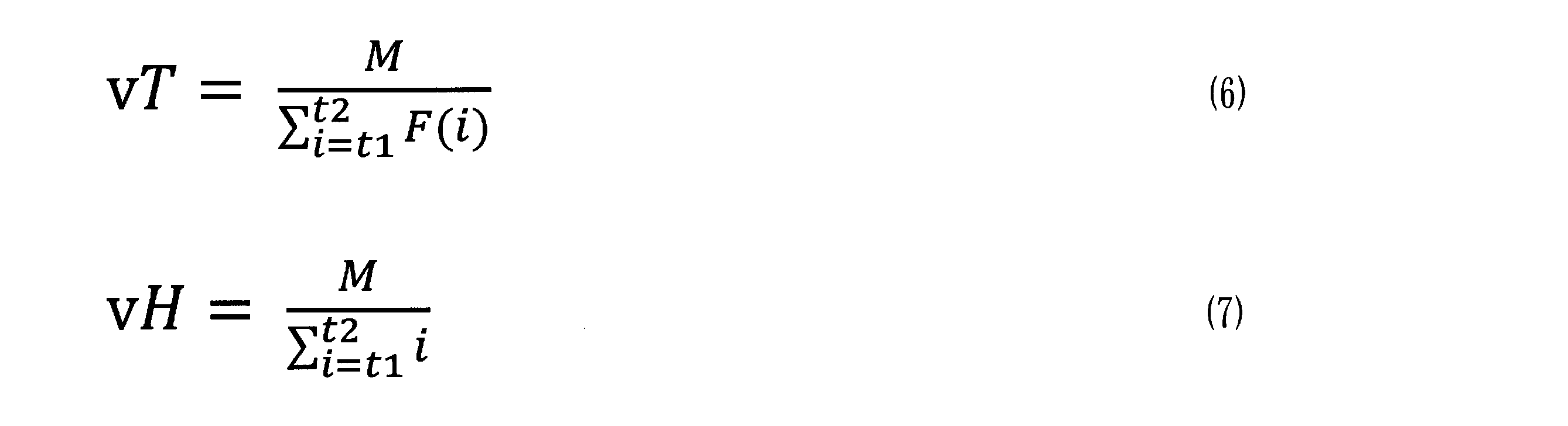
反応時間が重心時間vTより短い領域において1次微分値が演算対象域値S以上となる最少の反応時間から、反応時間が重心時間vTより長い領域において1次微分値が演算対象域値S以上となる最大の反応時間までの時間のうち、F(t)≧Sとなる時間長(F(t)≧Sとなるデータ点数から1を引いたものに測光時間間隔を乗じて得られた値)を、1次曲線のピーク幅vBとする。図10Aに示す例では、時刻vTsから時刻vTeまでがピーク幅vBとなる。同様に、2次曲線のプラスピークにおける2次微分値が演算対象域値S以上となる反応時間の最小値及び最大値はそれぞれpTs、pTeであり、pTsからpTeまでの時間のうち、F’(t)≧Sとなる時間長(F’(t)≧Sとなるデータ点数から1を引いたものに測光時間間隔を乗じて得られた値)を2次曲線のプラスピークのピーク幅pBとする。同様に、2次曲線のマイナスピークにおける2次微分値が演算対象域値S以下となる反応時間の最小値及び最大値はそれぞれmTs、mTeであり、mTsからmTeまでの時間のうち、F’(t)≦Sとなる時間長(F’(t)≦Sとなるデータ点数から1を引いたものに測光時間間隔を乗じて得られた値)を2次曲線のマイナスピークのピーク幅mBとする。
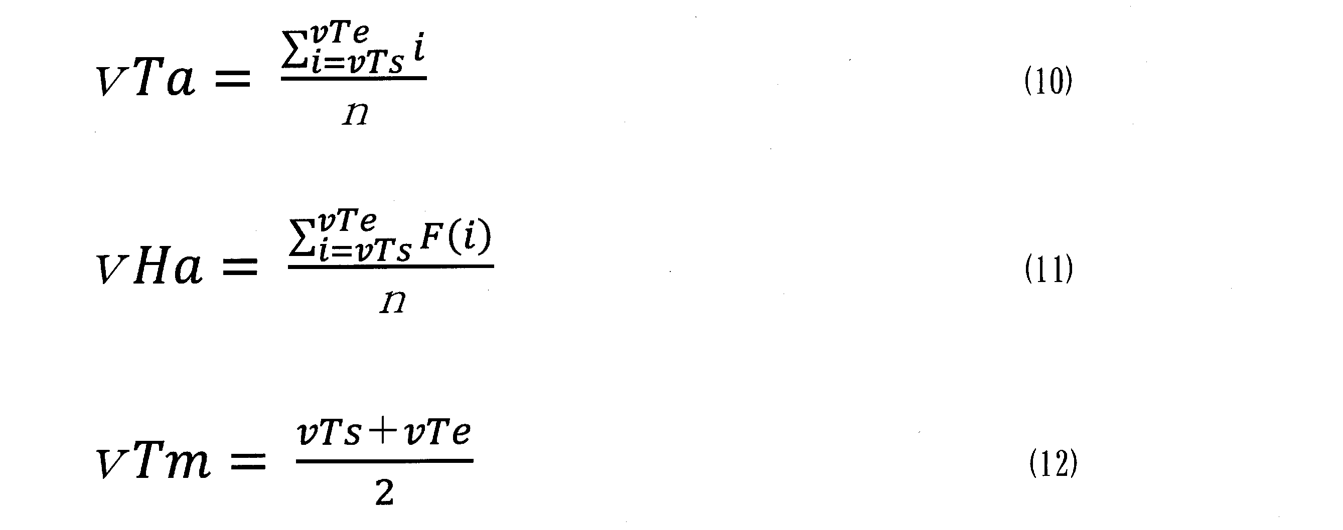
vAB=vH/vB (8a)
vAW=vH/vW (8b)
vABa=vHa/vB (8c)
vAWa=vHa/vW (8d)
vTB=vT/vB (9a)
vTW=vT/vW (9b)
本発明で用いられる重心点に関係するパラメータのさらなる例としては、1次曲線又は2次曲線の演算対象域における曲線下面積(AUC)が挙げられる。2次曲線はプラス側ピークとマイナス側ピークを有するため、2次曲線の最大ピーク高さを100%とした演算対象域における曲線下面積(AUC)は、プラス側ピークについての演算対象域におけるAUC(pAUC)とマイナス側ピークの演算対象域におけるAUC(mAUC)があり得る。本明細書においては、異なる演算対象域に由来するAUCを識別するため、それが由来する演算対象域値Sに従って、AUCxと称することがある。例えば、Sが5%である演算対象域のvAUC、pAUC、及びmAUCは、それぞれvAUC5%、pAUC5%、及びmAUC5%である。さらに、上述の重心点に関係するパラメータ以外のさらなるパラメータが、本発明で用いられるパラメータに含まれ得る。該パラメータの例としては、上述の凝固時間Tc、最大1次微分値Vmax、最大2次微分値Amax、最小2次微分値Amin、及びそれらに到達する時間を表すVmaxT、AmaxT、AminTなどが挙げられる。これらのパラメータも、評価パラメータとして使用され得る。
ステップS104で行われる評価の一例について説明する。
・第VIII因子の濃度に対して、T50、vH、vT、vTe、vTr、vTa、vHa、vTm、vB、vW、vAB、vTB、vAW、pH、pAB、pAW、pAUC、VmaxT、Amax、AmaxT、mAUC、又はそれらの2種以上の組み合わせ。このときの演算対象域Sは、Vmaxが100%のとき、好ましくは0.5~99%、より好ましくは1~95%、さらに好ましくは5~80%、さらに好ましくは30~80%、さらに好ましくは30~70%又は50~80%である。
・第IX因子の濃度に対して、T50、vT、vTs、vTa、vTm、pT、又はそれらの2種以上の組み合わせ。このときの演算対象域Sは、Vmaxが100%のとき、0.5~99%、より好ましくは10~95%、さらに好ましくは10~80%である。
1次曲線のピーク形状は、正常検体では単峰性になることが多いが、試薬の種類や検体に含まれる凝固機能関与成分の影響の差異などによって二峰性になったり、ショルダー状の曲線になったりする場合がある。例えば、特許文献1乃至3に開示されている技術のように、凝固速度の最大値を評価パラメータとして用いる場合に、実際は凝固速度曲線が単峰性の形状とならないような場合であっても強力なスムージング処理によって単峰性となる凝固速度曲線を得て、凝固速度の最大値を特定することがある。しかしながら、このようなスムージング処理によって、測定データに含まれている有用な情報が失われているおそれがある。血液凝固反応では様々な因子が複雑に作用している。種々の形状の1次曲線及び2次曲線は、そのような様々な因子に関する情報を含んでいる可能性がある。本実施形態に係る分析方法は、重心点に関係する評価パラメータを用いることで、必要な情報を失う程の過度のスムージング処理などを行う必要がない。したがって、本実施形態に係る分析方法によれば、様々な因子の状態を詳細に反映した分析結果を得ることができる。
本発明のさらなる一態様は、
被検血漿と正常血漿とを混合した混合血漿を調製することと、
前記混合血漿の加温処理なしでの凝固時間測定を行うことと、
前記混合血漿の加温処理後の凝固時間測定を行うことと、
前記混合血漿の加温処理なしでの凝固時間測定データに基づいて凝固反応状態と関係する第1のパラメータを算出することと、
前記混合血漿の加温処理後の凝固時間測定データに基づいて凝固反応状態と関係する第2のパラメータを算出することと、
前記第1のパラメータと前記第2のパラメータとの比又は差に基づいて、凝固時間の延長の要因を鑑別することと、
を含む、血液検体の凝固特性の分析方法に関する。
本実施形態に係る分析方法の概要を図1に示すフローチャートを参照して説明する。
ステップS101として行われる試料の調製と、ステップS102として行われるAPTT測定について説明する。検査対象となる検体は、上記1.2.で述べたとおりである。試料の調製では、被検血漿と、別途に準備した正常血漿とが所定容量比率で混合される。被検血漿と正常血漿との混合比は、合計を10容量とした容量比で、被検血漿:正常血漿=1:9~9:1の範囲であればよく、好ましくは4:6~6:4の範囲、より好ましくは5:5である。例えば1:1、1:4、4:1である。
上記1.3.で述べた手順に従って、分析対象である加温処理なし及び加温処理後の混合血漿のについてのデータが取得される。上記1.3.1.及び1.3.2.で述べた手順に従って、加温処理なし及び加温処理後のそれぞれの混合血漿についての凝固反応曲線に対して、平滑化処理、ゼロ点調整を行うことができ、又は補正処理済み凝固反応曲線を得ることができ、さらに得られた補正処理済み凝固反応曲線及び補正処理なし凝固反応曲線(0次曲線)から、1次曲線、又は2次曲線を取得することができる。得られた曲線から、種々の評価パラメータが算出される。取得される評価パラメータの詳細は、上記1.3.3.で述べたとおりである。
ステップS104で行われる評価の一例について説明する。本実施形態では、例えばLAといった抗リン脂質抗体が延長要因の場合、加温処理有無によるAPTTの変化はあまり認められないのに対して、インヒビターが要因の場合、加温処理後にAPTTが延長することが高感度に検出される。
上述のデータ解析及び評価は、コンピュータを用いて自動的に行われ得る。また、試料の調製及び凝固時間の測定も含めて、上述の一連の分析は、自動分析装置によって、自動的に行われ得る。このような分析を行う自動分析装置について、説明する。
図13は、本実施形態に係る自動分析装置1の構成例の概略を示すブロック図である。自動分析装置1は、制御ユニット10と、測定ユニット30と、タッチスクリーン90とを備える。
3.2.1.動作の概略
本実施形態に係る自動分析装置1の動作について説明する。図14は、制御ユニット10の動作の概略を示す図である。
図15は、測定ユニット30が行う測定に関する動作の概略を示すフローチャートである。
ステップS305において行われる分析処理の一例について、図16に示すフローチャートを参照して説明する。ここに示す分析処理は、分析対象についての、上述した例えばAPTTといった凝固時間の測定データを解析して、種々の評価パラメータを算出し、得られた評価パラメータに基づいて、血液凝固の異常の有無など血液凝固に関する特性を解析する処理である。ここで、分析対象は、上記1.2.で述べたような被検血漿であってもよく、又は上記2.2.で述べたような混合血漿(加温血漿及び非加温血漿)であってもよい。

4.1.方法
4.1.1.血液検体の凝固反応の測定方法
血液凝固因子に起因して異常のある被験者に由来する血液検体と正常な血液検体(正常血漿)を特定の割合で混合した複数の混合試料について、本実施形態に係る解析を行った。すなわち、複数の混合試料の各々と、凝固時間測定試薬とを混和した測定対象試料を用意した。測定対象試料の凝固反応データとして、散乱光量の測光データを取得した。取得した測光データについて本実施形態に係る解析を行った。
上述のようにして取得した凝固反応の経時的な測光データを、凝固反応曲線とした。この凝固反応曲線に関して、解析を行った。まず、凝固反応曲線に対して、ベースライン調整を行った。すなわち、凝固反応曲線に対してノイズ除去を含む平滑化処理を行い、測定開始時点の散乱光量が0となるように調整した。続いて、凝固反応曲線(未補正0次曲線)の最大高さが100となるように補正し、補正処理済み凝固反応曲線(補正0次曲線)を得た。補正0次曲線を1次微分して、補正1次曲線を得た。補正1次曲線の算出には、上述の式(4)による区間内平均傾きを用いた。
4.2.1. 0次曲線及び1次曲線
図17Aに、得られた凝固反応曲線(未補正0次曲線)の例を示す。実線は、正常血漿の未補正0次曲線を示し、破線は、第VIII因子濃度0.1%以下の未補正0次曲線を示し、一点鎖線は、第IX因子濃度0.1%以下の未補正0次曲線を示す。図17Bは、図17Aに示した各検体の未補正0次曲線について、それぞれ散乱光量の最大値が100となるように補正した、補正0次曲線を示す。
図19Aは、第VIII因子濃度の対数に対する凝固時間の関係を示す。なお、濃度0.1%以下に関して対数変換をするときには、濃度0.1%として計算した。他の図においても同様である。この図において、三角印(△)は1次微分値が最大値となる時間(VmaxT)を示し、丸印(○)は重心時間vTを示す。重心時間vTを求めるにあたって、演算対象域値Sは10%に設定した。図19Bは、第IX因子濃度の対数に対する凝固時間の関係を示す。この図において、三角印(△)は1次微分値が最大値となる時間(VmaxT)を示し、丸印(○)は重心時間vTを示す。重心時間vTを求めるにあたって、演算対象域値Sは10%に設定した。
図21Aは、正常血漿の補正1次曲線を示す。図21Bは、第VIII因子欠乏血漿(Factor FIII Deficient Plasma)の補正1次曲線を示す。図21Cは、第IX因子欠乏血漿(Factor IX Deficient Plasma)の補正1次曲線を示す。各図において、黒丸は、下から順に、演算対象域値Sがそれぞれ10%、20%、30%、40%、50%、60%、70%、80%、90%に設定されたときに得られる重心点を示す。
図24Aは、上記式(2)を用いて算出した、第IX因子欠乏血漿の補正1次曲線の例を示す。図24Bは、上記式(4)を用いて算出した、第IX因子欠乏血漿の補正1次曲線の例を示す。図24Aと図24Bとを比較して明らかなように、図24Bの上記式(4)に基づく方が、1次微分値がより詳細に把握され得る。例えば図24Bでは時間45秒近辺でのサイドピークの情報が詳細に把握され得る。このように区間内平均傾きによる補正1次曲線を用いることで、上述の解析によってより詳細な情報を得ることができることが明らかになった。
5.1.方法
5.1.1.血液検体の凝固反応の測定方法
被検血漿として、第VIII因子欠乏血漿と正常血漿との混和物を用いた。第VIII因子欠乏血漿には、Factor VIII Deficient Plasma(George King Bio-Medical, Inc.製)を用いた。正常血漿には、VIII因子濃度及びIX因子濃度が100%と看做せる正常プール血漿を用いた。被検血漿として、第VIII因子欠乏血漿(George King Bio-Medical, Inc.製)と正常血漿とを混合し、第VIII因子濃度が50%、25%、10%、5%、2.5%、1%、0.75%、0.5%及び0.25%となるように調製した試料、及び第VIII因子欠乏血漿(第VIII因子濃度が0.1%以下)を用いた。
測光データを基にして補正1次曲線を得る手順は、第1の実施例と同じ手順とした。
5.2.1.補正処理の有効性について
ステップS203の補正処理の効果について検討を行った。第VIII因子濃度が異なる被検血漿に関してAPTT測定を行い、補正0次曲線から得られた補正1次曲線に基づいて、演算対象域値が80%の場合の扁平率vAB80%を算出した。なお、このときの扁平率vABは、値が1以上になるようにするため、定数100を掛けて演算している。また、未補正0次曲線から得られた未補正1次曲線に基づいて、演算対象域値が80%の場合の扁平率RvAB80%を算出した。図25Aは、第VIII因子濃度と補正1次曲線に基づくvAB80%との関係を示す。図25Bは、第VIII因子濃度と未補正1次曲線に基づくRvAB80%との関係を示す。いずれのグラフも横軸は、第VIII因子濃度の対数を示す。図25Bに示す未補正1次曲線より、図25Aに示す補正1次曲線の方が、わずかであるが回帰曲線によく一致した。
被検血漿として、第VIII因子濃度がそれぞれ、50%、25%、10%、5%、2.5%、1%、0.75%、0.5%、0.25%及び0%となる第VIII因子欠乏血漿(以下、それぞれFVIII(50%)、FVIII(25%)、FVIII(10%)、FVIII(5%)、FVIII(2.5%)、FVIII(1%)、FVIII(0.75%)、FVIII(0.5%)、FVIII(0.25%)、FVIII(0%)と表記する)を調製し、APTT測定を行って得られた補正1次曲線を図26に示す。図26に示されるように、補正1次曲線の形状は、以下のようになった。第VIII因子濃度の低下に従って、最大ピーク高さは低下していき、ピーク形状は扁平化していった。また、第VIII因子濃度の低下に従って、二峰性ピークが出現した。
各種の凝固因子欠乏血漿について時間率vTBの解析を行った。演算対象域値をx%に設定したときに得られる評価パラメータとして、重心点の重心時間vTをvTx%と表記し、ピーク幅vBをvBx%と表記し、時間率vTBをvTBx%と表記する。時間率vTBは、vTBx%=(vTx%/vBx%)×100である。
各種凝固因子欠乏血漿について扁平率vABの解析を行った。演算対象域値Sをx%に設定したときに得られる評価パラメータとして、重心点Wの重心高さvHをvHx%と表記し、ピーク幅vBをvBx%と表記し、扁平率vABをvABx%と表記する。扁平率vABは定数100を掛けた、vABx%=vHx%/vBx%である。
6.1.方法
6.1.1.血液検体の凝固反応の測定方法
被検血漿として、第2の実施例と同様に、凝固因子欠乏血漿と正常血漿との混合血漿を調製した。凝固因子欠乏血漿としては、第2の実施例で用いた第V因子欠乏血漿(V)、第VIII因子欠乏血漿(VIII)、第IX因子欠乏血漿(IX)、第X因子欠乏血漿(X)、第XI因子欠乏血漿(XI)及び第XII因子欠乏血漿(XII)を用いた。比較対照用として正常血漿(PNP)を用いた。凝固因子欠乏血漿のみを含む被検血漿(濃度0%)で凝固因子濃度の対数変換をするときには、濃度0.1%として計算した。第1の実施例と同じ手順で各被検血漿のAPTT測定を行った。
第1の実施例と同じ手順で、測光データから未補正0次曲線及び補正0次曲線を得た。得られた未補正0次曲線及び補正0次曲線から、第1の実施例と同様の手順で上述の式(4)による区間内平均傾きを求めることで、未補正1次曲線及び補正1次曲線をそれぞれ算出した。さらに得られた1次曲線に対して同じ計算を繰り返し、未補正2次曲線及び補正2次曲線をそれぞれ算出した。補正0次曲線、補正1次曲線、及び補正2次曲線からパラメータを算出した。
6.2.1.凝固因子に依存した曲線形状の変化
図41Aに、凝固因子欠乏(実施例においては因子濃度を0.1%として取り扱った。)を被検血漿として得られた未補正0次曲線及び未補正1次曲線の例を示す。また図41Bに、同じ被検血漿から得られた補正0次曲線及び補正1次曲線の例を示す。図42Aは、同じ被検血漿から得られた未補正2次曲線の例を示す。図42Aの右図は、図42A左図のy軸方向の縮尺を変えた図である。図42Bは、同じ被検血漿から得られた補正2次曲線の例を示す。図42Bの右図は、図42B左図のy軸方向の縮尺を変えた図である。図41~42から分かるとおり、欠乏する凝固因子の種類によって凝固時間、及び1次曲線及び2次曲線における最大ピークの高さ及び時間が異なっていた。
補正0次~2次曲線から算出したパラメータを表2に示す。演算対象域値xは、ピークの最大値(Vmax、Amax、Amin)を100%としたときの、0%~99%に設定した。なおAPTTとはT50(0次曲線が最大高さの50%に達するまでの時間)を表す。図43A乃至図43Vには、上図に各種凝固因子濃度の対数とパラメータ値の対数との関係を示す。この関係から検量線を作成した。該検量線を基にパラメータ値から演算濃度を算出した。中左図には、X軸が実測濃度、Y軸が演算濃度となるように各種凝固因子の相関関係をプロットした。中右図には、低濃度での相関関係が確認できるように両軸を対数表示でプロットした。中図の下に記載した式は、各凝固因子濃度に対する演算濃度の直線回帰式と相関係数である。
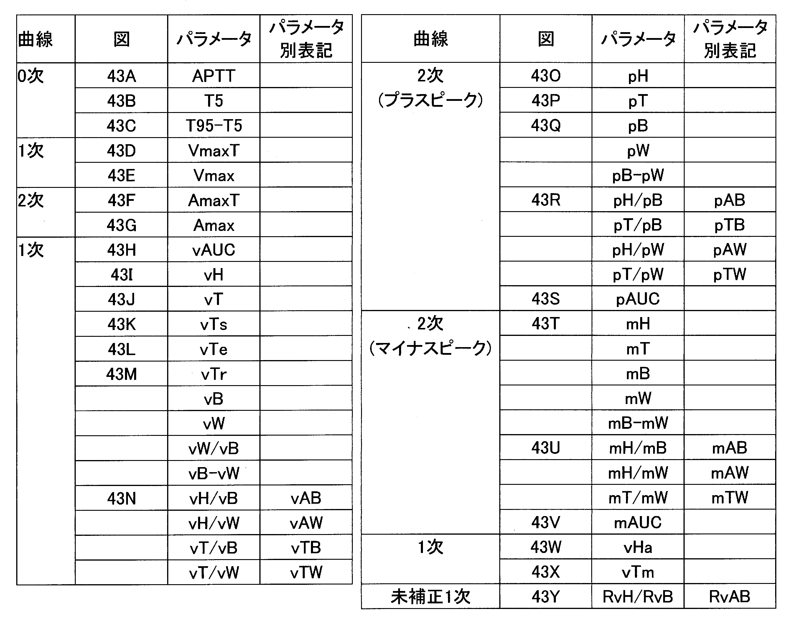
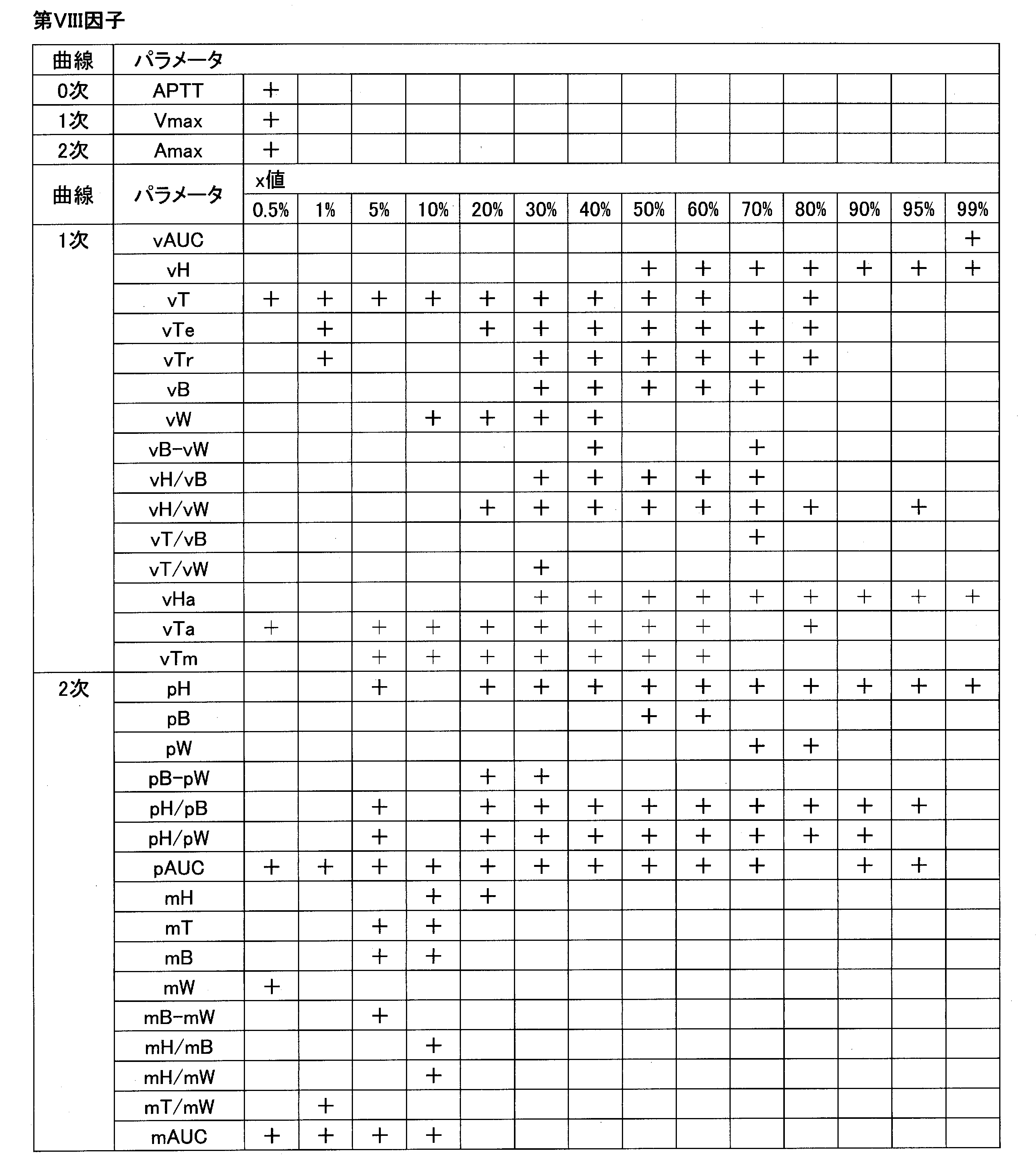
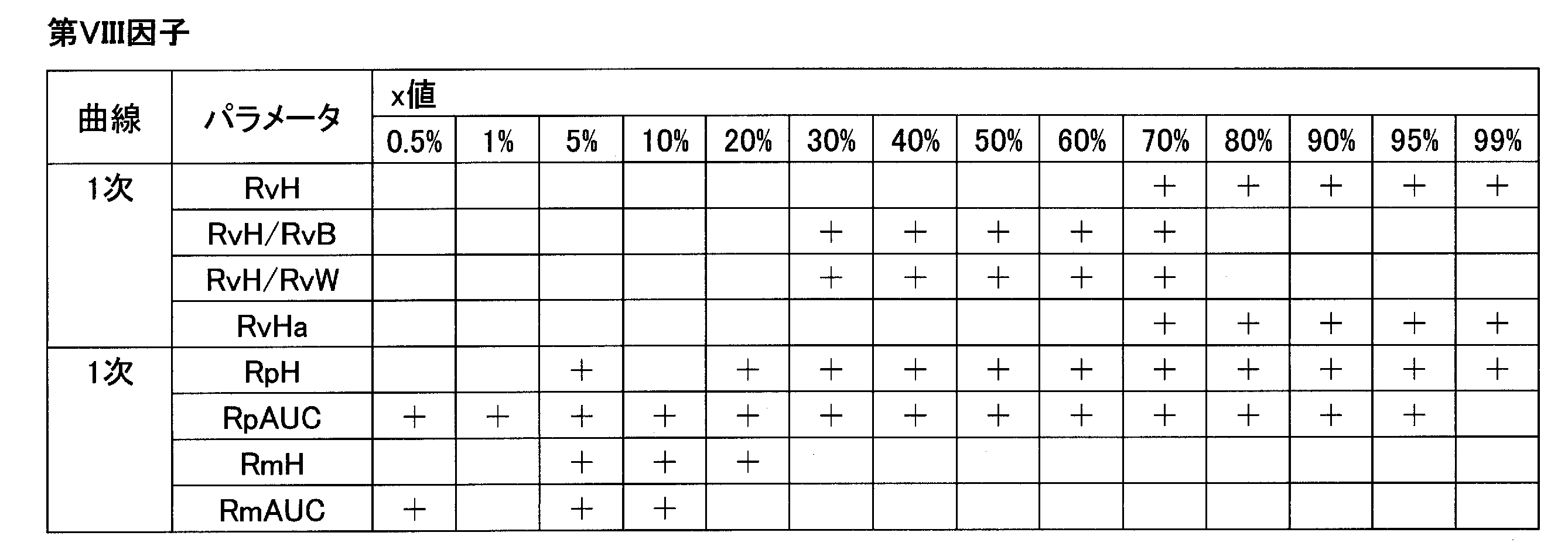
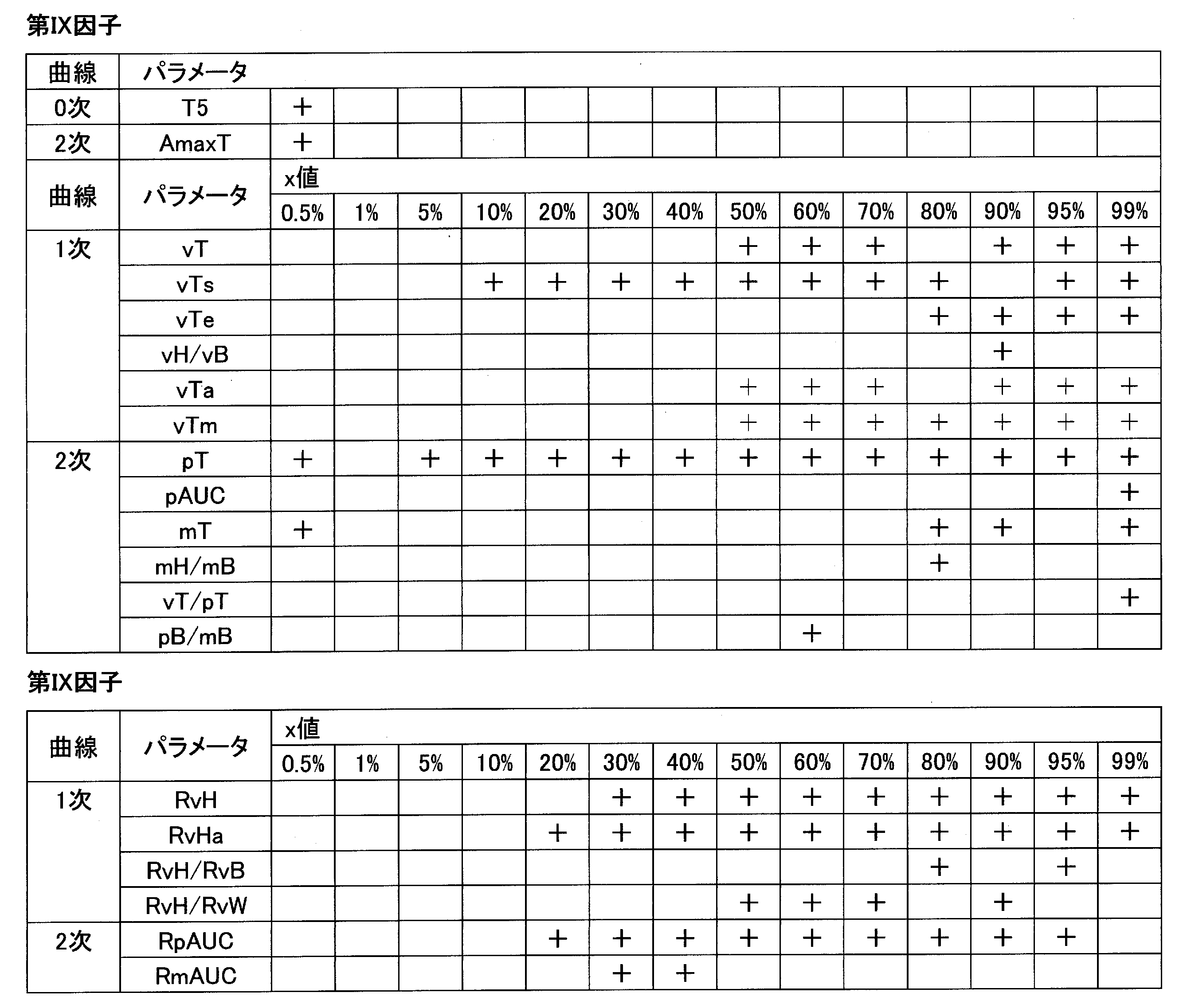


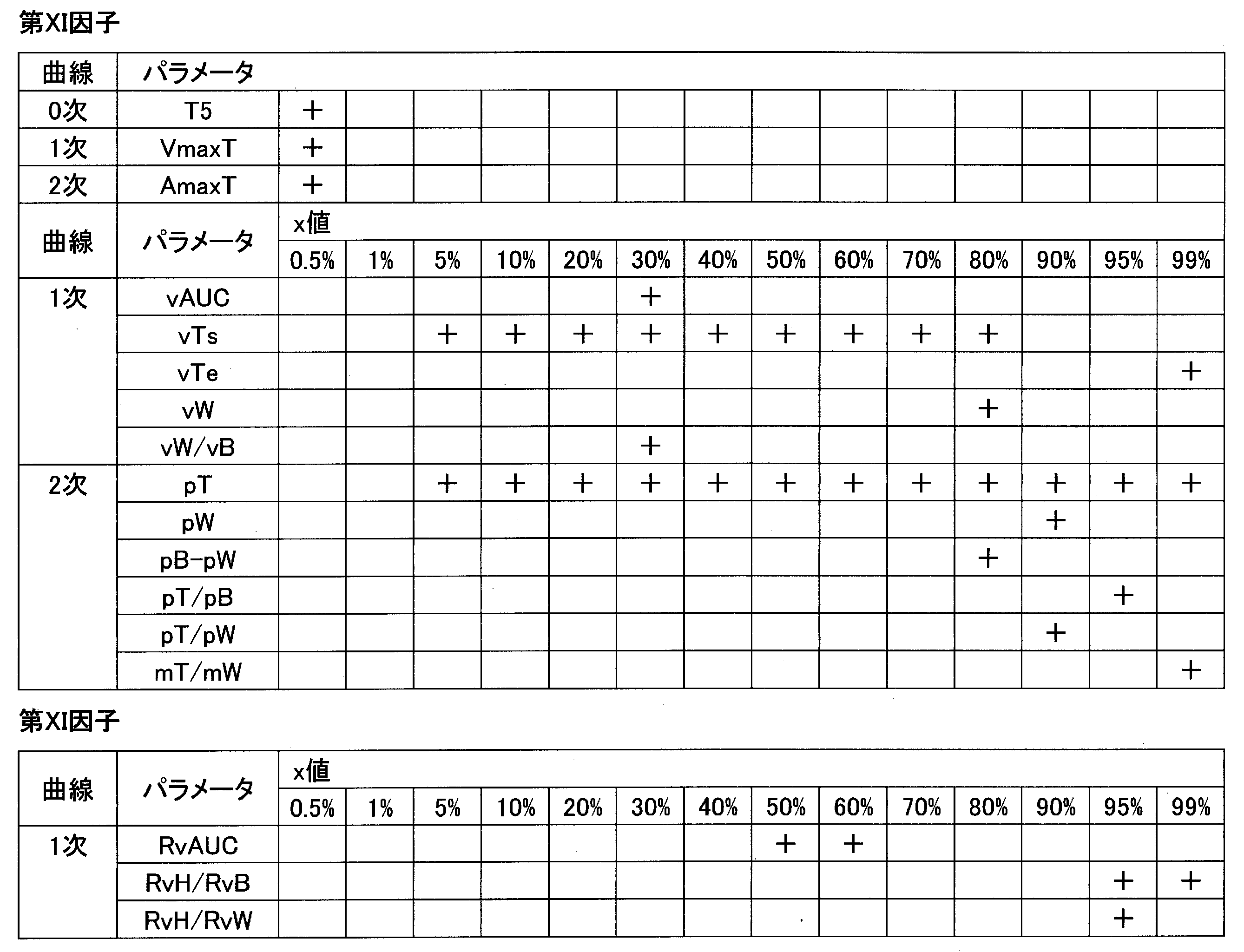


本実施例に示す本発明の実施形態は、被検血漿が凝固異常(APTT延長)を示す場合に、上述した0次曲線~2次曲線に関するパラメータを用いて、APTT延長要因を判定、又はAPTT延長要因が凝固因子インヒビター(抗凝固因子抗体)であった場合には該凝固因子インヒビターの種類の鑑別を実施する方法である。
7.1.1.被検血漿
本実施例で用いた被検血漿を以下に示す。正常血漿(NP)には、健常人より得られたクエン酸加血漿を用いた。LA血漿(LA)には、George King Biomedical, Inc.のPositive Lupus Anticoagulant Plasmaを用いた。第VIII因子欠乏血漿(HA)及び第IX因子欠乏血漿(HB)には、George King BiomedicalのFactor VIII Deficient、Factor IX Deficientを用いた。第VIII因子インヒビター血漿(InL、InM及びInH)には、George King Biomedical, Inc.のFactor VIII Deficient with Inhibitorを用いた。
群No. 検体種 検体数
1 正常血漿(NP) 23
2 LA血漿(LA) 6
3 血友病A(HA) 14
4 血友病B(HB) 12
5 第VIII因子インヒビター低力価血漿(InL)12
6 第VIII因子インヒビター中力価血漿(InM)35
7 第VIII因子インヒビター高力価血漿(InH) 8
なお、インヒビター力価の「低」、「中」、「高」とは、以下を意味する:
中:2~40(BU/mL)(BU/mL:ベセスダ単位)
低:中より低い力価
高:中より高い力価
各被検血漿と正常血漿(NPの混合物)とを1:1の容量比で混合して混合血漿を調製した。
APTT試薬には、コアグピアAPTT-N(積水メディカル株式会社製)を、塩化カルシウム液には、コアグピアAPTT-N 塩化カルシウム液(積水メディカル株式会社製)を用いた。APTT測定には、血液凝固自動分析装置CP3000(積水メディカル株式会社製)を用いた。装置のキュベット(反応容器)に混合血漿50μLを吐出し、以下の手順で通常(非加温)モード又は加温モードで処理した。:
(通常モード)37℃で45秒間の加温
(加温モード)37℃で600~720秒間の加温
その後、キュベットに約37℃に加温したAPTT試薬50μLを添加し、171秒経過後に25mM塩化カルシウム液50μL添加して、凝固反応を開始させた。凝固反応はキュベットを約37℃に維持した状態で行った。凝固反応の検出は、波長660nmのLEDを光源とする光を照射し、0.1秒間隔で90度側方散乱した散乱光量を測光した。測光時間は360秒間とした。同じ混合血漿について、非加温(通常モード)及び加温(加温モード)条件でのAPTT測定をそれぞれ行い、測光データを得た。
非加温血漿及び加温血漿のそれぞれについて得られた測光データに対し、第1の実施例と同様の手順で補正0次~2次曲線を得た。得られた曲線から、表1に示すパラメータを算出した。非加温血漿についてのパラメータをPa、加温血漿についての同じパラメータをPbとし、パラメータ比Pb/Paを求めた。
図44Aに、LA血漿(LA)の加温及び非加温での補正1次曲線を示す。LAでは、加温による曲線形状の変化はほとんどなかった。
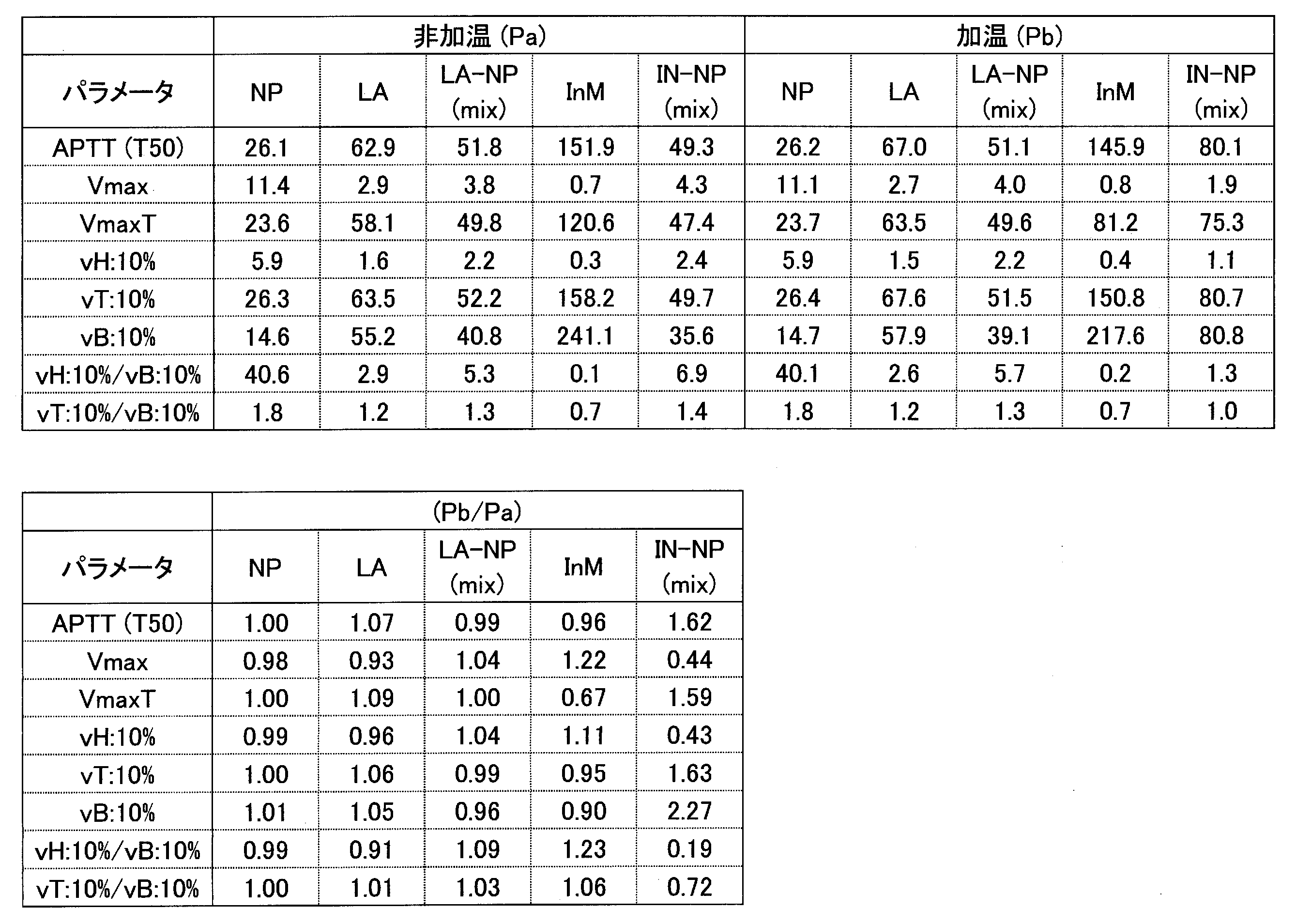
・LAを含む混合血漿は、Pa及びPbともに延長し、Pb/Paは約1である。
・HAとHBを含む混合血漿は、Pa及びPbともに短縮し、Pb/Paは約1である。
・InLを含む混合血漿は、Pa及びPbともに短縮し、Pb/Paは約1である。
・InMを含む混合血漿は、Paで僅かに延長し、PbではPaよりさらに延長し、Pb/Paは1より大になる。
・InHを含む混合血漿は、Paは延長し、PbはPaと同程度かさらに延長し、Pb/Paは約1か又は1より大になる。
(1)PaとPbがともに延長し、かつPb/Paが約1であれば、被検血漿はLA又はInHである。
(2)PaとPbがともに短縮し、かつPb/Paが約1であれば、被検血漿はHAB(HA又はHB)又はInLである。
(3)PaとPbがともに延長し、かつPb/Paが1より大であれば、被検血漿はInM又はInHである。

8.1.方法
8.1.1.血液検体
血液凝固因子に異常のある被験者に由来する血液検体と正常な血液検体(正常血漿)とを用いて、以下の5種類の測定対象試料を用意した。
正常血漿には、CRYOcheck Pooled Normal Plasma(Precision BioLogic Incorporated)を用いた。
LA陽性血漿には、Positive Lupus Anticoagulant Plasma (George King Biomedical,Inc.)を用いた。
第VIII因子インヒビター陽性血漿には、Factor VIII Deficient with Inhibitor (George King Biomedical,Inc.)を用いた。
上で述べた「(2) LA陽性血漿」と「(1) 正常血漿」とを1:1の容量比で混合した混合血漿を調製した。
上で述べた「(3) 第VIII因子インヒビター陽性血漿」と「(1) 正常血漿」とを1:1の容量比で混合した混合血漿を調製した。
上記5種類の試料のそれぞれについて、37℃にて、加温処理なしでのAPTT測定、10分加温処理後のAPTT測定、30分加温処理後のAPTT測定、120分加温処理後のAPTT測定をそれぞれ実施した。
上記5種類の試料のそれぞれについて行われた、加温処理なしでのAPTT測定の結果、10分加温処理後のAPTT測定の結果、30分加温処理後のAPTT測定の結果、120分加温処理後のAPTT測定の結果をそれぞれ示す、経時的な光学的情報、すなわち測光データを取得して凝固反応曲線を得た。
上述した5種類の試料の代表的な補正1次曲線をそれぞれ図47A乃至図47Eに示す。各図の中の4つの曲線M0、M10、M30、M120は、それぞれ、混合血漿の加温処理なし、加温処理10分後、加温処理30分後、加温処理120分後の補正1次曲線を示す。
9.1.方法
第5の実施例では、混合血漿の加温処理時間を10分に設定した場合の実験結果を説明したが、第6の実施例では混合血漿の加温処理時間を2分に設定した場合の実験結果について説明する。第5の実施例と異なる条件は、被検血漿とその数、混合血漿の加温処理時間であり、その他の条件は同じである。
図56は、LA陽性検体のクロスミキシング試験の結果を示す。図において、実線で示したm0は、加温処理なしでのAPTT測定結果を示し、破線で示したm2は、混合血漿の加温処理時間が2分の場合でのAPTT測定結果を示す。図56において、混合血漿加温処理時間が0分(未加温)及び2分で測定結果の差異はほとんどなく、グラフは「上に凸」のパターンを示した。
10.1.方法
第5実施例と同じ手順で、混合血漿(LA陽性血漿について12検体、第VIII因子インヒビター陽性血漿について9検体)を調製し、37℃にて、加温処理なし、及び10分加温処理後にAPTT測定を実施した。取得した測光データから各種評価パラメータを算出し、非加温血漿のパラメータ(Pa)と加温血漿のパラメータ(Pb)との比(Pb/Pa)及び差(Pb-Pa)を求めた。LA陽性血漿と正常血漿との等量混合血漿(LA)と、第VIII因子インヒビター陽性血漿と正常血漿との等量混合血漿(Inhibitor)との間で、該比(Pb/Pa)及び差(Pb-Pa)の分布の平均値の有意差を評価した。各々の分布についてF検定(有意水準1%)により等分散と非等分散を判断し、次いでT検定(両側)でLAの分布とInhibitorの分布の平均値の差のP値を算出した。
図63A~Eに、LA及びInhibitorについての非加温血漿と加温血漿との各種評価パラメータの差(Pb-Pa)及び比(Pb/Pa)の例を示す。図63AはAPTT時間(T50)及びVmax、図63BはvAB40%及びvABa40%、図63CはvH40%及びvHa40%、図63DはvAUC90%及びvW10%/vB10%、図63EはpAUC80%及びmAUC20%についての結果を示す。
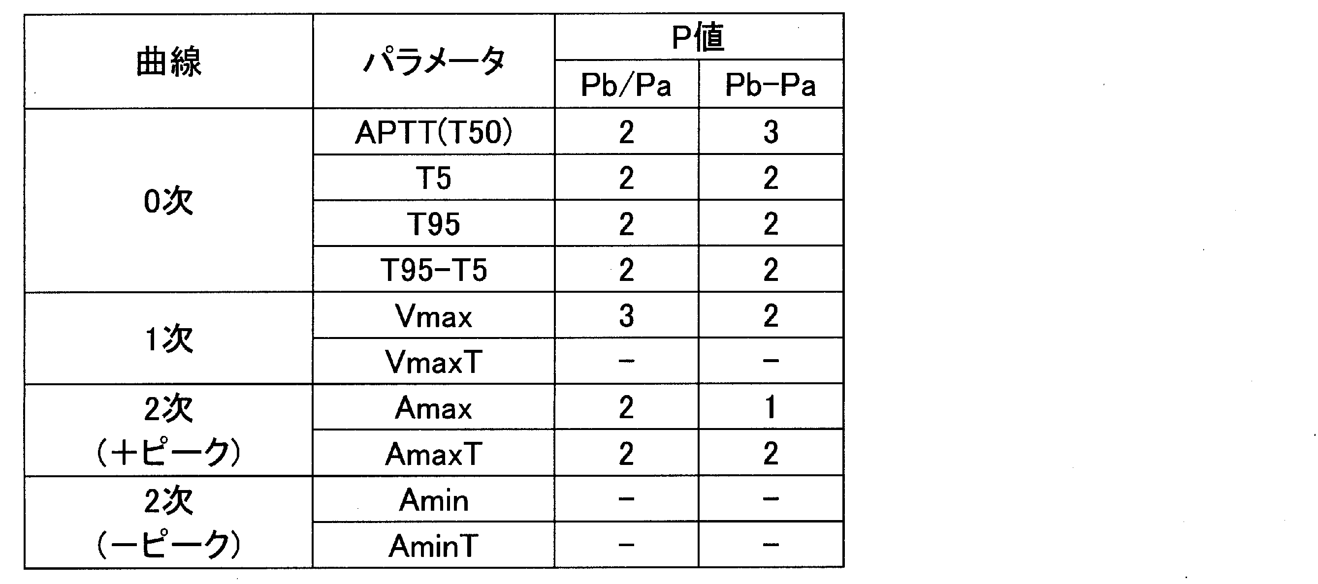

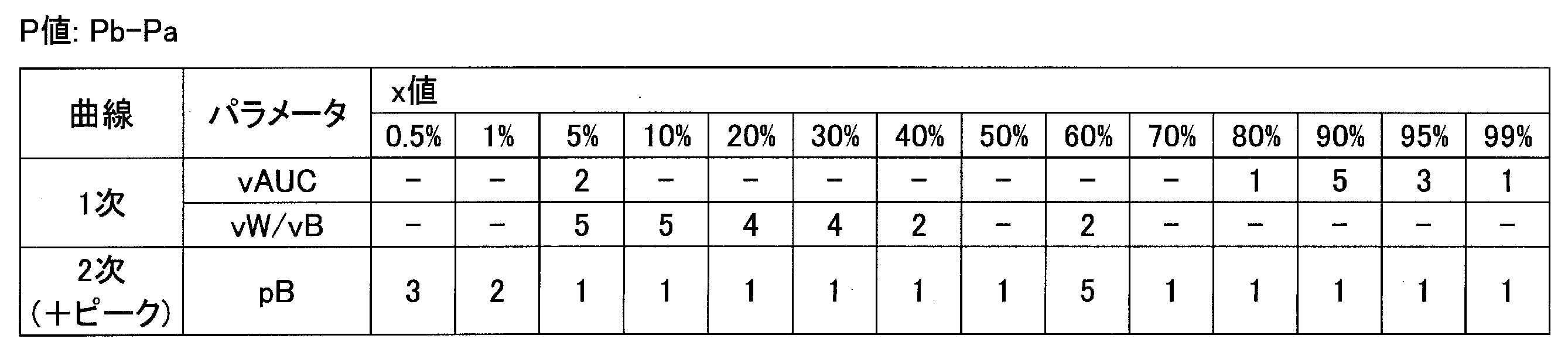

Claims (28)
- 血液検体の凝固特性の分析方法であって、
(1)血液試料と試薬とを含む混合液の、反応時間に対する凝固反応量を示す凝固反応曲線のデータを取得することと、
(2)前記凝固反応曲線に関する微分によって得られる微分曲線のデータを算出することと、
(3)前記微分曲線の重心点に関係する情報を算出することと、
(4)前記重心点に関係する情報を用いて前記血液試料の凝固特性を評価することと、
を含む、方法。 - 前記微分曲線が、前記凝固反応曲線に関する1次微分曲線及び該凝固反応曲線に関する2次微分曲線からなる群より選択される少なくとも1つである、請求項1記載の方法。
- 前記微分曲線の重心点が、重心時間vT及び重心高さvHで規定される座標(vT, vH)で表される前記1次微分曲線の重心点であり、該vT及び該vHは、該1次微分曲線をF(t)(tは時間)、F(t)が所定値xである時間をt1、t2(t1<t2)とするとき、下記式で表される、
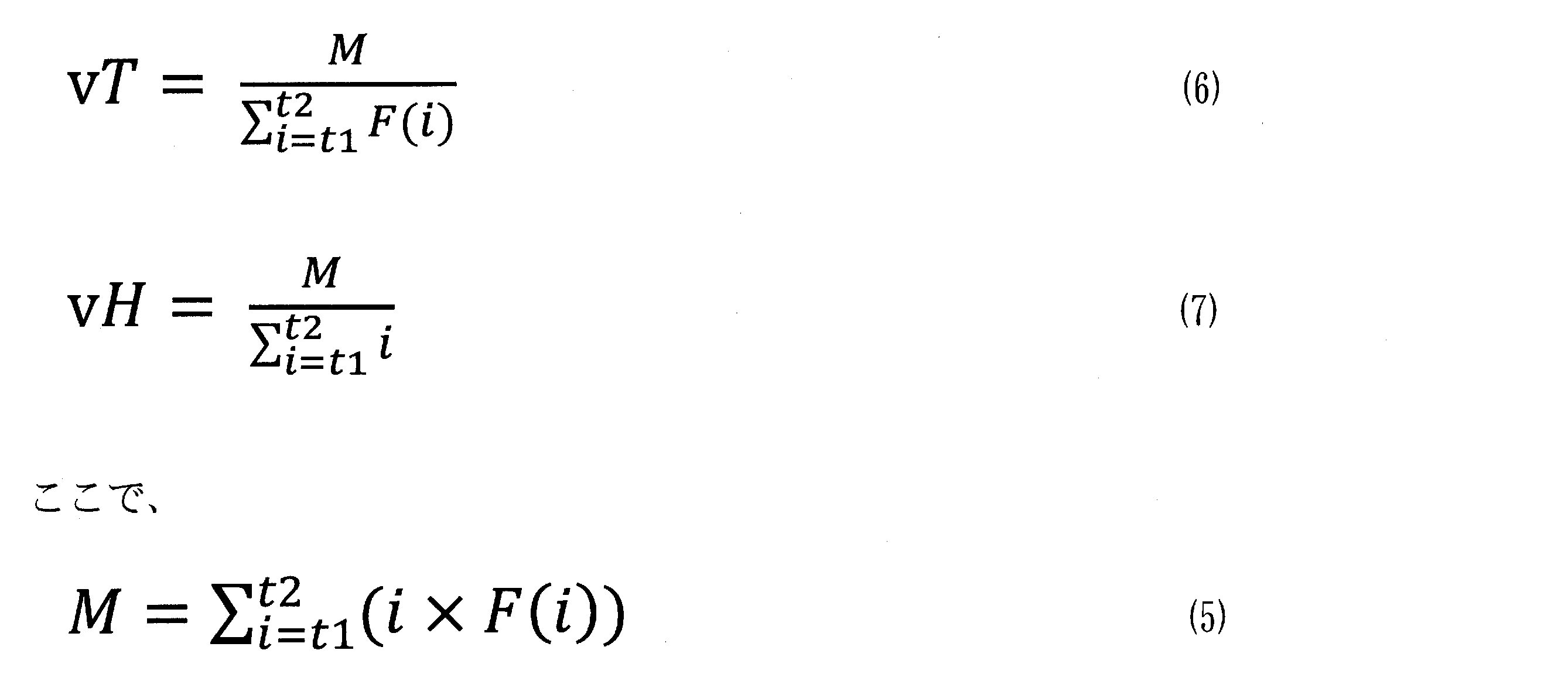
請求項2記載の分析方法。 - 前記重心点に関係する情報が、前記vT、前記vH、ピーク幅vB、重心ピーク幅vW、B扁平率vAB、B時間率vTB、W扁平率vAW、W時間率vTW、平均時間vTa、平均高さvHa、vTm、vABa及びvAWaからなる群より選択される1つ以上のパラメータを含み、
該ピーク幅vBが、前記t1からt2までのF(t)≧xとなる時間長であり、
該重心ピーク幅vWが、前記t1からt2までのF(t)≧vHとなる時間長であり、
該vABが、該vHと該vBとの比を表し、
該vTBが、該vTと該vBとの比を表し、
該vAWが、該vHと該vWとの比を表し、
該vTWが、該vTと該vWとの比を表し、
該vTa、該vHa、及び該vTmは、F(t)、t1及びt2が前記と同じ定義であり、F(t1)からF(t2)までのデータ点数をnとするとき、それぞれ下記式で表され、
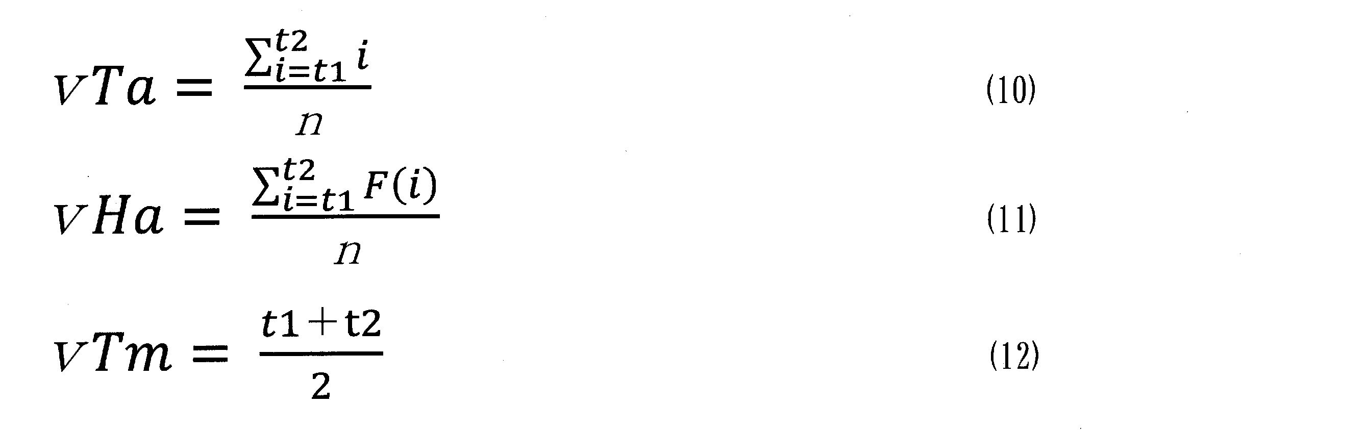
該vABaが、該vHaと該vBとの比を表し、
該vAWaが、該vHaと該vWとの比を表す、
請求項3記載の分析方法。 - 前記微分曲線の重心点が、重心時間pT及び重心高さpHで規定される座標(pT, pH)で表される前記2次微分曲線のプラスピークの重心点であり、該pT及び該pHは、該2次微分曲線をF'(t)(tは時間)、F'(t)が所定値xである時間をt1、t2(t1<t2)とするとき、下記式で表される、

請求項2記載の分析方法。 - 前記重心点に関係する情報が、前記pT、前記pH、ピーク幅pB、重心ピーク幅pW、B扁平率pAB、B時間率pTB、W扁平率pAW、及びW時間率pTWからなる群より選択される1つ以上のパラメータを含み、
該ピーク幅pBが、前記t1からt2までのF'(t)≧xとなる時間長であり、
該重心ピーク幅pWが、前記t1からt2までのF'(t)≧pHとなる時間長であり、
該pABが、該pHと該pBとの比を表し、
該pTBが、該pTと該pBとの比を表し、
該pAWが、該pHと該pWとの比を表し、
該pTWが、該pTと該pWとの比を表す、
請求項5記載の分析方法。 - 前記微分曲線の重心点が、重心時間mT及び重心高さmHで規定される座標(mT, mH)で表される前記2次微分曲線のマイナスピークの重心点であり、該mT及び該mHは、該2次微分曲線をF'(t)(tは時間)、F'(t)が所定値xである時間をt1、t2(t1<t2)とするとき、下記式で表される、
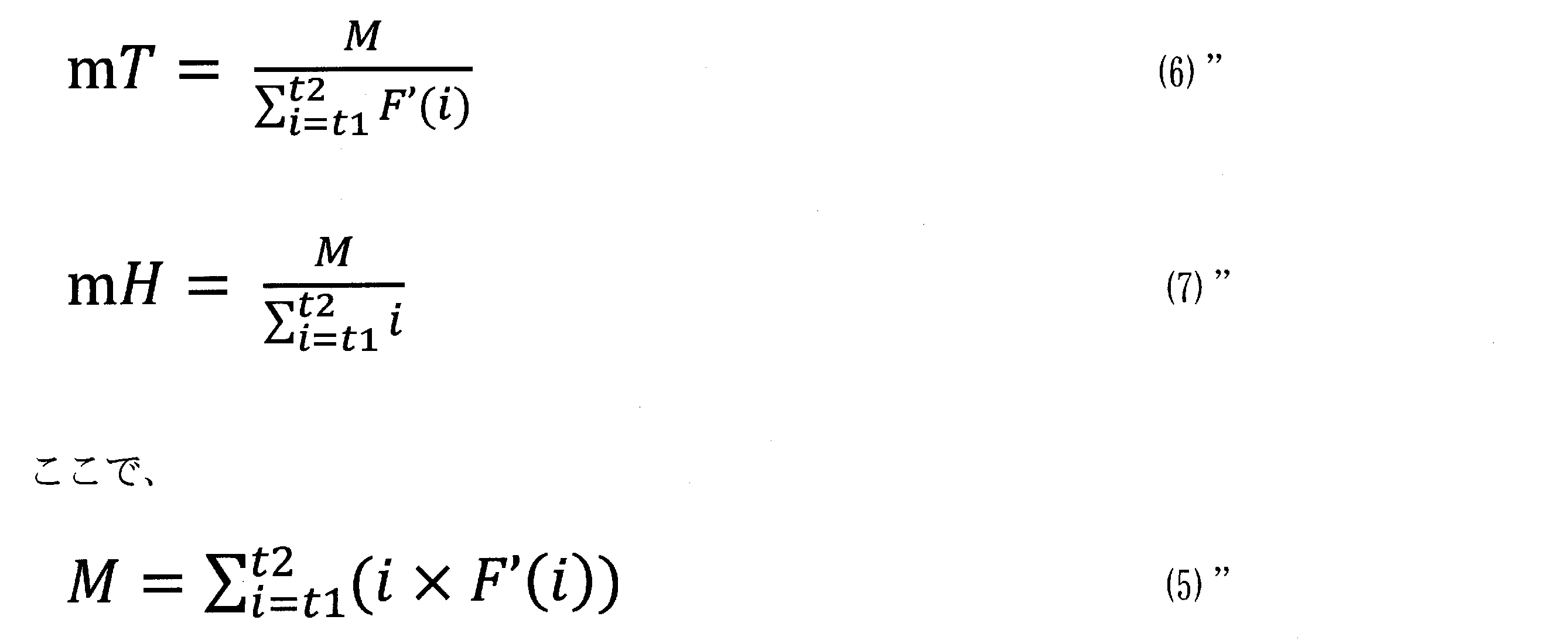
請求項2記載の分析方法。 - 前記重心点に関係する情報が、前記mT、前記mH、ピーク幅mB、重心ピーク幅mW、B扁平率mAB、B時間率mTB、W扁平率mAW、及びW時間率mTWからなる群より選択される1つ以上のパラメータを含み、
該ピーク幅mBが、前記t1からt2までのF'(t)≦xとなる時間長であり、
該重心ピーク幅mWが、前記t1からt2までのF'(t)≦mHとなる時間長であり、
該mABが、該mHと該mBとの比を表し、
該mTBが、該mTと該mBとの比を表し、
該mAWが、該mHと該mWとの比を表し、
該mTWが、該mTと該mWとの比を表す、
請求項7記載の分析方法。 - 前記所定値xが、前記1次微分曲線F(t)の最大値の0.5~99%である値である、請求項3~8のいずれか1項記載の分析方法。
- 前記凝固特性が凝固因子濃度であり、該凝固因子が、凝固第V因子、凝固第VIII因子、凝固第IX因子、凝固第X因子、凝固第XI因子、及び凝固第XII因子からなる群より選択される少なくとも1種である、請求項4、6、又は8記載の分析方法。
- 前記(4)が、分析対象成分の濃度と前記扁平率との関係と、得られた前記扁平率とに基づいて、分析対象成分を定性すること及び分析対象成分の濃度を定量することを含む、請求項4、6、又は8記載の分析方法。
- 前記(4)が、前記重心時間と前記ピーク幅との比(時間率)を用いた解析を含む、請求項4、6、又は8記載の分析方法。
- 前記(4)が、前記時間率に基づいて、凝固時間延長の要因が凝固第VIII因子であるか否かを判定することを含む、請求項12記載の分析方法。
- 前記(4)が、分析対象成分の濃度と前記時間率との関係と、得られた前記時間率とに基づいて、分析対象成分を定性すること及び分析対象成分の濃度を定量することを含む、請求項12又は13記載の分析方法。
- 前記凝固反応曲線のデータは、活性化部分トロンボプラスチン時間の測定によって得られたデータである、請求項1~14のいずれか1項記載の分析方法。
- 前記(2)が、取得した前記凝固反応曲線のデータの最大値に基づいて補正処理を行って補正処理済み凝固反応曲線のデータを算出することを更に含み、かつ
該(2)において、前記微分曲線のデータの算出には該補正処理済み凝固反応曲線のデータを用いる、
請求項1~15のいずれか1項記載の分析方法。 - 前記(1)が、
被検血漿と正常血漿とを混合した混合血漿を調製することと、
該混合血漿の加温処理なしでの凝固時間測定を行うことと、
該混合血漿の加温処理後の凝固時間測定を行うことと、
を含み、
前記(3)が、
該混合血漿の加温処理なしでの凝固時間測定データに基づいて凝固反応状態と関係する第1のパラメータを算出することと、
該混合血漿の加温処理後の凝固時間測定データに基づいて凝固反応状態と関係する第2のパラメータを算出することと、
を含み、
前記(4)が、
該第1のパラメータと該第2のパラメータとの比又は差に基づいて、凝固時間の延長の要因を鑑別することと
を含む、
請求項1~16のいずれか1項記載の分析方法。 - 前記凝固時間測定は、プロトロンビン時間測定、活性化部分トロンボプラスチン時間測定、希釈プロトロンビン時間測定、希釈部分トロンボプラスチン時間測定、カオリン凝固時間測定、及び希釈ラッセル蛇毒時間測定のうち、少なくとも何れか1つである、請求項17記載の分析方法。
- 前記鑑別は、凝固時間の延長の要因が凝固因子インヒビターの影響であるかループスアンチコアグラントの影響であるかを判定することを含む、請求項17又は18記載の分析方法。
- 前記混合血漿の加温時間は2分以上30分以下である、請求項17~19のいずれか1項記載の分析方法。
- 前記第1のパラメータ及び前記第2のパラメータが、前記1次微分曲線の最大値、重心高さvH、重心時間vT、ピーク幅vB、重心ピーク幅vW、B扁平率vAB、B時間率vTB、W扁平率vAW、W時間率vTW、平均時間vTa、平均高さvHa、vTm、vABa及びvAWaからなる群より選択される少なくとも1つを含む、請求項17~20のいずれか1項記載の分析方法。
- 前記鑑別は、前記第1のパラメータと前記第2のパラメータとの比が1を含む所定の範囲内に収まらない場合に、凝固時間の延長の要因が凝固因子インヒビターの影響にあると判定することを含む、請求項17~21のいずれか1項記載の分析方法。
- 前記鑑別は、前記第1のパラメータと前記第2のパラメータとの比が1を含む所定の範囲内に収まる場合に、凝固時間の延長の要因はループスアンチコアグラントの影響にあると判定することを含む、請求項17~21のいずれか1項記載の分析方法。
- 前記鑑別は、前記第1のパラメータと前記第2のパラメータとの差が0を含む所定の範囲内に収まらない場合に、凝固時間の延長の要因が凝固因子インヒビターの影響にあると判定することを含む、請求項17~21のいずれか1項記載の分析方法。
- 前記鑑別は、前記第1のパラメータと前記第2のパラメータとの差が0を含む所定の範囲内に収まる場合に、凝固時間の延長の要因はループスアンチコアグラントの影響にあると判定することを含む、請求項17~21のいずれか1項記載の分析方法。
- 前記被検血漿と前記正常血漿との混合比は1対1である、請求項17~25のいずれか1項記載の分析方法。
- 前記混合血漿の加温処理温度は35℃以上39℃以下である、請求項17~26のいずれか1項記載の分析方法。
- 請求項1~27のいずれか1項記載の分析方法を実行するための分析装置。
Priority Applications (5)
| Application Number | Priority Date | Filing Date | Title |
|---|---|---|---|
| US17/294,151 US12174204B2 (en) | 2018-11-15 | 2019-11-15 | Analysis method, analysis apparatus, and analysis program |
| EP19883974.8A EP3882628B1 (en) | 2018-11-15 | 2019-11-15 | Analysis method for analyzing a coagulation characteristics of a blood specimen |
| JP2020556195A JP7328251B2 (ja) | 2018-11-15 | 2019-11-15 | 分析方法、分析装置及び分析プログラム |
| ES19883974T ES3060293T3 (en) | 2018-11-15 | 2019-11-15 | Analysis method for analyzing a coagulation characteristics of a blood specimen |
| CN201980075361.3A CN113039436B (zh) | 2018-11-15 | 2019-11-15 | 分析方法、分析装置和分析程序 |
Applications Claiming Priority (6)
| Application Number | Priority Date | Filing Date | Title |
|---|---|---|---|
| JP2018214961 | 2018-11-15 | ||
| JP2018-214949 | 2018-11-15 | ||
| JP2018-214961 | 2018-11-15 | ||
| JP2018214949 | 2018-11-15 | ||
| JP2019-084727 | 2019-04-25 | ||
| JP2019084727 | 2019-04-25 |
Publications (1)
| Publication Number | Publication Date |
|---|---|
| WO2020101025A1 true WO2020101025A1 (ja) | 2020-05-22 |
Family
ID=70732099
Family Applications (1)
| Application Number | Title | Priority Date | Filing Date |
|---|---|---|---|
| PCT/JP2019/044943 Ceased WO2020101025A1 (ja) | 2018-11-15 | 2019-11-15 | 分析方法、分析装置及び分析プログラム |
Country Status (6)
| Country | Link |
|---|---|
| US (1) | US12174204B2 (ja) |
| EP (1) | EP3882628B1 (ja) |
| JP (1) | JP7328251B2 (ja) |
| CN (1) | CN113039436B (ja) |
| ES (1) | ES3060293T3 (ja) |
| WO (1) | WO2020101025A1 (ja) |
Cited By (8)
| Publication number | Priority date | Publication date | Assignee | Title |
|---|---|---|---|---|
| WO2021229556A1 (ja) * | 2020-05-15 | 2021-11-18 | 積水メディカル株式会社 | 血液分析方法 |
| WO2022054819A1 (ja) | 2020-09-08 | 2022-03-17 | 積水メディカル株式会社 | 血液凝固反応の分析方法 |
| JP2022125018A (ja) * | 2021-02-16 | 2022-08-26 | シーメンス ヘルスケア ダイアグノスティクス プロダクツ ゲゼルシヤフト ミツト ベシユレンクテル ハフツング | 単一の凝固反応でループス抗凝固因子を決定する方法 |
| JPWO2022186381A1 (ja) * | 2021-03-05 | 2022-09-09 | ||
| CN116472354A (zh) * | 2020-10-29 | 2023-07-21 | 积水医疗株式会社 | 凝血反应的检测方法 |
| WO2024248019A1 (ja) | 2023-05-30 | 2024-12-05 | 積水メディカル株式会社 | 乖離波形の解析による血液凝固異常の要因の推定方法 |
| US12436157B2 (en) | 2021-03-19 | 2025-10-07 | Sysmex Corporation | Analysis method, analysis device, analysis system, and analysis program for analyzing a bleeding tendency of a subject |
| US12566185B2 (en) * | 2020-03-06 | 2026-03-03 | Sekisui Medical Co., Ltd. | Blood coagulation time measurement method |
Families Citing this family (2)
| Publication number | Priority date | Publication date | Assignee | Title |
|---|---|---|---|---|
| CN113785197B (zh) * | 2019-04-26 | 2024-03-12 | 积水医疗株式会社 | 凝固因子抑制剂效价的测定方法 |
| CN119001123B (zh) * | 2024-10-22 | 2024-12-27 | 南方医科大学南方医院 | 一种凝血因子ⅷ抑制物全自动筛查方法 |
Citations (6)
| Publication number | Priority date | Publication date | Assignee | Title |
|---|---|---|---|---|
| US6524861B1 (en) * | 1999-01-22 | 2003-02-25 | Medical Laboratory Automation, Inc. | Blood coagulation analyzer |
| JP2016118442A (ja) | 2014-12-19 | 2016-06-30 | 公立大学法人奈良県立医科大学 | 血液検体を判定するための方法、システム及びコンピュータプログラム、並びに血液検体分析装置 |
| WO2016170944A1 (ja) * | 2015-04-24 | 2016-10-27 | 公立大学法人奈良県立医科大学 | 血液検体の凝固能の評価方法、並びにその方法に用いるための試薬、試薬キット及び装置 |
| JP2016194426A (ja) | 2015-03-31 | 2016-11-17 | 学校法人東日本学園 | 血液検体を判定するための方法、装置及びコンピュータプログラム、並びに血液検体分析装置 |
| US20180306820A1 (en) * | 2017-04-24 | 2018-10-25 | Sysmex Corporation | Method for analyzing blood specimen, and analyzer |
| JP2019086518A (ja) * | 2017-11-07 | 2019-06-06 | 積水メディカル株式会社 | 血液凝固機能の評価方法 |
Family Cites Families (8)
| Publication number | Priority date | Publication date | Assignee | Title |
|---|---|---|---|---|
| EP0932041A3 (en) * | 1998-01-23 | 2000-08-30 | Medical Laboratory Automation Inc. | Blood coagulation analyzer |
| US5967994A (en) * | 1998-03-26 | 1999-10-19 | Hewlett-Packard Company | Method and system for characterizing the quality of signals indicative of heart function |
| US20110129862A1 (en) * | 2008-06-18 | 2011-06-02 | Sekisui Medical Co., Ltd. | Method for determining cause of the prolongation of blood coagulation time |
| CN102640004B (zh) * | 2009-12-04 | 2015-04-15 | 株式会社日立高新技术 | 血液凝固分析装置 |
| US9632102B2 (en) * | 2011-09-25 | 2017-04-25 | Theranos, Inc. | Systems and methods for multi-purpose analysis |
| JP6864008B2 (ja) * | 2016-04-25 | 2021-04-21 | インストゥルメンテーション ラボラトリー カンパニー | 抗リン脂質抗体症候群に関連するループス抗凝固因子(la)を特定するための方法およびキット |
| JP7101351B2 (ja) * | 2016-04-28 | 2022-07-15 | シスメックス株式会社 | 血液検体の分析方法、血液検体分析用試薬及び試薬キット、並びに血液検体分析装置 |
| JP6793916B2 (ja) * | 2016-07-28 | 2020-12-02 | 公立大学法人奈良県立医科大学 | 血友病の重症度の判定方法及び血液検体分析装置 |
-
2019
- 2019-11-15 WO PCT/JP2019/044943 patent/WO2020101025A1/ja not_active Ceased
- 2019-11-15 ES ES19883974T patent/ES3060293T3/es active Active
- 2019-11-15 US US17/294,151 patent/US12174204B2/en active Active
- 2019-11-15 JP JP2020556195A patent/JP7328251B2/ja active Active
- 2019-11-15 CN CN201980075361.3A patent/CN113039436B/zh active Active
- 2019-11-15 EP EP19883974.8A patent/EP3882628B1/en active Active
Patent Citations (7)
| Publication number | Priority date | Publication date | Assignee | Title |
|---|---|---|---|---|
| US6524861B1 (en) * | 1999-01-22 | 2003-02-25 | Medical Laboratory Automation, Inc. | Blood coagulation analyzer |
| JP2016118442A (ja) | 2014-12-19 | 2016-06-30 | 公立大学法人奈良県立医科大学 | 血液検体を判定するための方法、システム及びコンピュータプログラム、並びに血液検体分析装置 |
| JP2016194426A (ja) | 2015-03-31 | 2016-11-17 | 学校法人東日本学園 | 血液検体を判定するための方法、装置及びコンピュータプログラム、並びに血液検体分析装置 |
| WO2016170944A1 (ja) * | 2015-04-24 | 2016-10-27 | 公立大学法人奈良県立医科大学 | 血液検体の凝固能の評価方法、並びにその方法に用いるための試薬、試薬キット及び装置 |
| JP2017106925A (ja) | 2015-04-24 | 2017-06-15 | 公立大学法人奈良県立医科大学 | 血液検体の凝固能の評価方法、並びにその方法に用いるための試薬、試薬キット及び装置 |
| US20180306820A1 (en) * | 2017-04-24 | 2018-10-25 | Sysmex Corporation | Method for analyzing blood specimen, and analyzer |
| JP2019086518A (ja) * | 2017-11-07 | 2019-06-06 | 積水メディカル株式会社 | 血液凝固機能の評価方法 |
Non-Patent Citations (6)
| Title |
|---|
| HIDEO WADA : "APTT waveform", JAPANESE JOURNAL OF THROMBOSIS AND HEMOSTASIS, vol. 29, no. 4, 1 January 2018 (2018-01-01), JP, pages 413 - 420, XP055809543, ISSN: 0915-7441, DOI: 10.2491/jjsth.29.413 * |
| MATSUMOTO, TOMOKO: "Usage and perspective of clot waveform analysis", MEDICAL TECHNOLOGY, vol. 46, no. 1, 15 January 2018 (2018-01-15), pages 66 - 71, XP009527923, ISSN: 0389-1887 * |
| OGIWARA, KEN'ICHI : "Development of a diagnostic algorithm for hemophilia A by template matching of APTT clot waveform", JAPANESE JOURNAL OF THROMBOSIS AND HEMASTASIS, vol. 30, no. 2, 1 May 2019 (2019-05-01), pages 411, XP009527869 * |
| SEVENET, P. 0. ET AL.: "Clot waveform analysis: Where do we stand in 2017?", INTERNATIONAL JOURNAL OF LABORATORY HEMATOLOGY, vol. 39, no. 6, 2017, pages 561 - 568, XP055708297 * |
| SHIMONISHI, SHIGETO ET AL.: "Rapid quantification of APTT cross-mixing test using barycentric parameters of APTT clot waveform analysis", JAPANESE JOURNAL OF THROMBOSIS AND HEMOSTASIS, vol. 30, no. 2, 1 May 2019 (2019-05-01), pages 440, XP009527868 * |
| SHIMONISHI, SHIGETO: "O-037 / P068: Diagnosis of hemophilia A using barycentric parameters of APTT clot waveform and development for assay method of factor VIII", JAPANESE JOURNAL OF THROMBOSIS AND HEMOSTASIS, NIHON KESSEN SHIKETSU GAKKAI , TOKYO, JP, vol. 30, no. 2, 1 May 2019 (2019-05-01), JP, pages 411, XP009527870, ISSN: 0915-7441 * |
Cited By (10)
| Publication number | Priority date | Publication date | Assignee | Title |
|---|---|---|---|---|
| US12566185B2 (en) * | 2020-03-06 | 2026-03-03 | Sekisui Medical Co., Ltd. | Blood coagulation time measurement method |
| WO2021229556A1 (ja) * | 2020-05-15 | 2021-11-18 | 積水メディカル株式会社 | 血液分析方法 |
| WO2022054819A1 (ja) | 2020-09-08 | 2022-03-17 | 積水メディカル株式会社 | 血液凝固反応の分析方法 |
| EP4212880A4 (en) * | 2020-09-08 | 2024-10-23 | Sekisui Medical Co., Ltd. | BLOOD COAGULATION REACTION ANALYSIS METHOD |
| CN116472354A (zh) * | 2020-10-29 | 2023-07-21 | 积水医疗株式会社 | 凝血反应的检测方法 |
| JP2022125018A (ja) * | 2021-02-16 | 2022-08-26 | シーメンス ヘルスケア ダイアグノスティクス プロダクツ ゲゼルシヤフト ミツト ベシユレンクテル ハフツング | 単一の凝固反応でループス抗凝固因子を決定する方法 |
| JPWO2022186381A1 (ja) * | 2021-03-05 | 2022-09-09 | ||
| WO2022186381A1 (ja) | 2021-03-05 | 2022-09-09 | 積水メディカル株式会社 | 凝固時間延長要因の推定方法 |
| US12436157B2 (en) | 2021-03-19 | 2025-10-07 | Sysmex Corporation | Analysis method, analysis device, analysis system, and analysis program for analyzing a bleeding tendency of a subject |
| WO2024248019A1 (ja) | 2023-05-30 | 2024-12-05 | 積水メディカル株式会社 | 乖離波形の解析による血液凝固異常の要因の推定方法 |
Also Published As
| Publication number | Publication date |
|---|---|
| JPWO2020101025A1 (ja) | 2021-10-07 |
| CN113039436A (zh) | 2021-06-25 |
| CN113039436B (zh) | 2024-11-01 |
| US20210333295A1 (en) | 2021-10-28 |
| EP3882628A1 (en) | 2021-09-22 |
| US12174204B2 (en) | 2024-12-24 |
| EP3882628A4 (en) | 2022-08-10 |
| JP7328251B2 (ja) | 2023-08-16 |
| ES3060293T3 (en) | 2026-03-25 |
| EP3882628B1 (en) | 2025-12-24 |
Similar Documents
| Publication | Publication Date | Title |
|---|---|---|
| JP7328251B2 (ja) | 分析方法、分析装置及び分析プログラム | |
| JP7235282B2 (ja) | 血液凝固機能の評価方法 | |
| CN113366319B (zh) | 血液检体的凝血特性的分析方法 | |
| JP7458037B2 (ja) | 凝固因子インヒビター力価の測定方法 | |
| JP7220055B2 (ja) | 血液凝固機能の評価方法 | |
| EP3264096B1 (en) | Method for acquiring information on cause of prolongation of coagulation time and device for performing said method | |
| WO2022186381A1 (ja) | 凝固時間延長要因の推定方法 | |
| JP7712020B2 (ja) | 血液凝固時間測定方法 | |
| JP7491638B2 (ja) | 血液分析方法 | |
| JP6640494B2 (ja) | 血液検体分析方法、血液検体分析装置、及びコンピュータプログラム | |
| JP7747410B2 (ja) | 血液凝固反応の検出方法 | |
| US10852312B2 (en) | Determination method of blood sample, blood sample analyzer, and computer program | |
| JP2024014684A (ja) | 血液凝固時間の延長原因の推定方法、及び情報処理装置 | |
| CN113884449A (zh) | 光度干扰确定 | |
| WO2024018789A1 (ja) | 血液凝固時間の延長原因の推定方法、及び情報処理装置 | |
| CN118230877A (zh) | 用于体外检验的为参考物质组赋值的方法 | |
| CN118226016A (zh) | 用于保持协调一致参考物质组的延续性的方法 |
Legal Events
| Date | Code | Title | Description |
|---|---|---|---|
| 121 | Ep: the epo has been informed by wipo that ep was designated in this application |
Ref document number: 19883974 Country of ref document: EP Kind code of ref document: A1 |
|
| ENP | Entry into the national phase |
Ref document number: 2020556195 Country of ref document: JP Kind code of ref document: A |
|
| NENP | Non-entry into the national phase |
Ref country code: DE |
|
| ENP | Entry into the national phase |
Ref document number: 2019883974 Country of ref document: EP Effective date: 20210615 |
|
| WWG | Wipo information: grant in national office |
Ref document number: 2019883974 Country of ref document: EP |