WO2016002272A1 - 偏心量計測方法及び偏心量計測装置 - Google Patents
偏心量計測方法及び偏心量計測装置 Download PDFInfo
- Publication number
- WO2016002272A1 WO2016002272A1 PCT/JP2015/059056 JP2015059056W WO2016002272A1 WO 2016002272 A1 WO2016002272 A1 WO 2016002272A1 JP 2015059056 W JP2015059056 W JP 2015059056W WO 2016002272 A1 WO2016002272 A1 WO 2016002272A1
- Authority
- WO
- WIPO (PCT)
- Prior art keywords
- aberration
- aberration component
- irradiation position
- optical system
- wavefront
- Prior art date
- Legal status (The legal status is an assumption and is not a legal conclusion. Google has not performed a legal analysis and makes no representation as to the accuracy of the status listed.)
- Ceased
Links
Images





















Classifications
-
- G—PHYSICS
- G01—MEASURING; TESTING
- G01M—TESTING STATIC OR DYNAMIC BALANCE OF MACHINES OR STRUCTURES; TESTING OF STRUCTURES OR APPARATUS, NOT OTHERWISE PROVIDED FOR
- G01M11/00—Testing of optical apparatus; Testing structures by optical methods not otherwise provided for
- G01M11/02—Testing optical properties
- G01M11/0292—Testing optical properties of objectives by measuring the optical modulation transfer function
-
- G—PHYSICS
- G01—MEASURING; TESTING
- G01M—TESTING STATIC OR DYNAMIC BALANCE OF MACHINES OR STRUCTURES; TESTING OF STRUCTURES OR APPARATUS, NOT OTHERWISE PROVIDED FOR
- G01M11/00—Testing of optical apparatus; Testing structures by optical methods not otherwise provided for
- G01M11/02—Testing optical properties
- G01M11/0221—Testing optical properties by determining the optical axis or position of lenses
Definitions
- the present invention relates to an eccentricity measuring method and an eccentricity measuring device.
- the optical system includes one lens or a plurality of lenses, but in the optical system, various errors may occur during assembly.
- ⁇ An error in lens manufacturing is the eccentricity of the lens surface.
- An error in assembling the optical system includes decentration of the lens itself. When the lens or the optical system is decentered, the optical performance of the lens or the optical system is deteriorated. Also, the greater the amount of eccentricity, the greater the degradation of optical performance.
- the amount of decentration can be known, the amount of decentration can be used for the pass / fail judgment of the completed lens or optical system.
- the pass / fail determination is to determine whether or not the completed lens or optical system has a desired optical performance. When the amount of eccentricity is smaller than the specified value, it is acceptable, and when it is large, it is unacceptable.
- the information on the amount of eccentricity can be used for adjustment of a lens manufacturing apparatus (a polishing apparatus or a molding apparatus) or adjustment during assembly of an optical system. For this reason, there is a great demand for measuring the amount of eccentricity.
- Patent Document 1 There are a measurement technique described in Patent Document 1 and a measurement technique described in Patent Document 2 as a technique for measuring the amount of eccentricity.
- the measurement technique described in Patent Document 1 uses an autocollimation method.
- the autocollimation method even when the optical system is composed of a plurality of lenses, the amount of eccentricity can be measured for each lens surface.
- a stylus type probe is used.
- the shape of the lens surface is measured by bringing the probe into contact with the lens surface.
- the shape of the reference member prepared in advance is measured with the probe.
- the amount of eccentricity is measured by obtaining a relative positional deviation between the reference member and the lens surface.
- the amount of eccentricity can be measured for two lens surfaces.
- the autocollimation method assumes that the lens surface is spherical. That is, the autocollimation method does not support aspherical measurement in principle. Therefore, the measurement technique described in Patent Document 1 cannot measure the amount of eccentricity for an aspheric lens or an optical system including an aspheric lens.
- the vicinity of the top of the aspherical surface is regarded as a spherical surface and the same measurement is performed as for the spherical surface.
- the aspheric surface is greatly decentered, a state in which reflected light from the aspheric surface cannot be received occurs. Therefore, the amount of eccentricity cannot be measured for an aspheric lens.
- the optical system is composed of three lenses
- the probe cannot be brought into contact with the lens surface of the central lens. Therefore, the shape of the lens surface cannot be measured with the central lens. Further, with the lenses on both sides, the shape of the lens surface facing the lens surface of the central lens cannot be measured.
- the probe and the lens surface are moved relative to each other. Since the moving speed at this time is low, the measurement time becomes long. Further, since the shape of the reference member has to be measured, the measurement time also becomes longer in this respect.
- the present invention has been made in view of such problems, and an eccentricity measuring method and an eccentricity capable of measuring the eccentricity in a short time regardless of the shape of the lens surface and the number of lenses constituting the optical system. It aims at providing a measuring device.
- the eccentricity measuring method of the present invention is: A method of irradiating a test optical system arranged on a measurement axis with a light beam and measuring an eccentricity amount, An acquisition step of acquiring wavefront data based on a light beam emitted from the test optical system; A first extraction step of extracting a predetermined aberration component from the wavefront data; A second extraction step of extracting a first aberration component from a predetermined aberration component; An analysis step of analyzing simultaneous linear equations for the first aberration component, the decentration aberration sensitivity, and the decentering amount,
- the predetermined aberration component is an aberration component including an aberration component caused by decentration
- the first aberration component is an aberration component that is proportional to the first power of the decentration amount among the predetermined aberration components
- the decentration aberration sensitivity is an aberration sensitivity proportional to the first power of the decentering amount.
- the eccentricity measuring device of the present invention is A light projecting system arranged at one end of the measurement axis; A light receiving system disposed at the other end of the measurement axis; A holding member for holding the test optical system; A processing device connected to the wavefront measuring device, The holding member is disposed between the light projecting system and the light receiving system, The light projecting system is provided at a position where the test optical system is irradiated with a light beam,
- the processing apparatus an acquisition process, a first extraction process, a second extraction process, and an analysis process are executed,
- wavefront data is acquired based on the light beam emitted from the test optical system
- a predetermined aberration component is extracted from the wavefront data
- the second extraction step the first aberration component is extracted from the predetermined aberration component
- simultaneous linear equations for the first aberration component, the decentration aberration sensitivity, and the decentration amount are analyzed,
- the predetermined aberration component is an aberration component including an aberration component
- an eccentricity amount measuring method and an eccentricity amount measuring apparatus capable of measuring an eccentricity amount in a short time regardless of the shape of the lens surface and the number of lenses constituting the optical system.
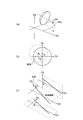
- (C) shows the amount of movement of the ball center by the first rotation. It is a figure which shows a mode that the light reception optical system has been arrange
- FIG. It is a figure which shows the flowchart of the example 1 of execution. It is a figure which shows the flowchart of the execution example 2.
- FIG. It is a figure which shows the flowchart of the measuring method of this embodiment. It is a figure which shows the mode of a movement of an irradiation position, (a) shows the position before the movement of one irradiation position, (b) shows the position after the movement of one irradiation position, (c) is the other The position before the movement of the irradiation position is shown, and (d) shows the position after the movement of the other irradiation position. It is a figure which shows the flowchart of the measuring method of this embodiment.
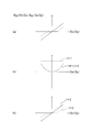
- FIG. 6 is a diagram showing an object height function appearing in decentering aberration sensitivities B 2jl (Ox, Oy) and B 3jl (Ox, Oy), where (a) shows a case where the optical system to be tested is not decentered, and (b) (C) shows a case where the optical system to be tested is decentered.
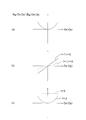
- FIG. 5 is a diagram showing an object height function appearing in decentration aberration sensitivity B 4jl (Ox, Oy), where (a) shows a case where the test optical system is not decentered, and (b) and (c) show the test optics. The case where the system is eccentric is shown.
- FIG. 6 is a diagram showing an object height function appearing in decentration aberration sensitivities B 5jl (Ox, Oy) and B 6jl (Ox, Oy), where (a) shows a case where the optical system to be tested is not decentered, and (b) (C) shows a case where the optical system to be tested is decentered.
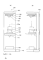
- FIG. 6 is a diagram showing an object height function appearing in decentering aberration sensitivities B 7jl (Ox, Oy) and B 8jl (Ox, Oy), where (a) shows a case where the optical system to be tested is not decentered, and (b) (C) shows a case where the optical system to be tested is decentered. It is a figure which shows the eccentricity measuring device of embodiment.
- FIG. 5A illustrates a case where the substrate is distorted
- FIG. 5B illustrates a case where the substrate is tilted
- FIG. 5C illustrates a case where an error occurs in the lens pitch.
- D shows a case where the focal lengths of the lenses are different.
- FIGS. 2A and 2B are diagrams illustrating a state in which the second rotation is performed, in which FIG. 2A illustrates a state before the holding member is moved, and FIG. 2B illustrates a state after the holding member is moved.
- FIG. 1 is a conceptual diagram showing how aberration occurs due to decentration. Since FIG. 1 is a conceptual diagram, the positions of the image IM1, the image IM2, and the image IM3, and the size and shape of the image are not accurate.
- the image IM1 is formed by the lens surface LS1
- the image IM2 is formed by the lens surface LS2
- the image IM3 is formed by the lens surface LS3.
- the image of the object point OB is formed by the lens surface LS1
- the formed image is relayed by the lens surface LS2 and the lens surface LS3.
- the lens surface LS1, the lens surface LS2, and the lens surface LS3 are decentered with respect to the optical axis.
- the image IM1, the image IM2, and the image IM3 are formed at positions away from the optical axis.
- aberration occurs in the image IM1 with the decentering of the lens surface LS1.
- This image IM1 corresponds to an object point on the lens surface LS2.
- the aberration in the image IM2 is obtained by adding the aberration generated by the decentering of the lens surface LS2 to the aberration in the image IM1.
- the aberration in the image IM3 is obtained by adding the aberration generated by the decentering of the lens surface LS3 to the aberration in the image IM2.
- the images are relayed while the aberrations generated on the lens surface LS1, the lens surface LS2, and the lens surface LS3 are added.
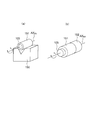
- FIG. 2 is a diagram for explaining the degree of freedom of eccentricity, in which (a) shows the degree of freedom of eccentricity on a spherical surface, and (b) and (c) show the degree of freedom of eccentricity on an aspherical surface.
- the eccentricity on the spherical surface can be expressed by the position of the spherical center.
- the degree of freedom of eccentricity on the spherical surface is geometrically only a shift in the X direction and a shift in the Y direction.
- the degree of freedom of eccentricity on the spherical surface may be considered as only the shift in the X direction and the shift in the Y direction.
- the gap between the faces also occurs during manufacturing.
- the deviation of the surface interval at the time of manufacture is, for example, an error in thickness for one lens and an error in lens interval for two lenses. In practice, it is not possible to distinguish the gap between the planes due to manufacturing errors and the gap between the planes when the spherical surface is tilted.
- the aspherical surface has an aspherical surface apex and an aspherical axis as shown in FIGS.
- the aspheric axis is a rotationally symmetric axis. Since an aspherical surface has this aspherical axis, in the case of an aspherical surface, there are a tilt in the A direction and a tilt in the B direction in addition to the shift in the X direction and the shift in the Y direction.
- the shift in the X direction and the shift in the Y direction are eccentric degrees of freedom with respect to the top of the aspheric surface. Further, the tilt in the A direction and the tilt in the B direction are degrees of freedom of eccentricity with respect to the aspherical axis.
- the number of degrees of freedom of eccentricity differs between spherical and aspherical surfaces. Therefore, for example, when the first surface of one lens is a spherical surface and the second surface is an aspheric surface, the number of degrees of freedom of eccentricity is six at the maximum.
- FIG. 3A and 3B are diagrams showing the coordinates in the measurement system and the decentration of the optical system to be tested.
- FIG. 3A is a diagram showing the decentration with a lens surface
- FIG. 3B is a diagram showing the decentration with a spherical center.
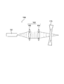
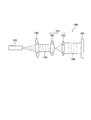
- the measurement system has a light projecting system and a light receiving system.
- the light projecting system is represented by the Ox axis, the Oy axis, and the Oz axis
- the light receiving system is represented by the ⁇ x axis and the ⁇ y axis.
- the coordinates of the light projecting system are represented by object height coordinates (Ox, Oy, Oz), and the coordinates of the light receiving system are represented by pupil coordinates ( ⁇ x, ⁇ y).
- the optical system to be measured is composed of a lens surface of the first lens surface LS 1 up to the j lens surface LS j.
- a situation is considered in which these lens surfaces are shifted in the Y direction with respect to the Oz axis.
- the lens surfaces are all spherical.
- the lens surface shift is represented using a spherical center.
- SC 1 , SC 2 ,..., SC j represent sphere centers of the lens surfaces.
- ⁇ 1 , ⁇ 2 ,..., ⁇ j represent the amount of shift in the Y direction of each lens surface.
- a light beam LB is irradiated onto the optical system to be measured from the object height coordinates (Ox, Oy) in the light projecting system.
- the light beam LB is emitted from the OxOy surface. Therefore, the object height coordinate is (Ox, Oy, 0) to be precise, but is (Ox, Oy) for simplicity.
- the light beam LB 'that has passed through the test optical system enters the light receiving system.
- the light beam LB indicates a part of the light beam originally irradiated on the optical system to be tested.
- the light beam LB ' indicates a part of the light beam that is originally incident on the light receiving system.
- wavefront data is acquired based on the light beam LB ′.
- the wavefront of the light beam LB ' has a wavefront aberration caused by the decentering. Therefore, by analyzing the wavefront data, it is possible to obtain wavefront aberration caused by decentration.
- the aberration generated in the rotationally symmetric optical system is a term that does not depend on the amount of eccentricity, a term that is proportional to the first power of the eccentricity amount, a term that is proportional to the square of the eccentricity amount, a term that is proportional to the third power of the eccentricity amount, A term proportional to the fourth power of the amount of decentering can be developed using a polynomial expression (see: third-order aberration theory of an optical system with decentration, third-order aberration theory of an eccentric optical system) Both, Japan Opto-Mechatronics Association, Image field distribution model of wavefront aberration and models of distortion and field curvature [T. Matsuzawa: J.Opt.Soc.Am.A, 28, No. 2 (2011) 96-110]).
- the wavefront aberration W can be expressed by, for example, the following formula (1).
- the wavefront aberration W here is described as a deviation from the wavefront when the optical system to be tested is not decentered.
- W (Ox, Oy, ⁇ x, ⁇ y, ⁇ 1 , ⁇ 2 , ..., ⁇ j ) ⁇ 1 B 11 (Ox, Oy, ⁇ x, ⁇ y) + ⁇ 1 2 B 12 (Ox, Oy, ⁇ x, ⁇ y) + ⁇ 2 B 21 (Ox, Oy, ⁇ x, ⁇ y) + ⁇ 2 2 B 22 (Ox, Oy, ⁇ x, ⁇ y) + ...
- ⁇ j is the amount of eccentricity with respect to the Oz axis in the j-th plane
- B j1 (Ox, Oy, ⁇ x, ⁇ y) is the decentration aberration sensitivity proportional to the first power of the decentration amount on the j-th plane
- B j2 (Ox, Oy, ⁇ x, ⁇ y) is the decentration aberration sensitivity proportional to the square of the decentration amount on the j-th plane
- each term of the polynomial is represented by the product of the amount of decentration and the sensitivity of decentration aberration.
- the amount of eccentricity is not limited to the amount of shift in the Y direction. Therefore, in terms of a general amount of eccentricity, the amount of eccentricity is represented by ⁇ instead of ⁇ .
- the wavefront aberration W is developed based on the aberration theory, but the expansion is up to a term proportional to the square of the eccentricity (a term proportional to ⁇ 2 ).
- a term proportional to ⁇ 2 a term proportional to ⁇ 2 .
- each term on the right side of Equation (1) is referred to as “aberration component”.
- a term multiplied by the amount of eccentricity ⁇ is referred to as “decentration aberration component”.
- centration aberration component Each term on the right side of Equation (1) is multiplied by an eccentricity amount ⁇ . Therefore, all the terms on the right side of Equation (1) are decentration aberration components.
- Table 1 shows the explanation of each term in the formula (1).
- the decentration aberration component in the expression (1) includes an eccentric aberration component proportional to the first power of the decentering amount (a term proportional to ⁇ ) and an eccentric aberration component proportional to the square of the decentering amount ( ⁇ 2 )).
- B j1 Ox, Oy, ⁇ x, ⁇ y
- B j2 Ox, Oy, ⁇ x, ⁇ y
- wavefront aberration can be obtained by analyzing wavefront data.
- the wavefront aberration can be developed by a polynomial of aberration components.
- the decentration aberration sensitivity in each aberration component can be developed by a polynomial based on the aberration theory.
- decentering aberration sensitivity B jl Ox, Oy, ⁇ x , ⁇ y
- B jl (Ox, Oy, ⁇ x , ⁇ y) 1 ⁇ B 1jl (Ox, Oy) + ⁇ x ⁇ B 2jl (Ox, Oy) + ⁇ y ⁇ B 3jl (Ox, Oy) + ⁇ 2 ( ⁇ x 2 + ⁇ y 2 ) -1 ⁇ B 4jl (Ox, Oy) + ⁇ x 2 - ⁇ y 2 ⁇ ⁇ B 5jl (Ox, Oy) + 2 ⁇ x ⁇ y ⁇ B 6jl (Ox, Oy) + ⁇ 3 ( ⁇ x 2 + ⁇ y 2 ) ⁇ x-2 ⁇ x ⁇ ⁇ B 7jl (Ox, Oy) + ⁇ 3 ( ⁇ x 2 + ⁇ y 2 ) ⁇ y-2 ⁇ y ⁇ B 8jl (Ox, Oy) + ⁇ 6 ( ⁇ x 2 + ⁇ y 2 ) 2 -6 ( ⁇ x 2 + ⁇ y 2 ) +1 ⁇ ⁇ B 9jl (Ox, Oy)
- B zjl (Ox, Oy)
- B zjl (Ox, Oy) is a decentering aberration sensitivity of terms first Z term of Zernike term is multiplied by the eccentric in the j surface This is the decentration aberration sensitivity proportional to the first power of the quantity.
- Table 2 shows the relationship between each term of the Zernike term, the function representing each term, and the aberration. Table 2 shows the correspondence between the first to ninth terms of the Zernike term.
- Each term of the Zernike term is expressed by pupil coordinates ⁇ x and ⁇ y.
- the order determined by the order at ⁇ x and the order at ⁇ y is the maximum order of the pupil coordinates. If this maximum order is an even order, the order of the function of that term is an even order. If the maximum order is an odd order, the order of the function of the term is an odd order.
- the function representing the second term of the Zernike term is a function of which the maximum degree of the pupil coordinates is the first order and the odd order.
- the pupil coordinates are ⁇ x ⁇ y, so the maximum degree of the pupil coordinates in the sixth term of the Zernike term is second order and even order. Therefore, the function representing the sixth term of the Zernike term is a function in which the maximum degree of pupil coordinates is second order and even order.
- Table 3 shows a summary of the first to ninth terms.
- Equation (2) The second term of Equation (2) is a term obtained by multiplying B 2jl (Ox, Oy) by ⁇ x. Therefore, the second term of Equation (2) is a term obtained by multiplying B 2jl (Ox, Oy) by a function having an odd-order pupil coordinate.
- the sixth term of Equation (2) is a term obtained by multiplying B 6jl (Ox, Oy) by ⁇ x ⁇ y. Therefore, the sixth term of Equation (2) is a term obtained by multiplying B 6jl (Ox, Oy) by a function having an even-order pupil coordinate.
- Table 4 shows an explanation of each term in the formula (2).
- decentering aberration sensitivity B jl (Ox, Oy, ⁇ x , ⁇ y) when deployed with Zernike polynomials, each term of the polynomial, the term pupil coordinate is multiplied by the odd order function, the pupil coordinate is an even number It is divided into a term multiplied by a function of order.
- the decentration aberration sensitivity B zjl (Ox, Oy) can also be developed by a polynomial expression.
- the expansion formula differs between a term multiplied by a function of odd-order pupil coordinates and a term multiplied by a function of even-order pupil coordinates.
- the decentration aberration sensitivity B zj1 (Ox, Oy) is the decentration aberration sensitivity of the term multiplied by the Z term of the Zernike term, and is decentered in proportion to the first power of the decentration amount on the j th surface. It represents the aberration sensitivity.
- Decentration aberration sensitivity B zj1 (Ox, Oy) of a term whose pupil coordinates are multiplied by an odd-order function will be described.
- This decentering aberration sensitivity B zj1 (Ox, Oy) is multiplied by the second term, the third term, the seventh term, the eighth term, etc. (hereinafter referred to as “the second term of the Zernike term, etc.”) of the Zernike term.
- the decentration aberration sensitivity of the given term is expressed by the following equation (3).
- B zj1 (Ox, Oy) C zj100 + C zj120 Ox 2 + C zj111 OxOy + C zj102 Oy 2 + (3)
- Equation (3) the decentration aberration sensitivity B zj1 (Ox, Oy) of the term multiplied by the second term of the Zernike term, etc. Is an even function.
- Decentration aberration sensitivity B zj1 (Ox, Oy) of a term whose pupil coordinates are multiplied by an even-order function will be described.
- This decentration aberration sensitivity B zj1 (Ox, Oy) is the first term, the fourth term, the fifth term, the sixth term, the ninth term, etc. of the Zernike term (referred to as “the fourth term of the Zernike term, etc.”). Is the decentration aberration sensitivity of the term multiplied by.
- the decentration aberration sensitivity B zj1 (Ox, Oy) of the term multiplied by the fourth term of the Zernike term is the object high coordinate. Is an odd function.
- the decentration aberration sensitivity B zj2 (Ox, Oy) is the decentration aberration sensitivity of the term multiplied by the Z term of the Zernike term, and is decentered in proportion to the square of the decentration amount on the j th surface. It represents the aberration sensitivity.
- Decentration aberration sensitivity B zj1 (Ox, Oy) of a term whose pupil coordinates are multiplied by an odd-order function will be described.
- the decentration aberration sensitivity B zj2 (Ox, Oy) is the decentration aberration sensitivity of a term multiplied by the second term of the Zernike term.
- the decentration aberration sensitivity B zj2 (Ox, Oy) of the term multiplied by the second term of the Zernike term is the object high coordinate. Is an odd function.
- Decentration aberration sensitivity B zj1 (Ox, Oy) of a term whose pupil coordinates are multiplied by an even-order function will be described.
- the decentration aberration sensitivity B zj2 (Ox, Oy) is the decentration aberration sensitivity of a term multiplied by the fourth term of the Zernike term.
- B zj2 (Ox, Oy) C zj200 + C zj220 Ox 2 + C zj211 OxOy + C zj202 Oy 2 + (6)
- the decentration aberration sensitivity B zj2 (Ox, Oy) of the term multiplied by the fourth term of the Zernike term is the object high coordinate. Is an even function.
- C in the equations (3) to (6) is a constant that does not depend on the object height coordinates, pupil coordinates, and eccentricity.
- the subscripts in C indicate the Z-th term of the Zernike term, the j-th surface, the value of l, the order at the object height coordinate Ox, and the order at the object height coordinate Oy in order from the left side.
- the decentration aberration sensitivity B zjl (Ox, Oy) is divided into an odd function for the object height coordinate and an even function for the object height coordinate, depending on conditions.
- aberration occurs due to the decentering of the lens surface in the test optical system.
- the generated aberration appears as wavefront aberration.
- the wavefront aberration is expressed by the amount of decentration and the decentration aberration sensitivity. Therefore, the amount of decentration can be obtained from the wavefront aberration and the decentration aberration sensitivity.
- the eccentricity measuring method of the present embodiment (hereinafter referred to as “the measuring method of the present embodiment”) will be described.
- the decentering amount measuring method of this embodiment is a method for measuring the amount of decentering by irradiating a test optical system arranged on a measurement axis with a light beam, and based on the light beam emitted from the test optical system.
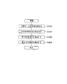
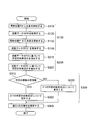
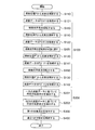
- FIG. 4 shows a flowchart of the measurement method of this embodiment.
- the measurement method of this embodiment is a method of measuring the amount of eccentricity by irradiating a test optical system arranged on a measurement axis with a light beam.
- the measurement method of the present embodiment includes step S100, step S200, step S300, and step S400.
- Step S100 is an acquisition process. As described above, the test optical system is irradiated with the light beam. The light beam applied to the test optical system passes through the test optical system and exits from the test optical system. In step S100, wavefront data WFD is acquired based on the light beam emitted from the test optical system.
- Step S200 is a first extraction process.
- a predetermined aberration component is extracted from the wavefront data WFD.
- This predetermined aberration component is an aberration component including an aberration component caused by decentration.
- the wavefront of the light beam emitted from the test optical system includes wavefront aberration caused by the decentering.
- the wavefront data WFD is not data indicating the wavefront aberration itself, but includes information on the wavefront aberration.
- Wavefront aberration is the sum of various types of aberrations.
- step S200 the amount of aberration in each aberration can be obtained by analyzing the wavefront data WFD.
- a polynomial is used.
- An example of the polynomial is a Zernike polynomial.
- the wavefront aberration W is developed using Zernike polynomials
- the wavefront aberration W is expressed by the following equation (7).
- the wavefront aberration is developed using up to the ninth term of the Zernike term.
- W (Ox, Oy, ⁇ x, ⁇ y, ⁇ 1 , ⁇ 2 , ..., ⁇ j ) 1 ⁇ W 1 (Ox, Oy, ⁇ 1 , ⁇ 2 , ..., ⁇ j ) + ⁇ x ⁇ W 2 (Ox, Oy, ⁇ 1 , ⁇ 2 , ..., ⁇ j ) + ⁇ y ⁇ W 3 (Ox, Oy, ⁇ 1 , ⁇ 2 , ..., ⁇ j ) + ⁇ 2 ( ⁇ x 2 + ⁇ y 2 ) -1 ⁇ ⁇ W 4 (Ox, Oy, ⁇ 1 , ⁇ 2 , ..., ⁇ j ) + ( ⁇ x 2 - ⁇ y 2 ) ⁇ W 5 (Ox, Oy, ⁇ 1 , ⁇ 2 , ..., ⁇ j ) + 2 ⁇ x ⁇ y ⁇ W 6 (Ox, Oy, ⁇ 1 , ⁇ 2 , ...,
- the wavefront aberration W M obtained by analyzing the wavefront data WFD is known. Therefore, by changing W 1 to W 9 in Equation (7), a combination of W 1 to W 9 that minimizes the difference between the wavefront aberration W and the wavefront aberration W M is obtained.
- Equation (2 ′) the eccentric aberration sensitivity B jl (Ox, Oy, ⁇ x , ⁇ y) can be expanded as shown in Equation (2 ').
- Equation (2 ′) the Zernike term is represented by f z ( ⁇ x, ⁇ y).
- Equation (2 ′) the Zernike term is represented by f z ( ⁇ x, ⁇ y).
- the description of the fifth to eighth terms and the tenth term or more of the Zernike term is omitted.
- B jl (Ox, Oy, ⁇ x , ⁇ y) f 1 ( ⁇ x, ⁇ y) ⁇ B 1jl (Ox, Oy) + f 2 ( ⁇ x, ⁇ y) ⁇ B 2jl (Ox, Oy) + f 3 ( ⁇ x, ⁇ y) ⁇ B 3jl (Ox, Oy) + f 4 ( ⁇ x, ⁇ y) ⁇ B 4jl (Ox, Oy) + ⁇ ⁇ ⁇ + f 9 ( ⁇ x, ⁇ y) ⁇ B 9jl (Ox, Oy) (2 ')
- formula (1-1) the first of the subscript f and the first subscript B represents the number of the Zernike term. Therefore, formula (1-2) is obtained by summing up for each Zernike term number.
- W (Ox, Oy, ⁇ x, ⁇ y, ⁇ 1 , ⁇ 2 , ..., ⁇ j ) f 1 ( ⁇ x, ⁇ y) ⁇ [ ⁇ 1 B 111 (Ox, Oy) + ⁇ 2 B 121 (Ox, Oy) + ⁇ ⁇ ⁇ + ⁇ j B 1j1 (Ox, Oy) ⁇ + ⁇ 1 2 B 112 (Ox, Oy) + ⁇ 2 2 B 122 (Ox, Oy) + ⁇ ⁇ ⁇ + ⁇ j 2 B 1j2 (Ox, Oy) ⁇ ] + f 2 ( ⁇ x, ⁇ y) ⁇ [ ⁇ 1 B 211 (Ox, Oy) + ⁇ 2 B 221 (Ox, Oy) + ⁇ ⁇
- the right sides of the equations (8-1) to (8-9) each include a term including ⁇ 1 to ⁇ j and a term including ⁇ 1 2 to ⁇ j 2 .
- W 1 to W 9 are all expressed using terms that are multiplied by the amount of eccentricity ⁇ .
- the term multiplied by the decentration amount ⁇ is the “decentration aberration component”
- W 1 to W 9 are all decentration aberration components.
- the predetermined aberration component is an aberration component including an aberration component caused by decentration.
- W 1 to W 9 are decentration aberration components, that is, aberration components generated by decentration. Therefore, W 1 to W 9 are predetermined aberration components.
- a predetermined aberration component can be extracted from the wavefront data WFD.
- Step S300 is a second extraction process.
- the first aberration component is extracted from the predetermined aberration component.
- This first aberration component is an aberration component proportional to the first power of the amount of decentration.
- W 1 to W 9 are predetermined aberration components.
- each of W 1 to W 9 is composed of an aberration component proportional to the first power of the decentering amount and an aberration component proportional to the second power of the decentering amount.
- the amount of decentration and the amount of aberration do not have a linear relationship.
- an aberration component proportional to the first power of the decentering amount that is, a first aberration component is extracted from predetermined aberration components.
- the first aberration component is obtained by removing the aberration component proportional to the square of the decentering amount from the equations (8-1) to (8-9). Accordingly, when the first aberration components are W 11 to W 91 , W 11 to W 91 are expressed by the following equations (9-1) to (9-9).
- W 11 (Ox, Oy, ⁇ 1 , ⁇ 2 , ..., ⁇ j ) ⁇ 1 B 111 (Ox, Oy) + ⁇ 2 B 121 (Ox, Oy) + ⁇ ⁇ ⁇ + ⁇ j B 1j1 (Ox, Oy) (9-1)
- W 21 (Ox, Oy, ⁇ 1 , ⁇ 2 , ..., ⁇ j ) ⁇ 1 B 211 (Ox, Oy) + ⁇ 2 B 221 (Ox, Oy) + ⁇ ⁇ ⁇ + ⁇ j B 2j1 (Ox, Oy) (9-2)
- W 31 (Ox, Oy, ⁇ 1 , ⁇ 2 , ..., ⁇ j ) ⁇ 1 B 311 (Ox, Oy) + ⁇ 2 B 321 (Ox, Oy) + ⁇ ⁇ ⁇ + ⁇ j B 3j1 (Ox, Oy) (9-3)
- W 11 ⁇ 1 B 111 + ⁇ 2 B 121 +... + ⁇ j B 1j1 (10-1)
- W 21 ⁇ 1 B 211 + ⁇ 2 B 221 +... + ⁇ j B 2j1 (10-2)
- W 31 ⁇ 1 B 311 + ⁇ 2 B 321 +... + ⁇ j B 3j1 (10-3)
- W 41 ⁇ 1 B 411 + ⁇ 2 B 421 +... + ⁇ j B 4j1 (10-4)
- W 51 ⁇ 1 B 511 + ⁇ 2 B 521 +...
- W 61 ⁇ 1 B 611 + ⁇ 2 B 621 + ⁇ ⁇ ⁇ + ⁇ j B 6j1 (10-6)
- W 71 ⁇ 1 B 711 + ⁇ 2 B 721 + ... + ⁇ j B 7j1 (10-7)
- W 81 ⁇ 1 B 811 + ⁇ 2 B 821 +... + ⁇ j B 8j1 (10-8)
- W 91 ⁇ 1 B 911 + ⁇ 2 B 921 + ⁇ ⁇ ⁇ + ⁇ j B 9j1 (10-9)
- Step S400 is an analysis process.
- simultaneous linear equations regarding the first aberration component, the decentration aberration sensitivity, and the decentering amount are analyzed.
- the relationship between the amount of decentration and the amount of aberration can be handled linearly. Further, if the relationship between the amount of decentration and the amount of aberration can be handled linearly, even if the amount of decentration of the optical system to be tested is large as a manufacturing error, the amount of decentration can be obtained with high accuracy by solving the simultaneous linear equations described later. it can.
- the unit of B 111 is “aberration amount / length” or “aberration amount / angle”.
- “Aberration amount / length” represents the amount of aberration generated when a single surface of the optical system to be tested is shifted by a unit decentering amount. “Aberration amount / angle” represents the amount of aberration that occurs when a single surface of the optical system under test is tilted by a unit eccentricity. Therefore, as described above, B 111 to B 9j1 represent the decentration aberration sensitivity.
- the decentration aberration sensitivity can be calculated based on data when the test optical system is designed. Then, in the equations (10-1) to (10-9), the first aberration component on the left side, that is, the aberration amount, and the decentration aberration sensitivity on the right side are known. Therefore, the eccentric amounts ⁇ 1 to ⁇ j can be obtained by solving the simultaneous linear equations (10-1) to (10-9).
- the first aberration component is an amount proportional to the first power of the decentering amount. Therefore, the decentration aberration sensitivity must also be an aberration sensitivity proportional to the first power of the decentration amount.
- the decentration aberration sensitivity proportional to the first power of the decentration amount is a change in decentration aberration per unit decentering amount of the aberration component proportional to the first power of the decentration amount.
- the acquisition of the wavefront data is performed using a light beam emitted from the test optical system. Therefore, the test optical system may be composed of one lens or a plurality of lenses.
- the lens surface may be spherical or aspherical. Moreover, since the eccentricity of the lens surface is not measured one by one, measurement can be performed in a short time.
- the eccentricity can be measured in a short time regardless of the shape of the lens surface and the number of lenses constituting the optical system.
- the measurement method of the present embodiment in the acquisition process, light beams are irradiated from two irradiation positions, the two irradiation positions are symmetric with respect to the measurement axis, and the first extraction process is performed at one irradiation position. It is preferable to extract a predetermined aberration component from each of the wavefront data and the wavefront data at the other irradiation position.
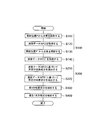
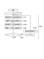
- FIG. 5 shows a flowchart of the measurement method of this embodiment.
- Step S100 includes Step S110, Step S120, Step S130, and Step S140.
- step S200 has step S210 and step S220.
- Step S100 is an acquisition process.
- the acquisition process includes step S110, step S120, step S130, and step S140.
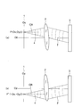
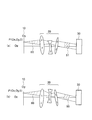
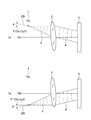
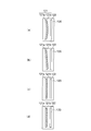
- FIGS. 6A and 6B are diagrams showing a state in which a test optical system is irradiated with a light beam.
- FIG. 6A shows irradiation from an irradiation position P
- FIG. 6B shows irradiation from an irradiation position P ′. .
- step S110 the light source is arranged at the irradiation position P of the light projecting system 1.
- the object height coordinate of the irradiation position P is (Ox, Oy, 0).
- a test light system 2 is irradiated with a light beam from a light source.
- a spherical wave 4 is emitted from the light source.
- the spherical wave 4 is incident on the test optical system 2. Since the test optical system 2 is decentered with respect to the Oz axis, a non-planar wave 7 is emitted from the test optical system 2.
- the Oz axis is a measurement axis.
- step S120 wavefront data WFD is acquired.
- the non-planar wave 7 emitted from the test optical system 2 enters the light receiving system 3. Therefore, wavefront data WFD is acquired by the light receiving system 3.
- step S130 a light source is arranged at the irradiation position P ′ of the light projecting system 1.
- the object height coordinate of the irradiation position P ′ is ( ⁇ Ox, ⁇ Oy, 0).
- a test light system 2 is irradiated with a light beam from a light source.
- a non-planar wave 7 ′ is emitted from the test optical system 2.
- step S140 wavefront data WFD 'is acquired.
- the non-planar wave 7 ′ emitted from the test optical system 2 enters the light receiving system 3. Therefore, the wavefront data WFD ′ is acquired by the light receiving system 3.
- the irradiation position P and the irradiation position P ′ are symmetric with respect to the measurement axis.
- each lens surface of the test optical system is decentered with respect to the measurement axis. Therefore, the optical path passing through the optical system to be measured is asymmetrical between the beam irradiated from the irradiation position P and the beam irradiated from the irradiation position P ′.
- the non-planar wave 7 and the non-planar wave 7 ′ do not have a symmetrical wavefront shape. Therefore, the wavefront data WFD and the wavefront data WFD ′ are not symmetric data.
- Step S200 is a first extraction process.
- Step S200 includes steps S210 and S220.
- the wavefront data WFD and the wavefront data WFD ′ are not symmetric data.
- step S210 a predetermined aberration component is extracted from the wavefront data WFD at the irradiation position P.
- a predetermined aberration component is extracted from the wavefront data WFD 'at the irradiation position P'.
- step S300 the first aberration component is extracted.
- Step S400 is executed using the extracted first aberration component.
- the eccentricity amounts ⁇ 1 to ⁇ j can be obtained.
- the eccentricity can be measured in a short time regardless of the shape of the lens surface and the number of lenses constituting the optical system.
- the predetermined aberration component includes the second aberration component
- the second aberration component is an aberration component proportional to the square of the decentering amount of the predetermined aberration component.
- the object height coordinate is a coordinate representing the irradiation position
- the predetermined function is a function representing the second aberration component and includes the object height coordinate as a variable
- the second extraction step includes: A first calculation step and a second calculation step.
- the first calculation step when the predetermined function is an odd function, the predetermined aberration component at one irradiation position and the predetermined calculation at the other irradiation position.
- the second calculation step when the predetermined function is an even function, the difference between the predetermined aberration component at one irradiation position and the predetermined aberration component at the other irradiation position is calculated. It is preferable to take.
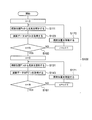
- FIG. 7 shows a flowchart of the measurement method of this embodiment.
- Step S100 includes Step S110, Step S120, Step S130, and Step S140.
- step S200 has step S210 and step S220.
- Step S300 includes step S310, step S320, and step S330. Detailed description of step S100 and step S200 is omitted.
- the optical system is irradiated with the light beam from two irradiation positions that are symmetrical with respect to the measurement axis.
- a predetermined aberration component is extracted from each of the wavefront data WFD and the wavefront data WFD '(step S200).
- the object height coordinate of one irradiation position P is (Ox, Oy)
- the object height coordinate of the other irradiation position P ' is (-Ox, -Oy).
- the wavefront aberration W is obtained by analyzing the wavefront data WFD.
- the predetermined aberration components W 1 to W 9 extracted from the wavefront aberration W are expressed by the above equations (8-1) to (8-9). ).
- the wavefront aberration W is acquired by analyzing the wavefront data WFD ′.
- the irradiation position P ′ object height coordinate is ( ⁇ Ox, ⁇ Oy)
- the predetermined aberration components W 1 to W 9 extracted from the wavefront aberration W are expressed by the following equations (8-1 ′) to ( 8-9 ′).
- W 1 (-Ox, -Oy, ⁇ 1 , ⁇ 2 , ..., ⁇ j ) [ ⁇ 1 B 111 (-Ox, -Oy) + ⁇ 2 B 121 (-Ox, -Oy) + ⁇ ⁇ ⁇ + ⁇ j B 1j1 (-Ox, -Oy) ⁇ + ⁇ 1 2 B 112 ( ⁇ Ox, ⁇ Oy) + ⁇ 2 2 B 122 ( ⁇ Ox, ⁇ Oy) +...
- W 2 (-Ox, -Oy, ⁇ 1 , ⁇ 2 , ..., ⁇ j ) [ ⁇ 1 B 211 (-Ox, -Oy) + ⁇ 2 B 221 (-Ox, -Oy) + ⁇ ⁇ ⁇ + ⁇ j B 2j1 (-Ox, -Oy) ⁇ + ⁇ 1 2 B 212 ( ⁇ Ox, ⁇ Oy) + ⁇ 2 2 B 222 ( ⁇ Ox, ⁇ Oy) +...
- W 7 (-Ox, -Oy, ⁇ 1 , ⁇ 2 , ..., ⁇ j ) [ ⁇ 1 B 711 (-Ox, -Oy) + ⁇ 2 B 721 (-Ox, -Oy) + ⁇ ⁇ ⁇ + ⁇ j B 7j1 (-Ox, -Oy) ⁇ + ⁇ 1 2 B 712 (-Ox, -Oy) + ⁇ 2 2 B 722 (-Ox, -Oy) + ...
- W 8 ( ⁇ Ox, ⁇ Oy, ⁇ 1 , ⁇ 2 ,..., ⁇ j ) [ ⁇ 1 B 811 (-Ox, -Oy) + ⁇ 2 B 821 (-Ox, -Oy) + ⁇ ⁇ ⁇ + ⁇ j B 8j1 (-Ox, -Oy) ⁇ + ⁇ 1 2 B 812 ( ⁇ Ox, ⁇ Oy) + ⁇ 2 2 B 822 ( ⁇ Ox, ⁇ Oy) +...
- Step S300 is a second extraction step.
- the second extraction step that is, the step of extracting the first aberration component will be described.
- description will be made using the following predetermined aberration components.
- W 2 (Ox, Oy, ⁇ 1 , ⁇ 2 ,..., ⁇ j ) and W 2 ( ⁇ Ox, ⁇ Oy, ⁇ 1 , ⁇ 2 ,..., ⁇ j ) are respectively expressed by equations (8 ⁇ 2) and the formula (8-2 ′).
- W 2 (Ox, Oy, ⁇ 1 , ⁇ 2 , ..., ⁇ j ) [ ⁇ 1 B 211 (Ox, Oy) + ⁇ 2 B 221 (Ox, Oy) + ⁇ ⁇ ⁇ + ⁇ j B 2j1 (Ox, Oy) ⁇ + ⁇ 1 2 B 212 (Ox, Oy) + ⁇ 2 2 B 222 (Ox, Oy) + ⁇ ⁇ ⁇ + ⁇ j 2 B 2j2 (Ox, Oy) ⁇ ] (8-2)
- W 2 (-Ox, -Oy, ⁇ 1 , ⁇ 2 , ..., ⁇ j ) [ ⁇ 1 B 211 (-Ox, -Oy) + ⁇ 2 B 221 (-Ox, -Oy) + ⁇ ⁇ ⁇ + ⁇ j B 2j1 (-Ox, -Oy) ⁇ + ⁇ 1 2 B 212 ( ⁇ Ox, ⁇ Oy) + ⁇ 2 2
- W 2 includes an aberration component that is proportional to the first power of the decentering amount and an aberration component that is proportional to the second power of the decentering amount.
- the aberration component proportional to the first power of the decentering amount is the first aberration component
- the aberration component proportional to the second power of the decentering amount is the second aberration component. Accordingly, the first aberration component is W 21 and the second aberration component is W 22 .
- Table 5 shows the terms in the first aberration component W 21 for the expressions (8-2) and (8-2 ′).
- W 21 is represented only by the object height coordinates.
- Table 6 shows the terms in the second aberration component W 22 for the expressions (8-2) and (8-2 ′).
- B 2j1 (Ox, Oy) and B 2j1 ( -Ox , -Oy) in Table 5 are the decentration aberration sensitivities of the term multiplied by the second term of the Zernike term, and are the first power of the decentration amount on the j-th surface.
- the decentration aberration sensitivity proportional to is expressed.
- B 2j1 (Ox, Oy) and B 2j1 ( ⁇ Ox , ⁇ Oy) are expressed by equations (3 ′) and (3 ′′) as follows from equation (3).
- B 2j1 (Ox, Oy) C 2j100 + C 2j120 Ox 2 + C 2j111 OxOy + C 2j102 Oy 2 + ... (3 ')
- B 2j1 ( -Ox , -Oy) C 2j100 + C 2j120 Ox 2 + C 2j111 OxOy + C 2j102 Oy 2 + ... (3 ”)
- B 2j2 (Ox, Oy) and B 2j2 ( -Ox , -Oy) in Table 6 are the decentration aberration sensitivity of the term multiplied by the second term of the Zernike term, and the amount of decentration on the j-th surface. It shows the decentration aberration sensitivity proportional to the square.
- B 2j2 (Ox, Oy) and B 2j2 ( ⁇ Ox , ⁇ Oy) are expressed by the following equations (5 ′) and (5 ′′) from the equation (5).
- B 2j2 (Ox, Oy) C 2j210 Ox + C 2j201 Oy + C 2j230 Ox 3 + C 2j221 Ox 2 Oy + C 2j212 OxOy 2 + C 2j203 Oy 3 + ...
- B 2j1 (-Ox, -Oy) B 2j1 (Ox, Oy) of the first aberration component W 21 when the reflecting shown in Table 7.
- W 21 ( ⁇ Ox, ⁇ Oy) W 21 (Ox, Oy).
- the first aberration component W 21 is an even function with respect to the object height coordinate.
- B 2j2 (-Ox, -Oy) - shows B 2j2 (Ox, Oy) of the second aberration component W 22 when the reflected in Table 8.
- W 22 ( ⁇ Ox, ⁇ Oy) ⁇ W 22 (Ox, Oy).
- the second aberration component W 22 is an odd function with respect to the object height coordinate.
- W 4 (Ox, Oy, ⁇ 1, ⁇ 2, ⁇ , ⁇ j) and W 4 (-Ox, -Oy, ⁇ 1, ⁇ 2, ⁇ , ⁇ j) respectively, wherein (8-4) and (8-4 ′).
- W 4 (Ox, Oy, ⁇ 1 , ⁇ 2 , ..., ⁇ j ) [ ⁇ 1 B 411 (Ox, Oy) + ⁇ 2 B 421 (Ox, Oy) + ⁇ ⁇ ⁇ + ⁇ j B 4j1 (Ox, Oy) ⁇ + ⁇ 1 2 B 412 (Ox, Oy) + ⁇ 2 2 B 422 (Ox, Oy) + ⁇ ⁇ ⁇ + ⁇ j 2 B 4j2 (Ox, Oy) ⁇ ] (8-4)
- W 4 (-Ox, -Oy, ⁇ 1 , ⁇ 2 , ..., ⁇ j ) [ ⁇ 1 B 411 (-Ox, -Oy) + ⁇ 2 B 421 (-Ox, -Oy) + ⁇ ⁇ ⁇ + ⁇ j B 4j1 (-Ox, -Oy) ⁇ + ⁇ 1 2 B 412 ( ⁇ Ox, ⁇ Oy) + ⁇ 2 2
- W 4 includes an aberration component that is proportional to the first power of the decentering amount and an aberration component that is proportional to the second power of the decentering amount.
- the aberration component proportional to the first power of the decentering amount is the first aberration component
- the aberration component proportional to the second power of the decentering amount is the second aberration component. Therefore, the first aberration component is W 41 , and the second aberration component is W 42 .
- Table 9 shows the terms in the first aberration component W 41 for the expressions (8-4) and (8-4 ′).
- W 41 is represented only by the object height coordinates.
- Table 10 shows the terms in the second aberration component W 42 for the expressions (8-4) and (8-4 ′).
- B 4j1 (Ox, Oy) and B 4j1 ( -Ox , -Oy) in Table 10 are the decentration aberration sensitivity of the term multiplied by the fourth term of the Zernike term, and are the first power of the decentering amount on the j-th surface.
- the decentration aberration sensitivity proportional to is expressed.
- B 4j1 (Ox, Oy) and B 4j1 ( ⁇ Ox , ⁇ Oy) are expressed by equations (4 ′) and (4 ′′) as follows from equation (4).
- B 4j1 (Ox, Oy) C 4j110 Ox + C 4j101 Oy + C 4j130 Ox 3 + C 4j121 Ox 2 Oy + C 4j112 OxOy 2 + C 4j103 Oy 3 + ...
- B 4j2 (Ox, Oy) and B 4j2 ( -Ox , -Oy) in Table 11 are the decentration aberration sensitivity of the term multiplied by the fourth term of the Zernike term, and the amount of decentration on the j-th surface. It shows the decentration aberration sensitivity proportional to the square.
- B 4j2 (Ox, Oy) and B 4j2 ( ⁇ Ox , ⁇ Oy) are expressed by the following equations (6 ′) and (6 ′′) from the equation (6).
- B 4j2 (Ox, Oy) C 4j200 + C 4j220 Ox 2 + C 4j211 OxOy + C 4j202 Oy 2 + ...
- B 4j2 ( -Ox , -Oy) C 4j200 + C 4j220 Ox 2 + C 4j211 OxOy + C 4j202 Oy 2 + ... (6 ”)
- B 4j1 (-Ox, -Oy) - B 4j1 (Ox, Oy) of the first aberration component W 41 when the reflecting shown in Table 11.
- W 41 ( ⁇ Ox, ⁇ Oy) ⁇ W 41 (Ox, Oy).
- the first aberration component W 41 is an odd function with respect to the object height coordinate.
- B 4j2 (-Ox, -Oy) B 4j2 (Ox, Oy) of the second aberration component w 42 when reflected in Table 12.
- W 42 ( ⁇ Ox, ⁇ Oy) W 42 (Ox, Oy).
- the function representing the first aberration component W 21 is an even function and the function representing the first aberration component W 22 is an odd function.
- the function representing the first aberration component W 41 is an even function and the function representing the first aberration component W 42 is an odd function.
- the predetermined function is a function representing the second aberration component and the object height coordinate is a variable
- the predetermined function is divided into an even function and an odd function.
- step S310 is executed, and different operations are performed depending on whether the predetermined function is an odd function or the predetermined function is an even function.
- step S320 is executed. Step S320 is a first calculation step.
- the sum of the predetermined aberration component at one irradiation position and the predetermined aberration component at the other irradiation position is taken. That is, the sum of W 2 (Ox, Oy, ⁇ 1 , ⁇ 2 ,..., ⁇ j ) and W 2 ( ⁇ Ox, ⁇ Oy, ⁇ 1 , ⁇ 2 ,..., ⁇ j ) is taken.
- the first aberration component W 21 is expressed by Expression (9-2).
- Formula (9-2) is shown again below.
- W 21 (Ox, Oy, ⁇ 1 , ⁇ 2 , ..., ⁇ j ) ⁇ 1 B 211 (Ox, Oy) + ⁇ 2 B 221 (Ox, Oy) + ⁇ ⁇ ⁇ + ⁇ j B 2j1 (Ox, Oy) (9-2)
- Expression (11 ′) is obtained from Expression (11) and Expression (9-2).
- the first aberration component W 21 As shown in Expression (11 ′), by taking the sum of the two, the first aberration component W 21 remains and the second aberration component W 22 disappears. Therefore, the first aberration component W 21 can be extracted from the predetermined aberration component W 2 .
- step S330 is executed. Step S330 is a second calculation step.
- the difference between the predetermined aberration component at one irradiation position and the predetermined aberration component at the other irradiation position is taken. That is, the difference between W 4 (Ox, Oy, ⁇ 1 , ⁇ 2 ,..., ⁇ j ) and W 4 ( ⁇ Ox, ⁇ Oy, ⁇ 1 , ⁇ 2 ,..., ⁇ j ) is taken.
- the result of taking the difference between the two is shown in equation (12).
- W 4 (Ox, Oy, ⁇ 1 , ⁇ 2 ,..., ⁇ j ) ⁇ W 4 ( ⁇ Ox, ⁇ Oy, ⁇ 1 , ⁇ 2 ,..., ⁇ j ) 2 ⁇ ⁇ 1 B 411 (Ox, Oy) + ⁇ 2 B 421 (Ox, Oy) + ⁇ ⁇ ⁇ + ⁇ j B 4j1 (Ox, Oy) ⁇ (12)
- the first aberration component W 41 is expressed by Expression (9-4).
- Formula (9-4) is shown again below.
- W 41 (Ox, Oy, ⁇ 1 , ⁇ 2 , ..., ⁇ j ) ⁇ 1 B 411 (Ox, Oy) + ⁇ 2 B 421 (Ox, Oy) + ⁇ ⁇ ⁇ + ⁇ j B 4j1 (Ox, Oy) (9-4)
- Expression (12 ′) is obtained from Expression (12) and Expression (9-4).
- the first aberration component W 41 As shown in the equation (12 ′), by taking the difference between the two, the first aberration component W 41 remains and the second aberration component W 42 disappears. Therefore, the first aberration component W 41 can be extracted from the predetermined aberration component W 4 .
- Table 13 shows a summary of a case where the first aberration component W z1 and the second aberration component W z2 are an even function with respect to the object height coordinate and an odd function with respect to the object height coordinate.
- the first aberration component is represented by W z1
- the second aberration component is represented by W z2 .
- the first aberration component can be extracted from the predetermined aberration component by executing the first calculation step.
- W 3 (Ox, Oy, ⁇ 1 , ⁇ 2 ,..., ⁇ j ) and W 3 ( ⁇ Ox, ⁇ Oy, ⁇ 1 , ⁇ 2 ,..., ⁇ j ).
- W 7 (Ox, Oy, ⁇ 1 , ⁇ 2 ,..., ⁇ j ) and W 7 ( ⁇ Ox, ⁇ Oy, ⁇ 1 , ⁇ 2 ,..., ⁇ j ).
- W 8 (Ox, Oy, ⁇ 1 , ⁇ 2 ,..., ⁇ j ) and W 8 ( ⁇ Ox, ⁇ Oy, ⁇ 1 , ⁇ 2 ,..., ⁇ j ).
- Wz (Ox, Oy, ⁇ 1 , ⁇ 2, ⁇ , ⁇ j) + Wz (-Ox, -Oy, ⁇ 1, ⁇ 2, ⁇ , ⁇ j) 2 ⁇ 1 B z11 (Ox, Oy) + ... + 2 ⁇ j B zj1 (Ox, Oy)
- the first aberration component can be extracted from the predetermined aberration component by executing the second calculation step.
- W 9 (Ox, Oy, ⁇ 1 , ⁇ 2 ,..., ⁇ j ) and W 9 ( ⁇ Ox, ⁇ Oy, ⁇ 1 , ⁇ 2 ,..., ⁇ j ).
- Wz (Ox, Oy, ⁇ 1 , ⁇ 2, ⁇ , ⁇ j) -Wz (-Ox, -Oy, ⁇ 1, ⁇ 2, ⁇ , ⁇ j) 2 ⁇ 1 B z11 (Ox, Oy) + ... + 2 ⁇ j B zj1 (Ox, Oy)
- the first calculation step is performed.
- the sum of the predetermined aberration component at one irradiation position and the predetermined aberration component at the other irradiation position is taken.
- the first aberration component can be extracted from the predetermined aberration component.
- the second calculation step is performed.
- the difference between the predetermined aberration component at one irradiation position and the predetermined aberration component at the other irradiation position is taken.
- the first aberration component can be extracted from the predetermined aberration component.
- the first aberration component is extracted by executing step S300.
- Step S400 is executed using the extracted first aberration component.
- the eccentric amounts ⁇ 1 to ⁇ j can be obtained.
- the eccentricity can be measured in a short time regardless of the shape of the lens surface and the number of lenses constituting the optical system.
- the first aberration component can be extracted from the predetermined aberration component even when the design aberration component exists.
- the wavefront aberration W is a deviation from the wavefront when the test optical system is not decentered.
- the wavefront aberration W is described as a deviation from an ideal wavefront such as a plane wave or a spherical wave.
- the design aberration component will be described.
- the test optical system in the decentration measurement is an assembled lens, a group single unit, a lens single unit, or the like.
- the test optical system is manufactured based on design data.
- designing an optical system a plurality of lenses are combined so as to suppress the generation of aberration as much as possible. However, it is very difficult to reduce the generation amount of all aberrations to zero.
- some of the assembled lenses for example, each group alone and each lens alone generate aberrations in design.
- the test optical system has an aberration at the design stage. Therefore, if this aberration is a design aberration, the design aberration is also included in the wavefront aberration.
- the design aberration component is M (Ox, Oy, ⁇ x, ⁇ y)
- the wavefront aberration W is expressed by the following equation (1-3).
- W (Ox, Oy, ⁇ x, ⁇ y, ⁇ 1 , ⁇ 2 , ..., ⁇ j ) M (Ox, Oy, ⁇ x, ⁇ y) + ⁇ 1 B 11 (Ox, Oy, ⁇ x, ⁇ y) + ⁇ 1 2 B 12 (Ox, Oy, ⁇ x, ⁇ y) + ⁇ 2 B 21 (Ox, Oy, ⁇ x, ⁇ y) + ⁇ 2 2 B 22 (Ox, Oy, ⁇ x, ⁇ y) + ... + ⁇ j B j1 (Ox, Oy, ⁇ x, ⁇ y) + ⁇ j 2 B j2 (Ox, Oy, ⁇ x, ⁇ y) (1-3)
- the designed aberration component M (Ox, Oy, ⁇ x, ⁇ y) is a predetermined aberration component.
- the design aberration component M (Ox, Oy, ⁇ x, ⁇ y) can also be developed as a polynomial based on the aberration theory, similarly to the decentration aberration sensitivity. For example, when the Zernike polynomial is used, the design aberration component M (Ox, Oy, ⁇ x, ⁇ y) can be expanded by a polynomial as shown in the following equation (13).
- M (Ox, Oy, ⁇ x, ⁇ y) 1 ⁇ M 1 (Ox, Oy) + ⁇ x ⁇ M 2 (Ox, Oy) + ⁇ y ⁇ M 3 (Ox, Oy) + ⁇ 2 ( ⁇ x 2 + ⁇ y 2 ) -1 ⁇ ⁇ M 4 (Ox, Oy) + ⁇ x 2 - ⁇ y 2 ⁇ ⁇ M 5 (Ox, Oy) + 2 ⁇ x ⁇ y ⁇ M 6 (Ox, Oy) + ⁇ 3 ( ⁇ x 2 + ⁇ y 2 ) ⁇ x-2 ⁇ x ⁇ ⁇ M 7 (Ox, Oy) + ⁇ 3 ( ⁇ x 2 + ⁇ y 2 ) ⁇ y-2 ⁇ y ⁇ ⁇ M 8 (Ox, Oy) + ⁇ 6 ( ⁇ x 2 + ⁇ y 2 ) 2 -6 ( ⁇ x 2 + ⁇ y 2 ) +1 ⁇ ⁇ M 9 (Ox, Oy) + ... (13) here, M 1 (Ox, Oy) to M
- M z (Ox, Oy) is a function that depends on the object height coordinate and is multiplied by the Z term of the Zernike term. It is a function in the term.
- the Zernike term is a function that depends on the pupil coordinates. Therefore, M z (Ox, Oy) is a function that depends on the object height coordinate, and can be said to be a function in a term multiplied by a function that depends on the pupil coordinate.
- each term of the polynomial is a term multiplied by a function whose pupil coordinate is an odd order, and the pupil coordinate is an even order. And the term multiplied by the function.
- the function M z (Ox, Oy) depending on the object height coordinate can also be expanded by a polynomial.
- the expansion formula differs between a term multiplied by a function of odd-order pupil coordinates and a term multiplied by a function of even-order pupil coordinates.
- M z (Ox, Oy) C zm10 Ox + C zm01 Oy + C zm30 Ox 3 + zm21 Ox 2 Oy + C zm12 OxOy 2 + C zm03 Oy 3 + (14)
- M z (Ox, Oy) of a term multiplied by the second term of the Zernike term is an odd function with respect to the object high coordinate.
- M z (Ox, Oy) C zm00 + C zm20 Ox 2 + C zm11 OxOy + C zm02 Oy 2 + (15)
- M z (Ox, Oy) of a term multiplied by the fourth term of the Zernike term is an even function with respect to the object high coordinate.
- function representing the first aberration component the function representing the second aberration component, and the function depending on the object height coordinate in the design aberration component (hereinafter referred to as “function representing the design aberration component”) become an even function;
- Table 14 shows the result of summarizing the case of an odd function.
- the predetermined function that is, the function representing the second aberration component is an odd function
- the first calculation step when the first calculation step is performed, the second aberration component disappears.
- the function representing the second aberration component when the function representing the second aberration component is an odd function, the function representing the design aberration component is also an odd function. For this reason, when the first calculation step is performed, the design aberration component also disappears. As a result, the first aberration component can be extracted from the predetermined aberration component.
- the second aberration component disappears when the second calculation step is performed.
- the function representing the second aberration component is an even function
- the function representing the design aberration component is also an even function.
- the design aberration component also disappears.
- the first aberration component can be extracted from the predetermined aberration component.
- Step S400 is executed using the extracted first aberration component.
- the eccentric amounts ⁇ 1 to ⁇ j can be obtained.
- the decentering amount measuring method of the present embodiment even when there is a design aberration in the test optical system, it is short regardless of the shape of the lens surface and the number of lenses constituting the optical system.
- the amount of eccentricity can be measured over time.
- the acquisition step includes a first rotation.
- the optical system to be measured is rotated around the measurement axis, and the same irradiation position is used before the first rotation. It is preferable to acquire the wavefront data and the wavefront data after the first rotation.
- FIG. 8 shows a flowchart of the measurement method of this embodiment.
- step S100 includes step S110, step S121, step S122, and step S150.
- step S200, step S300, and step S400 are omitted.
- the wavefront data is data including information on wavefront aberration.
- Wavefront data is acquired by the light receiving system.
- the wavefront data is phase data.
- the light receiving system is a Shack-Hartmann sensor (hereinafter referred to as “SH sensor”)
- SH sensor Shack-Hartmann sensor
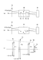
- FIGS. 9A and 9B are diagrams for explaining system aberrations in the light projection system.
- FIG. 9A shows a state where no system aberration occurs
- FIG. 9B shows a state where system aberrations occur in the light projection system.
- System aberration is an aberration of the measurement system itself. System aberration occurs in a light projecting system and a light receiving system.
- a light source is disposed at the irradiation position P of the light projecting system 10.
- the spherical wave 40 is emitted from the light source.
- the spherical wave 40 enters the test optical system 20. Since the test optical system 20 is decentered with respect to the Oz axis, a non-planar wave 50 is emitted from the test optical system 20.
- the wavefront of the light beam applied to the optical system 20 to be tested becomes a distorted wavefront 60, as shown in FIG.
- the non-planar wave 51 emitted from the test optical system 20 is different from the non-plane wave 50 when the spherical optical wave 40 is irradiated on the test optical system 20.
- FIG. 10A and 10B are diagrams showing system aberrations in the light receiving system, in which FIG. 10A shows system aberrations in the sensor component constituting unit, and FIG. 10B shows system aberrations in the wavefront data acquiring unit.
- the light receiving system 30 is composed of, for example, a sensor component configuration unit 31 and a wavefront data acquisition unit 32.
- the non-planar wave 50 that has entered the light receiving system 30 reaches the wavefront data acquisition unit 32 after passing through the sensor component component 31.
- the sensor system component 31 is provided with an optical system as necessary. For example, when it is necessary to make the diameter of the light beam incident on the light receiving system substantially coincide with the light receiving area in the wavefront data acquisition unit 32, the optical system is arranged in the sensor component constituting unit 31. In addition, an optical system is arranged in the sensor component constituent unit 31 when forming a plurality of light spot images.
- interference fringes are formed in the wavefront data acquisition unit 32.
- the light receiving system 30 is an SH sensor, a plurality of light spot images are formed in the wavefront data acquisition unit 32.
- the wavefront data acquisition unit 32 acquires the wavefront information by dividing the interference fringes into fine regions.
- the wavefront data acquisition unit 32 detects the positions of a plurality of light spot images. Therefore, in the wavefront data acquisition unit 32, for example, minute light receiving elements 33 (hereinafter referred to as “light receiving elements”) are two-dimensionally arranged.
- the light receiving elements 33 are not regularly arranged. Therefore, system aberration occurs in the wavefront data acquisition unit 32. Further, the size of the light receiving area of the light receiving element 33 may vary due to manufacturing errors. Also in this case, system aberration occurs in the wavefront data acquisition unit 32.
- the system aberration is also included in the wavefront aberration.
- the wavefront data acquired by the light receiving system 30 is not data that accurately reflects the wavefront aberration caused by the eccentricity of the test optical system 20.
- the wavefront aberration W is expressed by the following equation (1-4).
- the wavefront aberration W here is described as a deviation from the wavefront when there is no decentering of the test optical system and no system aberration.
- W (Ox, Oy, ⁇ x, ⁇ y, ⁇ 1 , ⁇ 2 , ..., ⁇ j ) Sys (Ox, Oy, ⁇ x, ⁇ y) + ⁇ 1 B 11 (Ox, Oy, ⁇ x, ⁇ y) + ⁇ 1 2 B 12 (Ox, Oy, ⁇ x, ⁇ y) + ⁇ 2 B 21 (Ox, Oy, ⁇ x, ⁇ y) + ⁇ 2 2 B 22 (Ox, Oy, ⁇ x, ⁇ y) + ... + ⁇ j B j1 (Ox, Oy, ⁇ x, ⁇ y) + ⁇ j 2 B j2 (Ox, Oy, ⁇ x, ⁇ y) (1-4)
- FIG. 11 is a diagram showing a method for obtaining a system aberration component in advance. Here, it is assumed that system aberration occurs in the sensor component component 31.
- an optical system 21 with very little aberration is used.
- the light beam emitted from the optical system 21 is in a state in which the angle, position, and light beam diameter incident on the light receiving system 30 coincide with the light beam emitted from the optical system 20 to be tested (FIG. 10A). Yes. That is, the irradiation position P P , the irradiation angle, the position of the optical system 21, and the inclination of the optical system 21 with respect to the Oz axis are adjusted so as to achieve such a state.
- the light source is arranged at the irradiation position P P (0x p , 0y p , 0) of the light projecting system 10. Since no system aberration occurs in the light projecting system 10, the spherical wave 40 is emitted from the light source. The spherical wave 40 is incident on the optical system 21. The optical system 21 is an optical system with very little aberration. Therefore, the plane wave 53 is emitted from the optical system 21. The plane wave 53 is incident on the sensor component component 31.
- system aberration in the sensor component component 31 is added to the plane wave 53.
- the non-planar wave 54 is emitted from the sensor component component 31.
- the non-planar wave 54 enters the wavefront data acquisition unit 32, and wavefront data is acquired.
- the acquired wavefront data includes only system aberration information in the sensor component component 31. Therefore, the wavefront aberration W ′ obtained from this wavefront data is expressed by the following equation (16).
- W ′ (Ox, Oy, ⁇ x, ⁇ y) Sys (Ox, Oy, ⁇ x, ⁇ y) (16)
- the light beam emitted from the optical system 21 is such that the angle, position, and light beam diameter incident on the light receiving system 30 coincide with the light beam emitted from the test optical system 20 (FIG. 10A). It has become. Therefore, the irradiation position P P (0x p , 0y p , 0) of the light projecting system 10 in FIG. 11 corresponds to the irradiation position P (0x, 0y, 0) in FIG. Therefore, the object height coordinate of W ′ is represented by (0x, 0y).
- Sys (Ox, Oy, ⁇ x, ⁇ y) can be removed by performing the calculation of Expression (17).
- This method can be easily implemented when there is only one irradiation position. However, if the number of irradiation positions becomes very large, the number of data to be obtained in advance becomes enormous. Therefore, it is not easy to implement this method.
- step S100 is executed as shown in FIG.
- FIG. 12 is a diagram showing the first rotation, where (a) shows a state before the first rotation, and (b) shows a state after the first rotation. It is assumed that both the light projecting system and the light receiving system have system aberrations.
- step S110 as shown in FIG. 12A, the test optical system 20 is irradiated with the light beam from the irradiation position P (Ox, Oy, 0).
- the wavefront 60 is incident on the test optical system 20.
- a non-planar wave 51 is emitted from the test optical system 20.
- the non-planar wave 51 includes the system aberration of the projection system 10 and the decentration aberration of the optical system 20 to be measured.
- the non-planar wave 51 enters the light receiving system 30.
- the light receiving system 30 also has system aberration. Therefore, the wavefront finally detected has the system aberration of the light projecting system 10, the decentration aberration of the optical system 20 to be measured, and the system aberration of the light receiving system 30.
- step S121 is executed.
- wavefront data WFD ⁇ 1 is acquired.
- the wavefront data WFD ⁇ 1 includes information on the system aberration of the light projecting system 10, information on the decentration aberration of the test optical system 20, and information on the system aberration of the light receiving system 30.
- the wavefront aberration W is obtained by analyzing the wavefront data WFD ⁇ 1.
- the wavefront aberration W is expressed by the following equation (1-5).
- the eccentricity of the optical system to be detected is a shift in the Y direction
- the amount of eccentricity is represented by ⁇ .
- W (Ox, Oy, ⁇ x, ⁇ y, ⁇ 1 , ⁇ 2 , ..., ⁇ j ) Sys (Ox, Oy, ⁇ x, ⁇ y) + ⁇ 1 B 11 (Ox, Oy, ⁇ x, ⁇ y) + ⁇ 1 2 B 12 (Ox, Oy, ⁇ x, ⁇ y) + ⁇ 2 B 21 (Ox, Oy, ⁇ x, ⁇ y) + ⁇ 2 2 B 22 (Ox, Oy, ⁇ x, ⁇ y) + ... + ⁇ j B j1 (Ox, Oy, ⁇ x, ⁇ y) + ⁇ j 2 B j2 (Ox, Oy, ⁇ x, ⁇ y) (1-5)
- step S150 is executed.
- the first rotation is performed.
- the test optical system 20 is rotated around the measurement axis.
- the rotation angle is, for example, 180 °.
- the position of the light projecting system 10 remains fixed. Therefore, the irradiation position P does not move. Further, the position of the light receiving system 30 remains fixed.
- step S110 is executed.
- step S110 as shown in FIG. 12B, the optical system 20 is irradiated with a light beam from the irradiation position P (Ox, Oy, 0).
- the wavefront 60 is incident on the test optical system 20.
- a non-planar wave 55 is emitted from the test optical system 20.
- the non-plane wave 55 is different from the non-plane wave 51.
- the non-planar wave 55 includes the system aberration of the light projecting system 10 and the decentration aberration of the test optical system 20.
- the non-planar wave 55 enters the light receiving system 30.
- the light receiving system 30 also has system aberration. Therefore, the wavefront finally detected has the system aberration of the light projecting system 10, the decentration aberration of the optical system 20 to be measured, and the system aberration of the light receiving system 30.
- step S122 is executed.
- wavefront data WFD ⁇ 2 is acquired.
- the wavefront data WFD ⁇ 2 includes information on the system aberration of the light projecting system 10, information on the decentration aberration of the test optical system 20, and information on the system aberration of the light receiving system.
- the wavefront aberration W is obtained by analyzing the wavefront data WFD ⁇ 2.
- the wavefront aberration W is expressed by the following equation (1-6).
- W (Ox, Oy, ⁇ x, ⁇ y, - ⁇ 1 , - ⁇ 2 , ..., - ⁇ j ) Sys (Ox, Oy, ⁇ x, ⁇ y) + (- ⁇ 1 ) B 11 (Ox, Oy, ⁇ x, ⁇ y) + (- ⁇ 1 ) 2 B 12 (Ox, Oy, ⁇ x, ⁇ y) + (- ⁇ 2 ) B 21 (Ox, Oy, ⁇ x, ⁇ y) + (- ⁇ 2 ) 2 B 22 (Ox, Oy, ⁇ x, ⁇ y) + ... + (- ⁇ j ) B j1 (Ox, Oy, ⁇ x, ⁇ y) + (- ⁇ j ) 2 B j2 (Ox, Oy, ⁇ x, ⁇ y) (1-6)
- the system aberration component Sys (Ox, Oy, ⁇ x, ⁇ y) is an aberration component generated due to a manufacturing error of a light projecting system or a light receiving system.
- This system aberration component depends on the coordinates (Ox, Oy, ⁇ x, ⁇ y). If the decentered state does not change so much between the decentered state before rotating the optical system 20 and the decentered state after rotating, the system aberration component Sys (Ox, Oy, ⁇ x, ⁇ y) is substantially equal. It can be considered that it does not depend on the amount of eccentricity.
- step S200 the calculation of Expression (18) is performed. Since Sys (Ox, Oy, ⁇ x, ⁇ y) is removed by this calculation, a predetermined aberration component can be extracted. W (Ox, Oy, ⁇ x, ⁇ y, ⁇ 1 , ⁇ 2 , ..., ⁇ j ) -W (Ox, Oy, ⁇ x, ⁇ y, - ⁇ 1 , - ⁇ 2 , ..., - ⁇ j ) (18)
- the wavefront data acquired before the first rotation is referred to as reference data
- the wavefront data acquired after the first rotation is used as measurement data.
- the equation (18) analyzes the measurement data using the reference data as the wavefront standard. That is, the wavefront aberration expressed by the equation (18) is a deviation of the wavefront after the first rotation with respect to the wavefront before the first optical system rotates.
- the amount of change in wavefront data from reference data to measurement data is obtained by analysis.
- a vector to the light spot image position of the spot image for measurement is calculated based on the light spot image position of the reference spot image.
- Two light spot images corresponding one-to-one are light spot images formed through the same microlens array.
- the phase change amount of the phase data for measurement is calculated with reference to the phase data for reference.
- the spot image is an image obtained by capturing a light spot image.
- the reference spot image is an image obtained by capturing a light spot image formed when the reference wavefront is incident on the SH sensor.
- the spot image for measurement is an image obtained by capturing a light spot image formed when the measurement wavefront is incident on the SH sensor.
- the reference spot image is an image obtained by capturing the light spot image in a state before the first rotation, and the measurement spot image is obtained after the first rotation. It is the image which imaged the light spot image in the state.
- each lens of the test optical system is displaced by -2 times the amount of eccentricity with respect to the measurement axis.
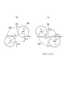
- FIGS. 13A and 13B are diagrams showing how the ball center changes due to the first rotation.
- FIG. 13A shows the position of the ball core before the first rotation
- FIG. 13B shows the ball center after the first rotation.
- (C) shows the amount of movement of the ball center by the first rotation.
- the test optical system 22 is composed of four lens surfaces.
- the ball center 70, the ball center 71, the ball center 72, and the ball center 73 are located on one side of the first rotation axis. ing.
- the ball center 70, the ball center 71, the ball center 72, and the ball center 73 move to the other side of the first rotation axis. .
- the other side is at a position opposite to the one side across the first rotation shaft.
- the eccentric amount of the sphere center with respect to the measurement axis is ⁇ 1 for the sphere center 70, ⁇ 2 for the sphere center 71, ⁇ 3 for the sphere center 72, and ⁇ 4 for the sphere center 73.
- Each of the spherical center 70, the spherical center 71, the spherical center 72, and the spherical center 73 is displaced by the rotation of the test optical system. This amount of displacement is -2 times the amount of eccentricity with respect to the measurement axis before rotation.
- a predetermined aberration component is extracted from the final wavefront data.
- the predetermined aberration component is an aberration amount corresponding to ⁇ 2 times the amount of eccentricity with respect to the measurement axis. In this way, even when system aberration exists, it is possible to extract an aberration amount that is -2 times the amount of eccentricity with respect to the measurement axis.
- step S300 is executed.
- step S300 the first aberration component is extracted.
- Step S400 is executed using the extracted first aberration component.
- the eccentric amounts ⁇ 1 to ⁇ j at this time are ⁇ 2 times the eccentric amount with respect to the measurement axis.
- the amount of eccentricity obtained in the execution of step S400 is divided by -2, the amount of eccentricity with respect to the measurement axis can be obtained. Note that the amount of decentering at this time is the amount of decentering before the test optical system rotates.
- the eccentricity measuring method of the present embodiment even when system aberration exists in the light projecting system and the light receiving system, regardless of the shape of the lens surface and the number of lenses constituting the optical system.
- the amount of eccentricity can be measured in a short time.
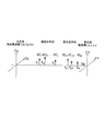
- the amount of eccentricity between the lens surfaces may be evaluated.
- a new axis 80 is set so that the amount of eccentricity of the plurality of lens surfaces distributed in the space is minimized. Then, the eccentric amount of the lens surface may be evaluated using the new axis 80 as a reference.
- the new axis 80 is set by, for example, setting a temporary axis and taking the sum of squares for all lens surfaces with respect to the distance from the temporary axis to the sphere. Then, the temporary axis may be changed so that the temporary axis when the sum of squares becomes the minimum becomes a new axis. Alternatively, the sum of squares is calculated for all lens surfaces with respect to the amount obtained by dividing the distance from the temporary axis to the sphere center by the radius of curvature of the lens. Then, the temporary axis may be changed, and the temporary axis when the sum of squares is minimized may be a new axis.
- the design aberration component can be removed even when the design aberration component exists.
- the wavefront aberration W in the equations (1-4), (1-5), and (1-6) has been described as a deviation from the wavefront when the test optical system is not decentered and has no system aberration.
- the wavefront aberration W is a deviation from an ideal wavefront such as a plane wave or a spherical wave
- the same explanation can be made by adding the term of the design aberration component M (Ox, Oy, ⁇ x, ⁇ y) to W.
- the designed aberration component M (Ox, Oy, ⁇ x, ⁇ y) is an aberration component that does not depend on the amount of decentering expressed only by the object height coordinate and the pupil coordinate. Therefore, it can be handled in the same manner as the system aberration component Sys (Ox, Oy, ⁇ x, ⁇ y).
- Sys (Ox, Oy, ⁇ x, ⁇ y) in equation (1-5) and Sys (Ox, Oy, ⁇ x, ⁇ y) in equation (1-6) are respectively represented by M (Ox, Oy, ⁇ x, ⁇ y).
- the design aberration component M (Ox, Oy, ⁇ x, ⁇ y) is the same in the equations (1-5) and (1-6). Therefore, when the calculation of equation (18) is performed in step S200, M (Ox, Oy, ⁇ x, ⁇ y) is removed. As a result, a predetermined aberration component can be extracted.
- the optical system under test has rotationally symmetric manufacturing errors such as a curvature radius error, a surface spacing error, and a refractive index error of each surface in addition to the decentration. Therefore, the wavefront aberration W actually measured includes an aberration component caused by a manufacturing error.
- the wavefront aberration component caused by the rotationally symmetric manufacturing error is also an aberration component that does not depend on the amount of decentering expressed only by the object height coordinate and the pupil coordinate. Therefore, it can be handled in the same manner as the system aberration component Sys (Ox, Oy, ⁇ x, ⁇ y) and the design aberration component M (Ox, Oy, ⁇ x, ⁇ y). Therefore, even if there is a rotationally symmetric manufacturing error such as a curvature radius error, a surface distance error, and a refractive index error in each surface in the test optical system, a predetermined aberration component can be extracted.
- the test optical system may analyze the deviation of the wavefront after the first rotation with respect to the wavefront before the first rotation.
- step S300 is executed.
- step S300 the first aberration component is extracted.
- Step S400 is executed using the extracted first aberration component.
- the decentering amount measuring method of the present embodiment even when there is a design aberration in the test optical system, it is short regardless of the shape of the lens surface and the number of lenses constituting the optical system.
- the amount of eccentricity can be measured over time.
- the aberration component of the light receiving optical system can be removed even when the light receiving optical system disposed between the test optical system and the light receiving system is decentered.
- FIG. 14 is a diagram illustrating a state in which the light receiving optical system is disposed between the test optical system and the light receiving system. Here, it is assumed that no system aberration or design aberration has occurred.
- the light receiving optical system includes lens surfaces from the (j + 1) th lens surface to the mth lens surface.
- the lens surface shift is represented using a spherical center.
- SC j + 1 , SC j + 2 ,..., SC m represent the sphere centers of the lens surfaces.
- ⁇ j + 1 , ⁇ j + 2 ,..., ⁇ m represent the shift amount in the Y direction of each lens surface.
- the wavefront aberration of the wavefront incident on the receiving system is the sum of the wavefront aberration generated by the decentering of the receiving optical system in addition to the wavefront aberration generated by the decentering of the test optical system. become. Therefore, the wavefront finally detected has the decentration aberration of the optical system to be detected and the decentration aberration of the light receiving optical system.
- wavefront data WFD ⁇ 1 is acquired by executing Step S110 and Step S121.
- the wavefront data WFD ⁇ 1 includes information on the decentration aberration of the optical system to be measured and information on the decentration aberration of the light receiving optical system.
- the wavefront aberration W is obtained by analyzing the wavefront data WFD ⁇ 1.
- the wavefront aberration W is expressed by the following equation (1-7).
- the eccentricity is a shift in the Y direction
- the amount of eccentricity is represented by ⁇ .
- W (Ox, Oy, ⁇ x, ⁇ y, ⁇ 1 , ⁇ 2 , ..., ⁇ j ) ⁇ 1 B 11 (Ox, Oy, ⁇ x, ⁇ y) + ⁇ 1 2 B 12 (Ox, Oy, ⁇ x, ⁇ y) + ⁇ 2 B 21 (Ox, Oy, ⁇ x, ⁇ y) + ⁇ 2 2 B 22 (Ox, Oy, ⁇ x, ⁇ y) + ...
- step S150 is executed.
- the first rotation is performed.
- the test optical system is rotated around the measurement axis.
- the rotation angle is, for example, 180 °. Note that the position of the light projecting system remains fixed. Therefore, the irradiation position P does not move. Further, the positions of the light receiving optical system and the light receiving system remain fixed.
- the wavefront data WFD ⁇ 2 is acquired by executing Step S110 and Step S122.
- the wavefront data WFD ⁇ 2 includes information on the decentration aberration of the optical system to be measured and information on the decentration aberration of the light receiving optical system.
- the wavefront aberration W is obtained by analyzing the wavefront data WFD ⁇ 2.
- the wavefront aberration W is expressed by the following equation (1-8).
- W (Ox, Oy, ⁇ x, ⁇ y, - ⁇ 1 , - ⁇ 2 , ..., - ⁇ j ) (- ⁇ 1 ) B 11 (Ox, Oy, ⁇ x, ⁇ y) + (- ⁇ 1 ) 2 B 12 (Ox, Oy, ⁇ x, ⁇ y) + (- ⁇ 2 ) B 21 (Ox, Oy, ⁇ x, ⁇ y) + (- ⁇ 2 ) 2 B 22 (Ox, Oy, ⁇ x, ⁇ y) + ...
- Table 15 shows the result of comparing the decentration aberration component of the light receiving optical system with the equations (1-7) and (1-8). As can be seen from Table 15, the decentration aberration component of the light receiving optical system is the same in the equations (1-7) and (1-8).
- step S200 the calculation of Expression (18) is performed. Since the decentration aberration component of the light receiving optical system is removed by this calculation, a predetermined aberration component can be extracted.
- step S300 is executed.
- step S300 the first aberration component is extracted.
- Step S400 is executed using the extracted first aberration component.
- the decentration amount measuring method of the present embodiment even in the case where there is a decentered light receiving optical system, the time is short regardless of the shape of the lens surface and the number of lenses constituting the optical system.
- the amount of eccentricity can be measured.
- step S100 in FIG. 8 may be performed at a plurality of irradiation positions.
- the wavefront of the light beam emitted from the test optical system is measured by the light receiving system, and the wavefront data is recorded.
- the first rotation is performed by a certain angle.
- the wavefront of the light beam emitted from the test optical system is measured by the light receiving system off-axis and on-axis, and the wavefront data is recorded.
- the irradiation position is on the measurement axis
- off-axis the case where the irradiation position is not on the measurement axis.
- the acquisition step includes a first rotation.
- the test optical system is rotated around an axis parallel to the measurement axis, and the first irradiation position is the same at the same irradiation position.
- Wavefront data before one rotation and wavefront data after the first rotation can be acquired.
- the first rotation is performed around the first rotation axis.
- the first rotation axis is an axis different from the measurement axis, and is an axis that rotates the optical system to be measured about the optical axis.
- FIG. 15 is a diagram illustrating a state where the first rotation axis is eccentric with respect to the measurement axis.
- the first rotation axis AX R1 is shifted in the Y direction with respect to the measurement axis, that is, the Oz axis.
- E be the shift amount at this time.
- step S110 is executed to irradiate the optical system to be examined from the irradiation position P (Ox, Oy, 0).
- step S121 is executed to acquire the wavefront data WFD ⁇ 1.
- the wavefront aberration W is expressed by the following equation (1-9).
- the eccentricity of the optical system to be detected is a shift in the Y direction, the amount of eccentricity is represented by ⁇ .
- the magnitudes of E and ⁇ can be suppressed to a very small amount.
- the amount of aberration in each term is considered to be very small and can be ignored. it can.
- (1-9) does not include a term proportional to the cube of the amount of eccentricity.
- W (Ox, Oy, ⁇ x, ⁇ y, ⁇ 1 + E, ⁇ 2 + E, ..., ⁇ j + E) ( ⁇ 1 + E) B 11 (Ox, Oy, ⁇ x, ⁇ y) + ( ⁇ 1 + E) 2 B 12 (Ox, Oy, ⁇ x, ⁇ y) + ( ⁇ 2 + E) B 21 (Ox, Oy, ⁇ x, ⁇ y) + ( ⁇ 2 + E) 2 B 22 (Ox, Oy, ⁇ x, ⁇ y) + ... + ( ⁇ j + E) B j1 (Ox, Oy, ⁇ x, ⁇ y) + ( ⁇ j + E) 2 B j2 (Ox, Oy, ⁇ x, ⁇ y) (1-9)
- step S150 is executed.
- the first rotation is performed.
- the test optical system 20 is rotated around the measurement axis.
- the rotation angle is, for example, 180 °.
- step S110 is executed to irradiate the optical system to be examined from the irradiation position P (Ox, Oy, 0). Then, step S122 is executed to obtain the wavefront data WFD ⁇ 2.
- the wavefront aberration W is expressed by the following equation (1-10).
- W (Ox, Oy, ⁇ x, ⁇ y, - ⁇ 1 + E, - ⁇ 2 + E, ..., - ⁇ j + E) (- ⁇ 1 + E) B 11 (Ox, Oy, ⁇ x, ⁇ y) + (- ⁇ 1 + E) 2 B 12 (Ox, Oy, ⁇ x, ⁇ y) + (- ⁇ 2 + E) B 21 (Ox, Oy, ⁇ x, ⁇ y) + (- ⁇ 2 + E) 2 B 22 (Ox, Oy, ⁇ x, ⁇ y) + ... + (- ⁇ j + E) B j1 (Ox, Oy, ⁇ x, ⁇ y) + (- ⁇ j + E) 2 B j2 (Ox, Oy, ⁇ x, ⁇ y) (1-10)
- Step S200 is executed.
- the wavefront data WFD ⁇ 1 acquired before the first rotation is reference data
- the wavefront data WFD ⁇ 2 acquired after the first rotation is measurement data. Therefore, the final wavefront aberration is obtained by analyzing the measurement data using the reference data as the wavefront standard.
- the wavefront aberration represented by the equation (1-9) is used as reference data, and the wavefront aberration represented by the equation (1-10) is used as measurement data.
- the calculation of Expression (19) is performed. W (Ox, Oy, ⁇ x, ⁇ y, - ⁇ 1 + E, - ⁇ 2 + E, ..., - ⁇ j + E) -W (Ox, Oy, ⁇ x, ⁇ y, ⁇ 1 + E, ⁇ 2 + E, ..., ⁇ j + E) (19)
- B j1 (Ox, Oy, ⁇ x, ⁇ y) + [(- ⁇ j + E) 2- ( ⁇ j + E) 2 ]
- B 12 (Ox, Oy, ⁇ x, ⁇ y) + (-2 ⁇ 2 )
- B 21 (Ox, Oy, ⁇ x, ⁇ y) + (-4 ⁇ 2 E)
- B 22 (Ox, Oy, ⁇ x, ⁇ y) + ... + (-2 ⁇ j ) B j1 (Ox, Oy, ⁇ x, ⁇ y) + (-4 ⁇ j E) B j2 (Ox, Oy, ⁇ x, ⁇ y) (1-11)
- the wavefront aberration expressed by Equation (1-11) is a deviation of the wavefront after the first rotation with respect to the wavefront before the first rotation of the optical system to be tested.
- the final wavefront aberration includes an aberration component proportional to the first power of the decentering amount and an aberration component proportional to the second power of the decentering amount, that is, the first aberration component and the second aberration component.
- Aberration components are extracted by performing the calculation of Expression (19).
- the formula (1-9) and the formula (1-10) do not include the design aberration component, the system aberration component, and the decentration aberration component of the light receiving optical system. However, these aberration components may be included. However, these aberration components are removed by performing the calculation of equation (19). For these reasons, these aberration components are not described in the equations (1-9) and (1-10).
- Equation (1-11) includes the second aberration component. This is because the first rotation axis is shifted by the shift amount E with respect to the measurement axis. Therefore, the amount of eccentricity cannot be obtained using the equation regarding the first eccentric component as it is.
- the wavefront data before the first rotation and the wavefront data after the first rotation are acquired at the irradiation position P ′.
- Wavefront data before the first rotation is reference data
- wavefront data after the first rotation is measurement data. Therefore, the final wavefront aberration at the irradiation position P ′ is obtained by analyzing the measurement data using the reference data as the wavefront standard.
- the wavefront aberration expressed by Equation (1-12) is the deviation of the wavefront after the first rotation with respect to the wavefront before the first rotation of the optical system under test.
- the final wavefront aberration is proportional to the aberration component proportional to the first power of the decentering amount and the square of the decentering amount as the predetermined aberration component. It has an aberration component, that is, a first aberration component and a second aberration component.
- step S300 is executed to extract the first aberration component.
- the aberration component is represented by Wz.
- the aberration component Wz multiplied by the odd-order function of the pupil coordinates is an aberration component multiplied by the second term of the Zernike term.
- Wz 2 3, 7, 8,.
- the sum of Expression (1-11) and Expression (1-12) is taken. The result is shown in equation (20).
- the first aberration component Tz (Ox, Oy, ⁇ 1, ⁇ 2, ..., ⁇ j ) can be extracted from the predetermined aberration component.
- the aberration component Wz multiplied by the even-order function of the pupil coordinates is an aberration component multiplied by the fourth term of the Zernike term.
- the first aberration component Tz (Ox, Oy, ⁇ 1, ⁇ 2, ..., ⁇ j ) can be extracted from the predetermined aberration component.
- the coefficient is in the ⁇ 1, ⁇ 2, ⁇ , ⁇ j.
- ⁇ 1 , ⁇ 2 ,..., ⁇ j are eccentric amounts from the first rotation axis.
- the reference representing the amount of eccentricity is the first rotation axis. That is, the measurement axis is not a standard for representing the amount of eccentricity.
- Step S400 is executed using the first aberration component Tz (Ox, Oy, ⁇ 1, ⁇ 2, ..., ⁇ j ).
- step S400 simultaneous linear equations are solved. As a result, a value that is ⁇ 2 times the amount of eccentricity with respect to the first rotation axis is obtained as a solution.
- the second aberration component disappears and the first aberration component is extracted, so that the displacement of each surface of the optical system to be measured and the aberration amount of the first aberration component can be handled linearly.
- the displacement amount of each surface accompanying the rotation around the first rotation axis AX R1 of the optical system to be measured can be obtained. Therefore, the amount of eccentricity can be accurately obtained with reference to the first rotation axis.
- two wavefront data are acquired by rotating the optical system to be measured at a certain angle around the measurement axis or the first rotation axis.
- the angle at which the optical system to be tested is rotated is 10 degrees or more. Furthermore, it is preferable that the angle at which the test optical system is rotated is 180 degrees.
- the test optical system is rotated 180 degrees around the measurement axis or the first rotation axis.
- the rotation angle may be any number.
- a preferable rotation angle is 10 degrees or more, and a more preferable angle is 180 degrees.
- the first rotation axis may tilt with respect to the measurement axis. This point will be described.
- FIG. 16 is a diagram showing a relative relationship between the first rotation axis and the measurement axis, where (a) shows a state in which the measurement axis and the first rotation axis coincide with each other, and (b) shows the measurement axis relative to the measurement axis.
- the first rotating shaft is tilted.
- the lens surface of the test optical system 90 is an aspherical surface
- the state of displacement by the first rotation is as shown in FIG.
- the aspheric surface 91 is represented by an aspheric surface apex 92 and an aspheric surface axis 93.
- the displacement amount of the aspheric surface top and the displacement amount of the aspheric axis are ⁇ 2 times the eccentricity with respect to the first rotation axis AX R1 before the rotation.
- the aspheric surface apex 92 is displaced to the position of the aspheric surface apex 92 ′ by the first rotation.
- the displacement amount of the aspheric surface top 92 is ⁇ 2 ⁇ y1.
- the displacement amount of the aspherical axis 93 is ⁇ 2 ⁇ a1.
- the displacement amount of each surface associated with the rotation of the optical system to be tested around the first rotation axis can be obtained from the first aberration component. Based on this amount of displacement, the amount of eccentricity based on the first rotation axis of the optical system to be tested can be obtained. Therefore, the displacement amount of each surface accompanying the rotation of the test optical system around the first rotation axis needs to reflect the amount of eccentricity of the test optical system.
- the first rotation axis AX R1 When performing the first rotation, it is desirable that the first rotation axis AX R1 coincides with the measurement axis AX M. However, a shift or tilt may occur on the first rotation axis AX R1 with respect to the measurement axis AX M. In this case, there is no practical problem if the shift amount and tilt amount are small. In particular, when the first rotation axis AX R1 is shifted with respect to the measurement axis AX M , the displacement amount associated with the first rotation is not affected. Therefore, in this case, the displacement amount of each surface accurately reflects the eccentric amount of each surface.
- the tilt affects the amount of displacement associated with the first rotation.
- the first rotation axis AX R1 is tilted at an angle ⁇ with respect to the measurement axis AX M.
- the decentration amount of the test optical system can be obtained without any problem.
- FIG. 17 is a diagram illustrating a state in which the first rotation axis is blurred with respect to the measurement axis.
- the blur generated on the first rotation axis AX R1 can be represented by a shift and a tilt with respect to the measurement axis AX M.
- the first rotation axis AX R1 is shifted by the distance T with respect to the measurement axis AX M and tilted by the angle ⁇ .
- the amount of displacement of the aspheric surface top 92 reflects the amount of eccentricity almost accurately.
- an extra displacement 95 occurs at the aspheric surface top other than the aspheric surface top 92.
- the displacement 95 at the aspheric surface apex 94 is d4 sin ⁇ . Therefore, the amount of displacement at the aspheric surface apex 94 is ⁇ y4 + T ⁇ y4 ⁇ cos ⁇ + d4 sin ⁇ .
- d4 is the distance of the measuring axis AX M direction of the aspheric surface apex 92 aspheric surface apex 94. That is, the displacement is added by sin ⁇ times the distance in the measurement axis AX M direction.
- the virtual rotation axis AX I is an axis shifted by a distance T / 2 with respect to the measurement axis AX M and tilted by an angle ⁇ / 2. It can be considered that the test optical system rotates around this virtual rotation axis AX I. Therefore, the displacement amount of each surface associated with the rotation around the virtual rotation axis AX I can be obtained from the first aberration component. Based on this amount of displacement, the amount of eccentricity based on the virtual rotation axis AX I of the test optical system can be obtained. Therefore, even if the first rotation axis is tilted with respect to the measurement axis, there is no practical problem.
- the first rotation can be performed even when the light beam is irradiated from a set of irradiation positions.
- An execution example of the first rotation will be described using execution example 1 and execution example 2.
- FIG. 18 shows a flowchart of the execution example 1.
- the first rotation is performed at one irradiation position, and the wavefront data before the first rotation and the wavefront data after the first rotation are acquired.
- the irradiation position is changed, the first rotation is performed at the other irradiation position, and wavefront data before the first rotation and wavefront data after the first rotation are acquired.
- Step S100 includes Step S110, Step S121, Step S122, Step S130, Step S141, Step S142, Step S150, and Step S151.
- step S100 step S110, step S121, step S150, step S110 and step S122 are executed.
- step S110, step S121, step S150, step S110 and step S122 are executed.
- the wavefront data WFD ⁇ 1 before the first rotation and the wavefront data WFD ⁇ 2 after the first rotation are acquired at the irradiation position P.
- step S151 is executed to return the test optical system to the state before the first rotation.
- Step S130, Step S141, Step S150, Step S130 and Step S142 are executed. Thereby, at the irradiation position P ′, the wavefront data WFD′ ⁇ 1 before the first rotation and the wavefront data WFD′ ⁇ 2 after the first rotation are acquired.
- the light source is driven in the OxOy direction, the light source is positioned at an arbitrary OxOy coordinate, and reference data is acquired. That is, reference data is acquired at an arbitrary object height coordinate (Ox, Oy). Thereafter, the first rotation is performed to rotate the test optical system.
- the measurement data is acquired after the first rotation.
- the coordinates of the light source that is, the object height coordinates (Ox, Oy) are not changed before the first rotation and after the first rotation. Therefore, measurement data is acquired at the same object height coordinates (Ox, Oy) as before the first rotation.
- the light source is driven in the OxOy direction, the light source is positioned at a coordinate different from the first OxOy coordinate, and reference data is acquired. That is, the reference data is acquired at object height coordinates (Ox ′, Oy ′) different from the first object height coordinates (Ox, Oy). Thereafter, the first rotation is performed to acquire measurement data.
- the acquisition of the reference data and the acquisition of the measurement data are alternately repeated. Then, after completing the acquisition of reference data and the acquisition of measurement data at all object height coordinates, wavefront analysis is performed.
- step S130 and step S142 may be executed without executing step S151 to acquire the wavefront data WFD' ⁇ 2. Thereafter, step S151 is executed to return the test optical system to the state before the first rotation. Then, step S130 and step S141 may be executed to acquire the wavefront data WFD' ⁇ 1.
- the wavefront data before the first rotation and the wavefront data after the first rotation can be acquired at each irradiation position.
- the design aberration, the system aberration, and the decentration aberration of the light receiving optical system can be removed. .
- FIG. 19 is a diagram showing a flowchart of the execution example 2.
- the execution example 2 first, wavefront data is acquired at one irradiation position and the other irradiation position. Thereafter, the first rotation is performed, and wavefront data is acquired again at one irradiation position and the other irradiation position.
- Step S100 includes Step S110, Step S121, Step S122, Step S130, Step S141, Step S142, and Step S150.
- step S100 first, step S110, step S121, step S130, and step S141 are executed. Thereby, the wavefront data WFD ⁇ 1 at the irradiation position P and the wavefront data WFD′ ⁇ 1 at the irradiation position P ′ are acquired in the state before the first rotation.
- Step S150 is executed to rotate the optical system to be examined. Subsequently, step S110, step S122, step S130, and step S142 are executed. Thereby, the wavefront data WFD ⁇ 2 at the irradiation position P and the wavefront data WFD′ ⁇ 2 at the irradiation position P ′ are acquired in the state after the first rotation.
- the light source before the first rotation, the light source is driven in the OxOy direction, the light source is positioned at a plurality of object height coordinates, and reference data is acquired. That is, all the acquisition of the reference data is completed at a plurality of object height coordinates. Thereafter, the first rotation is performed to rotate the test optical system.
- the light source After the first rotation, drive the light source again in the OxOy direction to acquire measurement data.
- the light source In acquiring the measurement data, the light source is positioned at the same OxOy coordinates as before the first rotation. That is, all acquisition of measurement data is completed at the same object height coordinates as before the first rotation. Then, after all the measurement data acquisition is completed, the wavefront analysis is performed.
- the first rotation is executed.
- the aberration component proportional to the first power of the decentering amount among the decentering aberrations accompanying the decentering of the optical system under test that is, the first An aberration component can be extracted.
- step S142 may be executed to acquire the wavefront data WFD' ⁇ 2.
- step S110 and step S122 may be executed to obtain the wavefront data WFD ⁇ 2.
- the wavefront data before the first rotation and the wavefront data after the first rotation can be acquired at each irradiation position.
- the design aberration, the system aberration, and the decentration aberration of the light receiving optical system can be removed. .
- the measurement method of the present embodiment it is preferable to move one irradiation position and the other irradiation position, respectively, and acquire wavefront data at the moved irradiation position.
- ⁇ One lens has two lens surfaces.
- the number of degrees of freedom in eccentricity is 8 when a shift and tilt occur on each lens surface.
- the number of degrees of freedom in decentration is 16 when shift and tilt occur on each lens surface.
- An increase in the number of eccentric degrees of freedom means that the number of j increases in ⁇ 1 to ⁇ j in equations (9-1) to (9-9).
- ⁇ 1 to ⁇ j are unknown numbers, if the number of linear equations is 9 at the maximum, ⁇ 9 can be obtained, but ⁇ 10 or more cannot be obtained.
- the number of linear equations can be increased by increasing the irradiation position. Therefore, according to the measurement method of this embodiment, the measurable degree of freedom of eccentricity can be increased.
- one irradiation position is moved, all wavefront data is acquired at the irradiation position after movement, the other irradiation position is then moved, and the wavefront data is moved at the irradiation position after movement. It is preferable to acquire all.
- FIG. 20 shows a flowchart of the measurement method of this embodiment.
- step S200 and subsequent steps are omitted.
- FIG. 21 is a diagram showing the movement of the irradiation position, in which (a) shows the position before movement of one irradiation position, (b) shows the position after movement of one irradiation position, (C) shows the position before movement of the other irradiation position, and (d) shows the position after movement of the other irradiation position.
- Step S100 includes Step S111, Step S123, Step S131, Step S143, Step S160, Step S161, Step S170, and Step S171.
- step S100 a light beam is irradiated from the irradiation position Pn and the irradiation position P'n.
- the irradiation position Pn is one irradiation position
- the irradiation position P′n is the other irradiation position.
- the irradiation position Pn and the irradiation position P′n are symmetric with respect to the measurement axis.
- the number N of times of changing the irradiation position is set by the user.
- the number N is the scheduled number.
- the value of n is set to 0.
- n represents the number of movements of the irradiation position.
- step S111 is executed.
- the light beam is irradiated from the irradiation position Pn.
- the light source is positioned at the irradiation position P0 (Ox0, Oy0, 0). Since target optical system 2 is eccentric relative to the measuring axis, the non-plane wave 9 0 is emitted from the optical system 2. Non plane wave 9 0 is detected by the light receiving system 3.
- step S123 is executed.
- the wavefront data WFDn is obtained based on the non-plane wave 9 0.
- step S160 is executed.
- step S160 n and N are compared. When n and N are not equal, the number of movements of the irradiation position has not reached the scheduled number. Therefore, 1 is added to the current number of movements, and step S170 is executed. In step S170, the irradiation position is moved. The movement amount may be set in advance by the user.
- step S111 is executed again. At this time, since the irradiation position is moved, the light source is positioned at the irradiation position P1 (Ox1, Oy1,0) as shown in FIG. Non plane wave 9 1 from the optical system 2 is emitted. Non plane wave 9 1 is detected by the light receiving system 3.
- non-plane wave 9 1 is different from the non-plane wave 9 0.
- step S123 is executed.
- the wavefront data WFDn is obtained based on the non-plane wave 9 1.
- the movement of the irradiation position and the acquisition of the wavefront data WFDn are performed until n and N are equal. All the acquired wavefront data WFDn is stored.
- step S160 If n and N are equal in step S160, the movement of the irradiation position is completed. In this way, the movement of one irradiation position and the acquisition of wavefront data at the irradiation position after the movement are completed. Then, the value of n is set to 0.
- step S131 is executed.
- the light beam is irradiated from the irradiation position P′n.
- the light source is positioned at the irradiation position P′0 ( ⁇ Ox0, ⁇ Oy0,0).
- the irradiation position P′0 ( ⁇ Ox0, ⁇ Oy0,0) is a position symmetrical to the irradiation position P0 (Ox0, Oy0,0) with respect to the measurement axis.
- Non plane wave 9 '0 from the optical system 2 is emitted.
- the non-planar wave 9 ′ 0 is detected by the light receiving system 3.
- non-plane wave 9 '0 is different from the non-plane wave 9 0 and a non-plane wave 9 1.
- step S143 is executed.
- step S143 the wavefront data WFD'n is obtained based on the non-plane wave 9 '0. Thereafter, step S161 is executed.
- step S161 n and N are compared. When n and N are not equal, the number of movements of the irradiation position has not reached the scheduled number. Therefore, 1 is added to the current number of movements, and step S171 is executed. In step S171, the irradiation position is moved. The movement amount may be set in advance by the user.
- step S131 is executed again.
- the light source is positioned at the irradiation position P′1 ( ⁇ Ox1, ⁇ Oy1,0) as shown in FIG.
- the irradiation position P′1 ( ⁇ Ox1, ⁇ Oy1,0) is a position symmetrical to the irradiation position P1 (Ox1, Oy1,0) with respect to the measurement axis.
- Non plane wave 9 '1 from the optical system 2 is emitted.
- the non-planar wave 9 ′ 1 is detected by the light receiving system 3.
- P′1 ( ⁇ Ox1, ⁇ Oy1,0) is an irradiation position P′0 ( ⁇ Ox0, ⁇ Oy0,0), P0 (Ox0, Oy0,0) and an irradiation position P1 (Ox1, Oy1,0). ) Is different. Therefore, non-plane wave 9 '1, non-plane wave 9' 0, a non-plane wave 9 0 and a non-plane wave 9 1 differs.
- step S143 is executed.
- the wavefront data WFD'n is obtained based on the non-plane wave 9 '1.
- the movement of the irradiation position and the acquisition of the wavefront data WFD′n are performed until n and N are equal. All the acquired wavefront data WFD′n is stored.
- step S161 when n and N become equal, the movement of the irradiation position ends. In this way, the movement of the other irradiation position and the acquisition of the wavefront data at the irradiation position after the movement are completed.
- the irradiation position P'0 (-Ox0, -Oy0,0) is moved. However, it may be moved to the irradiation position P'1 (-Ox1, -Oy1,0) and then moved to the irradiation position P'0 (-Ox0, -Oy0,0).
- the number of linear equations can be increased by increasing the irradiation position. Therefore, according to the measurement method of this embodiment, the measurable degree of freedom of eccentricity can be increased.
- the wavefront data is acquired at each of the one irradiation position and the other irradiation position, and then the one irradiation position and the other irradiation position are moved, and each of the irradiation positions after the movement is moved. It is preferable to acquire wavefront data at
- FIG. 22 shows a flowchart of the measurement method of the present embodiment. Note that step S200 and subsequent steps are omitted.
- FIG. 23 is a diagram showing the movement of the irradiation position, where (a) shows the position before movement of one irradiation position, (b) shows the position of the other irradiation position before movement, (C) shows the position after movement of one irradiation position, and (d) shows the position after movement of the other irradiation position.
- step S100 includes step S111, step S123, step S131, step S143, step S162, and step S172.
- step S111 is executed.
- the light beam is irradiated from the irradiation position Pn.
- the light source is located at the irradiation position P0 (Ox0, Oy0, 0).
- step S123 is executed.
- the wavefront data WFDn is obtained based on the non-plane wave 9 0.
- step S131 is executed.
- the light beam is irradiated from the irradiation position P'n.
- the light source is positioned at the irradiation position P′0 ( ⁇ Ox0, ⁇ Oy0,0).
- step S143 is executed.
- step S143 the wavefront data WFD'n is obtained based on the non-plane wave 9 '0. Thereafter, step S162 is executed.
- step S162 n and N are compared. When n and N are not equal, the number of movements of the irradiation position has not reached the scheduled number. Therefore, 1 is added to the current number of movements, and step S172 is executed. In step S172, the irradiation position is moved. The movement amount may be set in advance by the user.
- step S111 is executed again. At this time, since the irradiation position is moved, the light source is positioned at the irradiation position P1 (Ox1, Oy1,0) as shown in FIG.
- step S123 is executed.
- the wavefront data WFDn is obtained based on the non-plane wave 9 1.
- step S131 is executed.
- the light beam is irradiated from the irradiation position P'n.
- the light source is positioned at the irradiation position P′1 ( ⁇ Ox1, ⁇ Oy1,0) as shown in FIG.
- step S143 is executed.
- step S143 the wavefront data WFD'n is obtained based on the non-plane wave 9 '1. Thereafter, step S162 is executed.
- the movement of the irradiation position and the acquisition of the wavefront data WFDn and the wavefront data WFD'n are performed until n and N are equal.
- the acquired wavefront data WFDn and wavefront data WFD'n are all stored.
- step S162 If n and N are equal in step S162, the movement of the irradiation position is completed. In this way, the movement of one irradiation position and the other irradiation position and the acquisition of wavefront data at the irradiation position after the movement are completed.
- the number of linear equations can be increased by increasing the irradiation position. Therefore, according to the measurement method of this embodiment, the measurable degree of freedom of eccentricity can be increased.
- the moving direction of the irradiation position is a direction approaching the Oz axis.
- the direction of movement of the irradiation position may be a direction away from the Oz axis.
- 21 and 23 show four irradiation positions, the irradiation positions are not limited to four.
- the light beam may be irradiated from the origin (0,0,0).
- FIGS. 24A and 24B are diagrams showing how the irradiation position moves.
- FIG. 24A shows a case where the movement direction of the irradiation position is one direction
- FIG. 24B shows a case where the movement direction of the irradiation position is two directions. Yes.
- FIG. 24A The movement in one direction of the irradiation position is shown in FIG. In FIG. 24A, the movement of the irradiation position is started from the negative maximum object height coordinate. Then, the irradiation position moves toward the positive maximum object height coordinate. That is, the irradiation position moves in the order of the irradiation position P′4 ( ⁇ Ox4,0,0), the irradiation position P0 (0,0,0), and the irradiation position P4 (Ox4,0,0).
- FIG.23 (b) The movement of the irradiation position in two directions is shown in FIG. In FIG.23 (b), the movement of the irradiation position is started from the axis. Then, the irradiation position moves toward the positive maximum object height. Next, the irradiation position is returned to the axis (on the Oz axis), and the irradiation position moves toward the negative maximum object height. That is, the irradiation position moves from the irradiation position P0 (0,0,0) toward the irradiation position P4 (Ox4,0,0), and then the irradiation position P ′ from the irradiation position P0 (0,0,0). The irradiation position moves toward 4 (-Ox4, 0, 0).
- the irradiation position may be randomly moved from the irradiation position P4 (Ox4,0,0) to the irradiation position P4 ′ ( ⁇ Ox4,0,0).
- the irradiation position may be moved randomly between '4 (-Ox4, 0, 0).
- the number of linear equations can be increased by increasing the irradiation position. Therefore, the measurable degree of eccentricity can be increased.
- FIG. 25A and 25B are diagrams showing irradiation position patterns, where FIG. 25A shows a state in which the irradiation position is in two directions, FIG. 25B shows a state in which the irradiation position is concentric, and FIG. The state is shown.
- the irradiation position in the light projecting system 1 is located only on the Ox axis and the Oy axis.
- the irradiation position in the light projecting system 1 is also located between the Ox axis and the Oy axis.
- the irradiation position is located concentrically or radially.
- the irradiation position is located in the grid
- the standard of the pitch of movement of the irradiation position in the light projecting system 1 may be about 1/50 of the effective aperture from about the effective aperture of the optical system to be tested.
- the movement pitch is made smaller and more wavefront data is acquired.
- the diameter of the irradiated light beam may be approximately the same as the diameter of the test optical system.
- the object height is made small so that the light beam is not scattered outside the effective aperture of the optical system to be tested.
- the number of linear equations can be increased by increasing the irradiation position. Therefore, the measurable degree of eccentricity can be increased.
- the wavefront data is acquired in the first irradiation state, and that the central ray of the light beam is parallel to the measurement axis in the first irradiation state.
- the central ray of the light beam is parallel to the measurement axis. That is, as shown in FIG. 6, the central ray CR of the light beam emitted from the irradiation position P (Ox, Oy, 0) of the light projecting system 1 is parallel to the Oz axis, that is, the measurement axis.
- the irradiation position P (Ox, Oy, 0) is changed in the OxOy plane, the light beam emitted from the test optical system 2 changes.
- the incident angle of the light flux to the light receiving system 3 changes, but the incident position hardly changes. Therefore, the position adjustment between the light receiving system 3 and the light beam incident on the light receiving system 3 can be reduced.
- the wavefront data is acquired in the second irradiation state, and in the second irradiation state, the central ray of the light beam intersects with the measurement axis at a predetermined angle.
- FIGS. 26A and 26B are diagrams showing a state in which a test optical system is irradiated with a light beam.
- FIG. 26A shows irradiation at an angle ⁇
- FIG. 26B shows irradiation at an angle ⁇ ′.
- the central ray CR of the light beam emitted from the irradiation position P (Ox, Oy, 0) of the light projecting system 1 intersects the Oz axis, that is, the measurement axis at an angle ⁇ .
- the spherical wave 4 is emitted from the irradiation position P (Ox, Oy, 0).
- the test optical system 2 is irradiated with a light beam at a position and an angle different from those in FIG. Therefore, the non-plane waves 8 and 8 ′ emitted from the test optical system 2 are different from the non-plane waves 7 and 7 ′ in FIG. 6.
- the second extraction step is performed using a predetermined function system
- the predetermined function system is a function system indicating the first aberration component, and one irradiation position. It is preferable to apply the predetermined aberration component at and the predetermined aberration component at the other irradiation position to a predetermined function system. In this way, an amount proportional to the first power of the amount of eccentricity ⁇ , that is, the first aberration component can be extracted.
- the acquisition step includes a second rotation.
- the test optical system is rotated 180 degrees around an axis orthogonal to the measurement axis, and the second rotation is performed. It is preferable to acquire the wavefront data and the wavefront data after the second rotation.
- FIG. 27 shows a flowchart of the measurement method of this embodiment.
- step S100 includes step S110, step S123, step S124, and step S180.
- Detailed descriptions of step S200, step S300, and step S400 are omitted.
- FIG. 28 is a diagram showing the second rotation, where (a) shows a state before the second rotation, and (b) shows a state after the second rotation.
- the test optical system 20 will be referred to as “front” and “rear”.
- the test optical system 20 when the test optical system 20 is irradiated with a light beam, the light beam can be irradiated from the lens 23 side or the light beam can be irradiated from the lens 25 side.
- the case where the light beam is irradiated from the lens 23 side is “front”
- the case where the light beam is irradiated from the lens 25 side is “back”.
- front measurement When the light beam is irradiated from the “front” to the test optical system 20 (hereinafter referred to as “front measurement”), and when the light beam is irradiated from the “back” to the test optical system 20 (hereinafter referred to as “rear measurement”).
- front measurement When the light beam is irradiated from the “front” to the test optical system 20 (hereinafter referred to as “front measurement”), and when the light beam is irradiated from the “back” to the test optical system 20 (hereinafter referred to as “rear measurement”).
- front measurement When the light beam is irradiated from the “front” to the test optical system 20 (hereinafter referred to as “front measurement”), and when the light beam is irradiated from the “back” to the test optical system 20 (hereinafter referred to as “rear measurement”).
- rear measurement When the light beam is irradiated from the “back” to the test optical system 20 (hereinafter referred to as “rear measurement
- the test optical system 20 is composed of six lens surfaces, the first surface, the second surface,.
- the first surface through which the light beam is transmitted is the first surface.
- the light beam passes through the sixth surface, the fifth surface,... In this order, and the first surface is the last surface to be transmitted.
- the object point is relayed on each lens surface of the test optical system 20. Therefore, if a certain lens surface is decentered, the object point relayed to the rear side of the lens surface is shifted laterally from the ideal position. Then, it can be considered that this causes aberrations on the subsequent lens surfaces. In other words, the aberration caused by decentration is related to the order of the lens surfaces. This is the reason why the decentration aberration sensitivity changes depending on whether the test optical system 20 is measured on the front side or the rear side. In the measurement method of the present embodiment, the amount of information related to the first aberration component is increased by utilizing this fact.
- step S110 as shown in FIG. 28 (a), the optical system 20 is irradiated with a light beam from the irradiation position P (Ox, Oy, 0).
- the test optical system 20 is arranged so that the light projecting system 10 and the lens 23 face each other. Therefore, the light beam is irradiated onto the optical system 20 to be tested from the lens 23 side.
- a non-planar wave 51 is emitted from the test optical system 20. The non-planar wave 51 enters the light receiving system 30.
- step S123 is executed. Thereby, wavefront data WFD ⁇ 3 is acquired.
- step S180 is executed.
- the second rotation is performed.
- the test optical system 20 is rotated around an axis orthogonal to the measurement axis.
- the rotation angle is 180 °.
- the test optical system 20 is arranged so that the light projecting system 10 and the lens 25 face each other. Therefore, the optical system 20 is irradiated with the light beam from the lens 25 side.
- the positions of the light projecting system 10 and the light receiving system 30 do not move.
- step S110 is executed.
- step S110 as shown in FIG. 28 (b), the optical system 20 is irradiated with a light beam from the irradiation position P (Ox, Oy, 0).
- the wavefront 60 is incident on the test optical system 20.
- a non-planar wave 55 is emitted from the test optical system 20.
- the non-plane wave 56 is different from the non-plane wave 51.
- step S124 is executed. Thereby, wavefront data WFD ⁇ 4 is acquired.
- the wavefront data WFD ⁇ 3 and the wavefront data WFD ⁇ 4 are different. Therefore, finally, two first aberration components can be obtained.
- the number of first aberration components can be increased. Therefore, the measurable degree of eccentricity can be increased.
- FIGS. 29A and 29B are diagrams for explaining the change of the coordinate axes due to the second rotation, in which FIG. 29A shows a state before the second rotation, and FIG. 29B shows the state after the second rotation. Indicates the state.
- the test optical system is rotated by 180 ° around the Oy axis.
- the front side measurement is performed.
- the lens L1 is arranged on the origin (0, 0, 0) side
- the lens L2 is arranged after the lens L1. Therefore, the lens surfaces are the lens surface L1 1 , the lens surface L1 2 , the lens surface L2 1 , and the lens surface L2 2 in order from the origin (0, 0, 0) side.
- the coordinate axis XL2 and the Ox axis are in the same direction.
- the light beam is irradiated from the irradiation position P (Ox, Oy, 0) to the optical system under test.
- the light beam is irradiated in the order of the lens L1 and the lens L2.
- the lens L2 is disposed on the origin (0, 0, 0) side, and the lens L1 is disposed subsequent to the lens L2. Therefore, the lens surfaces are the lens surface L2 2 , the lens surface L2 1 , the lens surface L2 2 , and the lens surface L2 1 in order from the origin (0, 0, 0) side.
- coordinate axes X L2 has become Ox axis and opposite direction.
- the direction of the coordinate axis Y L2 is not changed, but the direction of the coordinate axis X L2 is reversed.
- the sphere center of the lens L2 is positioned on the plus side.
- the rear side measurement when the reference coordinate axes X L2, spherical center lens L5 are located on the positive side.
- the center of the lens L2 is positioned on the minus side in the rear measurement.
- the direction of the coordinate axis X L2 does not change, but the direction of the coordinate axis Y L2 differs by 180 °. Therefore, when the Oy axis is used as a reference, for example, if the sign of the ball center position in the front measurement is positive, the sign of the ball center position in the rear measurement is negative.
- the amount of eccentricity when acquiring the wavefront data before the second rotation and the amount of eccentricity when acquiring the wavefront data after the second rotation have the same absolute value. Preferably there is.
- the test optical system is rotated around the measurement axis. By doing in this way, the displacement amount which arises with this rotation can be calculated
- the same measurement system as that by the first rotation is used.
- the test optical system is arranged so that the front and back of the test optical system are reversed. Then, the first aberration component is extracted by performing the same processing as the measurement in the first rotation.
- the absolute value of the distance between the lens and the rotation axis needs to be the same between the front side measurement and the rear side measurement.
- the test optical system has six lens surfaces.
- all of the six lens surfaces are spherical.
- the eccentric amounts of the first surface, the second surface,..., The sixth surface during the front side measurement are (X1, Y1), (X2, Y2), (X6, Y6).
- the decentering amount of each lens surface is expressed by XY coordinates based on the first rotation axis.
- the test optical system When measuring the rear side, rotate the optical system to be tested for the front side measurement around the Y axis. As a result, the direction of the test optical system is reversed. Then, the rear side measurement is performed. At this time, the decentering amount of each lens surface in the rear side measurement is ( ⁇ X1, Y1), ( ⁇ X2, Y2)... ( ⁇ X6, Y6). Thus, the test optical system is arranged.
- the predetermined distance is a distance between the spherical center of each lens surface of the optical system to be measured and the first rotation axis at the time of front side measurement.
- first rotation may also be performed in the measurement method of the present embodiment.
- a plurality of wavefront data is acquired before and after the first rotation in the front side measurement.
- the second rotation is performed so that the rear side measurement is possible.
- the front and back of the test optical system are reversed.
- FIG. 30 is a diagram illustrating the movement of the ball center by the first rotation, in which (a) shows the movement of the ball center during the front side measurement, and (b) shows the movement of the ball center during the rear side measurement. Show.
- the lens surface in the vicinity of the spherical center is indicated by a circle. Thus, each of the two circles only displays a part of the same lens surface.
- the movement of the ball center at the time of front measurement will be described with reference to FIG.
- the ball center 96 Prior to the first rotation, the ball center 96 is located in the first quadrant of the OxOy coordinate system. Then, after the first rotation, the ball center 96 is located in the third quadrant.
- the movement amount of the ball center 96 is ⁇ f
- the x component is ⁇ X
- the y component is ⁇ Y.
- the movement of the ball center during back side measurement will be described with reference to FIG. Before the first rotation, the ball center 96 is located in the second quadrant of the OxOy coordinate system. Then, after the first rotation, the ball center 96 is located in the fourth quadrant.
- the movement amount of the ball center 96 is ⁇ r, the x component is ⁇ X, and the y component is ⁇ Y.
- the test optical system is arranged so that the absolute value of the predetermined distance is the same between the back side measurement and the front side measurement. Therefore,
- the direction of the Y component vector is the same between the front side measurement and the rear side measurement.
- the direction of the X component vector is reversed between the front side measurement and the back side measurement.
- FIG. 31 is a diagram showing the movement of the ball center due to the first rotation and the second rotation, where (a) shows the position of the ball center before the first rotation at the time of front measurement, and (b) At the time of the front side measurement, the position of the ball center after the first rotation is shown, (c) at the time of the rear side measurement, the position of the ball center before the first rotation, and (d) at the time of the rear side measurement. The position of the ball center after the first rotation is shown.
- the origin of the OxOy coordinates is the position of the first rotation axis. That is, FIG. 31 shows the position of the ball center with respect to the first rotation axis.
- the movement of the surface due to the first rotation and the second rotation of the aspheric surface is as follows. It can be indicated by the position of the surface top and the position of the aspherical axis.
- the Ox axis indicates the tilt amount in the B direction
- the Oy axis indicates the tilt amount in the A direction.
- the ball center 96 is located in the first quadrant of the OxOy coordinate system.
- the state after the first rotation is obtained at the time of the front side measurement.
- the ball center 96 is located in the third quadrant of the OxOy coordinate system.
- the absolute value of the displacement amount of the ball core 96 due to the first rotation is the same in FIG. 31 (b) and FIG. 31 (d). Moreover, it can also be seen from FIGS. 31B and 31D that the X direction of the movement vector of the ball center is opposite between the front side measurement and the back side measurement.
- the solution of the simultaneous linear equations for the eccentricity is the same in the front measurement and the rear measurement. Accordingly, simultaneous linear equations for the eccentricity can be solved by simultaneously using the eccentric aberration sensitivity proportional to the first power of the eccentricity of the front side measurement and the decentration aberration sensitivity proportional to the first power of the eccentricity of the rear side measurement. . In other words, the amount of decentration with many degrees of freedom can be obtained with high accuracy by using more cues for decentration aberration sensitivity.
- the obtained eccentricity is the position of the ball center in the state of FIG.
- the signs of the decentering aberration sensitivity of the aspherical surface are solved by reversing the signs of the decentering aberration sensitivity of the X-direction shift and the A-direction tilt. That's fine.
- the obtained tilt amount in the A direction is the aspherical axis tilt amount based on the first rotation axis before the first rotation at the time of the front side measurement.
- the second rotation is performed when the measurement in the front side measurement is finished
- the rear side measurement may be performed without returning to the state before the first rotation. This measurement is the same as the state in which the ball center 96 is located in the fourth quadrant as shown in FIG.
- the first extraction step is performed using a Zernike polynomial
- the predetermined aberration component is a coefficient of the Zernike polynomial
- the wavefront data includes information on wavefront aberration. Therefore, by applying the wavefront data to the Zernike polynomial, the aberration component in the wavefront aberration can be decomposed into spherical aberration, coma aberration, astigmatism, and the like, and the amount of aberration can be quantified for each aberration component.
- the coefficient of each term of the Zernike polynomial does not represent the wavefront aberration itself of the wavefront emitted from the test optical system.
- System aberration components and design aberration components of the test optical system are excluded from the aberration components represented by the coefficients of the terms. The elimination of the system aberration component and the design aberration component is as described above.
- B zj1 (Ox, Oy) C zj100 + C zj120 Ox 2 + C zj111 OxOy + C zj102 Oy 2 + (3)
- B zj1 (Ox, Oy) C zj110 Ox + C zj101 Oy + C zj130 Ox 3 + C zj121 Ox 2 Oy + C zj112 OxOy 2 + C zj103 Oy 3 + ... (4)
- B zj2 (Ox, Oy) C zj210 Ox + C zj201 Oy + C zj230 Ox 3 + C zj221 Ox 2 Oy + C zj212 OxOy 2 + C zj203 Oy 3 + ... (5)
- B zj2 (Ox, Oy) C zj200 + C zj220 Ox 2 + C zj211 OxOy + C zj202 Oy 2 + (6)
- the wavefront aberration due to the eccentricity of the test optical system can be decomposed into each aberration component by a Zernike polynomial. It is theoretically known how the resolved aberration component is distributed at each object high coordinate (see: Image field distribution model of wavefront aberration and models of distortion and field curvature [T. Matsuzawa: J Opt. Soc. Am. A, 28, No. 2 (2011) 96-110]).
- the distribution of the function with the object height coordinate as a variable (hereinafter referred to as “object height function”) is arranged for the decentration aberration sensitivity B zjl (Ox, Oy).
- object height function the decentration aberration sensitivity
- an aberration component (l 1) proportional to the first power of the decentering amount
- an aberration component (l 2) proportional to the second power of the decentering amount
- an aberration component (1) proportional to the third power of the decentering amount. 3).
- the Zernike term Z1 term which is the piston component of the wavefront aberration, is omitted because it may be difficult to measure accurately by actual wavefront measurement.
- Table 17 shows a summary of the decentering aberration sensitivities B 2jl (Ox, Oy) and B 3jl (Ox, Oy).
- the object height function appears at the 0th power and the second power of the object height coordinate. Therefore, the aberration component proportional to the first power of the decentration amount is an even function with respect to the object height coordinate.
- the object height function appears at the first and third powers of the object height coordinate. Therefore, the aberration component proportional to the square of the decentration amount is an odd function with respect to the object height coordinate.
- the object height function appears in the square of the object height coordinate. Therefore, the aberration component proportional to the cube of the decentering amount is an even function with respect to the object height coordinate.
- FIG. 32 is a diagram showing an object height function appearing in decentering aberration sensitivities B 2jl (Ox, Oy) and B 3jl (Ox, Oy), where (a) shows a case where the optical system to be tested is not decentered. (B) and (c) show a case where the optical system to be tested is decentered.
- B 2jl (Ox, Oy) represents the x component of the wavefront tilt (coma aberration)
- B 3jl (Ox, Oy) represents the y component of the wavefront tilt (coma aberration).
- the aberration component proportional to the first power of the decentration amount is expressed by an even function with respect to the object height coordinate.
- the aberration component proportional to the square of the amount of eccentricity is expressed by an odd function with respect to the object height coordinate.
- the aberration component proportional to the third power of the eccentricity is expressed by an even function with respect to the object height coordinate.
- the first aberration component can be extracted by taking the sum of the predetermined aberration component at one irradiation position and the predetermined aberration component at the other irradiation position.
- the object height coordinate is represented by (Ox, Oy), (Ox, Oy) and (0, 4) and (0, -4), (1, 2) and (-1, -2), etc.
- a symmetrical object height coordinate such as -Ox, -Oy
- a predetermined aberration component at one irradiation position and a predetermined aberration component at the other irradiation position may be extracted, and the sum of the two may be calculated. Note that the amount of decentration handled in this embodiment is very small, and the aberration component proportional to the cube of the amount of decentration is very small and can be ignored.
- Table 18 shows a summary of the decentration aberration sensitivity B 4jl (Ox, Oy).
- the object height function appears at the first and third powers of the object height coordinate. Therefore, the aberration component proportional to the first power of the decentration amount is an odd function with respect to the object height coordinate.
- the object height function appears in the square of the object height coordinate. Therefore, the aberration component proportional to the square of the decentration amount is an even function with respect to the object height coordinate.
- the object height function appears at the cube of the object height coordinate. Therefore, the aberration component proportional to the cube of the decentering amount is an odd function with respect to the object height coordinate.
- FIG. 33 is a diagram showing an object height function appearing in the decentration aberration sensitivity B 4jl (Ox, Oy), where (a) shows a case where the optical system to be tested is not decentered, and (b) and (c) This shows a case where the test optical system is decentered.
- B 4jl (Ox, Oy) represents spherical aberration (focus).
- an aberration component proportional to the first power of the decentering amount is expressed by an odd function with respect to the object high coordinate.
- the aberration component proportional to the square of the amount of decentration is expressed by an even function with respect to the object high coordinate.
- the aberration component proportional to the third power of the eccentricity is expressed by an odd function with respect to the object height coordinate.
- the first aberration component can be extracted by taking the difference between the predetermined aberration component at one irradiation position and the predetermined aberration component at the other irradiation position.
- the object height coordinate is represented by (Ox, Oy), (Ox, Oy) and (0, 4) and (0, -4), (1, 2) and (-1, -2), etc.
- a symmetrical object height coordinate such as -Ox, -Oy
- a predetermined aberration component at one irradiation position and a predetermined aberration component at the other irradiation position may be extracted, and the difference between them may be taken. Note that the amount of decentration handled in this embodiment is very small, and the aberration component proportional to the cube of the amount of decentration is very small and can be ignored.
- Table 19 shows a summary of the decentering aberration sensitivities B 5jl (Ox, Oy) and B 6jl (Ox, Oy).
- the object height function appears at the first power and the third power of the object height coordinate. Therefore, the aberration component proportional to the first power of the decentration amount is an odd function with respect to the object height coordinate.
- the object height function appears at the 0th and 2nd powers of the object height coordinate. Therefore, the aberration component proportional to the square of the decentration amount is an even function with respect to the object height coordinate.
- the object height function appears at the first and third power of the object height coordinate. Therefore, the aberration component proportional to the cube of the decentering amount is an even function with respect to the object height coordinate.
- FIG. 34 is a diagram showing an object height function appearing in the decentration aberration sensitivities B 5jl (Ox, Oy) and B 6jl (Ox, Oy), where (a) shows a case where the test optical system is not decentered, (B) and (c) show a case where the optical system to be tested is decentered.
- both B 5jl (Ox, Oy) and B 6jl (Ox, Oy) represent astigmatism.
- an aberration component proportional to the first power of the decentering amount is expressed by an odd function with respect to the object height coordinate.
- the aberration component proportional to the square of the amount of decentration is expressed by an even function with respect to the object high coordinate.
- the aberration component proportional to the third power of the eccentricity is expressed by an odd function with respect to the object height coordinate.
- the first aberration component can be extracted by taking the difference between the predetermined aberration component at one irradiation position and the predetermined aberration component at the other irradiation position.
- the object height coordinate is represented by (Ox, Oy), (Ox, Oy) and (0, 4) and (0, -4), (1, 2) and (-1, -2), etc.
- a symmetrical object height coordinate such as -Ox, -Oy
- a predetermined aberration component at one irradiation position and a predetermined aberration component at the other irradiation position may be extracted, and the difference between them may be taken. Note that the amount of decentration handled in this embodiment is very small, and the aberration component proportional to the cube of the amount of decentration is very small and can be ignored.
- Table 20 shows a summary of the decentering aberration sensitivities B 2jl (Ox, Oy) and B 3jl (Ox, Oy).
- the object height function appears at the 0th power and the second power of the object height coordinate. Therefore, the aberration component proportional to the first power of the decentration amount is an even function with respect to the object height coordinate.
- the object height function appears at the first and third powers of the object height coordinate. Therefore, the aberration component proportional to the square of the decentration amount is an odd function with respect to the object height coordinate.
- the object height function appears in the square of the object height coordinate. Therefore, the aberration component proportional to the cube of the decentering amount is an even function with respect to the object height coordinate.
- FIG. 35 is a diagram showing an object height function appearing in decentering aberration sensitivities B 7jl (Ox, Oy) and B 8jl (Ox, Oy), and (a) shows a case where the optical system to be tested is not decentered, (B) and (c) show a case where the optical system to be tested is decentered.
- B 7jl (Ox, Oy) and B 8jl (Ox, Oy) both represent coma aberration.
- the aberration component proportional to the first power of the decentering amount is expressed by an even function with respect to the object height coordinate.
- the aberration component proportional to the square of the amount of eccentricity is expressed by an odd function with respect to the object height coordinate.
- the aberration component proportional to the third power of the eccentricity is expressed by an even function with respect to the object height coordinate.
- the first aberration component can be extracted by taking the sum of the predetermined aberration component at one irradiation position and the predetermined aberration component at the other irradiation position.
- the object height coordinate is represented by (Ox, Oy), (Ox, Oy) and (0, 4) and (0, -4), (1, 2) and (-1, -2), etc.
- a symmetrical object height coordinate such as -Ox, -Oy
- a predetermined aberration component at one irradiation position and a predetermined aberration component at the other irradiation position may be extracted, and the sum of the two may be calculated. Note that the amount of decentration handled in this embodiment is very small, and the aberration component proportional to the cube of the amount of decentration is very small and can be ignored.
- the amount of decentration aberration 2 may be extracted.
- a functional system there is Field Terms (Image field distribution model of wavefront aberration and models of distortion and field curvature [T. Matsuzawa: J.Opt.Soc.Am.A, 28, No. 2 (2011) 96-110] ).
- the test optical system may have a design aberration.
- the eccentricity measuring device may have system aberration.
- the light receiving optical system is decentered.
- the first rotation axis may be shifted with respect to the measurement axis.
- the decentration aberration sensitivity is obtained by using, for example, optical simulation software.
- the optical simulation software the amount of wavefront aberration that occurs when the degree of freedom of decentering is decentered by a unit amount is calculated for each lens of the test optical system. This amount of wavefront aberration is the decentration aberration sensitivity.
- an optical system that actually measures the wavefront is set using the design values of the lens of the test optical system, the light projecting system, and the light receiving system.
- a situation is set in which there is no system aberration or shift of the first rotation axis with respect to the measurement axis.
- a situation is set in which there is no decentration of the test optical system, light projecting system, and light receiving system.
- procedure 1 is first executed.
- step 2 executes step 2.
- the wavefront aberration W is expressed by Expression (1-15).
- a ray tracing simulation is executed to obtain light spot image position data.
- the data of the light spot image position corresponds to the wavefront aberration of Expression (1-14) and the wavefront aberration of Expression (1-15) differentiated with respect to pupil coordinates.
- the wavefront data obtained in the procedure 2 is analyzed with reference to the wavefront data obtained in the procedure 1, and the wavefront aberration is obtained.
- the wavefront aberration is expressed by Expression (1-16).
- the wavefront aberration expressed by the equation (1-16) is a deviation of the wavefront when a single surface is decentered with respect to the wavefront when the optical system to be tested is not decentered. Therefore, it is not actually necessary to directly calculate the wavefront aberration W of the equation (1-15).
- Execute step 4 In the procedure 4, the procedure 2 and the procedure 3 are executed for the object height coordinates (-Ox, -Oy) symmetrical to the object height coordinates (Ox, Oy).
- the wavefront aberration W is expressed by Expression (1-17).
- the aberration component including a term in which the pupil coordinate is multiplied by an odd-order function is an aberration component including a term multiplied by the second term of the Zernike term.
- Expression (24) is obtained.
- An aberration component including a term in which pupil coordinates are multiplied by a function of an even order is an aberration component including a term multiplied by the fourth term of the Zernike term.
- Expression (25) is obtained.
- Bz 11 (Ox, Oy) can be obtained from the equation (25 ′).
- Bz 11 (Ox, Oy) shown in Expression (25 ′) is the decentration aberration sensitivity on the first surface of the optical system to be tested.
- This decentration aberration sensitivity is the decentration aberration sensitivity proportional to the first power of the decentration amount, and is the decentration aberration sensitivity per unit decentration amount in the Z-term of the Zernike term and the object height coordinate (Ox, Oy).
- Step 6 is executed.
- step 6 all the eccentric degrees of freedom ( ⁇ 1 ⁇ ⁇ ⁇ i ⁇ ⁇ ⁇ j ) and all object height coordinates (Ox1, Oy1) ... (Oxq, Oyq) (q point) for wavefront measurement
- the procedure 1 to the procedure 5 are carried out to obtain the decentration aberration sensitivity Bz i1 (Ox, Oy).
- the tilt decentration aberration sensitivity is calculated.
- the rotation center of the tilt may be selected from the top of the aspheric surface, or another place on the aspheric axis.
- the eccentricity of the shift it is necessary to define the eccentricity of that location.
- the left side of the simultaneous linear equations shown in Equation 2 consists of Tz calculated from data obtained by actual wavefront measurement. That is, it is a matrix of measurement data.
- the matrix multiplied by the matrix of the decentration aberration sensitivity on the right side is a matrix of the amount of displacement accompanying rotation when the test optical system is rotated by a certain angle by the first rotation axis. This is the displacement matrix.
- the degrees of freedom on one spherical surface are X and Y
- the degrees of freedom on the other spherical surface are X and Y
- the degree of freedom on one aspheric surface is X
- the degree of freedom j is 12.
- the Zernike term uses 2 to n.
- the object height is q points of (Ox1, Oy1)... (Oxq, Oyq).
- the eccentricity is analyzed by substituting Tz measured for each object height coordinate as it is.
- Tz is a process of removing the second aberration component, and has a value twice the original first aberration component amount with respect to the decentration aberration sensitivity. Cracking.
- the decentration aberration sensitivity varies depending on the object height coordinates. Therefore, the decentration aberration sensitivity is obtained at each object high coordinate.
- the decentration aberration sensitivity of the term in which the pupil coordinates are multiplied by the odd-order function is the decentration aberration sensitivity multiplied by the second term of the Zernike term.
- B zj1 (Ox, Oy) C zj100 + C zj120 Ox 2 + C zj111 OxOy + C zj102 Oy 2 + (3)
- Equation (3) can be described as the following equation (26).
- Bz j1 (Ox, Oy) Dzj 10 ⁇ g 0 (Ox, Oy) + Dzj 12 ⁇ g 2 (Ox, Oy) + Dzj 14 ⁇ g 4 (Ox, Oy) + ⁇ ⁇ ⁇ (26)
- g 0 (Ox, Oy) is a function whose maximum order of the object height coordinate is 0th order
- g 2 (Ox, Oy) is a function whose maximum order of the object height coordinate is quadratic
- g 4 (Ox, Oy) is a function whose maximum order of the object height coordinate is the fourth order, It is.
- the decentration aberration sensitivity of the term in which the pupil coordinates are multiplied by the even-order function is the decentration aberration sensitivity multiplied by the fourth term of the Zernike term.
- B zj1 (Ox, Oy) C zj110 Ox + C zj101 Oy + C zj130 Ox 3 + C zj121 Ox 2 Oy + C zj112 OxOy 2 + C zj103 Oy 3 + ... (4)
- Equation (4) can be described as the following equation (27).
- Bz j1 (Ox, Oy) Dzj 11 ⁇ g 1 (Ox, Oy) + Dzj 13 ⁇ g 3 (Ox, Oy) + Dzj 15 ⁇ g 5 (Ox, Oy) + ⁇ ⁇ ⁇ (27)
- g 1 (Ox, Oy) is a function whose maximum order of the object height coordinate is the first order
- g 3 (Ox, Oy) is the function whose maximum order of the object height coordinate is the third order
- g 5 (Ox, Oy) is the function whose maximum order of the object height coordinate is the fifth order, It is.
- D in Equations (26) to (27) is a constant that does not depend on the object height coordinates, pupil coordinates, and eccentricity.
- the subscripts in D indicate the Z-th term of the Zernike term, the j-th surface, the value of l, and the order in the object high coordinate in order from the left side.
- the aberration component including a term whose pupil coordinates are multiplied by an odd-order function is an aberration component multiplied by the second term of the Zernike term.
- the aberration component Tz (Ox, Oy, ⁇ 1, ⁇ 2, ..., ⁇ j ) / 2 in this case can be described as the following equation (28).
- Tz (Ox, Oy, ⁇ 1, ⁇ 2, ..., ⁇ j ) / 2 Ez 10 ⁇ g 0 (Ox, Oy) + Ez 12 ⁇ g 2 (Ox, Oy) + Ez 14 + ⁇ g 4 (Ox, Oy) (28) here, g 0 (Ox, Oy) is a function whose maximum power is 0th order of Ox, Oy, g 2 (Ox, Oy) is a function of maximum degree Ox, Oy power, g 4 (Ox, Oy) is the function of maximum order 4th order power of Ox, Oy, It is.
- An aberration component including a term in which pupil coordinates are multiplied by an even-order function is an aberration component multiplied by the fourth term of the Zernike term.
- the aberration component Tz (Ox, Oy, ⁇ 1, ⁇ 2, ..., ⁇ j ) / 2 in this case can be described as the following equation (29).
- Tz (Ox, Oy, ⁇ 1, ⁇ 2, ..., ⁇ j ) / 2 Ez 11 ⁇ g 1 (Ox, Oy) + Ez 13 ⁇ g 3 (Ox, Oy) + Ez 15 ⁇ g 5 (Ox, Oy) + ⁇ ⁇ ⁇ (29)
- g 1 (Ox, Oy) is a function of maximum degree Ox, Oy power
- g 3 (Ox, Oy) is the function of the maximum degree of the power of Ox
- g 5 (Ox, Oy) is a function whose maximum power is Ox, Oy, It is.
- E in the equations (28) to (29) is a constant that does not depend on the object height coordinate, pupil coordinate, and eccentricity.
- the subscripts in E indicate the Z-term of the Zernike term, the value of l, and the degree in the object height coordinate in order from the left side.
- Fitting is performed on Tz obtained from wavefront data measured for each object height coordinate and Bz j1 obtained by calculation, and aberrations are applied to coefficients E and D.
- D may be obtained by fitting from the data of the equations (1-16) and (1-17) containing the second aberration component. By fitting, the second aberration component can be eliminated and applied to D.
- E may be obtained by fitting from the data of the equations (1-11) and (1-12) containing the second aberration component. By fitting, the second aberration component can be eliminated and applied to E.
- E is obtained by fitting from Tz calculated from wavefront data measured for each object height coordinate, and is inserted into the equation to analyze the eccentricity.
- the data excluding the aberration component proportional to the square of the amount of decentration is used, if the aberration component proportional to the third power of the amount of decentration can be ignored, the matrix of measurement data, the matrix of decentration aberration sensitivity, and the decentration The product of the matrix of quantities can be considered equal. Therefore, an equation is established in which the measurement data matrix is equal to the product of the decentration aberration sensitivity matrix and the decentration amount matrix. Then, the amount of eccentricity of each degree of eccentricity can be obtained using a fitting algorithm such as a least square method.
- the eccentricity Since it is composed of an aberration component proportional to the first power of the matrix eccentricity of the measurement data matrix and the eccentric aberration sensitivity, even when the eccentricity is large as a manufacturing error, the eccentricity can be obtained with high accuracy.
- each element ( ⁇ 1 , ⁇ 2 ,..., ⁇ j ) of the displacement amount matrix obtained by analyzing the simultaneous linear equations shown in Equation 2 represents the amount of eccentricity of each lens surface based on the rotation axis. Doubled. Therefore, by dividing each element ( ⁇ 1 , ⁇ 2 ,..., ⁇ j ) of the obtained displacement amount matrix by ⁇ 2, the amount of eccentricity of each lens based on the rotation axis before rotation of the test optical system Can be requested.
- the rotation angle in the first rotation is different from 180 degrees, for example, 90 degrees.
- the amount of eccentricity for each degree of eccentricity of each lens surface based on the rotation axis can be obtained in consideration of the amount of displacement of each lens surface that occurs with rotation.
- the measurement data matrix and the decentration aberration sensitivity matrix are composed of aberration components proportional to the first power of the decentration amount, even if the first rotation axis is deviated from the measurement axis, the decentration is highly accurate.
- the amount can be determined.
- the degree of measurement error such as repeatability may be known for each Zernike coefficient.
- the degree of measurement error such as repeatability may be known for each Zernike coefficient.
- the first aberration component data of the front measurement is Tz
- the decentration aberration sensitivity is B
- the first aberration component data of the rear measurement is T′z
- the decentration aberration sensitivity is B ′.
- the number 4 displacement at the front side measuring ( ⁇ 1, ⁇ 2, ⁇ , ⁇ j) displacement at the rear side measurement ( ⁇ 1, ⁇ 2, ⁇ , ⁇ j) so are the same Therefore, it is necessary to consider the sign of sensitivity in consideration of the second rotation of the optical system to be tested.
- the decentration aberration sensitivity of the rear side measurement is the front side measurement of the decentration aberration sensitivity of the eccentricity shift of the X direction and the tilt in the A direction.
- the sign is inverted.
- the eccentric degree of freedom that can be measured by the measurement method of this embodiment will be described.
- the amount of decentering for each lens is measured for each lens using information on the wavefront aberration at the wavefront transmitted through the test optical system. For this reason, as the degree of freedom of eccentricity increases, it becomes difficult to distinguish the amount of eccentricity for each degree of freedom of eccentricity. Therefore, the standard of the degree of eccentricity that can be measured is presented.
- Table 21 circles a term that is proportional to the first power of the eccentricity when the wavefront aberration is expanded in terms of pupil coordinates, the object height, and the eccentricity.
- the term indicated by these circles is the first aberration component.
- the first aberration component multiplied by the function of the Z2 term includes a component proportional to the 0th power of the object height, a component proportional to the square, and so on.
- the first aberration component multiplied by the function of the Z4 term includes a component proportional to the first power of the object height, a component proportional to the third power, and so on.
- a hyphen (-) indicates that the first aberration component does not exist.
- the degree of eccentricity in the table indicates a first aberration component generated by the degree of eccentricity. Even if the data of the first aberration component is used at many object heights in the simultaneous linear equations shown in Equation 2, the number of decentered degrees of freedom that can be measured is summarized in the number of circles in Table 21. Conceivable. That is, the number of circles can be considered as the amount of information regarding substantial eccentricity.
- the first aberration component of the optical system under test is the third or lower order of the pupil coordinates (the second to eighth terms of the Zernike term), the object height coordinate It is considered that the first and lower order components are generated.
- the first aberration component can be represented by the black circle in Table 21.
- the number of black circles is 8. Since the amount of information is considered to be aggregated into 8, the number of required eccentric degrees of freedom is also 8.
- the number of eccentric degrees of freedom is 2. Therefore, when the optical system to be tested is configured with four lens surfaces, the number of degrees of freedom of decentering of each lens surface is eight. Therefore, in this case, the amount of eccentricity on each lens surface can be measured.
- the number of degrees of freedom of eccentricity is 4. Therefore, when the aspherical surface is composed of two lens surfaces, the number of eccentric degrees of freedom of each lens surface is eight. Therefore, also in this case, the amount of eccentricity on each lens surface can be measured.
- the eight are the order of the object height coordinate and the pupil coordinate. It is a standard when limiting to low order.
- the black circle information can be similarly obtained in each measurement.
- the number of black circles that is, the number of first aberration components increases to 16. Therefore, the eccentricity measurement of 16 eccentricity degrees of freedom can be performed.
- condition number of the decentration aberration sensitivity matrix shown in Equations 2, 3 and 4
- the degree of error propagation to the amount of eccentricity can be evaluated.
- the condition number can be calculated by the ratio of the maximum singular value and the minimum singular value of the matrix.
- the value of the condition number decreases as the error propagation degree decreases.
- the minimum value of the condition number is 1.
- the measurement method of this embodiment by using an SH sensor as a wavefront sensor, it is possible to easily perform wavefront measurement for each of a plurality of object heights in a short time. Therefore, the amount of eccentricity can be easily measured in a short time. In addition, it is possible to accurately extract the amount of decentration of the test optical system by eliminating the aberration component caused by various manufacturing errors in the measurement system and the design aberration component of the test optical system. It can be performed.
- test optical system targeted by the measurement method of the present embodiment is a rotationally symmetric optical system.
- the SH sensor includes a microlens array and an imager (CCD or CMOS).
- CCD microlens array
- CMOS complementary metal-oxide-semiconductor
- the wavefront When the wavefront is incident on the SH sensor, the wavefront is divided by the microlens array, and a plurality of light spot images are projected onto the imager.
- the positions of the plurality of light spot images are referred to herein as wavefront data.
- the measuring device including the SH sensor usually has a manufacturing error, which becomes a system aberration.
- a normal method for removing the system aberration will be described.
- a wavefront Wo having no aberration is incident on the SH sensor, and the light spot image position (Sox ( ⁇ x, ⁇ y), Soy ( ⁇ x, ⁇ y)) created at that time is measured.
- this light spot image position is called wavefront data.
- ( ⁇ x, ⁇ y) are the coordinates (pupil coordinates) of the position of the microlens.
- the light spot image position (Sox, Soy) includes the influence of the system aberration sys ( ⁇ x, ⁇ y).
- (Sox, Soy) is expressed by the following equations (30) and (31).
- (Sx, Sy) is expressed by the following equations (32) and (33).
- Equation (34) Taking the difference between Equation (30) and Equation (32) yields Equation (34).
- Sx ( ⁇ x, ⁇ y) -Sox ( ⁇ x, ⁇ y) ⁇ (W ( ⁇ x, ⁇ y) ⁇ Wo ( ⁇ x, ⁇ y)) / ⁇ x ⁇ f (34)
- Equations (34) and (35) are data indicating the differential amount of the wavefront. There are two methods for determining the wavefront from this data.
- the first method is a method of obtaining the Zernike coefficient by fitting the equations (34) and (35) with a function obtained by differentiating the Zernike polynomial by ⁇ x and a function differentiated by ⁇ y (wavefront analysis 1).
- the second method is a method of obtaining the wavefront by integrating the equations (34) and (35) with ⁇ x and ⁇ y (wavefront analysis 2).
- the wavefront Wo having no aberration is not incident on the SH sensor. Instead, the test optical system is rotated around the first rotation axis, the wavefront W1 is measured before the first rotation, and the wavefront W2 is measured after the first rotation.
- the wavefront W1 is made incident on the SH sensor, and the light spot image position (S1x ( ⁇ x, ⁇ y), S1y ( ⁇ x, ⁇ y)) created at that time is measured.
- the first rotation is performed, the wavefront W2 is incident on the SH sensor, and the light spot image positions (S2x ( ⁇ x, ⁇ y), S2y ( ⁇ x, ⁇ y)) created at that time are measured.
- the wavefront is analyzed by one of the following two methods.
- the first method is a method of obtaining the Zernike coefficient by fitting the equations (36) and (37) with a function obtained by differentiating the Zernike polynomial by ⁇ x and a function differentiated by ⁇ y (wavefront analysis 1).
- the second is a method of obtaining the wavefront by integrating Equation (36) and Equation (37) with ⁇ x and ⁇ y (wavefront analysis 2).
- the wavefront data used in the above description of (IV) is data of the light spot image position.
- the wavefront aberration is analyzed from the wavefront data by performing the processing shown in Expression (36) and the processing shown in Expression (37) on the light spot image position data obtained in two types of states, and then analyzing the wavefront analysis 1 Alternatively, it means that wavefront analysis 2 is performed to determine wavefront aberration.
- the eccentricity measuring device of the present embodiment includes a light projecting system disposed at one end of the measurement axis, a light receiving system disposed at the other end of the measurement axis, a holding member that holds the optical system to be measured, and a wavefront And a processing device connected to the measuring device, the holding member is disposed between the light projecting system and the light receiving system, and the light projecting system is provided at a position for irradiating the test optical system with a light beam.
- an acquisition step, a first extraction step, a second extraction step, and an analysis step are executed.
- the acquisition step wavefront data is acquired based on the light beam emitted from the optical system to be tested, and the first step
- a predetermined aberration component is extracted from the wavefront data.
- a first aberration component is extracted from the predetermined aberration component.
- the analysis step the first aberration component and the eccentric aberration sensitivity are extracted. And simultaneous linear equations for the amount of eccentricity are analyzed, and the predetermined aberration component is Therefore, the first aberration component is an aberration component proportional to the first power of the decentering amount of the predetermined aberration components, and the decentering aberration sensitivity is the first power of the decentering amount. It is characterized by proportional aberration sensitivity.
- FIG. 36 shows an eccentricity measuring apparatus according to this embodiment.
- the eccentricity measuring device 100 includes a light projecting system 102, a light receiving system 103, and a holding member 104. Further, the eccentricity measuring device 100 has a main body 101. The main body 101 is provided with a light projecting system 102, a light receiving system 103, and a holding member 104.
- the light projecting system 102 is disposed on one side of the measurement axis AX M , and the light receiving system 103 is disposed on the other side.
- the holding member 104 is disposed between the light projecting system 102 and the light receiving system 103.
- the light projecting system 102 and the light receiving system 103 are provided so as to face each other with the holding member 104 interposed therebetween.
- the light projecting system 102 generates a light beam that irradiates the test optical system 105.
- the light projecting system 102 has a light source.
- the light source include a laser, an LED, a halogen lamp, and a xenon lamp.
- the light projecting system 102 may include an optical system.
- a spherical wave can be generated by condensing the light emitted from the light source by the optical system.
- the light projecting system 102 is fixed on the drive stage 107 via the holding member 106.
- the drive stage 107 is fixed on the drive stage 108.
- the drive stage 108 is fixed to the main body 101.
- Each of the drive stage 107 and the drive stage 108 is a stage that moves in one direction.
- the moving direction of the driving stage 107 and the moving direction of the driving stage 108 are orthogonal. Therefore, the light projecting system 102 can be moved by the drive stage 107 and the drive stage 108 within a plane orthogonal to the measurement axis AX M (hereinafter referred to as “OxOy plane”).
- the measurement axis AX M coincides with the Oz axis.
- test optical system 105 is placed on the holding member 104.
- the test optical system 105 is in an eccentric state. Therefore, to match the approximate center of the optical system to be measured 105 in the measurement axis AX M, thus placing the tested optical system 105. Therefore, it is preferable that the position of the test optical system 105 is adjustable in the OxOy plane.
- the holding member 109 is disposed between the holding member 104 and the optical system 105 to be tested.
- the holding member 109 is composed of two drive stages. At this time, the two drive stages are combined in the same manner as the drive stage 107 and the drive stage 108. In this way, the position of the test optical system 105 can be adjusted in the OxOy plane.
- the holding member 109 has an adjustment function in the OxOy plane.
- the holding member 109 can have other functions. Other functions will be described later.
- a predetermined aberration component is extracted from the wavefront data obtained by the light receiving system 103.
- the position of the test optical system 105 may be adjusted so that the predetermined aberration component is minimized.
- the position of the test optical system 105 may be adjusted so that the amount of aberration related to tilt and the amount of aberration related to coma are minimized, and the amount of aberration related to focus is about the aberration at the time of design.
- the front focal position and the rear focal position of the test optical system 105 differ depending on the test optical system 105.
- the light projecting system 102 is arranged at the front focal position of the optical system 105 to be tested, and the light receiving system 103 is arranged at the rear focal position of the optical system 105 to be examined.
- the light projecting system 102 among the holding member 104 and the light receiving system 103, at least two, needs to move along the measuring axis AX M is there.
- the holding member 104 is held by the moving mechanism 110.
- the holding member 104 By driving the drive mechanism 110, the holding member 104, i.e., it can be moved along the target optical system 105 to the measuring axis AX M.
- the holding member 104 can make only one of the light projecting system 102 and the light receiving system 103 coincide with the focal position. Therefore, either the light projecting system 10 and the light receiving system 103, so as to move along the measuring axis AX M.
- the light projecting system 102 and the light receiving system 103 may be movable instead of having the moving mechanism 110.
- a holding member 111 may be provided between the light projecting system 102 and the holding member 104.
- the holding member 111 is provided at a position for holding the optical system 105 to be tested. When the entire length of the test optical system 105 is long, the test optical system 105 can be stably held by the holding member 111.
- the holding member 111 can have other functions. Other functions will be described later.
- the light receiving system 103 has a wavefront measuring device.
- the wavefront measuring apparatus is disposed on the rear focal plane of the optical system 105 to be tested.
- the wavefront measuring device is, for example, an SH sensor.
- 37A and 37B are diagrams showing the structure and function of the SH sensor.
- FIG. 37A shows a state when a plane wave is incident on the SH sensor
- FIG. 37B shows a state when a non-plane wave is incident on the SH sensor. ing.
- the SH sensor 120 includes a microlens array 121 and an image sensor 122.
- the image sensor 122 is, for example, a CCD or a CMOS.
- the microlenses are arranged at equal intervals, and each microlens has no aberration.
- the light beam incident on the SH sensor 120 is collected by the microlens array 121.
- the same number of light spot images as the number of microlenses through which the luminous flux has passed are formed at the condensing position.
- An image sensor 122 is disposed at the condensing position. Each of the light spot images is received by the image sensor 122.
- minute light receiving elements are two-dimensionally arranged. Therefore, the position of each light spot image can be known.
- each of the light spot images is formed at equal intervals.
- a non-plane wave is incident on the SH sensor 120, as shown in FIG. 37B, the light spot images are not formed at regular intervals.
- the position of each light spot image depends on the shape of the wavefront incident on the SH sensor 120, that is, the amount of wavefront aberration generated.
- the wavefront to be measured is incident on the SH sensor 120, the wavefront is divided by the microlens array 121. As a result, the wavefront is projected as a plurality of light spot images on the imaging surface of the imaging element 122. Wavefront aberration can be measured from the amount of deviation of the plurality of light spot image positions from the reference position.
- the reference position refers to the position of the light spot image when a plane wave to be referenced is incident on the SH sensor in advance and the plane wave is projected (see: Data processing of Shack-Hartmann specular surface measurement device, National Astronomical Observatory Report) of the National Astronomical Observatory of Japan (Vol.2, No.2) (Vol.2, No.2), pp. 431-446). This is the position of each light spot image in FIG.
- the SH sensor only captures a light spot image with an image sensor, acquisition of wavefront data can be completed in a short time. Therefore, for example, the wavefront data can be acquired in a very short time compared to the interferometer fringe scan method. Thus, if an SH sensor is used, measurement can be performed in a sufficiently practical time.
- the light receiving system 103 may have system aberration.
- 38A and 38B are diagrams showing system aberrations in the SH sensor 120.
- FIG. 38A shows a case where the substrate is distorted
- FIG. 38B shows a case where the substrate is tilted
- FIG. 38C shows an error in the lens pitch.
- (D) shows a case where the focal lengths of the lenses are different.
- the microlens array 121 includes a substrate 121a and a microlens 121b.
- the focal length of each microlens 121b is the same, but the substrate 121a is curved.
- the arrangement of the microlenses 121b is irregular. Therefore, even if a plane wave is incident, the intervals between the light spot images are irregular.
- the direction of the optical axis of the micro lens 121b is directed outward as the position of the micro lens 121b is closer to the periphery. For this reason, the interval between the light spot images becomes wider toward the periphery.
- the substrate 121a is not distorted, and the microlenses 121b are regularly arranged.
- the focal length of each microlens 121b is also the same.
- the entire microlens array 121 is inclined with respect to the image sensor 122. In this case, when a plane wave is incident, light spot images are formed at equal intervals. However, the entire light spot image moves to a position shifted from the original position.
- the substrate 121a is not distorted, and the focal length of each microlens 121b is the same.
- the arrangement of the microlenses 121b is irregular. Therefore, even if a plane wave is incident, the intervals between the light spot images are irregular.
- the substrate 121a is not distorted.
- the focal length of the microlens 121b there are variations in the focal length of the microlens 121b.
- the arrangement of the microlenses 121b becomes irregular. Therefore, even if a plane wave is incident, the intervals between the light spot images are irregular.
- the wavefront measuring apparatus 103 has a system aberration.
- the position of each light spot image formed on the image sensor 122 is different from the position of the light spot image formed on the wavefront to be measured.
- the light projecting system 102 is disposed at the front focal position of the optical system 105 to be examined.
- the light source of the light projecting system 102 is a point light source
- a spherical wave is emitted from the light emitting portion of the light source.
- the light projecting system 102 is arranged so that the front focal plane of the optical system 105 to be tested and the light emitting unit coincide.
- the light source of the light projecting system 102 is not limited to a point light source.
- the light source of the light projecting system 102 only needs to have a light emitting unit that can be regarded as a point light source. Further, the light emitting unit itself may not emit light. For example, by illuminating the pinhole, a spherical wave is emitted from the pinhole. In this case, the pinhole can be regarded as the light emitting part.
- the light beam emitted from the light source of the light projecting system 102 passes through the off-axis region of the test optical system 105.
- the light beam emitted from the test optical system 105 is projected onto the rear focal plane of the test optical system 105.
- the light source of the light projecting system 102 can be moved in the OxOy plane by the drive stage 107 and the drive stage 108. Therefore, by moving the irradiation position within the OxOy plane, the position of the light beam passing through the optical system 105 to be measured can be changed.
- the light receiving system 103 for example, the wavefront measuring device is disposed at the rear focal position of the optical system 105 to be detected. Therefore, even if the position of the light beam passing through the test optical system 105 changes, the incident angle of the light beam incident on the light receiving system (wavefront measuring device) 103 only changes.
- the light source (object point) of the light projecting system 102 is moved in the OxOy plane, so that the test optical system 105 and the light receiving system (wavefront measuring device) 103 are not moved. Wavefront data off-axis and on-axis can be acquired.
- off-axis wavefront data The purpose of obtaining off-axis wavefront data is to obtain many types of aberration components due to decentration. That is, only the information of the aberration component proportional to the zero power of the object height can be obtained from the on-axis wavefront data. In contrast, off-axis wavefront data provides information on aberration components proportional to the first power of the object height.
- the eccentricity measuring device 100 has a processing device 112.
- a light projecting system 102, a light receiving system 103, a drive stage 107 and a drive stage 108 are connected to the processing apparatus 112 via a cable 113.
- the light projecting system 102 is connected to the processing apparatus 112 via the holding member 106, but it is not necessary to pass the holding member 106. Further, the connection with the holding member 109 may be determined according to the function of the holding member 109.
- an acquisition process, a first extraction process, a second extraction process, and an analysis process are executed.
- wavefront data is acquired based on the light beam emitted from the test optical system.
- a predetermined aberration component is extracted from the wavefront data.
- a predetermined aberration component is acquired.
- the first aberration component is extracted from the above, and in the analysis step, simultaneous linear equations regarding the first aberration component, the decentration aberration sensitivity, and the decentering amount are analyzed.
- the predetermined aberration component is an aberration component including an aberration component caused by decentration
- the first aberration component is an aberration component proportional to the first power of the decentering amount of the predetermined aberration component.
- Sensitivity is aberration sensitivity proportional to the first power of the amount of eccentricity.
- the eccentricity measuring apparatus 100 can implement the eccentricity measuring method of the present embodiment. Therefore, according to the eccentricity measuring device of the present embodiment, the eccentricity can be measured in a short time regardless of the shape of the lens surface and the number of lenses constituting the optical system.
- FIG. 39 shows a modification of the light projecting system.
- FIG. 39 shows a modification of the light projecting system.
- FIG. 39A shows a first modification
- FIG. 39B shows a second modification.
- the first modification is shown in FIG.
- the light projecting system 130 includes a light source 131, an optical fiber 132, and an emitting unit 133.
- One side of the optical fiber 132 is connected to the light source 131, and the other side is connected to the emitting unit 133.
- the light emitted from the light source 131 enters the optical fiber 132, travels through the optical fiber 132, and reaches the emitting unit 133.
- the emission part 133 is small. Since the emission part 133 should just be attached to the eccentricity measuring device 100, the enlargement of the eccentricity measuring device 100 can be prevented.
- the emission part 133 may have an optical system as needed.
- the light source 131 and the emission unit 133 are connected by an optical fiber 132.
- the relative position of the light source 131 and the emission part 133 can be freely changed. Therefore, it is not necessary to attach the light source 131 to the eccentricity measuring device 100. As a result, even if the light source 131 is large, it is possible to prevent the eccentricity measuring device 100 from becoming large.
- FIG. 39B shows a second modification.
- the light projecting system 140 includes a substrate 141 and a light source 142.
- the light sources 142 are arranged in a grid pattern. By irradiating the light beam from any one light source 142, the irradiation position can be changed. Therefore, in the second modification, the drive stage 107 and the drive stage 108 in the eccentricity measuring device 100 are not necessary.
- the first rotation may be performed.
- the holding member 109 may be a rotation stage.
- 40A and 40B are diagrams showing the positional relationship between the holding member and the measurement axis.
- FIG. 40A shows the case where the first rotation axis coincides with the measurement axis
- FIG. 40B shows the measurement by the first rotation axis. The case where it does not correspond to the axis is shown.
- the holding member 109 can perform the first rotation.
- the rotation axis AX R1 of the holding member 109 that is, the first rotation axis, preferably coincides with the measurement axis AX M.
- the system aberration component and the design aberration component can be removed by using Expression (18).
- the holding member 109, and adjustment functions in OxOY plane instead of the adjustment function in the direction along the measuring axis AX M, may have the rotation function. Alternatively, these three functions may be provided.
- FIGS. 41A and 41B are diagrams showing a modified example of the holding member.
- FIG. 41A shows a first modified example
- FIG. 41B shows a second modified example.
- the eccentricity measuring device 100 is configured so that the measurement axis AX M coincides with the vertical direction in the drawing.
- the eccentricity measuring device 100 may be configured such that the eccentricity measuring device 100 is rotated by 90 ° so that the measurement axis AX M coincides with the horizontal direction in the drawing.
- the holding member 109 can be structured as follows.
- the holding member 109 is configured by a V block 150.
- the test optical system 105 is held by a cylindrical jig 151.
- tool 151 is hold
- the two inclined surfaces of the recess and the outer peripheral surface of the jig 151 are in contact with each other.
- the first rotation can be performed by rotating the lens barrel while maintaining the contact state.
- the holding member 109 is constituted by a rotary motor 152.
- the test optical system 105 is held by a jig 151.
- the jig 151 is connected to the rotary motor 152. By rotating the rotary motor 152, the first rotation can be performed.
- FIGS. 42A and 42B are diagrams illustrating a state in which the second rotation is performed.
- FIG. 42A illustrates a state before the holding member is moved
- FIG. 42B illustrates a state after the holding member is moved.
- the holding member 111 When the holding member 111 has a rotation function, the holding member 111 can perform the second rotation.
- the holding member 111 includes an annular part 111a and a rotation mechanism 111b.
- the test optical system 105 is held by the annular portion 111 a of the holding member 111.
- the annular portion 111a is rotatable around the rotation axis AX R2 by the rotation mechanism 111b. Since the rotation axis AX R2 is orthogonal to the measurement axis AX M , the rotation axis AX R2 is a second rotation axis. Therefore, the test optical system 105 can be rotated around the second rotation axis AX R2 by rotating the annular portion 111a.
- the holding member 104 is slightly moved toward the light receiving system 103 side. Thereby, a gap is formed between the test optical system 105 and the holding member 109. As a result, the test optical system 105 can be rotated around the second rotation axis AX R2 .
- the second rotation can also be performed in the first modification of the holding member.
- the user lifts the test optical system 105 and reverses the front and back of the test optical system 105.
- the test optical system 105 is disposed on the V block 150.
- the outer peripheral surface of the jig 151 is brought into contact with two inclined surfaces of the recess. Therefore, the absolute value of the eccentricity with respect to the rotation axis does not change before and after the second rotation.
- the second rotation can be performed.
- the user pulls out the test optical system 105 from the jig 151 so that the front and back of the test optical system 105 are reversed.
- the test optical system 105 is inserted into the jig 151.
- the jig 151 remains connected to the rotary motor 152. Therefore, the absolute value of the eccentricity with respect to the rotation axis does not change before and after the second rotation.
- the absolute value of the eccentricity with respect to the rotation axis does not change before and after the second rotation.
- the absolute value of the amount of eccentricity with respect to the rotation axis is
- FIG. 43 is a diagram illustrating a light projecting system when the optical system to be tested has negative refractive power.
- the light projecting system 160 includes a light source 161 and an optical system 162.
- the optical system 162 includes a lens 163 and a lens 164.
- the light beam emitted from the light projecting system 160 is converted into a parallel light beam by the lens 163.
- the parallel light beam is converted into a convergent light beam by the lens 164. Therefore, the test optical system 170 is arranged so that the rear focal position coincides with the converging position of the converged light beam.
- the amount of decentration can be measured in a short time regardless of the shape of the lens surface and the number of lenses constituting the optical system.
- FIG. 44 is a diagram showing a modification of the light receiving system.
- the light receiving system 180 includes an optical system 181 and a wavefront measuring device 184.
- the optical system 181 is a variable magnification optical system, and includes a lens 182 and a lens 183.
- the light beam 185 emitted from the test optical system 190 is collected by the lens 182. Then, it is converted into a light beam 186 by the lens 183.
- the focal length of the lens 182 and the focal length of the lens 183 different, the diameter of the light beam 185 and the diameter of the light beam 186 can be made different.
- the wavefront measuring device 184 is an SH sensor, it is preferable that a parallel light beam is incident on many microlens arrays. If the diameter of the parallel light beam 185 is small, the parallel light beam cannot be incident on many microlens arrays.
- the light beam diameter is enlarged by the variable magnification optical system 181.
- the light beam 186 having a large light beam diameter can be made incident on the microlens array.
- the number of microlens arrays that occupy the irradiation range of the light beam 186 is significantly larger than when the light beam diameter is small. That is, the number of light spot images formed by the microlens array is remarkably increased. Therefore, the spatial resolution in the SH sensor can be increased.
- wavefront data can be acquired with high spatial resolution. This means that the amount of spatial information in wavefront data can be increased.
- FIG. 45 is a diagram illustrating a first modification of the eccentricity measuring device.
- a wavefront measuring device 103 will be described as a light receiving system.
- the test optical system 105 is irradiated with a spherical wave.
- the light beam applied to the test optical system 105 may be a plane wave.
- the plane wave 210 is irradiated to the optical system 220 to be measured.
- the object height coordinate in this case can be expressed using the angle of the plane wave with respect to the measurement axis.
- the plane wave 210 is collected at the rear focal position of the optical system 220 to be tested. For this reason, even if the wavefront measuring device 103 is arranged at the rear focal position, it is difficult to perform wavefront measurement due to insufficient spatial resolution.
- the eccentricity measuring device 200 has a lens 230 between the optical system 220 to be tested and the wavefront measuring device 103.
- the lens 230 is arranged so that the front focal position of the lens 230 coincides with the condensing position. Thereby, the condensed light is converted into a substantially parallel light beam by the lens 230. As a result, the light beam can be incident on the entire light receiving surface of the wavefront measuring apparatus 103.
- the eccentricity measuring device 200 when the irradiation position is changed, the incident angle of the plane wave 210 with respect to the test optical system 220 is changed. In this case, the direction of the wavefront emitted from the test optical system 220 changes. Therefore, it is not necessary to provide the drive stages 107 and 108 in the eccentricity measuring apparatus 100.
- FIG. 46 is a diagram illustrating a second modification of the eccentricity measuring device.
- the irradiation position coincides with the front focal position of the test optical system 105. However, the irradiation position does not have to coincide with the front focal position of the test optical system 105. As shown in FIG. 46, in the eccentricity measuring device 240, the irradiation position of the spherical wave 250 is a position farther from the test optical system 220 than the front focal position of the test optical system 220.
- the spherical wave 250 is collected by the test optical system 220. Therefore, the lens 230 is arranged between the optical system 220 to be measured and the wavefront measuring device 103 as in the case of the eccentricity measuring device 200.
- FIG. 47 is a diagram illustrating a third modification of the eccentricity measuring device.
- the eccentricity measuring apparatus 100 acquires the wavefront data by moving the irradiation position.
- the wavefront data may be acquired with the irradiation position fixed.
- the incident position and the incident angle of the plane wave 210 are fixed.
- the test optical system 220 is rotated around the axis 270.
- the object height coordinates in case can be expressed using the rotation angle of the optical system to be measured 220 with respect to the measuring axis AX M.
- the plane wave 210 is collected by the test optical system 220. Therefore, the lens 230 is arranged between the optical system 220 to be measured and the wavefront measuring device 103 as in the case of the eccentricity measuring device 200.
- the condensing position moves in the vertical direction in the drawing as the test optical system 220 rotates. Therefore, the light beam incident on the wavefront measuring apparatus 103 also moves in the vertical direction. If the light receiving surface of the wavefront measuring apparatus 103 is sufficiently wide, the wavefront measuring apparatus 103 does not need to be moved.
- the rotation position of the optical system 220 to be tested as the rear principal point of the optical system 220 to be measured, the vertical movement amount of the light beam incident on the wavefront measuring device 103 is reduced, and the light reception of the wavefront measuring device 103 is reduced. The surface is minimal.
- the present invention is suitable for an eccentricity measuring method and an eccentricity measuring device capable of measuring the eccentricity in a short time regardless of the shape of the lens surface and the number of lenses constituting the optical system.
Landscapes
- Chemical & Material Sciences (AREA)
- Analytical Chemistry (AREA)
- Physics & Mathematics (AREA)
- General Physics & Mathematics (AREA)
- Testing Of Optical Devices Or Fibers (AREA)
- Length Measuring Devices By Optical Means (AREA)
Abstract
Description
計測軸上に配置された被検光学系に光束を照射して、偏心量を計測する方法であって、
被検光学系から出射した光束に基づいて波面データを取得する取得工程と、
波面データから所定の収差成分を抽出する第1の抽出工程と、
所定の収差成分から第1の収差成分を抽出する第2の抽出工程と、
第1の収差成分、偏心収差感度及び偏心量についての連立1次方程式を解析する解析工程と、を備え、
所定の収差成分は、偏心によって生じる収差成分が含まれる収差成分であり、
第1の収差成分は、所定の収差成分のうちの偏心量の1乗に比例する収差成分であり、
偏心収差感度は、偏心量の1乗に比例する収差感度であることを特徴とする。
計測軸の一端に配置された投光系と、
計測軸の他端に配置された受光系と、
被検光学系を保持する保持部材と、
波面計測装置に接続された処理装置と、を備え、
保持部材は、投光系と受光系との間に配置され、
投光系は、被検光学系に光束を照射する位置に設けられ、
処理装置では、取得工程と、第1の抽出工程と、第2の抽出工程と、解析工程が実行され、
取得工程では、被検光学系から出射した光束に基づいて波面データが取得され、
第1の抽出工程では、波面データから所定の収差成分が抽出され、
第2の抽出工程では、所定の収差成分から第1の収差成分が抽出され、
解析工程では、第1の収差成分、偏心収差感度及び偏心量についての連立1次方程式が解析され、
所定の収差成分は、偏心によって生じる収差成分が含まれる収差成分であり、
第1の収差成分は、所定の収差成分のうちの偏心量の1乗に比例する収差成分であり、
偏心収差感度は、偏心量の1乗に比例する収差感度であることを特徴とする。
=Δ1B11(Ox,Oy,ρx,ρy)
+Δ1 2B12(Ox,Oy,ρx,ρy)
+Δ2B21(Ox,Oy,ρx,ρy)
+Δ2 2B22(Ox,Oy,ρx,ρy)
+・・・
+ΔjBj1(Ox,Oy,ρx,ρy)
+Δj 2Bj2(Ox,Oy,ρx,ρy) (1)
ここで、
Δjは第j面におけるOz軸に対する偏心量、
Bj1(Ox,Oy,ρx,ρy)は、第j面における偏心量の1乗に比例する偏心収差感度、
Bj2(Ox,Oy,ρx,ρy)は、第j面における偏心量の2乗に比例する偏心収差感度、
である。
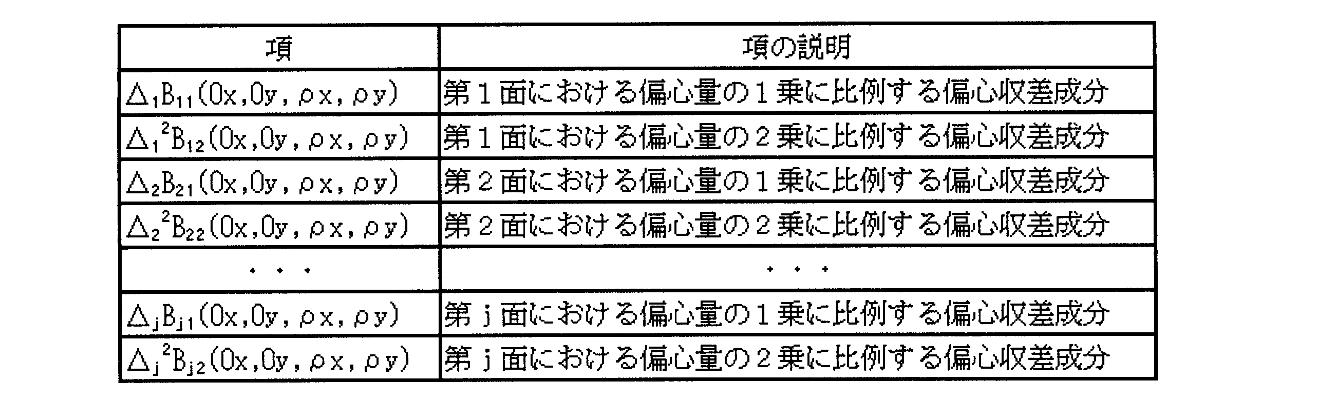
=1・B1jl(Ox,Oy)
+ρx・B2jl(Ox,Oy)
+ρy・B3jl(Ox,Oy)
+{2(ρx2+ρy2)-1}・B4jl(Ox,Oy)
+{ρx2-ρy2}・B5jl(Ox,Oy)
+2ρxρy・B6jl(Ox,Oy)
+{3(ρx2+ρy2)ρx-2ρx}・B7jl(Ox,Oy)
+{3(ρx2+ρy2)ρy-2ρy}・B8jl(Ox,Oy)
+{6(ρx2+ρy2)2-6(ρx2+ρy2)+1}・B9jl(Ox,Oy)
+・・・ (2)
ここで、
B1jl(Ox,Oy)~B9jl(Ox,Oy)は偏心収差感度、
である。
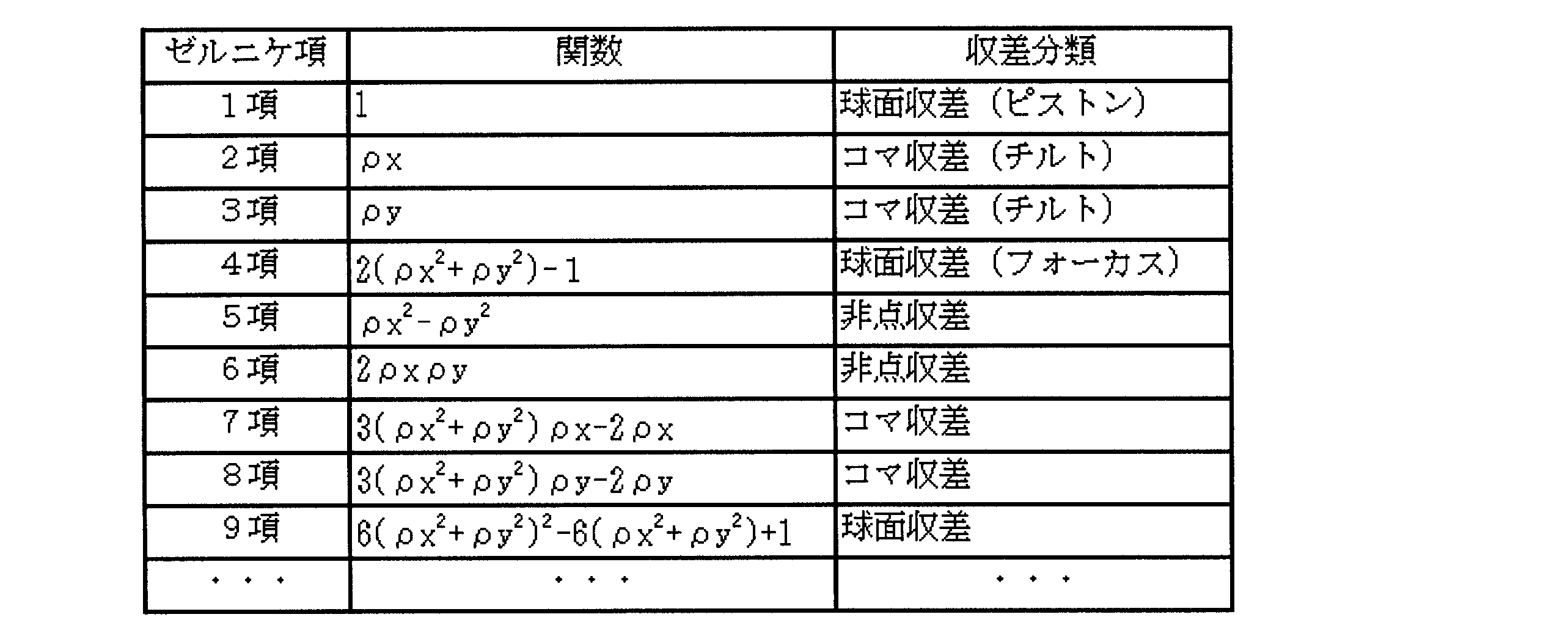
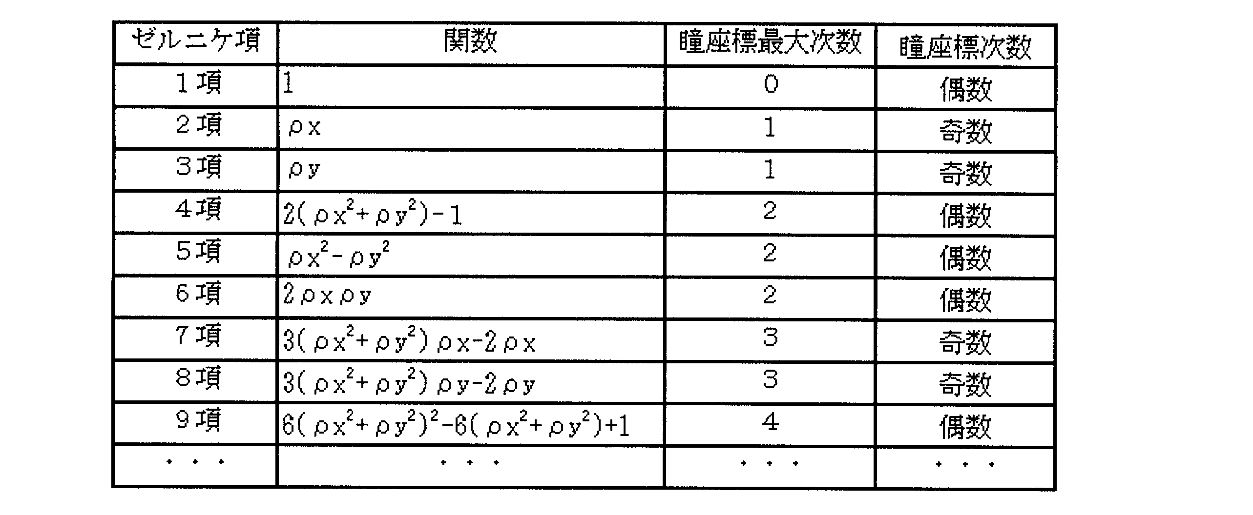
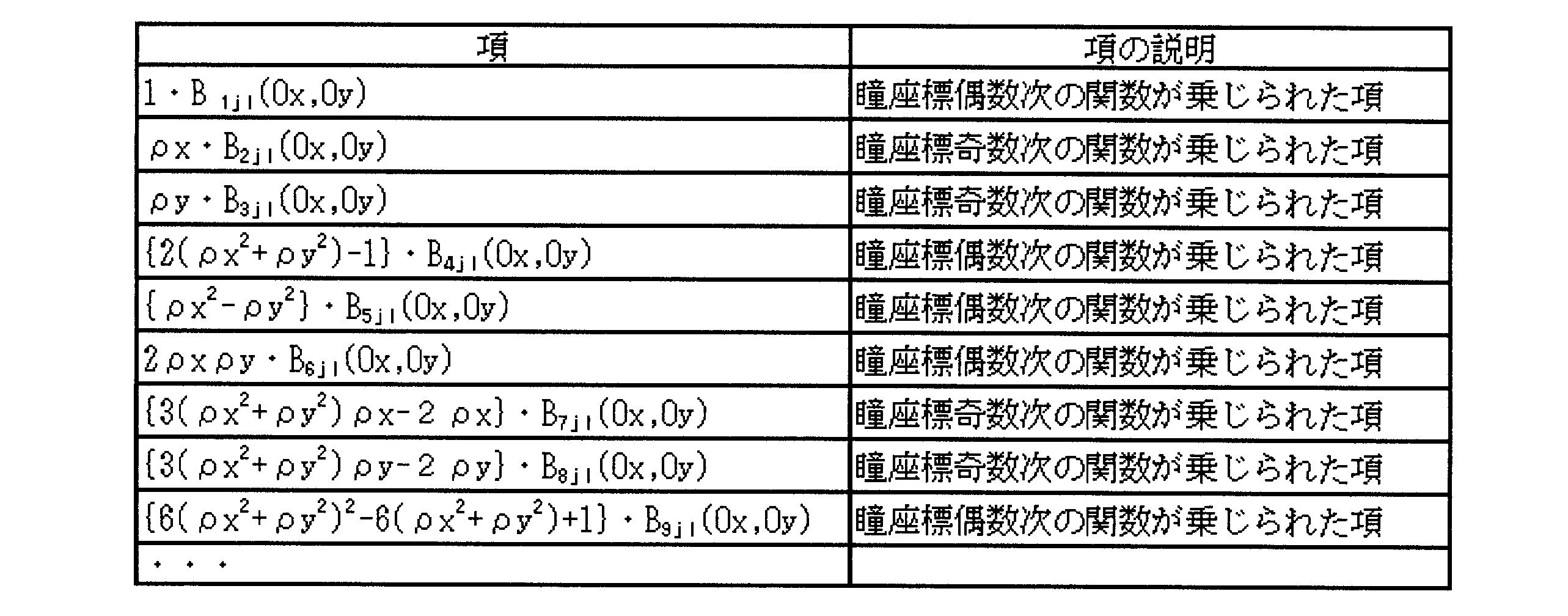
Bzj1(Ox,Oy)=Czj100+Czj120Ox2+Czj111OxOy+Czj102Oy2+・・・ (3)
Bzj1(Ox,Oy)=Czj110Ox+Czj101Oy+Czj130Ox3+Czj121Ox2Oy
+Czj112OxOy2+Czj103Oy3+・・・ (4)
Bzj2(Ox,Oy)=Czj210Ox+Czj201Oy+Czj230Ox3+Czj221Ox2Oy
+Czj212OxOy2+Czj203Oy3+・・・ (5)
Bzj2(Ox,Oy)=Czj200+Czj220Ox2+Czj211OxOy+Czj202Oy2+・・・ (6)
=1・W1(Ox,Oy,Δ1,Δ2,・・・,Δj)
+ρx・W2(Ox,Oy,Δ1,Δ2,・・・,Δj)
+ρy・W3(Ox,Oy,Δ1,Δ2,・・・,Δj)
+{2(ρx2+ρy2)-1}・W4(Ox,Oy,Δ1,Δ2,・・・,Δj)
+(ρx2-ρy2)・W5(Ox,Oy,Δ1,Δ2,・・・,Δj)
+2ρxρy・W6(Ox,Oy,Δ1,Δ2,・・・,Δj)
+{3(ρx2+ρy2)ρx-2ρx}・W7(Ox,Oy,Δ1,Δ2,・・・,Δj)
+{3(ρx2+ρy2)ρy-2ρy}・W8(Ox,Oy,Δ1,Δ2,・・・,Δj)
+{6(ρx2+ρy2)2-6(ρx2+ρy2)+1}・W9(Ox,Oy,Δ1,Δ2,・・・,Δj)
=f1(ρx,ρy)・W1(Ox,Oy,Δ1,Δ2,・・・,Δj)
+f2(ρx,ρy)・W2(Ox,Oy,Δ1,Δ2,・・・,Δj)
+f3(ρx,ρy)・W3(Ox,Oy,Δ1,Δ2,・・・,Δj)
+f4(ρx,ρy)・W4(Ox,Oy,Δ1,Δ2,・・・,Δj)
+f5(ρx,ρy)・W5(Ox,Oy,Δ1,Δ2,・・・,Δj)
+f6(ρx,ρy)・W6(Ox,Oy,Δ1,Δ2,・・・,Δj)
+f7(ρx,ρy)・W7(Ox,Oy,Δ1,Δ2,・・・,Δj)
+f8(ρx,ρy)・W8(Ox,Oy,Δ1,Δ2,・・・,Δj)
+f9(ρx,ρy)・W9(Ox,Oy,Δ1,Δ2,・・・,Δj) (7)
ここで、
W1~W9は収差成分、
f1(ρx,ρy)~f9(ρx,ρy)はゼルニケ項を表す関数、
である。
W(Ox,Oy,ρx,ρy,Δ1,Δ2,・・・,Δj)
=Δ1B11(Ox,Oy,ρx,ρy)
+Δ1 2B12(Ox,Oy,ρx,ρy)
+Δ2B21(Ox,Oy,ρx,ρy)
+Δ2 2B22(Ox,Oy,ρx,ρy)
+・・・
+ΔjBj1(Ox,Oy,ρx,ρy)
+Δj 2Bj2(Ox,Oy,ρx,ρy) (1)
=f1(ρx,ρy)・B1jl(Ox,Oy)+f2(ρx,ρy)・B2jl(Ox,Oy)+f3(ρx,ρy)・B3jl(Ox,Oy)
+f4(ρx,ρy)・B4jl(Ox,Oy)+・・・+f9(ρx,ρy)・B9jl(Ox,Oy) (2’)
W(Ox,Oy,ρx,ρy,Δ1,Δ2,・・・,Δj)
=Δ1{f1(ρx,ρy)・B111(Ox,Oy)+f2(ρx,ρy)・B211(Ox,Oy)+f3(ρx,ρy)・B311(Ox,Oy)
+f4(ρx,ρy)・B411(Ox,Oy)+・・・+f9(ρx,ρy)・B911(Ox,Oy)}
+Δ1 2{f1(ρx,ρy)・B112(Ox,Oy)+f2(ρx,ρy)・B212(Ox,Oy)+f3(ρx,ρy)・B312(Ox,Oy)
+f4(ρx,ρy)・B412(Ox,Oy)+・・・+f9(ρx,ρy)・B912(Ox,Oy)}
+Δ2{f1(ρx,ρy)・B121(Ox,Oy)+f2(ρx,ρy)・B221(Ox,Oy)+f3(ρx,ρy)・B321(Ox,Oy)
+f4(ρx,ρy)・B421(Ox,Oy)+・・・+f9(ρx,ρy)・B921(Ox,Oy)}
+Δ2 2{f1(ρx,ρy)・B122(Ox,Oy)+f2(ρx,ρy)・B222(Ox,Oy)+f3(ρx,ρy)・B322(Ox,Oy)
+f4(ρx,ρy)・B422(Ox,Oy)+・・・+f9(ρx,ρy)・B922(Ox,Oy)}
+・・・
+Δj{f1(ρx,ρy)・B1j1(Ox,Oy)+f2(ρx,ρy)・B2j1(Ox,Oy)+f3(ρx,ρy)・B3j1(Ox,Oy)
+f4(ρx,ρy)・B4j1(Ox,Oy)+・・・+f9(ρx,ρy)・B9j1(Ox,Oy)}
+Δj 2{f1(ρx,ρy)・B1j2(Ox,Oy)+f2(ρx,ρy)・B2j2(Ox,Oy)+f3(ρx,ρy)・B3j2(Ox,Oy)
+f4(ρx,ρy)・B4j2(Ox,Oy)+・・・+f9(ρx,ρy)・B9j2(Ox,Oy)}
(1-1)
W(Ox,Oy,ρx,ρy,Δ1,Δ2,・・・,Δj)
=f1(ρx,ρy)・[{Δ1B111(Ox,Oy)+Δ2B121(Ox,Oy)+・・・+ΔjB1j1(Ox,Oy)}
+{Δ1 2B112(Ox,Oy)+Δ2 2B122(Ox,Oy)+・・・+Δj 2B1j2(Ox,Oy)}]
+f2(ρx,ρy)・[{Δ1B211(Ox,Oy)+Δ2B221(Ox,Oy)+・・・+ΔjB2j1(Ox,Oy)}
+{Δ1 2B212(Ox,Oy)+Δ2 2B222(Ox,Oy)+・・・+Δj 2B2j2(Ox,Oy)}]
+f3(ρx,ρy)・[{Δ1B311(Ox,Oy)+Δ2B321(Ox,Oy)+・・・+ΔjB3j1(Ox,Oy)}
+{Δ1 2B312(Ox,Oy)+Δ2 2B322(Ox,Oy)+・・・+Δj 2B3j2(Ox,Oy)}]
+f4(ρx,ρy)・[{Δ1B411(Ox,Oy)+Δ2B421(Ox,Oy)+・・・+ΔjB4j1(Ox,Oy)}
+{Δ1 2B412(Ox,Oy)+Δ2 2B422(Ox,Oy)+・・・+Δj 2B4j2(Ox,Oy)}]
+・・・
+f9(ρx,ρy)・[{Δ1B911(Ox,Oy)+Δ2B921(Ox,Oy)+・・・+ΔjB9j1(Ox,Oy)}
+{Δ1 2B912(Ox,Oy)+Δ2 2B921(Ox,Oy)+・・・+Δj 2B9j2(Ox,Oy)}]
(1-2)
W1(Ox,Oy,Δ1,Δ2,・・・,Δj)
=[{Δ1B111(Ox,Oy)+Δ2B121(Ox,Oy)+・・・+ΔjB1j1(Ox,Oy)}
+{Δ1 2B112(Ox,Oy)+Δ2 2B122(Ox,Oy)+・・・+Δj 2B1j2(Ox,Oy)}] (8-1)
W2(Ox,Oy,Δ1,Δ2,・・・,Δj)
=[{Δ1B211(Ox,Oy)+Δ2B221(Ox,Oy)+・・・+ΔjB2j1(Ox,Oy)}
+{Δ1 2B212(Ox,Oy)+Δ2 2B222(Ox,Oy)+・・・+Δj 2B2j2(Ox,Oy)}] (8-2)
W3(Ox,Oy,Δ1,Δ2,・・・,Δj)
=[{Δ1B311(Ox,Oy)+Δ2B321(Ox,Oy)+・・・+ΔjB3j1(Ox,Oy)}
+{Δ1 2B312(Ox,Oy)+Δ2 2B322(Ox,Oy)+・・・+Δj 2B3j2(Ox,Oy)}] (8-3)
W4(Ox,OyΔ1,Δ2,・・・,Δj)
=[{Δ1B411(Ox,Oy)+Δ2B421(Ox,Oy)+・・・+ΔjB4j1(Ox,Oy)}
+{Δ1 2B412(Ox,Oy)+Δ2 2B422(Ox,Oy)+・・・+Δj 2B4j2(Ox,Oy)}] (8-4)
W5(Ox,Oy,Δ1,Δ2,・・・,Δj)
=[{Δ1B511(Ox,Oy)+Δ2B521(Ox,Oy)+・・・+ΔjB5j1(Ox,Oy)}
+{Δ1 2B512(Ox,Oy)+Δ2 2B522(Ox,Oy)+・・・+Δj 2B5j2(Ox,Oy)}] (8-5)
W6(Ox,Oy,Δ1,Δ2,・・・,Δj)
=[{Δ1B611(Ox,Oy)+Δ2B621(Ox,Oy)+・・・+ΔjB6j1(Ox,Oy)}
+{Δ1 2B612(Ox,Oy)+Δ2 2B622(Ox,Oy)+・・・+Δj 2B6j2(Ox,Oy)}] (8-6)
W7(Ox,Oy,Δ1,Δ2,・・・,Δj)
=[{Δ1B711(Ox,Oy)+Δ2B721(Ox,Oy)+・・・+ΔjB7j1(Ox,Oy)}
+{Δ1 2B712(Ox,Oy)+Δ2 2B722(Ox,Oy)+・・・+Δj 2B7j2(Ox,Oy)}] (8-7)
W8(Ox,Oy,Δ1,Δ2,・・・,Δj)
=[{Δ1B811(Ox,Oy)+Δ2B821(Ox,Oy)+・・・+ΔjB8j1(Ox,Oy)}
+{Δ1 2B812(Ox,Oy)+Δ2 2B822(Ox,Oy)+・・・+Δj 2B8j2(Ox,Oy)}] (8-8)
W9(Ox,Oy,Δ1,Δ2,・・・,Δj)
=[{Δ1B911(Ox,Oy)+Δ2B921(Ox,Oy)+・・・+ΔjB9j1(Ox,Oy)}
+{Δ1 2B912(Ox,Oy)+Δ2 2B922(Ox,Oy)+・・・+Δj 2B9j2(Ox,Oy)}] (8-9)
W11(Ox,Oy,Δ1,Δ2,・・・,Δj)
=Δ1B111(Ox,Oy)+Δ2B121(Ox,Oy)+・・・+ΔjB1j1(Ox,Oy) (9-1)
W21(Ox,Oy,Δ1,Δ2,・・・,Δj)
=Δ1B211(Ox,Oy)+Δ2B221(Ox,Oy)+・・・+ΔjB2j1(Ox,Oy) (9-2)
W31(Ox,Oy,Δ1,Δ2,・・・,Δj)
=Δ1B311(Ox,Oy)+Δ2B321(Ox,Oy)+・・・+ΔjB3j1(Ox,Oy) (9-3)
W41(Ox,Oy,Δ1,Δ2,・・・,Δj)
=Δ1B411(Ox,Oy)+Δ2B421(Ox,Oy)+・・・+ΔjB4j1(Ox,Oy) (9-4)
W51(Ox,Oy,Δ1,Δ2,・・・,Δj)
=Δ1B511(Ox,Oy)+Δ2B521(Ox,Oy)+・・・+ΔjB5j1(Ox,Oy) (9-5)
W61(Ox,Oy,Δ1,Δ2,・・・,Δj)
=Δ1B611(Ox,Oy)+Δ2B621(Ox,Oy)+・・・+ΔjB6j1(Ox,Oy) (9-6)
W71(Ox,Oy,Δ1,Δ2,・・・,Δj)
=Δ1B711(Ox,Oy)+Δ2B721(Ox,Oy)+・・・+ΔjB7j1(Ox,Oy) (9-7)
W81(Ox,Oy,Δ1,Δ2,・・・,Δj)
=Δ1B811(Ox,Oy)+Δ2B821(Ox,Oy)+・・・+ΔjB8j1(Ox,Oy) (9-8)
W91(Ox,Oy,Δ1,Δ2,・・・,Δj)
=Δ1B911(Ox,Oy)+Δ2B921(Ox,Oy)+・・・+ΔjB9j1(Ox,Oy) (9-9)
W11=Δ1B111+Δ2B121+・・・+ΔjB1j1 (10-1)
W21=Δ1B211+Δ2B221+・・・+ΔjB2j1 (10-2)
W31=Δ1B311+Δ2B321+・・・+ΔjB3j1 (10-3)
W41=Δ1B411+Δ2B421+・・・+ΔjB4j1 (10-4)
W51=Δ1B511+Δ2B521+・・・+ΔjB5j1 (10-5)
W61=Δ1B611+Δ2B621+・・・+ΔjB6j1 (10-6)
W71=Δ1B711+Δ2B721+・・・+ΔjB7j1 (10-7)
W81=Δ1B811+Δ2B821+・・・+ΔjB8j1 (10-8)
W91=Δ1B911+Δ2B921+・・・+ΔjB9j1 (10-9)
=[{Δ1B111(-Ox,-Oy)+Δ2B121(-Ox,-Oy)+・・・+ΔjB1j1(-Ox,-Oy)}
+{Δ1 2B112(-Ox,-Oy)+Δ2 2B122(-Ox,-Oy)+・・・+Δj 2B1j2(-Ox,-Oy)}] (8-1’)
W2(-Ox,-Oy,Δ1,Δ2,・・・,Δj)
=[{Δ1B211(-Ox,-Oy)+Δ2B221(-Ox,-Oy)+・・・+ΔjB2j1(-Ox,-Oy)}
+{Δ1 2B212(-Ox,-Oy)+Δ2 2B222(-Ox,-Oy)+・・・+Δj 2B2j2(-Ox,-Oy)}] (8-2’)
W3(-Ox,-Oy,Δ1,Δ2,・・・,Δj)
=[{Δ1B311(-Ox,-Oy)+Δ2B321(-Ox,-Oy)+・・・+ΔjB3j1(-Ox,-Oy)}
+{Δ1 2B312(-Ox,-Oy)+Δ2 2B322(-Ox,-Oy)+・・・+Δj 2B3j2(-Ox,-Oy)}] (8-3’)
W4(-Ox,-Oy,Δ1,Δ2,・・・,Δj)
=[{Δ1B411(-Ox,-Oy)+Δ2B421(-Ox,-Oy)+・・・+ΔjB4j1(-Ox,-Oy)}
+{Δ1 2B412(-Ox,-Oy)+Δ2 2B422(-Ox,-Oy)+・・・+Δj 2B4j2(-Ox,-Oy)}] (8-4’)
W5(-Ox,-Oy,Δ1,Δ2,・・・,Δj)
=[{Δ1B511(-Ox,-Oy)+Δ2B521(-Ox,-Oy)+・・・+ΔjB5j1(-Ox,-Oy)}
+{Δ1 2B512(-Ox,-Oy)+Δ2 2B522(-Ox,-Oy)+・・・+Δj 2B5j2(-Ox,-Oy)}] (8-5’)
W6(-Ox,-Oy,Δ1,Δ2,・・・,Δj)
=[{Δ1B611(-Ox,-Oy)+Δ2B621(-Ox,-Oy)+・・・+ΔjB6j1(-Ox,-Oy)}
+{Δ1 2B612(-Ox,-Oy)+Δ2 2B622(-Ox,-Oy)+・・・+Δj 2B6j2(-Ox,-Oy)}] (8-6’)
W7(-Ox,-Oy,Δ1,Δ2,・・・,Δj)
=[{Δ1B711(-Ox,-Oy)+Δ2B721(-Ox,-Oy)+・・・+ΔjB7j1(-Ox,-Oy)}
+{Δ1 2B712(-Ox,-Oy)+Δ2 2B722(-Ox,-Oy)+・・・+Δj 2B7j2(-Ox,-Oy)}] (8-7’)
W8(-Ox,-Oy,Δ1,Δ2,・・・,Δj)
=[{Δ1B811(-Ox,-Oy)+Δ2B821(-Ox,-Oy)+・・・+ΔjB8j1(-Ox,-Oy)}
+{Δ1 2B812(-Ox,-Oy)+Δ2 2B822(-Ox,-Oy)+・・・+Δj 2B8j2(-Ox,-Oy)}] (8-8’)
W9(-Ox,-Oy,Δ1,Δ2,・・・,Δj)
=[{Δ1B911(-Ox,-Oy)+Δ2B921(-Ox,-Oy)+・・・+ΔjB9j1(-Ox,-Oy)}
+{Δ1 2B912(-Ox,-Oy)+Δ2 2B922(-Ox,-Oy)+・・・+Δj 2B9j2(-Ox,-Oy)}] (8-9’)
W2(Ox,Oy,Δ1,Δ2,・・・,Δj)とW2(-Ox,-Oy,Δ1,Δ2,・・・,Δj)。
W4(Ox,Oy,Δ1,Δ2,・・・,Δj)とW4(-Ox,-Oy,Δ1,Δ2,・・・,Δj)。
=[{Δ1B211(Ox,Oy)+Δ2B221(Ox,Oy)+・・・+ΔjB2j1(Ox,Oy)}
+{Δ1 2B212(Ox,Oy)+Δ2 2B222(Ox,Oy)+・・・+Δj 2B2j2(Ox,Oy)}] (8-2)
W2(-Ox,-Oy,Δ1,Δ2,・・・,Δj)
=[{Δ1B211(-Ox,-Oy)+Δ2B221(-Ox,-Oy)+・・・+ΔjB2j1(-Ox,-Oy)}
+{Δ1 2B212(-Ox,-Oy)+Δ2 2B222(-Ox,-Oy)+・・・+Δj 2B2j2(-Ox,-Oy)}] (8-2’)


Bzj1(Ox,Oy)=Czj100+Czj120Ox2+Czj111OxOy+Czj102Oy2+・・・ (3)
B2j1(Ox,Oy) =C2j100+C2j120Ox2+C2j111OxOy+C2j102Oy2+・・・ (3’)
B2j1(-Ox,-Oy)=C2j100+C2j120Ox2+C2j111OxOy+C2j102Oy2+・・・ (3”)
Bzj2(Ox,Oy)=Czj210Ox+Czj201Oy+Czj230Ox3+Czj221Ox2Oy
+Czj212OxOy2+Czj203Oy3+・・・ (5)
B2j2(Ox,Oy) = C2j210Ox+C2j201Oy+C2j230Ox3+C2j221Ox2Oy
+C2j212OxOy2+C2j203Oy3+・・・ (5’)
B2j2(-Ox,-Oy)=-C2j210Ox-C2j201Oy-C2j230Ox3-C2j221Ox2Oy
-C2j212OxOy2-C2j203Oy3-・・・
=-{C2j210Ox+C2j201Oy+C2j230Ox3+C2j221Ox2Oy
+C2j212OxOy2+C2j203Oy3+・・・} (5”)
物体高座標に対して偶関数になっている。


W4(Ox,Oy,Δ1,Δ2,・・・,Δj)
=[{Δ1B411(Ox,Oy)+Δ2B421(Ox,Oy)+・・・+ΔjB4j1(Ox,Oy)}
+{Δ1 2B412(Ox,Oy)+Δ2 2B422(Ox,Oy)+・・・+Δj 2B4j2(Ox,Oy)}] (8-4)
W4(-Ox,-Oy,Δ1,Δ2,・・・,Δj)
=[{Δ1B411(-Ox,-Oy)+Δ2B421(-Ox,-Oy)+・・・+ΔjB4j1(-Ox,-Oy)}
+{Δ1 2B412(-Ox,-Oy)+Δ2 2B422(-Ox,-Oy)+・・・+Δj 2B4j2(-Ox,-Oy)}] (8-4’)


Bzj1(Ox,Oy)=Czj110Ox+Czj101Oy+Czj130Ox3+Czj121Ox2Oy
+Czj112OxOy2+Czj103Oy3+・・・ (4)
B4j1(Ox,Oy) = C4j110Ox+C4j101Oy+C4j130Ox3+C4j121Ox2Oy
+C4j112OxOy2+C4j103Oy3+・・・ (4’)
B4j1(-Ox,-Oy)=-C4j110Ox-C4j101Oy-C4j130Ox3-C4j121Ox2Oy
-C4j112OxOy2-C4j103Oy3-・・・
=-{C4j110Ox+C4j101Oy+C4j130Ox3+C4j121Ox2Oy
+C4j112OxOy2+C4j103Oy3+・・・} (4”)
Bzj2(Ox,Oy)=Czj200+Czj220Ox2+Czj211OxOy+Czj202Oy2+・・・ (6)
B4j2(Ox,Oy) =C4j200+C4j220Ox2+C4j211OxOy+C4j202Oy2+・・・ (6’)
B4j2(-Ox,-Oy)=C4j200+C4j220Ox2+C4j211OxOy+C4j202Oy2+・・・ (6”)


W2(Ox,Oy,Δ1,Δ2,・・・,Δj)+W2(-Ox,-Oy,Δ1,Δ2,・・・,Δj)
=2・{Δ1B211(Ox,Oy)+Δ2B221(Ox,Oy)+・・・+ΔjB2j1(Ox,Oy)} (11)
W21(Ox,Oy,Δ1,Δ2,・・・,Δj)
=Δ1B211(Ox,Oy)+Δ2B221(Ox,Oy)+・・・+ΔjB2j1(Ox,Oy) (9-2)
W2(Ox,Oy,Δ1,Δ2,・・・,Δj)+W2(-Ox,-Oy,Δ1,Δ2,・・・,Δj)
=2・{Δ1B211(Ox,Oy)+Δ2B221(Ox,Oy)+・・・+ΔjB2j1(Ox,Oy)}
=2・W21(Ox,Oy,Δ1,Δ2,・・・,Δj) (11’)
W4(Ox,Oy,Δ1,Δ2,・・・,Δj)-W4(-Ox,-Oy,Δ1,Δ2,・・・,Δj)
=2・{Δ1B411(Ox,Oy)+Δ2B421(Ox,Oy)+・・・+ΔjB4j1(Ox,Oy)} (12)
W41(Ox,Oy,Δ1,Δ2,・・・,Δj)
=Δ1B411(Ox,Oy)+Δ2B421(Ox,Oy)+・・・+ΔjB4j1(Ox,Oy) (9-4)
W4(Ox,Oy,Δ1,Δ2,・・・,Δj)-W4(-Ox,-Oy,Δ1,Δ2,・・・,Δj)
=2・{Δ1B411(Ox,Oy)+Δ2B421(Ox,Oy)+・・・+ΔjB4j1(Ox,Oy)}
=2・W41(Ox,Oy,Δ1,Δ2,・・・,Δj) (12’)

W3(Ox,Oy,Δ1,Δ2,・・・,Δj)とW3(-Ox,-Oy,Δ1,Δ2,・・・,Δj)。
W7(Ox,Oy,Δ1,Δ2,・・・,Δj)とW7(-Ox,-Oy,Δ1,Δ2,・・・,Δj)。
W8(Ox,Oy,Δ1,Δ2,・・・,Δj)とW8(-Ox,-Oy,Δ1,Δ2,・・・,Δj)。
このように、Wzのうち、瞳座標が奇数次数の関数が乗じられた収差成分、すなわち、ゼルニケ項の第2項等の関数が乗じられた収差成分Wzについては、以下のようになる(z=2,3,7,8・・・)。
Wz(Ox,Oy,Δ1,Δ2,・・・,Δj)+Wz(-Ox,-Oy,Δ1,Δ2,・・・,Δj)
=2Δ1Bz11(Ox,Oy)+・・・+2ΔjBzj1(Ox,Oy)
W5(Ox,Oy,Δ1,Δ2,・・・,Δj)とW5(-Ox,-Oy,Δ1,Δ2,・・・,Δj)。
W6(Ox,Oy,Δ1,Δ2,・・・,Δj)とW6(-Ox,-Oy,Δ1,Δ2,・・・,Δj)。
W9(Ox,Oy,Δ1,Δ2,・・・,Δj)とW9(-Ox,-Oy,Δ1,Δ2,・・・,Δj)。
このように、Wzのうち、瞳座標が偶数次数の関数が乗じられた収差成分、すなわち、ゼルニケ項の第4項等の関数が乗じられた収差成分Wzについては、以下のようになる(z=1,4,5,6,9・・・)。
Wz(Ox,Oy,Δ1,Δ2,・・・,Δj)-Wz(-Ox,-Oy,Δ1,Δ2,・・・,Δj)
=2Δ1Bz11(Ox,Oy)+・・・+2ΔjBzj1(Ox,Oy)
=M(Ox,Oy,ρx,ρy)
+Δ1B11(Ox,Oy,ρx,ρy)
+Δ1 2B12(Ox,Oy,ρx,ρy)
+Δ2B21(Ox,Oy,ρx,ρy)
+Δ2 2B22(Ox,Oy,ρx,ρy)
+・・・
+ΔjBj1(Ox,Oy,ρx,ρy)
+Δj 2Bj2(Ox,Oy,ρx,ρy) (1-3)
=1・M1(Ox,Oy)
+ρx・M2(Ox,Oy)
+ρy・M3(Ox,Oy)
+{2(ρx2+ρy2)-1}・M4(Ox,Oy)
+{ρx2-ρy2}・M5(Ox,Oy)
+2ρxρy・M6(Ox,Oy)
+{3(ρx2+ρy2)ρx-2ρx}・M7(Ox,Oy)
+{3(ρx2+ρy2)ρy-2ρy}・M8(Ox,Oy)
+{6(ρx2+ρy2)2-6(ρx2+ρy2)+1}・M9(Ox,Oy)
+・・・ (13)
ここで、
M1(Ox,Oy)~M9(Ox,Oy)は物体高座標に依存する関数、
である。
Mz(Ox,Oy)=Czm10Ox+Czm01Oy+Czm30Ox3+zm21Ox2Oy+Czm12OxOy2+Czm03Oy3+・・・ (14)
Mz(Ox,Oy)=Czm00+Czm20Ox2+Czm11OxOy+Czm02Oy2+・・・ (15)

=Sys(Ox,Oy,ρx,ρy)
+Δ1B11(Ox,Oy,ρx,ρy)
+Δ1 2B12(Ox,Oy,ρx,ρy)
+Δ2B21(Ox,Oy,ρx,ρy)
+Δ2 2B22(Ox,Oy,ρx,ρy)
+・・・
+ΔjBj1(Ox,Oy,ρx,ρy)
+Δj 2Bj2(Ox,Oy,ρx,ρy) (1-4)
W’(Ox,Oy,ρx,ρy)=Sys(Ox,Oy,ρx,ρy) (16)
W(Ox,Oy,ρx,ρy,Δ1,Δ2,・・・,Δj)-W’(Ox,Oy,ρx,ρy) (17)
=Sys(Ox,Oy,ρx,ρy)
+δ1B11(Ox,Oy,ρx,ρy)
+δ1 2B12(Ox,Oy,ρx,ρy)
+δ2B21(Ox,Oy,ρx,ρy)
+δ2 2B22(Ox,Oy,ρx,ρy)
+・・・
+δjBj1(Ox,Oy,ρx,ρy)
+δj 2Bj2(Ox,Oy,ρx,ρy) (1-5)
=Sys(Ox,Oy,ρx,ρy)
+(-δ1)B11(Ox,Oy,ρx,ρy)
+(-δ1)2B12(Ox,Oy,ρx,ρy)
+(-δ2)B21(Ox,Oy,ρx,ρy)
+(-δ2)2B22(Ox,Oy,ρx,ρy)
+・・・
+(-δj)Bj1(Ox,Oy,ρx,ρy)
+(-δj)2Bj2(Ox,Oy,ρx,ρy) (1-6)
W(Ox,Oy,ρx,ρy,δ1,δ2,・・・,δj)
-W(Ox,Oy,ρx,ρy,-δ1,-δ2,・・・,-δj) (18)
=δ1B11(Ox,Oy,ρx,ρy)
+δ1 2B12(Ox,Oy,ρx,ρy)
+δ2B21(Ox,Oy,ρx,ρy)
+δ2 2B22(Ox,Oy,ρx,ρy)
+・・・
+δjBj1(Ox,Oy,ρx,ρy)
+δj 2Bj2(Ox,Oy,ρx,ρy)
+δj+1B(j+1)1(Ox,Oy,ρx,ρy)
+δj+1 2B(j+1)2(Ox,Oy,ρx,ρy)
+δj+2B(j+2)1(Ox,Oy,ρx,ρy)
+δj+2 2B(j+2)2(Ox,Oy,ρx,ρy)
+・・・
+δmBm1(Ox,Oy,ρx,ρy)
+δm 2Bm2(Ox,Oy,ρx,ρy) (1-7)
=(-δ1)B11(Ox,Oy,ρx,ρy)
+(-δ1)2B12(Ox,Oy,ρx,ρy)
+(-δ2)B21(Ox,Oy,ρx,ρy)
+(-δ2)2B22(Ox,Oy,ρx,ρy)
+・・・
+(-δj)Bj1(Ox,Oy,ρx,ρy)
+(-δj)2Bj2(Ox,Oy,ρx,ρy)
+δj+1B(j+1)1(Ox,Oy,ρx,ρy)
+δj+1 2B(j+1)2(Ox,Oy,ρx,ρy)
+δj+2B(j+2)1(Ox,Oy,ρx,ρy)
+δj+2 2B(j+2)2(Ox,Oy,ρx,ρy)
+・・・
+δmBm1(Ox,Oy,ρx,ρy)
+δm 2Bm2(Ox,Oy,ρx,ρy) (1-8)

=(δ1+E)B11(Ox,Oy,ρx,ρy)
+(δ1+E)2B12(Ox,Oy,ρx,ρy)
+(δ2+E)B21(Ox,Oy,ρx,ρy)
+(δ2+E)2B22(Ox,Oy,ρx,ρy)
+・・・
+(δj+E)Bj1(Ox,Oy,ρx,ρy)
+(δj+E)2Bj2(Ox,Oy,ρx,ρy) (1-9)
=(-δ1+E)B11(Ox,Oy,ρx,ρy)
+(-δ1+E)2B12(Ox,Oy,ρx,ρy)
+(-δ2+E)B21(Ox,Oy,ρx,ρy)
+(-δ2+E)2B22(Ox,Oy,ρx,ρy)
+・・・
+(-δj+E)Bj1(Ox,Oy,ρx,ρy)
+(-δj+E)2Bj2(Ox,Oy,ρx,ρy) (1-10)
W(Ox,Oy,ρx,ρy,-δ1+E,-δ2+E、・・・,-δj+E)
-W(Ox,Oy,ρx,ρy,δ1+E,δ2+E、・・・,δj+E) (19)
W(Ox,Oy,ρx,ρy,-δ1+E,-δ2+E、・・・,-δj+E)
-W(Ox,Oy,ρx,ρy,δ1+E,δ2+E、・・・,δj+E)
=(-2δ1)B11(Ox,Oy,ρx,ρy)
+[(-δ1+E)2-(δ1+E)2]B12(Ox,Oy,ρx,ρy)
+(-2δ2)B21(Ox,Oy,ρx,ρy)
+[(-δ2+E)2-(δ2+E)2]B22(Ox,Oy,ρx,ρy)
+・・・
+(-2δj)Bj1(Ox,Oy,ρx,ρy)
+[(-δj+E)2-(δj+E)2]Bj2(Ox,Oy,ρx,ρy)
=(-2δ1)B11(Ox,Oy,ρx,ρy)
+(-4δ1E)B12(Ox,Oy,ρx,ρy)
+(-2δ2)B21(Ox,Oy,ρx,ρy)
+(-4δ2E)B22(Ox,Oy,ρx,ρy)
+・・・
+(-2δj)Bj1(Ox,Oy,ρx,ρy)
+(-4δjE)Bj2(Ox,Oy,ρx,ρy) (1-11)

W(-Ox,-Oy,ρx,ρy,δ1+E,δ2+E、・・・,δj+E)
-W(-Ox,-Oy,ρx,ρy,-δ1+E,-δ2+E、・・・,-δj+E)
=(-2δ1)B11(-Ox,-Oy,ρx,ρy)
+(-4δ1E)B12(-Ox,-Oy,ρx,ρy)
+(-2δ2)B21(-Ox,-Oy,ρx,ρy)
+(-4δ2E)B22(-Ox,-Oy,ρx,ρy)
+・・・
+(-2δj)Bj1(-Ox,-Oy,ρx,ρy)
+(-4δjE)Bj2(-Ox,-Oy,ρx,ρy) (1-12)
=[Wz(Ox,Oy,-δ1+E,-δ2+E、・・・,-δj+E)
‐Wz(Ox,Oy,δ1+E,δ2+E、・・・,δj+E)]
+[Wz(-Ox,-Oy,-δ1+E,-δ2+E、・・・,-δj+E)
‐Wz(-Ox,-Oy,δ1+E,δ2+E、・・・,δj+E)]
=(-2δ1)[Bz11(Ox,Oy)+Bz11(-Ox,-Oy)]
+(-4δ1E)[Bz12(Ox,Oy)+Bz12(-Ox,-Oy)]
+(-2δ2)[Bz21(Ox,Oy)+Bz21(-Ox,-Oy)]
+(-4δ2E)[Bz22(Ox,Oy)+Bz22(-Ox,-Oy)]
+・・・
+(-2δj)[Bzj1(Ox,Oy)+Bzj1(-Ox,-Oy)]
+(-4δjE)[Bzj2(Ox,Oy)+Bzj2(-Ox,-Oy)] (20)
Tz(Ox,Oy,δ1,δ2, ・・・,δj)
=(-2δ1)[2Bz11(Ox,Oy)]
+(-2δ2)[2Bz21(Ox,Oy)]
+・・・
+(-2δj)[2Bzj1(Ox,Oy)] (21)
=[Wz(Ox,Oy,-δ1+E,-δ2+E、・・・,-δj+E)
‐Wz(Ox,Oy,δ1+E,δ2+E、・・・,δj+E)]
‐[Wz(-Ox,-Oy,-δ1+E,-δ2+E、・・・,-δj+E)
‐Wz(-Ox,-Oy,δ1+E,δ2+E、・・・,δj+E)]
=(-2δ1)[Bz11(Ox,Oy)-Bz11(-Ox,-Oy)]
+(-4δ1E)[Bz12(Ox,Oy)-Bz12(-Ox,-Oy)]
+(-2δ2)[Bz21(Ox,Oy)-Bz21(-Ox,-Oy)]
+(-4δ2E)[Bz22(Ox,Oy)-Bz22(-Ox,-Oy)]
+・・・
+(-2δj)[Bzj1(Ox,Oy)-Bzj1(-Ox,-Oy)]
+(-4δjE)[Bzj2(Ox,Oy)-Bzj2(-Ox,-Oy)] (22)
Tz(Ox,Oy,δ1,δ2,・・・,δj)
=(-2δ1)[2Bz11(Ox,Oy)]
+(-2δ2)[2Bz21(Ox,Oy)]
+・・・
+(-2δj)[2Bzj1(Ox,Oy)] (23)
w11(Ox1,Oy1,Δ1,Δ2,・・・,Δj)
=Δ1B111(Ox1,Oy1)+Δ2B121(Ox1,Oy1)+・・・+ΔjB1j1(Ox1,Oy1) (9-1’)
w21(Ox1,Oy1,Δ1,Δ2,・・・,Δj)
=Δ1B211(Ox1,Oy1)+Δ2B221(Ox1,Oy1)+・・・+ΔjB2j1(Ox1,Oy1) (9-2’)
w31(Ox1,Oy1,Δ1,Δ2,・・・,Δj)
=Δ1B311(Ox1,Oy1)+Δ2B321(Ox1,Oy1)+・・・+ΔjB3j1(Ox1,Oy1) (9-3’)
w41(Ox1,Oy1,Δ1,Δ2,・・・,Δj)
=Δ1B411(Ox1,Oy1)+Δ2B421(Ox1,Oy1)+・・・+ΔjB4j1(Ox1,Oy1) (9-4’)
w51(Ox1,Oy1,Δ1,Δ2,・・・,Δj)
=Δ1B511(Ox1,Oy1)+Δ2B521(Ox1,Oy1)+・・・+ΔjB5j1(Ox1,Oy1) (9-5’)
w61(Ox1,Oy1,Δ1,Δ2,・・・,Δj)
=Δ1B611(Ox1,Oy1)+Δ2B621(Ox1,Oy1)+・・・+ΔjB6j1(Ox1,Oy1) (9-6’)
w71(Ox1,Oy1,Δ1,Δ2,・・・,Δj)
=Δ1B711(Ox1,Oy1)+Δ2B721(Ox1,Oy1)+・・・+ΔjB7j1(Ox1,Oy1) (9-7’)
w81(Ox1,Oy1,Δ1,Δ2,・・・,Δj)
=Δ1B811(Ox1,Oy1)+Δ2B821(Ox1,Oy1)+・・・+ΔjB8j1(Ox1,Oy1) (9-8’)
w91(Ox1,Oy1,Δ1,Δ2,・・・,Δj)
=Δ1B911(Ox1,Oy1)+Δ2B921(Ox1,Oy1)+・・・+ΔjB9j1(Ox1,Oy1) (9-9’)
w11(Ox2,Oy2,Δ1,Δ2,・・・,Δj)
=Δ1B111(Ox2,Oy2)+Δ2B121(Ox2,Oy2)+・・・+ΔjB1j1(Ox2,Oy2) (9-1”)
w21(Ox2,Oy2,Δ1,Δ2,・・・,Δj)
=Δ1B211(Ox2,Oy2)+Δ2B221(Ox2,Oy2)+・・・+ΔjB2j1(Ox2,Oy2) (9-2”)
w31(Ox2,Oy2,Δ1,Δ2,・・・,Δj)
=Δ1B311(Ox2,Oy2)+Δ2B321(Ox2,Oy2)+・・・+ΔjB3j1(Ox2,Oy2) (9-3”)
w41(Ox2,Oy2,Δ1,Δ2,・・・,Δj)
=Δ1B411(Ox2,Oy2)+Δ2B421(Ox2,Oy2)+・・・+ΔjB4j1(Ox2,Oy2) (9-4”)
w51(Ox2,Oy2,Δ1,Δ2,・・・,Δj)
=Δ1B511(Ox2,Oy2)+Δ2B521(Ox2,Oy2)+・・・+ΔjB5j1(Ox2,Oy2) (9-5”)
w61(Ox2,Oy2,Δ1,Δ2,・・・,Δj)
=Δ1B611(Ox2,Oy2)+Δ2B621(Ox2,Oy2)+・・・+ΔjB6j1(Ox2,Oy2) (9-6”)
w71(Ox2,Oy2,Δ1,Δ2,・・・,Δj)
=Δ1B711(Ox2,Oy2)+Δ2B721(Ox2,Oy2)+・・・+ΔjB7j1(Ox2,Oy2) (9-7”)
w81(Ox2,Oy2,Δ1,Δ2,・・・,Δj)
=Δ1B811(Ox2,Oy2)+Δ2B821(Ox2,Oy2)+・・・+ΔjB8j1(Ox2,Oy2) (9-8”)
w91(Ox2,Oy2,Δ1,Δ2,・・・,Δj)
=Δ1B911(Ox2,Oy2)+Δ2B921(Ox2,Oy2)+・・・+ΔjB9j1(Ox2,Oy2) (9-9”)
このようにすることで、偏心量Δの1乗に比例する量、すなわち第1の収差成分を抽出することができる。
Bzj1(Ox,Oy)=Czj100+Czj120Ox2+Czj111OxOy+Czj102Oy2+・・・ (3)
Bzj1(Ox,Oy)=Czj110Ox+Czj101Oy+Czj130Ox3+Czj121Ox2Oy
+Czj112OxOy2+Czj103Oy3+・・・ (4)
Bzj2(Ox,Oy)=Czj210Ox+Czj201Oy+Czj230Ox3+Czj221Ox2Oy
+Czj212OxOy2+Czj203Oy3+・・・ (5)
Bzj2(Ox,Oy)=Czj200+Czj220Ox2+Czj211OxOy+Czj202Oy2+・・・ (6)


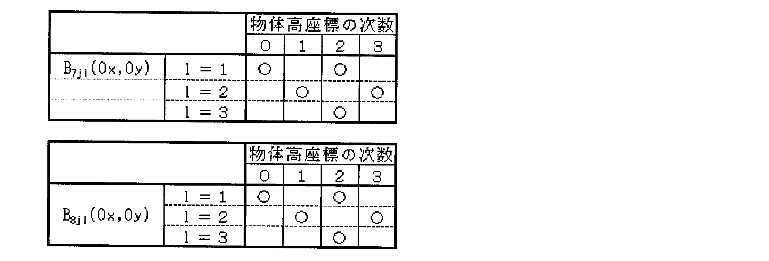
W(Ox,Oy,ρx,ρy,δ1+E,δ2+E、・・・,δj+E,δj+1,δj+2、・・・,δm)
=M(Ox,Oy,ρx,ρy)
+Sys(Ox,Oy,ρx,ρy)
+(δ1+E)B11(Ox,Oy,ρx,ρy)
+(δ1+E)2B12(Ox,Oy,ρx,ρy)
+(δ2+E)B21(Ox,Oy,ρx,ρy)
+(δ2+E)2B22(Ox,Oy,ρx,ρy)
+・・・
+(δj+E)Bj1(Ox,Oy,ρx,ρy)
+(δj+E)2Bj2(Ox,Oy,ρx,ρy)
+δj+1B(j+1)1(Ox,Oy,ρx,ρy)
+δj+1 2B(j+1)2(Ox,Oy,ρx,ρy)
+δj+2B(j+2)1(Ox,Oy,ρx,ρy)
+δj+2 2B(j+2)2(Ox,Oy,ρx,ρy)
+・・・
+δmBl1(Ox,Oy,ρx,ρy)
+δm 2Bl2(Ox,Oy,ρx,ρy) (1-13)
=M(Ox,Oy,ρx,ρy) (1-14)
=M(Ox,Oy,ρx,ρy)
+ΔoB11(Ox,Oy,ρx,ρy)
+Δo2B12(Ox,Oy,ρx,ρy) (1-15)
‐W(Ox,Oy,ρx,ρy,δ1=0,δ2=0、・・・,δm=0)
=ΔoB11(Ox,Oy,ρx,ρy)
+Δo2B12(Ox,Oy,ρx,ρy) (1-16)
‐W(-Ox,-Oy,ρx,ρy,δ1=0,δ2=0、・・・,δm=0)
=ΔoB11(-Ox,-Oy,ρx,ρy)
+Δo1 2B12(-Ox,-Oy,ρx,ρy) (1-17)
=[Wz(Ox,Oy,δ1=Δo=0.01,δ2=0、・・・,δm=0)‐W(Ox,Oy,ρx,ρy,δ1=0,δ2=0、・・・,δm=0)]
+[Wz(-Ox,-Oy,δ1=Δo=0.01,δ2=0、・・・,δm=0)‐W(-Ox,-Oy,ρx,ρy,δ1=0,δ2=0、・・・,δm=0)]
=Δo[2Bz11(Ox,Oy)] (24)
=[Wz(Ox,Oy,δ1=Δo=0.01,δ2=0、・・・,δm=0)‐W(Ox,Oy,ρx,ρy,δ1=0,δ2=0、・・・,δm=0)]
-[Wz(-Ox,-Oy,δ1=Δo=0.01,δ2=0、・・・,δm=0)‐W(-Ox,-Oy,ρx,ρy,δ1=0,δ2=0、・・・,δm=0)]
=Δo[2Bz11(Ox,Oy)] (25)
Bz11(Ox,Oy)=Sz1(Ox,Oy)/(2Δo) (25’)
W(Ox,Oy,δ1=Δo=0.01,δ2=0、・・・,δm=0)
W(Ox,Oy,ρx,ρy,δ1=0,δ2=0、・・・,δm=0)
W(-Ox,-Oy,δ1=Δo=0.01,δ2=0、・・・,δm=0)
W(-Ox,-Oy,ρx,ρy,δ1=0,δ2=0、・・・,δm=0)


Bzj1(Ox,Oy)=Czj100+Czj120Ox2+Czj111OxOy+Czj102Oy2+・・・ (3)
Bzj1(Ox,Oy)
=Dzj10・g0(Ox,Oy)+Dzj12・g2(Ox,Oy)+Dzj14・g4(Ox,Oy)+・・・ (26)
ここで、
g0(Ox,Oy)は、物体高座標の最大次数が0次の関数、
g2(Ox,Oy)は、物体高座標の最大次数が2次の関数、
g4(Ox,Oy)は、物体高座標の最大次数が4次の関数、
である。
Bzj1(Ox,Oy)=Czj110Ox+Czj101Oy+Czj130Ox3+Czj121Ox2Oy
+Czj112OxOy2+Czj103Oy3+・・・ (4)
Bzj1(Ox,Oy)
=Dzj11・g1(Ox,Oy)+Dzj13・g3(Ox,Oy)+Dzj15・g5(Ox,Oy)+・・・ (27)
ここで、
g1(Ox,Oy)は、物体高座標の最大次数が1次の関数、
g3(Ox,Oy)は、物体高座標の最大次数が3次の関数、
g5(Ox,Oy)は、物体高座標の最大次数が5次の関数、
である。
Tz(Ox,Oy,δ1,δ2,・・・,δj)/2
=Ez10・g0(Ox,Oy)+Ez12・g2(Ox,Oy)+Ez14+・g4(Ox,Oy)・・・ (28)
ここで、
g0(Ox,Oy)は、Ox,Oyのベキが最大次数0次の関数、
g2(Ox,Oy)は、Ox,Oyのベキが最大次数2次の関数、
g4(Ox,Oy)は、Ox,Oyのベキが最大次数4次の関数、
である。
Tz(Ox,Oy,δ1,δ2,・・・,δj)/2
=Ez11・g1(Ox,Oy)+Ez13・g3(Ox,Oy)+Ez15・g5(Ox,Oy)+・・・ (29)
ここで、
g1(Ox,Oy)は、Ox,Oyのベキが最大次数1次の関数、
g3(Ox,Oy)は、Ox,Oyのベキが最大次数3次の関数、
g5(Ox,Oy)は、Ox,Oyのベキが最大次数5次の関数、
である。

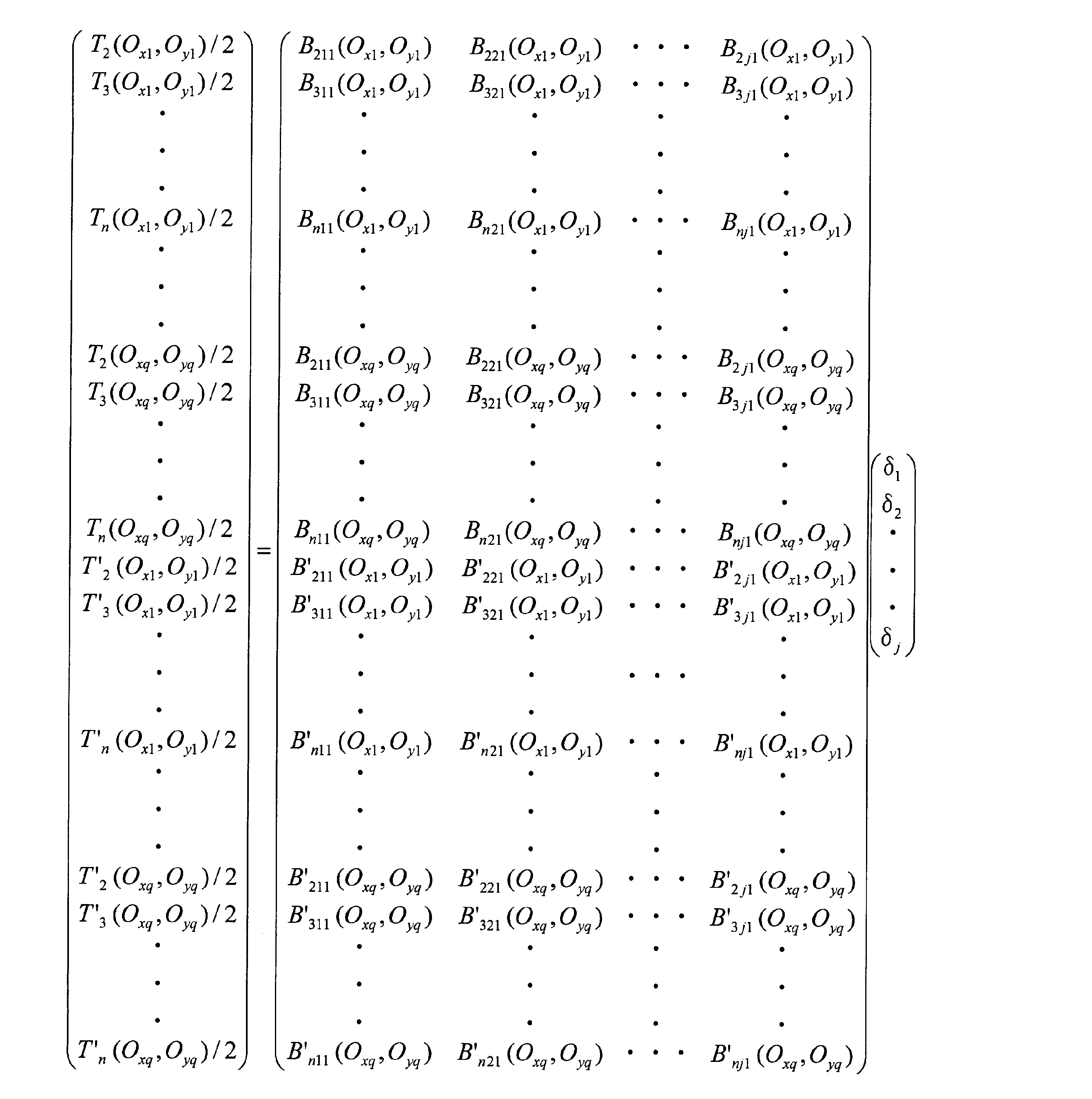

Sox(ρx,ρy)
=∂(Wo(ρx,ρy)+sys(ρx,ρy))/∂ρx・f
=∂Wo(ρx,ρy)/∂ρx+бsys(ρx,ρy)/∂ρx・f (30)
Soy(ρx,ρy)
=∂(Wo(ρx,ρy)+sys(ρx,ρy))/∂ρy・f
=∂Wo(ρx,ρy)/∂ρy+бsys(ρx,ρy)/∂ρy・f (31)
Sx(ρx,ρy)
=б(W(ρx,ρy)+sys(ρx,ρy))/∂ρx・f
=∂W(ρx,ρy)/∂ρx+∂sys(ρx,ρy)/∂ρx・f (32)
Sy(ρx,ρy)
=б(W(ρx,ρy)+sys(ρx,ρy))/∂ρy・f
=∂W(ρx,ρy)/∂ρy+∂sys(ρx,ρy)/∂ρy・f (33)
Sx(ρx,ρy)-Sox(ρx,ρy)
=∂(W(ρx,ρy)-Wo(ρx, ρy))/∂ρx・f (34)
Sy(ρx,ρy)-Soy(ρx,ρy)
=∂(W(ρx,ρy)-Wo(ρx,ρy))/∂ρy・f (35)
S2x(ρx,ρy)-S1x(ρx,ρy)
=∂(W2(ρx,ρy)-W1(ρx,ρy))/∂ρx・f (36)
S2y(ρx,ρy)-S1y(ρx, ρy)
=∂(W2(ρx,ρy)-W1(ρx,ρy))/∂ρy・f (37)
2、20、22 被検光学系
3、30 受光系
4 球面波
7、7’、8、8’、90、9’0、91、9’1 非平面波
21 光学系
23、24、25 レンズ
31 センサー部品構成部
32 波面データ取得部
33 受光素子
40 球面波
50、51、52、54、55、56 非平面波
53 平面波
60 歪んだ波面
70、71、72、73 球心
80 新たな軸
90 被検光学系
91 非球面
92、92’、94 非球面面頂
93 非球面軸
95 変位
96 球心
100 偏心量計測装置
101 本体部
102 投光系
103 受光系、波面計測装置
104 保持部材
105 被検光学系
106 保持部材
107 駆動ステージ
108 駆動ステージ
109 保持部材
110 移動機構
111 保持部材
111a 円環部
111b 回転機構
112 処理装置
113 ケーブル
120 SHセンサー
121 マイクロレンズアレイ
121a 基板
121b マイクロレンズ
122 撮像素子
130 投光系
131 光源
132 光ファイバー
133 出射部
140 投光系
141 基板
142 光源
150 Vブロック
151 治具
152 回転モータ
160 投光系
161 光源
162 光学系
163、164 レンズ
170 被検光学系
180 受光系
181 光学系
182、183 レンズ
184 波面計測装置
185、186 光束
190 被検光学系
200 偏心量計測装置
210 平面波
220 被検光学系
230 レンズ
240、260 偏心量計測装置
250 球面波
270 軸
AXM 計測軸
AXR1 第1の回転軸
AXR2 第2の回転軸
CR 中心光線
E シフト量
LS1、LS2、LS3 レンズ面
LS1、LS2、LSj レンズ面
L1、L2 レンズ
L11、L12、L21、L22 レンズ面
IM1、IM2、IM3 像
OB 物体
X、Y、A、B 偏心自由度
SC1、SC2、・・・、SCj、SCj+1、SCj+2、・・・、SCm 球心
δ1、δ2、・・・、δj、δj+1、δj+2、・・・、δm Y方向のシフト量
Claims (17)
- 計測軸上に配置された被検光学系に光束を照射して、偏心量を計測する方法であって、
前記被検光学系から出射した前記光束に基づいて波面データを取得する取得工程と、
前記波面データから所定の収差成分を抽出する第1の抽出工程と、
前記所定の収差成分から第1の収差成分を抽出する第2の抽出工程と、
前記第1の収差成分、偏心収差感度及び偏心量についての連立1次方程式を解析する解析工程と、を備え、
前記所定の収差成分は、偏心によって生じる収差成分が含まれる収差成分であり、
前記第1の収差成分は、前記所定の収差成分のうちの偏心量の1乗に比例する収差成分であり、
前記偏心収差感度は、偏心量の1乗に比例する収差感度であることを特徴とする偏心量計測方法。 - 前記取得工程では、2つの照射位置から前記光束が照射され、
前記2つの照射位置は前記計測軸に対して対称になっており、
前記第1の抽出工程は、一方の照射位置における波面データと他方の照射位置における波面データの各々から、前記所定の収差成分を抽出することを特徴とする請求項1に記載の偏心量計測方法。 - 前記所定の収差成分は第2の収差成分を含んでおり、
前記第2の収差成分は、前記所定の収差成分のうちの偏心量の2乗に比例する収差成分であり、
物体高座標は前記照射位置を表す座標であり、
所定の関数は前記第2の収差成分を表す関数であって、前記物体高座標を変数として含んでいる関数であり、
前記第2の抽出工程は、第1の演算工程と第2の演算工程とを有し、
前記第1の演算工程では、前記所定の関数が奇関数の場合に、前記一方の照射位置における前記所定の収差成分と、前記他方の照射位置における前記所定の収差成分との和をとり、
前記第2の演算工程では、前記所定の関数が偶関数の場合に、前記一方の照射位置における前記所定の収差成分と、前記他方の照射位置における前記所定の収差成分との差をとることを特徴とする請求項2に記載の偏心量計測方法。 - 前記取得工程は第1の回転を含み、
前記第1の回転では、前記計測軸の周りに前記被検光学系を回転させ、
同一の前記照射位置で、前記第1の回転前の波面データと、前記第1の回転後の波面データと、を取得することを特徴とする請求項2または3に記載の偏心量計測方法。 - 前記取得工程は第1の回転を含み、
前記第1の回転では、前記計測軸と平行な軸の周りに前記被検光学系を回転させ、
同一の前記照射位置で、前記第1の回転前の波面データと、前記第1の回転後の波面データと、を取得することを特徴とする請求項2または3に記載の偏心量計測方法。 - 前記被検光学系を回転させる角度が10度以上であることを特徴とする請求項4または5に記載の偏心量計測方法。
- 前記被検光学系を回転させる角度が180度であることを特徴とする請求項6に記載の偏心量計測方法。
- 前記一方の照射位置と前記他方の照射位置とをそれぞれ移動させ、移動後の照射位置で前記波面データを取得することを特徴とする請求項2から7のいずれか一項に記載の偏心量計測方法。
- 前記一方の照射位置を移動させ、移動後の照射位置で前記波面データを全て取得し、
その後、前記他方の照射位置を移動させ、移動後の照射位置で前記波面データを全て取得することを特徴とする請求項8に記載の偏心量計測方法。 - 前記一方の照射位置と前記他方の照射位置の各々で前記波面データを取得し、
その後、前記一方の照射位置と前記他方の照射位置を移動させ、移動後の照射位置の各々で前記波面データを取得することを特徴とする請求項8に記載の偏心量計測方法。 - 第1の照射状態で前記波面データの取得が行われ、
前記第1の照射状態では、前記光束の中心光線が前記計測軸と平行であることを特徴とする請求項1から10のいずれか一項に記載の偏心量計測方法。 - 第2の照射状態で前記波面データの取得が行われ、
前記第2の照射状態では、前記光束の中心光線が前記計測軸と所定の角度で交わることを特徴とする請求項1から10のいずれか一項に記載の偏心量計測方法。 - 前記第2の抽出工程は、所定の関数系を用いて行われ、
前記所定の関数系は、前記第1の収差成分を示す関数系であって、
一方の照射位置における前記所定の収差成分と、他方の照射位置における前記所定の収差成分とを、前記所定の関数系に当てはめることを特徴とする請求項1に記載の偏心量計測方法。 - 前記取得工程は第2の回転を含み、
前記第2の回転では、前記計測軸と直交する軸の周りに前記被検光学系を180度回転させ、
前記第2の回転前の波面データと、前記第2の回転後の波面データと、を取得することを特徴とする請求項1から13のいずれか一項に記載の偏心量計測方法。 - 前記第2の回転前の波面データの取得時における偏心量と、前記第2の回転後の波面データの取得時における偏心量とは、両者の絶対値が同一であることを特徴とする請求項14に記載の偏心量計測方法。
- 前記第1の抽出工程は、ゼルニケ多項式を用いて行われ、
前記所定の収差成分は、ゼルニケ多項式の係数であることを特徴とする請求項1から15のいずれか一項に記載の偏心量計測方法。 - 計測軸の一端に配置された投光系と、
前記計測軸の他端に配置された受光系と、
被検光学系を保持する保持部材と、
波面計測装置に接続された処理装置と、を備え、
前記保持部材は、前記投光系と前記受光系との間に配置され、
前記投光系は、前記被検光学系に光束を照射する位置に設けられ、
前記処理装置では、取得工程と、第1の抽出工程と、第2の抽出工程と、解析工程が実行され、
前記取得工程では、前記被検光学系から出射した前記光束に基づいて波面データが取得され、
前記第1の抽出工程では、前記波面データから所定の収差成分が抽出され、
前記第2の抽出工程では、前記所定の収差成分から第1の収差成分が抽出され、
前記解析工程では、前記第1の収差成分、偏心収差感度及び偏心量についての連立1次方程式が解析され、
前記所定の収差成分は、偏心によって生じる収差成分が含まれる収差成分であり、
前記第1の収差成分は、前記所定の収差成分のうちの偏心量の1乗に比例する収差成分であり、
前記偏心収差感度は、偏心量の1乗に比例する収差感度であることを特徴とする偏心量計測装置。
Priority Applications (3)
| Application Number | Priority Date | Filing Date | Title |
|---|---|---|---|
| CN201580036032.XA CN106471351B (zh) | 2014-07-03 | 2015-03-25 | 偏心量计测方法和偏心量计测装置 |
| DE112015002718.1T DE112015002718T5 (de) | 2014-07-03 | 2015-03-25 | Verfahren zur Messung eines Exzentrizitätsbetrags und Vorrichtung zur Messung eines Exzentrizitätsbetrags |
| JP2015544252A JP5870234B1 (ja) | 2014-07-03 | 2015-03-25 | 偏心量計測方法及び偏心量計測装置 |
Applications Claiming Priority (2)
| Application Number | Priority Date | Filing Date | Title |
|---|---|---|---|
| JP2014137980 | 2014-07-03 | ||
| JP2014-137980 | 2014-07-03 |
Publications (1)
| Publication Number | Publication Date |
|---|---|
| WO2016002272A1 true WO2016002272A1 (ja) | 2016-01-07 |
Family
ID=55018831
Family Applications (1)
| Application Number | Title | Priority Date | Filing Date |
|---|---|---|---|
| PCT/JP2015/059056 Ceased WO2016002272A1 (ja) | 2014-07-03 | 2015-03-25 | 偏心量計測方法及び偏心量計測装置 |
Country Status (4)
| Country | Link |
|---|---|
| JP (2) | JP5870234B1 (ja) |
| CN (1) | CN106471351B (ja) |
| DE (1) | DE112015002718T5 (ja) |
| WO (1) | WO2016002272A1 (ja) |
Cited By (2)
| Publication number | Priority date | Publication date | Assignee | Title |
|---|---|---|---|---|
| CN115638740A (zh) * | 2021-07-19 | 2023-01-24 | 中国科学院长春光学精密机械与物理研究所 | 一种多角度快速调节光学元件的装置及方法 |
| EP4130856A4 (en) * | 2020-03-23 | 2024-05-15 | Hoya Lens Thailand Ltd. | LENS EVALUATION METHODS, LENS DESIGN METHODS, LENS MANUFACTURING METHODS AND LENS EVALUATION PROGRAM |
Families Citing this family (4)
| Publication number | Priority date | Publication date | Assignee | Title |
|---|---|---|---|---|
| CN106247997B (zh) * | 2016-08-09 | 2018-12-28 | 中国人民解放军国防科学技术大学 | 用于正交导轨平台的垂直度误差测量方法 |
| CN110793754A (zh) * | 2019-11-01 | 2020-02-14 | 中国科学院光电技术研究所 | 一种基于相移调制的拼接式望远镜系统偏心误差探测方法 |
| CN116296273A (zh) * | 2021-12-21 | 2023-06-23 | 成都极米科技股份有限公司 | 多复眼元件对准方法、系统、装置、计算机设备及介质 |
| FR3134179B1 (fr) * | 2022-04-01 | 2025-07-18 | Fogale Nanotech | Procédé et système de caractérisation d’un objectif optique pour la correction d’aberrations optiques introduites par ledit objectif optique dans une image. |
Citations (8)
| Publication number | Priority date | Publication date | Assignee | Title |
|---|---|---|---|---|
| JP2001147174A (ja) * | 1999-11-19 | 2001-05-29 | Olympus Optical Co Ltd | 干渉測定機 |
| JP2003257812A (ja) * | 2002-02-27 | 2003-09-12 | Nikon Corp | 結像光学系の評価方法、結像光学系の調整方法、露光装置および露光方法 |
| JP2005024504A (ja) * | 2003-07-03 | 2005-01-27 | Olympus Corp | 偏心測定方法、偏心測定装置、及びこれらにより測定された物 |
| JP2007033343A (ja) * | 2005-07-28 | 2007-02-08 | Hoya Corp | 偏心測定方法、偏心測定装置、非球面単レンズの製造方法、非球面単レンズ及び光学機器 |
| JP2012163899A (ja) * | 2011-02-09 | 2012-08-30 | Mitsubishi Electric Corp | 光学調整装置及び光学調整方法 |
| JP2013195410A (ja) * | 2012-03-23 | 2013-09-30 | Olympus Corp | 検出装置及び検出方法 |
| JP2014020881A (ja) * | 2012-07-17 | 2014-02-03 | Olympus Corp | レンズ検査装置およびレンズ検査方法 |
| JP2014115077A (ja) * | 2011-03-31 | 2014-06-26 | Fujifilm Corp | レンズの面ズレ・面倒れを測定するレンズ測定方法及び装置 |
Family Cites Families (4)
| Publication number | Priority date | Publication date | Assignee | Title |
|---|---|---|---|---|
| JP4943946B2 (ja) * | 2007-06-04 | 2012-05-30 | 富士フイルム株式会社 | 偏芯量測定装置 |
| CN101236362B (zh) * | 2008-01-29 | 2010-06-23 | 北京理工大学 | 光刻机投影物镜波像差在线检测方法 |
| JP5399304B2 (ja) * | 2010-03-23 | 2014-01-29 | 富士フイルム株式会社 | 非球面体測定方法および装置 |
| CN102207378B (zh) * | 2011-03-09 | 2012-11-14 | 浙江大学 | 球面干涉检测中基于波前差分的高精度调整误差校正方法 |
-
2015
- 2015-03-25 JP JP2015544252A patent/JP5870234B1/ja active Active
- 2015-03-25 DE DE112015002718.1T patent/DE112015002718T5/de not_active Withdrawn
- 2015-03-25 WO PCT/JP2015/059056 patent/WO2016002272A1/ja not_active Ceased
- 2015-03-25 CN CN201580036032.XA patent/CN106471351B/zh active Active
-
2016
- 2016-01-06 JP JP2016001147A patent/JP6072317B2/ja active Active
Patent Citations (8)
| Publication number | Priority date | Publication date | Assignee | Title |
|---|---|---|---|---|
| JP2001147174A (ja) * | 1999-11-19 | 2001-05-29 | Olympus Optical Co Ltd | 干渉測定機 |
| JP2003257812A (ja) * | 2002-02-27 | 2003-09-12 | Nikon Corp | 結像光学系の評価方法、結像光学系の調整方法、露光装置および露光方法 |
| JP2005024504A (ja) * | 2003-07-03 | 2005-01-27 | Olympus Corp | 偏心測定方法、偏心測定装置、及びこれらにより測定された物 |
| JP2007033343A (ja) * | 2005-07-28 | 2007-02-08 | Hoya Corp | 偏心測定方法、偏心測定装置、非球面単レンズの製造方法、非球面単レンズ及び光学機器 |
| JP2012163899A (ja) * | 2011-02-09 | 2012-08-30 | Mitsubishi Electric Corp | 光学調整装置及び光学調整方法 |
| JP2014115077A (ja) * | 2011-03-31 | 2014-06-26 | Fujifilm Corp | レンズの面ズレ・面倒れを測定するレンズ測定方法及び装置 |
| JP2013195410A (ja) * | 2012-03-23 | 2013-09-30 | Olympus Corp | 検出装置及び検出方法 |
| JP2014020881A (ja) * | 2012-07-17 | 2014-02-03 | Olympus Corp | レンズ検査装置およびレンズ検査方法 |
Cited By (2)
| Publication number | Priority date | Publication date | Assignee | Title |
|---|---|---|---|---|
| EP4130856A4 (en) * | 2020-03-23 | 2024-05-15 | Hoya Lens Thailand Ltd. | LENS EVALUATION METHODS, LENS DESIGN METHODS, LENS MANUFACTURING METHODS AND LENS EVALUATION PROGRAM |
| CN115638740A (zh) * | 2021-07-19 | 2023-01-24 | 中国科学院长春光学精密机械与物理研究所 | 一种多角度快速调节光学元件的装置及方法 |
Also Published As
| Publication number | Publication date |
|---|---|
| DE112015002718T5 (de) | 2017-03-02 |
| JP6072317B2 (ja) | 2017-02-01 |
| JPWO2016002272A1 (ja) | 2017-04-27 |
| CN106471351A (zh) | 2017-03-01 |
| JP2016095316A (ja) | 2016-05-26 |
| JP5870234B1 (ja) | 2016-02-24 |
| CN106471351B (zh) | 2019-04-19 |
Similar Documents
| Publication | Publication Date | Title |
|---|---|---|
| JP6072317B2 (ja) | 偏心量計測方法及び偏心量計測装置 | |
| JP6494205B2 (ja) | 波面計測方法、形状計測方法、光学素子の製造方法、光学機器の製造方法、プログラム、波面計測装置 | |
| JP5399304B2 (ja) | 非球面体測定方法および装置 | |
| JP5971965B2 (ja) | 面形状計測方法、面形状計測装置、プログラム、および、光学素子の製造方法 | |
| CN113776460B (zh) | 检测光学自由曲面反射镜面形的方法及装置 | |
| CN106646867B (zh) | 一种深紫外光学系统共焦对准装置与方法 | |
| JP2010281792A (ja) | 非球面体測定方法および装置 | |
| KR20110065365A (ko) | 비구면체 측정 방법 및 장치 | |
| US11892283B2 (en) | Measuring apparatus for interferometrically determining a surface shape | |
| US10444112B2 (en) | Wavefront measurement apparatus and wavefront measurement method | |
| JP5591063B2 (ja) | 測定方法及び測定装置 | |
| US20200141832A1 (en) | Eccentricity measuring method, lens manufacturing method, and eccentricity measuring apparatus | |
| CN110702036B (zh) | 一种复光束角度传感器及小型非球面形貌检测方法 | |
| JP5904896B2 (ja) | レンズ検査装置およびレンズ検査方法 | |
| JP6558975B2 (ja) | 形状計測方法、形状計測装置および形状計測プログラム | |
| JP7446911B2 (ja) | 波面計測装置、波面計測方法、並びに、光学系および光学素子の製造方法 | |
| JP6445755B2 (ja) | 面形状測定装置または波面収差測定装置 | |
| WO2024202476A1 (ja) | レンズ測定方法及びレンズ測定装置 | |
| CN119714111A (zh) | 一种cgh和反射镜综合检测凸非球面的系统及方法 | |
| JP2017072447A (ja) | 位置算出方法、形状計測方法、形状計測装置、プログラム、記録媒体及び部品の製造方法 | |
| JP2021001746A (ja) | 形状計測方法、レンズの製造方法、および形状計測装置 | |
| Qin et al. | Research on Hartmann test for progressive addition lenses | |
| JP2021001747A (ja) | 偏心計測方法、レンズの製造方法、および偏心計測装置 | |
| King | A new approach to stitching optical metrology data | |
| JP2012225705A (ja) | 光学測定装置及び光学測定方法 |
Legal Events
| Date | Code | Title | Description |
|---|---|---|---|
| ENP | Entry into the national phase |
Ref document number: 2015544252 Country of ref document: JP Kind code of ref document: A |
|
| 121 | Ep: the epo has been informed by wipo that ep was designated in this application |
Ref document number: 15814200 Country of ref document: EP Kind code of ref document: A1 |
|
| WWE | Wipo information: entry into national phase |
Ref document number: 112015002718 Country of ref document: DE |
|
| 122 | Ep: pct application non-entry in european phase |
Ref document number: 15814200 Country of ref document: EP Kind code of ref document: A1 |