US8553228B2 - Web inspection calibration system and related methods - Google Patents
Web inspection calibration system and related methods Download PDFInfo
- Publication number
- US8553228B2 US8553228B2 US13/249,468 US201113249468A US8553228B2 US 8553228 B2 US8553228 B2 US 8553228B2 US 201113249468 A US201113249468 A US 201113249468A US 8553228 B2 US8553228 B2 US 8553228B2
- Authority
- US
- United States
- Prior art keywords
- web
- sensor
- inspection system
- cross
- calibration
- Prior art date
- Legal status (The legal status is an assumption and is not a legal conclusion. Google has not performed a legal analysis and makes no representation as to the accuracy of the status listed.)
- Active, expires
Links
- 238000007689 inspection Methods 0.000 title claims abstract description 181
- 238000000034 method Methods 0.000 title abstract description 83
- 238000001228 spectrum Methods 0.000 claims abstract description 26
- 230000004044 response Effects 0.000 claims description 60
- 238000005259 measurement Methods 0.000 claims description 38
- 239000000463 material Substances 0.000 claims description 18
- 238000004422 calculation algorithm Methods 0.000 claims description 15
- 238000006243 chemical reaction Methods 0.000 claims description 4
- 238000012544 monitoring process Methods 0.000 claims description 3
- 238000004458 analytical method Methods 0.000 abstract description 14
- 230000008569 process Effects 0.000 description 30
- 239000010408 film Substances 0.000 description 26
- 230000003287 optical effect Effects 0.000 description 25
- 238000000576 coating method Methods 0.000 description 24
- 238000003384 imaging method Methods 0.000 description 24
- 239000011248 coating agent Substances 0.000 description 22
- 239000011159 matrix material Substances 0.000 description 20
- 230000000875 corresponding effect Effects 0.000 description 18
- 239000000523 sample Substances 0.000 description 18
- 239000000758 substrate Substances 0.000 description 17
- 238000013459 approach Methods 0.000 description 16
- 238000004519 manufacturing process Methods 0.000 description 15
- 230000005540 biological transmission Effects 0.000 description 14
- 230000003595 spectral effect Effects 0.000 description 14
- 239000013598 vector Substances 0.000 description 13
- 230000006870 function Effects 0.000 description 12
- 238000005286 illumination Methods 0.000 description 12
- 230000000737 periodic effect Effects 0.000 description 12
- 230000008859 change Effects 0.000 description 11
- 230000002596 correlated effect Effects 0.000 description 11
- 238000012545 processing Methods 0.000 description 10
- 230000008033 biological extinction Effects 0.000 description 9
- 230000000694 effects Effects 0.000 description 8
- 238000012417 linear regression Methods 0.000 description 7
- 238000005070 sampling Methods 0.000 description 7
- 230000007547 defect Effects 0.000 description 6
- 238000012546 transfer Methods 0.000 description 6
- 238000003908 quality control method Methods 0.000 description 4
- 238000010521 absorption reaction Methods 0.000 description 3
- 238000004364 calculation method Methods 0.000 description 3
- 239000006229 carbon black Substances 0.000 description 3
- 230000006866 deterioration Effects 0.000 description 3
- 238000006073 displacement reaction Methods 0.000 description 3
- 238000009826 distribution Methods 0.000 description 3
- 230000009466 transformation Effects 0.000 description 3
- 238000012935 Averaging Methods 0.000 description 2
- 235000013405 beer Nutrition 0.000 description 2
- 230000008901 benefit Effects 0.000 description 2
- 238000012937 correction Methods 0.000 description 2
- 238000010219 correlation analysis Methods 0.000 description 2
- 238000007405 data analysis Methods 0.000 description 2
- 238000010586 diagram Methods 0.000 description 2
- 238000005516 engineering process Methods 0.000 description 2
- 230000014509 gene expression Effects 0.000 description 2
- 239000013074 reference sample Substances 0.000 description 2
- 230000003252 repetitive effect Effects 0.000 description 2
- 238000005316 response function Methods 0.000 description 2
- 230000003746 surface roughness Effects 0.000 description 2
- 230000001360 synchronised effect Effects 0.000 description 2
- 238000012360 testing method Methods 0.000 description 2
- 238000001429 visible spectrum Methods 0.000 description 2
- 241000282412 Homo Species 0.000 description 1
- 241000282337 Nasua nasua Species 0.000 description 1
- 239000004743 Polypropylene Substances 0.000 description 1
- XUIMIQQOPSSXEZ-UHFFFAOYSA-N Silicon Chemical compound [Si] XUIMIQQOPSSXEZ-UHFFFAOYSA-N 0.000 description 1
- 229910000831 Steel Inorganic materials 0.000 description 1
- 230000004075 alteration Effects 0.000 description 1
- 238000003491 array Methods 0.000 description 1
- 238000005266 casting Methods 0.000 description 1
- 239000011247 coating layer Substances 0.000 description 1
- 230000001427 coherent effect Effects 0.000 description 1
- 230000000295 complement effect Effects 0.000 description 1
- 239000002131 composite material Substances 0.000 description 1
- 238000010276 construction Methods 0.000 description 1
- 239000002537 cosmetic Substances 0.000 description 1
- 238000013500 data storage Methods 0.000 description 1
- 238000001514 detection method Methods 0.000 description 1
- 238000011161 development Methods 0.000 description 1
- 230000009977 dual effect Effects 0.000 description 1
- 239000000428 dust Substances 0.000 description 1
- 230000005670 electromagnetic radiation Effects 0.000 description 1
- 230000007613 environmental effect Effects 0.000 description 1
- 238000013213 extrapolation Methods 0.000 description 1
- 230000002349 favourable effect Effects 0.000 description 1
- 230000004907 flux Effects 0.000 description 1
- 239000011888 foil Substances 0.000 description 1
- 238000009499 grossing Methods 0.000 description 1
- 230000010354 integration Effects 0.000 description 1
- 238000012423 maintenance Methods 0.000 description 1
- 238000013507 mapping Methods 0.000 description 1
- 238000013178 mathematical model Methods 0.000 description 1
- 239000012528 membrane Substances 0.000 description 1
- 230000028161 membrane depolarization Effects 0.000 description 1
- 238000010606 normalization Methods 0.000 description 1
- 239000012788 optical film Substances 0.000 description 1
- 239000002245 particle Substances 0.000 description 1
- 238000003909 pattern recognition Methods 0.000 description 1
- 229920000642 polymer Polymers 0.000 description 1
- -1 polypropylene Polymers 0.000 description 1
- 229920001155 polypropylene Polymers 0.000 description 1
- 238000004886 process control Methods 0.000 description 1
- 238000003672 processing method Methods 0.000 description 1
- 230000001902 propagating effect Effects 0.000 description 1
- 230000005855 radiation Effects 0.000 description 1
- 238000002310 reflectometry Methods 0.000 description 1
- 230000004043 responsiveness Effects 0.000 description 1
- 238000010206 sensitivity analysis Methods 0.000 description 1
- 238000000926 separation method Methods 0.000 description 1
- 229910052710 silicon Inorganic materials 0.000 description 1
- 239000010703 silicon Substances 0.000 description 1
- 238000003530 single readout Methods 0.000 description 1
- 238000012732 spatial analysis Methods 0.000 description 1
- 230000003068 static effect Effects 0.000 description 1
- 239000010959 steel Substances 0.000 description 1
- 238000012731 temporal analysis Methods 0.000 description 1
- 238000000844 transformation Methods 0.000 description 1
- 238000005303 weighing Methods 0.000 description 1
Images


Classifications
-
- G—PHYSICS
- G01—MEASURING; TESTING
- G01N—INVESTIGATING OR ANALYSING MATERIALS BY DETERMINING THEIR CHEMICAL OR PHYSICAL PROPERTIES
- G01N21/00—Investigating or analysing materials by the use of optical means, i.e. using sub-millimetre waves, infrared, visible or ultraviolet light
- G01N21/17—Systems in which incident light is modified in accordance with the properties of the material investigated
- G01N21/25—Colour; Spectral properties, i.e. comparison of effect of material on the light at two or more different wavelengths or wavelength bands
- G01N21/27—Colour; Spectral properties, i.e. comparison of effect of material on the light at two or more different wavelengths or wavelength bands using photo-electric detection ; circuits for computing concentration
- G01N21/274—Calibration, base line adjustment, drift correction
-
- G—PHYSICS
- G01—MEASURING; TESTING
- G01N—INVESTIGATING OR ANALYSING MATERIALS BY DETERMINING THEIR CHEMICAL OR PHYSICAL PROPERTIES
- G01N21/00—Investigating or analysing materials by the use of optical means, i.e. using sub-millimetre waves, infrared, visible or ultraviolet light
- G01N21/84—Systems specially adapted for particular applications
- G01N21/88—Investigating the presence of flaws or contamination
- G01N21/89—Investigating the presence of flaws or contamination in moving material, e.g. running paper or textiles
-
- G—PHYSICS
- G01—MEASURING; TESTING
- G01N—INVESTIGATING OR ANALYSING MATERIALS BY DETERMINING THEIR CHEMICAL OR PHYSICAL PROPERTIES
- G01N21/00—Investigating or analysing materials by the use of optical means, i.e. using sub-millimetre waves, infrared, visible or ultraviolet light
- G01N21/84—Systems specially adapted for particular applications
- G01N21/88—Investigating the presence of flaws or contamination
- G01N21/93—Detection standards; Calibrating baseline adjustment, drift correction
-
- B—PERFORMING OPERATIONS; TRANSPORTING
- B65—CONVEYING; PACKING; STORING; HANDLING THIN OR FILAMENTARY MATERIAL
- B65H—HANDLING THIN OR FILAMENTARY MATERIAL, e.g. SHEETS, WEBS, CABLES
- B65H2557/00—Means for control not provided for in groups B65H2551/00 - B65H2555/00
- B65H2557/60—Details of processes or procedures
- B65H2557/61—Details of processes or procedures for calibrating
Definitions
- Certain web properties lend themselves to optical inspection. Such properties may either be directly observable (such as transmissivity, or aberrations such as scratches or other cosmetic defects) or be sufficiently correlated to an optically-observable property as to be measurable.
- a property correlated with an optically-observable property, but not directly observable is its insulating capability, which is often measured by thermal conductivity.
- thermal conductivity can be measured by monitoring the rate of heat flux across a known temperature gradient, but such measurement is difficult in on-line, production-type environments.
- the web's construction allows for light transmission, its thermal conductivity may be correlated to the brightness of light transmitted through it and into a series of optical sensors.
- the web's thermal conductivity can be characterized using known optical sensing technologies, provided the optical signal can be calibrated to thermal conductivity units.
- Thermal conductivity is just one example of a property that may be measured by optical inspection techniques. Other example properties include surface roughness, thermal diffusivity, porosity, crystalinity, and thickness, to name a few, as well as of course optical properties like optical density, transmissivity, reflectivity, and birefringence.
- An issue for quantitative inspection schemes is the calibration of the sensor or sensors that comprise the web inspection system such that it yields data about the web property of interest in units of measurement calibrated to be within some margin of error of a known standard.
- Systems and methods for calibrating a web inspection system are disclosed. More specifically, systems and methods for real-time, on-line calibration of a web inspection system are disclosed. Generally, these systems and methods involve the use of a sensor up-web (or down-web) from the web inspection system, the sensor configured to accurately measure a web property of interest in calibrated units. Information provided from this sensor is converted to the frequency domain (using a Fourier transform, or similar), as is information provided from a web inspection system (for example a camera). A frequency range of interest is provided, and a correlation model created for this frequency range. This calibration model is then used to enable calibration constants for the web inspection system (within the frequency range) to be computed real-time or near real-time, most often without interrupting the normal manufacturing process of the web.
- this calibration system may eliminate the need for down-time or resource-intensive tests associated with traditional approaches to web inspection system calibration.
- a web inspection system may be configured to provide quantitative information about a web property in engineering units.
- quantitative information may be used to compare properties of web processes on different lines, or compare data across web inspection systems, or analyze the performance of the same web inspection system over single or multiple runs.
- FIG. 1 is a schematic of a calibration system.
- FIG. 2 is a diagram of functional modules that comprise a quantitative imaging system.
- FIG. 3 a is a flowchart illustrating a high-level process that may be used to calibrate a web inspection system in the time domain.
- FIG. 3 b is a flowchart illustrating a high-level process that may be used to calibrate a web inspection system in the frequency domain.
- FIG. 4 is a schematic of a calibration system with a sensor mounted to a cross-web transfer device.
- FIG. 5 is a schematic of a calibration system wherein the web inspection system includes two line-scan cameras.
- FIGS. 6 a and 6 b are graphs showing various parameters involved in frequency spectra analysis.
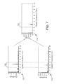
- FIG. 7 is a graphic showing three graphs and a high-level process view of frequency spectra analysis.
- Web inspection systems consist of quantitative and qualitative embodiments.
- a quantitative inspection system yields inspection information about a web property in units calibrated to a known standard, for example in engineering units. This is contrasted with qualitative inspection systems, which focus on the relative change of a web property over time.
- Qualitative inspection systems may be sufficient to recognize signal patterns indicative of particular process defects (such as chatter, die lines, mottle, and other typical non-uniformities).
- qualitative inspection systems rely on no absolute target levels or calibration procedures, they yield no reproducible metric (or set of metrics) that can be used by an operator to track whether the web process is in control, or whether changes to the process have reduced the web's level of non-uniformity from one run to the next.
- Sensors and imaging systems used for inspecting web-based products must be calibrated periodically.
- the particular calibration schedule depends on such things as the type of web being inspected, and that web's property of interest that is subject to the inspection. Additionally, environmental conditions in the operating environment (temperature, humidity, dust levels, and so forth) and production and maintenance schedules may cause inspection systems to go out of calibration, and thus necessitate calibration every few days, every few hours, or possibly even more frequently.
- Approaches to calibrating optical sensing equipment for web inspection generally fall into one or more of several categories.
- the “off-line” approach to calibrating a web inspection system involves recording the signal (optical or otherwise) produced by the web inspection system when that system is exposed to a known sample or known set of samples. In the case of an optical inspection system, this is often done by placing a series of samples into the optical path or paths of the inspection system, possibly at multiple positions. This off-line approach requires that normal web processing or production be interrupted while samples are placed into the location normally occupied by the web.
- a variation on this off-line approach is to move the web inspection system (including illumination devices) to an off-web position, generally adjacent to the line and outside the web path, where the sensing response associated with a standard sample or samples can be recorded, and thus the web inspection system calibrated. After calibration the web inspection system is restored to its web-inspection position. While the inspection system if off-line, being calibrated, web processing may proceed, but absent a second inspection system (which is costly), such processing may not be within control.
- a second approach attempts to obtain calibration data while normal web is being produced, that is, using as-produced web, albeit with as yet unknown properties.
- the inspection system records data from a first section of web whose location is either marked or otherwise known to the web handling system. When the first section of web reaches the winder, it is cut from the remainder of the web, usually as an “end-of-roll” sample, and taken to a quality control lab.
- a quality control lab Provided that accurate location information is available such to allow positions on the sample to be registered with the data stored by the inspection system when the sample passed through the inspection station, off-line quality control instruments can be used to provide calibration data for the inspection system.
- This approach is resource intensive and requires careful attention to sample registration to achieve good data, and also suffers from a substantial time lag between when the sample initially passed through the inspection station and when the calibration becomes available.
- a third approach involves some combination of the above two approaches. For example, a known sample may be placed outside the edges of the normal web path, but within the area viewed by the inspection system. This provides ongoing calibration data for the outermost sensor elements while product is still running. However, transferring calibrations to web inspection system sensor(s) over the normal web, whose properties are unknown, requires knowledge of the relation between the responses of the inner sensor elements and the responses of the outer sensor elements, and those responses must remain fixed relative to each other at all times. In another example, calibration samples are exposed to various portions of the inspection system's field-of-view, thus adding additional known offsets to the unknown properties of the web. This places some restrictions on the statistical variations of the web during calibration, and also changes the range that the inspection system may have to operate over.
- FIG. 1 shows a schematic of one embodiment of a calibration system on web handling system W 6 .
- Web handling system W 6 may be any web handling system used for manufacturing, converting, processing, or inspecting web W 1 .
- Web W 1 may be any material substantially wider than it is thick that is amenable to automated inspection.
- web W 1 may be an optical film, a battery membrane material, a paper, a type of woven material, a type of non-woven material, an abrasive, a micro-structured film, a multi-layered film, a composite film, a printed and patterned web, a foil, or sheet goods (like rolled steel).
- Web W 1 may have one or more coatings, such as wet coatings.
- web W 1 may be a web of pieces molded to form a web, or molded onto a web.
- Web W 1 moves from left to right, possibly as part of a manufacturing or converting process.
- Sensor W 2 is shown positioned up-web from web inspection system W 3 but it could also be positioned down-web from web inspection system W 3 .
- sensor W 2 could even be positioned so as to receive signals from the same web area as web inspection system W 3 .
- one or more beamsplitters could be used on signals emanating from a web area (provided both the sensor W 2 and web inspection system W 3 are based on optical signals).
- Sensor W 2 in one embodiment, is a single readout sensor configured to receive inspection signals emanating from a single lane W 4 of web W 1 , and then generate signals indicative of this response.
- Sensor W 2 may be any type of sensor—for example it may be an optical sensor (sensitive to, for example, visible light, ultraviolet, infra-red, or near infra-red, or employing terahertz imaging techniques), or a sensor configured to receive some type of electromagnetic radiation, or a sensor configured to receive acoustic waves.
- Sensor W 2 is calibrated to accurately measure a property of web W 1 in calibrated units. It is not necessary that sensor W 2 be a single point sensor, but the calibration transfer to the web inspection system described below uses a single data stream.
- a single data stream may be provided by averaging signals from several adjacent sensing elements that comprise sensor W 2 (camera pixels, capacitive sensing elements, and so forth) to obtain a single data stream.
- sensing elements There is no strict limit to the number of sensing elements that comprise sensor W 2 , however, the more elements there are in sensor W 2 , the more difficult it may become to assure they are all calibrated to the same response relative to one another.
- Web inspection system W 3 is, in one embodiment, a line-scan camera, which at least receives inspection signals associated with the same single lane W 4 as single output sensor W 2 , as well as a lane other than lane W 4 .
- a line-scan camera is relatively inexpensive and ubiquitous, but the same or similar calibration techniques and systems as described herein could accommodate other types of inspection systems.
- web inspection system W 3 may also comprise laser scanners, time-delay integration cameras, area scan cameras, other array sensors, or some combination of these systems.
- Web inspection system W 3 may receive signals from a width of web W 1 that is less than the entire width.
- Sensor W 2 is periodically calibrated against a known standard.
- the timing of sensor W 2 calibration is dependant on the propensity of the sensor to drift out of calibration and the tolerances required for a particular web processing environment.
- an optical density gauge used as sensor W 2 can be configured to measure the light transmission of a web within a particular wavelength band, but as the light source ages, its spectral output and/or power levels might change so as to affect the accuracy of the data coming from the sensor.
- the response of such a sensor could be checked periodically using a known standard or set of standards to correct for such a drift.
- the calibration of a sensor W 2 is a rather trivial matter and may be accomplished in one embodiment by swinging the single output sensor off-line to receive signals from a known standard or set of standards.
- the sensor W 2 may be calibrated using known techniques in a quality control laboratory located near the manufacturing line.
- sensor W 2 could be sent in to a manufacturer or a vendor laboratory or even a national laboratory such as the National Institute of Standards and Technology for calibration.
- web inspection system W 3 may continue inspection of the web using its previously calibrated state.
- web handling system W 6 with a plurality (2, 3, or even more) of single output sensors, such that at any given time, at least one is on-line and receiving signals from web passing in lane W 4 , such that a calibrated signal is received from at least one single output sensor while any of the other single output sensor(s) is off-line being calibrated (and vice-versa).
- Sensor W 2 in one embodiment, is configured to measure the same property as web inspection system W 3 .
- both sensor W 2 and web inspection system W 3 may in one embodiment be configured to respond to inspection signals (in this case light) in the range visible to humans.
- web inspection W 3 may be configured to measure a property different than that measured by sensor W 2 , but strongly correlated to it.
- An example of a strongly correlated property is where sensor W 2 measures thickness of the web via an ultrasonic transducer, and the web inspection system W 3 is a line scan camera sensitive to light in the human-visible spectrum.
- Another example of a web property strongly correlated with light in the human-visible spectrum is, at least in some cases, thermal conductivity, discussed above.
- Quantitative imaging system W 5 may be an application-specific or general purpose computer with memory and a central processing unit that receives input from sensor W 2 and web inspection system W 3 and analyzes the input to apply, or in some embodiments determine, a calibration model for web inspection system W 3 .
- a calibration model is one or more numerical values or algorithms that define a mathematical relationship used to convert output signals from web inspection system W 3 from raw data into calibrated units.
- the first calibration model which is the “sensor to inspection system calibration model” defines the mathematical relationship between sensor W 2 and the portion of inspection system W 3 associated with the same lane W 4 as sensor W 2 .
- the second calibration model which is the “cross-web calibration model” defines the mathematical relationship between lanes that comprise inspection system W 3 's cross-web field-of-view.
- Quantitative imaging system 5 determines the cross-web calibration model by processing data sets associated with lane W 4 (which is calibrated to point sensor W 2 via the sensor to inspection system calibration model) and data sets associated with one or more lanes other than lane W 4 , as well as data describing the cross-web signal profile of the inspection system.
- Quantitative imaging system W 5 is shown in FIG. 1 as a single system, but in alternative embodiments it may be comprised of a plurality of computers, networked together or standing alone, that execute various software algorithms in support of the calibration techniques described herein.
- FIG. 2 is a diagram showing, in one example embodiment, the functional modules that comprise quantitative imaging system W 5 .
- FIG. 2 is described with respect to a discreet set of functional modules, but a skilled artisan will understand that this description is for illustrative purposes only, and that a system having the same or similar functionality may be architected in myriad ways.
- Each of the functional modules illustrated in FIG. 2 may communicate with any of the other modules; any of the modules may be implemented in hardware or software or some combination thereof.
- User P 1 is any user of web inspection system W 5 .
- User P 1 may be a human operator responsible for quality control on web W 1 .
- User P 1 interacts with quantitative imaging system W 5 primarily through a keyboard, a mouse, and a display of some sort (none of which are shown in FIG.
- User interface module P 5 may generate a graphical user interface or a command-line type interface on a display such that user P 1 may both provide information to quantitative imaging system W 5 , and receive information from quantitative imaging system W 5 .
- user interface module P 5 generates windows on a display by calling on functionality provided by an operating system such as one marketed under the trade name “Windows” by Microsoft Corporation, Redmond, Wash. Other operating systems may be similarly used.
- User interface module P 5 in turn provides and receives data and commands from other functional modules. There may be additional interfaces (not shown in FIG. 2 ) to automated web process control or web monitoring systems.
- I/O module P 9 interfaces with sensor W 2 and web inspection system W 3 . I/O module P 9 receives data streams from sensor W 2 and web inspection system W 3 . In one example embodiment, depending on the particular implementation of quantitative imaging system W 5 , I/O module P 9 also provides command and control information to sensor W 2 and/or web inspection system W 3 . For example, elsewhere in this disclosure is described an embodiment of a cross-web transport device upon which sensor W 2 is affixed, such that sensor W 2 may move cross-web. I/O module P 9 , in such an embodiment, could provide control signals that dictate such cross-web movement. Also, I/O module P 9 may provide other information to generally control either sensor W 2 or web inspection system w 3 . Input received by I/O module P 9 may be provided to other modules directly or stored in database P 8 for subsequent analysis.
- Database P 8 is a data store implemented in a computer memory such as random access memory or a hard disk drive, or some combination thereof. It may be simply computer memory, a flat file, or a database such as that marketed by Microsoft Corporation of Redmond, Wash. under the trade name “SQL Server.” Database P 8 handles data storage needs of any of the functional modules that comprise quantitative imaging system W 5 . Data streams emanating from sensor W 2 and web inspection system W 3 may be stored in database P 8 , as well as data that comprise calibration models.
- Web inspection system control module P 7 provided command and control signals via I/O module P 9 to web inspection system W 3 .
- the particular functionality supported by web inspection system control module P 7 is dependant largely on the command and control interface provided by the particular web inspection system W 3 chosen for implementation.
- some line scan cameras that could comprise web inspection system W 3 have application programming interfaces such to support a particular set of functionality; such functionality would exist in FIG. 2 within web inspection system control module P 7 . If web inspection system W 3 has output that needs to be converted (for example, a raw voltage which needs to be converted into units), the means for conversion is implemented within web inspection system control module P 7 .
- Sensor control module P 6 is to the sensor control module P 6 what web inspection system control module P 7 is to the web inspection system W 3 , mutatis mutandis.
- Sensor-to-inspection system calibration module P 4 analyzes data from sensor W 2 (provided via I/O module P 9 and possibly stored in database P 8 ) and web inspection system W 3 and establishes the sensor to inspection system calibration model such that output from inspection system W 3 associated with the same cross-web lane as sensor W 2 is converted into the calibrated units of sensor W 2 's output. Examples of this conversion are provided below.
- Cross web calibration module P 3 determines, if necessary, and applies the calibration model provided by sensor-to-inspection system calibration module P 4 to the other lanes of web W 1 inspected by web inspection system W 3 , such that data from all lanes the comprise inspection system W 3 's field-of-view are calibrated to lane W 3 . Examples of such a calibration are provided below.
- the functional modules described in association with FIG. 2 may have further functionality that is consistent with their general nature, but was not mentioned in this disclosure. Functionality described elsewhere that is not explicitly associated with a functional module listed in FIG. 2 exists within quantitative imaging system W 5 generally. For example, the functionality that provides the alignment of signals emanating from sensor W 2 and web inspection system W 3 exists generally within quantitative imaging system W 5 .
- FIGS. 3 a and 3 b will now be described. Collectively they describe two approaches to calibrating the web inspection system, the former based on synchronizing lanes in time or down web space domains, and the later based on developing a calibration model in the frequency domain.
- FIG. 3 a is a flowchart illustrating a high-level process that may be used to calibrate the web inspection system W 3 that is shown in FIG. 1 .
- a first signal response is received from sensor W 2 , which, in this example, is located up-web from web inspection system W 3 and associated with a particular “lane” of the web line W 4 (F 1 ). In the context of FIG. 3 (a and b), this lane shall be referred to as lane X.
- Web inspection system W 3 may inspect (i.e. receive signals from) the entire width of the web (or some portion thereof), but at least inspects lane X (F 2 ). Signals from web inspection system W 3 associated with lane X are for the purposes of FIG. 3 termed the second signal response.
- the first signal response is synchronized with the second signal response (F 3 ) such that the signals from the single output sensor W 2 and the lane-X portion of web inspection system W 3 are representative of the same areas of web W 1 .
- synchronization may be accomplished by determining the time it takes for a point along web W 1 to go from single output sensor W 2 to web inspection system W 3 . This time delay may be used to define a shift which may then be applied to the respective data stream emanating from either sensor W 2 or web inspection system W 3 , thus time-synchronizing the data streams.
- one or more encoders may be used to trigger sampling of points from sensor W 2 and inspection array W 3 . The encoder(s) trigger data acquisition at fixed space intervals of the web rather than fixed time intervals, such that the two data sets are spatially synchronized.
- data analysis techniques such as cross-correlation may be used to determine the shift value necessary to time synchronize data streams emanating from sensor W 2 and web inspection system W 3 .
- data streams from sensor W 2 and the lane-X portion of web inspection system W 3 are similar such that linear cross-correlation methods are adequate to determine misalignments between the data sets.
- data streams from sensing elements adjacent to lane-X of web inspection system W 3 are compared with the data stream from sensor W 2 in order to find the best cross-web alignment for lane-X.
- the cross-web spatial location on web inspection system W 3 with the best correlation may vary slightly from the physical cross-web location of sensor W 2 due to web steering or potentially even web stretching or shrinking
- the signal outputs from several adjacent elements of web inspection system W 3 may be combined so as to better reflect the material in lane-X before the cross-correlation is carried out.
- variable transformation prior to cross-correlation in order to obtain a linear relationship between the data sets, especially in cases where a mathematical model exists for the response functions of the sensors.
- f is the vector of calibrated single output sensor data in engineering units at a particular cross-web location
- x i and g is the corresponding vector computed from appropriately weighted array sensor data at that location.
- Data sets from the sensor W 2 and the web inspection system W 3 associated with lane W 4 may be sampled discretely in time or in space using an encoder trigger acquisition at fixed sampling distances.
- the results of the sampling are stored in computer memory, such as that of quantitative imaging system W 5 , for a finite down-web section of web in order to compute the summation. It is possible to mean-center the data before performing cross-correlation, and any of a number of well-known normalization methods may also be employed.
- the two data sets in this technique have the same number of samples (which may mean the sensor and the web inspection system sampled at the same rate, or it could mean that the one of the sets was reduced or expanded using statistical extrapolation techniques).
- the sampling rates for sensor W 2 and web inspection system W 3 are identical, and the sensor and the web inspection system both resolve the same features in the property of interest.
- a combination of manual and statistical techniques may also be employed to determine the shift value to be applied to the data streams to achieve synchronization. For example, an estimate of the time it takes for a point on the web to move from sensor W 2 to web inspection system W 3 may be used to establish a window within which to use cross-correlation to get the more accurate data alignment from the peak of the cross-correlation result.
- the strength of the correlation coefficient can also be used as an indication of sensor errors, as the farther down web distance between the sensor and the web inspection system, the more web steering affects might reduce correlation.
- the first and second signal responses are next analyzed by quantitative imaging system W 5 to produce a calibration model that define(s) the relationship between the respective signal response of sensor W 2 (which will be called the first data stream for the purposes of this figure) and the area of web inspection system W 3 associated with the same lane W 4 as sensor W 2 (which will be called the second data stream for the purposes of this figure) (step F 5 ).
- a first exemplary technique described herein uses linear regression to determine the relationship, and thus correlation factor, between the first and second data streams.
- Linear regression has been found to work sufficiently well for sensors with similar response functions over a finite range of the measured property.
- Other techniques may be better suited for other combinations of sensor and web inspection system responses. For example, when dealing with wider ranges of a measured property, local linear regressions could be done at fixed intervals between data sets (for example, after the passage of a certain amount of time or a certain distance of web) or automatically as determined by the magnitude of the measured property. If a nonlinear parametric model is known to relate the data sets, one may employ nonlinear least squares to fit the parameters of the model.
- a kernel smoother may be applied to the observed curve relating aligned datasets in order to obtain a nonparametric estimate of the true relationship without recourse to any prior model.
- the goal is to find the fitting coefficients, ⁇ , that minimize the least squares error between the measured values from the calibrated sensor, f, and the values predicted by this model, ⁇ circumflex over (f) ⁇ , derived from the data from the i th element of the array sensor.
- G be the matrix whose first column is the aligned and weighted array sensor data at position x i and f be the single column vector formed from the calibrated single output sensor data, also at position x i
- G j1 ( x i ) ⁇ tilde over (g) ⁇ ( x i ,y j * )
- FIG. 3 b a flowchart is shown illustrating a second exemplary technique that can be used to establish the relationship between the first and second data streams, and thus a calibration factor (or factors) or a calibration model.
- This second exemplary technique involves computations in the frequency domain rather than the time or space domains.
- time/space series implementation (as compared with a frequency analysis) is due to the fact that not all changes in sensor and camera data sets are correlated in exactly the same way. For example, in the low frequency domain typically dominated by gradual changes in material properties and/or the background environment, the correlation models derived from time-based analysis may not be as accurate.
- transform operations could be used instead of Fourier transforms, for example wavelet transforms or a filter bank approach (an array of filters all tuned to different frequencies), or Laplace or z-transform methods known in the art. Since data from the sensor W 2 is most highly correlated with lane W 4 of pixel data from web inspection system W 3 , several processing operations are possible at this point. One could crop the image data in the cross-web direction to a single pixel column, in which case 1D transforms can be applied to both data streams. Alternatively, one could simply average together pixel columns in the lane into a single data stream, followed again by 1D transformations applied to both data streams.
- the column averaging operation above is a form of a 2D transform applied to the lane of image data. So the general case is to apply a particular 2D convolution kernel to the lane of image data, followed by transformation of the image data and selection of downweb frequency data.
- the transformed data sets will show amplitudes of variation as a function of frequency, generally referred to as frequency spectra.
- Fourier transform operations are well known to those skilled in the art, and details about how to select the data window size and carry out the operation will be known to a skilled artisan.
- An appropriate reference that describes both 1D and 2D transforms is Ronald Bracewell, Fourier Transforms and Its Applications (McGraw-Hill, 3 rd edition, 1999).
- a frequency range of interest is next selected ( FIG. 3 b , step F 13 ). This could be done manually, as, for example, by an operator with some knowledge of processing conditions that may give rise to certain frequencies of down-web anomalies (see the peaks amplitudes shown in FIG. 7 , for example, or automatically by, for example, algorithmically identifying frequency peak regions associated with the frequency spectra of the point sensor and the web inspection system. If done algorithmically, data collected from elsewhere in the process may provide information on the periodic cycle of many different potential causes (e.g. roll rotation frequencies, frequency content of tension variations, etc).
- a process controller could seek out this information, determine appropriate bands to envelop likely causes of periodic variability, and specify the frequency bands of interest to the quantitative imaging system. Within narrow frequency ranges (bands) surrounding any of these spikes, we would expect to have a time-steady (i.e. down web space steady) correlation to hold between the two data streams related to the same output web properties.
- a peak detection algorithm can be used, which for example identifies peaks using derivatives of the amplitudes and applying a threshhold value for amplitude of peaks.
- the relative amplitudes of the sensor spectra and the web inspection spectra can then be used to establish the relationship, and thus the calibration model, between the two data sets at that particular characteristic frequency range.
- Several different frequency ranges could be correlated, and the relative relationships might be different for different ranges. In fact, this is expected near the low frequency end of the spectra, since these values correspond to the constant values in the linear regression method described above.
- the two relative amplitudes from the frequency spectra allow for the establishment of a stable relationship between the two signal sets, which is the basis for the correlation model. Focusing on data within the same frequency often improves the signal-to-noise ratio of the correlation model, because it focuses in on repetitive variations and thereby greatly reduces random noise components affecting both signal streams.
- the next step is developing the correlation model ( FIG. 3 b , step F 14 ).
- the first step in developing the correlation model involves imaging the visible light transmitted through the web with each line of the image being captured in synchronization with a reference clock, if temporal analysis is desired, or a web coupled encoder in the case when spatial analysis is desired.
- the cross-web width may be subdivided into any number of sub-regions, each of which will yield a discrete measurement. Within each sub-region, a 2-D kernel is applied to the pixel data.
- the form of the kernel can be chosen to emphasize or de-emphasize certain patterns in the data, but in many cases it is sufficient to choose a kernel which is simply a weighted average corresponding to the spatial response of the point sensor.
- the simplest case of such a kernel is an average of the column data along each row to create a row-by-row signal that forms the down web data stream from the inspection system, but one skilled in the art will realize that other weighting kernals may also be useful, such as a circular Gaussian kernel for point sensors that have a circular measurement volume.
- Such an operation is effectively a low-pass filter in the cross-web direction that removes some of the random noise from such sources as analog pixel noise and granularity or porousness in the web material and provides a relatively clean down-web signal for each sub-region.
- the variables I 0 , ⁇ , and z are, respectively, the incident intensity on the back side of the web, the extinction coefficient for the material, and the thickness of the material. All of these variables are generally functions of the wavelength of light used, but we are incorporating the integral over the wavelengths of illumination into the variables listed here.
- I 1 represents one extremum of the measured intensity and I 2 represents the complementary extremum of the measure light intensity.
- the corresponding extrema in web thickness are designated as z 1 , and z 2 .
- This last equation is an example of a calibration equation.
- the extinction coefficient, alpha is known, this may be used to estimate actual caliper variability from measured variability in transmitted intensity. Conveniently, using the log of the intensity ratio excludes the reference intensity from the variability calculation; therefore, changes in backlight intensity do not impact the calibration of variability. If an independent measurement of the actual change in caliper is available, such a signal may used to estimate the extinction coefficient mentioned above.
- this reference signal will be a point displacement sensor such as a laser triangulation gauge placed at the same cross-web location as one of the sub-regions mentioned above. The intensity signal from that particular sub-region would then be compared with this reference signal to carry out the calibration method discussed in the following paragraphs.
- a measure of the reference intensity is sometimes useful if a time-invariant target for the thickness, i.e. transmitted intensity, is also desired. This can be accessed via the DC component (zero frequency) of the spectra.
- the measurement model is posed as follows where each element in the y and H vectors corresponds to a matched pair of caliper and intensity measurements:
- parameter estimation is recursively updated by the following update equation, which essentially calculates the error between the current model based estimation and the actual measurements and then multiplies it by a gain to determine how much should be added or subtracted from the estimate.
- update equation essentially calculates the error between the current model based estimation and the actual measurements and then multiplies it by a gain to determine how much should be added or subtracted from the estimate.
- the P matrix expresses how much uncertainty is in the current estimate. High uncertainty yields high gain matrices and estimate evolution proceeds aggressively.
- the R matrix expresses how much uncertainty is expected in the new measurements coming in. When uncertainty in the new measurements is high, the gain matrix is throttled back and estimate evolution is more conservative. When great confidence is placed in the new measurements, the gain of this matrix is large and estimate evolution is accelerated.
- K k P k H k T [H k P k H k T +R k ] ⁇ 1
- the method proposed here utilizes the targeted periodic caliper variability that is to be measured and, in one embodiment, takes advantage of prior knowledge about the expected frequency content.
- the periodic variability is known to fall into a limited frequency band. If this band is sufficiently narrow, the likelihood that intensity variability measured in the same range correlates to caliper variability is high.
- the resulting favorable signal-to-noise ratio greatly enhances the performance of the parameter estimation.
- the y vector and H matrix above reflect the natural variability contained in the targeted periodic signal and are populated from spectral content in the expected frequency band of the magnitude spectra from the reference and intensity signals respectively.
- the magnitude spectra for both signals are estimated using a fast fourier transform (FFT) in combination with a flat top window.
- FFT fast fourier transform
- the flat top window helps to minimize the effect of FFT bin size and location on the calibration results.
- the spectral amplitudes for thickness and intensity in each frequency bin are treated as individual measurement pairs.
- the calculation of ⁇ z is straightforward, as the magnitude at each frequency in the limited band is simply doubled.
- the intensity ratios are calculated by adding and subtracting the magnitude at each frequency in the band to the DC magnitude of the intensity signal to get I max and I min respectively and then taking the ratios of those two sets of numbers.
- the signal strength and purity may not always be at desirable levels for good estimation performance.
- the periodic signal of interest may come and go depending on current process conditions or noise may occasionally enter this frequency band for one sensor or the other.
- information from a cross-power spectrum between the intensity signal and reference signal is incorporated into the R weighing matrix.
- the ratio between the product of the standard deviation of the intensity signal, ⁇ I , and reference signal, ⁇ r , and each cross-power term is used along the diagonal of the weighting matrix. This in effect gives large authority to measurements taken when the intensity and reference signal exhibit relatively high correlation in the frequency domain especially when their amplitudes are high and well above the spectral noise floor.
- the rate of estimate evolution is most aggressive when strong, coherent signals are present and least aggressive when the signals are weak.
- An overall gain, k is included to allow the engineer to tune the overall aggressiveness of the calibration estimation.
- FIG. 4 illustrates the general setup of the estimation problem.
- the system may select a frequency band based on analysis of the frequency spectra. For example, a simple high-pass, low-pass, or band-pass selection could be used such that regions of the spectra that are likely to contain unusable data are omitted from the calculations.
- a thresholding method could also be employed where a frequency band is selected around any spectral peaks that exceed a defined amplitude threshold or regions with energy or energy density in excess of a defined energy threshold.
- the final step in calibrating the web inspection system is, optionally, for calibration factors to be applied to remaining cross-web portions of web inspection system W 3 .
- This is illustrated as step F 6 in FIG. 3 a .
- the step is not illustrated in FIG. 3 b , though the same general techniques may be used.
- This is termed cross-web calibration.
- the response of each of the sensor elements that comprise web inspection system W 3 will vary such that each one may have a slightly different output signal for the same amount of optical energy (in this example) emanating from the sample being imaged.
- the inspection system's non-uniform sensor element, or pixel, response may arise from differences in both the “background level” from pixel to pixel, that is, the signal value (although low, it is not necessarily zero) recorded when the illumination source is turned off, and the “gain” level associated with the amount of increase in output signal associated with a given unit of increase in incident optical power falling on a pixel. If one were to turn off the illumination source, one could record a background signal, and if the camera response is linear, one could take another image of a uniformly bright “white” field and characterize the response of the changes in values associated with the pixels. If the camera response is nonlinear, more than just two points would be required to characterize the response.
- inspection system W 3 images the light transmitted by a reference sample along a line illuminated by light source (for example, a line light, laser scanner, or similar device) with a line scan camera.
- I(x) the intensity distribution along the imaged section created by the illumination source
- T(x) the transmission of the sample
- R(x) the response per unit of light
- the goal is to find a(x), and b(x), such that one can invert the measured signal S(x) and recover the property T(x) of the web material.
- ⁇ (x) now contains an additional function other than just the light source and pixel response variations, we can't in general simply image the light source intensity distribution to arrive at the desired profile, although this can be adequate when the property of interest is transmission.
- T is an arbitrary time duration chosen to average out random fluctuations in measurement system noise and spatially random fluctuations in the web profile Z(x).
- the length of T may need to be adjusted according to the property being measured and the particular process, but methods for choosing the appropriate length for T based on statistical process measurements are well known in the art.
- ⁇ ( x ) k ′ ⁇ ( x ) Z ( x ) ⁇ b ( x ) where the quantities in ⁇ brackets> represent time averages.
- the profiles of ⁇ (x)> and ⁇ b(x)> tend to be relatively stable with time (that is, downweb distance) during a given run. Since values for k and b at a particular x location of the web sensor can be found essentially as often as desired using the calibration transfer method described above, the cross-web calibration problem is reduced to that of recording a relative cross-web profile ⁇ (x)> that is valid over some reasonable duration of time (>>T) to the accuracy levels required for the measurement. If the profile of ⁇ (x)> is found to drift slightly during a run, then a profile correction can be accomplished using calibrated web sensor data at only a few cross web locations as described below. A new recording for ⁇ (x)> may be required whenever there is a substantive change to the inspection system, or whenever, for example, a new product configuration changes the profile associated with ⁇ (x).
- Recording the relative cross-web calibration profile, ⁇ (x), may be accomplished in several ways.
- a single calibration sample could be scanned across the field of view of each sensor in the inspection array to map out the relative cross-web response profile.
- Z 1 the property value of this sample is in the range of interest for the web and ⁇ is only a function of x and not of Z, the exact value of Z 1 wouldn't even have to be known.
- a second example method of cross-web calibration is as follows. Before a web is in production, web inspection system W 3 could image a contiguous section of a strip of material whose profile of the desired property has been measured across an area that corresponds to the area viewed by sensor elements that comprise web inspection system W 3 , and the positions measured along the sample strip could be registered with the corresponding elements in the inspection array.
- the range of the desired property along the calibration strip does not need to be completely uniform, as long as the profile of values along the strip is known, the values lie within the operating range for a subsequent web run, and ⁇ is only a function of x and not of Z.
- the points on the strip may be physically registered with elements of the array, or cross-correlation analyses may be used to match the known profile along the strip to the measured response from the array elements.
- a third example method for cross-web calibration is to acquire an image as the web is being produced, collect the cross-web section of web corresponding to that image, and then use another calibrated sensor to measure properties across the web sample at positions corresponding to those sampled by the inspection system array elements. Several “rows” or strips across the sample could be used to reduce the impact of noise from the different sensors. Once again, this method is straightforward as long as ⁇ is only a function of x and not of Z.
- a fourth mode for performing the cross-web calibration in cases where ⁇ is only a function of x and not of Z is an iterative method that updates the cross-web calibration profile during production of the web.
- web inspection system W 3 is comprised of either several stationary web sensors W 2 of similar make fixed at different cross web locations or a movable sensor W 2 , which can be located at several different cross web locations, or a combination thereof, together with a time-average image from the inspection image.
- the number of cross web sensor locations, call it M is far less than the number of sensing locations, P, in a web inspection system W 3 that is comprised of an imaging system (such as a line scan camera).
- the web sensor locations yield only a coarse estimate of the true time-average cross-web material property profile, ⁇ Z(x)>; in general, this is adequate, because a stable ⁇ Z(x)>, often one that is relatively uniform, is the target for well-controlled manufacturing process. So, for example, time averaged data from, say, three web sensors could be used to fit up to a second order profile for ⁇ Z est (x)>.
- the fine spatial details in ⁇ (x)> and ⁇ b(x)>, related to variations in the illumination intensity profile and the sensor response and gain factors, are contained within a time-average cross-web signal profile, ⁇ S(x)>.
- the primary issue that arises in this time-average method is that of distinguishing between cross web variations in the web property ⁇ Z(x)> that are constant with time, for example streaks, and variations in ⁇ (x)> that are also constant with time, as might be caused by, for example, pieces of dirt fallen onto the illumination light source.
- This is where operations in the frequency domain can help, s the 2D kernel may help to filter out the high frequency cross web variations in the image.
- the streak wanders in and out under the sensor it is likely not a periodic wandering, so it's effect would be greatly reduced in the frequency analysis of the sensor data.
- Incorporating a repositionable sensor which can be driven to the location of the streak or to several positions along the profile to calibrate the actual web property values at those points solves this issue, again without calibrating each sensor in the array that comprises the inspection system in this example.
- New profiles akin to ⁇ Z(x)> and ⁇ (x ⁇ x)> could then be found as above, and spatial variations in the profiles could then be properly attributed to either ⁇ Z(x)> or ⁇ (x)> by comparison to the profile data prior to the displacement.
- the amount of movement required would depend upon the levels of variation in ⁇ Z(x)> and ⁇ (x)> and the signal-to-noise ratio of the time-average measurements.
- the use of a time-average signal profile obtained during normal web production is used to correct for pixel-to-pixel response variations, and the small number of cross-web calibration points used to correct for slowly varying changes in the cross-web calibration model.
- the ⁇ (x i ) vectors form a cross-web response profile, and could be used to transform the inspection system data into a calibrated, quantitative image of the cross- and down-web variations in the web properties. This mode has the advantage that it can be done while film is being produced on the line and updated periodically during a run.
- Our experience has shown that the number of cross-web calibration points, M, can be much less than the number of sensing elements in the inspection array, P, for the vast majority of cases of interest.
- FIG. 4 shows a variation on the setup of the quantitative imaging system described above.
- FIG. 4 is the same as FIG. 1 except that sensor W 2 is mounted on a cross-web transfer device WB 7 , which moves sensor W 2 to several discreet cross-web locations, thereby exposing it to several web lanes, rather than only lane W 4 .
- sensor W 2 could be automatically moved (controlled by quantitative imaging system W 5 , for example) from a cross-web position associated with lane W 4 to a second cross-web position associated with lane WB 8 . Enough samples along a down-web section of web are taken at each location so that the cross-correlation and regression method described earlier can be used at each point.
- the calibration at any given cross-web location is limited to the range of values spanned by the properties of the web over the sampled interval
- the calibration can be easily re-done by returning the calibrated sensor to the same position relative to the array sensor. For example, after some amount of time has elapsed or some amount of web has gone by, or when the measured property has changed by a predetermined amount relative to the data range spanned by the previous calibration.
- a perturbation or set of perturbations can be purposely added to the process to increase the range of the measured property sampled during the calibration.
- FIG. 5 shows one such system, where web inspection system W 3 includes two line-scan cameras.
- Sensor W 2 may be manually placed at lanes WX 1 and WX 2 , which correspond to areas within the range of the first and second line scan cameras, respectively, that comprise web inspection system W 3 .
- the sensor W 2 could be mounted to a cross-web transfer device, as discussed earlier, which moves among a plurality of lanes, possibly corresponding cross-web range of web inspection system W 3 .
- optical density is a nonlinear function of coating thickness, and it varies with wavelength.
- NIR near infrared
- a line scan camera and incandescent line light were used as the web inspection system (corresponding to web inspection system W 3 in FIG. 1 ).
- This web inspection system was used to monitor the uniformity of coating transmission over about a 6′′ cross web field of view.
- the images were normalized using a time-averaged image taken through an uncoated substrate (using a shortened exposure time to bring the signal into range) to account for variations in light source intensity profile and camera response with cross-web position.
- the spectral response was that of a typical silicon charge-coupled device with a peak response wavelength at about 650 nm and minimal response below about 400 nm and above 1000 nm. In other words, there was no attempt to make the camera view the same spectral window as the NIR sensor. The details of spectral extinction profile over the camera response range were unknown, though we knew the transmission was lower when viewed over this range than out the outset. Neglecting background light leakage in both sensors, one can show that in this case, the effect of the substrate transmission is negligible, and the following approximation holds
- OD coati ⁇ ⁇ ng ⁇ ( 1060 ) ⁇ coating ⁇ ( 1060 ) ⁇ coating ⁇ ( vis ) ⁇ OD coating ⁇ ( vis ) ( 4 ) such that for any given pixel on the camera, the OD at 1060 nm could be calculated from the visible transmission data as
- OD coating ⁇ ( 1060 , pixel ) [ - log 10 ⁇ ⁇ T ⁇ ( vis , pixel ) ⁇ - 0.036 ] ⁇ [ ⁇ coating ⁇ ( vis ) ⁇ coating ⁇ ( 1060 ) ] ( 5 )
- the 0.036 offset arises from the substrate transmission, and the last term in brackets is the calibration factor for converting the visible transmission data recorded by the camera into infrared OD units.
- Point sensors and line scan cameras were configured to monitor optical properties of birefringent polypropylene film.
- the film stretching process orients polymer molecules and creates a “fast” optical axis nominally in the downweb direction, meaning that the refractive index in this direction is slightly lower than the refractive index measured 90° from this axis, that is, the “slow” axis.
- the point sensors (corresponding to sensor W 2 in FIG. 1 ) were setup such that the incident light passed in series through a polarizer, the film, an analyzer (a 2nd polarizer crossed with the 1 st ), and onto a detector. Both the fast axis orientation and retardance sensors had similar signal response equations:
- V i A i ⁇ sin 2 ⁇ ( 2 ⁇ ( ⁇ FA - ⁇ o , i ) ) ⁇ sin 2 ⁇ ( ⁇ ⁇ i ⁇ R 0 ) + C i ( 7 )
- Sensitivity analysis showed that when the gain coefficients were adjusted to map the signals into the range [0, 10 V] for films with ⁇ FA in the range [ ⁇ 5, 5°] and R 0 in the range [45, 85 nm], the film retardance values had to be taken into account when analyzing the FA response, whereas including the true FA angle of the film (compared to assuming a FA angle of 0°) had only a minor effect on the retardance value computed from the R 0 sensor.
- Line scan cameras (corresponding to web inspection system W 3 in FIG. 1 ) were setup down-web from the sensors to view polarized line lights through the film, and analyzers were mounted on the camera lenses and crossed with the respective polarizers that served as the illumination source. Except for the units of the digitized response, the camera pixels near the center of the field-of-view received signals at near normal incidence (to the web's surface) obey similar response equations to the above. Therefore by aligning the cameras such that the point sensors were within the center of the field of view and synchronizing the camera line rate with the sampling rate of the point sensors, could use the cross correlation and regression operations described earlier to transfer the calibrated responses of the R 0 and FA point sensors to the central pixels in the respective R 0 and FA cameras. Note that this operation uses only on-line data from production film; no calibration samples were used to characterize the response of these pixels.
- FIG. 6 a is a graph showing parameter estimation results from a test web sample.
- the estimate of the unknown parameter, x 1/ ⁇ , was initialized to 25 with a very large initial uncertainty.
- the estimation did not fully converge due to the limited length of the available sample; nonetheless, it appears that convergence is likely at a value of around 30 which corresponds well with results of manual data analysis.
- the exponential decay of the uncertainty value can be seen in FIG. 6 b .
- the intensity of the backlight does not appear to significantly affect the estimation results.
- FIG. 7 shows several graphs that highlight aspects of the frequency spectra-based process earlier described.
- Groups of consecutive pixels collect light from approximately two inch wide cross-direction regions of the web. The values of the pixels in each of these groups are averaged to give an average intensity value for each region of the web at each sampling instance.
- a point sensor an opposed pair of laser triangulation displacement sensors measuring the top and bottom surfaces of the passing web, is positioned at some chosen cross-direction location. Samples of the provided web thickness signal are acquired at the same intervals of the camera line scan rate as governed by a common encoder or reference clock pulse train.
- a region of the web that is well aligned to the portion of the web measured by the point sensor is selected and the corresponding averaged intensity values constitute a sampled signal to be compared with the sampled signal acquired from the point sensor.
- a Fast Fourier Transform (FFT) is applied to both the intensity signal as well as the reference thickness signal.
- Graph 710 shows the frequency spectrum from a point sensor.
- Graph 701 shows the frequency spectrum from the web imaging system, in this case a camera.
- Frequency band 720 includes a peak of interest, clearly occurring in both graph 701 and 710 .
- the process of estimating the calibration coefficient consists of collecting two sets of several measurements: one closely related to the system involving the unknown parameter and expressed in uncalibrated units, the other coming directly from a measurement of the same subject in calibrated units.
- Each spectral component in the band of interest, 720 in FIG. 7 is treated as an individual measurement.
- the two sets of measurements just mentioned come from the same band in the intensity signal spectrum 701 and the reference thickness signal spectrum 710 respectively as indicated in the following equations.
- y [ ⁇ z i ⁇ z i+1 . . . ⁇ z i+n ] T
- the collection of reference measurements represented by y consists of the periodic change in thickness occurring at each of the n frequencies in the band of interest where i designates the first frequency falling within this band. As explained earlier, the total change in thickness at given frequency is simply calculated as twice the spectral amplitude at that frequency.
- the reference measurements are modeled to vary linearly with the unknown parameter 1/ ⁇ and that the multiplier is the natural log of the ratio between the maximum and minimum of the periodic intensity variation at each frequency in the band.
- the maximum and minimum intensities are calculated by adding and subtracting, respectively the spectral amplitude at each frequency to the mean intensity.
- the next step is to define the weighting matrix that will regulate the amount of estimate change that occurs due to each individual data point.
- the weighting matrix is also extracted from the spectral content of the two signals.
- the following matrix is used for the weighting matrix.
- the relative magnitude between the cross-power spectral components at each frequency in the band of interest to the overall cross-power of the two signals is used to determine how much the estimate is adjusted based on each individual pair of measurement data.
- the gain, k is tuned to adjust the overall responsiveness of the estimation algorithm.
- the uncertainty matrix, P is a scalar in the case, since there is only a single unknown parameter, and is set at some arbitrarily high number, 5000 for example, to allow the algorithm to quickly approach reasonable values for the calibration estimate. After the initial setting, this value is continually adjusted by the algorithm to reflect how much confidence is placed on the current estimate based on the quality of information in recent measurements. Higher values of this variable allow more liberal changes in the calibration estimate for all levels of quality in the incoming measurements.
- the deterioration matrix, Q is also scalar and is used to prevent the algorithm from becoming too static.
- This variable in effect applies upward pressure on the uncertainty matrix such that information rich measurements must occur consistently to maintain a low uncertainty; otherwise, the uncertainty will drift upwards and the algorithm will become more open to changes based on new measurements.
- This parameter is tuned in conjunction with the gain, k, contained in the R matrix by the engineer based on a qualitative assessment of the algorithm's ability to respond to changes in the calibration coefficient.
Landscapes
- Physics & Mathematics (AREA)
- General Health & Medical Sciences (AREA)
- Pathology (AREA)
- Health & Medical Sciences (AREA)
- Life Sciences & Earth Sciences (AREA)
- Chemical & Material Sciences (AREA)
- Analytical Chemistry (AREA)
- Biochemistry (AREA)
- Immunology (AREA)
- General Physics & Mathematics (AREA)
- Engineering & Computer Science (AREA)
- Textile Engineering (AREA)
- Mathematical Physics (AREA)
- Theoretical Computer Science (AREA)
- Spectroscopy & Molecular Physics (AREA)
- Investigating Materials By The Use Of Optical Means Adapted For Particular Applications (AREA)
- Investigating Or Analysing Materials By Optical Means (AREA)
- Investigating Or Analyzing Materials By The Use Of Ultrasonic Waves (AREA)
- Testing Of Devices, Machine Parts, Or Other Structures Thereof (AREA)
Priority Applications (8)
| Application Number | Priority Date | Filing Date | Title |
|---|---|---|---|
| US13/249,468 US8553228B2 (en) | 2011-09-30 | 2011-09-30 | Web inspection calibration system and related methods |
| KR1020147011665A KR20140067162A (ko) | 2011-09-30 | 2012-09-26 | 웨브 검사 교정 시스템 및 관련 방법 |
| CN201280048265.8A CN103842800B (zh) | 2011-09-30 | 2012-09-26 | 幅材检测校准系统及相关方法 |
| BR112014007577A BR112014007577A2 (pt) | 2011-09-30 | 2012-09-26 | sistema de calibração de inspeção de manta e métodos relacionados |
| EP12781502.5A EP2761270A1 (en) | 2011-09-30 | 2012-09-26 | Web inspection calibration system and related methods |
| JP2014533659A JP6122015B2 (ja) | 2011-09-30 | 2012-09-26 | ウェブ検査較正システム及び関連方法 |
| SG11201401016YA SG11201401016YA (en) | 2011-09-30 | 2012-09-26 | Web inspection calibration system and related methods |
| PCT/US2012/057167 WO2013049090A1 (en) | 2011-09-30 | 2012-09-26 | Web inspection calibration system and related methods |
Applications Claiming Priority (1)
| Application Number | Priority Date | Filing Date | Title |
|---|---|---|---|
| US13/249,468 US8553228B2 (en) | 2011-09-30 | 2011-09-30 | Web inspection calibration system and related methods |
Publications (2)
| Publication Number | Publication Date |
|---|---|
| US20130083324A1 US20130083324A1 (en) | 2013-04-04 |
| US8553228B2 true US8553228B2 (en) | 2013-10-08 |
Family
ID=47143263
Family Applications (1)
| Application Number | Title | Priority Date | Filing Date |
|---|---|---|---|
| US13/249,468 Active 2032-05-22 US8553228B2 (en) | 2011-09-30 | 2011-09-30 | Web inspection calibration system and related methods |
Country Status (8)
Cited By (3)
| Publication number | Priority date | Publication date | Assignee | Title |
|---|---|---|---|---|
| US20110203221A1 (en) * | 2008-11-18 | 2011-08-25 | Tetra Laval Holdings & Finance S.A. | Apparatus and method for detecting the position of application of a sealing strip onto a web of packaging material for food products |
| US20160072579A1 (en) * | 2013-05-01 | 2016-03-10 | The University Of Sydney | A system and a method for generating information indicative of an impairment of an optical signal |
| WO2019105670A1 (fr) * | 2017-11-30 | 2019-06-06 | Saint-Gobain Glass France | Procédé de détection de défauts de laminage dans un verre imprimé |
Families Citing this family (25)
| Publication number | Priority date | Publication date | Assignee | Title |
|---|---|---|---|---|
| DE102013108485B4 (de) * | 2013-08-06 | 2015-06-25 | Khs Gmbh | Vorrichtung und Verfahren zum Fehlertracking bei Bandmaterialien |
| US9910429B2 (en) * | 2013-09-03 | 2018-03-06 | The Procter & Gamble Company | Systems and methods for adjusting target manufacturing parameters on an absorbent product converting line |
| US9841383B2 (en) | 2013-10-31 | 2017-12-12 | 3M Innovative Properties Company | Multiscale uniformity analysis of a material |
| US9151595B1 (en) * | 2014-04-18 | 2015-10-06 | Advanced Gauging Technologies, LLC | Laser thickness gauge and method including passline angle correction |
| CN105329694B (zh) * | 2014-07-22 | 2017-10-03 | 宁波弘讯科技股份有限公司 | 一种纠偏控制方法、控制器及纠偏控制系统 |
| DE102015017470B4 (de) | 2014-08-22 | 2025-07-17 | Divergent Technologies, Inc. | Fehlererkennung für additive fertigungssysteme |
| TWI559423B (zh) * | 2014-11-04 | 2016-11-21 | 梭特科技股份有限公司 | 晶粒攝影裝置 |
| US10786948B2 (en) | 2014-11-18 | 2020-09-29 | Sigma Labs, Inc. | Multi-sensor quality inference and control for additive manufacturing processes |
| WO2016115284A1 (en) | 2015-01-13 | 2016-07-21 | Sigma Labs, Inc. | Material qualification system and methodology |
| JP6475543B2 (ja) * | 2015-03-31 | 2019-02-27 | 株式会社デンソー | 車両制御装置、及び車両制御方法 |
| US10207489B2 (en) | 2015-09-30 | 2019-02-19 | Sigma Labs, Inc. | Systems and methods for additive manufacturing operations |
| US10067069B2 (en) * | 2016-03-11 | 2018-09-04 | Smart Vision Lights | Machine vision systems incorporating polarized electromagnetic radiation emitters |
| EP3339845A3 (en) * | 2016-11-30 | 2018-09-12 | Sumitomo Chemical Company, Ltd | Defect inspection device, defect inspection method, method for producing separator roll, and separator roll |
| JP6575824B2 (ja) * | 2017-03-22 | 2019-09-18 | トヨタ自動車株式会社 | 膜厚測定方法および膜厚測定装置 |
| US11434028B2 (en) | 2017-08-04 | 2022-09-06 | Tetra Laval Holdings & Finance S.A. | Method and an apparatus for applying a sealing strip to a web of packaging material |
| US10670745B1 (en) | 2017-09-19 | 2020-06-02 | The Government of the United States as Represented by the Secretary of the United States | Statistical photo-calibration of photo-detectors for radiometry without calibrated light sources comprising an arithmetic unit to determine a gain and a bias from mean values and variance values |
| TWI794400B (zh) * | 2018-01-31 | 2023-03-01 | 美商3M新設資產公司 | 用於連續移動帶材的紅外光透射檢查 |
| CN109060806B (zh) * | 2018-08-29 | 2019-09-13 | 陈青 | 箱子底端材料类型辨识机构 |
| WO2020219076A1 (en) * | 2019-04-26 | 2020-10-29 | Hewlett-Packard Development Company, L.P. | Evaluating surfaces |
| US20220301282A1 (en) * | 2019-09-11 | 2022-09-22 | Siemens Aktiengesellschaft | Method for Analyzing Image Information Using Assigned Scalar Values |
| CN111993798B (zh) * | 2020-08-12 | 2022-04-12 | 福建实达电脑设备有限公司 | 一种页缝传感器的自动校正方法 |
| CN112800907B (zh) * | 2021-01-19 | 2024-06-07 | 广州华望半导体科技有限公司 | 鼻梁条用料情况检测方法、系统、装置和存储介质 |
| US20220356026A1 (en) * | 2021-05-06 | 2022-11-10 | Applied Materials, Inc. | Cross web tension measurement and control |
| CN117716204A (zh) * | 2021-09-27 | 2024-03-15 | 东丽株式会社 | 片状物的凹凸测定装置、片状物的凹凸测定方法 |
| CN114862843B (zh) * | 2022-06-06 | 2024-11-01 | 东北大学 | 一种基于滤波器融合的金属带材表面缺陷快速检测方法 |
Citations (15)
| Publication number | Priority date | Publication date | Assignee | Title |
|---|---|---|---|---|
| US2517330A (en) | 1949-09-07 | 1950-08-01 | Johns Manville | Apparatus for measuring the thickness of semiopaque material |
| US4247204A (en) * | 1979-02-26 | 1981-01-27 | Intec Corporation | Method and apparatus for a web edge tracking flaw detection system |
| US4570074A (en) * | 1982-09-29 | 1986-02-11 | Q-Val Incorporated | Flying spot scanner system |
| US4623524A (en) | 1985-02-08 | 1986-11-18 | Hitachi, Ltd. | Process and apparatus for recovering inert gas |
| US4914309A (en) * | 1987-05-27 | 1990-04-03 | Nippon Sheet Glass Co., Ltd. | Discriminating type flaw detector for light-transmitting plate materials |
| US5101828A (en) * | 1991-04-11 | 1992-04-07 | Rutgers, The State University Of Nj | Methods and apparatus for nonivasive monitoring of dynamic cardiac performance |
| US5506407A (en) | 1993-12-21 | 1996-04-09 | Minnesota Mining & Manufacturing Company | High resolution high speed film measuring apparatus and method |
| US6452679B1 (en) * | 1999-12-29 | 2002-09-17 | Kimberly-Clark Worldwide, Inc. | Method and apparatus for controlling the manufacturing quality of a moving web |
| US20030014147A1 (en) | 2001-07-13 | 2003-01-16 | Mario Ignagni | Data fusion of stationary array sensor and scanning sensor measurements |
| US6647140B1 (en) * | 1999-05-18 | 2003-11-11 | Bank One | Spectrum inverter apparatus and method |
| JP2004309215A (ja) | 2003-04-03 | 2004-11-04 | Mitsubishi Rayon Co Ltd | 膜厚測定装置および膜厚測定方法 |
| US20090010104A1 (en) * | 2007-07-06 | 2009-01-08 | Schlumberger Technology Corporation | Methods and systems for processing microseismic data |
| US7773226B2 (en) * | 2008-06-05 | 2010-08-10 | 3M Innovative Properties Company | Web inspection calibration system and related methods |
| US20110141269A1 (en) * | 2009-12-16 | 2011-06-16 | Stephen Michael Varga | Systems And Methods For Monitoring On-Line Webs Using Line Scan Cameras |
| US20110170762A1 (en) * | 2010-01-08 | 2011-07-14 | 3M Innovative Properties Company | Optical web-based defect detection using intrasensor uniformity correction |
Family Cites Families (3)
| Publication number | Priority date | Publication date | Assignee | Title |
|---|---|---|---|---|
| JP2004003925A (ja) * | 2002-03-29 | 2004-01-08 | Mitsubishi Paper Mills Ltd | 同時多点測定装置及び制御装置 |
| TWI427440B (zh) * | 2005-04-06 | 2014-02-21 | Kodak Graphic Comm Canada Co | 用於校正影像化規則圖案的條帶之方法與裝置 |
| US8187424B2 (en) * | 2008-08-01 | 2012-05-29 | Honeywell Asca Inc. | Time domain spectroscopy (TDS)-based method and system for obtaining coincident sheet material parameters |
-
2011
- 2011-09-30 US US13/249,468 patent/US8553228B2/en active Active
-
2012
- 2012-09-26 WO PCT/US2012/057167 patent/WO2013049090A1/en active Application Filing
- 2012-09-26 BR BR112014007577A patent/BR112014007577A2/pt not_active IP Right Cessation
- 2012-09-26 EP EP12781502.5A patent/EP2761270A1/en not_active Withdrawn
- 2012-09-26 CN CN201280048265.8A patent/CN103842800B/zh not_active Expired - Fee Related
- 2012-09-26 SG SG11201401016YA patent/SG11201401016YA/en unknown
- 2012-09-26 KR KR1020147011665A patent/KR20140067162A/ko not_active Withdrawn
- 2012-09-26 JP JP2014533659A patent/JP6122015B2/ja active Active
Patent Citations (17)
| Publication number | Priority date | Publication date | Assignee | Title |
|---|---|---|---|---|
| US2517330A (en) | 1949-09-07 | 1950-08-01 | Johns Manville | Apparatus for measuring the thickness of semiopaque material |
| US4247204A (en) * | 1979-02-26 | 1981-01-27 | Intec Corporation | Method and apparatus for a web edge tracking flaw detection system |
| US4570074A (en) * | 1982-09-29 | 1986-02-11 | Q-Val Incorporated | Flying spot scanner system |
| US4623524A (en) | 1985-02-08 | 1986-11-18 | Hitachi, Ltd. | Process and apparatus for recovering inert gas |
| US4914309A (en) * | 1987-05-27 | 1990-04-03 | Nippon Sheet Glass Co., Ltd. | Discriminating type flaw detector for light-transmitting plate materials |
| US5101828A (en) * | 1991-04-11 | 1992-04-07 | Rutgers, The State University Of Nj | Methods and apparatus for nonivasive monitoring of dynamic cardiac performance |
| US5506407A (en) | 1993-12-21 | 1996-04-09 | Minnesota Mining & Manufacturing Company | High resolution high speed film measuring apparatus and method |
| US6647140B1 (en) * | 1999-05-18 | 2003-11-11 | Bank One | Spectrum inverter apparatus and method |
| US6452679B1 (en) * | 1999-12-29 | 2002-09-17 | Kimberly-Clark Worldwide, Inc. | Method and apparatus for controlling the manufacturing quality of a moving web |
| US20030014147A1 (en) | 2001-07-13 | 2003-01-16 | Mario Ignagni | Data fusion of stationary array sensor and scanning sensor measurements |
| US6850857B2 (en) * | 2001-07-13 | 2005-02-01 | Honeywell International Inc. | Data fusion of stationary array sensor and scanning sensor measurements |
| JP2004309215A (ja) | 2003-04-03 | 2004-11-04 | Mitsubishi Rayon Co Ltd | 膜厚測定装置および膜厚測定方法 |
| US20090010104A1 (en) * | 2007-07-06 | 2009-01-08 | Schlumberger Technology Corporation | Methods and systems for processing microseismic data |
| US7773226B2 (en) * | 2008-06-05 | 2010-08-10 | 3M Innovative Properties Company | Web inspection calibration system and related methods |
| US7957000B2 (en) * | 2008-06-05 | 2011-06-07 | 3M Innovative Properties Company | Web inspection calibration system and related methods |
| US20110141269A1 (en) * | 2009-12-16 | 2011-06-16 | Stephen Michael Varga | Systems And Methods For Monitoring On-Line Webs Using Line Scan Cameras |
| US20110170762A1 (en) * | 2010-01-08 | 2011-07-14 | 3M Innovative Properties Company | Optical web-based defect detection using intrasensor uniformity correction |
Non-Patent Citations (2)
| Title |
|---|
| Craig F. Bohren and Donald R. Huffman, Absorption and Scattering Of Light By Small Particles, Wiley, 1st ed, 1983, Cover, pub. pages, Contents pp. xi-xiv. |
| International Search Report, Form PCT/ISA/210, International Application No. PCT/US2012/057167, International Filing Date: Sep. 26, 2012, 3 pages. |
Cited By (4)
| Publication number | Priority date | Publication date | Assignee | Title |
|---|---|---|---|---|
| US20110203221A1 (en) * | 2008-11-18 | 2011-08-25 | Tetra Laval Holdings & Finance S.A. | Apparatus and method for detecting the position of application of a sealing strip onto a web of packaging material for food products |
| US9170131B2 (en) * | 2008-11-18 | 2015-10-27 | Tetra Laval Holdings & Finance S.A. | Apparatus and method for detecting the position of application of a sealing strip onto a web of packaging material for food products |
| US20160072579A1 (en) * | 2013-05-01 | 2016-03-10 | The University Of Sydney | A system and a method for generating information indicative of an impairment of an optical signal |
| WO2019105670A1 (fr) * | 2017-11-30 | 2019-06-06 | Saint-Gobain Glass France | Procédé de détection de défauts de laminage dans un verre imprimé |
Also Published As
| Publication number | Publication date |
|---|---|
| EP2761270A1 (en) | 2014-08-06 |
| KR20140067162A (ko) | 2014-06-03 |
| US20130083324A1 (en) | 2013-04-04 |
| BR112014007577A2 (pt) | 2017-04-11 |
| WO2013049090A1 (en) | 2013-04-04 |
| CN103842800B (zh) | 2016-04-20 |
| CN103842800A (zh) | 2014-06-04 |
| JP2014528579A (ja) | 2014-10-27 |
| JP6122015B2 (ja) | 2017-04-26 |
| SG11201401016YA (en) | 2014-04-28 |
Similar Documents
| Publication | Publication Date | Title |
|---|---|---|
| US8553228B2 (en) | Web inspection calibration system and related methods | |
| US7957000B2 (en) | Web inspection calibration system and related methods | |
| US6381009B1 (en) | Elemental concentration measuring methods and instruments | |
| KR101342410B1 (ko) | 주기적인 회절 구조를 포함하는 층을 갖는 샘플을 측정하는시스템 | |
| US7478019B2 (en) | Multiple tool and structure analysis | |
| JP6336982B2 (ja) | その場測定のための光計測 | |
| US20060289790A1 (en) | Apparatus and method for enhanced critical dimension scatterometry | |
| US9897486B2 (en) | Method of calibrating and using a measuring apparatus that performs measurements using a spectrum of light | |
| KR102504761B1 (ko) | 박막 특성 측정 방법 | |
| US7869050B2 (en) | Systems and methods for comparative interferogram spectrometry | |
| de Sousa et al. | Evaluating the signal processing chain employed in surface plasmon resonance biosensing | |
| US7826072B1 (en) | Method for optimizing the configuration of a scatterometry measurement system | |
| US10480935B2 (en) | Thickness mapping using multispectral imaging | |
| JP2018527560A (ja) | 試料の透過度を測定するためのアセンブリ | |
| JP6784756B2 (ja) | 接合相手の表面に材料を連続させて接続する前に達成可能な接着強度を決定するためのアレンジメント | |
| US20250137920A1 (en) | Single wafer orientation tool-induced shift cleaning | |
| US7202958B1 (en) | Modeling a sample with an underlying complicated structure | |
| US20240192144A1 (en) | Substrate inspecting apparatus and operating method thereof | |
| JP3257552B2 (ja) | 表面疵検出装置 | |
| WO2025090157A1 (en) | Measurements of structures in presence of signal contaminations |
Legal Events
| Date | Code | Title | Description |
|---|---|---|---|
| AS | Assignment |
Owner name: 3M INNOVATIVE PROPERTIES COMPANY, MINNESOTA Free format text: ASSIGNMENT OF ASSIGNORS INTEREST;ASSIGNOR:WILHELM, JUSTIN W.;REEL/FRAME:026996/0262 Effective date: 20110930 |
|
| STCF | Information on status: patent grant |
Free format text: PATENTED CASE |
|
| CC | Certificate of correction | ||
| FPAY | Fee payment |
Year of fee payment: 4 |
|
| MAFP | Maintenance fee payment |
Free format text: PAYMENT OF MAINTENANCE FEE, 8TH YEAR, LARGE ENTITY (ORIGINAL EVENT CODE: M1552); ENTITY STATUS OF PATENT OWNER: LARGE ENTITY Year of fee payment: 8 |
|
| MAFP | Maintenance fee payment |
Free format text: PAYMENT OF MAINTENANCE FEE, 12TH YEAR, LARGE ENTITY (ORIGINAL EVENT CODE: M1553); ENTITY STATUS OF PATENT OWNER: LARGE ENTITY Year of fee payment: 12 |