EP3507643B1 - Verfahren zum scannen entlang einer dreidimensionalen linie und verfahren zum scannen eines bereichs von interesse durch scannen einer vielzahl von dreidimensionalen linien - Google Patents
Verfahren zum scannen entlang einer dreidimensionalen linie und verfahren zum scannen eines bereichs von interesse durch scannen einer vielzahl von dreidimensionalen linien Download PDFInfo
- Publication number
- EP3507643B1 EP3507643B1 EP17778326.3A EP17778326A EP3507643B1 EP 3507643 B1 EP3507643 B1 EP 3507643B1 EP 17778326 A EP17778326 A EP 17778326A EP 3507643 B1 EP3507643 B1 EP 3507643B1
- Authority
- EP
- European Patent Office
- Prior art keywords
- scanning
- deflectors
- obj
- axis
- drift
- Prior art date
- Legal status (The legal status is an assumption and is not a legal conclusion. Google has not performed a legal analysis and makes no representation as to the accuracy of the status listed.)
- Active
Links
- 238000000034 method Methods 0.000 title claims description 85
- 230000033001 locomotion Effects 0.000 claims description 130
- 238000005259 measurement Methods 0.000 claims description 42
- 230000003287 optical effect Effects 0.000 claims description 34
- 239000013598 vector Substances 0.000 claims description 24
- 238000001727 in vivo Methods 0.000 claims description 9
- 238000003384 imaging method Methods 0.000 description 51
- 241001465754 Metazoa Species 0.000 description 39
- 210000004556 brain Anatomy 0.000 description 32
- 230000001537 neural effect Effects 0.000 description 32
- 210000002569 neuron Anatomy 0.000 description 30
- 230000004044 response Effects 0.000 description 25
- 238000012937 correction Methods 0.000 description 24
- 238000006073 displacement reaction Methods 0.000 description 24
- 239000011159 matrix material Substances 0.000 description 23
- 230000000694 effects Effects 0.000 description 21
- 230000002123 temporal effect Effects 0.000 description 20
- 230000006870 function Effects 0.000 description 19
- 230000000392 somatic effect Effects 0.000 description 18
- 230000000638 stimulation Effects 0.000 description 15
- 210000003520 dendritic spine Anatomy 0.000 description 14
- 241000270295 Serpentes Species 0.000 description 13
- 210000001787 dendrite Anatomy 0.000 description 13
- 230000008030 elimination Effects 0.000 description 12
- 238000003379 elimination reaction Methods 0.000 description 12
- 238000004364 calculation method Methods 0.000 description 9
- 230000010354 integration Effects 0.000 description 9
- 230000001419 dependent effect Effects 0.000 description 8
- 239000006185 dispersion Substances 0.000 description 8
- 238000002474 experimental method Methods 0.000 description 8
- 230000005015 neuronal process Effects 0.000 description 8
- 230000000284 resting effect Effects 0.000 description 8
- 210000001519 tissue Anatomy 0.000 description 8
- 238000012546 transfer Methods 0.000 description 8
- 241000699670 Mus sp. Species 0.000 description 7
- 238000000386 microscopy Methods 0.000 description 7
- PCTMTFRHKVHKIS-BMFZQQSSSA-N (1s,3r,4e,6e,8e,10e,12e,14e,16e,18s,19r,20r,21s,25r,27r,30r,31r,33s,35r,37s,38r)-3-[(2r,3s,4s,5s,6r)-4-amino-3,5-dihydroxy-6-methyloxan-2-yl]oxy-19,25,27,30,31,33,35,37-octahydroxy-18,20,21-trimethyl-23-oxo-22,39-dioxabicyclo[33.3.1]nonatriaconta-4,6,8,10 Chemical compound C1C=C2C[C@@H](OS(O)(=O)=O)CC[C@]2(C)[C@@H]2[C@@H]1[C@@H]1CC[C@H]([C@H](C)CCCC(C)C)[C@@]1(C)CC2.O[C@H]1[C@@H](N)[C@H](O)[C@@H](C)O[C@H]1O[C@H]1/C=C/C=C/C=C/C=C/C=C/C=C/C=C/[C@H](C)[C@@H](O)[C@@H](C)[C@H](C)OC(=O)C[C@H](O)C[C@H](O)CC[C@@H](O)[C@H](O)C[C@H](O)C[C@](O)(C[C@H](O)[C@H]2C(O)=O)O[C@H]2C1 PCTMTFRHKVHKIS-BMFZQQSSSA-N 0.000 description 6
- 230000001133 acceleration Effects 0.000 description 6
- 230000000712 assembly Effects 0.000 description 6
- 238000000429 assembly Methods 0.000 description 6
- 230000008901 benefit Effects 0.000 description 6
- 210000005056 cell body Anatomy 0.000 description 6
- 230000008859 change Effects 0.000 description 6
- 238000001506 fluorescence spectroscopy Methods 0.000 description 6
- 230000014509 gene expression Effects 0.000 description 6
- 238000011503 in vivo imaging Methods 0.000 description 6
- 238000002372 labelling Methods 0.000 description 6
- 210000001176 projection neuron Anatomy 0.000 description 6
- 241000699666 Mus <mouse, genus> Species 0.000 description 5
- 238000010586 diagram Methods 0.000 description 5
- 238000012623 in vivo measurement Methods 0.000 description 5
- 238000005070 sampling Methods 0.000 description 5
- 230000000007 visual effect Effects 0.000 description 5
- 108091093126 WHP Posttrascriptional Response Element Proteins 0.000 description 4
- 238000004458 analytical method Methods 0.000 description 4
- 210000003050 axon Anatomy 0.000 description 4
- 230000006399 behavior Effects 0.000 description 4
- 230000003542 behavioural effect Effects 0.000 description 4
- 239000013078 crystal Substances 0.000 description 4
- 230000005284 excitation Effects 0.000 description 4
- 238000002347 injection Methods 0.000 description 4
- 239000007924 injection Substances 0.000 description 4
- 238000012986 modification Methods 0.000 description 4
- 230000004048 modification Effects 0.000 description 4
- 230000008569 process Effects 0.000 description 4
- 230000002829 reductive effect Effects 0.000 description 4
- 230000001052 transient effect Effects 0.000 description 4
- 239000013607 AAV vector Substances 0.000 description 3
- 230000036982 action potential Effects 0.000 description 3
- 210000004027 cell Anatomy 0.000 description 3
- 238000005516 engineering process Methods 0.000 description 3
- 230000006872 improvement Effects 0.000 description 3
- 239000000203 mixture Substances 0.000 description 3
- 210000002763 pyramidal cell Anatomy 0.000 description 3
- 230000001172 regenerating effect Effects 0.000 description 3
- 230000029058 respiratory gaseous exchange Effects 0.000 description 3
- 239000000243 solution Substances 0.000 description 3
- 238000001356 surgical procedure Methods 0.000 description 3
- 230000036962 time dependent Effects 0.000 description 3
- 230000009466 transformation Effects 0.000 description 3
- 238000012800 visualization Methods 0.000 description 3
- HOKKHZGPKSLGJE-GSVOUGTGSA-N N-Methyl-D-aspartic acid Chemical compound CN[C@@H](C(O)=O)CC(O)=O HOKKHZGPKSLGJE-GSVOUGTGSA-N 0.000 description 2
- 206010034972 Photosensitivity reaction Diseases 0.000 description 2
- 230000003044 adaptive effect Effects 0.000 description 2
- 230000037396 body weight Effects 0.000 description 2
- 230000001143 conditioned effect Effects 0.000 description 2
- PJMPHNIQZUBGLI-UHFFFAOYSA-N fentanyl Chemical compound C=1C=CC=CC=1N(C(=O)CC)C(CC1)CCN1CCC1=CC=CC=C1 PJMPHNIQZUBGLI-UHFFFAOYSA-N 0.000 description 2
- 229960002428 fentanyl Drugs 0.000 description 2
- 238000002073 fluorescence micrograph Methods 0.000 description 2
- 230000037433 frameshift Effects 0.000 description 2
- 238000000338 in vitro Methods 0.000 description 2
- 210000004179 neuropil Anatomy 0.000 description 2
- 208000007578 phototoxic dermatitis Diseases 0.000 description 2
- 231100000018 phototoxicity Toxicity 0.000 description 2
- 238000004445 quantitative analysis Methods 0.000 description 2
- 238000000926 separation method Methods 0.000 description 2
- 210000003625 skull Anatomy 0.000 description 2
- 230000008925 spontaneous activity Effects 0.000 description 2
- 230000002269 spontaneous effect Effects 0.000 description 2
- 230000006641 stabilisation Effects 0.000 description 2
- 230000001131 transforming effect Effects 0.000 description 2
- 210000000857 visual cortex Anatomy 0.000 description 2
- 241001655883 Adeno-associated virus - 1 Species 0.000 description 1
- 206010002091 Anaesthesia Diseases 0.000 description 1
- 238000012935 Averaging Methods 0.000 description 1
- OYPRJOBELJOOCE-UHFFFAOYSA-N Calcium Chemical compound [Ca] OYPRJOBELJOOCE-UHFFFAOYSA-N 0.000 description 1
- 241000702421 Dependoparvovirus Species 0.000 description 1
- 101000575685 Homo sapiens Synembryn-B Proteins 0.000 description 1
- DGAQECJNVWCQMB-PUAWFVPOSA-M Ilexoside XXIX Chemical compound C[C@@H]1CC[C@@]2(CC[C@@]3(C(=CC[C@H]4[C@]3(CC[C@@H]5[C@@]4(CC[C@@H](C5(C)C)OS(=O)(=O)[O-])C)C)[C@@H]2[C@]1(C)O)C)C(=O)O[C@H]6[C@@H]([C@H]([C@@H]([C@H](O6)CO)O)O)O.[Na+] DGAQECJNVWCQMB-PUAWFVPOSA-M 0.000 description 1
- 102000004310 Ion Channels Human genes 0.000 description 1
- 102100026014 Synembryn-B Human genes 0.000 description 1
- 102000055135 Vasoactive Intestinal Peptide Human genes 0.000 description 1
- 108010003205 Vasoactive Intestinal Peptide Proteins 0.000 description 1
- GXBMIBRIOWHPDT-UHFFFAOYSA-N Vasopressin Natural products N1C(=O)C(CC=2C=C(O)C=CC=2)NC(=O)C(N)CSSCC(C(=O)N2C(CCC2)C(=O)NC(CCCN=C(N)N)C(=O)NCC(N)=O)NC(=O)C(CC(N)=O)NC(=O)C(CCC(N)=O)NC(=O)C1CC1=CC=CC=C1 GXBMIBRIOWHPDT-UHFFFAOYSA-N 0.000 description 1
- 102000002852 Vasopressins Human genes 0.000 description 1
- 108010004977 Vasopressins Proteins 0.000 description 1
- 241000700605 Viruses Species 0.000 description 1
- 208000027418 Wounds and injury Diseases 0.000 description 1
- 230000037005 anaesthesia Effects 0.000 description 1
- KBZOIRJILGZLEJ-LGYYRGKSSA-N argipressin Chemical compound C([C@H]1C(=O)N[C@@H](CCC(N)=O)C(=O)N[C@@H](CC(N)=O)C(=O)N[C@@H](CSSC[C@@H](C(N[C@@H](CC=2C=CC(O)=CC=2)C(=O)N1)=O)N)C(=O)N1[C@@H](CCC1)C(=O)N[C@@H](CCCN=C(N)N)C(=O)NCC(N)=O)C1=CC=CC=C1 KBZOIRJILGZLEJ-LGYYRGKSSA-N 0.000 description 1
- 230000035045 associative learning Effects 0.000 description 1
- 230000003376 axonal effect Effects 0.000 description 1
- 230000015572 biosynthetic process Effects 0.000 description 1
- 230000017531 blood circulation Effects 0.000 description 1
- 210000004204 blood vessel Anatomy 0.000 description 1
- 230000007177 brain activity Effects 0.000 description 1
- 239000011575 calcium Substances 0.000 description 1
- 229910052791 calcium Inorganic materials 0.000 description 1
- 230000001413 cellular effect Effects 0.000 description 1
- 210000003850 cellular structure Anatomy 0.000 description 1
- 210000003710 cerebral cortex Anatomy 0.000 description 1
- 230000001427 coherent effect Effects 0.000 description 1
- 230000001054 cortical effect Effects 0.000 description 1
- 210000003618 cortical neuron Anatomy 0.000 description 1
- 239000006059 cover glass Substances 0.000 description 1
- 238000007428 craniotomy Methods 0.000 description 1
- 230000006378 damage Effects 0.000 description 1
- 238000013500 data storage Methods 0.000 description 1
- 238000013079 data visualisation Methods 0.000 description 1
- 238000001514 detection method Methods 0.000 description 1
- 201000010099 disease Diseases 0.000 description 1
- 208000037265 diseases, disorders, signs and symptoms Diseases 0.000 description 1
- 238000009826 distribution Methods 0.000 description 1
- OFBIFZUFASYYRE-UHFFFAOYSA-N flumazenil Chemical compound C1N(C)C(=O)C2=CC(F)=CC=C2N2C=NC(C(=O)OCC)=C21 OFBIFZUFASYYRE-UHFFFAOYSA-N 0.000 description 1
- 229960004381 flumazenil Drugs 0.000 description 1
- 239000007850 fluorescent dye Substances 0.000 description 1
- 238000001215 fluorescent labelling Methods 0.000 description 1
- 102000034287 fluorescent proteins Human genes 0.000 description 1
- 108091006047 fluorescent proteins Proteins 0.000 description 1
- 239000011521 glass Substances 0.000 description 1
- 230000000971 hippocampal effect Effects 0.000 description 1
- 238000005286 illumination Methods 0.000 description 1
- 230000010365 information processing Effects 0.000 description 1
- 208000014674 injury Diseases 0.000 description 1
- 230000003993 interaction Effects 0.000 description 1
- 210000001153 interneuron Anatomy 0.000 description 1
- 230000000670 limiting effect Effects 0.000 description 1
- 230000007774 longterm Effects 0.000 description 1
- 239000000463 material Substances 0.000 description 1
- 230000007246 mechanism Effects 0.000 description 1
- HRLIOXLXPOHXTA-UHFFFAOYSA-N medetomidine Chemical compound C=1C=CC(C)=C(C)C=1C(C)C1=CN=C[N]1 HRLIOXLXPOHXTA-UHFFFAOYSA-N 0.000 description 1
- 229960002140 medetomidine Drugs 0.000 description 1
- 230000001404 mediated effect Effects 0.000 description 1
- DDLIGBOFAVUZHB-UHFFFAOYSA-N midazolam Chemical compound C12=CC(Cl)=CC=C2N2C(C)=NC=C2CN=C1C1=CC=CC=C1F DDLIGBOFAVUZHB-UHFFFAOYSA-N 0.000 description 1
- 229960003793 midazolam Drugs 0.000 description 1
- 238000010172 mouse model Methods 0.000 description 1
- 210000000653 nervous system Anatomy 0.000 description 1
- 230000007230 neural mechanism Effects 0.000 description 1
- 230000007372 neural signaling Effects 0.000 description 1
- 230000004751 neurological system process Effects 0.000 description 1
- 230000008062 neuronal firing Effects 0.000 description 1
- 230000003955 neuronal function Effects 0.000 description 1
- 238000012634 optical imaging Methods 0.000 description 1
- 230000010355 oscillation Effects 0.000 description 1
- 230000036961 partial effect Effects 0.000 description 1
- 239000002245 particle Substances 0.000 description 1
- 238000002360 preparation method Methods 0.000 description 1
- 238000012545 processing Methods 0.000 description 1
- 230000001902 propagating effect Effects 0.000 description 1
- 230000010349 pulsation Effects 0.000 description 1
- 239000011734 sodium Substances 0.000 description 1
- 229910052708 sodium Inorganic materials 0.000 description 1
- 230000003595 spectral effect Effects 0.000 description 1
- 230000007480 spreading Effects 0.000 description 1
- 238000003892 spreading Methods 0.000 description 1
- 239000000725 suspension Substances 0.000 description 1
- 230000000946 synaptic effect Effects 0.000 description 1
- 230000001360 synchronised effect Effects 0.000 description 1
- 238000003786 synthesis reaction Methods 0.000 description 1
- 238000000844 transformation Methods 0.000 description 1
- 229960003726 vasopressin Drugs 0.000 description 1
- XLYOFNOQVPJJNP-UHFFFAOYSA-N water Substances O XLYOFNOQVPJJNP-UHFFFAOYSA-N 0.000 description 1
Images


Classifications
-
- G—PHYSICS
- G02—OPTICS
- G02B—OPTICAL ELEMENTS, SYSTEMS OR APPARATUS
- G02B21/00—Microscopes
- G02B21/0004—Microscopes specially adapted for specific applications
- G02B21/002—Scanning microscopes
- G02B21/0024—Confocal scanning microscopes (CSOMs) or confocal "macroscopes"; Accessories which are not restricted to use with CSOMs, e.g. sample holders
- G02B21/0036—Scanning details, e.g. scanning stages
- G02B21/0044—Scanning details, e.g. scanning stages moving apertures, e.g. Nipkow disks, rotating lens arrays
-
- G—PHYSICS
- G02—OPTICS
- G02B—OPTICAL ELEMENTS, SYSTEMS OR APPARATUS
- G02B21/00—Microscopes
- G02B21/0004—Microscopes specially adapted for specific applications
- G02B21/002—Scanning microscopes
- G02B21/0024—Confocal scanning microscopes (CSOMs) or confocal "macroscopes"; Accessories which are not restricted to use with CSOMs, e.g. sample holders
- G02B21/0036—Scanning details, e.g. scanning stages
- G02B21/0048—Scanning details, e.g. scanning stages scanning mirrors, e.g. rotating or galvanomirrors, MEMS mirrors
-
- G—PHYSICS
- G02—OPTICS
- G02B—OPTICAL ELEMENTS, SYSTEMS OR APPARATUS
- G02B21/00—Microscopes
- G02B21/0004—Microscopes specially adapted for specific applications
- G02B21/002—Scanning microscopes
- G02B21/0024—Confocal scanning microscopes (CSOMs) or confocal "macroscopes"; Accessories which are not restricted to use with CSOMs, e.g. sample holders
- G02B21/0052—Optical details of the image generation
- G02B21/0076—Optical details of the image generation arrangements using fluorescence or luminescence
-
- G—PHYSICS
- G02—OPTICS
- G02B—OPTICAL ELEMENTS, SYSTEMS OR APPARATUS
- G02B21/00—Microscopes
- G02B21/0004—Microscopes specially adapted for specific applications
- G02B21/002—Scanning microscopes
- G02B21/0024—Confocal scanning microscopes (CSOMs) or confocal "macroscopes"; Accessories which are not restricted to use with CSOMs, e.g. sample holders
- G02B21/008—Details of detection or image processing, including general computer control
-
- G—PHYSICS
- G02—OPTICS
- G02F—OPTICAL DEVICES OR ARRANGEMENTS FOR THE CONTROL OF LIGHT BY MODIFICATION OF THE OPTICAL PROPERTIES OF THE MEDIA OF THE ELEMENTS INVOLVED THEREIN; NON-LINEAR OPTICS; FREQUENCY-CHANGING OF LIGHT; OPTICAL LOGIC ELEMENTS; OPTICAL ANALOGUE/DIGITAL CONVERTERS
- G02F1/00—Devices or arrangements for the control of the intensity, colour, phase, polarisation or direction of light arriving from an independent light source, e.g. switching, gating or modulating; Non-linear optics
- G02F1/29—Devices or arrangements for the control of the intensity, colour, phase, polarisation or direction of light arriving from an independent light source, e.g. switching, gating or modulating; Non-linear optics for the control of the position or the direction of light beams, i.e. deflection
- G02F1/33—Acousto-optical deflection devices
Definitions
- the invention relates to a method for correcting motion artifacts of in vivo fluorescence measurements by scanning a region of interest with a 3D laser scanning microscope having acousto-optic deflectors for focusing a laser beam within a 3D space.
- coding and computation within neuronal networks are formed not only by the somatic integration domains, but also by highly non-linear dendritic integration centers which, in most cases, remain hidden from somatic recordings. Therefore, it would be desirable to simultaneously read out neural activity at both the population and single cell levels.
- neuronal signaling could be completely different in awake and behaving animals. Therefore novel methods are needed which can simultaneously record activity patterns of neuronal, dendritic, spinal, and axon assemblies with high spatial and temporal resolution in large scanning volumes in the brain of behaving animals.
- 3D AO scanning is capable of performing 3D random-access point scanning ( Katona G, Szalay G, Maak P, Kaszas A, Veress M, Hillier D, Chiovini B, Vizi ES, Roska B, Rozsa B (2012); Fast two-photon in vivo imaging with three-dimensional random-access scanning in large tissue volumes. Nature methods 9:201-208 ) to increase the measurement speed and signal collection efficiency by several orders of magnitude in comparison to classical raster scanning.
- pre-selected regions of interest can be precisely and rapidly targeted without wasting measurement time for unnecessary background volumes.
- 3D AO scanning increases the product of the measurement speed and the square of the signal-to-noise ratio with the ratio of the total image volume to the volume covered by the pre-selected scanning points. This ratio can be very large, about 10 6 -10 8 per ROI, compared to traditional raster scanning of the same sample volume.
- the method faces two major technical limitations: i) fluorescence data are lost or contaminated with large amplitude movement artifacts during in vivo recordings; and ii) sampling rate is limited by the large optical aperture size of AO deflectors, which must be filled by an acoustic wave to address a given scanning point.
- the first technical limitation occurs because the actual location of the recorded ROIs is continuously changing during in vivo measurements due to tissue movement caused by heartbeats, blood flow in nearby vessels, respiration, and physical motion. This results in fluorescence artifacts because of the spatial inhomogeneity in the baseline fluorescence signal of all kinds of fluorescent labelling.
- US2015085346 A1 discloses a method for scanning along a continuous scanning trajectory with a scanner system comprising two pairs of acousto-optical deflectors.
- WO2010055362 A2 discloses ribbon like scanning trajectories for imaging dendrites.
- the present invention provides a novel method, 3D drift AO microscopy, in which, instead of keeping the same scanning position, the excitation spot is allowed to drift in any direction with any desired speed in 3D space while continuously recording fluorescence data with no limitation in sampling rate.
- non-linear chirps are used in the AO deflectors with parabolic frequency profiles.
- the partial drift compensation realized with these parabolic frequency profiles allows the directed and continuous movement of the focal spot in arbitrary directions and with arbitrary velocities determined by the temporal shape of the chirped acoustic signals.
- the fluorescence collection is uninterrupted, lifting the pixel dwell time limitation of the previously used point scanning.
- pre-selected individual scanning points can be extended to small 3D lines, surfaces, or volume elements to cover not only the pre-selected ROIs but also the neighbouring background areas or volume elements.
- Area scanning used in these methods allows motion artifact correction on a fine spatial scale and, hence, the in vivo measurement of fine structures in behaving animals. Therefore, fluorescence information can be preserved from the pre-selected ROIs during 3D measurements even in the brain of behaving animals, while maintaining the 10-1000 Hz sampling rate necessary to resolve neural activity at the individual ROIs. It can be demonstrated that these scanning methods can decrease the amplitude of motion artifacts by over an order of magnitude and therefore enable the fast functional measurement of neuronal somata and fine neuronal processes, such as dendritic spines and dendrites, even in moving, behaving animals in a z-scanning range of more than 650 ⁇ m in 3D.
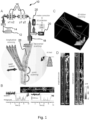
- FIG. 1A An exemplary laser scanning acousto-optic (AO) microscope 10 is illustrated in Fig. 1A which can be used to perform the method according to the invention.
- the AO microscope 10 comprises a laser source 12 providing a laser beam 14, acousto-optic deflectors 16 and an objective 18 for focusing the laser beam 14 on a sample, and one or more detectors 20 for detecting back scattered light and/or fluorescent light emitted by the sample.
- Other arrangement of the AO deflectors 16 is also possible as known in the art. Further optical elements (e.g.
- mirrors, beam splitters, Faraday isolator, dispersion compensation module, laser beam stabilisation module, beam expander, angular dispersion compensation module, etc. may be provided for guiding the laser beam 14 to the AO deflectors 16 and the objective 18, and for guiding the back scattered and/or the emitted fluorescent light to the detectors 20 as is known in the art (see e.g. Katona et al. "Fast two-photon in vivo imaging with three-dimensional random-access scanning in large tissue volumes", Nature methods 9:201-208; 2012 ). Naturally, a laser scanning microscope 10 with a different structure may also be used.
- the laser source 12 used for two-photon excitation may be a femtosecond pulse laser, e.g. a mode-locked Ti:S laser, which produces the laser beam 14.
- the laser beam 14 consists of discrete laser pulses, which pulses have femtosecond pulse width and a repetition frequency in the MHz range.
- a Faraday isolator is located in the optical path of the laser beam 14, which prevents the reflection of the laser beam, thereby aiding smoother output performance.
- the laser beam 14 After passing through the Faraday isolator, the laser beam 14 preferably passes into a dispersion compensation module, in which a pre-dispersion compensation is performed with prisms in a known way. After this, the laser beam 14 preferably passes through a beam stabilisation module, and a beam expander before reaching the AO deflectors 16.
- the laser beam 14 deflected by the AO deflectors 16 preferably passes through an angular dispersion compensation module for compensating angular dispersion of the beam 14 as is known in the art.
- the objective 18 focuses the laser beam 14 onto a sample 26 placed after the objective 18.
- a beam splitter is placed between the angular dispersion compensation module and the objective 18, which transmits a part of the laser beam 14 reflected from a sample 26 and or emitted by the sample 26 and collected by the objective 18 to the photomultiplier (PMT) detectors 20, as is known in the art.
- PMT photomultiplier
- scanning points are extended to 3D lines and/or surfaces and/or volume elements in order to substantially increase the signal to noise ratio, which allows for performing measurements in vivo, e.g. in a moving brain.
- the 3D drift AO scanning according to the invention allows not only for scanning individual points, but also for scanning along any segments of any 3D lines situated in any location in the entire scanning volume. Therefore, any folded surface (or volume) elements can be generated, for example from transversal or longitudinal lines as illustrated in Fig. 1A . In this way, fluorescence information can be continuously collected when scanning the entire 3D line in the same short period of time ( ⁇ 20 ⁇ s) as required for single-point scanning in the point-by-point scanning mode. Data acquisition rate is limited only by the maximal sampling rate of the PMT detectors 20.
- the first step is to select guiding points along a region of interest (e.g. a dendritic segment or any other cellular structure).
- a region of interest e.g. a dendritic segment or any other cellular structure.
- the second step is to fit a 3D trajectory to these guiding points using e.g. piecewise cubic Hermite interpolation.
- Two preferred strategies to form ribbons along the selected 3D trajectory are to generate drifts (short scans during which the focus spot moves continuously) either parallel to the trajectory (longitudinal drifts), or orthogonal to the trajectory (transverse drifts) as illustrated in Fig. 1A .
- drifts short scans during which the focus spot moves continuously
- Fig. 1A it is preferred to maximize how parallel these surface elements lie to the plane of brain motion or to the nominal focal plane of the objective.
- the basic idea behind the latter is that the point spread function is elongated along the z axis: fluorescence measurements are therefore less sensitive to motion along the z axis. Therefore, it is also possible to follow this second strategy and generate multiple x-y frames for neuronal network and neuropil measurements (see below).
- Example 1 3D ribbon scanning to compensate in vivo motion artifacts
- FIG. 1C shows a 3D image of a dendritic segment of a selected GCaMP6f-labelled neuron. Cre-dependent GCaMP6f-expressing AAV vectors were used to induce sparse labelling.
- a 3D ribbon (indicated with dashed lines) was selected for fast 3D drift AO scanning within the cuboid
- 3D recorded data were projected into 2D as a function of perpendicular and transversal distances along the surface of the ribbon. Note that, in this way, the dendritic segment was straightened to a frame ( Figure 1D ) to record its activity in 2D movies. This projection also allowed the use of an adapted version of prior art methods developed for motion artifact elimination in 2D scanning (see Greenberg DS, Kerr JN (2009) Automated correction of fast motion artifacts for two-photon imaging of awake animals. Journal of neuroscience methods 176:1 -15 .).
- Fig. 1B illustrates exemplified dendritic and spine transients which were recorded using 3D random-access point scanning during motion (light) and rest (dark) from one dendritic and one spine region of interest (ROI) indicated with white triangles in the inset. Note that fluorescence information can reach the background level in a running period, indicating that single points are not sufficient to monitor activity in moving, behaving animals.
- Figs 2A - 2H demonstrate the quantitative analysis of the motion artifact elimination capability of 3D drift AO scanning.
- FIG. 2A shows exemplified transient of brain displacement projected on the x axis from a 225 s measurement period when the mouse was running (light) or resting (dark) in a linear maze. Movement periods of the head-restrained mice were detected by using the optical encoder of the virtual reality system.
- Displacement data were separated into two intervals according to the recorded locomotion information (running in light colour and resting in dark colour) and a normalized amplitude histogram of brain motion was calculated for the two periods (see Fig. 2B ). Inset shows average and average peak-to-peak displacements in the resting and running periods.
- the inset shows a dendritic segment example. ⁇ F/F was averaged along a dashed line and then the line was shifted and averaging was repeated to calculate ⁇ F/F(x).
- Brain motion can induce fluorescence artifacts, because there is a spatial inhomogeneity in baseline fluorescence and also in the relative fluorescence signals ( Figure 2C ).
- the amplitude of motion-generated fluorescence transients can be calculated by substituting the average peak-to-peak motion error into the histogram of the relative fluorescence change ( Figure 2C ).
- FIG. 2D On the left of Fig. 2D an image of a soma of a GCaMP6f-labelled neuron can be seen. Points and dashed arrows indicate scanning points and scanning lines, respectively. On the right, Fig. 2D shows normalized increase in signal-to-noise ratio calculated for resting (dark) and running (light) periods in awake animals when scanning points were extended to scanning lines in somatic recordings, as shown on the left. Signal-to-noise ratio with point-by-point scanning is indicated with dashed line.
- Fig. 2E demonstrates similar calculations as in Fig. D, but for dendritic recordings.
- Signal-to-nose ratio of point-by-point scanning of dendritic spines was compared to 3D ribbon-scanning during resting (dark) and running (light) periods. Note the more than 10-fold improvement when using 3D ribbon scanning.
- Fig. 2G shows further examples for motion-artifact correction.
- a single frame can be seen from the movie recorded with 3D ribbon scanning from an awake mouse.
- exemplified Ca 2+ transients can be seen that are derived from the recorded movie frames from the color-coded regions.
- the signal-to-noise ratio of the transients improved when they were derived following motion-artifact correction with subpixel resolution.
- Example 2 Recording of spiny dendritic segments with multiple 3D ribbon scanning
- dendritic segments form non-linear computational subunits which also interact with each other, for example through local regenerative activities generated by non-linear voltage-gated ion channels.
- the direct result of local dendritic computational events remains hidden in somatic recordings. Therefore, to understand computation in neuronal networks we also need novel methods for the simultaneous measurement of multiple spiny dendritic segments.
- the top image is a single frame from the movie recorded at 18.4 Hz.
- the inset is an enlarged view of dendritic spines showing the preserved two-photon resolution.
- numbers indicate 132 ROIs: dendritic segments and spines selected from the video. Note that, in this way, all the dendritic segments are straightened and visualized in parallel. In this way we are able to transform and visualize 3D functional data in real-time as a standard video movie.
- the 2D projection used here allows fast motion artifact elimination and simplifies data storage, data visualization, and manual ROI selection.
- each ribbon can be oriented differently in the 3D space, the local coordinate system of measurements varies as a function of distance along a given ribbon, and also between ribbons covering different dendritic segments. Therefore, brain motion generates artifacts with different relative directions at each ribbon, so the 2D movement correction methods used previously cannot be used for the flattened 2D movie generated from ribbons.
- the recordings of each dendritic region into short segments. Then the displacement of each 3D ribbon segment was calculated by cross-correlation, using the brightest image as a reference. Knowing the original 3D orientation of each segment, the displacement vector for each ribbon segment could be calculated. Then we calculated the median of these displacement vectors to estimate the net displacement of the recorded dendritic tree.
- Example 3 Multi-layer, multi-frame imaging of neuronal networks: chessboard scanning.
- Random-access point scanning is a fast method which provides good signal-to-noise ratio for population imaging in in vitro measurements and in anesthetized mouse models; however, point scanning generates large motion artifacts during recording in awake, behaving animals for two reasons.
- First, the amplitude of motion artifacts is at the level of the diameter of the soma.
- Second, baseline and relative fluorescence is not homogeneous in space, especially when GECIs are used for labelling ( Figure 2C ).
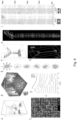
- Fig. 4B is a schematic perspective view of the selected scanning regions. Neurons from a mouse in V1 region were labelled with GCaMP6f sensor. Neuronal somata and surrounding background areas (small horizontal frames) were selected according to a z-stack taken at the beginning of the measurements. Scalebars in Fig. 4B are 50 ⁇ m.
- FIG. 4C selected frames are "transformed” into a 2D "chessboard", where the "squares" correspond to single somata. Therefore, the activity can be recorded as a 2D movie.
- the image shown in Fig. 4C is a single frame from the video recording of 136 somata during visual stimulation.
- Fig. 4D shows representative somatic Ca 2+ responses derived from the colour-coded regions in Fig. 4C following motion-artifact compensation.
- Fig. 4E shows raster plot of average Ca 2+ responses induced with moving grating stimulation into eight different directions from the colour coded neurons shown in Fig. 4C .
- Multi-layer, multi-frame scanning combines the advantage of low phototoxicity of low-power temporal oversampling (LOTOS) with the special flexibility of the 3D scanning capability of AO microscopy by allowing simultaneous imaging along multiple small frames placed in arbitrary locations in the scanning volume with speeds greater than resonant scanning.
- LOTOS low-power temporal oversampling
- Multi-layer, multi-frame scanning can also be used to measure neuronal processes ( Figure 4F ).
- Fig. 4F shows the schematic of the measurement. Multiple frames in different size and at any position in the scanning volume can be used to capture activities. Because the total z-scanning range with GECIs was extended to over 650 ⁇ m, we can, for example, simultaneously image apical and basal dendritic arbors of layer II/III or V neurons, or follow the activity of dendritic trees in this z-scanning range. To demonstrate the large dendritic imaging range, we selected a GCaMP6f-labelled layer V neuron from a sparsely labelled V1 network ( Figure 4G ). Fig.
- FIG. 4H shows the x-z projection of the neuron shown in Fig. 4G .
- Visual stimulation-induced dendritic and somatic Ca 2+ responses were simultaneously imaged at 30 Hz in multiple frames situated at 41 different depth levels in over a 500 ⁇ m z range in an awake animal ( Figures 4H ).
- Colour-coded frames indicated in Fig. 4G show the position of the simultaneously imaged squares. Motion artifacts were eliminated from frames as above by subtracting the time-dependent net displacement vector providing a motion correction with subpixel resolution.
- FIG. 4I shows the Ca 2+ transients for each ROI (see Fig. 4I ). Transients were induced by moving gratings stimulation in time periods shown in gray.
- the multi-layer, multi-frame scanning method is not limited to a single dendrite of a single neuron, but rather we can simultaneously image many neurons with their dendritic (or axonal) arbor.
- Fig. 5A shows a 3D view of a layer II/III neuron labelled with the GCaMP6f sensor. Rectangles indicate four simultaneously imaged layers (ROI 1-4). Numbers indicate distances from the pia matter. Neurons were labelled in the V1 region using sparse labelling. Somata and neuronal processes of the three other GCamP6f labelled neurons situated in the same scanning volume were removed from the z-stack for clarity.
- FIG. 5B shows average baseline fluorescence in the four simultaneously measured layers shown in Fig. 5A . Numbers in the upper right corner indicates imaging depth from the pia matter.
- Fig. 5C representative Ca 2+ transients were derived from the numbered yellow sub-regions shown in Fig. 5B following motion artifact elimination. Responses were induced by moving grating stimulation into three different directions at the temporal intervals indicated with gray shadows.
- Fig. 5D the averaged baseline fluorescence images from Fig. 5B are shown on gray scale and were overlaid with the color-coded relative Ca 2+ changes ( ⁇ F/F).
- 3D ribbons selected for 3D scanning can be extended to 3D volume elements (3D "snakes”) to completely involve dendritic spines, parent dendrites, and the neighbouring background volume to fully preserve fluorescence information during brain movement in awake, behaving animals.
- Fig. 6B is a z projection of a spiny dendritic segment of a GCaMP6f-labelled layer II/III neuron selected from a sparsely labelled V1 region of the cortex for snake scanning ( Figure 6B ). Selected dendritic segment is shown at an enlarged scale. According to the z-stack taken at the beginning, we selected guiding points, interpolated a 3D trajectory, and generated a 3D ribbon which covered the whole segment as described above.
- Fig. 6D shows the same dendritic segment as in Fig. 6C , but the 3D volume is shown as x-y and z-y plane projections.
- Representative spontaneous Ca 2+ responses were derived from the coded sub-volume elements correspond to dendritic spines and two dendritic regions.
- Transients were derived from the sub-volume elements following 3D motion correction at subpixel resolution.
- Ca 2+ transients could be calculated from different sub-volumes ( Figure 6D ). Note that, due to the preserved good spatial resolution, we can clearly separate each spine from each other and from the mother dendrite in moving animals. Therefore, we can simultaneously record and separate transients from spines even when they are located in the hidden and overlapping positions which are required to precisely understand dendritic computation ( Figure 6D ).
- Fig. 6E shows a schematic perspective illustration of the 3D multi-cube scanning.
- Fig. 6F shows volume-rendered image of 10 representative cubes selecting individual neuronal somata for simultaneous 3D volume imaging.
- 50 somata can be recorded with 50 Hz when using cubes made of 50 ⁇ 10 ⁇ 5 voxels.
- ROIs can be ordered next to each other for visualization ( Figure 6F ) .
- Ca 2+ transients were derived from the 10 cubes shown in Fig. 6F .
- We found that the use of volume scanning reduced the amplitude of motion artifacts in Ca 2+ transient by 19.28 ⁇ 4.19-fold during large-amplitude movements in behaving animals.
- FIG. 7A shows a schematic perspective illustration of multi-3D line scanning. Each scanning line is associated with one spine. In this case, we can extend each point of 3D random-access point scanning to only multiple short 3D lines instead of multiple surface and volume elements ( Figure 7A ).
- first step we selected points from the z-stack.
- second step we recorded brain motion to calculate the average trajectory of motion.
- FIG. 7B amplitude of brain motion was recorded in 3D using three perpendicular imaging planes and a bright fluorescence object as in Fig. 2A . Average motion direction is shown in the z projection image of the motion trajectory.
- Fig. 7C shows z projection of a layer 2/3 pyramidal cell, labelled with GCaMP6f. We simultaneously detected the activity of 169 spines along the 3D lines ( Figures 7C and E ).
- White lines indicate the scanning line running through the 164 pre-selected spines. All scanning lines were set to be parallel to the average motion shown in Fig. 7B . The corresponding 3D Ca 2+ responses recorded simultaneously along the 164 spines. In Fig. 7D a single raw Ca 2+ response is recorded along 14 spines using Multi-3D line scanning. Note the movement artifacts in the raw fluorescence.
- Fig. 7E shows exemplified spine Ca 2+ transients induced by moving grating stimulation in four different directions indicated at the bottom were recorded using point-by-point scanning (left) and multi-3D line scanning (right).
- Fig. 7F shows selected Ca 2+ transients measured using point scanning (left) and multi-3D line scanning (right). If we switched back from the multi-3D line scanning mode to the classical 3D point-by-point scanning mode, oscillations induced by heartbeat, breathing, and physical motion appeared immediately in transients ( Figure 7F ). These data showed an improvement in the signal-to-noise ratio when multi-3D line scanning was used. In cases when the amplitude of the movement is small and mostly restricted to a 3D trajectory, we can effectively use multi-3D line scanning to rapidly record over 160 dendritic spines in behaving animals.
- 3D drift AO scanning with which we have generated six novel scanning methods: 3D ribbon scanning; chessboard scanning; multi-layer, multi-frame imaging; snake scanning; multi-cube scanning; and multi-3D line scanning shown in Fig. 8 . Points, lines, surface and volume elements illustrate the ROIs selected for measurements.
- Each of these scanning methods is optimal for a different neurobiological aim and can be used alone or in any combination for the 3D imaging of moving samples in large scanning volumes.
- Our method allows, for the first time, high-resolution 3D measurements of neuronal networks at the level of tiny neuronal processes, such as spiny dendritic segments, in awake, behaving animals, even under conditions when large-amplitude motion artifacts are generated by physical movement.
- the above described novel laser scanning methods for 3D imaging using drift AO scanning methods have different application fields based on how they are suited to different brain structures and measurement speed.
- the fastest method is multi-3D line scanning, which is as fast as random access point-by-point scanning (up to 1000 ROIs with 53 kHz per ROI) and can be used to measure spines or somata ( Figure 8 ) .
- multi-layer, multi-frame imaging, chessboard scanning, and 3D ribbon scanning can measure up to 500 ROIs with 5.3 kHz per ROI along long neuronal processes and somata.
- the two volume scanning methods allow measurement of up to 50-100 volume elements up to about 1.3 kHz per volume element, and are ideal for measuring somata and spiny dendritic segments, respectively.
- the two volume scanning methods provide the best noise elimination capability because fluorescence information can be maximally preserved.
- mice were anesthetized with a mixture of midazolam, fentanyl, and medetomidine (5 mg, 0.05 mg and 0.5 mg/kg body weight, respectively); the V1 region of the visual cortex was localized by intrinsic imaging (on average 0.5 mm anterior and 1.5 mm lateral to the lambda structure); a round craniotomy was made over the V1 using a dental drill, and was fully covered with a double cover glass, as described previously (see Goldey GJ, Roumis DK, Glickfeld LL, Kerlin AM, Reid RC, Bonin V, Schafer DP, Andermann ML (2014); Removable cranial windows for long-term imaging in awake mice.
- mice were awakened from the fentanyl anesthesia with a mixture of nexodal, revetor, and flumazenil (1.2 mg, 2.5 mg, and 2.5 mg/kg body weight, respectively) and kept under calm and temperature-controlled conditions for 2-12 minutes before the experiment. Before the imaging sessions, the mice were kept head-restrained in dark under the 3D microscope for at least 1 hour to accommodate to the setup. In some of the animals, a second or third imaging session was carried out after 24 or 48 hours, respectively.
- the V1 region was localized with intrinsic imaging, briefly: the skin was opened and the skull over the right hemisphere of the cortex was cleared.
- the intrinsic signal was recorded using the same visual stimulation protocol we used later during the two-photon imaging session.
- the injection procedure was performed as described previously ( Chen TW, Wardill TJ, Sun Y, Pulver SR, Renninger SL, Baohan A, Schreiter ER, Kerr RA, Orger MB, Jayaraman V, Looger LL, Svoboda K, Kim DS (2013); Ultrasensitive fluorescent proteins for imaging neuronal activity. Nature 499:295-300 ) with some modifications.
- a 0.5 mm hole was opened in the skull with the tip of a dental drill over the V1 cortical region (centered 1.5 mm lateral and 1.5 mm posterior to the bregma).
- the glass micro-pipette (tip diameter ⁇ 10 ⁇ m) used for the injections was back-filled with 0.5 ml vector solution ( ⁇ 6 ⁇ 10 13 particles/ml) then injected slowly (20 nl/s for first 50 nl, and with 2 nl/s for the remaining quantity) into the cortex, at a depth of 400 ⁇ m under the pia.
- AAV9.Syn.GCaMP6s.WPRE.SV40 or AAV9.Syn.Flex.GCaMP6f.WPRE.SV40 both viruses were from Penn Vector Core, Philadelphia, PA.
- For sparse labeling we injected the 1:1 mixture of AAV9.Syn.Flex.GCaMP6f.WPRE.SV40 and AAV1.hSyn.Cre.WPRE.hGH diluted 10,000 times. The cranial window was implanted 2 weeks after the injection over the injection site, as described in the surgical procedure section.
- 3D scanning methods may also provide the key to understanding synchronization processes mediated by neuronal circuitry locally and on a larger scale: these are thought to be important in the integrative functions of the nervous system or in different diseases. Importantly, these complex functional questions can be addressed with our methods at the cellular and sub-cellular level, and simultaneously at multiple spiny (or aspiny) dendritic segments, and at the neuronal network level in behaving animals.
- the maximal, over 1000 ⁇ m z scanning range of AO microscopy which is limited during in vivo measurements with GECIs to about 650 ⁇ m by the maximal available power of the currently available lasers, already permitted simultaneous measurement of apical and basal dendritic segments of layer II/III neurons and dendritic segments of a layer V neurons in an over 500 ⁇ m range.
- the main advantage of the multi-3D ribbon and snake scanning methods is that any ROI can be flexibly selected, shifted, tilted, and aligned to the ROIs without any constraints; therefore, complex dendritic integration processes can be recorded in a spatially and temporally precise manner.
- Fig. 9 in our paraxial model we use two lenses with F 1 and F 2 focal distances at a distance of F 1 +F 2 (afocal projection) to image the two AO deflectors (AOD x 1 and AOD x 2 ) to the objective.
- Fobjective is the focal length of the objective
- z x defines the distance of the focal spot from the objective lens along the z-axis
- t 1 and t 2 are distances between the AO deflector and the first lens of the afocal projection, and between the second lens and the objective, respectively.
- the geometrical optical description of the optical system can be performed by the ABCD matrix technique.
- the deflectors deflecting along x and y directions are also linked by optical systems that can be also modelled paraxially using the ABCD matrix system.
- optical systems that can be also modelled paraxially using the ABCD matrix system.
- small letters a b c d.
- x 2 ⁇ 2 a b c d ⁇ x 1 ⁇ 1
- ⁇ 2 ′ ⁇ 2 + K ⁇ f 2
- x 0 t A ⁇ a ⁇ x 1 + b ⁇ K ⁇ f 1 x 1 t + B ⁇ c ⁇ x 1 + d ⁇ K ⁇ f 1 x 1 t + K ⁇ f 2 a ⁇ x 1 + b ⁇ K ⁇ f 1 x 1 t , t
- x 0 t A ⁇ a + B ⁇ c ⁇ x 1 + A ⁇ b ⁇ K + B ⁇ d ⁇ K ) ⁇ f 1 x 1 t + B ⁇ K ⁇ f 2 a ⁇ x 1 + b ⁇ K ⁇ f 1 x 1 t , t
- x 0 t A ⁇ a + B ⁇ c ⁇ x 1 + A ⁇ b ⁇ K + B ⁇ d ⁇ K ⁇ f 1 0,0 + a x1 t ⁇ t ⁇ D 2 ⁇ v a ⁇ x 1 v a + B ⁇ K ⁇ f 2 0 ,0 + a x2 t ⁇ t ⁇ D 2 ⁇ v a ⁇ a ⁇ x 1 + b ⁇ K ⁇ f 1 0,0 + a x1 t ⁇ t ⁇ D 2 ⁇ v a ⁇ x 1 v a v a we get the form of the equation that depends only on x 1 and t.
- the linear x 1 term coefficient A ⁇ a + B ⁇ c ⁇ A ⁇ K ⁇ b ⁇ a x1 t + K ⁇ B ⁇ a ⁇ a x2 t + K ⁇ B ⁇ a x1 t ⁇ d v a + a x1 t ⁇ a x2 t ⁇ b ⁇ B ⁇ K 2 v a 2
- a x1 and a x2 parameters must depend on t in this case.
- a x 2 t c x 2 + b x 2 ⁇ t ⁇ D 2 ⁇ v a ⁇ a ⁇ x 1 + b ⁇ K ⁇ f 1 x 1 t v a
- x 0 depends only on x 1 and t.
- x 1 dependent terms have to vanish.
- x 1 dependent terms There are four terms, that have linear, quadratic, cubic and fourth power dependence, and all are depending on t, in the general case.
- the general equation 22 can be applied to different optical setups using the particular applicable variables for the matrix elements.
- all deflectors are optically linked by telescopes composed by different focal length lenses.
- Equations 23-26 can be applied to get the appropriate matrix elements to describe equation 22. If the deflectors deflecting along the x and y axes are positioned alternately, e.g. one x is followed by one y, the telescopes linking the two x direction (x 1 and x 2 ) and y direction (y 1 and y 2 ) deflectors are described by the multiplication of the matrices describing the x 1 and x 2 and y 1 and y 2 deflectors respectively.
- the optical transfer between the last deflector and the targeted sample plane will be different for the deflectors deflecting along x and y.
- the optical system linking the last x deflector to the sample plane contains also the telescope between x 2 and y 2 deflectors made of the lenses with focal lengths f 3 ' and f 4 ' , the distance between deflector x 2 and lens f 3 ' being d 3 ', that between lenses f 3 ' and f 4 ' being f 3'+ f 4 ', and that between f 4 ' and deflector y 2 being d 4 '.
- a y B y C y D y ⁇ F 2 F obj F 1 F obj ⁇ z y , F 1 + F 2 ⁇ F 1 + F 2 z y F obj ⁇ F 2 t 1 F 1 ⁇ F 1 t 2 F 2 ⁇ F 1 z y F 2 + z y F obj F 2 t 1 F 1 + F 1 t 2 F 2 F 1 F obj , F 2 t 1 F 1 F obj ⁇ F 1 F 2 F obj F 2 + F obj ⁇ t 2 ⁇ F 2 F obj
- the values a,b,c,d and A,B, C, D of the matrices can be used in equations like Equation 22 to determine temporal variations of the x 0 and y 0 coordinates of the focal.
- the deflectors are placed in the order x 1 - x 2 - y 1 - y 2 , without intermediate telescopes or lenses.
- the distances between the deflectors are d 1 , d 2 and d 3 respectively, starting form deflector x 1 .
- the thicknesses of the deflectors cannot be neglected relative to the distances between them, their optical thicknesses (refractive index times physical thickness) are denoted by tx 1 , tx 2 , ty 1 , ty 2 , respectively.
- the optical system between the deflector y 2 and the sample plane is the same as in the previously analyzed microscope, formed by three lenses of focal lengths F 1 , F 2 and F obj , placed at the same distances as before.
- a x B x C x D x 1 z x 0 1 1 0 ⁇ 1 F obj 1 1 t 2 0 1 1 0 ⁇ 1 F 2 1 1 F 1 + F 2 0 1 1 0 ⁇ 1 F 1 1 1 t 1 0 1 1 ty 2 0 1 1 d 3 0 1 1 ty 1 0 1 1 d 2 0 1 1 tx 2 2 0 1
- the thicknesses of the deflectors can be neglected compared to the focal lengths of the intermediate telescope lens and compared to the focal lengths F 1 , F 2 and distances t 1 , t 2.
- Equation 36 and 39 we can calculate the angle ( ⁇ 0 ) and coordinate (x 0 ) of any output ray in the x-z plane at a given z distance (z x ) from the objective from the angle ( ⁇ ) and position (x) taken in the plane of the last AO deflector. The same calculation can be used for the y-z plane.
- the x 0 coordinate is given in general form by Equation 22, where we now insert the (abcd) matrix elements from Equation 36, and replace x 1 by x , representing the x coordinate in the first deflector:
- x 0 t ⁇ A ⁇ x ⁇ B ⁇ K ⁇ f 1 0,0 + c x 1 + b x 1 ⁇ t ⁇ D 2 ⁇ v a ⁇ x v a ⁇ t ⁇ D 2 ⁇ v a ⁇ x v a + B ⁇ K ⁇ f 2 0,0 + c x 2 + b x 2 ⁇ t ⁇ D 2 ⁇ v a + x v a ⁇ t ⁇ D 2 ⁇ v a + x v a
- x 0 t ⁇ F 2 F obj F 1 F obj ⁇ z x ⁇ ⁇ F 1 z x F 2 ⁇ K ⁇ f 1 0,0 ⁇ f 2 0,0 + b x 1 ⁇ t ⁇ D 2 v a ⁇ x v a 2 ⁇ b x 2 ⁇ t ⁇ D 2 v a + x v a 2 + c x 1 ⁇ t ⁇ D 2 v a ⁇ x v a ⁇ c x 2 ⁇ t ⁇ D 2 v a + x v a
- x 0 t ⁇ F 1 z x F 2 ⁇ K ⁇ b x 1 ⁇ b x 2 ⁇ t ⁇ D 2 v a 2 ⁇ F 1 z x F 2 ⁇ K ⁇ b x 1 ⁇ b x 2 ⁇ x v a 2 + ⁇ F 2 F obj F 1 F obj ⁇ z x ⁇ F 1 z x F 2 * K ⁇ ⁇ 2 ⁇ b x 1 + b x 2 ⁇ t ⁇ D 2 v a ⁇ 1 v a ⁇ c x 1 + c x 2 ⁇ 1 v a ⁇ x + F 1 z x F 2 ⁇ K ⁇ f 1 0,0 ⁇ f 2 0,0 + c x 1 ⁇ c x 2 ⁇ t ⁇ D 2 v a
- the time-dependent and - independent terms in the x-dependent part of the x 0 coordinate should vanish separately for all t values.
- the terms containing x 2 and x must vanish for any x value.
- Example I the z x coordinate does not depend on time
- x 0 t ⁇ F 1 z x F 2 ⁇ K ⁇ f 1 0,0 ⁇ f 2 0,0 + c x 1 ⁇ c x 2 ⁇ t ⁇ D 2 v a
- the focal distance z x can be set by the acoustic frequency chirps in the AO deflectors.
- the ranges of z x and v x0 available cannot be deduced from this analysis, they are limited by the frequency bandwidths of the AO devices that limit the temporal length of the chirp sequences of a given slope.
- Example II the z x coordinate depends on time
- v zx ⁇ 2K b x1 + b x 2 v a F 2 F obj F 1 + K F 1 F 2 ⁇ c x1 + c x2 v a ⁇ 2 ⁇ K F 1 b x1 + b x2 F 2 v a ⁇ D 2 v a 2
- v x0 + 2 ⁇ K F 1 F 2 b x1 + b x2 V a F 2 F obj F 1 + K F 1 F 2 c x1 + c x2 v a + 2 ⁇ K F 1 F 2 b x1 + b x2 v a ⁇ D 2 v a 2 ⁇ K ⁇ f 1 x 0,0 ⁇ f 2 x 0,0 + ⁇ D 2 v a ⁇ c x1 ⁇ c x 2 ⁇ 1 F 2 F obj F 1 + K F 1 F 2 c x1 + c x2 v a + 2 ⁇ K F 1 F 2 b x1 + b x2 v a ⁇ ⁇ D 2 v a ⁇ K ⁇ c x 1 ⁇ c x2 ⁇ ⁇ c x2
- Equation 64 If we take b x from the expression of v zx (Equation 64), and introduce it into Equation 67 we will have an equation (Equation 68) that gives a constraint for the choice of c x1 and c x2 .
- a practically important possibility would be to set a linear trajectory for the drifting spot, following e.g. the axis of a measured dendrite or axon.
- This is a general 3D line, with arbitrary angles relative to the axes.
- the projections of this 3D line onto the x-z and y-z planes are also lines that can be treated separately.
- the projection on the y-z plane can be handled similarly; they are however not completely independent, as will be shown later. If the spot is accelerated on the trajectory, the acceleration and initial velocity are also projected on the x-z and y-z planes.
- B ⁇ v zx 0 M ⁇ M + v zx 0 v x 0 ⁇ K ⁇ ⁇ f 0 x n 2
- ⁇ f 0x x 0 0 ⁇ F 2 K ⁇ F obj ⁇ F 1
- K 0.002 rad/MHz
- v 650*10 6 ⁇ m/s
- the magnification M 1
- ⁇ f 10 MHz
- v z0 1 ⁇ m/ ⁇ s
- n fobjective-4 ⁇ m.
- the acceleration a zx in the z direction is approximately 0.1 m/s2 with these parameters.
- the spot will then keep its shape during the drift, since the corresponding constraint is fulfilled in both planes.
- the resulting acceleration values are usually low within the practical parameter sets, therefore the velocity of the spot will not change drastically for trajectories which are not too long.
- Equation 61 has, however, a non-linear temporal dependence. Therefore, we need its Taylor series to simplify further calculations. Our simplest presumption was that for the linear part time dependence will dominate over the quadratic part; therefore, the velocity along the z axis in the z-x plane is nearly constant (v zx ) and, using Equation 64, the velocity along the x axis ( v x ) can be determined (see Equation 66 ).
- ⁇ f 0x , and ⁇ f 0y are not fully determined; here we have an extra freedom to select from frequency ranges of the first ( f 1 ) and second ( f 2 ) group of AO deflectors to keep them in the middle of the bandwidth during 3D scanning.
- we improved 3D AO imaging method by using a novel AO signal synthesis card implemented in the electronics system used earlier.
- the new card uses a high speed DA chip (AD9739A) fed with FPGA (Xilinx Spartan-6).
- the card at its current state allows the generation of 10-140 MHz signals of varying amplitude with frequency chirps implementing linear and quadratic temporal dependence. Synchronizing and commanding the cards allowed us to arbitrarily place the focal spot and let it drift along any 3D line for every (10-35 ⁇ s) AO cycle.
- the excitation laser light was delivered to the sample, and the fluorescence signal was collected, using either a 20 ⁇ Olympus objective (XLUMPlanFI20 ⁇ /1.0 lens, 20 ⁇ , NA 1.0) for population imaging, or a 25 ⁇ Nikon objective (CFI75 Apochromat 25xW MP, NA 1.1) for spine imaging.
- the fluorescence was spectrally separated into two spectral bands by filters and dichroic mirrors, and it was then delivered to GaAsP photomultiplier tubes (Hamamatsu) fixed directly on the objective arm, which allows deep imaging in over a 800 ⁇ m range with 2D galvano scanning. Because of the optical improvements and increase in the efficiency of the radio frequency drive of the AO deflectors, spatial resolution and scanning volume were increased by about 15% and 36-fold, respectively. New software modules were developed for fast 3D dendritic measurements, and to compensate for sample drift.
- Data resulting from the 3D ribbon scanning, multi-layer, multi-frame scanning, and chessboard scanning methods are stored in a 3D array as time series of 2D frames.
- the 2D frames are sectioned to bars matching the AO drifts to form the basic unit of our motion correction method.
- Displacement vector for each frame and for each bar is transformed to the Cartesian coordinate system of the sample knowing the scanning orientation for each bar.
- Noise bias is avoided by calculating the displacement vector of a frame as the median of the motion vectors of its bars. This common displacement vector of a single frame is transformed back to the data space.
- the resulting displacement vector for each bar in every frame is then used to shift the data of the bars using linear interpolation for subpixel precision. Gaps are filled with data from neighbouring bars, whenever possible.
Claims (12)
- Verfahren zum Korrigieren von Bewegungsartefakten von In Vivo-Fluoreszenzmessungen durch Abtasten einer Region von Interesse mit einem 3D-Laserabtast-mikroskop mit akusto-optischen Deflektoren zum Ablenken eines Brennpunkts eines Laserstrahls, der durch ein Objektiv (18) des Mikroskops erzeugt wird, in einem 3D-Raum, der durch eine optische Achse (z) des Objektivs des Mikroskops und x, y-Achsen, die senkrecht zu der optischen Achse und zueinander sind, definiert ist, wobei die akusto-optischen Deflektoren ein erstes Paar von akusto-optischen Deflektoren, die x-Achsen-Deflektoren zum Ablenken des Brennpunkts des Laserstrahls in einer x-z-Ebene bilden, und ein zweites Paar von akusto-optischen Deflektoren, die y-Achsen-Deflektoren zum Ablenken des Brennpunkts des Laserstrahls in einer y-z-Ebene bilden, umfassen, das Verfahren umfassend:Auswählen von Führungspunkten entlang der Region von Interesse,Anpassen einer 3D-Trajektorie an die ausgewählten Führungspunkte,Erweitern jedes Abtastpunkts der 3D-Trajektorie zu im Wesentlichen geraden Driftlinien, die in dem 3D-Raum liegen, welche Driftlinien quer oder parallel zu der 3D-Trajektorie bei den gegebenen Abtastpunkten sind und welche Driftlinien gemeinsam eine im Wesentlichen kontinuierliche Oberfläche definieren, undAbtasten jeder Driftlinie durch Fokussieren des Laserstrahls an einem Ende der Driftlinie und Bereitstellen linearer oder nicht linearer Chirp-Signale für die akustischen Frequenzen in den x-Achsen-Deflektoren und in den y-Achsen-Deflektoren zum kontinuierlichen Bewegen des Brennpunkts entlang der Driftlinie,Projizieren von Abtastdaten, die aus Abtasten jeder Driftlinie erhalten werden, in 2-dimensionale Frames als eine Funktion eines Abstands senkrecht zu der 3D-Trajektorie und entlang der 3D-Trajektorie,Wiederholen des Abtastens, um einen 2-dimensionalen Film aus den aufeinanderfolgenden 2-dimensionalen Frames zu erhalten,Verwenden der aufeinanderfolgenden Frames des Films zum Korrigieren von Bewegungsartefakten.
- Verfahren nach Anspruch 1, umfassend Korrigieren von Bewegungsartefakten durch Verschieben der Frames bei Subpixelauflösung, um Fluoreszenzkreuzkorrelation zwischen den aufeinanderfolgenden Frames zu maximieren.
- Verfahren nach Anspruch 1, umfassend Aufzeichnen der Bewegungsamplitude des lebenden Gewebes und Korrigieren von Bewegungsartefakten durch Verschieben jedes Frames mit der aufgezeichneten Bewegungsamplitude.
- Verfahren nach einem der Ansprüche 1 - 3, umfassend Abtasten eines lebenden Gewebes mit einem durchschnittlichen Bewegungsvektor durch Auswählen der Richtung der Driftlinien, um so Parallelität der resultierenden kontinuierlichen Oberfläche mit dem durchschnittlichen Bewegungsvektor des lebenden Gewebes zu maximieren.
- Verfahren nach einem der Ansprüche 1 - 4, umfassend Bereitstellen von Driftlinien, die quer zu der 3D-Trajektorie in den entsprechenden Abtastpunkten und senkrecht zu der z-Achse sind, und Bereitstellen linearer Chirp-Signale für die akustischen Frequenzen in den x-Achsen-Deflektoren und in den y-Achsen-Deflektoren zum Abtasten der Driftlinien.
- Verfahren nach Ansprüchen 1-4, umfassend Bereitstellen von Driftlinien, die parallel zu der 3D-Trajektorie in den entsprechenden Abtastpunkten sind und eine Dimension ungleich null entlang der optischen Achse (z) haben, und Bereitstellen nicht linearer Chirp-Signale für die akustischen Frequenzen in den x-Achsen-Deflektoren und in den y-Achsen-Deflektoren zum Abtasten der Driftlinien.
- Verfahren zum Korrigieren von Bewegungsartefakten von In Vivo-Fluoreszenzmessungen durch Abtasten einer Region von Interesse mit einem 3D-Laserabtast-mikroskop mit akusto-optischen Deflektoren zum Ablenken eines Brennpunkts eines Laserstrahls, der durch ein Objektiv (18) des Mikroskops erzeugt wird, in einem 3D-Raum, der durch eine optische Achse (z) des Objektivs des Mikroskops und x, y-Achsen, die senkrecht zu der optischen Achse und zueinander sind, definiert ist, wobei die akusto-optischen Deflektoren ein erstes Paar von akusto-optischen Deflektoren, die x-Achsen-Deflektoren zum Ablenken des Brennpunkts des Laserstrahls in einer x-z-Ebene bilden, und ein zweites Paar von akusto-optischen Deflektoren, die y-Achsen-Deflektoren zum Ablenken des Brennpunkts des Laserstrahls in einer y-z-Ebene bilden, umfassen, das Verfahren umfassend:Auswählen von Führungspunkten entlang der Region von Interesse,Anpassen einer 3D-Trajektorie an die ausgewählten Führungspunkte,Erweitern jedes Abtastpunkts der 3D-Trajektorie zu einer Vielzahl von parallelen, im Wesentlichen geraden Driftlinien, die im Wesentlichen kontinuierliche, ebene Oberflächen definieren, die im Wesentlichen quer zu der 3D-Trajektorie bei den gegebenen Abtastpunkten sind, sodass für jeden Abtastpunkt eine der Vielzahl von parallelen Driftlinien im Wesentlichen quer zu der 3D-Trajektorie bei dem gegebenen Abtastpunkt ist,Abtasten jeder Driftlinie durch Fokussieren des Laserstrahls an einem Ende der Driftlinie und Bereitstellen linearer oder nicht linearer Chirp-Signale für die akustischen Frequenzen in den x-Achsen-Deflektoren und in den y-Achsen-Deflektoren zum kontinuierlichen Bewegen des Brennpunkts entlang der Driftlinie,Projizieren von Abtastdaten, die aus Abtasten jeder Driftlinie erhalten werden, in 2-dimensionale Frames durch Anordnen der abgetasteten Oberflächen in einem Schachbrettmuster,Wiederholen der Messung, um einen Film aus den aufeinanderfolgenden 2-dimensionalen Frames zu erhalten,Korrigieren von Bewegungsartefakten unter Verwendung der aufeinanderfolgenden Frames des Films.
- Verfahren nach Anspruch 7, umfassend Auswählen der Richtung der Driftlinien, sodass die ebenen Oberflächen parallel zu einer x-y-Ebene sind, und Abtasten jeder Driftlinie durch Fokussieren des Laserstrahls an einem Ende der Driftlinie und Bereitstellen linearer Chirp-Signale für die akustischen Frequenzen in den x-Achsen-Deflektoren und in den y-Achsen-Deflektoren zum kontinuierlichen Bewegen des Brennpunkts entlang der Driftlinie.
- Verfahren nach Anspruch 7, umfassend Abtasten eines lebenden Gewebes mit einem durchschnittlichen Bewegungsvektor und Auswählen der Richtung der Driftlinien, sodass die ebenen Oberflächen parallel zu dem durchschnittlichen Bewegungsvektor sind, und falls Driftlinien eine Dimension ungleich null entlang der optischen Achse (z) haben, Bereitstellen nicht linearer Chirp-Signale für die akustischen Frequenzen in den x-Achsen-Deflektoren und in den y-Achsen-Deflektoren zum kontinuierlichen Bewegen des Brennpunkts entlang der Driftlinie.
- Verfahren nach Anspruch 6 oder 9, wobei Abtasten jeder Driftlinie mit einer Dimension ungleich null entlang der optischen Achse (z) durchgeführt wird durch:Ermitteln von Koordinaten x0(0), y0(0), z0(0) eines Endes der Driftlinie, das als ein Ausgangspunkt dient,Ermitteln von Abtastgeschwindigkeitsvektorkomponenten vx0, vy0, vzx0 (= vzy0), sodass eine Magnitude des Abtastgeschwindigkeitsvektors einer gegebenen Abtastgeschwindigkeit entspricht und eine Richtung des Abtastgeschwindigkeitsvektors einer Richtung der Driftlinie entspricht,Hindurchleiten des Laserstrahls durch die x-Achsen-Deflektoren und die y-Achsen-Deflektoren, während nicht lineare Chirp-Signale in den x-Achsen-Deflektoren bereitgestellt werden und nicht lineare Chirp-Signale in den y-Achsen-Deflektoren bereitgestellt werden, um so den Brennpunkt von dem Ausgangspunkt bei einer Geschwindigkeit zu bewegen, die durch die Geschwindigkeitsvektorkomponenten vx0, vy0, vzx0 bestimmt ist.
- Verfahren nach Anspruch 10, wobei Bereitstellen nicht linearer Chirp-Signale in den x-Achsen-Deflektoren und Bereitstellen nicht linearer Chirp-Signale in den y-Achsen-Deflektoren die folgenden Schritte umfasstBereitstellen nicht linearer Chirp-Signale in den x-Achsen-Deflektoren gemäß der Funktion:
 wobeii=1 oder 2 den ersten bzw. zweiten x-Achsendeflektor angeben, D der Durchmesser des AO-Deflektors ist; und va die Ausbreitungsgeschwindigkeit der akustischen Welle innerhalb des Detektors ist, und
 und Bereitstellen nicht linearer Chirp-Signale in den y-Achsen-Deflektoren gemäß der Funktion:
 wobeii=1 oder 2 den ersten bzw. zweiten y-Achsendeflektor angeben und
 wobei Δf0x, bx1 , bx2, cx1, cx2, Δf0y, by1, by2, cy1 und cy2 als eine Funktion der anfänglichen Stelle (x0(0), y0(0), z0(0)) und Vektorgeschwindigkeit (vx0, vy0, vzx0 = vzy0) des Brennpunkts ausgedrückt sind.
 - Verfahren nach Anspruch 11, wobei die Abhängigkeit des Ablenkungswinkels von der akustischen Frequenz in den akusto-optischen Deflektoren gleich K ist, das 3D-Laserabtastmikroskop stromabwärts der akusto-optischen Deflektoren eine erste und zweite Linse mit Brennweiten F1 und F2 enthält, und ein Mikroskopobjektiv stromabwärts der ersten und zweiten Linse eine Brennweite Fobj hat, die Parameter Δf0x, bx1, bx2, cx1, cx2, Δf0y, by1, by2, cy1 und cy2 ausgedrückt sind als


Priority Applications (1)
| Application Number | Priority Date | Filing Date | Title |
|---|---|---|---|
| EP23173446.8A EP4235292A3 (de) | 2016-09-02 | 2017-08-31 | Verfahren zum scannen entlang einer dreidimensionalen linie und verfahren zum scannen eines bereichs von interesse durch scannen einer vielzahl von dreidimensionalen linien |
Applications Claiming Priority (2)
| Application Number | Priority Date | Filing Date | Title |
|---|---|---|---|
| HUP1600519 | 2016-09-02 | ||
| PCT/HU2017/050035 WO2018042214A2 (en) | 2016-09-02 | 2017-08-31 | Method for scanning along a 3-dimensional line and method for scanning a region of interest by scanning a plurality of 3-dimensional lines |
Related Child Applications (1)
| Application Number | Title | Priority Date | Filing Date |
|---|---|---|---|
| EP23173446.8A Division EP4235292A3 (de) | 2016-09-02 | 2017-08-31 | Verfahren zum scannen entlang einer dreidimensionalen linie und verfahren zum scannen eines bereichs von interesse durch scannen einer vielzahl von dreidimensionalen linien |
Publications (3)
| Publication Number | Publication Date |
|---|---|
| EP3507643A2 EP3507643A2 (de) | 2019-07-10 |
| EP3507643C0 EP3507643C0 (de) | 2023-06-07 |
| EP3507643B1 true EP3507643B1 (de) | 2023-06-07 |
Family
ID=89720176
Family Applications (2)
| Application Number | Title | Priority Date | Filing Date |
|---|---|---|---|
| EP17778326.3A Active EP3507643B1 (de) | 2016-09-02 | 2017-08-31 | Verfahren zum scannen entlang einer dreidimensionalen linie und verfahren zum scannen eines bereichs von interesse durch scannen einer vielzahl von dreidimensionalen linien |
| EP23173446.8A Pending EP4235292A3 (de) | 2016-09-02 | 2017-08-31 | Verfahren zum scannen entlang einer dreidimensionalen linie und verfahren zum scannen eines bereichs von interesse durch scannen einer vielzahl von dreidimensionalen linien |
Family Applications After (1)
| Application Number | Title | Priority Date | Filing Date |
|---|---|---|---|
| EP23173446.8A Pending EP4235292A3 (de) | 2016-09-02 | 2017-08-31 | Verfahren zum scannen entlang einer dreidimensionalen linie und verfahren zum scannen eines bereichs von interesse durch scannen einer vielzahl von dreidimensionalen linien |
Country Status (7)
| Country | Link |
|---|---|
| US (1) | US11156819B2 (de) |
| EP (2) | EP3507643B1 (de) |
| JP (3) | JP7226316B2 (de) |
| CN (1) | CN109952525B (de) |
| CA (1) | CA3035647A1 (de) |
| HU (1) | HUE064140T2 (de) |
| WO (1) | WO2018042214A2 (de) |
Families Citing this family (4)
| Publication number | Priority date | Publication date | Assignee | Title |
|---|---|---|---|---|
| US20220011558A1 (en) * | 2016-09-02 | 2022-01-13 | Femtonics Kft. | Method for correcting motion artifacts of in vivo fluorescence measurements |
| CN113177574B (zh) * | 2021-03-19 | 2022-08-16 | 华中科技大学 | 用于材料表征图像分析的视觉模型及其分析方法 |
| CN115185415A (zh) * | 2022-06-30 | 2022-10-14 | 先临三维科技股份有限公司 | 扫描数据显示方法、装置、设备及存储介质 |
| CN115656238B (zh) * | 2022-10-17 | 2023-05-12 | 中国科学院高能物理研究所 | 一种微区xrf元素分析与多维成像方法及系统 |
Family Cites Families (17)
| Publication number | Priority date | Publication date | Assignee | Title |
|---|---|---|---|---|
| US5883710A (en) * | 1994-12-08 | 1999-03-16 | Kla-Tencor Corporation | Scanning system for inspecting anomalies on surfaces |
| US20040057044A1 (en) * | 1994-12-08 | 2004-03-25 | Mehrdad Nikoonahad | Scanning system for inspecting anamolies on surfaces |
| JP2001033677A (ja) | 1999-07-26 | 2001-02-09 | Nikon Corp | 光学部品の保持構造 |
| IL140309A0 (en) | 2000-12-14 | 2002-02-10 | Yeda Res & Dev | Acousto-optic scanner with fast non-linear scan |
| JP4020638B2 (ja) | 2001-12-28 | 2007-12-12 | オリンパス株式会社 | 走査型レーザ顕微鏡システム |
| JP4477863B2 (ja) | 2003-11-28 | 2010-06-09 | 株式会社Eci | 細胞計測支援システムおよび細胞観察装置 |
| JP4700299B2 (ja) | 2004-07-07 | 2011-06-15 | オリンパス株式会社 | 共焦点走査型顕微鏡 |
| JP4720119B2 (ja) | 2004-07-07 | 2011-07-13 | 株式会社ニコン | 顕微鏡観察画像取得方法および顕微鏡システム |
| DE102004034956A1 (de) * | 2004-07-16 | 2006-02-02 | Carl Zeiss Jena Gmbh | Verfahren zur Erfassung mindestens eines Probenbereiches mit einem Lichtrastermikroskop mit linienförmiger Abtastung |
| WO2010055362A2 (en) * | 2008-11-17 | 2010-05-20 | Femtonics Kft. | Method and measuring system for scanning a region of interest |
| JP5299078B2 (ja) | 2009-05-15 | 2013-09-25 | 株式会社ニコン | レーザ走査顕微鏡、3次元画像取得方法、及びプログラム |
| CN101738815B (zh) * | 2009-12-03 | 2012-05-09 | 深圳先进技术研究院 | 激光三维扫描装置和激光三维扫描方法 |
| JP2012147044A (ja) | 2011-01-06 | 2012-08-02 | Olympus Corp | デジタル顕微鏡 |
| JP5726566B2 (ja) * | 2011-02-18 | 2015-06-03 | オリンパス株式会社 | 2次元スキャナ、及び、光刺激装置 |
| GB201106787D0 (en) * | 2011-04-20 | 2011-06-01 | Ucl Business Plc | Methods and apparatus to control acousto-optic deflectors |
| PT2800995T (pt) * | 2012-01-05 | 2019-07-05 | Femtonics Kft | Método para varrimento ao longo de uma trajetória de varrimento contínua com um sistema digitalizador |
| DE102013202313A1 (de) | 2013-02-13 | 2014-08-14 | Siemens Aktiengesellschaft | Verfahren und Vorrichtung zur Korrektur von Bewegungsartefakten bei einem computertomographischen Bild |
-
2017
- 2017-08-31 EP EP17778326.3A patent/EP3507643B1/de active Active
- 2017-08-31 HU HUE17778326A patent/HUE064140T2/hu unknown
- 2017-08-31 CN CN201780064861.8A patent/CN109952525B/zh active Active
- 2017-08-31 WO PCT/HU2017/050035 patent/WO2018042214A2/en unknown
- 2017-08-31 JP JP2019533707A patent/JP7226316B2/ja active Active
- 2017-08-31 EP EP23173446.8A patent/EP4235292A3/de active Pending
- 2017-08-31 CA CA3035647A patent/CA3035647A1/en active Pending
-
2019
- 2019-03-01 US US16/290,238 patent/US11156819B2/en active Active
-
2022
- 2022-09-19 JP JP2022148663A patent/JP7418715B2/ja active Active
-
2023
- 2023-03-30 JP JP2023055085A patent/JP2023100612A/ja active Pending
Non-Patent Citations (2)
| Title |
|---|
| EDWARD BOTCHERBY ET AL: "Arbitrary-scan imaging for two-photon microscopy", SPIE PROCEEDINGS, vol. 7569, 11 February 2010 (2010-02-11), US, pages 756917, XP055744236, ISBN: 978-1-5106-3673-6, DOI: 10.1117/12.842134 * |
| WERNER GÖBEL ET AL: "New Angles on Neuronal Dendrites In Vivo", JOURNAL OF NEUROPHYSIOLOGY, vol. 98, no. 6, 1 December 2007 (2007-12-01), US, pages 3770 - 3779, XP055744242, ISSN: 0022-3077, DOI: 10.1152/jn.00850.2007 * |
Also Published As
| Publication number | Publication date |
|---|---|
| EP3507643A2 (de) | 2019-07-10 |
| JP7418715B2 (ja) | 2024-01-22 |
| HUE064140T2 (hu) | 2024-03-28 |
| CA3035647A1 (en) | 2018-03-08 |
| CN109952525B (zh) | 2022-02-08 |
| EP4235292A2 (de) | 2023-08-30 |
| WO2018042214A2 (en) | 2018-03-08 |
| JP2023002517A (ja) | 2023-01-10 |
| JP7226316B2 (ja) | 2023-02-21 |
| US20190285865A1 (en) | 2019-09-19 |
| US11156819B2 (en) | 2021-10-26 |
| WO2018042214A3 (en) | 2018-04-19 |
| EP4235292A3 (de) | 2023-09-06 |
| EP3507643C0 (de) | 2023-06-07 |
| JP2019530020A (ja) | 2019-10-17 |
| JP2023100612A (ja) | 2023-07-19 |
| WO2018042214A9 (en) | 2018-10-04 |
| CN109952525A (zh) | 2019-06-28 |
Similar Documents
| Publication | Publication Date | Title |
|---|---|---|
| US11156819B2 (en) | Method for scanning along a 3-dimensional line and method for scanning a region of interest by scanning a plurality of 3-dimensional lines | |
| Szalay et al. | Fast 3D imaging of spine, dendritic, and neuronal assemblies in behaving animals | |
| Wu et al. | Kilohertz two-photon fluorescence microscopy imaging of neural activity in vivo | |
| EP3095001B1 (de) | Systeme und verfahren zur dreidimensionalen bildgebung | |
| Lecoq et al. | Wide. fast. deep: recent advances in multiphoton microscopy of in vivo neuronal activity | |
| Ji et al. | Technologies for imaging neural activity in large volumes | |
| Liu et al. | Direct wavefront sensing enables functional imaging of infragranular axons and spines | |
| Yang et al. | Simultaneous multi-plane imaging of neural circuits | |
| Grewe et al. | Optical probing of neuronal ensemble activity | |
| US10520712B2 (en) | System, method and computer-accessible medium for multi-plane imaging of neural circuits | |
| Lillis et al. | Two-photon imaging of spatially extended neuronal network dynamics with high temporal resolution | |
| DE60106270T2 (de) | Methode und gerät zum testen lichtabsorbierender mittel in biologischem gewebe | |
| JP5969463B2 (ja) | ラベル付けされた生体試料の画像化のための方法と装置 | |
| Wu et al. | Speed scaling in multiphoton fluorescence microscopy | |
| DE19722790B4 (de) | Anordnung und Verfahren zur zeitaufgelösten Messung nach dem Scannerprinzip | |
| Ota et al. | Breaking trade-offs: Development of fast, high-resolution, wide-field two-photon microscopes to reveal the computational principles of the brain | |
| US20220011558A1 (en) | Method for correcting motion artifacts of in vivo fluorescence measurements | |
| GB2432067A (en) | Optical coherence tomography depth scanning with varying reference path difference over imaging array | |
| Marosi et al. | High-Speed, Random-Access Multiphoton Microscopy for Monitoring Synaptic and Neuronal Activity in 3D in Behaving Animals | |
| Janiak et al. | Divergent excitation two photon microscopy for 3D random access mesoscale imaging at single cell resolution | |
| Liu et al. | Multi-plane imaging of neural activity from the mammalian brain using a fast-switching liquid crystal spatial light modulator | |
| Blochet et al. | Fast wavefront shaping for two-photon brain imaging with large field of view correction | |
| CN108209861A (zh) | 一种高速三维双光子荧光成像系统及其成像方法和应用 | |
| Clough et al. | Cellular resolution imaging of neuronal activity across space and time in the mammalian brain | |
| Ross et al. | Imaging with organic indicators and high-speed charge-coupled device cameras in neurons: some applications where these classic techniques have advantages |
Legal Events
| Date | Code | Title | Description |
|---|---|---|---|
| STAA | Information on the status of an ep patent application or granted ep patent |
Free format text: STATUS: UNKNOWN |
|
| STAA | Information on the status of an ep patent application or granted ep patent |
Free format text: STATUS: THE INTERNATIONAL PUBLICATION HAS BEEN MADE |
|
| PUAI | Public reference made under article 153(3) epc to a published international application that has entered the european phase |
Free format text: ORIGINAL CODE: 0009012 |
|
| STAA | Information on the status of an ep patent application or granted ep patent |
Free format text: STATUS: REQUEST FOR EXAMINATION WAS MADE |
|
| 17P | Request for examination filed |
Effective date: 20190329 |
|
| AK | Designated contracting states |
Kind code of ref document: A2 Designated state(s): AL AT BE BG CH CY CZ DE DK EE ES FI FR GB GR HR HU IE IS IT LI LT LU LV MC MK MT NL NO PL PT RO RS SE SI SK SM TR |
|
| AX | Request for extension of the european patent |
Extension state: BA ME |
|
| DAV | Request for validation of the european patent (deleted) | ||
| DAX | Request for extension of the european patent (deleted) | ||
| TPAC | Observations filed by third parties |
Free format text: ORIGINAL CODE: EPIDOSNTIPA |
|
| STAA | Information on the status of an ep patent application or granted ep patent |
Free format text: STATUS: EXAMINATION IS IN PROGRESS |
|
| 17Q | First examination report despatched |
Effective date: 20220217 |
|
| GRAP | Despatch of communication of intention to grant a patent |
Free format text: ORIGINAL CODE: EPIDOSNIGR1 |
|
| STAA | Information on the status of an ep patent application or granted ep patent |
Free format text: STATUS: GRANT OF PATENT IS INTENDED |
|
| INTG | Intention to grant announced |
Effective date: 20221213 |
|
| GRAS | Grant fee paid |
Free format text: ORIGINAL CODE: EPIDOSNIGR3 |
|
| GRAA | (expected) grant |
Free format text: ORIGINAL CODE: 0009210 |
|
| STAA | Information on the status of an ep patent application or granted ep patent |
Free format text: STATUS: THE PATENT HAS BEEN GRANTED |
|
| AK | Designated contracting states |
Kind code of ref document: B1 Designated state(s): AL AT BE BG CH CY CZ DE DK EE ES FI FR GB GR HR HU IE IS IT LI LT LU LV MC MK MT NL NO PL PT RO RS SE SI SK SM TR |
|
| REG | Reference to a national code |
Ref country code: GB Ref legal event code: FG4D |
|
| REG | Reference to a national code |
Ref country code: CH Ref legal event code: EP Ref country code: AT Ref legal event code: REF Ref document number: 1576838 Country of ref document: AT Kind code of ref document: T Effective date: 20230615 |
|
| REG | Reference to a national code |
Ref country code: DE Ref legal event code: R096 Ref document number: 602017069677 Country of ref document: DE |
|
| U01 | Request for unitary effect filed |
Effective date: 20230626 |
|
| U07 | Unitary effect registered |
Designated state(s): AT BE BG DE DK EE FI FR IT LT LU LV MT NL PT SE SI Effective date: 20230629 |
|
| REG | Reference to a national code |
Ref country code: LT Ref legal event code: MG9D |
|
| U20 | Renewal fee paid [unitary effect] |
Year of fee payment: 7 Effective date: 20230824 |
|
| PG25 | Lapsed in a contracting state [announced via postgrant information from national office to epo] |
Ref country code: NO Free format text: LAPSE BECAUSE OF FAILURE TO SUBMIT A TRANSLATION OF THE DESCRIPTION OR TO PAY THE FEE WITHIN THE PRESCRIBED TIME-LIMIT Effective date: 20230907 Ref country code: ES Free format text: LAPSE BECAUSE OF FAILURE TO SUBMIT A TRANSLATION OF THE DESCRIPTION OR TO PAY THE FEE WITHIN THE PRESCRIBED TIME-LIMIT Effective date: 20230607 |
|
| PGFP | Annual fee paid to national office [announced via postgrant information from national office to epo] |
Ref country code: GB Payment date: 20230921 Year of fee payment: 7 Ref country code: CH Payment date: 20230927 Year of fee payment: 7 |
|
| PG25 | Lapsed in a contracting state [announced via postgrant information from national office to epo] |
Ref country code: RS Free format text: LAPSE BECAUSE OF FAILURE TO SUBMIT A TRANSLATION OF THE DESCRIPTION OR TO PAY THE FEE WITHIN THE PRESCRIBED TIME-LIMIT Effective date: 20230607 Ref country code: HR Free format text: LAPSE BECAUSE OF FAILURE TO SUBMIT A TRANSLATION OF THE DESCRIPTION OR TO PAY THE FEE WITHIN THE PRESCRIBED TIME-LIMIT Effective date: 20230607 Ref country code: GR Free format text: LAPSE BECAUSE OF FAILURE TO SUBMIT A TRANSLATION OF THE DESCRIPTION OR TO PAY THE FEE WITHIN THE PRESCRIBED TIME-LIMIT Effective date: 20230908 |
|
| PG25 | Lapsed in a contracting state [announced via postgrant information from national office to epo] |
Ref country code: SK Free format text: LAPSE BECAUSE OF FAILURE TO SUBMIT A TRANSLATION OF THE DESCRIPTION OR TO PAY THE FEE WITHIN THE PRESCRIBED TIME-LIMIT Effective date: 20230607 |
|
| PG25 | Lapsed in a contracting state [announced via postgrant information from national office to epo] |
Ref country code: IS Free format text: LAPSE BECAUSE OF FAILURE TO SUBMIT A TRANSLATION OF THE DESCRIPTION OR TO PAY THE FEE WITHIN THE PRESCRIBED TIME-LIMIT Effective date: 20231007 |
|
| PG25 | Lapsed in a contracting state [announced via postgrant information from national office to epo] |
Ref country code: SM Free format text: LAPSE BECAUSE OF FAILURE TO SUBMIT A TRANSLATION OF THE DESCRIPTION OR TO PAY THE FEE WITHIN THE PRESCRIBED TIME-LIMIT Effective date: 20230607 Ref country code: SK Free format text: LAPSE BECAUSE OF FAILURE TO SUBMIT A TRANSLATION OF THE DESCRIPTION OR TO PAY THE FEE WITHIN THE PRESCRIBED TIME-LIMIT Effective date: 20230607 Ref country code: RO Free format text: LAPSE BECAUSE OF FAILURE TO SUBMIT A TRANSLATION OF THE DESCRIPTION OR TO PAY THE FEE WITHIN THE PRESCRIBED TIME-LIMIT Effective date: 20230607 Ref country code: IS Free format text: LAPSE BECAUSE OF FAILURE TO SUBMIT A TRANSLATION OF THE DESCRIPTION OR TO PAY THE FEE WITHIN THE PRESCRIBED TIME-LIMIT Effective date: 20231007 Ref country code: CZ Free format text: LAPSE BECAUSE OF FAILURE TO SUBMIT A TRANSLATION OF THE DESCRIPTION OR TO PAY THE FEE WITHIN THE PRESCRIBED TIME-LIMIT Effective date: 20230607 |
|
| PGFP | Annual fee paid to national office [announced via postgrant information from national office to epo] |
Ref country code: HU Payment date: 20230831 Year of fee payment: 7 |
|
| PG25 | Lapsed in a contracting state [announced via postgrant information from national office to epo] |
Ref country code: PL Free format text: LAPSE BECAUSE OF FAILURE TO SUBMIT A TRANSLATION OF THE DESCRIPTION OR TO PAY THE FEE WITHIN THE PRESCRIBED TIME-LIMIT Effective date: 20230607 |
|
| REG | Reference to a national code |
Ref country code: DE Ref legal event code: R097 Ref document number: 602017069677 Country of ref document: DE |
|
| PG25 | Lapsed in a contracting state [announced via postgrant information from national office to epo] |
Ref country code: MC Free format text: LAPSE BECAUSE OF FAILURE TO SUBMIT A TRANSLATION OF THE DESCRIPTION OR TO PAY THE FEE WITHIN THE PRESCRIBED TIME-LIMIT Effective date: 20230607 |
|
| REG | Reference to a national code |
Ref country code: HU Ref legal event code: AG4A Ref document number: E064140 Country of ref document: HU |
|
| PG25 | Lapsed in a contracting state [announced via postgrant information from national office to epo] |
Ref country code: MC Free format text: LAPSE BECAUSE OF FAILURE TO SUBMIT A TRANSLATION OF THE DESCRIPTION OR TO PAY THE FEE WITHIN THE PRESCRIBED TIME-LIMIT Effective date: 20230607 |
|
| PLBE | No opposition filed within time limit |
Free format text: ORIGINAL CODE: 0009261 |
|
| STAA | Information on the status of an ep patent application or granted ep patent |
Free format text: STATUS: NO OPPOSITION FILED WITHIN TIME LIMIT |