EP3080944B1 - Verfahren und vorrichtung zum übertragen von daten an asynchronen übergängen zwischen domänen mit unterschiedlichen taktfrequenzen - Google Patents
Verfahren und vorrichtung zum übertragen von daten an asynchronen übergängen zwischen domänen mit unterschiedlichen taktfrequenzen Download PDFInfo
- Publication number
- EP3080944B1 EP3080944B1 EP14821062.8A EP14821062A EP3080944B1 EP 3080944 B1 EP3080944 B1 EP 3080944B1 EP 14821062 A EP14821062 A EP 14821062A EP 3080944 B1 EP3080944 B1 EP 3080944B1
- Authority
- EP
- European Patent Office
- Prior art keywords
- increment
- total increment
- total
- previous
- frequency
- Prior art date
- Legal status (The legal status is an assumption and is not a legal conclusion. Google has not performed a legal analysis and makes no representation as to the accuracy of the status listed.)
- Active
Links
Images





Classifications
-
- H—ELECTRICITY
- H04—ELECTRIC COMMUNICATION TECHNIQUE
- H04L—TRANSMISSION OF DIGITAL INFORMATION, e.g. TELEGRAPHIC COMMUNICATION
- H04L7/00—Arrangements for synchronising receiver with transmitter
- H04L7/02—Speed or phase control by the received code signals, the signals containing no special synchronisation information
-
- G—PHYSICS
- G06—COMPUTING OR CALCULATING; COUNTING
- G06F—ELECTRIC DIGITAL DATA PROCESSING
- G06F12/00—Accessing, addressing or allocating within memory systems or architectures
-
- G—PHYSICS
- G01—MEASURING; TESTING
- G01C—MEASURING DISTANCES, LEVELS OR BEARINGS; SURVEYING; NAVIGATION; GYROSCOPIC INSTRUMENTS; PHOTOGRAMMETRY OR VIDEOGRAMMETRY
- G01C19/00—Gyroscopes; Turn-sensitive devices using vibrating masses; Turn-sensitive devices without moving masses; Measuring angular rate using gyroscopic effects
- G01C19/56—Turn-sensitive devices using vibrating masses, e.g. vibratory angular rate sensors based on Coriolis forces
- G01C19/5776—Signal processing not specific to any of the devices covered by groups G01C19/5607 - G01C19/5719
-
- G—PHYSICS
- G06—COMPUTING OR CALCULATING; COUNTING
- G06F—ELECTRIC DIGITAL DATA PROCESSING
- G06F5/00—Methods or arrangements for data conversion without changing the order or content of the data handled
- G06F5/06—Methods or arrangements for data conversion without changing the order or content of the data handled for changing the speed of data flow, i.e. speed regularising or timing, e.g. delay lines, FIFO buffers; over- or underrun control therefor
-
- H—ELECTRICITY
- H04—ELECTRIC COMMUNICATION TECHNIQUE
- H04J—MULTIPLEX COMMUNICATION
- H04J3/00—Time-division multiplex systems
- H04J3/02—Details
- H04J3/06—Synchronising arrangements
- H04J3/07—Synchronising arrangements using pulse stuffing for systems with different or fluctuating information rates or bit rates
- H04J3/076—Bit and byte stuffing, e.g. SDH/PDH desynchronisers, bit-leaking
-
- H—ELECTRICITY
- H04—ELECTRIC COMMUNICATION TECHNIQUE
- H04L—TRANSMISSION OF DIGITAL INFORMATION, e.g. TELEGRAPHIC COMMUNICATION
- H04L25/00—Baseband systems
- H04L25/02—Details ; arrangements for supplying electrical power along data transmission lines
- H04L25/05—Electric or magnetic storage of signals before transmitting or retransmitting for changing the transmission rate
-
- H—ELECTRICITY
- H04—ELECTRIC COMMUNICATION TECHNIQUE
- H04L—TRANSMISSION OF DIGITAL INFORMATION, e.g. TELEGRAPHIC COMMUNICATION
- H04L7/00—Arrangements for synchronising receiver with transmitter
- H04L7/0016—Arrangements for synchronising receiver with transmitter correction of synchronization errors
- H04L7/005—Correction by an elastic buffer
-
- G—PHYSICS
- G01—MEASURING; TESTING
- G01D—MEASURING NOT SPECIALLY ADAPTED FOR A SPECIFIC VARIABLE; ARRANGEMENTS FOR MEASURING TWO OR MORE VARIABLES NOT COVERED IN A SINGLE OTHER SUBCLASS; TARIFF METERING APPARATUS; MEASURING OR TESTING NOT OTHERWISE PROVIDED FOR
- G01D1/00—Measuring arrangements giving results other than momentary value of variable, of general application
- G01D1/04—Measuring arrangements giving results other than momentary value of variable, of general application giving integrated values
- G01D1/06—Measuring arrangements giving results other than momentary value of variable, of general application giving integrated values by intermittent summation
Definitions
- the EP 1 343 261 A1 discloses a system for extracting and desynchronizing a signal derived from a multiplexed signal with its original data rate. For this purpose, signal bits from the multiplex signal are temporarily stored in a buffer memory and read out again at a readout frequency. The readout frequency is set based on a comparison of the read and write rates of the buffer memory in synchronization with the frame rate.
- data with a first clock frequency can be generated in a first unit, which is then read out or queried by a second unit with a second clock frequency that is different from the first clock frequency.
- partial increments are generated in sensors with a data path cycle and are initially accumulated.
- a readout unit reads the current status of the accumulator with an interrogation cycle, so that in the respective interrogation cycle a total increment generated in an accumulation interval is transmitted from the sensor to the readout unit.
- the total increment is formed by accumulation over an integer number of data path clocks. If the query cycle is not an integral multiple of the data path cycle, this integral number of data path cycles will not be constant. Rather, the number of data path clocks will alternate between two integer values N and N + 1 such that the mean between the N and N + 1 values corresponds to the ratio of the frequency of the data path clock to the frequency of the query clock. And even if the query cycle is an integral multiple of the data path cycle, even the smallest deviations in the frequencies of the data path cycle or the query cycle can lead to beat effects in the number of data path cycles.
- the so-called integral error criterion which indicates how well the partial increments are recorded in the total increments, can be met, so that after a certain number of query cycles, all partial increments generated with the data path cycle have been transmitted.
- the change in the Number of partial increments contained in a read total increment interpreted as additional noise in the readout unit.
- the total increment read out does not fully correspond to the integration of the data via the query cycle, as a result of which the so-called differential error criterion, which describes this property, is only insufficiently fulfilled.
- the Figure 1A shows the temporal course of the data path clocks as well as the partial increments accumulated in the accumulator.
- the Figure 1B shows the timing of the query cycles as well as the total increment read out in the respective query cycle.
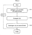
- the Figure 2 shows the method according to the invention in an exemplary form.
- the Figure 3 shows a first embodiment of the step for generating the second total increment, which comprises either an extrapolation or an interpolation of the currently queried total increment.
- the Figure 4 shows a second embodiment of the step for generating the second total increment, in which there is a delay of a polling cycle between the polling of a first total increment and the transmission of the second total increment generated therefrom.
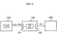
- the Figure 5 shows the device according to the invention and the first unit and the second unit in an exemplary form.
- the Figure 6 shows a first embodiment of the device according to the invention, which is suitable for carrying out the first embodiment of the method according to the invention.
- the Figure 7 shows a second embodiment of the device according to the invention, which is suitable for carrying out the second embodiment of the method according to the invention.
- FIGs 1A and 1B serve to illustrate the problem on which the present invention is based.
- Figure 1A the time course of the data path clocks with the first frequency f a and the accumulator level belonging to each data path clock, that is, the number of partial increments v i accumulated in the accumulator, are shown
- Figure 1B the time course of the interrogation clocks with the second frequency f s and the total increment v 0 interrogated or read out in a respective interrogation clock are shown.
- the number of partial increments v i contained in a total increment v 0 varies between 4 and 5. This pattern repeats itself periodically; in the case shown, the period of this pattern is four query cycles.
- the sequence of the values 4 and 5 for the number of partial increments v i contained in a total increment v 0 is set such that the number of switchovers between the two values becomes a maximum.
- the integral error criterion is completely fulfilled, but the differential error criterion is only insufficiently fulfilled, which is interpreted as additional noise in the data in the querying unit. Therefore, the differential error criterion should be improved with the aid of the method according to the invention, while the integral error criterion continues to be met.
- increment is used as a synonym for a difference in data content between a final value and an initial value.
- total increment stands for the difference in data content, the initial value of the data content being determined at the start of a time interval and the end value of the data content being determined at the end of the time interval.
- the corresponding time interval is referred to as the associated time increment.
- a data content can be a measured variable, for example.
- the Figure 2 shows the method according to the invention in an exemplary form as a block diagram.
- a first total increment v 0 (k) and a first value W (k) are queried from a first unit in a first step S11.
- data also referred to as partial increments of a variable, are accumulated with a first frequency f a , which is also called the data path frequency.
- the first unit can be a sensor, which detects or generates measured values with the first frequency f a and continuously accumulates them in an accumulator.
- An integer number of accumulated partial increments forms the first total increment v 0 (k), the first total increment v 0 (k) corresponding to the data content of the data block present in the first unit at the current query time k, in other words the data content of the accumulated partial increments.
- the accumulation of the data enables the data or measured values to be smoothed over an accumulation interval.
- the first unit generates the first value W (k), which represents a time increment t 0 (k) belonging to the first total increment v 0 (k).
- the first value W (k) can also directly be the time increment t 0 (k) belonging to the first total increment v 0 (k).
- the time increment t 0 (k) corresponds to the accumulation interval, the accumulation interval being the time between the time the last partial increment was generated, which was included in the previous step for querying the first total increment, and the time the last increment was generated in the current step for querying the first total increment is queried partial increments.
- the accumulation interval is therefore always an integral multiple of the data path cycle t a .
- the accumulator content is set to 0 in the first unit.
- the first value W (k) for determining the first value W (k + 1) is also defined in the next query step. For example, the count of the accumulator can be set to 0.
- a second total increment v (k) is generated from the first total increment v 0 (k) using the first value W (k), the second total increment being adapted to the data content of a nominal time increment t s Data blocks.
- the nominal time increment t s corresponds to an integration interval, the integration interval being the time between the time of execution of the previous step for querying the first total increment and the time of execution of the current step for querying the first total increment.
- the second frequency f s and thus the nominal time increment t s are generally specified and assumed to be constant. However, it is also possible to determine the specific value of t s and to include this as the current value of t s in the calculation of the second total increment.
- the generated second total increment v (k) is transmitted to the second unit.
- the second unit can be, for example, an evaluation unit or a further processing unit which evaluates or further processes the data generated or recorded in the first unit and thereby queries the data from the first unit at the second frequency f s .
- the steps for querying the first total increment v 0 (k) and the first value W (k), for generating the second total increment v (k) and for transmitting the second total increment v (k) can be carried out repeatedly at the second frequency f s where the index k increases by 1 each time.
- the method according to the invention leads to an improvement in the differential error criterion, the integral error criterion nevertheless still being met.
- the method according to the invention also has the advantages mentioned for the case that the normally rigid frequency ratio f a / f s varies from the first frequency f a to the second frequency f s for a limited time. This can be caused, for example, by jitter, that is to say fluctuations, in the first frequency f a or in the second frequency f s .
- the step for generating a second total increment according to a first embodiment of the method is shown as a flow diagram.
- the first total increment v 0 (k) and the first value W (k) are queried from the first unit in step S21 and, if the first value W ( k) the not belonging to the first total increment increment of time t 0 (k) directly corresponds to that for the first total increment v 0 (k) belonging increment of time is t 0 (k) W (k).
- step S22 it is decided in step S22 whether or not the index k is equal to 0.
- the first summand represents a possibly not yet processed remaining part from the previous integration interval
- the second summand the largest or the complete part from the current integration interval as well as possibly an extrapolated loan to the still unknown next integration interval and the last summand or the subtrahend a correction increment, which takes into account an extrapolated bond to the current integration interval that may have been used in the previous step to generate a second total increment.
- the second total increment thus corresponds to the sum of a residual portion that may have not yet been processed in the previous step to generate a second total increment, at least part of the first total increment queried in the current step for querying a first total increment, possibly a portion of the current total increment extrapolated in the next step , and optionally a correction increment that corresponds to the negative of the extrapolated portion used in the previous step to generate a second total increment.
- the first total increment v 0 (k) is extrapolated to the next first total increment to be queried carried out. This extrapolation is based on the assumption that the next first total increment to be queried will have the same value as the first total increment currently queried.
- the extrapolated portion of the second total increment corresponds to the correction increment of the next step for generating a second total increment. Since the total time increment t 0 (k) belonging to the current first total increment contributes to the generation of the second total increment v (k), there is no unprocessed remaining portion of the currently queried first total increment for the next step to generate a second total increment.
- step S25 the remaining portion t 1r (k) to be used in the next step to generate a second total increment and the correction increment v r (k) to be used in the next step to generate a second total increment differ for the two cases shown. Therefore, after or before the calculation of the second total increment v (k) in step S25, a distinction is made between cases with regard to the length of the nominal time increment t s, as described above. Depending on this, the state transitions in step S26 or S27, i.e.
- step S29 the index k is now increased by 1 in step S29 and steps S21 to S29 are repeated, the overall process being carried out with the second frequency f s , that is, once per query cycle.
- the step for generating a second total increment according to a second embodiment of the method is shown as a flow diagram.
- the first total increment v 0 (k) and the first value W (k) are queried from the first unit in step S31 and, if the first value W ( k) the not belonging to the first total increment increment of time t 0 (k) directly corresponds to that for the first total increment v 0 (k) belonging increment of time is t 0 (k) W (k).
- step S32 it is decided in step S32 whether or not the index k is 0.
- next step S34 a case distinction is made with regard to the length of the nominal time increment t s compared to the sum of the remaining portion t 2r (k) of the time increment belonging to the previous first total increment and that in the previous step that has not yet been processed in the previous steps for generating a second total increment for generating a second total increment that has not yet been processed residual portion t 1r (k) of the time increment belonging to the previous first total increment.
- the second total increment is thus made up of any remaining portion of the previous first total increment that has not yet been processed, i.e. of the previous integration interval, of the complete remaining portion of the previous first total increment that has not yet been processed, i.e. of the previous integration interval, and a portion of the current first total increments from the current integration interval. Since the total remaining portion of the previous first total increment contributes to the second total increment, no remaining portion of the previous first total increment remains, which would have to be taken into account in the next step for generating a second total increment. A portion of the current first total increment already contributes to the second total increment, so that in the next step for generating a second total increment only a remaining portion of this first total increment has to be taken into account.
- the second total increment is thus made up of any remaining portion of the previous first total increment that has not yet been processed, i.e. of the previous integration interval, as well as of the majority of the previous first total increment, i.e. of the previous integration interval. Since only a part of the previous first total increment contributes to the second total increment, a remainder of the previous first total increment remains, which is to be taken into account in the next step for generating a second total increment. No part of the current first total increment contributes to the second total increment, so that in the next step to generate a second total increment, the complete portion of the current first total increment must be taken into account.
- the second total increment of the sum of, if applicable, a remaining portion of the previous first total increment queried in the previous step for querying a first total increment, which has not yet been processed in the previous step to generate a second total increment, from at least a part of the previous step for querying a first total increment queried previous total increment as well as from optionally a part of the first total increment queried in the current step for querying a first total increment corresponds.
- the index k is now increased by 1 in step S38 and steps S31 to S38 are repeated, the entire process being carried out at the second frequency f s , that is, once per query cycle.
- FIG. 10 shows an apparatus 100 suitable for the process shown in FIG Figure 2 carry out the method described, and a first unit 200 and a second unit 300 in a schematic form.
- the first unit 200 comprises an accumulator 210, the data or partial increments that were generated or detected with a first frequency f a , and a first total increment v 0 (k) and a first value W (k), which is the first total increment associated time increment t 0 (k), that is, the accumulation interval, represents.
- the first unit 200 can, for example be a sensor that generates the data or partial increments with the first frequency f a , the data path clock, and in this case includes further units, for example measuring units and / or processing units. Examples of such a sensor include rotation rate or acceleration sensors. With rotation rate sensors, the partial increments represent partial angle increments, while with acceleration sensors the partial increments are partial speed increments.
- the first unit 200 can also request the data or partial increments from a further unit with the first frequency f a and accumulate them in the accumulator 210.
- the device 100 comprises an input 110 which is suitable for interrogating or receiving the first total increment v 0 (k) and the first value W (k) from the first unit 200 at a second frequency f s , a filter 120 and 160, respectively which is suitable for generating a second total increment v (k) from the first total increment v 0 (k) using the first value W (k), and an output 150 which is suitable for the second total increment v (k) to transmit the second unit 300 at the second frequency f s .
- the second unit 300 can be an evaluation and display unit or any type of further processing unit that queries or receives the second total increment transmitted by the device 100 with the second frequency f s and evaluates, displays and / or processes it accordingly.
- the device 100 enables the data generated with the first frequency f a to be synchronized to the second frequency f s . In this way, the data generated with the first frequency f a can be represented exactly in a polling cycle of the second frequency f s .
- the device 100 enables compliance with the integral error criterion and the improvement of the differential error criterion for mutually independent first and second frequencies f a and f s .
- the device 100 is in Figure 5 shown as an independent unit which is arranged between the first unit 200 and the second unit 300. However, it is also possible that the device 100 is integrated in the first unit 200 or in the second unit 300, whereby the input 110 or the output 150 can be omitted accordingly.
- FIG. 11 shows a first embodiment of the device 100 according to the invention which is suitable for that described with reference to FIG Figure 3 perform described first embodiment of the method according to the invention.
- this embodiment has a filter 120, a memory 145 and a clock generator 146.
- the clock generator 146 can receive a start or an end signal from outside the device 100 and then controls the query of the first total increment v 0 (k) and the first value W (k) from the first unit 200 with the second frequency f s as well as the definition of the index k.
- the start and end signal can be provided by the first unit 200, the second unit 300 or by another device or a user.
- the initial values for the variables required in the filter 120 to calculate the second total increment v (k) are stored in the memory 145 and are made available to the filter 120 when the start signal is received.
- the second frequency f s can be stored in the memory 145.
- the second frequency f s or the nominal time increment t s resulting therefrom can, however, also be provided directly by the second unit 300 or can be determined from a signal sent by the second unit 300.
- the initial values and the nominal time increment are fed from the memory 145 and / or externally to the filter 120.
- the filter has a counter 141 which provides the current value of the index k.
- the index k in the counter 141 is set to zero and is increased by 1 for each further clock pulse given by the clock generator 146. If the value of the index k is equal to zero, the counter 141 sets the initial values, that is to say t 1r (0), t 0 (0), t 1 (0), v 1 (0) and v r (0), the corresponding components of the filter, which are described in more detail below, available.
- the functionalities of different components of the device 100 for example the memory 145, the clock generator 146 and / or the counter 141, to be implemented jointly in one or more components.
- the clock for querying the first total increment and the first value as well as for increasing the index k is supplied from outside, that is, from outside the device 100, so that the device 100 does not have to contain a clock.
- the filter 120 comprises a calculation unit 142 which is suitable for calculating the time increment t 0 (k) belonging to the first total increment v 0 (k) from the queried first value W (k). If the first value W (k) already corresponds to the time increment t 0 (k), the calculation unit 142 can also be omitted.
- the filter 120 further comprises adders 121 to 123, inverters 124 to 127, a two-point element 128, switching elements 129 and 130, delay units 131 to 134, multipliers 135 to 137 and dividers 138 to 140.
- the two-point element 128 provides a signal S at the output and enables the case to be differentiated with regard to the length of the nominal time increments t s compared to the sum of t 1r (k) and t 0 (k).
- the signal S assumes the value S 1
- the signal S assumes the value S 2
- the switching elements 129 and 130 each assume the switch positions belonging to the signal S, so that the output of the switching elements assumes a value belonging to the corresponding case.
- the delay units 131 to 134 represent buffers which forward an input value to the output with a time delay of one cycle of the integration interval, that is to say with a time delay of t s . This means that the input value of a delay unit is available at the output for further processing in the next integration interval.
- the exact connection of the individual components of the filter 120 can be Figure 6 can be removed.
- the filter 120 thus enables the calculation of the second total increment v (k) and the state transitions t 1 (k + 1), v 1 (k + 1), v r (k + 1) and t 1r (k + 1) according to FIG Formulas (6), (7) and (8) or (9) and (10) as well as (11) and (12).
- FIG. 11 shows a first embodiment of the device 100 according to the invention which is suitable for that described with reference to FIG Figure 4 execute described second embodiment of the method according to the invention.
- this embodiment has a filter 160, a memory 145 and a clock generator 146.
- the memory 145 and the clock generator 146 the statements made with reference to FIG. 6 apply.
- the filter has a counter 186 which provides the current value of the index k.
- the index k im Counter 186 Upon receipt of a start signal from the clock 146, the index k im Counter 186 is set to zero and increased by 1 for each further cycle specified by the clock generator 146. If the value of the index k is equal to zero, the counter 186 sets the initial values, that is to say t 2r (0), t 1r (0), t 0 (0), t 2 (0), t 1 (0), v 1 (0) and v 2 (0), the corresponding components of the filter, which will be described in more detail below.
- the filter 160 may include a calculation unit 187 which is suitable for calculating the time increment t 0 (k) belonging to the first total increment v 0 (k) from the queried first value W (k). If the first value W (k) already corresponds to the time increment t 0 (k), the calculation unit 187 can also be omitted.
- the filter 160 comprises for calculating the second total increment v (k) and the state transitions t 1 (k + 1), t 2 (k + 1), vi (k + 1), v 2 (k + 1), t 1r (k + 1) and t 2r (k + 1) adders 161 to 164, inverters 165 to 168, a two-point element 169, switching elements 170 to 173, delay units 174 to 179, multipliers 180 to 182 and dividers 183 to 185 provides a signal S at the output and enables the case to be differentiated with regard to the length of the nominal time increment t s compared to the sum of t 1r (k) and t 2r (k).
- the signal S assumes the value S 1
- the signal S assumes the value S 2
- the switching elements 170 to 173 each assume the switch positions belonging to the signal S, so that the output of the switching elements assumes a value belonging to the corresponding case.
- the delay units 174 to 179 represent buffers which forward an input value to the output with a time delay of one cycle of the integration interval, that is to say with a time delay of t s . This means that the input value of a delay unit is available at the output for further processing in the next integration interval.
- the filter 160 thus enables the calculation of the second total increment v (k) and the state transitions t 1 (k + 1), t 2 (k + 1), v 1 (k + 1), v 2 (k + 1), t 1r (k + 1) and t 2r (k + 1) according to formulas (20) and (23), (21) and (22) respectively (24) and (25) as well as (26) to (29).
Landscapes
- Engineering & Computer Science (AREA)
- Signal Processing (AREA)
- Computer Networks & Wireless Communication (AREA)
- Theoretical Computer Science (AREA)
- Power Engineering (AREA)
- General Physics & Mathematics (AREA)
- Physics & Mathematics (AREA)
- General Engineering & Computer Science (AREA)
- Radar, Positioning & Navigation (AREA)
- Remote Sensing (AREA)
- Synchronisation In Digital Transmission Systems (AREA)
- Mobile Radio Communication Systems (AREA)
- Data Exchanges In Wide-Area Networks (AREA)
- Debugging And Monitoring (AREA)
- Complex Calculations (AREA)
Description
- Bei der Übertragung von Daten zwischen zwei Geräten oder Einheiten, die mit unterschiedlichen Taktfrequenzen arbeiten, ist neben der Sicherstellung der Übertragung aller Daten auch eine Synchronisation der beiden Takte wichtig.
- Die
EP 1 343 261 A1 offenbart ein System zum Extrahieren und Desynchronisieren eines aus einem Multiplexsignal stammenden Signals mit dessen ursprünglichen Datenrate. Dazu werden Signalbits aus dem Multiplexsignal in einem Pufferspeicher zwischengespeichert und mit einer Auslesefrequenz wieder ausgelesen. Die Auslesefrequenz wird basierend auf einem Vergleich der Lese- und Schreibraten des Pufferspeichers in Synchronisation mit der Frame-Rate eingestellt. - Bei einer Übertragung von Daten können beispielsweise in einer ersten Einheit Daten mit einer ersten Taktfrequenz erzeugt werden, die dann von einer zweiten Einheit mit einer zweiten Taktfrequenz, die von der ersten Taktfrequenz verschieden ist, ausgelesen oder abgefragt werden. So werden zum Beispiel in Sensoren Teilinkremente mit einem Datenpfadtakt erzeugt und zunächst akkumuliert. Eine Ausleseeinheit liest den momentanen Stand des Akkumulators mit einem Abfragetakt, so dass im jeweiligen Abfragetakt ein in einem Akkumulationsintervall erzeugtes Gesamtinkrement vom Sensor an die Ausleseeinheit übertragen wird.
- Das Gesamtinkrement wird durch Akkumulation über eine ganzzahlige Anzahl von Datenpfadtakten gebildet. Wenn der Abfragetakt kein ganzzahliges Vielfaches des Datenpfadtaktes ist, wird diese ganzzahlige Anzahl von Datenpfadtakten aber nicht konstant sein. Die Anzahl der Datenpfadtakte wird vielmehr so zwischen zwei ganzzahligen Werten N und N+1 wechseln, dass das sich einstellende Mittel zwischen den N und N+1 Werten dem Verhältnis von Frequenz des Datenpfadtaktes zu Frequenz des Abfragetaktes entspricht. Und selbst wenn der Abfragetakt ein ganzzahliges Vielfaches des Datenpfadtaktes ist, können schon kleinste Abweichungen in den Frequenzen des Datenpfadtaktes oder des Abfragetaktes zu Schwebungseffekten in der Anzahl der Datenpfadtakte führen.
- Damit kann zwar das sogenannte integrale Fehlerkriterium, das angibt, wie gut die Teilinkremente in den Gesamtinkrementen erfasst werden, erfüllt werden, so dass nach einer gewissen Anzahl von Abfragetakten alle mit dem Datenpfadtakt erzeugte Teilinkremente übertragen worden sind. Jedoch wird der Wechsel in der Anzahl der in einem ausgelesenen Gesamtinkrement enthaltenen Teilinkremente in der Ausleseeinheit als zusätzliches Rauschen interpretiert. Das ausgelesene Gesamtinkrement entspricht nicht vollständig der Integration der Daten über den Abfragetakt, wodurch das sogenannte differentielle Fehlerkriterium, das diese Eigenschaft beschreibt, nur unzureichend erfüllt ist.
- Jedoch wird der Wechsel in der Anzahl der in einem ausgelesenen Gesamtinkrement enthaltenen Teilinkremente in der Ausleseeinheit als zusätzliches Rauschen interpretiert. Das ausgelesene Gesamtinkrement entspricht nicht vollständig der Integration der Daten über den Abfragetakt, wodurch das sogenannte differentielle Fehlerkriterium, das diese Eigenschaft beschreibt, nur unzureichend erfüllt ist.
- Es ist daher Aufgabe der vorliegenden Erfindung, ein Verfahren sowie eine Vorrichtung zur Übertragung von Daten an einem asynchronen Übergang zwischen zwei Domänen mit unterschiedlichen Taktfrequenzen zur Verfügung zu stellen, die sowohl das integrale Fehlerkriterium erfüllen als auch das differentielle Fehlerkriterium verbessern.
- Diese Aufgabe wird gelöst durch ein Verfahren und eine Vorrichtung gemäß der unabhängigen Ansprüche. Bevorzugte Ausführungsformen finden sich in den Unteransprüchen.
- Ausführungsformen des erfindungsgemäßen Verfahrens und der erfindungsgemäßen Vorrichtung werden im Folgenden anhand der Figuren näher erläutert, wobei gleichartige Elemente mit gleichen Bezugszeichen gekennzeichnet sind.
- Die
Figur 1A zeigt den zeitlichen Verlauf der Datenpfadtakte sowie die im Akkumulator akkumulierten Teilinkremente. - Die
Figur 1B zeigt den zeitlichen Verlauf der Abfragetakte sowie das im jeweiligen Abfragetakt ausgelesene Gesamtinkrement. - Die
Figur 2 zeigt das erfindungsgemäße Verfahren in einer exemplarischen Form. - Die
Figur 3 zeigt eine erste Ausführungsform des Schrittes zum Erzeugen des zweiten Gesamtinkrements, die entweder eine Extrapolation oder eine Interpolation des momentan abgefragten Gesamtinkrements umfasst. - Die
Figur 4 zeigt eine zweite Ausführungsform des Schrittes zum Erzeugen des zweiten Gesamtinkrements, bei der eine Verzögerung von einem Abfragetakt zwischen dem Abfragen eines ersten Gesamtinkrements und dem Übertragen des daraus erzeugten zweiten Gesamtinkrements auftritt. - Die
Figur 5 zeigt die erfindungsgemäße Vorrichtung sowie die erste Einheit und die zweite Einheit in einer exemplarischen Form. - Die
Figur 6 zeigt eine erste Ausführungsform der erfindungsgemäßen Vorrichtung, die zur Ausführung der ersten Ausführungsform des erfindungsgemäßen Verfahrens geeignet ist. - Die
Figur 7 zeigt eine zweite Ausführungsform der erfindungsgemäßen Vorrichtung, die zur Ausführung der zweiten Ausführungsform des erfindungsgemäßen Verfahrens geeignet ist. - Die
Figuren 1A und 1B dienen zur Verdeutlichung des der vorliegenden Erfindung zugrundeliegenden Problems. InFigur 1A sind der zeitliche Verlauf der Datenpfadtakte mit der ersten Frequenz fa sowie der zu jedem Datenpfadtakt gehörende Akkumulatorstand, das heißt die Anzahl der im Akkumulator akkumulierten Teilinkremente vi, dargestellt, während inFigur 1B der zeitliche Verlauf der Abfragetakte mit der zweiten Frequenz fs sowie das in einem jeweiligen Abfragetakt abgefragte oder ausgelesene Gesamtinkrement v0 dargestellt sind. Beispielhaft wurden die erste Frequenz fa mit 3,4 kHz und die zweite Frequenz fs mit 800 Hz ange-nommen. Demnach besteht ein Abfragetakt aus
- Weil nur über eine ganze Zahl von Datenpfadtakten akkumuliert werden kann, wird zur vollständigen Übertragung aller Daten dreimal über vier Datenpfadtakte und einmal über fünf Datenpfadtakte akkumuliert. Das heißt, die Anzahl der in einem Gesamtinkrement v0 enthaltenen Teilinkremente vi variiert zwischen 4 und 5. Dieses Muster wiederholt sich periodisch, im dargestellten Fall beträgt die Periodendauer dieses Musters vier Abfragetakte. Die Aufeinanderfolge der Werte 4 und 5 für die Anzahl der in einem Gesamtinkrement v0 enthaltenen Teilinkremente vi stellt sich dabei so ein, dass die Zahl der Umschaltungen zwischen beiden Werten maximal wird.
- Mögliche Fehlerarten, die bei dieser Art der Datenabfrage und Integration auftreten können, werden in zwei Klassen unterteilt: Zum Ersten in das integrale Fehlerkriterium, das beurteilt, wie gut die Teilinkremente vi in den Gesamtinkrementen v0 erfasst werden, und zum Zweiten in das differentielle Fehlerkriterium, das beurteilt, wie gut ein Gesamtinkrement v0 der Integration über einen Abfragetakt entspricht.
- In dem dargestellten Beispiel wird das integrale Fehlerkriterium vollständig, das differentielle Fehlerkriterium jedoch nur unzureichend erfüllt, was als ein zusätzliches Rauschen der Daten in der abfragenden Einheit interpretiert wird. Daher soll mit Hilfe des erfindungsgemäßen Verfahrens das differentielle Fehlerkriterium verbessert werden, während das integrale Fehlerkriterium weiterhin erfüllt bleibt.
- Für die Erläuterung des erfindungsgemäßen Verfahrens werden folgende Symbole eingeführt:
- ts
- das zur zweiten Frequenz fs gehörende nominale Zeitinkrement;
- t0(k)
- das zum momentan abgefragten ersten Gesamtinkrement gehörende Zeitinkrement;
- t1(k)
- das zum vorherigen ersten Gesamtinkrement gehörende Zeitinkrement;
- t1r(k)
- der im vorherigen Schritt zum Erzeugen eines zweiten Gesamtinkrements noch nicht verarbeitete Restanteil des zum vorherigen ersten Gesamtinkrement gehörenden Zeitinkrements t1(k);
- v0(k)
- das im momentanen Schritt zum Abfragen eines ersten Gesamtinkrements abgefragte erste Gesamtinkrement;
- v1(k)
- das im vorherigen Schritt zum Abfragen eines ersten Gesamtinkrements abgefragte vorherige erste Gesamtinkrement;
- vr(k)
- der im vorherigen Schritt zum Erzeugen eines zweiten Gesamtinkrements verwendete extrapolierte Anteil, der im momentanen Schritt zum Erzeugen eines zweiten Gesamtinkrements als Korrekturinkrement berücksichtigt werden muss;
- v2(k)
- das im vorvorherigen Schritt zum Abfragen eines ersten Gesamtinkrements abgefragte vorvorherige erste Gesamtinkrement;
- t2(k)
- das zum vorvorherigen ersten Gesamtinkrement gehörende Zeitinkrement;
- t2r(k)
- der in den bisherigen Schritten zum Erzeugen eines zweiten Gesamtinkrements noch nicht verarbeitete Restanteil des zum vorvorherigen ersten Gesamtinkrement gehörenden Zeitinkrements t2(k);
- v(k)
- das auf das nominale Zeitinkrement ts angepasste zweite Gesamtinkrement.
- Der Begriff "Inkrement" wird als Synonym für eine Differenz eines Dateninhalts zwischen einem Endwert und einem Anfangswert verwendet. Beispielsweise steht der Begriff "Gesamtinkrement" für die Differenz eines Dateninhalts, wobei der Anfangswert des Dateninhalts am Beginn eines Zeitintervalls und der Endwert des Dateninhalts am Ende des Zeitintervalls bestimmt werden. Das entsprechende Zeitintervall wird als zugehöriges Zeitinkrement bezeichnet. Ein Dateninhalt kann beispielsweise eine Messgröße sein.
- Die
Figur 2 zeigt das erfindungsgemäße Verfahren in einer exemplarischen Form als Blockdiagramm. Nach dem Start des Verfahrens wird in einem ersten Schritt S11 ein erstes Gesamtinkrement v0(k) sowie ein erster Wert W(k) von einer ersten Einheit abgefragt. In der ersten Einheit werden Daten, auch als Teilinkremente einer Größe bezeichnet, mit einer ersten Frequenz fa, die auch Datenpfadfrequenz genannt wird, akkumuliert. Beispielsweise kann die erste Einheit ein Sensor sein, der Messwerte mit der ersten Frequenz fa erfasst oder erzeugt und diese in einem Akkumulator fortlaufend akkumuliert. Eine ganzzahlige Anzahl von akkumulierten Teilinkrementen bildet das erste Gesamtinkrement v0(k), wobei das erste Gesamtinkrement v0(k) dem Dateninhalt des zum momentanen Abfragezeitpunkt k in der ersten Einheit vorliegenden Datenblocks, mit anderen Worten dem Dateninhalt der akkumulierten Teilinkremente, entspricht. Die Akkumulation der Daten ermöglicht eine Glättung der Daten oder Messwerte über ein Akkumulationsintervall. - Darüber hinaus erzeugt die erste Einheit den ersten Wert W(k), der ein zum ersten Gesamtinkrement v0(k) gehörendes Zeitinkrement t0(k) repräsentiert. Dieser erste Wert W(k) kann beispielsweise ein Zählerstand des Akkumulators sein, der die Anzahl der im ersten Gesamtinkrement v0(k) enthaltenen Teilinkremente wiedergibt und aus dem sich durch Multiplikation mit dem Datenpfadtakt ta = 1/fa das zum ersten Gesamtinkrement v0(k) gehörende Zeitinkrement t0(k) berechnen lässt. Jedoch kann der erste Wert W(k) auch direkt das zum ersten Gesamtinkrement v0(k) gehörende Zeitinkrement t0(k) sein. Das Zeitinkrement t0(k) entspricht dem Akkumulationsintervall, wobei das Akkumulationsintervall die Zeitdauer zwischen dem Zeitpunkt der Erzeugung des letzten Teilinkrements, das im vorherigen Schritt zum Abfragen des ersten Gesamtinkrements enthalten war, und dem Zeitpunkt der Erzeugung des letzten im momentanen Schritt zum Abfragen des ersten Gesamtinkrements abgefragten Teilinkrements ist. Damit ist das Akkumulationsintervall immer ein ganzzahliges Vielfaches des Datenpfadtaktes ta.
- Nach dem Abfragen des ersten Gesamtinkrements v0(k) wird der Akkumulatorinhalt in der ersten Einheit auf 0 gesetzt. Auch wird der erste Wert W(k) für die Bestimmung des ersten Wertes W(k+1) im nächsten Abfrageschritt definiert. Beispielsweise kann der Zählerstand des Akkumulators auf 0 gesetzt werden.
- In einem zweiten Schritt S12 des erfindungsgemäßen Verfahrens wird aus dem ersten Gesamtinkrement v0(k) unter Nutzung des ersten Wertes W(k) ein zweites Gesamtinkrement v(k) erzeugt, wobei das zweite Gesamtinkrement dem Dateninhalt eines auf ein nominales Zeitinkrement ts angepassten Datenblocks entspricht. Das nominale Zeitinkrement ts entspricht einem Integrationsintervall, wobei das Integrationsintervall die Zeitdauer zwischen dem Zeitpunkt der Ausführung des vorherigen Schrittes zum Abfragen des ersten Gesamtinkrements und dem Zeitpunkt der Ausführung des momentanen Schrittes zum Abfragen des ersten Gesamtinkrements ist. Damit entspricht das nominale Zeitinkrement ts einem Abfragetakt mit ts = 1/fs, wobei fs eine zweite Frequenz ist, mit der eine zweite Einheit die in der ersten Einheit akkumulierten Daten abfragt. Die zweite Frequenz fs und damit das nominale Zeitinkrement ts werden im Allgemeinen vorgegeben und als konstant angenommen. Jedoch ist es auch möglich, den konkreten Wert von ts zu bestimmen und diesen als momentanen Wert von ts in die Berechnung des zweiten Gesamtinkrements einzubeziehen.
- In einem dritten Schritt S13 wird das erzeugte zweite Gesamtinkrement v(k) an die zweite Einheit übertragen. Die zweite Einheit kann beispielsweise eine Auswerteeinheit oder eine weiterverarbeitende Einheit sein, die die in der ersten Einheit erzeugten oder erfassten Daten auswertet oder weiterverarbeitet und dabei die Daten aus der ersten Einheit mit der zweiten Frequenz fs abfragt.
- Wie in
Figur 2 dargestellt können die Schritte zum Abfragen des ersten Gesamtinkrements v0(k) und des ersten Wertes W(k), zum Erzeugen des zweiten Gesamtinkrements v(k) sowie zum Übertragen des zweiten Gesamtinkrements v(k) wiederholt mit der zweiten Frequenz fs ausgeführt werden, wobei sich der Index k jeweils um 1 erhöht. - Das erfindungsgemäße Verfahren führt bei beliebigem Verhältnis von erster Frequenz fa zu zweiter Frequenz fs (fa/fs > 1) zu einer Verbesserung des differentiellen Fehlerkriteriums, wobei das integrale Fehlerkriterium trotzdem erfüllt bleibt.
- Dies gilt speziell auch für den Fall, dass die erste Frequenz fa gleich einem ganzzahligen Vielfachen der zweiten Frequenz fs ist.
- Das erfindungsgemäße Verfahren weist die erwähnten Vorteile auch auf für den Fall, dass das normalerweise starre Frequenzverhältnis fa/fs von erster Frequenz fa zu zweiter Frequenz fs zeitlich begrenzt variiert. Dies kann beispielsweise durch einen Jitter, das heißt Schwankungen, in der ersten Frequenz fa oder in der zweiten Frequenz fs verursacht werden.
- In
Figur 3 ist der Schritt zum Erzeugen eines zweiten Gesamtinkrements gemäß einer ersten Ausführungsform des Verfahrens als Flussdiagram dargestellt. Nach dem Start des Verfahrens, bei dem der Index k auf Null gesetzt wird, werden zunächst in Schritt S21 das erste Gesamtinkrement v0(k) und der erste Wert W(k) von der ersten Einheit abgefragt und, falls der erste Wert W(k) nicht dem zum ersten Gesamtinkrement gehörenden Zeitinkrement t0(k) direkt entspricht, wird das zum ersten Gesamtinkrement v0(k) gehörende Zeitinkrement t0(k) aus W(k) berechnet. - Danach wird in Schritt S22 entschieden, ob der Index k gleich 0 ist oder nicht. Für den Fall, dass k=0 ist, werden in Schritt S23 folgende Startwerte für das Erzeugen des zweiten Gesamtinkrements v(k) festgelegt:





- Im nächsten Schritt S24 wird das zweite Gesamtinkrement wie folgt berechnet:

- Dabei repräsentiert der erste Summand einen eventuell noch nicht verarbeiteten Restanteil aus dem vorherigen Integrationsintervall, der zweite Summand den größten oder den kompletten Anteil aus dem aktuellen Integrationsintervall sowie eventuell eine extrapolierte Anleihe auf das noch unbekannte nächste Integrationsintervall und der letzte Summand beziehungsweise der Subtrahend ein Korrekturinkrement, das eine eventuell im vorherigen Schritt zum Erzeugen eines zweiten Gesamtinkrements verwendete extrapolierte Anleihe auf das momentane Integrationsintervall berücksichtigt. Damit entspricht das zweite Gesamtinkrement der Summe aus gegebenenfalls einem im vorherigen Schritt zum Erzeugen eines zweiten Gesamtinkrements noch nicht verarbeiteten Restanteil, zumindest einem Teil des im momentanen Schritt zum Abfragen eines ersten Gesamtinkrements abgefragten ersten Gesamtinkrements, gegebenenfalls einem in den nächsten Schritt extrapolierten Anteil des aktuellen Gesamtinkrements, und gegebenenfalls einem Korrekturinkrement, das dem Negativen des im vorherigen Schritt zum Erzeugen eines zweiten Gesamtinkrements verwendeten extrapolierten Anteils entspricht.
- Um dies näher zu erläutern, wird eine Fallunterscheidung bezüglich der Länge des nominalen Zeitinkrements ts gegenüber der Summe aus dem zum im vorherigen Schritt zum Erzeugen eines zweiten Gesamtinkrements noch nicht verarbeiteten Restanteil t1r(k) des zum vorherigen ersten Gesamtinkrement gehörenden Zeitinkrements und dem zum momentan abgefragten ersten Gesamtinkrement gehörenden Zeitinkrement t0(k) vorgenommen.
- Für den Fall, dass t 1 r.(k) +t 0(k) < ts ist, wird eine Extrapolation des ersten Gesamtinkrements v0(k) auf das nächste abzufragende erste Gesamtinkrement durchgeführt. Diese Extrapolation beruht auf der Annahme, dass das nächste abzufragende erste Gesamtinkrement den gleichen Wert haben wird wie das momentan abgefragte erste Gesamtinkrement. Mit Hilfe dieser Extrapolation wird das zum momentan abgefragten ersten Gesamtinkrement gehörende Zeitinkrement t0(k) bis an das Ende des nominalen Zeitinkrements ts verlängert, so dass im Ergebnis t 1r (k) + t 0 '(k) = ts ist, wobei t0'(k) das verlängerte Zeitinkrement t0(k) ist.
- Der extrapolierte Anteil des zweiten Gesamtinkrements entspricht dem Korrekturinkrement des nächsten Schrittes zum Erzeugen eines zweiten Gesamtinkrements. Da das gesamte zum momentanen ersten Gesamtinkrement gehörende Zeitinkrement t0(k) zur Erzeugung des zweiten Gesamtinkrements v(k) beiträgt, fällt für den nächsten Schritt zum Erzeugen eines zweiten Gesamtinkrements kein noch nicht verarbeiteter Restanteil des momentan abgefragten ersten Gesamtinkrements an.
- Für den Fall, dass t 1r (k) + t 0(k) ≥ ts ist, wird eine Interpolation des ersten Gesamtinkrements v0(k) durchgeführt. Mit Hilfe dieser Interpolation wird das zum momentan abgefragten ersten Gesamtinkrement gehörende Zeitinkrement t0(k) bis an das Ende des nominalen Zeitinkrements ts verkürzt, so dass im Ergebnis t 1r (k) + t 0 '(k) = ts ist, wobei t0'(k) das verkürzte Zeitinkrement t0(k) ist.
- Damit fällt für den nächsten Schritt zum Erzeugen eines zweiten Gesamtinkrements ein noch nicht verarbeiteter Restanteil des momentan abgefragten ersten Gesamtinkrements an. Da es keinen extrapolierten Anteil des zweiten Gesamtinkrements gibt, muss im nächsten Schritt zum Erzeugen eines zweiten Gesamtinkrements kein Korrekturinkrement subtrahiert werden.
- Wie beschrieben unterscheiden sich also der im nächsten Schritt zum Erzeugen eines zweiten Gesamtinkrements zu verwendete Restanteil t1r(k) und das im nächsten Schritt zum Erzeugen eines zweiten Gesamtinkrements zu verwendete Korrekturinkrement vr(k) für die beiden dargestellten Fälle. Daher erfolgt nach oder vor der Berechnung des zweiten Gesamtinkrements v(k) in Schritt S25 eine Fallunterscheidung hinsichtlich der Länge des nominalen Zeitinkrements ts wie oben beschrieben. Davon abhängig werden im Schritt S26 beziehungsweise S27 die Zustandsübergänge, das heißt die im nächsten Schritt zum Erzeugen eines zweiten Gesamtinkrements zu verwendeten Werte von vr(k+1) und t1r(k+1), wie folgt bestimmt:
für den Fall, dass t 1r (k) + t 0(k) < ts:


- Für beide Fälle gleich werden in Schritt S28 die beiden folgenden Zustandsübergänge, das heißt die im nächsten Schritt zum Erzeugen eines zweiten Gesamtinkrements zu verwendeten Werte von t1(k+1) und v1(k+1), wie folgt bestimmt:


- Solange das erfindungsgemäße Verfahren nicht beendet wird, wird nunmehr in Schritt S29 der Index k um 1 erhöht und die Schritte S21 bis S29 werden wiederholt, wobei der Gesamtprozess mit der zweiten Frequenz fs durchgeführt wird, das heißt einmal pro Abfragetakt.
- Simulationen des in
Figur 3 dargestellten Verfahrens unter Verwendung von echten Sensordaten als Teilinkremente ergab, dass nach einem Einschwingvorgang des Verfahrens das zweite Gesamtinkrement das integrale Fehlerkriterium auch im Falle jitterbehafteter Frequenzen fs und fa erfüllt und das differentielle Fehlerkriterium gegenüber dem ersten Gesamtinkrement deutlich verbessert wurde. Abweichungen des zweiten Gesamtinkrements von einem erwarteten Wert, die durch die im Verfahren durchgeführte Extrapolation verursacht wurden, gingen im Sensorrauschen unter. - In
Figur 4 ist der Schritt zum Erzeugen eines zweiten Gesamtinkrements gemäß einer zweiten Ausführungsform des Verfahrens als Flussdiagram dargestellt. Nach dem Start des Verfahrens, bei dem der Index k auf Null gesetzt wird, werden zunächst in Schritt S31 das erste Gesamtinkrement v0(k) und der erste Wert W(k) von der ersten Einheit abgefragt und, falls der erste Wert W(k) nicht dem zum ersten Gesamtinkrement gehörenden Zeitinkrement t0(k) direkt entspricht, wird das zum ersten Gesamtinkrement v0(k) gehörende Zeitinkrement t0(k) aus W(k) berechnet. - Danach wird in Schritt S32 entschieden, ob der Index k gleich 0 ist oder nicht. Für den Fall, dass k=0 ist, werden in Schritt S33 folgende Startwerte für das Erzeugen des zweiten Gesamtinkrements v(k) festgelegt:


- Im nächsten Schritt S34 erfolgt eine Fallunterscheidung hinsichtlich der Länge des nominalen Zeitinkrements ts gegenüber der Summe aus dem in den bisherigen Schritten zum Erzeugen eines zweiten Gesamtinkrements noch nicht verarbeiteten Restanteil t2r(k) des zum vorvorherigen ersten Gesamtinkrement gehörenden Zeitinkrements und dem im vorherigen Schritt zum Erzeugen eines zweiten Gesamtinkrements noch nicht verarbeiteten Restanteil t1r(k) des zum vorherigen ersten Gesamtinkrement gehörenden Zeitinkrements.
- Für den Fall, dass t 2r (k) + t 1r (k) < ts ist, wird das zweite Gesamtinkrement in Schritt S35 wie folgt berechnet:

- Damit setzt sich das zweite Gesamtinkrement aus eventuell dem bisher noch nicht verarbeiteten Restanteil des vorvorherigen ersten Gesamtinkrements, das heißt aus dem vorvorherigen Integrationsintervall, aus dem kompletten noch nicht verarbeiteten Restanteil des vorherigen ersten Gesamtinkrements, das heißt aus dem vorherigen Integrationsintervall, sowie aus einem Anteil des momentanen ersten Gesamtinkrements aus dem aktuellen Integrationsintervall zusammen. Da der gesamte Restanteil des vorherigen ersten Gesamtinkrements zum zweiten Gesamtinkrement beiträgt, verbleibt kein Restanteil des vorherigen ersten Gesamtinkrements, der im nächsten Schritt zur Erzeugung eines zweiten Gesamtinkrements zu berücksichtigen wäre. Vom momentanen ersten Gesamtinkrement trägt bereits ein Anteil zum zweiten Gesamtinkrement bei, so dass im nächsten Schritt zur Erzeugung eines zweiten Gesamtinkrements nur noch ein Restanteil dieses ersten Gesamtinkrements zu berücksichtigen ist. Damit ergeben sich folgende Zustandsübergänge für den nächsten Schritt zum Erzeugen eines zweiten Gesamtinkrements, die ebenfalls in Schritt S35 berechnet werden:


- Für den Fall, dass t 2r (k)+t 1r (k)≥ts ist, wird das zweite Gesamtinkrement in Schritt S36 wie folgt berechnet:

- Damit setzt sich das zweite Gesamtinkrement aus eventuell dem bisher noch nicht verarbeiteten Restanteil des vorvorherigen ersten Gesamtinkrements, das heißt aus dem vorvorherigen Integrationsintervall, sowie aus dem größten Teil des vorherigen ersten Gesamtinkrements, das heißt aus dem vorherigen Integrationsintervall, zusammen. Da nur ein Teil des vorherigen ersten Gesamtinkrements zum zweiten Gesamtinkrement beiträgt, verbleibt ein Restanteil des vorherigen ersten Gesamtinkrements, der im nächsten Schritt zur Erzeugung eines zweiten Gesamtinkrements zu berücksichtigen ist. Vom momentanen ersten Gesamtinkrement trägt noch kein Teil zum zweiten Gesamtinkrement bei, so dass im nächsten Schritt zur Erzeugung eines zweiten Gesamtinkrements der komplette Anteil des momentanen ersten Gesamtinkrements zu berücksichtigen ist. Damit ergeben sich folgende Zustandsübergänge für den nächsten Schritt zum Erzeugen eines zweiten Gesamtinkrements, die ebenfalls in Schritt S36 berechnet werden:


- Allgemein kann gesagt werden, dass das zweite Gesamtinkrement der Summe aus gegebenenfalls einem im vorvorherigen Schritt zum Erzeugen eines zweiten Gesamtinkrements noch nicht verarbeiteten Restanteil des im vorvorherigen Schritt zum Abfragen eines ersten Gesamtinkrements abgefragten vorvorherigen ersten Gesamtinkrements, aus zumindest einem Teil des im vorherigen Schritt zum Abfragen eines ersten Gesamtinkrements abgefragten vorherigen Gesamtinkrements sowie aus gegebenenfalls einem Teil des im momentanen Schritt zum Abfragen eines ersten Gesamtinkrements abgefragten ersten Gesamtinkrements entspricht. Damit tritt eine Verzögerung von einem Abfragetakt zwischen dem Schritt des Abfragens eines ersten Gesamtinkrements von der ersten Einheit und dem Schritt des Übertragens eines zu diesem abgefragten ersten Gesamtinkrement korrespondierenden zweiten Gesamtinkrements auf.
- Für beide Fälle gleich werden in Schritt S37 die folgenden Zustandsübergänge, das heißt die im nächsten Schritt zum Erzeugen eines zweiten Gesamtinkrements zu verwendeten Werte, bestimmt:



- Solange das erfindungsgemäße Verfahren nicht beendet wird, wird nunmehr in Schritt S38 der Index k um 1 erhöht und die Schritte S31 bis S38 werden wiederholt, wobei der Gesamtprozess mit der zweiten Frequenz fs durchgeführt wird, das heißt einmal pro Abfragetakt.
- Simulationen des in
Figur 4 dargestellten Verfahrens unter Verwendung von echten Sensordaten als Teilinkremente ergab, dass nach einem Einschwingvorgang des Verfahrens das zweite Gesamtinkrement sowohl das integrale Fehlerkriterium als auch das differentielle Fehlerkriterium auch im Falle jitterbehafteter Frequenzen fs und fa erfüllt. - Damit ist das in
Figur 4 dargestellte Verfahren gegenüber dem inFigur 3 dargestellten Verfahren robuster gegenüber einem Jitter in der ersten Frequenz fa oder der zweiten Frequenz fs. Jedoch ergibt sich eine Verzögerung von einem Abfragetakt 1/fs zwischen dem ersten Gesamtinkrement und dem zu diesem gehörigen zweiten Gesamtinkrement, das heißt desjenigen zweiten Gesamtinkrements, in dem das erste Gesamtinkrement zumindest zum Teil enthalten ist. Damit ist das inFigur 4 dargestellte Verfahren besonders für Verfahren zur Übertragung von Daten geeignet, bei denen eine solche Verzögerung entweder keine Rolle spielt oder bei denen eine solche Verzögerung bei der weiteren Verarbeitung der Daten berücksichtigt werden kann. - Die
Figur 5 zeigt eine Vorrichtung 100, die geeignet ist, das inFigur 2 beschriebene Verfahren auszuführen, sowie eine erste Einheit 200 und eine zweite Einheit 300 in einer schematischen Form. - Die erste Einheit 200 umfasst einen Akkumulator 210, der Daten oder Teilinkremente, die mit einer ersten Frequenz fa erzeugt oder erfasst wurden, akkumuliert und ein erstes Gesamtinkrement v0(k) sowie einen ersten Wert W(k), der das zum ersten Gesamtinkrement gehörende Zeitinkrement t0(k), das heißt das Akkumulationsintervall, repräsentiert, bereitstellt. Die erste Einheit 200 kann beispielsweise ein Sensor sein, der die Daten oder Teilinkremente mit der ersten Frequenz fa, dem Datenpfadtakt, erzeugt und in diesem Falle weitere Einheiten, beispielsweise Messeinheiten und/oder Verarbeitungseinheiten, umfasst. Beispiele für einen solchen Sensor sind unter anderem Drehraten- oder Beschleunigungssensoren. Bei Drehratensensoren stellen die Teilinkremente Teilwinkelinkremente dar, während bei Beschleunigungssensoren die Teilinkremente Teilgeschwindigkeitsinkremente sind. Alternativ kann die erste Einheit 200 die Daten oder Teilinkremente auch von einer weiteren Einheit mit der ersten Frequenz fa abfragen und im Akkumulator 210 akkumulieren.
- Die erfindungsgemäße Vorrichtung 100 umfasst einen Eingang 110, der geeignet ist, das erste Gesamtinkrement v0(k) und den ersten Wert W(k) von der ersten Einheit 200 mit einer zweiten Frequenz fs abzufragen oder zu empfangen, einen Filter 120 beziehungsweise 160, der geeignet ist, aus dem ersten Gesamtinkrement v0(k) unter Nutzung des ersten Wertes W(k) ein zweites Gesamtinkrement v(k) zu erzeugen, und einen Ausgang 150, der geeignet ist, das zweite Gesamtinkrement v(k) an die zweite Einheit 300 mit der zweiten Frequenz fs zu übertragen.
- Die zweite Einheit 300 kann eine Auswerte- und Anzeigeeinheit oder eine beliebige Art von weiterverarbeitender Einheit sein, die das von der Vorrichtung 100 übertragene zweite Gesamtinkrement mit der zweiten Frequenz fs abfragt oder empfängt und entsprechend auswertet, anzeigt und/oder weiterverarbeitet.
- Die Vorrichtung 100 ermöglicht das Synchronisieren der mit der ersten Frequenz fa erzeugten Daten auf die zweite Frequenz fs. Damit können die mit der ersten Frequenz fa erzeugten Daten exakt in einem Abfragetakt der zweiten Frequenz fs repräsentiert werden. Insbesondere ermöglicht die Vorrichtung 100 die Einhaltung des integralen Fehlerkriteriums und die Verbesserung des differentiellen Fehlerkriteriums für voneinander unabhängige erste und zweite Frequenzen fa und fs.
- Die Vorrichtung 100 ist in
Figur 5 als selbständige Einheit, die zwischen der ersten Einheit 200 und der zweiten Einheit 300 angeordnet ist, dargestellt. Jedoch ist es auch möglich, dass die Vorrichtung 100 in der ersten Einheit 200 oder in der zweiten Einheit 300 integriert ist, wodurch entsprechend der Eingang 110 oder der Ausgang 150 entfallen können. - Die
Figur 6 zeigt eine erste Ausführungsform der erfindungsgemäßen Vorrichtung 100, die geeignet ist, die mit Bezug auf dieFigur 3 beschriebene erste Ausführungsform des erfindungsgemäßen Verfahrens auszuführen. - Neben dem bereits erwähnten Eingang 110 und dem Ausgang 150 weist diese Ausführungsform einen Filter 120, einen Speicher 145 und einen Taktgeber 146 auf. Der Taktgeber 146 kann von außerhalb der Vorrichtung 100 ein Start- oder ein End-Signal erhalten und steuert dann mit der zweiten Frequenz fs die Abfrage des ersten Gesamtinkrements v0(k) und des ersten Wertes W(k) von der ersten Einheit 200 sowie die Festlegung des Indexes k. Das Start- und Ende-Signal kann von der ersten Einheit 200, der zweiten Einheit 300 oder von einem anderen Gerät oder einem Nutzer bereitgestellt werden.
- Im Speicher 145 sind die Anfangswerte für die im Filter 120 zur Berechnung des zweiten Gesamtinkrements v(k) notwendigen Größen gespeichert und werden bei Empfang des Start-Signals dem Filter 120 zur Verfügung gestellt. Darüber hinaus kann die zweite Frequenz fs im Speicher 145 gespeichert sein. Die zweite Frequenz fs beziehungsweise das daraus resultierende nominale Zeitinkrement ts kann aber auch von der zweiten Einheit 300 direkt bereitgestellt oder aus einem von der zweiten Einheit 300 gesendeten Signal bestimmt werden. Die Anfangswerte sowie das nominale Zeitinkrement werden vom Speicher 145 und/oder von außen dem Filter 120 zugeführt.
- Der Filter weist einen Zähler 141 auf, der den aktuellen Wert des Indexes k bereitstellt. Bei Erhalt eines Start-Signals vom Taktgeber 146 wird der Index k im Zähler 141 auf Null gesetzt und bei jedem weiteren vom Taktgeber 146 vorgegebenen Takt um 1 erhöht. Ist der Wert des Indexes k gleich Null, so stellt der Zähler 141 die Anfangswerte, das heißt t1r(0), t0(0), t1(0), v1(0) und vr(0), den entsprechenden Komponenten des Filters, die nachstehend genauer beschrieben werden, zur Verfügung.
- Es ist möglich, dass die Funktionalitäten verschiedener Komponenten der Vorrichtung 100, beispielsweise des Speichers 145, des Taktgebers 146 und/oder des Zählers 141, in einer oder mehreren Komponenten gemeinsam realisiert werden. Weiterhin ist es auch möglich, dass der Takt zum Abfragen des ersten Gesamtinkrements und des ersten Wertes sowie zum Erhöhen des Indexes k von außen, das heißt von außerhalb der Vorrichtung 100, zugeführt wird, so dass die Vorrichtung 100 keinen Taktgeber enthalten muss.
- Der Filter 120 umfasst eine Berechnungseinheit 142, die geeignet ist, aus dem abgefragten ersten Wert W(k) das zum ersten Gesamtinkrement v0(k) gehörende Zeitinkrement t0(k) zu berechnen. Entspricht der erste Wert W(k) bereits dem Zeitinkrement t0(k), so kann die Berechnungseinheit 142 auch entfallen.
- Zur Berechnung des zweiten Gesamtinkrements v(k) sowie der Zustandsübergänge t1(k+1), v1(k+1), vr(k+1) und t1r(k+1) umfasst der Filter 120 weiterhin Addierer 121 bis 123, Inverter 124 bis 127, ein Zweipunktglied 128, Schaltglieder 129 und 130, Verzögerungseinheiten 131 bis 134, Multiplizierer 135 bis 137 sowie Dividierer 138 bis 140. Das Zweipunktglied 128 stellt ein Signal S am Ausgang bereit und ermöglicht die Fallunterscheidung hinsichtlich der Länge des nominalen Zeitinkrements ts im Vergleich zur Summe aus t1r(k) und t0(k). Für den Fall, dass t 1r (k)+t 0(k) < ts ist, nimmt das Signal S den Wert S1 an, während für den Fall, dass t 1r (k) + t 0(k)≥ts. ist, das Signal S den Wert S2 annimmt. Die Schaltglieder 129 und 130 nehmen jeweils die zum Signal S gehörenden Schalterstellungen an, so dass der Ausgang der Schaltglieder ein zu dem entsprechenden Fall gehörenden Wert annimmt. Die Verzögerungseinheiten 131 bis 134 stellen Zwischenspeicher dar, die einen Eingangswert mit einer Zeitverzögerung von einem Takt des Integrationsintervalls, das heißt mit einer Zeitverzögung von ts, an den Ausgang weiterleiten. Damit steht der Eingangswert einer Verzögerungseinheit im nächsten Integrationsintervall am Ausgang zur weiteren Verarbeitung zur Verfügung.
- Die genaue Verschaltung der einzelnen Komponenten des Filters 120 kann der
Figur 6 entnommen werden. Damit ermöglicht der Filter 120 die Berechnung des zweiten Gesamtinkrements v(k) sowie der Zustandsübergänge t1(k+1), v1(k+1), vr(k+1) und t1r(k+1) gemäß der Formeln (6), (7) und (8) beziehungsweise (9) und (10) sowie (11) und (12). - Die
Figur 7 zeigt eine erste Ausführungsform der erfindungsgemäßen Vorrichtung 100, die geeignet ist, die mit Bezug auf dieFigur 4 beschriebene zweite Ausführungsform des erfindungsgemäßen Verfahrens auszuführen. - Neben dem bereits erwähnten Eingang 110 und dem Ausgang 150 weist diese Ausführungsform einen Filter 160, einen Speicher 145 und einen Taktgeber 146 auf. Bezüglich des Speichers 145 und des Taktgebers 146 gelten die mit Bezug auf Figur 6 gemachten Aussagen.
- Der Filter weist einen Zähler 186 auf, der den aktuellen Wert des Indexes k bereitstellt. Bei Erhalt eines Start-Signals vom Taktgeber 146 wird der Index k im Zähler 186 auf Null gesetzt und bei jedem weiteren vom Taktgeber 146 vorgegebenen Takt um 1 erhöht. Ist der Wert des Indexes k gleich Null, so stellt der Zähler 186 die Anfangswerte, das heißt t2r(0), t1r(0), t0(0), t2(0), t1(0), v1(0) und v2(0), den entsprechenden Komponenten des Filters, die nachstehend genauer beschrieben werden, zur Verfügung.
- Es ist möglich, dass die Funktionalitäten verschiedener Komponenten der Vorrichtung 100, beispielsweise des Speichers 145, des Taktgebers 146 und/oder des Zählers 186, in einer oder mehreren Komponenten gemeinsam realisiert werden oder dass der Taktgeber 146 weggelassen werden kann, wie dies mit Bezug auf
Figur 6 beschrieben ist. - Ähnlich wie mit Bezug auf
Figur 6 beschrieben, kann der Filter 160 eine Berechnungseinheit 187 umfassen, die geeignet ist, aus dem abgefragten ersten Wert W(k) das zum ersten Gesamtinkrement v0(k) gehörende Zeitinkrement t0(k) zu berechnen. Entspricht der erste Wert W(k) bereits dem Zeitinkrement t0(k), so kann die Berechnungseinheit 187 auch entfallen. - Weiterhin umfasst der Filter 160 zur Berechnung des zweiten Gesamtinkrements v(k) sowie der Zustandsübergänge t1(k+1), t2(k+l), vi(k+l), v2(k+1), t1r(k+1) und t2r(k+1) Addierer 161 bis 164, Inverter 165 bis 168, ein Zweipunktglied 169, Schaltglieder 170 bis 173, Verzögerungseinheiten 174 bis 179, Multiplizierer 180 bis 182 sowie Dividierer 183 bis 185. Das Zweipunktglied 169 stellt ein Signal S am Ausgang bereit und ermöglicht die Fallunterscheidung hinsichtlich der Länge des nominalen Zeitinkrements ts im Vergleich zur Summe aus t1r(k) und t2r(k). Für den Fall, dass t 1r (k) + t 2r (k) < ts ist, nimmt das Signal S den Wert S1 an, während für den Fall, dass t 1r (k) + t 2r (k) ≥ ts ist, das Signal S den Wert S2 annimmt. Die Schaltglieder 170 bis 173 nehmen jeweils die zum Signal S gehörenden Schalterstellungen an, so dass der Ausgang der Schaltglieder ein zu dem entsprechenden Fall gehörenden Wert annimmt. Die Verzögerungseinheiten 174 bis 179 stellen Zwischenspeicher dar, die einen Eingangswert mit einer Zeitverzögerung von einem Takt des Integrationsintervalls, das heißt mit einer Zeitverzögung von ts, an den Ausgang weiterleiten. Damit steht der Eingangswert einer Verzögerungseinheit im nächsten Integrationsintervall am Ausgang zur weiteren Verarbeitung zur Verfügung.
- Die genaue Verschaltung der einzelnen Komponenten des Filters 160 kann der
Figur 7 entnommen werden. Damit ermöglicht der Filter 160 die Berechnung des zweiten Gesamtinkrements v(k) sowie der Zustandsübergänge t1(k+1), t2(k+1), v1(k+1), v2(k+1), t1r(k+1) und t2r(k+1) gemäß der Formeln (20) beziehungsweise (23), (21) und (22) beziehungsweise (24) und (25) sowie (26) bis (29).
Claims (15)
- Verfahren zum Übertragen von Daten zwischen einer ersten Einheit, die Daten, die mit einer ersten Frequenz, fa, erzeugt wurden, akkumuliert, und einer zweiten Einheit, die die akkumulierten Daten mit einer zweiten Frequenz, fs, abfragt, die kleiner als die erste Frequenz, fa, ist, umfassend:Abfragen eines ersten Gesamtinkrements, v0(k), und eines ersten Wertes, W(k), der ein zum ersten Gesamtinkrement, v0(k), gehörendes Zeitinkrement, t0(k), repräsentiert, von der ersten Einheit, wobei das erste Gesamtinkrement, vo(k), der Dateninhalt des zum Abfragezeitpunkt, k, in der ersten Einheit vorliegenden akkumulierten Datenblocks ist,Erzeugen eines zweiten Gesamtinkrements, v(k), aus dem ersten Gesamtinkrement, v0(k), unter Nutzung des ersten Wertes, W(k), wobei das zweite Gesamtinkrement, v(k), der Dateninhalt eines auf ein nominales Zeitinkrement, ts, der zweiten Frequenz, fs, angepassten Datenblocks ist, undÜbertragen des zweiten Gesamtinkrements, v(k), an die zweite Einheit.
- Verfahren nach Anspruch 1,
dadurch gekennzeichnet, dass:
die Schritte zum Abfragen eines ersten Gesamtinkrements, v0(k), und eines ersten Wertes, W(k), zum Erzeugen eines zweiten Gesamtinkrements, v(k), und zum Übertragen des zweiten Gesamtinkrements, v(k), wiederholt mit der zweiten Frequenz, fs, ausgeführt werden. - Verfahren nach Anspruch 2,
dadurch gekennzeichnet, dass:
das zweite Gesamtinkrement, v(k), wie folgt berechnet wird: v1(k) das im vorherigen Schritt zum Abfragen eines ersten Gesamtinkrements abgefragte vorherige erste Gesamtinkrement ist,t1(k) das zum vorherigen ersten Gesamtinkrement gehörende Zeitinkrement ist,t1r(k) der im vorherigen Schritt zum Erzeugen eines zweiten Gesamtinkrements noch nicht verarbeitete Restanteil des zum vorherigen ersten Gesamtinkrement gehörenden Zeitinkrements t1(k) ist,v0(k) das im momentanen Schritt zum Abfragen des ersten Gesamtinkrements abgefragte erste Gesamtinkrement ist,ts das zur zweiten Frequenz, fs, gehörende nominale Zeitinkrement ist,t0(k) das zum im momentanen Schritt zum Abfragen des ersten Gesamtinkrements abgefragten ersten Gesamtinkrement gehörende Zeitinkrement ist, undvr(k) der im vorherigen Schritt zum Erzeugen des zweiten Gesamtinkrements verwendete extrapolierte Anteil ist, der im momentanen Schritt zum Erzeugen des zweiten Gesamtinkrements wieder subtrahiert werden muss.
 - Verfahren nach Anspruch 3,
dadurch gekennzeichnet, dass
für k=0 folgende Anfangsbedingungen gewählt werden:


- Verfahren nach Anspruch 3,
dadurch gekennzeichnet, dass
die im nächsten Schritt zum Erzeugen des zweiten Gesamtinkrements, v(k), zu verwendeten Werte von t1(k+l), v1(k+1), t1r(k+1) und vr(k+1) wie folgt berechnet werden:

für den Fall, dass t 1r (k) + t 0(k) <ts:


- Verfahren nach Anspruch 2,
dadurch gekennzeichnet, dass
das zweite Gesamtinkrement, v(k), wie folgt berechnet wird:- für den Fall, dass t 2r (k) + t 1r (k) < ts: - für den Fall, dass t 2r(k) + t 1r (k) ≥ ts:wobei
 v1(k) das im vorherigen Schritt zum Abfragen eines ersten Gesamtinkrements abgefragte vorherige erste Gesamtinkrement ist,v2(k) das im vorvorherigen Schritt zum Abfragen eines ersten Gesamtinkrements abgefragte vorvorherige erste Gesamtinkrement ist,t1(k) das zum vorherigen ersten Gesamtinkrement gehörende Zeitinkrement ist,t1r(k) der im vorherigen Schritt zum Erzeugen eines zweiten Gesamtinkrements noch nicht verarbeitete Restanteil des zum vorherigen ersten Gesamtinkrement gehörenden Zeitinkrements t1(k) ist,t2(k) das zum vorvorherigen ersten Gesamtinkrement gehörende Zeitinkrement ist,t2r(k) der in den bisherigen Schritten zum Erzeugen eines zweiten Gesamtinkrements noch nicht verarbeitete Restanteil des zum vorvorherigen ersten Gesamtinkrement gehörenden Zeitinkrements t2(k) ist,v0(k) das im momentanen Schritt zum Abfragen des ersten Gesamtinkrements abgefragte erste Gesamtinkrement ist,ts das zur zweiten Frequenz, fs, gehörende nominale Zeitinkrement ist, undt0(k) das zum im momentanen Schritt zum Abfragen des ersten Gesamtinkrements abgefragten ersten Gesamtinkrement gehörende Zeitinkrement ist.
 - Verfahren nach Anspruch 6,
dadurch gekennzeichnet, dass
für k=0 folgende Anfangsbedingungen gewählt werden:


- Verfahren nach Anspruch 6,
dadurch gekennzeichnet, dass
die im nächsten Schritt zum Erzeugen des zweiten Gesamtinkrements, v(k), zu verwendeten Werte von t1(k+1), t2(k+1), v1(k+1), v2(k+1), t1r(k+1) und t2r(k+1) wie folgt berechnet werden:


für den Fall, dass t 2r (k)+t 1r (k)<ts:


- Vorrichtung zum Übertragen von Daten zwischen einer ersten Einheit, die Daten, die mit einer ersten Frequenz, fa, erzeugt wurden, akkumuliert, und einer zweiten Einheit, die die akkumulierten Daten mit einer zweiten Frequenz, fs, abfragt, die kleiner als die erste Frequenz, fa, ist, umfassend:einen Eingang, der geeignet ist, ein erstes Gesamtinkrement, v0(k), und einen ersten Wert, W(k), der ein zum ersten Gesamtinkrement, v0(k), gehörendes Zeitinkrement, t0(k), repräsentiert, von der ersten Einheit mit der zweiten Frequenz, fs, abzufragen, wobei das erste Gesamtinkrement, v0(k), der Dateninhalt des zum Abfragezeitpunkt in der ersten Einheit vorliegenden akkumulierten Datenblocks ist,einen Filter, der geeignet ist, aus dem ersten Gesamtinkrement, v0(k), und dem ersten Wert, W(k), ein zweites Gesamtinkrement, v(k), zu erzeugen, wobei das zweite Gesamtinkrement, v(k), der Dateninhalt eines auf ein nominales Zeitinkrement, ts, der zweiten Frequenz, fs, angepassten Datenblocks ist, undeinen Ausgang, der geeignet ist, das zweite Gesamtinkrement, v(k), an die zweite Einheit mit der zweiten Frequenz, fs, zu übertragen.
- Vorrichtung nach Anspruch 9,
dadurch gekennzeichnet dass,
der Filter geeignet ist, das zweite Gesamtinkrement, v(k), wie folgt zu berechnen: v1(k) das im vorherigen Abfragetakt der zweiten Frequenz, fs, abgefragte vorherige erste Gesamtinkrement ist,t1(k) das zum vorherigen ersten Gesamtinkrement gehörende Zeitinkrement ist,t1r(k) der beim vorherigen Erzeugen eines zweiten Gesamtinkrements noch nicht verarbeiteten Restanteil des zum vorherigen ersten Gesamtinkrement gehörenden Zeitinkrements t1(k) ist,v0(k) das im momentanen Abfragetakt der zweiten Frequenz, fs, abgefragte erste Gesamtinkrement ist,ts das zur zweiten Frequenz, fs, gehörende nominale Zeitinkrement ist,t0(k) das zum im momentanen Abfragetakt der zweiten Frequenz, fs, abgefragten ersten Gesamtinkrement gehörende Zeitinkrement ist, undvr(k) der beim vorherigen Erzeugen des zweiten Gesamtinkrements verwendete extrapolierte Anteil ist, der im momentanen Schritt zum Erzeugen des zweiten Gesamtinkrements wieder subtrahiert werden muss.
 - Vorrichtung nach Anspruch 10,
dadurch gekennzeichnet, dass
der Filter einen Startwertgeber umfasst, der geeignet ist, für k=0 folgende Anfangsbedingungen bereitzustellen:


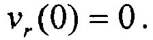
- Vorrichtung nach Anspruch 10,
dadurch gekennzeichnet, dass
der Filter geeignet ist, die beim nächsten Erzeugen eines zweiten Gesamtinkrements, v(k+1), zu verwendeten Werte von t1(k+1), v1(k+1),t1r(k+1) und vr(k+1) wie folgt zu berechnen:

für den Fall, dass t 1r (k) + t0(k) < ts:
 vr (k+1) = 0 undt 1r (k+1)=t 0(k)+t 1r (k)-ts.
 - Vorrichtung nach Anspruch 9,
dadurch gekennzeichnet dass,
der Filter geeignet ist, das zweite Gesamtinkrement, v(k), wie folgt zu berechnen:- für den Fall, dass t 2r (k) + t 1r (k)< ts: - für den Fall, dass t 2r (k)+ t 1r (k) ≥ ts:
 v1(k) das im vorherigen Abfragetakt der zweiten Frequenz, fs, abgefragte vorherige erste Gesamtinkrement ist,v2(k) das im vorvorherigen Abfragetakt der zweiten Frequenz, fs, abgefragte vorvorherige erste Gesamtinkrement ist,t1(k) das zum vorherigen ersten Gesamtinkrement gehörende Zeitinkrement ist,t1r(k) der beim vorherigen Erzeugen eines zweiten Gesamtinkrements noch nicht verarbeitete Restanteil des zum vorherigen ersten Gesamtinkrement gehörenden Zeitinkrements t1(k) ist,t2(k) das zum vorvorherigen ersten Gesamtinkrement gehörende Zeitinkrement ist,t2r(k) der beim bisherigen Erzeugen eines zweiten Gesamtinkrements noch nicht verarbeitete Restanteil des zum vorvorherigen ersten Gesamtinkrement gehörenden Zeitinkrements t2(k) ist,v0(k) das im momentanen Abfragetakt der zweiten Frequenz, fs, abgefragte erste Gesamtinkrement ist,ts das zur zweiten Frequenz, fs, gehörende nominale Zeitinkrement ist, undt0(k) das zum im momentanen Abfragetakt der zweiten Frequenz, fs, abgefragten ersten Gesamtinkrement gehörende Zeitinkrement ist.
 - Vorrichtung nach Anspruch 13,
dadurch gekennzeichnet, dass
der Filter einen Startwertgeber umfasst, der geeignet ist, für k=0 folgende Anfangsbedingungen bereitzustellen:


- Vorrichtung nach Anspruch 13,
dadurch gekennzeichnet, dass
der Filter geeignet ist, die beim nächsten Erzeugen eines zweiten Gesamtinkrements, v(k+1), zu verwendeten Werte von t1(k+1), t2(k+1). v1(k+1), v2(k+1), t1r(k+1) und t2r(k+1) wie folgt zu berechnen:


für den Fall, dass t 2r (k) + t 1r (k) < ts:



Applications Claiming Priority (2)
| Application Number | Priority Date | Filing Date | Title |
|---|---|---|---|
| DE102013020954.4A DE102013020954A1 (de) | 2013-12-12 | 2013-12-12 | Verfahren und Vorrichtung zum Übertragen von Daten an asynchronen Übergängen zwischen Domänen mit unterschiedlichen Taktfrequenzen |
| PCT/EP2014/003229 WO2015086131A1 (de) | 2013-12-12 | 2014-12-03 | Verfahren und vorrichtung zum übertragen von daten an asynchronen übergängen zwischen domänen mit unterschiedlichen taktfrequenzen |
Publications (2)
| Publication Number | Publication Date |
|---|---|
| EP3080944A1 EP3080944A1 (de) | 2016-10-19 |
| EP3080944B1 true EP3080944B1 (de) | 2021-01-20 |
Family
ID=52273069
Family Applications (1)
| Application Number | Title | Priority Date | Filing Date |
|---|---|---|---|
| EP14821062.8A Active EP3080944B1 (de) | 2013-12-12 | 2014-12-03 | Verfahren und vorrichtung zum übertragen von daten an asynchronen übergängen zwischen domänen mit unterschiedlichen taktfrequenzen |
Country Status (13)
| Country | Link |
|---|---|
| US (1) | US10211973B2 (de) |
| EP (1) | EP3080944B1 (de) |
| JP (1) | JP6383790B2 (de) |
| KR (1) | KR101824050B1 (de) |
| CN (1) | CN105794143B (de) |
| AU (1) | AU2014361266B2 (de) |
| BR (1) | BR112016010733B1 (de) |
| CA (1) | CA2928965C (de) |
| DE (1) | DE102013020954A1 (de) |
| IL (1) | IL245620A (de) |
| RU (1) | RU2639956C1 (de) |
| WO (1) | WO2015086131A1 (de) |
| ZA (1) | ZA201602937B (de) |
Families Citing this family (2)
| Publication number | Priority date | Publication date | Assignee | Title |
|---|---|---|---|---|
| DE102013020954A1 (de) * | 2013-12-12 | 2015-06-18 | Northrop Grumman Litef Gmbh | Verfahren und Vorrichtung zum Übertragen von Daten an asynchronen Übergängen zwischen Domänen mit unterschiedlichen Taktfrequenzen |
| DE102019100507B4 (de) | 2019-01-10 | 2025-09-25 | Northrop Grumman Litef Gmbh | Verfahren zum Auslesen von Daten von Inertialsensoren |
Family Cites Families (53)
| Publication number | Priority date | Publication date | Assignee | Title |
|---|---|---|---|---|
| SU1242968A1 (ru) * | 1984-11-23 | 1986-07-07 | Предприятие П/Я Г-4149 | Буферное запоминающее устройство |
| US5206636A (en) * | 1989-10-25 | 1993-04-27 | Motorola, Inc. | Signal search method for selective call receiver |
| FR2655794A1 (fr) * | 1989-12-13 | 1991-06-14 | Cit Alcatel | Convertisseur synchrone-asynchrone. |
| US5131013A (en) | 1990-05-30 | 1992-07-14 | At&T Bell Laboratories | Asynchronous-synchronous digital transmission signal conversion |
| JP3136742B2 (ja) * | 1992-02-14 | 2001-02-19 | 日産自動車株式会社 | 通信装置 |
| JPH07131474A (ja) * | 1993-11-08 | 1995-05-19 | Fujitsu Ltd | 障害時パス切替機能を有する同期・非同期複合システム |
| DE19545675A1 (de) * | 1995-12-07 | 1997-06-12 | Sel Alcatel Ag | Synchrones digitales Übertragungssystem |
| FR2746995B1 (fr) * | 1996-03-28 | 1998-05-15 | Sgs Thomson Microelectronics | Procede et dispositif de codage de transmission et utilisation de ce procede |
| DE19820572A1 (de) | 1998-05-08 | 1999-11-11 | Alcatel Sa | Desynchronisiereinrichtung für ein synchrones digitales Nachrichtenübertragungssystem |
| DE19849408A1 (de) * | 1998-10-27 | 2000-05-04 | Continental Teves Ag & Co Ohg | Verfahren und Vorrichtung zum Aufbereiten eines empfangenen Signals, das Daten codiert übermittelt |
| US6054927A (en) * | 1999-09-13 | 2000-04-25 | Eaton Corporation | Apparatus and method for sensing an object within a monitored zone |
| US7072415B2 (en) * | 1999-10-19 | 2006-07-04 | Rambus Inc. | Method and apparatus for generating multi-level reference voltage in systems using equalization or crosstalk cancellation |
| US6298291B1 (en) * | 1999-12-22 | 2001-10-02 | Visteon Global Technologies, Inc. | Method of establishing baseline filter for air quality |
| CA2307044A1 (en) | 2000-04-28 | 2001-10-28 | Pmc-Sierra Inc. | Multi-channel sonet/sdh desynchronizer |
| US6725388B1 (en) * | 2000-06-13 | 2004-04-20 | Intel Corporation | Method and system for performing link synchronization between two clock domains by inserting command signals into a data stream transmitted between the two clock domains |
| US7151929B1 (en) * | 2000-08-18 | 2006-12-19 | Northrop Grumman Corporation | Satellite payload data communications and processing techniques |
| US7161999B2 (en) * | 2002-01-02 | 2007-01-09 | Intel Corporation | Synchronizing data or signal transfer across clocked logic domains |
| US7227876B1 (en) * | 2002-01-28 | 2007-06-05 | Pmc-Sierra, Inc. | FIFO buffer depth estimation for asynchronous gapped payloads |
| ATE306154T1 (de) * | 2002-02-28 | 2005-10-15 | Cit Alcatel | Plesiochroner demultiplexer |
| US7590154B2 (en) * | 2006-09-22 | 2009-09-15 | Applied Micro Circuits Corporation | Sampled accumulation system and method for jitter attenuation |
| US7293149B2 (en) * | 2003-05-30 | 2007-11-06 | Sun Microsystems Inc. | Method and apparatus for determining a status of an asynchronous memory |
| US7945803B2 (en) * | 2003-06-18 | 2011-05-17 | Nethra Imaging, Inc. | Clock generation for multiple clock domains |
| DE10334064B3 (de) * | 2003-07-25 | 2005-04-14 | Infineon Technologies Ag | Verfahren und Schaltungsanordnung zum Kalibrieren eines den Abtastzeitpunkt eines Empfangssignals beeinflussenden Abtastungssteuersignales eines Abtastphasenauswahlelements |
| KR20050036176A (ko) | 2003-10-15 | 2005-04-20 | 광주과학기술원 | 서로 다른 클럭 도메인의 상호 연결을 위한 동기화 회로 |
| US6956788B1 (en) * | 2003-11-05 | 2005-10-18 | Lsi Logic Corporation | Asynchronous data structure for storing data generated by a DSP system |
| US7561582B2 (en) | 2004-01-07 | 2009-07-14 | Panasonic Corporation | Data reception device |
| US7315600B2 (en) * | 2004-03-30 | 2008-01-01 | Arm Limited | Asynchronous FIFO apparatus and method for passing data between a first clock domain and a second clock domain and a second clock domain of a data processing apparatus |
| EP1681878A1 (de) * | 2005-01-12 | 2006-07-19 | Thomson Licensing | Zeitbasiskorrekturschaltung für ein Digitalvideosignal |
| US7477712B2 (en) * | 2005-04-29 | 2009-01-13 | Hewlett-Packard Development Company, L.P. | Adaptable data path for synchronous data transfer between clock domains |
| US20080141063A1 (en) * | 2006-12-12 | 2008-06-12 | Ridgeway Curtis A | Real time elastic FIFO latency optimization |
| EP2026493A1 (de) * | 2007-08-16 | 2009-02-18 | STMicroelectronics S.r.l. | Verfahren und System für mesochrone Kommunikationen in mehreren Taktdomänen und entsprechendes Computerprogrammprodukt |
| US20090086874A1 (en) * | 2007-09-28 | 2009-04-02 | Junning Wang | Apparatus and method of elastic buffer control |
| US8132041B2 (en) | 2007-12-20 | 2012-03-06 | Qualcomm Incorporated | Method and apparatus for generating or utilizing one or more cycle-swallowed clock signals |
| JP4896063B2 (ja) * | 2008-03-31 | 2012-03-14 | ルネサスエレクトロニクス株式会社 | 信号処理装置 |
| US7500132B1 (en) * | 2008-04-11 | 2009-03-03 | International Business Machines Corporation | Method of asynchronously transmitting data between clock domains |
| DE102008053534B3 (de) * | 2008-10-28 | 2010-01-14 | Atmel Automotive Gmbh | Sklavenschaltung eines LIN-Busses und Verfahren zum Betrieb |
| JP5315972B2 (ja) | 2008-12-17 | 2013-10-16 | 株式会社カワデン | 遮断弁 |
| US8964919B2 (en) * | 2009-11-30 | 2015-02-24 | Nvidia Corporation | System and method for determining a time for safely sampling a signal of a clock domain |
| DE102010003542A1 (de) | 2010-03-31 | 2011-10-06 | Robert Bosch Gmbh | Schaltungsanordnung und Verfahren zur Verteilung von Impulsen in einem Zeitintervall |
| US8824222B2 (en) * | 2010-08-13 | 2014-09-02 | Rambus Inc. | Fast-wake memory |
| US8867682B2 (en) * | 2010-08-30 | 2014-10-21 | Exar Corporation | Dejitter (desynchronize) technique to smooth gapped clock with jitter/wander attenuation using all digital logic |
| US8713221B1 (en) * | 2010-12-01 | 2014-04-29 | Juniper Networks, Inc. | Rate controlled first in first out (FIFO) queues for clock domain crossing |
| US8918666B2 (en) * | 2011-05-23 | 2014-12-23 | Intel Mobile Communications GmbH | Apparatus for synchronizing a data handover between a first and second clock domain through FIFO buffering |
| US8898502B2 (en) * | 2011-07-05 | 2014-11-25 | Psion Inc. | Clock domain crossing interface |
| US8630358B2 (en) * | 2012-03-20 | 2014-01-14 | Arm Limited | Data packet flow control across an asynchronous clock domain boundary |
| US8598910B1 (en) * | 2012-08-02 | 2013-12-03 | Lsi Corporation | Timestamping logic with auto-adjust for varying system frequencies |
| US9712353B2 (en) * | 2012-10-01 | 2017-07-18 | Advanced Micro Devices, Inc. | Data transmission between asynchronous environments |
| CN104756437B (zh) * | 2012-10-24 | 2017-11-17 | 三菱电机株式会社 | 数字广播接收装置及数字广播接收方法 |
| US8842026B2 (en) * | 2012-12-05 | 2014-09-23 | Infineon Technologies Ag | Symbol decoder, threshold estimation and correlation systems and methods |
| DE102013020954A1 (de) * | 2013-12-12 | 2015-06-18 | Northrop Grumman Litef Gmbh | Verfahren und Vorrichtung zum Übertragen von Daten an asynchronen Übergängen zwischen Domänen mit unterschiedlichen Taktfrequenzen |
| US9172565B2 (en) * | 2014-02-18 | 2015-10-27 | Allegro Microsystems, Llc | Signaling between master and slave components using a shared communication node of the master component |
| US9374174B1 (en) * | 2015-01-22 | 2016-06-21 | Infineon Technologies Ag | Pulse width modulated (PWM) sensor interface using a terminated symmetrical physical layer |
| US9577820B2 (en) * | 2015-02-03 | 2017-02-21 | Avago Technologies General Ip (Singapore) Pte. Ltd. | Elastic gear first-in-first-out buffer with frequency monitor |
-
2013
- 2013-12-12 DE DE102013020954.4A patent/DE102013020954A1/de not_active Ceased
-
2014
- 2014-12-03 EP EP14821062.8A patent/EP3080944B1/de active Active
- 2014-12-03 US US15/101,999 patent/US10211973B2/en active Active
- 2014-12-03 RU RU2016116299A patent/RU2639956C1/ru active
- 2014-12-03 AU AU2014361266A patent/AU2014361266B2/en not_active Ceased
- 2014-12-03 KR KR1020167015576A patent/KR101824050B1/ko active Active
- 2014-12-03 CN CN201480066378.XA patent/CN105794143B/zh active Active
- 2014-12-03 BR BR112016010733-0A patent/BR112016010733B1/pt active IP Right Grant
- 2014-12-03 WO PCT/EP2014/003229 patent/WO2015086131A1/de not_active Ceased
- 2014-12-03 CA CA2928965A patent/CA2928965C/en active Active
- 2014-12-03 JP JP2016538753A patent/JP6383790B2/ja active Active
-
2016
- 2016-05-03 ZA ZA2016/02937A patent/ZA201602937B/en unknown
- 2016-05-11 IL IL245620A patent/IL245620A/en active IP Right Grant
Non-Patent Citations (1)
| Title |
|---|
| None * |
Also Published As
| Publication number | Publication date |
|---|---|
| DE102013020954A1 (de) | 2015-06-18 |
| AU2014361266B2 (en) | 2017-05-25 |
| CN105794143B (zh) | 2019-09-20 |
| JP2017535087A (ja) | 2017-11-24 |
| ZA201602937B (en) | 2017-07-26 |
| US10211973B2 (en) | 2019-02-19 |
| IL245620A (en) | 2016-11-30 |
| CA2928965C (en) | 2022-12-06 |
| BR112016010733B1 (pt) | 2023-01-10 |
| CN105794143A (zh) | 2016-07-20 |
| WO2015086131A1 (de) | 2015-06-18 |
| CA2928965A1 (en) | 2015-06-18 |
| KR101824050B1 (ko) | 2018-01-31 |
| IL245620A0 (en) | 2016-06-30 |
| JP6383790B2 (ja) | 2018-08-29 |
| KR20160085328A (ko) | 2016-07-15 |
| EP3080944A1 (de) | 2016-10-19 |
| AU2014361266A1 (en) | 2016-07-07 |
| US20160308667A1 (en) | 2016-10-20 |
| RU2639956C1 (ru) | 2017-12-25 |
| BR112016010733A2 (de) | 2017-08-08 |
Similar Documents
| Publication | Publication Date | Title |
|---|---|---|
| DE102018002309B4 (de) | Slave-gerät, system für serielle kommunikation und kommunikationsverfahren für system für serielle kommunikation | |
| DE102017006876B4 (de) | Server, Verfahren, Programm, Aufzeichnungsmedium und System zur Wahrung der zeitlichen Genauigkeit | |
| DE102011004040B4 (de) | Synchronisationssignalerfassungsvorrichtung | |
| EP0475497A2 (de) | Stopfentscheidungsschaltung für eine Anordnung zur Bitratenanpassung | |
| EP3022856B1 (de) | Verfahren zur lokalisierung einer frequenzabweichung in einem kommunikationsnetz und entsprechendes kommunikationsnetz | |
| EP0475498A2 (de) | Schaltungsanordnung zur Bitratenanpassung zweier digitaler Signale | |
| DE112015006604B4 (de) | Zeitsynchronisationseinrichtung, Zeitsynchronisationssystem und Zeitsynchronisationsverfahren | |
| DE2809633B2 (de) | Gesteuerter Erzeuger von Perioden-Signalbildern | |
| DE69211666T2 (de) | Leistungsprüfverfahren und entsprechende Einrichtung für einen Parallelrechner | |
| DE2607458A1 (de) | Einrichtung zum erzeugen eines elektrischen signals entsprechend dem herzschlag eines fetus | |
| CH622113A5 (de) | ||
| EP1315337B1 (de) | Bus-Interface | |
| DE69317392T2 (de) | Abtastfrequenzumwandler | |
| EP1750482A2 (de) | Verfahren zum Synchronisieren von Signaltönen und entsprechende Hörgeräte | |
| DE69801671T2 (de) | Verfahren und vorrichtung zur rückgewinnung von zeitverschobenen daten auf einem parallelen bus | |
| DE3234575A1 (de) | Verfahren und anordnung zum messen von frequenzen | |
| EP3080944A1 (de) | Verfahren und vorrichtung zum übertragen von daten an asynchronen übergängen zwischen domänen mit unterschiedlichen taktfrequenzen | |
| EP2299614B1 (de) | Vorrichtung und Verfahren zur Zeitsynchronisation in einem Kommunikationsnetz | |
| EP1002307B1 (de) | Verfahren und einrichtung zur übertragung von sensorausgangssignalen zwischen asynchron arbeitenden sensoren und ihren jeweiligen datenverarbeitungseinheiten | |
| DE10333934A1 (de) | Synchronisation von datenverarbeitenden Einheiten | |
| DE3785634T2 (de) | Verbesserung eines videosignals durch adaptive digitale signalverarbeitung. | |
| DE102006021821A1 (de) | Einstellbarer Zeitakkumulator | |
| EP1564925A2 (de) | Verfahren und Vorrichtung zum Synchronisieren einer Funktionseinheit auf eine vorgegebene Taktfrequenz | |
| EP0133298A1 (de) | Verfahren und Schaltungsanordnung zur Kompensation von Echosignalen | |
| EP0461703B1 (de) | Schaltungsanordnung zur Bitratenanpassung |
Legal Events
| Date | Code | Title | Description |
|---|---|---|---|
| PUAI | Public reference made under article 153(3) epc to a published international application that has entered the european phase |
Free format text: ORIGINAL CODE: 0009012 |
|
| 17P | Request for examination filed |
Effective date: 20151127 |
|
| AK | Designated contracting states |
Kind code of ref document: A1 Designated state(s): AL AT BE BG CH CY CZ DE DK EE ES FI FR GB GR HR HU IE IS IT LI LT LU LV MC MK MT NL NO PL PT RO RS SE SI SK SM TR |
|
| AX | Request for extension of the european patent |
Extension state: BA ME |
|
| DAX | Request for extension of the european patent (deleted) | ||
| STAA | Information on the status of an ep patent application or granted ep patent |
Free format text: STATUS: EXAMINATION IS IN PROGRESS |
|
| 17Q | First examination report despatched |
Effective date: 20190806 |
|
| GRAP | Despatch of communication of intention to grant a patent |
Free format text: ORIGINAL CODE: EPIDOSNIGR1 |
|
| STAA | Information on the status of an ep patent application or granted ep patent |
Free format text: STATUS: GRANT OF PATENT IS INTENDED |
|
| INTG | Intention to grant announced |
Effective date: 20200709 |
|
| GRAJ | Information related to disapproval of communication of intention to grant by the applicant or resumption of examination proceedings by the epo deleted |
Free format text: ORIGINAL CODE: EPIDOSDIGR1 |
|
| STAA | Information on the status of an ep patent application or granted ep patent |
Free format text: STATUS: EXAMINATION IS IN PROGRESS |
|
| GRAS | Grant fee paid |
Free format text: ORIGINAL CODE: EPIDOSNIGR3 |
|
| STAA | Information on the status of an ep patent application or granted ep patent |
Free format text: STATUS: GRANT OF PATENT IS INTENDED |
|
| INTG | Intention to grant announced |
Effective date: 20200709 |
|
| GRAA | (expected) grant |
Free format text: ORIGINAL CODE: 0009210 |
|
| STAA | Information on the status of an ep patent application or granted ep patent |
Free format text: STATUS: THE PATENT HAS BEEN GRANTED |
|
| AK | Designated contracting states |
Kind code of ref document: B1 Designated state(s): AL AT BE BG CH CY CZ DE DK EE ES FI FR GB GR HR HU IE IS IT LI LT LU LV MC MK MT NL NO PL PT RO RS SE SI SK SM TR |
|
| REG | Reference to a national code |
Ref country code: GB Ref legal event code: FG4D Free format text: NOT ENGLISH |
|
| REG | Reference to a national code |
Ref country code: CH Ref legal event code: NV Representative=s name: RENTSCH PARTNER AG, CH Ref country code: CH Ref legal event code: EP |
|
| REG | Reference to a national code |
Ref country code: DE Ref legal event code: R096 Ref document number: 502014015229 Country of ref document: DE |
|
| REG | Reference to a national code |
Ref country code: AT Ref legal event code: REF Ref document number: 1357272 Country of ref document: AT Kind code of ref document: T Effective date: 20210215 |
|
| REG | Reference to a national code |
Ref country code: IE Ref legal event code: FG4D Free format text: LANGUAGE OF EP DOCUMENT: GERMAN |
|
| REG | Reference to a national code |
Ref country code: FI Ref legal event code: FGE |
|
| REG | Reference to a national code |
Ref country code: SE Ref legal event code: TRGR |
|
| REG | Reference to a national code |
Ref country code: NL Ref legal event code: MP Effective date: 20210120 |
|
| REG | Reference to a national code |
Ref country code: NO Ref legal event code: T2 Effective date: 20210120 |
|
| REG | Reference to a national code |
Ref country code: LT Ref legal event code: MG9D |
|
| PG25 | Lapsed in a contracting state [announced via postgrant information from national office to epo] |
Ref country code: NL Free format text: LAPSE BECAUSE OF FAILURE TO SUBMIT A TRANSLATION OF THE DESCRIPTION OR TO PAY THE FEE WITHIN THE PRESCRIBED TIME-LIMIT Effective date: 20210120 Ref country code: BG Free format text: LAPSE BECAUSE OF FAILURE TO SUBMIT A TRANSLATION OF THE DESCRIPTION OR TO PAY THE FEE WITHIN THE PRESCRIBED TIME-LIMIT Effective date: 20210420 Ref country code: LT Free format text: LAPSE BECAUSE OF FAILURE TO SUBMIT A TRANSLATION OF THE DESCRIPTION OR TO PAY THE FEE WITHIN THE PRESCRIBED TIME-LIMIT Effective date: 20210120 Ref country code: PT Free format text: LAPSE BECAUSE OF FAILURE TO SUBMIT A TRANSLATION OF THE DESCRIPTION OR TO PAY THE FEE WITHIN THE PRESCRIBED TIME-LIMIT Effective date: 20210520 Ref country code: HR Free format text: LAPSE BECAUSE OF FAILURE TO SUBMIT A TRANSLATION OF THE DESCRIPTION OR TO PAY THE FEE WITHIN THE PRESCRIBED TIME-LIMIT Effective date: 20210120 Ref country code: GR Free format text: LAPSE BECAUSE OF FAILURE TO SUBMIT A TRANSLATION OF THE DESCRIPTION OR TO PAY THE FEE WITHIN THE PRESCRIBED TIME-LIMIT Effective date: 20210421 |
|
| PG25 | Lapsed in a contracting state [announced via postgrant information from national office to epo] |
Ref country code: LV Free format text: LAPSE BECAUSE OF FAILURE TO SUBMIT A TRANSLATION OF THE DESCRIPTION OR TO PAY THE FEE WITHIN THE PRESCRIBED TIME-LIMIT Effective date: 20210120 Ref country code: RS Free format text: LAPSE BECAUSE OF FAILURE TO SUBMIT A TRANSLATION OF THE DESCRIPTION OR TO PAY THE FEE WITHIN THE PRESCRIBED TIME-LIMIT Effective date: 20210120 Ref country code: PL Free format text: LAPSE BECAUSE OF FAILURE TO SUBMIT A TRANSLATION OF THE DESCRIPTION OR TO PAY THE FEE WITHIN THE PRESCRIBED TIME-LIMIT Effective date: 20210120 |
|
| PG25 | Lapsed in a contracting state [announced via postgrant information from national office to epo] |
Ref country code: IS Free format text: LAPSE BECAUSE OF FAILURE TO SUBMIT A TRANSLATION OF THE DESCRIPTION OR TO PAY THE FEE WITHIN THE PRESCRIBED TIME-LIMIT Effective date: 20210520 |
|
| REG | Reference to a national code |
Ref country code: DE Ref legal event code: R097 Ref document number: 502014015229 Country of ref document: DE |
|
| PG25 | Lapsed in a contracting state [announced via postgrant information from national office to epo] |
Ref country code: SM Free format text: LAPSE BECAUSE OF FAILURE TO SUBMIT A TRANSLATION OF THE DESCRIPTION OR TO PAY THE FEE WITHIN THE PRESCRIBED TIME-LIMIT Effective date: 20210120 Ref country code: CZ Free format text: LAPSE BECAUSE OF FAILURE TO SUBMIT A TRANSLATION OF THE DESCRIPTION OR TO PAY THE FEE WITHIN THE PRESCRIBED TIME-LIMIT Effective date: 20210120 Ref country code: EE Free format text: LAPSE BECAUSE OF FAILURE TO SUBMIT A TRANSLATION OF THE DESCRIPTION OR TO PAY THE FEE WITHIN THE PRESCRIBED TIME-LIMIT Effective date: 20210120 |
|
| PLBE | No opposition filed within time limit |
Free format text: ORIGINAL CODE: 0009261 |
|
| STAA | Information on the status of an ep patent application or granted ep patent |
Free format text: STATUS: NO OPPOSITION FILED WITHIN TIME LIMIT |
|
| PG25 | Lapsed in a contracting state [announced via postgrant information from national office to epo] |
Ref country code: DK Free format text: LAPSE BECAUSE OF FAILURE TO SUBMIT A TRANSLATION OF THE DESCRIPTION OR TO PAY THE FEE WITHIN THE PRESCRIBED TIME-LIMIT Effective date: 20210120 Ref country code: ES Free format text: LAPSE BECAUSE OF FAILURE TO SUBMIT A TRANSLATION OF THE DESCRIPTION OR TO PAY THE FEE WITHIN THE PRESCRIBED TIME-LIMIT Effective date: 20210120 Ref country code: RO Free format text: LAPSE BECAUSE OF FAILURE TO SUBMIT A TRANSLATION OF THE DESCRIPTION OR TO PAY THE FEE WITHIN THE PRESCRIBED TIME-LIMIT Effective date: 20210120 Ref country code: SK Free format text: LAPSE BECAUSE OF FAILURE TO SUBMIT A TRANSLATION OF THE DESCRIPTION OR TO PAY THE FEE WITHIN THE PRESCRIBED TIME-LIMIT Effective date: 20210120 |
|
| 26N | No opposition filed |
Effective date: 20211021 |
|
| PG25 | Lapsed in a contracting state [announced via postgrant information from national office to epo] |
Ref country code: AL Free format text: LAPSE BECAUSE OF FAILURE TO SUBMIT A TRANSLATION OF THE DESCRIPTION OR TO PAY THE FEE WITHIN THE PRESCRIBED TIME-LIMIT Effective date: 20210120 |
|
| PG25 | Lapsed in a contracting state [announced via postgrant information from national office to epo] |
Ref country code: SI Free format text: LAPSE BECAUSE OF FAILURE TO SUBMIT A TRANSLATION OF THE DESCRIPTION OR TO PAY THE FEE WITHIN THE PRESCRIBED TIME-LIMIT Effective date: 20210120 |
|
| PG25 | Lapsed in a contracting state [announced via postgrant information from national office to epo] |
Ref country code: IS Free format text: LAPSE BECAUSE OF FAILURE TO SUBMIT A TRANSLATION OF THE DESCRIPTION OR TO PAY THE FEE WITHIN THE PRESCRIBED TIME-LIMIT Effective date: 20210520 |
|
| PG25 | Lapsed in a contracting state [announced via postgrant information from national office to epo] |
Ref country code: MC Free format text: LAPSE BECAUSE OF FAILURE TO SUBMIT A TRANSLATION OF THE DESCRIPTION OR TO PAY THE FEE WITHIN THE PRESCRIBED TIME-LIMIT Effective date: 20210120 |
|
| REG | Reference to a national code |
Ref country code: BE Ref legal event code: MM Effective date: 20211231 |
|
| PG25 | Lapsed in a contracting state [announced via postgrant information from national office to epo] |
Ref country code: LU Free format text: LAPSE BECAUSE OF NON-PAYMENT OF DUE FEES Effective date: 20211203 |
|
| PG25 | Lapsed in a contracting state [announced via postgrant information from national office to epo] |
Ref country code: BE Free format text: LAPSE BECAUSE OF NON-PAYMENT OF DUE FEES Effective date: 20211231 |
|
| PG25 | Lapsed in a contracting state [announced via postgrant information from national office to epo] |
Ref country code: HU Free format text: LAPSE BECAUSE OF FAILURE TO SUBMIT A TRANSLATION OF THE DESCRIPTION OR TO PAY THE FEE WITHIN THE PRESCRIBED TIME-LIMIT; INVALID AB INITIO Effective date: 20141203 |
|
| P01 | Opt-out of the competence of the unified patent court (upc) registered |
Effective date: 20230512 |
|
| PG25 | Lapsed in a contracting state [announced via postgrant information from national office to epo] |
Ref country code: CY Free format text: LAPSE BECAUSE OF FAILURE TO SUBMIT A TRANSLATION OF THE DESCRIPTION OR TO PAY THE FEE WITHIN THE PRESCRIBED TIME-LIMIT Effective date: 20210120 |
|
| PG25 | Lapsed in a contracting state [announced via postgrant information from national office to epo] |
Ref country code: MK Free format text: LAPSE BECAUSE OF FAILURE TO SUBMIT A TRANSLATION OF THE DESCRIPTION OR TO PAY THE FEE WITHIN THE PRESCRIBED TIME-LIMIT Effective date: 20210120 |
|
| PG25 | Lapsed in a contracting state [announced via postgrant information from national office to epo] |
Ref country code: MT Free format text: LAPSE BECAUSE OF FAILURE TO SUBMIT A TRANSLATION OF THE DESCRIPTION OR TO PAY THE FEE WITHIN THE PRESCRIBED TIME-LIMIT Effective date: 20210120 |
|
| PGFP | Annual fee paid to national office [announced via postgrant information from national office to epo] |
Ref country code: NO Payment date: 20241216 Year of fee payment: 11 |
|
| PGFP | Annual fee paid to national office [announced via postgrant information from national office to epo] |
Ref country code: FI Payment date: 20241216 Year of fee payment: 11 |
|
| PGFP | Annual fee paid to national office [announced via postgrant information from national office to epo] |
Ref country code: AT Payment date: 20241213 Year of fee payment: 11 |
|
| PGFP | Annual fee paid to national office [announced via postgrant information from national office to epo] |
Ref country code: IE Payment date: 20241212 Year of fee payment: 11 |
|
| PGFP | Annual fee paid to national office [announced via postgrant information from national office to epo] |
Ref country code: SE Payment date: 20241217 Year of fee payment: 11 |
|
| PGFP | Annual fee paid to national office [announced via postgrant information from national office to epo] |
Ref country code: TR Payment date: 20241122 Year of fee payment: 11 |
|
| PGFP | Annual fee paid to national office [announced via postgrant information from national office to epo] |
Ref country code: CH Payment date: 20250101 Year of fee payment: 11 |
|
| PGFP | Annual fee paid to national office [announced via postgrant information from national office to epo] |
Ref country code: GB Payment date: 20251218 Year of fee payment: 12 |
|
| PGFP | Annual fee paid to national office [announced via postgrant information from national office to epo] |
Ref country code: FR Payment date: 20251218 Year of fee payment: 12 |
|
| PGFP | Annual fee paid to national office [announced via postgrant information from national office to epo] |
Ref country code: DE Payment date: 20251215 Year of fee payment: 12 |
|
| PGFP | Annual fee paid to national office [announced via postgrant information from national office to epo] |
Ref country code: IT Payment date: 20251231 Year of fee payment: 12 |
|
| PG25 | Lapsed in a contracting state [announced via postgrant information from national office to epo] |
Ref country code: FI Free format text: LAPSE BECAUSE OF NON-PAYMENT OF DUE FEES Effective date: 20251203 |
|
| REG | Reference to a national code |
Ref country code: CH Ref legal event code: H13 Free format text: ST27 STATUS EVENT CODE: U-0-0-H10-H13 (AS PROVIDED BY THE NATIONAL OFFICE) Effective date: 20260723 |