EP2372585B1 - Verfahren zur Definierung einer Flüssigkeits-/Feststoffoberfläche für numerische Strömungssimulationen - Google Patents
Verfahren zur Definierung einer Flüssigkeits-/Feststoffoberfläche für numerische Strömungssimulationen Download PDFInfo
- Publication number
- EP2372585B1 EP2372585B1 EP10015740.3A EP10015740A EP2372585B1 EP 2372585 B1 EP2372585 B1 EP 2372585B1 EP 10015740 A EP10015740 A EP 10015740A EP 2372585 B1 EP2372585 B1 EP 2372585B1
- Authority
- EP
- European Patent Office
- Prior art keywords
- bucket
- coordinate system
- straight
- mesh
- grid points
- Prior art date
- Legal status (The legal status is an assumption and is not a legal conclusion. Google has not performed a legal analysis and makes no representation as to the accuracy of the status listed.)
- Not-in-force
Links
Images


Classifications
-
- G—PHYSICS
- G06—COMPUTING OR CALCULATING; COUNTING
- G06F—ELECTRIC DIGITAL DATA PROCESSING
- G06F30/00—Computer-aided design [CAD]
- G06F30/20—Design optimisation, verification or simulation
- G06F30/23—Design optimisation, verification or simulation using finite element methods [FEM] or finite difference methods [FDM]
-
- G—PHYSICS
- G06—COMPUTING OR CALCULATING; COUNTING
- G06F—ELECTRIC DIGITAL DATA PROCESSING
- G06F2111/00—Details relating to CAD techniques
- G06F2111/10—Numerical modelling
Definitions
- the present invention relates to a method for defining a boundary between a solid object model and a fluid model for computational fluid dynamics simulations, more particularly to a high speed algorithm for separating a coordinate system mesh into a fluid region and a solid region.
- grid points are arranged in a region of three-dimensional space in a basic coordinate system, and a fluid model is defined by the grid points at which physical quantities such as temperature, pressure, velocity and the like of the fluid are defined.
- a solid object model is defined by finite elements having node points.
- the most commonly employed method is such that, for each of the node points positioned at the surface of the solid object model, the grid points are searched for a point nearest to the node point under consideration.
- This type of search is known as Nearest neighbor search.
- the approaches to accelerate Nearest neighbor search heretofore proposed can be classified into two types:
- an object of the present invention to provide a method for defining a fluid/solid boundary for computational fluid dynamics simulations, in which, by utilizing intersecting points of the surface of a solid object model and straight lines defined to pass through grid points of a coordinate system mesh, a boundary between the solid object model and a fluid region of the coordinate system mesh can be very quickly and efficiently defined on the coordinate system mesh, therefore, even in a large scale model, fluid dynamics simulations can be made in reduced computing times.
- a method for defining a fluid/solid boundary is for computational fluid dynamics simulations making use of a coordinate system mesh which models a region of three-dimensional space including a fluid region, and which is defined by a large number of grid points arranged in the region of three-dimensional space, and a solid object model which models a solid object, and whose surface is constituted by planes of finite elements
- the method comprises the steps of a step of preparing the solid object model in a computer, a step of preparing the coordinate system mesh in the computer, a step of defining, in the computer, straight lines which extend across the above-mentioned region of three-dimensional space, passing through the grid points, a step of obtaining intersecting points of the straight lines with the surface of the solid object model, a step in which, for each of the straight lines having the intersecting points, the grid points positioned on the straight line are searched for a nearest point to each of the intersecting point, and based on the searched-out nearest points, the grid points positioned on the straight
- a method for defining the boundary between a solid object model 2 and a fluid model according to the present invention is performed by a computer 1, and in this embodiment, constitutes part of the process of fluid dynamics simulations.
- the computer 1 comprises, as shown in Fig.1 , a main units 1a, input devices such as keyboard 1b and mouse 1c, and output devices such as video display unit 1d.
- the main units 1a comprises the central processing unit, memories, storage device such as magnetic hard disk, disk drives such as optical disk drive 1a1 and flexible disk drive 1a2, and the like. In the magnetic hard disk, programs to perform the method according to the present invention are stored.
- the solid object model 2 is a three-dimensional mesh of a solid body (nonfluxional body) modeled with a finite number of elements.
- the solid body is a golf ball.
- the fluid model is a three-dimensional mesh of fluid modeled with a finite number of elements.
- the fluid is air surrounding the solid body.
- the fluid model is an Eulerian mesh
- the solid object model 2 is a Lagrangian mesh
- the solid object model 2 is disposed in a coordinate system mesh 3 to overlap wholly or partially therewith, and the above-mentioned fluid model is defined by the part of the coordinate system mesh 3 which is not overlapped with the solid object model 2, in other words, positioned outside the solid object model 2.
- the coordinate system mesh 3 is defined by grid points 3a.
- the grid points 3a are arranged in a region of three-dimensional space in a basic coordinate system.
- An orthogonal coordinate system, a cylindrical coordinate system or a spherical coordinate system can be employed as the basic coordinate system.
- the grid points 3a are aligned with the axes/directions of the basic coordinate system .
- the surface and internal structure of the solid body can be modeled with Lagrangian elements whose unknown quantities are for example their displacement.
- the internal structure of the solid body can be omitted from the solid object model 2.
- the solid object model 2 can be formed as a closed surface model 2a like a shell structure in which only the surface of the solid body is modeled with the planar elements (e) linked with each other.
- the planar elements (e) rigid planar elements can be used. These help to reduce the time for generating the solid object model 2.
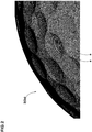
- Fig.2 shows a part of the solid object model 2 which is a closed surface model 2a of a golf ball.
- the surface of the golf ball is modeled with a large number of triangular planar elements (e) which are linked with each other into a spherical shape with dimples.
- the element surface planes (n) planes of the elements (e) which planes collectively define the surface of the solid object model 2 are hereinafter referred as the element surface planes (n). Therefore, in the case of the golf ball model shown in Fig.2 , the element surface plane (n) is a triangle. If quadrilateral elements (e) are used, the element surface plane (n) is a rectangle.
- the solid object model 2 is prepared in the above-mentioned computer 1. This means that data about at least the configuration of the surface of the solid object model 2 are loaded and stored in the storage device of the computer 1.
- the coordinate system mesh 3 is prepared in the computer 1. This means that data about at least the coordinates of the grid points 3a in the basic coordinate system are loaded and stored in the storage device of the computer 1.
- Step S3 a boundary definition processing is performed in order that the boundary between the solid object model 2 and fluid model is defined on coordinate system mesh 3.
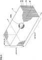
- the coordinate system mesh 3 in this example is an orthogonal mesh M defined in a form of a substantially rectangular parallelepiped which has 3D sizes capable of encompassing the object (golf ball) model 2 completely in order to simulate air flow around the entire surface of the solid object model 2.
- the orthogonal mesh M is divided by a positive integer d1 in x-axis direction, a positive integer d2 in Y-axis direction and a positive integer d3 in Z-axis direction in the X-Y-Z orthogonal coordinate system of the three-dimensional space.
- the grid points 3a are disposed at cross-points of the mesh lines of the orthogonal mesh M.
- the spacings of the mesh lines for example, in the case of a golf ball model 2 having an outer diameter of 42.7mm, it is preferable that the distance between the grid points in X-axis direction, the distance between the grid points in Y-axis direction and the distance between the grid points in X-axis direction are each set in a range of from 0.025 mm to 1.0 mm.
- these distances can be changed, depending on the 3D sizes of the solid object model 2, required analytical accuracy, fluid velocity and the like.
- the 3D sizes and shape of the coordinate system mesh 3 can be changed, depending on the region to be simulated.
- the solid object model 2 is placed in the coordinate system mesh 3 so as to wholly overlap with the coordinate system mesh 3 as shown in Fig.3 .
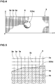
- Fig.5 is a magnified figure of part A of Fig.4 .
- some of the grid points 3a of the coordinate system mesh 3 are positioned inside the solid object model 2 where no flow occurs. Therefore, in performing the fluid simulation, it is necessary to determine which of the grid points 3a are positioned inside the solid object model 2, and accordingly which of the grid points 3a are positioned outside the solid object model 2, and the boundary is defined for the coordinate system mesh 3 so that the coordinate system mesh 3 is separated into a solid region s and a fluid region F to define the fluid model.
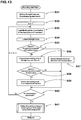
- FIG.13 An example of flow chart of the boundary definition processing performed by the computer 1 is shown in Fig.13 .
- a large number of straight lines L passing through the grid points 3a of the coordinate system mesh 3 are defined (Step S31) so that the straight lines L coincide with the mesh lines constituting the coordinate system mesh 3, and the straight lines L include straight lines L1 parallel with X-axis, straight lines L2 parallel with Y-axis and straight lines L3 parallel with Z-axis. All of the mesh lines respectively have the straight lines L coinciding therewith, therefore, each of the grid points 3a is located on one of the straight lines L1, one of the straight lines L2 and one of the straight lines L3.
- the number of the straight lines L1 is equal to the product of d2 and d3.
- the number of the straight lines L2 is equal to the product of d1 and d3.
- the number of the straight lines L3 is equal to the product of d1 and d2, wherein d1, d2 and d3 are the above-mentioned positive integers. It is however, not always necessary to have all of the mesh lines coincide with the straight lines L. In other words, it is possible some of the mesh lines have no straight line L coinciding therewith as explained later. It is enough for the straight lines L to have finite lengths such that the straight lines L extends across the solid object model completely in the X, Y and Z-axis directions.
- Step S32 This variable h is used as an index number of the above-mentioned element surface plane (n) to be possessed.
- Step S33 the coordinates of the node points of the h-numbered element surface plane (n) are loaded onto the working memory.
- the element (e) is a triangle planar element (e) as shown in Fig.7 .
- the coordinate values of the three node points P1, P2 and P3 defining the element surface plane (n) are loaded onto the working memory.
- a database of the coordinate values of the node points of all of the element surface planes (n) which are indexed by the numbers (h) are prepared and stored in the computer 1 beforehand.
- Step S35 If “Yes” in the Step S35, namely, the current straight line L is parallel with the h-numbered element surface plane (n), then it is decided that the current straight line does not intersect with the h-numbered element surface plane (n). (step S37)
- Step S35 namely, the current straight line L is not parallel with the h-numbered element surface plane (n)
- the intersecting point of the current straight line L with a plane N is computed.
- the plane N is, as shown in Fig.7 , a plane including the h-numbered element surface plane (n).
- the plane N is defined by an equation using the coordinates of the node points (P1-P3) of the h-numbered element surface plane (n).
- the intersecting point of the current straight line L and the plane N relating to the h-numbered element surface plane (n) can be obtained by solving the system of the equation defining the plane N and the equation defining the current straight line L.
- the equation defining the plane N is preferably included in the above-mentioned database together with the coordinate values of the node points for each of the element surface planes (n).
- Step S38 If "Yes” in the Step S38, namely, the intersecting point C is inside the h-numbered element surface plane (n), then the intersecting point is decided and stored as an intersecting point C of the current straight line L with the surface of the object model 2. (Step S39)
- step S41 the boundary between the solid object model 2 and the fluid model is defined on the coordinate system mesh 3.
- the odd-numbered intersecting points are of the intersection from the outside towards the inside of the solid object model 2
- the even-numbered intersecting points are of the intersection from the inside towards the outside of the solid object model 2. Therefore, as shown in Fig.10 . some of the grid points 3a (filled circle) on the straight line L which exist between an odd-numbered intersecting point and an even-numbered intersecting point next thereto are considered and defined as being positioned in the solid region s (inside the solid object model), and the remaining grid points 3a on the straight line L (open circle) are considered and defined as being positioned in the fluid region F (outside the solid object model).
- Step S41 firstly, with respect to each of the straight lines L, it is checked if the straight line L intersects the surface of the solid object model 2. If "Yes", the computer 1 determines and stores the intersecting order of the intersecting points C in a predetermined direction of the straight line L.
- the boundary between the solid region S and fluid region F can be easily located, regardless of whether the configuration of the solid object model 2 is simple or complex.
- the straight lines L include the straight lines L1 parallel with x-axis, the straight lines L2 parallel with Y-axis and the straight lines L3 parallel with Z-axis. Therefore, the above-described processing is performed for the straight lines L1, L2 and L3.
- Fig.11 shows another example of the coordinate system mesh 3 in which a cylindrical coordinate system is employed as the basic coordinate system.
- the coordinate system mesh 3 is a cylindrical Eulerian mesh M which is divided by a positive integer d1 in polar axis direction (r), a positive integer d2 in azimuth direction ( ⁇ ) and a positive integer d3 in cylindrical axis direction (z) in the r- ⁇ -z cylindrical coordinate system.
- the grid points 3a are disposed at cross-points of the mesh lines of the mesh M.
- straight lines L are coincide with the straight mesh lines, therefore, in this example, the straight lines L are
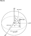
- Fig.12 shows another example of the coordinate system mesh 3 in which a spherical coordinate system is employed as the basic coordinate system.
- the coordinate system mesh 3 is a spherical Eulerian mesh M which is divided by a positive integer d1 in radial direction (r) a positive integer d3 in azimuth angle direction ( ⁇ ) a positive integer d2 in inclination angle direction ( ⁇ ) in the r- ⁇ - ⁇ spherical coordinate system.
- the grid points 3a are disposed at cross-points of the mesh lines of the mesh M.
- the above-mentioned straight lines L are coincide with the straight mesh lines, therefore, in this example, the straight lines L are straight lines L6 extending radially from the origin O of the coordinate system the number of which is equal to the product of d2 and d3.
- Each of the grid points 3a is disposed on one of the straight lines L6. Therefore, the above-described processing is performed for only the straight lines L6. This helps to greatly reduce the computing time.
- the boundary can be defined by using the intersecting points C of the straight lines L with the element surface planes (n) as explained above. Accordingly, in comparison with conventional algorithms which search, in a three-dimensional space, grid points nearest to the node points of elements constituting the surface of the solid object model 2, the computing is simplified and the computing time can be greatly reduced. Further, the grid points 3a on the straight line L falling between the boundary points can be defined as being in the solid region s on the block. Therefore, it is possible to speed up the process of marking the grid points as being positioned in the solid region S.
- the coordinates of the grid points 3a on the straight line L are expressed by one-dimensional coordinate values based on a one-dimensional coordinate system defined along the straight line L, and these one-dimensional coordinate values are used as the above-mentioned set of real numbers x[i].
- a one-dimensional coordinate value of the intersecting point C in the same one-dimensional coordinate system is used.
- the nearest neighbor search method in this example comprises:
- the construction phase S41s is performed only once before the search phase S41b.
- the database for search includes, with respect to each of the straight lines L, a set of real numbers (x[1], x[2], x[3] --- x[n]) corresponding to the above-mentioned one-dimensional coordinate values of the grid points 3a on the straight line L.
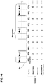
- the database includes a series Br of buckets B per each set of the real numbers (x[1], x[2], x[3] --- x[n]) as shown in Fig.14 .
- the buckets B respectively correspond to small one-dimensional spaces defined by dividing a one-dimensional space between a minimum real number x[1] and a maximum real number x[n] at regular intervals, whereby the number of the buckets B and the number of the small one-dimensional spaces are the same integral number m. Accordingly, each bucket B[j] can be considered as a one-dimensional space between a real number y1 and a real numbers y2, wherein y1 ⁇ y2, and the difference y2 - y1 is constant through all the buckets.
- bucket index A bucket B with a bucket index j is denoted by bucket B[j] (j: 1 to m). Therefore, if one or more of the real numbers x[i] (i: 1 to n) satisfy a condition y1 ⁇ x[i] ⁇ y2 of either one of the buckets B[j] (j: 1 to m), then the one or more of the real numbers are determined as belonging to the bucket, and the bucket comprises data about the one or more of the real numbers.
- Each of the buckets B[j] comprises data about its bucket size.
- the bucket size is the number of the real number(s) x[i] belonging to the bucket B[j] under consideration. In the case that there is no real number belonging to the bucket under consideration, the bucket size is zero, therefore, the bucket comprises such data that the bucket size is zero.
- the buckets B[1], B[2], B[6], B[9] and B[10] each have one real number x[1], x[2], x[3], x[4], x[5], respectively, therefore, the bucket sizes of these buckets B are equal to 1.
- the buckets B[3], B[4], B[5], B[7] and B[8] have no real number, therefore, these buckets comprise date about the bucket sizes being equal to zero.
- Each of the buckets B[j] further comprises data about a bucket index of a last filled bucket ("BIofLFB" for short).
- the last filled bucket is a bucket whose bucket size is not zero and whose bucket index is nearest to the bucket index of the bucket under consideration.
- the computer 1 scans the real numbers x[1] -- x[n] in ascending order, starting from x[1] to x[n], in order to determine if each real number x[i] satisfies a condition y1 ⁇ x[i] ⁇ y2 of either one of the buckets, and thereby to determine which one of the buckets the real number x[i] belongs to.
- the first bucket B[1] its own bucket index, namely, "1" is treated as the BIofLFB, and the first bucket B[1] comprises data about the BIofLFB being 1.
- Each bucket whose bucket size is not zero further, comprises data about the minimum and maximum of the real number(s) belonging to the bucket under consideration.
- the bucket size is "1"
- this single real number is treated as the minimum and maximum real numbers. Namely, the minimum and maximum real numbers are equal to the single real number.
- Fig.15 shows an example of the construction phase S41a, wherein: --
- the central processing unit loads the set of real numbers (x[1], x[2], x[3] --- x[n]) in working memory. (Step S51).
- the central processing unit defines the range (y1 to y2) of each bucket based on the range (x[1] to x[n]) of the real numbers divided by the number m. -- (Step S52)
- the integral number m is set in a range between about 2 times and several times the number n of the real numbers x[1] to x[n].
- the central processing unit allocate main memory for the buckets B[1] to B[m] needed for storing data about the bucket size, the BIofLFB, the real number(s) and the minimum and maximum thereof. (Step S53)
- the central processing unit puts data about the real numbers x[1] to x[n] into the respective buckets in the main memory. -- (step S54)
- Step S54 using the integral number m and the real numbers x[1] and x[n], the spatial size ⁇ x of a bucket is determined by the following expression (1).
- ⁇ ⁇ x x n ⁇ x 1 / m All of the buckets have the same spatial size ⁇ x.
- the central processing unit evaluates the following expression (2).
- ibucket # floor x i ⁇ x 1 / ⁇ x + 1 wherein #floor(y) is a function which returns the largest integral value not greater than y.
- the central processing unit puts data about the real number x[i] into the bucket B[ibucket], and performs the calculation of the following assignment expression (3) in order to increment the bucket size stored in the bucket B[ibucket] by one.
- bucket size bucket size + 1 If need arises as a results of the inclusion of the real number x[i] into the bucket B[ibucket], then the central processing unit updates the minimum real number and/or maximum real number stored in the bucket B[ibucket].
- the database include buckets whose bucket size is zero. Accordingly, it is expedient to exclude such zero-size buckets from the nearest neighbor search.
- the central processing unit determines the BIofLFB, and stores data about the BIofLFB in the bucket B[j]. -- (Step S55)
- This Step S15 is as follows.
- the last filled bucket is a bucket whose bucket size is not zero and whose bucket index is nearest to the bucket under consideration on the first bucket side. Therefore, the last filled bucket is defined by the following conditions (a), (b) and (c):
- Fig.16 shows an example of a sequence of operations by which the central processing unit determines the BIofLFB.
- the central processing unit puts 1 (integral number) into both of a variable LFB and a variable k. -- (step S60, S61)
- the central processing unit determines if the bucket size is more than zero. -- (step S62)
- step S62 if the result is true (Y) (namely, more than zero), then the central processing unit stores the current value of the variable LFB in the bucket B[var.k] as the date about the BIofLFB. -- (step S63)
- the central processing unit updates the variable LFB to be equal to the bucket index of the current bucket B[var.k]. --(step S64) Then the sequence goes to Step s65.
- Step S62 if the result is false (No) (namely, equal to zero), then the central processing unit stores the current value of the variable LFB in the bucket B[var.k] as the date about the BIofLFB. -- (step S66)
- step S65 without updating or changing the variable LFB.
- the central processing unit checks if the variable k which is the bucket index of the current bucket is equal to the bucket index of the last bucket (namely, m).
- step S67 the central processing unit increments the variable k by one (step S67), and the sequence goes to the step S62. These steps are repeated till the last bucket B[m].
- the database for used in the search phase S41b is prepared. Such construction phase is performed only once before the search phase S41b.
- the main memory is faster in the access speed than the storage device, therefore, the database is allocated on the main memory. It is however also possible to allocate the database on the storage device.
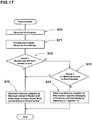
- Fig.17 shows an example of a sequence of operations by which the central processing unit determines the nearest neighbor.
- the central processing unit determines the bucket index "ibucket" of a bucket which the query point q belongs to.-(step S71)
- ibucket # floor q ⁇ x 1 / ⁇ x + 1 wherein, #floor(y) is a function which returns the largest integral value not greater than y.
- the central processing unit checks if the bucket size of the bucket B[ibucket] is zero. -- (step S72)
- step S72 if the result is false (No) (namely, bucket size > 0), then the central processing unit searches the real number(s) belonging to or contained in the bucket B[ibucket] for the nearest neighbor. -- (step S73, step S74)
- the central processing unit compares the query point q with the minimum real number stored in the bucket B[ibucket].
- Step S73 If the query point q is less than the minimum real number (in the Step S73, Yes), then it is determined that the nearest neighbor is the maximum real number stored in the last filled bucket whose bucket index is stored in the bucket B[ibucket]. -- (Step S75)
- the whole search is performed on one of the buckets during the subsequent steps to the step S72. Therefore, the nearest neighbor can be found very quickly, and the computing time can be greatly decreased.
- a real number not more than the query point q and nearest to the query point q is found as the nearest neighbor.
- the solid object model was a closed surface model of a golf ball, wherein the radius was 21.35 mm, and only the surface was modeled with rigid triangular planar Lagrangian elements, and the total number of the node points was 3,755,598.
- the coordinate system mesh was a cylindrical mesh based on a cylindrical coordinate system (r, ⁇ ,z), wherein the radius was 220 mm, the size in the cylindrical axis direction was 440 mm, the division numbers, namely, the above-mentioned positive integers d1 in polar axis direction (r), positive integer d2 in azimuth direction ( ⁇ ) and positive integer d3 in cylindrical axis direction (z) were as follows.
- ANN program Nearest neighbor search program
- Embodiment In order to define the boundary points, the method as claimed in claim 1 was used. As to the method to mark up or define grid points as positioned in the solid region, grid points on each straight line existing between the boundary points were marked up on the block.
Landscapes
- Engineering & Computer Science (AREA)
- Physics & Mathematics (AREA)
- Theoretical Computer Science (AREA)
- Computer Hardware Design (AREA)
- Evolutionary Computation (AREA)
- Geometry (AREA)
- General Engineering & Computer Science (AREA)
- General Physics & Mathematics (AREA)
- Management, Administration, Business Operations System, And Electronic Commerce (AREA)
Claims (5)
- Verfahren zum Verkürzen der Grenzendefinitionsdauer und der Festkörpermarkierungszeit zum Definieren einer Fluid/Festkörper-Grenze, wobei das Verfahren zur computergestützten Fluiddynamiksimulation Gebrauch macht von
einem Koordinatensystem-Netz, das einen Bereich eines dreidimensionalen Raums, der einen Fluidbereich einschließt, modelliert und das durch eine große Zahl von in dem Bereich des dreidimensionalen Raums angeordneten Gitterpunkten definiert ist, und
einem Festkörperobjektmodell, das ein Festkörperobjekt modelliert und dessen Oberfläche aus Ebenen von endlichen Elementen besteht, wobei
das Festkörperobjektmodell eine Mischvorrichtung modelliert und das Koordinatensystem-Netz die Strömung von Verbundwerkstoffen in der Mischvorrichtung modelliert,
wobei das Verfahren umfasst
einen Schritt (a) eines Erstellens des Festkörperobjektmodells in einem Computer,
einen Schritt (b) eines Erstellens des Koordinatensystem-Netzes in dem Computer,
einen Schritt (c), in dem Computer, eines Definierens von geraden Linien, die sich über den oben genannten Bereich des dreidimensionalen Raumes erstrecken und durch die Gitterpunkte verlaufen,
einen Schritt (d), der von dem Computer ausgeführt wird, eines Beschaffens von Schnittpunkten der geraden Linien mit der Oberfläche des Festkörperobjektmodells,
einen Schritt (e), der von dem Computer ausgeführt wird, in welchem für jede der geraden Linien, die die Schnittpunkte aufweisen,
die auf der geraden Linie positionierten Gitterpunkte nach einem nächstgelegenen Gitterpunkt zu jedem der Schnittpunkte durchsucht werden und basierend auf den herausgesuchten nächstgelegenen Gitterpunkten, die auf jeder der geraden Linien positionierten Gitterpunkte jeweils dahingehend bestimmt werden, ob der Gitterpunkt innerhalb des Festkörperobjektmodells oder in dem Fluidbereich positioniert ist, wodurch alle in dem Bereich des dreidimensionalen Raumes angeordneten Gitterpunkte dahingehend bestimmt werden, ob der Gitterpunkt in dem Fluidbereich oder innerhalb des Festkörperobjektmodells positioniert ist und dadurch
die Grenze zwischen dem Festkörperobjektkörpermodell und dem Fluidbereich auf dem Koordinatensystem-Netz definiert wird. - Verfahren nach Anspruch 1, wobei
das Koordinatensystem-Netz basierend auf einem orthogonalen X-Y-Z-Koordinatensystem definiert wird, so dass es gerade Netzlinien aufweist, die sich in der X-Achsenrichtung, der Y-Achsenrichtung und der Z-Achsenrichtung erstrecken,
die Gitterpunkte auf den geraden Netzlinien positioniert werden, und
die geraden Linien so definiert werden, dass sie mit den geraden Netzlinien übereinstimmen. - Verfahren nach Anspruch 1, wobei
das Koordinatensystem-Netz basierend auf einem zylindrischen r-θ-z-Koordinatensystem definiert wird, so dass es gerade Netzlinien aufweist, die sich in den Richtungen der Zylinderachse z und der Polarachse r erstrecken,
die Gitterpunkte auf den geraden Netzlinien positioniert werden, und
die geraden Linien so definiert werden, dass sie mit den geraden Netzlinien übereinstimmen. - Verfahren nach Anspruch 1, wobei
das Koordinatensystem-Netz basierend auf einem r-θ-ø-Kugelkoor-dinatensystem definiert wird, so dass es gerade Netzlinien aufweist, die sich in Richtungen der Polarachse r erstrecken,
die Gitterpunkte auf den geraden Netzlinien positioniert werden, und
die geraden Linien so definiert werden, dass sie mit den geraden Netzlinien übereinstimmen. - Verfahren nach Anspruch 1, wobei
in dem Suchprozess in dem Schritt (e), der für jede der geraden Linie mit den Schnittpunkten durchgeführt wird, um die auf der geraden Linie positionierten Gitterpunkte nach einem nächsten Punkt zu jedem der Schnittpunkte zu durchsuchen,
die Koordinaten der auf der geraden Linie positionierten Gitterpunkte betrachtet und deren Schnittpunkte als eindimensionale Werte basierend auf einem entlang der geraden Linie definierten eindimensionalen Koordinatensystem genommen werden, und
wenn die eindimensionalen Koordinatenwerte der Gitterpunkte als eine Menge von reellen Zahlen x[i] (i: 1 bis n) gegeben sind, und
die eindimensionalen Koordinatenwerte eines jeden der Schnittpunkte als Abfragepunkt q gegeben sind,
die Durchsuchung der Gitterpunkte nach einem nächstgelegenen Punkt zu jedem der Schnittpunkte durch ein Suchverfahren für nächstgelegene Nachbarn durchgeführt wird, umfassend
eine Konstruktionsphase, in der eine Datenbank der reellen Zahlen x[i] (i: ganze Zahlen von 1 bis n, die in aufsteigender Reihenfolge der reellen Zahlen zugeordnet sind) in einem Speicher des Computers erstellt wird, und
eine Suchphase, in der der Computer den nächsten Nachbarn zu dem Abfragepunkt q unter Verwendung der Datenbank sucht, wobei
die Datenbank eine Reihe von Buckets umfasst,
die Buckets jeweils kleinen eindimensionalen Räumen entsprechen, die definiert sind, indem ein eindimensionaler Raum in regelmäßigen Intervallen zwischen einer minimalen reellen Zahl x[1] und einer maximalen reellen Zahl x[n] geteilt wird, wodurch die Zahl der Buckets und die Zahl der kleinen eindimensionalen Räume die gleiche ganzzahlige Zahl m ist,
die Buckets eindeutige Bucket-Indizes von dem ersten Bucket B[1] bis zum letzten Bucket B[m] haben,
jeder der Buckets Daten über reelle(n) Zahl(en) umfasst, die in einen der kleinen eindimensionalen Räume fallen, der dem betrachteten Bucket entspricht,
jeder der Buckets ferner Daten über seine Bucket-Größe umfasst, wobei die Bucket-Größe durch die Zahl der reellen Zahl(en) definiert ist, die in einen der kleinen eindimensionalen Räume fallen, der dem betrachteten Bucket entspricht,
jeder der Buckets mit Ausnahme der ersten Buckets B[1] ferner Daten über den Bucket-Index eines zuletzt gefüllten Buckets umfasst, wobei der zuletzt gefüllte Bucket als Bucket definiert ist, dessen Bucket-Größe nicht Null ist und dessen Bucket-Index dem des betrachteten Buckets am nächsten liegt, und
die Suchphase, die umfasst:einen ersten Schritt eines Lokalisierens eines der Buckets, der einem der kleinen eindimensionalen Räume entspricht, in den der Abfragepunkt q fällt,einen zweiten Schritt eines Überprüfens der Bucket-Größe des lokalisierten Buckets, ob dessen Bucket-Größe Null ist oder nicht,einen dritten Schritt einer Suche nach dem nächstgelegenen Nachbarn unter Verwendung der Daten der realen Zahl(en), die enthalten sind in- dem lokalisierten Bucket, wenn die geprüfte Bucket-Größe nicht Null ist,
oder- einem Bucket mit einem Bucket-Index, der gleich dem Bucket-Index des zuletzt gefüllten Buckets ist, der in dem lokalisierten Bucket enthalten ist, wenn die geprüfte Bucket-Größe Null ist.
Applications Claiming Priority (1)
| Application Number | Priority Date | Filing Date | Title |
|---|---|---|---|
| JP2010082785A JP5033211B2 (ja) | 2010-03-31 | 2010-03-31 | 流体シミュレーションにおける境界位置決定方法 |
Publications (2)
| Publication Number | Publication Date |
|---|---|
| EP2372585A1 EP2372585A1 (de) | 2011-10-05 |
| EP2372585B1 true EP2372585B1 (de) | 2019-08-14 |
Family
ID=43923779
Family Applications (1)
| Application Number | Title | Priority Date | Filing Date |
|---|---|---|---|
| EP10015740.3A Not-in-force EP2372585B1 (de) | 2010-03-31 | 2010-12-16 | Verfahren zur Definierung einer Flüssigkeits-/Feststoffoberfläche für numerische Strömungssimulationen |
Country Status (3)
| Country | Link |
|---|---|
| US (1) | US8797316B2 (de) |
| EP (1) | EP2372585B1 (de) |
| JP (1) | JP5033211B2 (de) |
Families Citing this family (10)
| Publication number | Priority date | Publication date | Assignee | Title |
|---|---|---|---|---|
| JP5227384B2 (ja) * | 2010-10-12 | 2013-07-03 | 住友ゴム工業株式会社 | 構造格子を用いたシミュレーション方法 |
| JP5750091B2 (ja) * | 2012-11-16 | 2015-07-15 | 住友ゴム工業株式会社 | 流体シミュレーション方法 |
| US9984039B2 (en) * | 2014-09-25 | 2018-05-29 | International Business Machines Corporation | Domain decomposition for transport trajectories in advection diffusion processes |
| CN111368380B (zh) * | 2018-12-24 | 2022-07-26 | 中国空气动力研究与发展中心超高速空气动力研究所 | 一种用于n-s/dsmc耦合算法的区域边界优化方法 |
| CN115600316B (zh) * | 2022-10-17 | 2023-05-12 | 中国船舶科学研究中心 | 一种船底气液分层两相流波动形态数值模拟方法 |
| CN115880670B (zh) * | 2022-12-14 | 2025-06-20 | 长三角哈特机器人产业技术研究院 | 图像中的三角形检测方法及停车位检测系统 |
| CN116151084B (zh) * | 2023-04-21 | 2023-07-14 | 中国空气动力研究与发展中心计算空气动力研究所 | 基于结构网格的模拟方法、装置、终端设备及存储介质 |
| CN116229021B (zh) * | 2023-05-08 | 2023-08-25 | 中国空气动力研究与发展中心计算空气动力研究所 | 一种浸没边界虚拟网格嵌入方法、装置、设备及介质 |
| CN117451769B (zh) * | 2023-12-19 | 2024-03-15 | 四川省水利科学研究院 | 一种堆石混凝土施工质量检测方法 |
| CN118938692B (zh) * | 2024-10-15 | 2024-12-17 | 贵州健易测科技有限公司 | 基于物联网的刺梨鲜果保鲜环境智能调控方法及其系统 |
Family Cites Families (14)
| Publication number | Priority date | Publication date | Assignee | Title |
|---|---|---|---|---|
| JPH01106266A (ja) * | 1987-10-20 | 1989-04-24 | Matsushita Electric Ind Co Ltd | 3次元図形処理方法およびその装置 |
| JPH01304588A (ja) * | 1988-06-01 | 1989-12-08 | Oki Electric Ind Co Ltd | クリッピング処理方式 |
| JPH04127379A (ja) * | 1990-09-19 | 1992-04-28 | Babcock Hitachi Kk | 解析対象物の要素分割方法およびその装置 |
| JP3265879B2 (ja) * | 1994-11-25 | 2002-03-18 | 日産自動車株式会社 | 3次元直交格子データの生成装置 |
| JPH1125293A (ja) * | 1997-07-02 | 1999-01-29 | Hitachi Ltd | メッシュ生成方法 |
| JP4308465B2 (ja) * | 2000-12-12 | 2009-08-05 | 富士通株式会社 | 連成解析方法、その解析条件設定方法、その記憶媒体及びそのプログラム |
| JP3626113B2 (ja) * | 2001-05-31 | 2005-03-02 | 住友ゴム工業株式会社 | 気体流シミュレーション方法 |
| JP2003085569A (ja) * | 2001-09-14 | 2003-03-20 | Canon Inc | 内外点判定アルゴリズム |
| JP3978534B2 (ja) * | 2001-11-16 | 2007-09-19 | 独立行政法人理化学研究所 | 固定格子上を移動する移動境界の設定方法およびそれを実現するコンピュータプログラム |
| JP2004145719A (ja) * | 2002-10-25 | 2004-05-20 | Hitachi Ltd | 数値解析における境界条件設定方法、境界条件設定システム及び境界条件設定プログラム並びに媒体 |
| US7239990B2 (en) * | 2003-02-20 | 2007-07-03 | Robert Struijs | Method for the numerical simulation of a physical phenomenon with a preferential direction |
| JP4783100B2 (ja) * | 2005-09-12 | 2011-09-28 | 独立行政法人理化学研究所 | 境界データのセル内形状データへの変換方法とその変換プログラム |
| US7921002B2 (en) * | 2007-01-04 | 2011-04-05 | Honda Motor Co., Ltd. | Method and system for simulating flow of fluid around a body |
| JP5333815B2 (ja) * | 2008-02-19 | 2013-11-06 | 株式会社日立製作所 | k最近傍検索方法、k最近傍検索プログラム及びk最近傍検索装置 |
-
2010
- 2010-03-31 JP JP2010082785A patent/JP5033211B2/ja not_active Expired - Fee Related
- 2010-12-13 US US12/966,393 patent/US8797316B2/en active Active
- 2010-12-16 EP EP10015740.3A patent/EP2372585B1/de not_active Not-in-force
Non-Patent Citations (1)
| Title |
|---|
| None * |
Also Published As
| Publication number | Publication date |
|---|---|
| JP2011215823A (ja) | 2011-10-27 |
| EP2372585A1 (de) | 2011-10-05 |
| US8797316B2 (en) | 2014-08-05 |
| US20110242095A1 (en) | 2011-10-06 |
| JP5033211B2 (ja) | 2012-09-26 |
Similar Documents
| Publication | Publication Date | Title |
|---|---|---|
| EP2372585B1 (de) | Verfahren zur Definierung einer Flüssigkeits-/Feststoffoberfläche für numerische Strömungssimulationen | |
| US10460062B2 (en) | Method and computer program for determining a placement of at least one circuit for a reconfigurable logic device | |
| US5289567A (en) | Computer apparatus and method for finite element identification in interactive modeling | |
| US11120191B2 (en) | Multi-tier co-placement for integrated circuitry | |
| KR100537574B1 (ko) | 그래픽 이미지 생성 장치, 생성 방법 및 그 프로그램을 기록한 컴퓨터 판독 가능한 기록매체 | |
| KR20130098306A (ko) | 계산용 데이터 생성 장치, 계산용 데이터 생성 방법 및 계산용 데이터 생성 프로그램 | |
| WO2011076908A2 (en) | An improved computer-implemented method of geometric feature detection | |
| JP2012074000A (ja) | 有限要素法を用いた解析方法、及び有限要素法を用いた解析演算プログラム | |
| JP5644606B2 (ja) | メッシュ数予測方法、解析装置及びプログラム | |
| CN115630542B (zh) | 一种薄壁加筋结构的加筋布局优化方法 | |
| Cascón et al. | Comparison of the meccano method with standard mesh generation techniques | |
| CN111222221A (zh) | 制造运动物品的至少一部分的方法 | |
| US8484605B2 (en) | Analysis of physical systems via model libraries thereof | |
| Schmidt et al. | Extended isogeometric analysis of multi-material and multi-physics problems using hierarchical B-splines | |
| Torres et al. | Convex polygon packing based meshing algorithm for modeling of rock and porous media | |
| CN115049176A (zh) | 材料性能评估方法、装置及计算机设备 | |
| WO2021161503A1 (ja) | 設計プログラムおよび設計方法 | |
| Serpa et al. | Flexible use of temporal and spatial reasoning for fast and scalable CPU broad‐phase collision detection using KD‐Trees | |
| Haunert et al. | Propagating updates between linked datasets of different scales | |
| Daviet et al. | Neurally integrated finite elements for differentiable elasticity on evolving domains | |
| Marco et al. | Structural shape optimization using Cartesian grids and automatic h-adaptive mesh projection | |
| US8271518B2 (en) | Nearest neighbor search method | |
| US10830594B2 (en) | Updating missing attributes in navigational map data via polyline geometry matching | |
| Spira et al. | Hardware acceleration of gate array layout | |
| CN114662009A (zh) | 一种基于图卷积的工业互联网工厂协同推荐算法 |
Legal Events
| Date | Code | Title | Description |
|---|---|---|---|
| PUAI | Public reference made under article 153(3) epc to a published international application that has entered the european phase |
Free format text: ORIGINAL CODE: 0009012 |
|
| AK | Designated contracting states |
Kind code of ref document: A1 Designated state(s): AL AT BE BG CH CY CZ DE DK EE ES FI FR GB GR HR HU IE IS IT LI LT LU LV MC MK MT NL NO PL PT RO RS SE SI SK SM TR |
|
| AX | Request for extension of the european patent |
Extension state: BA ME |
|
| 17P | Request for examination filed |
Effective date: 20120118 |
|
| STAA | Information on the status of an ep patent application or granted ep patent |
Free format text: STATUS: EXAMINATION IS IN PROGRESS |
|
| 17Q | First examination report despatched |
Effective date: 20170222 |
|
| GRAP | Despatch of communication of intention to grant a patent |
Free format text: ORIGINAL CODE: EPIDOSNIGR1 |
|
| STAA | Information on the status of an ep patent application or granted ep patent |
Free format text: STATUS: GRANT OF PATENT IS INTENDED |
|
| INTG | Intention to grant announced |
Effective date: 20190225 |
|
| GRAS | Grant fee paid |
Free format text: ORIGINAL CODE: EPIDOSNIGR3 |
|
| GRAA | (expected) grant |
Free format text: ORIGINAL CODE: 0009210 |
|
| STAA | Information on the status of an ep patent application or granted ep patent |
Free format text: STATUS: THE PATENT HAS BEEN GRANTED |
|
| AK | Designated contracting states |
Kind code of ref document: B1 Designated state(s): AL AT BE BG CH CY CZ DE DK EE ES FI FR GB GR HR HU IE IS IT LI LT LU LV MC MK MT NL NO PL PT RO RS SE SI SK SM TR |
|
| REG | Reference to a national code |
Ref country code: GB Ref legal event code: FG4D |
|
| REG | Reference to a national code |
Ref country code: CH Ref legal event code: EP Ref country code: AT Ref legal event code: REF Ref document number: 1167864 Country of ref document: AT Kind code of ref document: T Effective date: 20190815 |
|
| REG | Reference to a national code |
Ref country code: IE Ref legal event code: FG4D |
|
| REG | Reference to a national code |
Ref country code: DE Ref legal event code: R096 Ref document number: 602010060516 Country of ref document: DE |
|
| REG | Reference to a national code |
Ref country code: DE Ref legal event code: R079 Ref document number: 602010060516 Country of ref document: DE Free format text: PREVIOUS MAIN CLASS: G06F0017500000 Ipc: G06F0030000000 |
|
| REG | Reference to a national code |
Ref country code: NL Ref legal event code: MP Effective date: 20190814 |
|
| REG | Reference to a national code |
Ref country code: LT Ref legal event code: MG4D |
|
| PG25 | Lapsed in a contracting state [announced via postgrant information from national office to epo] |
Ref country code: FI Free format text: LAPSE BECAUSE OF FAILURE TO SUBMIT A TRANSLATION OF THE DESCRIPTION OR TO PAY THE FEE WITHIN THE PRESCRIBED TIME-LIMIT Effective date: 20190814 Ref country code: PT Free format text: LAPSE BECAUSE OF FAILURE TO SUBMIT A TRANSLATION OF THE DESCRIPTION OR TO PAY THE FEE WITHIN THE PRESCRIBED TIME-LIMIT Effective date: 20191216 Ref country code: SE Free format text: LAPSE BECAUSE OF FAILURE TO SUBMIT A TRANSLATION OF THE DESCRIPTION OR TO PAY THE FEE WITHIN THE PRESCRIBED TIME-LIMIT Effective date: 20190814 Ref country code: HR Free format text: LAPSE BECAUSE OF FAILURE TO SUBMIT A TRANSLATION OF THE DESCRIPTION OR TO PAY THE FEE WITHIN THE PRESCRIBED TIME-LIMIT Effective date: 20190814 Ref country code: NL Free format text: LAPSE BECAUSE OF FAILURE TO SUBMIT A TRANSLATION OF THE DESCRIPTION OR TO PAY THE FEE WITHIN THE PRESCRIBED TIME-LIMIT Effective date: 20190814 Ref country code: LT Free format text: LAPSE BECAUSE OF FAILURE TO SUBMIT A TRANSLATION OF THE DESCRIPTION OR TO PAY THE FEE WITHIN THE PRESCRIBED TIME-LIMIT Effective date: 20190814 Ref country code: NO Free format text: LAPSE BECAUSE OF FAILURE TO SUBMIT A TRANSLATION OF THE DESCRIPTION OR TO PAY THE FEE WITHIN THE PRESCRIBED TIME-LIMIT Effective date: 20191114 Ref country code: BG Free format text: LAPSE BECAUSE OF FAILURE TO SUBMIT A TRANSLATION OF THE DESCRIPTION OR TO PAY THE FEE WITHIN THE PRESCRIBED TIME-LIMIT Effective date: 20191114 |
|
| REG | Reference to a national code |
Ref country code: AT Ref legal event code: MK05 Ref document number: 1167864 Country of ref document: AT Kind code of ref document: T Effective date: 20190814 |
|
| PG25 | Lapsed in a contracting state [announced via postgrant information from national office to epo] |
Ref country code: ES Free format text: LAPSE BECAUSE OF FAILURE TO SUBMIT A TRANSLATION OF THE DESCRIPTION OR TO PAY THE FEE WITHIN THE PRESCRIBED TIME-LIMIT Effective date: 20190814 Ref country code: RS Free format text: LAPSE BECAUSE OF FAILURE TO SUBMIT A TRANSLATION OF THE DESCRIPTION OR TO PAY THE FEE WITHIN THE PRESCRIBED TIME-LIMIT Effective date: 20190814 Ref country code: IS Free format text: LAPSE BECAUSE OF FAILURE TO SUBMIT A TRANSLATION OF THE DESCRIPTION OR TO PAY THE FEE WITHIN THE PRESCRIBED TIME-LIMIT Effective date: 20191214 Ref country code: LV Free format text: LAPSE BECAUSE OF FAILURE TO SUBMIT A TRANSLATION OF THE DESCRIPTION OR TO PAY THE FEE WITHIN THE PRESCRIBED TIME-LIMIT Effective date: 20190814 Ref country code: AL Free format text: LAPSE BECAUSE OF FAILURE TO SUBMIT A TRANSLATION OF THE DESCRIPTION OR TO PAY THE FEE WITHIN THE PRESCRIBED TIME-LIMIT Effective date: 20190814 Ref country code: GR Free format text: LAPSE BECAUSE OF FAILURE TO SUBMIT A TRANSLATION OF THE DESCRIPTION OR TO PAY THE FEE WITHIN THE PRESCRIBED TIME-LIMIT Effective date: 20191115 |
|
| PG25 | Lapsed in a contracting state [announced via postgrant information from national office to epo] |
Ref country code: TR Free format text: LAPSE BECAUSE OF FAILURE TO SUBMIT A TRANSLATION OF THE DESCRIPTION OR TO PAY THE FEE WITHIN THE PRESCRIBED TIME-LIMIT Effective date: 20190814 |
|
| PG25 | Lapsed in a contracting state [announced via postgrant information from national office to epo] |
Ref country code: RO Free format text: LAPSE BECAUSE OF FAILURE TO SUBMIT A TRANSLATION OF THE DESCRIPTION OR TO PAY THE FEE WITHIN THE PRESCRIBED TIME-LIMIT Effective date: 20190814 Ref country code: IT Free format text: LAPSE BECAUSE OF FAILURE TO SUBMIT A TRANSLATION OF THE DESCRIPTION OR TO PAY THE FEE WITHIN THE PRESCRIBED TIME-LIMIT Effective date: 20190814 Ref country code: DK Free format text: LAPSE BECAUSE OF FAILURE TO SUBMIT A TRANSLATION OF THE DESCRIPTION OR TO PAY THE FEE WITHIN THE PRESCRIBED TIME-LIMIT Effective date: 20190814 Ref country code: PL Free format text: LAPSE BECAUSE OF FAILURE TO SUBMIT A TRANSLATION OF THE DESCRIPTION OR TO PAY THE FEE WITHIN THE PRESCRIBED TIME-LIMIT Effective date: 20190814 Ref country code: EE Free format text: LAPSE BECAUSE OF FAILURE TO SUBMIT A TRANSLATION OF THE DESCRIPTION OR TO PAY THE FEE WITHIN THE PRESCRIBED TIME-LIMIT Effective date: 20190814 Ref country code: AT Free format text: LAPSE BECAUSE OF FAILURE TO SUBMIT A TRANSLATION OF THE DESCRIPTION OR TO PAY THE FEE WITHIN THE PRESCRIBED TIME-LIMIT Effective date: 20190814 |
|
| PG25 | Lapsed in a contracting state [announced via postgrant information from national office to epo] |
Ref country code: CZ Free format text: LAPSE BECAUSE OF FAILURE TO SUBMIT A TRANSLATION OF THE DESCRIPTION OR TO PAY THE FEE WITHIN THE PRESCRIBED TIME-LIMIT Effective date: 20190814 Ref country code: SK Free format text: LAPSE BECAUSE OF FAILURE TO SUBMIT A TRANSLATION OF THE DESCRIPTION OR TO PAY THE FEE WITHIN THE PRESCRIBED TIME-LIMIT Effective date: 20190814 Ref country code: SM Free format text: LAPSE BECAUSE OF FAILURE TO SUBMIT A TRANSLATION OF THE DESCRIPTION OR TO PAY THE FEE WITHIN THE PRESCRIBED TIME-LIMIT Effective date: 20190814 Ref country code: IS Free format text: LAPSE BECAUSE OF FAILURE TO SUBMIT A TRANSLATION OF THE DESCRIPTION OR TO PAY THE FEE WITHIN THE PRESCRIBED TIME-LIMIT Effective date: 20200224 |
|
| REG | Reference to a national code |
Ref country code: DE Ref legal event code: R097 Ref document number: 602010060516 Country of ref document: DE |
|
| PLBE | No opposition filed within time limit |
Free format text: ORIGINAL CODE: 0009261 |
|
| STAA | Information on the status of an ep patent application or granted ep patent |
Free format text: STATUS: NO OPPOSITION FILED WITHIN TIME LIMIT |
|
| PG2D | Information on lapse in contracting state deleted |
Ref country code: IS |
|
| REG | Reference to a national code |
Ref country code: CH Ref legal event code: PL |
|
| 26N | No opposition filed |
Effective date: 20200603 |
|
| REG | Reference to a national code |
Ref country code: BE Ref legal event code: MM Effective date: 20191231 |
|
| PG25 | Lapsed in a contracting state [announced via postgrant information from national office to epo] |
Ref country code: MC Free format text: LAPSE BECAUSE OF FAILURE TO SUBMIT A TRANSLATION OF THE DESCRIPTION OR TO PAY THE FEE WITHIN THE PRESCRIBED TIME-LIMIT Effective date: 20190814 Ref country code: SI Free format text: LAPSE BECAUSE OF FAILURE TO SUBMIT A TRANSLATION OF THE DESCRIPTION OR TO PAY THE FEE WITHIN THE PRESCRIBED TIME-LIMIT Effective date: 20190814 |
|
| PG25 | Lapsed in a contracting state [announced via postgrant information from national office to epo] |
Ref country code: LU Free format text: LAPSE BECAUSE OF NON-PAYMENT OF DUE FEES Effective date: 20191216 Ref country code: IE Free format text: LAPSE BECAUSE OF NON-PAYMENT OF DUE FEES Effective date: 20191216 |
|
| PG25 | Lapsed in a contracting state [announced via postgrant information from national office to epo] |
Ref country code: CH Free format text: LAPSE BECAUSE OF NON-PAYMENT OF DUE FEES Effective date: 20191231 Ref country code: LI Free format text: LAPSE BECAUSE OF NON-PAYMENT OF DUE FEES Effective date: 20191231 Ref country code: BE Free format text: LAPSE BECAUSE OF NON-PAYMENT OF DUE FEES Effective date: 20191231 |
|
| PGFP | Annual fee paid to national office [announced via postgrant information from national office to epo] |
Ref country code: FR Payment date: 20201112 Year of fee payment: 11 Ref country code: GB Payment date: 20201210 Year of fee payment: 11 Ref country code: DE Payment date: 20201201 Year of fee payment: 11 |
|
| PG25 | Lapsed in a contracting state [announced via postgrant information from national office to epo] |
Ref country code: CY Free format text: LAPSE BECAUSE OF FAILURE TO SUBMIT A TRANSLATION OF THE DESCRIPTION OR TO PAY THE FEE WITHIN THE PRESCRIBED TIME-LIMIT Effective date: 20190814 |
|
| PG25 | Lapsed in a contracting state [announced via postgrant information from national office to epo] |
Ref country code: MT Free format text: LAPSE BECAUSE OF FAILURE TO SUBMIT A TRANSLATION OF THE DESCRIPTION OR TO PAY THE FEE WITHIN THE PRESCRIBED TIME-LIMIT Effective date: 20190814 Ref country code: HU Free format text: LAPSE BECAUSE OF FAILURE TO SUBMIT A TRANSLATION OF THE DESCRIPTION OR TO PAY THE FEE WITHIN THE PRESCRIBED TIME-LIMIT; INVALID AB INITIO Effective date: 20101216 |
|
| PG25 | Lapsed in a contracting state [announced via postgrant information from national office to epo] |
Ref country code: MK Free format text: LAPSE BECAUSE OF FAILURE TO SUBMIT A TRANSLATION OF THE DESCRIPTION OR TO PAY THE FEE WITHIN THE PRESCRIBED TIME-LIMIT Effective date: 20190814 |
|
| REG | Reference to a national code |
Ref country code: DE Ref legal event code: R119 Ref document number: 602010060516 Country of ref document: DE |
|
| GBPC | Gb: european patent ceased through non-payment of renewal fee |
Effective date: 20211216 |
|
| PG25 | Lapsed in a contracting state [announced via postgrant information from national office to epo] |
Ref country code: GB Free format text: LAPSE BECAUSE OF NON-PAYMENT OF DUE FEES Effective date: 20211216 Ref country code: DE Free format text: LAPSE BECAUSE OF NON-PAYMENT OF DUE FEES Effective date: 20220701 |
|
| PG25 | Lapsed in a contracting state [announced via postgrant information from national office to epo] |
Ref country code: FR Free format text: LAPSE BECAUSE OF NON-PAYMENT OF DUE FEES Effective date: 20211231 |