EP1217438B1 - Stéréolithographie avec plusieurs types de balayage vectoriel - Google Patents
Stéréolithographie avec plusieurs types de balayage vectoriel Download PDFInfo
- Publication number
- EP1217438B1 EP1217438B1 EP02075796A EP02075796A EP1217438B1 EP 1217438 B1 EP1217438 B1 EP 1217438B1 EP 02075796 A EP02075796 A EP 02075796A EP 02075796 A EP02075796 A EP 02075796A EP 1217438 B1 EP1217438 B1 EP 1217438B1
- Authority
- EP
- European Patent Office
- Prior art keywords
- layer
- vectors
- flat
- hatch
- facing
- Prior art date
- Legal status (The legal status is an assumption and is not a legal conclusion. Google has not performed a legal analysis and makes no representation as to the accuracy of the status listed.)
- Expired - Lifetime
Links
- 239000013598 vector Substances 0.000 title claims description 1215
- 238000000034 method Methods 0.000 claims description 500
- 238000004519 manufacturing process Methods 0.000 claims description 48
- 238000012545 processing Methods 0.000 claims description 43
- 239000012530 fluid Substances 0.000 claims description 36
- 238000007598 dipping method Methods 0.000 claims description 33
- 230000000638 stimulation Effects 0.000 claims description 18
- 230000015572 biosynthetic process Effects 0.000 claims description 10
- 239000010410 layer Substances 0.000 description 1012
- 238000011960 computer-aided design Methods 0.000 description 338
- 230000008569 process Effects 0.000 description 273
- 229920005989 resin Polymers 0.000 description 174
- 239000011347 resin Substances 0.000 description 174
- 239000007788 liquid Substances 0.000 description 145
- 239000007787 solid Substances 0.000 description 112
- 238000013461 design Methods 0.000 description 105
- 238000004422 calculation algorithm Methods 0.000 description 96
- 239000000463 material Substances 0.000 description 93
- 239000004033 plastic Substances 0.000 description 87
- 229920003023 plastic Polymers 0.000 description 87
- 229920000642 polymer Polymers 0.000 description 59
- 238000001723 curing Methods 0.000 description 57
- 230000033001 locomotion Effects 0.000 description 57
- 230000012447 hatching Effects 0.000 description 51
- 230000008859 change Effects 0.000 description 40
- 238000012546 transfer Methods 0.000 description 40
- OKKJLVBELUTLKV-UHFFFAOYSA-N Methanol Chemical compound OC OKKJLVBELUTLKV-UHFFFAOYSA-N 0.000 description 39
- 238000012937 correction Methods 0.000 description 39
- 230000004044 response Effects 0.000 description 37
- 230000003287 optical effect Effects 0.000 description 35
- 238000006243 chemical reaction Methods 0.000 description 34
- 238000010586 diagram Methods 0.000 description 31
- 238000013459 approach Methods 0.000 description 29
- 238000012423 maintenance Methods 0.000 description 29
- 239000000126 substance Substances 0.000 description 24
- 230000006870 function Effects 0.000 description 22
- 238000006116 polymerization reaction Methods 0.000 description 22
- 230000000694 effects Effects 0.000 description 21
- 230000008901 benefit Effects 0.000 description 20
- 238000012360 testing method Methods 0.000 description 20
- 238000013024 troubleshooting Methods 0.000 description 19
- 238000012805 post-processing Methods 0.000 description 18
- 230000001419 dependent effect Effects 0.000 description 17
- 238000005259 measurement Methods 0.000 description 17
- 239000011343 solid material Substances 0.000 description 17
- 238000004140 cleaning Methods 0.000 description 16
- 238000011049 filling Methods 0.000 description 16
- 230000002829 reductive effect Effects 0.000 description 16
- 238000007667 floating Methods 0.000 description 15
- 238000011417 postcuring Methods 0.000 description 14
- 230000007704 transition Effects 0.000 description 14
- 229920000742 Cotton Polymers 0.000 description 13
- 238000004458 analytical method Methods 0.000 description 12
- 238000009826 distribution Methods 0.000 description 12
- 230000001681 protective effect Effects 0.000 description 12
- 239000000243 solution Substances 0.000 description 12
- UIZLQMLDSWKZGC-UHFFFAOYSA-N cadmium helium Chemical compound [He].[Cd] UIZLQMLDSWKZGC-UHFFFAOYSA-N 0.000 description 11
- 240000000136 Scabiosa atropurpurea Species 0.000 description 10
- 238000005516 engineering process Methods 0.000 description 10
- 239000000047 product Substances 0.000 description 10
- 238000012549 training Methods 0.000 description 10
- 241000538562 Banjos Species 0.000 description 9
- 238000001514 detection method Methods 0.000 description 9
- 230000009191 jumping Effects 0.000 description 9
- 150000003254 radicals Chemical class 0.000 description 9
- XLYOFNOQVPJJNP-UHFFFAOYSA-N water Substances O XLYOFNOQVPJJNP-UHFFFAOYSA-N 0.000 description 9
- BDOSMKKIYDKNTQ-UHFFFAOYSA-N cadmium atom Chemical compound [Cd] BDOSMKKIYDKNTQ-UHFFFAOYSA-N 0.000 description 8
- 238000004364 calculation method Methods 0.000 description 8
- 238000004891 communication Methods 0.000 description 8
- 238000005755 formation reaction Methods 0.000 description 8
- 239000011521 glass Substances 0.000 description 8
- IXHBTMCLRNMKHZ-LBPRGKRZSA-N levobunolol Chemical compound O=C1CCCC2=C1C=CC=C2OC[C@@H](O)CNC(C)(C)C IXHBTMCLRNMKHZ-LBPRGKRZSA-N 0.000 description 8
- 229910052751 metal Inorganic materials 0.000 description 8
- 239000002184 metal Substances 0.000 description 8
- 239000000178 monomer Substances 0.000 description 8
- VYPSYNLAJGMNEJ-UHFFFAOYSA-N silicon dioxide Inorganic materials O=[Si]=O VYPSYNLAJGMNEJ-UHFFFAOYSA-N 0.000 description 8
- 238000003848 UV Light-Curing Methods 0.000 description 7
- 230000001070 adhesive effect Effects 0.000 description 7
- 238000000576 coating method Methods 0.000 description 7
- 238000010276 construction Methods 0.000 description 7
- 230000007423 decrease Effects 0.000 description 7
- 230000001934 delay Effects 0.000 description 7
- 230000008030 elimination Effects 0.000 description 7
- 238000003379 elimination reaction Methods 0.000 description 7
- 238000002360 preparation method Methods 0.000 description 7
- 230000005855 radiation Effects 0.000 description 7
- 230000009467 reduction Effects 0.000 description 7
- KFZMGEQAYNKOFK-UHFFFAOYSA-N Isopropanol Chemical compound CC(C)O KFZMGEQAYNKOFK-UHFFFAOYSA-N 0.000 description 6
- 229910052793 cadmium Inorganic materials 0.000 description 6
- 210000004247 hand Anatomy 0.000 description 6
- 238000001746 injection moulding Methods 0.000 description 6
- 230000000670 limiting effect Effects 0.000 description 6
- 231100000647 material safety data sheet Toxicity 0.000 description 6
- 238000013508 migration Methods 0.000 description 6
- 230000005012 migration Effects 0.000 description 6
- 230000001343 mnemonic effect Effects 0.000 description 6
- 238000003825 pressing Methods 0.000 description 6
- 230000002195 synergetic effect Effects 0.000 description 6
- 239000010409 thin film Substances 0.000 description 6
- 238000010146 3D printing Methods 0.000 description 5
- 238000010521 absorption reaction Methods 0.000 description 5
- 230000009471 action Effects 0.000 description 5
- 230000001154 acute effect Effects 0.000 description 5
- 230000003247 decreasing effect Effects 0.000 description 5
- 230000002950 deficient Effects 0.000 description 5
- 238000011161 development Methods 0.000 description 5
- 230000018109 developmental process Effects 0.000 description 5
- 238000006073 displacement reaction Methods 0.000 description 5
- 239000002874 hemostatic agent Substances 0.000 description 5
- 230000006872 improvement Effects 0.000 description 5
- 239000000976 ink Substances 0.000 description 5
- 238000009434 installation Methods 0.000 description 5
- 230000002452 interceptive effect Effects 0.000 description 5
- 238000001459 lithography Methods 0.000 description 5
- 238000007726 management method Methods 0.000 description 5
- 230000002040 relaxant effect Effects 0.000 description 5
- 239000002356 single layer Substances 0.000 description 5
- 239000000344 soap Substances 0.000 description 5
- ZWEHNKRNPOVVGH-UHFFFAOYSA-N 2-Butanone Chemical compound CCC(C)=O ZWEHNKRNPOVVGH-UHFFFAOYSA-N 0.000 description 4
- OKTJSMMVPCPJKN-UHFFFAOYSA-N Carbon Chemical compound [C] OKTJSMMVPCPJKN-UHFFFAOYSA-N 0.000 description 4
- CURLTUGMZLYLDI-UHFFFAOYSA-N Carbon dioxide Chemical compound O=C=O CURLTUGMZLYLDI-UHFFFAOYSA-N 0.000 description 4
- 230000000712 assembly Effects 0.000 description 4
- 238000000429 assembly Methods 0.000 description 4
- 230000000903 blocking effect Effects 0.000 description 4
- 239000003153 chemical reaction reagent Substances 0.000 description 4
- 238000010894 electron beam technology Methods 0.000 description 4
- 239000010408 film Substances 0.000 description 4
- 230000036541 health Effects 0.000 description 4
- 238000013007 heat curing Methods 0.000 description 4
- PWPJGUXAGUPAHP-UHFFFAOYSA-N lufenuron Chemical compound C1=C(Cl)C(OC(F)(F)C(C(F)(F)F)F)=CC(Cl)=C1NC(=O)NC(=O)C1=C(F)C=CC=C1F PWPJGUXAGUPAHP-UHFFFAOYSA-N 0.000 description 4
- 239000003550 marker Substances 0.000 description 4
- 238000011022 operating instruction Methods 0.000 description 4
- -1 poly(2,3-dichloro-1-propyl acrylate) Polymers 0.000 description 4
- 238000007639 printing Methods 0.000 description 4
- 239000010453 quartz Substances 0.000 description 4
- 238000012552 review Methods 0.000 description 4
- 229910000679 solder Inorganic materials 0.000 description 4
- 238000007711 solidification Methods 0.000 description 4
- 230000008023 solidification Effects 0.000 description 4
- 238000003860 storage Methods 0.000 description 4
- 239000000758 substrate Substances 0.000 description 4
- 238000010408 sweeping Methods 0.000 description 4
- 239000002699 waste material Substances 0.000 description 4
- LYCAIKOWRPUZTN-UHFFFAOYSA-N Ethylene glycol Chemical compound OCCO LYCAIKOWRPUZTN-UHFFFAOYSA-N 0.000 description 3
- 230000001133 acceleration Effects 0.000 description 3
- NIXOWILDQLNWCW-UHFFFAOYSA-N acrylic acid group Chemical group C(C=C)(=O)O NIXOWILDQLNWCW-UHFFFAOYSA-N 0.000 description 3
- 229910052782 aluminium Inorganic materials 0.000 description 3
- XAGFODPZIPBFFR-UHFFFAOYSA-N aluminium Chemical compound [Al] XAGFODPZIPBFFR-UHFFFAOYSA-N 0.000 description 3
- 235000008429 bread Nutrition 0.000 description 3
- 238000005520 cutting process Methods 0.000 description 3
- 238000009795 derivation Methods 0.000 description 3
- 239000000428 dust Substances 0.000 description 3
- 238000001704 evaporation Methods 0.000 description 3
- 230000008020 evaporation Effects 0.000 description 3
- 210000003811 finger Anatomy 0.000 description 3
- 239000003292 glue Substances 0.000 description 3
- 230000005484 gravity Effects 0.000 description 3
- 239000000383 hazardous chemical Substances 0.000 description 3
- 238000003801 milling Methods 0.000 description 3
- VZUGBLTVBZJZOE-KRWDZBQOSA-N n-[3-[(4s)-2-amino-1,4-dimethyl-6-oxo-5h-pyrimidin-4-yl]phenyl]-5-chloropyrimidine-2-carboxamide Chemical compound N1=C(N)N(C)C(=O)C[C@@]1(C)C1=CC=CC(NC(=O)C=2N=CC(Cl)=CN=2)=C1 VZUGBLTVBZJZOE-KRWDZBQOSA-N 0.000 description 3
- 230000000149 penetrating effect Effects 0.000 description 3
- 230000029058 respiratory gaseous exchange Effects 0.000 description 3
- 230000002441 reversible effect Effects 0.000 description 3
- 239000005336 safety glass Substances 0.000 description 3
- 238000000926 separation method Methods 0.000 description 3
- 230000036555 skin type Effects 0.000 description 3
- 241001251094 Formica Species 0.000 description 2
- XLYOFNOQVPJJNP-ZSJDYOACSA-N Heavy water Chemical compound [2H]O[2H] XLYOFNOQVPJJNP-ZSJDYOACSA-N 0.000 description 2
- XEEYBQQBJWHFJM-UHFFFAOYSA-N Iron Chemical compound [Fe] XEEYBQQBJWHFJM-UHFFFAOYSA-N 0.000 description 2
- 239000005909 Kieselgur Substances 0.000 description 2
- 238000012356 Product development Methods 0.000 description 2
- 206010070834 Sensitisation Diseases 0.000 description 2
- 241000656145 Thyrsites atun Species 0.000 description 2
- 239000011358 absorbing material Substances 0.000 description 2
- 239000000853 adhesive Substances 0.000 description 2
- 239000000443 aerosol Substances 0.000 description 2
- 208000026935 allergic disease Diseases 0.000 description 2
- 230000033228 biological regulation Effects 0.000 description 2
- 239000004566 building material Substances 0.000 description 2
- 239000001569 carbon dioxide Substances 0.000 description 2
- 229910002092 carbon dioxide Inorganic materials 0.000 description 2
- 239000013626 chemical specie Substances 0.000 description 2
- 239000004927 clay Substances 0.000 description 2
- 239000011248 coating agent Substances 0.000 description 2
- 238000013523 data management Methods 0.000 description 2
- 230000009977 dual effect Effects 0.000 description 2
- 230000005684 electric field Effects 0.000 description 2
- 238000011156 evaluation Methods 0.000 description 2
- 230000003203 everyday effect Effects 0.000 description 2
- 230000005281 excited state Effects 0.000 description 2
- 239000006260 foam Substances 0.000 description 2
- 239000012634 fragment Substances 0.000 description 2
- 239000007789 gas Substances 0.000 description 2
- 239000002920 hazardous waste Substances 0.000 description 2
- 238000010438 heat treatment Methods 0.000 description 2
- 239000001307 helium Substances 0.000 description 2
- 229910052734 helium Inorganic materials 0.000 description 2
- SWQJXJOGLNCZEY-UHFFFAOYSA-N helium atom Chemical compound [He] SWQJXJOGLNCZEY-UHFFFAOYSA-N 0.000 description 2
- 238000011068 loading method Methods 0.000 description 2
- 239000011159 matrix material Substances 0.000 description 2
- 239000000203 mixture Substances 0.000 description 2
- 238000012986 modification Methods 0.000 description 2
- 230000004048 modification Effects 0.000 description 2
- 238000010422 painting Methods 0.000 description 2
- 230000036961 partial effect Effects 0.000 description 2
- 239000002245 particle Substances 0.000 description 2
- 230000000704 physical effect Effects 0.000 description 2
- 239000003380 propellant Substances 0.000 description 2
- 238000002310 reflectometry Methods 0.000 description 2
- 238000011160 research Methods 0.000 description 2
- 230000000241 respiratory effect Effects 0.000 description 2
- 230000000717 retained effect Effects 0.000 description 2
- 239000004576 sand Substances 0.000 description 2
- 230000008313 sensitization Effects 0.000 description 2
- 230000011664 signaling Effects 0.000 description 2
- 239000002904 solvent Substances 0.000 description 2
- 241000894007 species Species 0.000 description 2
- 238000005507 spraying Methods 0.000 description 2
- 210000003813 thumb Anatomy 0.000 description 2
- 238000009423 ventilation Methods 0.000 description 2
- 238000005406 washing Methods 0.000 description 2
- GMRQFYUYWCNGIN-ZVUFCXRFSA-N 1,25-dihydroxy vitamin D3 Chemical compound C1([C@@H]2CC[C@@H]([C@]2(CCC1)C)[C@@H](CCCC(C)(C)O)C)=CC=C1C[C@@H](O)C[C@H](O)C1=C GMRQFYUYWCNGIN-ZVUFCXRFSA-N 0.000 description 1
- XFMDETLOLBGJAX-UHFFFAOYSA-N 2-methylideneicosanoic acid Chemical compound CCCCCCCCCCCCCCCCCCC(=C)C(O)=O XFMDETLOLBGJAX-UHFFFAOYSA-N 0.000 description 1
- GNFTZDOKVXKIBK-UHFFFAOYSA-N 3-(2-methoxyethoxy)benzohydrazide Chemical compound COCCOC1=CC=CC(C(=O)NN)=C1 GNFTZDOKVXKIBK-UHFFFAOYSA-N 0.000 description 1
- KOAWAWHSMVKCON-UHFFFAOYSA-N 6-[difluoro-(6-pyridin-4-yl-[1,2,4]triazolo[4,3-b]pyridazin-3-yl)methyl]quinoline Chemical compound C=1C=C2N=CC=CC2=CC=1C(F)(F)C(N1N=2)=NN=C1C=CC=2C1=CC=NC=C1 KOAWAWHSMVKCON-UHFFFAOYSA-N 0.000 description 1
- 229930091051 Arenine Natural products 0.000 description 1
- 238000012935 Averaging Methods 0.000 description 1
- FGUUSXIOTUKUDN-IBGZPJMESA-N C1(=CC=CC=C1)N1C2=C(NC([C@H](C1)NC=1OC(=NN=1)C1=CC=CC=C1)=O)C=CC=C2 Chemical compound C1(=CC=CC=C1)N1C2=C(NC([C@H](C1)NC=1OC(=NN=1)C1=CC=CC=C1)=O)C=CC=C2 FGUUSXIOTUKUDN-IBGZPJMESA-N 0.000 description 1
- 241000451702 Cassia afrofistula Species 0.000 description 1
- 108010014173 Factor X Proteins 0.000 description 1
- 241000283899 Gazella Species 0.000 description 1
- CBENFWSGALASAD-UHFFFAOYSA-N Ozone Chemical compound [O-][O+]=O CBENFWSGALASAD-UHFFFAOYSA-N 0.000 description 1
- 244000046052 Phaseolus vulgaris Species 0.000 description 1
- 235000010627 Phaseolus vulgaris Nutrition 0.000 description 1
- 102100037658 STING ER exit protein Human genes 0.000 description 1
- 101710198240 STING ER exit protein Proteins 0.000 description 1
- 241001203089 Trogium pulsatorium Species 0.000 description 1
- 206010000210 abortion Diseases 0.000 description 1
- 150000001252 acrylic acid derivatives Chemical class 0.000 description 1
- 229920006397 acrylic thermoplastic Polymers 0.000 description 1
- 238000004026 adhesive bonding Methods 0.000 description 1
- 230000002411 adverse Effects 0.000 description 1
- 230000004075 alteration Effects 0.000 description 1
- 230000001668 ameliorated effect Effects 0.000 description 1
- 230000002547 anomalous effect Effects 0.000 description 1
- 230000003466 anti-cipated effect Effects 0.000 description 1
- 230000001174 ascending effect Effects 0.000 description 1
- QVGXLLKOCUKJST-UHFFFAOYSA-N atomic oxygen Chemical compound [O] QVGXLLKOCUKJST-UHFFFAOYSA-N 0.000 description 1
- 230000002238 attenuated effect Effects 0.000 description 1
- 230000004888 barrier function Effects 0.000 description 1
- 238000005452 bending Methods 0.000 description 1
- 230000009286 beneficial effect Effects 0.000 description 1
- FFBHFFJDDLITSX-UHFFFAOYSA-N benzyl N-[2-hydroxy-4-(3-oxomorpholin-4-yl)phenyl]carbamate Chemical compound OC1=C(NC(=O)OCC2=CC=CC=C2)C=CC(=C1)N1CCOCC1=O FFBHFFJDDLITSX-UHFFFAOYSA-N 0.000 description 1
- 239000000227 bioadhesive Substances 0.000 description 1
- 230000005540 biological transmission Effects 0.000 description 1
- 239000003610 charcoal Substances 0.000 description 1
- 230000001427 coherent effect Effects 0.000 description 1
- 239000003086 colorant Substances 0.000 description 1
- 230000002301 combined effect Effects 0.000 description 1
- 150000001875 compounds Chemical class 0.000 description 1
- 230000001143 conditioned effect Effects 0.000 description 1
- 239000004020 conductor Substances 0.000 description 1
- 238000011109 contamination Methods 0.000 description 1
- 238000001816 cooling Methods 0.000 description 1
- 230000001186 cumulative effect Effects 0.000 description 1
- 238000013479 data entry Methods 0.000 description 1
- 230000007547 defect Effects 0.000 description 1
- 238000012217 deletion Methods 0.000 description 1
- 230000037430 deletion Effects 0.000 description 1
- 239000010432 diamond Substances 0.000 description 1
- 238000009792 diffusion process Methods 0.000 description 1
- 239000006185 dispersion Substances 0.000 description 1
- 239000012769 display material Substances 0.000 description 1
- 238000011143 downstream manufacturing Methods 0.000 description 1
- 230000005672 electromagnetic field Effects 0.000 description 1
- 229920006335 epoxy glue Polymers 0.000 description 1
- 230000007717 exclusion Effects 0.000 description 1
- 238000002474 experimental method Methods 0.000 description 1
- 239000012632 extractable Substances 0.000 description 1
- 238000001125 extrusion Methods 0.000 description 1
- 235000013305 food Nutrition 0.000 description 1
- 239000003574 free electron Substances 0.000 description 1
- 239000003517 fume Substances 0.000 description 1
- 239000008246 gaseous mixture Substances 0.000 description 1
- 238000000227 grinding Methods 0.000 description 1
- 238000009499 grossing Methods 0.000 description 1
- 231100001261 hazardous Toxicity 0.000 description 1
- 238000002347 injection Methods 0.000 description 1
- 239000007924 injection Substances 0.000 description 1
- 238000003780 insertion Methods 0.000 description 1
- 230000037431 insertion Effects 0.000 description 1
- 239000011810 insulating material Substances 0.000 description 1
- 230000010354 integration Effects 0.000 description 1
- 230000003993 interaction Effects 0.000 description 1
- 239000011229 interlayer Substances 0.000 description 1
- 229910052742 iron Inorganic materials 0.000 description 1
- 230000001788 irregular Effects 0.000 description 1
- 230000002427 irreversible effect Effects 0.000 description 1
- 238000011031 large-scale manufacturing process Methods 0.000 description 1
- 230000013016 learning Effects 0.000 description 1
- 239000010985 leather Substances 0.000 description 1
- 239000011344 liquid material Substances 0.000 description 1
- 238000013507 mapping Methods 0.000 description 1
- 229910001507 metal halide Inorganic materials 0.000 description 1
- 150000005309 metal halides Chemical class 0.000 description 1
- 238000004377 microelectronic Methods 0.000 description 1
- 238000001393 microlithography Methods 0.000 description 1
- 239000003595 mist Substances 0.000 description 1
- 238000002156 mixing Methods 0.000 description 1
- 239000010852 non-hazardous waste Substances 0.000 description 1
- 231100000344 non-irritating Toxicity 0.000 description 1
- 231100000252 nontoxic Toxicity 0.000 description 1
- 230000003000 nontoxic effect Effects 0.000 description 1
- 230000001473 noxious effect Effects 0.000 description 1
- 238000011017 operating method Methods 0.000 description 1
- 230000008520 organization Effects 0.000 description 1
- 230000001151 other effect Effects 0.000 description 1
- 239000001301 oxygen Substances 0.000 description 1
- 229910052760 oxygen Inorganic materials 0.000 description 1
- 239000003973 paint Substances 0.000 description 1
- 230000000737 periodic effect Effects 0.000 description 1
- 230000002093 peripheral effect Effects 0.000 description 1
- 238000000016 photochemical curing Methods 0.000 description 1
- 229920003229 poly(methyl methacrylate) Polymers 0.000 description 1
- 230000000063 preceeding effect Effects 0.000 description 1
- 230000000246 remedial effect Effects 0.000 description 1
- 230000008439 repair process Effects 0.000 description 1
- 230000000284 resting effect Effects 0.000 description 1
- 238000007665 sagging Methods 0.000 description 1
- 238000005488 sandblasting Methods 0.000 description 1
- 229920006395 saturated elastomer Polymers 0.000 description 1
- 230000035945 sensitivity Effects 0.000 description 1
- 238000012163 sequencing technique Methods 0.000 description 1
- 230000035939 shock Effects 0.000 description 1
- 230000000391 smoking effect Effects 0.000 description 1
- 238000005476 soldering Methods 0.000 description 1
- 239000007921 spray Substances 0.000 description 1
- 230000003068 static effect Effects 0.000 description 1
- 238000006467 substitution reaction Methods 0.000 description 1
- 239000013589 supplement Substances 0.000 description 1
- 239000000725 suspension Substances 0.000 description 1
- ISXSCDLOGDJUNJ-UHFFFAOYSA-N tert-butyl prop-2-enoate Chemical compound CC(C)(C)OC(=O)C=C ISXSCDLOGDJUNJ-UHFFFAOYSA-N 0.000 description 1
- 238000001029 thermal curing Methods 0.000 description 1
- 229920001187 thermosetting polymer Polymers 0.000 description 1
- 230000001131 transforming effect Effects 0.000 description 1
- 238000007666 vacuum forming Methods 0.000 description 1
- 239000002966 varnish Substances 0.000 description 1
- 229940040153 vectical Drugs 0.000 description 1
- 230000000007 visual effect Effects 0.000 description 1
- 239000011800 void material Substances 0.000 description 1
- 230000003313 weakening effect Effects 0.000 description 1
- 238000009736 wetting Methods 0.000 description 1
Images


Classifications
-
- B—PERFORMING OPERATIONS; TRANSPORTING
- B29—WORKING OF PLASTICS; WORKING OF SUBSTANCES IN A PLASTIC STATE IN GENERAL
- B29C—SHAPING OR JOINING OF PLASTICS; SHAPING OF MATERIAL IN A PLASTIC STATE, NOT OTHERWISE PROVIDED FOR; AFTER-TREATMENT OF THE SHAPED PRODUCTS, e.g. REPAIRING
- B29C37/00—Component parts, details, accessories or auxiliary operations, not covered by group B29C33/00 or B29C35/00
-
- G—PHYSICS
- G06—COMPUTING; CALCULATING OR COUNTING
- G06T—IMAGE DATA PROCESSING OR GENERATION, IN GENERAL
- G06T17/00—Three dimensional [3D] modelling, e.g. data description of 3D objects
- G06T17/20—Finite element generation, e.g. wire-frame surface description, tesselation
-
- B—PERFORMING OPERATIONS; TRANSPORTING
- B29—WORKING OF PLASTICS; WORKING OF SUBSTANCES IN A PLASTIC STATE IN GENERAL
- B29C—SHAPING OR JOINING OF PLASTICS; SHAPING OF MATERIAL IN A PLASTIC STATE, NOT OTHERWISE PROVIDED FOR; AFTER-TREATMENT OF THE SHAPED PRODUCTS, e.g. REPAIRING
- B29C64/00—Additive manufacturing, i.e. manufacturing of three-dimensional [3D] objects by additive deposition, additive agglomeration or additive layering, e.g. by 3D printing, stereolithography or selective laser sintering
- B29C64/10—Processes of additive manufacturing
- B29C64/106—Processes of additive manufacturing using only liquids or viscous materials, e.g. depositing a continuous bead of viscous material
- B29C64/124—Processes of additive manufacturing using only liquids or viscous materials, e.g. depositing a continuous bead of viscous material using layers of liquid which are selectively solidified
- B29C64/129—Processes of additive manufacturing using only liquids or viscous materials, e.g. depositing a continuous bead of viscous material using layers of liquid which are selectively solidified characterised by the energy source therefor, e.g. by global irradiation combined with a mask
- B29C64/135—Processes of additive manufacturing using only liquids or viscous materials, e.g. depositing a continuous bead of viscous material using layers of liquid which are selectively solidified characterised by the energy source therefor, e.g. by global irradiation combined with a mask the energy source being concentrated, e.g. scanning lasers or focused light sources
-
- B—PERFORMING OPERATIONS; TRANSPORTING
- B29—WORKING OF PLASTICS; WORKING OF SUBSTANCES IN A PLASTIC STATE IN GENERAL
- B29C—SHAPING OR JOINING OF PLASTICS; SHAPING OF MATERIAL IN A PLASTIC STATE, NOT OTHERWISE PROVIDED FOR; AFTER-TREATMENT OF THE SHAPED PRODUCTS, e.g. REPAIRING
- B29C64/00—Additive manufacturing, i.e. manufacturing of three-dimensional [3D] objects by additive deposition, additive agglomeration or additive layering, e.g. by 3D printing, stereolithography or selective laser sintering
- B29C64/30—Auxiliary operations or equipment
- B29C64/386—Data acquisition or data processing for additive manufacturing
-
- B—PERFORMING OPERATIONS; TRANSPORTING
- B29—WORKING OF PLASTICS; WORKING OF SUBSTANCES IN A PLASTIC STATE IN GENERAL
- B29C—SHAPING OR JOINING OF PLASTICS; SHAPING OF MATERIAL IN A PLASTIC STATE, NOT OTHERWISE PROVIDED FOR; AFTER-TREATMENT OF THE SHAPED PRODUCTS, e.g. REPAIRING
- B29C64/00—Additive manufacturing, i.e. manufacturing of three-dimensional [3D] objects by additive deposition, additive agglomeration or additive layering, e.g. by 3D printing, stereolithography or selective laser sintering
- B29C64/40—Structures for supporting 3D objects during manufacture and intended to be sacrificed after completion thereof
-
- B—PERFORMING OPERATIONS; TRANSPORTING
- B33—ADDITIVE MANUFACTURING TECHNOLOGY
- B33Y—ADDITIVE MANUFACTURING, i.e. MANUFACTURING OF THREE-DIMENSIONAL [3-D] OBJECTS BY ADDITIVE DEPOSITION, ADDITIVE AGGLOMERATION OR ADDITIVE LAYERING, e.g. BY 3-D PRINTING, STEREOLITHOGRAPHY OR SELECTIVE LASER SINTERING
- B33Y10/00—Processes of additive manufacturing
-
- B—PERFORMING OPERATIONS; TRANSPORTING
- B33—ADDITIVE MANUFACTURING TECHNOLOGY
- B33Y—ADDITIVE MANUFACTURING, i.e. MANUFACTURING OF THREE-DIMENSIONAL [3-D] OBJECTS BY ADDITIVE DEPOSITION, ADDITIVE AGGLOMERATION OR ADDITIVE LAYERING, e.g. BY 3-D PRINTING, STEREOLITHOGRAPHY OR SELECTIVE LASER SINTERING
- B33Y30/00—Apparatus for additive manufacturing; Details thereof or accessories therefor
-
- B—PERFORMING OPERATIONS; TRANSPORTING
- B33—ADDITIVE MANUFACTURING TECHNOLOGY
- B33Y—ADDITIVE MANUFACTURING, i.e. MANUFACTURING OF THREE-DIMENSIONAL [3-D] OBJECTS BY ADDITIVE DEPOSITION, ADDITIVE AGGLOMERATION OR ADDITIVE LAYERING, e.g. BY 3-D PRINTING, STEREOLITHOGRAPHY OR SELECTIVE LASER SINTERING
- B33Y50/00—Data acquisition or data processing for additive manufacturing
- B33Y50/02—Data acquisition or data processing for additive manufacturing for controlling or regulating additive manufacturing processes
-
- G—PHYSICS
- G01—MEASURING; TESTING
- G01J—MEASUREMENT OF INTENSITY, VELOCITY, SPECTRAL CONTENT, POLARISATION, PHASE OR PULSE CHARACTERISTICS OF INFRARED, VISIBLE OR ULTRAVIOLET LIGHT; COLORIMETRY; RADIATION PYROMETRY
- G01J1/00—Photometry, e.g. photographic exposure meter
- G01J1/42—Photometry, e.g. photographic exposure meter using electric radiation detectors
- G01J1/4257—Photometry, e.g. photographic exposure meter using electric radiation detectors applied to monitoring the characteristics of a beam, e.g. laser beam, headlamp beam
-
- G—PHYSICS
- G03—PHOTOGRAPHY; CINEMATOGRAPHY; ANALOGOUS TECHNIQUES USING WAVES OTHER THAN OPTICAL WAVES; ELECTROGRAPHY; HOLOGRAPHY
- G03F—PHOTOMECHANICAL PRODUCTION OF TEXTURED OR PATTERNED SURFACES, e.g. FOR PRINTING, FOR PROCESSING OF SEMICONDUCTOR DEVICES; MATERIALS THEREFOR; ORIGINALS THEREFOR; APPARATUS SPECIALLY ADAPTED THEREFOR
- G03F7/00—Photomechanical, e.g. photolithographic, production of textured or patterned surfaces, e.g. printing surfaces; Materials therefor, e.g. comprising photoresists; Apparatus specially adapted therefor
- G03F7/0037—Production of three-dimensional images
-
- G—PHYSICS
- G03—PHOTOGRAPHY; CINEMATOGRAPHY; ANALOGOUS TECHNIQUES USING WAVES OTHER THAN OPTICAL WAVES; ELECTROGRAPHY; HOLOGRAPHY
- G03F—PHOTOMECHANICAL PRODUCTION OF TEXTURED OR PATTERNED SURFACES, e.g. FOR PRINTING, FOR PROCESSING OF SEMICONDUCTOR DEVICES; MATERIALS THEREFOR; ORIGINALS THEREFOR; APPARATUS SPECIALLY ADAPTED THEREFOR
- G03F7/00—Photomechanical, e.g. photolithographic, production of textured or patterned surfaces, e.g. printing surfaces; Materials therefor, e.g. comprising photoresists; Apparatus specially adapted therefor
- G03F7/70—Microphotolithographic exposure; Apparatus therefor
- G03F7/70416—2.5D lithography
-
- G—PHYSICS
- G06—COMPUTING; CALCULATING OR COUNTING
- G06T—IMAGE DATA PROCESSING OR GENERATION, IN GENERAL
- G06T17/00—Three dimensional [3D] modelling, e.g. data description of 3D objects
-
- G—PHYSICS
- G06—COMPUTING; CALCULATING OR COUNTING
- G06T—IMAGE DATA PROCESSING OR GENERATION, IN GENERAL
- G06T17/00—Three dimensional [3D] modelling, e.g. data description of 3D objects
- G06T17/10—Constructive solid geometry [CSG] using solid primitives, e.g. cylinders, cubes
-
- B—PERFORMING OPERATIONS; TRANSPORTING
- B29—WORKING OF PLASTICS; WORKING OF SUBSTANCES IN A PLASTIC STATE IN GENERAL
- B29K—INDEXING SCHEME ASSOCIATED WITH SUBCLASSES B29B, B29C OR B29D, RELATING TO MOULDING MATERIALS OR TO MATERIALS FOR MOULDS, REINFORCEMENTS, FILLERS OR PREFORMED PARTS, e.g. INSERTS
- B29K2995/00—Properties of moulding materials, reinforcements, fillers, preformed parts or moulds
- B29K2995/0037—Other properties
- B29K2995/0072—Roughness, e.g. anti-slip
- B29K2995/0073—Roughness, e.g. anti-slip smooth
-
- G—PHYSICS
- G05—CONTROLLING; REGULATING
- G05B—CONTROL OR REGULATING SYSTEMS IN GENERAL; FUNCTIONAL ELEMENTS OF SUCH SYSTEMS; MONITORING OR TESTING ARRANGEMENTS FOR SUCH SYSTEMS OR ELEMENTS
- G05B2219/00—Program-control systems
- G05B2219/30—Nc systems
- G05B2219/49—Nc machine tool, till multiple
- G05B2219/49013—Deposit layers, cured by scanning laser, stereo lithography SLA, prototyping
Definitions
- This invention relates to a method of forming a three-dimensional object.
- the selected pattern for each layer of transformable fluid medium is obtained by processing stored data defining a desired configuration of the object.
- the object is built of a succession of superposed laminae each of which is formed by solidifying a layer of a transformable fluid medium by selective application thereto of a prescribed stimulation the apparatus including a data processing means for generating from the stored data the pattern of stimulation applied to each fluid layer.
- stereolithography An object-forming technique of this kind has come to be known as "stereolithography". By use of this technique the object is built of a succession of superposed laminae.
- the stereolithography technique of this kind is described in U.S. patent 4 575 330 (Hull).
- the generation of layer-by-layer data may be generally referred to as "slicing".
- the stored data defining the desired object configuration can be derived from CAD/CAM data.
- the present invention provides a method and apparatus for the ordering of vectors and skin regions in stereolithography.
- This invention provides improvements in methods and apparatus for forming three-dimensional objects from a fluid medium and, more particularly, a stereolithography system involving the application of enhanced data manipulation and lithographic techniques to production of three-dimensional objects, whereby such objects can be formed more rapidly, reliably, accurately and economically.
- this invention relates to the conversion of CAD/CAM data into stereolithographic data.
- US 3,829,838 relates to a three-dimensional pattern generator capable of simultaneously operating a plurality of spots in a display medium.
- stereolithography is a method for automatically building complex plastic parts by successively printing cross-sections of photopolymer or the like (such as liquid plastic) on top of each other until all of the thin layers are joined together to form a whole part.
- photopolymer or the like such as liquid plastic
- Photocurable polymers change from liquid to solid in the presence of light and their photospeed with ultraviolet light (UV) is fast enough to make them practical model building materials.
- the material that is not polymerized when a part is made is still usable and remains in the vat as successive parts are made.
- An ultraviolet laser generates a small intense spot of UV. This spot is moved across the liquid surface with a galvanometer mirror X-Y scanner. The scanner is driven by computer generated vectors or the like. Precise complex patterns can be rapidly produced with this technique.
- SLA stereolithography apparatus
- Stereolithography represents an unprecedented way to quickly make complex or simple parts without tooling. Since this technology depends on using a computer to generate its cross sectional patterns, there is a natural data link to CAD/CAM. However, such systems have encountered difficulties relating to structural stress, shrinkage, curl and other distortions, as well as resolution, speed, accuracy and difficulties in producing certain object shapes.
- the original stereolithography process approach to building parts was based on building walls that were one line width thick, a line width being the width of plastic formed after a single pass was made with a beam of ultraviolet light.
- This technique was based on building parts using the Basic Programming Language to control the motion of a U.V. laser light beam.
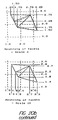
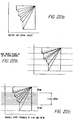
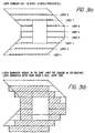
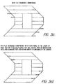
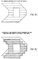
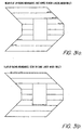
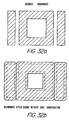
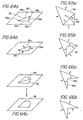
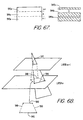
- This problem of holes was approached by deciding to create skin fill in the offset region between layers when the triangles forming that portion of a layer had a slope less than a specified amount from the horizontal plane.
- This skin fill is known as near-horizontal or near-flat skin.
- This technique worked well for completing the creation of solid parts.
- a version of this technique also completed the work necessary for solving the transition problem.
- the same version of this technique that solved the transition problem also yielded the best vertical feature accuracy of objects.
- EP-A-0 250 121 discloses an object where desired configuration includes a hollow interior portion.
- the present invention provides a stereolithography system for generating a three-dimensional object by forming successive, adjacent, cross-sectional laminae of that object at the face of a fluid medium capable of altering its physical state in response to appropriate synergistic stimulation, information defining the object being specially processed to reduce stress, curl and distortion, and increase resolution, strength, accuracy, speed and economy of reproduction, even for rather difficult object shapes, the successive laminae being automatically integrated as they are formed to define the desired three-dimensional object.
- Stereolithography harnesses the principles of computer generated graphics in combination with stereolithography, i.e., the application of lithographic techniques to the production of three-dimensional objects, to simultaneously execute computer aided design (CAD) and computer aided manufacturing (CAM) in producing three-dimensional objects directly from computer instructions.
- Stereolithography can be applied for the purposes of sculpturing models and prototypes in a design phase of product development, or as a manufacturing system, or even as a pure art form.
- Stepolithography is a method and apparatus for making solid objects by successively “printing” thin layers of a curable material, e.g., a UV curable material, one on top of the other.
- a curable material e.g., a UV curable material
- a programmed movable spot beam of UV light shining on a surface or layer of UV curable liquid is used to form a solid cross-section of the object at the surface of the liquid.
- the object is then moved, in a programmed manner, away from the liquid surface by the thickness of one layer, and the next cross-section is then formed and adhered to the immediately preceding layer defining the object. This process is continued until the entire object is formed.
- a body of a fluid medium capable of solidification in response to prescribed stimulation is first appropriately contained in any suitable vessel to define a designated working surface of the fluid medium at which successive cross-sectional laminae can be generated.
- an appropriate form of synergistic stimulation such as a spot of UV light or the like, is applied as a graphic pattern at the specified working surface of the fluid medium to form thin, solid, individual layers at the surface, each layer representing an adjacent cross-section of the three-dimensional object to be produced.
- information defining the object is specially processed to reduce curl and distortion, and increase resolution, strength, accuracy, speed and economy of reproduction.
- Superposition of successive adjacent layers on each other is automatically accomplished, as they are formed, to integrate the layers and define the desired three-dimensional object.
- a suitable platform to which the first lamina is secured is moved away from the working surface in a programmed manner by any appropriate actuator, typically all under the control of a micro-computer of the like. In this way, the solid material that was initially formed at the working surface is moved away from that surface and new liquid flows into the working surface position.
- this new liquid is, in turn, converted to solid material by the programmed UV light spot to define a new lamina, and this new lamina adhesively connects to the material adjacent to it, i.e., the immediately preceding lamina. This process continues until the entire three-dimensional object has been formed. The formed object is then removed from the container and the apparatus is ready to produce another object, either identical to the first object or an entirely new object generated by a computer or the like.
- the data base of a CAD system can take several forms.
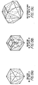
- One form consists of representing the surface of an object as a mesh of polygons, typically triangles. These triangles completely form the inner and outer surfaces of the object.
- This CAD representation also includes a unit length normal vector for each triangle. The normal points away from the solid which the triangle is bounding and indicate slope.
- This invention provides a means of processing CAD data, which may be provided as "PHIGS" or the like, into layer-by-layer vector data that can be used for forming models through stereolithography. Such information may ultimately be converted to raster scan output data or the like, without in any way departing from the spirit and scope of the invention.
- stereolithography is a three-dimensional printing process which uses a moving laser beam to build parts by solidifying successive layers of liquid plastic. This method enables a designer to create a design on a CAD system and build an accurate plastic model in a few hours.
- a stereolithographic process in accordance with the invention may include the following steps.
- the solid model is designed in the normal way on the CAD system, without specific reference to the stereolithographic process.
- Model preparation for stereolithography involves selecting the optimum orientation, adding supports, and selecting the operating parameters of the stereolithography system.
- the optimum orientation will (1) enable the object to drain, (2) have the least number of unsupported surfaces, (3) optimize important surfaces, and (4) enable the object to fit in the resin vat. Supports must be added to secure unattached sections and for other purposes, and a CAD library of supports can be prepared for this purpose.
- the stereolithography operating parameters include selection of the model scale and layer (slice) thickness.
- the surface of the solid model is then divided into triangles, typically "PHIGS".
- a triangle is the least complex polygon for vector calculations. The more triangles formed, the better the surface resolution and hence, the more accurate the formed object with respect to the CAD design.
- Data points representing the triangle coordinates and normals thereto are then transmitted typically as PHIGS, to the stereolithographic system via appropriate network communication such as ETHERNET.
- the software of the stereolithographic system then slices the triangular sections horizontally (X-Y plane) at the selected layer thickness.
- the stereolithographic unit next calculates the section boundary, hatch, and horizontal surface (skin) vectors.
- Hatch vectors consist of cross-hatching between the boundary vectors. Several "styles" or slicing formats are available. Skin vectors, which are traced at high speed and with a large overlap, form the outside horizontal surfaces of the object. Interior horizontal areas, those within top and bottom skins, are not filled in other than by cross-hatch vectors.
- the SLA then forms the object one horizontal layer at a time by moving the ultraviolet beam of a helium-cadmium laser or the like across the surface of a photocurable resin and solidifying the liquid where it strikes. Absorption in the resin prevents the laser light from penetrating deeply and allows a thin layer to be formed.
- Each layer is comprised of vectors which are typically drawn in the following order: border, hatch, and surface.
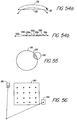
- the first layer that is drawn by the SLA adheres to a horizontal platform located just below the liquid surface.
- This platform is attached to an elevator which then lowers the elevator under computer control.
- the platform dips a short distance, such as several millimeters into the liquid to coat the previous cured layer with fresh liquid, then rises up a smaller distance leaving a thin film of liquid from which the second layer will be formed.
- the next layer is drawn. Since the resin has adhesive properties, the second layer becomes firmly attached to the first. This process is repeated until all the layers have been drawn and the entire three-dimensional object is formed. Normally, the bottom 0.25 inch (about 6.35mm) or so of the object is a support structure on which the desired part is built. Resin that has not been exposed to light remains in the vat to be used for the next part. There is very little waste of material.
- Post processing typically involves draining the formed object to remove excess resin, ultraviolet or heat curing to complete polymerization, and removing supports. Additional processing, including sanding and assembly into working models, may also be performed.
- Stereolithography has many advantages over currently used apparatus for producing plastic objects.
- the methods and apparatus of the present invention avoid the need of producing design layouts and drawings, and of producing tooling drawings and tooling.
- the designer can work directly with the computer and a stereolithographic device, and when he is satisfied with the design as displayed on the output screen of the computer, he can fabricate a part for direct examination. If the design has to be modified, it can be easily done through the computer, and then another part can be made to verify that the change was correct. If the design calls for several parts with interacting design parameters, the method of the invention becomes even more useful because of all of the part designs can be quickly changed and made again so that the total assembly can be made and examined, repeatedly if necessary.
- the data manipulation techniques of the present invention enable production of objects with reduced stress, curl and distortion, and increased resolution, strength, accuracy, speed and economy of production, even for difficult and complex object shapes.
- stereolithography is particularly useful for short run production because the need for tooling is eliminated and production set-up time is minimal. Likewise, design changes and custom parts are easily provided using the technique. Because of the ease of making parts, stereolithography can allow plastic parts to be used in many places where metal or other material parts are now used. Moreover, it allows plastic models of objects to be quickly and economically provided, prior to the decision to make more expensive metal or other material parts.
- a CAD generator 2 and appropriate interface 3 provide a data description of the object to be formed, typically in PHIGS format, via network communication such as ETHERNET or the like to an interface computer 4 where the object data is manipulated to optimize the data and provide output vectors which reduce stress, curl and distortion, and increase resolution, strength, accuracy, speed and economy of reproduction, even for rather difficult and complex object shapes.
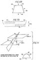
- the interface computer 4 generates layer data by slicing the CAD data, varying layer thickness, rounding polygon vertices, filling, generating flat skins, near-flat skins, up-facing and down-facing skins, scaling, cross-hatching, offsetting vectors and ordering vectors.
- the vector data and parameters from the computer 4 are directed to a controller subsystem 5 for operating the system stereolithography laser, mirrors, elevator and the like.
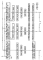
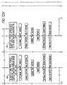
- FIGS. 2 and 3 are flow charts illustrating the basic system of the present invention for generating three-dimensional objects by means of stereolithography.
- UV curable chemicals are known which can be induced to change to solid state polymer plastic by irradiation with ultraviolet light (UV) or other forms of synergistic stimulation such as electron beams, visible or invisible light, reactive chemicals applied by ink jet or via a suitable mask.
- UV curable chemicals are currently used as ink for high speed printing, in processes of coating or paper and other materials, as adhesives, and in other specialty areas.
- Lithography is the art of reproducing graphic objects, using various techniques. Modern examples include photographic reproduction, xerography, and microlithography, as is used in the production of microelectronics. Computer generated graphics displayed on a plotter or a cathode ray tube are also forms of lithography, where the image is a picture of a computer coded object.
- Computer aided design (CAD) and computer aided manufacturing (CAM) are techniques that apply the abilities of computers to the processes of designing and manufacturing.
- a typical example of CAD is in the area of electronic printed circuit design, where a computer and plotter draw the design of a printed circuit board, given the design parameters as computer data input.
- a typical example of CAM is a numerically controlled milling machine, where a computer and a milling machine produce metal parts, given the proper programming instructions. Both CAD and CAM are important and are rapidly growing technologies.
- Stereolithography hamesses the principles of computer generated graphics, combined with UV curable plastic and the like, to simultaneously execute CAD and CAM, and to produce three-dimensional objects directly from computer instructions.
- Stereolittiography can be used to sculpture models and prototypes in a design phase of product development, or as a manufacturing device, or even as an art form.
- the present invention enhances the developments in stereolithography set forth in U.S. Patent No. 4,575,330, issued March 11, 1986, to Charles W. Hull, one of the inventors herein.
- Step 8 calls for generation of CAD or other data, typically in digital form, representing a three-dimensional object to be formed by the system.
- This CAD data usually defines surfaces in polygon format, triangles and normals perpendicular to the planes of those triangles, e.g., for slope indications, being presently preferred, and in a presently preferred embodiment of the invention conforms to the Programmer's Hierarchial Interactive Graphics System (PHIGS) now adapted as an ANSI standard.
- PHIGS Hierarchial Interactive Graphics System
- Step 9 the PHIGS data or its equivalent is converted, in accordance with the invention, by a unique conversion system to a modified data base for driving the stereolithography output system in forming three-dimensional objects.
- information defining the object is specially processed to reduce stress, curl and distortion, and increase resolution, strength and accuracy of reproduction.
- Step 10 in Figure 2 calls for the generation of individual solid laminae representing cross-sections of a three-dimensional object to be formed.
- Step 11 combines the successively formed adjacent laminae to form the desired three-dimensional object which has been programmed into the system for selective curing.
- stereolithography generates three-dimensional objects by creating a cross-sectional pattern of the object to be formed at a selected surface of a fluid medium, e.g., a UV curable liquid or the like, capable of altering its physical state in response to appropriate synergistic stimulation such as impinging radiation, electron beam or other particle bombardment, or applied chemicals (as by ink jet or spraying over a mask adjacent the fluid surface), successive adjacent laminae, representing corresponding successive adjacent cross-sections of the object, being automatically formed and integrated together to provide a step-wise laminar or thin layer buildup of the object, whereby a three-dimensional object is formed and drawn from a substantially planar or sheet-like surface of the fluid medium during the forming process.
- a fluid medium e.g., a UV curable liquid or the like
- Step 8 calls for generation of CAD or other data, typically in digital form, representing a three-dimensional object to be formed by the system.
- the PHIGS data is converted by a unique conversion system to a modified data base for driving the stereolithography output system in forming three-dimensional objects.
- Step 12 calls for containing a fluid medium capable of solidification in response to prescribed reactive stimulation.
- Step 13 calls for application of that stimulation as a graphic pattern, in response to data output from the computer 4 in Fig. 1, at a designated fluid surface to form thin, solid, individual layers at that surface, each layer representing an adjacent cross-section of a three-dimensional object to be produced.
- each lamina will be a thin lamina, but thick enough to be adequately cohesive in forming the cross-section and adhering to the adjacent laminae defining other cross-sections of the object being formed.
- Step 14 in Figure 3 calls for superimposing successive adjacent layers or laminae on each other as they are formed, to integrate the various layers and define the desired three-dimensional object.
- the fluid medium cures and solid material forms to define one lamina
- that lamina is moved away from the working surface of the fluid medium and the next lamina is formed in the new liquid which replaces the previously formed lamina, so that each successive lamina is superimposed and integral with (by virtue of the natural adhesive properties of the cured fluid medium) all of the other cross-sectional laminae.
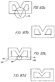
- the present invention also deals with the problems posed in transitioning between vertical and horizontal features.
- FIGS. 4-5 of the drawings illustrate various apparatus suitable for implementing the stereolithographic methods illustrated and described by the systems and flow charts of FIGS. 1-3.
- Stepolithography is a method and apparatus for making solid objects by successively “printing” thin layers of a curable material, e.g., a UV curable material, one on top of the other.
- a curable material e.g., a UV curable material
- a programmable movable spot beam of UV light shining on a surface or layer of UV curable liquid is used to form a solid cross-section of the object at the surface of the liquid.
- the object is then moved, in a programmed manner, away from the liquid surface by the thickness of one layer and the next cross-section is then formed and adhered to the immediately preceding layer defining the object. This process is continued until the entire object is formed.
- the data base of a CAD system can take several forms.
- One form as previously indicated, consists of representing the surface of an object as a mesh of triangles (PHIGS). These triangles completely form the inner and outer surfaces of the object.
- This CAD representation also includes a unit length normal vector for each triangle. The normal points away from the solid which the triangle is bounding.
- This invention provides a means of processing such CAD data into the layer-by-layer vector data that is necessary for forming objects through stereolithography.
- Stereolithography provides a general means of insuring adhesion between layers when making transitions from vertical to horizontal or horizontal to vertical sections, as well as providing a way to completely bound a surface, and ways to reduce or eliminate stress and strain in formed parts.
- a container 21 is filled with a UV curable liquid 22 or the like, to provide a designated working surface 23.
- a programmable source of ultraviolet light 26 or the like produces a spot of ultraviolet light 27 in the plane of surface 23.
- the spot 27 is movable across the surface 23 by the motion of mirrors or other optical or mechanical elements (not shown in FIG. 4) used with the light source 26.
- the position of the spot 27 on surface 23 is controlled by a computer control system 28.
- the system 28 may be under control of CAD data produced by a generator 20 in a CAD design system or the like and directed in PHIGS format or its equivalent to a computerized conversion system 25 where information defining the object is specially processed to reduce stress, curl and distortion, and increase resolution, strength and accuracy of reproduction.
- a movable elevator platform 29 inside container 21 can be moved up and down selectively, the position of the platform being controlled by the system 28. As the device operates, it produces a three-dimensional object 30 by step-wise buildup of integrated laminae such as 30a, 30b, 30c.
- the surface of the UV curable liquid 22 is maintained at a constant level in the container 21, and the spot of UV light 27, or other suitable form of reactive stimulation, of sufficient intensity to cure the liquid and convert it to a solid material is moved across the working surface 23 in a programmed manner.
- the elevator platform 29 that was initially just below surface 23 is moved down from the surface in a programmed manner by any suitable actuator. In this way, the solid material that was initially formed is taken below surface 23 and new liquid 22 flows across the surface 23. A portion of this new liquid is, in turn, converted to solid material by the programmed UV light spot 27, and the new material adhesively connects to the material below it. This process is continued until the entire three-dimensional object 30 is formed.
- the object 30 is then removed from the container 21, and the apparatus is ready to produce another object. Another object can then be produced, or some new object can be made by changing the program in the computer 28.
- the curable liquid 22, e.g., UV curable liquid, must have several important properties: (A) It must cure fast enough with the available UV light source to allow practical object formation times. (B) It must be adhesive, so that successive layers will adhere to each other. (C) Its viscosity must be low enough so that fresh liquid material will quickly flow across the surface when the elevator moves the object. (D) It should absorb UV so that the film formed will be reasonably thin. (E) It must be reasonably insoluble in that same solvent in the solid state, so that the object can be washed free of the UV cure liquid and partially cured liquid after the object has been formed. (F) It should be as non-toxic and nonirritating as possible.
- the cured material must also have desirable properties once it is in the solid state. These properties depend on the application involved, as in the conventional use of other plastic materials. Such parameters as color, texture, strength, electrical properties, flammability, and flexibility are among the properties to be considered. In addition, the cost of the material will be important in many cases.
- the UV curable material used in the presently preferred embodiment of a working stereolithograph is DeSoto SLR 800 stereolithography resin, made by DeSoto, Inc. of Des Plains, Illinois.
- the light source 26 produces the spot 27 of UV light small enough to allow the desired object detail to be formed, and intense enough to cure the UV curable liquid being used quickly enough to be practical.
- the source 26 is arranged so it can be programmed to be turned off and on, and to move, such that the focused spot 27 moves across the surface 23 of the liquid 22.
- the spot 27 moves, it cures the liquid 22 into a solid, and "draws" a solid pattern on the surface in much the same way a chart recorder or plotter uses a pen to draw a pattern on paper.
- the light source 26 is typically a helium-cadmium ultraviolet laser such as the Model 4240-N HeCd Multimode Laser, made by Liconix of Sunnyvale, California.
- means may be provided to keep the surface 23 at a constant level and to replenish this material after an object has been removed, so that the focus spot 27 will remain sharply in focus on a fixed focus plane, thus insuring maximum resolution in forming a high layer along the working surface.
- the elevator platform 29 is used to support and hold the object 30 being formed, and to move it up and down as required. Typically, after a layer is formed, the object 30 is moved beyond the level of the next layer to allow the liquid 22 to flow into the momentary void at surface 23 left where the solid was formed, and then it is moved back to the correct level for the next layer.
- the requirements for the elevator platform 29 are that it can be moved in a programmed fashion at appropriate speeds, with adequate precision, and that it is powerful enough to handle the weight of the object 30 being formed. In addition, a manual fine adjustment of the elevator platform position is useful during the set-up phase and when the object is being removed.
- the elevator platform 29 can be mechanical, pneumatic, hydraulic, or electrical and may also be optical or electronic feedback to precisely control its position.
- the elevator platform 29 is typically fabricated of either glass or aluminum, but any material to which the cured plastic material will adhere is suitable.
- a computer controlled pump may be used to maintain a constant level of the liquid 22 at the working surface 23.
- Appropriate level detection system and feedback networks can be used to drive a fluid pump or a liquid displacement device, such as a solid rod (not shown) which is moved out of the fluid medium as the elevator platform is moved further into the fluid medium, to offset changes in fluid volume and maintain constant fluid level at the surface 23.
- the source 26 can be moved relative to the sensed level 23 and automatically maintain sharp focus at the working surface 23. All of these alternatives can be readily achieved by appropriate data operating in conjunction with the computer control system 28.
- SLICE portion of the processing referred to as "SLICE” takes in the object that is to be built, together with any scaffolding or supports that are necessary to make it more buildable. These supports are typically generated by the user's CAD. The first thing SLICE does is to find the outlines of the object and its supports.
- SLICE defines each microsection or layer one at a time under certain specified controlling styles. SLICE produces a boundary to the solid portion of the object. If, for instance, the object is hollow, there will be an outside surface and an inside one. This outline then is the primary information. The SLICE program then takes that outline or series of outlines and, considering that the building of an outside skin and an inside skin won't join to one another, since there will be liquid between them and it will collapse, SLICE turns this into a real product, a real part by putting in cross-hatching between the surfaces, or solidifying everything in between or adding skins where it's so gentle a slope that one layer wouldn't join on top of the next, remembering past history or slope of the triangles (PHIGS).
- SLICE does all those things and other programs then use some lookup tables of the chemical characteristics of the photopolymer, how powerful the laser is, and related parameters to indicate how long to expose each of the output vectors used to operate the system.
- Those output vectors can be divided into identifiable groups. One group consists of the boundaries or outlines. Another group consists of cross-hatches.
- a third group consists of skins and there are subgroups of those, such as upward facing skins, and downward facing skins which have to be treated slightly differently. These subgroups are all tracked differently because they may get slightly different treatment; in the process, the output data is then appropriately managed to form the desired object and supports.
- the elevator platform 29 is raised and the object is removed from the platform for post processing.
- each container 21 there may be several containers 21 used in the practice of the invention, each container having a different type of curable material that can be automatically selected by the stereolithographic system.
- the various materials might provide plastics of different colors, or have both insulating and conducting material available for the various layers of electronic products.
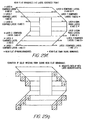
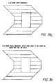
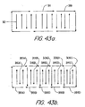
- FIG. 5 of the drawings there is shown an alternate configuration of a stereolithograph wherein the UV curable liquid 22 or the like floats on a heavier UV transparent liquid 32 which is non-miscible and non-wetting with the curable liquid 22.
- ethylene glycol or heavy water are suitable for the intermediate liquid layer 32.
- the three-dimensional object 30 is pulled up from the liquid 22, rather than down and further into the liquid medium, as shown in the system of Figure 3.
- the UV light source 26 in Figure 5 focuses the spot 27 at the interface between the liquid 22 and the non-miscible intermediate liquid layer 32, the UV radiation passing through a suitable UV transparent window 33, of quartz or the like, supported at the bottom of the container 21.
- the curable liquid 22 is provided in a very thin layer over the non-miscible layer 32 and thereby has the advantage of limiting layer thickness directly rather than relying solely upon absorption and the like to limit the depth of curing since ideally an ultrathin lamina is to be provided. Hence, the region of formation will be more sharply defined and some surfaces will be formed smoother with the system of Figure 5 than with that of Figure 4. In addition a smaller volume of UV curable liquid 22 is required, and the substitution of one curable material for another is easier.
- a commercial stereolithography system will have additional components and subsystems besides those previously shown in connection with the schematically depicted systems of FIGS. 1-5.
- the commercial system would also have a frame and housing, and a control panel. It should have means to shield the operator from excess UV and visible light, and it may also have means to allow viewing of the object 30 while it is being formed.
- Commercial units will provide safety means for controlling ozone and noxious fumes, as well as conventional high voltage safety protection and interlocks. Such commercial units will also have means to effectively shield the sensitive electronics from electronic noise sources.
- an electron source, a visible light source, or an x-ray source or other radiation source could be substituted for the UV light source 26, along with appropriate fluid media which are cured in response to these particular forms of reactive stimulation.
- an electron source, a visible light source, or an x-ray source or other radiation source could be substituted for the UV light source 26, along with appropriate fluid media which are cured in response to these particular forms of reactive stimulation.
- alphaoctadecylacrylic acid that has been slightly prepolymerized with UV light can be polymerized with an electron beam.
- poly(2,3-dichloro-1-propyl acrylate) can be polymerized with an x-ray beam.
- the commercialized SLA is a self-contained system that interfaces directly with the user's CAD system.
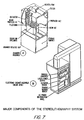
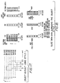
- the SLA as shown in FIGS. 6 and 7, consists of four major component groups: the slice computer terminal, the electronic cabinet assembly, the optics assembly, and the chamber assembly.
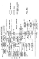
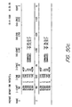
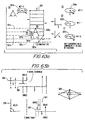
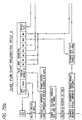
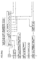
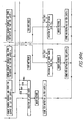
- a block diagram of the SLA is shown in Figure 8.
- the electronic cabinet assembly includes the process computer (disc drive), keyboard, monitor, power supplies, ac power distribution panel and control panel.
- the computer assembly includes plug-in circuit boards for control of the terminal, high-speed scanner mirrors, and vertical (Z-stage) elevator. Power supplies for the laser, dynamic mirrors, and elevator motor are mounted in the lower portion of the cabinet.
- the control panel includes a power on switch/indicator, a chamber light switch/indicator, a laser on indicator, and a shutter open indicator.
- Operation and maintenance parameters including fault diagnostics and laser performance information, are also typically displayed on the monitor. Operation is controlled by keyboard entries. Work surfaces around the key-board and disc drive are covered with formica or the like for easy cleaning and long wear.
- the helium cadmium (HeCd) laser and optical components are mounted on top of the electronic cabinet and chamber assembly.
- the laser and optics plate may be accessed for service by removing separate covers.
- a special tool is required to unlock the cover fasteners and interlock switches are activated when the covers are removed.
- the interlocks activate a solenoid-controlled shutter to block the laser beam when either cover is removed.
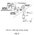
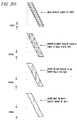
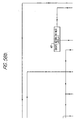
- the shutter assembly As shown in Figure 9, the shutter assembly, two ninety degree beam-turning mirrors, a beam expander, an X-Y scanning mirror assembly, and precision optical window are mounted on the optics plate.
- the rotary solenoid-actuated shutters are installed at the laser output and rotate to block the beam when a safety interlock is opened.
- the ninety degree beam-turning mirrors reflect the laser beam to the next optical component.
- the beam expander enlarges and focuses the laser beam on the liquid surface.
- the high speed scanning mirrors direct the laser beam to trace vectors on the resin surface.
- a quartz window between the optics enclosure and reaction chamber allows the laser beam to pass into the reaction chamber, but otherwise isolates the two regions.
- the chamber assembly contains an environmentally-controlled chamber, which houses a platform, reaction vat, elevator, and beam profiler.
- the chamber in which the object is formed is designed for operator safety and to ensure uniform operating conditions.
- the chamber may be heated to approximately 40° C (104° F) and the air is circulated and filtered.
- An overhead light illuminates the reaction vat and work surfaces.
- An interlock on the glass access door activates a shutter to block the laser beam when opened.
- the reaction vat is designed to minimize handling of the resin. It is typically installed in the chamber on guides which align it with the elevator and platform.
- the object is formed on a platform attached to the vertical axis elevator, or Z-stage.
- the platform is immersed in the resin vat and it is adjusted incrementally downward while the object is being formed. To remove the formed part, it is raised to a position above the vat. The platform is then disconnected from the elevator and removed from the chamber for post processing. Handling trays are usually provided to catch dripping resin.
- the beam profilers are mounted at the sides of the reaction vat at the focal length of the laser.
- the scanning mirror is periodically commanded to direct the laser beam onto the beam profiler, which measures the beam intensity profile.
- the data may be displayed on the terminal, either as a profile with intensity contour lines or as a single number representing the overall (integrated) beam intensity. This information is used to determine whether the mirrors should be cleaned and aligned, whether the laser should be serviced, and what parameter values will yield vectors of the desired thickness and width.
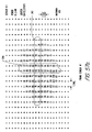
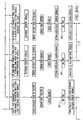
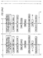
- FIG. 10 A software diagram of the SLA is shown in Figure 10.
- a CAD system can be used to design a part in three-dimensional space. This is identified as the object file.
- supports In order to generate the part, supports must be added to prevent distortion..This is accomplished by adding the necessary supports to the CAD part design and creating a CAD support file. The resultant two or more CAD generated files are then physically inserted into the slice computer through ETHERNET.
- the stereolithography apparatus builds the part one layer at a time starting with the bottom layer.
- the SLICE computer breaks down the CAD part into individual horizontal slices.
- the SLICE computer also calculates where hatch vectors will be created. This is done to achieve maximum strength as each layer is constructed.
- the SLICE computer may be a separate computer with its own keyboard and monitor. However, the SLICE computer may share a common keyboard and monitor with the PROCESS computer.
- the operator can vary the thickness of each slice and change other parameters of each slice with a User Interface program.
- the SLICE computer may use the XENIX or UNIX operating system and is connected to the SLA PROCESS computer by an ETHERNET network data bus or the like.
- the sliced files are then transferred to the PROCESS computer through ETHERNET.
- the PROCESS computer merges the sliced object and support files into a layer control file and a vector file.
- the operator then inserts the necessary controls needed to drive the stereolithography apparatus in the layer control and a default parameter file.
- the vector file is not usually edited.
- the operator can strengthen a particular volume of the part by inserting rivets. This is accomplished by inserting the necessary parameters to a critical volume file prior to merging of the sliced files.
- the MERGE program integrates the object, support, and critical volume files and inserts the resultant data in the layer control file.
- the operator can edit the layer control file and change the default parameter file.
- the default parameter file contains the controls needed to operate the stereolithography apparatus to build the part.
- the PROCESS computer uses the MSDOS operating system and is directly connected to the stereolithography apparatus.
- Stereolithography is a three-dimensional printing process which uses a moving laser beam to build parts by solidifying successive layers of liquid plastic. This method enables a designer to create a design on a CAD system and build an accurate plastic model in a few hours.
- the stereolithographic process may comprise of the following steps.
- the solid model is designed in the normal way on the CAD system, without specific reference to the stereolithographic process.
- Model preparation for stereolithography involves selecting the optimum orientation, adding supports, and selecting the operating parameters of the stereolithography system.
- the optimum orientation will (1) enable the object to drain, (2) have the least number of unsupported surfaces, (3) optimize important surfaces, and (4) enable the object to fit in the resin vat. Supports must be added to secure unattached sections and for other purposes; a CAD library of supports can be prepared for this purpose.
- the stereolithography operating parameters include selection of the model scale and layer (slice) thickness.
- the surface of the solid model is then divided into triangles, typically "PHIGS".
- a triangle is the least complex polygon for vector calculations. The more triangles formed, the better the surface resolution and hence the more accurate the formed object with respect to the CAD design
- Data points representing the triangle coordinates are then transmitted to the stereolithographic system via appropriate network communications.
- the software of the stereolithographic system then slices the triangular sections horizontally (X-Y plane) at the selected layer thickness.
- the stereolithographic unit next calculates the section boundary, hatch, and horizontal surface (skin) vectors.
- Hatch vectors consist of cross-hatching between the boundary vectors.
- Skin vectors which are traced at high speed and with a large overlap, form the outside horizontal surfaces of the object.
- Interior horizontal areas, those within top and bottom skins, are not filled in other than by cross-hatch vectors.
- the SLA then forms the object one horizontal layer at a time by moving the ultraviolet beam of a helium-cadmium laser across the surface of a photocurable resin and solidifying the liquid where it strikes. Absorption in the resin prevents the laser light from penetrating deeply and allows a thin layer to be formed.
- Each layer is comprised of vectors which are drawn in he following order: border, hatch, and surface.
- the first layer that is drawn by the SLA adheres to a horizontal platform located just below the liquid surface.
- This platform is attached to an elevator which then lowers its vertically under computer control.
- the platform dips several millimeters into the liquid to coat the previous cured layer with fresh liquid, then rises up a smaller distance leaving a thin film of liquid from which the second layer will be formed.
- the next layer is drawn. Since the resin has adhesive properties, the second layer becomes firmly attached to the first. This process is repeated until all the layers have been drawn and the entire three-dimensional object is formed. Normally, the bottom 0.25 inch or so of the object is a support structure on which the desired part is built. Resin that has not been exposed to light remains in the vat to be used for the next part. There is very little waste of material.
- Post processing involves draining the formed object to remove excess resin, ultraviolet or heat curing to complete polymerization, and removing supports. Additional processing, including sanding and assembly into working models, may also be performed.
- the stereolithographic method and apparatus has many advantages over currently used methods for producing plastic objects.
- the method avoids the need of producing design layouts and drawings, and of producing tooling drawings and tooling.
- the designer can work directly with the computer and a stereolithographic device, and when he is satisfied with the design as displayed on the output screen of the computer, he can fabricate a part for direct examination. If the design has to be modified, it can be easily done through the computer, and then another part can be made to verify that the change was correct. If the design calls for several parts with interacting design parameters, the method becomes even more useful because all of the part designs can be quickly changed and made again so that the total assembly can be made and examined, repeatedly if necessary.
- part production can begin immediately, so that the weeks and months between design and production are avoided. Ultimate production rates and parts costs should be similar to current injection molding costs for short run production, with even lower labor costs than those associated with injection molding. Injection molding is economical only when large numbers of identical parts are required. Stereolithography is useful for short run production because the need for tooling is eliminated and production set-up time is minimal. Likewise, design changes and custom parts are easily provided using the technique. Because of the ease of making parts, stereolithography can allow plastic parts to be used in many places where metal or other material parts are now used. Moreover, it allows plastic models of objects to be quickly and economically provided, prior to the decision to make more expensive metal or other material parts.
- Stereolithography embodies the concept of taking three-dimensional computer data describing an object and creating a three-dimensional plastic replica of the object. Construction of an object is based on converting the three-dimensional computer data into two-dimensional data representing horizontal layers and building the object layer by layer.
- the software that takes us from the three-dimensional data defining the object to vector data is called "SLICE".
- FIGS. 13 and 14 illustrate a sample CAD designed object. Figure 15 shows typical slicing of CAD object.
- FIGS. 16, 17 and 18 show slice (layer) data forming the object.
- CAD data files are referred to as STL files. These STL files divide the surface area of an object into triangular facets. The simpler the object the fewer the triangles needed to describe it, and the more complex the object or the more accuracy used to represent its curvatures the more triangles required to describe it. These triangles encompass both inner and outer surfaces.
- Figure 33 is a software architecture flowchart depicting in greater detail the overall data flow, data manipulation and data management in a stereolithography system incorporating the features of the invention
- triangles are represented by four sets of three numbers each.
- Each of the first three sets of numbers represents a vertex of the triangle in three-dimensional space.
- the fourth set represents the coordinates of the normal vector perpendicular to the plane of the triangle.
- This normal is considered to start at the origin and point to the coordinates specified in the STL file.
- this normal vector is also of unit length (i.e., one CAD unit).
- the normal vector can point in either of two directions, but by convention, the direction we have chosen points from solid to hollow (away from the solid interior of the object that the triangle is bounding).
- attribute designation is also associated with each triangle.
- Figure 19a shows a faceted sketch of a solid cube.
- Figure 19b shows a faceted sketch of a hollow cube.
- Figure 19c shows a faceted sketch of a solid octagon shaped cylinder.
- Scaling of an STL file involves a consideration of SLICE, the slicing program that converts the three-dimensional data into two-dimensional vectors, which is based on processing integers.
- the CAD units in which an object is dimensioned, and therefore the STL file, are arbitrary.
- a scale factor is used to divide the CAD units into bits (1 bit is approximately .3 mil), so that slicing can be done based on bits instead of on the units of design. This provides the ability to maximize the resolution with which an object will be built regardless of what the original design units were.
- Figure 20a shows a faceted CAD designed object in gridded space (two-dimensional).
- Figure 20b shows a faceted CAD designed object after rounding of triangles - Scale 1 - Scale 4 - Scale 10.
- Figure 20c shows a faceted CAD designed object after rounding of triangles in which triangle overlap occurs.
- Rounding of triangle vertices provides several advantages over allowing them to remain at the locations that they were originally at in the STL file. If vertices are rounded then all horizontal triangles are moved to slicing layers. Thus, when flat skin is created .(derived from horizontal triangles) the skin will have excellent fit within the boundaries at a particular layer. In addition, the cross-hatching between the walls of objects will have more accurate placement. Cross hatching is based on hatch paths intersecting boundaries and then determining whether to turn hatching on and off. If a hatch path should strike a vertex point it would be difficult to make an accurate decision whether to turn hatch on or off. By rounding vertices, SLICE knows exactly where they are (in the vertical dimension) and can therefore avoid them when creating boundaries (which are used in the process of generating hatch).
- Rounding of vertices to slicing layers is more likely to cause overlap of triangles than is rounding to the nearest scale bit.
- certain slicing styles require creating vectors 1 bit off the slicing layers so that the part comes out with the best vertical dimension. These styles are discussed in more detail farther on in this application.
- the problems associated with rounding of vertices to slicing layers cannot be solved by using arbitrarily small slicing layers or by limiting the minimum size of triangles.
- One possible way of minimizing the problem is to put a limit on the maximum dimension of triangles to slightly over one layer thickness. This could be used to reduce the number of overlapping surfaces.
- the proposed hatching algorithm will enable the handling of regions of overlapping triangles in a consistent and reliable manner.
- Figure 21a illustrates a faceted CAD designed object after rounding of triangles based on scale factor.
- Figure 21b shows a faceted CAD designed object after rounding of triangles in the vertical to slicing layers - layer thickness 20 mils.
- Figure 21c shows a faceted CAD designed object after rounding of triangles in the vertical to slicing layers - layer thickness 5 mils.
- the vertical distance between layers can be varied depending on the vertical resolution needed in different areas.
- the selection of layer thickness is based on three distinct considerations: 1) desired resolution, 2) structural strength required of the layer, and 3) time allowed for building the object. Each of these factors is affected by layer thickness.
- Item 1 resolution, is the most obvious item that is affected. The resolution of vertical features is inversely proportional to layer thickness.
- Item 2 structural strength, is proportional to cure thickness, and cure thickness is generally based on layer thickness plus a constant or a percentage of layer thickness.
- Another way of minimizing this problem is to design parts as separate objects that can be sliced separately using different layer thicknesses. So item 2 is sometimes a problem with regard to decreasing layer thickness but not necessarily.
- Item 3 may or may not represent a problem when layer thickness is decreased.
- the time required to build a given part is based on three tasks: laser scanning time, liquid settling time, and number of layers per given thickness. As the layer thickness decreases, the liquid settling time increases, number of layers per unit thickness increases, and the drawing time decreases. On the other hand, with increasing layer thickness, the settling time decreases, number of layers per unit thickness decreases, and the drawing time increases.
- Figure 22a shows a faceted CAD designed object to be sliced.
- Figure 22b shows a faceted CAD designed object sliced at 20 mil layers.
- Figure 22c illustrates a faceted CAD designed object sliced at variable layer thickness of 5 mil and 20 mil.
- boundaries that can be used to form the edges of layers and features when building parts. These boundaries include the layer boundary, down facing flat skin boundary, up facing flat skin boundary, down facing near-flat skin boundary, and up facing near-flat skin boundary.
- Triangles are categorized into three main groups after they are rounded to both scale bits and to layers: scan triangles, near-flat triangles, and flat triangles.
- Flat triangles are those which have all three vertices all lying on the same layer.
- Near-flat triangles are those having normal vectors within some minimum angle from the vertical. All remaining triangles are scan triangles, i.e., those having normals outside the minimum angle from the vertical.
- Layer boundaries are created at the line of intersection of scan and near-flat triangles with a horizontal plane intersecting the object at a vertical level slightly offset from the slicing layer.
- Each scan and near-flat triangle that is present at this slight vertical offset from a given layer will be used to create one vector that will form part of the layer boundary.
- Each triangle will have two points that cross a given layer and one of these points will be used as a starting point for a vector and the other point will be used as the ending point of the vector. Since triangles form complete surfaces around the object to be formed, both inside and outside, there will be vectors formed that will make a complete boundary around the layer.
- Figure 23a shows a side view of the intersection of triangles with a layer, and vectors that are created at this intersection.
- Figure 23b shows a side view of a faceted section of an object, the slicing layer, the offset, and the vectors created including a point vector.
- boundary vectors should be created right at the intersection of the triangles with the slicing layer but this creates several problems that can be readily solved by creating the boundary vectors from the intersection of triangles with a horizontal plane that is just slightly above or below the slicing layer.
- This concept of creating boundary vectors which are slightly offset from the slicing layer introduces some minor problems but they an be made negligible by making the offset arbitrarily small.
- a preferred offset is one scale bit off the actual layer level. For discussion's sake, an offset one bit above the slicing layer will be considered by way of example (STYLE 1). The table below is illustrative.
- Part design units inches (1 inch 25.4 mm) Slice scale factor 1000 Layer spacing 20 Vertical location of part in CAD space 1.000 to 1.100 inches Location of layers in scaled units 1000, 1020, 1040, 1060, 1080, 1100 Locations of intersecting plane for determining boundary vectors in scaled units 1001, 1021, 1041, 1061, 1081, 1101 Layer designations associated with boundary vectors: 1000, 1020, 1040 1060, 1080
- the original object was 100 mils tall. If SLICE would have obtained boundary vectors right at the slicing layer, it would have had six layers (to be built at 20 mils each) forming a 120 mil object, but since it sliced 1 bit above the slicing layer, it ends up with only five layers (to be built at 20 mils each) forming a 100 mil object.
- the vertical offset for obtaining boundary vectors creates one potential problem: If the part has a near horizontal boundary at a particular layer then if SLICE obtains the boundary vectors from one bit above the layer, they may be considerably different from the vectors that would have been formed if the boundaries were obtained from the exact slicing level. This problem can be minimized by making the one bit offset extremely small compared to the part dimensions. This is why the one bit offset is preferred.
- the offset described above avoids several potential difficulties: The first is that the object's vertical dimensions would be otherwise distorted. These distortions can take several forms: the overall height of the part would be one layer too tall, the bottom of all vertical openings would be placed one layer too high relative to the bottom of the part, and all these openings would be one layer shorter than desired. All of these distortions can be summarized by stating that all up facing features will be one layer too high relative to all down facing features.
- the second problem deals with misplaced cross-hatch vectors (generated using one of SLICE's hatching algorithms). This is manifested in two ways: one is lack of consistency in generating cross-hatch for supporting up facing flat skin, the second way is the drawing of stray cross-hatch vectors running through hollow places within the object and/or cross-hatching missing from within the walls of the object.
- Figure 23c illustrates a side view of a CAD designed object with internal features (windows) after rounding has occurred.
- Figure 23d shows a side view of the same object after being built from obtaining boundary vectors at the slicing layer.
- Figure 23e is a side view of the same object after being built from obtaining boundary vectors at one bit above the slicing layer.
- the first algorithm is based on an on-off switching of cross-hatch as layer border vectors are encountered.
- the second algorithm is based on knowing where the solid portion of the object is and, therefore, where cross-hatching should be placed based on the direction that normal vectors point.
- the types of hatch are 1) hatch that runs parallel to the X-axis, 2) hatch that runs parallel to the Y-axis, and 3) hatch that runs at 60 degrees and 120 degrees to the X-axis.
- the spacing between the hatch vectors is based on the number of bits specified in a slice command line for the parameters -Hx, -Hy, -Ha,-MIA, which parameters are defined below:
- the methods of implementing the hatch vectors are 1) implement all generated hatch or 2) implement only those hatch vectors that intersect both boundaries at angles greater than that specified with the slice command - MIA.
- MIA option allows one to generate near-radial (nearly perpendicular to the boundaries) cross-hatch which can be an advantage in the case of objects that are prone to curl.
- Another feature added to the algorithm to minimize misplacement or non-placement of hatch vectors involves a determination of the slope (in the XY plane) of each of the boundary vectors that was used in the determination of an intersection point. If an intersection point is listed more than once, the slopes associated with it are used to determine how to interpret the point. If a point is derived from two vectors with the same sign (+ or -) of slope, the point is considered a boundary. If the slopes have the opposite sign the point is ignored.
- the second process is based on using the normal vectors which are supplied with each triangle in the STL file.
- each vector created is derived from a triangle that intersects a horizontal plane one bit above the slicing layer.
- Each boundary vector is stored as a beginning point (x,y) and an ending point (x,y) and associated with each vector are six attributes. These attributes describe the orientation of the normal vector that is associated with the triangle from which the vector was obtained. These six attributes are 1) did the normal point along the positive x axis? (true or false), 2) did the normal point along the -x axis?, 3) did the normal vector point along the +y axis?, 4) did the normal vector point along the -y axis?, 5) did the normal vector point along the +z axis?, 6) did the normal vector point along the -z axis.
- SLICE determines where to place hatch vectors
- SLICE still uses the intersection of a hatch path with boundary vectors to trigger a need to make a decision, but SLICE now bases whether or not to turn on or off the hatching based on whether the normals indicate SLICE is going into or out of solid. What actually happens is that SLICE determines the point at which each boundary vector intersects the hatching line, and puts this point in a list along with its normal information. This is done with each boundary vector for each hatch path. Each point is evaluated as to whether it indicates that hatch should be turned on or off or continued in the same state.
- the present utilization of this algorithm is based on original normals supplied by the STL file and not on normals recalculated after rounding of triangles to scale bits and slicing layers has occurred.
- the second algorithm can cause the misplacement or non-placement of hatch vectors if separate objects that overlap in space are combined in the same STL file. Since these situations represent physically impossible objects, the CAD designer should be able to avoid them when creating STL files. If, for design convenience, an overlapping of objects would be convenient, the objects should be placed into separate STL files and sliced separately.
- the present as well as the proposed algorithm can cause the misplacement of vectors if dimensions of features or hollows in CAD space cause them to collapse in some manner (due to chosen scale or layer thickness), thereby forming a double skin in some regions of an object. The formation of misplaced hatch vectors has a different source for these two algorithms.
- the present algorithm can misplace hatch the entire distance along the collapsed region except at the starting and ending points of boundary vectors. At these points, it will make the right decision some of the time. However, the alternative algorithm will make the proper decision at every point along the collapsed region except at the starting and ending points of boundary vectors. At these points, it will make the right decision a portion of the time. Therefore, it is not advisable to design parts that have regions where a collapse can occur, but if this is not possible, the alternative algorithm will at least reduce the likelihood of stray vectors (from the above mentioned source).
- the present algorithm can misplace hatch vectors when a hatch line intersects a boundary at a junction point where two or more boundary vectors meet. However, the improved algorithm will not misplace vectors in this situation.
- All three algorithms implement cross-hatch along the X-axis only.
- To derive hatch parallel to the Y-axis the part is rotated 90°, hatched along the new X-axis and then rotated back.
- To derive 60 and 120° hatch the object is rotated 60 and 120°, respectively, hatched along the new X-axis, then rotated back into place.
- Figure 24 is a top view of a cross-section of an object showing how hatch paths are determined.
- Figure 24a is a top view of an object filled by X hatch.
- Figure 24b is a top view of an object filled by Y hatch.
- Figure 24c is a top view of an object filled by 60/120 hatch.
- Figure 24d is a top view of a layer of an object completely filled in its solid regions.
- Figure 24e is a top view of a layer of an object properly filled in by cross-hatch (X & Y).
- Figure 24f is a top view of a layer of boundary vectors along with hatch vectors generated by the first algorithm (X & Y).
- Figure 24g is a top view of boundary vectors along with hatch vectors generated by the second algorithm (X & Y).
- Figure 24h is a top view of a layer of boundary vectors along with hatch vectors generated by the proposed algorithm (X & Y).
- FIGS. 24i and 24j are top views of cross-sections of an object hatched using various MIAs.
- FIGS. 24k is a schematic boundary diagram.
- Problems to be considered include: 1) how to specify in CAD or otherwise which triangles are regular and which are not, 2) how to insure triangles that form closed loops are of one type only, 3) how would tangent following be implemented (vector offsetting to account for line width a/k/a beam width compensation, discussed in more detail later), 4) would hatch associated with near-flat and flat boundaries still be used, etc.
- Flat skin is generated from completely horizontal triangles.
- a horizontal triangle is one which has all three vertices at the same layer. Rounding of triangle vertices may produce flat triangles from triangles that were not originally horizontal.
- the first step in forming flat skins is to separate them into two groups, one consisting of up-facing triangles (up-pointing normals) and the other consisting of down-facing triangles.
- the triangles in each group are then ordered according to the layers which they belong to.
- the edges of each triangle which belong to a particular layer are interpreted as boundary vectors for flat up or down-facing skin. These boundary vectors continue to tessellate an area of skin into a group of triangles.
- SLICE next removes all pairs of duplicate boundary vectors.
- the filling of the flat skin boundaries is based on the same algorithms as mentioned for cross-hatching above. Therefore, the intersection of a fill line with a boundary triggers the need for a decision to be made as to whether to turn on fill, turn off fill, or continue as is.
- the decision on what to do is again based on either an odd-even turn on/turn off condition or on the consideration of the direction of the normal vectors associated with each boundary segment (vector).
- vectors are created by SLICE, and are associated with the boundary vectors, unlike the normals discussed earlier, which are created by the CAD system and are associated with the triangles.
- the normal associated with each vector is derived from the triangle it was obtained from, whereas the normal associated with each flat triangle points only in the vertical direction and therefore cannot be used to determine any characteristics designating the inside or outside of the triangle.
- the technique used to determine the normals for a flat skin boundary is based on the analysis of the three vectors that make up the boundary of a triangle as a group. The technique is to compare the coordinates of the vertices making up a vector to those of the third point of the triangle to determine which way is outside the triangle (relative to the vector). This information, along with the slope of the boundary vector, is sufficient to determine the proper normal direction. This same procedure is done for each of the segments that form the boundaries of a triangle.
- the normal is then reduced to designate which quadrant it points in, and that information is saved with the boundary segment data (beginning and endpoints). This procedure is repeated for all flat triangles. Then all pairs of duplicate boundary vectors are removed for a given skin type on a given layer. The fill vectors can then be calculated using the same algorithm previously described for hatch vectors.
- a further improved technique of generating skins is based on the original direction of the vertical component of the triangle normals as supplied in the STL file. Problems may occur when flat triangles on the edge of a flat surface flip over after rounding to vertices. These problems might occur because the segment normals associated with skin boundary vectors (from flipped triangles) may end up pointing toward the area requiring skin instead of away from it. This, in turn, can cause the misplacement of hatch or fill vectors.
- the first solution is based on considerations similar to those used to develop the normal-sign summation hatching process.
- Six situations can develop when flat triangles flip over: 1) the flipped triangle forms a single flat surface, 2) the flipped triangle forms a single and a double flat surface, 3) the flipped triangle forms a double surface only, 4) the flipped triangle forms a double and a triple surface, 5) the flipped triangle forms a triple surface only, and 6) other situations that can develop between flat triangles involving features collapsing to single layers, yielding flat up and down-facing triangles covering the same area on a single layer. These situations are very similar to those used to develop the normal-sign summation hatching process.
- the summation technique used for layer hatching computes the net boundary at the intersection of boundaries with hatch paths
- the technique for skinning is based on determining net normals for areas based on addition of areas with like normals and subtraction of areas with opposite normals (up-facing, and down-facing). Then, the determination as to whether an area receives up-facing skin, down-facing skin, or no skin is based on whether the net normal of the areas points up, down, or does not exist.
- the directions of the normals must be determined after distortion of the triangles.
- FIG. 25h is a top view of flat triangles forming single/double surfaces before flipping, after flipping, with segment normals, after cancellation of duplicate pairs, after splitting of vectors, and after loop determination (two).
- FIGS. 26a and 26b are side views of boundaries on two consecutive layers and the associated variables for determination of the MSA.
- Figure 26c is a part requiring near-flat skin (the test box).
- SLICE can process these specific triangles to yield boundary vectors for this skin. It would be difficult to base the development of near-flat skin on differences between layer borders from one layer to the next. Also, to consistently determine the proper near-flat fill, this fill must be generated from the intersection of near-flat triangles right at the slicing layers, not one bit up or down. As with all fill and hatch vectors, SLICE must first determine the boundaries between which it wants to fill. Once these boundaries are determined, the fill will be based on the same algorithms on which layer hatch and flat skin fill are based.
- Figure 26d is a near-flat triangle intersecting two layers and forming two boundary vectors.
- the remaining two sides of the trapezoid are formed by producing straight non-intersecting lines from the endpoints of the first segment to the endpoints of the second segment.
- SLICE has formed a two-dimensional boundary (in a plane) from a particular near-flat triangle, that can be filled with skin and/or hatch.
- the next step is to determine the segment normal vectors associated with each of these boundary vectors to clarify what is inside and what is outside of the trapezoid. This determination is very similar to that which was done for flat skin boundaries.
- Figure 27a is a top view of a possible order to drawing boundary vectors when they are not ordered.
- Figure 27b is a top view of drawing boundary vectors after they have been ordered.
- Hatch and fill vectors are created from making decisions at the intersection points of hatch and fill paths with boundaries. After creation of hatch or fill vectors, they need to be ordered in a way to give optimum part building conditions (as with boundary vectors). When drawing hatch vectors, the number and lengths of the jumps of the laser beam should be minimized. Jumps over hollow areas need to be minimized, whereas jumps over solid areas can be considered less critical. Also, hatch types (X, Y, 60/120) should be drawn as groups to insure that stresses on a layer are developed in such a manner to minimize them on the layer as a whole, and to spread them uniformly over all areas so that there are no local area build ups. SLICE needs to consider ways of drawing blocks of hatch and fill vectors to minimize jumping. One method is based on a technique of minimizing jumping distance regardless of whether that distance is over solid or hollow. The steps for this method are as follows:
- the way hatch and fill vectors are presently ordered in SLICE is based on a completely different algorithm than the one described.
- the present algorithm is based on drawing the first vector derived from the first hatch or fill path followed by the first vector derived from the second hatch or fill path. This process continues until all the paths are covered. Then the algorithm is repeated, this time looking for the second vector on each path, and then the third, until all vectors have been covered. Every other vector is drawn in reverse order so as to minimize the jumping distance. This algorithm keeps the jumps to a minimum and the jumps that do occur are generally over solid as opposed to hollow areas.
- Figure 27e is a top view of boundary and hatch showing order of drawing of hatch.
- STYLES 1 though 4 Four methods have been analyzed regarding placement of skins. These methods have been designated as STYLES 1 though 4.
- the first two styles (STYLE 1 and 2) have characteristics that allow the building of any general part; therefore, they have the characteristics of always having solid material on a previous layer which is available to attach to the solid material which is being formed on the following layer.
- STYLES 3 and 4 on the other hand, cannot be used to build general parts due to inconsistency in the availability of solid material from the previous layer on which to attach solid material from the present layer. This inconsistency disappears for parts that fit specific requirements, so STYLES 3 and 4 can be useful for some classes of parts.
- Figure 28a is a side view of a CAD designed object.
- Figure 28b is a side view of the same CAD designed object built using STYLE 1 or 2, with a perimeter of the CAD object drawn around it.
- Figure 28c is a side view of the same CAD designed object built using STYLE 3 or 4, with a perimeter of the CAD object drawn around it.
- Layer boundary vectors are obtained from the intersection of scan and near-flat triangles with a horizontal plane 1 scale bit above the slice layer. Normals for these vectors are obtained from the triangles they are derived from, if appropriate for later hatching between boundaries. This 1 bit up obtainment of vectors gives the right vertical displacement between down facing and up facing features. This also gives the ability to consistently deal with flat up-facing, flat down-facing, near-flat up-facing, and near-flat down-facing skin based solely on the type of skin not on geometrical relations of features.
- Flat skin boundary vectors are separated into two categories: 1) up-facing, and 2) down-facing.
- Flat skin boundaries are obtained from the edges of horizontal triangles. Normal vectors to these boundary vectors are obtained by considering inside and outside areas of the triangles if appropriate to later filling or hatching. Duplicate boundary vectors are removed. Therefore, boundaries are converted from triangle boundaries to boundaries enclosing skin fill areas.
- Flat skin hatch vectors are obtained from hatch lines intersecting flat skin boundaries.
- Flat skin hatch is not currently being used because it is basically redundant to layer hatch, after skins are put on the right layer, but it is available if it is needed.
- Flat skin fill vectors are obtained from fill lines intersecting flat skin boundaries.
- Vectors associated with flat up-facing skin are moved down 1 layer from the layer on which they were derived. This is due to the layer boundary and hatch being obtained from one bit above the slicing layer, causing there to be no layer boundary or hatch under these skins. Actually, this movement of skin is not due to the location of boundaries, but this movement of the skin is required for building parts with the right vertical dimensions, so SLICE picks the location at which to derive layer boundaries that would allow it to make this movement of skin in a consistent manner.
- Figure 29d is a side view of a CAD designed object depicting flat skin boundaries after they have been moved to the layers on which they will be built.
- Near-flat skin hatch vectors are obtained from hatch lines intersecting near-flat skin boundaries.
- Near-flat skin hatch is currently being used for down facing skin but not for up facing skin.
- Up facing skin hatch is basically redundant, to layer hatch, while down facing skin hatch isn't redundant because it is used to create full layer thickness sections of an object.
- Figure 29e is a side view of a CAD designed object showing near flat skin frames at the locations where they were created.
- Near-flat skin fill vectors are obtained from fill paths intersecting near-flat skin boundaries.
- SLICE compares the current layer to the layer above. This means that near-flat, up-facing skin will always have hatch vectors and partial boundary vectors on which to be built, from layer boundary and hatch. But since down-facing, near-flat skin will have nothing to build on, full down-facing, near-flat boundaries and hatch will be required to support the skin. Also more important, giving near-flat, down-facing skin boundaries and hatch a full layer cure will give the part a consistent, slightly oversize X and Y dimension (perfect for smoothing by sanding to yield the right sized part).
- Figure 29g is a side view of a CAD designed object showing near flat skin boundaries after they have been given full cure.
- Figure 29g is a side view of a CAD designed object showing superposition of layer boundaries and near-flat boundaries after being cured.
- FIG. 29j is a side view of a CAD designed object along with superposition of all vectors.
- STYLE 2 achieves the same end result as STYLE 1.
- the part is slightly oversized on its X and Y dimensions, while maintaining a placement of vertical features (Z dimension) which yields the best duplication of the CAD designed object possible, while building it with finite layer thickness.
- the approach of STYLE 2 is opposite to that of STYLE 1. This causes differences in how vectors are being obtained and implemented to build the correct sized part.
- Layer hatch vectors are obtained from hatch lines intersecting layer boundaries.
- Flat skin boundary vectors are separated into two categories: 1) up-facing, and 2) down-facing.
- Flat-skin boundaries are obtained from the edges of horizontal triangles. Normal vectors to the created boundary vectors are obtained by considering inside and outside areas of the triangles, if appropriate to later filling or hatching. Duplicate pairs of boundary vectors are removed, therefore converting from triangle boundaries to boundaries enclosing skin fill areas.
- Flat skin hatch vectors are obtained from hatch lines intersecting flat skin boundaries.
- Flat skin hatch is currently considered unnecessary because it duplicates layer hatch which is available once skins are moved to the layers on which SLICE wants to build them, but it is available if needed.
- Vectors associated with flat, down-facing skin are moved up from the layer on which they were derived. This movement is due to the requirement of maintaining the best vertical duplication of the CAD designed object. Associated with this movement was the reason for obtaining layer boundaries 1 bit below the slice layer. In other words, by obtaining layer boundaries one bit below the slice layer, SLICE insures that flat down-facing skins won't have any hatch under them, and therefore they could be moved up. This also insures that up-facing, flat skins would always have hatch available to build on.
- Figure 30a is a side view of a CAD designed object showing positions of slice layers and planes one bit down for creation of layer boundary vectors.
- Figure 30b is a side view of a CAD designed object showing the layer boundary vectors at the positions where they were created.
- Figure 30c is a side view of a CAD designed object along with fully cured layer boundaries.
- Near-flat skin fill vectors are obtained from fill lines intersecting near-flat skin boundaries.
- SLICE compares the current layer to the layer above (as stated earlier, this comparison is made exactly on the slice layers and not above or below).
- the requirement of maintaining an object of consistent size and shape relative to the CAD design demands that near-flat up-facing skin vectors be moved up one layer and that the associated boundaries and hatch be given a full layer cure. Additionally, near-flat, down-facing vectors must be moved up a layer, therefore, making hatch unnecessary, because of the presence of layer hatch.
- Figure 30d is a side view of a CAD designed object along with near-flat skin boundaries.
- Figure 30e is a side view of a CAD designed object along with near-flat skin boundaries after being moved to the layers that they will be built on.
- Figure 30f is a side view of a CAD designed object along with near-flat skin boundaries being given a full cure. Also indications as to where these boundaries overlap already cured layer boundaries are provided.
- Figure 30g is a side view of a CAD designed object showing superposition of layer boundaries and near-flat skin boundaries.
- STYLE 2 method of deriving vectors and their associated placement provides the same important result that STYLE 1 did: SLICE can make a gradual transition from vertical to horizontal structures while always insuring that it will have solid material below on previous layers to attach the current layer to.
- Figure 30h is a side view of a CAD designed object along with flat skin boundaries.
- Figure 30i is a side view of a CAD designed object along with flat skin boundaries being moved to the layers they will be built on.
- Figure 30j is a side view of a CAD designed object showing superposition of all vectors (with down facing skins being drawn at the bottom of their layers.
- STYLES 3 and 4 derive their vectors from a combination of vector types used in STYLES 1 and 2, respectively. Note: The statements below that reference vector types from STYLES 1 and 2 refer to the layers from which those vector types were derived (they do not indicate the layer on which the vectors are moved to before they are drawn, which can be different).
- Layer hatch vectors are obtained from hatch paths intersecting layer boundaries.
- Near-flat, down-facing boundaries for STYLE 3 surround areas enclosed by the intersection of areas enclosed by down-facing near-flat boundaries from STYLE 1 (layer n) with areas enclosed by the layer boundaries of STYLE 1 from (layer n+1).
- Near-flat, down-facing hatch and fill are obtained from hatch and fill paths intersecting near-flat, down-facing boundaries.
- Near-flat, down-facing hatch duplicates layer hatch and is therefore not generally needed.
- Near-flat, down-facing vectors are moved up one layer to be built (layer n+1).
- Up-facing, near-flat boundaries for STYLE 3 surround the areas enclosed by the intersection of areas enclosed by up-facing, near-flat boundaries from STYLE 1 (layer n) with the areas enclosed by layer boundaries of STYLE 1 (layer n-1).
- Near-flat, up-facing hatch and fill are obtained from hatch and fill paths intersecting near-flat up-facing boundaries.
- Near-flat, up-facing hatch duplicates layer hatch and is therefore not generally needed.
- Near-flat, up-facing vectors are moved down to the previous layer (layer n-1).
- Flat, up-facing skin boundaries for STYLE 3 surround the areas enclosed by flat-up facing skin boundaries from STYLE 1 (layer n) minus the intersection of areas enclosed by flat up-facing boundaries from STYLE 1 (layer n) with the areas enclosed by near-flat, down-facing boundaries from STYLE 1 (layer n-1).
- Figure 31g is a side view of a CAD designed object showing the positions where up-facing flat skin boundaries are obtained.
- Figure 31h is a side view of a CAD designed object showing up-facing flat boundaries after they are moved to the layers on which they will be built (down one layer).
- Flat, down-facing boundaries for STYLE 3 surround the areas enclosed by flat down-facing boundaries from STYLE 1 (layer n) minus the intersection of areas enclosed by flat, down-facing boundaries from STYLE 1 (layer n) with the areas enclosed by near-flat, up-facing boundaries from STYLE 1 (layer n).
- Flat, down-facing hatch and fill are obtained from hatch and fill paths intersecting flat down-facing boundaries.
- Flat, down-facing hatch duplicates layer hatch and is therefore not generally needed.
- Flat, down-facing skin vectors stay on the same layer on which they were found (layer n).
- Figure 31j is a side view of CAD designed object with all vectors superimposed and drawn to the proper cure depth (remembering that hatch and fill always are created from boundaries).
- Layer boundaries for STYLE 4 surround the areas enclosed by the layer boundaries of STYLE 2 (layer n) minus the intersection of the areas enclosed by layer boundaries from STYLE 2 (layer n) with the areas enclosed by down-facing, near-flat boundaries from STYLE 2 (layer n-1).
- Layer hatch vector are obtained from hatch paths intersecting layer boundaries.
- Near-flat, down-facing boundaries for STYLE 4 surround areas enclosed by the intersection of the areas enclosed by down-facing near-flat boundaries from STYLE 2 (layer n) with the areas enclosed by layer boundaries from STYLE 2 (layer n+2).
- Near-flat, down-facing hatch and fill are obtained from hatch and fill paths intersecting near-flat down-facing boundaries.
- Near-flat, down-facing hatch duplicates layer hatch and is therefore not generally needed.
- Near-flat, down-facing vectors are moved up two layers to be built (layer n+2).
- Figure 31m is a side view of a CAD designed object showing positions where down-facing near-flat boundaries are obtained.
- Figure 31n is a side view of a CAD designed object showing down-facing near-flat boundaries after they are moved to the layers on which they will be built (up two layers).
- Near-flat, up-facing boundaries for STYLE 4 surround areas enclosed by the intersection of the areas enclosed by near-flat, up-facing boundaries from STYLE 2 (layer n) with the areas surrounded by the layer boundaries from STYLE 2 (layer n).
- Near-flat, up-facing hatch and fill are obtained from hatch and fill paths intersecting near-flat up-facing boundaries.
- Near-flat, up-facing hatch duplicates layer hatch and is, therefore, not generally needed.
- Near-flat, up-facing vectors are not moved, but remain on the layer from which they were derived when they are built (layer n).
- Figure 31o is a side view of a CAD designed object showing positions where up-facing near-flat boundaries are obtained.
- Figure 31p is a side view of a CAD designed object showing the positions where up-facing flat skin boundaries are obtained (built on the same layer as derived).
- Flat, up-facing hatch and fill are generated from hatch and fill paths intersecting flat, up-facing boundaries.
- Flat, up-facing hatch duplicates layer hatch and is, therefore, not generally needed.
- Vectors associated with flat, up-facing skin (layer n) stay on the layer from which they were created when they were built.
- Flat, down-facing boundaries for STYLE 4 surround the areas enclosed by flat, down-facing boundaries from STYLE 2 (layer n) minus the intersection of areas enclosed by flat, down-facing boundaries from STYLE 2 (layer n) with areas enclosed by near-flat, up-facing boundaries from STYLE 2 (layer n).
- Figure 31q is a side view of a CAD designed object showing the positions where down-facing flat skin boundaries are obtained.
- Figure 31r is a side view of a CAD designed object showing down-facing flat boundaries after they are moved to the layers on which they will be built (up one layer).
- Flat, down-facing hatch and fill are obtained from hatch and fill paths intersecting flat down-facing boundaries.
- Flat, down-facing hatch duplicates layer hatch and is, therefore, not generally needed.
- Flat, down-facing skin vectors move up one layer relative to where they were found (layer n+1).
- STYLES 3 and 4 cannot be used to build general objects, but can be useful for building objects that meet particular requirements.
- the object should be inspected using the following criteria: 1) using the appropriate layer thickness, determine where each slice layer will be, 2) image the object being built completely within the envelope of its (rounded) CAD designed skin, 3) determine if there are any critical areas on each layer that will not adhere to the layer below; if such areas exist, the object cannot be built using the chosen parameters (layer thickness and/or slice layer levels). If such areas do not exist, the object can be built.
- Figure 31t are side views of straight but slanted beams showing that objects can be built with particular layer thicknesses but not with others.
- Figure 31u are side views of an object similar to that used in describing STYLES 3 and 4 but with a wider window and varying layer thicknesses.
- boundary vectors When boundary vectors are drawn, they cure a desired depth of material but they also cure a finite width of material. Since the boundary vectors are created at the exact edges of objects, these edges are displaced by 1/2 of a cure width into the area that is supposed to be hollow. Since any object has two edges per feature, this expansion will cause an increase of 1 cure width in cross-section of each feature.
- One cure width can range from 10 mils to 30 mils. This amount of over cure causes distortions outside of the desired tolerance of +/- 5 mils for any feature.
- the solution to this size problem can be implemented in the original CAD design, or preferably can be implemented in SLICE by an offset of all boundary vectors 1/2 a cure width into the solid region of the object.
- the CAD implementation is functional but trivial; therefore, the following will discuss a SLICE implementation of boundary vector offsetting.
- FIGS. 32a and 32b are top views of the cross-section of a CAD designed object depicting desired boundaries after curing.
- Ordering of vectors as presently implemented begins with picking any boundary vector, and defining the tail to head orientation of the vector to keep its normal pointing towards the left, while proceeding in a direction from head to tail along the vector.
- SLICE searches the remaining vectors for one that adjoins to the head of this first vector that will have its normal pointing in the proper direction when this adjoining point is defined as the tail of this second vector. This process is continued until a closed loop is formed, and then the loop is set aside and processing continues until all vectors are used. Note, cure compensation is done only to boundary vectors; hatch and fill are determined after compensation is completed on the boundary vectors.
- the first difficulty can be resolved by a technique of breaking off loops when they form. For example, if 10 vectors are ordered, and then another vector is ordered, vectors 5 through 11 may form a closed loop. If this occurs, SLICE can set vectors 5 thru 11 aside, and start with vector 4 again and look for an adjoining vector.
- FIGS. 34a, b, and c are top views of vectors that can crossover if not handled properly. Another portion of the implemented process is that, on acute angles, the length of the offsetting vector is limited to a maximum of 2 laser beam widths so that complete loss of narrow features does not occur.
- Figure 34l depicts the removal of vectors that change direction after being cure compensated.
- cure compensation is to correct for the radius of the laser beam when either inner or outer borders of a layer are traced.
- This problem is akin to those common in numerically controlled milling (NC), except that here, the distances are much smaller. Note that while the original part is defined in three dimensions, SLICE has reduced the problem to a two dimensional one. The corrections for the third dimension, the vertical or Z direction, are taken into account by the processing logic in SLICE.
- the compensation is essentially a path reduction by a factor related to the laser beam radius.
- the path the laser beam travels must be expanded.
- FIGS. 35a and 35b are APL programs for such a model. Some of the various compensation cases that can arise are shown in the attached graphs FIGS. 36a through 36m. Note that it is assumed that the conversion from input triangles to endpoint-sorted vectors has already been performed satisfactorily.
- the laser beam radius (0.4) is quite large compared to the perimeters.
- One distortion that is clearly visible in all cases of the photopolymerization process is that sharp corners are rounded, because the laser beam spot is round itself.
- the circles represent laser beam spots at the vertices of the compensated perimeter.
- the lines connecting the centers of the circles indicates the beam path of the laser.
- FIG. 36a An outer perimeter in the shape of a right triangle is considered in Fig. 36a. Its coordinates are plotted;' and they are (1,1) (4,1) (4,4).
- Cure compensation is applied to these coordinates and they are moved inward; i.e. the outer perimeter is reduced in size.
- the amount of reduction can be visualized geometrically by inscribing a circle (the laser beam) at each vertex of the perimeter. The centers of these circles thus gives the new vertices of the compensated perimeter.
- An oblique angle does not induce a significant distortion.
- An example of this case is shown in FIG. 36d at vertex (1,1). Note that the inscribed circle near (1,1) does not touch point (1,1). Rather, it is tangent to the vectors sharing that vertex.
- a vertex is collinear when the angle between the vectors is 180 degrees. In this case, the vertex is not a significant feature and can be dealt with by deleting it from the vertex list forming the perimeter.
- the collinear vertex is shown in FIG. 36f.
- Two vertices that are coincident are also redundant. One of them is deleted from the vertex list of the perimeter. The angle is indeterminate until there is only one vertex at that coordinate. The coincident point is shown in FIG. 36g at vertex (4,1).
- angle When the angle is greater than 180 degrees, it is an “inside angle” and the circle must be inscribed along the projections of the vectors.
- An angle that is additionally greater than 270 degrees is termed an “invasive angle” because it cuts into the perimeter.
- the complex perimeter will likely contain an assortment of the above enumerated cases.
- Inner perimeters are encountered as the boundaries of holes, or as the insides of walls. Inner perimeters must be compensated by expansion, as shown in FIG. 36j.
- FIGS. 37a and 37b illustrate the mathematical basis and derivations for cure compensation.
- vectors When parts are built using stereolithography, resin is cured by exposing its surface with a laser that traces the appropriate pattern by use of many straight variable length line segments (vectors). These vectors serve different purposes: some are used to create skin, some to create boundaries, some to create internal structure (cross-hatch), etc. The vectors that can occur on a particular layer are divided into 14 types, called blocks. These fourteen blocks are significant for part building when using STYLE 1; if another style is used, the number of blocks and their types will probably change.
- the fourteen types are: Type Label Full name Styles used on 1 LB Layer boundary 1, 2, 3, 4 2 LH Layer cross-hatch 1, 2, 3, 4 3 NFDB Near-flat down-facing skin boundary 1, 2, 3, 4 4 NFDH Near-flat down-facing skin cross-hatch 1 5 NFDF Near-flat down-facing skin fill 1, 2, 3, 4 6 NFUB Near-flat up-facing skin boundary 1, 2, 3, 4 7 NFUH Near-flat up-facing skin cross-hatch 2 8 NFUF Near-flat up-facing skin fill 1, 2, 3, 4 9 FDB Flat down-facing skin boundary 1, 2, 3, 4 10 FDH Flat down-facing skin cross-hatch 2 11 FDF Flat down-facing skin fill 1, 2, 3, 4 12 FUB Flat up-facing skin boundary 1, 2, 3, 4 13 FUH Flat up-facing skin cross-hatch 2 14 FUF Flat up-facing skin fill 1, 2, 3, 4
- Each of the 5 boundaries could have corresponding hatch and fill vectors.
- the reason some of these hatch and fill blocks are not included in some styles are because they are redundant or at least unnecessary when the above blocks are used. All these vector blocks, along with the ones that aren't included, are discussed in more detail in the sections above that discuss part building styles.
- the easiest way to insure that vectors are drawn in the right order is to have SLICE output the blocks in the proper order.
- the above order is used for the SLICE output file with regard to each layer.
- the ordering of layers in the output file is done from lowest to highest. If a given object is not continuous in the vertical direction (the gaps will be filled in by other objects that will be built at the same time), SLICE will include layer header information for the missing layers in the output file.
- the layer header information is supplied for all layers. It is included as a fifteenth block which is labelled "L" followed by a number indicating the scale bit spacing in the vertical dimension from which the vector blocks were derived.
- Appendix A is a users manual and a systems manual describing the overall system for an early Model SLA-1 Beta Site Stereolithography System, including installation and operation
- Appendix B is the first draft of the SLA-1 Software Manual together with a manual addendum for use with this earlier system
- Appendix C is a listing of software version 2.62 for running an earlier stereolithography system
- Appendix D is a Training Manual for a more recent version of the Model SLA-1 Stereolithography System
- Appendix E is a list of non-3D Systems software vendors for a more recent version of the Model SLA-1 Stereolithography System
- Appendix F is a listing of software version 3.03 for running a more recent stereolithography system
- Appendix G is a "Slice” Flow Chart Implementing STYLE 1
- Appendix H is a "Slice” Flow Chart Implementing STYLE 1
- Version 3.03 does provide for beam width compensation, but version 3.20 provides several improvements in this area such as improvements in ordering vectors, recalculating segment normals, and combining overlapping vectors in such a way to improve the beam width compensation process.
- Another feature, not present even in SLICE version 3.20, but to be added in future versions of SLICE is the ability to create border vectors directly on the slicing layers as opposed to 1 bit above as required by STYLE 1. This will have the benefit of simplifying the STYLE 3 and STYLE 4 algorithms (to make undersized parts). At present, these algorithms have not been implemented in SLICE version 3.20, but creating border vectors on the slicing layers will simplify the STYLE 3 and 4 algorithms to the extent that they can be much more easily implemented. This feature will be discussed in greater detail further on.
- FIG. 8 A block diagram of the embodiment described herein is set forth in Figure 8.
- the major components of the system include laser 1 optics, 2, dynamic mirrors 3, Z-stage elevator 4, SLICE computer 5, PROCESS computer 6, vat 7, elevator driver 8, and dynamic mirror driver 9.
- the SLICE computer is electrically coupled to the PROCESS computer, which in turn is electrically coupled to the Z-stage elevator and the dynamic mirror through the elevator driver and dynamic mirror driver, respectively.
- the laser is continuously on and emitting a laser light beam.
- the SLICE computer is electrically coupled to a CAD/CAM system (not shown).
- CAD/CAM data descriptive of a three-dimensional object is created on the CAD/CAM system, and then transferred to the SLICE computer.
- the SLICE computer converts the CAD/CAM data into a database of vectors, which are used to direct the movement of the laser beam on the surface of the photopolymer in the vat.
- a vector consists of 2 endpoints and a direction, and the directed laser beam will move from one endpoint to another on the surface of the photopolymer in the direction indicted by the vector.
- The.PROCESS computer is electrically coupled to the Z-stage elevator and to the dynamic mirrors, and controls the two simultaneously by means of the vector data. More specifically, for each two-dimensional cross-section, the PROCESS computer, by means of the dynamic mirrors, will direct the laser beam to move across the surface of the photopolymer according to the vectors associated with that two-dimensional cross-section. As a result, the surface of the photopolymer will cure to form a two-dimensional cross-section (of finite thickness relating to the layer thickness desired).
- the laser beam will not move across the surface in a continuous fashion however. Instead, it will be directed to successively step a certain distance, and then wait a certain amount, which distance and amount are programmable, and hence controllable by a user.
- These values will be used by the PROCESS computer in controlling the dynamic mirrors. Specifically, the PROCESS computer will cause the dynamic mirrors to rotate by a particular angular increment so that the beam sweeps out the predetermined step size on the surface of the photopolymer. Then, the PROCESS computer will wait the predetermined amount before causing the dynamic mirrors to once again change position.
- the elevator will initially generally dip the previously created layer below the surface of the photopolymer at greater than the layer thickness so that the polymer will flow over the part at a fast rate. Then, the part will be raised to the desired level so that the excess liquid polymer will flow off the part, and so that the remaining polymer will have the desired layer thickness.
- optics 2 comprises 90-degree mirrors 201 and 203, which direct the laser beam through beam expander 202, and to the dynamic mirrors 3.
- the beam expander first expands and then focuses the laser beam.
- the expanding step is necessary to enable the beam to be focused to a smaller diameter during the focusing step than would otherwise be the case if the beam were left unexpanded.
- the dynamic mirrors comprise an X-mirror, and a separate Y-mirror.
- the X-mirror is rotatable about an axis for directing the laser beam to span the surface of the liquid polymer in the X-direction.
- the Y-mirror is rotatable about an orthogonal axis for directing the laser beam to span the surface of the liquid polymer in the Y-direction. The degree of rotation of these mirrors is controlled by the PROCESS computer.
- the Z-stage elevator advantageously comprises P/N 008-0324-3, a 14 inch linear table with 5 pitch, manufactured by Daedal (Harrison City, Pennsylvania) and available through Pacific Technical Products (Sylmar, California).
- the elevator driver also advantageously comprises P/N MC5000-20, a motor control and motor drive for the linear table, and a standard computer I/O board to interface between computer operated software and the motor control and drive.
- the PROCESS computer is advantageously a Wyse 286, Model 2200, manufactured by Wyse Technology, San Jose, California, including a 40 MByte hard disc, and "AT" style keyboard, a monitor, graphics card, math co-processor, and an Ethernet card, which card is manufactured by Excelan or Micom.
- the Wyse 286 is similar to an IBM AT, and is a 16 bit, 10 MHZ computer on which the MS-DOS operating system, version 3.21 (or earlier versions) from Wyse Technology is run. For file management assistance, Q-DOS II, version 2.00 from Gazelle Systems, Provo, Utah, is used.
- Additional software which is advantageously available on the PROCESS computer includes FTP Software, FTP Software PC/TCP File Transfer Program Version 1.16, or FTP Software PC/TCP Telnet Version 1.16, both available from MICOM-Interlan, Inc., Boxborough, Massachusetts. Additional software includes Ethernet Software from Exelan.
- the SLICE computer is advantageously the NEC Power-mate 386 computer, a 32 bit microprocessor, manufactured by NEC Information Systems, Inc., Boxborough, Massachusetts, and available from Peripheral Systems, Inc., Van Nuys, California.
- the particular operating system is the 386/ix operating system, UNIX System V Release 1.0.4 80386.
- Additional software includes TCP Ethernet Support, Micom version. Both the UNIX operating system and the Ethernet support software are available from Interactive Systems Corporation, Santa Monica, California.
- the SLICE computer also contains an 85 megabyte hard disk.
- FIG. 33 A diagram of the software architecture of the stereolithography system is shown in Figure 33.
- the figure includes some of the components shown in Figure 8, and the identifying numerals for these components have been kept the same.
- the software is distributed between the SLICE computer and the PROCESS computer. Additional software is resident on, and executed by, the z-stage elevator driver 8 (labelled as “z-stage” in Fig. 33), and by the mirror driver 9 (labelled as "DX" in Fig. 33).
- Also shown in the figure is software which is resident on and executed by the CAD/CAM system, which system is external to the stereolithography system. This software is only described here for the purpose of providing a complete software overview, and is the responsibility of the CAD/CAM system.
- the software architecture comprises the following software programs, which programs are listed below along with their identifying numerals, and the computer on which the software is resident:
- Program Resident Computer CAD/SLA Interface Program 100 CAD Computer SLICE 3.03 (3.20 in the second embodiment) 101 SLICE COMPUTER SLICE (UI) 102 SLICE Computer MERGE 103 PROCESS Computer MATERIAL 104 PROCESS Computer PREPARE 105 PROCESS Computer BEAM 106 PROCESS Computer CALOUT 107 PROCESS Computer BUILD 108 PROCESS Computer STEREO 109 PROCESS Computer LASER 110 PROCESS Computer BASIC 111 PROCESS Computer CLIFF 112 PROCESS Computer
- each of the above programs executes in conjunction with one or more data bases or files.
- a summary of the functions performed by each of these programs will be provided below:
- This program is resident on a CAD/CAM computer.
- the CAD system database embodies a CAD/CAM modelling capability, enabling a user to specify or define a three-dimensional object.
- this program outputs the Object.STL data file, containing data descriptive of the surface of a three-dimensional object.
- the Object.STL file must be placed in a certain format in order for it to conform to the requirements of the software of the stereolithography system resident on the SLICE and PROCESS computers.
- the responsibility of placing the Object.STL file in the correct format lies outside the stereolithography system, and is in fact, the responsibility of the CAD system.
- the surface of any three-dimensional object can be divided up into a series of triangles.
- the stereolithography system requires that the surface be defined in terms of triangles which meet two requirements: 1) the triangles must completely and singly span the surface; and 2) that the vertex of a triangles only meet adjacent triangles at their vertices, and not at the line segments connecting the vertices. These requirements result in computational efficiency.
- the resolution with which the triangular description of the surface matches the actual surface depends on the number of triangles used to define the surface. The greater the number of triangles used, the finer the resolution. At present, the system allows a surface to be defined with up to 14,000 triangles.
- the triangle of a surface can be defined in terms of vectors.
- a vector is a line segment having two endpoints and a direction. One endpoint is the tail, the other is the head, and the direction is from the tail endpoint to the head endpoint.
- FIG. 38 it requires three vectors to define the perimeter of a triangle.
- the three vectors required to define the triangle of FIG. 38 are denoted as vectors 300, 301, and 302, respectively.
- the tail points of vectors 300-302 are denoted as 304, 305, and 306 respectively, and the heads are denoted as 305, 306 and 304, respectively.
- a surface triangle has a particular orientation with respect to the surface it is bounding, and a fourth vector known as the triangle normal vector is required to indicate this orientation. As illustrated in FIG. 38, the triangle normal is always directed away from the solid which the triangle bounds.
- the triangle normal of the triangle of FIG. 38 is denoted as 303.
- a requirement of the Object.STL file is that the vectors of the triangle obey a certain relationship with respect to each other known as the right hand rule.
- This rule requires that the three vectors making up the surface of the triangle, 301-302, be oriented so that the head of one vector ends at the tail of another.
- the rule requires that when the vectors are oriented to define a counter-clockwise loop, that the triangle normal be pointed in the direction which the thumb of the right hand would point if the fingers of the right hand were curled in the counter-clockwise direction. This relationship is satisfied by the triangle of FIG. 38.
- the particular format chose for the Object.STL file is illustrated in FIG. 39.
- the endpoints at the head of the four vectors are provided, first the endpoint of the triangle normal, followed by the endpoints of the vectors which span the perimeter.
- the endpoints of the heads are sufficient since the vectors are assumed to be lined up end to end, and the tail endpoints of one vector will be the head endpoint of another.
- the endpoints are assumed to be ordered according to the right hand rule previously described.
- only the endpoint of the triangle normal which is assumed to have a unity length, is provided since it will alone contain enough information to define the orientation of the triangle with respect to the solid.
- This program converts the object.STL file into a series of vectors for directing the movement of the laser beam across the surface of the photopolymer.
- a raster-based sweep of the laser across the surface of the photopolymer is also possible, but a vector-based approach is preferable. This is because, in a raster-based approach, the laser beam is required to sweep the entire area of the surface of the polymer, causing in some instances partial curing of unwanted areas.
- a vector-based approach provides better control.
- a raster-based approach is possible but it requires a rapid ability to keep the beam from curing unwanted areas, and also requires the ability to provide a high enough intensity image at the liquid surface.
- Figure 44 lists the parameters which SLICE (UI) prompts the user for.
- SLICE takes the Object.STL file, and uses it to create vectors for each two-dimensional cross-section of the object which will be formed at the surface of the photopolymer.
- STYLE 1 is a particular method of processing 3 dimensional triangle surface data into 2 dimensional vector data so that when a part is built it will approximate the original CAD design in a consistent and accurate manner irregardless of the specific part geometry. STYLE 1 consistently over-sizes the XY dimensions of a part in as accurate a manner as possible when layering of a finite thickness is used to construct a part. STYLE 1 is discussed more deeply at another point in this disclosure.
- Type Label Full Name 1 LB Layer boundary 2 LH Layer crosshatch 3 NFDB Near-flat down-facing skin boundary 4 NFDH Near-flat down-facing skin crosshatch 5 NFUB Near-flat up-facing skin boundary 6 FB Flat down-facing skin boundary 7 FDF Flat down-facing skin fill 8 NFDF Near-flat down-facing skin fill 9 NFUF Near-flat up-facing skin fill 10 FUB Flat up-facing skin boundary 11 FUF Flat up-facing skin fill
- boundary vectors define the exterior boundaries of the cross-section, while the skin or hatch vectors define the interior part of the cross-section.
- the interior portion of a cross-section can either be a skin or a cross-hatch or both.
- the interior portion will contain skin if the cross-section represents an outer surface of the three-dimensional object, and will only contain hatch if the cross-section represents only an interior section of the object.
- Figure 40 illustrates a skinned cross-section representing the top of a cylinder (later hatch and later boundary also present but not shown), and a hatched cross-section representing an interior section of the cylinder.
- cross-section 307 representing the top of the cylinder is represented by a series of parallel lines. These are called skin vectors.
- the interior of cross-section 308 is represented by a series of criss-crossing parallel lines. These are called hatch vectors.
- each vector has a direction and a length associated with it.
- Each vector represents the movement of the laser beam across the surface of the photopolymer which will cause curing of the photopolymer at the vector location.
- Skin vectors are spaced close to one another so that there will be no gaps between the cured lines which will result after the laser has traversed the vector. Gaps between the lines represent uncured polymer, which would drain from a cured cross-section. As a result, if the vectors had large spaces between them, the cured cross-section would not be a good representation of the top of the cylinder. As a result, skin vectors are generally placed close to one another.
- Cross-hatch vectors can be spaced apart from one another. This is because these vectors are used to create interior cross-sections to a part, and it does not matter whether liquid polymer can drain through gaps in the cured lines, since it will be trapped by the skinned areas anyway. It is only necessary to have close enough spacing to provide structural support inside the object.
- liquid polymer will remain inside of an object after all the cross-sections have been formed if skin fill is chosen appropriately.
- This liquid resin will be cured during the post-curing steps described in U.S. Patent Application Serial Nos. 183,016, 183,014, and 183,012, which were filed on April 18, 1988, and in their CIPS, respectively, Serial Nos. 268,429; 268,408: and 264,428, filed on November 28, 1988.
- This cured resin will provide additional structural support for the object.
- Cross-sections 307 and 308 are shown in more detail in Figure 41, which makes the vector directions more clear. Note that the boundaries of each of these cross-sections will be defined in terms of vectors also, and this as well is indicated in the Figure.
- cross-section 309 is the bottom section of the object that is illustrated in the Figure, while cross-section 310 is the top-most portion of the object.
- Cross-section 309 is illustrated in more detail in Figure 43a.
- the cross-section comprises flat down-facing skin boundary (FDB) vectors 311, and flat down-facing skill fill (FDF) vectors 312.
- FDB skin boundary
- FDF skill fill
- Cross-section 310 is illustrated in more detail in Figure 43b.
- cross-section 310 represents a slanted portion of the object of Figure 42.
- the problem with representing a slanted surface is that it cannot be represented by one cross-section, but must, instead, be represented by a series of cross-sections which stacked together approximate the slanted surface.
- Figure 42 shows cross-section 310 as really being made up of cross-sections 310(A), 310(B), 310(C), 310(D), and 310(E).
- cross-section 310(A) is comprised of near-flat up-facing skin boundary (NFUB) vectors 313(A), and near-flat up-facing skin fill (NFUF) vectors 314(A).
- NFUB near-flat up-facing skin boundary
- NFUF near-flat up-facing skin fill
- the rest of the cross-sections 310(B), 310(C), 310(D), and 310(E), are made up of the same vector types (the cross-sections also contain LB and LH vectors, but this is being de-emphasized for the purposes of explanation).
- the vectors for each of the cross-sections 310(A)-310(E) will not be drawn at the same time. This is because these vectors will be associated with different cross-sections. Instead, the vectors will be drawn in the following order: 310(E), 310(D), 310(C), 310(B), and 310(A).
- NFDB Near-flat down-facing skin boundary
- NFDF near-flat down-facing skin fill
- the skin vectors are in the usual instance, cured to a much lower depth, typically 5-20 mils. This is because the laser head is directed to move much faster over the areas represented by the skin vectors. As a result, there will be less cure depth. Different cure depths are possible because, cure depth is based on a quantity of light being absorbed and therefore the beam being attenuated as the light penetrates deeper into the resin. At some point the quantity of light becomes too low to initiate sufficient polymerization to convert the resin from its liquid state to a state of gelled plastic. This quantity of light is considered the critical exposure. Below the level of critical exposure, solid material is not formed thereby limiting the cure depth obtained from a given exposure of light.
- Exposure is proportional to the intensity of the beam and is inversely proportional to the velocity of travel of the beam. The reason skin vectors are given much lower exposure than hatch and boundary is because skin vectors (and therefore plastic created by them) are not required for adhering layers together.
- Near-flat down-facing areas are represented by border vectors which surround skin vectors.
- Near-flat down-facing hatch vectors (NFDH) span near-flat down-facing skin boundaries analogous to LB and LH.
- STYLE 1 requires creation of near-flat down-facing cross-hatch vectors, because near-flat down-facing fill is the only type that does not have any layer hatch to support it. Since skin is made relatively weak, it requires support to give it strength. NFDH is also required to give the near-flat down-facing skin area the proper depth (and uniformity) thereby securing proper dimensioning of the part.
- Other vectors types are, however possible.
- SLICE enables a user to specify the parameters indicated in Figure 44a. As indicated, the following parameters can be varied:
- the resolution is used to translate between the units used by the user on the CAD computer, in which units the Object.STL file is defined, and the units used by the SLICE and PROCESS computers to create the vector data.
- the specified resolution of 1000 indicates that 1000 SLICE units corresponds to one CAD unit. In other words, the SLICE unit is 1 mil.
- the layer thickness is the thickness between successive cross-sections in the created part. This parameter is used to lower the elevator appropriately at successive stages of the curing process. Note that the cure depth need not correspond to the layer thickness. In fact, as indicated earlier, the cure depth can be 26 mils with a layer thickness of 20 mil, and a layer overlap of 6 mils. The layer thickness need not be the same for an entire part but can vary from layer to layer.
- hatch vectors can be oriented in the X-direction, the Y-direction, or both, and along lines at 60° to the X-axis and along lines at 120° to the X-axis (60/120 degree).
- the X hatch spacing, the Y hatch spacing, and the 60/120 degree hatch spacing specify the spacing between these vectors.
- the X, Y, and 60/120 degree hatch spacing respectively is 40, 40 and 0 mils, indicating that X and Y hatching is turned on, while 60/120 degree hatching is turned off.
- SLICE first creates the border vectors for a particular cross-section, and then generates the hatch or skin vectors to define the interior of the cross-section.
- the border vectors are created from the surface triangles used to define the surface of the object and their intersection with the particular cross-section being analyzed by SLICE.
- the hatch vectors are then created, one row at a time, which rows begin and end at a border vector spanning a cross-section.
- the hatch spacing values are used by SLICE in the process of generating the hatch vectors to successively space one row of hatch vectors from an adjacent row.
- Skin vectors can be created in either the X or the Y direction. Simultaneous X and Y skin vectors, and 60/120 degree skin vectors are not generally used because of the distortion which results.
- a major source of distortion is due to the shrink that occurs when a vector is being drawn (fresh plastic being formed) which at the same time is attaching to already partially polymerized plastic. This is an especially dominant mode of distortion when long vectors are created adjacent to or on top of already existing long lines of plastic.
- the amount of shrink is proportional to the amount of polymerization, so at this stage, the greater the amount of polymerization that occurs on a layer the greater the shrink and the greater the likelihood of distortion.
- the entire second pass is bonding newly created plastic to previously created plastic which can result in a great deal of distortion.
- the second skin type is generally not needed because the first skin entirely surfaces the part anyway.
- the X and Y skin fill spacing defines the spacing between the X and Y vectors respectively. As with the hatch vectors, these parameters are used by SLICE to generate the skin vectors from the border vectors.
- the MSA parameter is read by SLICE to detect the presence of a near-flat area
- the MIA parameter is also used by SLICE to generate hatch vectors which are as close as possible to being perpendicular to the border vectors, a requirement in some cases for lower distortion.
- the correct MSA depends on the layer thickness chosen.
- the correct MSA for different layer thicknesses is as follows: Layer thickness MSA 5 mils 40 10 mils 50 15 mils 55 20 mils 60
- the MSA values versus later thickness in the above table are only general recommendations.
- the above table gives reasonable values for MSA based on the need to entirely surface the object as it is being created, along with assumptions about beam focus. In this sense, the required MSA is machine dependent (being based on beam cure depth to cure width comparisons).
- MSA is not considered in this table. Down-facing near-flat skin vectors are required to create not only good surfaces but also to form a portion of the parts superstructure. When this superstructure consideration is made, the MSA for all later thicknesses approaches 90° irregardless of beam cure properties.
- the output of SLICE 3.20 is placed in the Object.SLI file.
- the Object.SLI file will consist of data describing the vectors associated with each cross-section. As indicated earlier, there are 11 different vector types, so that for each cross-section, there can in general be 11 different groups of data which correspond to the different vector types.
- Figure 44b illustrates the format of the Object.SLI file. As indicated, the file is organized by a value of "L", which value represents a particular cross section. For each cross section, and for each vector type, the file contains the endpoints of vectors of that vector type.
- the output of SLICE is a file containing vectors for use in directing the laser beam to traverse the surface of a liquid polymer to cure a cross-section of an object, and the vectors in the output file are organized according to the cross-sections to which they pertain.
- the MERGE program merges Object.SLI files from one or more objects.
- This program enables different Object.STL files to be converted to vector data (i.e., "SLICED") independently of one another, and then merged before the laser is directed to traverse the vectors on the surface of the photopolymer.
- SLICED vector data
- This enables the different .STL files to be converted using different parameters for each.
- it may be necessary to divide up a single object into many different subsections, convert each independently, and then merge them to recreate the single part.
- a user may wish to create .STL files for objects that overlap in space, such as a teacup, and the handle of the teacup, which handle is partially embedded in the surface of the teacup. If the files were merged before SLICE, a fundamental requirement for .STL files will be broken: this is the requirement that the triangle of an .STL file completely surface an object. If this file were merged, some of the triangles would be inside the object.
- MERGE creates the Object.V file, which contains the vectors from all the merged OBJECT.SLI files.
- Object.V is first organized by cross-section, and within a cross-section, the file is organized by object, and within an object, the file is organized by vector type. For each cross-section, object, and vector type combination, the file lists the endpoints of all the vectors of that type.
- FIG. 45 The format of Object.V is illustrated in Figure 45. This file only contains the vectors for a single object. As indicated, the format is identical as that in Figure 44, except that the vector types have a "1" appended to them indicating they correspond to the first (and only) object. If other objects were involved, the file would contain a listing of all the vector types by cross-section associated with the second object, which vector types will be placed after all the vector types associated with the first object.
- MERGE also creates the Object.L and object .R files, which are used to control, for each cross section, the speed with which the vectors are drawn, and manner in which the elevator dips the cross-sections into the liquid photopolymer after it has been cured in preparation for curing the next cross-section.
- the Object.L file enables a user to specify different curing parameters for each object, cross-section, vector type combination on a cross-section by cross-section basis.
- a user can specify different dipping parameters for a particular cross-section. Therefore, by way of example, for a merged file of 4 objects, with 11 vector types, the Object.L file enables a user to specify 44 different cure parameters for a given cross-section, and different dipping parameters for each cross-section.
- Object.L provides layer by layer control of the curing process.
- the Object.R file is designed for those applications where the flexibility allowed by Object.L is not needed.
- Object.R instead of providing layer by layer control, provides control on a range by range basis, where a range is defined as any number of cross-sections. (A cross-section is the same as a layer.)
- the primary dipping parameters which can be specified in the Object.L file or (other parameters can exist for specialized equipment the Object.R file is are follows: Parameter Interpretation ZA Acceleration ZV Maximum velocity ZW Wait ZD Distance
- ZA is the amount by which the PROCESS computer causes the elevator to accelerate
- ZV is the maximum velocity which the elevator will be allowed to achieve. It will maintain this velocity until the software determines that it is time to begin deceleration resulting in the elevator coming to rest at the desired position.
- ZA is specified in terms of rev/sec 2
- ZD is specified in millimeters, and specifies the distance the elevator is caused to initially dip into the photopolymer. This value will be much greater than the layer thickness, which is typically specified in terms of mils. After the initial dipping, the elevator will be directed to move back up. so that the surface of the cured photopolymer on the elevator will be 1 layer thickness below the surface of the photopolymer.
- the value ZW is specified in seconds, and is the amount by which the PROCESS computer waits (including the time required to dip down and up) before beginning the curing process for the those layer.
- the value should be chosen to be sufficient to allow excess liquid photopolymer to run off through a process known as gravity leveling.
- the value of SP will be defined in units of 10 microseconds, and is the amount of time the PROCESS computer causes the laser beam to wait after it has traversed a certain step size.
- the value of SS is in terms of angular movement of the dynamic mirrors, and represents the smallest increment of radial movement of the dynamic mirrors, and hence the smallest step increment of the laser beam on the surface of the photopolymer.
- the unit of radial movement of the mirrors is defined in terms of bits, where 3556 bits represents movement of 1 inch. As a result, 1 bit represents approximately .3 mils of movement (near the center of the drawing field).
- the dynamic mirrors are each capable of movement up to 64K bits, so that together, the mirrors can cause the laser beam to traverse a two-dimensional area of 64K x 64K bits, which corresponds to a 40° angular displacement along each axis.
- the value of SP represents the time it takes for the laser to first traverse the step defined by SS, plus the time the beam is directed to wait after traversing the step. In general, the travel time is very small, and the wait time will dominate.
- JD represents the amount by which the laser beam is directed to remain at the tail of a vector it has just jumped to.
- PREPARE is a user interface which helps a user specify the cure and dipping parameters for the Object.R file.
- a standard word processor type line editor is used to specify parameters in the Object.L file.
- PREPARE takes as input the MATERIAL.LST, MATERIAL.MAT, POWER.LST, PREPARE.PRM, BUILD.PRM Object.L, and Object.R files.
- a material file (indicated as MATERIAL.MAT in Figure 33) is a file that, for a given photopolymer, contains sample data relating the laser power and cure depth (and cure width) to various SS and SP values. It is a crucial file used in translating desired cure depth values into SP and SS values.
- the MATERIAL.LST file specifies the last material file used.
- the material file, MATERIAL.MAT contains data obtained from measurements of a cured polymer structure known as a banjotop.
- the banjotop is both machine and resin dependent.
- the material file will contain only information about a particular resin, whereas the machine dependent variable values will be obtained from beam profile measurements.
- the banjotop is a 1 layer thick plastic part with 5 lines of different exposures running across a support frame, as illustrated in Figure 46.
- banjotop 321 has 5 lines, 322 (A) - (E), running across its face.
- Each line represents cured polymer obtained by running the laser over the face of the banjotop at a given velocity (which is proportional to exposure). Moving from right to left, each line is given double the exposure of the previous line.
- the purpose of the banjotop is to provide empirical measurements of the relationship between exposure and cure depth. Because the liquid photopolymer must absorb ultraviolet light during the curing process, cure depth will be logarithmical related to exposure. That is, if the exposure is multiplied by the factor X, the cure depth will increase by much less than a factor of X. Instead, the cure depth will increase logarithmical.
- each line is obtained by doubling the exposure given to the previous line.
- the cure depth should increase additionally by the same incremental value from layer to layer. In other words, the increment in cure depth from one successive line to the next should be the same.
- banjotop 321 has five strings 322 drawn across it at different exposures.
- the exposure applied to string 322(B) is twice that applied to string 322(A)
- the exposure applied to string 322(C) is twice that applied to string 322(B)
- the exposure applied to string 322(D) is twice that applied to string 322(C)
- the exposure applied to string 322(E) is twice that applied to string 322(D).
- the cure depth between strings 322 does not maintain the same relationship as the exposure between strings. Instead, the cure depth varies by approximately four to six mils from one string to the next.
- the change in cure depth of string 322(B) compared to string 322(A), of string 322(C) compared to string 322(B), of string 322(D) compared to 322(C), of string 322(E) compared with string 322(D) are all approximately four to six mils.
- the relationship is logarithmic, and a plot of log (exposure) vs. cure depth should yield a straight line. This is illustrated by curve 323 in Figure 47.
- cure width can be plotted as a function of log (exposure) and a useful relationship observed, as illustrated by curve 324 in Figure 47. However this relationship can be misleading since it is not based on exponential attenuation of the beam as is true with cure depth. Cure width is primarily based on beam profile.
- PREPARE The purpose of PREPARE is to enable a user to specify values of SS and SP that can be used in order to achieve a particular cure depth when building a part.
- Laser exposure is related to SS and SP as follows: for a given stereolithography machine and beam focus laser exposure is proportional to the following value: laser power (mW) x SP SS For a different machine or beam focus, the degree of proportionality may change.
- SS is an angular movement of the dynamic mirrors.
- the relationship between SS and the movement of the laser beam across the surface of the liquid photopolymer is illustrated in Figure 48.
- dynamic mirrors 3 direct laser beam 326 to move to the position indicated as 329. It is assumed that the laser beam at position 326 is perpendicular to the surface of the photopolymer.
- the radial movement of the mirrors, indicated at 325 in the figure, is measured in terms of bits, and is the SS referenced to above.
- the radial movement of the laser beam causes the location at which the beam strikes the surface of photopolymer 328 to change.
- distance 326 multiplied by angular distance 325 actually measures the angular distance 332 which is travelled by the laser beam, not the linear distance 327. It turns out, however, that the two distances will be approximately the same when the perpendicular distance 326 between the dynamic mirrors and the surface of the photopolymer is large. In the particular embodiment described herein, the value of distance 326 is 27 inches.
- the value of SS for either the X or the Y dynamic mirrors can range from 0 to 64K bits. This also represents an angular movement of 0 to 40 degrees.
- the working curve provides the ability for a user to determine what value of laser exposure will achieve a given cure depth or width.
- the other purpose of PREPARE is to provide the ability for the user to translate between the value of laser exposure required to achieve a certain cure depth and values of SS and SP, which values will be placed into the Object.R file.
- the working curve described above, and the relationship between laser exposure and SS and SP is highly dependent on a particular machine, and beam focus. If either one of these changes, the relationship and working curve may change, and it may be necessary to obtain another working curve from a banjotop cured using the new machine or beam focus. In this instance, measurements from the new banjotop will be placed in another MATERIAL.MAT file, and the MATERIAL.LST file updated if appropriate with the name of the new MATERIAL.MAT file.
- the working curve is also highly dependent on the particular beam focus, beam profile, and machine.
- the beam focus is determinative of the beam spot size, and depends on the optics 2 used (see Figure 8).
- the optics focus the beam to a width of between 7-20 mil at 1/e 2 power level.
- the beam profile is highly dependent on the particular modes produced by the laser 1.
- the TEM oo mode is relatively gaussian, having no nodes or zeroes across its face, while other nodes, such as the TEM 10 mode, will have nodes or zeroes running across their face.
- the laser is multi-mode, since it will be too wasteful of input power to try to discriminate between modes. If the optics or the laser is changed, however, the working curve may have to be recalculated.
- the working curve is highly dependent on the particular photopolymer used. If this changes, the working curve will have to be recalculated.
- the value of SS for hatch and boundary vectors is advantageously 2, (approximately .6 mil) and for fill vectors, the value of SS is advantageously 16 (approximately 4.8 mil).
- a value of 2 for SS corresponds to a step size of approximately .6 mil.
- the pattern of curing of the photopolymer will resemble a series of partially overlapping bullets. This is indicated in Figure 49. Since the beam diameter is approximately 7-20 mils, there will be a substantial overlap in the bullets formed during the curing process. In general, the larger the value of SS, the less overlap, and the more lumpy a cured line will appear. If a less lumpy line is desired, a smaller value of SS should be chosen.
- the working curve will be used to translate between the desired cure depth and the value of SP.
- the embodiment described herein allows a value of SP between 10 and approximately 4,000.
- the banjotop Since SP is the most important parameter to be determined by the working curve, it is advantageous to use the banjotop to create a working curve that directly translates between SP and cure depth. This is the approach adopted in the particular embodiment described herein. Two banjotops are created, each having an SS of 2, and each having 5 lines associated with different values of SP. One banjotop is typically made with values of SP of 2560, 1280, 640, 320, and 160, and the second with values of SP of 160, 80, 40, 20, and 10. After the banjotops are created, the cure depths are measured, and the resulting data placed into a MATERIAL.MAT file. If the beam focus or shape, or material, or laser power, or stereolithography machine is changed, new banjotops must be created, and new working curves defined.
- PREPARE also makes use of the POWER.LST file, indicated as 205 in Figure 33, which is used by PREPARE as the default laser power, since it was the last laser power used to recalibrate the working curves if a change in the laser output power associated with the stereolithography system is detected.
- a HeCd laser is advantageously used in the embodiment described herein, which is specified as having an average 20 mW output power with a 2000 hours life.
- the output power may drop 1 mW per week, until after several months, the laser is at 10 mW, where it may remain for a time. After a time, the laser power will start to drop again. In many cases, the laser power can drop rapidly at first, i.e., from 25 to 20 mW in a couple of weeks.
- the working curves will depend on the particular laser output power of the laser used to create the banjotops, and they must be recalibrated if the laser power changes.
- One way to recalibrate the working curves is to build a new banjotop every time a new part is to be made. This is inconvenient, and it has been found that it will be acceptable to simply measure the laser power every time a part is to be created, compare this with the laser power used to create the working curve, and then based on this comparison, recalibrate the working curve for any drop in laser power. This recalibration will be successful as long as the focus of the laser beam has not been changed.
- working curves are not recalibrated because they define legitimate relationships between cure depth and exposure, but the parameters to maintain a given exposure level are recalibrated due to a drop in laser power.
- the POWER.LST file contains the last laser power value used.
- PREPARE When a part is to be built, a new laser power is entered into PREPARE. This new laser power updates POWER.LST, and it is used along with a specific MATERIAL.MAT file to make determinations about required SPs for particular cure depths.
- PREPARE.PRM and BUILD.PRM contain a number of default parameters.
- the main default parameters obtain a presently from PREPARE.PRM are the SS values for the hatch and boundary vectors on the one hand, and the ss values for the skin vectors on the other.
- PREPARE will obtain default values for various other parameters from the PREPARE.PRM file also.
- BUILD.PRM contains a large number of default parameters used in the process of building parts. These parameters include a scaling factor to convert an object from SLICE units to mirror units that will allow the part to be produced with the desired size, offsetting parameters that will allow the object to be shifted from its original slice position to a mirror bit position, which will allow it to be built at a desired location on the elevator platform.
- BUILD.PRM can conceptually be looked at as being made up of 2 parameter files for the latest versions of software (3.2 and newer). The first file is still called BUILD.PRM with the second file taking on the name of the object to built (OBJECT.PRM).
- PREPARE reads in the Object.PRM file if it exists), if not, it will read in the BUILD.PRM file, when changes are made they are made to the Object.PRM file. Older versions of prepare read and write to the BUILD.PRM file.
- PREPARE is capable of assisting the user in modifying the several parameters in BUILD.PRM mentioned above, along with a few others. Additional parameters in BUILD.PRM include laser control parameters for each vector block type and for each object along with a single set of dipping parameters for the part. But these values cannot be changed by PREPARE but instead by a standard word processor type or line type editor.
- PREPARE enables a user to specify various cure and dipping parameters, will help compute the associated SS and SP values used to achieve a particular curing depth and width, range by range, will use new laser power A-D working curves to compute the new cure parameter and then write the curing parameters into appropriate parts of the Object.R file, and also allows editing of the Object.R file to change defaults and dipping parameters.
- Figure 50a is a report produced by PREPARE showing the use of PREPARE to specify different curing parameters, i.e. cure depth or SP, etc. for each block type Wmin and Wmax on different cure sections. As indicated, two ranges are present. Range 1 consists of two 20 mil cross-sections, and Range 2 consists of thirteen 20 mil cross-sections. The curing parameters that can be specified for each range are cure depth or.Sp. Wmin and Wmax as seen in the Figure are respectively the width at 6 mils from the bottom of the a string with the displayed cure depth and the width at the top of a string with the displayed cure depth. Wmin and Wmax are shown for convenience only, specific editing capabilities for these parameters do not exist.
- Cure widths are also important to specify in ranges and layers having skinned surfaces. This is because the spacing between skin vectors is advantageously 1-4 mils (while the spacing between hatch vectors is advantageously 30-100 mils), and depending on the beam width, there will be a substantial bit of overlap between adjacent skin vectors, which will affect the cure depth. With a cure width of 8 mils, for example, and a spacing of 4 mils, the laser will cure a given area twice. In other words, cure depth will be dependent on cure width in areas of closely spaced skin vectors. The cure depths and related SPS displayed in PREPARE do not consider overlap of vectors or changes in SS but these things can be dealt with manually as long as access to the needed information is displayed by PREPARE.
- Figure 50b shows the contents of a MATERIAL.MAT file, as interpreted and displayed by PREPARE.
- the file contains 5 data pairs corresponding to the 5 strings on a banjotop, with each pair consisting of a value of SP, and a value of LH (which stands for line height, and which is the same as cure depth).
- SLOPE SLOPE
- LH Y-intercept
- closeness of fit data derived from a least squares fit of the data to the equation.
- Figure 50c shows the contents of Object.R after it has been written into by PREPARE with various curing parameters.
- all LB and LH vectors in the first range are to be drawn with an SS of 2, and an SP of 212.
- All LB and LH vectors in the second range are to be drawn with an SS of 2, and an SP of 58.
- the cure depth associated with these values of SP are respectively 35 mils and 26 mils, which can be determined by the use of the data specified in the displayed MATERIAL.MAT file, and the current laser power.
- Figure 50(D) shows the format of a portion of the Object.L file.
- the Object.L file is similar to the Object.R file, but it provides layer by layer control instead of range by range control.
- Object.L enables a user to specify different curing parameters. Therefore, for each such combination, Object.L provides for the entry of curing parameters for that combination.
- BUILD The function of BUILD is primarily to take the vectors and control file and to check to see if any additional parameters necessary to build a part are required to be added and then it send out the commands at appropriate times in order to build a part. BUILD will add the necessary parameters from a default file of parameters.
- BUILD combines data from the BUILD.PRM, Object.L or Object.R and Object.V files. For a given layer object, vector type combination, BUILD will check for necessary building parameters (such as curing parameters) in first the Object.R or Object.L files, and if not present, in the BUILD.PRM file. The last check will be in Object.PRM then BUILD.PRM if BUILD version 3.20 or above.
- necessary building parameters such as curing parameters
- BUILD.PRM enables a user to set default values for dipping parameters, part offset parameters, and part scaling parameters, along with part cure parameters.
- the scaling parameters are as follows.
- the vectors in Object.V are defined in SLICE units, which depend on the CAD units and the desired resolution. For a CAD unit of one inch, and a resolution of 1000 for example, a SLICE unit will be 0.001 inches or 1 mil.
- BUILD must convert the vectors into radial units for use in directing the dynamic mirrors to rotate a particular radial distance.
- the BUILD must also develop commands from the above-described files for use in controlling the Z-stage elevator.
- the Z-stage elevator commands must be expressed in terms of revolutions of a pitch screw. This is because the elevator is caused to move up or down a certain amount by means of revolutions of the pitch screw.
- the elevator pitch parameter is simply a relationship between moving the elevator a particular distance along with the motor and the screw pitch characteristics.
- BUILD also allows default exposure, i.e. SS and SP, values to be specified for each object and vector type combination.
- BUILD also enables the user to specify certain offset values (defined in bits) which will be added to the X and Y coordinates of the endpoints of each vector. These offsets can be used to position the part center so it matches the center of the elevator platform, for example.
- BUILD contains default values for the area (defined in bits) within the scan range of the mirrors, which is the outline of the vat containing the photopolymer, which outline can be less than the mirror range. As indicated earlier, the mirrors may range from 0 to 64K in either the X or the Y direction, while the vat containing the photopolymer may extend only from 16,384 to 49,152 bits.
- BUILD also enables the user to control riveting and multiply pass capabilities. Riveting is a technique whereby layer to layer adhesion is not required of cross hatch and boundary vectors. Layer to layer adhesion is achieved by means of curing the boundary and hatch to slightly less than layer thickness, i.e. 18 or 19 mils for a 20 mil layer, then giving extra cure to portions of cross hatch allowing these portions to bond the layers together. These portions of the hatch that are cured to the point of bonding are called rivets.
- adhesion doesn't need to be made between layers until the 2nd, 3rd or even 7th pass of the laser. This allows a large percentage of polymerization to occur before attachment to the previous layer thereby reducing distortion. This technique is called redraw and allows different exposure parameters on each pass and variable length of drawing before Redraw starts the next pass.
- BUILD.PRM The format of BUILD.PRM is shown in Figure 51. As indicated, the file maintains default values for the elevator pitch parameter, for scaling between millimeters and revolutions, the scale factor for scaling between SLICE units and mirror bits, the location and dimensions of the vat area in bits, and variable for controlling the riveting process, variables for controlling the redraw process, and standard cure parameters on a block by block, object by object basis.
- STEREO performs a geometrical correction to the vector data in order to correct for an effect known as the pincushion. STEREO also makes corrections for other errors such as drift, mirrors not orthogonal, mirror rotation not at surface, etc.
- STEREO provides a means for correcting for the pin cushion effect through the use of a calibration plate.
- the calibration plate is shown in Figure 53. It consists of a metal plate with pinholes spread in a grid, which pinholes are spaced 1/4" from one another.
- the calibration plate is placed below the laser beam at the exact location that the surface of the photopolymer would be at during curing.
- the beam is initially directed to shine straight down, and perpendicularly strike the surface of the calibration plate, and the calibration plate is placed so that the laser beam strikes and passes through the center pinhole on the surface of the calibration plate, indicated as 333 in Figure 53.
- each mirror has a range of to 64K bits, so that the central location within the range for each mirror will be 32767 bits.
- sensing means for sensing the passage of laser light through a particular pinhole.
- the plate is also oriented so that the rows and columns of pinholes line up along the X and Y axes, as close as possible.
- CALIBRATION operates as follows: After the passage of the laser light through pinhole 333 is detected, the beam is directed to move to the location indicated as 334 in Figure 53. Since this is 1/4" from location 333, which is 889 bits, the mirrors are directed to rotate 889 bits. However, as discussed earlier, the linear distance on the surface of the calibration plate will require less than 889 bits, of movement maybe 880 bits. Therefore, the laser light may not pass through the pinhole, and the calibration program causes the beam to move around in a spiral search pattern as indicated by 335 until the sensing means detects the passage of the laser light. The divergence between the expected and actual distance in bits at location 334 is then stored.
- microvectors are advantageously spaced at 512 bit increments (representing 256 steps of 2 mil increments) which represents spacing of approximately 1/8 inch.
- LASER is the program that directly controls the dynamic mirrors by means of the mirror driver, indicated as DX in Figure 33.
- BASIC is a programming language. But here, we are concerned with running a BASIC program that generates vectors directly from equations describing the surface of an object, i.e. a cylinder, along with controlling the part building procedures as the BUILD program does. It creates a file called Object.DAT, which is a file of vectors that is sent out to be drawn.
- Object.DAT is a file of vectors that is sent out to be drawn.
- CLIFF takes the object.DAT file and puts it in the same format as BUILD puts the Object.V file.
- BEAM is a program to measure the profile of the laser beam as it crosses a pinhole.
- the pinhole is much smaller in diameter than the beam diameter, and BEAM causes the laser beam to sweep incrementally over the pinhole to build up the profile of the beam shape.
- beam 341 is caused to sweep over the pinhole 340 initially in the X-direction. At each increment, the intensity (power) of the beam is measured. After incrementing completely through the X-range the beam is stepped one increment in the Y-direction, and then re-incremented across the pinhole in the X-direction, and the intensity measured at each increment. This is repeated until the beam has been completely incremented in the Y-direction.
- BEAM is an important program used to create the X-Y matrix used for geometrical correction by STEREO. There are two pinhole sensors located diagonally across the vat.
- BEAM will sweep the beam across the pinholes on either side of the vat to obtain an accurate location of pinholes this data consisting of Intensity values and associated X, Y coordinates. BEAM then takes the weighted average of the X and Y positions, weighted by the intensity numbers, to compute a weighted average beam location value, which precisely measures the location of the center of the beam. This precise measurement is necessary to produce a precise X-Y table for drift correction.
- Figure 57a shows the beam profile obtained by sweeping the laser beam across a pinhole. As indicated in the Figure, an incremental intensity value is obtained for each X and Y location of the beam as it sweeps across the pinhole. These numbers are plotted in Figure 57a.
- Figure 57b is another report produced by BEAM. It shows the beam profile first along the X direction and then along the Y direction. This report is used to verify reasonable symmetry of the beam, and to show the beam width along the X and Y axis. This feature is very useful for bringing the beam to a good focus at the liquid/sensor level.
- the plates shown in Figure 57b are obtained from the data shown in Figure 57a. Two adjacent rows or columns of data in Figure 57a are used to produce one of the values plotted in Figure 57b. For example, the data indicated by 346 in Figure 57a is used to compute the value indicated by 348 in Figure 57b, and the data indicated by 347 in Figure 57a, is used to compute the value indicated by 349 in Figure 57b.
- BEAM also periodically directs the laser beam to sweep across both pinholes which are placed in known and fixed locations. The sweeping of these pinholes is performed even during the photo curing process to correct for drift correction, an error that occurs over time through drift in the mirrors. Since the location of the pinholes are fixed and known, the laser beam is directed to this location by the dynamic methods. If the passage of light through the pinhole is not detected, a spiral search for the hole is performed until the hole is found. The actual coordinates of the beam are then compared with the estimated components to compute a value which is used to correct for drift.
- the data obtained by BEAM sweeping across the calibration plate and the two fixed pinholes is stored in the CALIB.DAT file.
- BEAM also makes use of the BEAM.PRM file.
- the BEAM.PRM file is a parameter file which contains the last known positions of the two sensors and contains intensity calibration factors.
- This program simply takes the X, Y correction data created by BEAM during the sweep of the calibration plate, reformats it, and places it in the STEREO.GEO file for use by STEREO as a lookup table in making geometrical corrections.
- FIG. 58 A detailed flow chart of SLICE version 3.20 is included in Figure 58. As indicated, the first step is to specify certain input parameters required to drive the execution of SLICE version 3.20. This is indicated by step 400 in Figure 58. The following input parameters should be specified:
- the scale is the desired resolution, and will be used to translate the CAD data, which is expressed in terms of CAD units, into vector data, which is expressed in terms of SLICE units.
- the system is presently capable of a maximum resolution in the X or Y directions of 3556 bits per inch, where each bit represents approximately .3 mil. If the CAD units are inches, then a scale value is 3556 provides maximum resolution for building parts. Higher scale values may be useful for other purposes such as ease of interpreting data. In this instance, scale can be any value of 3556 or larger.
- the fixed or variable Z spacing enables a user to specify the slicing up of the CAD/CAM data into cross-sections of varying thickness. This is an important design parameter of the system, for it enables a user to specify a finer vertical (Z-direction) resolution in those regions of the object having the most detail, and less resolution in those regions where the finer detail is not needed.
- the layer thickness can range from 5 to 30 mils, with an average of 20 mils. A layer thickness of 5 mils is also common.
- 5 mil layers are typically weak and susceptible to distortion because of curling.
- a 20 mil layer is much stronger and less susceptible to distortion, but is capable of less resolution.
- the curing time can increase to the point that it dominates the reduction of time gained by with the curing of a lesser number of cross-sections.
- total curing time will be large at the extremes, i.e. at both high and low layer thicknesses. It has been found, in general, that a layer thickness of 10 mil will give the optimal building time.
- step 401 wherein the triangle vertices of the .STL file, which are represented in CAD units, are multiplied by the scale value to convert to SLICE units, i.e. inches to mils.
- Step 402 calls for integerizing or rounding the triangle vertices in the X, Y, and Z directions to take account of the physical limitations of the system. This step, although not strictly necessary, is performed to achieve computational efficiency. This aids computional efficiency because intergers can be manipulated much faster than floating point numbers.
- the highest resolution of the system is, as discussed earlier, 1 bit, which is approximately .3 mils. Therefore, the X and Y components of the triangle vertices are rounded to the nearest bit.
- maximum X and Y resolution is 3556 bits/inch indicating that a scale factor of 3556 fits/inch or higher will yield best resolution. So generally, a scale or resolution factor of 5000 is used, if full resolution is desired. If full resolution is not necessary a scale factor of 1000 bits/inch is used.
- the physical limitations of the system are defined by the chosen layer thickness. Therefore, the Z-components of each triangle vertex are rounded to the nearest cross-section as defined by the chosen layer thickness.
- the rounding of the triangle vertices will introduce several distortions which will cause problems in the downstream portions of SLICE 3.20.
- the major problems are the collapsing of certain triangle to single points or lines, or the flipping of certain triangles.
- the flipping of certain triangles will result in a portion of the surface of an object being covered simultaneously by more than one triangle, and will also result in the triangle normal vector flipping direction to point into the solid rather than away from the solid.
- the flipping of triangles causes two of the fundamental format rules for the .STL file to be broken. As will be seen, this will create many problems which must be detected and corrected in the remaining portions of SLICE 3.20.
- the collapsed triangles are removed from the .STL database.
- the purpose of removing collapsed triangles is that their presence will be problematic downstream during the generation of hatch and skin vectors.
- the collapsed triangles will not be necessary for the complete representation of the surface of the object.
- hatch and skin vectors are generated between border vectors
- border vectors are created at or near the slicing layer, they are generated at the intersection of an XY plane with the triangles spanning the surface of an object. If a collapsed triangle lies at the point of intersection, it will result in the generation of a redundant border vector which can confuse the generation of hatch and skin vectors.
- the removal of collapsed triangles can result in a triangle vertex touching an adjacent triangle at other than a vertex.
- step 405 the triangle normal vectors, which indicate the orientation of the triangles with respect to the surface they span, are recomputed to take account of any change in direction that may have occurred through the rounding process.
- the X and Y components of the triangle normals are recomputed, while only the magnitude of the Z-component is updated for use in comparing with the MSA to detect near-flat up or down-facing triangles.
- the direction of the Z-component is taken from the original .STL file data before rounding. The reason why this occurs is that at present, the Z-component of the triangle normals is not used in any downstream processing other than in the detection of near-flat triangles up- or down-facing categories for processing and flat triangles, while the X and Y components are used for the generation of hatch and fill vectors.
- the triangle normals are only used to create a directional vector (to be discussed later) for boundary vectors called a segment normal which points in the X and Y plane only.
- the magnitude of the Z-component must be recalculated because of the use of the triangle normal in detecting the presence of near-flat skins, but the original sign of the Z-component is used to divide triangles into up-facing or down-facing categories.
- step 406 begins the process of categorizing the triangles as either up or down-facing near-flat triangles.
- triangles can be categorized as near-flat triangles, steep triangles, and flat triangles.
- Steep triangles are triangles whose normals form angles with the vertical axis which are greater than the specified value for MSA, while it is the exact opposite for near-flat triangles, and flat triangles are triangles having normals which point in the Z-direction.
- One importance of classifying triangles is that it allows the detection of near-flat areas which trigger the generation of near-flat skin vectors. If these vectors were not created, slanted areas of an object, which would be reproduced as a staircase of stacked cross-sections, would show exposed areas of cross-hatching. These areas should be covered by cured polymer, which polymer will result from the generation of near-flat skin vectors.
- the direction of these near-flat areas is performed by comparing the angle that the triangle normal makes with respect to the vertical axis, and if the difference is less than or equal to the MSA, classifies the triangle as a near-flat triangle. This comparison is discussed earlier in the body of the application (see Figures 26a and 26b, and associated discussion).
- the process begins with the generation of layer boundary vectors, which is performed in step 408.
- the layer boundary vectors for a particular layer are created at the intersection of a horizontal slice with step and near-flat triangles, which intersection is 1 bit above a particular layer.
- the lines representing the points of intersection become the layer boundary vectors.
- the layer boundary vectors are created 1 bit above the slicing layer, since otherwise, the representation of the object would be distorted (see Figure 29a and associated discussion in the body of the application). Specifically, slicing 1 bit above the layer produces a part having the right vertical height between up-facing and down-facing areas. Another benefit of slicing 1 bit above the layer is that all triangle vertices (which have all been rounded to layers) will be avoided. As will be discussed further on, this will avoid certain problems in the generation of hatch or skin vectors, which would otherwise occur if the triangle vertices were on the slicing layer.
- Step 408 also includes the substep of creating segment normals for the boundary vectors.
- Segment normals are related to boundary vectors in the same way that triangle normals are related to the surface triangles: the segment normals are simply meant to show the orientation of a boundary vector with respect to the interior part of the cross-section that it is spanning. In the embodiment described herein, segment normals always point away from the solid part of the cross-section that the boundary vectors are spanning
- the surface triangle also has triangle normal 502 which indicates the orientation of the triangle with respect to the surface it is spanning.
- the border vector has a segment normal 503, which indicates the orientation of the border vector with respect to the interior of the triangle, and hence the solid part of the cross-section of the solid it is spanning.
- segment normals for the boundary vectors will be created from the triangle normals of the surface triangles from which the boundary vectors are derived. In fact, this is the approach taken by SLICE 3.20.
- SLICE version 3.20 does not keep track of all information about a segment normal, but only enough to be able to determine which quadrant the segment normal points toward. It turns out that the only information that is required is whether or not the segment normal has a positive or negative X-component, Y-component, and Z-component (for determining category of skin, i.e. up or down-facing). In other words, only six pieces of data are needed.
- SLICE 3.20 will simply indicate the present or absence of X and y components only. It will not keep track of the Z-components; since by definition, all segment normals for the boundary vectors will be in the X-Y plane. SLICE 3.20 will extract the information about the X and Y components from the triangle normal, and use this to create attributes for the segment normal.
- Steps 409 and 410 are designed to clean up the border vectors in preparation for the generation of skin and hatch vectors.
- step 409 duplicate pairs of boundary vectors are eliminated.
- Duplicate boundary vectors can occur for several reasons. This step has little meaning for layer boundaries as it is currently implemented. As implemented only a portion of appropriate vectors will be removed. Presently, for duplicate vectors to be removed they must have matching endpoints, either head to head matching and tail to tail matching or head to tail and tail to head matching. Several situations can occur that result in duplicate pairs of boundaries, but for efficient removal a couple of extra steps need to be added to the present implementation. These steps include removal of sections of duplicate vectors that only overlap along part of their lengths, along with only one being removed if the overlapping vectors have similar segment normals, or if they have opposite normals both are removed.
- Figure 60a depicts a narrow slit (505) between two boxes 506, as designed on a CAD system.
- Figure 60b depicts the two boxes and the collapsed slit after scaling the CAD designed part for slicing.
- Figure 60c depicts two planes intersecting the part one at a slice later and the other 1 bit above that.
- Figure 60d depicts the boundaries and their segment normals as derived from the slice.
- Boundary 505a is actually two boundaries overlapping but with opposite normals. Proper elimination results in the boundaries shown in Figure 60E. Present implementation may or may not remove the vector depending whether or not endpoints matched.
- Duplicate or redundant boundary vectors can also result from the flipping of triangles, which can occur during the rounding and integerizing process of step 402.
- a surface triangle flips there can be a portion of the object which will be covered by more than one surface triangle at the same time.
- the step of generating boundary vectors if this portion of the surface intersects an X-Y plane 1 bit above a slicing layer, then up to three or more overlapping boundary vectors can be generated.
- the redundant vectors can be eliminated. Using the present implementation this elimination is unlikely to be successful.
- Figure 61a shows triangle 511 adjacent to triangle 512, which in turn is adjacent to triangles 513 and 514. Because of a rounding error, triangle 512 is caused to flip, and overlap triangle 511. Note that the overlapping of triangle 512 will also distort triangles 513 and 514, which are required to and will continue to abut triangle 512, even after it has flipped.
- the boundary vectors are indicated as having a particular direction.
- the particular direction will be defined in terms of the segment normals of the boundary vectors.
- the particular convention chosen is the "left hand rule,” which means simply that the direction of a boundary vector will be such that when moving from the tail to the head of the vector, the segment normal will point off to the left.
- the segment normals will be obtained from the triangle normals for the boundary vectors.
- vector 516 points to the left consistent with its segment normal pointing out of the plane of the paper.
- Vector 517 points to the right since its segment normal points into the paper.
- the segment normal points into the paper since it is derived from the triangle normal of triangle 512, which because of the flipping of the triangle, has also flipped direction.
- Vectors 518 and 519 continue to point to the left since, even though triangles 513 and 514 have become distorted, they have not flipped.
- step 409 redundant vectors such as vectors 518 and 519 along with redundant portions of 517 can be eliminated but they do not necessarily need to be eliminated since the matching algorithm used can properly interpret where hatch should be placed. On the other hand it would be nice if duplicate vectors are removed so that a double or triple exposure of boundaries won't be applied.
- step 410 point vectors will be eliminated.
- point layer boundary vectors will not occur due to triangle vertices, since, as discussed in the body of this application, triangle vertices have been rounded to the slicing layer, and will never be 1 bit above it. There may be situations, however, when the X-Y plane will intersect a narrow portion of a surface triangle, which portion is so narrow, that the resultant border vector will be rounded to a single point. These point vectors will be eliminated in step 410.
- the border vectors will be ordered in such a way as to eliminate or minimize jumping of the laser beam especially across uncured liquid photopolymer.
- the border vectors will be created in no particular order, and in fact will be created in the order in which the surface triangles are processed. This is illustrated in Figure 27a, which shows the boundary vectors ordered in the sequence in which they were created. Note that if the boundary vectors are left in this order, the laser beam will be caused to jump across areas of uncured polymer, which can cause unwanted curing.
- Step 412 merely signifies the completion of the generation of the layer boundaries, which comprise boundary vectors placed end to end which span across-section at the layer.
- each boundary vector has an associated segment normal, and together, the boundary vectors and segment normals that span a layer should obey a convention known as the "left hand rule.” According to this convention, if the vectors are placed end to end so that the tail of one abuts the head of the next vector, the vectors will form a clockwise loop if they are outer boundaries and a counter-clockwise loop if they are inner boundaries, and in travelling around the loop in the direction of the vectors, the segment normals should all point to the left. Outer boundaries enclose solid areas, while inner boundaries enclose hollow areas. This is indicted in Figure 62a.
- step 413 the boundary vectors minus the segment normals are stored for output to the .SLI file for layer n.
- the segment normals are not eliminated in this step, but are kept for further processing. They are simply not written out to the .SLI file since they are only used for processing internal to SLICE 3.20.
- step 419 the generation of hatch vectors takes place. As indicated in Figure 58, this step takes as input the HA, HY, HX, and MIA parameters, which together define the desired spacing and type of hatch vectors which will be generated.
- HA, HY, HX are explained in the body of the application. If one of these values is zero, the associated hatch vector type will not be generated. MIA is used to generate hatch vectors which are as close as possible to a radial hatch. This is illustrated in Figures 24i and 24j and described in the associated text in the body of the application. A radial hatch is not presently allowed since it may result in hatch vectors on adjacent layers not being directly above one another. The benefit of having hatch vectors on adjacent layers above one another is that the cured polymer on the layers corresponding to the hatch vectors will adhere to one another if the hatch vectors are placed directly above each other, which will contribute to the strength of the cured part.
- the first method operates by detecting the presence of a boundary vector along a hatch path, and if hatch vectors are currently being generated, stops their generation. If they are not currently being generated, this first method begins their generation.
- the problem with the first method is that it gets easily confused if it encounters an area along a hatch path where more than one border vector intersect or meet. This may occur if a hatch path simply goes through an area where the head of one border vector touches the tail of another border vector, or an area having duplicate or redundant overlapping border vectors. This occurs when a triangle segment common to two triangles has landed on a slicing layer, or because a triangle has flipped. This problem will manifest itself in the generation of spurious hatch vectors in areas meant to be hollow, or the absence of hatch vectors through areas meant to be solid.
- the second method analyzes the boundary vectors and their segment normals to make the decision whether or not to turn on or off the generation of hatch vectors.
- the segment normals of the boundary vectors should point in the direction away from the solid which the border vectors span (although, as indicted earlier, this relationship may not hold if a triangle has flipped),and the "primary on” method will always begin the generation of hatch vectors when it encounters a border vector having a segment normal indicating that the hatch path is about to travel through a solid region. If an area along a hatch path is encountered where more than one boundary vector intersects or overlaps, the method will continue or begin to generate hatch vectors if any segment normal from any of the boundary vectors indicates entry into a solid. As a result, the generation of hatch vectors will cease only when a boundary vector or vectors is or are encountered where there is no possibility of confusion, no segment normal indicates the entry into a solid.
- the method works by comparing the direction of each segment normal with the direction of the hatching path to determine a sign for that normal "+” if the normal is in the same direction as the hatching direction, and "-" if the normal is in the opposite direction. Then, the signs for all the segment normals are summed. If the net sum is "+,” hatch vector generation is turned off; if the net sum is "-,” hatch generation is turned on; if the net sum is "0,” hatch generation will continue as is.
- layer boundary 520 spans a cross-section of an object, which layer boundary is comprised of layer boundary vectors and their associated segment normals. Also indicated are hatching paths 521(A)-521(C).
- hatching path 521(A) intersects point "1" of the boundary, indicated as 522(A), which is the intersection point of two boundary vectors.
- 522(B) the net direction of the segment normals with respect to the hatching path direction is determined. Since the net direction is "0,” hatch generation, initially off, will continue off. This is the proper decision as indicated.
- Hatching path 521(B) intersects point "2" of the boundary, indicated as 523(A), which is the intersection point of two boundary vectors.
- the net direction of the segment normals with respect to the hatch path direction is negative, indicating that hatching should be turned on.
- the hatch path also intersects point "3" of the layer boundary, indicated as 524(A).
- the net direction of the segment normals is positive, indicated that hatch vector generation should be turned off. As illustrated, these are correct decisions.
- Hatching path 521(C) intersects point "5,” which is indicated as 525(A). As indicted at 525(B), the net direction of the segment normals at this point is "0,” indicating that hatch generation should continue as is, which is to continue on. This is a correct decision.
- the "net summation" method is also advantageous for dealing with the problem of flipping triangles.
- flipping triangles two situations will be encountered: situations where an area will be surfaced by three triangles, and situations where an area will be surfaced by two triangles.
- the surfacing of an area by three triangles is indicated by 526 in Figure 63b, which corresponds to area 528 also shown in that Figure.
- the surfacing of an area by two triangles is indicated by 527 in Figure 63b, which corresponds to 529, which shows the flipping of a triangle at the corner of a solid.
- the point of overlap in 526 is indicted by 530. As indicated, if the hatching path direction is into the solid, the net summation of the direction of the segment normals will always be negative, signalling the turning on of hatch generation. If the hatching path direction is away from the solid into space, the net summation will be positive, signalling the turning off of hatch vector generation.
- the point of overlap in 527 is illustrated by 531. As indicated, the point of overlap will be in an area of free space, and regardless of the incident direction of the hatching path at the point of overlap, the net direction of the segment normals will always be "0,” and hatch generation will always continue as is, i.e. off, through the area of overlap.
- the hatch vectors will be ordered with the objective of minimizing the amount of time the laser beam will pass over uncured polymer, i.e. hollow areas, and maximizing the amount of time the laser beam is directed to pass over cured polymer, i.e. solid areas.
- the ordering of hatch vectors is illustrated in Figures 27c-27e, and discussed in the associated text in the body of the application.
- step 416 the hatch vectors are labelled held for output as LH vectors for layer n into the .SLI file.
- Step 417 continues the generation of boundary vectors, this time from down-facing flat triangles.
- FDB flat down-facing boundary vectors
- step 417 continues the generation of boundary vectors, this time from down-facing flat triangles.
- a flat down-facing triangle will fit entirely within the plane of a slicing layer as indicated in Figure 64a, which shows flat down-facing triangle 533 within slicing layer 532.
- the FDB vectors will in fact be the triangle segments indicted as 534(A), 534(B) and 534(C) in the Figure.
- the segment normals for the FDB vectors are derived. Unlike the case with the LB vectors, however, the segment normals are not derived from the triangle normals, but will in fact be derived from the relative locations of the triangle vertices, which will be determinative of the direction of the segment normals.
- the segment normal for segment 534(A) is determined by comparing its endpoints, 535(A) and 535(C), with the vertex 535(B). This comparison will indicate the orientation of the segment with respect to the interior of the triangle it is bordering, and will be used to generate a segment normal pointing away from the interior.
- segment normals which form these comparisons are shown in Figure 64b, which shows segment normals 535(A), 535(B), and 535(C), corresponding to boundary vectors 534(A), 534(B), and 534(C), respectively.
- the boundary vectors are also assigned a direction to conform to the left hand rule, i.e. according to which the segment normal always points off to the left as the vector is traversed from its tail to its head.
- step 419 duplicate FDB vectors are removed. This is a relatively simple process, and requires analyzing all of the down-facing flat triangles on a slicing layer, and eliminating all boundary vectors derived from segments that are common to two triangles. This is illustrated in Figure 64c, which shows triangles 536 and 537 sharing a common segment, which is two FDB vectors, one for triangle 536, the other for triangle 537. Both of these boundary vectors will be eliminated in step 419.
- step 420 all point vectors will be removed. Point vectors can result from collapsing of triangles due to rounding on the slicing layers.
- step 421 the FDB vectors are reordered to minimize the passage of the laser beam over uncured photopolymer.
- step 422 the direction of segment normals can be recalculated to take account of triangles that may have flipped due to rounding distortions on the X-Y plane. As indicated earlier, this can occur when all vertices are rounded to the nearest bit.
- step 422 involves recalculating the direction of the segment normals based on detection of flipped triangles and reversal of these segments and normals if necessary, or simply majority of vectors in any loop are considered to have correct normals so minority of segment normals are reversed or by a other more sophisticated techniques. If this correction is made to Figure 66a, the situation in Figure 66b results.
- Step 423 signals the completion of the generation of flat down-facing skin borders, which are comprised of a series of FDB vectors placed end to end, and conforming to the left hand rule.
- Step 424 involves removing the segment normals, and saving the vectors for storage in the .SLI file with the FDB label.
- step 425 flat down-facing skin vectors are created from the FDB vectors in a manner closely analogous to the way hatch vectors are created from the LB vectors. The only differences are that the spacing between skin vectors is typically much less, and skin vectors are generally only created in the X or the Y direction, not both, and not at 60/120 degrees, as with hatch vectors.
- step 426 the skin vectors are ordered using the same algorithms as used to order the layer hatch vectors, the purpose of the algorithm being to minimize the passage of the beam over uncured polymer.
- step 427 the skin vectors are labelled with FDF, stored for output in the SLI file as FDF vectors for layer n.
- hatch vectors are not generated from the FDB vectors. This is because these vectors are redundant which to layer hatch vectors will already be created as from layer border vectors.
- step 429 flat up-facing triangles are Analyzed, and used to generate flat up-facing skin boundaries.
- the process of generating flat up-facing skin boundary vectors is entirely analogous to that for obtaining flat down-facing boundary vectors, except that the vectors for layer n are derived from triangles on layer n + 1.
- STYLE 1 which is the style that is used to generate oversized parts, and which is the style which is currently implemented on SLICE version 3.20
- STYLE 1 (which is the style that is used to generate oversized parts, and which is the style which is currently implemented on SLICE version 3.20) generates layer border and layer hatch vectors 1 bit above a slicing layer, and 1 bit above an up-facing skin triangle will by definition be in open space.
- all flat up-facing boundary vectors will generate cured polymer which will be fully floating unless it is moved down 1 layer since it will not have any cured polymer from layer hatch or layer boundary vectors on which it can be supported.
- FIG. 67 This situation is illustrated in Figure 67.
- layers n + 1, n and n-1 are respectively indicated as 543(A), 544(A), and 545(A).
- the corresponding cured polymer that will result for each layer is shown in Figure 67.
- layer n + 1 will result in the generation of flat up-facing boundary and skin vectors, which when cured, yield the cured polymer indicated by 543(B).
- Layer n + 1 will not result in the generation of layer hatch and boundary vectors since those vectors will be obtained by slicing 1 bit above the layer, which is free space.
- Layers n and n-1 will result in the generation of layer hatch and border vectors, which will result in cured polymer 544(B) and 545(B), respectively.
- Steps 430-436 pertaining to flat up-facing fill are exactly analogous to steps 418-427, respectively, and will not be discussed further. The only differences are that in step 436, the boundary vectors are labelled as FUB vectors before outputting to the .SLI file, and in step 439, the skin fill vectors are labelled as FUF vectors before outputting to the .SLI file. Also, as indicated in 440, hatch vectors (FUH vectors) will not be generated from the FUB vectors, since they will be redundant to LH vectors, which will already have been generated at layer n from the LB vectors.
- step 417 and its progeny will be invoked, if the net normal is "0" then no skin will be created in that area.
- the present implementation is to not recalibrate the Z-components of normals after rounding and then deal with mis-directed segments and segment normals as necessary.
- step 44 near-flat down-facing trapezoid boundaries for layer n are formed from the intersection of near-flat down-facing triangles with slicing layers at levels n and n + 1.
- FIG. 68 shows a near-flat down-facing triangle intersecting slicing layers n and n + 1 at segments 546 and 547 respectively.
- segment 547 is moved down to layer n to form segment 548 as indicated.
- Segments 546 and 548 are used to form the first two boundary vectors of the trapezoid.
- the next two boundary vectors which span the trapezoid, 549 and 550, respectively, are formed by simply connecting the end parts of segments 549 and 550.
- step 442 the segment normals for the segments surrounding the trapezoid are computed.
- the direction of the segment normals are computed based on the relative position of the vertices of the trapezoid in a manner entirely analogous to the determination of the direction of segment normals associated with flat up or down-facing triangles.
- the positions of the endpoints of a segment are compared with the other vertices of the trapezoid, and the comparison used to determine the direction of the segment normals.
- Figure 69 which illustrates the segment normals and the associated trapezoid segments.
- duplicate vectors are removed.
- Duplicate vectors are defined as those vectors which form a common boundary between two adjacent trapezoids which have been generated from near-flat down-facing triangles. These will be removed for the same reasons as removal for duplicate boundaries from flat skin areas.
- step 444 point vectors will be removed. As before, these will be generated by a triangle vertex landing on a slicing layer, or by the collapse of short trapezoid boundaries when endpoints intergized, and will be removed to eliminate problems in the generation of hatch and fill vectors from the near-flat border vectors.
- step 445 the vectors will be reordered to minimize the passage of the laser beam over uncured polymer.
- step 446 the segment normals associated with the trapezoid segments will be recalculated to correct for the problem of flipping triangles, which can occur with near-flat triangles as with any other triangle.
- the problem will manifest itself by trapezoid segment normals pointing to the interior of the near-flat skin areas rather than the exterior.
- the segment normals can be recalculated in a similar manner to that for flat skin boundaries.
- Step 447 signals the completion of the generation of near-flat down-facing borders which comprise a series of near-flat down-facing border vectors and their associated segment normals, which border vectors are placed end to end, and which border vectors obey the left hand rule with respect to their segment normals.
- step 448 the segment normals are removed, and the border vectors are labelled as NFDB vectors and stored for output to the .SLI file.
- step 449 the generation of near-flat down-facing skin fill vectors is performed. This process is performed using the near-flat down-facing skin border vectors from the skin/hatch vector generation algorithms discussed above.
- step 450 the skin vectors are ordered to minimize the passage over the uncured photopolymer using the algorithms described in the body of the application (which apply to the generation of the hatch and skin-vectors), and in step 451, the skin vectors are labelled as NFDF vectors, and stored for output to the .SLI file.
- near-flat down-facing hatch vectors are generated. It may seem anomalous that near-flat down-facing hatch vectors must be generated when in analogous situations discussed earlier, i.e. flat-up and down-facing skin vectors, flat-up and down-facing hatch vectors were not generated.
- Near-flat down-facing skin vectors are different since they will always generate cured polymer which will be unsupported until supported by cured polymer generated by near-flat down-facing hatch vectors.
- Ever other type of skin vector i.e. flat up- or down-facing skin vectors or even near-flat up-facing skin vectors, will generate cured photopolymer which will be supported by polymer cured from layer hatch and boundary vectors. This is illustrated in Figures 29f and 29g, and the associated text, in the body of the application.
- step 452 the hatch vectors required to support the near-flat down-facing skin vectors are formed from the near-flat down-facing boundary vectors.
- the algorithms used are as discussed earlier.
- step 453 the hatch vectors are ordered to minimize the passage of the laser beam over uncured photopolymer, and in step 454, the hatch vectors are labelled as NFDH vectors, and stored for output to the .SLI file.
- near-flat up-facing boundary vectors are formed. These vectors are formed from one triangle at a time by first forming a trapezoid from the intersection of a near-flat up-facing triangles with slicing layers n + 1 and n. Then the segmented from the layer n + 1 intersection is moved down to layer n, and in conjunction with the other segments formed at the intersection with layer n is used to form a trapezoid on layer n.
- FIG. 71 shows a near-flat up-facing triangle intersecting layer n + 1 at segment 555, and layer n at segment 556.
- Segment 555 is then moved down to layer n, and the end parts of segments 557 and 556 are connected to form a trapezoid, along with two additional segments, 558 and 559, which together span the trapezoid.
- step 456 the segment normals are determined as before by comparing the relative positions of the endpoints of the segments, and in step 457, duplicate vectors forming a common side to adjacent trapezoids are eliminated.
- step 458 point vectors due to triangle vertices, or collapsing of tiny border vectors due to rounding errors, are eliminated, and in step 459, the border vectors are limited to minimize the passage of the laser beam over uncured polymer.
- the segment normals for the trapezoids are recalculated to correct for the problem of flipping triangles and the attendant problem of segment normals, and in step 461, the completion of the generation of a near-flat up-facing border is signalled.
- a near-flat up-facing border comprises a series of near-flat up-facing border vectors which are placed end to end, and which, in conjunction with their segment normals, satisfy the left hand rule.
- step 462 the segment normals are removed, the vectors are labelled as NFUB vectors, and then stored for output to the .SLI file.
- step 463 near-flat up-facing skin fill vectors are formed using the algorithms already discussed in conjunction with the NFUB vectors, and in step 464, the vectors are ordered for the reasons already discussed.
- step 465 the skin fill vectors are labelled as NFUF vectors, and stored for output to the .SLI file.
- step 466 duplicate vectors are removed. Between block types, since all boundary hatch vectors are usually drawn with the same cure, and since a vector only needs to be drawn once to cure the proper amount of polymer, duplicates to vectors can be eliminated as being redundant. For example, the vectors of.type LB will be drawn first, followed by type LH boundary followed by type NFDB followed by the remaining 8 blocks this order of drawing the vector types was listed earlier in this application. Layer boundaries are placed in the .SLI file then before placing LH vectors into the .SLI file the LH vectors are compared to the LB vectors so that duplicates can be removed, then the remaining LH vectors are put into the .SLI file.
- NFDB vectors are compared to LB vectors, and LH vectors so that duplicates can be removed, then the remaining NFDB vectors are placed in the .SLI file.
- This procedure continues until all boundary and hatch vectors have been compared. Since skin fill vectors are usually given less cure than boundary and hatch they do not need to be drawn where they duplicate other skin vectors, boundary, or hatch vectors. So this elimination of vectors continues until all block types have been processed.
- SLICE 3.20 moves back to step 407 to repeat the above-described process for the next layer. This will continue until all layers have been handled.
- Figure 58 represents the process called STYLE 1 presently used by SLICE version 3.20 for building parts.
- Figure 72 represents another process called STYLE 2 for building oversized parts, not currently implemented in SLICE version 3.20, but which will be implemented in future versions of SLICE. This process is illustrated in Figures 30a-30j and discussed extensively in the associated text in the body of the application. However, its main differences with STYLE 1 will now be noted.
- step 560 of Figure 72 layer hatch and boundary vectors are formed at 1 bit below a slicing layer as opposed to 1 bit above.
- step 561 down-facing flat triangles from layer n-1 are used to determine down-facing skin boundary and fill vectors for layer n. This is analogous to the creation of up-facing skin boundary and fill vectors at layer n+1 for layer n. Also, as indicated in step 562, the up-facing skin boundary and fill vectors for layer n in STYLE 2 are created at layer n.
- near-flat down-facing border and skin fill vectors for layer n are created from the intersection of near-flat down-facing triangles with slicing layers n and n-1. This is in contrast to the situation in STYLE 1, where near-flat down-facing border and skin fill vectors were created from the intersection of near-flat down-facing triangles with slicing layers n and n+1. Another difference is that near-flat down-facing hatch vectors are not created in STYLE 2, while they were created in STYLE 1 to provide the necessary structural support for near-flat down-facing skin fill.
- near-flat up-facing skin boundary and fill vectors for layer n are created from near-flat up-facing triangles intersecting layers n and n-1. This is in contrast to the creation of such vectors in STYLE 1 from near-flat up-facing triangles intersecting slicing layers n and n+1.
- near-flat up-facing hatch vectors will be generated from the near-flat up-facing border vectors. This is because in STYLE 2, unlike the situation in STYLE 1, the cured polymer from the near-flat up-facing skin boundary and fill vectors will be free floating unless hatch vectors are generated to provide structure. This is analogous to the situation in STYLE 1, where the polymer from the near-flat down-facing skin boundary and fill vectors would be left free floating unless hatch vectors were generated to provide structure.
- STYLES 3 and 4 Two additional styles, STYLES 3 and 4, are extensively discussed in the body of the application,and are also illustrated in Figures 31a-31j (STYLE 3), and in Figures 31k-31s (STYLE 4). These styles are useful for generating undersized parts, which must be filled in and cured with additional polymer in a subsequent processing step. STYLES 3 and 4 are not yet implemented in version 3.20 of SLICE, but are expected to be implemented in future versions.
- Additional styles which are expected to be implemented in later versions of SLICE include the curing of a part having dimensions which are the average of the dimensions of an oversized part, as developed according to STYLES 1 and 2, and an undersized part, as developed according to styles 3 and 4.
- the part will be close in resolution to the object, and will require fewer if any post-processing sanding or filling steps.
- any type of average can be taken, including but not limited to the geometric average, or arithmetic average. Parts produced according to this approach will be useful for certain high speed applications, where the time to perform the filling or sanding post-processing steps is not available, and where high precision is not important.
- topological average Another style which is expected to be available in future versions of SLICE is the use of a topological average to produce a part.
- the purpose is to ensure that certain topological features of an object, i.e. a 1 mil gap between 2 blocks, or a 1 mil flagpole extending out of an object, are not lost, since such features might otherwise disappear during the stereolithography process due to rounding distortions.
- this style contemplates a user being able to flag those features which must be reproduced in the final part.
- a new layer border and hatch generation algorithm is expected to be implemented in future versions of SLICE.
- a key aspect of the algorithm is that layer boundary and hatch vectors will be generated exactly at the slicing layer, not 1 bit above as in STYLE 1, or 1 bit below, as in STYLE 2.
- the major advantage of this algorithm is that it will significantly ease the computational burden now required to implement STYLES 3 and 4, which burden is due to the requirement of taking intersections of areas encompassed by boundary vectors.
- Another benefit of this algorithm is that it will enable the detection of down-facing skin fill areas, so that full curing to 6 mil beyond the layer thickness, e.g. 26 mil, can be suppressed in these areas, and curing only to the layer thickness, e.g. 20 mil is allowed. In this instance, 6 mils of error will be eliminated.
- a significant benefit of generating layer border and hatch vectors at the slicing layer instead of 1 bit above or below is that it will enable flat down-facing skin fill to be generated at the correct cure thickness, e.g. 20 mil, instead of a cure thickness which is 6 mil beyond the desired cure thickness.
- This problem will occur because LB and LH vectors will be generated in flat down-facing skin areas, as well as areas without down-facing features.
- One reason why is that the LB vectors will be generated 1 bit above the slicing layer, while the FDB vectors will be generated right at the slicing layer, with the result that the LB and FDB vectors may not have the same endpoints.
- STYLE 1 will generate FDH vectors for flat down-facing areas, but these vectors could be programmed to yield a 20 mil cure depth, so that eliminating the LB and LH vectors would have a beneficial impact.
- Figure 74 illustrates the LB vectors, and the FDB vectors, associated with four different slicing layers of a part.
- the LB vectors are indicated as 569(A), while the FDB vectors are indicated as 569(B). Since the LB and FDB vectors are generated at the same slice layer and completely duplicate one another, the LB vectors can be easily eliminated.
- the LB vectors are indicated as 570(A), while the FDB vectors are indicated as 570(B).
- the LB vectors and the FDB vectors will only be duplicated at segment 570(C), and the LB vectors for this segment can be eliminated.
- the FDB vectors and their segment normals for the other 3 sides, 570(D)-570(F), will be copied to create new LB vectors for these three segments as indicated by 571 in Figure 74(B).
- the LB vectors are created in order to stop the generation of LH vectors in hollow region 573 in Figure 74(B).
- the segment normals since the segment normals are pointed into the solid region instead of out of the solid region, LH vectors will still be generated inside hollow area 573. Therefore, to get around this problem, the segment normals will be reversed as indicated by 572 in Figure 74(B). With this change in place, the generation of LH vectors inside region 573 will be suppressed.
- the LB vectors are indicated by 574(A), while the FDB vectors are indicated by 574(B).
- the LB vectors associated with segments 574(C) and 574(F) will be removed the segments associated with 574(D) and 574(E) will be copied into new LB vectors for these two segments.
- segment normals associated with these two segments will be reversed, so that the generation of LH vectors in the flat down-facing area will be suppressed in a similar way to the suspension of those vectors in layer 3.
- Another benefit of this algorithm is that it will significantly improve the computational efficiency of the STYLE 3. and 4 algorithms, and should facilitate their implementation, with the result that undersized parts can be more easily obtained.
- the generation of undersized parts as per STYLES 3 and 4 in conjunction with the generation of oversized parts as per STYLES 1 and 2 will enable the implementation of the averaging STYLES mentioned earlier.
- STYLE 3 indicates that the layer boundaries for STYLE 3 (layer n) will surround the areas enclosed by the layer boundaries of STYLE 1 (layer n) minus the intersection of the areas enclosed by the layer boundaries of STYLE 1 (layer n) with the areas endorsed by up-facing near-flat boundaries from STYLE 1 (layer n).
- the layer boundary associated with layer n is indicated as 576, which is 1 bit above the slicing layer.
- the up-facing near-flat boundaries are indicated as 575 and 577.
- the layer boundaries for STYLE 3, as called for by the above description, are the border vectors (577) for the area 579 but to obtain this from the three boundary loops requires a 2 dimensional area analysis to obtain the desired boundaries which is somewhat complex. If the layer boundary vectors and near-flat up-facing skin boundary vectors are generated at the same layer, 575 and 576 will be duplicates, and area 578 and 578(A) in Figure 75b will disappear.
- Beam width compensation will now be described. Beam width compensation had been implemented in previous versions of SLICE, but several improvements in the algorithm for beam width compensation are available in SLICE version 3.20.
- the basic concept of beam width compensation is to adjust the border vectors of a solid inward to the solid by 1/2 of the beam width so that the final cured part will more closely resemble the original. If no compensation were made for beam width, the final cured part could be off by as much as a full beam width, i.e. 7-20 mils.
- the first problem is the vertex problem, which will be illustrated with reference to Figure 76a.
- Beam width compensation begins by moving vertex point 585 along axis 586 to 587 until the distance 581 and the distance 582 are approximately 1/2 beam width each.
- a problem with this approach is that the distance 580 may be several inches, which will give rise to a large distortion in the part.
- FIG 77a A second problem is illustrated in Figure 77a. As indicated, the dotted line represents the change made to the boundary (solid line) for beam width compensation. As indicated by 591, this will result, in some instances, in a distortion around the point of a vertex. Besides the distortion, another problem is indicated in Figure 77(B), where the segment normal vectors associated with the area at the vertex have apparently reversed.
- the first major problem that occurs with beam width compensation is the extension of a hollow or the removal of solid at sharp points.
- a second major problem with beam width compensation is the crossover problem; whereby vectors crossover each other forming sections of inside/out boundaries which can give trouble when attempting to hatch or fill between boundaries, but an additional problem exists that is whenever a crossover occurs it indicates the feature is too small to accurately draw, but in an attempt to still be as accurate as possible we should draw the boundaries with no gap between (either a gap from crossing over, or a gap from not offsetting far enough is less than the best possible representation) even to the extent of exposing it on one boundary.
- type 1 shows a flipping of a vector (violation of left hand rule for vectors) whenever a crossover takes place
- type 2 crosses over but does not give a warning that a problem has occurred.
- Figures 78a-78d The type 1 vector crossover problem is illustrated in Figures 78a-78d.
- Figures 78a-b illustrate the situation where beam width compensation works correctly.
- 598 represents the layer boundary surrounding the solid of a part which has not been compensated for beam width
- 599 represents the layer boundary compensated for beam width.
- 600 represents the passage of the laser beam along layer boundary 599, and as indicated, the compensation has yielded no distortion of the part.
- endpoint 608 will be moved 1/2 of the beam width along path 607 to form endpoint 601; next, endpoint 612 will be moved 1/2 beam width along path 605 to form endpoint 604; next, endpoint 611 will be moved 1/2 beam width along path 603 to form endpoint 602; and endpoint 610 is moved 1/2 beam width along path 609 to form endpoint 606.
- the offset for layer boundary consists of the layer border vectors 601 to 604, 604 to 602, and 602 to 606.
- border vectors 601-604, and 602-606 cross over at 613.
- segment normals along the offset layer boundary no longer are consistent with the left hand rule. This is evident when considering that portion of the layer boundary which spans the area 614. As indicated, in moving clockwise around this area, (which was the original rotation of boundaries) the segment normals point into the area, and do not obey the left hand rule.
- the crossover manifests itself as distortion in the final cured part.
- 615 represents the passage of the laser beam.
- Figure 77 represents the crossover of type 2 vectors
- Figure 78 represents the crossover of type 1 vectors.
- Figure 78 illustrates the flipping of segment directions while Figure 77 does not. If all crossovers flipped segment directions it would be a relatively easy task to identify and correct.
- the crossover in Figure 78 can be detected as follows. First, any two vectors if extended far enough will intersect at some point. With reference to Figure 78c, the intersection between vector 601-604, of vector 602-606, is determined by extending the 77 vectors if necessary. In this particular example, the vectors do not have to be extended, since they in fact already intersect at 613. Next, since the endpoints of each vector are known, the coordinates of the intersection point are compared with the endpoints of the vectors to determine whether the intersection point is situated between the endpoints of the vectors. If so, it is assumed that a crossover has occurred.
- One solution is to block the migration of point 612 along with bisecting line 605, and to block the migration of point 611 along bisecting line 603 in Figure 78c to prevent a crossover. This can be accomplished by locating the midpoint of bisecting line 605, and preventing point 612 from moving beyond the midpoint. In addition, the midpoint of bisecting line 603 is determined, and point 611 will be prevented from moving beyond that midpoint.
- beam width compensation begins by first moving endpoint 626 1/2 beam width along path 627 to point 623.
- the algorithm attempts to move endpoint 624 along path 625 to point 621, where it is simultaneously 1/2 bean width from the local portion of the layer boundary.
- the above algorithm will prevent point 622 from moving beyond the midpoint of line segment 624-621, and this point ends up at 622.
- this point is less than 1/2 the beam width from boundary vector 624-626, and so significant distortion along this path will be introduced. This in spite of the fact that the point could have been left at 621 with no crossover occurring.
- a third problem is that the algorithm of blocking migration of the endpoints to the extent it is effective, is only effective in correcting for the crossover of type 1 vectors. It does not deal with the problem of crossover of type 2 vectors which is illustrated in Figures 77a-77c.
- the algorithm proceeds by sequentially offsetting the endpoints of each boundary vector that forms a loop, one endpoint at a time. After each endpoint is offset, the algorithm checks for crossover, and if present, the algorithm modifies the endpoints appropriately without adherence to a fixed rule based on blocking migration of the endpoints along a bisecting line.
- the algorithm solves the problem of false positive detection of crossovers problem mentioned above with respect to Figure 79 since it is invoked only if an actual crossover is detected. In addition, as will be seen, the algorithm works even for type 2 crossed-over vectors.
- the algorithm backs off on the migration of an endpoint to the extent necessary to prevent crossover.
- the algorithm is not limited to backing up an endpoint to the midway point at a bisecting line, as discussed above.
- endpoint 608 of boundary vector 608-612 is offset by 1/2 beam width to point 601 and a crossover checked for. Since no crossover is present, the boundary vectors are now considered to be the vectors 601-612, 612-611, and 611-610.
- endpoint 612 of vector 601-612 is now offset 1/2 beam width to point 604, and a crossover checked for. Since no crossover is detected, the boundary vectors are now considered to the vectors 601-604, 604-611, and 611-610.
- endpoint 611 is next offset 1/2 beam width to point 602, and a crossover checked for. At this point, the boundary vectors are tentatively considered to be 601-604, 604-602, and 602-610.
- a crossover will be detected by computing the point of intersection on a pairwise basis between all boundary vectors in a loop, and then checking to see whether this point is an internal point, i.e. between the endpoints, for the vectors under consideration.
- the following two pairwise comparisons of the vectors will be made: 601-604 with 604-602, and 601-604 with 602-610.
- the algorithm will detect a crossover during the latter pairwise comparison.
- the next stage of processing is to decide to what extent to back off the movement of the vector endpoints in order to avoid the crossover.
- One approach, illustrated in Figure 81a, is simply to delete the portions of the vectors indicated by 614 to arrive at the boundary vector illustrated in Figure 81b.
- the area indicated by 614 could be collapsed into a single vector as indicated by 615 in Figure 81c.
- Other approaches to backing off endpoints to avoid crossover are possible.
- endpoint 617 is offset 1/2 beam width to 619, and crossover checked for. As before, a pairwise comparison and crossover check of all the boundary vectors in a loop will be performed. Since none is detected, the algorithm proceeds. Then, with reference to Figure 82b, endpoint 618 is moved to 621, and a pairwise crossover check performed. Since none is detected, the algorithm proceeds. Next, with reference to Figure 82c, endpoint 620 is moved to 623, and a pairwise crossover check is performed. Since none is detected, the algorithm proceeds.
- endpoint 622 is moved to 624, and a pairwise crossover check performed. Since none is detected, the algorithm proceeds.
- endpoint 625 is moved to 626, and a pairwise crossover check performed. At this point, crossovers between vectors 624-626 and 619-621, and between vectors 626-627 and 619-621, are detected.
- the next step in the algorithm is to determine how to back off the endpoints to prevent crossover.
- one approach is to simply cut off the vectors in the circled area indicated by 628 in order to arrive at the boundary vectors indicated by Figure 83b.
- An aspect of the algorithm is that the detection and correction of crossovers will depend on which endpoint of which vector is used to begin the sequence of offsetting steps.
- the endpoint indicated by 629 was used to begin the offsetting process, and assuming the sequencing of endpoints proceeds counter-clockwise, a crossover was detected when endpoint 630 is moved to 631.
- one approach to backing off would consist of moving endpoint 631 closer to 630, and also moving endpoint 633 closer to 632 so that the situation illustrated in Figure 83d results.
- Another approach to backing off which will be independent of the endpoint where offsetting begins, is to complete offsetting even after a crossover has been detected until all endpoints of all boundary vectors in the loop have been offset, and to then make a decision as to the optimal way to back off.
- beam width compensation is implemented using beam width measurements taken from the banjotops. These measurements are input by a user, and used to determine the offsets of the boundary vectors. Required offset is manually specified as a parameter to SLICE.
- An alternative implementation which will be available in future versions of the system, is to estimate the appropriate offset adjustment by combining beam profile information with known and measured properties of the resin. This is known as automatic beam width compensation.
- the appropriate offset adjustment will be derived from a prediction of the profile of a cured trace which prediction is obtained from beam intensity profile measurements and known properties of the resin. This is described in a patent application, pertaining to a method and apparatus for beam profiling; S.N. 268,816.
- the beam width adjustment can still be determined from the banjotop measurements, with the banjotop measurements recalibrated using changes in the beam intensity profile since the banjotops were last run.
- Beam width compensation is presently implemented in SLICE version 3.20. Several steps have been added to SLICE version 3.20 for beam width compensation, which steps are not reflected in Figures 58 and 72. These steps will now be described.
- the step of performing beam width compensation will be performed on all the border vector types before the vector data is written out to the .SLI file, and before hatch and skin fill vectors are generated from the border vector data. Therefore, as indicated in Figure 84, beam width compensation steps 634-638 will be respectively added for layer boundary vectors, flat down-facing border vectors, flat up-facing border vectors, near-flat down-facing border vectors, and near-flat up-facing border vectors.
- the beam width compensation substeps for each border vector type will be the same, which substeps are flow-charted in Figure 85.
- the segment normals for the boundary vectors are recomputed if not already done so in previous processing steps.
- the recalibration of segment normals is presently being performed for all but the boundary layer vectors. In the absence of beam width compensation, it is not necessary to recompute the segment normals for these vectors, since they are only being used to generate hatch and skin fill vectors, and any flips of segments normals will be corrected for by the "net summation" hatch or skin fill vector generation algorithm.
- segment normals are used in the offsetting substep (substep 641 in Figure 85) to determine in what direction the offset should be. Since the segment normals should point away from a solid, the offset is performed in the opposite direction to the segment normal. Therefore, it is now necessary to recompute segment normals for layer border vectors.
- this substep indicated as optional in the Figures 58 and 72 flowcharts, is mandatory in Figures 84 and 85. As discussed earlier, segment normals may get reversed because of the flipping of triangles due to rounding. In this substep, they are corrected for by using the left hand rule, and by checking against the segment normals of other border vectors in the loop.
- substep 640 overlapping border vectors are combined, and point vectors are removed.
- This substep is performed because it allows small vectors to be attached to longer vectors thereby removing some of the improper offsetting that results from limiting endpoint offsetting when the only fear of crossover exists instead of basing offset limiting what this step really does is attempt to line up vectors that changed directions due to integration.
- this substep represents a significant departure of SLICE version 3.20 from past versions of SLICE. Since it lays the ground work for implementing the improved offsetting algorithm based on crossover detect.
- Substeps 641-644 have already been discussed extensively.
- an endpoint of a boundary vector is offset in the direction opposite its segment normal, and the boundary vectors tentatively recomputed.
- a precise comparison of the boundary vectors in the loop is performed to detect a crossover. If a crossover is not detected, in substep 643, the changes to the boundary vectors are made permanent, and the process repeats with the next endpoint in the loop. If a crossover is detected, in substep 644, the endpoint last offset is backed up until the crossover is eliminated, the border vectors recomputed and the changes made permanent, and the process is repeated with the next endpoint in the loop.
- Web supports are described in U. S. Patent Application S.N. 182,801. In addition, web supports are described in the Training Manual attached as Appendix D.
- Web supports are presently being used to support a part while it is being created and possibly post-cured. Their primary advantage is that they provide good structural support parallel to the axis of the support, which is the axis along which the web is formed.
- web supports are their ease of creation.
- there are two ways to create web supports 1) in the CAD/CAM system, wherein the web supports are defined each as individual miniature boxes, i.e. tall, long and narrow, and 2) by creating a box with internal cross-hatching below the part being cured.
- the already implemented SLICE algorithms for generating hatch vectors could be used to generate the web supports.
- the box could be created in a separate .STL file, placed into its own .SLI file, then merged with the Object.SLI file after slicing.
- a straight web could be created by hatching in the X or Y directions (not both).
- a criss-crossed web support could be implemented by hatching in the X and Y directions.
- a triangular web support could be implemented by hatching at 60/120 degrees and in either the X or the Y directions.
- the hatch spacing should be chosen to be 1/4" to 1" depending on the support needed.
- a third benefit is that the platform of the z-stage elevator typically has holes in it, and web supports will not fall into the holes, unlike other types of supports, which can.
- a fourth benefit is that web supports will be built on the platform at the time when the part is being built.
- Each layer of the part is cured by first curing its border vectors, followed by its hatch or skin fill vectors.
- a problem called birdnesting may arise.
- Birdnesting is a distortion that occurs when cured polymer representing a border of a layer is cured and left free-floating in the resin. The distortion results through the delay in the drawing of hatch and skin fill vectors, which will provide structure to the border. By the time the hatch or skin fill vectors are drawn, the border may have moved due to movement of the liquid polymer in which it is floating. Birdnesting is discussed in more detail in related co-pending U. S. Patent Application S.N. 183,015.
- the new and improved stereolithographic method and apparatus has many advantages over currently used methods for producing plastic objects.
- the method avoids the need of producing tooling drawings and tooling.
- the designer can work directly with the computer and a stereolithographic device, and when he is satisfied with the design as displayed on the output screen of the computer, he can fabricate a part for direct examination information defining the object being specially processed to reduce cure and distortion, and increase resolution, strength and accuracy of reproduction. If the design has to be modified, it can be easily done through the computer, and then another part can be made to verify that the change was correct. If the design calls for several parts with interacting design parameters, the method becomes even more useful because all of the part designs can be quickly changed and made again so that the total assembly can be made and examined, repeatedly if necessary.
- the data manipulation techniques of the present invention enable production of objects with reduced stress, curl and distortion, and increased resolution, strength accuracy, speed and economy of production, even for difficult and complex object shapes.
- part production can begin immediately, so that the weeks and months between design and production are avoided. Ultimate production rates and parts costs should be similar to current injection molding costs for short run production, with even lower labor costs than those associated with injection molding. Injection molding is economical only when large numbers.of identical parts are required. Stereolithography is particularly useful for short run production because the need for tooling is eliminated and production set-up time is minimal. Likewise, design changes and custom parts are easily provided using the technique. Because of the ease of making parts, stereolithography can allow plastic parts to be used in many places where metal or other material parts are now used. Moreover, it allows plastic models of objects to be quickly and economically provided, prior to the decision to make more expensive metal or other material parts.
- the present invention satisfies a long existing need in the art for a CAD/CAM-interfaceable system capable of rapidly, reliably, accurately and economically designing and fabricating three-dimensional plastic parts and the like.
- This manual contains operation and maintenance procedures and information for the SLA-1 Beta Site Stereolithography System.
- the maintenance procedures are limited in scope to routine maintenance to be performed by the SLA-1 operator, such as filter replacement. Service and repairs not covered in this manual shall be performed by qualified technicians in accordance with the SLA-1 Service Manual.
- Warning Pages Following the title page you will find a summary of critical warnings. You may be seriously injured if these warnings are not explicitly followed. Carefully read all warnings and first aid instructions prior to operation or maintenance of the SLA-1.
- the SLA-1 Stereolithography System produces three-dimensional parts directly from a CAD system.
- the formed objects up to nine inches in any dimension, are made of photocurable plastic. They can be used in a wide variety of applications, including:
- the stereolithography apparatus builds the part one layer at a time starting with the bottom layer.
- the slice computer breaks down the CAD part into individual horizontal slices.
- the slice computer also calculates where hatch vectors will be created. This is done to achieve maximum strength as each layer is constructed.
- the slice computer at the Beta Sites is a separate computer with its own keyboard and monitor. It is anticipated that in production models, the slice computer will be in the SLA-1 electronic cabinet and will share a common keyboard and monitor with the process computer. The operator can vary the thickness of each slice and change other parameters of each slice with the User Interface program.
- the slice computer uses the Xenix machine language and is connected to the SLA-1 process computer by an Ethernet data bus.
- the sliced files are then transferred to the process computer through Ethernet.
- the process computer merges the sliced object and support files into a layer control file and a vector file.
- the operator then inserts the necessary controls needed to drive the stereolithography apparatus in the layer and parameter file. (The vector file is not usually edited.)
- the operator can strengthen a particular volume of the part by inserting rivets. This is accomplished by inserting the necessary parameters to the critical volume file prior to merging of the sliced files.
- the merge program integrates the object, support, and critical volume files and inserts the resultant data in the layer control file.
- the operator can edit the layer control file and change the default parameter file.
- the default parameter file contains the controls needed to operate the stereolithography apparatus to build the part.
- the process computer uses the MSDOS machine language and is directly connected to he stereolithography apparatus.
- Beta SLA-1 performance specifications are listed in Table 1-1 for quick reference. Beta SLA-1 Performance Specifications Characteristic Specification Input Power Voltage and Frequency 115 Vac, 60 Hz Current Drain 15 amperes Functional Characteristics Laser Source Type Helium Cadmium Nominal Power 10 mW at 325 nm Warmup Time (to 90 percent power) 15 minutes 4000 hours (with 1000 hour service intervals) Expected Tube Lifetime Dielectric Beam-Turning Mirrors Nominal Reflectivity >99 percent at 325 nm Incident Angle Range 0 to 45 degrees Beam Expander Expansion Coefficient 4 Adjustable Axes Y,Z (pitch and yaw) Scanning Mirror Speed Minimum 0.001 inch/sec (0.025 mm/sec) Maximum 20 inches/sec (51 cm/sec) Drawing Area Width (X-axis) 9 inches (23 cm) Length (Y-axis) 9 inches (23 cm) Elevator (Z-stage) Maximum Travel 14 inches (36 cm) Minimum Step Size .
- Control panel switches and status indicators are illustrated and described in Figure 2-1.
- This section contains complete operating instructions for design and construction of model parts. Included are instructions for design of parts and supports on the CAD system, slicing of parts on the slice computer, and operation and control of the SLA-1 system to build parts. Also included are instructions for file transfer, insertion of critical volumes, merging of sliced files, editing of part control files, preparing default parameter files, running supervisor to build parts, post processing of parts, and use of working curves.
- This section contains troubleshooting procedures to identify and correct operation errors and selected hardware failures. Fault conditions not covered in this section shall be corrected by qualified maintenance technicians using the SLA-1 Service Manual.
- This section contains procedures for routine maintenance to be performed by the SLA-1 operator. Included are procedures to clean up resin spills, add resin to vat, replace vat, replace air filter, and clean optical components. Maintenance requirements not covered in this section shall be performed by qualified technicians in accordance with SLA-1 Service Manual.
- the SLA-1 optics must be cleaned when there is obvious contamination (fingerprints, dust, haze) of the optical surfaces, or when the laser power measured at the resin surface is less than the power measured at the laser by more than a few milliwatts. If laser power loss is present, the optical alignment should be checked. If the system is aligned as well as possible and still there is a significant difference in power from the laser to the resin surface, optics cleaning is required.
- This manual contains service and corrective maintenance procedures for the SLA-1 Beta Site Stereolithography System. This manual is to be used by qualified maintenance technicians to identify and replace defective components. Refer to the SLA-1 User's Manual for operation and routine maintenance procedures.
- Warning Pages Following the title page you will find a summary of critical warnings. You may be seriously injured if these warnings are not explicitly followed. Carefully read all warnings and first aid instructions prior to performance of operation or maintenance instructions.
- This section contains troubleshooting procedures to identify and correct selected hardware failures. Troubleshooting procedures for operation errors are covered in the SLA-1 User's Manual.
- This section contains procedures to replace defective components. Each procedure is self-contained and is supported by an illustration keyed to the procedure in sequence of disassembly. Use the troubleshooting procedures in Section I to determine which components are defective.
- This section contains procedures to align the laser, optics, and chamber. These procedures must be performed when the optics or laser is replaced, or when these items become misaligned through normal wear.
- This section contains an exploded view illustration and listing of each authorized spare part.
- SLA component manufacturers are listed in Table 4-1. When ordering spare parts, specify the part number, nomenclature, and quantity required. Always inform your 3-D Systems project engineer first if problems arise. He will usually be able to arrange to acquire the necessary parts.
- the manufacturers of SLA-1 components and subassemblies are listed for convenience. Vendor Names and Addresses Manufacturer Address and Telephone 3D Systems, Inc. 12847 Arroyo St. Sylmar, CA 91342 (818) 898-1533 FAX (818) 361-5484 General Scanning, Inc. 500 Arsenal St. Watertown, MA 02272 (617) 924-1010 Liconix 1390 Borregas Ave.
- This section contains a wiring diagram to aid in troubleshooting and continuity tests.
- a three-dimensional part is designed on a CAD system, and transferred to a Slice Computer where the part is transformed into a series of two-dimensional layers. From that computer, the two-dimensional part is moved over to the Process Computer in the SLA machine. It is the job of that computer to make the part.
- System we mean the Stereolithography Software System. And it is a system. It encompasses two operating systems - MSDOS and XENIX - and over a dozen programs, each important to some aspect of the Stereolithography process.
- the 80386-based Slice Computer contains XENIX, a full-bore multi-tasking Operating System which allows many users to simultaneously sign-on, transfer CAD files, and slice them. On this computer you will be introduced to some system management programs and some Stereolithography software.
- the Slice Computer contains the Slice Program (SLICE) and its convenient User Interface Program (UI).
- SLICE is the program that takes a 3-D database and transforms it into a 2-D one suitable for part-making. Since SLICE conforms to the Unix philosophy of how programs work (which by the way is not so intuitive), we have developed UI which is an convenient menu-driven front-end to SLICE.
- the Process Computer has many programs. Rather than instruct you how to call up each program from DOS, we instead have developed a menu program which you can use instead.
- the menu program leads you to each of the major part-making programs, the utility programs, and provides some disk management functions.
- the SLA machine operator will tap into the Slice Computer and pull out the 2-dimensional database of the part he next wishes to make. This is accomplished using Ethernet software programs TELNET and FTP. TELNET temporarily makes the Process Computer into a computer terminal so that you can sign-into the Slice computer and run the User Interface program. You can then use FTP to transfer the 2-D databases (okay, we'll start calling them sliced files) files over to the Process Computer.
- a sliced file may need to be combined with other sliced files, such as those containing a base for the part.
- the Parser, PARSE does this job and also makes a special layer control file which you can edit to fine-tune the part-making process.
- the Supervisor's job is to "pass along" laser movement information to some rather sophisticated memory-resident software.
- the Supervisor talks to STEREO, a special Stereolithography Device Driver we created that knows about such SLA-specific things as special ways to draw and geometric correction which causes the laser beam to map linearly onto the vat's surface.
- STEREO talks to LASER, the low-level layer controller, which is constantly running, moving the laser beam one discrete step every so often.
- the STEREO Device Driver has a set of commands that control how the laser moves on any given layer. Sometimes you want the laser to behave differently at some point during the part-making process. So, we gave the Supervisor the capability of passing along to STEREO commands that you have placed in certain files.
- POWER power on-off sequencer
- the Profiler (PROFILE) that analyzes the laser beam, and it is run often, perhaps once a day. It makes note of the current shape and intensity of the beam. The results of its analysis is retained in a special file that other programs can read.
- the Get Step Periods program (GETSP) is one such program. It eliminates the need for you to be a chemist by reading the Profiler's data and enabling you to determine an appropriate Step Period (laser speed) for making a particular part. It knows the working curves for different materials, and it will select an appropriate Step Period for your forthcoming part-making sessions.
- ZSTAGE gives you control over the Z-Stage, the vertical elevator that the part sits on.
- ZSTAGE is used to set the elevator just before a part is make, and it is also used to bring a part up out of the vat.
- Each person performing slicing should have his or her own XENIX account on the Slice Computer. Once an account has been created, the owner can sign on.
- the sysadm account is a special Xenix account that automatically takes you to a menu-driven system administration program. From this menu you can create and remove user accounts, and perform a varietry of other system tasks. If you want to know more information about the sysadm function than what is presented here, please refer to the appropriate Xenix documentation.
- the Process Computer contains 40 Megabytes, of which about 2 Megabytes are taken up by MSDOS and the Stereolithography Software.
- QD2 performs a variety of other useful disk management tasks. Refer to its documentation for more information.
- Section 3.1 describes how to use the Ethernet TELNET terminal program.
- the TELNET Program allows you to connect up to the Slice Computer from the Process Computer and run the User Interface and SLICE programs.
- TELNET should run and connect the computer you are currently on (the Process Computer) up to the Slice Computer. If both computers are functioning and are properly linked together, you should see the Xenix Login message appear. At this point the Process Computer is like the Slice Computer's main console. You can now sign-in and run SLICE or the User Interface.
- SLICE's mission is to read in a solid model whose surfaces were tessellated into triangular facets, and then to calculate output that is suitable for the laser control system to polymerize the model in layers, working from the bottom up.
- the UV catalyzed polymerization process usually takes place at or near the monomer-substrate surface, so an approach akin to assembling a loaf of bread by gluing the slices back together is taken by the laser process.
- SLICE "slices" the original model mathemtically which the laser then puts back together.
- the laser must trace the outline of each slice and sweep across ("hatching") the interior of each slice.
- the end-slices of the bread loaf, and the near flat ones are traced more finely, called “filling" in SLICE parlance.
- B-rep is the most popular and often the most efficient for a general class of objects (e.g. not wings or boat hulls).
- the boundary representation method generally involves describing a solid model in terms of its surfaces which are approximated by polygons. The smaller the polygons the better the b-rep model represents the actual object.
- Some solid model analysis problems (such as tolerance checking) originate right here-because we stray away from reality once we take the first step of interpolating polygons. We can discuss this further in a future section.
- the triangle is a very nice surface b-rep polygon to work with for several reasons: non-degenerate triangles always define a single plane in 3-space, (as two points define a line in 2-space, and 4 points define a hypercube in 4-space, etc.).
- a degenerate triangle is one in which one or more of the points have the same coordinates.
- Triangles are also the simplest entity with which to perform computations, as compared to trapezoids, hence they proliferate in many popular CAD and solid modelling systems.
- the limitation in the laser process is caused by the fact that beam shoots at approximately a normal angle to the substrate surface. Angled surfaces are therefore built up in a stair-stepping method. The side of each step is a slice, and its angle is given by the angle of the laser beam relative to the substrate liquid surface.
- the second limitation is that areas that are nearly flat must be treated as if they were completely flat. Completely flat regions are skin-filled, which is essentially a very fine cross-hatching. Near flat regions must be skin-filled lest gaps and/or warpage occur in the completed part. Additional structural features may have to be built in order to compensate for properties inherent in the polymer.
- the thickness of slices must vary then to: 1) obtain a sufficient level of detail, and 2) provide sufficient polymerization / structural strength in areas that have small slope.
- Output blocks in Slice's output files identify the type of two-point vectors which follow. Special action can then be taken by the Supervisor on some of these blocks to strengthen the part and prevent warpage.
- SLICE takes the 3-D object database and classifies the facets as flat, near-flat, or scanned. When SLICE gets around to producing 2-D output, it organizes the layer vectors into various block.
- SLICE outputs the blocks in the following order: 1. L Layer identifier, no vectors 2. LB Layer Border 3. LH Layer Hatch 4. NFDB Near-Flat Down skin Border 5. NFDH Near-Flat Down skin Hatch 6. NFUB Near-Flat Up skin Border 7. FDF Flat Down skin Fill 8. NFDF Near-Flat Down skin Fill 9. NFUF Near-Flat Up skin Fill 10. FUF Flat Up skin Fill
- the L block isn't one really. It is followed by the interal Z-layer number, must like the old Z block. However, unlike the old Z which has the complete boundary for that layer, the L has no vectors.
- SLICE can be executed directly as a standard Xenix program. However, we have a developed a special User-Interface program for SLICE, described below.
- UI the SLICE User Interface
- the options for different STL files are remembered in special setup files with the same file name prefix, but with the extension ".UII" (UI Information).
- UI also allows the user to define a special variable Z-spacing file (with the extension ".UIZ.") that is used by SLICE to generate different-spaced layers for different sections of a part.
- UI User Interface
- UI allows a SLICE user to change options and invoke the SLICE program.
- SLICE then slices the specified 3D object into 2D layers using the UI options.
- UI can be invoked from any process Unix or Xenix account. It is assumed that such a system has already been created with the necessary software. It is recommended that each individual needing to use UI and SLICE be given their own account.
- the command syntax for the UI command is: ui ⁇ option_file_name> where ⁇ option_file_name> is the name you wish to refer to the new set of options. If you wish, it can be related somehow to the part name. If ⁇ option_file_name> is omitted, the last option file name will be used and its option file loaded.
Claims (15)
- Procédé de formation d'un objet tridimensionnel (30) couche par couche en exposant sélectivement un support de fluide solidifiable (22) à un faisceau de stimulation prescrite (27) capable de solidifier le support par lequel l'objet est constitué d'une succession de feuillets superposés (30a, 30b, 30c), dans lequel le motif sélectionné pour chaque couche (23) est obtenu en traitant des données mémorisées (20) définissant une configuration voulue de l'objet (30), caractérisé en ce que ladite étape de traitement de données comporte les étapes consistant à :fournir un ensemble de données de forme de surface définissant la forme de surface de l'objet (30) à former,manipuler l'ensemble de données de forme de surface pour produire des données de couches concernant chacune des couches successives dans la formation de l'objet, etformer chacune desdites couches successives (23) en balayant le support de fluide (22) par ledit faisceau de stimulation prescrite (27) d'une manière vectorielle conformément aux données de couches relatives à la couche, dans lequella production de données de couches pour chaque couche inclut la détermination de l'existence de différentes régions d'une pluralité prescrite de types de régions pour balayer la couche en fonction des types de régions déterminés.
- Procédé selon la revendication 1, dans lequel les données de couches incluent des données définissant différents types de balayage vectoriel à appliquer à différents types de régions.
- Procédé selon la revendication 1 ou 2, dans lequel le balayage vectoriel d'une couche est effectué sur les types de régions déterminés suivant un ordre prédéterminé.
- Procédé selon la revendication 3, dans lequel ladite pluralité de différents types de régions ont un rang hiérarchique prescrit pour l'ordre suivant lequel les régions sont soumises à un balayage vectoriel.
- Procédé selon l'une quelconque des revendications précédentes, dans lequel ladite pluralité déterminée de types de régions inclut au moins un groupe de deux ou plus de deux types de régions concernés, dont l'un se rapporte à la définition d'une frontière et l'autre se rapporte à une zone dans le type de région relatif à une frontière.
- Procédé selon l'une quelconque des revendications 1 à 4, dans lequel ladite pluralité de types de régions inclut le groupe constitué d'une hachure croisée de couche, une hachure croisée pelliculaire tournée vers le bas presque plate, une charge pelliculaire tournée vers le bas presque plate, une hachure croisée pelliculaire tournée vers le haut presque plate, une charge pelliculaire tournée vers le haut presque plate, une hachure croisée pelliculaire tournée vers le bas plate, une charge pelliculaire tournée vers le bas plate, une hachure croisée pelliculaire tournée vers le haut plate, et une charge pelliculaire tournée vers le haut plate.
- Procédé selon la revendication 5, dans lequel les autres types de régions sont sélectionnés parmi le groupe constitué d'une hachure croisée de couche, une hachure croisée pelliculaire tournée vers le bas presque plate, une charge pelliculaire tournée vers le bas presque plate, une hachure croisée pelliculaire tournée vers le haut presque plate, une charge pelliculaire tournée vers le haut presque plate, une hachure croisée pelliculaire tournée vers le bas plate, une charge pelliculaire tournée vers le bas plate, une hachure croisée pelliculaire tournée vers le haut plate, et une charge pelliculaire tournée vers le haut plate.
- Procédé selon l'une quelconque des revendications précédentes, dans lequel les données de couches incluent des données concernant des paramètres spécifiables par l'utilisateur.
- Procédé selon la revendication 8, dans lequel les paramètres spécifiables par l'utilisateur incluent un paramètre de durcissement et/ou un paramètre d'immersion.
- Procédé selon l'une quelconque des revendications précédentes, dans lequel les données de forme de surface incluent des données définissant les surfaces d'objet en termes de sommets de polygone.
- Procédé selon la revendication 10, dans lequel la manipulation des données de surface pour produire des données de couches inclut l'arrondissement des sommets de polygone jusqu'à la couche la plus proche.
- Procédé selon la revendication 10 ou 11, dans lequel les sommets de polygone des données de forme de surface sont définis dans la direction normale à des couches successives à une résolution d'échelle binaire qui est plus petite que l'intervalle entre une paire de couches adjacentes desdites couches successives.
- Procédé selon la revendication 12, dans lequel le découpage des données de forme de surface pour obtenir les données de couches est effectué à un seul bit d'échelle de la résolution au-dessus de chaque couche.
- Procédé selon l'une quelconque des revendications précédentes, dans lequel lesdites données de forme de surface sont dérivées à partir de données de conception et fabrication assistées par ordinateur (CAD/CAM) relatives à l'objet à former.
- Dispositif pour former un objet tridimensionnel (30) à partir de données mémorisées (20) définissant une configuration voulue de l'objet couche par couche en exposant sélectivement un support solidifiable (22) à un faisceau de stimulation prescrite (27) capable de solidifier le support, comportant :caractérisé en ce que lesdits moyens de traitement de données (21) comportent des moyens pour manipuler l'ensemble de données de forme de surface pour produire des données de couches concernant chacune des couches successives dans la formation de l'objet, etun conteneur pour le support de fluide (22),des moyens pour balayer un faisceau de la stimulation prescrite sur une surface de travail du support de fluide, etun système informatique programmé pour commander la formation de l'objet conformément à un ensemble de données de forme de surface définissant la forme de surface de l'objet à former,le dispositif incluant des moyens de traitement de données pour générer à partir des données mémorisées (20) le motif de stimulation appliqué à chaque couche de fluide,
former chacune desdites couches successives en balayant le support de fluide par ledit faisceau de stimulation prescrite d'une manière vectorielle conformément aux données de couches relatives à la couche, dans lequel
la production de données de couches pour chaque couche inclut la détermination de l'existence de différentes régions d'une pluralité prescrite de types de régions pour balayer la couche en fonction des types de régions déterminés.
Applications Claiming Priority (8)
| Application Number | Priority Date | Filing Date | Title |
|---|---|---|---|
| US182830 | 1988-04-18 | ||
| US07/182,830 US5059359A (en) | 1988-04-18 | 1988-04-18 | Methods and apparatus for production of three-dimensional objects by stereolithography |
| US26980188A | 1988-11-08 | 1988-11-08 | |
| US269801 | 1988-11-08 | ||
| US331644 | 1989-03-31 | ||
| US07/331,644 US5184307A (en) | 1988-04-18 | 1989-03-31 | Method and apparatus for production of high resolution three-dimensional objects by stereolithography |
| EP96114809A EP0745474B1 (fr) | 1988-04-18 | 1989-04-17 | Conversion stéréolithographique de données CAO/FAO |
| EP89303782A EP0354637B1 (fr) | 1988-04-18 | 1989-04-17 | Conversion stéreolithographique de données par CAD/CAM |
Related Parent Applications (1)
| Application Number | Title | Priority Date | Filing Date |
|---|---|---|---|
| EP96114809A Division EP0745474B1 (fr) | 1988-04-18 | 1989-04-17 | Conversion stéréolithographique de données CAO/FAO |
Publications (4)
| Publication Number | Publication Date |
|---|---|
| EP1217438A2 EP1217438A2 (fr) | 2002-06-26 |
| EP1217438A3 EP1217438A3 (fr) | 2002-10-30 |
| EP1217438A9 EP1217438A9 (fr) | 2005-01-05 |
| EP1217438B1 true EP1217438B1 (fr) | 2005-12-14 |
Family
ID=26878466
Family Applications (4)
| Application Number | Title | Priority Date | Filing Date |
|---|---|---|---|
| EP96114809A Expired - Lifetime EP0745474B1 (fr) | 1988-04-18 | 1989-04-17 | Conversion stéréolithographique de données CAO/FAO |
| EP96120757A Expired - Lifetime EP0860267B1 (fr) | 1988-04-18 | 1989-04-17 | Profilage d'un faisceau de rayonnement pour la stéréolithographie |
| EP00128126A Expired - Lifetime EP1106332B1 (fr) | 1988-04-18 | 1989-04-17 | Profilage d'un faisceau de rayonnement pour la stéréolithographie |
| EP02075796A Expired - Lifetime EP1217438B1 (fr) | 1988-04-18 | 1989-04-17 | Stéréolithographie avec plusieurs types de balayage vectoriel |
Family Applications Before (3)
| Application Number | Title | Priority Date | Filing Date |
|---|---|---|---|
| EP96114809A Expired - Lifetime EP0745474B1 (fr) | 1988-04-18 | 1989-04-17 | Conversion stéréolithographique de données CAO/FAO |
| EP96120757A Expired - Lifetime EP0860267B1 (fr) | 1988-04-18 | 1989-04-17 | Profilage d'un faisceau de rayonnement pour la stéréolithographie |
| EP00128126A Expired - Lifetime EP1106332B1 (fr) | 1988-04-18 | 1989-04-17 | Profilage d'un faisceau de rayonnement pour la stéréolithographie |
Country Status (3)
| Country | Link |
|---|---|
| US (3) | US5184307A (fr) |
| EP (4) | EP0745474B1 (fr) |
| KR (3) | KR100257034B1 (fr) |
Cited By (1)
| Publication number | Priority date | Publication date | Assignee | Title |
|---|---|---|---|---|
| CN104786496A (zh) * | 2015-04-08 | 2015-07-22 | 金文韬 | 喷墨式的热熔挤出全彩色3d打印机 |
Families Citing this family (183)
| Publication number | Priority date | Publication date | Assignee | Title |
|---|---|---|---|---|
| DE68929423T2 (de) * | 1988-04-18 | 2003-08-07 | 3D Systems Inc | Stereolithografische CAD/CAM-Datenkonversion |
| US5184307A (en) * | 1988-04-18 | 1993-02-02 | 3D Systems, Inc. | Method and apparatus for production of high resolution three-dimensional objects by stereolithography |
| US5197130A (en) * | 1989-12-29 | 1993-03-23 | Supercomputer Systems Limited Partnership | Cluster architecture for a highly parallel scalar/vector multiprocessor system |
| US5623650A (en) * | 1989-12-29 | 1997-04-22 | Cray Research, Inc. | Method of processing a sequence of conditional vector IF statements |
| US5999184A (en) * | 1990-10-30 | 1999-12-07 | 3D Systems, Inc. | Simultaneous multiple layer curing in stereolithography |
| US5740051A (en) * | 1991-01-25 | 1998-04-14 | Sanders Prototypes, Inc. | 3-D model making |
| JP2796016B2 (ja) * | 1992-06-30 | 1998-09-10 | 本田技研工業株式会社 | Cadシステム |
| US5296335A (en) | 1993-02-22 | 1994-03-22 | E-Systems, Inc. | Method for manufacturing fiber-reinforced parts utilizing stereolithography tooling |
| US5943235A (en) * | 1995-09-27 | 1999-08-24 | 3D Systems, Inc. | Rapid prototyping system and method with support region data processing |
| US6270335B2 (en) | 1995-09-27 | 2001-08-07 | 3D Systems, Inc. | Selective deposition modeling method and apparatus for forming three-dimensional objects and supports |
| US7332537B2 (en) * | 1996-09-04 | 2008-02-19 | Z Corporation | Three dimensional printing material system and method |
| US6076324A (en) * | 1996-11-08 | 2000-06-20 | Nu-Cast Inc. | Truss structure design |
| US7037382B2 (en) * | 1996-12-20 | 2006-05-02 | Z Corporation | Three-dimensional printer |
| US6007318A (en) * | 1996-12-20 | 1999-12-28 | Z Corporation | Method and apparatus for prototyping a three-dimensional object |
| US6001297A (en) | 1997-04-28 | 1999-12-14 | 3D Systems, Inc. | Method for controlling exposure of a solidfiable medium using a pulsed radiation source in building a three-dimensional object using stereolithography |
| US6084980A (en) * | 1997-05-13 | 2000-07-04 | 3D Systems, Inc. | Method of and apparatus for deriving data intermediate to cross-sectional data descriptive of a three-dimensional object |
| US5945058A (en) * | 1997-05-13 | 1999-08-31 | 3D Systems, Inc. | Method and apparatus for identifying surface features associated with selected lamina of a three-dimensional object being stereolithographically formed |
| US6103176A (en) * | 1997-08-29 | 2000-08-15 | 3D Systems, Inc. | Stereolithographic method and apparatus for production of three dimensional objects using recoating parameters for groups of layers |
| US6207097B1 (en) | 1998-02-18 | 2001-03-27 | Norma Jean Iverson | Method for manufacturing physical objects using precision stereolithography |
| US6267919B1 (en) | 1998-02-19 | 2001-07-31 | Nissan Motor Co., Ltd. | Method of producing a three-dimensional object |
| US6157663A (en) * | 1998-04-16 | 2000-12-05 | 3D Systems, Inc. | Laser with optimized coupling of pump light to a gain medium in a side-pumped geometry |
| US6347101B1 (en) | 1998-04-16 | 2002-02-12 | 3D Systems, Inc. | Laser with absorption optimized pumping of a gain medium |
| US6421051B1 (en) | 1998-06-18 | 2002-07-16 | Spatial Corporation | Multi-resolution geometry |
| US7343960B1 (en) * | 1998-11-20 | 2008-03-18 | Rolls-Royce Corporation | Method and apparatus for production of a cast component |
| US6932145B2 (en) * | 1998-11-20 | 2005-08-23 | Rolls-Royce Corporation | Method and apparatus for production of a cast component |
| EP1024459A3 (fr) * | 1999-01-19 | 2002-11-13 | 3D Systems, Inc. | Procédé et appareil permettant de former des objets en trois dimensions par stéréolithographie |
| US6261077B1 (en) | 1999-02-08 | 2001-07-17 | 3D Systems, Inc. | Rapid prototyping apparatus with enhanced thermal and/or vibrational stability for production of three dimensional objects |
| US6126884A (en) * | 1999-02-08 | 2000-10-03 | 3D Systems, Inc. | Stereolithographic method and apparatus with enhanced control of prescribed stimulation production and application |
| US6325961B1 (en) | 1999-02-08 | 2001-12-04 | 3D Systems, Inc. | Stereolithographic method and apparatus with enhanced control of prescribed stimulation and application |
| US6399010B1 (en) | 1999-02-08 | 2002-06-04 | 3D Systems, Inc. | Method and apparatus for stereolithographically forming three dimensional objects with reduced distortion |
| US6159411A (en) * | 1999-02-08 | 2000-12-12 | 3D Systems, Inc. | Rapid prototyping method and apparatus with simplified build preparation for production of three dimensional objects |
| US6132667A (en) * | 1999-02-08 | 2000-10-17 | 3D Systems, Inc. | Stereolithographic method and apparatus with enhanced control of prescribed stimulation production and application |
| US6241934B1 (en) | 1999-02-08 | 2001-06-05 | 3D Systems, Inc. | Stereolithographic method and apparatus with enhanced control of prescribed stimulation production and application |
| US6129884A (en) * | 1999-02-08 | 2000-10-10 | 3D Systems, Inc. | Stereolithographic method and apparatus with enhanced control of prescribed stimulation production and application |
| US6406658B1 (en) | 1999-02-08 | 2002-06-18 | 3D Systems, Inc. | Stereolithographic method and apparatus for production of three dimensional objects using multiple beams of different diameters |
| US6113780A (en) * | 1999-02-16 | 2000-09-05 | Buzanoski; Edmund L. | Mechanism for removing resinous sludge from a liquid resin vat |
| US20030158786A1 (en) | 1999-02-26 | 2003-08-21 | Skyline Software Systems, Inc. | Sending three-dimensional images over a network |
| US6524346B1 (en) | 1999-02-26 | 2003-02-25 | Micron Technology, Inc. | Stereolithographic method for applying materials to electronic component substrates and resulting structures |
| US7620527B1 (en) * | 1999-05-10 | 2009-11-17 | Johan Leo Alfons Gielis | Method and apparatus for synthesizing and analyzing patterns utilizing novel “super-formula” operator |
| US6532100B1 (en) | 1999-08-04 | 2003-03-11 | 3D Systems, Inc. | Extended lifetime frequency conversion crystals |
| WO2001034371A2 (fr) * | 1999-11-05 | 2001-05-17 | Z Corporation | Systemes de produit et procedes pour impression tridimensionnelle |
| US20030173695A1 (en) * | 1999-11-12 | 2003-09-18 | Therics, Inc. | Rapid prototyping and manufacturing process |
| US20010050031A1 (en) * | 2000-04-14 | 2001-12-13 | Z Corporation | Compositions for three-dimensional printing of solid objects |
| US6678571B1 (en) * | 2000-07-07 | 2004-01-13 | 3D Systems, Inc. | Micro-slicing contour smoothing technique |
| US6403399B1 (en) * | 2000-08-11 | 2002-06-11 | Lsi Logic Corporation | Method of rapid wafer bumping |
| US6607689B1 (en) * | 2000-08-29 | 2003-08-19 | Micron Technology, Inc. | Layer thickness control for stereolithography utilizing variable liquid elevation and laser focal length |
| US6963825B1 (en) * | 2000-10-16 | 2005-11-08 | Kabushiki Kaisha Armonicos | Outline extracting apparatus and method and computer readable memory medium |
| US6426840B1 (en) | 2001-02-23 | 2002-07-30 | 3D Systems, Inc. | Electronic spot light control |
| US6665574B2 (en) * | 2001-05-02 | 2003-12-16 | Northrop Grumman Corporation | Method of forming finished parts utilizing stereolithography technology |
| US6813594B2 (en) * | 2001-05-03 | 2004-11-02 | 3D Systems, Inc. | Automatic determination and selection of build parameters for solid freeform fabrication techniques based on automatic part feature recognition |
| US6836736B2 (en) * | 2001-06-08 | 2004-12-28 | Georgia Tech Research Corporation | Digital clay apparatus and method |
| US6646728B1 (en) | 2001-07-09 | 2003-11-11 | 3D Systems, Inc. | Calibrating a focused beam of energy in a solid freeform fabrication apparatus by measuring the propagation characteristics of the beam |
| US7087109B2 (en) * | 2002-09-25 | 2006-08-08 | Z Corporation | Three dimensional printing material system and method |
| US8086336B2 (en) * | 2002-09-30 | 2011-12-27 | Medical Modeling Inc. | Method for design and production of a custom-fit prosthesis |
| US20040229002A1 (en) * | 2003-05-15 | 2004-11-18 | 3D Systems, Inc. | Stereolithographic seal and support structure for semiconductor wafer |
| EP2269808B1 (fr) * | 2003-05-21 | 2017-03-22 | 3D Systems Incorporated | Ysteme de materiaux pulverulents thermoplastiques pour modeles d'apparence de systemes d'impression tridimensionnelle |
| WO2004106041A2 (fr) * | 2003-05-23 | 2004-12-09 | Z Corporation | Appareil et proceces pour impression 3d |
| US20040254665A1 (en) * | 2003-06-10 | 2004-12-16 | Fink Jeffrey E. | Optimal dimensional and mechanical properties of laser sintered hardware by thermal analysis and parameter optimization |
| US20100174392A1 (en) * | 2003-06-10 | 2010-07-08 | Fink Jeffrey E | Optimal dimensional and mechanical properties of laser sintered hardware by thermal analysis and parameter optimization |
| US20050059757A1 (en) * | 2003-08-29 | 2005-03-17 | Z Corporation | Absorbent fillers for three-dimensional printing |
| US6819966B1 (en) * | 2003-12-06 | 2004-11-16 | Paul E. Haeberli | Fabrication of free form structures from planar materials |
| US7430731B2 (en) * | 2003-12-31 | 2008-09-30 | University Of Southern California | Method for electrochemically fabricating three-dimensional structures including pseudo-rasterization of data |
| US7623935B2 (en) * | 2003-12-31 | 2009-11-24 | University Of Southern California | Method for electrochemically fabricating three-dimensional structures including pseudo-rasterization of data |
| US7323670B2 (en) * | 2004-03-16 | 2008-01-29 | Leica Geosystems Hds Llc | Laser operation for survey instruments |
| US7261542B2 (en) * | 2004-03-18 | 2007-08-28 | Desktop Factory, Inc. | Apparatus for three dimensional printing using image layers |
| WO2005110722A1 (fr) | 2004-05-10 | 2005-11-24 | Envisiontec Gmbh | Procede de production d'un objet en trois dimensions a resolution amelioree par decalage de pixels |
| DE102004022961B4 (de) * | 2004-05-10 | 2008-11-20 | Envisiontec Gmbh | Verfahren zur Herstellung eines dreidimensionalen Objekts mit Auflösungsverbesserung mittels Pixel-Shift |
| US7547978B2 (en) * | 2004-06-14 | 2009-06-16 | Micron Technology, Inc. | Underfill and encapsulation of semiconductor assemblies with materials having differing properties |
| US6930278B1 (en) * | 2004-08-13 | 2005-08-16 | 3D Systems, Inc. | Continuous calibration of a non-contact thermal sensor for laser sintering |
| US7235431B2 (en) * | 2004-09-02 | 2007-06-26 | Micron Technology, Inc. | Methods for packaging a plurality of semiconductor dice using a flowable dielectric material |
| WO2006045178A1 (fr) * | 2004-10-26 | 2006-05-04 | 2089275 Ontario Ltd. | Procede de production automatisee d'objets et de substrats textures tridimensionnels a partir d'objets bidimensionnels ou tridimensionnels |
| US7387359B2 (en) * | 2004-09-21 | 2008-06-17 | Z Corporation | Apparatus and methods for servicing 3D printers |
| US20060078638A1 (en) * | 2004-10-08 | 2006-04-13 | 3D Systems, Inc. | Stereolithographic apparatus |
| US7867302B2 (en) | 2005-02-22 | 2011-01-11 | Saint-Gobain Abrasives, Inc. | Rapid tooling system and methods for manufacturing abrasive articles |
| US7875091B2 (en) | 2005-02-22 | 2011-01-25 | Saint-Gobain Abrasives, Inc. | Rapid tooling system and methods for manufacturing abrasive articles |
| US20060192312A1 (en) * | 2005-02-28 | 2006-08-31 | 3D Systems, Inc. | Multiple vat leveling system |
| US7758799B2 (en) * | 2005-04-01 | 2010-07-20 | 3D Systems, Inc. | Edge smoothness with low resolution projected images for use in solid imaging |
| US20070085241A1 (en) * | 2005-10-14 | 2007-04-19 | Northrop Grumman Corporation | High density performance process |
| US20070126157A1 (en) * | 2005-12-02 | 2007-06-07 | Z Corporation | Apparatus and methods for removing printed articles from a 3-D printer |
| US7403833B2 (en) * | 2006-04-03 | 2008-07-22 | Stratasys, Inc. | Method for optimizing spatial orientations of computer-aided design models |
| EP2001656B1 (fr) * | 2006-04-06 | 2014-10-15 | 3D Systems Incorporated | Kit pour la production d'éléments tridimensionnels au moyen de radiations électromegnétiques |
| DE102006019964C5 (de) * | 2006-04-28 | 2021-08-26 | Envisiontec Gmbh | Vorrichtung und Verfahren zur Herstellung eines dreidimensionalen Objekts mittels Maskenbelichtung |
| CN101495294B (zh) * | 2006-05-26 | 2013-03-13 | 3D系统公司 | 用于处理三维打印机中材料的装置和方法 |
| US8874251B2 (en) * | 2006-07-06 | 2014-10-28 | Airway Technologies, Llc | System and method for forming a custom medical mask from a three-dimensional electronic model |
| US20080006966A1 (en) * | 2006-07-07 | 2008-01-10 | Stratasys, Inc. | Method for building three-dimensional objects containing metal parts |
| EP1876012A1 (fr) * | 2006-07-07 | 2008-01-09 | Nederlandse Organisatie voor Toegepast-Natuuurwetenschappelijk Onderzoek TNO | Procédé et système pour la fabrication par couches d'un objet tangible |
| EP1880831A1 (fr) * | 2006-07-11 | 2008-01-23 | Nederlandse Organisatie voor Toegepast-Natuuurwetenschappelijk Onderzoek TNO | Procédé et système pour la fabrication par couches d'un objet tangible |
| US9415544B2 (en) * | 2006-08-29 | 2016-08-16 | 3D Systems, Inc. | Wall smoothness, feature accuracy and resolution in projected images via exposure levels in solid imaging |
| US7910041B1 (en) | 2006-11-27 | 2011-03-22 | Stratasys, Inc. | Build materials containing nanofibers for use with extrusion-based layered depositions systems |
| EP2664442B1 (fr) * | 2006-12-08 | 2018-02-14 | 3D Systems Incorporated | Système de matériaux d'impression tridimensionnelle |
| JP5129267B2 (ja) * | 2007-01-10 | 2013-01-30 | スリーディー システムズ インコーポレーテッド | 改良された色、物品性能及び使用の容易さ、を持つ3次元印刷材料システム |
| US8765045B2 (en) * | 2007-01-12 | 2014-07-01 | Stratasys, Inc. | Surface-treatment method for rapid-manufactured three-dimensional objects |
| US7913197B1 (en) * | 2007-02-21 | 2011-03-22 | Cadence Design Systems, Inc. | Method for double patterning lithography |
| US7968626B2 (en) * | 2007-02-22 | 2011-06-28 | Z Corporation | Three dimensional printing material system and method using plasticizer-assisted sintering |
| US20090295032A1 (en) * | 2007-03-14 | 2009-12-03 | Stratasys, Inc. | Method of building three-dimensional object with modified ABS materials |
| US8568649B1 (en) * | 2007-03-20 | 2013-10-29 | Bowling Green State University | Three-dimensional printer, ceramic article and method of manufacture |
| US8475946B1 (en) | 2007-03-20 | 2013-07-02 | Bowling Green State University | Ceramic article and method of manufacture |
| US8050786B2 (en) * | 2007-07-11 | 2011-11-01 | Stratasys, Inc. | Method for building three-dimensional objects with thin wall regions |
| US7923298B2 (en) | 2007-09-07 | 2011-04-12 | Micron Technology, Inc. | Imager die package and methods of packaging an imager die on a temporary carrier |
| US7824590B2 (en) * | 2007-09-25 | 2010-11-02 | The Boeing Company | Textured surfaces |
| GB0719747D0 (en) * | 2007-10-10 | 2007-11-21 | Materialise Nv | Method and apparatus for automatic support generation for an object made by means of a rapid prototype production method |
| EP2052693B2 (fr) | 2007-10-26 | 2021-02-17 | Envisiontec GmbH | Procédé et système de fabrication de forme libre pour produire un objet tridimensionnel |
| US8070473B2 (en) * | 2008-01-08 | 2011-12-06 | Stratasys, Inc. | System for building three-dimensional objects containing embedded inserts, and method of use thereof |
| US7917243B2 (en) * | 2008-01-08 | 2011-03-29 | Stratasys, Inc. | Method for building three-dimensional objects containing embedded inserts |
| US8858856B2 (en) | 2008-01-08 | 2014-10-14 | Stratasys, Inc. | Method for building and using three-dimensional objects containing embedded identification-tag inserts |
| US8974717B2 (en) * | 2008-04-14 | 2015-03-10 | Rolls-Royce Corporation | Method for producing ceramic stereolithography parts |
| US8452440B2 (en) * | 2008-04-22 | 2013-05-28 | Materials Solutions | Method of forming an article |
| GB2489855B (en) * | 2008-04-22 | 2012-12-05 | Materials Solutions | A method of forming an article |
| GB2461497B (en) * | 2008-04-22 | 2012-12-05 | Materials Solutions | A method of forming an article |
| US8048359B2 (en) | 2008-10-20 | 2011-11-01 | 3D Systems, Inc. | Compensation of actinic radiation intensity profiles for three-dimensional modelers |
| BRPI0923627A2 (pt) | 2008-12-22 | 2016-01-19 | Nl Organisate Voor Toegepast Natuurwetenchappelijk Onderzoek Tno | método e sistema para produção em camadas de um objeto tangível |
| US8678805B2 (en) | 2008-12-22 | 2014-03-25 | Dsm Ip Assets Bv | System and method for layerwise production of a tangible object |
| US8777602B2 (en) | 2008-12-22 | 2014-07-15 | Nederlandse Organisatie Voor Tobgepast-Natuurwetenschappelijk Onderzoek TNO | Method and apparatus for layerwise production of a 3D object |
| US8175734B2 (en) * | 2009-10-08 | 2012-05-08 | 3D M. T. P. Ltd. | Methods and system for enabling printing three-dimensional object models |
| EP3034282A1 (fr) | 2010-11-28 | 2016-06-22 | Stratasys Ltd. | Système et procédé pour fabriction additive d'un objet |
| US8579620B2 (en) * | 2011-03-02 | 2013-11-12 | Andy Wu | Single-action three-dimensional model printing methods |
| JP5192578B2 (ja) * | 2011-06-03 | 2013-05-08 | ファナック株式会社 | 加工プログラムの移動経路を修正する機能を備えた数値制御装置 |
| US8691476B2 (en) | 2011-12-16 | 2014-04-08 | Taiwan Semiconductor Manufacturing Company, Ltd. | EUV mask and method for forming the same |
| US9001122B1 (en) * | 2012-01-04 | 2015-04-07 | Lucasfilm Entertainment Company Ltd. | System for using angle-weighted normals and flood-filling in geometric modeling |
| JP5814853B2 (ja) | 2012-04-18 | 2015-11-17 | 富士フイルム株式会社 | 立体モデルデータ生成装置および方法並びにプログラム |
| ITVI20120172A1 (it) * | 2012-07-16 | 2014-01-17 | Dws Srl | Metodo stereolitografico per la produzione di un oggetto tridimensionale, comprendente un movimento di avvicinamento intermittente di una superficie di supporto per detto oggetto al fondo di un recipiente, e macchina stereolitografica impiegante tale |
| EP2706712B1 (fr) | 2012-09-10 | 2017-06-07 | Technische Universität Darmstadt | Méthode et système pour améliorer l'integrité des données transferées |
| WO2014046537A1 (fr) | 2012-09-24 | 2014-03-27 | The Antenna Company International N.V. | Antenne lentille, procédé de fabrication et d'utilisation d'une telle antenne et système d'antenne |
| US9582615B2 (en) * | 2013-01-16 | 2017-02-28 | Jostens, Inc. | Modeling using thin plate spline technology |
| US9569564B2 (en) * | 2013-02-11 | 2017-02-14 | Ford Global Technologies, Llc | Automated cad process for creating mold packages |
| US9266318B2 (en) | 2013-05-01 | 2016-02-23 | Nike, Inc. | Printing system with retractable screen assembly |
| US9604412B2 (en) | 2013-07-12 | 2017-03-28 | Xerox Corporation | Digital manufacturing system for printing three-dimensional objects on a rotating surface |
| US9701064B2 (en) | 2013-07-15 | 2017-07-11 | Xerox Corporation | Digital manufacturing system for printing three-dimensional objects on a rotating core |
| TWI548533B (zh) * | 2013-11-20 | 2016-09-11 | 三緯國際立體列印科技股份有限公司 | 立體列印裝置 |
| USD789228S1 (en) | 2013-11-25 | 2017-06-13 | Jostens, Inc. | Bezel for a ring |
| TWI548538B (zh) * | 2013-12-11 | 2016-09-11 | 三緯國際立體列印科技股份有限公司 | 立體列印裝置 |
| TWI609768B (zh) * | 2013-12-13 | 2018-01-01 | Xyzprinting, Inc. | 立體列印裝置 |
| US9527244B2 (en) | 2014-02-10 | 2016-12-27 | Global Filtration Systems | Apparatus and method for forming three-dimensional objects from solidifiable paste |
| JP6414714B2 (ja) * | 2014-03-25 | 2018-10-31 | ディーダブリューエス エス.アール.エル. | ステレオリソグラフィプロセスによって作られる物体の支持要素の展開点を定義するためのコンピュータが実行する改良された方法 |
| EP3123561B1 (fr) | 2014-03-26 | 2017-09-20 | The Antenna Company International N.V. | Antenne planaire, procédé de fabrication et d'utilisation d'une telle antenne et système d'antenne |
| US9844917B2 (en) | 2014-06-13 | 2017-12-19 | Siemens Product Lifestyle Management Inc. | Support structures for additive manufacturing of solid models |
| US20150367577A1 (en) * | 2014-06-19 | 2015-12-24 | Materialise N.V. | Use of multiple beam spot sizes for obtaining improved performance in optical additive manufacturing techniques |
| RU2678356C2 (ru) * | 2014-10-02 | 2019-01-29 | Сименс Акциенгезелльшафт | Программирование автоматизации в 3d графическом редакторе с тесно связанной логикой и физическим моделированием |
| TWI568601B (zh) * | 2014-10-02 | 2017-02-01 | 三緯國際立體列印科技股份有限公司 | 立體列印裝置及其列印方法 |
| US10449692B2 (en) | 2014-12-08 | 2019-10-22 | Tethon Corporation | Three-dimensional (3D) printing |
| CN104626585B (zh) * | 2015-01-27 | 2017-11-17 | 清华大学 | 一种用于sla3d打印机的平面分割方法及装置 |
| US10589466B2 (en) * | 2015-02-28 | 2020-03-17 | Xerox Corporation | Systems and methods for implementing multi-layer addressable curing of ultraviolet (UV) light curable inks for three dimensional (3D) printed parts and components |
| US20180015662A1 (en) * | 2015-03-05 | 2018-01-18 | Carbon, Inc. | Fabrication of three dimensional objects with variable slice thickness |
| KR20170133506A (ko) | 2015-04-07 | 2017-12-05 | 트리오 랩스 인코포레이티드 | 개선된 해상도 백그라운드를 가지는 객체들의 자유형상 제작을 위한 방법 및 장치 |
| US10377081B2 (en) | 2015-04-24 | 2019-08-13 | Hewlett-Packard Development Company, L.P. | Processing three-dimensional object data for storage |
| WO2016175831A1 (fr) | 2015-04-30 | 2016-11-03 | Hewlett-Packard Development Company, L.P. | Représentations de données d'objet pour fabrication additive |
| WO2016198929A1 (fr) * | 2015-06-12 | 2016-12-15 | Mathur Ashok Chand | Procédé et appareil pour imprimante 3d beaucoup plus rapide |
| KR101698810B1 (ko) | 2015-06-26 | 2017-02-16 | 주식회사 톱텍 | 이중 노즐을 구비하는 플라즈마를 이용한 금속 3 차원 프린터 및 그 제어방법 |
| CN105252774A (zh) * | 2015-11-19 | 2016-01-20 | 吴江中瑞机电科技有限公司 | 一种增材制造的多轮廓扫描路径生成方法 |
| US11141919B2 (en) * | 2015-12-09 | 2021-10-12 | Holo, Inc. | Multi-material stereolithographic three dimensional printing |
| US10761497B2 (en) * | 2016-01-14 | 2020-09-01 | Microsoft Technology Licensing, Llc | Printing 3D objects with automatic dimensional accuracy compensation |
| US10267718B2 (en) * | 2016-04-01 | 2019-04-23 | Caterpillar Inc. | Additive manufactured component that indicates wear and system and method thereof |
| EP3458210A1 (fr) | 2016-05-18 | 2019-03-27 | General Electric Company | Élément et procédé de formation d'un élément |
| US10434759B2 (en) | 2016-08-12 | 2019-10-08 | General Electric Company | Methods for fine feature detail for additive manufacturing |
| JP6749479B2 (ja) | 2016-09-01 | 2020-09-02 | スリーディー システムズ インコーポレーテッド | 三次元物体の改良された付加製造 |
| US10343388B2 (en) | 2016-09-16 | 2019-07-09 | General Electric Company | Methods and apparatus for thin-walled geometries for additive manufacturing |
| DE102016121782A1 (de) * | 2016-11-14 | 2018-05-17 | Cl Schutzrechtsverwaltungs Gmbh | Vorrichtung zur additiven Herstellung dreidimensionaler Objekte |
| US10933588B2 (en) * | 2016-11-18 | 2021-03-02 | Autodesk, Inc. | Stereolithography printer |
| US10935891B2 (en) | 2017-03-13 | 2021-03-02 | Holo, Inc. | Multi wavelength stereolithography hardware configurations |
| EP3612391A4 (fr) * | 2017-04-21 | 2020-12-02 | Hewlett-Packard Development Company, L.P. | Compensation du rétrécissement d'objets dans une impression en trois dimensions (3d) |
| US10429736B2 (en) | 2017-04-27 | 2019-10-01 | Macdermid Graphics Solutions Llc | Method of making a flexographic printing plate |
| GB2564956B (en) | 2017-05-15 | 2020-04-29 | Holo Inc | Viscous film three-dimensional printing systems and methods |
| CN108995201A (zh) * | 2017-06-07 | 2018-12-14 | 三纬国际立体列印科技股份有限公司 | 3d打印机的防翘曲打印方法 |
| US10245785B2 (en) | 2017-06-16 | 2019-04-02 | Holo, Inc. | Methods for stereolithography three-dimensional printing |
| CN110235130B (zh) * | 2017-09-12 | 2024-03-01 | 西门子工业软件有限公司 | 增材扫掠的楔形构建工具路径 |
| WO2019079293A1 (fr) * | 2017-10-16 | 2019-04-25 | Voxel8, Inc. | Impression 3d à l'aide de précurseurs réactifs |
| US11616302B2 (en) | 2018-01-15 | 2023-03-28 | Rogers Corporation | Dielectric resonator antenna having first and second dielectric portions |
| GB2575260B (en) * | 2018-07-02 | 2020-09-23 | Betatype Group Ltd | Additive manufacturing |
| US11198249B2 (en) | 2018-07-30 | 2021-12-14 | General Electric Company | Method of joining additively manufactured components |
| US10769543B2 (en) | 2018-08-01 | 2020-09-08 | Forcepoint Llc | Double-layered image classification endpoint solution |
| US11552390B2 (en) | 2018-09-11 | 2023-01-10 | Rogers Corporation | Dielectric resonator antenna system |
| TWI820237B (zh) | 2018-10-18 | 2023-11-01 | 美商羅傑斯公司 | 聚合物結構、其立體光刻製造方法以及包含該聚合物結構之電子裝置 |
| WO2020117489A1 (fr) | 2018-12-04 | 2020-06-11 | Rogers Corporation | Structure électromagnétique diélectrique et son procédé de fabrication |
| WO2020139858A1 (fr) | 2018-12-26 | 2020-07-02 | Holo, Inc. | Capteurs pour systèmes et méthodes d'impression tridimensionnelle |
| EP3708369B1 (fr) | 2019-03-11 | 2023-03-22 | DENTSPLY SIRONA Inc. | Appareil de stéréolithographie comportant une unité de détection pour le réglage optique et la modification d'images |
| CN110147055A (zh) * | 2019-05-10 | 2019-08-20 | 厦门拓宝科技有限公司 | 一种按键自动扩展结构及其方法 |
| EP3744505B1 (fr) * | 2019-05-27 | 2023-03-01 | Additive Industries B.V. | Procédé d'étalonnage d'un appareil de production d'un objet au moyen de fabrication additive et appareil pour le procédé |
| TW202043298A (zh) | 2019-05-30 | 2020-12-01 | 美商羅傑斯公司 | 用於立體微影的光可固化組合物、形成該組合物的方法、使用該組合物的立體微影方法、藉由該立體微影方法形成的聚合物組件、及包含該聚合物組件的裝置 |
| US11553987B2 (en) | 2019-08-23 | 2023-01-17 | 3D Systems, Inc. | Method of optimizing manufacture of a three-dimensional article having an interface surface |
| US11584083B2 (en) | 2019-09-26 | 2023-02-21 | General Electric Company | Method and system of additive manufacturing contour-based hatching |
| US11482790B2 (en) | 2020-04-08 | 2022-10-25 | Rogers Corporation | Dielectric lens and electromagnetic device with same |
| KR102476790B1 (ko) * | 2020-10-15 | 2022-12-09 | 경희대학교 산학협력단 | 스테레오 리소 그래피 장치 및 이를 구동하는 방법 |
| WO2023147151A1 (fr) * | 2022-01-31 | 2023-08-03 | University Of Cincinnati | Séparation par pelage basée sur le levage pour impression 3d par photopolymérisation en cuve inversée |
Family Cites Families (36)
| Publication number | Priority date | Publication date | Assignee | Title |
|---|---|---|---|---|
| US2775758A (en) * | 1951-05-25 | 1956-12-25 | Munz Otto John | Photo-glyph recording |
| GB1268407A (en) * | 1969-12-12 | 1972-03-29 | Ferranti Ltd | Improvements relating to lasers |
| US3829838A (en) * | 1970-11-05 | 1974-08-13 | Battelle Development Corp | Computer-controlled three-dimensional pattern generator |
| GB2035602B (en) * | 1978-12-14 | 1984-03-07 | Pollak J | Forming three-dimensional objects from two-dimensional designs using photopolymerisable compositions |
| JPS5670429A (en) * | 1979-11-14 | 1981-06-12 | Nec Corp | Measuring device for laser beam |
| US4454540A (en) * | 1982-01-26 | 1984-06-12 | Sperry Corporation | Automatic level control circuit |
| US4603431A (en) * | 1983-03-14 | 1986-07-29 | Ana Tech Corporation | Method and apparatus for vectorizing documents and symbol recognition |
| US4665492A (en) * | 1984-07-02 | 1987-05-12 | Masters William E | Computer automated manufacturing process and system |
| US4575330A (en) * | 1984-08-08 | 1986-03-11 | Uvp, Inc. | Apparatus for production of three-dimensional objects by stereolithography |
| US4769523A (en) * | 1985-03-08 | 1988-09-06 | Nippon Kogaku K.K. | Laser processing apparatus |
| JPS61228626A (ja) * | 1985-04-02 | 1986-10-11 | Nippon Kogaku Kk <Nikon> | パタ−ン修正装置 |
| US4640619A (en) * | 1985-03-13 | 1987-02-03 | Gca Corporation | Microlithographic calibration scheme |
| DE3532047A1 (de) * | 1985-09-09 | 1987-03-19 | Fraunhofer Ges Forschung | Einrichtung zum erfassen der radialen intensitaetsverteilung einer laserstrahlung |
| JPS6259820A (ja) * | 1985-09-11 | 1987-03-16 | Mitsubishi Electric Corp | ビ−ムモ−ドプロフアイラ |
| GB2180640A (en) * | 1985-09-13 | 1987-04-01 | Tesa Metrology Ltd | Optical measurement apparatus |
| US4809201A (en) * | 1985-12-02 | 1989-02-28 | Schlumberger Systems, Inc. | Graphic display region defining technique |
| US4675502A (en) * | 1985-12-23 | 1987-06-23 | General Electric Company | Real time tracking control for taught path robots |
| JPS62163933A (ja) * | 1986-01-14 | 1987-07-20 | Nippon Kogaku Kk <Nikon> | レ−ザビ−ム断面光強度分布測定装置 |
| JPS62173714A (ja) * | 1986-01-27 | 1987-07-30 | Toshiba Mach Co Ltd | 電子ビ−ム描画装置 |
| GB8604449D0 (en) * | 1986-02-22 | 1986-03-26 | Austin Rover Group | Monitoring laser beam |
| ES2063737T3 (es) * | 1986-06-03 | 1995-01-16 | Cubital Ltd | Aparato y metodo para modelizacion tridimensional. |
| IL84936A (en) * | 1987-12-23 | 1997-02-18 | Cubital Ltd | Three-dimensional modelling apparatus |
| NL8601547A (nl) * | 1986-06-16 | 1988-01-18 | Philips Nv | Optisch litografische inrichting met verplaatsbaar lenzenstelsel en werkwijze voor het regelen van de afbeeldingseigenschappen van een lenzenstelsel in een dergelijke inrichting. |
| JPS6333637A (ja) * | 1986-07-29 | 1988-02-13 | Toshiba Corp | レ−ザ光特性検出装置 |
| US4863538A (en) * | 1986-10-17 | 1989-09-05 | Board Of Regents, The University Of Texas System | Method and apparatus for producing parts by selective sintering |
| CA1282142C (fr) * | 1986-10-21 | 1991-03-26 | Sony Corporation | Methode de generation de donnees de surfaces de decalage |
| US4930092A (en) * | 1987-01-20 | 1990-05-29 | Auto-Trol Technology Corporation | Polygon display apparatus and method |
| US4752498A (en) * | 1987-03-02 | 1988-06-21 | Fudim Efrem V | Method and apparatus for production of three-dimensional objects by photosolidification |
| US4785399A (en) * | 1987-03-03 | 1988-11-15 | International Business Machines Corporation | Shaping geometric objects by cumulative translational sweeps |
| US5287435A (en) * | 1987-06-02 | 1994-02-15 | Cubital Ltd. | Three dimensional modeling |
| GB8728836D0 (en) * | 1987-12-10 | 1988-01-27 | Quantel Ltd | Electronic image processing |
| AU3197789A (en) | 1988-03-02 | 1989-09-22 | Desoto Inc. | Stereolithography using composition providing reduced distortion |
| DE68929423T2 (de) | 1988-04-18 | 2003-08-07 | 3D Systems Inc | Stereolithografische CAD/CAM-Datenkonversion |
| US5184307A (en) | 1988-04-18 | 1993-02-02 | 3D Systems, Inc. | Method and apparatus for production of high resolution three-dimensional objects by stereolithography |
| US5059359A (en) * | 1988-04-18 | 1991-10-22 | 3 D Systems, Inc. | Methods and apparatus for production of three-dimensional objects by stereolithography |
| US4915757A (en) * | 1988-05-05 | 1990-04-10 | Spectra-Physics, Inc. | Creation of three dimensional objects |
-
1989
- 1989-03-31 US US07/331,644 patent/US5184307A/en not_active Expired - Lifetime
- 1989-04-17 EP EP96114809A patent/EP0745474B1/fr not_active Expired - Lifetime
- 1989-04-17 EP EP96120757A patent/EP0860267B1/fr not_active Expired - Lifetime
- 1989-04-17 EP EP00128126A patent/EP1106332B1/fr not_active Expired - Lifetime
- 1989-04-17 KR KR1019890702388A patent/KR100257034B1/ko not_active IP Right Cessation
- 1989-04-17 EP EP02075796A patent/EP1217438B1/fr not_active Expired - Lifetime
- 1989-04-17 KR KR1019890702383A patent/KR900700864A/ko not_active Application Discontinuation
-
1995
- 1995-06-07 US US08/480,670 patent/US5870307A/en not_active Expired - Fee Related
-
1999
- 1999-01-26 US US09/236,259 patent/US6600965B1/en not_active Expired - Fee Related
- 1999-03-29 KR KR1019997002910A patent/KR100280986B1/ko not_active IP Right Cessation
Cited By (1)
| Publication number | Priority date | Publication date | Assignee | Title |
|---|---|---|---|---|
| CN104786496A (zh) * | 2015-04-08 | 2015-07-22 | 金文韬 | 喷墨式的热熔挤出全彩色3d打印机 |
Also Published As
| Publication number | Publication date |
|---|---|
| EP0745474B1 (fr) | 2002-09-04 |
| EP1217438A2 (fr) | 2002-06-26 |
| EP1106332A2 (fr) | 2001-06-13 |
| EP0860267A2 (fr) | 1998-08-26 |
| EP1106332B1 (fr) | 2005-11-02 |
| KR900700275A (ko) | 1990-08-13 |
| KR100257034B1 (ko) | 2000-06-01 |
| EP1217438A3 (fr) | 2002-10-30 |
| EP1106332A3 (fr) | 2002-11-06 |
| US5870307A (en) | 1999-02-09 |
| KR100280986B1 (ko) | 2001-01-15 |
| US5184307A (en) | 1993-02-02 |
| EP0860267A3 (fr) | 1999-01-20 |
| EP1217438A9 (fr) | 2005-01-05 |
| EP0745474A2 (fr) | 1996-12-04 |
| EP0745474A3 (fr) | 1997-03-19 |
| KR900700864A (ko) | 1990-08-17 |
| US6600965B1 (en) | 2003-07-29 |
| EP0860267B1 (fr) | 2001-11-14 |
Similar Documents
| Publication | Publication Date | Title |
|---|---|---|
| EP1217438B1 (fr) | Stéréolithographie avec plusieurs types de balayage vectoriel | |
| WO1989010254A1 (fr) | Supports stereolithographiques | |
| WO1989010256A1 (fr) | Conversion de donnees stereolithographiques cad/cam | |
| WO1989010249A1 (fr) | Procede de durcissement de pieces partiellement polymerisees | |
| WO1989010255A1 (fr) | Reduction de la distorsion stereolithographique de pieces par isolation des contraintes | |
| US5137662A (en) | Method and apparatus for production of three-dimensional objects by stereolithography | |
| WO1989010801A1 (fr) | Reduction de plissements en stereolithographie | |
| US5776409A (en) | Thermal stereolithograp using slice techniques | |
| US5059359A (en) | Methods and apparatus for production of three-dimensional objects by stereolithography | |
| Lan et al. | Determining fabrication orientations for rapid prototyping with stereolithography apparatus | |
| US5164128A (en) | Methods for curing partially polymerized parts | |
| JPH04506110A (ja) | 立体造形ビーム・プロフィーリング方法および装置 | |
| WO1989011085A1 (fr) | Profilage de faisceau stereolithographique | |
| JP2000218708A (ja) | 立体造形装置および方法 | |
| JP3404379B2 (ja) | 立体造形装置および方法 | |
| KR100229580B1 (ko) | Cad/cam 스테레오 리소그래픽 데이타변환 |
Legal Events
| Date | Code | Title | Description |
|---|---|---|---|
| PUAI | Public reference made under article 153(3) epc to a published international application that has entered the european phase |
Free format text: ORIGINAL CODE: 0009012 |
|
| 17P | Request for examination filed |
Effective date: 20020228 |
|
| AC | Divisional application: reference to earlier application |
Ref document number: 354637 Country of ref document: EP Ref document number: 745474 Country of ref document: EP |
|
| AK | Designated contracting states |
Kind code of ref document: A2 Designated state(s): AT BE CH DE ES FR GB GR IT LI LU NL SE |
|
| PUAL | Search report despatched |
Free format text: ORIGINAL CODE: 0009013 |
|
| RIN1 | Information on inventor provided before grant (corrected) |
Inventor name: STEINBURGH, PHILIP Inventor name: SMALLEY, DENNIS ROLLETTE Inventor name: HARLOW, RICHARD A. Inventor name: ALBERT, DAVID J. Inventor name: SPENCE, STUART THOMAS Inventor name: HULL, CHARLES WILLIAM Inventor name: NGUYEN, HOP D. Inventor name: TARNOFF, HARRY L. |
|
| AK | Designated contracting states |
Kind code of ref document: A3 Designated state(s): AT BE CH DE ES FR GB GR IT LI LU NL SE |
|
| AKX | Designation fees paid |
Designated state(s): AT BE CH DE ES FR GB GR IT LI LU NL SE |
|
| 17Q | First examination report despatched |
Effective date: 20040303 |
|
| GRAP | Despatch of communication of intention to grant a patent |
Free format text: ORIGINAL CODE: EPIDOSNIGR1 |
|
| RIN1 | Information on inventor provided before grant (corrected) |
Inventor name: STEINBURGH, PHILIP Inventor name: REMBA, DAVID Z. Inventor name: ALBERT, DAVID J. Inventor name: NGUYEN, HOP D. Inventor name: HULL, CHARLES WILLIAM Inventor name: TARNOFF, HARRY L. Inventor name: SPENCE, STUART THOMAS Inventor name: HARLOW, RICHARD A. Inventor name: VORGITCH, TOM J. Inventor name: LEWIS, CHARLES WILLIAM Inventor name: SMALLEY, DENNIS ROLLETTE |
|
| GRAS | Grant fee paid |
Free format text: ORIGINAL CODE: EPIDOSNIGR3 |
|
| GRAA | (expected) grant |
Free format text: ORIGINAL CODE: 0009210 |
|
| AC | Divisional application: reference to earlier application |
Ref document number: 0745474 Country of ref document: EP Kind code of ref document: P Ref document number: 0354637 Country of ref document: EP Kind code of ref document: P |
|
| AK | Designated contracting states |
Kind code of ref document: B1 Designated state(s): AT BE CH DE ES FR GB GR IT LI LU NL SE |
|
| PG25 | Lapsed in a contracting state [announced via postgrant information from national office to epo] |
Ref country code: IT Free format text: LAPSE BECAUSE OF FAILURE TO SUBMIT A TRANSLATION OF THE DESCRIPTION OR TO PAY THE FEE WITHIN THE PRESCRIBED TIME-LIMIT;WARNING: LAPSES OF ITALIAN PATENTS WITH EFFECTIVE DATE BEFORE 2007 MAY HAVE OCCURRED AT ANY TIME BEFORE 2007. THE CORRECT EFFECTIVE DATE MAY BE DIFFERENT FROM THE ONE RECORDED. Effective date: 20051214 Ref country code: LI Free format text: LAPSE BECAUSE OF FAILURE TO SUBMIT A TRANSLATION OF THE DESCRIPTION OR TO PAY THE FEE WITHIN THE PRESCRIBED TIME-LIMIT Effective date: 20051214 Ref country code: CH Free format text: LAPSE BECAUSE OF FAILURE TO SUBMIT A TRANSLATION OF THE DESCRIPTION OR TO PAY THE FEE WITHIN THE PRESCRIBED TIME-LIMIT Effective date: 20051214 Ref country code: BE Free format text: LAPSE BECAUSE OF FAILURE TO SUBMIT A TRANSLATION OF THE DESCRIPTION OR TO PAY THE FEE WITHIN THE PRESCRIBED TIME-LIMIT Effective date: 20051214 Ref country code: NL Free format text: LAPSE BECAUSE OF FAILURE TO SUBMIT A TRANSLATION OF THE DESCRIPTION OR TO PAY THE FEE WITHIN THE PRESCRIBED TIME-LIMIT Effective date: 20051214 Ref country code: AT Free format text: LAPSE BECAUSE OF FAILURE TO SUBMIT A TRANSLATION OF THE DESCRIPTION OR TO PAY THE FEE WITHIN THE PRESCRIBED TIME-LIMIT Effective date: 20051214 |
|
| REG | Reference to a national code |
Ref country code: GB Ref legal event code: FG4D |
|
| REG | Reference to a national code |
Ref country code: CH Ref legal event code: EP |
|
| REF | Corresponds to: |
Ref document number: 68929542 Country of ref document: DE Date of ref document: 20060119 Kind code of ref document: P |
|
| PG25 | Lapsed in a contracting state [announced via postgrant information from national office to epo] |
Ref country code: GR Free format text: LAPSE BECAUSE OF FAILURE TO SUBMIT A TRANSLATION OF THE DESCRIPTION OR TO PAY THE FEE WITHIN THE PRESCRIBED TIME-LIMIT Effective date: 20060314 Ref country code: SE Free format text: LAPSE BECAUSE OF FAILURE TO SUBMIT A TRANSLATION OF THE DESCRIPTION OR TO PAY THE FEE WITHIN THE PRESCRIBED TIME-LIMIT Effective date: 20060314 |
|
| PG25 | Lapsed in a contracting state [announced via postgrant information from national office to epo] |
Ref country code: DE Free format text: LAPSE BECAUSE OF FAILURE TO SUBMIT A TRANSLATION OF THE DESCRIPTION OR TO PAY THE FEE WITHIN THE PRESCRIBED TIME-LIMIT Effective date: 20060315 |
|
| PG25 | Lapsed in a contracting state [announced via postgrant information from national office to epo] |
Ref country code: ES Free format text: LAPSE BECAUSE OF FAILURE TO SUBMIT A TRANSLATION OF THE DESCRIPTION OR TO PAY THE FEE WITHIN THE PRESCRIBED TIME-LIMIT Effective date: 20060325 |
|
| NLV1 | Nl: lapsed or annulled due to failure to fulfill the requirements of art. 29p and 29m of the patents act | ||
| REG | Reference to a national code |
Ref country code: CH Ref legal event code: PL |
|
| PLBE | No opposition filed within time limit |
Free format text: ORIGINAL CODE: 0009261 |
|
| STAA | Information on the status of an ep patent application or granted ep patent |
Free format text: STATUS: NO OPPOSITION FILED WITHIN TIME LIMIT |
|
| 26N | No opposition filed |
Effective date: 20060915 |
|
| EN | Fr: translation not filed | ||
| PG25 | Lapsed in a contracting state [announced via postgrant information from national office to epo] |
Ref country code: FR Free format text: LAPSE BECAUSE OF FAILURE TO SUBMIT A TRANSLATION OF THE DESCRIPTION OR TO PAY THE FEE WITHIN THE PRESCRIBED TIME-LIMIT Effective date: 20070202 |
|
| PG25 | Lapsed in a contracting state [announced via postgrant information from national office to epo] |
Ref country code: LU Free format text: LAPSE BECAUSE OF NON-PAYMENT OF DUE FEES Effective date: 20060417 |
|
| PG25 | Lapsed in a contracting state [announced via postgrant information from national office to epo] |
Ref country code: FR Free format text: LAPSE BECAUSE OF FAILURE TO SUBMIT A TRANSLATION OF THE DESCRIPTION OR TO PAY THE FEE WITHIN THE PRESCRIBED TIME-LIMIT Effective date: 20060430 |
|
| PG25 | Lapsed in a contracting state [announced via postgrant information from national office to epo] |
Ref country code: FR Free format text: LAPSE BECAUSE OF FAILURE TO SUBMIT A TRANSLATION OF THE DESCRIPTION OR TO PAY THE FEE WITHIN THE PRESCRIBED TIME-LIMIT Effective date: 20051214 |
|
| PGFP | Annual fee paid to national office [announced via postgrant information from national office to epo] |
Ref country code: GB Payment date: 20080423 Year of fee payment: 20 |
|
| REG | Reference to a national code |
Ref country code: GB Ref legal event code: PE20 Expiry date: 20090416 |
|
| PG25 | Lapsed in a contracting state [announced via postgrant information from national office to epo] |
Ref country code: GB Free format text: LAPSE BECAUSE OF EXPIRATION OF PROTECTION Effective date: 20090416 |