EP0841636A2 - Verfahren und Vorrichtung zur Eingabe und Ausgabe von Farb- und Grantonbildern - Google Patents
Verfahren und Vorrichtung zur Eingabe und Ausgabe von Farb- und Grantonbildern Download PDFInfo
- Publication number
- EP0841636A2 EP0841636A2 EP97302051A EP97302051A EP0841636A2 EP 0841636 A2 EP0841636 A2 EP 0841636A2 EP 97302051 A EP97302051 A EP 97302051A EP 97302051 A EP97302051 A EP 97302051A EP 0841636 A2 EP0841636 A2 EP 0841636A2
- Authority
- EP
- European Patent Office
- Prior art keywords
- image
- differential
- tone
- tones
- data
- Prior art date
- Legal status (The legal status is an assumption and is not a legal conclusion. Google has not performed a legal analysis and makes no representation as to the accuracy of the status listed.)
- Granted
Links
Images


Classifications
-
- G—PHYSICS
- G06—COMPUTING; CALCULATING OR COUNTING
- G06T—IMAGE DATA PROCESSING OR GENERATION, IN GENERAL
- G06T3/00—Geometric image transformation in the plane of the image
- G06T3/40—Scaling the whole image or part thereof
Definitions
- This invention relates to a method and an apparatus of inputting and outputting color pictures and monochromatic continually tone-changing pictures.
- the continually tone-changing picture is used as a concept of a various mode of tones of a picture excluding a binary (two-valued) tone picture which consists of white regions and black regions.
- the number of steps of tone is sometimes 256, 512 or 1028.
- the continually tone-changing picture is sometimes called a "continually changing tone pictures” or a "continual-tone picture” in short in this description.
- a "binary tone picture” is sometimes written as a "binary picture” in brief.
- a color picture can be resolved to three or four elementary color pictures by solving the original picture by regard to elementary colors
- the processing of the resolved pictures can be treated by the same way as the monochromatic continually tone-changing pictures.
- the resolution of a color picture into elementary-color images and the synthesis of the elementary-color images into a unified color picture are one of the well-known techniques.
- the essence of this invention is the processing of monochromatic continually-changing tone pictures.
- the following explanation mainly relates to the processing of monochromatic continually-changing tone pictures.
- the processing of a color picture can be reduced to three or four processings of the elementary-color images.
- the digital information signifies two meanings, that is, one is the capability of resolving a picture into pixels by sampling images, and the other is the capability of reduced into definite number of steps by quantization of the tone of every pixel.
- digital signifies discrete pixels which are separated spatially and discrete degrees of the tones of a pixel.
- object pictures are, in general, more complicated year by year in various fields of applications of pictures. Available fields of services for picture processing are expanding.
- the object pictures are not only photographs but also handwriting illustrations, characters and computer graphics.
- the services of the picture processing are not only restricted to the regeneration of pictures, but are expanding to the enlargement of object pictures in an arbitrary scale, the free laying out and the printing the processed pictures.
- the pictures which this invention aims at include photographs, calligraphic characters, printed characters, illustrations and logomarks or paintings.
- the continually-changing tone pictures are the pictures in which the tone (intensity) of the base color is continually changing spatially.
- This invention includes color pictures besides monochromatic pictures, since a color picture can be reduced to four or three elementary-color monochromatic pictures by resolving the object color picture with regard to elementary colors.
- an object of the present invention is the image-processing of the pictures which vary continually the intensity of colors.
- a continually-changing tone picture is used as an antonym of a simple two-value picture which is briefly constructed with the regions of black and the extra regions of white.
- the objects of the present invention include not only tone-changing monochromatic pictures but also tone-changing color pictures.
- This invention is also capable of processing simpler binary pictures owing to the affluent generality.
- the present invention aims at reading in a continual-tone picture, obtaining multivalued data from the inputted picture, eliminating noise, reducing the number of data, memorizing the compressed data with a smaller amount of memory and regenerating the original continual-tone picture from the data without losing the features.
- this invention preparatively dissolves the read-in original color pictures into four or three elementary-color pictures. Then this invention processes the elementary-color monochromatic pictures independently in the same manner of obtaining multivalued data from the dissolved monochromatic data, eliminating noise, reducing the number of data, memorizing the compressed data in memories, regenerating the elementary-color pictures from the data without losing the inherent features, and synthesizing the elementary-color pictures into a single continual-tone color picture.
- the bit map data method is the most popular method of processing continual-tone pictures by dissolving the object pictures into individual pixels, determining the tone-values (degrees of tones) of the individual pixels, memorizing the tone-values of all the pixels as they are without data compression, and regenerating the pictures from the memorized data of tone-values directly.
- the method stores all the tone-data of all the pixels in memories. The process is so simple that many people adopt the bit map method for treating continual-tone pictures at present.
- the method tries to enlarge, reduce or transform an object picture by enlarging, reducing or transforming the coordinates of all the related pixels directly, since all the tone data are stored as the inherent values of individual pixels.
- the bit map calculation degrades the quality of the regenerated pictures.
- the peripheries of individual image components are often blurred.
- 1 ⁇ and 2 ⁇ suggested improvements of interpolating the bit map data by the sinc function, and outputting the interpolated data.
- 3 ⁇ proposed another improvement of interpolating the bit map data by using piecewise polynomials, and outputting the interpolated data.
- 4 ⁇ tried to analyse the bit map data by the multiresolution way with a plurality of degrees of resolution and interpolate the bit map data by the analysis, and output the data interpolated by the multiresolution analysis. These trials are capable of enlarging or reducing the pictures, since unknown data are obtained by interpolating according to some rules.
- the discrete cosine transformation method is effective for such a picture having continually-changing tones but is incompetent for a picture in which the tone changes drastically.
- the discontinuity of the tone gives the DCT method the block distortion or the edge degeneration.
- the incompetence for the quick-changing tone induces a fatal drawback of degrading the quality of the picture in the case of the picture including various types of images.
- Another weak point is the degeneration accompanying the enlargement of the object picture.
- the enlargement, the reduction or the transformation degrades the quality of the picture.
- the trials are still insufficient for overcoming the difficulties.
- 5 ⁇ proposed an improvement of the DCT method for suppressing the degeneration of quality of edge portions by the AR assumption. 5 ⁇ , however, is incompetent for the enlargement, the reduction or the transformation. 6 ⁇ suggested a method for solving the problem of the degradation of the edge portions in enlargement by the quasi-revival processing. Being annoyed at an enormous amount of data, these improvements are still inoperative for the problems which this invention intends to solve.
- This method tries to approximate the parts of pictures by some functions.
- the three treatises 7 ⁇ to 9 ⁇ aim not at continually-changing tone pictures but at binary tone pictures which have only white pixels and black pixels and lack medium-steps of tone. These methods deduce outlines of black parts and process the outlines. Therefore, these methods are fully incompetent for continually-changing tone pictures, e.g., photographs, in which peripheral lines cannot be clearly defined.
- the binary tone methods are incapable of treating continually-changing tone pictures.
- the approximation functions Since must approximate the whole of the I pixels aligning in a horizontal line having a big variation of tones by a set of special functions without serious discrepancy from the crude tone values of the pixels, the approximation functions must be an assembly of polynomials of high orders. Using high order functions so as to approximate plenty of tone values of all the pixels aligning in horizontal lines, will suffer from a great many parameters which define the high order approximation functions. An excess number of parameters prohibits from compressing the data for storing in memories. The number of parameters is one drawback. There is still a more serious difficulty in the raster order approximation method . It is the y-direction discontinuity of the approximation functions.
- the raster order scanning approximation method respects the continuity in the x-direction but ignores the continuity in the y-direction. Thus severe discontinuity often appears in the y-direction in regeneration of the pictures.
- the y-direction discontinuity degenerates the quality of regenerated pictures, in particular, in the case of enlargement.
- the raster scanning approximation method is fully incapable of rotation or anisotropic enlargement of pictures.
- a purpose of the present invention is to provide an inputting and outputting method and apparatus for continually-changing tone pictures including the steps of reading in optically or making originally continually-changing tone pictures, compressing the image data, storing the compressed data in memories, and regenerating the pictures in an arbitrary scale at an arbitrary position in a short time.
- Another purpose of the present invention is to provide an inputting and outputting method and apparatus capable of compressing automatically the image data of continually-changing tone pictures.
- a further purpose is to provide an inputting and outputting method and apparatus capable of enlarging, shrinking or transforming continually-changing tone pictures without degenerating the quality of the pictures.
- a further purpose is to provide an inputting and outputting method and apparatus capable of memorizing the object pictures with a small number of data.
- a further purpose of the present invention is to provide an inputting and outputting method and apparatus feasible for converting the image data of object pictures into multivariable vector data and for regenerating the object pictures at an arbitrary position in an arbitrary scale.
- a further purpose is to provide an inputting and outputting method and apparatus capable of memorizing the input pictures as compressed data and of treating the compressed data in printing machines or computers.
- a still further purpose is to provide an inputting and outputting method and apparatus suitable for transmitting image data between remote terminals wirelessly or through telephone cables.
- An inputting and outputting apparatus of the present invention is composed of an image memory device memorizing the image data of a picture optically read-in by an image scanner or a picture read-in by another image inputting device
- a set of the above devices is sufficient for processing monochromatic pictures.
- a color dissolving device and a color synthesis device are added in the processing at the beginning step and at the final step respectively.
- these additional devices are;
- the above processes divide the differential (subtracted) image into blocks. Otherwise, the division of the differential image into blocks and the combination of the blocks can be omitted by approximating all the differential image by some functions. Alternatively, the encoding and decoding processes carried by the devices P to T can also be omitted, when the data should not be encoded or decoded.
- an original photograph of the "Girl” is read in by an image scanner. This is the optical input of the picture.
- the original picture is divided into plenty of regions having similar tones (densities) by the region-division device. Each region is painted uniformly with an average tone.
- the image which is divided into the regions painted with the average tone is called an "average-tone image”.
- the average-tone image is stored in the region memory device.
- a boundary is an assembly of boundary intervals which are open curves terminated at branch points. The branch points are deduced from the assembly of the boundaries.
- the other type of characteristic points is a "turning point" at which a boundary interval changes the direction discontinuously.
- the branch points and the turning points lie on the boundaries, and characterize the boundaries.
- the turning points are extracted by investigating the change of the directions.
- the branch points and the turning points are singular points on the boundaries.
- a boundary is divided into boundary intervals by the branch points.
- a boundary interval is divided by the turning points into partial lines again. Every partial line divided by the turning points and the branch points is a curving or straight line having both ends.
- the partial lines of the boundary intervals are now called "subboundaries" in this description.
- the subboundaries are approximated by some simple functions. Since every subboundary has no singular point like the turning point or the branch point, the subboundaries can be approximated by low order polynomials. Once the subboundary are approximated by some functions, all the memories of the coordinates of the point series on the subboundaries can be abandoned.
- the subboundary is defined and memorized by the branch points, the turning points and the approximation functions instead of individual points. The abandonment of individual coordinates of the point series on the subboundaries reduces the amount of the data of the boundaries.
- a differential (subtraction) image is defined by a difference between an original picture and an average-tone image stored in the region-memory device. Then the differential (subtraction) image is calculated by subtracting the average-tone image from the original picture. Since the average-tone image is made by painting each region with its own average tone, the subtraction of the average-tone image from the original picture is equivalent to calculating the deviation of the tones from the local average tones. The image produced by subtracting the average-tones from the original one is built only by weak fluctuation of tones. The resultant image of the subtraction is called a "differential (subtraction) image". The number of the differential image is only one despite a great number of regions. The differential image includes only low frequency components of tones which vary smoothly.
- the bit rate which signifies the data amount is calculated to be 1.98 [bit/pel]. Since the original picture is expressed in an 8 [bit/pel], the data are compressed, in the example, to about 25 % of the original amount.
- the above is a brief explanation of the data processing of the present invention in the case of a continually-changing tone picture.
- the main purpose of the present invention is to treat continually tone-changing pictures.
- the binary tone picture Is excluded from the concept of the continually-tone changing picture in principle.
- the binary picture is a simplified limit of a continually tone-changing picture.
- the processing of continually tone-changing pictures is far more difficult than that of binary pictures (black/white).
- a method effective to continually-changing tone pictures is also applicable to binary pictures.
- the present invention can treat binary tone pictures as a matter of course by the same way.
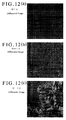
- the concrete processing is simpler in binary pictures than in continual-tone pictures. An example of processing a binary picture is explained by referring to Fig.3.
- Fig.3 exhibits the steps of processing an original binary Chinese character printed in the Gothic font.
- Fig.3(a) is an original picture. The character is written in black on a white background. The tones of the white region and the black regions are constant. The object picture is read-in by an image scanner in quite the same manner as the continually tone-changing pictures. This method deduces the regions of the pixels having similar tones, paints the regions with an average tone of the regions, and memorizes the average-tone image in the region memory-device.
- the boundaries are just equal to the outlines of the character.
- the average tone within the outlines is equal to the uniform tone of the black regions. All the outlines are independent, isolated and separated from others. The outlines have neither crossing points nor branching points. There is no boundary which divides the binary picture into more than two regions. There is no branch point at which three or four different regions are in contact. Non-existence of the branch point, separated outlines, two valued regions and a monotone of the regions simplify the treatment of binary pictures.
- Fig.3(b) is an average-tone image stored in the region-memory device. The average-tone image is similar to the original picture of Fig.3(a).
- Fig.3(c) shows the boundaries which are just the outlines of the black parts in the binary pictures.
- Fig.3(d) is the figure after the step of extracting branch points. Since the outlines include no branch point, the extraction of branching points has no effect on the figure. Thus Fig.3(d) is equal to Fig.3(c).
- Fig.3(e) shows the step of extracting the turning points on the outlines.
- the turning points are denoted by black dots.
- the subtracted image is calculated by subtracting the average-tone image (Fig.3(b)) from the original picture (Fig.3(a)). Since the average-tone image is equal to the original picture, the differential image is grey in an overall plane.
- Fig.3(f) shows the differential image with grey.
- a differential tone is made by adding the fluctuation tones to the middle tone (L/2). Without fluctuation, the differential image is monotonous grey.
- the approximation functions denote a simple flat plane, having constant coefficients.
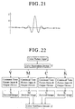
- This invention treats a continual-tone picture by the devices (A) to (X) shown in Fig.1, which will be explained in detail.
- An object picture is drawings, illustrations, characters and so on written on a sheet of paper or photographs having continually-changing tones.
- the object picture is sometimes optically inputted by an image scanner and is resolved to pixels having tone parameters.
- drawings, illustrations or characters are painted on the screen of a computer by a mouse or a digitizer.
- an object picture is supplied in a form of digitally-recorded information by some recording medium, e.g., a floppy disc, a hard disc or a CD.
- some recording medium e.g., a floppy disc, a hard disc or a CD.
- the image memory device 1 (A) is a device for storing the tones of all the pixels of the input picture.
- a pixel In the case of a monochromatic picture, a pixel has only a single tone parameter.
- the steps of tones are, for example, 256, 512 or so.
- the picture In the case of a color picture, the picture should be resolved into four or three elementary-color images. Once the object is resolved by color, the object picture can be reduced to four or three independent monochromatic pictures.
- a pixel has four or three tone parameters. Every elementary color image is a monochromatic continual-tone picture. Then the processes can be reduced to the case of a monochromatic picture.
- the input picture is expressed by a two-dimensional function defined on the whole of the image for giving a distribution of tones.
- the tones of the input picture are given by a continual function f(x,y) defined on the two-dimensional coordinates (x,y).
- the steps of tones are digital numbers, e.g. 256, 512, etc.
- the tone function f(x,y) is now assumed as a normalized function taking a value between 0 and 1.
- the definition range (x,y) may be changed according to the object picture. In this example, the definition range (x,y) is also assumed to be a normalized scope of a square of 1 ⁇ 1.
- an arbitrary continual-tone picture can be represented by the normalized tone function f(x,y) and the normalized definition range (x,y); 0 ⁇ f(x,y) ⁇ 1, 0 ⁇ x ⁇ 1, 0 ⁇ y ⁇ 1.
- the tone f(x,y) and the position (x,y) take continual values in the allowed ranges. These variables, however, take discrete values when the picture is read-in by an image scanner.
- the tone f(x,y) is quantized into L levels between 0 and 1.
- the x-coordinate is also quantized into I dots, and the y-coordinate is sampled into J dots.
- the sampled coordinates are denoted by discrete dots (x i ,y j ), and the quantized tones are represented by g(x i ,y j ).
- L is the number of discrete steps of tone.
- I is the number of pixels in the x-direction
- J is the number of the pixels in the y-direction.
- the image plane has I columns and J lines of pixels.
- the coordinates of pixels are different from the coordinates of boundaries.
- the coordinates of boundaries are taken at the corners of pixels.
- the coordinates of pixels denote the centers of the pixels. Thus both the coordinates differ each other by half a pixel.
- the total number of the pixels is IJ.
- the three size parameters can be freely determined. The bigger these parameters become, the higher the quality of the revived pictures rises.
- the bigger numbers of parameters I, J and L require the larger capacity of memory and the longer processing time.
- the image memory device 1 (A) stores all the digitalized tone parameters of all the pixels, as they are. All the image date must temporarily be memorized in the image memory device (A) before the data compression. Of course, a large capacity of memory is consumed , because the image memory device (A) contains all the image data; all the tones of all the pixels. The image data, however, are erased just when the image data are processed by the steps of the present invention. No memory of the crude image data remains in the memory devices of the computer when the compression process has been finished. Thus the temporary occupation of memories brings about no serious problem.
- Prior image processing methods 1 ⁇ to mentioned before do not divide an input picture into plural regions spatially at all.
- This invention spatially divides a picture into a plurality of regions by the difference of tones.
- the region-division is a quite original way. The regions are neither inherent nor intrinsic to the input picture. The regions here do not correspond to the concrete, individual objects in the picture. The region-division is quite different from the extraction of the outlines of the objects in a binary tone picture.
- This invention forcibly makes the regions which have never existed intrinsically in the picture. Instead of actual objects or matters, this invention finds out imaginary regions on the input picture and divides the picture into separate regions.
- This invention selects the pixels which neighbor with each other and have similar tones as members of a region.
- the criterion of belonging to the same region is the similarity of the tone.
- Two neighboring pixels shall be classified into the same region, if they have similar tones within an allowable tolerance.
- Another two neighboring pixels shall, otherwise, be classified into different regions, if they have different tones beyond the tolerance.
- the continuity of the pixels is essential in the division of the picture.
- the continuity of the pixels ensures the spatial continuity of the regions.
- the division based upon the similarity of tones characterizes this invention.
- the preliminary tone-based division brings about some advantages;
- the average tone is a parameter defined to a region.
- the average tone is a common, single value in a region. But the average tones are different for different regions.
- differences between the tones of individual pixels and the average tone are calculated for all the regions.
- the difference between the tone of the individual pixel and the average tone is called a "differential tone”or a "subtracted tone".
- the average of the differential tones is always 0 in every region.
- the change of the subtracted tones is small and slow.
- the changes of the differential (subtracted) tones can be easily approximated by low order functions for all the regions.
- the above three advantages are essential to this invention. Intrinsic significance of the three features is preliminarily explained now.
- the tones may change at random two-dimensionally in the original picture.
- the change of tones may be smooth and slow at some parts but may be steep and discontinuous at other parts. Since the approximation functions must reflect the change of tones with fidelity, the approximation of steep, discontinuous parts requires high order polynomials which have plenty of parameters.
- the present invention preliminarily divides the picture into a plurality of small regions which have only the pixels with similar tones. The division into regions facilitates the approximation by polynomials for two reasons.
- the picture has been classified into boundaries and regions. Since the imaginary regions have been selected as assemblies of the pixels having similar tones, the boundaries are discontinuous parts. All the parts which have random variations of tone must have been included in the boundaries. In other words, the step of dividing a picture into regions sweeps all the parts having steep changing tones into the boundaries. The boundaries are pitfalls of discontinuous parts.
- the boundaries are singular lines in the tone function.
- the boundaries are assemblies of singular points in the variations of tones.
- the region-division is the most effective way for sweeping discontinuities of tones aside out and gathering them into boundaries.
- an average tone is calculated for every individual region.
- the averages are different for different regions of course.
- the average is a definite value for all the pixels within a region.
- the individual region is painted with the average tone.
- the assembly of the regions painted with the average tones is named an "average-tone image".
- a region all the deviations of the tone of each pixel from the average tone are reckoned.
- the deviation is called a "differential tone" which is defined as a difference between the original tone of the pixel and the average tone of the region.
- the averages of the differential tones are always 0 in every region.
- the subtracted (differential) tones vary slowly and continually in any regions, since singularities have been expelled out of the regions.
- the subtraction tones change so weak and so small that low order polynomials can approximate the subtraction tones with high accuracy.
- the region-division step is important for the present invention.
- the region-division device is a means for dividing an input picture into plenty of small regions which are assemblies of the pixels having similar tones and neighboring with each other.
- the regions and the boundaries are chosen for reducing the tone differences among the pixels within a region but for gathering the discontinuity to the boundaries.
- the assembly of the boundaries and the regions gives three advantages of raising the quality of the revived picture, sharpening the edges, alleviating the number of the data, and shortening the processing time.
- the region-division step of the present invention does not outline the real objects in the picture, but extracts a group of the pixels having similar tones to a region.
- the region-division does not seek for intrinsic regions, but makes forcibly the regions which do not exist inherently, and divides the picture into the imagined regions.
- a region label "Label (x i ,y j )" is allotted to every pixel (x i ,y j ).
- the maximum tone, the minimum tone and the average tone are denoted by g max , g min and g av respectively. Since these are the parameters for regions, the parameter (r) for denoting the number of the region should be suffixed like g max (r) . But the region parameter (r) is omitted here for simplicity.
- the outstanding pixel is now denoted by (x i ,y j ) which belongs to the r-th region.
- the input picture is divided into regions by adopting the concept of "eight-neighbors" which denote eight pixels up and down, right and left, and oblique around the outstanding pixel.
- the operation of the region-division consists of the generation of regions and the determination of the pixels which should belong to the regions.
- the pixel (x i+k ,y j+l ) is labeled and the label function becomes 1.
- Labelling means that the pixel is classified into a region which has a small fluctuation of tones within the tolerance W. If there is a single neighboring pixel which satisfies inequality (6), the operation should be ended for the outstanding pixel (xi,yj).
- g max shall be replaced by g(x i+k ,y j+l ). If g(x i+k ,y j+l ) is smaller than g min , g min shall be replaced by g(x i+k ,y j+l ). Namely, if g(x i+k ,y j+l ) deviates from the present width of tones of the current region, the extremity which is exceeded by g(x i+k ,y j+l ) shall be rewritten by g(x i+k ,y j+l ).
- g max and g min ensures the fact that all the tones included in the current region lie between g min and g max . Since the neighbors satisfy inequality (6), the width of the tones never exceed W, which will be proved later. If g(x i+k ,y j+l ) ⁇ g min , g min shall be rewritten by g(x i+k ,y j+l ). g min ⁇ g(x i+k ,y j+l ). Similarly, if g(x i+k ,y j+l ) > g max , g max shall be rewritten by g(x i+k ,y j+l ).
- g max ⁇ g(x i+k ,y j+l ). If neither (8) nor (9) does not hold, both g max and g min maintain the previous values. Since g max and g min are renewed, the width of tones of the pixels belonging to the current r-th region is widened. However, any pixel once judged as a pixel in the r-th region does not deviate from the values which are determined by inequality (6), because the renewal has a tendency of letting the width between the maximum and the minimum be equal to W.
- An increase of the members of a region enlarges the difference 2U between g max and g min in the region-division step.
- the upper limit of the difference 2U is 2W ( g max -g min ⁇ 2W ).
- the difference (g max -g min ) 2U converges to 2W.
- some regions have the final difference equal 2U to 2W.
- other regions have the final difference 2U smaller than 2W. In any cases, the difference (g max -g min ) never deviates from the width 2W.
- the division of regions is not uniquely determined.
- the region-division depends on the order of the classification step. Since there are a plurality of pixels neighboring to an outstanding pixel (xi,yj), the region with which a neighboring pixel is associated depends on the order of labelling.
- the central pixel (xi,yj) is denoted by C.
- Two neighboring pixels of C-pixel are denoted by D and E.
- C-pixel has a tone g.
- D-pixel has a tone of e.g., g+0.9W
- E-pixel has another tone of e.g., g-0.9W. If D-pixel is classified into a region earlier than E-pixel, the average of the region is raised up to g+0.45W.
- E-pixel cannot join the current r-th regions, but is classified to another region.
- C-pixel and D-pixel are classified into the same region.
- E-pixel is affiliated to another region.
- the average g av is revised to g-0.45W. The fall of the average refuses the affiliation of D-pixel to the r-th region.
- C-pixel and E-pixel are associated with the same region.
- D-pixel belongs to another region.
- the region-division is unique, because the order of labelling is predetermined. Namely, the predetermination of the order of labelling determines the assortment of pixels into regions. If the order of labelling were varied, the assortment of pixels would be changed as a matter of course. The fact clarifies that the region-division does not extract inherent, intrinsic features from the input picture. The regions do not correspond to intrinsic objects.
- the tone difference between D-pixel and E-pixel is 1.4W, but D-pixel and E-pixel belong to the same region.
- the tone difference between E-pixel and F-pixel is only 0.4W, but F-pixel is separated from E-pixel.
- the boundary traverses not the steepest gradient but a modest gradient. Such an unreasonable division results from the assortment of pixels depending upon the tone difference from the average tone by inequality (6) instead of differentiating the tone functions two-dimensionally.
- region-division of the present invention differs from such an intuitive, natural division by human eye-sight.
- Steps 1 to 3 affiliate all the neighboring pixels (x i+k ,y j+l ) satisfying (6) into the same region of the current pixel (x i ,y j ). Then the current pixel shall be transferred to one of the neighbors (x i+k ,y j+l ). Thus (x i ,y j ) ⁇ (x i+k ,y j+l ). Step 3 is repeated to the new current pixel. The repetitions of Step 3 for the neighbors satisfying (6) make up a continual region consisting of the pixels having similar tones.
- Step 3 the next (r+1)-th region shall be made by repeating Step 3 from the last neighboring pixel which does not satisfy (6).
- the regions have all been found out by repeating Step 2 to Step 4.
- the parameter W is a common width of the allowable tones in every region. The bigger the width parameter W is, the wider the regions are. The existence of wider regions requires a longer time for processing the regional data. On the contrary, a smaller width W increases the number of regions and the time for extraction of regions. The smaller W is liable to decrease the time of approximating the regions by the functions.
- the selection of W changes the mode of the region-division.
- Every region is uniformly painted with the average tone "h" of the pixels belonging to the region.
- the average tone h is a true average which is obtained by summing up the tones of all the pixels of the current region and dividing the sum by the number of the pixel in the region unlike the previous average g av which is a mean value of g max and g min .
- "h" is defined independently for every region.
- the average-tone h is a constant within a region irrespective of individual pixels in the region. Since h is a tone variable, h takes any one of 0, 1, 2, 3, ⁇ , and L-1.
- the average-tone is a parameter of a region.
- the number (r) of the region should be suffixed to h. But the expression of the region number (r) is omitted in h.
- the boundary-extraction device carries out the step of seeking the boundaries between neighboring regions. Since all the regions have been determined by the region-division device (B), the boundaries have been predetermined at the same time. The boundaries must be clearly extracted as the lines between the neighboring regions, because the boundaries will be expressed by functions at a later step. Unlike the outlines of binary pictures in conventional image processing methods, the boundary of the present invention is not an assembly of pixels . A series of pixels does not mean a boundary. The boundary requires a new definition in the present invention.
- Fig.5(a) shows the coordinate defined on the input image.
- Fig.5(b) is an enlarged part in the vicinity of the origin (0,0).
- X-coordinate (abscissa) horizontally expands from the origin to the right.
- Y-coordinate (ordinate) vertically extends from the origin to the bottom.
- the choice of the coordinate system has two advantages.
- One advantage is that the (integer) coordinate points can be the boundaries between regions.
- the other merit is that a point consisting of a single pixel or a line of a single pixel width can be treated as a region having a definite area instead of an infinitesimal area.
- the first advantage is quite convenient for defining and determining the boundaries.
- the region-division (B) divides all the pixels into some regions. Every pixel is allotted to some region. No pixel is left for boundaries. In other words, the boundaries can include no pixel.
- the definition of the boundary itself is novel and singular. If the centers of pixels were to be the coordinate points, a series of pixels must have been allocated to boundaries. Some pixels would define regions and other pixels would depict boundaries. The boundaries could not exactly be determined by the prior definition of the coordinate system.
- the second advantage is effective in enlargement, reduction or transformation. If the centers of pixels were to coincide with the coordinate points, a spot of a single pixel or a line of a single pixel width would be expressed as a point or a line without a definite area. If the point or the line were enlarged, the enlarged spot or line would have still a width of a single pixel, because an infinitesimal value is still infinitesimal even if it is multiplied by some definite number. Thus the enlargement would be anisotropic for the lines having a single pixel width.
- this invention takes the corners of pixels as the coordinate points.
- the spot of a dot (pixel) or the line of a dot width is also a region having a definite area, which is suitable for enlargement or other transformation of the image.
- Fig.6 demonstrates the difference of enlargement between the two coordinate systems.
- An original figure is a direct line consisting of nine aligning pixels as shown by Fig.6(a). If the integer coordinate points are allocated to the centers of pixels (Fig.6(b)), an enlarged line is still a line having the same single dot width, although the length is multiplied by the enlargement rate as exhibited by Fig.6(c). This is because the original line Is represented by 0 ⁇ 9. If the coordinate points are allotted to the corners of pixels (Fig.6(d)), the original line is a rectangle having an area of 1 ⁇ 9.
- the line can be isotropically enlarged to both the direction of length and the direction of width, as shown in Fig.6(e).
- the choice of the coordinate system of Fig.5 is effective for enlargement or reduction with fidelity.
- Such a choice of the coordinates is also one of the novel, characteristic points of the present invention.
- This invention denies the prior coordinate system which has a tendency of confusing pixels with coordinate points owing to the coincidence of centers of pixels with the coordinate points.
- the whole of the input picture has been divided into regions by the steps explained hitherto.
- the data of the regions must be compressed for sparing the capacity of memories and facilitating the calculations.
- the minimum elements for defining the regions clearly are outlines of the regions.
- the whole of the input image is divided into regions and all the regions have outlines. There is another region outside of the outline. Thus an outline of a region should be rather called a "boundary" between regions.
- the regions are easily defined by the boundaries. Therefore, the regional data can be compressed by extracting the boundaries and expressing the boundaries by a small number of parameters.
- the boundaries are series of discrete boundary points.
- the boundary point series are a set of the (integer) coordinate points which are connected in four directions; up and down, right and left, on a boundary. Since the coordinate points are defined as corners of pixels, the four-linkage mode of connection is natural.
- the four-linkage neighbors of (m, n) are (m+1,n), (m-1,n), (m,n-1) and (m,n+1). The distance between two neighboring points is always equal to the side of a pixel.
- R denotes the total number of regions.
- N(r) is the total number of the points on the boundary enclosing the r-th region.
- the pixels of the r-th region are extracted from the data stored in the region-memory device (C).
- An arbitrary point on the boundary of the 0-th region is found out, for example, by the raster scanning of the pixels.
- the point series are traced clockwise on the boundary of the 0-th region from the point as an initial point (x 0 (0) , y 0 (0) ).
- the chain code method can be applied to the tracing of the boundary point series.
- the boundaries are closed loops which are not separated from each other, but are in contact with each other.
- the boundary often has the points at which more than two boundaries meet.
- the point at which a plurality of boundaries bisect is called a "branch point.
- a boundary is clearly different from an outline of a binary image, because an outline has no branch.
- the branch points are one type of the characteristic points on the boundaries.
- the branch point is defined as a point having bisecting boundaries or having more than two regions in contact on a boundary.
- a branch point extraction device seeks the branch points on the boundaries. The extraction of branch points is important.
- the branch points give one type of end points to the lines which are approximated by the pertinent functions.
- the branch points are sought by scanning a (2 ⁇ 2) window on the average-tone image stored in the region-memory device (C) in the raster order.
- Fig.7(a) shows the raster scanning of the (2 ⁇ 2) window having four pixels. Such a window having four pixels determines whether the central point of the window is a branch point or not. If all the four pixels have the same tone, the central outstanding point is not a branch because no boundary exists in the window. At least one pixel must have a tone different from the others for including a boundary within the window.
- the central outstanding point is judged as a non-branch point, because a branch point requires at least three different regions.
- the (2 ⁇ 2) window includes three different tones, as shown in Fig.7(c)
- the central point is judged as a branch point. If the window contains four different tones, the central point is also a branch point.
- the boundary interval is a unit of the function approximation. Every boundary interval has two branch points at both ends. There is no branch point in the boundary interval except the ends. No intermediate point is a branch point in any boundary interval. When two neighboring regions commonly possess an interval, the boundary interval is numbered with the same number in both regions.
- Fig.8(a) demonstrates an example of an image having five regions with different tones.
- the branch point is a point at which at least three regions gather around. This example has three branch points.
- Fig.8(b) is an enlarged view of the part encircled in Fig.8(a) containing two branch points ( ⁇ ) and ( ⁇ ).
- the line ⁇ ⁇ is a boundary interval which belongs to two neighboring regions.
- All the closed boundaries are divided into plenty of boundary intervals by cutting the boundaries at the branch points.
- P is the total number of boundary intervals on the input image.
- M(p) is the total number of serial points in the p-th interval.
- x k (p) is x-coordinate of the k-th point in the p-th boundary interval
- y k (p) is y-coordinate of the k-th point in the p-th boundary interval.
- a boundary turning point is defined as a point on a boundary at which the gradient of the boundary changes drastically.
- the boundary turning point is the other important point on the boundary.
- the boundary turning point is shortened to a "turning point".
- the change of the gradient corresponds to a curvature.
- the turning point is a big curvature point in other words.
- the branch points and the turning points characterize the boundaries. This invention further cuts the boundary intervals at the turning points.
- the boundaries are doubly divided at both the branch points and the turning points. It is one of the excellent features of the present invention to divide the boundaries by the branch points and the turning points and to approximate the divided parts by some special functions. Parts of a boundary divided at branch points and turning points are called "subboundaries". Attention must be paid to the difference among a boundary, a boundary interval and a subboundary. Branch points cut a boundary into a plurality of boundary intervals. Turning points cut a boundary interval into a plurality of subboundaries.
- the boundary is the longest in length.
- the subboundary is the shortest among the three. Namely, (boundary) > (boundary interval) ⁇ (subboundary).
- the boundary is a closed loop.
- the boundary interval and the subboundary are lines having both ends.
- the ends of a boundary interval are branch points.
- the ends of a subboundary are branch points or turning points. Since a boundary includes branch points which disturb a serial approximation of the boundary, this invention excludes branch points from the boundary. Since a boundary interval may include strongly-curved points which would invite high order polynomials for approximation, this invention excludes the turning points.
- this invention tries to eliminate vehemently-changing parts as turning points and to approximate smoothly, continually-changing parts by low order functions.
- This approximation has advantages of the low order function approximation, a small number of data, and exact regeneration with high fidelity.
- the present invention succeeds in maintaining the quality of pictures and suppressing the amount of data, since this invention seeks and eliminates the turning points on the boundaries and approximates the subboundaries without singular points.
- the turning points are sought on the boundaries by the following steps.
- a local direction vector is defined at every point on boundary point series.
- the local direction vector is represented as "Direction(p,k)", where p denotes the number of a boundary and k is the number of a point on the boundary.
- Direction(p, k) means the local gradient of the boundary at the k-th point ⁇ (x k (p) , y k (p) ) ⁇ on the p-th boundary.
- the Direction(p,k) of the current point (x k (p) , y k (p) ) is defined as a vector which is drawn from one point (x k-a (p) , y k-a (p) ) preceding the current point (x k (p) , y k (p) ) by "a" unit lengths along the boundary to the other point (x k+a (p) , y k+a (p) ) succeeding the current point by "a" unit lengths along the boundary.
- the unit length is a length of the side of a pixel.
- the dots mean integer coordinate points, that is, the corners of pixels. Boundaries are all defined not on pixels but on dots.
- Direction(p, k): vector(x k+a (p) - x k-a (p) , y k+a (p) - y k-a (p) )
- a means a parameter signifying the locality of the vector.
- the vector spans two points on a boundary separating by 2a unit lengths. The two points (x k-a (p) , y k-a (p) ) and (x k+a (p) , y k+a (p) ) sandwich the current point (x k (p) , y k (p) ).
- the parameter "a” is an integer which should be chosen for extracting the direction of the boundaries in the most suitable way.
- the local direction vector Direction(p, ⁇ ) at ⁇ is an arrow ⁇ ⁇ . Squares mean pixels.
- the corner points correspond to the integer coordinate points (dots).
- the vector does not necessarily cross the current (object) point (dot) but in many cases separates from the current dot.
- Fig.9(b) exhibits an example of local direction vectors along with the boundary.
- the boundary starts from the upper, leftest dot, runs to the right, turns down at dot ⁇ , turns to the right at dot ⁇ , rises at dot ⁇ , turns to the right at ⁇ , turns down again at ⁇ and so forth.
- This process quantumizes the local direction vectors into eight directions of a width of 45 degrees by the slanting angles.
- the direction space of the vectors is divided into eight fan-shaped areas defined by the radius of angles of -22.5° , +22.5° , 67.5° , 112.5° , ⁇ , and 292.5° slanting to the x-direction.
- the fan-shaped areas are called by the average inclining degrees.
- the area between -22.5° and +22.5° is named 0° fan-shape area.
- Another area between +22.5° and 67.5° is named 45° fan-shape area.
- Another area between 67.5° and 112.5° is 90° fan-shape area.
- the other area between 247.5° and 292.5° is 270° fan-shape ares.
- the vectors included in the same fan-shaped area are deemed to be the same vector.
- new vectors are again attached with an angle which is an average on the fan-shape areas. For example, if the inclining angle ranges from 247.5° to 292.5° , 270° is assigned to the vector.
- the quantization aims at stabilizing the local directional vectors against noise.
- the quantized local direction vector is called a "directional vector" and is represented as Direction(p,k).
- Fig.10 shows an example of directional vectors which have been obtained by quantumizing the local direction vectors of Fig.9(b).
- the length of the directional vectors is normalized to 1.
- the position of the vectors Is also changed.
- the middle points of the directional vectors coincide with the current dots, because only the angle is significant for extracting the turning points.
- the lengths or stating points are less important.
- Quantumization decreases the fluctuation of the directions of the vectors. Most of the vectors are reduced to 0° fan-shaped area and are given with an inclination angle of 0° .
- Vector ⁇ ⁇ which inclines at 18° in Fig.9(a) is reduced to the quantized "0" fan-shaped area and is endowed with an inclination angle of 0 degree.
- Vectors of a 72° inclination is classified to the 90° fan-shaped area and allocated with 90° by quantization.
- Quantumization cuts noise and makes an assembly of simplified direction vectors, as shown in Fig.10.
- the choice of the parameter "a” has an influence on the result of course. Too long “a” causes insensitivity to the local change of direction of the boundaries. Too short “a” results in misoperation due to noise.
- the local turning angles ⁇ (p,k) are reckoned at all series of dots on all the boundary intervals.
- the local turning angle ⁇ (p,k) on a dot ⁇ (x k (p) , y k (p) ) ⁇ of a boundary interval is defined as a difference between a direction vector preceding the current dot by b unit lengths and another direction vector succeeding the current dot by b unit lengths.
- the local turning angle is defined by the inner product of the b-preceding vector and the b-succeeding vector divided by the product of the lengths of the vectors.
- ⁇ The definition range of ⁇ is - ⁇ ⁇ ⁇ ⁇ ⁇ .
- Eq.(12) cannot decide whether ⁇ is positive or negative, because cosine function is an even function regarding ⁇ . Then an extra condition gives the sign of ⁇ . If the curve is a clockwise curve along the point series of a boundary, ⁇ is defined as positive. If the curve is a counterclockwise curve along the point series of the boundary, ⁇ is defined as negative.
- Eq.(12) includes not the Direction of the current dot itself, but includes the Direction vector at the (k-b)-th dot preceding the current dot (k-th dot) by b dots and the Direction vector at the (k+b)-th dot succeeding the current (k-th) dot by b dots.
- b is a parameter representing the locality in the determination of the turning of the boundary. If b is too small, the turning angle ⁇ cannot reflect wide-range changes of the boundaries. If b is too big, the turning angle ⁇ omits localized changes of boundaries.
- ⁇ is a parameter which is predetermined to be a constant value between - ⁇ and + ⁇ for determining the degree of turning points.
- Turning angles may be defined by another simpler way. If a turning angle ⁇ (p,k) were defined to be a difference of the inclination angles of the neighboring vectors, the sum of the turning angles ⁇ (p,k) would be always equal to the inclination angle of the current vector.
- the simple method would deem also the curving dots ( ⁇ ), ( ⁇ ), ( ⁇ ), and ( ⁇ ) to be turning points. But the dots ( ⁇ ), ( ⁇ ), ( ⁇ ) and ( ⁇ ) are not true turning points.
- the dots ( ⁇ ), ( ⁇ ), ( ⁇ ), and ( ⁇ ) must be eliminated posteriorly by some means. This invention need not such a step, since the dots ( ⁇ ), ( ⁇ ), ( ⁇ ) and ( ⁇ ) are not deemed as turning points from the beginning. This invention does not employ such a simple definition for the reason. Such a simple sum rule mentioned before does not hold in this invention.
- the preceding steps have extracted boundaries, branch points and turning points on the boundaries.
- the boundary intervals have no more branch.
- the boundary intervals have been divided into subboundaries at the turning points, the subboundaries have no more turning point which has a big curvature. Namely, a boundary is divided into a plurality of boundary intervals at the branch points, and a boundary interval is again divided into a plurality of subboundaries at the turning points.
- a subboundary is a regular line without singularity.
- the boundary approximation device (H) approximates the subboundaries by suitable functions.
- the subboundary is a straight line or a smooth curving line, because the turning points with large curvatures have been removed.
- the word "line” means both a straight line and a smooth curving line for the subboundary.
- the ends of a subboundary are either a branch point or a turning point.
- the characteristic points are singular points on the boundaries. Subboundaries have no singular points except both ends.
- the boundaries and the characteristic points have been extracted by the preceding steps.
- the boundary which is an assembly of points is given by a set of coordinates of series of points.
- a vast amount of the data, as they are, would consume great many bits of memories.
- enlargement, reduction, rotation, parallel displacement or other transformation is difficult to practice directly on the assembly of the crude data.
- This invention does not adopt such an inconvenient way of memorizing data. Otherwise, this invention tries to compress the data of the boundaries for alleviating the burden of memories and for allowing the enlargement or other transformation.
- the coordinates of the characteristic points must be memorized in any way. It is, however, possible to reduce the quantity of the data by approximating the intermediate point series on the lines (subboundaries) between two neighboring characteristic points.
- the subboundaries sandwiched by two characteristic points are moderately-curving lines or straight lines which can be approximated with low order polynomials.
- Spline functions are a set of piecewise polynomials which are often used to interpolate random-distributing points. The points at which the polynomials change are called "knots.” Every interval between the neighboring knots is expressed by a different m-th order piecewise polynomial. Two neighboring m-th order polynomials have the same value, the same first order differential, ⁇ , and the same (m-1)-th order differential at a knot. But the m-th order differential is discontinuous at the knot.
- the spline interpolation can raise the accuracy by dispersing knots at pertinent positions. It is one of the conventional skills of the spline approximation to seek the optimum positions of knots suitably for raising the accuracy.
- T denotes the length of a subboundary.
- Piece number "M” is a new parameter for denoting the number of pieces. Namely, the subboundary T is equally divided by M into pieces of a length of (T/M). The knots are assumed to be distributed uniformly on the points separated on the subboundary by a length of (T/M). T and M determine automatically the positions of knots. T, the length, depends on the current subboundary. M is a freely-determinable parameter which gives the positions of knots. The accuracy of approximation can be heightened by increasing M.
- the spline functions this invention adopts are a kind of normalized B-splines.
- the knots are given a subboundary at the points separated by a length (T/M).
- the division number M and the dimension m are the parameters for determining the spline functions.
- M is the number of dividing a subboundary.
- the divided lengths are called "pieces".
- Individual pieces are designated by suffixes k, l and so on.
- the approximation uses a set of spline base functions (or spline bases in brief).
- a spline function is a localized function given as a sum of several polynomials.
- the approximation of the present invention represents an arbitrary curve by a linear combination of the spline base functions.
- M is the number of the pieces defined on a subboundary. M is called a division number, since a subboundary is divided into M pieces.
- the dimension "m” is the order of the spline bases. Namely, the highest order of the terms of the base polynomial is m.
- the integration is 1, since it is normalized.
- the m-th spline base is an m-th order polynomial ranging over (m+1) pieces.
- the m-th order spline is often called the (m+1)-th rank spline which is represented as N q, m+1 .
- N q, m+1 is simply written as N q by omitting (m+1).
- ⁇ is a length of piece.
- the previous steps have removed branch points and turning points from boundaries and have prepared subboundaries which contain no characteristic points except both ends.
- the subboundaries include low frequency components. Low dimension functions are sufficient to approximate the subboundaries.
- the base N 0 (t) has a positive, round peak ranging in three pieces.
- the base N 0 (t) can be represented by simple quadratic polynomials; (a) 0 ⁇ t ⁇ 1 t 2 /2 (b) 1 ⁇ t ⁇ 2 (3/4)- ⁇ t-(3/2)) ⁇ 2 (c) 2 ⁇ t ⁇ 3 (t-3) 2 /2.
- N 0 (t) 0.
- the 2nd rank differential d 2 N 0 /dt 2 is discontinuous there.
- N 0 (t) is normalized for yielding 1 by integration.
- the 2nd order spline is the simplest among the spline functions having smooth curving lines. Fig.20 exhibits the areas of parts of N 0 (t).
- the functions which are defined at all the pieces but are different polynomials at different pieces are called "piecewise polynomials".
- the second order spline is the simplest in the spline functions which can represent curves. It is a matter of course to build up this invention on the basis of third order splines. However, this invention will be described hereinafter on the framework constructed by the second order spline bases.
- a boundary is intrinsically a continual line.
- the boundary which this invention defines is a series of points which are the corners of pixels.
- the boundary is a set of continually neighboring points.
- the eight-neighbor approach joins a central point with another point among eight neighboring points.
- the four-neighbor approach couples a central point with another point of four neighboring points. Since the boundary is defined at the corners (dots) of pixels, the eight-neighbor approach is not suitable, since the chains connecting dots would cross over the pixels.
- this invention joins the points on boundaries by the four-neighbor approach.
- the points on a boundary is called a boundary point series.
- the total number of points is denoted by "n”.
- the k-th point (0 ⁇ k ⁇ n-1) is denoted by (x k , y k ).
- a boundary is represented by a set ⁇ (x k , y k ) ⁇ of the continually joining points.
- the image memory device still maintains all the data of ⁇ (x k , y k ) ⁇ at the present step.
- the amount of the data is too large. It is desirable to memorize the regular subboundaries by a smaller amount of memory through some interpolation technique.
- the interpolation by spline functions has been explained hereinbefore.
- the subboundaries cannot be approximated by the spline functions, because the subboundaries are two-dimensional variables.
- the number "k” determines the order of the point series and gives a tight connection between x k and y k of the k-th point.
- the intermediate, independent variable is "t”. All the points k of a subboundary are allocated to some values of t. "t k " is the value allotted to the k-th points. "t k " is a function uniformly increasing with k. The combination of ⁇ t k ⁇ with ⁇ (x k ,y k ) ⁇ makes two sets of coordinates ⁇ (t k , x k ) ⁇ and ⁇ t k , y k ) ⁇ for the point group ⁇ k ⁇ .
- t k is a monotonously-rising function of k
- x k and y k are single-valued functions of t.
- the property enables spline functions to approximate ⁇ x k ⁇ and ⁇ y k ⁇ .
- ⁇ x k ⁇ shall be approximated by s x (t), and ⁇ y k ⁇ shall be approximated by s y (t).
- the function sx(t) is a linear combination of the spline bases ⁇ N q (t) ⁇ with coefficients ⁇ c xq ⁇ .
- the function s y (t) is given by a linear combination of the spline bases ⁇ N q (t) ⁇ with coefficients ⁇ c yq ⁇ .
- N q (t) is a mountainous function localized in [q, q+3] as shown in Fig.20. The localization is signified not by t but by q in N q (t).
- the intermediate variable "t” takes continual values. At the k-th point on the subboundary, t takes "t k ". But t takes other continual values except t k . Since t is a continual variable, s x (t) and S y (t) can be differentiated by t. The k-th point coordinates are approximately given by s x (t k ) and s y (t k ). However, s x (t k ) and s y (t k ) are not necessarily equal to x k and y k , since s x (t) and s y (t) are approximating functions.
- the determination of the approximating functions is equivalent to determining the coefficients ⁇ (c xq , c yq ) ⁇ .
- the least square error method is the least square error method.
- the other is the "biorthonormal function method" which has been proposed by this Inventor for the first time. The latter can calculate the coefficients in a far shorter time than the least square error method.
- the Inventor believes that the biorthonormal function method contrived by the Inventor is far superior to the least square error method. Since the coefficients can be reckoned by both methods, both the least square error method and the biorthonormal function method will be explained.
- the least square method determines the coefficients ⁇ c xq , c yq ⁇ by calculating the difference between x k and sx(t k ) and the difference between y k and s y (t k ), squaring the differences, summing the differences up, and minimizing the sum.
- the sum of the squares of the differences at all the points is denoted by a square error "Q".
- Q is given by
- k denotes a point on the subboundary, taking the values 0, 1, 2 , ⁇ and n-1.
- the coefficients in s x (t) and s y (t) are determined for minimizing "Q".
- the least square error method is named after the technique of minimizing the square error.
- Eq.(19) and Eq.(20) contains two kinds of summations ( ⁇ ).
- ⁇ of k is a sum of the n points on the current subboundary.
- ⁇ of q is a sum of the (M+2) spline base functions.
- the spline bases are known functions.
- (x k , y k ) are also known.
- ⁇ c xq ⁇ and ⁇ c yq ⁇ are unknown parameters. When c xq and c yq were changed by infinitesimal amounts, Q would always increase in any case, if Q has taken the minimum value.
- the equations are solved for some M. If the result does not satisfy the predetermined criterion, the division number M is increased one by one to M+1. Solving the equations and examining the results are repeated till the result suffices the criterion.
- matrix operation can determine the coefficients.
- t N means a transposed matrix of "N”.
- t N is an n-line, (M+2)-column matrix.
- These matrixes determine c x and c y , because x and y are known vectors and N x and N y are known matrix.
- the product t N x N x is an (M+2) ⁇ (M+2) square matrix which has an inverse matrix ( t N x N x ) -1 .
- Eq.(31) is not an equation for the least square error method but an equation for the criterion. Although Eq.(31) slightly resembles Eq.(21), the meaning of Eq.(31) is entirely different from Eq.(21).
- Eq.(21) is a starting definition for practicing the least square error method for calculating c xq and c yq .
- Eq.(31) gives a criterion for examining whether the calculated c xq and c yq can approximate the subboundary with fidelity.
- the maximum error ⁇ in Eq.(31) is compared with a predetermined value which is a measure of the degree of the approximation. A smaller ⁇ would bring the approximation data s x (t k ) and s y (t k ) closer to the original data (x k ,y k ). But a smaller ⁇ requires more times of repetitions of approximation, which wastes longer time.
- the critical value of ⁇ should be predetermined for reconciling the calculation time with the fidelity of regeneration.
- 0.5 may be chosen as the critical value.
- the approximation steps will be repeated by raising M by 1 as long as ⁇ ⁇ 0.5.
- ⁇ ⁇ 0.5 the approximation step is ended and the current coefficients are employed as the final coefficients.
- the criterion ⁇ ⁇ 0.5 aims at rigorous regeneration with high fidelity.
- the critical value can be predetermined to be a value larger than 1.
- a large critical value reduces the time of calculation. Besides the saving of time, such a larger critical value is suitable for regeneration of smoother boundaries.
- the critical value should be determined in accordance with the purpose.
- the set of sine functions and cosine functions has an ideal orthonormality.
- Bessel functions J m (t) have a special orthonormality. Bessel functions lack periodicity, and have infinite zero-points. The orthonormality takes such a strange form.
- Eq.(34) is not a definite integration but an indefinite integration.
- the coefficients can be reckoned by the orthonormality given by Eq.(34).
- Hermite polynomials Hp(t) are endowed with a plain orthonormality.
- some unknown function series have orthonormality.
- a product of two different eigen functions yields zero by the integration from minus infinity to plus infinity
- the eigen functions ⁇ p (t) ⁇ have simple orthonormality due to the difference of the eigen values E p , either if ⁇ p (t) is known or if ⁇ p (t) is unknown.
- Orthogonality lacks for the spline function bases of any order.
- the integration of the product of two spline bases N q (t) and N p (t) is not zero at all.
- the spline functions do not form an orthonormal function system.
- the assembly of the spline functions is a non-orthonormal function system.
- the spline functions are rather rare functions. What deprives the spline functions of orthonormality?
- Higher order spline, e.g., 3rd order or 4th order, functions have the feet with weak oscillation. The oscillation at the feet is too weak to cancel the integration of a product of different parameter bases.
- the spline functions are artificial functions which were contrived to interpolate discrete points by smooth curves with oscillation as little as possible. Thus it is a matter of course that the spline functions are lacking in oscillation.
- the weak oscillation is equivalent to the discontinuity of the m-th order differential at knots of the m-th order spline functions.
- the m-th spline is a C (m-1) class function which can be differentiated till (m-1) times, but cannot be differentiated more than (m-1) times.
- the spline functions are not infinite time differentiable functions. On the contrary, infinite time differentiations are fully possible on the sine functions, cosine functions, Legendre's functions, Hermite functions and the solutions of Schroedinger equation explained as the examples having orthonormality. Feasibility of the infinite time differentiations gives these functions strong oscillation. Orthogonality originates from the strong oscillation.
- the m-th order spline function is incapable of the m-th time differentiation for the purpose of suppressing oscillation.
- a simple hill-shape facilitates the calculation. But a difficulty arises from the simple hill-shape through the loss of orthonormality.
- Eq.(41) signifies an ideal form of the artificial, orthonormal function. What is the orthonormal function? Can such a set of orthonormal functions exist on earth? Aside from the problem of existence, the artificial function L q (t) is called a "biorthonormal function" of N q (t). The biorthonormal function must suffice the orthonormality
- Eq.(42) is requisite is understood by substituting Eq.(40) into Eq.(41).
- the definite integration of a product of two functions is sometimes called an inner product from an analogy of vector operation.
- the inner product is zero is equivalent to the fact that two functions are orthonormal. Since spline bases are non-orthonormal functions, the inner product of the splines of N p (t) and N q (t) having different parameters p and q respectively has a definite value which is denoted by g pq The inner products g pq can be calculated. Including the division number M, g pq is a function of the difference (p-q). The scope of (p-q) is narrow, because N q (t) or N p (t) is a localized function which occupies only (m+1) pieces.
- the inner product g pq has a definite value for the difference (p-q) between -m and +m (-m ⁇ (p-q) ⁇ +m).
- the assembly of the inner product of spline bases can be deemed as an (M+2) ⁇ (M+2) square matrix G.
- a convenient character of the spline inner product matrix G is that all components of G are known for any M by Eq.(44) to (47), whenever the division M changes. When M is increased to (M+1) for improving approximation, the matrix G is immediately given by the memory without calculating the components.
- the spline inner product matrix G is always a known matrix for arbitrary M.
- Another convenient character of G is the feasibility of reckoning an inverse matrix G -1 , because G is a symmetric matrix.
- An arbitrary function can be represented by a linear combination of the spline base functions ⁇ N q (t) ⁇ in the definition interval [0, T].
- the biorthonormal function L p (t) itself can be represented by a linear combination of ⁇ N q (t) ⁇ with coefficients ⁇ d pq ⁇ , Substitution of Eq.(48) into Eq.(42) yields The integration of the product N s (t)N q (t) is g sq in Eq.(43). Eq.(49) becomes A set of the expansion coefficients ⁇ d ps ⁇ can be deemed as components of an (M+2) ⁇ (M+2) square matrix D.
- the set of the inner products ⁇ g sq ⁇ forms the square matrix G.
- Kronecker's ⁇ makes an (M+2) ⁇ (M+2) unit matrix I .
- the coefficient matrix D is given by an inverse of the spline inner product matrix G.
- D G -1 .
- the components of G have been given in Eq.(44) to Eq.(47) definitely.
- D can easily be calculated from G.
- coefficient matrix D is also a known matrix for any M, which is a very convenient property.
- the matrix operation can be applied to approximate the subboundaries by the spline functions.
- the relation between the spline bases N q (t) and the biorthonormal L q (t) is further clarified.
- the spline base N q (t) is a simple, tranquil function with little oscillation.
- the 2nd order spline base has no oscillation as shown in Fig.20. Even higher order splines have poor oscillation.
- the biorthonormal function L p (t) is a rapidly-changing function accompanied with strong oscillation which is required for cancelling the tranquil N p (t) in the product L p (t)N p (t).
- the inner product of L p and L q is denoted by J pq .
- a matrix J can be constructed by the set of ⁇ J pq ⁇ . J is now called an orthonormal inner product matrix.
- a coefficient matrix U is built with the set of coefficient ⁇ u pq ⁇ .
- Eq.(58) says that the orthonormal inner product matrix J of (Lp ⁇ Lq) is equal to the biorthonormal coefficient matrix D of ⁇ d pq ⁇ which are coefficients on N q , when L p is expanded on ⁇ N q ⁇ .
- Eq.(59) says that the spline inner product matrix G of (N p ⁇ N q ) is equal to the spline coefficient matrix U of ⁇ u pq ⁇ which are coefficients on L q , when N p is expanded on ⁇ L q ⁇ .
- the coefficient of the expansion of the subboundaries are reckoned by the biorthonormal function method instead of the least square error method.
- the k-th point coordinate (x k , y k ) has been divided into (t k , x k ) and (t k , y k ) on the intermediate variable representation.
- the approximated subboundary is given by the continual functions s x (t) and s y (t).
- the coefficients ⁇ c xq ⁇ and ⁇ c yq ⁇ are now calculated on the biorthonormal function method.
- the biorthonormal functions express the coefficients as The coefficients cannot be directly calculated yet, since s x (t) and s y (t) are still unknown. However this fact causes no problem.
- Known date are (t k , x k ) and (t k , y k ).
- the coefficients can be reckoned from the spline bases ⁇ N q (t) ⁇ .
- the matrix ⁇ d qp ⁇ is the inverse matrix of the spline inner product matrix ⁇ g pq ⁇ .
- ⁇ d qp ⁇ are known values for all possible M.
- Np(tk) is obtained from the table memory.
- ⁇ T/M
- T is the full length of the subboundary
- M is the division number of pieces
- ⁇ is the unit length of a piece.
- the biorthonormal function method based upon Eq.(62) and Eq.(63) or Eq.(64) and Eq.(65) is far superior in calculating the coefficients to the least square error method realized by Eq.(29) and Eq.(30) or Eq.(25) and Eq.(26).
- this invention can be carried out by the least square error method.
- this invention prefers to the biorthonormal function method which can greatly shorten the time of calculation.
- the biorthonormal function method obtains 2(M+2) coefficients. Then the degree of the approximation is estimated by the same way which has already been clarified for the estimation of the results brought about by the least square error method.
- the estimation way requires that all the distances between the original points (x k , y k ) and the approximated points (s x (t k ), s y (t k )) must be smaller than a predetermined critical value.
- the maximum of the distances is denoted by ⁇
- the critical value is a parameter which can be freely determined In accordance with the purpose. For instance, when the critical value is settled to be 0.5, the result is examined by inequality ⁇ ⁇ 0.5.
- the approximation of the subboundaries by the spline functions has been fully explained.
- the spline function approximation is competent enough for approximating the regions which are a posteriori yielded of continually-changing tone pictures.
- the same approximation can be applied to binary tone pictures which consists of only two colors, e.g., black and white, of course.
- binary tone pictures inborn outlines of images become boundaries.
- more rigorous regeneration of the boundaries is required. For the purpose, it may be advantageous to extract straight lines, circles and arcs from the assembly of the boundaries and to express them by another function.
- the region data memory device (I) stores many attributes as the region data;
- (1) means the horizontal length and the vertical length of the input picture which requires 4 bytes, as shown in table 1.
- (2) denotes the number of the regions divided by the region-division device (B). The number depends on the substance of the input picture. It needs 2 bytes of the memory.
- (3) is the average tones of all the regions which have been calculated by the region-division device (B) and been memorized in the region memory device (C).
- K1 denotes the number of the regions now. Every region has an average tone. (3) requires K1 bytes for the memory.
- the boundary information (4) determines the relation between the regions and the subboundaries.
- the regions have been numbered and the subboundaries have been numbered.
- a region is enclosed by a plurality of subboundaries.
- a subboundary is in contact with two regions on both sides. Some information must be given for clarifying the relation between the regions and the subboundaries.
- the boundary information contains two kinds of parameters. One is the numbers of the subboundaries enclosing a current region. The other is the directions of the boundaries with regard to the region.
- the direction of a subboundary is not a concept which can easily be understood.
- the direction of a subboundary determines which side of the subboundary the region exists. Every region has a number but has no coordinates for specifying Its position. The boundaries have their own coordinates for specifying the positions. Thus the regions cannot be specified by themselves.
- the position of the regions must be determined through the relation to the subboundaries enclosing the current region. It is important to determine which side of the subboundary the region exists.
- a region can uniquely defined by the subboundaries enclosing the region and the directions of the region with regard to the boundaries.
- the boundary information requires 4K1 bytes.
- a boundary is a closed loop enclosing a region completely.
- a boundary is divided into several boundary intervals by the branch points.
- a boundary interval is divided into several subboundaries by the turning points. (5) needs 4 bytes for being memorized.
- (6) shows the starting points and the division number M for approximation of all the subboundaries.
- K2 denotes the number of subboundaries.
- (6) needs 8K2 bytes.
- (7) means the concrete values of the coefficients ⁇ cxq ⁇ and ⁇ cyq ⁇ on the spline bases for approximating the subboundaries.
- the numbers of the region data are listed in table 1.
- Table 1 shows three categories of information. (1) is the original picture information. (2), (3) and (4) are the region information. (5), (6) and (7) are the boundary information in table 1.
- the original picture has been solved into the regions and the subboundaries. Every region has an average tone. Every subboundary has a concrete locus on the function approximation. What is the remainder? The rest is the information of the individual tones of the pixels in the regions. The average tones cannot fully represent the tone distribution in the original picture, since the average tone is only a single value for a region.
- Fig.2(b) shows an average tone image which gives all the regions their average tones.
- the region-memory device (C) has memorized the Fig.2(b) image, as it is. A region is painted with an average tone h.
- the average-tone image is akin to the original picture of Fig.2(a), since continually-changing tones of the original are converted into stepwisely-changing tones of the average-tone image.
- the average tones in general, represent the tones of the regions pretty well. The degree of the resemblance depends on the tone width W, as explained before.
- the average-tone image is different, in detail tones, from the original picture.
- the average-tone image neglects the local variations of tone within the individual regions, because each region is uniformly painted by an average tone.
- the small fluctuations of tones must be taken into consideration for regenerating the picture with high fidelity.
- the tone of an arbitrary pixel in a region is not necessarily equal to the average tone of the region, but is different from the average tone in many cases. Furthermore, the tones are varying pixel to pixel. A new contrivance is ardently requested now for taking account of the fluctuation of individual tones from the average tone. What suffices the request is the differential image generation device (J) which is explained now.
- the next problem is how to handle the differential tones. It is not a good tactics to memorize all the differential tones of all pixels, as it is, because it would waste too many memories.
- An alternative may be a method of approximating the differential tones within every individual region, because the differential tones are defined within every region, and the regions have been defined by the boundaries. The approximation within regions would, however, be complicated due to the complexity of the boundary conditions, since the boundaries are not regular squares but random closed loops for the regions. It would be difficult to give the boundary conditions to each region. The within-region approximation would be also plagued by a number of data due to the insufficient complicated approximation. Such a large number of data requires a new breakthrough for processing the differential tones.
- this Inventor has hit upon an idea of wide range processing for the fluctuating tones of individual pixels in the regions.
- This Inventor has made a new concept of differential (tone) image for the wide range processing.
- a "differential (tone) image” is imagined as an assembly of all the regions with differential tones.
- the differential tone image is shortened to a "differential image” for simplicity.
- the concept of the "differential image” is one of the most important matters in the present invention.
- the size of the differential image is equal to the size of the input image, since all the regions once divided are unified again into the differential image. Both the boundaries and the regions are seemingly extinct in the differential image.
- the differential image is different from the original image in the tones.
- the "differential image” is defined as an image made by subtracting the average tones from the original, input image.
- a pixel (x i ,y i ) has an original tone g(x i , y i ), and a region has an average tone h.
- the average tone h (r) has been originally defined in a region, the average tone h (r) is also assigned to individual pixels (x i , y i ) belonging to the region (r), as denoted by Eq.(10).
- Fig.2(f) shows a differential image.
- the tones of Fig.2(f) are almost grey, and are far less various than the input image of Fig.2(a). Why does the differential image take grey tones?
- the tones have been quantized in L levels by Eq.(2).
- the base tone of the differential image is L/2.
- Eq.(6) ensures that the fluctuation is less than W in the differential image.
- the tones of all the pixels are restricted in a very narrow scope between (L/2-W) and (L/2+W) which are grey in tone.
- the reason why the fluctuation is very small is that most of the fluctuation has been already removed by the average tones.
- the average-tone image of Fig.2(b) absorbs most of the fluctuation.
- Man can seek a faint shape of the girl.
- the average-tone image of Fig.4(c) gives a far distant impression from the original girl, loosing fine variations of tones.
- W the tone width
- a large W widens the areas of regions.
- the average-tone image deviates far from the original picture.
- the differential image has some features of the original picture.
- a large W decreases the number of regions and the number of boundaries, which alleviates the time of processing of the boundary approximation and the memory of storing the region data and the boundary data.
- a large W has a drawback of a large fluctuation of tones in the differential image.
- the differential image having such a large tone fluctuation requires a plenty of parameters for approximation. Besides the problem of the number of parameters, a large W degrades the accuracy of the approximation. Thus a large W increases the load of approximation of the differential image.
- a small W enhances the number of region data and allocates still more the features to the average-tone image than to the differential image.
- the differential image has almost uniform grey tones due to the poor oscillation of tones. The poor oscillation enables low order functions to approximate the differential image with a small number of coefficients with high fidelity.
- a small W has the advantage of a small number of data and high fidelity regeneration, but suffers from the number of region data and the time of determining the subboundaries. The value of W should be determined for reconciling the region data and the differential image data. In general, a small W can enhance the accuracy of the approximation at the expense of the processing time.
- the differential image memory device (K) stores the differential tones diff(x i , y i ) of all the pixels (x i ,y i ) in the differential image.
- the differential tones could be memorized region by region, because the pixels have been divided into the regions.
- the differential image memory memorizes the differential tones by the pixel number (i, j), ignoring the membership of pixels to the regions.
- the differential image is free from the restriction caused by the regions, the approximation of the differential image is fully immune from the difficulty of the complicated boundary conditions and the enormous regional data.
- the differential image is memorized as the two-dimensional function diff (x i , y i ) of all the coordinates (x i ,y i ) defined on the full scope of the image. Since diff(x i , y i ) has a small fluctuation of tones, low order polynomials can approximate diff(x i , y i ) with little error.
- a further contrivance is proposed here for reducing the time and the data for approximating the differential image.
- the differential image is not partial images, but a single image unifying all the regions. The following steps are irrelevant to the individual regions.
- the differential image has the same size as the original picture, being immune from the division due to the regions.
- the number of vertically-aligning pixels of the original image is denoted by "I”
- the number of horizontally-aligning pixels of the same original image is denoted by "J”.
- the differential image has I vertically-aligning pixels and J horizontally-aligning pixels. Since all the regions have been assembled into a differential image, the differential image has a rectangular shape which is suitable for function approximation.
- the size of the differential picture is equal to the size of the original picture. Isn't there a significant difference between the approximation of the original image and the approximation of the differential image? The approximation of the differential image is clearly different from the approximation of the original picture. Since the original picture includes rough variations, the division number M and the coefficient number would be very large, if the original picture were to be approximated by the same form of functions. Despite a great number of the coefficients, the approximation would be rough and incorrect. The differential image is far superior to the original image for the function approximation.
- the differential image is a special image suitable for the function approximation.
- the uniformity is an important property of the differential image.
- the parts at which the tones change drastically have been eliminated as boundaries from the original image in advance.
- the boundaries absorb the irregular portions.
- the average of the differential image is 0, and the fluctuation is small.
- a further contrivance is required for facilitating the function approximation of the differential image.
- the embodiment thus divides a differential image lengthwise and crosswise into Q small rectangular or square blocks.
- a square block is preferable to a rectangular block, since the processing is symmetric both in x-direction and in y-direction.
- the differential image division device (L) divides the differential image into small blocks for the above reason.
- Fig.13 schematically shows the division of the differential image.
- the differential tones are independently approximated in each of the individual blocks.
- This invention can be carried out without dividing the differential image.
- the division into a plurality of blocks is a contrivance for shortening the time of calculation.
- the differential image can be directly approximated by two-dimensional functions without dividing into blocks.
- the differential tones [diff(x iq ,y jq ) ⁇ Q are stored by blocks in the differential block memory device (M).
- Q is the total number of the blocks.
- the diff(x iq , y iq ) is the differential tone of the i-th point in the q-th block.
- the data approximation device (N) approximates the differential blocks with two-dimensional spline functions.
- the size of the approximation is definite, for example, b ⁇ b in the previous case.
- This is the second approximation in this invention.
- the first one is the one-dimensional approximation of the subboundaries which do not have a definite size.
- the second approximation of the differential blocks is the most important approximation.
- the objects of the approximation have two-dimensional broadness. Thus the differential image shall be approximated by two-variable functions.
- This embodiment adopts two-dimensional spline functions for approximating the tones of blocks.
- three dimensional splines can also be applied to approximate the same differential blocks.
- the differential block is expanded on the two-variable base functions ⁇ mn (x,y).
- the tone distribution in a block is expressed by a linear combination of the spline bases, that is, a sum of the spline bases multiplied by coefficients.
- M is the division number in x-direction.
- N is the division number in y-direction.
- the spline base is given by
- ⁇ + signifies ⁇ when ⁇ ⁇ 0, but 0 when ⁇ ⁇ 0.
- N the division number in y-direction, is different from the base N q (t).
- ⁇ mn (x,y) is a product of one-variable splines N m (x) and N n (y).
- Inequalities (71) declare that the definition range of x and y is [0,1].
- the size of a block is b ⁇ b in the actual image plane. Then the coordinates are here normalized by replacing x by x/b and y by y/b. Thus the definition range is normalized into [0, 1] ⁇ [0, 1].
- the unit width of a piece is 1/M in x-direction and 1/N in y-direction.
- M and N are not necessarily equal, because the degrees of tone variations are, in general, different in the x-direction and in the y-direction.
- the block function is established by determining ⁇ c mn ⁇ since ⁇ mn ⁇ are known functions.
- the coefficients ⁇ c mn ⁇ are calculated by a similar manner to the ways for determining the subboundaries.
- the least square method and the biorthonormal function method are available for identifying the block differential tones. Both methods have been described before as the ways for approximating the subboundaries.
- the biorthonormal function method which has been contrived by the Inventor is superior to the least square method.
- the coefficients ⁇ c mn ⁇ are here reckoned only by the biorthonormal function method.
- the least square method can easily be applied to the differential tone approximation by referring to the previous steps.
- the single-variable spline base N p (x) lacks orthonormality ((N q ⁇ N p ) ⁇ 0), as explained before.
- the two-variable spline base ⁇ mn (x,y) which is a product of N m (x) and N n (y) lacks orthonormality as a matter of course.
- the coefficients ⁇ c mn ⁇ can also be reckoned facilely by defining two-variable biorthonormal functions ⁇ pq (x,y).
- the spline bases ⁇ mn (x,y) and biorthonormal bases ⁇ pq (x,y) satisfy the double orthonormality condition;
- the biorthonormal bases if they exist, the coefficients ⁇ c mn ⁇ in Eq.(73) are briefly represented by
- the biorthonormal base ⁇ mn (x,y) has two variables and two suffixes. Since ⁇ mn (x,y) is a plain product of N m (x) and N n (y), ⁇ mn (x,y) can be determined by a similar manner to the way of seeking L p (x).
- Eq.(81) can be further reduced by the spline bases N p (x) and N q (y) to The reason is briefly clarified.
- the two-variable biorthonormal base ⁇ mn (x,y) is related to two-variable spline ⁇ pq (x,y) by a tensor d mnpq as
- ⁇ pq (x,y) is a direct product of N p and N q
- the tensor d mnpq is a product of d mp and d nq
- d mnpq d mp d nq .
- the set of coefficients ⁇ c mn ⁇ can be calculated either by Eq.(81) or Eq.(82).
- Eq.(82) contains a product of N p (x) and N q (y) which have definite values for very restricted points.
- N p (x i ) has definite values for p/M ⁇ x i ⁇ (p+3)/M , but is zero otherwise. There are three bases having definite values. Thus Eq.(82) has only nine terms having non-zero values. The summation in Eq.(82) is a sum of 9 terms instead of (M+1)(N+1).
- the boundary approximation handles geometric curving lines.
- the tone approximation deals with the tone at every point having definite L steps. The other difference is the variables.
- the boundary approximation uses an intermediate, independent variable t for describing dependent variables (x,y) as functions of t.
- SNR signal noise ratio
- K and H are the lengths in the x-direction and in the y-direction of a block.
- the average of the square of errors is obtained by squaring the errors, summing up the squared errors in the x-direction and in the y-direction and dividing by (K+1)(H+1).
- the average squared error is normalized by dividing by L 2 .
- the inverse of the normalized average squared error is a measure of the accuracy of approximation. The larger the inverse is, the higher the accuracy of approximation rises.
- Eq.(88) includes the inverse of the normalized average squared error in logarithm.
- the SNR has a unit of dB.
- a critical value ⁇ ' is predetermined for estimating the exactness of the approximation. Namely, the approximation of block tones is repeated by increasing M and N to M+1 and N+1 respectively until SNR > ⁇ '.
- the approximation is carried out block by block.
- the purpose of dividing the differential image into blocks and approximating the block tones is to curtail the time of calculation.
- the divisional processing is, of course, optional in this invention. If the restriction on the calculation time can be ignored, it is possible to approximate a full differential image without dividing into blocks as a matter of course.
- the devices and the steps of (L) and (M) should be eliminated, and the step and the device of the differential image memory (K) should be directly followed by the data approximation (N).
- the approximation would be carried out in the wide range of I pixels in the x-direction and J pixels in the y-direction.
- the previously explained way prepares the transformation coefficients ⁇ d mnpq ⁇ which relate the biorthonormal bases to the spline bases and expands the block tones on the spline bases through the biorthonormal bases.
- the matrix D consisting of ⁇ d mn ⁇ is the inverse matrix G -1 of the matrix G constructed by the inner product (N p ⁇ N q ) of two spline bases N p and N q , as shown in Eq.(51) and Eq.(52).
- Eq.(64) and Eq.(65) are suitable equations for calculating ⁇ c xq ⁇ and ⁇ c yq ⁇ without knowing the concrete form of the biorthonormal bases.
- the biorthonormal bases can be directly calculated.
- This Inventor has given a concrete form of the biorthonormal base for the first time on his thesis; T. Horiuchi, "A study on adaptable system model and its application to desktop publishing system", Dissertation, University of Tsukuba, 1995.
- Eq.(90) cannot be analytically integrated, but can be calculated numerically by a computer.
- Fig.21 exhibits the second order biorthonormal base.
- the data approximation device (N) supplies the compressed data of representing the tone distribution in the blocks into the compressed data memory device (O).
- the compressed data include the x-division number M, the y-division number N and coefficients ⁇ c mn ⁇ of every block. Containing the two-dimensional tone data, the compressed data are entirely different from the region data including the information of the characteristic points and the boundaries.
- Table 2 denotes the sizes of the data which are stored in the compressed data memory device (O).
- the encoding is carried out for both the region data of (I) and the compressed data of (O).
- the encoding step reduces the amount of data, but increases the processing time to the contrary.
- the adoption of the encoding step is optional, which should be determined in accordance with the purpose of the image processing. When time should be curtailed, the encoding should be omitted. When memories should be saved, the steps should include the encoding of the once compressed data.
- the encoding device (P) encodes the region data and the compressed data, and the encoding data outputting device (Q) outputs the encoded data in a series of bit signals.
- the encoding is effective not only in compressing the data but also in keeping the secret. Since the data have been encoded by some method, the data must be decoded by the same method for being revived. A third party without the means of decoding cannot recover the data.
- the encoding plays a role of protecting the secrets.
- the encoded data memory device (R) memorizes the encoded information of both region data and compressed data.
- the data stored in this device (R) can be read out at any time according to a request of outputting.
- These devices (A) to (R) are a series of inputting a picture, compressing the image data, storing the region data and the compressed data. These are an earlier half of the image processing. The latter half of the image processing is another series of reading out the data, decoding the data, reviving the image data and outputting the revived picture on some outputting device.
- this invention memorizes fully compressed data by extracting assemblies of pixels having similar tones as regions, painting every region with an average tone for producing an average-tone image, extracting boundaries, dividing the boundaries at branch points and turning points into subboundaries, approximating the subboundaries by the intermediate variable spline approximation, subtracting the average tone image from the input image for making a differential image, and approximating the differential image by two-dimensional spline functions.
- the stored data comprise the region data and the compressed data.
- the steps of dividing the differential image into blocks and approximating the differential tone block by block are not intrinsically necessary steps for this invention. Instead of dividing the differential image into blocks, it is also possible to approximate the full differential image at a stroke. This alternative dispenses with the differential image division device (L) and the differential block image memory device (M).
- the steps of encoding and decoding are also optional. It is possible to omit the processing of encoding and decoding. In this case, the encoding device (P), the encoding data outputting device (Q), the encoded data memory device (R) and the encoded data inputting device (S) will be eliminated from the processing. The region data and the compressed data will be memorized as they are.
- the compressed data can be stored in a floppy disc, a hard disc or an optomagnetic disc in addition to the RAM in the computer.
- the storage of the data may be ephemeral, temporary or eternal In dependence upon the object pictures, the purposes or the intentions of the operator.
- the following description relates to the steps of reviving the original image from the memorized data.
- the reviving steps are only the reverse of the earlier half of inputting, compressing and memorizing the data.
- the reviving steps contain no novel matter, and comprise decoding, retrieval of a differential image, revival of the regions, reconstruction of the continually-changing tone picture and outputting of the continually-changing tone picture by some means. Since the data have been memorized as the coefficient of the spline function expansion series, it is feasible to regenerate the object picture in an enlarged scale or in a reduced size. Simple calculation realizes the rotation or the anisotropic enlargement of pictures. Since all the revival steps have any novel matters no more, the steps are briefly described for avoiding redundancy.
- the encoded data inputting device (S) reads in the accumulated, encoded data containing both region data and compressed data. If the encoding steps (P), (Q) and (R) had been omitted in the earlier half processing, the encoding would be unnecessary, and the accumulated data would be supplied into a differential block regenerating device (U).
- the reading-in to the encoded data inputting device (S) is carried out at any time convenient to the operator.
- the data should be read in directly from the memory device.
- the decoding device (T) decodes the encoded data from the encoded data inputting device.
- the decoding method must correspond to the coding method. If data have been decoded by Haffmann's encoding method, the data should be decoded by Haffmann's method. Without the pertinent decoding software, the data cannot be decoded. Thus the information is kept in secret to the third party.
- the differential block revival device (U) retrieves differential tone blocks from the decoded compressed data which contain the x-division number M, the y-division number N and the expansion coefficients ⁇ c pq ⁇ .
- the differential tones are revived block by block.
- the differential tone S(x i , y j ) at a sampling point (x i ,y j ) in a block is represented by
- the coefficients ⁇ c pq ⁇ are given from the decoded compressed data.
- the two-variable spline base is a product of the single-variable spline functions N p and N q which have been calculated and been listed in the memory for possible M and N.
- N p (x) is the number of pieces whose width is T/M, where T is the definition range on N p (x).
- the differential tones S(x i ,y j ) of all Q blocks are obtained by carrying out Eq.(91) or Eq.(92) for all the blocks.
- the differential image retrieve device (V) makes an entire differential image by joining all Q differential tone blocks lengthwise and crosswise with side lines of a single pixel width overlapping at the peripheries. Thus a unified (I ⁇ J) differential image is retrieved now.
- the boundaries are retrieved by the following steps. All the turning points and the branch points have been given on the coordinates defined on the original image. These characteristic points are written on the differential tone image. The starting points of subboundaries are given by the characteristic points. The coefficients ⁇ c xp , c yq ⁇ are read out from the memory. The subboundaries are given by the functions s x (t) and s y (t) which are represented by linear combinations of spline bases,
- t an independent, intermediate variable for representing the relation between x and y.
- the definition range of t is restricted, for example, to be [0, 1].
- Eq.(96) and Eq.(97) s x and s y can be calculated at an arbitrary t.
- the regions (q) are determined by joining the subboundaries. The relation between the boundaries and the regions is established.
- All the pixels (x i ,y j ) are classified into some regions without exception. Every region (q) has an average tone h(q) as an attribute which has been memorized in the region data memory device (I).
- the total tones g(x i , y j ) are retrieved by adding the average tone h(q) of the q-th region to the differential tones S(x i ,y j ) of all the pixels belonging to the q-th region.
- g(x i , y j ) S(x i , y j ) + h(q).
- the differential tones are grey, taking a value of a narrow width between (L/2)-W and (L/2)+W, where L is the number of degrees of tones, L/2 is a middle tone (grey) and 2W is the tone width of the pixels contained within a region.
- L is the number of degrees of tones
- L/2 is a middle tone (grey)
- 2W is the tone width of the pixels contained within a region.
- S(x,y) differential tones, represent a subtle variation of tones.
- the produced image must be output in a concrete form by a printer, a cutting plotter, a sculpture machine and so forth on a sheet or a tape of paper, cloth, wood, metal or the like. Since the picture is regenerated by calculation, it is feasible to enlarge or reduce the size of the image. It is desirable to use a large printer or a wide cutting plotter for enlarging the object picture. Besides drawing the flat two-dimensional image on a sheet, an automatic sculpture machine shapes a three-dimensional image on a thick wooden plank or a thick metal plate.
- a layout editor which can reproduce images in size from a small square of a 1mm side to a wide, long rectangle of a 900mm width by a 16000mm length, can be adopted for regenerating the picture from the coefficients of the spline bases.
- the reproduced picture is output, e.g., by a post-script printer endowed with a resolution of more than 600 DPI.
- the above is the full explanation of the processing of this invention to treat with a monochromatic continually-changing tone picture.
- the monochromatic continual tone picture can be input, compressed, memorized, regenerated and output by the steps and the devices explained from (A) to (X).
- the original one is a color continually-changing tone image
- the devices and steps from (A) to (X) are insufficient yet.
- a color picture can be solved into three or four components (original colors). Any one of the components is a monochromatic picture.
- a color picture can be always reduced to three or four monochromatic pictures by the component color resolution.
- the aforementioned steps from (A) to (X) can be applied to inputting, compressing, memorizing, regenerating and outputting every monochromatic picture. Then the three or four monochromatic pictures shall be synthesized into a unified color picture.
- the color picture therefore, requires a color resolution device (Y) and a color synthesis device (Z) in addition to the steps and the devices from (A) to (X).
- the color resolution device (Y) resolves an input color picture into four or three component monochromatic pictures.
- the color synthesis device (Z) synthesizes four or three regenerated monochromatic pictures into a unified color picture.
- Y, U and V are represented by linear combinations of R, G and B, as follows.
- Y 0.299R + 0.587G + 0.114B.
- U R-Y.
- V B-Y.
- the YUV resolution which has been often utilized for color information transmission is based on three components Y, U and V which are realized by linear combination of R, G and B.
- the YUV which has poor correlation with each other is preferable for encoding, since the result of encoding is decisively determined.
- This invention can be carried out on either the RGB three component resolution or the YUV three component resolution.
- YMC Yellow, magenta, cyan
- YMC resolution cannot always fully synthesize black in the case of the color printing.
- four component synthesis YMCK (yellow, magenta, cyan, black) is used for reinforcing black tone in the color printing.
- This invention can be applied to color continually-changing tone pictures by resolving color pictures by any currently known sets of primary colors,
- Color pictures shall be solved upon the RGB method or the YUV method for exhibiting the object pictures on computer displays. Otherwise, the color picture shall be resolved to primary colors YMCK for printing the objects on paper, cloth or so.
- a color picture is dissolved into three or four primary color monochromatic pictures. Every monochromatic picture is input into the image memory device (A) of a plurality of continually-changing tone pictures in Fig.1, and is processed by the same steps in parallel or in series. It is preferable to process three or four monochromatic pictures in parallel in three or four similar devices at the same time.
- Fig.22 shows the steps of the color resolution - the image processing - the color synthesis.
- the color resolution device (Y) solves a color picture into four primary colors Y, M, C and K.
- the four pictures are input into four independent image processing devices which have entirely the same system as shown in Fig.1. Every individual image processing device of an allocated eigen color compresses the image data, memorizes the compressed data and outputs a revived monochromatic picture of the eigen color.
- the revived pictures of Y, M, C and K colors are synthesized by a color synthesis device (Z), and are output as a single color picture.
- the synthesis must correspond to the resolution. Some outputting machine can synthesize component pictures automatically. In this case, the color synthesis device (Z) can be omitted.
- Fig.14(a) is the original picture of "GIRL”.
- Fig.14(b) is the original picture of
- Fig.2(a) to Fig.2(g) show the processing practiced by the present invention.
- Fig.2(a) is the original picture which is the same as Fig.14(a).
- Fig.2(b) is the average-tone picture stored in the region memory device (C).
- the average-tone picture consists of the regions having average tones.
- the smallness of W increases the processing time through increments of the number of regions and boundaries.
- Fig.2(c) is the figure of the boundaries. A big W reduces the number of boundaries and regions to the contrary.
- Fig.2(d) exhibits the branch points.
- Fig.2(e) shows the distribution of the turning points. W rules the regions, the boundaries, the branch points and the turning points.
- L full degrees of tones
- W is a parameter of determining the ratio of the features allocated into the average-tone image or into the differential image.
- Fig.4 clarifies that average-tone images are varied by the change of W.
- the average-tone image expresses well the features of the original picture due to the smallness of W.
- Fig.12 shows the transition of the differential image by the variation of W.
- W and ⁇ ' are important parameters ruling over the quality of regenerated pictures.
- ⁇ ' the tolerance of the approximation of the differential image, is an important parameter ruling the result of the processing.
- ⁇ ' determines an allowable lower limit of the signal noise ratio SNR. 30dB to 40dB is desirable for ⁇ ' to enhance the quality of regenerated pictures. A higher ⁇ ' would raise the quality higher, but would increase the quantity of data, which requires a larger capacity of memory.
- the bit number [bit/pel] per pixel is calculated by changing the parameters W and SNR for investigating the dependence of the information density upon W and ⁇ '.
- Fig.15 shows the result of the calculation.
- Original pictures are represented by 256 tone steps (8 bits).
- the bit per pixel is 8 bit/pel for the original pictures.
- the pictures are revived with high fidelity.
- Fig.17(a) is a reduced revived picture.
- Fig.17(b) is a revived picture of the same size.
- Fig.17(c) is an enlarged picture.
- the function approximation enables this invention to transform the pictures, such as, enlargement, reduction, anisotropic enlargement or rotation.
- the main purpose of the invention is the processing of continual tone pictures.
- this invention can treat binary tone pictures which are far simpler than continually-changing tone pictures.
- This invention deals with binary tone pictures by the same steps of Fig.1.
- the original picture has only two tones.
- the regions When the picture is divided into a plurality of regions by the difference of tones, the regions have only two values of tones.
- the regions are exactly equal to the parts of white and the parts of black.
- the average-tone image is the same as the original binary tone picture.
- the boundaries coincide with the outlines of definite figures, characters or so on.
- the number of bits per pixel is 1 bit/pel in original pictures.
- the differential image is approximated by the lowest division number spline having constant coefficients regardless to W and ⁇ '.
- the bit per pixel is 0.22bit/pel when is treated by the present invention.
- the datum amount is reduced to one fourth of the original one by the invention.
- Fig.16(b) is the regenerated binary tone picture of Fig.14(b).
- the original picture of Fig.14(b) is plagued by zigzag outlines on weakly-slanting portions.
- the revived picture of Fig16(b) is immune from the zigzag outlines.
- the function approximation distinguishes the zigzag noise appearing on the outlines.
- Smooth outlines enhance the quality of the regenerated picture higher than the original picture. This invention improves the quality of pictures. This fact proves an epochmaking character of the present invention.
- ⁇ there is another important parameter ⁇ in the present invention in addition to W and ⁇ '. It is the tolerance of ⁇ (Eq.(31) or Eq.(67)) for the approximation of subboundaries. Since the boundaries coincide with inborn outlines, the approximation of boundaries is quite important for binary pictures. A smaller tolerance raises the accuracy of the approximation higher. Rigorous regeneration is not always desirable, since some defects accompany original pictures like the zigzag outlines of Fig.14(b). The defects can be eliminated by determining an appropriate tolerance of ⁇ .
- This invention succeeds in compressing data for saving the capacity of memories by the processes of reading-in a continual tone picture into the image memory, dividing the input image into regions, averaging the tones of the pixels in every region, making an average-tone image, extracting boundaries of the regions, dividing the boundaries at characteristic points into subboundaries, representing the subboundaries by multivariable vectors, approximating the subboundaries by functions, making a differential image by subtracting an average tone image from the original picture, and approximating the differential image by two variable functions.
- the function approximation drastically reduces the amount of the data for representing the picture.
- the smallness of the compressed data facilitates the storage, the regeneration and the enlargement. It is feasible to transmit the data to remote districts through telephone cables.
- this invention can regenerate an enlarged picture, a rotated picture or an anisotropically enlarged picture in a short time without degeneration of quality.
- This invention gives the most suitable image processing for computers, printing machines and remote transmission of information.
- this invention is also available to binary tone pictures.
- This invention can process arbitrary forms of pictures, e.g. photographs, illustrations, printed characters, manuscripts, computer graphics and so on.
Applications Claiming Priority (3)
| Application Number | Priority Date | Filing Date | Title |
|---|---|---|---|
| JP8317017A JP3031613B2 (ja) | 1996-11-12 | 1996-11-12 | カラー/濃淡画像入力出力装置と入力出力方法 |
| JP317017/96 | 1996-11-12 | ||
| JP31701796 | 1996-11-12 |
Publications (3)
| Publication Number | Publication Date |
|---|---|
| EP0841636A2 true EP0841636A2 (de) | 1998-05-13 |
| EP0841636A3 EP0841636A3 (de) | 1999-03-31 |
| EP0841636B1 EP0841636B1 (de) | 2001-10-10 |
Family
ID=18083496
Family Applications (1)
| Application Number | Title | Priority Date | Filing Date |
|---|---|---|---|
| EP97302051A Expired - Lifetime EP0841636B1 (de) | 1996-11-12 | 1997-03-25 | Verfahren und Vorrichtung zur Eingabe und Ausgabe von Farb- und Grantonbildern |
Country Status (11)
| Country | Link |
|---|---|
| US (1) | US5978511A (de) |
| EP (1) | EP0841636B1 (de) |
| JP (1) | JP3031613B2 (de) |
| CN (1) | CN1182247A (de) |
| AT (1) | ATE206858T1 (de) |
| AU (1) | AU687325B1 (de) |
| CA (1) | CA2198670C (de) |
| DE (1) | DE69707231D1 (de) |
| IL (1) | IL120633A (de) |
| SG (1) | SG76503A1 (de) |
| TW (1) | TW312884B (de) |
Cited By (3)
| Publication number | Priority date | Publication date | Assignee | Title |
|---|---|---|---|---|
| EP0897246A2 (de) * | 1997-08-11 | 1999-02-17 | Tsukuba Software Laboratory Co., Ltd. | Kommunikationsgerät für Farb- und Grautonbilder |
| US6795581B1 (en) | 1997-12-05 | 2004-09-21 | Force Technology Corp. | Continuous gradation compression apparatus and method, continuous gradation expansion apparatus and method, data processing apparatus and electron device, and memory medium storing programs for executing said methods |
| TWI475187B (zh) * | 2010-10-27 | 2015-03-01 | Hitachi High Tech Corp | Image processing devices and computer programs |
Families Citing this family (55)
| Publication number | Priority date | Publication date | Assignee | Title |
|---|---|---|---|---|
| US6786420B1 (en) | 1997-07-15 | 2004-09-07 | Silverbrook Research Pty. Ltd. | Data distribution mechanism in the form of ink dots on cards |
| US6803989B2 (en) | 1997-07-15 | 2004-10-12 | Silverbrook Research Pty Ltd | Image printing apparatus including a microcontroller |
| US6702417B2 (en) * | 1997-07-12 | 2004-03-09 | Silverbrook Research Pty Ltd | Printing cartridge with capacitive sensor identification |
| US6618117B2 (en) | 1997-07-12 | 2003-09-09 | Silverbrook Research Pty Ltd | Image sensing apparatus including a microcontroller |
| US6547364B2 (en) | 1997-07-12 | 2003-04-15 | Silverbrook Research Pty Ltd | Printing cartridge with an integrated circuit device |
| US20040119829A1 (en) | 1997-07-15 | 2004-06-24 | Silverbrook Research Pty Ltd | Printhead assembly for a print on demand digital camera system |
| US6985207B2 (en) | 1997-07-15 | 2006-01-10 | Silverbrook Research Pty Ltd | Photographic prints having magnetically recordable media |
| AUPO802797A0 (en) | 1997-07-15 | 1997-08-07 | Silverbrook Research Pty Ltd | Image processing method and apparatus (ART54) |
| US7044589B2 (en) * | 1997-07-15 | 2006-05-16 | Silverbrook Res Pty Ltd | Printing cartridge with barcode identification |
| AUPO850597A0 (en) | 1997-08-11 | 1997-09-04 | Silverbrook Research Pty Ltd | Image processing method and apparatus (art01a) |
| US6690419B1 (en) | 1997-07-15 | 2004-02-10 | Silverbrook Research Pty Ltd | Utilising eye detection methods for image processing in a digital image camera |
| US7050143B1 (en) * | 1998-07-10 | 2006-05-23 | Silverbrook Research Pty Ltd | Camera system with computer language interpreter |
| US7724282B2 (en) * | 1997-07-15 | 2010-05-25 | Silverbrook Research Pty Ltd | Method of processing digital image to correct for flash effects |
| US6624848B1 (en) | 1997-07-15 | 2003-09-23 | Silverbrook Research Pty Ltd | Cascading image modification using multiple digital cameras incorporating image processing |
| US7110024B1 (en) | 1997-07-15 | 2006-09-19 | Silverbrook Research Pty Ltd | Digital camera system having motion deblurring means |
| US6879341B1 (en) | 1997-07-15 | 2005-04-12 | Silverbrook Research Pty Ltd | Digital camera system containing a VLIW vector processor |
| AUPO797897A0 (en) * | 1997-07-15 | 1997-08-07 | Silverbrook Research Pty Ltd | Media device (ART18) |
| US6167155A (en) * | 1997-07-28 | 2000-12-26 | Physical Optics Corporation | Method of isomorphic singular manifold projection and still/video imagery compression |
| US6075889A (en) * | 1998-06-12 | 2000-06-13 | Eastman Kodak Company | Computing color specification (luminance and chrominance) values for images |
| US6542187B1 (en) * | 1998-07-09 | 2003-04-01 | Eastman Kodak Company | Correcting for chrominance interpolation artifacts |
| AUPP702098A0 (en) | 1998-11-09 | 1998-12-03 | Silverbrook Research Pty Ltd | Image creation method and apparatus (ART73) |
| US6411733B1 (en) | 1998-11-25 | 2002-06-25 | Xerox Corporation | Method and apparatus for separating document image object types |
| US6377710B1 (en) * | 1998-11-25 | 2002-04-23 | Xerox Corporation | Method and apparatus for extracting the skeleton of a binary figure by contour-based erosion |
| KR100539943B1 (ko) * | 1999-05-04 | 2005-12-28 | 삼성전자주식회사 | 디지털 텔레비젼 수신기에서 고화질 비디오 이미지 축소처리방법 |
| AUPQ056099A0 (en) | 1999-05-25 | 1999-06-17 | Silverbrook Research Pty Ltd | A method and apparatus (pprint01) |
| US7043055B1 (en) * | 1999-10-29 | 2006-05-09 | Cognex Corporation | Method and apparatus for locating objects using universal alignment targets |
| US6704123B1 (en) * | 1999-12-17 | 2004-03-09 | Creo Inc. | Method for applying tonal correction to a binary halftone image |
| EP1368787A1 (de) * | 2001-02-28 | 2003-12-10 | PTS Corporation | Dynamische kettenbasierte schwellwertbildung |
| US20040051724A1 (en) * | 2002-09-13 | 2004-03-18 | Elliott Candice Hellen Brown | Four color arrangements of emitters for subpixel rendering |
| US7903892B2 (en) * | 2002-10-29 | 2011-03-08 | Ati Technologies Ulc | Image analysis for image compression suitability and real-time selection |
| US7764833B2 (en) * | 2003-02-13 | 2010-07-27 | Ati Technologies Ulc | Method and apparatus for anti-aliasing using floating point subpixel color values and compression of same |
| US8111928B2 (en) * | 2003-02-13 | 2012-02-07 | Ati Technologies Ulc | Method and apparatus for compression of multi-sampled anti-aliasing color data |
| US7643679B2 (en) * | 2003-02-13 | 2010-01-05 | Ati Technologies Ulc | Method and apparatus for block based image compression with multiple non-uniform block encodings |
| EP1611742B1 (de) * | 2003-03-27 | 2006-08-23 | International Business Machines Corporation | Ultraleicht browser |
| US20050281480A1 (en) * | 2004-06-18 | 2005-12-22 | Baldwin Robert A | Computer apparatus and method for generating a paint-by-number picture from a digital image |
| JP2006031245A (ja) * | 2004-07-14 | 2006-02-02 | Japan Science & Technology Agency | ディジタル画像の輪郭追跡による画像処理方法並びに画像処理装置 |
| JP4716086B2 (ja) * | 2005-02-04 | 2011-07-06 | ソニー株式会社 | 符号化装置および方法、記録媒体、プログラム、並びに画像処理システム |
| JP2006217403A (ja) * | 2005-02-04 | 2006-08-17 | Sony Corp | 符号化装置および方法、復号化装置および方法、記録媒体、プログラム、画像処理システム、並びに画像処理方法 |
| US7606429B2 (en) * | 2005-03-25 | 2009-10-20 | Ati Technologies Ulc | Block-based image compression method and apparatus |
| US9837013B2 (en) * | 2008-07-09 | 2017-12-05 | Sharp Laboratories Of America, Inc. | Methods and systems for display correction |
| JP4683145B2 (ja) * | 2009-08-24 | 2011-05-11 | セイコーエプソン株式会社 | 印刷装置、印刷方法および印刷プログラム |
| JP5597096B2 (ja) * | 2010-10-18 | 2014-10-01 | キヤノン株式会社 | 画像処理装置、画像処理方法、およびプログラム |
| JP2012194256A (ja) * | 2011-03-15 | 2012-10-11 | Sony Corp | 表示装置および電子機器 |
| JP2013020335A (ja) * | 2011-07-08 | 2013-01-31 | Nikon Corp | 画像分類方法 |
| JP2015022605A (ja) * | 2013-07-22 | 2015-02-02 | 国立大学法人島根大学 | 画像処理システム |
| US10475123B2 (en) | 2014-03-17 | 2019-11-12 | Chicago Mercantile Exchange Inc. | Coupon blending of swap portfolio |
| EP3134853B1 (de) * | 2014-04-25 | 2020-07-01 | King Abdullah University Of Science And Technology | System und verfahren für bildrekonstruktion, analyse und/oder entrauschen |
| US10319032B2 (en) | 2014-05-09 | 2019-06-11 | Chicago Mercantile Exchange Inc. | Coupon blending of a swap portfolio |
| CN103995944B (zh) * | 2014-06-10 | 2016-11-09 | 中国地质大学(武汉) | 一种空间异常极值无偏等值图绘制方法 |
| US10810671B2 (en) | 2014-06-27 | 2020-10-20 | Chicago Mercantile Exchange Inc. | Interest rate swap compression |
| JP6381996B2 (ja) | 2014-06-30 | 2018-08-29 | キヤノンメディカルシステムズ株式会社 | 医用画像処理装置およびx線ct装置 |
| EP3016058A1 (de) | 2014-10-31 | 2016-05-04 | Chicago Mercantile Exchange, Inc. | Erzeugung eines gemischten fx-portfolios |
| US10609172B1 (en) | 2017-04-27 | 2020-03-31 | Chicago Mercantile Exchange Inc. | Adaptive compression of stored data |
| US11907207B1 (en) | 2021-10-12 | 2024-02-20 | Chicago Mercantile Exchange Inc. | Compression of fluctuating data |
| CN114577191B (zh) * | 2022-05-06 | 2022-07-12 | 成都纵横通达信息工程有限公司 | 基于地理空间信息数据的测绘数据采集方法及系统 |
Citations (2)
| Publication number | Priority date | Publication date | Assignee | Title |
|---|---|---|---|---|
| DE4005492A1 (de) * | 1989-02-22 | 1990-08-23 | Ricoh Kk | Bildcodierverfahren |
| WO1996002894A1 (en) * | 1994-07-14 | 1996-02-01 | Johnson Grace Company | Optimal spline interpolation for image compression |
Family Cites Families (9)
| Publication number | Priority date | Publication date | Assignee | Title |
|---|---|---|---|---|
| US5579444A (en) * | 1987-08-28 | 1996-11-26 | Axiom Bildverarbeitungssysteme Gmbh | Adaptive vision-based controller |
| CA2105125C (en) * | 1992-09-01 | 2000-04-18 | Kazuo Toraichi | Apparatus and method for inputting, compressing and outputting characters, illustrations, drawings and logomarks |
| JP2646475B2 (ja) * | 1992-09-01 | 1997-08-27 | 和男 寅市 | 文字デ−タ入力出力装置と入力出力方法 |
| JP2646476B2 (ja) * | 1992-09-11 | 1997-08-27 | 和男 寅市 | ロゴ・イラストデ−タ入力出力装置と入力出力方法 |
| US5440652A (en) * | 1993-09-10 | 1995-08-08 | Athena Design Systems, Inc. | Method and apparatus for preparing color separations based on n-way color relationships |
| IT1276270B1 (it) * | 1994-09-19 | 1997-10-28 | Durst Phototechnik Spa | Procedimento per la perfetta definizione dei contorni di immagine di immagini digitalizzate. |
| US5867602A (en) * | 1994-09-21 | 1999-02-02 | Ricoh Corporation | Reversible wavelet transform and embedded codestream manipulation |
| DE4437827A1 (de) * | 1994-10-14 | 1996-04-18 | Hertz Inst Heinrich | Schaltungsanordnung für ein Fernsehsystem, das transformationskodierte digitale Bilddaten verwendet |
| KR0181030B1 (ko) * | 1995-03-28 | 1999-05-01 | 배순훈 | 이진화상을 이용한 비트플랜 압축전송장치 |
-
1996
- 1996-11-12 JP JP8317017A patent/JP3031613B2/ja not_active Expired - Fee Related
- 1996-12-03 TW TW085114878A patent/TW312884B/zh active
-
1997
- 1997-02-26 SG SG1997000486A patent/SG76503A1/en unknown
- 1997-02-27 CA CA002198670A patent/CA2198670C/en not_active Expired - Fee Related
- 1997-03-03 AU AU15058/97A patent/AU687325B1/en not_active Ceased
- 1997-03-04 US US08/811,352 patent/US5978511A/en not_active Expired - Fee Related
- 1997-03-25 AT AT97302051T patent/ATE206858T1/de not_active IP Right Cessation
- 1997-03-25 DE DE69707231T patent/DE69707231D1/de not_active Expired - Lifetime
- 1997-03-25 EP EP97302051A patent/EP0841636B1/de not_active Expired - Lifetime
- 1997-04-04 CN CN97110014A patent/CN1182247A/zh active Pending
- 1997-04-10 IL IL12063397A patent/IL120633A/xx not_active IP Right Cessation
Patent Citations (2)
| Publication number | Priority date | Publication date | Assignee | Title |
|---|---|---|---|---|
| DE4005492A1 (de) * | 1989-02-22 | 1990-08-23 | Ricoh Kk | Bildcodierverfahren |
| WO1996002894A1 (en) * | 1994-07-14 | 1996-02-01 | Johnson Grace Company | Optimal spline interpolation for image compression |
Non-Patent Citations (5)
| Title |
|---|
| BASERI R ET AL: "REGION-BASED CODING OF IMAGES USING A SPLINE MODEL" PROCEEDINGS OF THE INTERNATIONAL CONFERENCE ON IMAGE PROCESSING (IC, AUSTIN, NOV. 13 - 16, 1994, vol. 3, no. CONF. 1, 13 November 1994, pages 866-870, XP000522917 INSTITUTE OF ELECTRICAL AND ELECTRONICS ENGINEERS * |
| EDEN M ET AL: "ON THE PERFORMANCE OF A CONTOUR CODING ALGORITHM IN THE CONTEXT OF IMAGE CODING PART I: CONTOUR SEGMENT CODING" SIGNAL PROCESSING EUROPEAN JOURNAL DEVOTED TO THE METHODS AND APPLICATIONS OF SIGNAL PROCESSING, vol. 8, no. 4, July 1985, pages 381-386, XP000616721 * |
| LINNAN LIU ET AL: "OPTIMAL CONTOUR APPROXIMATION BY DEFORMABLE PIECEWISE CUBIC SPLINES" PROCEEDINGS OF THE COMPUTER SOCIETY CONFERENCE ON COMPUTER VISION A PATTERN RECOGNITION, LAHAINA, MAUI, HAWAII, JUNE 3 - 6, 1991,3 June 1991, pages 638-643, XP000337418 INSTITUTE OF ELECTRICAL AND ELECTRONICS ENGINEERS * |
| YOSHIO YASUMOTO ET AL: "CORNER DETECTION AND CURVE REPRESENTATION USING CUBIC B-SPLINES" SYSTEMS & COMPUTERS IN JAPAN, vol. 19, no. 12, 1 December 1988, pages 73-80, XP000111776 * |
| YUH-TAY LIOW: "A CONTOUR TRACING ALGORITHM THAT PRESERVES COMMON BOUNDARIES BETWEEN REGIONS" COMPUTER VISION GRAPHICS AND IMAGE PROCESSING, vol. 53, no. 3, 1 May 1990, pages 313-321, XP000203298 * |
Cited By (5)
| Publication number | Priority date | Publication date | Assignee | Title |
|---|---|---|---|---|
| EP0897246A2 (de) * | 1997-08-11 | 1999-02-17 | Tsukuba Software Laboratory Co., Ltd. | Kommunikationsgerät für Farb- und Grautonbilder |
| EP0897246A3 (de) * | 1997-08-11 | 1999-03-31 | Tsukuba Software Laboratory Co., Ltd. | Kommunikationsgerät für Farb- und Grautonbilder |
| US6160916A (en) * | 1997-08-11 | 2000-12-12 | Tsukuba Software Laboratory Co., Ltd. | Communication apparatus and method of color pictures and continually-changing tone pictures |
| US6795581B1 (en) | 1997-12-05 | 2004-09-21 | Force Technology Corp. | Continuous gradation compression apparatus and method, continuous gradation expansion apparatus and method, data processing apparatus and electron device, and memory medium storing programs for executing said methods |
| TWI475187B (zh) * | 2010-10-27 | 2015-03-01 | Hitachi High Tech Corp | Image processing devices and computer programs |
Also Published As
| Publication number | Publication date |
|---|---|
| IL120633A (en) | 2000-06-01 |
| JP3031613B2 (ja) | 2000-04-10 |
| CA2198670C (en) | 2000-06-20 |
| CN1182247A (zh) | 1998-05-20 |
| ATE206858T1 (de) | 2001-10-15 |
| US5978511A (en) | 1999-11-02 |
| IL120633A0 (en) | 1997-08-14 |
| EP0841636B1 (de) | 2001-10-10 |
| DE69707231D1 (de) | 2001-11-15 |
| SG76503A1 (en) | 2000-11-21 |
| AU687325B1 (en) | 1998-02-19 |
| TW312884B (en) | 1997-08-11 |
| JPH10145590A (ja) | 1998-05-29 |
| EP0841636A3 (de) | 1999-03-31 |
| CA2198670A1 (en) | 1998-05-12 |
Similar Documents
| Publication | Publication Date | Title |
|---|---|---|
| EP0841636B1 (de) | Verfahren und Vorrichtung zur Eingabe und Ausgabe von Farb- und Grantonbildern | |
| US5510838A (en) | Apparatus and method for picture representation by data compression | |
| US8218908B2 (en) | Mixed content image compression with two edge data representations | |
| US6950473B2 (en) | Hybrid technique for reducing blocking and ringing artifacts in low-bit-rate coding | |
| US6160916A (en) | Communication apparatus and method of color pictures and continually-changing tone pictures | |
| US5694331A (en) | Method for expressing and restoring image data | |
| EP2592596B1 (de) | Kompression texturdargestellter Drahtmaschenmodelle | |
| US5615287A (en) | Image compression technique | |
| US5703965A (en) | Image compression/decompression based on mathematical transform, reduction/expansion, and image sharpening | |
| EP0626790B1 (de) | Reduktion von Artefakten bei einem JPEG Bild mittels Segmentierung | |
| EP1347411B1 (de) | Fraktale Bildvergrößerung | |
| US20030053711A1 (en) | Reducing blocking and ringing artifacts in low-bit-rate coding | |
| EP2145476B1 (de) | Bildkomprimierung und -dekomprimierung mithilfe des pixon-verfahrens | |
| WO2013029232A1 (en) | Multi-resolution 3d textured mesh coding | |
| US6795070B1 (en) | Method for compressing and encoding three-dimensional meshed network | |
| Kim et al. | Still image coding based on vector quantization and fractal approximation | |
| CN110766117B (zh) | 一种二维码的生成方法及系统 | |
| US6553139B1 (en) | Computer-assisted process and device for processing the image points of an image segment | |
| US8139880B2 (en) | Lifting-based directional lapped transforms | |
| KR100232411B1 (ko) | 칼라/농담화상 입력출력장치와 입력출력방법 | |
| AU747180B2 (en) | A method and apparatus for coding an image | |
| Hartenstein et al. | Cost-based region growing for fractal image compression | |
| Mietens et al. | New DCT computation algorithm for video quality scaling | |
| Distasi et al. | A B-tree based recursive technique for image coding | |
| Ho | Variable-rate image coding with hierarchical multistage vector quantization |
Legal Events
| Date | Code | Title | Description |
|---|---|---|---|
| PUAI | Public reference made under article 153(3) epc to a published international application that has entered the european phase |
Free format text: ORIGINAL CODE: 0009012 |
|
| AK | Designated contracting states |
Kind code of ref document: A2 Designated state(s): AT BE CH DE DK FI FR GB IT LI NL SE |
|
| AX | Request for extension of the european patent |
Free format text: AL;LT;LV;RO;SI |
|
| PUAL | Search report despatched |
Free format text: ORIGINAL CODE: 0009013 |
|
| AK | Designated contracting states |
Kind code of ref document: A3 Designated state(s): AT BE CH DE DK FI FR GB IT LI NL SE |
|
| AX | Request for extension of the european patent |
Free format text: AL;LT;LV;RO;SI |
|
| RHK1 | Main classification (correction) |
Ipc: H04N 7/26 |
|
| 17P | Request for examination filed |
Effective date: 19990429 |
|
| AKX | Designation fees paid |
Free format text: AT BE CH DE DK FI FR GB IT LI NL SE |
|
| GRAG | Despatch of communication of intention to grant |
Free format text: ORIGINAL CODE: EPIDOS AGRA |
|
| 17Q | First examination report despatched |
Effective date: 20010105 |
|
| GRAG | Despatch of communication of intention to grant |
Free format text: ORIGINAL CODE: EPIDOS AGRA |
|
| GRAH | Despatch of communication of intention to grant a patent |
Free format text: ORIGINAL CODE: EPIDOS IGRA |
|
| GRAH | Despatch of communication of intention to grant a patent |
Free format text: ORIGINAL CODE: EPIDOS IGRA |
|
| RIN1 | Information on inventor provided before grant (corrected) |
Inventor name: HARUKI, RYOJI Inventor name: HORIUCHI, TAKAHIKO |
|
| GRAA | (expected) grant |
Free format text: ORIGINAL CODE: 0009210 |
|
| AK | Designated contracting states |
Kind code of ref document: B1 Designated state(s): AT BE CH DE DK FI FR GB IT LI NL SE |
|
| PG25 | Lapsed in a contracting state [announced via postgrant information from national office to epo] |
Ref country code: NL Free format text: LAPSE BECAUSE OF FAILURE TO SUBMIT A TRANSLATION OF THE DESCRIPTION OR TO PAY THE FEE WITHIN THE PRESCRIBED TIME-LIMIT Effective date: 20011010 Ref country code: LI Free format text: LAPSE BECAUSE OF FAILURE TO SUBMIT A TRANSLATION OF THE DESCRIPTION OR TO PAY THE FEE WITHIN THE PRESCRIBED TIME-LIMIT Effective date: 20011010 Ref country code: IT Free format text: LAPSE BECAUSE OF FAILURE TO SUBMIT A TRANSLATION OF THE DESCRIPTION OR TO PAY THE FEE WITHIN THE PRE;WARNING: LAPSES OF ITALIAN PATENTS WITH EFFECTIVE DATE BEFORE 2007 MAY HAVE OCCURRED AT ANY TIME BEFORE 2007. THE CORRECT EFFECTIVE DATE MAY BE DIFFERENT FROM THE ONE RECORDED.SCRIBED TIME-LIMIT Effective date: 20011010 Ref country code: FR Free format text: LAPSE BECAUSE OF FAILURE TO SUBMIT A TRANSLATION OF THE DESCRIPTION OR TO PAY THE FEE WITHIN THE PRESCRIBED TIME-LIMIT Effective date: 20011010 Ref country code: FI Free format text: LAPSE BECAUSE OF FAILURE TO SUBMIT A TRANSLATION OF THE DESCRIPTION OR TO PAY THE FEE WITHIN THE PRESCRIBED TIME-LIMIT Effective date: 20011010 Ref country code: CH Free format text: LAPSE BECAUSE OF FAILURE TO SUBMIT A TRANSLATION OF THE DESCRIPTION OR TO PAY THE FEE WITHIN THE PRESCRIBED TIME-LIMIT Effective date: 20011010 Ref country code: BE Free format text: LAPSE BECAUSE OF FAILURE TO SUBMIT A TRANSLATION OF THE DESCRIPTION OR TO PAY THE FEE WITHIN THE PRESCRIBED TIME-LIMIT Effective date: 20011010 Ref country code: AT Free format text: LAPSE BECAUSE OF FAILURE TO SUBMIT A TRANSLATION OF THE DESCRIPTION OR TO PAY THE FEE WITHIN THE PRESCRIBED TIME-LIMIT Effective date: 20011010 |
|
| REF | Corresponds to: |
Ref document number: 206858 Country of ref document: AT Date of ref document: 20011015 Kind code of ref document: T |
|
| REG | Reference to a national code |
Ref country code: CH Ref legal event code: EP |
|
| REF | Corresponds to: |
Ref document number: 69707231 Country of ref document: DE Date of ref document: 20011115 |
|
| REG | Reference to a national code |
Ref country code: GB Ref legal event code: IF02 |
|
| PG25 | Lapsed in a contracting state [announced via postgrant information from national office to epo] |
Ref country code: SE Free format text: LAPSE BECAUSE OF FAILURE TO SUBMIT A TRANSLATION OF THE DESCRIPTION OR TO PAY THE FEE WITHIN THE PRESCRIBED TIME-LIMIT Effective date: 20020110 Ref country code: DK Free format text: LAPSE BECAUSE OF FAILURE TO SUBMIT A TRANSLATION OF THE DESCRIPTION OR TO PAY THE FEE WITHIN THE PRESCRIBED TIME-LIMIT Effective date: 20020110 |
|
| PG25 | Lapsed in a contracting state [announced via postgrant information from national office to epo] |
Ref country code: DE Free format text: LAPSE BECAUSE OF FAILURE TO SUBMIT A TRANSLATION OF THE DESCRIPTION OR TO PAY THE FEE WITHIN THE PRESCRIBED TIME-LIMIT Effective date: 20020111 |
|
| NLV1 | Nl: lapsed or annulled due to failure to fulfill the requirements of art. 29p and 29m of the patents act | ||
| PGFP | Annual fee paid to national office [announced via postgrant information from national office to epo] |
Ref country code: GB Payment date: 20020311 Year of fee payment: 6 |
|
| REG | Reference to a national code |
Ref country code: CH Ref legal event code: PL |
|
| EN | Fr: translation not filed | ||
| PLBE | No opposition filed within time limit |
Free format text: ORIGINAL CODE: 0009261 |
|
| STAA | Information on the status of an ep patent application or granted ep patent |
Free format text: STATUS: NO OPPOSITION FILED WITHIN TIME LIMIT |
|
| 26N | No opposition filed | ||
| PG25 | Lapsed in a contracting state [announced via postgrant information from national office to epo] |
Ref country code: GB Free format text: LAPSE BECAUSE OF NON-PAYMENT OF DUE FEES Effective date: 20030325 |
|
| GBPC | Gb: european patent ceased through non-payment of renewal fee |
Effective date: 20030325 |