WO2022130611A1 - 情報処理装置及び情報処理方法 - Google Patents
情報処理装置及び情報処理方法 Download PDFInfo
- Publication number
- WO2022130611A1 WO2022130611A1 PCT/JP2020/047394 JP2020047394W WO2022130611A1 WO 2022130611 A1 WO2022130611 A1 WO 2022130611A1 JP 2020047394 W JP2020047394 W JP 2020047394W WO 2022130611 A1 WO2022130611 A1 WO 2022130611A1
- Authority
- WO
- WIPO (PCT)
- Prior art keywords
- time point
- sensor data
- value
- time
- unit
- Prior art date
- Legal status (The legal status is an assumption and is not a legal conclusion. Google has not performed a legal analysis and makes no representation as to the accuracy of the status listed.)
- Ceased
Links
Images








Classifications
-
- G—PHYSICS
- G05—CONTROLLING; REGULATING
- G05B—CONTROL OR REGULATING SYSTEMS IN GENERAL; FUNCTIONAL ELEMENTS OF SUCH SYSTEMS; MONITORING OR TESTING ARRANGEMENTS FOR SUCH SYSTEMS OR ELEMENTS
- G05B23/00—Testing or monitoring of control systems or parts thereof
- G05B23/02—Electric testing or monitoring
-
- G—PHYSICS
- G01—MEASURING; TESTING
- G01M—TESTING STATIC OR DYNAMIC BALANCE OF MACHINES OR STRUCTURES; TESTING OF STRUCTURES OR APPARATUS, NOT OTHERWISE PROVIDED FOR
- G01M15/00—Testing of engines
- G01M15/04—Testing internal-combustion engines
- G01M15/042—Testing internal-combustion engines by monitoring a single specific parameter not covered by groups G01M15/06 - G01M15/12
- G01M15/046—Testing internal-combustion engines by monitoring a single specific parameter not covered by groups G01M15/06 - G01M15/12 by monitoring revolutions
-
- G—PHYSICS
- G01—MEASURING; TESTING
- G01M—TESTING STATIC OR DYNAMIC BALANCE OF MACHINES OR STRUCTURES; TESTING OF STRUCTURES OR APPARATUS, NOT OTHERWISE PROVIDED FOR
- G01M99/00—Subject matter not provided for in other groups of this subclass
-
- G—PHYSICS
- G05—CONTROLLING; REGULATING
- G05B—CONTROL OR REGULATING SYSTEMS IN GENERAL; FUNCTIONAL ELEMENTS OF SUCH SYSTEMS; MONITORING OR TESTING ARRANGEMENTS FOR SUCH SYSTEMS OR ELEMENTS
- G05B23/00—Testing or monitoring of control systems or parts thereof
- G05B23/02—Electric testing or monitoring
- G05B23/0205—Electric testing or monitoring by means of a monitoring system capable of detecting and responding to faults
- G05B23/0218—Electric testing or monitoring by means of a monitoring system capable of detecting and responding to faults characterised by the fault detection method dealing with either existing or incipient faults
- G05B23/0224—Process history based detection method, e.g. whereby history implies the availability of large amounts of data
- G05B23/024—Quantitative history assessment, e.g. mathematical relationships between available data; Functions therefor; Principal component analysis [PCA]; Partial least square [PLS]; Statistical classifiers, e.g. Bayesian networks, linear regression or correlation analysis; Neural networks
-
- G—PHYSICS
- G05—CONTROLLING; REGULATING
- G05B—CONTROL OR REGULATING SYSTEMS IN GENERAL; FUNCTIONAL ELEMENTS OF SUCH SYSTEMS; MONITORING OR TESTING ARRANGEMENTS FOR SUCH SYSTEMS OR ELEMENTS
- G05B23/00—Testing or monitoring of control systems or parts thereof
- G05B23/02—Electric testing or monitoring
- G05B23/0205—Electric testing or monitoring by means of a monitoring system capable of detecting and responding to faults
- G05B23/0218—Electric testing or monitoring by means of a monitoring system capable of detecting and responding to faults characterised by the fault detection method dealing with either existing or incipient faults
- G05B23/0243—Electric testing or monitoring by means of a monitoring system capable of detecting and responding to faults characterised by the fault detection method dealing with either existing or incipient faults model based detection method, e.g. first-principles knowledge model
- G05B23/0245—Electric testing or monitoring by means of a monitoring system capable of detecting and responding to faults characterised by the fault detection method dealing with either existing or incipient faults model based detection method, e.g. first-principles knowledge model based on a qualitative model, e.g. rule based; if-then decisions
Definitions
- This disclosure relates to an information processing device and an information processing method for performing information processing for diagnosing the state of a mechanical device.
- a mechanical device including a mechanical part such as a ball screw or a speed reducer
- the mechanical part deteriorates over time, and various abnormalities such as increased friction, vibration, and damage to the housing occur. Therefore, an information processing device that detects and grasps this kind of abnormality at an early stage is considered to be important for efficient factory operation.
- Patent Document 1 An example of an information processing device for diagnosing the state of a mechanical device is described in Patent Document 1 below.
- Patent Document 1 describes a method of holding sensor data acquired in time series for a preset period and calculating feature quantities such as mean value and variance from the held sensor data. Further, in Patent Document 1, the calculated feature amount is retained for a preset period, an index such as skewness is calculated based on the retained feature amount, and the calculated value is compared with the past value. It is described that the abnormality of the mechanical device is detected in.
- the present disclosure has been made in view of the above, and obtains an information processing apparatus capable of performing information processing for diagnosing the state of a mechanical device without using a computer having a high computing power and a computer having a large storage capacity.
- the purpose is.
- the information processing apparatus includes a sensor data acquisition unit, an internal variable holding unit, an internal variable calculation unit, a feature quantity calculation unit, and a state diagnosis unit.
- the sensor data acquisition unit acquires the measured value of the physical quantity of the mechanical device measured by the sensor, and the sensor data is the measured value from the first time point to the Nth time point (N is an integer of 2 or more) among the measured values.
- the internal variable holding unit holds a number of internal variables smaller than N, which are sequentially calculated in time series based on the sensor data.
- the internal variable calculation unit calculates the internal variable corresponding to the j + 1th time point (j is an integer from 1 to N-1) based on the sensor data at the j + 1st time point and the internal variable corresponding to the jth time point.
- the feature amount calculation unit calculates the feature amount obtained by extracting the statistical features included in the sensor data from the first time point to the Nth time point based on the internal variables of the Nth time point.
- the state diagnosis unit diagnoses the state of the mechanical device based on the feature amount.
- FIG. 1 A flowchart used to explain the information processing method according to the first embodiment.
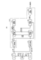
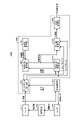
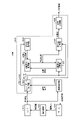
- FIG. 1 is a diagram showing a configuration example of an information processing system 100 including an information processing device 1000 according to the first embodiment.
- the information processing system 100 includes an information processing device 1000, a mechanical device 1008, a sensor 1010, a motor 1009, and a device control unit 1099.
- the motor 1009 drives the mechanical device 1008 by applying a driving force to the mechanical device 1008.
- the sensor 1010 measures the physical quantity of the mechanical device 1008. Examples of physical quantities measured by the mechanical device 1008 are position, velocity, acceleration, operation command, current, voltage, torque, force, pressure, voice, or light quantity.
- the motor speed and the motor torque will be described as an example.
- the motor speed is the rotation speed of the motor 1009
- the motor torque is the torque generated by the motor 1009.
- the sensor 1010 outputs a sensor signal including a measured value of a physical quantity to the information processing device 1000 and the device control unit 1099.
- the device control unit 1099 determines a control signal for controlling the motor 1009 based on the sensor signal.
- the motor 1009 is controlled by a control signal output from the device control unit 1099.
- the information processing device 1000 includes a sensor data acquisition unit 1001, an internal variable holding unit 1002, an internal variable calculation unit 1003, a feature quantity calculation unit 1004, an initialization processing unit 1005, and a state diagnosis unit 1006.
- the sensor data acquisition unit 1001 acquires the measured value of the physical quantity of the mechanical device 1008 measured by the sensor 1010. As described above, the measured value of the physical quantity is included in the sensor signal transmitted by the sensor 1010. Further, the sensor data acquisition unit 1001 holds the measured values from the first time point to the Nth time point among the acquired measured values as sensor data.
- N is an integer of 2 or more.
- the internal variable holding unit 1002 temporarily holds a smaller number of internal variables than N. Internal variables are variables that are sequentially calculated in time series based on sensor data. Internal variables are used to calculate features. Details of internal variables and features will be described later.
- the internal variable calculation unit 1003 receives the sensor data transmitted from the sensor data acquisition unit 1001 and the internal variables transmitted from the internal variable holding unit 1002.
- the internal variable calculation unit 1003 updates the internal variable based on the sensor data and the internal variable. More generalized, the internal variable calculation unit 1003 calculates the internal variable corresponding to the j + 1th time point based on the sensor data at the j + 1th time point and the internal variable corresponding to the jth time point, so that the internal variable can be calculated. Will be updated sequentially.
- j is an integer from 1 to N-1. That is, the internal variable calculation unit 1003 calculates the internal variable at a certain time point based on the sensor data at a certain time point and the internal variable one time point before the certain time point.
- the calculated internal variable is transmitted to the internal variable holding unit 1002.
- the feature amount calculation unit 1004 receives the sensor data transmitted from the sensor data acquisition unit 1001 and the internal variables transmitted from the internal variable holding unit 1002. The feature amount calculation unit 1004 calculates the feature amount based on the sensor data and the internal variables. More generally, the feature amount calculation unit 1004 calculates the feature amount obtained by extracting the statistical features included in the sensor data from the first time point to the Nth time point based on the internal variables. The calculated feature amount is transmitted to the state diagnosis unit 1006.
- the initialization processing unit 1005 executes the initialization processing.
- the initialization process is a process of setting an internal variable held by the internal variable holding unit 1002 to an initial value. More generally, the initialization processing unit 1005 performs a process of determining the internal variable at the first time point to a value between the preset maximum value and the preset minimum value.
- the state diagnosis unit 1006 performs a diagnostic process for diagnosing the state of the mechanical device 1008 based on the feature amount, and outputs a diagnostic result which is the result of the diagnostic process.
- FIG. 2 is a diagram showing a hardware configuration example of the mechanical device 1008 and its peripheral device according to the first embodiment.
- FIG. 2 shows a mechanical device 1008 using a servomotor 1230 as a drive source as a configuration example of the mechanical device 1008.
- the drive torque generated by the servo motor 1230 is output from the servo motor shaft 1231 and input to the ball screw shaft 1224 via the coupling 1220.
- the ball screw 1210 converts the rotational movement into a linear movement by a screw mechanism, and operates the movable portion 1212.
- the movable portion 1212 is connected to different mechanical parts, and the moved mechanical parts are used according to the purpose of the mechanical device 1008.
- the movable portion 1212 is restricted from moving in a desired direction by the guide 1213.
- the guide 1213 assists the movable portion 1212 so that the mechanical device 1008 can operate with high accuracy.
- the servomotor 1230 includes an encoder 1233 that measures the rotation angle and a current sensor 1232 that measures the current so that the servomotor shaft 1231 can be driven following a predetermined position, speed, or torque. It is common that and is attached.
- the driver 1240 performs feedback control based on the information obtained from the current sensor 1232, and supplies the electric power required for driving to the servomotor 1230. The calculation required for feedback control is performed by the device control unit 1099 in FIG.
- the motor torque is exemplified as an example of the sensor data used for diagnosing the state, but the present invention is not limited to this. Any physical quantity such as position, velocity, acceleration, current, voltage, torque, force, pressure, voice, and light amount described above may be used as long as the state of the mechanical device 1008 is included as information. Further, instead of these physical quantities, image information or the like may be used.
- the current sensor 1232 and the encoder 1233 are illustrated, but the present invention is not limited thereto.
- a laser displacement sensor, a gyro sensor, a vibrometer, an acceleration sensor, a voltmeter, a torque sensor, a pressure sensor, a microphone, an optical sensor, a camera and the like can be exemplified.
- the mounting position of the sensor 1010 does not necessarily have to be close to the servomotor 1230, and may be a position suitable for diagnosing the state of the mechanical device 1008.
- an acceleration sensor may be installed on the outer surface of the guide 1213 or the like, and the acceleration may be measured as sensor data.
- the PLC (Programmable Logic Controller) 1260 sends an operation command of the servomotor 1230 to the driver 1240.
- a PC Personal Computer
- PC1270 may be prepared as needed.
- PC1270 is used to send a command to PLC1260.
- an industrial PC Fractory Automation PC or Industrial PC
- a PLC display 1250 for monitoring the status of the PLC 1260 and a PC display 1280 for monitoring the status of the PC 1270 may be prepared.
- a plurality of drive sources such as the servomotor 1230 are provided in one mechanical device 1008. Therefore, a plurality of drivers 1240 may be prepared as needed.
- a single PLC1260 may control or a plurality of PLC1260s may cooperate to operate the mechanical device 1008. Also in the case of these configurations, the information processing apparatus 1000 shown in the present embodiment can be implemented in the same manner.
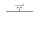
- FIG. 3 is a diagram showing a configuration example in the case where the processing circuit included in the driver 1240 shown in FIG. 2 is configured by the processor 1291 and the memory 1292.
- the processing circuit is composed of a processor 1291 and a memory 1292
- each function of the processing circuit of the driver 1240 is realized by software, firmware, or a combination of software and firmware.
- the software or firmware is written as a program and stored in memory 1292.
- each function is realized by the processor 1291 reading and executing the program stored in the memory 1292. That is, the processing circuit includes a memory 1292 for storing a program in which the processing of the driver 1240 will be executed as a result. It can also be said that these programs cause the computer to execute the procedures and methods of the driver 1240.
- the processor 1291 may be a computing means called a CPU (Central Processing Unit), a processing device, a computing device, a microprocessor, a microcomputer, or a DSP (Digital Signal Processor).
- the memory 1292 may be, for example, a non-volatile or volatile semiconductor memory such as a RAM, a ROM (Read Only Memory), a flash memory, an EPROM (Erasable Project ROM), or an EEPROM (registered trademark) (Electrically EPROM). Further, the memory 1292 may be used as a storage means such as a magnetic disk, a flexible disk, an optical disk, a compact disk, a mini disk, or a DVD (Digital Versaille Disc).
- FIG. 4 is a diagram showing a configuration example in the case where the processing circuit included in the driver 1240 shown in FIG. 2 is configured with dedicated hardware.
- the processing circuit 1293 shown in FIG. 4 may be, for example, a single circuit, a composite circuit, a programmed processor, a parallel programmed processor, an ASIC (Application Specific Integrated Circuit), or the like. FPGA (Field Processor Metal Gate Array) or a combination thereof may be used.
- the functions of the driver 1240 may be realized by the processing circuit 1293 for each function, or a plurality of functions may be collectively realized by the processing circuit 1293.
- the driver 1240 and the PLC1260 may be connected via a network. Further, the PC1270 may exist on the cloud server.
- An example of the hardware configuration is as described above, but the driver 1240, PLC1260, and PC1270 are not indispensable, and a device for implementing the information processing device according to the present disclosure is separately prepared and implemented inside the device. May be good.
- a single device having a battery, a microcomputer, a sensor, a display, and a communication function may be used, and the state of the mechanical device 1008 may be estimated based on the sensor data obtained by acquiring the sound of the mechanical device 1008 with a microphone. good.
- the indicators are not essential, and instead of displaying the results on the PLC display 1250 or the PC display 1280, the driver 1240, the existing LED provided in the PLC 1260, etc. are used to display the results. It may be displayed. Further, the servomotor 1230 may be stopped driving when it is diagnosed that an abnormality has occurred without showing the result on the display.
- the motor speed is obtained from the encoder 1233 provided in the servomotor 1230, but the present invention is not limited to this.
- the motor speed may be obtained by using a control signal from the device control unit 1099 that gives a drive command to the motor 1009.
- the servo motor 1230 has been described as a rotary servo motor, but other motors or drive sources such as linear servo motors, inducer motors, stepping motors, brush motors, ultrasonic motors, etc. May be carried out using.
- the ball screw 1210 and the coupling 1220 are examples of components and are not limited thereto.
- the information processing device according to the present disclosure can also be applied to a mechanical device composed of various other parts such as a speed reducer, a guide, a belt, a screw, a pump, a bearing, and a housing.
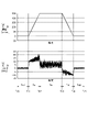
- FIG. 5 is a diagram showing time-series waveforms of the motor speed and the motor torque in the first embodiment.
- the signal directly obtained from the current sensor 1232 is a signal obtained by measuring the three-phase current flowing in the motor 1009.
- the motor torque can be calculated by applying appropriate conversion to the three-phase current.
- the three-phase current values detected by the current sensor 1232 may be used for diagnosis as sensor data.
- the signal obtained from the encoder 1233 is position information representing the rotation angle of the motor 1009. Therefore, if the position information is subjected to processing such as numerical differentiation, the motor speed, which is the rotation speed of the motor 1009, can be obtained. Therefore, instead of the signal obtained from the current sensor 1232, the signal obtained from the encoder 1233 may be used for diagnosis as sensor data.
- FIGS. 5 (a) and 5 (b) represents time.
- FIG. 5A shows a time-series waveform of the motor speed
- FIG. 5B shows a time-series waveform of the motor torque. These are the waveforms when a single drive called positioning is performed from the state where the motor 1009 is stopped.
- the sampling cycle which is the acquisition cycle of the waveform in FIG. 5B, is 0.5 milliseconds
- the sampling period, acquisition time, and data score N shown here are examples, and are not limited to these numerical values.
- the number of positionings is one, but the number of positionings may be a plurality of times. Further, although the operation when positioning the motor 1009 will be described here, the present invention is not limited to this. This embodiment can also be applied to controls other than positioning, such as speed control or torque control.
- the motor speed of FIG. 5A will be described.
- the motor 1009 is stopped between the time Tr0 and the time Tr1, and the motor speed is 0 [r / min]. This period is referred to as "Ts1”.
- the motor 1009 accelerates between the time Tr1 and the time Tr2, and the motor speed increases to 500 [r / min]. This period is referred to as "Ta”.
- the motor speed is constant and remains at 500 [r / min]. This period is referred to as "Te”.
- the motor 1009 decelerates between the time Tr3 and the time Tr4, and the motor speed decreases to 0 [r / min].
- the motor torque shown in FIG. 5 (b) will be described.
- the motor 1009 is stopped, and the motor torque required for the operation of the motor 1009 is almost 0 [Nm].
- a torque for accelerating the mechanical device 1008 is required, and a motor torque larger than the period Ts1 is generated. If viscous friction is present in the mechanical device 1008 due to the influence of viscous friction or the like, the required torque may gradually increase depending on the speed, as shown in FIG. In the following period Te, the speed of the mechanical device 1008 does not change, and a substantially constant motor torque is generated.
- the motor torque described above is the torque required for the operation of the almost ideal mechanical device 1008.
- a large or small noise as shown in FIG. 5B is generated in the motor torque.
- the ball screw shaft 1224, guide 1213, coupling 1220, etc. which are parts of the mechanical device 1008, deteriorate, the magnitude of the above-mentioned friction or vibration changes, and the influence of friction or vibration appears on the sensor data including the motor torque. It is known. Therefore, the sensor data is analyzed by a statistical method, and some indexes called feature quantities are calculated to detect the abnormality of the device.
- the sensor data acquisition unit 1001 acquires sensor signals sequentially generated from the sensor 1010 in time series and generates digitized sensor data.
- the generated sensor data is passed to at least one of the internal variable calculation unit 1003 and the feature quantity calculation unit 1004.
- the sensor data acquisition unit 1001 may execute a filter process for removing noise irrelevant to the state of the mechanical device 1008, if necessary.
- the functions and operations of the internal variable holding unit 1002, the internal variable calculation unit 1003, the feature amount calculation unit 1004, and the initialization processing unit 1005 will be described in detail by taking some types of feature amounts as examples.
- the time when the acquisition of the sensor data used for the feature amount calculation is started is called the "first time point".
- a total of N sensor data can be obtained from the first time point to the Nth time point.
- N is an integer of 2 or more.
- the time point at which the jth sensor data is acquired is referred to as "the jth time point”.
- j is an integer from 1 to N-1.
- the sensor data obtained at the j-th time point is referred to as "x j ".
- the sensor data will be acquired at predetermined time intervals. Needless to say, the sensor data may be acquired irregularly.
- the internal variable holding unit 1002 holds the internal variables one time before.
- the number of internal variables is not limited to one, and a plurality of types may be retained depending on the feature amount. The smaller the type of internal variable to be retained is smaller than the number of time series of sensor data on which the feature amount is calculated, the higher the memory reduction effect is.
- the internal variable holding unit 1002 may hold the feature amount itself as one kind of internal variable.
- the initialization processing unit 1005 executes the initialization processing for setting the retained internal variables to the initial values.
- the initial value is a value set at the time of initialization processing.
- the initialization processing unit 1005 performs the initialization processing at the first time point when the power of the information processing apparatus 1000 is turned on and the sensor data acquisition unit 1001 first acquires the sensor data.
- the initial value is easily set to 0 as described later, but it does not necessarily have to be 0.
- an upper limit value and a lower limit value may be set in the vicinity of an appropriate initial value, and the initial value may be appropriately determined between the upper limit value and the lower limit value.
- the calculation may not be stable if the internal variables and the initial values of the features are set to extremely small values.
- the calculation is stabilized by setting the initial value to a value other than 0.
- features whose steady-state values for sensor data are not zero.
- the convergence of the calculation can be accelerated by setting the value of the assumed feature amount as the initial value.
- the kurtosis which is one of the feature quantities shown in the present embodiment, has a value of about 3 with respect to the sensor data having a property close to a normal distribution. Therefore, by setting the initial value of kurtosis to 3, it is possible to perform calculations with quick convergence for many types of sensors.
- the average value mj for the sensor data x1 to xj from the first time point to the jth time point is defined by the following known mathematical formula (1).
- This formula (1) is also called an arithmetic mean value or an arithmetic mean value.
- the sensor data at the i -th time point is xj. Therefore, the average value m 3 at the third time point can be expressed by the following mathematical formula (2).
- the time-series sensor data from the first time point to the third time point is not stored in the memory 1292, and the information of the third time point is held as some internal variables. Then, consider a method of obtaining the average value of the fourth time point based on the internal variables of the third time point and the sensor data of the fourth time point.
- the average value m 4 at the fourth time point can be expressed as the following mathematical formula (3) according to the mathematical formula (1) which is the definition formula.
- the sensor data of the time series from the first to the fourth time point is used, and a memory for holding the sensor data for the number of past samples is required. It becomes.
- the average value m j + 1 at the time of the j + 1 can be expressed by the following mathematical formula (5).
- the average value m j + 1 at the time point j + 1 is sequentially obtained by the following mathematical formula (6).
- variable L j + 1 at the time point j + 1 is sequentially obtained by the following mathematical formula (7).
- Holding the variable at the jth time point in the above formula (7) is equivalent to holding the information of the time j during the sequential calculation.
- the sensor data x j + 1 is newly acquired at the time point j + 1.
- the internal variables to be held at the j-th time point in order to obtain the mean value m j + 1 at the j + 1th time point are the mean value m j and the variable L j .
- the variance v j for the sensor data x 1 to x j from the first time point to the jth time point is defined by the following known mathematical formula (8).
- an unbiased variance with a denominator of j-1 may be used, but in that case as well, it can be derived by the same procedure.
- the variance v j + 1 for the sensor data x1 to xj + 1 from the first time point to the j + 1st time point can be expressed by the following mathematical formula (11).
- the variance v j + 1 can be expressed by the following mathematical formula (12).
- the variable L j + 1 at the time point j + 1 is sequentially obtained by the above-mentioned mathematical formula (7). Further, the average value m j + 1 at the time point j + 1 is sequentially obtained by the above-mentioned mathematical formula (6). Then, the sensor data x j + 1 at the time j + 1 is newly acquired at the time j + 1.
- the internal variables to be held at the j-th time point in order to obtain the variance v j + 1 at the j + 1th time point are the variable L j , the variance v j , and the mean value m j .
- the standard deviation s j may be held instead of the variance v j .
- the initial values L 1 and v 1 of the variables L and the variance v should be set to 0 for the sake of simplicity, or the sensor during the initialization process should be used to avoid fluctuations immediately after the initialization process. It is better to decide according to the value of the data. However, if the initial value v 1 of the variance v is set to a value close to 0, the calculation is not stable when the variance v appears in the denominator in the sequential calculation of another feature amount described later. Therefore, it may be good to use a value larger than 0 as the initial value.
- the standard deviation s j with respect to the sensor data x 1 to x j from the first time point to the jth time point is defined by the following known mathematical formula (15).
- the standard deviation s j is immediately obtained from the variance v j sequentially obtained by the above procedure. Therefore, the internal variables to be retained for sequentially calculating the standard deviation s j are the same as the variance v j .
- the root mean square rj for the sensor data x1 to xj from the first time point to the jth time point is defined by the following known mathematical formula (16). This is also called RMS (Root Mean Square: effective value).
- the root mean square r j + 1 for the sensor data from the first time point to the j + 1st time point can be expressed by the following mathematical formula (17).
- variable L j + 1 at the time point j + 1 is sequentially obtained by the above-mentioned mathematical formula (7). Further, the sensor data x j + 1 at the time j + 1 is newly acquired at the time j + 1. As a result, the internal variables to be held at the j-th time point to obtain the root mean square square root r j 2 at the j + 1th time point are the root mean square square root square r j 2 and the variable L j .
- the calculation procedure for the sequential calculation of the skewness w is shown.
- the sensor data x is regarded as a random variable and the mean value m and the standard deviation s of the random variable x are used, the skewness w is defined by the following known mathematical formula (20).
- the modification of the above formula (21) utilizes the property that the expected value E [x] of the sensor data x is equal to the average value m.
- variable Aj at the jth time point can be expressed by the following mathematical formula (23).
- variable A j + 1 at the time point j + 1 can be expressed by the following mathematical formula (24).
- variable A j + 1 can be expressed as the following formula (25).
- variable A j + 1 at the time point j + 1 is sequentially obtained by the following formula (26).
- variable L j + 1 at the time point j + 1 is sequentially obtained by the above-mentioned mathematical formula (7). Further, the sensor data x j + 1 at the time j + 1 is newly acquired at the time j + 1.
- the internal variables to be held at the j-th time point in order to obtain the variable A j + 1 at the j + 1-th time point are the variable A j and the variable L j .
- variable B j at the time j can be expressed by the following mathematical formula (27).
- the skewness w j + 1 with respect to the sensor data x j + 1 from the first time point to the j + 1st time point can be obtained by the following mathematical formula (29).
- variable A j + 1 at the time point j + 1 is sequentially obtained by the above-mentioned mathematical formula (26). Further, the average value m j + 1 at the time point j + 1 is sequentially obtained by the above-mentioned mathematical formula (6). Then, the root mean square r j 2 at the time point j + 1 is sequentially obtained by the above-mentioned mathematical formula (19). Further, the standard deviation s j + 1 at the time point j + 1 is sequentially obtained by the above-mentioned mathematical formula (15). Then, the sensor data x j + 1 at the time j + 1 is newly acquired at the time j + 1.
- the internal variables to be held at the jth time point are the variables A j , Lj, the mean value m j , and the root mean square.
- the root mean square r j 2 and the standard deviation s j are the variables A j , Lj, the mean value m j , and the root mean square.
- the root mean square r j 2 and the standard deviation s j are the variables A j , Lj, the mean value m j , and the root mean square.
- the root mean square r j 2 and the standard deviation s j are the variance v j may be retained instead of the standard deviation s j .
- the root mean square r j may be held instead of the root mean square r j 2 .
- the initial values of the variables A j , Lj, the mean value m j , the root mean square square r j 2 , and the standard deviation s j are set to 0. Or, in order to avoid fluctuation immediately after the initialization process, it is better to determine according to the value of the sensor data at the time of the initialization process.
- the kurtosis k is defined by the following known mathematical formula (30).
- E [] represents the expected value of the random variable in square brackets.
- the kurtosis for a random variable having a normal distribution is 3.
- the modification of the above formula (31) utilizes the property that the expected value E [x] of the sensor data x is equal to the average value m.
- the expected value E [x 4 ] of the first numerator on the right side is represented by the variable C j .
- the expected value of the second term and the expected value of the third term of the molecule on the right side can be expressed by variables A j and B j , respectively. Therefore, the kurtosis k j can be expressed by the following mathematical formula (32).
- the standard deviation s j , the variables A j , and B j can be sequentially calculated by the above formulas (15), formula (26), and formula (27), respectively.
- variable Cj at the time j can be expressed by the following mathematical formula (33).
- variable C j + 1 at the time point j + 1 can be expressed by the following mathematical formula (34).
- variable C j + 1 can be expressed as the following formula (35).
- the variable B j agrees with the above-mentioned root mean square square square r j 2 . Therefore, the kurtosis k j for the sensor data x 1 to x j from the first time point to the jth time point can be obtained by the following mathematical formula (37).
- the kurtosis k j + 1 for the sensor data x 1 to x j + 1 from the first time point to the j + 1st time point can be obtained by the following mathematical formula (38).
- variable C j + 1 at the time point j + 1 is sequentially obtained by the above-mentioned mathematical formula (36). Further, the variable A j + 1 at the time point j + 1 is sequentially obtained by the above-mentioned mathematical formula (26). Then, the average value m j + 1 at the time point j + 1 is sequentially obtained by the above-mentioned mathematical formula (6). Further, the root mean square square r j 2 at the time point j + 1 is sequentially obtained by the above-mentioned mathematical formula (19). Further, the standard deviation s j + 1 at the time point j + 1 is sequentially obtained by the above-mentioned mathematical formula (15).
- the sensor data x j + 1 at the time j + 1 is newly acquired at the time j + 1.
- the internal variables to be held at the jth time point are the variables A j , L j , C j , and the mean value m. j , the root mean square squared r j 2 , and the standard deviation s j .
- the variance v j may be retained instead of the standard deviation s j .
- the root mean square r j may be held instead of the root mean square r j 2 .
- the initial values of the variables A j , L j , C j , the mean value m j , the root mean square square r j 2 , and the standard deviation s j It is better to set to 0 or to determine according to the value of the sensor data at the time of the initialization processing in order to avoid the fluctuation immediately after the initialization processing. Further, it is known that the kurtosis has a value of about 3 when it is known that the sensor data has a property close to a normal distribution. Therefore, the initial value k 1 of the kurtosis k may be set to 3.
- the maximum value aj for the sensor data x1 to xj from the first time point to the jth time point is defined by the following known mathematical formula (39).
- the sequential calculation method of the maximum value a can be easily realized by the following method.
- the maximum value a j at the jth time point is retained, and the larger of the sensor data xj at the j + 1th time point and the maximum value aj at the jth time point is held as the maximum value aj + 1 at the j + 1th time point. .. That is, the maximum value a j + 1 at the time point j + 1 can be sequentially calculated by the following mathematical formula (40).
- the minimum value n j for the sensor data x 1 to x j from the first time point to the jth time point is defined by the following known mathematical formula (41).
- the sequential calculation method of the minimum value n can be easily realized by the following method.
- the minimum value n j at the jth time point is retained, and the smaller of the sensor data xj at the j + 1th time point and the minimum value nj at the jth time point is held as the minimum value nj + 1 at the j + 1th time point. .. That is, the minimum value n j + 1 at the time point j + 1 can be sequentially calculated by the following mathematical formula (42).
- the peak value pj from the first time point to the jth time point is defined by the following formula (43).
- the peak value is the largest absolute value among the sensor data x1 to xj .
- the sequential calculation method of the peak value can be realized by the following method.
- the peak value p j at the jth time point is retained, and the larger of the sensor data x j at the j + 1th time point and the peak value pj at the jth time point is held as the peak value pj + 1 at the j + 1th time point. That is, the peak value p j + 1 at the time point j + 1 can be sequentially calculated by the following mathematical formula (44).
- the peak value is obtained by the following formula (45). You can also.
- the peak value can be obtained by the following mathematical formula (46).
- the internal variable to be held at the jth point in order to obtain the peak value pj + 1 at the j + 1th time point is the peak value pj .
- the maximum value a j and the minimum value n j may be held instead of the peak value p j .
- Peak The peak value is the difference between the maximum value and the minimum value. It is also called peak-to-peak.
- the peak peak value pp j for the sensor data x1 to xj from the first time point to the jth time point is defined by the following known mathematical formula (47).
- the peak peak value pp j can be immediately obtained by sequentially calculating the maximum value a j and the minimum value n j from the above-mentioned mathematical formulas (40) and (42).
- the peak peak value pp j + 1 can be obtained by the following known mathematical formula (48).
- the internal variables to be held at the jth time point in order to obtain the peak peak value pp j + 1 at the j + 1th time point are the maximum value a j and the minimum value n j .
- the wave height rate pr j with respect to the sensor data x1 to xj from the first time point to the jth time point is defined by the following mathematical formula (49).
- the peak factor pr j is a value obtained by dividing the above-mentioned peak value p j by the above-mentioned root mean square r j .
- the crest factor pr j is sometimes referred to as peak to RMS (peak-to-RMS) or crest factor. If it is known that the sensor data has a value biased in the positive direction, the maximum value a j may be used instead of the peak value p j .
- the wave height rate pr j + 1 for the sensor data x1 to xj from the first time point to the j + 1st time point can be obtained by the following mathematical formula (50).
- the peak value pj + 1 is sequentially calculated using the above-mentioned formula (44) or formula (45), and the root mean square r j + 1 is sequentially calculated using the formula (19).
- the wave height rate pr j + 1 can be obtained immediately.
- the internal variables to be held at the jth time point are the peak value pj and the root mean square square r j2 .
- the maximum value a j and the minimum value n j may be held instead of the peak value p j .
- the root mean square r j 2 of the root mean square instead of the root mean square r j may be retained.
- the internal variable calculation unit 1003 sequentially calculates the internal variables for calculating each feature amount.
- the feature amount calculation unit 1004 can determine the feature amount corresponding to the sensor data x1 to xj from the first time point to the Nth time point.
- the updated formula and the internal variables held by the internal variable holding unit 1002 are different for each type of feature amount.
- the feature amount is that the internal variable holding unit 1002 holds the internal variable, the internal variable calculation unit 1003 sequentially calculates the internal variable, and the feature amount calculation unit 1004 calculates the feature amount based on the internal variable. It is the same regardless of the type of.
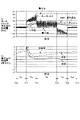
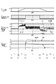
- FIG. 6 is a diagram showing time-series waveforms of the motor torque and various feature quantities in the first embodiment.
- the notation of the symbol attached to the feature amount and the like will be omitted as appropriate.
- FIG. 6 (a) shows the same motor torque waveform as that shown in FIG. 5 (b).
- the horizontal axis of FIGS. 6A and 6B represents time.
- FIG. 6A shows a time series of mean value, standard deviation, root mean square (RMS), maximum value and minimum value having the same unit [Nm] as the motor torque among the dimensional features.
- the waveform is shown.
- the peak value is the difference between the maximum value and the minimum value, and is not shown for simplicity. Further, the peak value is a value indicating a value having a large absolute value among the maximum value and the minimum value, and is not shown for simplicity.
- the variance is the square of the standard deviation and is not shown because the units are different.
- FIG. 6B shows a time-series waveform of skewness, kurtosis, and crest factor, which are dimensionless features, that is, features having no unit.
- the average value was almost 0 in the period Ts1, gradually increased in the period Ta, slightly decreased in the period Te, gradually decreased in the period Td, and slightly decreased in the period Ts2.
- the standard deviation is a small value that is almost constant in the period Ts1, gradually increases in the period Ta, slightly decreases in the period Te, gradually increases in the period Td, and slightly decreases in the period Ts2.
- the root mean square is a small value that is almost constant in the period Ts1, gradually increases in the period Ta, decreases slightly in the period Te, is almost constant in the period Td, and decreases slightly in the period Ts2.
- the maximum value is a small positive value that is almost constant in the period Ts1, increases every time the motor torque exceeds the past maximum value in the period Ta, and is constant in the period Te, the period Td, and the period Ts2.
- the minimum value is a small negative value that is almost constant in the period Ts1, constant in the period Ta and Te, decreases every time the motor torque exceeds the past minimum value in the period Td, and is constant in the period Ts2. ..
- the skewness is almost 0 in the period Ts1, increases sharply to a large positive value at the time Tr1 at which the period Ta starts, gradually decreases to a small value in the subsequent period Ta, and increases slightly in the period Te. It decreased slightly in the period Td and increased slightly in the period Ts2.
- the kurtosis increases from about 2 to about 3 in the period Ts1, increases sharply to a large positive value at the time Tr1 when the period Ta starts, gradually decreases to a small value in the subsequent period Ta, and slightly in the period Te. In the period Td, it increased slightly and then decreased, and in the period Ts2, it increased slightly.
- the wave height rate increases from about 2 to about 3 in the period Ts1, increases sharply to a large positive value at the time Tr1 when the period Ta starts, gradually decreases to a small value in the subsequent period Ta, and slightly in the period Te. In the period Td, it is almost constant, and in the period Ts2, it increases slightly.
- the feature amount at each time point shown in FIGS. 6A and 6B is a sequential calculation of the feature amount with respect to the motor torque in the past from each time point. Therefore, for example, the average value is a value obtained by batch calculation while holding the motor torque for the entire period (Ts1 + Ta + Te + Td + Ts2) in FIG. 6 (a), and a time Tr5 which is the final time in FIG. 6 (a) sequentially obtained. Matches the value of.
- the feature amount calculation unit 1004 in order to make the transition of the feature amount easy to change, the feature amount calculation unit 1004 also calculates each feature amount for each sensor data acquisition cycle.
- the internal variable calculation unit 1003 needs to sequentially calculate the internal variable for each acquisition cycle of the sensor data.
- the feature amount calculation unit 1004 is necessary. The feature amount may be calculated accordingly.
- the feature amount calculation unit 1004 may be configured to calculate the feature amount only once at the time point Tr5, that is, when the data score N of the sensor data reaches 12000. With this configuration, it is possible to reduce the computational load of the information processing apparatus 1000.
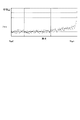
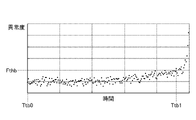
- FIG. 7 is a diagram showing an example of the secular variation of the feature amount in the first embodiment.
- FIG. 7 shows the results of periodically plotting the features calculated by the above method. Regular means, for example, monthly.
- the horizontal axis of FIG. 7 is time, which represents the operating time of the mechanical device 1008.
- the state diagnosis unit 1006 sets a threshold value Fth1 for the feature amount, and when the feature amount exceeds the threshold value Fth1, diagnoses that an abnormality has occurred in the mechanical device 1008.
- the feature amount any of the above-mentioned feature amounts may be used. Further, a plurality of feature quantities may be calculated and individual threshold values may be set for each feature quantity.
- the time Tta0 is the time when the operation is started.
- the feature amount from the time Tta0 to the time before the time Tta1 keeps a value smaller than the threshold value Fth1 although there is some variation.
- the state diagnosis unit 1006 makes a diagnosis that the mechanical device 1008 is normal, and outputs the diagnosis result.
- the state diagnosis unit 1006 makes a diagnosis that an abnormality has occurred in the mechanical device 1008 at the time Tta1, and outputs the diagnosis result.
- the threshold value Fth1 may be determined based on the feature amount when an abnormality occurs in another mechanical device in the past. Further, the threshold value Fth1 may be determined with reference to the feature amount immediately after the operation of the mechanical device 1008 is started. Further, the threshold value Fth1 may be set dynamically. For example, while operating a plurality of mechanical devices 1008, the feature amounts thereof may be calculated individually, and the threshold value Fth1 may be changed periodically in consideration of the variation in the feature amounts for each device. Further, the threshold value Fth1 may be determined based on the feature amount obtained by a simulation or the like in consideration of the characteristics of the mechanical device 1008.
- the threshold value Fth1 represents the upper limit value of the normal state, but when a feature amount in which a smaller value indicates an abnormality is used, the lower limit value of the normal state is used as the threshold value. It may be set as Fth1. Further, two threshold values consisting of an upper limit value and a lower limit value may be used in combination. Further, the diagnosis result does not have to be one, and the diagnosis may be performed for a plurality of feature quantities and the diagnosis result may be output for each feature quantity.
- the method is not limited to this method.
- a statistical method such as performing a test based on the distribution of the degree of abnormality for a certain period may be adopted.
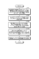
- FIG. 8 is a flowchart provided for explaining the information processing method according to the first embodiment.
- the sensor data acquisition unit 1001 acquires the measured value of the physical quantity as sensor data from the sensor 1010 that measures the physical quantity of the mechanical device 1008 at each time point from the first time point to the Nth time point (N is an integer of 2 or more).
- the internal variable holding unit 1002 holds a number of internal variables smaller than N, which are sequentially calculated based on the sensor data (step S102).
- the internal variable calculation unit 1003 calculates the internal variable corresponding to the j + 1th time point (j is an integer from 1 to N-1) based on the sensor data at the j + 1st time point and the internal variable corresponding to the jth time point. (Step S103).
- the feature amount calculation unit 1004 calculates the feature amount obtained by extracting the statistical features included in the sensor data from the first time point to the Nth time point based on the internal variables of the Nth time point (step S104).
- the state diagnosis unit 1006 diagnoses the state of the mechanical device based on the feature amount (step S105).
- a step of executing an initialization process for determining an internal variable at a first time point to a value between a preset maximum value and a minimum value may be included.
- the sensor data acquisition unit acquires the measured value of the physical quantity of the mechanical device measured by the sensor, and starts from the first time point among the measured values.
- the measured values up to the Nth time point (N is an integer of 2 or more) are retained as sensor data.
- the internal variable holding unit holds a number of internal variables smaller than N, which are sequentially calculated in time series based on the sensor data.
- the internal variable calculation unit calculates the internal variable corresponding to the j + 1th time point (j is an integer from 1 to N-1) based on the sensor data at the j + 1st time point and the internal variable corresponding to the jth time point.
- the feature amount calculation unit calculates the feature amount obtained by extracting the statistical features included in the sensor data from the first time point to the Nth time point based on the internal variables of the Nth time point. According to the information processing apparatus configured as described above, it is not necessary to hold the sensor data from the first time point to the Nth time point by holding the number of internal variables smaller than N. As a result, it is possible to obtain an unprecedented remarkable effect that the feature amount can be calculated without using a computer having a high computing power and a computer having a large storage capacity.
- the information processing device includes a state diagnosis unit that diagnoses the state of the mechanical device based on the feature amount.
- a state diagnosis unit that diagnoses the state of the mechanical device based on the feature amount.
- the information processing apparatus includes an initialization processing unit that executes an initialization process for determining an internal variable at a first time point to a value between a preset maximum value and a preset minimum value. May be.
- the physical quantity at each time point from the first time point to the Nth time point (N is an integer of 2 or more) from the sensor for measuring the physical quantity of the mechanical device.
- the measured value of is acquired as sensor data.
- a smaller number of internal variables than N which are sequentially calculated in time series based on the sensor data, are held.
- the internal variable corresponding to the j + 1th time point (j is an integer from 1 to N-1) is calculated based on the sensor data at the j + 1st time point and the internal variable corresponding to the jth time point.
- the feature amount obtained by extracting the statistical features included in the sensor data from the first time point to the Nth time point is calculated based on the internal variables of the Nth time point.
- the state of the mechanical device is diagnosed based on the feature amount. According to the information processing method including the processes of the first to fifth steps, a smaller number of internal variables than N are held, so that it is necessary to hold the sensor data from the first time point to the Nth time point. There is no. As a result, it is possible to obtain an unprecedented remarkable effect that information processing for diagnosing the state of a mechanical device can be performed without using a computer having a high computing power and a computer having a large storage capacity.
- the internal variable at the first time point is initially determined to be a value between a preset maximum value and a preset minimum value. It may include a step to execute the conversion process. By including such an initialization processing step, the probability of erroneous determination can be reduced and the accuracy of the diagnostic processing can be improved.
- FIG. 9 is a diagram showing a configuration example of the information processing system 100A including the information processing apparatus 2000 according to the second embodiment.
- the information processing device 1000 is replaced with the information processing device 2000
- the device control unit 1099 is replaced with the device control unit 2099.
- the sensor data acquisition unit 1001 is replaced by the sensor data acquisition unit 2001
- the internal variable calculation unit 1003 is replaced by the internal variable calculation unit 2003
- the feature quantity calculation unit 1004 is replaced by the feature quantity calculation unit 2004. It has been replaced.
- Other configurations are the same as or equivalent to the information processing system 100 shown in FIG.
- the same or equivalent components are designated by the same reference numerals, and duplicate description will be omitted.
- the sensor data acquisition unit 2001 In addition to the processing of the sensor data acquisition unit 1001, the sensor data acquisition unit 2001 generates a calculation permission flag for determining whether or not to update the internal variable based on the operation signal. More generally, the sensor data acquisition unit 2001 has at least one of an acquisition cycle, which is an interval of time for acquiring sensor data, an operation signal indicating the operation status of the mechanical device 1008, and a data value in the sensor data. Two or more time points between the first time point and the jth time point (j is an integer from 1 to N-1 (where N is an integer of 2 or more)) are determined based on the above, and two or more points are determined. Generates a compute permission flag to update internal variables based on the time point in.
- the internal variable calculation unit 2003 updates the internal variable when the calculation permission flag contains the content of updating the internal variable, in addition to the processing of the internal variable calculation unit 1003. On the other hand, when the calculation permission flag does not include the content to update the internal variable, the internal variable calculation unit 2003 performs a process of inheriting the value of the internal variable from the previous time. More generally, the internal variable calculation unit 2003 uses the internal variable calculation unit 2003 to indicate each u-th time point indicated by the calculation permission flag (u is an integer of 1 or more and j or less (where j is an integer from 1 to N-1 and N). Is an integer of 2 or more)), the internal variable at the u + 1 time point is determined to be the value of the internal variable at the uth time point.
- the feature amount calculation unit 2004 updates the feature amount when the calculation permission flag includes the content to update the feature amount, in addition to the processing of the feature amount calculation unit 1004. If the calculation permission flag does not include the content to update the feature amount, the feature amount calculation unit 2004 performs a process of inheriting the feature amount from the previous time.
- the device control unit 2099 outside the information processing device 2000 outputs an operation signal indicating the operation status of the mechanical device 1008 in addition to the processing of the device control unit 1099.
- the mechanical device 1008 is, for example, a mechanical device driven by a motor
- sensor data with less noise can be obtained when the feature amount when the speed is constant is used, and the state of the mechanical device 1008 can be estimated with high accuracy. be. Therefore, by configuring the internal variables and the values of the feature amount to be updated only when the speed of the motor 1009 is constant, it becomes possible to calculate the feature amount more useful for the state diagnosis of the mechanical device 1008. ..
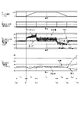
- FIG. 10 is a diagram showing time-series waveforms of motor torque and various feature quantities in the second embodiment.
- FIG. 10 (a) shows the same waveform as the time-series waveform of the motor speed shown in FIG. 5 (a). Further, FIG. 10B shows a time-series waveform of the calculation permission flag determined by the sensor data acquisition unit 2001.
- the flag value is set to "1" when the internal variable is updated, and the flag value is set to "0" when the internal variable is not updated.
- the sensor data acquisition unit 2001 sets the flag value of the calculation permission flag to "1” in the period Te from the time Tr2 to the time Tr3 so that the internal variable is updated when the speed is not "0" and is constant. It is supposed to be. Further, in a period other than the period Te, that is, in the period Ts1, the period Ta, the period Td, and the period Ts2, the sensor data acquisition unit 2001 sets the flag value of the calculation permission flag to “0”. In FIG. 9, an example of constant speed is set to 500 [r / min].
- the internal variable is not updated when the speed is 0 is that the mechanical device 1008 does not operate when the motor 1009 is stopped, and the information corresponding to the state of the mechanical device 1008 does not appear in the sensor data. Can be mentioned. However, depending on the configuration of the mechanical device 1008, information according to the state of the mechanical device 1008 may appear in the sensor data even when the motor 1009 is stopped. In such a case, the internal variables may be configured to be updated even when the system is stopped. The operation when the flag value of the calculation permission flag is "0" does not have to change the internal variables and the feature amount. For example, even if the calculation is performed so that the current value is overwritten with the previous value. The calculation itself may be skipped.
- the speed and acceleration of the motor are used as operation signals.
- the flag value of the calculation permission flag is set to "1".
- the reference acceleration and speed may be determined in advance with reference to the specifications of the mechanical device 1008 or the motor 1009.
- the operation signal is obtained from the device control unit 2099.
- the flag value of the calculation permission flag is set to "1" when the predetermined time is reached after the motor 1009 starts to move, and the flag value of the calculation permission flag is set to "0" after another predetermined time has elapsed. You may try to do it.
- the sampling cycle which is the time interval for acquiring the sensor data.
- FIG. 10 (c) shows a time-series waveform of the motor torque similar to that shown in FIG. 5 (b). Further, FIG. 10 (c) shows a time-series waveform having the same feature amount as that shown in FIG. 6 (a). Further, FIG. 10 (d) shows a time-series waveform having the same feature amount as that shown in FIG. 6 (b).
- the values of the feature amounts in FIGS. 10 (c) and 10 (d) did not change in the period Ts1, the period Ta, the period Td, and the period Ts2 excluding the period Te.
- the internal variable calculation unit 2003 and the feature amount calculation unit 2004 are configured so that the internal variables and the feature amount are not updated during the period other than the period Te. Because it is.
- the period Te all the features are updated at any time, and by the time Tr3, which is the end point of the period Te, the features have converged to almost constant values. According to such a configuration, in addition to the effect of the first embodiment, the state of the mechanical device 1008 can be estimated with higher accuracy.
- the sensor data acquisition unit has an acquisition cycle which is an interval of time for acquiring sensor data, an operation signal indicating the operation status of the mechanical device, and a sensor. Two or more time points between the first time point and the jth time point are determined based on at least one of the data values in the data, and the calculation permission flag is generated based on the determined two or more point points.
- the internal variable calculation unit determines the internal variable at the u + 1 time point as the value of the internal variable at the uth time point for each uth time point (u is an integer of 1 or more and j or less) indicated by the calculation permission flag. According to the information processing device configured in this way, sensor data with less noise can be obtained according to the operating state of the mechanical device. As a result, after obtaining the effect of the first embodiment, the effect that the state of the mechanical device can be estimated with high accuracy can be obtained.
- FIG. 11 is a diagram showing a configuration example of the information processing system 100B including the information processing apparatus 3000 according to the third embodiment.
- the information processing apparatus 2000 is replaced with the information processing apparatus 3000 in the configuration of the information processing system 100A shown in FIG.
- the sensor data acquisition unit 2001 is replaced by the sensor data acquisition unit 3001
- the initialization processing unit 1005 is replaced by the initialization processing unit 3005.
- Other configurations are the same as or equivalent to the information processing system 100A shown in FIG.
- the same or equivalent components are designated by the same reference numerals, and duplicate description will be omitted.
- the sensor data acquisition unit 3001 In addition to the processing of the sensor data acquisition unit 1001 shown in FIG. 1, the sensor data acquisition unit 3001 generates an initialization trigger for determining a time point for initializing an internal variable. More generalized and more specifically, the sensor data acquisition unit 3001 has a acquisition cycle which is an interval of time for acquiring sensor data, an operation signal indicating the operation status of the mechanical device 1008, and sensor data. Determine one or more time points between the first and Nth time points based on at least one, and generate an initialization trigger to initialize the internal variables based on the determined one or more time points. ..
- the initialization processing unit 3005 performs the initialization processing of the internal variables based on the time point indicated by the initialization trigger in addition to the processing of the initialization processing unit 1005.
- the tendency of the feature amount may differ depending on the operating conditions such as acceleration, rotation at a constant speed, deceleration, and stop. In such a case, it may be possible to estimate the state of the mechanical device 1008 with high accuracy by separating the calculation of the feature amount for each operating condition. Therefore, by initializing the internal variables at the time when the operating condition changes, such as when the speed change of the motor 1009 is changed, it becomes possible to calculate the feature amount which is more useful for estimating the state of the mechanical device 1008.
- FIG. 12 is a diagram showing time-series waveforms of the motor torque and various feature quantities in the third embodiment.
- FIG. 12 (a) shows the same waveform as the time-series waveform of the motor speed shown in FIG. 5 (a). Further, FIG. 12B shows a time-series waveform of the initialization trigger determined by the sensor data acquisition unit 3001.
- the signal level is set to "1" when the internal variable is initialized, and the signal level is set to "0" when the internal variable is not initialized.
- the sensor data acquisition unit 3001 sets the signal level of the initialization trigger at time Tr1, time Tr2, time Tr3 and time Tr4 to "1" so as to initialize the internal variable when the motor speed changes, that is, when acceleration occurs.
- the signal level is set to "0" at other times.
- the jerk of the motor that is, the time derivative of the acceleration is used as the operation signal.
- the signal level of the initialization trigger is set to "1".
- the reference jerk size should be determined in advance with reference to the specifications of the mechanical device 1008 or the motor 1009.
- the operation signal is obtained from the device control unit 2099.
- the signal level of the initialization trigger may be momentarily set to "1" when the predetermined time is reached after the motor 1009 starts to move.
- the signal level of the initialization trigger may be momentarily set to "1" every time a specific time elapses.
- the sampling cycle which is the time interval for acquiring the sensor data.
- the initialization trigger may be determined so that the initialization process is performed when the motor 1009 starts to move.
- FIG. 12 (c) shows a time-series waveform of the motor torque similar to that shown in FIG. 5 (b). Further, FIG. 12 (c) shows a time-series waveform having the same feature amount as that shown in FIG. 6 (a). Further, FIG. 12 (d) shows a time-series waveform having the same feature amount as that shown in FIG. 6 (b).
- each feature quantity of FIGS. 10 (c) and 10 (d) begins to change immediately after the time Tr0, the time Tr1, the time Tr2, the time Tr3 and the time Tr4, and each period Ts1, period Ta, period Te, and period By the end of Td and the period Ts2, each feature quantity has converged to a substantially constant value.
- the state of the mechanical device 1008 can be estimated with higher accuracy.
- it can be applied to the case where the motor 1009 is operated under the condition that the motor 1009 does not have a constant speed, so that the applicable range can be expanded.
- the sensor data acquisition unit has an acquisition cycle which is an interval of time for acquiring sensor data, an operation signal indicating the operation status of the mechanical device, and a sensor.
- an acquisition cycle which is an interval of time for acquiring sensor data, an operation signal indicating the operation status of the mechanical device, and a sensor.
- the initialization processing unit executes a process of initializing an internal variable based on an initialization trigger. According to the information processing apparatus configured in this way, it is possible to separate the calculation of the feature amount for each operating condition.
- the effect of the first embodiment it is possible to further obtain the effect that the state of the mechanical device can be estimated with high accuracy. Further, since it can be applied to the case where the motor is operated under the condition that the motor does not have a constant speed, the effect that the application range regarding the operating condition can be further expanded after obtaining the effect of the second embodiment can be obtained.
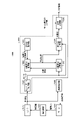
- FIG. 13 is a diagram showing a configuration example of the information processing system 100C including the information processing apparatus 4000 according to the fourth embodiment.
- the information processing apparatus 3000 is replaced with the information processing apparatus 4000 in the configuration of the information processing system 100B shown in FIG.
- the internal variable calculation unit 1003 is replaced with the internal variable calculation unit 4003
- the feature amount calculation unit 1004 is replaced with the feature amount calculation unit 4004
- the state diagnosis unit 1006 is replaced with the state diagnosis unit 4006.
- a convergence degree calculation unit 4007 is newly provided.
- Other configurations are the same as or equivalent to the information processing system 100B shown in FIG.
- the same or equivalent components are designated by the same reference numerals, and duplicate description will be omitted.
- the internal variable calculation unit 4003 calculates the internal variable based on the oblivion coefficient in addition to the processing of the internal variable calculation unit 1003.
- the feature amount calculation unit 4004 also calculates the feature amount based on the forgetting coefficient in addition to the processing of the feature amount calculation unit 1004.
- the forgetting coefficient is a coefficient for weighting the feature amount so that the effect of the sensor data with the new time on the feature amount is larger than the effect of the sensor data with the old time on the feature amount. It has a small value.
- the convergence degree calculation unit 4007 calculates the degree of convergence, which is an index that quantitatively indicates the degree of convergence in the calculation of the feature amount, based on the internal variables.
- the state diagnosis unit 4006 diagnoses the state of the mechanical device 1008 based on the feature amount at the time when the convergence degree calculated by the convergence degree calculation unit 4007 satisfies a certain condition.
- the calculation procedure for the sequential calculation of the exponential moving average is shown.
- a weighted average value considering the weight given for each time is known.
- the weighted average value there is a method of averaging the weighted sensor data weighted by multiplying the forgetting coefficient ⁇ .
- the forgetting coefficient ⁇ is a coefficient for weighting the time so that the effect of the time on the new sensor data is greater than the effect of the time on the old sensor data.
- this process is referred to as an exponential moving average, and the value is referred to as an exponential moving average value.
- the exponential moving average is sometimes referred to as the exponential smoothing moving average.
- "1- ⁇ " obtained by subtracting the forgetting coefficient ⁇ from "1" may be referred to as a smoothing coefficient.
- the exponential moving average value m'j for the sensor data x1 to xj from the first time point to the jth time point is defined by the following mathematical formula (51).
- the exponential moving average value m'3 at the third time point can be expressed by the following mathematical formula (52).
- the coefficient in the latest data is larger than that in the old data as described above (0.81 ⁇ 0.9 ⁇ 1). It can be said that the recent data, that is, the new data of the time, is emphasized when calculating the average.
- the exponential moving average value m'j + 1 with respect to the sensor data x1 to xj + 1 from the first time point to the j + 1st time point can be transformed by the following mathematical formula (53).
- the exponential moving average value m'j + 1 at the time point j + 1 is sequentially obtained by the following mathematical formula (54).
- the sensor data x j + 1 is newly acquired at the time point j + 1. Further, the variable L' j at the time of the j + 1 can be expressed by the following mathematical formula (55).
- variable L' j + 1 at the time of the j + 1 can be expressed by the following mathematical formula (56).
- variable L'j + 1 at the time point j + 1 can be sequentially calculated by the following mathematical formula (57).
- the internal variables that should be retained for calculating the exponential moving average m'j + 1 at the j + 1th time point are the exponential moving average value m'j and the variable L' j at the jth time point.
- the forgetting coefficient ⁇ is preferably set to a value larger than 0 and smaller than 1.
- the forgetting coefficient ⁇ is close to 1, it is difficult to forget the past information, and when it is close to 0, it is easy to forget the past information.
- the forgetting coefficient ⁇ is set to 1, the information of the sensor data is not forgotten, and the formula of the sequential calculation is the same as that of the first embodiment. Further, when the forgetting coefficient is set to 0, the information of all the sensor data is forgotten when one time elapses, so that the feature amount for the sensor data of the past two or earlier cannot be obtained.
- the forgetting factor should be set to a value close to 1 and less than 1, for example, 0.9 to 0.999.
- the time constant ⁇ can be calculated by the following mathematical formula (58).
- the oblivion coefficient ⁇ may be set by using the estimated frequency (unit rad / s) which is the reciprocal of the time constant ⁇ .
- the calculation procedure for the sequential calculation of the exponential movement variance is shown.
- the variance using the weighted sensor data weighted by multiplying the forgetting coefficient ⁇ for each time is called “exponential movement variance”.
- the exponential movement variance v'j + 1 for the sensor data x1 to xj + 1 from the first time point to the j + 1st time point can be expressed by the following mathematical formula (60).
- variable L'j + 1 at the time point j + 1 is sequentially obtained by the above-mentioned mathematical formula (57). Further, the exponential moving average value m'j + 1 at the time point j + 1 is sequentially obtained by the above-mentioned mathematical formula (54). Then, the sensor data x j + 1 at the time j + 1 is newly acquired at the time j + 1.
- the internal variables to be held at the j-th time point in order to obtain the exponential moving variance v'j + 1 at the j + 1th time point are the variable L' j , the exponential moving variance v'j , and the exponential moving average value m'j .
- the exponential movement standard deviation s'j described later may be retained.
- the initial values L' 1 , v'1, m'1 of the variables L', exponential moving variance v'and exponential moving average m' are set to 0 .
- the exponential movement standard deviation s'j with respect to the sensor data x1 to xj from the first time point to the jth time point is defined by the following formula (64) from the exponential movement variance v'j .
- the exponential movement standard deviation s'j is immediately obtained from the exponential movement variance v'j sequentially obtained by the above procedure. Therefore, the internal variable to be retained for sequentially calculating the exponential movement standard deviation s'j is the same as the exponential movement variance v'j .
- the calculation procedure for the sequential calculation of the exponentially moving root mean square is shown.
- the root mean square using the weighted sensor data weighted by multiplying the forgetting coefficient ⁇ for each time is called an "exponentially moving root mean square".
- the exponential movement root mean square r'j for the sensor data x1 to xj from the first time point to the jth time point is defined by the following mathematical formula (65).
- the exponential root mean square r'j + 1 for the sensor data x1 to xj + 1 from the first time point to the j + 1st time point can be expressed by the following mathematical formula (66).
- variable L'j + 1 at the time point j + 1 is sequentially obtained by the above-mentioned mathematical formula (57). Further, the sensor data x j + 1 is newly acquired at the time point j + 1. As a result, the internal variables to be held at point j in order to obtain the square root of the exponentially moved root mean square at the j + 1 point are the square r'j 2 of the exponentially moved root mean square and the variable L' j . be.
- the calculation procedure for the sequential calculation of the exponential movement skewness is shown.
- the skewness using the weighted sensor data weighted by multiplying the forgetting coefficient ⁇ for each time is called "exponential skewness”.
- the exponential movement skewness w'j for the sensor data x1 to xj from the first time point to the jth time point is the following formula (69). Can be expressed by.
- the exponential moving average value m'j of the above formula (69) can be sequentially calculated by the above formula (54), and the exponential moving standard deviation s'j of the above formula (69) can be calculated sequentially by the above formula (54). It can be calculated sequentially in (63) and (64).
- variables A'j and B'j at the jth time point can be expressed by the following mathematical formulas (70) and (71).
- variable A'j + 1 at the time of the j + 1 can be expressed by the following mathematical formula (72).
- variable A'j + 1 can be expressed as the following formula (73).
- variable A'j + 1 at the time j + 1 is sequentially obtained by the following formula (74).
- the internal variables to be held at the jth time point in order to obtain the variable at the j + 1th time point are the variables L' j and A'j .
- the variable L'j + 1 at the time point j + 1 is sequentially obtained by the above-mentioned mathematical formula (57).
- the variable B'j at the jth time point can be expressed by the following mathematical formula (75).
- variable B'j matches the square root r'j 2 of the exponential moving square root mean square as in the above formula (75), which is sequential in the above formula (68). Is required. Therefore, the exponential movement skewness w'j for the sensor data x1 to xj from the first time point to the jth time point can be obtained by the following mathematical formula (76).
- the exponential movement skewness w'j + 1 with respect to the sensor data x1 to xj + 1 from the first time point to the j + 1st time point can be obtained by the following mathematical formula (77).
- variable A'j + 1 at the time point j + 1 is sequentially obtained by the above-mentioned mathematical formula (74). Further, the exponential moving average value m'j + 1 at the time point j + 1 is sequentially obtained by the above-mentioned mathematical formula (54). Then, the square root r'j 2 of the exponential moving square root mean square at the j + 1st time point is sequentially obtained by the above-mentioned mathematical formula (68). Further, the exponential movement standard deviation s'j + 1 at the time point j + 1 is sequentially obtained by the above-mentioned mathematical formula (64). Then, the sensor data x j + 1 at the time j + 1 is newly acquired at the time j + 1.
- the internal variables to be held at the jth time point are the variables A'j, L' j , and the exponent.
- the exponential movement variance v'j may be retained instead of the exponential movement standard deviation s'j .
- the exponential moving square root mean square r'j may be held instead of the square root r'j 2 of the exponentially moving root mean square.
- the calculation procedure for the sequential calculation of the exponential movement kurtosis is shown.
- the kurtosis using the weighted sensor data weighted by multiplying the forgetting coefficient ⁇ for each time is called "exponential kurtosis”.
- the exponential movement kurtosis k'j for the sensor data x1 to xj from the first time point to the jth time point is the following formula (78). Can be expressed by.
- variable C'j at the jth time point can be expressed by the following mathematical formula (79).
- variable C'j + 1 at the time of the j + 1 can be expressed by the following mathematical formula (80).
- variable C'j + 1 can be expressed as the following formula (81).
- the variable B'j matches the square root r'j 2 of the exponentially moving root mean square, and the square r'j 2 of the exponentially moved root mean square is described above. It is sequentially obtained by the formula (68) of. Therefore, the exponential movement kurtosis k'j for the sensor data x1 to xj from the first time point to the jth time point can be obtained by the following mathematical formula (83).
- the exponential movement kurtosis k'j + 1 with respect to the sensor data x1 to xj + 1 from the first time point to the j + 1st time point can be obtained by the following mathematical formula (84).
- variable C'j + 1 at the time point j + 1 is sequentially obtained by the above-mentioned mathematical formula (82). Further, the variable A'j + 1 at the time point j + 1 is sequentially obtained by the above-mentioned mathematical formula (74). Then, the exponential moving average value m'j + 1 at the time point j + 1 is sequentially obtained by the above-mentioned mathematical formula (54). Further, the square root r'j + 1 2 of the exponential moving square root mean square at the j + 1st time point is sequentially obtained by the above-mentioned mathematical formula (68).
- the exponential movement standard deviation s'j + 1 at the time point j + 1 is sequentially obtained by the above-mentioned mathematical formulas (63) and (64). Then, the sensor data x j + 1 at the time j + 1 is newly acquired at the time j + 1. As a result, the square r'j 2 of the first time point or the exponential moving square root mean square is sequentially obtained by the above formula (68).
- the internal variables to be held at the jth time point are the variables A'j, L' j , and the exponential movement average value m'j .
- Exponential movement square root mean square r'j 2 Exponential movement square root mean square r'j 2 and exponential movement standard deviation s'j .
- the exponential movement variance v'j may be retained instead of the exponential movement standard deviation s'j .
- the exponential moving square root mean square r'j may be held instead of the square root r'j 2 of the exponentially moving root mean square.
- the exponential movement kurtosis k'j has a value of about 3 when it is known that the sensor data has a property close to a normal distribution. Therefore, the initial value k ' 1 of the exponential movement kurtosis k'j may be set to 3.
- the calculation of the maximum value, the minimum value, the peak peak value, the peak value, and the peak rate (hereinafter, appropriately referred to as "maximum value, etc.") in which the latest time is weighted is as shown in the first embodiment. It is not possible to update the current maximum value, etc. from the previous maximum value, etc. However, for example, some candidate values that are likely to be the maximum value may be retained as internal variables, and the retained candidate values may be deleted after the specified time has elapsed. By doing so, it is possible to calculate the maximum value or the like corresponding to the sensor data of the latest time.
- the degree of convergence that quantitatively represents the degree of convergence of the sequential calculation can be calculated from the internal variables.
- the variable L' j which is one of the internal variables, is sequentially calculated by the mathematical formula (57), it asymptotically approaches the value of 1 / (1- ⁇ ) regardless of the input sensor data. You can see that. Therefore, when the initial value L' 1 of the variable L' j is 0 or more and less than 1 / (1- ⁇ ), the following formula (85) can be used so that the degree of convergence can be a value from 0 to 1. It is conceivable to define the degree of convergence di with.
- the degree of convergence is calculated using the above formula (85), but the degree of convergence is not limited to the above, and any definition can be used as long as the value increases with the convergence of the calculation. good. However, the value increases monotonically as the calculation converges, and the one that asymptotics to a specific value is easy to use as a reference.
- ⁇ (1- ⁇ ) L' j ⁇ M which is obtained by multiplying the entire right side of the above formula (85) by the Mth power (M is a positive real number), is defined as the degree of convergence.
- This degree of convergence is a preferable definition expression because it takes a value from 0 to 1 and increases monotonically with the convergence of the calculation.
- FIG. 14 is a diagram showing time-series waveforms of motor torque and various feature quantities in the fourth embodiment.
- FIG. 14 (a) shows the same waveform as the time-series waveform of the motor speed shown in FIG. 5 (a). Further, FIG. 14 (b) shows the same waveform as the time-series waveform of the initialization trigger shown in FIG. 12 (b).
- FIG. 14C shows a time-series waveform of the degree of convergence calculated by the degree of convergence calculation unit 4007 using the mathematical formula (85).
- the degree of convergence is 0 at the time Tr0 when the sequential calculation starts, the time Tr1, the time Tr2, the time Tr3, and the time Tr4 where the initialization trigger indicates “1”. This is because the initialization process is executed and the variable L' j at the jth time point, which is one of the internal variables, becomes 0.
- the j-th time point indicates the time point when the initialization trigger indicates "1".
- the degree of convergence has increased since each initialization process was performed, and gradually approaches 1.
- FIG. 14 (d) shows a time-series waveform of the motor torque similar to that shown in FIG. 5 (b). Further, FIG. 14D shows a time-series waveform of the exponential moving average value, the exponential moving standard deviation, and the exponential moving square root mean square (RMS) having the same unit [Nm] as the motor torque. The notation of "exponential movement" is omitted to avoid complicating the figure.
- FIG. 14 (e) shows a time-series waveform of the exponential movement skewness and the exponential movement kurtosis, which are dimensionless features, that is, features having no unit.
- the forgetting coefficient ⁇ is 0.975.
- FIG. 14D the notation of “exponential movement” is omitted.
- the exponential moving average value follows the motor torque over the entire period from time Tr0 to time Tr5, although it is slightly behind the motor torque. This shows the nature of the present embodiment in which the average value is calculated by giving a large weight to the latest short-time motor torque.
- the exponential movement standard deviation is a small value that is almost constant during the period Ts1.
- period Ta period Te, period Td and period Ts2
- it increases immediately after the initialization trigger becomes 1, then decreases until the next initialization trigger becomes 1, and converges to an almost constant value. There is.
- the exponential moving root mean square is a small value that is almost constant during the period Ts1.
- Ta gradually increases with the increase of the motor torque.
- Te it converges to an almost constant value.
- Td it gradually increases as the absolute value of the motor 1009 increases.
- Ts2 it converges to a small value that is almost constant.
- the exponential movement skewness is almost 0 in the period Ts1. This is because the motor torque of the period Ts1 has a symmetrical probability distribution. At the time Tr1 at which the period Ta starts, the skewness temporarily becomes a positive value and then becomes a negative value. This is because the motor torque increases from 0, so that old data near 0 and new data after the increase are temporarily mixed, and the probability distribution of the motor torque is disturbed.
- the exponential movement skewness temporarily becomes a positive value immediately after the time Tr2 in the period Te, and then converges to almost 0.
- the exponential movement skewness temporarily becomes a positive value immediately after the time Tr3, and then converges to a substantially constant value.
- the exponential movement skewness temporarily becomes a negative value immediately after the time Tr4, and then converges to almost 0.
- the exponential movement kurtosis is about 3 in the period Ts1.
- the value of 3 is a characteristic of the exponential kurtosis with respect to the normal distribution, and indicates that the motor torque has a property close to the normal distribution in the period Ts1.
- the exponential movement kurtosis becomes a negative value immediately after the time Tr1 at which the period Ta starts, and becomes a positive value thereafter. After that, the exponential kurtosis has converged to a substantially constant value by time Tr2. This is because the motor torque increases from 0, so that old data near 0 and new data after the increase are temporarily mixed, and the probability distribution of the motor torque is disturbed.
- the exponential movement kurtosis becomes a negative value immediately after the time Tr2 at which the period Te starts, and then becomes a positive value. After that, the exponential kurtosis has converged to a substantially constant value by time Tr3.
- the exponential movement kurtosis becomes a negative value immediately after the time Tr3 at which the period Td starts, and then becomes a positive value. After that, the exponential kurtosis has converged to a substantially constant value by time Tr4.
- the exponential movement kurtosis becomes a negative value immediately after the time Tr4 at which the period Ts2 starts, and then becomes a positive value. After that, the exponential movement kurtosis is gradually converging to a constant value by the time Tr5.
- FIG. 15 is an enlarged view of the time-series waveform of the initialization trigger and the degree of convergence shown in FIG. 14 over a period from time Tr2 to time Tr3.
- the initialization trigger indicates “1”, and the initialization process is executed.
- the variable L' j at the jth time point which is one of the internal variables, becomes 0, and the degree of convergence becomes 0.
- the j-th time point indicates the time point when the initialization trigger indicates "1". The degree of convergence increases after initialization and gradually approaches 1.
- the state diagnosis unit 4006 diagnoses the state of the mechanical device 1008 based on the feature amount at the time when the convergence degree calculated by the convergence degree calculation unit 4007 using the mathematical formula (85) satisfies a certain condition.
- the threshold value Cth is set for the degree of convergence.
- the state diagnosis unit 4006 diagnoses the state of the mechanical device 1008 using the feature amount at the time when the degree of convergence exceeds the threshold value Cth.
- the threshold value Cth should be set to a value close to 1 in which the degree of convergence is asymptotic.
- An example of the threshold value Cth is 0.99.
- Tx the time when the threshold value Cth is exceeded.
- Tn the period from the time Tr2 to the time Tx in which the degree of convergence does not exceed the threshold value Cth
- Tc the period from the time Tx when the degree of convergence exceeds the threshold value Cth to Tr3
- the state diagnosis unit 4006 does not use the feature amount calculated in the period Tn for the diagnosis of the mechanical device 1008, but uses the feature amount calculated in the period Tc for the diagnosis of the mechanical device 1008. According to such a configuration, it is possible to use the feature amount when the calculation result is sufficiently converged when the internal variable is initialized. Thereby, in addition to the effect of the third embodiment, the state of the mechanical device can be estimated with higher accuracy.
- the information processing apparatus further includes a convergence degree calculation unit with respect to the configuration of the third embodiment.
- the convergence degree calculation unit calculates the degree of convergence, which is an index that quantitatively indicates the degree of convergence in the calculation of the feature quantity, based on the internal variables.
- FIG. 16 is a diagram showing a configuration example of the information processing system 100D including the information processing apparatus 5000 according to the fifth embodiment.
- the state diagnosis unit 1006 is replaced with the state diagnosis unit 5006.
- Other configurations are the same as or equivalent to the information processing system 100 shown in FIG.
- the same or equivalent components are designated by the same reference numerals, and duplicate description will be omitted.
- an example of applying the state diagnosis unit 5006 to the information processing apparatus 1000 shown in FIG. 1 will be described, but the information processing apparatus 2000, 3000, 4000 shown in FIGS. 9, 11 or 13 will be described. It may be applied to any of them.
- FIG. 17 is a diagram showing a configuration example of the state diagnosis unit 5006 in the fifth embodiment.
- the state diagnosis unit 5006 includes a state quantity acquisition unit 5401, a learning unit 5402, an abnormality degree calculation unit 5403, and a decision-making unit 5404.
- the state quantity acquisition unit 5401 acquires a state quantity including a feature quantity.
- the learning unit 5402 learns the relationship between the state of the mechanical device 1008 and the feature amount based on the state amount of the mechanical device 1008 in the normal state.
- the abnormality degree calculation unit 5403 calculates the abnormality degree, which is an index quantitatively indicating the abnormality degree of the mechanical device 1008, based on the learning result learned by the learning unit 5402.
- the decision-making unit 5404 determines the diagnosis result of diagnosing the state of the mechanical device 1008 based on the abnormality degree calculated by the abnormality degree calculation unit 5403.
- the state quantity acquisition unit 5401 acquires information including a set value given to the mechanical device 1008 as a state quantity together with the feature quantity.
- a set value given to the mechanical device 1008 As an example of the feature amount, it is conceivable to use the skewness calculated sequentially by the above method. Further, it is conceivable to use the set value of the motor speed as the information of the mechanical device 1008 used as one of the state quantities.
- the device control unit 1099 is set so that the maximum motor speed is 500 [r / min]. In the present embodiment, it is assumed that the set value of the motor speed is 500 [r / min].
- the input information to the state quantity acquisition unit 5401 is the set value of the skewness and the motor speed
- the input information to the state quantity acquisition unit 5401 may be 3 or more.
- FIG. 18 is a diagram showing the relationship between the feature amount and the set value of the motor speed in the fifth embodiment.
- a plurality of sets of the skewness which is an example of the feature amount, and the set value of the motor speed are plotted as one data.
- the horizontal axis is the set value of the motor speed, and the vertical axis is the skewness.
- the feature quantity may be plural, and the state quantity may be displayed by a three-dimensional concept. Further, a state quantity other than the motor speed may be used.
- the black circles are normal data in which the mechanical device 1008 is in a normal state.
- the white circles are abnormality data when some abnormality occurs in the mechanical device 1008. As shown in FIG.
- the mechanical device 1008 obtains a large number of state quantities in a normal state as normal data. Looking at FIG. 18, it can be seen that the normal data tends to have a larger feature amount as the set value of the motor speed is larger. On the other hand, the abnormal data has a relatively large feature amount even though the set value of the motor speed is relatively small.
- a method of calculating the abnormality degree using principal component analysis is known.
- Principal component analysis is a method of re-axising the state quantity, which is multidimensional data, in order from the direction of the largest variance.
- the learning unit 5402 using the principal component analysis calculates the eigenvalues and eigenvectors of the variance-covariance matrix of the normal data obtained in advance, and linearly maps the original state quantity to the space of the principal component. Assuming that the original state quantity is the vector x and the vector after mapping is y, the mapping of the vector x can be expressed by the following mathematical formula (86).
- the learning unit 5402 determines the expression matrix A, which is a matrix representing this linear map, based on the normal data.
- the learning unit 5402 obtains a plurality of eigenvalues and eigenvectors related to the variance-covariance matrix obtained from a plurality of prepared normal data. With respect to the obtained plurality of eigenvalues, a plurality of corresponding eigenvectors are arranged in descending order of the eigenvalues. Then, the matrix formed by the plurality of eigenvectors created side by side becomes the expression matrix A.
- an eigenvector of 2 rows and 1 column is created using two state quantities.
- two eigenvectors of 2 rows and 1 column are arranged side by side to create a 2 row and 2 column expression matrix.
- the dimension of the vector after mapping is made smaller than the dimension of the vector of the original state quantity. May be good.
- FIG. 19 is a diagram showing the results of principal component analysis in the fifth embodiment.
- the data of FIG. 18 is reprinted, and the axis of the first principal component having the largest eigenvalue and the axis of the second principal component having the second largest eigenvalue are shown.
- Eigenvalues are obtained as a result of principal component analysis.
- FIG. 19 in order to make the result of the principal component analysis easy to understand, according to the eigenvalues corresponding to the variance of each principal component, centering on the position where the axis of the first principal component and the axis of the second principal component intersect. , An elliptical confidence interval is shown.
- the confidence interval is the interval that is expected to fit in the distribution of the data with a certain probability. For example, there are 90% confidence intervals that are expected to fit 90% of normal data, 99% confidence intervals that are expected to fit 99% of normal data, and so on. Confidence intervals can be calculated using common statistical methods.
- the normal data is located inside the 99% confidence interval, while the abnormal data is located outside the 99% confidence interval. If the mechanical device 1008 is normal, this abnormal data is judged to be data that is considered to occur only with a probability of about 1%. Therefore, it is determined that there is a possibility that an abnormality has occurred in the mechanical device 1008. On the other hand, if a threshold value is simply set for the feature amount without using principal component analysis, the abnormal data may fall within the distribution of normal data, making diagnosis difficult.
- the abnormality degree calculation unit 5403 of the fifth embodiment calculates the abnormality degree which is an index which quantitatively indicates the degree of abnormality of the mechanical device 1008.
- An index called the T2 statistic is used as an example of the degree of anomaly.
- the T2 statistic is an index in which the data after mapping by principal component analysis standardizes the distance from the center coordinates of the axes of each principal component by the variance for each axis. The distance from the center coordinates of the axis of each principal component is also called "Mahalanobis distance".
- FIG. 20 is a diagram showing the degree of abnormality of the principal component analysis in the fifth embodiment.
- FIG. 20 shows a diagram when the normal data, the abnormal data, the 90% confidence interval, and the 99% confidence interval shown in FIG. 19 are standardized using the above-mentioned eigenvalues. Further, in FIG. 20, the distance between the point where the axis of the first principal component and the axis of the second principal component intersect and the abnormality data is shown as the degree of abnormality. Further, the 90% confidence interval and the 99% confidence interval, which were elliptical in FIG. 19, are circular in FIG. 20. As shown in FIG. 20, if the Mahalanobis distance is illustrated using the concept, it is possible to determine the degree of abnormality in consideration of the variation in the data at the normal time.
- the abnormality degree calculation unit 5403 described a method of calculating the abnormality degree by using the T2 statistic after mapping to the principal component obtained by the principal component analysis, but the present invention is not limited to this method.
- an index called the Q statistic may be used.
- unsupervised learning as a method that can learn normal data, remember its distribution, and calculate the degree of abnormality for new data in the same way as principal component analysis.
- a one-class support vector machine One class Support Vector Machine
- a Mahalanobis Taguchi Method a self-organizing map (Self-Organizing Maps), or the like
- the degree of abnormality may be calculated after performing preprocessing such as normalization processing on the input state quantity.
- the decision-making unit 5404 of the fifth embodiment determines the result of diagnosing the state of the mechanical device 1008 using the degree of abnormality calculated by the above method.
- a procedure for the decision-making unit 5404 to diagnose the state of the mechanical device 1008 using the feature amount will be described with reference to FIG.
- FIG. 21 is a diagram showing an example of the secular variation of the degree of abnormality in the fifth embodiment.
- FIG. 21 shows the result of periodically plotting the degree of anomaly calculated by the above method. Regular means, for example, monthly.
- the horizontal axis of FIG. 21 is time, which represents the operating time of the mechanical device 1008.
- the decision-making unit 5404 provides a threshold value Fthb for the degree of abnormality, and when the degree of abnormality exceeds the threshold value Fthb, it diagnoses that an abnormality has occurred in the mechanical device 1008.
- the time Ttb0 is the time when the operation is started.
- the degree of abnormality from the time Ttb0 to the time before the time Ttb1 keeps a value smaller than the threshold value Fthb, although there is some variation.
- the decision-making unit 5404 makes a diagnosis that the mechanical device 1008 is normal, and outputs the diagnosis result.
- the state diagnosis unit 5006 makes a diagnosis that an abnormality has occurred in the mechanical device 1008 at the time Ttb1, and outputs the diagnosis result.
- the threshold value Fthb there are various ways to determine the threshold value Fthb. For example, it is conceivable to set the threshold value Fthb as the degree of abnormality corresponding to the 99% confidence interval of normal data. Further, the degree of abnormality when an abnormality occurs in another mechanical device in the past may be set as the threshold value Fthb. Further, the degree of abnormality may be determined with reference to the degree of abnormality immediately after the operation of the mechanical device 1008 is started. Further, the threshold value Fthb may be set dynamically. For example, while operating a plurality of mechanical devices, the degree of abnormality may be calculated individually, and the threshold value Fthb may be determined periodically in consideration of the variation in the degree of abnormality for each device. When the information processing device is configured in this way, when one of the plurality of mechanical devices fails, the degree of abnormality of the failed device becomes larger than the degree of abnormality of the other devices, so that it is possible to detect the abnormality. Become.
- the method is not limited to this method.
- a statistical method such as performing a test based on the distribution of the degree of abnormality for a certain period may be adopted.
- the information processing apparatus diagnoses the state of the mechanical device based on the degree of abnormality, which is an index quantitatively indicating the degree of abnormality of the mechanical device. As a result, it is possible to obtain the effect of the other embodiments and to estimate the state of the mechanical device with high accuracy.
- FIG. 22 is a diagram showing a configuration example of the information processing system 100E including the information processing apparatus 6000 according to the sixth embodiment.
- the state diagnosis unit 1006 is replaced with the state diagnosis unit 6006 in the configuration of the information processing system 100 shown in FIG.
- Other configurations are the same as or equivalent to the information processing system 100 shown in FIG.
- the same or equivalent components are designated by the same reference numerals, and duplicate description will be omitted.
- an example of applying the state diagnosis unit 6006 to the information processing apparatus 1000 shown in FIG. 1 will be described, but the information processing apparatus 2000, 3000, 4000 shown in FIGS. 9, 11 or 13 will be described. It may be applied to any of them.
- FIG. 23 is a diagram showing a configuration example of the state diagnosis unit 6006 in the sixth embodiment.
- the state diagnosis unit 6006 includes a state quantity acquisition unit 6401, a learning unit 6402, a state estimation unit 6403, and a decision-making unit 6404.
- the state quantity acquisition unit 6401 acquires a state quantity including a feature quantity.
- the learning unit 6402 learns the relationship between the state of the mechanical device 1008 and the state amount based on the learning data that associates the state of the mechanical device 1008 with the state amount acquired by the state amount acquisition unit 6401.
- the state estimation unit 6403 estimates the state of the mechanical device 1008 based on the state amount input to the learning unit 6402 and the learning result by the learning unit 6402.
- the decision-making unit 6404 determines the diagnostic result of diagnosing the state of the mechanical device 1008 based on the result estimated by the state estimation unit 6403.
- the state quantity acquisition unit 6401 acquires information including a set value given to the mechanical device 1008 as a state quantity together with the feature quantity.
- a set value given to the mechanical device 1008 As an example of the feature amount, it is conceivable to use the skewness and kurtosis calculated sequentially by the above method. Further, it is conceivable to use the above-mentioned set value of the motor speed as the information of the mechanical device 1008 used as one of the state quantities.
- three cases where the input information to the state quantity acquisition unit 6401 is the set value of skewness, kurtosis, and motor speed are exemplified, but the present invention is not limited to this example.
- the input information to the state quantity acquisition unit 6401 may be 4 or more.
- the learning unit 6402 and the state estimation unit 6403 may learn the relationship between the state quantity and the state of the mechanical device 1008 by so-called supervised learning, for example, according to a neural network model.
- supervised learning by giving a large amount of learning data, which is a set of data of a certain input (state amount) and result (label), to the learning unit, a model that learns the features of those data and estimates the result from the input. Is called supervised learning.
- a neural network is composed of an input layer composed of a plurality of neurons, an intermediate layer (hidden layer) composed of a plurality of neurons, and an output layer composed of a plurality of neurons.
- the intermediate layer may be one layer or two or more layers.
- FIG. 24 is a diagram showing an example of the structure of the state estimation unit 6403 in the sixth embodiment.
- the input is a state quantity.
- the neural network of FIG. 24 has 3 inputs and 3 layers.
- the value obtained by multiplying the input value by the weight W1 composed of W11 to W16 is input to the intermediate layer composed of Y1 and Y2. Will be done.
- the value obtained by multiplying the input value of the intermediate layer by the weight W2 composed of W21 to W26 is output from the output layer composed of Z1 to Z3. This output result changes depending on the value of the weight W1 and the value of the weight W2.
- the state quantities 1 to 3 are input to the input layers X1 to X3, and the probability of each state output from the output layers Z1 to Z3 matches the label of the training data.
- the weights W1 and W2 are adjusted so as to do so.
- the information processing apparatus 6000 equipped with the learned state estimation unit 6403 that has executed the learning process in the sixth embodiment may be configured.
- the trained state estimation unit 6403 may be composed of trained data, trained programs, or a combination thereof. By using the learned state estimation unit 6403, the result of learning using another information processing device can be used, so that an information processing device 6000 capable of realizing diagnosis without performing new learning is provided. be able to.
- FIG. 24 shows an example in which the skewness is input to the input layer X1, the kurtosis is input to the input layer X2, and the set value of the motor speed is input to the input layer X3.
- the strain degree is an example of the state quantity 1 input to the input layer X1
- the sharpness is an example of the state quantity 2 input to the input layer X2
- the set value of the motor speed is input to the input layer X3.
- the probability that the ball screw shaft 1224 of the mechanical device 1008 has failed is output as the probability of the state 1.
- the probability that the coupling 1220 of the mechanical device 1008 has failed is output as the probability of the state 2.
- the probability that the mechanical device 1008 is in a normal state is output as the probability of the state 3.
- a softmax function softmax function
- this function makes the estimation result easier to understand.
- the neural network shown in FIG. 24 learns the relationship between the state of the mechanical device 1008 and the state quantities 1 to 3 by supervised learning according to a data set created based on the learning data input to the learning unit 6402. .
- the information indicating the true state of the mechanical device 1008 called the label is correctly obtained, and the output of any one of the states 1 to 3 is 1 (probability is 100%), and the other outputs are. It is better to learn so that it becomes 0 (probability is 0%).
- the configuration of the learning unit 6402 and the state estimation unit 6403 does not have to be limited to the neural network.
- there are many known methods such as k-nearest neighbor method, binary tree search, support vector machine, linear regression, logistic regression, etc., in which the relationship between the state quantity and the label is learned and the state is estimated from the state quantity. Therefore, the learning unit 6402 and the state estimation unit 6403 may be configured by applying this method.
- the decision-making unit 6404 determines the diagnosis result of diagnosing the state of the mechanical device 1008 based on the estimation result of the state estimation unit 6403. For example, when the mechanical device 1008 is most likely to be normal, it is preferable to output a diagnostic result indicating that the mechanical device 1008 is normal as a diagnostic result. Further, when the probability that the ball screw shaft 1224 has failed or the probability that the coupling 1220 has failed is the highest, it is preferable to output the diagnosis result indicating the failure location. Further, when the sum of the probability that the ball screw shaft 1224 has failed and the probability that the coupling 1220 has failed is larger than the normal probability, a result indicating that any part has failed is output. It is better to do it.
- the information processing apparatus learns the relationship between the state of the mechanical device and the state quantity based on the learning data that links the relationship between the state of the mechanical device and the state quantity.
- the state of the mechanical device is estimated based on the learning result and the state quantity used at the time of learning.
- the configuration shown in the above embodiments is an example, and can be combined with another known technique, can be combined with each other, and does not deviate from the gist. It is also possible to omit or change a part of the configuration.
- 100,100A, 100B, 100C, 100D, 100E Information processing system 1000,2000,3000,4000,5000,6000 Information processing device, 1001,2001,3001 Sensor data acquisition unit, 1002 Internal variable holding unit, 1003,2003 4003 Internal variable calculation unit, 1004, 2004, 4004 Feature quantity calculation unit, 1005, 3005 Initialization processing unit, 1006,400,500,6006 State diagnosis unit, 1008 mechanical device, 1009 motor, 1010 sensor, 1099, 2099 device control Part, 1210 ball screw, 1212 movable part, 1213 guide, 1220 coupling, 1224 ball screw shaft, 1230 servo motor, 1231 servo motor shaft, 1232 current sensor, 1233 encoder, 1240 driver, 1250, 1280 indicator, 1260 PLC, 1270 PC, 1291 processor, 1292 memory, 1293 processing circuit, 4007 convergence degree calculation unit, 5401, 6401 state quantity acquisition unit, 5402, 6402 learning unit, 5403 abnormality degree calculation unit, 6403 state estimation unit, 5404, 6404 decision unit ..
Landscapes
- Physics & Mathematics (AREA)
- Engineering & Computer Science (AREA)
- General Physics & Mathematics (AREA)
- Automation & Control Theory (AREA)
- Artificial Intelligence (AREA)
- Evolutionary Computation (AREA)
- Mathematical Physics (AREA)
- Chemical & Material Sciences (AREA)
- Combustion & Propulsion (AREA)
- Testing Of Devices, Machine Parts, Or Other Structures Thereof (AREA)
- Testing And Monitoring For Control Systems (AREA)
- Hardware Redundancy (AREA)
Abstract
Description
図1は、実施の形態1における情報処理装置1000を含む情報処理システム100の構成例を示す図である。情報処理システム100は、図1に示すように、情報処理装置1000と、機械装置1008と、センサ1010と、モータ1009と、装置制御部1099とを備える。モータ1009は、機械装置1008に駆動力を付与することで機械装置1008を駆動する。機械装置1008がモータ1009によって駆動される際、センサ1010は機械装置1008の物理量を計測する。機械装置1008が計測する物理量の例は、位置、速度、加速度、動作指令、電流、電圧、トルク、力、圧力、音声、又は光量である。なお、本実施の形態では、モータ速度及びモータトルクを一例として説明する。モータ速度はモータ1009の回転速度であり、モータトルクはモータ1009が発生するトルクである。











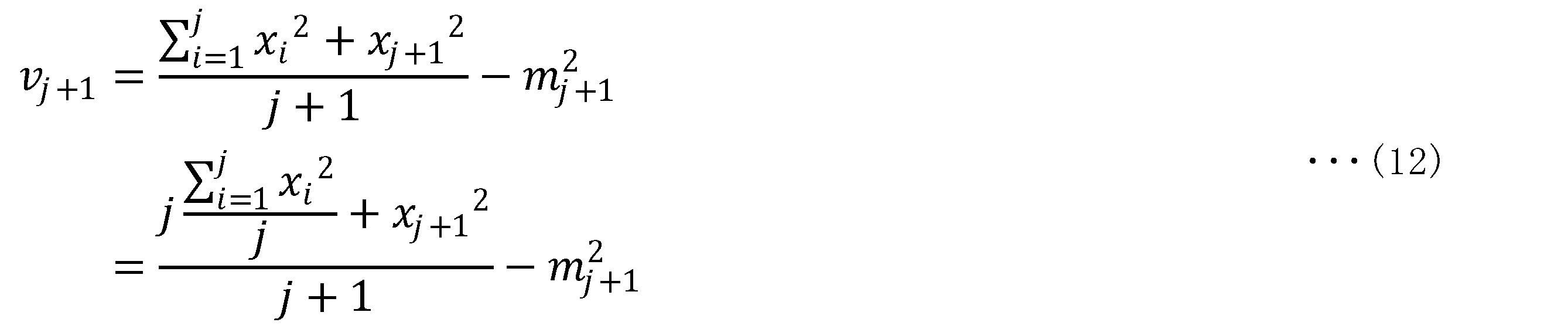










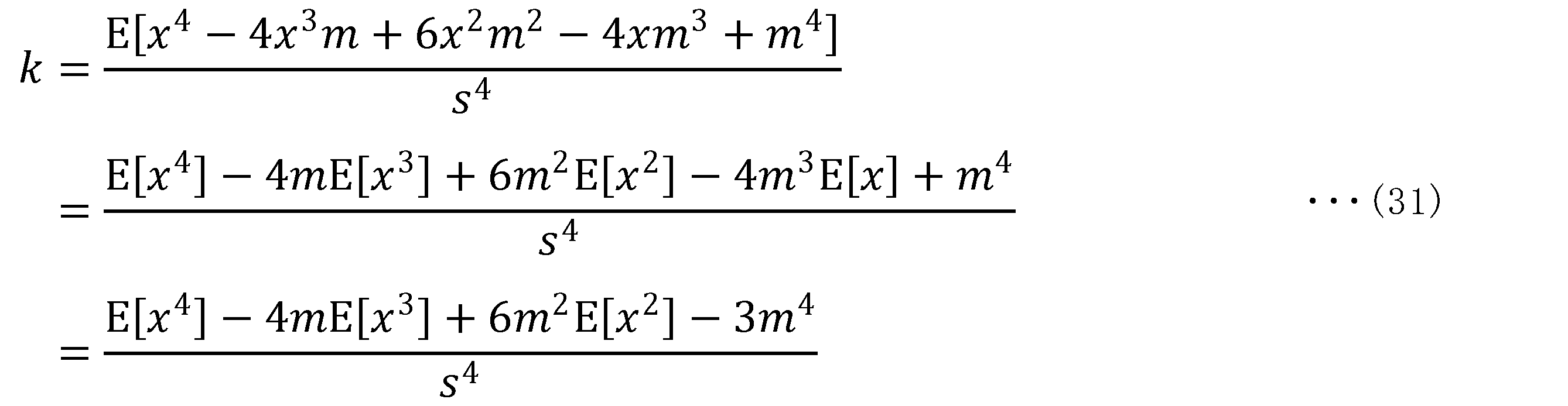



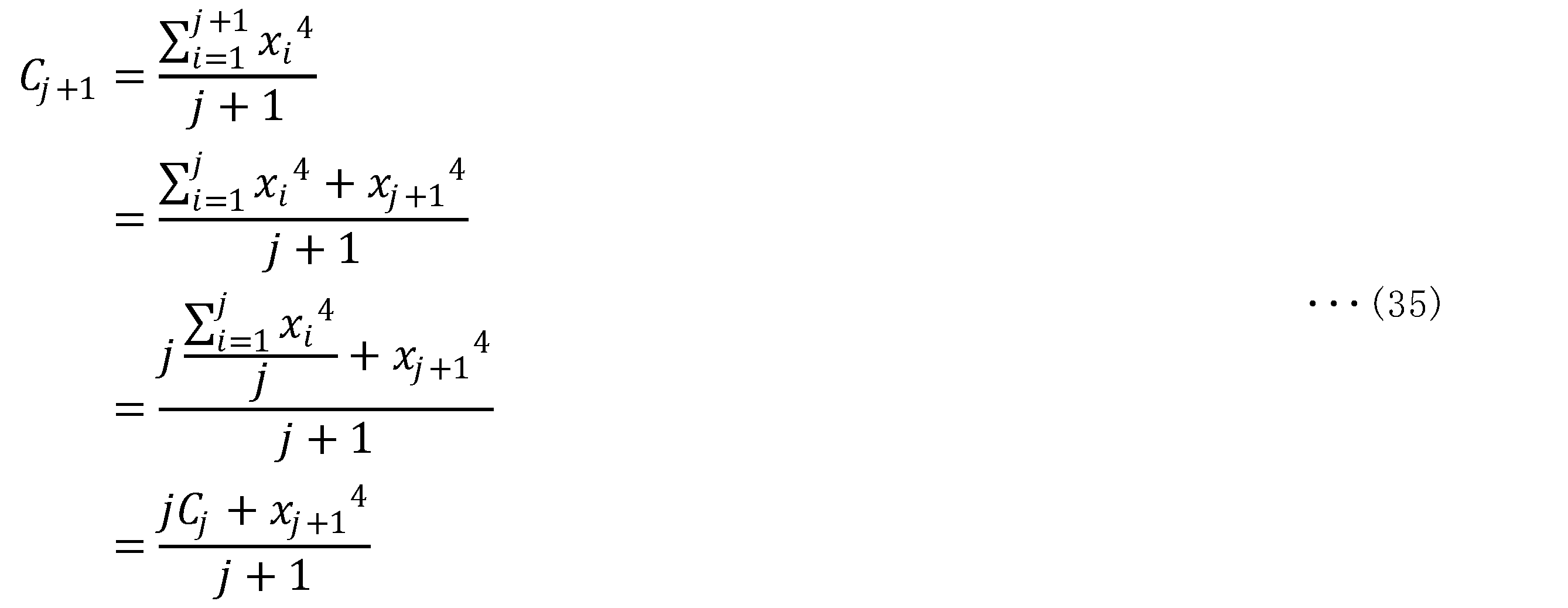















図9は、実施の形態2における情報処理装置2000を含む情報処理システム100Aの構成例を示す図である。図9に示す情報処理システム100Aでは、図1に示す情報処理システム100の構成において、情報処理装置1000が情報処理装置2000に置き替えられ、装置制御部1099が装置制御部2099に置き替えられている。情報処理装置2000では、センサデータ取得部1001がセンサデータ取得部2001に置き替えられ、内部変数計算部1003が内部変数計算部2003に置き替えられ、特徴量計算部1004が特徴量計算部2004に置き替えられている。その他の構成は、図1に示す情報処理システム100と同一又は同等である。なお、同一又は同等の構成部には同一の符号を付すと共に、重複する説明は省略する。
図11は、実施の形態3における情報処理装置3000を含む情報処理システム100Bの構成例を示す図である。図11に示す情報処理システム100Bでは、図9に示す情報処理システム100Aの構成において、情報処理装置2000が情報処理装置3000に置き替えられている。情報処理装置3000では、センサデータ取得部2001がセンサデータ取得部3001に置き替えられ、初期化処理部1005が初期化処理部3005に置き替えられている。その他の構成は、図9に示す情報処理システム100Aと同一又は同等である。なお、同一又は同等の構成部には同一の符号を付すと共に、重複する説明は省略する。
図13は、実施の形態4における情報処理装置4000を含む情報処理システム100Cの構成例を示す図である。図13に示す情報処理システム100Cでは、図11に示す情報処理システム100Bの構成において、情報処理装置3000が情報処理装置4000に置き替えられている。情報処理装置4000では、内部変数計算部1003が内部変数計算部4003に置き替えられ、特徴量計算部1004が特徴量計算部4004に置き替えられ、状態診断部1006が状態診断部4006に置き替えられている。また、新たに収束度計算部4007が設けられている。その他の構成は、図11に示す情報処理システム100Bと同一又は同等である。なお、同一又は同等の構成部には同一の符号を付すと共に、重複する説明は省略する。



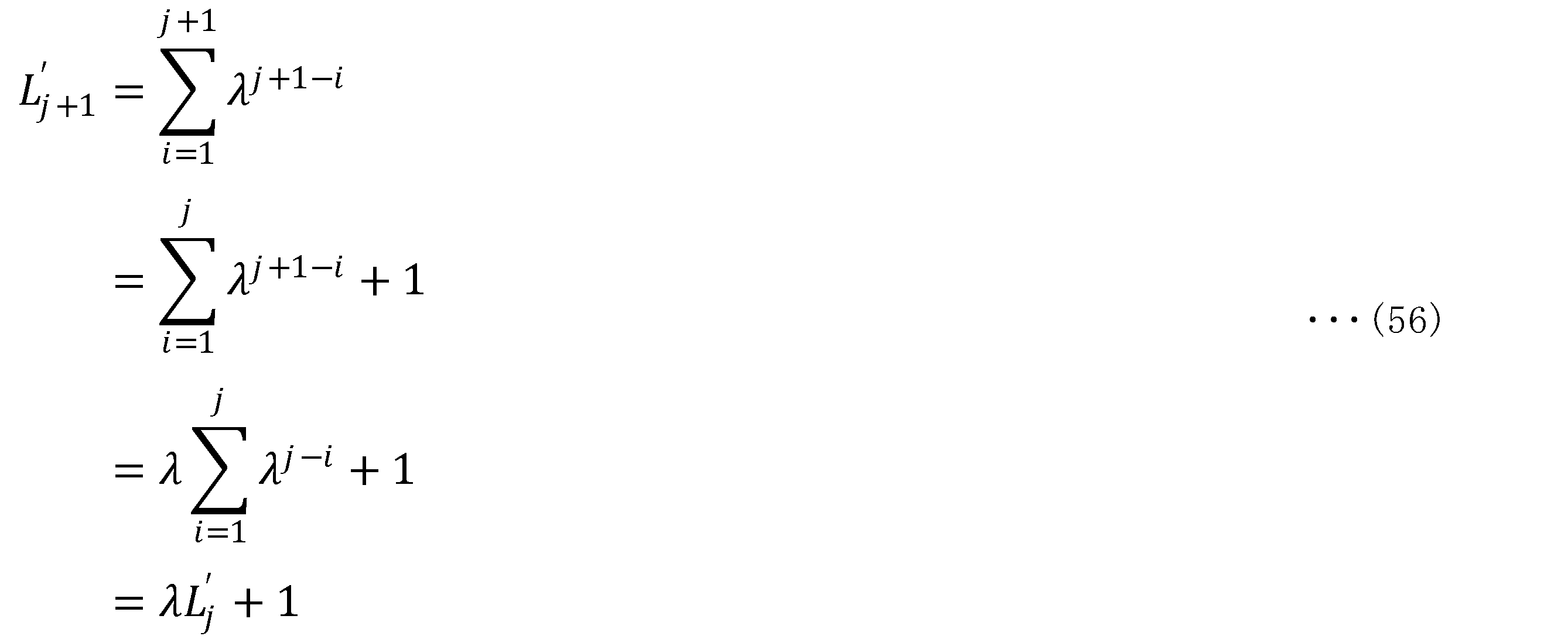








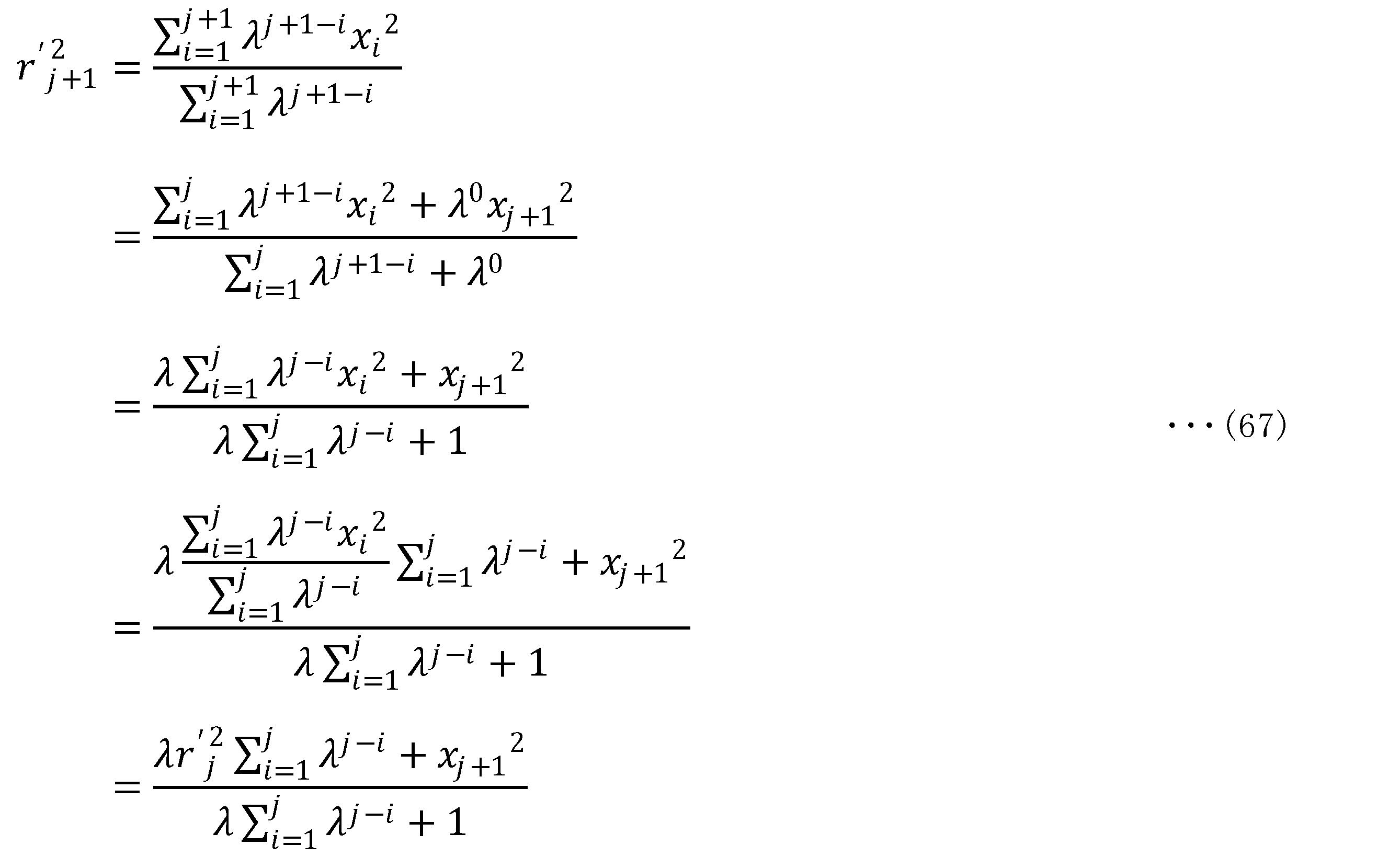

















図16は、実施の形態5における情報処理装置5000を含む情報処理システム100Dの構成例を示す図である。図16に示す情報処理システム100Dでは、図1に示す情報処理システム100の構成において、状態診断部1006が状態診断部5006に置き替えられている。その他の構成は、図1に示す情報処理システム100と同一又は同等である。同一又は同等の構成部には同一の符号を付すと共に、重複する説明は省略する。なお、本実施の形態では、状態診断部5006を図1に示す情報処理装置1000に適用する例で説明するが、図9、図11又は図13に示す、情報処理装置2000,3000,4000のうちの何れに適用してもよい。

図22は、実施の形態6における情報処理装置6000を含む情報処理システム100Eの構成例を示す図である。図22に示す情報処理システム100Eでは、図1に示す情報処理システム100の構成において、状態診断部1006が状態診断部6006に置き替えられている。その他の構成は、図1に示す情報処理システム100と同一又は同等である。同一又は同等の構成部には同一の符号を付すと共に、重複する説明は省略する。なお、本実施の形態では、状態診断部6006を図1に示す情報処理装置1000に適用する例で説明するが、図9、図11又は図13に示す、情報処理装置2000,3000,4000のうちの何れに適用してもよい。
Claims (12)
- センサによって計測された機械装置の物理量の計測値を取得し、前記計測値のうちの第1時点から第N時点(Nは2以上の整数)までの計測値をセンサデータとして保持するセンサデータ取得部と、
前記センサデータに基づいて時系列に順次計算される、前記Nよりも少ない個数の内部変数を保持する内部変数保持部と、
第j+1時点(jは1からN-1までの整数)に対応する前記内部変数を、前記第j+1時点の前記センサデータと第j時点に対応する前記内部変数とに基づいて計算する内部変数計算部と、
前記第N時点の前記内部変数に基づいて前記第1時点から前記第N時点までの前記センサデータに含まれる統計的な特徴を抽出した特徴量を計算する特徴量計算部と、
前記特徴量に基づいて前記機械装置の状態を診断する状態診断部と、
を備える情報処理装置。 - 前記特徴量は、前記センサデータの分散、標準偏差、二乗平均平方根、歪度、及び尖度のうちの少なくとも一つである
請求項1に記載の情報処理装置。 - 前記機械装置はモータによって駆動され、
前記センサデータ取得部は、前記モータの駆動に伴って前記センサで計測される、位置、速度、加速度、動作指令、電流、電圧、トルク、力、圧力、音声、及び光量の計測値のうちの少なくとも一つを前記センサデータとして取得する
請求項1又は2に記載の情報処理装置。 - 前記第1時点の前記内部変数を予め設定した最大値と予め設定した最小値との間の値に決定する初期化処理を実行する初期化処理部を備える
請求項1から3の何れか1項に記載の情報処理装置。 - 前記センサデータ取得部は、前記センサデータを取得する時間の間隔である取得周期、前記機械装置の動作の状況を表す動作信号、及び前記センサデータにおけるデータ値のうちの少なくとも一つに基づいて前記第1時点から前記第j時点までの間の2点以上の時点を決定し、決定した前記2点以上の時点に基づいて内部変数を更新するための計算許可フラグを生成し、
前記内部変数計算部は、前記計算許可フラグの示す各第u時点(uは1以上、且つ前記j以下の整数)について、第u+1時点の前記内部変数を、前記第u時点の前記内部変数の値に決定する
請求項4に記載の情報処理装置。 - 前記センサデータ取得部は、前記センサデータを取得する時間の間隔である取得周期、前記機械装置の動作の状況を表す動作信号、及び前記センサデータのうちの少なくとも一つに基づいて前記第1時点から第N時点までの間の1点以上の時点を決定し、決定した前記1点以上の時点に基づいて内部変数を初期化するための初期化トリガを生成し、
前記初期化処理部は、前記初期化トリガに基づいて前記内部変数を初期化する処理を実行する
請求項4に記載の情報処理装置。 - 前記内部変数計算部は、時刻が古い前記センサデータが前記特徴量に与える影響よりも時刻が新しい前記センサデータのほうが前記特徴量に与える影響を大きくするように重みをつけるための、0より大きく1より小さい忘却係数に基づいて前記内部変数を計算する
請求項1から6の何れか1項に記載の情報処理装置。 - 前記内部変数に基づいて、前記特徴量の計算の収束の度合いを定量的に示す指標である収束度を計算する収束度計算部を備える
請求項7に記載の情報処理装置。 - 前記状態診断部は、
前記特徴量を含む状態量を取得する状態量取得部と、
前記機械装置が正常な状態の状態量に基づいて前記機械装置の状態と前記特徴量との関係を学習する学習部と、
前記学習部が学習した結果に基づいて前記機械装置の異常の度合いを定量的に示す指標である異常度を計算する異常度計算部と、
前記異常度に基づいて前記機械装置の状態を診断した診断結果を決定する意思決定部と、
を備える請求項1から8の何れか1項に記載の情報処理装置。 - 前記状態診断部は、
前記特徴量を含む状態量を取得する状態量取得部と、
前記機械装置の状態と前記状態量との関係を紐付ける学習用データに基づいて前記機械装置の状態と前記状態量との関係を学習する学習部と、
前記学習部に入力された状態量と前記学習部による学習結果とに基づいて前記機械装置の状態を推定する状態推定部と、
前記状態推定部が推定した結果に基づいて前記診断の結果を決定する意思決定部と、
を備える請求項1から9の何れか1項に記載の情報処理装置。 - 機械装置の物理量を計測するセンサから、第1時点から第N時点(Nは2以上の整数)までの各時点における前記物理量の計測値をセンサデータとして取得する第1ステップと、
前記センサデータに基づいて時系列に順次計算される、前記Nよりも少ない個数の内部変数を保持する第2ステップと、
第j+1時点(jは1からN-1までの整数)に対応する前記内部変数を、前記第j+1時点の前記センサデータと第j時点に対応する前記内部変数とに基づいて計算する第3ステップと、
前記第N時点の前記内部変数に基づいて前記第1時点から前記第N時点までの前記センサデータに含まれる統計的な特徴を抽出した特徴量を計算する第4ステップと、
前記特徴量に基づいて前記機械装置の状態を診断する第5ステップと、
を含む情報処理方法。 - 前記第1時点の前記内部変数を予め設定した最大値と最小値との間の値に決定する初期化処理を実行するステップを更に有する
請求項11に記載の情報処理方法。
Priority Applications (7)
| Application Number | Priority Date | Filing Date | Title |
|---|---|---|---|
| US18/031,172 US12498709B2 (en) | 2020-12-18 | 2020-12-18 | Information processing apparatus and information processing method |
| KR1020237018898A KR102841817B1 (ko) | 2020-12-18 | 2020-12-18 | 정보 처리 장치 및 정보 처리 방법 |
| JP2021526355A JP6935046B1 (ja) | 2020-12-18 | 2020-12-18 | 情報処理装置及び情報処理方法 |
| DE112020007851.5T DE112020007851T5 (de) | 2020-12-18 | 2020-12-18 | Informationsverarbeitungsvorrichtung und informationsverarbeitungsverfahren |
| PCT/JP2020/047394 WO2022130611A1 (ja) | 2020-12-18 | 2020-12-18 | 情報処理装置及び情報処理方法 |
| CN202080107328.7A CN116569120A (zh) | 2020-12-18 | 2020-12-18 | 信息处理装置及信息处理方法 |
| TW110146274A TWI814170B (zh) | 2020-12-18 | 2021-12-10 | 資訊處理裝置以及資訊處理方法 |
Applications Claiming Priority (1)
| Application Number | Priority Date | Filing Date | Title |
|---|---|---|---|
| PCT/JP2020/047394 WO2022130611A1 (ja) | 2020-12-18 | 2020-12-18 | 情報処理装置及び情報処理方法 |
Publications (1)
| Publication Number | Publication Date |
|---|---|
| WO2022130611A1 true WO2022130611A1 (ja) | 2022-06-23 |
Family
ID=77657855
Family Applications (1)
| Application Number | Title | Priority Date | Filing Date |
|---|---|---|---|
| PCT/JP2020/047394 Ceased WO2022130611A1 (ja) | 2020-12-18 | 2020-12-18 | 情報処理装置及び情報処理方法 |
Country Status (7)
| Country | Link |
|---|---|
| US (1) | US12498709B2 (ja) |
| JP (1) | JP6935046B1 (ja) |
| KR (1) | KR102841817B1 (ja) |
| CN (1) | CN116569120A (ja) |
| DE (1) | DE112020007851T5 (ja) |
| TW (1) | TWI814170B (ja) |
| WO (1) | WO2022130611A1 (ja) |
Families Citing this family (8)
| Publication number | Priority date | Publication date | Assignee | Title |
|---|---|---|---|---|
| JP2023051402A (ja) * | 2021-09-30 | 2023-04-11 | オムロン株式会社 | 制御システム、情報処理方法および情報処理装置 |
| JP2023065122A (ja) * | 2021-10-27 | 2023-05-12 | 株式会社ジェイテクト | 機械設備及びボールねじ機構の診断方法 |
| JP7638454B2 (ja) * | 2022-09-08 | 2025-03-03 | 三菱電機株式会社 | 異常要因推定装置、学習装置、精密診断システム、および、異常要因推定方法 |
| CN115859201B (zh) * | 2022-11-22 | 2023-06-30 | 淮阴工学院 | 一种化工过程故障诊断方法及系统 |
| JPWO2024134843A1 (ja) * | 2022-12-22 | 2024-06-27 | ||
| WO2024142315A1 (ja) * | 2022-12-27 | 2024-07-04 | 三菱電機株式会社 | 機器診断装置、プログラム、機器診断システム及び機器診断方法 |
| US12594938B2 (en) * | 2023-06-21 | 2026-04-07 | Dana Heavy Vehicle Systems Group, Llc | Optimized electric machine stop position for loss reduction and vehicle launch |
| KR102834176B1 (ko) * | 2023-11-17 | 2025-07-15 | 한국공학대학교산학협력단 | 감속기의 백래시 평가 모델을 생성하는 방법, 감속기의 백래시를 보상하는 방법 및 장치 |
Citations (6)
| Publication number | Priority date | Publication date | Assignee | Title |
|---|---|---|---|---|
| JPH05187965A (ja) * | 1991-08-12 | 1993-07-27 | Kuroda Precision Ind Ltd | ボールねじの寿命監視装置 |
| JP2002341909A (ja) * | 2001-05-18 | 2002-11-29 | Sofutorokkusu:Kk | 工作機器の監視方法 |
| CN102033200A (zh) * | 2009-09-29 | 2011-04-27 | 上海宝钢工业检测公司 | 基于统计模型的交流电机在线监测和诊断方法 |
| WO2013105164A1 (ja) * | 2012-01-13 | 2013-07-18 | 日本電気株式会社 | 異常信号判定装置、異常信号判定方法、および異常信号判定プログラム |
| JP2017162417A (ja) * | 2016-03-11 | 2017-09-14 | 株式会社日立ハイテクノロジーズ | 異常診断装置および方法、並びに、異常診断システム |
| JP2020035372A (ja) * | 2018-08-31 | 2020-03-05 | オムロン株式会社 | 情報処理装置及び情報処理方法 |
Family Cites Families (18)
| Publication number | Priority date | Publication date | Assignee | Title |
|---|---|---|---|---|
| JP2603134B2 (ja) * | 1989-06-06 | 1997-04-23 | 三菱電機株式会社 | 移動平均処理装置 |
| DE10034224B4 (de) * | 2000-07-07 | 2016-11-17 | Continental Teves Ag & Co. Ohg | Verfahren zur Bildung eines Mittelwertes bei der Erkennung eines Druckverlustes in Kraftfahrzeugreifen |
| JP2003329493A (ja) * | 2002-05-14 | 2003-11-19 | Japan Research Institute Ltd | 状態監視方法、状態監視システム、状態監視装置、コンピュータプログラム、及び記録媒体 |
| WO2004063939A2 (de) | 2003-01-10 | 2004-07-29 | Robert Bosch Gmbh | Verfahren zum berechnen eines mittelwertes von messwerten |
| US7075327B2 (en) * | 2003-06-18 | 2006-07-11 | Eaton Corporation | System and method for proactive motor wellness diagnosis |
| JP2008261755A (ja) | 2007-04-12 | 2008-10-30 | Canon Inc | 情報処理装置、情報処理方法 |
| WO2012009804A1 (en) * | 2010-07-23 | 2012-01-26 | Corporation De L'ecole Polytechnique | Tool and method for fault detection of devices by condition based maintenance |
| JP2013191113A (ja) | 2012-03-15 | 2013-09-26 | Sony Corp | 表示制御装置、表示制御方法およびプログラム |
| JP5485441B2 (ja) * | 2013-03-19 | 2014-05-07 | 株式会社日立製作所 | 異常診断装置および産業機械 |
| JP5771317B1 (ja) * | 2014-08-26 | 2015-08-26 | 株式会社日立パワーソリューションズ | 異常診断装置及び異常診断方法 |
| US11327475B2 (en) * | 2016-05-09 | 2022-05-10 | Strong Force Iot Portfolio 2016, Llc | Methods and systems for intelligent collection and analysis of vehicle data |
| WO2018003457A1 (ja) * | 2016-06-30 | 2018-01-04 | パナソニックIpマネジメント株式会社 | 情報処理装置、時系列データの情報処理方法、及びプログラム |
| JP6840953B2 (ja) * | 2016-08-09 | 2021-03-10 | 株式会社リコー | 診断装置、学習装置および診断システム |
| JP6723669B2 (ja) * | 2016-09-27 | 2020-07-15 | 東京エレクトロン株式会社 | 異常検知プログラム、異常検知方法および異常検知装置 |
| JP6842299B2 (ja) * | 2016-12-28 | 2021-03-17 | 三菱パワー株式会社 | 診断装置、診断方法及びプログラム |
| JP7085370B2 (ja) * | 2017-03-16 | 2022-06-16 | 株式会社リコー | 診断装置、診断システム、診断方法およびプログラム |
| DE102017217804A1 (de) * | 2017-10-06 | 2019-04-11 | Bayerische Motoren Werke Aktiengesellschaft | Vorrichtung und verfahren zur ermittlung einer tachometerkennlinie eines fahrzeugs, system zur regelung der geschwindigkeit eines fahrzeugs sowie fahrzeug |
| JP7283485B2 (ja) * | 2018-12-28 | 2023-05-30 | 日本電気株式会社 | 推定装置、推定方法、及びプログラム |
-
2020
- 2020-12-18 US US18/031,172 patent/US12498709B2/en active Active
- 2020-12-18 CN CN202080107328.7A patent/CN116569120A/zh active Pending
- 2020-12-18 KR KR1020237018898A patent/KR102841817B1/ko active Active
- 2020-12-18 DE DE112020007851.5T patent/DE112020007851T5/de active Pending
- 2020-12-18 JP JP2021526355A patent/JP6935046B1/ja active Active
- 2020-12-18 WO PCT/JP2020/047394 patent/WO2022130611A1/ja not_active Ceased
-
2021
- 2021-12-10 TW TW110146274A patent/TWI814170B/zh active
Patent Citations (6)
| Publication number | Priority date | Publication date | Assignee | Title |
|---|---|---|---|---|
| JPH05187965A (ja) * | 1991-08-12 | 1993-07-27 | Kuroda Precision Ind Ltd | ボールねじの寿命監視装置 |
| JP2002341909A (ja) * | 2001-05-18 | 2002-11-29 | Sofutorokkusu:Kk | 工作機器の監視方法 |
| CN102033200A (zh) * | 2009-09-29 | 2011-04-27 | 上海宝钢工业检测公司 | 基于统计模型的交流电机在线监测和诊断方法 |
| WO2013105164A1 (ja) * | 2012-01-13 | 2013-07-18 | 日本電気株式会社 | 異常信号判定装置、異常信号判定方法、および異常信号判定プログラム |
| JP2017162417A (ja) * | 2016-03-11 | 2017-09-14 | 株式会社日立ハイテクノロジーズ | 異常診断装置および方法、並びに、異常診断システム |
| JP2020035372A (ja) * | 2018-08-31 | 2020-03-05 | オムロン株式会社 | 情報処理装置及び情報処理方法 |
Also Published As
| Publication number | Publication date |
|---|---|
| CN116569120A (zh) | 2023-08-08 |
| TW202225886A (zh) | 2022-07-01 |
| US12498709B2 (en) | 2025-12-16 |
| JPWO2022130611A1 (ja) | 2022-06-23 |
| JP6935046B1 (ja) | 2021-09-15 |
| US20230376023A1 (en) | 2023-11-23 |
| TWI814170B (zh) | 2023-09-01 |
| KR102841817B1 (ko) | 2025-08-01 |
| DE112020007851T5 (de) | 2023-09-28 |
| KR20230104236A (ko) | 2023-07-07 |
Similar Documents
| Publication | Publication Date | Title |
|---|---|---|
| JP6935046B1 (ja) | 情報処理装置及び情報処理方法 | |
| JP6810097B2 (ja) | 異常検出器 | |
| CN110187694B (zh) | 故障预测装置以及机器学习装置 | |
| CN106409120B (zh) | 机械学习方法及机械学习装置、以及故障预知装置及系统 | |
| US11235461B2 (en) | Controller and machine learning device | |
| JP6451662B2 (ja) | 異常判定装置、異常判定プログラム、異常判定システム、及びモータ制御装置 | |
| US10684608B2 (en) | Abnormality detection apparatus and machine learning device | |
| CN113219934B (zh) | 自动化系统中的部件的参数设定 | |
| US12103169B2 (en) | Abnormality diagnosis device and abnormality diagnosis method | |
| CN117222878A (zh) | 机器人故障预兆检测装置以及机器人故障预兆检测方法 | |
| US10747197B2 (en) | Abnormally factor identification apparatus | |
| US10802476B2 (en) | Numerical controller with learned pressure estimation | |
| WO2020213062A1 (ja) | モータ制御装置 | |
| JP2021096639A (ja) | 制御方法、制御装置、機械設備、制御プログラム、記録媒体 | |
| CN116635802B (zh) | 数控装置 | |
| US10962957B2 (en) | Collision position estimation device and machine learning device | |
| JP2019024305A (ja) | モータ制御システム | |
| WO2021019760A1 (ja) | 異常診断方法、異常診断装置および異常診断プログラム | |
| JPWO2020152741A1 (ja) | 異常要因推定装置、異常要因推定方法、及びプログラム | |
| JP7011106B1 (ja) | 状態判定装置及び状態判定方法 | |
| US20230191513A1 (en) | Tool diagnostic device | |
| CN114693143A (zh) | 一种数控机床的健康状态评价方法、系统、设备和介质 | |
| JP2022136350A (ja) | 時系列データ解析に基づいたシステム制御 | |
| US12596354B2 (en) | Abnormality information estimation system, operation analysis system, motor control device, abnormality information estimation method, and program | |
| WO2024176390A1 (ja) | データ分割装置、及びコンピュータ読み取り可能な記録媒体 |
Legal Events
| Date | Code | Title | Description |
|---|---|---|---|
| ENP | Entry into the national phase |
Ref document number: 2021526355 Country of ref document: JP Kind code of ref document: A |
|
| 121 | Ep: the epo has been informed by wipo that ep was designated in this application |
Ref document number: 20965998 Country of ref document: EP Kind code of ref document: A1 |
|
| WWE | Wipo information: entry into national phase |
Ref document number: 202327029905 Country of ref document: IN |
|
| WWE | Wipo information: entry into national phase |
Ref document number: 202080107328.7 Country of ref document: CN |
|
| ENP | Entry into the national phase |
Ref document number: 20237018898 Country of ref document: KR Kind code of ref document: A |
|
| WWE | Wipo information: entry into national phase |
Ref document number: 112020007851 Country of ref document: DE |
|
| 122 | Ep: pct application non-entry in european phase |
Ref document number: 20965998 Country of ref document: EP Kind code of ref document: A1 |
|
| WWG | Wipo information: grant in national office |
Ref document number: 202327029905 Country of ref document: IN |
|
| WWG | Wipo information: grant in national office |
Ref document number: 1020237018898 Country of ref document: KR |
|
| WWG | Wipo information: grant in national office |
Ref document number: 18031172 Country of ref document: US |