WO2020031329A1 - 走査型プローブ顕微鏡、および走査型プローブ顕微鏡を用いた物性量測定方法 - Google Patents
走査型プローブ顕微鏡、および走査型プローブ顕微鏡を用いた物性量測定方法 Download PDFInfo
- Publication number
- WO2020031329A1 WO2020031329A1 PCT/JP2018/029917 JP2018029917W WO2020031329A1 WO 2020031329 A1 WO2020031329 A1 WO 2020031329A1 JP 2018029917 W JP2018029917 W JP 2018029917W WO 2020031329 A1 WO2020031329 A1 WO 2020031329A1
- Authority
- WO
- WIPO (PCT)
- Prior art keywords
- sample
- curve
- probe
- displacement
- unit
- Prior art date
- Legal status (The legal status is an assumption and is not a legal conclusion. Google has not performed a legal analysis and makes no representation as to the accuracy of the status listed.)
- Ceased
Links
Images







Classifications
-
- G—PHYSICS
- G01—MEASURING; TESTING
- G01Q—SCANNING-PROBE TECHNIQUES OR APPARATUS; APPLICATIONS OF SCANNING-PROBE TECHNIQUES, e.g. SCANNING PROBE MICROSCOPY [SPM]
- G01Q30/00—Auxiliary means serving to assist or improve the scanning probe techniques or apparatus, e.g. display or data processing devices
- G01Q30/04—Display or data processing devices
-
- G—PHYSICS
- G01—MEASURING; TESTING
- G01Q—SCANNING-PROBE TECHNIQUES OR APPARATUS; APPLICATIONS OF SCANNING-PROBE TECHNIQUES, e.g. SCANNING PROBE MICROSCOPY [SPM]
- G01Q20/00—Monitoring the movement or position of the probe
- G01Q20/02—Monitoring the movement or position of the probe by optical means
-
- B—PERFORMING OPERATIONS; TRANSPORTING
- B82—NANOTECHNOLOGY
- B82Y—SPECIFIC USES OR APPLICATIONS OF NANOSTRUCTURES; MEASUREMENT OR ANALYSIS OF NANOSTRUCTURES; MANUFACTURE OR TREATMENT OF NANOSTRUCTURES
- B82Y35/00—Methods or apparatus for measurement or analysis of nanostructures
-
- G—PHYSICS
- G01—MEASURING; TESTING
- G01Q—SCANNING-PROBE TECHNIQUES OR APPARATUS; APPLICATIONS OF SCANNING-PROBE TECHNIQUES, e.g. SCANNING PROBE MICROSCOPY [SPM]
- G01Q60/00—Particular types of SPM [Scanning Probe Microscopy] or microscopes; Essential components thereof
- G01Q60/24—AFM [Atomic Force Microscopy] or apparatus therefor, e.g. AFM probes
- G01Q60/32—AC mode
-
- G—PHYSICS
- G01—MEASURING; TESTING
- G01Q—SCANNING-PROBE TECHNIQUES OR APPARATUS; APPLICATIONS OF SCANNING-PROBE TECHNIQUES, e.g. SCANNING PROBE MICROSCOPY [SPM]
- G01Q60/00—Particular types of SPM [Scanning Probe Microscopy] or microscopes; Essential components thereof
- G01Q60/24—AFM [Atomic Force Microscopy] or apparatus therefor, e.g. AFM probes
- G01Q60/38—Probes, their manufacture, or their related instrumentation, e.g. holders
Definitions
- the present invention relates to a scanning probe microscope and a method for measuring physical properties using the scanning probe microscope.
- Scanning probe microscopes can measure physical properties such as sample shape, attractive force, adsorption force, and sample hardness by measuring the force curve that represents the distance dependence of the force acting on the probe and the sample surface. . Further, by observing and analyzing the surface state of the sample, the physical properties are measured and imaged while moving the probe in the XY directions. The user can obtain information on the sample such as the unevenness and physical properties from the analysis image.
- the distance dependence of the force acting on the probe and the sample surface changes depending on the sample to be measured. For example, when the sample is soft, the amount of adsorption cannot be measured from the force curve.
- an object of the present invention is to provide a scanning probe microscope capable of measuring a physical quantity representing a physical property of a sample, regardless of the hardness of the sample, and a physical property measuring method using the scanning probe microscope. is there.
- a scanning probe microscope includes a probe, a pointing member for pointing the probe, a placement portion for placing the sample, a driving portion for changing a distance between the sample and the probe, and a pointing member.
- a displacement measuring unit for measuring a displacement of the probe, a first curve representing a relationship between a distance between the probe and the sample when the sample approaches the probe, and an amount representing a displacement of the pointing member;
- a curve creating unit for creating a second curve representing a relationship between a distance between the probe and the sample when moving away from the sample and an amount representing displacement of the pointing member; and a first curve and a second curve.
- a physical quantity calculating unit for obtaining an amount representing an area between them as a physical property quantity of the sample.
- the physical quantity of the sample is an amount representing the hardness of the sample.
- the curve creation unit uses a force received by the pointing member based on the displacement as the amount representing the displacement of the pointing member.
- the driving unit scans the sample or the probe in the horizontal direction.
- the displacement measuring unit measures the displacement of the pointing member at each position in the horizontal direction.
- the curve creating unit creates a first curve and a second curve at each position in the horizontal direction.
- the physical property calculating unit calculates the physical property at each position in the horizontal direction.
- the scanning probe microscope includes an image generation unit that generates an image in which a physical property value for each position in the horizontal direction is a pixel value.
- the physical quantity calculator calculates an area between the first curve and the second curve in a range of a distance between the indicating member and the sample in which the magnitude of the slope of the first curve is equal to or larger than a threshold. Is determined as the physical property of the sample.
- the physical property amount calculation unit is configured to determine an area between the first curve and the second curve in a range of a distance between the indicating member and the sample in which the magnitude of the slope of the second curve is equal to or larger than a threshold. Is determined as the physical property of the sample.
- the physical quantity calculating unit includes: an indicating member and a sample, each of which has a gradient of the first curve equal to or larger than the first threshold and a gradient of the second curve equal to or larger than the second threshold. In the range of the distance between, the amount representing the area between the first curve and the second curve is determined as the physical property of the sample.
- the physical quantity calculating unit obtains, as the physical property of the sample, an amount representing an area between the first curve and the second curve in a range in which the distance between the pointing member and the sample is specified.
- the physical quantity calculating unit obtains the physical quantity for each of the plurality of specified ranges.
- the image generation unit generates a plurality of images having different designated ranges.
- the displacement measuring unit measures the displacement at a plurality of points at a distance between the probe and the sample.
- the physical property calculation unit calculates a difference value between the quantity representing the displacement on the first curve and the quantity representing the displacement on the second curve at each of the plurality of points, and sums the difference values to the physical property quantity of the sample. Asking.
- a scanning probe microscope includes a probe, a pointing member for pointing the probe, a placement portion for placing the sample, a driving portion for changing a distance between the sample and the probe, and a pointing member.
- a displacement measuring unit for measuring the displacement of the sample, a first curve representing a relationship between a distance between the probe and the sample when the sample approaches the probe, and an amount representing a displacement of the pointing member;
- a curve creating section for creating a second curve representing the relationship between the distance between the probe and the sample when moving away from the needle and the amount representing the displacement of the pointing member; and a second or third curve on the first curve.
- a shape value calculating unit for calculating a distance between the pointing member corresponding to the amount representing the designated displacement on the curve and the sample as a shape value representing the surface shape of the sample;
- the driving unit scans the sample or the probe in the horizontal direction.
- the displacement measuring unit measures the displacement of the pointing member at each position in the horizontal direction.
- the curve creating unit creates a first curve and a second curve at each position in the horizontal direction.
- the shape value calculation unit calculates a shape value at each position in the horizontal direction.
- the scanning probe microscope includes an image generation unit that generates an image in which the shape value for each position in the horizontal direction is a pixel value.
- the shape value calculation unit obtains a shape value for each of the plurality of designated displacements.
- the image generation unit generates a plurality of images having different designated displacements.
- the indicating member is a cantilever.
- the present invention is a method for measuring a physical property using a scanning probe microscope including a probe, an indicating member for indicating the probe, a mounting section for mounting a sample, a driving section, and a displacement measuring section.
- the physical property measuring method includes a step in which the driving unit changes the distance between the sample and the probe, a step in which the displacement measuring unit measures the displacement of the pointing member, and a step in which the sample approaches the probe.
- a first curve representing the relationship between the distance between the probe and the sample, and the amount representing the displacement of the pointing member; the distance between the probe and the sample when the sample moves away from the probe; and the displacement of the pointing member.
- a physical quantity representing the physical properties of a sample can be measured regardless of the hardness of the sample.
- FIG. 2 is a diagram illustrating a configuration of a scanning probe microscope 50 according to the first embodiment.
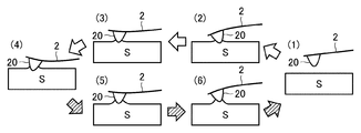
- FIG. 7 is a diagram illustrating displacement of the cantilever 2 when the sample S approaches the cantilever 2 in a vertical direction and when the sample S releases vertically from the cantilever 2.
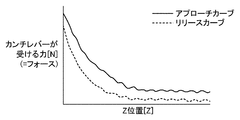
- FIG. 3 is a diagram illustrating an example of a force curve when the cantilever 2 is displaced as in FIG. 2. It is a figure showing another example of a focus curve. It is a figure showing the example of calculation of the amount of elastic recovery.
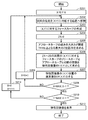
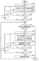
- 5 is a flowchart illustrating a procedure for generating a surface shape image according to the first embodiment.
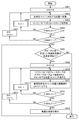
- 5 is a flowchart illustrating a procedure of generating an elastic recovery image according to the first embodiment.
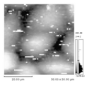
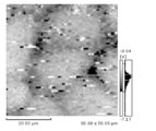
- FIG. 4 is a diagram illustrating an example of a surface shape image when a sample S is HeLa cells.
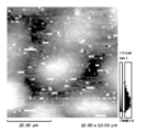
- FIG. 4 is a diagram illustrating an example of an elastic recovery image when a sample S is HeLa cells. It is a flowchart showing the generation
- 11 is a flowchart illustrating a procedure for generating a surface shape image according to the third embodiment. It is a figure showing the example of specification of the force FA of a force curve.
- FIG. 7 is a diagram illustrating an example of a surface shape image for a first force FA1 when a sample S is HeLa cells.
- FIG. 3 is a diagram illustrating an example of a hardware configuration of a measurement unit.
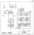
- FIG. 1 is a diagram illustrating a configuration of a scanning probe microscope 50 according to the first embodiment.
- the scanning probe microscope 50 includes a scanner 43, a probe 20, a cantilever 2, a displacement measuring unit 3, an A / D converter 35, a measuring unit 1, and a driving unit 4. , A display device 51.
- the scanner 43 places the sample S thereon and is driven by the drive unit 4 in a three-dimensional direction.
- the cantilever 2 supports the probe 20.
- the cantilever 2 is displaced by an atomic force (attraction or repulsion) between the probe 20 and the sample S.
- the displacement measuring unit 3 detects the deflection of the cantilever 2.
- the displacement measuring unit 3 includes a light source 31, mirrors 32 and 33, and a photodetector.
- the light source 31 includes a laser oscillator that emits a laser beam.
- the mirrors 32 and 33 constitute an optical system.
- the photodetector 34 is configured by a photodiode or the like that detects an incident laser beam.
- the laser light emitted from the light source 31 is reflected by the mirror 32 and enters the cantilever 2.
- the laser light is reflected by the cantilever 2, further reflected by the mirror 33, and made incident on the photodetector 34.
- the displacement of the cantilever 2 can be measured by the photodetector 34 detecting the laser beam.
- the A / D converter 35 converts the displacement signal detected by the light detector 34 into a digital signal.
- the measuring unit 1 includes a force curve creating unit 11, a shape value calculating unit 52, a surface shape image generating unit 12, a physical property calculating unit 53, and a physical property image generating unit 13.
- the force curve creating unit 11 creates a force curve representing a time change of the acting force (force) from a time change of the displacement of the cantilever 2.
- the force curve creation unit 11 multiplies the displacement D [V] of the cantilever 2 by the spring constant K [N / m] and the sensitivity S [m / V], thereby obtaining the force [N]. calculate.
- the spring constant K is a spring constant of a spring connected to the probe 20.
- the sensitivity is the reciprocal of the slope of the force curve when a force curve is created with a hard sample without deformation.
- the shape value calculator 52 calculates the shape value of the sample S from the force curve.
- the surface shape image generation unit 12 generates a surface shape image in which the shape value at each location obtained by scanning the sample S on the XY plane (horizontal direction) by the scanner 43 is a pixel value.
- the physical property amount calculation unit 53 calculates the elastic recovery amount as the physical property amount of the sample S from the force curve.
- the elastic recovery amount is an amount indicating how quickly the dent of the sample S returns to its original shape when the probe 20 is pushed into the sample S to dent the sample S, and then the probe 20 is separated from the sample S. The softer the sample S, the greater the elastic recovery. Therefore, the elastic recovery amount is also an amount representing the hardness of the sample S.
- the physical property image generation unit 13 generates an elastic recovery image in which the amount of elastic recovery at each location obtained by scanning the sample S on the XY plane (horizontal direction) by the scanner 43 is a pixel value.
- the measurement unit 1 outputs a control signal to the drive unit 4.
- the drive unit 4 includes a D / A converter 41 and a scanner driver 42.
- the D / A converter 41 converts a digital control signal from the measuring unit 1 into an analog signal and sends the analog signal to the scanner driver 42.
- the scanner driver 42 can scan the sample S by receiving the control signal and driving the scanner 43 in the X-axis direction, the Y-axis direction, and the Z-axis direction.
- the Z-axis direction is a vertical direction
- the XY plane is a horizontal plane.
- the drive unit 4 moves the sample S in the X direction and the Y direction in the range of several tens ⁇ m to several tens nm.
- FIG. 2 is a diagram showing the displacement of the cantilever 2 when the sample S approaches the probe 20 in the vertical direction and when the sample S is released from the probe 20 in the vertical direction.
- FIG. 3 is a diagram illustrating an example of a force curve when the cantilever 2 is displaced as in FIG. 3, the horizontal axis represents the vertical position Z of the sample S with the position of the probe 20 as the origin.
- the vertical position Z represents the vertical distance between the probe 20 and the sample S.
- the vertical axis in FIG. 2 represents the force, that is, the force received by the cantilever 2.
- the probe 20 at the tip of the cantilever 2 is completely separated from the sample S.
- the cantilever 2 receives a slight attractive force from the sample S and warps downward. This is called jump-in.
- the cantilever 2 receives a repulsive force and warps upward.
- the probe 20 and the sample S come in closest contact with each other, and the repulsive force becomes maximum.
- the force received by the cantilever 2 changes from repulsive force to attractive force.
- an attractive force acts between the cantilever 2 and the sample S, and the attractive force is maximized.
- the probe 20 separates from the sample S and returns to the state of (1). This is called jump-out.
- the force curve in FIG. 3 is composed of an approach curve at the time of approach and a release curve at the time of release.
- the surface shape image is an image in which the value Z0 of the Z position with respect to a certain force F0 on the approach curve is a pixel value. Further, the amount of adsorption can be measured from the difference between the start point (minimum value) and the end point (maximum value) of the force F at the time of jump-out.
- FIG. 4 is a diagram illustrating another example of the focus curve. For example, when the sample S is soft, jump-in and jump-out do not occur in the force curve as shown in FIG. When the sample S is soft, jump-out does not occur, so that the adsorption force cannot be measured.
- the physical property calculation unit 53 calculates the elastic recovery amount from the force curve as the physical property of the sample S.
- the amount representing the area between the approach curve and the release curve is determined as the elastic recovery amount of the sample S.
- the physical property calculation unit 53 obtains an amount representing an area between the approach curve and the release curve in a range of the distance between the probe 20 and the sample S in which the magnitude of the slope of the approach curve is equal to or larger than the threshold TH1. You may.
- the physical property calculation unit 53 calculates the distance between the probe 20 and the sample S where the gradient of the approach curve is equal to or larger than the threshold value TH1. In the range, the difference value ⁇ F between the force F1 on the approach curve and the force F2 on the release curve at each sample point at the distance between the probe 20 and the sample S is obtained, and the sum of the difference values ⁇ F is used as the elastic recovery amount. You may ask for it.
- FIG. 5 is a diagram illustrating a calculation example of the elastic recovery amount. As shown in FIG. 5, the area between the approach curve and the release curve can be obtained as the elastic recovery amount in the range of ZA to ZB.
- the range of ZA to ZB is a range where the magnitude of the slope of the approach curve is equal to or larger than the threshold value TH1.
- FIG. 6 is a flowchart showing a procedure for generating a surface shape image according to the first embodiment.
- the size of the surface shape image is X_MAX ⁇ Y_MAX.
- step S101 the surface shape image generation unit 12 sets the pixel position (X, Y) of the surface shape image to (0, 0).
- step S102 the drive unit 4 moves the horizontal position of the sample S to a position corresponding to (X, Y).
- step S103 the force curve creating unit 11 creates a force curve for (X, Y).
- step S104 the shape value calculation unit 52 obtains, as a shape value, a Z position Z0 (X, Y) with respect to a certain force F0 on an approach curve forming a force curve for (X, Y).
- step S105 the surface shape image generation unit 12 sets the pixel value at the pixel position (X, Y) of the surface shape image as the shape value Z0 (X, Y).
- step S107 the surface shape image generation unit 12 increments X. Thereafter, the process returns to step S102.
- step S110 the surface shape image generation unit 12 displays the surface shape image on the display device 51.
- FIG. 7 is a flowchart showing a procedure for generating an elastic recovery image according to the first embodiment. Let X_MAX ⁇ Y_MAX be the size of the elastic recovery image.
- step S201 the physical property image generation unit 13 sets the pixel position (X, Y) of the elasticity recovery image to (0, 0).
- step S202 the driving unit 4 moves the horizontal position of the sample S to a position corresponding to (X, Y).
- step S203 the force curve creating unit 11 creates a force curve for (X, Y).
- step S204 the physical property calculation unit 53 sets the minimum value “0” of the Z position of the force curve for (X, Y) as the starting point ZA.
- step S205 the physical property calculation unit 53 obtains, as the end point ZB, the maximum value of the Z position where the magnitude of the slope of the approach curve forming the force curve for (X, Y) is equal to or larger than the threshold value TH1. In the range from the start point ZA to the end point ZB, the magnitude of the slope of the approach curve is equal to or larger than the threshold value TH1.
- step S206 the physical property calculation unit 53 obtains the area between the approach curve and the release curve in the section where the Z position is between ZA and ZB as the elastic recovery amount ER (X, Y).
- step S207 the physical property image generation unit 13 sets the pixel value at the pixel position (X, Y) of the elastic recovery image as the elastic recovery amount ER (X, Y).
- step S209 the physical quantity image generation unit 13 increments X. Thereafter, the process returns to step S202.
- step S212 the physical property image generation unit 13 displays the elasticity recovery image on the display device 51.
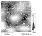
- FIG. 8 is a diagram illustrating an example of a surface shape image when the sample S is HeLa cells. As shown in FIG. 8, the shape of the HeLa cell can be known from the surface shape image.
- FIG. 9 is a diagram illustrating an example of an elastic recovery image when the sample S is HeLa cells.
- the elastic recovery image shows the amount of elastic recovery inside the HeLa cell (that is, when the HeLa cell is depressed with the probe 20 and the probe 20 is released from the HeLa cell, The amount that indicates how quickly the dent returns).
- the elastic recovery amount is obtained in a specified range of the Z position of the force curve.
- FIG. 10 is a flowchart showing a procedure for generating an elastic recovery image according to the second embodiment. Let X_MAX ⁇ Y_MAX be the size of the elastic recovery image.
- step S301 the physical property image generation unit 13 sets the pixel position (X, Y) of the elasticity recovery image to (0, 0).
- step S302 the drive unit 4 moves the horizontal position of the sample S to a position corresponding to (X, Y).
- step S303 the force curve creating unit 11 creates a force curve for (X, Y).
- step S305 the physical quantity image generation unit 13 increments X. Thereafter, the process returns to step S302.
- step S308 when there is a request to generate an elastic recovery image specifying the range of the Z position of the force curve (start point ZA and end point ZB), the process proceeds to step S309. If there is no request to generate an elastic recovery image, the process ends.
- step S309 the physical property image generation unit 13 sets the pixel position (X, Y) of the elastic recovery image to (0, 0).
- step S310 the physical property calculation unit 53 calculates the area between the approach curve and the release curve in the section where the Z position of the force curve for (X, Y) is between ZA and ZB, and calculates the elastic recovery amount ER (X, Y).
- step S311 the physical property image generation unit 13 sets the pixel value at the pixel position (X, Y) of the elastic recovery image as the elastic recovery amount ER (X, Y).
- step S312 the physical property image generation unit 13 increments X. Thereafter, the process returns to step S310.
- step S316 the physical property image generation unit 13 displays the elasticity recovery image on the display device 51. Thereafter, the process returns to step S308.
- FIG. 11 is a diagram illustrating an example of specifying the range of the Z position of the force curve.
- the first range is a range where the start point is ZA (1) and the end point is ZB (1).
- the second range is a range where the start point is ZA (2) and the end point is ZB (2).
- step S308 when there is a request to generate a plurality of elastic recovery images in which the designation of the range of the Z position of the force curve (start point ZA and end point ZB) is different, the physical property amount calculation unit 53 sets the plurality of designated ranges. , The amount of elastic recovery (X, Y) is determined. The physical property image generation unit 13 generates a plurality of elastic recovery images having different designated ranges. As shown in FIG. 11, when the first range and the second range are designated, two elastic recovery images having different designated ranges are obtained.
- FIG. 12 is a flowchart showing a procedure for generating a surface shape image according to the third embodiment.
- the size of the surface shape image is X_MAX ⁇ Y_MAX.
- step S401 the surface shape image generation unit 12 sets the pixel position (X, Y) of the surface shape image to (0, 0).
- step S402 the drive unit 4 moves the horizontal position of the sample S to a position corresponding to (X, Y).
- step S403 the force curve creation unit 11 generates a force curve for (X, Y).
- step S405 the surface shape image generation unit 12 increments X. Thereafter, the process returns to step S402.
- step S408 if there is a request to generate a surface shape image designating the force FA of the force curve, the process proceeds to step S409. If there is no request to generate a surface shape image, the process ends.
- step S409 the surface shape image generation unit 12 sets the pixel position (X, Y) of the surface shape image to (0, 0).
- step S410 the shape value calculation unit 52 obtains a Z position ZA (X, Y) with respect to the force FA on the approach curve of the force curve for (X, Y) as a shape value.
- step S411 the surface shape image generation unit 12 sets the pixel value at the pixel position (X, Y) of the surface shape image as the shape value ZA (X, Y).
- step S413 the surface shape image generation unit 12 increments X. Thereafter, the process returns to step S410.
- step S416 the surface shape image generation unit 12 displays the surface shape image on the display device 51. Thereafter, the process returns to step S408.
- FIG. 13 is a diagram illustrating an example of specifying a force FA of a force curve.
- a first force FA1 and a second force FA2 are designated.
- step S408 when there is a request to generate a plurality of surface shape images with different designations of the force FA of the force curve, the shape value calculation unit 52 determines the shape value ZA ( X, Y).
- the surface shape image generation unit 12 generates a plurality of surface shape images having different designated forces. As shown in FIG. 13, when the first force and the second force are specified, two surface shape images having different forces are obtained.
- FIG. 14 is a diagram illustrating an example of a surface shape image with respect to the first force FA1 when the sample S is HeLa cells.
- FIG. 15 is a diagram illustrating an example of a surface shape image with respect to the second force FA2 when the sample S is HeLa cells.
- a difference in force that is, a difference in force for pushing HeLa cells results in a different surface shape image.
- the cell is deformed by gradually changing the force FA as the pushing force to create a plurality of surface shape images and displaying the plurality of surface shape images continuously like a moving image. You can also show the situation.
- FIG. 16 is a diagram illustrating a configuration of a scanning probe microscope 550 according to the fourth embodiment.
- the scanning probe microscope 550 of the fourth embodiment includes a displacement curve creation unit 91 instead of the force curve creation unit 11.
- the force curve creating unit 11 calculates the force by multiplying the displacement D [V] of the cantilever 2 by the spring constant K [N / m] and the sensitivity S [m / V]. Created a force curve.
- the displacement curve creation unit 91 creates a displacement curve representing a time change of the displacement of the cantilever 2.
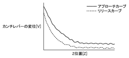
- FIG. 17 is a diagram illustrating an example of a displacement curve.
- the horizontal axis represents the vertical position Z of the sample S with the probe 20 as the origin.
- the vertical position Z represents the vertical distance between the probe 20 and the sample S.
- the vertical axis in FIG. 16 represents the displacement of the cantilever 2.
- the displacement curve of the present embodiment has the same shape as the force curve. Therefore, the shape value and the amount of elastic recovery described in the first to third embodiments can also be obtained from a displacement curve.
- the shape value calculation unit 52 calculates the shape value using the displacement curve in the same way as calculating the shape value using the force curve.
- the physical property amount calculation unit 53 calculates the elastic recovery amount using the displacement curve in the same manner as the calculation of the elastic recovery amount using the force curve.
- the Z position with respect to a certain force F on the approach curve is used as the shape value, but the present invention is not limited to this.
- the Z position for a certain force F on the release curve may be used as the shape value.
- the Z position for a certain force F on the approach curve and the Z position for a certain force F on the release curve may be used as the shape values.
- the physical property amount calculation unit 53 determines the maximum value of the Z position at which the magnitude of the slope of the approach curve forming the force curve is equal to or larger than the threshold value TH1 as an end point for area calculation. Although determined as ZB, it is not limited to this.
- the physical property amount calculation unit 53 may obtain the maximum value of the Z position where the magnitude of the slope of the release curve constituting the force curve is equal to or larger than the threshold value TH2 as the end point ZB for the area calculation.
- the physical property amount calculation unit 53 determines the maximum of the Z position where the magnitude of the slope of the approach curve forming the force curve is equal to or greater than the threshold value TH1 and the magnitude of the slope of the release curve configuring the force curve is equal to or greater than the threshold value TH2.
- the value may be obtained as the end point ZB for calculating the area.
- the threshold value TH1 and the threshold value TH2 may be the same.
- the driving unit moves the sample S in the three-dimensional direction.
- the driving unit may move the probe 20 in the three-dimensional direction.
- FIG. 18 is a diagram illustrating an example of a hardware configuration of a measurement unit.
- the force curve creating unit 11, the shape value calculating unit 52, the surface shape image generating unit 12, the physical property calculating unit 53, and the physical property image generating unit 13 constituting the measuring unit 1 of FIG. 1100 and a memory 1200 connected by a bus 1300.
- the control unit 40 is realized by a processor 1110 such as a CPU (Central Processing Unit) executing a program stored in the memory 1200. Further, a plurality of processors and a plurality of memories may cooperate to execute the functions of the above components. The same applies to the displacement curve creating section 91, the shape value calculating section 52, the surface shape image generating section 12, the physical property calculating section 53, and the physical property image generating section 13, which constitute the measuring section 81 of FIG.
Landscapes
- Physics & Mathematics (AREA)
- Health & Medical Sciences (AREA)
- General Health & Medical Sciences (AREA)
- General Physics & Mathematics (AREA)
- Nuclear Medicine, Radiotherapy & Molecular Imaging (AREA)
- Radiology & Medical Imaging (AREA)
- Chemical & Material Sciences (AREA)
- Engineering & Computer Science (AREA)
- Nanotechnology (AREA)
- Analytical Chemistry (AREA)
- Crystallography & Structural Chemistry (AREA)
- Power Engineering (AREA)
- Length Measuring Devices With Unspecified Measuring Means (AREA)
Abstract
Description
好ましくは、カーブ作成部は、指示部材の変位を表わす量として、変位に基づく指示部材が受ける力を用いる。
本発明は、探針と、探針を指示する指示部材と、試料を載置する載置部と、駆動部と、変位測定部と備えた走査型プローブ顕微鏡を用いた物性量測定方法である。物性量測定方法は、駆動部が、試料と探針との間の距離を変化させるステップと、変位測定部が、指示部材の変位を測定するステップと、試料が探針に近づくときの探針と試料との間の距離と、指示部材の変位を表わす量との関係を表わす第1のカーブと、試料が探針から遠ざかるときの探針と試料との間の距離と、指示部材の変位を表わす量との関係を表わす第2のカーブとを作成するステップと、第1のカーブと第2のカーブとの間の面積を表わす量を試料の物性量として求めるステップとを備える。
[第1の実施形態]
図1は、第1の実施形態の走査型プローブ顕微鏡50の構成を表わす図である。
カンチレバー2は、探針20を支持する。探針20と試料Sとの間の原子間力(引力または斥力)によって、カンチレバー2が変位する。
表面形状像生成部12は、スキャナ43によって試料SをXY平面(水平方向)で走査することによって得られる各場所での形状値を画素値とした表面形状像を生成する。
駆動部4は、D/A変換器41と、スキャナドライバ42とを備える。D/A変換器41は、測定部1からのデジタルの制御信号をアナログ信号に変換して、スキャナドライバ42に送る。
たとえば試料Sが柔らかい場合には、図4に示すように、フォースカーブにジャンプインおよびジャンプアウトが発生しない。試料Sが柔らかい場合には、ジャンプアウトが発生しないので、吸着力を測定することができない。
図5に示すように、ZA~ZBの範囲において、アプローチカーブとリリースカーブとの間の面積が弾性回復量として求めることができる。ZA~ZBの範囲は、アプローチカーブの傾きの大きさが閾値TH1以上となる範囲である。
図8に示すように、表面形状像によって、HeLa細胞の形状を知ることができる。
図9に示すように、弾性回復像によって、HeLa細胞の内部の弾性回復量(すなわち、探針20でHeaLa細胞を凹ませた後、探針20をHeLa細胞から離したときに、HeLa細胞の凹みがどれだけ早く元に戻るかを表わす量)を知ることができる。
第2の実施形態では、フォースカーブのZ位置の指定された範囲で弾性回復量を求める。
第1の範囲は、始点をZA(1)、終点をZB(1)とする範囲である。第2の範囲は、始点をZA(2)、終点をZB(2)とする範囲である。
第3の実施形態では、フォースカーブの指定されたフォースでの形状値を求める。
図13では、第1のフォースFA1と第2のフォースFA2が指定されている。
図16は、第4の実施形態の走査型プローブ顕微鏡550の構成を表わす図である。
図17において、横軸は、探針20を原点とした試料Sの垂直方向の位置Zを表わす。垂直方向の位置Zは、探針20と試料Sの垂直方向の距離を表わす。図16の縦軸は、カンチレバー2の変位を表わす。
本発明は、上記の実施形態に限定されるものではなく、たとえば、以下のような変形例も含む。
上記の実施形態では、アプローチカーブ上のあるフォースFに対するZ位置を形状値としたが、これに限定されるものではない。たとえば、リリースカーブ上のあるフォースFに対するZ位置を形状値としてもよい。あるいは、アプローチカーブ上のあるフォースFに対するZ位置と、リリースカーブ上のあるフォースFに対するZ位置を形状値としてもよい。
第1の実施形態では、物性量算出部53は、フォースカーブを構成するアプローチカーブの傾きの大きさが閾値TH1以上となるZ位置の最大値を面積計算のための終点ZBとして求めたが、これに限定されるものではない。物性量算出部53は、フォースカーブを構成するリリースカーブの傾きの大きさが閾値TH2以上となるZ位置の最大値を面積計算のための終点ZBとして求めてもよい。あるいは、物性量算出部53は、フォースカーブを構成するアプローチカーブの傾きの大きさが閾値TH1以上、かつ、フォースカーブを構成するリリースカーブの傾きの大きさが閾値TH2以上となるZ位置の最大値を面積計算のための終点ZBとして求めてもよい。上記において、閾値TH1と閾値TH2は、同一であってもよい。
上記の実施形態では、駆動部が、試料Sを3次元方向に移動させたが、これに限定するものではない。駆動部が、探針20を3次元方向に移動させるものとしてもよい。
図18は、測定部のハードウエア構成の例を表わす図である。
Claims (13)
- 探針と、
前記探針を指示する指示部材と、
試料を載置する載置部と、
前記試料と前記探針との間の距離を変化させる駆動部と、
前記指示部材の変位を測定する変位測定部と、
前記試料が前記探針に近づくときの前記探針と前記試料との間の距離と前記指示部材の変位を表わす量との関係を表わす第1のカーブと、前記試料が前記探針から遠ざかるときの前記探針と前記試料との間の距離と前記指示部材の変位を表わす量との関係を表わす第2のカーブとを作成するカーブ作成部と、
前記第1のカーブと前記第2のカーブとの間の面積を表わす量を前記試料の物性量として求める物性量算出部とを備える、走査型プローブ顕微鏡。 - 前記試料の物性量は、前記試料の固さを表わす量である、請求項1記載の走査型プローブ顕微鏡。
- 前記カーブ作成部は、前記指示部材の変位を表わす量として、前記変位に基づく前記指示部材が受ける力を用いる、請求項2記載の走査型プローブ顕微鏡。
- 前記駆動部は、前記試料または前記探針を水平方向に走査し、
前記変位測定部は、前記水平方向の各位置での前記指示部材の変位を測定し、
前記カーブ作成部は、前記水平方向の各位置での前記第1のカーブおよび前記第2のカーブを作成し、
前記物性量算出部は、前記水平方向の各位置での前記物性量を求め、
前記水平方向の各位置に対する前記物性量を画素値とした画像を生成する画像生成部を備える、請求項2記載の走査型プローブ顕微鏡。 - 前記物性量算出部は、前記第1のカーブの傾きの大きさが閾値以上となる前記指示部材と前記試料との間の距離の範囲において、前記第1のカーブと前記第2のカーブとの間の面積を表わす量を前記試料の物性量として求める、請求項4記載の走査型プローブ顕微鏡。
- 前記物性量算出部は、前記第2のカーブの傾きの大きさが閾値以上となる前記指示部材と前記試料との間の距離の範囲において、前記第1のカーブと前記第2のカーブとの間の面積を表わす量を前記試料の物性量として求める、請求項4記載の走査型プローブ顕微鏡。
- 前記物性量算出部は、前記第1のカーブの傾きの大きさが第1の閾値以上であり、かつ前記第2のカーブの傾きの大きさが第2の閾値以上となる前記指示部材と前記試料との間の距離の範囲において、前記第1のカーブと前記第2のカーブとの間の面積を表わす量を前記試料の物性量として求める、請求項4記載の走査型プローブ顕微鏡。
- 前記物性量算出部は、前記指示部材と前記試料との間の距離が指定された範囲において、前記第1のカーブと前記第2のカーブとの間の面積を表わす量を前記試料の物性量として求める、請求項4記載の走査型プローブ顕微鏡。
- 前記物性量算出部は、複数の前記指定された範囲に対して、それぞれ前記物性量を求め、
前記画像生成部は、前記指定された範囲が異なる複数の前記画像を生成する、請求項8記載の走査型プローブ顕微鏡。 - 前記変位測定部は、前記探針と前記試料との間の距離の複数のポイントで変位を測定し、
前記物性量算出部は、前記複数のポイントの各々おける前記第1のカーブ上の変位を表わす量と前記第2のカーブ上の変位を表わす量との差分値を算出し、前記差分値の総和を前記試料の物性量として求める、請求項1記載の走査型プローブ顕微鏡。 - 探針と、
前記探針を指示する指示部材と、
試料を載置する載置部と、
前記試料と前記探針との間の距離を変化させる駆動部と、
前記指示部材の変位を測定する変位測定部と、
前記試料が前記探針に近づくときの前記探針と前記試料との間の距離と、前記指示部材の変位を表わす量との関係を表わす第1のカーブと、前記試料が前記探針から遠ざかるときの前記探針と前記試料との間の距離と、前記指示部材の変位を表わす量との関係を表わす第2のカーブとを作成するカーブ作成部と、
前記第1のカーブ上または前記第2のカーブ上の指定された変位を表わす量に対応する前記指示部材と前記試料との間の距離を前記試料の表面形状を表わす形状値として求める形状値算出部とを備え、
前記駆動部は、前記試料または前記探針を水平方向に走査し、
前記変位測定部は、前記水平方向の各位置での前記指示部材の変位を測定し、
前記カーブ作成部は、前記水平方向の各位置での前記第1のカーブおよび前記第2のカーブを作成し、
前記形状値算出部は、前記水平方向の各位置での前記形状値を求め、
前記水平方向の各位置に対する前記形状値を画素値とした画像を生成する画像生成部を備え、
前記形状値算出部は、複数の前記指定された変位に対して、それぞれ前記形状値を求め、
前記画像生成部は、前記指定された変位が異なる複数の前記画像を生成する、走査型プローブ顕微鏡。 - 前記指示部材は、カンチレバーである、請求項1または11記載の走査型プローブ顕微鏡。
- 探針と、前記探針を指示する指示部材と、試料を載置する載置部と、駆動部と、変位測定部と備えた走査型プローブ顕微鏡を用いた物性量測定方法であって、
前記駆動部が、前記試料と前記探針との間の距離を変化させるステップと、
前記変位測定部が、前記指示部材の変位を測定するステップと、
前記試料が前記探針に近づくときの前記探針と前記試料との間の距離と、前記指示部材の変位を表わす量との関係を表わす第1のカーブと、前記試料が前記探針から遠ざかるときの前記探針と前記試料との間の距離と、前記指示部材の変位を表わす量との関係を表わす第2のカーブとを作成するステップと、
前記第1のカーブと前記第2のカーブとの間の面積を表わす量を前記試料の物性量として求めるステップとを備える、走査型プローブ顕微鏡を用いた物性量測定方法。
Priority Applications (4)
| Application Number | Priority Date | Filing Date | Title |
|---|---|---|---|
| CN201880096598.5A CN112567252B (zh) | 2018-08-09 | 2018-08-09 | 扫描探针显微镜以及使用扫描探针显微镜的物理性质测定方法 |
| PCT/JP2018/029917 WO2020031329A1 (ja) | 2018-08-09 | 2018-08-09 | 走査型プローブ顕微鏡、および走査型プローブ顕微鏡を用いた物性量測定方法 |
| US17/266,648 US12352779B2 (en) | 2018-08-09 | 2018-08-09 | Scanning probe microscope and method for measuring physical quantity using scanning probe microscope |
| JP2020535425A JP7001166B2 (ja) | 2018-08-09 | 2018-08-09 | 走査型プローブ顕微鏡、および走査型プローブ顕微鏡を用いた物性量測定方法 |
Applications Claiming Priority (1)
| Application Number | Priority Date | Filing Date | Title |
|---|---|---|---|
| PCT/JP2018/029917 WO2020031329A1 (ja) | 2018-08-09 | 2018-08-09 | 走査型プローブ顕微鏡、および走査型プローブ顕微鏡を用いた物性量測定方法 |
Publications (1)
| Publication Number | Publication Date |
|---|---|
| WO2020031329A1 true WO2020031329A1 (ja) | 2020-02-13 |
Family
ID=69414058
Family Applications (1)
| Application Number | Title | Priority Date | Filing Date |
|---|---|---|---|
| PCT/JP2018/029917 Ceased WO2020031329A1 (ja) | 2018-08-09 | 2018-08-09 | 走査型プローブ顕微鏡、および走査型プローブ顕微鏡を用いた物性量測定方法 |
Country Status (4)
| Country | Link |
|---|---|
| US (1) | US12352779B2 (ja) |
| JP (1) | JP7001166B2 (ja) |
| CN (1) | CN112567252B (ja) |
| WO (1) | WO2020031329A1 (ja) |
Cited By (2)
| Publication number | Priority date | Publication date | Assignee | Title |
|---|---|---|---|---|
| WO2025032942A1 (ja) * | 2023-08-10 | 2025-02-13 | 株式会社島津製作所 | 走査型プローブ顕微鏡およびカンチレバーの評価方法 |
| WO2026009551A1 (ja) * | 2024-07-05 | 2026-01-08 | 株式会社島津製作所 | 光検出装置、走査型プローブ顕微鏡、および測定方法 |
Citations (3)
| Publication number | Priority date | Publication date | Assignee | Title |
|---|---|---|---|---|
| JPH06307850A (ja) * | 1993-04-26 | 1994-11-04 | Olympus Optical Co Ltd | 走査型プローブ顕微鏡 |
| JPH0972925A (ja) * | 1995-09-05 | 1997-03-18 | Nikon Corp | 走査型顕微鏡 |
| WO2018044164A2 (en) * | 2016-08-31 | 2018-03-08 | Nederlandse Organisatie Voor Toegepast-Natuurwetenschappelijk Onderzoek Tno | Method for measuring damage of a substrate caused by an electron beam |
Family Cites Families (11)
| Publication number | Priority date | Publication date | Assignee | Title |
|---|---|---|---|---|
| JPH10142240A (ja) * | 1996-11-14 | 1998-05-29 | Hitachi Constr Mach Co Ltd | 走査型プローブ顕微鏡とこの走査型プローブ顕微鏡を備えた加工装置 |
| JP4489869B2 (ja) | 1999-06-04 | 2010-06-23 | 株式会社島津製作所 | 走査型プローブ顕微鏡 |
| JP2001165844A (ja) * | 1999-12-06 | 2001-06-22 | Seiko Instruments Inc | 走査型プローブ顕微鏡 |
| DE10062049A1 (de) * | 2000-12-13 | 2002-06-27 | Witec Wissenschaftliche Instr | Verfahren zur Abbildung einer Probenoberfläche mit Hilfe einer Rastersonde sowie Rastersondenmikroskop |
| US7596990B2 (en) * | 2004-04-14 | 2009-10-06 | Veeco Instruments, Inc. | Method and apparatus for obtaining quantitative measurements using a probe based instrument |
| US7552625B2 (en) * | 2005-06-17 | 2009-06-30 | Georgia Tech Research Corporation | Force sensing integrated readout and active tip based probe microscope systems |
| JP4559928B2 (ja) * | 2005-08-11 | 2010-10-13 | セイコーインスツル株式会社 | カンチレバー |
| US7892739B2 (en) * | 2007-03-27 | 2011-02-22 | Lehigh University | Systems, compositions and methods for nucleic acid detection |
| JP6307850B2 (ja) * | 2012-11-20 | 2018-04-11 | 三菱ケミカル株式会社 | 電子写真感光体、電子写真感光体カートリッジ、及び画像形成装置 |
| EP2932277B1 (en) * | 2012-12-12 | 2024-04-03 | Universität Basel | Method and device for controlling a scanning probe microscope |
| CN107923928B (zh) * | 2015-05-19 | 2020-07-17 | 南洋理工大学 | 检查样品表面的装置和方法 |
-
2018
- 2018-08-09 US US17/266,648 patent/US12352779B2/en active Active
- 2018-08-09 JP JP2020535425A patent/JP7001166B2/ja active Active
- 2018-08-09 WO PCT/JP2018/029917 patent/WO2020031329A1/ja not_active Ceased
- 2018-08-09 CN CN201880096598.5A patent/CN112567252B/zh active Active
Patent Citations (3)
| Publication number | Priority date | Publication date | Assignee | Title |
|---|---|---|---|---|
| JPH06307850A (ja) * | 1993-04-26 | 1994-11-04 | Olympus Optical Co Ltd | 走査型プローブ顕微鏡 |
| JPH0972925A (ja) * | 1995-09-05 | 1997-03-18 | Nikon Corp | 走査型顕微鏡 |
| WO2018044164A2 (en) * | 2016-08-31 | 2018-03-08 | Nederlandse Organisatie Voor Toegepast-Natuurwetenschappelijk Onderzoek Tno | Method for measuring damage of a substrate caused by an electron beam |
Cited By (2)
| Publication number | Priority date | Publication date | Assignee | Title |
|---|---|---|---|---|
| WO2025032942A1 (ja) * | 2023-08-10 | 2025-02-13 | 株式会社島津製作所 | 走査型プローブ顕微鏡およびカンチレバーの評価方法 |
| WO2026009551A1 (ja) * | 2024-07-05 | 2026-01-08 | 株式会社島津製作所 | 光検出装置、走査型プローブ顕微鏡、および測定方法 |
Also Published As
| Publication number | Publication date |
|---|---|
| JPWO2020031329A1 (ja) | 2021-08-02 |
| US20210316986A1 (en) | 2021-10-14 |
| CN112567252A (zh) | 2021-03-26 |
| US12352779B2 (en) | 2025-07-08 |
| JP7001166B2 (ja) | 2022-01-19 |
| CN112567252B (zh) | 2024-03-08 |
Similar Documents
| Publication | Publication Date | Title |
|---|---|---|
| CN110308310B (zh) | 数据校正方法、记录介质、图像处理装置、扫描型探针显微镜 | |
| JP4792056B2 (ja) | 電子顕微鏡を用いた試料の寸法の測定方法 | |
| JP7001166B2 (ja) | 走査型プローブ顕微鏡、および走査型プローブ顕微鏡を用いた物性量測定方法 | |
| CN106104278B (zh) | 扫描探针显微镜 | |
| JP4834817B2 (ja) | 原子間力顕微鏡及び原子間力顕微鏡を用いた相互作用力測定方法 | |
| JP6624287B2 (ja) | 走査型プローブ顕微鏡用データ処理装置 | |
| JP3512889B2 (ja) | 顕微atrマッピング測定装置 | |
| JP2625599B2 (ja) | 光コネクタの端面検査装置 | |
| JP7234693B2 (ja) | 繊維長測定方法、繊維長測定装置及び繊維長測定プログラム | |
| JP5042791B2 (ja) | 膜厚測定装置 | |
| US20190293680A1 (en) | Scanning probe microscope | |
| JP6554539B2 (ja) | 原子間力顕微鏡の情報取得方法 | |
| US12247999B2 (en) | Surface analysis method, surface analysis system, and surface analysis program | |
| RU2329490C1 (ru) | Способ формирования изображения топографии поверхности и устройство для его осуществления | |
| JP2021148568A (ja) | 走査型プローブ顕微鏡及び設定方法 | |
| JPH0972925A (ja) | 走査型顕微鏡 | |
| JP7444017B2 (ja) | 走査型プローブ顕微鏡 | |
| CN121586844A (zh) | 扫描探针显微镜以及悬臂的评价方法 | |
| JP3360792B2 (ja) | 走査型プローブ顕微鏡 | |
| WO2024150494A1 (ja) | 探針劣化判定方法、探針劣化判定装置、および、探針劣化判定用プログラム | |
| EP2913683A1 (en) | Method and apparatus for automated scanning probe microscopy | |
| WO2026009551A1 (ja) | 光検出装置、走査型プローブ顕微鏡、および測定方法 | |
| RU2296947C2 (ru) | Способ бесконтактного обмера тел со сложной формой поверхности | |
| US20210055326A1 (en) | Scanning probe microscope and analysis method |
Legal Events
| Date | Code | Title | Description |
|---|---|---|---|
| 121 | Ep: the epo has been informed by wipo that ep was designated in this application |
Ref document number: 18929449 Country of ref document: EP Kind code of ref document: A1 |
|
| ENP | Entry into the national phase |
Ref document number: 2020535425 Country of ref document: JP Kind code of ref document: A |
|
| NENP | Non-entry into the national phase |
Ref country code: DE |
|
| 122 | Ep: pct application non-entry in european phase |
Ref document number: 18929449 Country of ref document: EP Kind code of ref document: A1 |
|
| WWG | Wipo information: grant in national office |
Ref document number: 17266648 Country of ref document: US |