WO2009136643A1 - Mri装置用磁場調整 - Google Patents
Mri装置用磁場調整 Download PDFInfo
- Publication number
- WO2009136643A1 WO2009136643A1 PCT/JP2009/058713 JP2009058713W WO2009136643A1 WO 2009136643 A1 WO2009136643 A1 WO 2009136643A1 JP 2009058713 W JP2009058713 W JP 2009058713W WO 2009136643 A1 WO2009136643 A1 WO 2009136643A1
- Authority
- WO
- WIPO (PCT)
- Prior art keywords
- magnetic field
- distribution
- field adjustment
- amount
- adjustment method
- Prior art date
- Legal status (The legal status is an assumption and is not a legal conclusion. Google has not performed a legal analysis and makes no representation as to the accuracy of the status listed.)
- Ceased
Links
Images


Classifications
-
- G—PHYSICS
- G01—MEASURING; TESTING
- G01R—MEASURING ELECTRIC VARIABLES; MEASURING MAGNETIC VARIABLES
- G01R33/00—Arrangements or instruments for measuring magnetic variables
- G01R33/20—Arrangements or instruments for measuring magnetic variables involving magnetic resonance
- G01R33/28—Details of apparatus provided for in groups G01R33/44 - G01R33/64
- G01R33/38—Systems for generation, homogenisation or stabilisation of the main or gradient magnetic field
- G01R33/387—Compensation of inhomogeneities
- G01R33/3873—Compensation of inhomogeneities using ferromagnetic bodies ; Passive shimming
-
- G—PHYSICS
- G01—MEASURING; TESTING
- G01R—MEASURING ELECTRIC VARIABLES; MEASURING MAGNETIC VARIABLES
- G01R33/00—Arrangements or instruments for measuring magnetic variables
- G01R33/20—Arrangements or instruments for measuring magnetic variables involving magnetic resonance
- G01R33/28—Details of apparatus provided for in groups G01R33/44 - G01R33/64
- G01R33/38—Systems for generation, homogenisation or stabilisation of the main or gradient magnetic field
-
- G—PHYSICS
- G01—MEASURING; TESTING
- G01R—MEASURING ELECTRIC VARIABLES; MEASURING MAGNETIC VARIABLES
- G01R33/00—Arrangements or instruments for measuring magnetic variables
- G01R33/20—Arrangements or instruments for measuring magnetic variables involving magnetic resonance
- G01R33/28—Details of apparatus provided for in groups G01R33/44 - G01R33/64
- G01R33/38—Systems for generation, homogenisation or stabilisation of the main or gradient magnetic field
- G01R33/383—Systems for generation, homogenisation or stabilisation of the main or gradient magnetic field using permanent magnets
-
- G—PHYSICS
- G01—MEASURING; TESTING
- G01R—MEASURING ELECTRIC VARIABLES; MEASURING MAGNETIC VARIABLES
- G01R33/00—Arrangements or instruments for measuring magnetic variables
- G01R33/20—Arrangements or instruments for measuring magnetic variables involving magnetic resonance
- G01R33/28—Details of apparatus provided for in groups G01R33/44 - G01R33/64
- G01R33/38—Systems for generation, homogenisation or stabilisation of the main or gradient magnetic field
- G01R33/387—Compensation of inhomogeneities
- G01R33/3875—Compensation of inhomogeneities using correction coil assemblies, e.g. active shimming
-
- G—PHYSICS
- G01—MEASURING; TESTING
- G01R—MEASURING ELECTRIC VARIABLES; MEASURING MAGNETIC VARIABLES
- G01R33/00—Arrangements or instruments for measuring magnetic variables
- G01R33/20—Arrangements or instruments for measuring magnetic variables involving magnetic resonance
- G01R33/28—Details of apparatus provided for in groups G01R33/44 - G01R33/64
- G01R33/38—Systems for generation, homogenisation or stabilisation of the main or gradient magnetic field
- G01R33/389—Field stabilisation, e.g. by field measurements and control means or indirectly by current stabilisation
-
- G—PHYSICS
- G01—MEASURING; TESTING
- G01R—MEASURING ELECTRIC VARIABLES; MEASURING MAGNETIC VARIABLES
- G01R33/00—Arrangements or instruments for measuring magnetic variables
- G01R33/20—Arrangements or instruments for measuring magnetic variables involving magnetic resonance
- G01R33/28—Details of apparatus provided for in groups G01R33/44 - G01R33/64
- G01R33/38—Systems for generation, homogenisation or stabilisation of the main or gradient magnetic field
- G01R33/3806—Open magnet assemblies for improved access to the sample, e.g. C-type or U-type magnets
-
- H—ELECTRICITY
- H01—ELECTRIC ELEMENTS
- H01F—MAGNETS; INDUCTANCES; TRANSFORMERS; SELECTION OF MATERIALS FOR THEIR MAGNETIC PROPERTIES
- H01F7/00—Magnets
- H01F7/02—Permanent magnets [PM]
-
- H—ELECTRICITY
- H01—ELECTRIC ELEMENTS
- H01F—MAGNETS; INDUCTANCES; TRANSFORMERS; SELECTION OF MATERIALS FOR THEIR MAGNETIC PROPERTIES
- H01F7/00—Magnets
- H01F7/02—Permanent magnets [PM]
- H01F7/0273—Magnetic circuits with PM for magnetic field generation
- H01F7/0278—Magnetic circuits with PM for magnetic field generation for generating uniform fields, focusing, deflecting electrically charged particles
- H01F7/0284—Magnetic circuits with PM for magnetic field generation for generating uniform fields, focusing, deflecting electrically charged particles using a trimmable or adjustable magnetic circuit, e.g. for a symmetric dipole or quadrupole magnetic field
Definitions
- the present invention relates to a superconducting magnet apparatus, and to a nuclear magnetic resonance tomography apparatus (Magnetic Resonance Imaging).
- the accuracy required for the magnetic field intensity generated by the magnet system has a problem of a fluctuation of about one millionth of the magnetic field intensity. It is accuracy.
- the magnetic field (1) is constant in time, and in the area where tomography of the human body is spatially required, the magnetic field strength is required to be highly uniform with high accuracy.
- High accuracy is, for example, an imaging space FOV (Field of View) having a diameter of 40 cm, and accuracy of the order of 1 / million is required such as ⁇ 1.5 ppm.
- FOV Field of View
- the magnetic field distribution that requires extremely high precision uniformity requires the magnetic field to be accurately adjusted after the magnet is manufactured and excited.
- an error magnetic field due to a manufacturing error is 1000 times larger than an allowable error magnetic field required for a uniform magnetic field.
- Magnetic field adjustment (shimming) required at the time of installation after manufacture is to reduce the error magnetic field from several hundred ppm to several ppm, and an extremely high-precision magnetic field adjustment device and its method are required.
- FIG. 2 is a diagram showing an example of a conventional magnetic field adjustment method, which uses a spherical function (Patent Document 1).
- Spherical harmonics form a base orthogonally on the spherical surface, but there is mutual interference on the magnetic field adjustment mechanism and on the aspherical magnetic field evaluation surface, generating a magnetic field with a precise spherical harmonic distribution. If it tries to do so, fine adjustment on the magnetic field adjustment mechanism is required. For example, the uniform magnetic field distribution is the lowest order distribution of the spherical harmonics. However, it is impossible to actually accurately obtain this distribution unless the magnetic field adjustment mechanism completely surrounds the magnetic field adjustment region. There is no such magnetic field adjustment mechanism in the MRI targeted by the technology.
- the problem of the present invention is that the magnetic field adjustment device and its method include the solution of the problems described above, and confirms the progress of adjustment and the prospect of how much the final error magnetic field can be reduced during the adjustment work. It is another object of the present invention to provide a method and an apparatus that can reliably complete adjustment. Provided are a method including a function that can be easily and automatically corrected in the case of an erroneous operation in order to complete the adjustment quickly, and a device for displaying a guideline for a magnetic field adjustment operation including the method.
- Non-Patent Document 1 As a method for obtaining a current distribution on an arbitrary surface such as a curved surface or a flat surface with respect to a target magnetic field, there is a method using a current potential described in a paper (Non-Patent Document 1). This calculation method is named DUCAS in the paper. The magnetic field adjustment is performed by applying this method, in particular, the current potential and singular value decomposition concept used in this method.
- the magnetic field distribution input as the error magnetic field to be corrected is obtained by the difference between the target magnetic field determined by the plasma confinement theory and the magnetic field distribution calculated by the assumed current potential, that is, by numerical calculation.
- the difference between the target magnetic field and the measurement magnetic field is used as an error magnetic field, and multiple measurement magnetic fields are handled to grasp the error magnetic field distribution.
- an MRI apparatus that generates a highly accurate magnetic field can be manufactured at low cost.
- the magnetic field adjustment flowchart which is one suitable Example of this invention is shown.
- the shimming flow figure of a conventional method is shown. It is a figure which shows the view of conversion of the current potential required for the magnetic field correction
- 1 is a layout diagram of a magnetic field adjustment mechanism of an MRI magnet used for magnetic field adjustment according to a preferred embodiment of the present invention.
- FIG. The figure of the calculation model which applies this invention to the magnetic field adjustment mechanism of FIG. 5 is shown.
- FIG. 3 is a diagram showing the equivalence of a current potential, a small coil current loop, and a magnetized iron piece.
- FIG. 3A shows the current 21 generated by the finite element 12 and the contact 11 and the current potential T at the time of calculation
- FIG. 3B shows the generation of the magnetic moment by the current 1 flowing through the small coil 3
- FIG. The magnetic moment by the magnetizing current 2 by the magnetized iron piece 4 is shown.
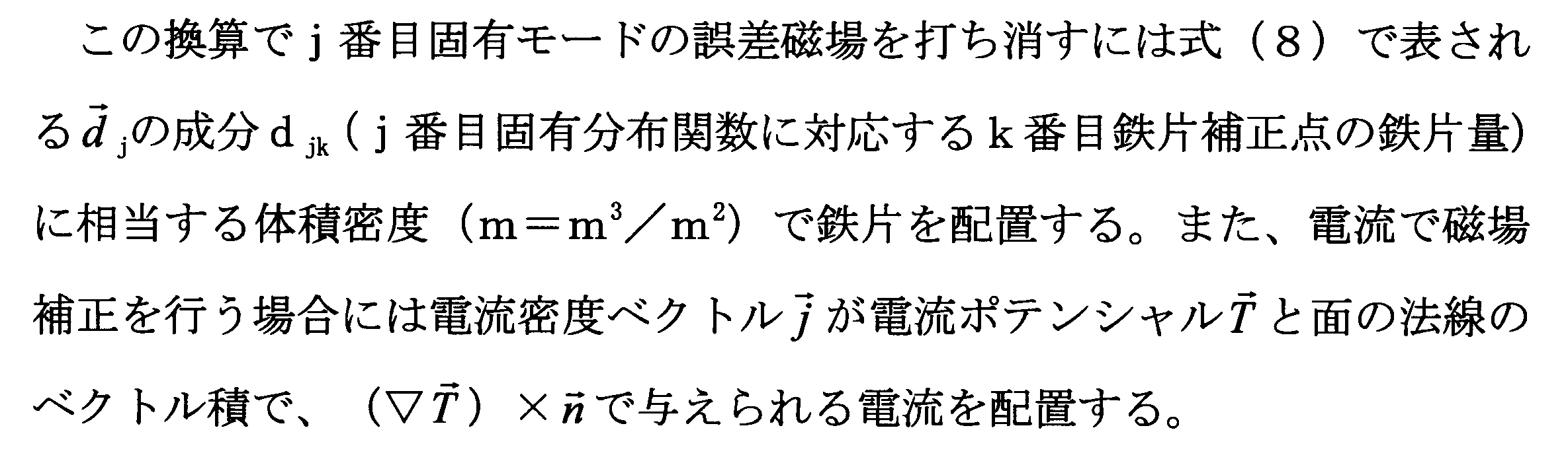
- FIG. 3A if there is a value in the contact 11 having the current potential T, it can be interpreted that the current 21 due to the current potential having the magnitude T is swirling between the contact points around it. . That is, this is equivalent to the situation where the current 1 flows in the current loop of the small coil 3 in FIG. This is equivalent to the situation on the right side where j m (A / m) is flowing through the surface of the magnetized iron piece 4.
- the current potential value T used to express the current distribution in DUCAS has a unit of [A] as a unit, which is the density [1 / m 2 ] of the magnetic moment [Am 2 ], A] can also be considered.
- the sufficiently magnetized iron piece 4 has a magnetic moment proportional to the volume because the magnetic moment is proportional to the product of the area surrounded by the magnetizing current and the length in the direction of the magnetic field. That is, at the time of adjusting the magnetic field, the current potential T is an amount proportional to the density of the iron piece 4 [weight g / m 2 or volume cc / cm 2 per unit area].
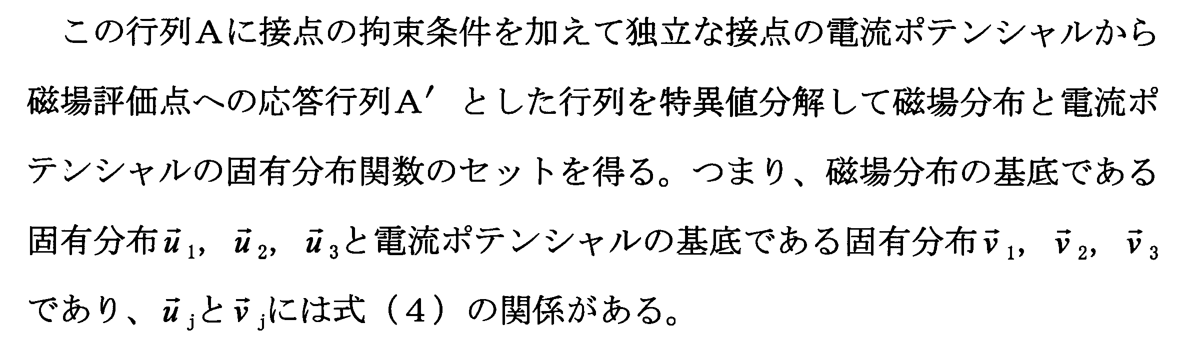
- the eigen distribution function and the singular value obtained by the singular value decomposition used in DUCAS are used instead of the spherical harmonic function of the conventional method.
- This provides a device that uses DUCAS to perform a support calculation for adjusting a magnetic field for a magnetic field generator and displays the arrangement of iron pieces or magnetic moments arranged for the adjustment. The operator can adjust the target magnetic field distribution by proceeding with the adjustment according to the display.
- an arbitrary magnetic field distribution can be set as the target magnetic field, but the following discussion will mainly be made on the assumption that the target magnetic field is a uniform magnetic field. However, whether the target magnetic field has a distribution does not affect the following discussion. It is simply to facilitate understanding of the discussion.
- FIG. 4 is a diagram showing a calculation system of the present embodiment. It consists of a current potential evaluation surface 13 and a set 14 of magnetic field measurement evaluation points.
- the current potential evaluation surface 13 may have a plurality of surfaces, but here, each of them will be discussed as one.
- Magnetic field evaluation points do not necessarily constitute a surface, but are shown here as points on the surface.
- the measurement point j has three-dimensional magnetic field components B xj , B yj , and B zj, but one point of measurement indicates the measurement magnetic field component by the measurement position and the unit vector p defined at that position. Even a single point in space may be three data in the present invention.
- FIG. 1 The general system for applying singular value decomposition is shown in FIG.
- ⁇ j is a singular value.
- the subscript j is a numerical value in the order in which the eigendistribution is numbered in the order of the singular values.
- One basis vector corresponding to each current potential distribution and magnetic field distribution corresponds to one number.
- the two basis vectors and one singular value related to this one number are collectively called one eigenmode.
- the order number j is the order of the eigenmode.
- the low-order eigenmode having a large singular value can generate a large magnetic field as can be understood from the fact that the magnetic field intensity per unit current potential distribution v j is ⁇ j u j .
- the magnetic field distribution is small.
- This property will be described later, it plays an important role in this magnetic field adjustment method.
- the distribution of eigenvectors obtained by singular value decomposition is used as the distribution function of equation (1).
- the relationship between current potential and iron piece density is described below.
- the iron piece can be replaced with a magnetic moment in consideration of the surface magnetizing current.
- the magnetization current j m (A / m) on the surface of the iron piece is as shown in equation (7).
- M magnetization (T). If the iron piece is in a saturated state, M is about 2.1T. Therefore, j m is about 1.7 ⁇ 10 6 A / m. Therefore the volume of the iron a cubic meter has a magnetic moment of about 1.7 ⁇ 10 6 Am 2 (170Acm 2 / 1cc). Since this value depends on the type of magnet, particularly the magnetic field strength, it needs to be examined individually. However, in the case of a magnet having a magnetic field strength exceeding about 1T, it can be considered that the iron piece is magnetized in a state close to saturation. At this time, the magnetic moment of iron is proportional to the volume.
- the eigendistribution function judged by the operator as being particularly necessary for correction is individually selected and corrected with the strength obtained from the inner product or the artificially determined strength. For example, when the error magnetic field distribution peaks overlap and a large error magnetic field is generated locally, the correction for artificially reducing the peak is corrected by selecting an appropriate eigen distribution function and the magnitude.
- the uniformity (reached uniformity) after correcting the current potential component of the selected eigendistribution function is obtained to determine whether the selection of the eigendistribution function is appropriate. If the arrival uniformity is not sufficient, the selection of the eigendistribution function is reviewed.
- the homogeneity indicates the ratio of the maximum and minimum magnetic field strengths among multiple measurement points in the magnetic field evaluation region, in other words, the difference between the maximum peak and the minimum peak of the error magnetic field to the average magnetic field. In MRI, discussions are usually on the order of 1 / million (ppm).
- Adjustment is performed by repeating the number of times from several times to several tens of times. This is because the accuracy of the adjusting mechanism is generally rough compared to the target magnetic field accuracy, and thus the adjustment mechanism is repeatedly operated to improve the magnetic field accuracy. For example, in the MRI magnetic field adjustment (shimming), it is necessary to adjust the magnetic field with an accuracy of 1 microT, but the error magnetic field before the adjustment is about several mT. When it is decided to adjust this at a stretch, the iron pieces to be arranged for the adjustment are required to manage the quantity with an accuracy smaller than 1/1000, but it is not easy to manage this accuracy in actual work.
- the amount of the magnetic field is controlled with an accuracy of about 1/10 or less in one adjustment, and the error magnetic field is reduced each time the number of times is adjusted, and the relative ratio to the final magnetic field accuracy is reduced. Sufficient final magnetic field accuracy can be obtained even with quantity control of 10 or less.
- the sum ⁇ is executed for the selected eigendistribution function. It can be easily calculated and predicted how the magnetic field distribution in the imaging region will be after this correction is executed.
- Equation (10) is obtained.
- the selection of the eigenmode of item (1) is made especially for correcting the error magnetic field for the low-order eigendistribution function.
- a low-order distribution function is selected as long as the magnetic field can be corrected with a relatively small amount of iron pieces. Even if it is only on the lower order side, tens to hundreds of eigendistribution functions are usually selected.
- By correcting the magnetic field according to the iron piece (current potential) arrangement of the eigendistribution function it is possible to correct the eigendistribution that has not been selected so as not to have a large influence and a new error magnetic field. This is particularly advantageous in that it does not disturb the higher order (numbered large numbered eigendistribution) that was not selected. That is, when the magnetic field adjustment is performed, the high-order eigen distribution not selected is not disturbed, and the work is not complicated.
- the low-order eigendistribution function selected in the singular value decomposition can be corrected with a small amount of iron pieces, but a large amount of iron is required to change the higher order.
- the reason why the higher order part is not disturbed is that, besides the fact that the distribution is orthogonal, a higher amount of iron pieces is required. That is, in the correction of the low-order distribution function in which a small amount of iron pieces is arranged, even if the arrangement is disturbed due to an error, the intensity of the high-order component does not change. In this sense as well, correction is performed by selecting from the low-order eigendistribution.
- the magnetic field that can be corrected is large in proportion to the singular value in the low order, the magnetic field adjustment, that is, shimming can be performed efficiently with a small amount of iron pieces.
- Item (2) does not correct eigen distribution function components that do not require correction. However, even if selected and included in the correction amount, the correction amount is small, so that the higher-order components are not disturbed as described above, so that no problem occurs.
- Item (3) adjusts the selection to adjust the iron piece arrangement amount and magnetic field distribution.
- the magnetic field is corrected using only the iron piece, it may be difficult to perform adjustment by the amount of the negative iron piece that removes the iron piece.
- the high-order distribution generates only a small magnetic field even if iron pieces are arranged. That is, a high-order component iron piece is arranged to make room for removing the iron piece during low-order correction.
- the uniformity is defined in the range from the positive peak to the negative peak value, there is a case where only the peak portion is concentrated and the display of the uniformity is deteriorated. In this case, an appropriate correction component is artificially added. This makes it easier to reach the target uniformity.
- Item (4) allows you to check whether the magnetic field can be adjusted with the target accuracy.
- the magnetic field is corrected for the selected eigendistribution function, it is necessary to finally reach the target uniformity if it is corrected repeatedly.
- this method it is possible to estimate how much uniformity can be obtained by the calculation method already described. Whether or not the selection of the eigendistribution function is changed according to this estimation, and if only a very uniform value can be obtained, it can be determined that there is a problem in production and that there is a problem in quality. Quality problems are likely to occur with higher-order components that are difficult to correct, but with the method of the present invention, components are separated by singular value decomposition, so problems that occur in higher-order eigenmodes can be easily found. it can.
- Item (5) is selection of how much the magnetic field strength to be made uniform is.
- the eigen distribution function is selected while changing the target magnetic field, the arrival uniformity and the amount of iron pieces are checked, and the target magnetic field with good uniformity and easy arrangement of the iron pieces is selected.
- the easy placement of the iron pieces does not simply mean that the amount is small, the necessary relatively low-order distribution function can be corrected sufficiently, and there is no region where the iron pieces cannot be arranged with the calculated negative iron amount Arrangement.
- Item (6) completes the magnetic field adjustment by repeating the work from the measurement to the iron piece arrangement.
- the eigendistribution function changes.
- the eigen distribution is initially selected up to the higher order, the magnetic field adjustment is performed, and the quantity is adjusted to be large, and the upper limit of the order is gradually lowered.
- the adjustment accuracy which is about 1/10 of the quantity, is also improved.
- a target magnetic field uniformity can be obtained with a small correction amount while predicting the adjusted magnetic field. It is necessary to perform shimming work repeatedly. In the middle of repetitive work, especially when high-order distribution shimming is performed, the error magnetic field component corresponding to the low-order distribution function may increase and the uniformity may appear to deteriorate.
- Example 1 will be described. As an embodiment 1, application of an open MRI apparatus having a vertical magnetic field to magnetic field adjustment (shimming) will be described.
- FIG. 5 shows a system for shimming (magnetic field adjustment) the magnetic field generated by the magnet of the MRI apparatus.
- FIG. 1 shows a shimming flow for adjusting the magnetic field distribution in this embodiment. It is an Example applied to the magnetic field adjustment of the imaging field of a perpendicular magnetic field type
- the surface of the magnetic field adjustment mechanism (the shim tray 5) is above and below the imaging region with the strength of the magnetic field component perpendicular to the ground, and the iron piece 4 is placed on the surface.
- FIG. 6 shows an example of mesh generation when the present embodiment is applied to shimming of an MRI apparatus.
- the spherical surface is a set 14 of magnetic field measurement evaluation points, and hundreds of magnetic field measurement points are arranged.
- the upper and lower disk surfaces of the sphere are the calculation model of the surface on which the iron piece 4 is arranged when performing shimming, that is, the current potential evaluation surface 13.
- a finite element calculation system composed of triangular elements having contacts on this surface is constructed.
- Step 1 includes a singular value decomposition calculation step 32S for calculating the preliminary calculation portion 1B in the broken line prior to the shimming operation, and includes a calculation mesh generation step 31S, and an eigen distribution function and a singular value as a result of the singular value decomposition.
- Step 33S is included.
- This portion is a preliminary calculation portion 1B including a singular value decomposition of the response matrix A from the contact corresponding to several thousand current potential values to the magnetic field measurement points of about several hundred points in the imaging region. Need time. For this reason, the eigendistribution function for shimming is calculated with a calculation system adapted to the magnet system, thereby shortening the calculation time during the shimming operation.
- the data calculated in advance is stored in the storage area of the computer in the storing step 33S, and is read out when necessary (single value decomposition result reading step 16S).
- the computer there are several or more eigendistribution functions that are the basis vectors of the magnetic field distribution, the same number of basis vectors that are the distribution functions of the current surface, and the same number of singular values that are conversion information of the magnitudes of both. Are stored in combination.
- the magnetic field adjustment (shimming) start step 11S is started. Work is performed according to the flow of FIG. After the magnetic field measurement step 12S and the magnetic field distribution data storage step 13S and the magnetic field data read step 14S, it is determined whether the uniformity is good in the magnetic field uniformity determination step 15S. If the uniformity is sufficient, shimming is not necessary, and the magnetic field adjustment end step 40S is performed. This may be the case when the device used with sufficient uniformity is de-energized after degaussing at the time of maintenance, etc., but the new magnet has a uniformity of several hundred to 1000 ppm due to manufacturing errors, and the magnetic field It is determined that adjustment (shimming) is necessary.
- step 19S for determining the validity of the eigenmode selection.
- the calculation result of step 18S is displayed to determine the validity of the eigenmode selection.
- FIG. 7 is a spectrum in which the strength of the eigen distribution of the magnetic field included in the error magnetic field obtained by the equation shown in equation (5) is shown on the vertical axis and the order of the eigen mode is shown on the horizontal axis. To do.
- the vertical axis shows the logarithmic scale.
- FIG. 7 also shows the eigenmode selection range and reachable uniformity.
- FIG. 8 shows a display example of the iron piece arrangement amount for shimming work together with current potential contour lines.
- the calculation contents shown in this example are the system shown in FIGS. 5 and 6, but the target is a uniform magnetic field where the magnetic field evaluation point is on a surface having a diameter of 40 cm and the error magnetic field of this surface is 20 ppm or less.
- the eigen distribution function to be corrected is selected.
- x corresponds to each eigenmode, but the one surrounded by ⁇ is the selected eigenmode 15.
- Those not enclosed in circles are non-selected eigenmodes 16. This selection is made by the method already described.
- the reachable uniformity can be calculated and predicted by subtracting the error magnetic field component from the measurement error magnetic field.
- the reachable uniformity 17 is shown in a portion surrounded by an ellipse at the top.
- FIG. 7A is before shimming and FIG. 7B is after shimming. It is 726 ppm in this example before shimming, and it can be seen that the error magnetic field component in the low-order mode is large in the spectrum diagram.
- A is an eigenmode selected as an error magnetic field component having an order of 80 or less and a strength almost equal to or greater than the lower limit of measurement accuracy. In this example, if the selected eigenmode is corrected, it is predicted to be 15.25 ppm.
- a line 22 indicating the upper limit of the eigenmode selection and a line 23 indicating the lower limit of the eigenmode selection are displayed on the spectrum diagram of FIG. 7 to select the eigenmode.
- the selection of the eigendistribution function is reconsidered. Adjusting the number of unique distribution functions, namely to adjust the lower limit of the specific distribution function selection number on the lower limit or eigenmode intensity C j of. There are also options such as adjusting the correction ratio of the individually selected eigendistribution function.
- the other display in step 19S is used for checking whether or not shimming is possible in the iron piece arrangement amount instruction diagram of FIG.
- the circle in the figure shows the shim tray 5 shown in FIG. Although there are two upper and lower sheets, this is the lower shim tray.
- the cells 7 in the figure are sections arranged on the shim tray 5, and each is assigned an address. In FIG. 7, addresses are designated by A, B, C --- in the left-right direction and 1, 2, 3, ---- in the up-down direction.
- the numerical value in the mesh 7 indicates the iron volume 18 arranged in the mesh.
- the unit is 0.1 cc.
- the grid has a structure in which iron pieces of about 5 cc can be sufficiently arranged, and the amount of display is sufficiently small and can be arranged. Since the amount of iron pieces to be handled is gradually reduced during the repeated adjustment, it is displayed in units as small as 1/10, 1/100, 1/1000 of the original.
- FIG. 8 shows a contour line 19 of the current potential on the current potential evaluation surface 13 obtained by modeling the shim tray 5 in addition to the grid piece 7 and the iron piece amount 10 of the grid.
- the current potential contour line 19 is considered as a coil shape, the error magnetic field can be corrected by the coil having this shape. This is described in the previously published paper mentioned above.
- the contour display in the present invention has another advantage.
- the distribution function obtained by singular value decomposition requires an arrangement of iron pieces or magnetic moment with a spread on the surface. However, the most arrangement (or removal) is required in the vicinity of the peak 8 of the contour line and the valley 9 of the contour line. Using these two properties, the arrangement position of the iron piece for adjusting the magnetic field is flexibly considered.
- the amount of iron pieces of the current potential contour line 19 closed with the same sign around the contour peak is added and placed near (removed from) the peak 8 position of the contour line. Also, if the vicinity cannot be placed due to, for example, a shim tray fixing support, the same amount of placement may be placed (removed) in other parts within the closed contour region. .
- FIG. 9 shows a conversion concept from the contact potential value to the magnetic moment and the iron piece amount in the magnetic field adjustment calculation of this embodiment.
- the current potential can be interpreted as indicating the magnetic moment per unit area. Therefore, in order to obtain the iron piece amount in a certain area, the current potential T is integrated in the area to obtain a magnetic moment necessary for the area, and converted to the iron piece amount as described above.
- FIG. 9 schematically shows the relationship between the mesh 7 shown in FIG. 8 and the contacts. A point indicated by ⁇ is a contact point.
- the product of the contact point and the area corresponding to the contact point is added to obtain the magnetic moment in the mesh 7 as in the equation in the figure.
- the area corresponding to the contact may be 1/3 of the element to which the contact belongs (in the case of ⁇ element).
- the size of the mesh 7 is required to be fine enough to have the resolution of the iron amount distribution shown in FIG.
- the contour line distribution is confirmed near the upper limit of the order of the eigenmode necessary for obtaining the uniformity, and is assumed to be smaller than the size of the peak or valley portion. On the other hand, it takes time and effort to make a fine mesh. In FIG. 8, it is approximately the same as the minimum size of the peak 8 of the contour line and the valley 9 of the contour line. Because of the same degree, there are some areas where fine contour lines do not have sufficient resolution with only the mesh 7. In this case, the iron piece is arranged by adjusting the position with reference to the peak and valley positions of the contour lines.
- the size of the finite element is determined by the number of contacts in the grid. As already described, the accuracy of the iron piece arrangement amount may be about 1/10, and the uniformity is increased repeatedly. If the number of contacts is about 5 or more, even if a slight error occurs in the corresponding area, it is considered that the accuracy is sufficient. In the example of FIG. 8, one side has about 1500 contacts. As shown in FIG. 6, the upper and lower shim trays are considered as current evaluation surfaces, and the total of two sheets is considered to be about 3000 contacts or more.
- the iron piece arrangement work step 22S was performed.
- the basis for this prediction is that the reachable uniformity 17 is sufficiently better than the target value and the amount of iron pieces can be arranged.
- the process returns to the eigenmode selection and target magnetic field determination step 17S again. However, if it is determined that the magnetic field adjustment is not possible in step 21S for determining whether the target magnetic field can be adjusted even if various conditions are changed, the magnet is defective and the repair / adjustment step 41S is entered.
- Fig. 7 (b) shows the spectrum at the end of shimming. Shimming can be achieved up to a uniformity of 17 ppm. It can be said that the uniformity was predicted with good accuracy and with a uniform uniformity compared with the 15 ppm level predicted at the beginning. Until the spectrum uniformity shown in FIG. 7A is reached, the repetitive operation is performed as shown in the flow of FIG. The necessity of this repetition has already been described, but will be described later with an example.
- step 21S The possibility of adjusting the magnetic field is determined in step 21S, which will be described below. Even after returning to step 17S via step 21S and reexamining eigenmode selection, sufficient uniformity may not be obtained with an appropriate correction amount (shim iron piece amount). In other words, this is a case where the manufacturing accuracy of the magnet is insufficient, the magnetic field is poor, and a large amount of iron pieces is required to obtain the target uniformity, which is actually impossible.
- a magnetic field defect can be detected without adjusting the magnetic field. If it is defective, appropriate correction is performed, but the problem location can be estimated from the correction amount distribution. Further, if it cannot be repaired, it is possible to determine that the product is defective, and the present invention also includes the advantage that determination can be made without using manual labor by repeatedly adjusting the magnetic field.
- the iron piece distribution calculation result necessary for correction is output by paper printing or enlarged display by project, and the shimming iron pieces are arranged according to the distribution.
- Do work There is an error in the amount and position of the iron piece to be placed in the shimming operation, and there is an error in the iron piece conversion from the current potential because the degree of iron piece magnetization depends on the material properties of the iron piece and the magnetic field distribution in the magnet. To do. For this reason, the reachable uniformity cannot be reached in one operation. Therefore, the work is repeated as shown in FIG. 1 to bring the magnetic field closer to uniform.
- Example 2 will be described. Although it has already been described that it can be used for quality inspection after production, this method can be used for magnet design with the same judgment.
- the flow in this case is shown in FIG.
- the magnetic field adjustment is performed in calculation, and it is applied to the magnetomotive force arrangement design by confirming that the target magnetic field accuracy can be achieved.
- step 52S that assumes the magnetomotive force arrangement is performed.
- a magnetic field calculation step 53S is performed based on this magnetomotive force arrangement.
- the singular value decomposition is executed based on the arrangement of the shimming trays from the magnetomotive force arrangement and the result is stored.
- This preliminary calculation portion 1B is the same as that in the first embodiment.
- the portion 1B is executed based on the magnetomotive force arrangement assumption step 52S only when it is determined that the shim tray needs to be changed in the magnetomotive force arrangement improvement determination step 56S.
- This preliminary calculation unit 1B is the same as in FIG.
- step 56S it is determined whether or not the existing singular value decomposition data can be used, and depending on the result, only the step 16S of reading out the data set of the singular value decomposition results is set.
- Step 14S for reading out the magnetic field calculation result and step 15S for determining the magnetic field uniformity are executed. If the uniformity is already good, the magnetomotive force arrangement candidate proposal step 56S for the MRI magnet is performed. In general, it is determined from the magnetic field distribution whether the uniformity is improved by shimming using the technique of the present invention already described. When the uniformity is not sufficiently improved by shimming, or when it is determined that shimming is impossible due to an excessive amount of iron pieces necessary for shimming, the process returns to the magnetomotive force arrangement assumption step 52S again.
- This determination portion 3B is the same as steps 17 to 21S in FIG.
- the magnetic field adjustment calculation part 3B is also the same as 3B in FIG.
- step 55S whether or not to improve by correcting the magnetomotive force arrangement in step 55S is examined with reference to the amount of iron pieces necessary for shimming and with reference to the structural design of the entire magnet. If the magnetomotive force arrangement is not reexamined, the candidate MRI magnet magnetomotive force arrangement candidate plan 56S is obtained. When correcting the magnetomotive force arrangement, the process returns to the magnetomotive force arrangement assumption step 52S again. In the case of reexamining the magnetomotive force arrangement, for example, the empirical magnetic field of the superconducting coil is excessive, or the support structure has a difficult electromagnetic force.
- the shimming of the present invention is virtually performed in calculation to obtain a magnetomotive force arrangement candidate.
- the entire design of the magnetomotive force amount, electromagnetic force, and stress is performed, and the feasibility of the magnet is further determined. If it is found that the feasibility is difficult, start by assuming the magnetomotive force arrangement again.
- FIG. 1 as a magnetic field adjusting means, a method using a magnetic moment of the magnetized iron piece 4 is described as iron piece arrangement work step 22S.
- the magnetized iron piece is equivalent to the current by the small coil 3. Therefore, it is also possible to arrange the small coils in the grid shape of FIG. 8 and adjust the current 1 according to the magnetic moment distribution calculated by this method as an alternative to the iron piece arrangement work step 22S.
- magnetic field adjustment requiring a negative amount may be required.
- it can be handled by changing the polarity of the current, and when using a permanent magnet, by changing the direction, the magnetization of the iron piece is determined by the surrounding magnetic field environment, The polarity cannot be changed.
- the negative amount in this case is considered as follows. When the higher order part is selected, the negative part is not arranged.
- the uneven vibration spatial wavelength of the error magnetic field is about 1 ⁇ 2 times, and the natural mode order of the error magnetic field component that is not canceled by not arranging the negative mass is about Moving to the higher order side of the double order, the singular value decreases, the magnetic field strength also weakens, and can be ignored for magnetic field adjustment.
- the requirement for a negative amount can usually be adjusted by a method of reducing the amount of iron pieces already arranged by magnetic field adjustment up to the higher order. .
- the iron amount is already zero in the mesh, it is removed from the vicinity. Neighboring is from a region of closed lines of contour lines. If there is still no iron piece to be taken, the specific natural mode is artificially removed from the size necessary for correction so that the negative amount is eliminated.
- the magnetic field adjustment calculation part 3B is made especially of software, so that when performing magnetic field adjustment, the stored data of the singular value decomposition result and the magnetic field adjustment support tool with good mobility. It becomes.
- Examples 1 and 2 an example in which iron pieces are arranged with an amount that generates a necessary magnetic moment has been shown.
- a negative amount is required as the amount of iron to be arranged, In some cases, the amount of iron that can be removed is insufficient or zero. If there is a case where sufficient uniformity does not occur even if it is handled as described above, the permanent magnet 4P or the current loop 4C is used instead of iron. There is no problem even if these are applied to a positive iron amount, but it is desirable to use an iron piece that can be shimmed at low cost if it can be dealt with by magnetization of iron.
- a state in the mesh frame in actual shimming will be described as an example. As shown in FIG. 11, even in the case of Example 1 and Example 2, it is assumed that some iron pieces 4 having different volumes are arranged in the actual mesh. The magnitude of the magnetic moment differs between Mf1 to Mf4. The required magnetic moment shown in FIG. 9 is as shown in equation (13) for each Mfi. The volume of the iron in the frame is adjusted with a combination of iron pieces having different volumes so that the magnetic moment obtained from Equation (13) can be generated.
- Ti is the current potential value (A) of the contact i in the frame
- Si is the area attached to the contact. Since the contacts are attached to a plurality of elements, there is no problem with the triangular element shown here assuming that 1/3 of each element belongs to each contact.
- the conversion method of the volume of the iron piece and the magnetic moment has already been discussed in FIG. 3, but the magnetic moment of the iron piece saturated with reference to Equation 9 can be converted at about 170 Acm 2 / cc per cc.
- the magnetic moment required for the grid is converted into the volume of the iron piece, and the required volume is placed in the grid.
- the permanent magnet 4P When the permanent magnet 4P is used, the only difference from the iron piece 4 is the magnetic moment conversion method.
- the permanent magnet 4P can arrange the magnetic moment Mp even in the direction opposite to the surrounding magnetic field as shown in FIG. That is, a negative iron piece amount can be arranged. Therefore, the sign of the physical quantity can be arranged in the direction of the magnetic field or in the opposite direction according to the sign of the volume that requires the direction of Mp.
- the magnetic moment, volume, and conversion are read from the MH curve. That is, the magnetization M is read from the MH curve when the permanent magnet is arranged in the reverse direction from the magnetic field H at the arrangement position. If the magnetization is read, it can be converted by the same method as the already described magnetization of iron.
- the required permanent magnet volume is approximately determined by equation (14). In the equation (14), the magnetization M may be negative.
- the current is adjusted from the power supply 10 in consideration of the sign so that this magnetic moment becomes the same as the required magnetic moment.
- the magnetic moment generation method and materials used for actual shimming are shown in FIGS. 11, 12, and 13, but other magnetic materials such as nickel and cobalt are also conceivable in addition to iron.
- the magnetization curve is examined as described for the permanent magnet, the converted magnetic moment is obtained, the necessary volume is obtained, and the volume is arranged in the grid as in FIGS.
- magnetization cannot be obtained from the magnetization curve For example, there is a case where a magnetic material for shimming occurs when the magnetic field is different from the base magnetic field. In this case, it is desirable to measure the degree of magnetization of the magnetic material.
- the surrounding magnetic field is measured before and after placing a magnetic piece whose magnetization is actually unknown, and compared with the change in the magnetic field due to the placement when the magnetization is known. Or, it will be compared with the calculated magnetic field change. Further, if the magnetization curve is only of a known material, a detailed nonlinear magnetic field calculation is performed and used as a calculated value of magnetization 4 of the iron piece arranged from the calculation result.
- the final arrival uniformity is predicted, the quality of the magnet is confirmed, the error is automatically corrected, and the measurement / correction iron arrangement calculation / arrangement is repeated to ensure Magnetic field adjustment can be performed. It can also be used for magnetomotive force arrangement design of magnets that require high magnetic field accuracy.
- the present invention relates to a magnetic field distribution in a desired magnetic field intensity distribution in a magnet apparatus that generates a magnetic field by arranging a coil and a magnetic material such as iron, such as a nuclear magnetic resonance tomography apparatus (MRI) used for medical diagnosis.
- a nuclear magnetic resonance application apparatus such as MRI provides a method and apparatus for uniformizing with extremely high accuracy in a measurement region.
- the error magnetic field is corrected by arranging the iron pieces, and the error magnetic field distribution and the iron piece arrangement distribution are corrected to a uniform magnetic field distribution by a combination of the respective orthogonal bases in an operation called shimming for uniforming the magnetic field strength.
Landscapes
- Physics & Mathematics (AREA)
- Condensed Matter Physics & Semiconductors (AREA)
- General Physics & Mathematics (AREA)
- Magnetic Resonance Imaging Apparatus (AREA)
Abstract
Description
(1)時間的に定常で空間的にも一定な磁場で、通常0.1から数テスラ以上の強さである、撮像を行う空間(通常直径で30-40cmの球もしくは楕円体の空間)ないで数ppm程度の変動範囲である。
(2)1秒程度以下の時定数で変化して、空間的に傾斜した磁場。
(3)核磁気共鳴に対応した周波数(数MHz以上)の高周波の電磁波によるもの。
このうち(1)の磁場は時間的に一定で、かつ空間的にも人体の断層撮影を行う領域では極めて高精度に均一性が磁場強度に要求される。高精度とは、たとえば40cm直径の撮像空間FOV(Field of View)で、±1.5ppmのように百万分の1のオーダの精度が要求される。このようにきわめて高精度な均一性が要求される磁場分布は、磁石を製作・励磁の後に磁場を精度よく調整する必要がある。一般に製作誤差による誤差磁場は均一磁場に要求される許容誤差磁場に比べて1000倍以上大きい。製作後の据え付け時に要求される磁場調整(シミング)は数100ppmから数ppmへの誤差磁場の低減を行うことになり、きわめて高精度な磁場調整装置およびその手法が要求される。
(1)詳細な磁場計算を行うために多くの計算時間が必要である。
(2)ここの鉄片や電流の設置や変化に高精度の磁場に対応した精度を要求される。
(3)誤ったシミング作業を行った場合に、誤った箇所の特定が難しく回復に手間がかかる。



















(a)製作完了時の品質管理
(b)コイルや磁性体配置の設計時に、起磁力配置の設計の妥当性,配置の再検討要否の検討に利用できる。
項目(1)の固有モードの選択は特に低次側の固有分布関数について誤差磁場を補正するために選択する。比較的少量の鉄片で磁場が補正できる範囲で低次の分布関数を選択する。低次側のみと言っても通常数十から数百の個数の固有分布関数を選択する。固有分布関数の鉄片(電流ポテンシャル)配置に従って磁場を補正することで、選択しなかった固有分布に対しては大きな影響、新たな誤差磁場を与えないように、補正できる。これは、特に、選択しなかった高次(番号付けした大きな番号の固有分布)を乱さないという点で利点がある。つまり磁場調整を行っているときに、選択しなかった高次固有分布が乱れて作業が繁雑になることはない。

永久磁石4Pを用いる場合、鉄片4と異なる点は、磁気モーメントの換算法のみである。永久磁石4Pは図12のように周囲の磁場と逆方向でも、磁気モーメントMpを配置できる。つまり負の鉄片物量が配置できる。従って、Mpの方向を必要とする体積の符号に合わせて、磁場の方向もしくは反対方向で、物量の正負を配置できる。磁気モーメントと体積と換算は、M-H曲線から読みとる。つまり配置する位置での磁界Hから,永久磁石を逆方向に配置する場合にはM-H曲線から、磁化Mを読みとる。磁化が読みとれば既に説明した鉄の磁化と同じ方法で換算できる。必要な永久磁石体積おおよそ式(14)で求められる。式(14)では磁化Mが負になる場合もある。


実際のシミングに用いる磁気モーメントの発生方法とその材料について図11,12,13に示したが、このほかにも、鉄でなく、ニッケルやコバルトなどの他の磁性体も考えられる。この場合には、永久磁石で述べたように磁化曲線を調べて、その換算磁気モーメントを求め、その上で必要な体積を求め、図11、12と同様に升目内に配置していく。
磁化曲線で磁化が求められない場合も存在する。例えばシミング用の磁性体が、磁場が基の磁場とは異なる場合が発生するケースである。この場合には磁性体の磁化の程度を計測することが望ましい。例えば、実際に磁化が不明な磁性体片を配置する前後で、周囲の磁場を計測し、磁化が既知の場合の配置による磁場変化と比較する。もしくは計算上の磁場変化と比較することになる。また、磁化曲線が既知の材料のみで有れば、詳細な非線形磁場計算を行い、その計算結果から配置した鉄片の磁化4計算値として利用する。
2 磁化電流
3 小コイル
4 鉄片
4P 永久磁石
4C 電流ループ
5 シムトレイ
6 磁場計測評価領域
7 升目
8 等高線のピーク
9 等高線の谷
10 直流電源
11 接点
12 有限要素
13 電流ポテンシャル評価面
14 磁場計測評価点の集合
15 選択した固有モード
16 非選択の固有モード
17 到達可能均一度
18 升目に配置する鉄体積
19 電流ポテンシャル等高線
21 電流ポテンシャルによる電流
22 固有モード選択の次数上限を示す線
23 固有モード選択で強さ下限を示す線
1B 予備計算部分
2B 磁場計測部分
3B 磁場調整計算部分
11S 磁場調整開始ステップ
12S 磁場計測ステップ
13S 計測磁場保存ステップ
14S 磁場データ読み出しステップ
15S 均一度判断ステップ
16S 特異値分解結果読み出しステップ
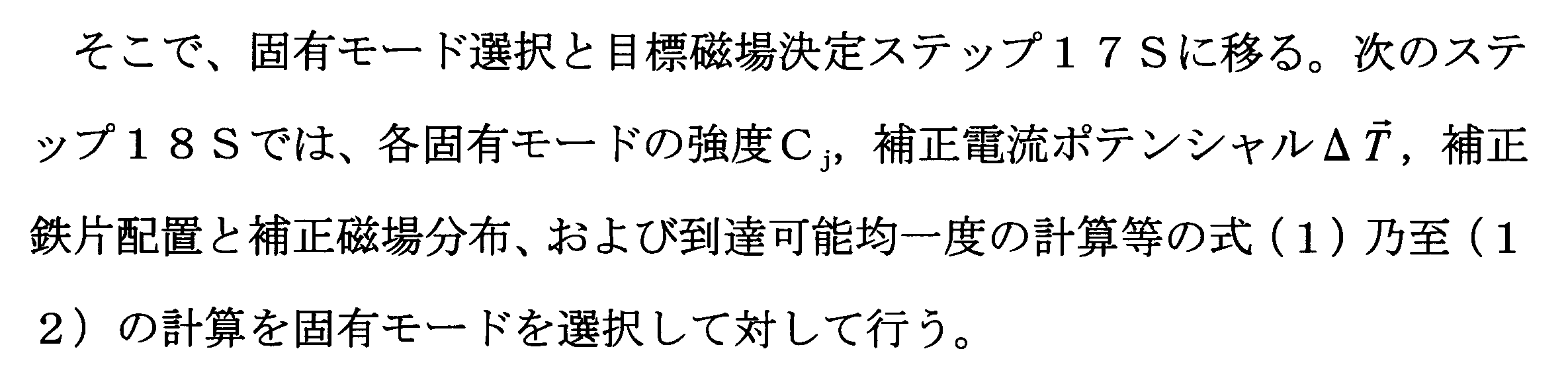
17S 固有モード選択と目標磁場決定ステップ
18S 固有モード強度,補正電流ポテンシャル,鉄片量,補正磁場分布および到達可能均一度計算ステップ
19S スペクトル,到達可能均一度および鉄片配置量計算ステップ
20S シミング可否の判断ステップ
21S 品質良否判断ステップ
22S 鉄片配置作業ステップ
31S 計算メッシュ生成ステップ
32S 特異値分解計算ステップ
33S 特異値分解結果保存ステップ
40S 磁場調整終了ステップ
41S 修理・調整ステップ
51S 起磁力配置検討開始ステップ
52S 起磁力配置仮定ステップ
53S 磁場計算ステップ
54S 磁場計算結果保存ステップ
55S シムトレイ変更要否判断ステップ
56S 起磁力配置改善判断ステップ
Claims (16)
- 磁場発生装置に目標の磁場分布が与えられた領域があり、その領域の磁場分布の誤差磁場成分を低減し、目標に磁場分布に近づける磁場調整法において、
調整手段として、電流ループ、および受動的に磁化する鉄片などの磁性体や外部磁場に依存しない永久磁石を配置する曲面もしくは平面状の磁場調整機構を持ち、
所定数の点において磁場計測を行い、目標磁場との差である誤差磁場を算出し、その誤差を近似的に補正できる磁場調整機構面上の電流ポテンシャル分布を求め、その電流ポテンシャル分布を磁気モーメントに換算し、その磁気モーメントに相当するループ電流、永久磁石もしくは磁性体片を配置する磁場調整作業を特徴とする磁場調整法。 - 請求の範囲第1項の磁場調整法において、特異値分解により得た基底である固有分布関数の中から分布関数を選択し、その組み合わせで近似的に誤差磁場を補正する電流ポテンシャルの分布を表現することを特徴とする磁場調整法。
- 請求の範囲第2項の磁場調整法で、近似的に補正する電流ポテンシャルから目標磁場を与えた領域のおよび磁場計測点の補正磁場量を計算し、磁場調整作業後の目標磁場からの残留誤差磁場を求め、固有分布関数の選択の妥当性を確認すると共に、目標の残留誤差磁場以内となる選択を行うことを特徴とする磁場調整法。
- 請求の範囲第1項の磁場調整法において、電流ポテンシャルを磁気モーメントに比例する量として、鉄片量密度に換算し、その換算した分布に従って鉄片または永久磁石を配置することを特徴とする磁場調整法。
- 請求の範囲第1項の磁場調整法において、誤差磁場の補正に必要な電流ポテンシャル分布を求める固有分布関数の選択を、特異値の大きさの順に並べて番号付けした番号(次数)と、誤差磁場に含まれる固有分布の強さの相関図(スペクトル図)上で選択することを特徴とする磁場調整法。
- 請求の範囲第1項の磁場調整法において、電流ポテンシャル、または、磁気モーメントの大きさもしくは鉄片量や永久磁石量について、密度分布を鉄片を配置する磁場調整機構面上に等高線を含む表示を行い、その表示に従って鉄片を配置することを特徴とする磁場調整法。
- 請求の範囲第6項の磁場調整法において、等高線とともに鉄片を配置する面を多角形で分割し、分割した領域毎に、磁気モーメントの大きさもしくは鉄片量や永久磁石量を、面積積分値で、等高線と共に、もしくは等高線無しで示すことを特徴とする磁場調整法。
- 請求の範囲第6項の磁場調整法において、等高線で示した山もしくは盆地部をまとめて積算し、その量を山もしくは盆地部内の一カ所もしくは複数箇所に分散して配置することを特徴とする磁場調整法。
- 請求の範囲第1項の磁場調整方法で、磁場計測から磁気モーメントの大きさもしくは鉄片量や永久磁石量の配置までの計算と作業を繰り返し実行することを特徴とする磁場調整法。
- 請求の範囲第9項の磁場調整法で、繰り返し計算と作業で、誤差磁場の大きさと共に、特異値分解で得た磁場分布を表す基底である固有分布関数について、個々の強度の大きさを調べて、磁場調整の進展を把握することを特徴とする磁場調整法。
- 請求の範囲第3項の残留誤差磁場の代表値、たとえば最小最大値の差を目標もしくは計測磁場の平均磁場強度で割った値を、請求の範囲第5項の相関図、または請求の範囲第6項、第7項、もしくは第8項の磁場補正作業で配置する磁性体の量,永久磁石の量もしくは電流ループの大きさと共に、表示することを特徴とする磁場調整法。
- 磁場発生用のコイルや磁性体の起磁力源を含む電磁石の請求の範囲第3項の磁場調整法で、目標の誤差磁場以下とする条件での、請求の範囲第6項または第7項の磁気モーメントの大きさ、鉄片量または永久磁石量の配置が可能であることで、磁場調整が正常に実行できることを、磁場調整作業開始時に判断できることを特徴とする磁石品質把握法。
- 磁場発生用のコイルや磁性体の起磁力源を含む電磁石の設計において、目標磁場分布が与えられ、起磁力配置から磁場分布を計算し、請求の範囲第12項の磁場計測値を代替する磁場計算値を入力し、配置した起磁力源配置の妥当性を確認し、妥当で無ければ、磁場調整が可能となるまで起磁力配置を変更して、磁場調整が可能な起磁力配置を求めることを特徴と磁石起磁力配置設計法。
- 請求の範囲第1項乃至第11項のうちの1項に記載する磁場調整法を内蔵する装置。
- 請求の範囲第12項に記載する磁石品質把握法を内蔵する装置。
- 請求の範囲第13項に記載する磁石起磁力配置設計法を内蔵する装置。
Priority Applications (3)
| Application Number | Priority Date | Filing Date | Title |
|---|---|---|---|
| CN200980116540.3A CN102046083B (zh) | 2008-05-09 | 2009-05-08 | Mri装置用磁场调整 |
| JP2010511090A JP4902787B2 (ja) | 2008-05-09 | 2009-05-08 | Mri装置用磁場調整 |
| US12/991,495 US8947089B2 (en) | 2008-05-09 | 2009-05-08 | Magnetic field shimming adjustment: reducing magnetic distribution errors by obtaining current potential distributions of MRI apparatus |
Applications Claiming Priority (2)
| Application Number | Priority Date | Filing Date | Title |
|---|---|---|---|
| JP2008122843 | 2008-05-09 | ||
| JP2008-122843 | 2008-05-09 |
Publications (1)
| Publication Number | Publication Date |
|---|---|
| WO2009136643A1 true WO2009136643A1 (ja) | 2009-11-12 |
Family
ID=41264697
Family Applications (1)
| Application Number | Title | Priority Date | Filing Date |
|---|---|---|---|
| PCT/JP2009/058713 Ceased WO2009136643A1 (ja) | 2008-05-09 | 2009-05-08 | Mri装置用磁場調整 |
Country Status (4)
| Country | Link |
|---|---|
| US (1) | US8947089B2 (ja) |
| JP (2) | JP4902787B2 (ja) |
| CN (1) | CN102046083B (ja) |
| WO (1) | WO2009136643A1 (ja) |
Cited By (7)
| Publication number | Priority date | Publication date | Assignee | Title |
|---|---|---|---|---|
| WO2011065357A1 (ja) * | 2009-11-24 | 2011-06-03 | 株式会社日立製作所 | Mri装置用磁場調整方法 |
| JP5122029B1 (ja) * | 2012-03-01 | 2013-01-16 | 三菱電機株式会社 | 超電導マグネットの調整方法 |
| JP2013059488A (ja) * | 2011-09-13 | 2013-04-04 | Hitachi Medical Corp | 磁場調整方法及び磁場調整装置 |
| JP2015108614A (ja) * | 2013-10-16 | 2015-06-11 | ブルーカー バイオシュピン アー・ゲー | 次元数が低減されたパラメータ空間において最適化により目標磁場を決定することを含むシミング手順 |
| WO2016136465A1 (ja) * | 2015-02-25 | 2016-09-01 | 株式会社日立製作所 | 磁気共鳴イメージング装置、静磁場均一度調整方法、プログラム及び計算機 |
| JP2018029628A (ja) * | 2016-08-22 | 2018-03-01 | 株式会社日立製作所 | 磁気共鳴イメージング装置のシミング方法、磁気共鳴イメージング装置及びシールドルーム |
| JP2018196776A (ja) * | 2015-02-20 | 2018-12-13 | 株式会社日立製作所 | 磁場調整方法 |
Families Citing this family (17)
| Publication number | Priority date | Publication date | Assignee | Title |
|---|---|---|---|---|
| JP5060384B2 (ja) * | 2008-05-09 | 2012-10-31 | 株式会社日立製作所 | 磁場均一度調整用ソフトウェア、磁場均一度調整方法、磁石装置及び磁気共鳴撮像装置 |
| JP4902787B2 (ja) * | 2008-05-09 | 2012-03-21 | 株式会社日立製作所 | Mri装置用磁場調整 |
| BR112012013588B1 (pt) * | 2009-12-02 | 2021-01-26 | Nanalysis Corp. | método para homogeneizar um campo magnético, detector para detectar a ressonância magnética e painel para homogeneizar um campo magnético |
| DE102011087485B3 (de) | 2011-11-30 | 2013-05-29 | Siemens Aktiengesellschaft | Magnetresonanztomographie-Anlage, Verfahren zum Ausgleichen einer Feldinhomogenität in der Anlage und Shimspulenanordnung |
| JP5802163B2 (ja) * | 2012-03-29 | 2015-10-28 | 株式会社日立メディコ | 磁場均一度調整方法、磁石装置及び磁気共鳴撮像装置 |
| JP2014004169A (ja) * | 2012-06-25 | 2014-01-16 | Hitachi Medical Corp | 磁場調整方法、磁場発生装置、磁気共鳴イメージング装置及び磁場調整装置 |
| JP6001784B2 (ja) * | 2013-07-09 | 2016-10-05 | 株式会社日立製作所 | 磁場調整支援装置、磁場調整支援方法、mri装置および磁石装置 |
| CN107205689B (zh) * | 2015-02-20 | 2020-04-24 | 株式会社日立制作所 | 磁场均匀度调整方法以及磁场均匀度调整装置 |
| WO2016132831A1 (ja) * | 2015-02-20 | 2016-08-25 | 株式会社日立製作所 | 磁場調整用磁気モーメント配置算出方法、磁場調整装置およびプログラム |
| JP6392141B2 (ja) * | 2015-02-20 | 2018-09-19 | 株式会社日立製作所 | 磁場均一度調整方法、磁場均一度調整プログラムおよび磁場均一度調整装置 |
| WO2016133204A1 (ja) * | 2015-02-20 | 2016-08-25 | 株式会社日立製作所 | 磁場調整支援システムおよび磁場調整方法 |
| JP6643110B2 (ja) * | 2016-01-27 | 2020-02-12 | 株式会社日立製作所 | 磁場調整装置、および磁気共鳴イメージング装置 |
| CN106777900B (zh) * | 2016-11-25 | 2021-09-24 | 上海辰光医疗科技股份有限公司 | 一种高均匀度磁体的Vrms均匀度的单积分计算方法 |
| JP6964039B2 (ja) * | 2018-04-20 | 2021-11-10 | 株式会社荏原製作所 | 電磁石制御装置および電磁石システム |
| CN110095492B (zh) * | 2019-04-18 | 2023-03-24 | 国仪量子(合肥)技术有限公司 | 磁场自动化调节方法、计算机设备和介质 |
| EP4053860B1 (en) | 2021-03-05 | 2023-06-21 | Bruker Switzerland AG | A method for charging a superconductor bulk magnet by field-cooling, with at least one non-homogeneous magnetic field component of the applied charger magnetic field |
| CN116978659B (zh) * | 2023-06-13 | 2024-01-26 | 湖南二零八先进科技有限公司 | 一种石英挠性加速度计力矩器充退磁装置及应用方法 |
Citations (3)
| Publication number | Priority date | Publication date | Assignee | Title |
|---|---|---|---|---|
| JPH01164356A (ja) * | 1987-12-22 | 1989-06-28 | Asahi Chem Ind Co Ltd | 均一磁界の発生装置 |
| JP2002177243A (ja) * | 2000-10-06 | 2002-06-25 | Sumitomo Special Metals Co Ltd | 磁界調整用装置、磁界調整方法および記録媒体 |
| JP2004081395A (ja) * | 2002-08-26 | 2004-03-18 | Ge Medical Systems Global Technology Co Llc | 磁場均一化方法および装置並びに磁場形成装置 |
Family Cites Families (19)
| Publication number | Priority date | Publication date | Assignee | Title |
|---|---|---|---|---|
| US5642087A (en) * | 1994-10-25 | 1997-06-24 | Sandia Corporation | Generating highly uniform electromagnetic field characteristics |
| US5717371A (en) * | 1994-10-25 | 1998-02-10 | Sandia Corporation | Generating highly uniform electromagnetic field characteristics |
| WO1998059255A1 (en) * | 1997-06-24 | 1998-12-30 | California Institute Of Technology | A method for suppressing noise in measurements |
| US6181137B1 (en) | 1999-07-26 | 2001-01-30 | General Electric Company | Unified shimming for magnetic resonance superconducting magnets |
| JP2001078984A (ja) * | 1999-09-16 | 2001-03-27 | Hitachi Medical Corp | 磁気共鳴イメージング装置 |
| US6294972B1 (en) * | 2000-08-03 | 2001-09-25 | The Mcw Research Foundation, Inc. | Method for shimming a static magnetic field in a local MRI coil |
| US6448772B1 (en) | 2000-10-06 | 2002-09-10 | Sumitomo Special Metals Co., Ltd. | Magnetic field adjusting apparatus, magnetic field adjusting method and recording medium |
| US6584339B2 (en) * | 2001-06-27 | 2003-06-24 | Vanderbilt University | Method and apparatus for collecting and processing physical space data for use while performing image-guided surgery |
| JP2003126059A (ja) * | 2001-10-19 | 2003-05-07 | Ge Medical Systems Global Technology Co Llc | 静磁界調整方法およびmri装置 |
| EP1440327B1 (en) * | 2001-11-01 | 2010-12-15 | Peter Mansfield | Mri gradient coils with reduced neural stimulation |
| JP2003167941A (ja) | 2001-11-30 | 2003-06-13 | Mitsubishi Electric Corp | 最適化システム |
| US7136765B2 (en) * | 2005-02-09 | 2006-11-14 | Deepsea Power & Light, Inc. | Buried object locating and tracing method and system employing principal components analysis for blind signal detection |
| JP4639948B2 (ja) * | 2005-05-17 | 2011-02-23 | 三菱電機株式会社 | 磁石装置及びそれを用いた磁気共鳴イメージング装置 |
| CA2649906A1 (en) * | 2006-04-21 | 2007-11-01 | Regents Of The University Of Minnesota | Activation and causal interaction of bioelectrical activity |
| JP4902787B2 (ja) * | 2008-05-09 | 2012-03-21 | 株式会社日立製作所 | Mri装置用磁場調整 |
| JP5427565B2 (ja) * | 2009-11-24 | 2014-02-26 | 株式会社日立製作所 | Mri装置用磁場調整 |
| US9389291B2 (en) * | 2009-11-27 | 2016-07-12 | Hitachi Medical Corporation | Gradient coil, magnetic resonance imaging device, and method for designing coil pattern |
| US8536870B2 (en) * | 2010-04-21 | 2013-09-17 | William F. B. Punchard | Shim insert for high-field MRI magnets |
| EP2506026A1 (en) * | 2011-03-29 | 2012-10-03 | Universitätsklinikum Freiburg | Method of dynamically compensating for magnetic field heterogeneity in magnetic resonance imaging |
-
2009
- 2009-05-08 JP JP2010511090A patent/JP4902787B2/ja active Active
- 2009-05-08 US US12/991,495 patent/US8947089B2/en active Active
- 2009-05-08 CN CN200980116540.3A patent/CN102046083B/zh active Active
- 2009-05-08 WO PCT/JP2009/058713 patent/WO2009136643A1/ja not_active Ceased
-
2011
- 2011-12-28 JP JP2011289044A patent/JP5364152B2/ja active Active
Patent Citations (3)
| Publication number | Priority date | Publication date | Assignee | Title |
|---|---|---|---|---|
| JPH01164356A (ja) * | 1987-12-22 | 1989-06-28 | Asahi Chem Ind Co Ltd | 均一磁界の発生装置 |
| JP2002177243A (ja) * | 2000-10-06 | 2002-06-25 | Sumitomo Special Metals Co Ltd | 磁界調整用装置、磁界調整方法および記録媒体 |
| JP2004081395A (ja) * | 2002-08-26 | 2004-03-18 | Ge Medical Systems Global Technology Co Llc | 磁場均一化方法および装置並びに磁場形成装置 |
Cited By (13)
| Publication number | Priority date | Publication date | Assignee | Title |
|---|---|---|---|---|
| JP2011110065A (ja) * | 2009-11-24 | 2011-06-09 | Hitachi Ltd | Mri装置用磁場調整 |
| CN102665542A (zh) * | 2009-11-24 | 2012-09-12 | 株式会社日立制作所 | 核磁共振断层摄像装置用磁场调整方法 |
| WO2011065357A1 (ja) * | 2009-11-24 | 2011-06-03 | 株式会社日立製作所 | Mri装置用磁場調整方法 |
| JP2013059488A (ja) * | 2011-09-13 | 2013-04-04 | Hitachi Medical Corp | 磁場調整方法及び磁場調整装置 |
| US9046587B2 (en) | 2012-03-01 | 2015-06-02 | Mitsubishi Electric Corporation | Superconducting-magnet adjustment method |
| WO2013128607A1 (ja) * | 2012-03-01 | 2013-09-06 | 三菱電機株式会社 | 超電導マグネットの調整方法 |
| JP5122029B1 (ja) * | 2012-03-01 | 2013-01-16 | 三菱電機株式会社 | 超電導マグネットの調整方法 |
| JP2015108614A (ja) * | 2013-10-16 | 2015-06-11 | ブルーカー バイオシュピン アー・ゲー | 次元数が低減されたパラメータ空間において最適化により目標磁場を決定することを含むシミング手順 |
| JP2018196776A (ja) * | 2015-02-20 | 2018-12-13 | 株式会社日立製作所 | 磁場調整方法 |
| WO2016136465A1 (ja) * | 2015-02-25 | 2016-09-01 | 株式会社日立製作所 | 磁気共鳴イメージング装置、静磁場均一度調整方法、プログラム及び計算機 |
| JPWO2016136465A1 (ja) * | 2015-02-25 | 2017-11-30 | 株式会社日立製作所 | 磁気共鳴イメージング装置、静磁場均一度調整方法、プログラム及び計算機 |
| US10638950B2 (en) | 2015-02-25 | 2020-05-05 | Hitachi, Ltd. | Magnetic resonance imaging apparatus, static magnetic field homogeneity adjustment method, program, and computer |
| JP2018029628A (ja) * | 2016-08-22 | 2018-03-01 | 株式会社日立製作所 | 磁気共鳴イメージング装置のシミング方法、磁気共鳴イメージング装置及びシールドルーム |
Also Published As
| Publication number | Publication date |
|---|---|
| JPWO2009136643A1 (ja) | 2011-09-08 |
| JP4902787B2 (ja) | 2012-03-21 |
| JP2012101105A (ja) | 2012-05-31 |
| JP5364152B2 (ja) | 2013-12-11 |
| CN102046083B (zh) | 2013-07-10 |
| CN102046083A (zh) | 2011-05-04 |
| US20110089943A1 (en) | 2011-04-21 |
| US8947089B2 (en) | 2015-02-03 |
Similar Documents
| Publication | Publication Date | Title |
|---|---|---|
| JP4902787B2 (ja) | Mri装置用磁場調整 | |
| JP5427565B2 (ja) | Mri装置用磁場調整 | |
| JP6927996B2 (ja) | 磁場シミングのための方法および装置 | |
| JP5060384B2 (ja) | 磁場均一度調整用ソフトウェア、磁場均一度調整方法、磁石装置及び磁気共鳴撮像装置 | |
| JP6001784B2 (ja) | 磁場調整支援装置、磁場調整支援方法、mri装置および磁石装置 | |
| JPWO2012132911A1 (ja) | 静磁場均一度の調整方法、磁気共鳴イメージング用静磁場発生装置、磁場調整システム、プログラム | |
| US10156619B2 (en) | Magnetic resonance imaging system, static magnetic field homogeneity adjusting system, magnetic field homogeneity adjusting method, and magnetic field homogeneity adjusting program | |
| CN102150222A (zh) | 用于限定用于成像体积的磁场的磁组件和方法 | |
| Wenzel et al. | B0-shimming methodology for affordable and compact low-field magnetic resonance imaging magnets | |
| JP6639596B2 (ja) | 磁場調整方法 | |
| JP6392141B2 (ja) | 磁場均一度調整方法、磁場均一度調整プログラムおよび磁場均一度調整装置 | |
| CN107205689A (zh) | 磁场均匀度调整方法、磁场均匀度调整程序以及磁场均匀度调整装置 | |
| JP6807185B2 (ja) | 磁気共鳴イメージング装置のシミング方法、磁気共鳴イメージング装置及びシールドルーム | |
| CN107249453B (zh) | 磁场调整辅助系统和磁场调整方法 | |
| Ren et al. | Study on shimming method for open permanent magnet of MRI | |
| JP4486575B2 (ja) | 磁場調整用シムボード、磁場調整装置および磁場調整方法 | |
| JP4969933B2 (ja) | 磁気共鳴イメージング装置 | |
| JPH03215246A (ja) | 鉄シムによるシミング方法 | |
| Lunin et al. | Design of gradient coil system by 3DFEM with implemented simplex optimization method |
Legal Events
| Date | Code | Title | Description |
|---|---|---|---|
| WWE | Wipo information: entry into national phase |
Ref document number: 200980116540.3 Country of ref document: CN |
|
| 121 | Ep: the epo has been informed by wipo that ep was designated in this application |
Ref document number: 09742767 Country of ref document: EP Kind code of ref document: A1 |
|
| WWE | Wipo information: entry into national phase |
Ref document number: 2010511090 Country of ref document: JP |
|
| WWE | Wipo information: entry into national phase |
Ref document number: 12991495 Country of ref document: US |
|
| NENP | Non-entry into the national phase |
Ref country code: DE |
|
| 122 | Ep: pct application non-entry in european phase |
Ref document number: 09742767 Country of ref document: EP Kind code of ref document: A1 |