EP0650145A2 - Verfahren und Gerät zum Aufbau von Zwischenbildern für ein Tiefenbild aus Stereobildern - Google Patents
Verfahren und Gerät zum Aufbau von Zwischenbildern für ein Tiefenbild aus Stereobildern Download PDFInfo
- Publication number
- EP0650145A2 EP0650145A2 EP94116485A EP94116485A EP0650145A2 EP 0650145 A2 EP0650145 A2 EP 0650145A2 EP 94116485 A EP94116485 A EP 94116485A EP 94116485 A EP94116485 A EP 94116485A EP 0650145 A2 EP0650145 A2 EP 0650145A2
- Authority
- EP
- European Patent Office
- Prior art keywords
- image
- function
- images
- estimate
- vector field
- Prior art date
- Legal status (The legal status is an assumption and is not a legal conclusion. Google has not performed a legal analysis and makes no representation as to the accuracy of the status listed.)
- Withdrawn
Links
Images

Classifications
-
- G—PHYSICS
- G06—COMPUTING OR CALCULATING; COUNTING
- G06T—IMAGE DATA PROCESSING OR GENERATION, IN GENERAL
- G06T7/00—Image analysis
- G06T7/50—Depth or shape recovery
- G06T7/55—Depth or shape recovery from multiple images
- G06T7/593—Depth or shape recovery from multiple images from stereo images
-
- G—PHYSICS
- G06—COMPUTING OR CALCULATING; COUNTING
- G06T—IMAGE DATA PROCESSING OR GENERATION, IN GENERAL
- G06T2207/00—Indexing scheme for image analysis or image enhancement
- G06T2207/10—Image acquisition modality
- G06T2207/10004—Still image; Photographic image
- G06T2207/10012—Stereo images
-
- G—PHYSICS
- G06—COMPUTING OR CALCULATING; COUNTING
- G06T—IMAGE DATA PROCESSING OR GENERATION, IN GENERAL
- G06T2207/00—Indexing scheme for image analysis or image enhancement
- G06T2207/20—Special algorithmic details
- G06T2207/20212—Image combination
- G06T2207/20221—Image fusion; Image merging
-
- H—ELECTRICITY
- H04—ELECTRIC COMMUNICATION TECHNIQUE
- H04N—PICTORIAL COMMUNICATION, e.g. TELEVISION
- H04N13/00—Stereoscopic video systems; Multi-view video systems; Details thereof
- H04N13/10—Processing, recording or transmission of stereoscopic or multi-view image signals
-
- H—ELECTRICITY
- H04—ELECTRIC COMMUNICATION TECHNIQUE
- H04N—PICTORIAL COMMUNICATION, e.g. TELEVISION
- H04N13/00—Stereoscopic video systems; Multi-view video systems; Details thereof
- H04N13/20—Image signal generators
- H04N13/204—Image signal generators using stereoscopic image cameras
-
- H—ELECTRICITY
- H04—ELECTRIC COMMUNICATION TECHNIQUE
- H04N—PICTORIAL COMMUNICATION, e.g. TELEVISION
- H04N13/00—Stereoscopic video systems; Multi-view video systems; Details thereof
- H04N2013/0074—Stereoscopic image analysis
- H04N2013/0081—Depth or disparity estimation from stereoscopic image signals
Definitions
- a microfiche appendix of source code in the "C" language having 63 total frames and one total microfiche.
- the microfiche appendix included herewith provides source code suitable for implementing an embodiment of the present invention on a Sun Microsystem Sparc 10 computer running the Unix operating system.
- the present invention relates to a method and an apparatus for constructing a depth image from a pair of stereo images by interpolating intermediate images and then interlacing them into a single image.
- Integral and lenticular photography have a long history of theoretical consideration and demonstration, but have only been met with limited commercial success. Many of the elementary concepts supporting integral and lenticular photography have been known for many years (see Takanori Okoshi, Three-Dimensional Imaging Techniques, Academic Press, New York, 1976; and G. Lippman, "E'preuves re'versibles , Photographics integrales,” Comptes Rendus, 146, 446-451, March 2, 1908).
- integral photography refers to the composition of the overall image as an integration of a large number of microscopically small photographic image components.
- Each photographic image component is viewed through a separate small lens usually formed as part of a mosaic of identical spherically-curved surfaces embossed or otherwise formed onto the front surface of a plastic sheet of appropriate thickness. This sheet is subsequently bonded or held in close contact with the emulsion layer containing the photographic image components.
- Lenticular photography could be considered a special case of integral photography where the small lenses are formed as sections of cylinders running the full extent of the print area in the vertical direction.
- a recent commercial attempt at a form of lenticular photography is the Nimslo camera which is now being manufactured by a Hong Kong camera works and sold as a Nishika camera. A sense of depth is clearly visible, however, the images resulting have limited depth realism and appear to jump as the print is rocked or the viewer's vantage relative to the print is changed.
- An optical method of making lenticular photographs is described by Okoshi.
- a photographic camera is affixed to a carriage on a slide rail which allows it to be translated in a horizontal direction normal to the direction of the desired scene.
- a series of pictures is taken where the camera is translated between subsequent exposures in equal increments from a central vantage point to later vantage points either side of the central vantage point.
- the distance that the lateral vantage points are displaced from the central vantage point is dependent on the maximum angle which the lenticular material can project photographic image components contained behind any given lenticule before it begins to project photographic image components contained behind an adjacent lenticule. It is not necessary to include a picture from the central vantage point, in which case the number of images will be even. If a picture from the central vantage point is included, the number of images will be odd.
- the sum of the total number of views contained between and including the lateral vantage points will determine the number of photographic components which eventually will be contained behind each lenticule.
- the negatives resulting from each of these views are then placed in an enlarger equipped with a lens of the same focal length the camera lens. Since the camera had been moved laterally between successive exposures as previously described, the positions of the images in the original scene will be seen to translate laterally across the film format. Consequently, the position of the enlarged images from the negatives also move laterally with respect to the center of the enlarger's easel as successive negatives are placed in the film gate.
- An assemblage consisting of a sheet of photographic material oriented with it's emulsion in contact with the flat back side of a clear plastic sheet of appropriate thickness having lenticules embossed or otherwise formed into its other side, is placed on the enlarger easel with the lenticular side facing the enlarger lens.
- the position of this sheet on the easel is adjusted until the field of the central image is centered on the center of this assemblage, and an exposure of the information being projected out of the enlarger lens is made through the lenticules onto the photographic emulsion.
- the final step in this process is to reassemble the photographic film and the plastic sheet again with intimate contact between the emulsion layer and the flat side of the lenticular plastics heet and so positioned laterally, so that the long strips of adjacent images resulting from exposures through the cylindrical lenticules are again positioned in a similar manner under the lenticules for viewing.
- an integral or lenticular photograph displays an infinite number of different angular views from each lenslet or lenticule. This is impossible since each angular view must have a corresponding small finite area of exposed emulsion or other hard copy media. Consequently, as an upper limit, the number of views must not exceed the resolution limit of the hard copy media.
- the number of views behind each lens is limited to four views, two of which were considered left perspective views and the remaining two as right perspective views. This is well below the resolution limit of conventional photographic emulsions and allows for only two options of stereoscopic viewing perspective as the viewer's head moves laterally.
- optical multiple projection method was also utilized in many experiments by Eastman Kodak researchers and engineers in the 1960's and 1970's and produced a lenticular photo displayed on the front cover of the 1969 Annual Report to Stockholders.
- This print had a large number of cameras taking alternate views of the scene to provide a smooth transition of perspectives for each lens. It is possible that as many as 21 different angular views were present and the result is much more effective.
- This method of image recording is called an "indirect" technique because the final print recording is indirectly derived from a series of two-dimensional image recordings.
- a more modern method of creating a lenticular print or depth image is to photographcally capture two or more spatially separated images of the same scene and digitize the images, or capture digital images electronically.
- the digitized images are used to drive a printer to print the images electronically onto a print or transparency media to which a lenticular faceplate is attached for viewing.
- This method of creating a depth image is typified by U.S. Patent 5,113,213 and U.S. application Serial No. 885,699 (Kodak Dkt. 64,374).
- a second problem with the above systems is that plural images must be stored between which the interpolated intermediate images are created.
- the present invention accomplishes the above objects by performing an interpolation operation between a pair of stereo images to produce plural intermediate images which are then used to produce a depth image.
- the interpolation operation involves estimating the velocity vector field of the intermediate images.
- the estimation for a particular intermediate image involves constraining the search for the correspondences between the two images in the horizontal direction allowing the system to arrive at a more optimal solution which as a result does not require excessive gap filling by smoothing and which at the same time vertically aligns the entirety of the images.
- the present invention is designed to obtain images intermediate to a pair of stereo images so that a depth image, such as a lenticular or barrier image, can be created.
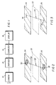
- the present invention as illustrated in Figure 1, is implemented using conventional image processing equipment.
- the equipment includes one or more cameras 10 that captures stereo images on film.
- the film images are digitized by a conventional digitizer 12.
- An electronic camera can of course substitute for the film camera and digitizer.
- the digitizer images are supplied to a computer 14 which performs the process discussed herein to create intermediate images.
- the images are interlaced and provided to a display device 16.
- the display device 16 can be a CRT with a lenticular or barrier strip faceplate or it can be a print or transparency printer which produces a print to which a lenticular or barrier strip faceplate is attached.
- optical flow This vector field is commonly referred to as the optical flow (see Robot Vision, B.K.P. Horn, The MIT Press, 1991).
- One of the well-known characterizations of optical flow is that depth is inversely proportional to the magnitude of the optical flow vector. In this instance the zero parallax plane occurs in object space where the optical flow vectors have magnitude zero, i.e., points unaffected by the change of camera position, such as the background.
- the first step is to find correspondences between the pair of images 24 and 26.
- a vector or line 28 passing through the pixel 20 being created in the intermediate image is used to designate different areas on the images 24 and 26 are to be compared.
- the point of incidence on the images 24 and 26 can be systematically moved about two dimensional areas 30 and 32 searching for the areas that have the highest correlation in spectral and other image characteristics. Once these points are found the correspondences can be used to interpolate the value of the intermediate pixel 20.
- the correspondences between two images in two dimensions does not have a unique solution and, as a result, a search process as illustrated in Figure 2 may not produce the best solution.
- the solution is not unique it is necessary to perform smoothing of the image to reduce or eliminate noise artifacts created in the intermediate image 22.
- the cameras used in obtaining the stereo image pair are assumed to be positioned parallel to the plane of the scene spanning the horizontal and vertical axes, and the changes in the camera positions are assumed to be strictly in the horizontal direction. It is assumed that the horizontal and the vertical axes of each image of the stereo image pair coincide with the horizontal and the vertical axes of the scene. Under these assumptions the correspondence between the images of the stereo image pair can be characterized by the intermediate disparity vector field with the constant vertical component relating to the alignment of the images and with the variable horizontal component relating to the depths of the corresponding points in the scene.
- each band of the right and the left digital images is defined as a two-dimensional array of numbers representing some measurements, known as pixels, taken from some grid of points ⁇ '' on the sensed image. In the preferred embodiment, this grid is assumed to be a rectangular lattice.
- the estimate of the intermediate image band I b,k is obtained 60 by the interpolation process.
- the depth image band D b is constructed by interlacing the intermediate image bands I b,1 ,...,I b,K to produce the depth image 62.
- the method of estimating the intermediate disparity vector field (U k ,V k ) at the intermediate viewpoint t k is illustrated in Figure 5 and can be described as the following multi-level resolution process: 1) Start 70 with the coarsest resolution level and the current estimate of the intermediate disparity vector field, (initially set to some constant); 2) Iteratively 72-82 improve the current estimate; 3) Project 84 to the next finer level of resolution to obtain the initial estimate of the intermediate disparity vector field at the next finer level which is taken as the current estimate of the intermediate disparity vector field; 4) Repeat steps 2) and 3) until the finest resolution level is reached.
- the proper estimate of the finest resolution level is taken as the final estimate of the intermediate disparity vector field.
- a system of nonlinear equations relative to the unknown current estimate of the intermediate disparity vector field is formed 76, then iterative improvement of the current estimate of the intermediate disparity vector field is achieved by solving 78 this system of nonlinear equations.
- the system of nonlinear equations relative to the unknown current estimate of the intermediate disparity vector field is defined in terms of the unknown current estimate of the intermediate disparity vector field, the quantities related to the right and to the left pixels and the generalized spatial partial derivatives of the right and the left images. These quantities are obtained by filtering each band of the right and the left images with filters ⁇ 1,... ⁇ F and with the spatial partial derivatives of these filters.
- the symbol G is used for the set of indices with each index g ⁇ G specifying a particular band and a particular filter.
- the multi-level resolution process (See U.S. application 631,750 incorporated by reference herein) is built around a multi-level resolution pyramid meaning that on each coarser resolution level the filtered right and the filtered left images, their spatial partial derivatives and the estimates of the intermediate disparity vector fields are defined on subgrids of grids at a finer resolution level.
- the bands of the filtered right images, the spatial partial derivatives of the bands of the filtered right images, the bands of the filtered left images, and the spatial partial derivatives of the bands of the filtered left images are defined on the same grid of points ⁇ ' on the image plane of size N by M .
- the intermediate disparity vector fields are defined on a grid of points ⁇ on the image plane of size N by M.
- each image point of the grid ⁇ is shifted by the amount equal to the scaled by the factor (t R -t k )/(t R -t L ) value of the estimated intermediate disparity vector defined at that grid point.
- each image point of the grid ⁇ is shifted by the amount equal to the scaled by the factor (t k -t L )/(t R -t L ) value of the estimated intermediate disparity vector defined at that grid point.
- index g ⁇ G specifying a particular filter and a particular image band, form a spatial partial derivative g tu of the optical flow function g t with respect to the component u of the current estimate of the intermediate disparity vector corresponding to the index g as the defined on the grid ⁇ sum of the scaled by the factor (t R -t k )/(t R -t L ) spatial partial derivative of the estimated right filtered image band and the scaled by the factor (t k -t L )/(t R -t L ) spatial partial derivative of the estimated left filtered image band.
- the spatial partial derivative of the estimated right filtered image band To obtain the spatial partial derivative of the estimated right filtered image band, find the grid of image points ⁇ R which are taken from the viewpoint t R estimated perspective projections onto the image plane of the visible points in the scene, whose perspective projections onto the image plane from the viewpoint t k are the grid points ⁇ ; and then interpolate the spatial partial derivatives of the right filtered image from the grid of points ⁇ ' where the spatial partial derivative of the right filtered image is defined to the grid of points ⁇ R .
- each image point of the grid ⁇ is shifted by the amount equal to the scaled by the factor (t R -t k )/(t R -t L ) value of the estimated intermediate disparity vector defined at that grid point.
- each image point of the grid ⁇ is shifted by the amount equal to the scaled by the factor (t k -t L )/(t R -t L ) value of the estimated intermediate disparity vector defined at that grid point.
- index g ⁇ G specifying a particular filter and a particular image band, form a spatial partial derivative g tv of the optical flow function g t with respect to the component v of the current estimate of the intermediate disparity vector corresponding to the index g as the defined on the grid ⁇ sum of the scaled by the factor (t R -t k )/(t R -t L ) spatial partial derivative with respect to the vertical component of the image coordinate system of the estimated right filtered image band corresponding to the index g and the scaled by the factor (t k -t L )/(t R -t L ) spatial partial derivative with respect to the vertical component of the image coordinate system of the estimated left filtered image band corresponding to the index g.
- the spatial partial derivative with respect to the vertical component of the image coordinate system of the estimated right filtered image band find the grid of image points ⁇ R which are the taken from the viewpoint t R estimated perspective projections onto the image plane of the visible points in the scene, whose perspective projections onto the image plane from the viewpoint t k are the grid points ⁇ ; and then interpolate the spatial partial derivatives with respect to the vertical component of the image coordinate system of the right filtered image from the grid of points ⁇ ' where the spatial partial derivative with respect to the vertical component of the image coordinate system of the right filtered image is defined to the grid of points ⁇ R .
- the spatial partial derivative with respect to the vertical component of the image coordinate system of the estimated left filtered image band find the grid of image points ⁇ L which are taken from the viewpoint t L estimated perspective projections onto the image plane of the visible points in the scene, whose perspective projections onto the image plane from the viewpoint t k are the grid points ⁇ ; and then interpolate the spatial partial derivatives with respect to the vertical component of the image coordinate system of the left filtered image from the grid of points ⁇ ' where the spatial partial derivative with respect to the vertical component of the image coordinate system of the left filtered image is defined to the grid of points ⁇ L .
- each image point of the grid ⁇ is shifted by the amount equal to the scaled by the factor (t R -t k )/(t R -t L ) value of the estimated intermediate disparity vector defined at that grid point.
- each image point of the grid ⁇ is shifted by the amount equal to the scaled by the factor (t k -t L )/(t R -t L ) value of the estimated intermediate disparity vector defined at that grid point.
- Each non-boundary grid point of the rectangular grid ⁇ is surrounded by its eight nearest neighbors specifying eight different directions on the image plane. For each boundary grid point of the rectangular grid ⁇ the nearest neighbors are present only for some of these eight different directions.
- the symbol s is used to denote a vector on the image plane specifying one of these eight different directions on the image plane.
- the symbol S is used to denote the set of these eight vectors. For each vector s from the set S specifying a particular direction on the image plane, form a directional smoothness function (s, ⁇ u) for the variable horizontal component in of the current estimate of the intermediate disparity vector field as a finite difference approximation to the directional derivative of the horizontal component u of the current estimate of the intermediate disparity vector field.
- This directional smoothness function (s, ⁇ u) is defined on the rectangilar subgrid ⁇ s of the rectangular grid ⁇ with the property that every grid point of the rectangilar subgrid ⁇ s has the nearest in the direction s neighbor on the rectangular grid ⁇ .
- the directional smoothness function (s, ⁇ u) is equal to the difference between the value of the horizontal component u of the current estimate of the intermediate disparity vector field at the nearest in the direction s neighbor of this grid point and the value of the horizontal component u of the current estimate of the intermediate disparity vector field at this grid point.
- the system of nonlinear equations relative to the unknown current estimate of the intermediate disparity vector field is formed by combining the optical flow function g t and its spatial partial derivatives g tu , g tv for each filter and each image band specified by the index g ⁇ G together with the directional smoothness function (s, ⁇ u) for each image direction s ⁇ S and together with some constant parameters using four basic algebraic operations such as addition, subtraction, multiplication and division.
- the method of estimating the intermediate digital image taken at the intermediate viewpoint t k and consisting of the bands I 1,k ,...,I B,k based on the estimate of the intermediate disparity vector field (U k ,V k ) obtained at the intermediate viewpoint t k can be described as follows.
- the estimate of the intermediate digital image band I b,k is defined as the sum of the scaled by the factor (t k -t L )/(t R -t L ) estimated right digital image band and the scaled by the factor (t R -t k )/(t R -t L ) estimated left digital image band.
- the estimated right digital image band To obtain the estimated right digital image band, find the grid of image points ⁇ R which are the taken from the viewpoint t R estimated perspective projections onto the image plane of the visible points in the scene, whose perspective projections onto the image plane from the viewpoint t k are the grid points ⁇ ; and then interpolate the right digital image band from the grid of points ⁇ '' where the right digital image is defined to the grid of points ⁇ R .
- each image point of the grid ⁇ is shifted by the amount equal to the scaled by the factor (t R -t k )/(t R -t L ) value of the estimated intermediate disparity vector defined at that grid point.
- each image point of the grid ⁇ is shifted by the amount equal to the scaled by the factor (t k -t L )/(t R -t L ) value of the estimated intermediate disparity vector defined at that grid point.
- the initial images of a three-dimensional scene are, in general, discontinuous functions and their spatial partial derivatives are not defined at the points of discontinuity.
- the points of discontinuity are, often, among the most important points in the images and cannot be easily ignored.
- the initial images are treated as generalized functions and their partial derivatives as generalized partial derivatives.
- These generalized functions are defined on some subset of the set of infinitely differentiable functions. The functions from the subset are called "testing functions”.
- Parametric families of secondary images are then introduced through evaluations of the generalized functions associated with the initial images on the specific parametric family of functions taken from the set of testing functions.
- the secondary images are infinitely differentiable, and their partial derivatives can be obtained through evaluations of the generalized functions associated with the initial images on the partial derivatives of this specific parametric family of functions. This process can be described as follows.
- R is a one-dimensional Euclidean space
- image plane two-dimensional Euclidean space
- the value ⁇ (x,y,t) of the irradiance image function at the point (x,y) ⁇ R2 and the viewpoint t ⁇ R is assumed to be roughly proportional to the radiance of the point in the scene being imaged, which projects to such a point (x,y) at the viewpoint t for every (x,y) ⁇ R2 and every t ⁇ R.
- Different irradiance image functions ⁇ (x,y,t), (x,y,t) ⁇ R3 can be obtained by changing the following aspects of the image formation process: the direction of a light source illuminating the scene, the color of such a light source, and the spectral responsivity function that is used to compute the irradiance.
- each irradiance image function ⁇ (x,y,t) is locally integrable with respect to the Lebesgue measure dx dy dt in R3 and thereby can be used to form a continuous linear functional ⁇ ⁇ (generalized function) defined on the locally convex linear topological space ⁇ (R3).
- the space ⁇ (R3) consists of all infinitely differentiable functions having compact supports in the set R3. This means that for each function ⁇ (R3) there exists a closed bounded subset S ⁇ ⁇ R3 such that the function ⁇ is equal to zero at the points that are outside the subset S ⁇ .
- the topology of the space ⁇ (R3) is defined by a certain family of semi-norms.
- the functions ⁇ from the set ⁇ (R3) will be called the "testing functions".
- the value of the generalized function ⁇ ⁇ associated with the irradiance image function ⁇ at the testing function ⁇ (R3) is defined by the following relation:
- the generalized functions ⁇ ⁇ associated with different irradiance image functions ⁇ (x,y,t) are united into the family ⁇ ⁇
- the symbol ⁇ takes the role of the index (parameter) specifying the generalized function ⁇ ⁇ associated with a particular irradiance image function ⁇ (x,y,t) in addition to its role as a part of the notation for such an irradiance image function.
- the symbol ⁇ denotes the set of indices.
- Another way of constructing an initial image at a given viewpoint t ⁇ R is by identifying the set of points M(t) ⁇ R2 in the image plane, called the “feature points", where significant variations in the projected light patterns represented by the irradiance image functions take place at the viewpoint t, and then assigning feature value ⁇ (x ⁇ ,y ⁇ ,t ⁇ ) to each feature point (x ⁇ ,y ⁇ ,t ⁇ ) ⁇ M(t).
- the set of feature points is assumed to be a closed subset of the space R3.
- the function ⁇ (x ⁇ ,y ⁇ ,t ⁇ ) defined on the set M as above will be called the "feature image function".
- Different feature image functions ⁇ (x ⁇ ,y ⁇ ,t ⁇ ), (x ⁇ ,y ⁇ ,t ⁇ ) ⁇ M can be obtained by changing the criteria for selecting the set of feature points M and the criteria for assigning the feature values ⁇ (x ⁇ ,y ⁇ ,t ⁇ ).
- the set M may, for example, be a finite combination of the following four types of the subsets of the space R3: the three-dimensional regions, the two-dimensional regions, the one-dimensional contours, and the isolated points.
- ⁇ B(M) of "Borel subsets" of the set M shall be meant the members of the smallest ⁇ -finite, ⁇ -additive family of subsets of M which contains every compact set of M.
- ⁇ (B) be a ⁇ -finite, ⁇ -additive, and real-valued measure defined on the family B of Borel subsets of the set M.
- the feature image function ⁇ (x ⁇ ,y ⁇ ,t ⁇ ),(x ⁇ ,y ⁇ ,t ⁇ ) ⁇ M is assumed to be ⁇ -measurable and thereby can be used to form a continuous linear functional ⁇ ⁇ (generalized function) defined on the locally convex linear topological space ⁇ (R3).
- the value of the generalized function ⁇ ⁇ associated with the feature image function ⁇ at the testing function ⁇ (R3) is given by the following relation:
- the generalized functions ⁇ ⁇ associated with different feature image functions ⁇ (x ⁇ ,y ⁇ ,t ⁇ ) are united into the family ⁇ ⁇
- the symbol ⁇ takes the role of the index (parameter) specifying the generalized function ⁇ ⁇ associated with a particular feature image function ⁇ (x ⁇ ,y ⁇ ,t ⁇ ) in addition to its role as a part of the notation for such a feature image function.
- the symbol H denotes the set of indices.
- the "generalized partial derivative" of the generalized function F is the generalized function defined on the locally convex linear topological space ⁇ (R3) as follows.
- the value of the generalized function at a testing function ⁇ (R3) is the value of the generalized function F itself at the testing function
- a "combined generalized initial image function” will be defined as a linear combination of the generalized partial derivatives of the generalized functions associated with the irradiance image functions and of the generalized partial derivatives of the generalized functions associated with the feature image functions.
- ⁇ , ⁇ H ⁇ be a set of real-valued constants
- g( ⁇ ) be an index attached to the set ⁇
- ⁇ , ⁇ H ⁇ be a set of non-negative integer constants corresponding to the set of constants ⁇ .
- the combined generalized initial image function corresponding to the set of constants ⁇ is the generalized function ⁇ g( ⁇ ) defined on the locally convex linear topological space ⁇ (R3).
- the value of the combined generalized initial image function ⁇ g( ⁇ ) corresponding to the set of constants ⁇ at the testing function ⁇ (R3) is given by the relation and is called the "observation" of the combined generalized initial image function ⁇ g( ⁇ ) corresponding to the set of constants ⁇ on the testing function ⁇ .
- the combined generalized initial image functions ⁇ g( ⁇ ) corresponding to sets of constants ⁇ with different values are united into the family ⁇ g( ⁇ )
- the symbol ⁇ denotes the family of all different sets of constants ⁇
- the symbol g denotes the one-to-one mapping from the family ⁇ onto the set of indices denoted by the symbol G.
- the argument ⁇ appearing in the notation for a combined generalized initial image function is omitted and the symbol ⁇ g , g ⁇ G is used instead of the symbol ⁇ g( ⁇ ) , ⁇ to denote it.
- the points (x,y,t) from the set ⁇ ⁇ T will be called “viewpoint-varying image points”.
- image corresponding to the parameter value ⁇ [1, ⁇ ) and taken at the viewpoint t ⁇ T is meant the collection, ⁇ g ⁇ (x,y,t)
- (x,y) ⁇ corresponding to every parameter value ⁇ [1, ⁇ ) and taken at a fixed viewpoint t ⁇ T will be called the "parametric image" taken at the viewpoint t.
- Each component g ⁇ (x,y,t), g ⁇ G of the parametric viewpoint-varying image function g ⁇ (x,y,t) is infinitely differentiable everywhere in the domain ⁇ ⁇ T, and its partial derivatives with respect to the variables x, y, t can be obtained as observations of the combined generalized initial image function ⁇ g on the partial derivatives with respect to the parameters x, y, t of the testing function ⁇ ⁇ x,y,t ⁇ (R3) specified by the relation (2-4).
- g ⁇ G ⁇ of the parametric viewpoint-varying image function g ⁇ (x,y,t) are given as the observations of the combined generalized initial image function ⁇ g on the testing functions for every (x,y,t) ⁇ T, ⁇ [1, ⁇ ), where and ⁇ x (x,y,t), ⁇ y (x,y,t) are the partial derivatives of the function ⁇ (x,y,t) with respect to the variables x,y.
- the vector (u A (x,y,t, ⁇ t ⁇ , ⁇ t+), v A (x,y,t, ⁇ t ⁇ , ⁇ t+)) can be defined only at those points (x,y) from the set R2 that are projections of the points in the scene visible at the viewpoint t- ⁇ t ⁇ as well as the viewpoint t+ ⁇ t+.
- the collection of such image points will be denoted by the symbol ⁇ (t, ⁇ t ⁇ , ⁇ t+).
- the set W(x,y,t, ⁇ t) will be defined from the relation while the set W(x,y,t) will be defined as where the symbol W ( x,y,t, ⁇ t ) ⁇ means the topological closure of the set W(x,y,t, ⁇ t). It will be assumed that W(x,y,t) are single-element sets for almost every (x,y,t) ⁇ R3. This assumption means that the subset of the set R3 containing the points (x,y,t), where the sets W(x,y,t) are not single-element sets, has a Lebesgue measure equal to zero.
- (x,y) ⁇ corresponding to the viewpoint t ⁇ T and to the parameter value ⁇ [1, ⁇ ) will be called the "velocity vector field" of the image ⁇ g ⁇ (x,y,t)
- (x,y) ⁇ corresponding to every parameter value ⁇ [1, ⁇ ) and taken at a fixed viewpoint t ⁇ T will be called the "parametric velocity vector field" of the parametric image ⁇ g ⁇ (x,y,t)
- the method of the present invention includes determining an estimate of the parametric velocity vector field corresponding to a given parametric viewpoint-varying image sequence.
- determining an estimate of the parametric velocity vector field corresponding to a given parametric viewpoint-varying image sequence In order for this determination to be possible, specific assumptions have to be made about the scene being imaged and about the imaging process itself. The assumptions we make are described in the following. Based on these assumptions constraints are imposed on the estimate of the parametric velocity vector field. The determination of the estimate is then reduced to solving the system of equations arising from such constraints for a given parametric viewpoint-varying image sequence.
- (x,y) ⁇ , ⁇ [1, ⁇ ) ⁇ is determined as the parametric vector field satisfying a set of constraints. These constraints are based on the following assumptions:
- ⁇ t be a subset of the space R2 defined by the relation let P t be a subset of the set ⁇ t , and let G t ⁇ G ⁇ P t be the Cartesian product of the set G on the set P t .
- the elements from the set G t are denoted by the symbol g t , and the set G t is assumed to be a measurable space with some measure dg t defined on the family B(G t ) of Borel subsets of the set G t .
- the set G t is finite
- the measure dg t is a point measure on the finite set G t , but a more general approach is used for the sake of uniformity of presentation.
- the symbol g t is used as the part of the notation g t ⁇ for the above defined function (3-2) in addition to its role as the index for such a function.
- (x,y) ⁇ be an image point that is taken at the viewpoint t projection of some point in the scene that does not belong to the occluding boundaries.
- the occluding boundary of an object is defined as the points in the scene belonging to the portion of the object that projects to its silhouette.
- the assumptions 1-4 made at the beginning of this section imply that the absolute value of the function g t ⁇ (x,y,t,u ⁇ ,v ⁇ ) is small. Therefore it is natural to use the function as a part of the functional whose minimum specifies the estimate of the velocity vector (u ⁇ (x,y,t),v ⁇ (t)) of the image corresponding to the parameter value ⁇ .
- thin function (3-3) to be called the "optical flow constraint" corresponding to the parameter value ⁇ and the index g t [2, 12-14, 18-21].
- the viewpoint increments ⁇ t ⁇ , ⁇ t+ approach zero then for an integer n greater than or equal to 2 the n th-order partial derivative of the function g t ⁇ (x,y,t, ⁇ , ⁇ ) with respect to the components of the estimate of the velocity vector approaches zero at a rate proportional to ( ⁇ t ⁇ ) n-1 +( ⁇ t+) n-1 .
- This implies that when the viewpoint increments ⁇ t ⁇ , ⁇ t+ approach zero the function g t ⁇ (x,y,t, ⁇ , ⁇ ) approaches the function which is linear with respect to the components ⁇ , ⁇ of the estimate of the velocity vector.
- the estimate ( ⁇ (x,y,t), ⁇ (t)) of the velocity vector on which the function (3-3) achieves its minimum satisfies the system of equations where the functions g t ⁇ (x,y,t, ⁇ , ⁇ ) and g t ⁇ (x,y,t, ⁇ , ⁇ ) are the first-order partial derivatives of the function g t ⁇ (x,y,t, ⁇ , ⁇ ) with respect to the components ⁇ and ⁇ of the estimate of the velocity vector.
- the initial estimate ( 0 ⁇ (x,y,t), 0 ⁇ (t)) appearing in the relations (3-12), (3-13) is defined later in this section.
- the optical flow and the directional smoothness constraints are not necessarily valid at the points near the occluding boundaries, even when the assumptions described at the beginning of this section are observed.
- the method of computing the estimate of the parametric velocity vector field of the present invention resolves the above difficulties by adjusting the weight associated with each constraint in such a way that it becomes small whenever the constraint is not valid.
- the functions (3-3), (3-11), (3-12), and (3-13), specifying the optical flow, directional smoothness, and regularization constraints are combined into the functional of the estimate of the parametric velocity vector field.
- the estimate is then computed by solving the system of nonlinear equations arising from a certain optimality criterion related to such functional.
- (x,y) ⁇ , ⁇ [1, ⁇ ) ⁇ is determined as the parametric vector field on which a weighted average of the optical flow, directional smoothness, and regularization constraints is minimized.
- each weight function associated with an optical flow constraint becomes small whenever the optical flow constraint is not satisfied
- each weight function associated with a smoothness constraint corresponding to a direction in which an occluding boundary is crossed becomes small whenever the directional smoothness constraint is not satisfied.
- each weight function has to be treated as if it were independent of the values of the unknown estimate of the parametric velocity vector field, because it only specifies a relative significance of the corresponding constraint as a part of the weighted average and not the constraint itself.
- two copies of the unknown estimate of the parametric velocity vector field are introduced: the invariable one, and the variable one.
- the invariable copy of the unknown estimate of the parametric velocity vector field are used, whereas in the constraint functions the values of the variable copy of the unknown estimate of the parametric velocity vector field are used.
- f ( , , , ) be a functional of the parametric vector fields ( , ),( , ) defined as a weighted average of functions (3-3), (3-11), (3-12), and (3-13), specifying the optical flow, directional smoothness, and regularization constraints, respectively, by the following relation:
- f ( , , , ) be a functional of the parametric vector fields ( , ),( , ) defined as a weighted average of functions (3-3), (3-11), (3-12), and (3-13), specifying the optical flow, directional smoothness, and regularization constraints, respectively, by the following relation:
- the estimate of the parametric velocity vector field is then defined as the parametric vector field ( , ), on which the functional f ( , , , ), considered as the function of the parametric vector field ( , ) and depending on the parametric vector field ( , ) as on the parameters, achieves a local minimum when the value of the parametric vector field ( , ) is identically equal to the value of the parametric vector field ( , ).
- the functional f ( , , ) can be expressed in the form f ( , , + ⁇ , + ⁇ ).
- the parametric vector field ( ⁇ , ⁇ ) specifies a perturbation to the parametric vector field ( , ), and the functional f ( , , + ⁇ , + ⁇ ) assigns the cost to each choice of the parametric vector field ( , ) and its perturbation ( ⁇ , ⁇ ). Then the estimate of the parametric velocity vector field is the parametric vector field ( , ), for which a locally minimal cost is achieved when the perturbation ( ⁇ , ⁇ ) is identically equal to zero.
- the above defined estimate ( , ) of the parametric velocity vector field is a solution of the system of equations where the functions g t ⁇ (x,y,t, ⁇ , ⁇ ) and g t ⁇ (x,y,t, ⁇ , ⁇ ) are the first-order partial derivatives of the function g t ⁇ (x,y,t, ⁇ , ⁇ ) with respect to the components and of the estimate of the velocity vector.
- each of the weight functions ⁇ s ⁇ (x,y,t, ⁇ , ⁇ ,(s, ⁇ ⁇ )), s ⁇ S will be chosen so that the contributions of the directional smoothness constraint (s, ⁇ ⁇ (x,y,t)) to the functional (4-5) become small for every image point (x,y) ⁇ located near the occluding boundary where the occluding boundary is crossed in the direction s and the directional smoothness constraint (s, ⁇ ⁇ (x,y,t)) is not satisfied.
- the image point (x,y) ⁇ be near the occluding boundary; then the following two events are likely to happen:
- the image point (x,y) does not necessarily lie near the occluding boundary. It may, for example, lie on the object of the scene whose projection onto the image plane undergoes a rotation or a local deformation. Also note that in the case of some of the functions (S, ⁇ 'g t ⁇ (x,y,t, ⁇ , ⁇ )), g t ⁇ G t being large, the image point (x,y) does not necessarily cross the occluding boundary in the direction s. It may, for example, cross the radiance boundary arising from a texture or a sudden change in the illumination.
- each of the weight functions should be a steadily decreasing function relative to the absolute value of the function g t ⁇ (x,y,t, ⁇ , ⁇ ) and to the values of the function
- the values of the estimates of the velocity vector field corresponding to the different values of the parameter a are tied together by imposing the following restriction: the estimate of the parametric velocity vector field ⁇ ( ⁇ (x,y,t), ⁇ (t))
- (x,y) ⁇ , ⁇ [1, ⁇ ) ⁇ are imposed in the form of the boundary conditions as follows:
- ⁇ [1, ⁇ ) be a given parameter value, and let ⁇ be an infinitesimal positive real value.
- Such an action reflects the fact that in this case the image point (x,y) is likely to cross the occluding boundary in the direction s if the value of the function (s, ⁇ ⁇ (x,y,t))2 specifying the degree of the smoothness of the estimate of the velocity vector field in such a direction s is large.
- the role of the regularization constraint is to discriminate between the parametric vector fields ( , ) giving the same optimal values to the weighted average of the optical flow and the directional smoothness constraints without causing any significant changes in these values. This is achieved by assigning small values to the parameters ⁇ u and ⁇ v appearing in the system of nonlinear equations (4-19). For the sake of simplicity of the analysis given below, we shall ignore the regularization constraints by assuming that the parameters ⁇ u and ⁇ v are equal to zero while keeping in mind that the solution of the system of nonlinear equations (4-19) is locally unique.
- the parameters r2 and a2 have their greatest impact on the solution of the system of nonlinear equations (4-19) at the image points that are away from the occluding boundary, while the parameters mostly influence the solution at the image points that are near the occluding boundary.
- the parameter r2 defines the coefficient of proportionality for the functions g t ⁇ (x,y,t, ⁇ , ⁇ ),g t ⁇ G t specifying the optical flow constraints, while the parameter a2 determines the proportionality coefficient for the function (s, ⁇ ⁇ (x,y,t)),s ⁇ S specifying the directional smoothness constraints.
- the combination (4-24) of the parameters r2, p2, and q2 determines the upper limit for the influence of the optical flow constraints on the solution of the system of nonlinear equations (4-19), while the combination (4-27) of the parameters a2, c2 and determines the upper limit for the influence of the directional smoothness constraints on the solution of the system of nonlinear equations (4-19).
- the symbols t ⁇ , t ⁇ , t ⁇ , t ⁇ have been used instead of the symbols g t ⁇ , g t ⁇ ,g t ⁇ ,g t ⁇ to indicate that at every image point (x,y) ⁇ the corresponding functions depend on the estimate ( ⁇ (x,y,t), ⁇ (t)) of the velocity vector (u ⁇ (x,y,t),v ⁇ (t)).
- the system of nonlinear equations (5-7) relative to the unknown estimate of the velocity vector field corresponding to the parameter value ⁇ defines, for every image point (x,y) ⁇ , a set of relations between the components of the velocity vector ( ⁇ (x,y,t), ⁇ (t)) and its partial derivatives, which can be expressed in the form
- the estimate ( ⁇ , ⁇ ) of the velocity vector field corresponding to the parameter value ⁇ as an estimate of the solution of the system of nonlinear equations (5-7) corresponding to the parameter value ⁇ that is the closest to the initial estimate ( ⁇ ( ⁇ ) , ⁇ ( ⁇ ) ) the iterative updating scheme can be used.
- the improved estimate of the solution of the system of nonlinear equations (5-7) corresponding to the parameter value ⁇ is determined by the step where the scalar parameter defines the length of the step, while the vector field defines the direction of the step.
- the step length ⁇ (0,1] is selected in such a way that the following function is minimized:
- the step direction ( ⁇ ⁇ , ⁇ ⁇ ) is selected in such a way that the function (5-10) becomes steadily decreasing for sufficiently small values of ⁇ (0,1].
- the improved estimate ( + ⁇ , + ⁇ ) is taken as the current estimate ( ⁇ , ⁇ ) of the solution of the system of nonlinear equations (5-7) corresponding to the parameter value ⁇ , and the step (5-9) of the iterative updating scheme is repeated to determine the next improved estimate ( + ⁇ , + ⁇ ) of the solution of the system of nonlinear equations (5-7) corresponding to the parameter value ⁇ . This process is continued until the appropriate criteria are met, in which case the improved estimate ( + ⁇ , + ⁇ ) is taken as the estimate ( ⁇ , ⁇ ) of the velocity vector field corresponding to the parameter value ⁇ .
- the nonlinear operator F ⁇ can be linearly expanded as
- the linear and bounded with respect to the vector field ( ⁇ ⁇ , ⁇ ⁇ ) operator J ⁇ ( ⁇ , ⁇ , ⁇ ⁇ , ⁇ ⁇ ) is the Jacobian of the nonlinear operator F ⁇ ( ⁇ , ⁇ ) .
- the operator J ⁇ ( ⁇ , ⁇ , ⁇ ⁇ , ⁇ ⁇ ) can be more conveniently expressed in the form
- the vector field ( ⁇ ⁇ , ⁇ ⁇ ) is defined as a solution of the system of linear equations
- the improved estimate ( + ⁇ , + ⁇ ) of the solution of the system of nonlinear equations (5-7) is defined as in the relation (5-9) where the scalar parameter is taken to be equal to 1.
- the improved estimate ( + ⁇ , + ⁇ ) of the solution of the system of nonlinear equations (5-7), which is obtained as the result of solving the system of linear equations (5-13) and then applying the relation (5-9), is not necessarily a better estimate.
- the reason behind it comes from the fact that the Jacobian J ⁇ ( ⁇ , ⁇ ) of the nonlinear operator F ⁇ ( ⁇ , ⁇ ) is nonsymmetric and ill-conditioned, so that the system of linear equations (5-13) cannot be reliably solved for the vector field ( ⁇ ⁇ , ⁇ ⁇ ).
- F ⁇ ⁇ ( ⁇ , ⁇ , ⁇ , ⁇ ), ⁇ [0,1] be a family of nonlinear operators of the invariable copy ( ⁇ , ⁇ ) and of the variable copy ( ⁇ , ⁇ ) of the estimate of the velocity vector field corresponding to the parameter value ⁇ defined by the relation where the symbols t ⁇ , t ⁇ , t ⁇ , t ⁇ , t ⁇ are used to indicate that at every image point (x,y) ⁇ the corresponding functions depend on the invariable copy ( ⁇ (x,y,t), ⁇ (t)) of the estimate of the velocity vector (u ⁇ (x,y,t),v ⁇ (t)), while the symbol ⁇ t ⁇ is used to indicate that at every image point (x,y) ⁇ the corresponding function depends on the variable copy (û ⁇ (x,y,t),v ⁇ ⁇ (t)) of the estimate of the velocity vector (u ⁇ (x,y,t),
- variable copy ( ⁇ , ⁇ ) of the estimate of the velocity vector field is identically equal to the invariable copy ( ⁇ , ⁇ ) of the estimate of the velocity vector field, then for every ⁇ [0,1] the nonlinear operator F ⁇ ⁇ ( ⁇ , ⁇ , ⁇ , ⁇ ) is identically equal to the nonlinear operator F ⁇ ( ⁇ , ⁇ ) .
- the parameter ⁇ defines the degree of the feedback relaxation of the optical flow and the directional smoothness constraints through the variable copy ( ⁇ , ⁇ ) of the estimate of the velocity vector field.
- M ⁇ ⁇ ( ⁇ , ⁇ )( ⁇ ⁇ , ⁇ ⁇ ) , ⁇ [0,1] be a family of the linear and bounded with respect to the vector field ( ⁇ ⁇ , ⁇ ⁇ ) operators, where for each ⁇ [0,1] the operator M ⁇ ⁇ ( ⁇ , ⁇ )( ⁇ ⁇ , ⁇ ⁇ ) is the Jacobian of the nonlinear operator F ⁇ ⁇ ( ⁇ , ⁇ , ⁇ , ⁇ ) , considered as the function of the vector field ( ⁇ , ⁇ ) , and depending on the vector field ( ⁇ , ⁇ ) as on the parameter, under the conditions that the vector field ( ⁇ , ⁇ ) is identically equal to the vector field ( ⁇ , ⁇ ) .
- F be a generalized function
- ⁇ (R3) be a given fixed non-negative testing function such that For instance, take where ⁇ is the function described later.
- the testing function ⁇ will be called the "sampling function”.
- the "regularisation" of the generalized function F through the sampling function ⁇ is defined on the space R3 as the infinitely differentiable function (F* ⁇ ), which is obtained as the convolution of the generalized function F and the sampling function ⁇ .
- the regularizations ⁇ ⁇ ⁇ ( ⁇ ⁇ * ⁇ ) of the generalized functions ⁇ ⁇ associated with the irradiance image functions ⁇ , ⁇ through the sampling function ⁇ and the regularizations ⁇ ( ⁇ * ⁇ ) of the generalized functions ⁇ associated with the feature image functions ⁇ , ⁇ H through the sampling function ⁇ are given at the points (x,y) belonging to the following subset of the image plane:
- Z is the set of integers
- h' ⁇ ,1 ,h' ⁇ ,2 are two-dimensional real vectors
- i1h' ⁇ ,1 +i2h' ⁇ ,2 is a linear combination of such vectors with integer coefficients i1,i2.
- the points from the set R2(h' ⁇ ,1 ,h' ⁇ ,2 ) will be called the “sampling points" corresponding to the parameter ⁇ ; the functions ⁇ , ⁇ will be called the “sampled irradiance image functions"; and the functions ⁇ , ⁇ H will be called the “sampled feature image functions”.
- the generalized functions ⁇ ⁇ , ⁇ associated with the sampled irradiance image functions ⁇ ⁇ , ⁇ and the generalized functions ⁇ ⁇ , ⁇ associated with the sampled feature image functions ⁇ ⁇ , ⁇ H are defined on the set of testing functions ⁇ (R3) as follows.
- the value of the generalized function ⁇ ⁇ , ⁇ associated with the sampled irradiance image function ⁇ ⁇ at the testing function ⁇ (R3) is given by the relation
- the value of the generalized function ⁇ ⁇ , ⁇ associated with the sampled feature image function ⁇ ⁇ at the testing function ⁇ (R3) is given by the relation
- ⁇ , ⁇ H ⁇ be a set of real-valued constants
- g( ⁇ ) be an index attached to the set ⁇
- ⁇ , ⁇ H ⁇ be a set of non-negative integer constants corresponding to the set of constants ⁇ .
- the "combined generalized sampled image function" corresponding to the index g ⁇ g( ⁇ ) is the generalized function ⁇ g, ⁇ defined on the locally convex linear topological space ⁇ (R3).
- the value of the combined generalized sampled image function ⁇ g, ⁇ at the testing function ⁇ (R3) is given by the relation and is called the "observation" of the combined generalized sampled image function ⁇ g, ⁇ on the testing function ⁇ .
- the image point (x,y) belongs to the subset ⁇ ''(h'' ⁇ ,1 ,h'' ⁇ ,2 ) ⁇ R2(h'' ⁇ ,1 ,h'' ⁇ ,2 ).
- the two-dimensional real vectors h'' ⁇ ,1 ,h'' ⁇ ,2 are defined as in the relations while the set ⁇ ''(h'' ⁇ ,1 ,h'' ⁇ ,2 ) ⁇ R2 is defined as in the relation
- the value of the component g ⁇ (x,y,t) of the image function g ⁇ (x,y,t) is determined as the observation ⁇ g, ⁇ ( ⁇ x,y,t ⁇ ) of the combined generalized sampled image function ⁇ g, ⁇ on the testing function ⁇ x,y,t ⁇ defined by the relation (2-4); and the values of the components g x ⁇ (x,y,t),g y ⁇ (x,y,
- the unit circle making up the set S is replaced by a finite set, denoted by the same symbol S, of the set R2(h ⁇ ,1 ,h ⁇ ,2 ) having the following properties: the set S does not contain the origin, and for every element s belonging to the set S the element -s also belongs to the set S.
- the measure ds is replaced with the point measure associating the value 0.5 to every element s ⁇ S.
- the functions t ⁇ , t ⁇ , t ⁇ are defined, respectively, by the relations
- 2 is defined as in the relation
- the function (s, ⁇ ⁇ ) is defined by the relations while the function (s, ⁇ ( ⁇ ⁇ )) is defined as in the relations
- the function b2(s, ⁇ ' t ⁇ )2 is defined by the relation where each function (s, ⁇ ' t ⁇ )2,g t ⁇ G t is determined as Above, for each value (x',y',t) (equal either to (x,y,t) or to (x+s x ,y+s y ,t)) the value of the function (s, ⁇ 'g t ⁇ (x',y',t, ⁇ , ⁇ ))2 is given by the relation (4-8).
- the system of nonlinear equations (6-27) and the system of linear equations (6-28) are well defined for every image point (x,y) from the set ⁇ (h ⁇ ,1 ,h ⁇ ,2 ) and, therefore, form, respectively, the system of nonlinear equations relative to the unknown estimate of the velocity vector field ⁇ ( ⁇ (x,y,t), ⁇ (t))
- the "natural ordering" on the set ⁇ (h ⁇ ,1 ,h ⁇ ,2 ) can be defined as follows.
- the relations (6-2) and (6-22) imply that every element (x,y) ⁇ (h ⁇ ,1 ,h ⁇ ,2 ) can be uniquely represented in the form (x,y) ⁇ i1h ⁇ ,1 +i2h ⁇ ,2 where i1, and i2 are integer numbers.
- the initial approximation ( ⁇ u ⁇ 0 ⁇ , ⁇ v ⁇ 0 ⁇ ) to the solution of the system of linear equations (7-7) is defined to be identically equal to zero.
- the approximation ( ⁇ u ⁇ n+1 ⁇ , ⁇ v ⁇ n+1 ⁇ ) is defined in terms of the approximation ( ⁇ u ⁇ n ⁇ , ⁇ v ⁇ n ⁇ ) as in the relation
- the process is continued until a proper approximation ( ⁇ u ⁇ N ⁇ , ⁇ v ⁇ N ⁇ ) to the solution of the system of linear equations (7-7) is achieved.
- the approximation ( ⁇ ⁇ , ⁇ ⁇ ) to the solution of the system of linear equations (6-28) is defined by the relation
- the performance of the basic iterative method (7-10) can be improved with the help of the polynomial acceleration applied to the basic iterative method.
- w n +1 ⁇ n ( ⁇ n ( Gw n - h )+(1- ⁇ n ) w n )+(1- ⁇ n ) w n -1 .
- r n Gw n - w n - h , n ⁇ 0.
- the five level resolution pyramid was used with the value of the parameter ⁇ decreasing by a factor of 2.0 for each successively finer resolution level.
- a nine-points finite-difference discretization was used.
- the positive integer constant ⁇ ' appearing in the relations (6-9), (6-10) is equal to 4
- the positive integer constant ⁇ '' appearing in the relations (6-20), (6-21) is equal to 2.
Landscapes
- Engineering & Computer Science (AREA)
- Computer Vision & Pattern Recognition (AREA)
- Physics & Mathematics (AREA)
- General Physics & Mathematics (AREA)
- Theoretical Computer Science (AREA)
- Processing Or Creating Images (AREA)
- Stereoscopic And Panoramic Photography (AREA)
- Image Processing (AREA)
- Image Generation (AREA)
- Editing Of Facsimile Originals (AREA)
- Image Analysis (AREA)
Applications Claiming Priority (2)
| Application Number | Priority Date | Filing Date | Title |
|---|---|---|---|
| US08/141,157 US5764871A (en) | 1993-10-21 | 1993-10-21 | Method and apparatus for constructing intermediate images for a depth image from stereo images using velocity vector fields |
| US141157 | 1998-08-27 |
Publications (2)
| Publication Number | Publication Date |
|---|---|
| EP0650145A2 true EP0650145A2 (de) | 1995-04-26 |
| EP0650145A3 EP0650145A3 (de) | 1995-12-27 |
Family
ID=22494436
Family Applications (1)
| Application Number | Title | Priority Date | Filing Date |
|---|---|---|---|
| EP94116485A Withdrawn EP0650145A3 (de) | 1993-10-21 | 1994-10-19 | Verfahren und Gerät zum Aufbau von Zwischenbildern für ein Tiefenbild aus Stereobildern. |
Country Status (3)
| Country | Link |
|---|---|
| US (1) | US5764871A (de) |
| EP (1) | EP0650145A3 (de) |
| JP (1) | JPH07210686A (de) |
Cited By (3)
| Publication number | Priority date | Publication date | Assignee | Title |
|---|---|---|---|---|
| CN101313596B (zh) * | 2005-11-23 | 2011-01-26 | 皇家飞利浦电子股份有限公司 | 为多视图显示设备呈现视图 |
| EP2393298A1 (de) * | 2010-06-03 | 2011-12-07 | Zoltan Korcsok | Verfahren und Vorrichtung zur Erzeugung mehrfacher Bildansichten für eine autostereoskopische Anzeigevorrichtung mit Mehrfachansicht |
| EP2106152A3 (de) * | 2008-03-26 | 2013-01-16 | FUJIFILM Corporation | Verfahren, Vorrichtung und Programm zum Anzeigen von stereoskopischen Bildern |
Families Citing this family (34)
| Publication number | Priority date | Publication date | Assignee | Title |
|---|---|---|---|---|
| US5768404A (en) * | 1994-04-13 | 1998-06-16 | Matsushita Electric Industrial Co., Ltd. | Motion and disparity estimation method, image synthesis method, and apparatus for implementing same methods |
| EP0684585B1 (de) | 1994-04-22 | 2003-02-05 | Canon Kabushiki Kaisha | Bilderzeugungsverfahren und -gerät |
| WO1996029678A1 (en) * | 1995-03-22 | 1996-09-26 | Idt International Digital Technologies Deutschland Gmbh | Method and apparatus for depth modelling and providing depth information of moving objects |
| US6192145B1 (en) * | 1996-02-12 | 2001-02-20 | Sarnoff Corporation | Method and apparatus for three-dimensional scene processing using parallax geometry of pairs of points |
| JPH10178564A (ja) * | 1996-10-17 | 1998-06-30 | Sharp Corp | パノラマ画像作成装置及び記録媒体 |
| US6693666B1 (en) * | 1996-12-11 | 2004-02-17 | Interval Research Corporation | Moving imager camera for track and range capture |
| US5936639A (en) * | 1997-02-27 | 1999-08-10 | Mitsubishi Electric Information Technology Center America, Inc. | System for determining motion control of particles |
| US6215898B1 (en) | 1997-04-15 | 2001-04-10 | Interval Research Corporation | Data processing system and method |
| US6526157B2 (en) | 1997-08-01 | 2003-02-25 | Sony Corporation | Image processing apparatus, image processing method and transmission medium |
| US6567083B1 (en) * | 1997-09-25 | 2003-05-20 | Microsoft Corporation | Method, system, and computer program product for providing illumination in computer graphics shading and animation |
| US6330353B1 (en) * | 1997-12-18 | 2001-12-11 | Siemens Corporate Research, Inc. | Method of localization refinement of pattern images using optical flow constraints |
| US6226407B1 (en) * | 1998-03-18 | 2001-05-01 | Microsoft Corporation | Method and apparatus for analyzing computer screens |
| US6061066A (en) * | 1998-03-23 | 2000-05-09 | Nvidia Corporation | Method and apparatus for creating perspective correct graphical images |
| US6195475B1 (en) * | 1998-09-15 | 2001-02-27 | Hewlett-Packard Company | Navigation system for handheld scanner |
| US6587601B1 (en) * | 1999-06-29 | 2003-07-01 | Sarnoff Corporation | Method and apparatus for performing geo-spatial registration using a Euclidean representation |
| US7477284B2 (en) * | 1999-09-16 | 2009-01-13 | Yissum Research Development Company Of The Hebrew University Of Jerusalem | System and method for capturing and viewing stereoscopic panoramic images |
| US20030012410A1 (en) * | 2001-07-10 | 2003-01-16 | Nassir Navab | Tracking and pose estimation for augmented reality using real features |
| JP3991011B2 (ja) * | 2003-06-20 | 2007-10-17 | キヤノン株式会社 | 画像信号処理装置 |
| WO2005065085A2 (en) * | 2003-12-21 | 2005-07-21 | Kremen Stanley H | System and apparatus for recording, transmitting, and projecting digital three-dimensional images |
| US20050280892A1 (en) * | 2004-05-28 | 2005-12-22 | Nobuyuki Nagasawa | Examination method and examination apparatus |
| TWI287103B (en) * | 2005-11-04 | 2007-09-21 | Univ Nat Chiao Tung | Embedded network controlled optical flow image positioning omni-direction motion system |
| US8160353B2 (en) * | 2005-12-21 | 2012-04-17 | Telecom Italia S.P.A. | Method for determining dense disparity fields in stereo vision |
| US8736672B2 (en) * | 2006-08-24 | 2014-05-27 | Reald Inc. | Algorithmic interaxial reduction |
| WO2008041167A2 (en) * | 2006-10-02 | 2008-04-10 | Koninklijke Philips Electronics N.V. | Method and filter for recovery of disparities in a video stream |
| CA2716539C (en) * | 2008-03-28 | 2015-07-21 | Exxonmobil Upstream Research Company | Computing a consistent velocity vector field from a set of fluxes |
| US20100053151A1 (en) * | 2008-09-02 | 2010-03-04 | Samsung Electronics Co., Ltd | In-line mediation for manipulating three-dimensional content on a display device |
| TWI383332B (zh) * | 2009-05-08 | 2013-01-21 | Chunghwa Picture Tubes Ltd | 影像處理裝置及其方法 |
| US8548270B2 (en) * | 2010-10-04 | 2013-10-01 | Microsoft Corporation | Time-of-flight depth imaging |
| KR101792501B1 (ko) * | 2011-03-16 | 2017-11-21 | 한국전자통신연구원 | 특징기반의 스테레오 매칭 방법 및 장치 |
| US9129378B2 (en) * | 2011-09-07 | 2015-09-08 | Thomson Licensing | Method and apparatus for recovering a component of a distortion field and for determining a disparity field |
| WO2013108310A1 (ja) | 2012-01-18 | 2013-07-25 | パナソニック株式会社 | 立体画像検査装置、立体画像処理装置、および立体画像検査方法 |
| JP2013187726A (ja) * | 2012-03-08 | 2013-09-19 | Casio Comput Co Ltd | 画像解析装置、画像処理装置、画像解析方法及びプログラム |
| US9183461B2 (en) | 2012-05-11 | 2015-11-10 | Intel Corporation | Systems and methods for row causal scan-order optimization stereo matching |
| EP2916290A1 (de) * | 2014-03-07 | 2015-09-09 | Thomson Licensing | Verfahren und Vorrichtung zur Disparitätsschätzung |
Family Cites Families (22)
| Publication number | Priority date | Publication date | Assignee | Title |
|---|---|---|---|---|
| US4170415A (en) * | 1977-07-15 | 1979-10-09 | The United States Of America As Represented By The Secretary Of The Interior | System for producing orthophotographs |
| EP0204006B1 (de) * | 1984-12-17 | 1991-10-09 | Nippon Hoso Kyokai | Übertragungssystem für stereoskopische fernsehbilder |
| DE3533379A1 (de) * | 1985-09-19 | 1987-03-26 | Deutsche Forsch Luft Raumfahrt | Verfahren zur stereoskopischen bewegtbilddarbietung von bildszenen mit relativbewegung zwischen aufnahmesensor und aufgenommener szene |
| GB8613447D0 (en) * | 1986-06-03 | 1986-07-09 | Quantel Ltd | Video image processing systems |
| JPS62293381A (ja) * | 1986-06-11 | 1987-12-19 | Toshiba Corp | 立体画像表示装置 |
| IL80364A (en) * | 1986-10-20 | 1990-03-19 | Elscint Ltd | Three dimensional image construction using binary space interpolation |
| FR2610752B1 (fr) * | 1987-02-10 | 1989-07-21 | Sagem | Procede de representation de l'image en perspective d'un terrain et systeme pour sa mise en oeuvre |
| JPS63316277A (ja) * | 1987-06-19 | 1988-12-23 | Toshiba Corp | 画像処理装置 |
| US4965840A (en) * | 1987-11-27 | 1990-10-23 | State University Of New York | Method and apparatus for determining the distances between surface-patches of a three-dimensional spatial scene and a camera system |
| US4875034A (en) * | 1988-02-08 | 1989-10-17 | Brokenshire Daniel A | Stereoscopic graphics display system with multiple windows for displaying multiple images |
| US4965753A (en) * | 1988-12-06 | 1990-10-23 | Cae-Link Corporation, Link Flight | System for constructing images in 3-dimension from digital data to display a changing scene in real time in computer image generators |
| US5113213A (en) * | 1989-01-13 | 1992-05-12 | Sandor Ellen R | Computer-generated autostereography method and apparatus |
| US5121343A (en) * | 1990-07-19 | 1992-06-09 | Faris Sadeg M | 3-D stereo computer output printer |
| US5030984A (en) * | 1990-07-19 | 1991-07-09 | Eastman Kodak Company | Method and associated apparatus for minimizing the effects of motion in the recording of an image |
| US5220441A (en) * | 1990-09-28 | 1993-06-15 | Eastman Kodak Company | Mechanism for determining parallax between digital images |
| US5146415A (en) * | 1991-02-15 | 1992-09-08 | Faris Sades M | Self-aligned stereo printer |
| US5179441A (en) * | 1991-12-18 | 1993-01-12 | The United States Of America As Represented By The Administrator Of The National Aeronautics And Space Administration | Near real-time stereo vision system |
| US5264964A (en) * | 1991-12-18 | 1993-11-23 | Sades Faris | Multi-mode stereoscopic imaging system |
| JP3347385B2 (ja) * | 1992-03-27 | 2002-11-20 | オリンパス光学工業株式会社 | 内視鏡画像処理装置 |
| US5330799A (en) * | 1992-09-15 | 1994-07-19 | The Phscologram Venture, Inc. | Press polymerization of lenticular images |
| US5383013A (en) * | 1992-09-18 | 1995-01-17 | Nec Research Institute, Inc. | Stereoscopic computer vision system |
| US5530774A (en) * | 1994-03-25 | 1996-06-25 | Eastman Kodak Company | Generation of depth image through interpolation and extrapolation of intermediate images derived from stereo image pair using disparity vector fields |
-
1993
- 1993-10-21 US US08/141,157 patent/US5764871A/en not_active Expired - Lifetime
-
1994
- 1994-10-19 EP EP94116485A patent/EP0650145A3/de not_active Withdrawn
- 1994-10-21 JP JP6282980A patent/JPH07210686A/ja active Pending
Cited By (4)
| Publication number | Priority date | Publication date | Assignee | Title |
|---|---|---|---|---|
| CN101313596B (zh) * | 2005-11-23 | 2011-01-26 | 皇家飞利浦电子股份有限公司 | 为多视图显示设备呈现视图 |
| US9036015B2 (en) | 2005-11-23 | 2015-05-19 | Koninklijke Philips N.V. | Rendering views for a multi-view display device |
| EP2106152A3 (de) * | 2008-03-26 | 2013-01-16 | FUJIFILM Corporation | Verfahren, Vorrichtung und Programm zum Anzeigen von stereoskopischen Bildern |
| EP2393298A1 (de) * | 2010-06-03 | 2011-12-07 | Zoltan Korcsok | Verfahren und Vorrichtung zur Erzeugung mehrfacher Bildansichten für eine autostereoskopische Anzeigevorrichtung mit Mehrfachansicht |
Also Published As
| Publication number | Publication date |
|---|---|
| EP0650145A3 (de) | 1995-12-27 |
| JPH07210686A (ja) | 1995-08-11 |
| US5764871A (en) | 1998-06-09 |
Similar Documents
| Publication | Publication Date | Title |
|---|---|---|
| EP0650145A2 (de) | Verfahren und Gerät zum Aufbau von Zwischenbildern für ein Tiefenbild aus Stereobildern | |
| US5530774A (en) | Generation of depth image through interpolation and extrapolation of intermediate images derived from stereo image pair using disparity vector fields | |
| Katayama et al. | dependent stereoscopic display using interpolation of multiviewpoint images | |
| EP2064675B1 (de) | Verfahren zur herstellung einer tiefenkarte aus bildern und vorrichtung zur herstellung einer tiefenkarte | |
| US9137518B2 (en) | Method and system for converting 2D image data to stereoscopic image data | |
| US7321374B2 (en) | Method and device for the generation of 3-D images | |
| CA2430591C (en) | Techniques and systems for developing high-resolution imagery | |
| US8009897B2 (en) | Method and apparatus for image matching | |
| EP2291825B1 (de) | System und verfahren zur tiefenextraktion von bildern mit vorwärts- und rückwärts-tiefenprädiktion | |
| US8213708B2 (en) | Adjusting perspective for objects in stereoscopic images | |
| US20110110583A1 (en) | System and method for depth extraction of images with motion compensation | |
| EP2393298A1 (de) | Verfahren und Vorrichtung zur Erzeugung mehrfacher Bildansichten für eine autostereoskopische Anzeigevorrichtung mit Mehrfachansicht | |
| US20130050187A1 (en) | Method and Apparatus for Generating Multiple Image Views for a Multiview Autosteroscopic Display Device | |
| JP2004505391A (ja) | ディジタル画像入力及び出力用多次元画像システム | |
| KR100924716B1 (ko) | 자유 시점 영상 재생을 위한 2차원/3차원 가상 시점 합성방법 | |
| EP1131955B1 (de) | Verfahren zur globalen bewegungsschätzung | |
| CN113592755A (zh) | 基于全景摄像的图像反射消除方法 | |
| EP0552749A2 (de) | Verfahren zur Veränderung einer Rasterbildsequenz durch die Bestimmung von Geschwindigkeitsvektorfeldern | |
| JP3614898B2 (ja) | 写真撮影装置、画像処理装置及び立体写真作成方法 | |
| JP7416573B2 (ja) | 立体画像生成装置及びそのプログラム | |
| Grammalidis et al. | Disparity and occlusion estimation for multiview image sequences using dynamic programming | |
| CN111754561A (zh) | 基于自监督深度学习的光场图像深度恢复方法及系统 | |
| Elgazzar et al. | 3D data acquisition for indoor environment modeling using a compact active range sensor | |
| Ohm et al. | Object-based system for stereoscopic videoconferencing with viewpoint adaptation | |
| JPH0818858A (ja) | 画像合成装置 |
Legal Events
| Date | Code | Title | Description |
|---|---|---|---|
| PUAI | Public reference made under article 153(3) epc to a published international application that has entered the european phase |
Free format text: ORIGINAL CODE: 0009012 |
|
| AK | Designated contracting states |
Kind code of ref document: A2 Designated state(s): DE FR |
|
| PUAL | Search report despatched |
Free format text: ORIGINAL CODE: 0009013 |
|
| AK | Designated contracting states |
Kind code of ref document: A3 Designated state(s): DE FR |
|
| 17P | Request for examination filed |
Effective date: 19960620 |
|
| 17Q | First examination report despatched |
Effective date: 19990326 |
|
| STAA | Information on the status of an ep patent application or granted ep patent |
Free format text: STATUS: THE APPLICATION HAS BEEN WITHDRAWN |
|
| 18W | Application withdrawn |
Withdrawal date: 19990510 |