WO2023089751A1 - 最適演算装置 - Google Patents
最適演算装置 Download PDFInfo
- Publication number
- WO2023089751A1 WO2023089751A1 PCT/JP2021/042531 JP2021042531W WO2023089751A1 WO 2023089751 A1 WO2023089751 A1 WO 2023089751A1 JP 2021042531 W JP2021042531 W JP 2021042531W WO 2023089751 A1 WO2023089751 A1 WO 2023089751A1
- Authority
- WO
- WIPO (PCT)
- Prior art keywords
- value
- initial value
- limit value
- optimum
- initial
- Prior art date
- Legal status (The legal status is an assumption and is not a legal conclusion. Google has not performed a legal analysis and makes no representation as to the accuracy of the status listed.)
- Ceased
Links
Images





Classifications
-
- G—PHYSICS
- G06—COMPUTING OR CALCULATING; COUNTING
- G06F—ELECTRIC DIGITAL DATA PROCESSING
- G06F9/00—Arrangements for program control, e.g. control units
- G06F9/06—Arrangements for program control, e.g. control units using stored programs, i.e. using an internal store of processing equipment to receive or retain programs
- G06F9/44—Arrangements for executing specific programs
- G06F9/448—Execution paradigms, e.g. implementations of programming paradigms
- G06F9/4494—Execution paradigms, e.g. implementations of programming paradigms data driven
-
- B—PERFORMING OPERATIONS; TRANSPORTING
- B60—VEHICLES IN GENERAL
- B60W—CONJOINT CONTROL OF VEHICLE SUB-UNITS OF DIFFERENT TYPE OR DIFFERENT FUNCTION; CONTROL SYSTEMS SPECIALLY ADAPTED FOR HYBRID VEHICLES; ROAD VEHICLE DRIVE CONTROL SYSTEMS FOR PURPOSES NOT RELATED TO THE CONTROL OF A PARTICULAR SUB-UNIT
- B60W30/00—Purposes of road vehicle drive control systems not related to the control of a particular sub-unit, e.g. of systems using conjoint control of vehicle sub-units
- B60W30/18—Propelling the vehicle
-
- B—PERFORMING OPERATIONS; TRANSPORTING
- B60—VEHICLES IN GENERAL
- B60W—CONJOINT CONTROL OF VEHICLE SUB-UNITS OF DIFFERENT TYPE OR DIFFERENT FUNCTION; CONTROL SYSTEMS SPECIALLY ADAPTED FOR HYBRID VEHICLES; ROAD VEHICLE DRIVE CONTROL SYSTEMS FOR PURPOSES NOT RELATED TO THE CONTROL OF A PARTICULAR SUB-UNIT
- B60W50/00—Details of control systems for road vehicle drive control not related to the control of a particular sub-unit, e.g. process diagnostic or vehicle driver interfaces
- B60W50/06—Improving the dynamic response of the control system, e.g. improving the speed of regulation or avoiding hunting or overshoot
-
- G—PHYSICS
- G05—CONTROLLING; REGULATING
- G05B—CONTROL OR REGULATING SYSTEMS IN GENERAL; FUNCTIONAL ELEMENTS OF SUCH SYSTEMS; MONITORING OR TESTING ARRANGEMENTS FOR SUCH SYSTEMS OR ELEMENTS
- G05B13/00—Adaptive control systems, i.e. systems automatically adjusting themselves to have a performance which is optimum according to some preassigned criterion
- G05B13/02—Adaptive control systems, i.e. systems automatically adjusting themselves to have a performance which is optimum according to some preassigned criterion electric
-
- B—PERFORMING OPERATIONS; TRANSPORTING
- B60—VEHICLES IN GENERAL
- B60W—CONJOINT CONTROL OF VEHICLE SUB-UNITS OF DIFFERENT TYPE OR DIFFERENT FUNCTION; CONTROL SYSTEMS SPECIALLY ADAPTED FOR HYBRID VEHICLES; ROAD VEHICLE DRIVE CONTROL SYSTEMS FOR PURPOSES NOT RELATED TO THE CONTROL OF A PARTICULAR SUB-UNIT
- B60W2710/00—Output or target parameters relating to a particular sub-units
- B60W2710/20—Steering systems
- B60W2710/205—Steering speed
-
- B—PERFORMING OPERATIONS; TRANSPORTING
- B60—VEHICLES IN GENERAL
- B60W—CONJOINT CONTROL OF VEHICLE SUB-UNITS OF DIFFERENT TYPE OR DIFFERENT FUNCTION; CONTROL SYSTEMS SPECIALLY ADAPTED FOR HYBRID VEHICLES; ROAD VEHICLE DRIVE CONTROL SYSTEMS FOR PURPOSES NOT RELATED TO THE CONTROL OF A PARTICULAR SUB-UNIT
- B60W2710/00—Output or target parameters relating to a particular sub-units
- B60W2710/20—Steering systems
- B60W2710/207—Steering angle of wheels
-
- B—PERFORMING OPERATIONS; TRANSPORTING
- B60—VEHICLES IN GENERAL
- B60W—CONJOINT CONTROL OF VEHICLE SUB-UNITS OF DIFFERENT TYPE OR DIFFERENT FUNCTION; CONTROL SYSTEMS SPECIALLY ADAPTED FOR HYBRID VEHICLES; ROAD VEHICLE DRIVE CONTROL SYSTEMS FOR PURPOSES NOT RELATED TO THE CONTROL OF A PARTICULAR SUB-UNIT
- B60W2720/00—Output or target parameters relating to overall vehicle dynamics
- B60W2720/10—Longitudinal speed
- B60W2720/106—Longitudinal acceleration
Definitions
- This application relates to an optimal computing device.
- the initial values and the prediction period for solving the optimum control problem are set according to changes in the state of the own vehicle and changes in the surrounding state.
- the object of the present application is to provide an optimum computing device capable of reducing computations using evaluation elements such as constraints in initial computations using initial values when solving an optimization problem.
- the optimum computing device is an initial value setting unit that sets an initial value of the input variable at each point in the forecast period;
- the input variables are used as inputs, state equations for calculating state variables are used, and the input variables are updated from the initial values by repeated calculation so as to solve an optimization problem having two or more evaluation factors in each calculation cycle.
- an optimum value calculation unit that calculates the optimum values of the state variables and the input variables at each point in the prediction period,
- the initial value setting unit is configured to exclude from the optimization problem the evaluation element of a target type related to the input variable of a specific type in the initial calculation using the initial value in the optimum value calculation unit.
- the optimum value calculation unit performs calculation by excluding evaluation factors of the target type related to the specific type of input variable from the optimization problem in the initial calculation using the initial value.
- the initial value of the specific type of input variable is set by switching between a plurality of setting methods so as to exclude the evaluation element of the target type related to the specific type of input variable.
- the calculation can be performed by excluding the evaluation element of the target type from the optimization problem, and the calculation processing load can be reduced.
- FIG. 1 is a schematic block diagram of a vehicle control device and a vehicle system in which an optimum computing device according to Embodiment 1 is incorporated;
- FIG. 2 is a hardware configuration diagram of a vehicle control device according to Embodiment 1;
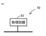
- FIG. 4 is a hardware configuration diagram of another example of the vehicle control device according to Embodiment 1.
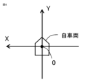
- FIG. FIG. 2 is a diagram illustrating a coordinate system of own vehicle according to Embodiment 1;
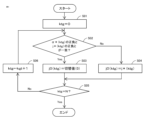
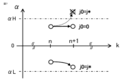
- FIG. FIG. 4 is a diagram illustrating setting of a constraint condition of acceleration and an initial value of jerk according to Embodiment 1; 4 is a flowchart for explaining setting of an initial value of jerk according to Embodiment 1.
- FIG. 10 is a diagram illustrating setting of a constraint condition of acceleration and an initial value of jerk according to Embodiment 2; 9 is a flow chart for explaining setting of an initial value of jerk according to Embodiment 2.
- FIG. 11 is a flowchart for explaining setting of an initial value of jerk according to Embodiment 3.
- Embodiment 1 An optimum arithmetic device according to Embodiment 1 will be described with reference to the drawings.
- the optimum calculation device is mounted on the own vehicle and performs optimum calculation for the control of the own vehicle.
- the optimum computing device is incorporated in the vehicle control device 50 .
- the vehicle system 1 and the vehicle control device 50 are mounted on the own vehicle.
- the vehicle system 1 includes a vehicle state detection device 31, a surroundings monitoring device 32, a position detection device 33, a map information database 34, a wireless communication device 35, a vehicle control device 50, a drive control device 36, and a power machine 8. , and the electric steering device 7 and the like.
- the vehicle state detection device 31 is a detection device that detects the running state of the own vehicle.
- the vehicle speed V, acceleration ⁇ , roll angular velocity, pitch angular velocity, and yaw angular velocity ⁇ of the own vehicle are detected as the running state of the own vehicle.
- the vehicle state detection device 31 is provided with a three-axis angular velocity sensor for detecting roll angular velocity, pitch angular velocity, and yaw angular velocity acting on the vehicle, an acceleration sensor, and a speed sensor for detecting wheel rotation speed.
- the speed of the own vehicle may be detected by other methods such as integrating acceleration.
- the perimeter monitoring device 32 is a device such as a camera or radar that monitors the perimeter of the vehicle.
- a millimeter wave radar, a laser radar, an ultrasonic radar, or the like is used as the radar.
- the wireless communication device 35 performs wireless communication with a base station using a cellular wireless communication standard such as 4G or 5G.
- the position detection device 33 is a device that detects the current position (latitude, longitude, altitude) of the own vehicle, and a GPS antenna or the like that receives signals output from artificial satellites such as GNSS (Global Navigation Satellite System) is used. .
- GNSS Global Navigation Satellite System
- Various methods are used to detect the current position of the own vehicle, such as a method using the lane number of the own vehicle, a map matching method, a dead reckoning method, and a method using detection information about the surroundings of the own vehicle. may
- the map information database 34 stores road information such as road shape (eg, road position, number of lanes, shape of each lane, road type, speed limit, etc.), signs, and signals.
- the map information database 34 is mainly composed of a storage device. Note that the map information database 34 may be provided in a server outside the vehicle connected to the network, and the vehicle control device 50 acquires necessary road information from the server outside the vehicle via the wireless communication device 35. good too.
- the drive control device 36 includes a power control device, a brake control device, an automatic steering control device, a light control device, and the like.
- the power control device controls the output of a power machine 8 such as an internal combustion engine and a motor.
- the brake control device controls the braking operation of the electric brake device.
- the automatic steering control device controls the electric steering device 7 .
- the light controller controls direction indicators, hazard lamps and the like.
- Vehicle control device 50 The vehicle control device 50 includes functional units such as a peripheral situation acquisition unit 51, a running state acquisition unit 52, a target running state setting unit 53, an initial value setting unit 54, an optimum value calculation unit 55, and a vehicle control unit 56. . Each function of the vehicle control device 50 is implemented by a processing circuit included in the vehicle control device 50 . Specifically, as shown in FIG. 2, the vehicle control device 50 includes an arithmetic processing unit 90 such as a CPU (Central Processing Unit), a storage device 91, and an input/output device for inputting/outputting external signals to the arithmetic processing unit 90. 92 and so on.
- arithmetic processing unit 90 such as a CPU (Central Processing Unit)
- storage device 91 a storage device 91
- input/output device for inputting/outputting external signals to the arithmetic processing unit 90. 92 and so on.
- ASIC Application Specific Integrated Circuit
- IC Integrated Circuit
- DSP Digital Signal Processor
- FPGA Field Programmable Gate Array
- GPU Graphics Processing Unit
- AI Artificial Intelligence
- RAM Random Access Memory
- ROM Read Only Memory
- flash memory EEPROM (Electrically Erasable Programmable Read Only Memory)
- hard disk and DVD device
- the input/output device 92 includes a communication device, an A/D converter, an input/output port, a drive circuit, and the like.
- the input/output device 92 is connected to the vehicle state detection device 31, the surroundings monitoring device 32, the position detection device 33, the map information database 34, the wireless communication device 35, the drive control device 36, etc., and communicates with these devices.
- Each function of the functional units 51 to 56 provided in the vehicle control device 50 is executed by the arithmetic processing device 90 by executing software (programs) stored in the storage device 91, the storage device 91, the input/output device 92 and the like. It is realized by cooperating with other hardware of the vehicle control device 50 of .
- Setting data such as determination values used by the functional units 51 to 56 and the like are stored in a storage device 91 such as an EEPROM as a part of software (program).
- the vehicle control device 50 may include, as a processing circuit, dedicated hardware 93 such as a single circuit, multiple circuits, programmed processor, parallel programmed processor, ASIC, FPGA, as shown in FIG. , GPU, AI chip, or a circuit combining these may be provided. Each function of the vehicle control device 50 will be described in detail below.
- Peripheral situation acquisition unit 51 acquires the peripheral situation of the own vehicle. For example, the peripheral situation acquisition unit 51 detects other vehicles and the like existing around the own vehicle. The peripheral situation acquisition unit 51 detects the position, moving direction, moving speed, and the like of other vehicles based on the detection information acquired from the peripheral monitoring device 32 and the position information of the own vehicle acquired from the position detection device 33 . In addition to other vehicles, the surrounding situation acquisition unit 51 also detects lane shapes such as road division lines, obstacles, pedestrians, signs, and the like.
- Running state acquisition unit 52 The running state acquisition unit 52 acquires the running state of the own vehicle.
- the running state acquisition unit 52 acquires the vehicle speed V, the acceleration ⁇ , the roll angular velocity, the pitch angular velocity, and the yaw angular velocity ⁇ of the own vehicle as the running state of the own vehicle from the vehicle state detection device 31 .
- the running state acquisition unit 52 acquires the position, moving direction, etc. of the own vehicle based on the position information of the own vehicle acquired from the position detection device 33 .
- the traveling state acquiring unit 52 acquires information on the traveling position of the host vehicle with respect to the lane based on the shape of the lane acquired from the surrounding situation acquiring unit 51 .
- the driving state acquisition unit 52 acquires the driving operation state such as the steering angle ⁇ , the output of the power machine such as the internal combustion engine, and the operation state of the brake from the vehicle control unit 56 .
- Target running state setting unit 53 The target running state setting unit 53 sets the target running state of the own vehicle.
- the target running state setting unit 53 generates a target running state in accordance with the conditions of other vehicles, road shapes, obstacles, pedestrians, and the like around the own vehicle detected by the surrounding situation acquisition unit 51 .
- the target travel state is a target travel trajectory, and is a time-series travel plan including the position of the vehicle, the traveling direction of the vehicle, and the speed of the vehicle at each point in the future.
- Various known methods are used to generate the target travel trajectory.
- Vehicle control unit 56 The vehicle control unit 56 controls the own vehicle based on the target value of the vehicle control amount set by the optimum value calculation unit 55, which will be described later.
- the target value of the vehicle control amount is the target value of the steering angle ⁇ at each time point and the target value of the acceleration ⁇ at each time point.
- the vehicle control unit 56 outputs a command value to the power control device, a command value to the brake control device, and a command value to the automatic steering control device based on the target value of the steering angle ⁇ at each time point and the acceleration ⁇ at each time point. is calculated and transmitted to each device.
- the power control device controls the output of power machines such as internal combustion engines and motors according to command values.
- the brake control device controls the braking operation of the electric brake device according to the command value.
- the automatic steering control device controls the electric steering device according to the command value.
- Initial value setting unit 54 and optimum value calculation unit 55 The initial value setting unit 54 sets an initial value u0(k) of the input variable u(k) at each point k in the prediction period.
- the optimum value calculation unit 55 uses a state equation for calculating the state variable x with the input variable u as an input so as to solve an optimization problem having two or more evaluation factors in each calculation cycle, and calculates the input variable u as The initial value u0 is updated by iterative calculation, and the optimum value u*(0) of the input variable at each point k in the prediction period is calculated.
- the state equation of the state variable x is such that the time derivative dx/dt(k) of the state variable at each time point k is the state variable x(k) and the input variable u(k) at each time point k. It is represented by a function f as an input. If there are multiple state variables, x will be a vector, and if there are multiple input variables, u will be a vector.
- the state variable x(k+1) at the next point in time is the state variable x(k) at the present point in time, the time derivative dx(k)/dt of the state variable at the present point in time, and the time between points in the prediction period It is calculated by adding the value multiplied by the interval ⁇ T.
- the input variable u(k) at each time point k (k 0, . While incrementing the time point k from 0 to N one by one, based on the input variable u(k) and the state variable x(k) at the current time point k, using equations (1) and (2), the following
- the state variables x(k+1) at time k+1 are calculated in turn.
- J is an evaluation function that evaluates the state variable x(k) and the input variable u(k), and is the first evaluation element.
- the evaluation function J is a quadratic expression.
- g is a constraint that constrains the state variable x(k) and the input variable u(k), has a set number O of constraints, and is the second and subsequent evaluation elements.
- the optimization problem is to divide the gradients of two or more evaluation factors by the Lagrangian multiplier ⁇ . It has the Karush-Kuhn-Tucker condition (KKT condition), which is the optimal condition that the optimal value should satisfy, which is linearly combined.
- KT condition Karush-Kuhn-Tucker condition
- ⁇ is an operator that performs partial differentiation at the operating point and calculates the gradient.
- x* is the optimal value of the state variable and u* is the optimal value of the input variable.
- ⁇ i are Lagrangian multipliers that linearly combine the gradient of each constraint gi with the gradient of the evaluation function J. If the state variable x and the input variable u are optimal values, there exists a value for each Lagrangian multiplier ⁇ i that satisfies all equations (4) through (7).
- a known technique such as the active constraint method for calculating the optimum value that satisfies the KKT condition is used.
- the constraint g that the Lagrangian multiplier ⁇ becomes negative does not constrain the optimum value. Therefore, it is determined that the constraint g is invalid.
- the state variable x* and the input Create a variable u*. The generation of the state variable x* and the input variable u* is repeated until there are no more negative Lagrangian multipliers ⁇ . Constraint g exceptions are made one by one.
- the initial value setting unit 54 performs the initial calculation using the initial value u0 of the input variable in the optimum value calculation unit 55, from the optimization problem, the evaluation element of the target type (this example Then, switch between multiple setting methods to set the initial value of a specific type of input variable so that the constraint condition can be excluded.
- the optimum value calculation unit 55 excludes the target type evaluation element (constraint condition in this example) related to the specific type of input variable from the optimization problem, perform calculations.
- the initial value of the specific type of input variable is set by switching between a plurality of setting methods so as to exclude the target type constraint condition related to the specific type of input variable.
- the calculations can be performed by removing the target type constraints from the optimization problem, thus reducing the calculation processing load.
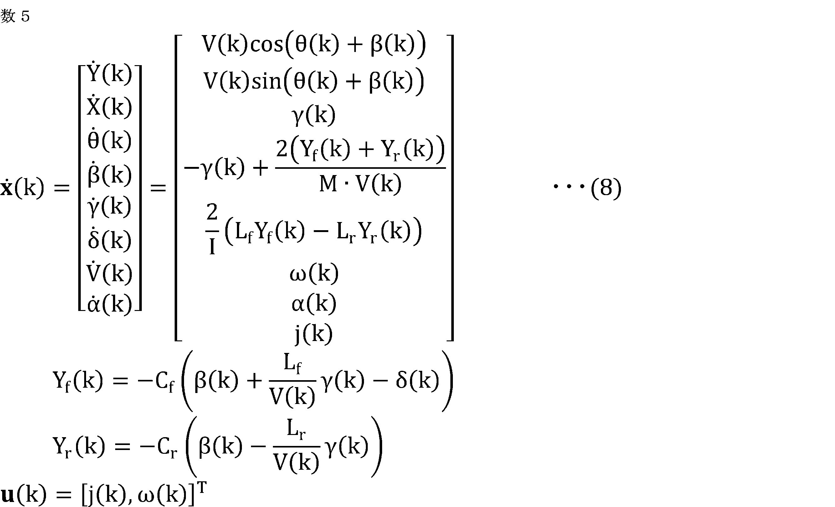
- ⁇ Vehicle model> a state equation of a vehicle model is used in which an input variable u related to vehicle control is input and a state variable x representing the behavior of the own vehicle is calculated.
- a two-wheel model is used as the vehicle model.
- the state equation of the vehicle model is represented by a differential equation of each state variable representing the behavior of the own vehicle, as shown in the following equation.
- Various well-known state equations may be used as the state equation of the vehicle model.
- the dot sign above each variable on the left side indicates that it is the time differential value of each state variable.
- state variable x indicates the position of the vehicle in the longitudinal direction
- X indicates the position of the vehicle in the lateral direction
- ⁇ is the inclination of the vehicle in the longitudinal direction
- ⁇ is the tilt of the vehicle.
- ⁇ is the sideslip angle of the center of gravity
- ⁇ is the yaw angular velocity of the own vehicle
- ⁇ is the steering angle of the wheels of the own vehicle
- V is the speed of the own vehicle
- ⁇ is the acceleration of the own vehicle.
- j is the jerk of the own vehicle
- ⁇ is the steering angular velocity of the own vehicle
- I is the yaw moment of inertia of the vehicle
- M is the mass of the vehicle
- Lf is the distance between the vehicle center of gravity and the front axle
- Lr is the distance between the vehicle center of gravity and the rear axle.
- Yf is the front wheel cornering force
- Yr is the rear wheel cornering force
- Cf is the front tire cornering stiffness
- Cr is the rear tire cornering stiffness.
- the state equation is expressed in the coordinate system X, Y of the own vehicle based on the current position of the own vehicle. As shown in FIG. 4, X is the lateral direction of the vehicle, and Y is the longitudinal direction of the vehicle. A coordinate system based on the target travel trajectory may be used instead of the coordinate system of the own vehicle.
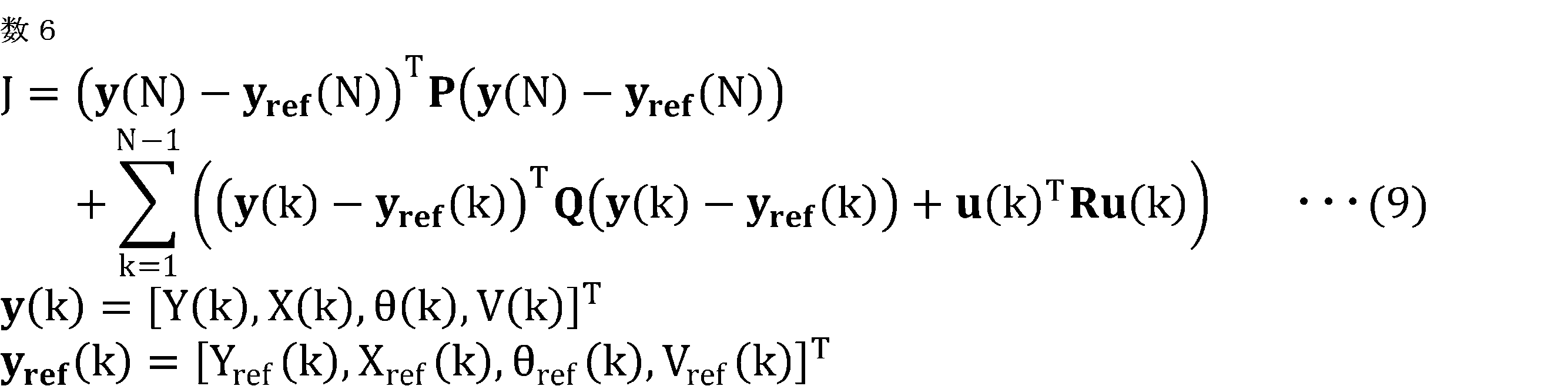
- the evaluation function J is an evaluation element whose evaluation increases (in this example, the value decreases) as the difference between the target running state (target running trajectory) and the predicted running state decreases. Note that the evaluation function J may be modified from the formula (9).
- the instant number k is incremented by one from 0 to N every time interval ⁇ T. Therefore, k ⁇ T is the elapsed time from the present at each time point k.
- y(k) is the vector of output variables of the state equation at each instant k.
- yref(k) is a vector of the target values of the output variables at each time point k, and the value of the target travel trajectory at each time point k is set.
- the term of this weight R is used to evaluate so that the jerk j and the steering angular velocity ⁇ of the own vehicle do not become too large. Therefore, by setting the respective weights P, Q, and R, the variation in the steering angle and the vehicle acceleration are balanced with the followability to the target travel trajectory, and the vehicle control is performed with little sense of discomfort for the driver.
- the target value of the vehicle control amount at each time point k is the steering angle ⁇ *(k) and the acceleration ⁇ *( k).
- the acceleration ⁇ is limited by a positive upper limit value ⁇ H and a negative lower limit value ⁇ L as shown in the following equations. . This is to improve the comfort of the ride.
- the horizontal position X is upper-limited by a positive upper-limit value XH and lower-limited by a negative lower-limit value XL, as shown in the following equations. This is to prevent deviation from the planned travel range.
- the upper limit value XH and the lower limit value XL at each time point may be changed according to the target travel trajectory at each time point.
- the initial value setting unit 54 in the initial calculation using the initial value u0 of the input variable in the optimum value calculation unit 55, from the optimization problem, the constraint condition of the target type related to the specific type of input variable Switch between multiple configuration schemes to set initial values for certain types of input variables so that
- the first particular type of input variable is set to jerk j
- the first target type evaluation factor associated with the first particular type of input variable is Equation (10) are set to the first and second constraints g1 and g2 shown in FIG.
- the initial value setting unit 54 can exclude the first and second constraints g1 and g2 related to the jerk j from the optimization problem in the initial calculation using the jerk initial value j0. , the initial value j0 of the jerk is set by switching among a plurality of setting methods.
- the initial value setting unit 54 sets the initial value j0 ( k). where ⁇ (0) is set to the current detected value.
- the optimum value calculator 55 applies the first and second constraints g1.
- the Lagrangian multipliers ⁇ 1, ⁇ 2 of g2 can be set to 0 to reduce the number of valid constraints initially set. Therefore, the calculation processing load of the optimum value calculator 55 can be reduced.
- the first and second constraints g1 and g2 are the state variables acceleration This is an evaluation element for upper limiting ⁇ (state variable of specific influence) with a positive upper limit value ⁇ H and lower limit with a negative lower limit value ⁇ L.
- the initial value setting unit 54 determines whether the optimum value j* of the jerk calculated in the previous calculation cycle is positive or negative, and the optimum value ⁇ * of the acceleration calculated in the previous calculation cycle is positive or negative. It is determined whether or not they match, and the initial value j0 of the jerk is set by switching between a plurality of setting methods depending on whether or not the two signs match.
- the acceleration ⁇ (k) at a certain time point k is positive and the jerk j(k) is positive
- the acceleration ⁇ (k+1) at the next time point k+1 is the upper limit value.
- the acceleration ⁇ (k+1) at the next time point k+1 is the upper limit value.
- the acceleration ⁇ (k+1) at the next time point k+1 approaches the lower limit value ⁇ L. may be constrained by the constraint g2 of .
- the initial You can set the value.
- the initial value setting unit 54 sets the initial value j0 of the jerk to the optimum value j* of the jerk calculated in the previous calculation cycle when the two signs do not match.
- the initial value setting unit 54 uses a setting method of setting the initial value j0 of the jerk to a switching value such that the acceleration ⁇ does not exceed the upper limit value ⁇ H or the lower limit value ⁇ L when the two positive and negative values match. .
- the switching value is set so as not to exceed the upper limit value ⁇ H or the lower limit value ⁇ L, thereby preventing the acceleration ⁇ from exceeding the upper limit value ⁇ H or the lower limit value ⁇ L. can.
- the initial value setting unit 54 uses 0 as the switching value.
- the initial value j0 of the jerk is set to 0 when the two positive and negative values match, so the acceleration ⁇ does not increase or decrease and is kept at a constant value. Therefore, the acceleration ⁇ can be prevented from approaching the upper limit value ⁇ H or the lower limit value ⁇ L, and the acceleration ⁇ can be prevented from exceeding the upper limit value ⁇ H or the lower limit value ⁇ L.
- a value other than 0 may be used as the switching value.
- the initial value setting unit 54 may set the switching value based on a value corresponding to the upper limit value ⁇ H or the lower limit value ⁇ L. For example, the initial value setting unit 54 switches the value obtained by multiplying the optimum value of the previous calculation cycle by a coefficient set according to the deviation (margin) between the upper limit value ⁇ H or the lower limit value ⁇ L on the approaching side and the acceleration ⁇ . May be set as a value. As the deviation (margin) becomes smaller, the coefficient is made smaller than 1, and when the deviation (margin) becomes 0, the coefficient is set to 0.
- the initial value setting unit 54 performs the above setting for the initial value j0(k) of the jerk at each time point k.
- step S01 the time ktg to be processed is set to zero.
- step S02 the initial value setting unit 54 determines whether the optimum value ⁇ *(ktg) of the acceleration at the time point ktg of the processing target calculated in the previous calculation cycle is positive or negative, and the processing target calculated in the previous calculation cycle. It is determined whether the positive and negative of the optimum value j*(ktg) of the jerk at the time point ktg match. If not, proceed to step S04.
- step S03 the initial value setting unit 54 sets the initial value j0 (ktg) of the jerk at time ktg to be processed to a switching value (in this example, 0).
- step S04 the initial value setting unit 54 sets the initial value j0 (ktg) of the jerk at time ktg to be processed to the optimal value j of the jerk at time ktg to be processed calculated in the previous calculation cycle. * Set to (ktg).
- step S05 the initial value setting unit 54 determines whether or not the time point ktg to be processed is the final time point N. After incrementing it by 1, the process returns to step S02, and if it is the final time point N, the process ends.
- a second specific type of input variable is set to the steering angular velocity ⁇ , and a second target type of evaluation factor associated with the second specific type of input variable is the third and It is set in the fourth constraints g3 and g4.
- the initial value setting unit 54 can exclude the third and fourth constraints g3 and g4 related to the steering angular velocity ⁇ from the optimization problem in the initial calculation using the initial value ⁇ 0 of the steering angular velocity.
- the initial value ⁇ 0 of the steering angular velocity is set by switching among a plurality of setting methods.
- the initial value setting unit 54 sets the initial value of the steering angular velocity at each time so that the lateral position X(k) at each time is not limited by the positive upper limit value XH and is not limited by the negative lower limit value XL. Set the value ⁇ 0(k).
- the optimum value calculator 55 applies the third and fourth constraints g3,
- the Lagrangian multipliers ⁇ 3, ⁇ 4 of g4 can be set to 0 to reduce the number of valid constraints initially set. Therefore, the calculation processing load of the optimum value calculator 55 can be reduced.
- the third and fourth constraints g3 and g4 are the state variables that change according to the steering angular velocity ⁇ (input variable of a specific type). It is an evaluation factor for upper limiting the direction position X (state variable of specific influence) with a positive upper limit value XH and lower limit with a negative lower limit value XL.
- the initial value setting unit 54 determines whether the optimum value ⁇ * of the steering angular velocity calculated in the previous calculation cycle is positive or negative, and the optimum value X* of the lateral position calculated in the previous calculation cycle.
- the initial value ⁇ 0 of the steering angular velocity is set by switching between a plurality of setting methods depending on whether the two positive and negative values match.
- the lateral position X(k) at a certain time point k is positive and the steering angular velocity ⁇ (k) is positive
- the lateral position X(k) at the next time point k+1 k+1) approaches the upper bound XH and may be constrained by the third constraint g3.
- the lateral position X(k) at a certain time point k is negative and the steering angular velocity ⁇ (k) is negative
- the lateral position X(k+1) at the next time point k+1 is the lower limit.
- XL and may be constrained by the fourth constraint g4.
- the initial value can be effectively set by switching the setting method and setting the initial value depending on whether the two positive and negative values match.
- the initial value setting unit 54 sets the initial value ⁇ 0 of the steering angular velocity to the optimal value ⁇ * of the steering angular velocity calculated in the previous calculation cycle when the two signs do not match.
- the initial value setting unit 54 sets the initial value ⁇ 0 of the steering angular velocity to a switching value such that the position X in the lateral direction does not exceed the upper limit value XH or the lower limit value XL when the two positive and negative values match. method.
- the horizontal position X exceeds the upper limit value XH or the lower limit value XL by setting the switching value so as not to exceed the upper limit value XH or the lower limit value XL. You can avoid it.
- the initial value setting unit 54 uses 0 as the switching value.
- the initial value ⁇ 0 of the steering angular velocity is set to 0 when the two positive and negative values match, so the position X in the lateral direction does not increase or decrease significantly. Therefore, the lateral position X can be prevented from approaching the upper limit value XH or the lower limit value XL, and the lateral position X can be prevented from exceeding the upper limit value XH or the lower limit value XL.
- the initial value setting unit 54 may set the switching value based on a value corresponding to the upper limit value XH or the lower limit value XL. For example, the initial value setting unit 54 multiplies the optimal value of the previous calculation cycle by a coefficient set according to the deviation (margin) between the upper limit value XH or the lower limit value XL on the approaching side and the position X in the lateral direction. may be set as the switching value. As the deviation (margin) becomes smaller, the coefficient is made smaller than 1, and when the deviation (margin) becomes 0, the coefficient is set to 0.
- the initial value setting unit 54 performs the above setting for the initial value ⁇ 0(k) of the steering angular velocity at each time point k. Since the setting process of the initial value ⁇ 0 of the steering angular velocity is the same as that of the initial value j0 of the jerk shown in the flowchart of FIG. 6, the description thereof will be omitted.
- Embodiment 2 Next, an optimum arithmetic device according to Embodiment 2 will be described. Descriptions of the same components as in the first embodiment are omitted.
- the basic configuration of the optimum arithmetic unit according to this embodiment is the same as that of the first embodiment, but the processing of the initial value setting unit 54 is different from that of the first embodiment.
- the initial value setting unit 54 in the initial calculation using the initial value u0 of the input variable in the optimum value calculation unit 55, from the optimization problem, the target type constraint related to the specific type of input variable Toggle between multiple configuration schemes to set initial values for certain types of input variables so that conditions can be ruled out.
- the first specific type of input variable is set to the jerk j
- the first target type evaluation factor associated with the first specific type of input variable is given by equation (10) are set to the first and second constraints g1 and g2 shown in FIG.
- the first and second constraints g1 and g2 (evaluation elements of the target type) set the acceleration ⁇ (state variable of specific influence), which is a state variable that changes according to the jerk j (input variable of a specific type), It is an evaluation factor for limiting the upper limit with a positive upper limit value ⁇ H and limiting the lower limit with a negative lower limit value ⁇ L.
- the acceleration ⁇ is set to the upper limit value ⁇ H or It is determined whether or not the lower limit value ⁇ L is exceeded, and the initial value j0 of the jerk is set by switching between a plurality of setting methods depending on whether or not the lower limit value ⁇ L is exceeded.
- the initial value j0 of the jerk when the initial value j0 of the jerk is set to the optimum value j* of the jerk in the previous calculation cycle, if the acceleration ⁇ exceeds the upper limit value ⁇ H or the lower limit value ⁇ L, By switching the setting method and setting the initial value j0 of the jerk, the initial value can be set so that the acceleration ⁇ does not exceed the upper limit value ⁇ H or the lower limit value ⁇ L.
- the initial value setting unit 54 determines that the acceleration ⁇ does not exceed the upper limit value ⁇ H or the lower limit value ⁇ L
- the initial value j0 of the jerk is set to the jerk calculated in the previous calculation cycle. is set to the optimal value j*.
- the optimum value of the previous calculation period is set as the initial value, thereby reducing the calculation processing load for searching for the optimum value.
- the initial value setting unit 54 sets the initial value j0 of the jerk to a value such that the acceleration ⁇ does not exceed the upper limit value ⁇ H or the lower limit value ⁇ L.
- a setting method that sets the switching value is used.
- the switching value is set so that the acceleration ⁇ does not exceed the upper limit value ⁇ H or the lower limit value ⁇ L.
- the initial value setting unit 54 uses 0 as the switching value.
- the initial value j0 of the jerk is set to 0 when it is determined that it exceeds, so the acceleration ⁇ is kept at a constant value without increasing or decreasing. Therefore, the acceleration ⁇ can be prevented from exceeding the upper limit value ⁇ H or the lower limit value ⁇ L.
- the initial value setting unit 54 may set the switching value based on a value corresponding to the upper limit value ⁇ H or the lower limit value ⁇ L. For example, the initial value setting unit 54 may set, as the switching value, a predetermined value having positive and negative signs opposite to those of the exceeded upper limit value ⁇ H or lower limit value ⁇ L.
- the upper limit value ⁇ H used for determination a value smaller than the upper limit value ⁇ H by a predetermined value may be used, and as the lower limit value ⁇ L used for determination, a value greater than the lower limit value ⁇ L by a predetermined value is used. may It is possible to set the initial value j0 of the jerk by giving a margin to the acceleration ⁇ with respect to the upper limit value ⁇ H or the lower limit value ⁇ L.
- the initial value setting unit 54 increments the time point k from 0 to N by one, and at each time point, sets the initial value j0 of the jerk already set before that time point, and Using the optimal value j* of the jerk as the initial value, calculate the acceleration ⁇ up to the next time in order, and determine whether the acceleration ⁇ at the next time exceeds the upper limit value ⁇ H or the lower limit value ⁇ L judge. If the initial value setting unit 54 determines that it does not exceed, it sets the initial value j0 of the jerk at that time to the optimal value j* of the jerk at that time in the previous calculation cycle, and determines that it exceeds If so, the initial value j0 of the jerk at that time is set as the switching value.
- step S11 the time ktg to be processed is set to zero.
- step S12 the initial value setting unit 54 sets the initial values j0(0) to j0(ktg-1) of the jerk already set before the time ktg to be processed, and Using the optimum value j*(ktg) of the jerk at time ktg as the initial value j0(ktg) at time ktg to be processed, using equation (12), the acceleration ⁇ (ktg+1) up to the next time ktg+1 to be processed are calculated in order. Then, the initial value setting unit 54 determines whether or not the acceleration ⁇ (ktg+1) to be processed at the next point in time exceeds the upper limit value ⁇ H or falls below the lower limit value ⁇ L. If so, the process proceeds to step S13; otherwise, the process proceeds to step S14.
- step S13 the initial value setting unit 54 sets the initial value j0 (ktg) of the jerk at time ktg to be processed, and the acceleration ⁇ (ktg+1) at the next time to be processed exceeds the upper limit value ⁇ H or the lower limit value ⁇ L.
- a switching value (0 in this example) is set so that it does not occur.
- step S14 the initial value setting unit 54 sets the initial value j0 (ktg) of the jerk at time ktg to be processed to the optimal value j of the jerk at time ktg to be processed calculated in the previous calculation cycle. * Set to (ktg).
- step S15 the initial value setting unit 54 determines whether or not the time point ktg to be processed is the final time point N. After incrementing it by 1, the process returns to step S12, and if it is the final time point N, the process ends.
- a second specific type of input variable is set to the steering angular velocity ⁇
- a second target type of evaluation factor associated with the second specific type of input variable is the third and It is set in the fourth constraints g3 and g4.
- the third and fourth constraints g3 and g4 are lateral position X (specific effect state variable ) is upper bounded by a positive upper limit value XH and lower bounded by a negative lower limit value XL.
- the initial value setting unit 54 sets the initial value ⁇ 0 of the steering angular velocity to the optimal value ⁇ * of the steering angular velocity calculated in the previous calculation cycle, and the lateral position X is the upper limit. It is determined whether or not the value XH or the lower limit value XL is exceeded, and a plurality of setting methods are switched depending on whether or not the initial value ⁇ 0 of the steering angular velocity is set.
- the setting method is switched and the initial value ⁇ 0 of the steering angular velocity is set so that the lateral position X becomes the upper limit.
- the initial value can be set so that the value XH or the lower limit XL is not exceeded.
- the initial value setting unit 54 determines that the lateral position X does not exceed the upper limit value XH or the lower limit value XL
- the initial value ⁇ 0 of the steering angular velocity is calculated in the previous calculation cycle. is set to the optimum value ⁇ * of the steering angular velocity.
- the optimum value of the previous calculation period is set as the initial value, thereby reducing the calculation processing load for searching for the optimum value.
- the initial value setting unit 54 sets the initial value ⁇ 0 of the steering angular velocity to A setting method that sets a switching value that does not exceed XL is used.
- the switching value is set so that the lateral position X does not exceed the upper limit value XH or the lower limit value XL. can be done.
- the initial value setting unit 54 uses 0 as the switching value.
- the initial value ⁇ 0 of the steering angular velocity is set to 0 when it is determined that it exceeds, so the position X in the lateral direction does not greatly increase or decrease. Therefore, it is possible to prevent the horizontal position X from exceeding the upper limit value XH or the lower limit value XL.
- the initial value setting unit 54 may set the switching value based on a value corresponding to the upper limit value XH or the lower limit value XL. For example, the initial value setting unit 54 may set, as the switching value, a predetermined value having positive and negative signs opposite to those of the exceeded upper limit value XH or lower limit value XL.
- the upper limit value XH used for determination a value smaller than the upper limit value XH by a predetermined value may be used, and as the lower limit value XL used for determination, a value greater than the lower limit value XL by a predetermined value may be used.
- the initial value ⁇ 0 of the steering angular velocity can be set with a margin in the lateral position X relative to the upper limit value XH or the lower limit value XL.
- the initial values of the other input variables at each time point (in this example, the initial value j0 of the jerk) are values set so as not to exceed the optimum value, upper limit value, or lower limit value of the previous calculation cycle. Used.
- the initial value setting unit 54 determines whether the horizontal position X at the next time exceeds the upper limit value XH or the lower limit value XL. If the initial value setting unit 54 determines that it does not exceed the initial value ⁇ 0 of the steering angular velocity at that time, it sets the initial value ⁇ 0 of the steering angular velocity at that time to the optimal value ⁇ * of the steering angular velocity at that time in the previous calculation cycle. sets the initial value ⁇ 0 of the steering angular velocity at that time as the switching value.
- the processing for setting the initial value ⁇ 0 of the steering angular velocity is the same as that for the initial value j0 of the jerk shown in the flowchart of FIG. 8, so the description is omitted.
- Embodiment 3 Next, an optimum arithmetic device according to Embodiment 3 will be described. Descriptions of components similar to those in the first or second embodiment are omitted.
- the basic configuration of the optimum arithmetic unit according to this embodiment is the same as that of the first or second embodiment, but the processing of the initial value setting unit 54 is different from that of the first or second embodiment.
- the initial value setting unit 54 in the initial calculation using the initial value u0 of the input variable in the optimum value calculation unit 55, from the optimization problem, the target type constraint related to the specific type of input variable Toggle between multiple configuration schemes to set initial values for certain types of input variables so that conditions can be ruled out.
- the first specific type of input variable is set to the jerk j
- the first target type evaluation factor associated with the first specific type of input variable is given by equation (10) are set to the first and second constraints g1 and g2 shown in FIG.
- the first and second constraints g1 and g2 (evaluation elements of the target type) set the acceleration ⁇ (state variable of specific influence), which is a state variable that changes according to the jerk j (input variable of a specific type), It is an evaluation factor for limiting the upper limit with a positive upper limit value ⁇ H and limiting the lower limit with a negative lower limit value ⁇ L.
- the initial value setting unit 54 sets the sign of the optimum value j* of the jerk calculated in the previous calculation cycle and the sign of the optimum value ⁇ * of the acceleration calculated in the previous calculation cycle. It is determined whether or not they match.
- the initial value setting unit 54 sets the initial value j0 of the jerk to the optimal value j* of the jerk calculated in the previous calculation cycle when the two signs do not match. Use the setting method.
- the initial value setting unit 54 sets the initial value j0 of the jerk to It is determined whether or not the acceleration ⁇ exceeds the upper limit value ⁇ H or the lower limit value ⁇ L when the optimum value j* of the jerk is set.
- the initial value setting unit 54 determines that the acceleration ⁇ does not exceed the upper limit value ⁇ H or the lower limit value ⁇ L, the initial value j0 of the jerk is set to the optimal value j of the jerk calculated in the previous calculation cycle. Use the setting method to set to *.
- the initial value setting unit 54 sets the initial value j0 of the jerk to a value such that the acceleration ⁇ does not exceed the upper limit value ⁇ H or the lower limit value ⁇ L.
- a setting method that sets the switching value is used.
- acceleration ⁇ when the two signs are the same and there is a possibility that the acceleration ⁇ exceeds the upper limit value ⁇ H or the lower limit value ⁇ L, the acceleration ⁇ actually exceeds the upper limit value ⁇ H or the lower limit value ⁇ L. Acceleration ⁇ can be prevented from exceeding the upper limit value ⁇ H or the lower limit value ⁇ L by setting a switch value that does not exceed the upper limit value ⁇ H or the lower limit value ⁇ L when it exceeds. If it is determined that it does not actually exceed, the optimum value of the previous calculation cycle is set as the initial value. Therefore, when the two positive and negative values match, it is possible to make a stepwise determination and set the initial value more appropriately.
- the initial value setting unit 54 uses 0 as the switching value.
- the initial value j0 of the jerk is set to 0 when it is determined that it exceeds, so the acceleration ⁇ is kept at a constant value without increasing or decreasing. Therefore, the acceleration ⁇ can be prevented from exceeding the upper limit value ⁇ H or the lower limit value ⁇ L.
- the initial value setting unit 54 may set the switching value based on a value corresponding to the upper limit value ⁇ H or the lower limit value ⁇ L. For example, the initial value setting unit 54 may set, as the switching value, a predetermined value having positive and negative signs opposite to those of the exceeded upper limit value ⁇ H or lower limit value ⁇ L.
- the upper limit value ⁇ H used for determination a value smaller than the upper limit value ⁇ H by a predetermined value may be used, and as the lower limit value ⁇ L used for determination, a value greater than the lower limit value ⁇ L by a predetermined value is used. may It is possible to set the initial value j0 of the jerk by giving a margin to the acceleration ⁇ with respect to the upper limit value ⁇ H or the lower limit value ⁇ L.
- the initial value setting unit 54 increments the time point k from 0 to N by one, and determines whether or not the two positive and negative values match at each time point.
- the initial value j0 of the jerk at that time is set to the optimum value j* of the jerk at that time in the previous calculation cycle.
- the initial value setting unit 54 sets the initial value j0 of the jerk set before that time and the optimal value of the jerk at that time in the previous calculation cycle.
- j* as an initial value, the acceleration ⁇ up to the next point in time is calculated in order, and it is determined whether or not the acceleration ⁇ at the next point in time exceeds the upper limit value ⁇ H or the lower limit value ⁇ L.
- the initial value setting unit 54 determines that it does not exceed, it sets the initial value j0 of the jerk at that time to the optimal value j* of the jerk at that time in the previous calculation cycle, and determines that it exceeds If so, the initial value j0 of the jerk at that time is set as the switching value.
- step S21 the time ktg to be processed is set to zero. Then, in step S22, the initial value setting unit 54 determines whether the optimum value ⁇ *(ktg) of the acceleration at the time point ktg of the processing target calculated in the previous calculation cycle is positive or negative, and the processing target calculated in the previous calculation cycle. It is determined whether the positive and negative of the optimum value j*(ktg) of the jerk at the time point ktg match. If not, proceed to step S25.
- step S23 the initial value setting unit 54 sets the initial values j0(0) to j0(ktg-1) of the jerk already set before the time ktg to be processed, and Using the optimum value j*(ktg) of the jerk at time ktg as the initial value j0(ktg) at time ktg to be processed, using equation (12), the acceleration ⁇ (ktg+1) up to the next time ktg+1 to be processed are calculated in order. Then, the initial value setting unit 54 determines whether or not the acceleration ⁇ (ktg+1) to be processed at the next point in time exceeds the upper limit value ⁇ H or falls below the lower limit value ⁇ L. If it is, the process proceeds to step S24, and if it is neither higher nor lower, the process proceeds to step S25.
- step S24 the initial value setting unit 54 sets the initial value j0 (ktg) of the jerk at time point ktg to be processed, and the acceleration ⁇ (ktg+1) at the next time point to be processed exceeds the upper limit value ⁇ H or the lower limit value ⁇ L.
- a switching value (0 in this example) is set so that it does not occur.
- step S25 the initial value setting unit 54 sets the initial value j0 (ktg) of the jerk at time ktg to be processed to the optimal value j of the jerk at time ktg to be processed calculated in the previous calculation cycle. * Set to (ktg).
- step S26 the initial value setting unit 54 determines whether or not the time point ktg to be processed is the final time point N. After incrementing by one, the process returns to step S22, and if the final time point N is reached, the process ends.
- a second specific type of input variable is set to the steering angular velocity ⁇
- a second target type of evaluation factor associated with the second specific type of input variable is the third and It is set in the fourth constraints g3 and g4.
- the third and fourth constraints g3 and g4 are lateral position X (specific effect state variable ) is upper bounded by a positive upper limit value XH and lower bounded by a negative lower limit value XL.
- the initial value setting unit 54 sets the positive/negative value of the optimal value ⁇ * of the steering angular velocity calculated in the previous calculation cycle, and the optimum value X of the lateral position calculated in the previous calculation cycle. It is determined whether or not the positive and negative of * match.
- the initial value setting unit 54 sets the initial value ⁇ 0 of the steering angular velocity to the optimal value ⁇ * of the steering angular velocity calculated in the previous calculation cycle when the two positive and negative values do not match. Use the setting method.
- the initial value setting unit 54 sets the initial value ⁇ 0 of the steering angular velocity to It is determined whether or not the lateral position X exceeds the upper limit value XH or the lower limit value XL when the optimum value ⁇ * of the steering angular velocity is set.
- the initial value setting unit 54 determines that the lateral position X does not exceed the upper limit value XH or the lower limit value XL
- the initial value ⁇ 0 of the steering angular velocity is set to the steering angular velocity calculated in the previous calculation cycle.
- a setting method for setting to the optimum value ⁇ * is used.
- the initial value setting unit 54 sets the initial value ⁇ 0 of the steering angular velocity to A setting method that sets a switching value that does not exceed XL is used.
- the lateral position X actually exceeds the upper limit value XH or the lower limit value XL. It is determined whether or not the lower limit value XL is exceeded, and if it is exceeded, the horizontal position X is set to the upper limit value XH or the lower limit value by setting a switching value that does not exceed the upper limit value XH or the lower limit value XL. XL can be avoided. If it is determined that it does not actually exceed, the optimum value of the previous calculation cycle is set as the initial value. Therefore, when the two positive and negative values match, it is possible to make a stepwise determination and set the initial value more appropriately.
- the initial value setting unit 54 uses 0 as the switching value.
- the initial value ⁇ 0 of the steering angular velocity is set to 0 when it is determined that it exceeds, so the position X in the lateral direction does not greatly increase or decrease. Therefore, it is possible to prevent the horizontal position X from exceeding the upper limit value XH or the lower limit value XL.
- the initial value setting unit 54 may set the switching value based on a value corresponding to the upper limit value XH or the lower limit value XL. For example, the initial value setting unit 54 may set, as the switching value, a predetermined value having positive and negative signs opposite to those of the exceeded upper limit value XH or lower limit value XL.
- the upper limit value XH used for determination a value smaller than the upper limit value XH by a predetermined value may be used, and as the lower limit value XL used for determination, a value greater than the lower limit value XL by a predetermined value may be used.
- the initial value ⁇ 0 of the steering angular velocity can be set with a margin in the lateral position X relative to the upper limit value XH or the lower limit value XL.
- the initial value setting unit 54 increments the time point k from 0 to N by one, and determines whether or not the two positive and negative values match at each time point.
- the initial value ⁇ 0 of the steering angular velocity at that time is set to the optimum value ⁇ * of the steering angular velocity at that time in the previous calculation cycle.
- the initial value setting unit 54 when the positive and negative of the two coincide, sets the initial value ⁇ 0 of the steering angular velocity set before that time and the optimum value of the steering angular velocity at that time in the previous calculation cycle.
- ⁇ * as an initial value, the horizontal position X is calculated in order up to the next point in time.
- the initial value setting unit 54 determines whether the horizontal position X at the next time exceeds the upper limit value XH or the lower limit value XL. When determining that the initial value setting unit 54 does not exceed the initial value ⁇ 0 of the steering angular velocity at that time, the initial value setting unit 54 sets the initial value ⁇ 0 of the steering angular velocity at that time to the optimal value ⁇ * of the steering angular velocity at that time in the previous calculation cycle. If so, the initial value ⁇ 0 of the steering angular velocity at that time is set as the switching value.
- the setting process of the initial value ⁇ 0 of the steering angular velocity is the same as that of the initial value j0 of the jerk shown in the flowchart of FIG.
- a vehicle model different from equation (8) may be used.
- a vehicle model for controlling only the acceleration ⁇ may be used as the vehicle control amount
- a vehicle model for controlling only the steering angle ⁇ may be used as the vehicle control amount, or other vehicle control amount.
- a vehicle model may be used to control the
- the case where the constraint on the acceleration ⁇ and the constraint on the lateral position X are used as evaluation factors has been described as an example.
- various single or multiple constraints may be used as evaluation factors.
- the constraints as evaluation factors may include only the constraint on the acceleration ⁇ , only the constraint on the lateral position X, and the constraints on other state variables or input variables. may be used.
- KTK condition Karush-Koon-Tucker condition
Landscapes
- Engineering & Computer Science (AREA)
- Software Systems (AREA)
- Automation & Control Theory (AREA)
- Theoretical Computer Science (AREA)
- General Physics & Mathematics (AREA)
- Mechanical Engineering (AREA)
- Physics & Mathematics (AREA)
- Transportation (AREA)
- General Engineering & Computer Science (AREA)
- Human Computer Interaction (AREA)
- Artificial Intelligence (AREA)
- Health & Medical Sciences (AREA)
- Computer Vision & Pattern Recognition (AREA)
- Evolutionary Computation (AREA)
- Medical Informatics (AREA)
- Feedback Control In General (AREA)
- Control Of Driving Devices And Active Controlling Of Vehicle (AREA)
- Steering Control In Accordance With Driving Conditions (AREA)
Abstract
Description
予測期間の各時点の入力変数の初期値を設定する初期値設定部と、
演算周期毎に、2つ以上の評価要素を有する最適化問題を解くように、前記入力変数を入力とし、状態変数を演算する状態方程式を用い、前記入力変数を前記初期値から繰り返し演算により更新し、前記予測期間の各時点の前記状態変数及び前記入力変数の最適値を演算する最適値演算部と、を備え、
前記初期値設定部は、前記最適値演算部における前記初期値を用いた初期の演算において、前記最適化問題から、特定種類の前記入力変数に関連する対象種類の前記評価要素を除外できるように、複数の設定方式を切り替えて、前記特定種類の入力変数の前記初期値を設定し、
前記最適値演算部は、前記初期値を用いた前記初期の演算において、前記最適化問題から、前記特定種類の入力変数に関連する前記対象種類の評価要素を除外して、演算を行うものである。
実施の形態1に係る最適演算装置について図面を参照して説明する。本実施の形態では、最適演算装置は、自車両に搭載されており、自車両の制御の最適演算を行う。最適演算装置は、車両制御装置50に組み込まれている。車両システム1及び車両制御装置50は、自車両に搭載されている。
車両制御装置50は、周辺状況取得部51、走行状態取得部52、目標走行状態設定部53、初期値設定部54、最適値演算部55、及び車両制御部56等の機能部を備えている。車両制御装置50の各機能は、車両制御装置50が備えた処理回路により実現される。具体的には、図2に示すように、車両制御装置50は、CPU(Central Processing Unit)等の演算処理装置90、記憶装置91、演算処理装置90に外部の信号を入出力する入出力装置92等を備えている。
周辺状況取得部51は、自車両の周辺状況を取得する。例えば、周辺状況取得部51は、自車両の周囲に存在する他車両等を検知する。周辺状況取得部51は、周辺監視装置32から取得した検知情報、及び位置検出装置33から取得した自車両の位置情報に基づいて、他車両の位置、移動方向、移動速度などを検知する。また、周辺状況取得部51は、他車両以外にも、道路区画線等の車線形状、障害物、歩行者、標識なども検知する。
走行状態取得部52は、自車両の走行状態を取得する。走行状態取得部52は、車両状態検出装置31から、自車両の走行状態として、自車両の車両速度V、加速度α、自車両のロール角速度、ピッチ角速度、及びヨー角速度γを取得する。また、走行状態取得部52は、位置検出装置33から取得した自車両の位置情報に基づいて、自車両の位置、移動方向などを取得する。また、走行状態取得部52は、周辺状況取得部51から取得した車線の形状に基づいて、車線に対する自車両の走行位置の情報を取得する。また、走行状態取得部52は、車両制御部56から操舵角δ、内燃機関等の動力機の出力、及びブレーキの動作状態などの運転操作状態を取得する。
目標走行状態設定部53は、自車両の目標走行状態を設定する。目標走行状態設定部53は、周辺状況取得部51により検知された自車両の周辺の他車両、道路形状、障害物、及び歩行者等の状態に合わせた、目標走行状態を生成する。本実施の形態では、目標走行状態は、目標走行軌道であり、将来の各時点における自車両の位置、自車両の進行方向、及び自車両の速度等の時系列の走行計画である。目標走行軌道の生成には、公知の各種の方法が用いられる。
車両制御部56は、後述する最適値演算部55により設定された車両制御量の目標値に基づいて、自車両を制御する。本実施の形態では、車両制御量の目標値は、各時点の操舵角δの目標値、各時点の加速度αの目標値である。
初期値設定部54は、予測期間の各時点kの入力変数u(k)の初期値u0(k)を設定する。最適値演算部55は、演算周期毎に、2つ以上の評価要素を有する最適化問題を解くように、入力変数uを入力とし、状態変数xを演算する状態方程式を用い、入力変数uを初期値u0から繰り返し演算により更新し、予測期間の各時点kの入力変数の最適値u*(0)を演算する。
次式に示すように、状態変数xの状態方程式は、各時点kの状態変数の時間微分dx/dt(k)が、各時点kの状態変数x(k)及び入力変数u(k)を入力とする関数fで表される。状態変数が複数の場合は、xはベクトルになり、入力変数が複数の場合は、uはベクトルになる。ここで、kは、予測期間の各時点を表し、k=0が、現在であり、k=Nが予測期間の終点であり、ホライズンと呼ばれる。


次式のような、一般的な最適化問題を考える。


有効制約法では、式(4)から式(6)が満たされる状態変数x*及び入力変数u*を繰り返し生成し、式(7)が満たされた時点で生成を終了し、式(7)が満たされたときの状態変数x*及び入力変数u*を最終的な最適値として算出する。
そこで、初期値設定部54は、最適値演算部55における入力変数の初期値u0を用いた初期の演算において、最適化問題から、特定種類の入力変数に関連する対象種類の評価要素(本例では、制約条件)を除外できるように、複数の設定方式を切り替えて、特定種類の入力変数の初期値を設定する。
本実施の形態では、状態方程式として、車両制御に係る入力変数uを入力とし、自車両の挙動を表す状態変数xを演算する車両モデルの状態方程式を用いる。車両モデルに、二輪モデルを用いる。車両モデルの状態方程式は、次式に示すように、自車両の挙動を表す各状態変数の微分方程式で表せられる。なお、車両モデルの状態方程式として、公知の各種の状態方程式が用いられてもよい。
本実施の形態では、車両挙動の望ましさを評価する評価関数Jとして2次式の次式が用いられる。評価関数Jは、目標走行状態(目標走行軌道)と予測走行状態との差が小さくなるほど評価が高くなる(本例では、値が小さくなる)評価要素である。なお、評価関数Jには、式(9)から変形されたものが用いられてもよい。
本実施の形態では、第1及び第2の制約条件g1、g2として、次式に示すように、加速度αを、正の上限値αHにより上限制限すると共に、負の下限値αLにより下限制限する。乗り心地をよくするためである。


上述したように、初期値設定部54は、最適値演算部55における入力変数の初期値u0を用いた初期の演算において、最適化問題から、特定種類の入力変数に関連する対象種類の制約条件を除外できるように、複数の設定方式を切り替えて、特定種類の入力変数の初期値を設定する。

式(10)に示したように、第1及び第2の制約条件g1、g2(対象種類の評価要素)は、加加速度j(特定種類の入力変数)に応じて変化する状態変数である加速度α(特定影響の状態変数)を、正の上限値αHにより上限制限すると共に負の下限値αLにより下限制限するための評価要素である。
第2の特定種類の入力変数は、操舵角速度ωに設定されており、第2の特定種類の入力変数に関連する第2の対象種類の評価要素は、式(11)に示した第3及び第4の制約条件g3、g4に設定されている。
操舵角速度ωが正である場合は、操舵角δが増加し、車両の進行方向が左側に変化し、横方向の位置Xが正の方向(左側)に変化する。一方、操舵角速度ωが負である場合は、操舵角δが減少し、車両の進行方向が右側に変化し、横方向の位置Xが負の方向(右側)に変化する。
次に、実施の形態2に係る最適演算装置について説明する。上記の実施の形態1と同様の構成部分は説明を省略する。本実施の形態に係る最適演算装置の基本的な構成は実施の形態1と同様であるが、初期値設定部54の処理が実施の形態1と異なる。
本実施の形態でも、第1の特定種類の入力変数は、加加速度jに設定されており、第1の特定種類の入力変数に関連する第1の対象種類の評価要素は、式(10)に示した第1及び第2の制約条件g1、g2に設定されている。第1及び第2の制約条件g1、g2(対象種類の評価要素)は、加加速度j(特定種類の入力変数)に応じて変化する状態変数である加速度α(特定影響の状態変数)を、正の上限値αHにより上限制限すると共に負の下限値αLにより下限制限するための評価要素である。
第2の特定種類の入力変数は、操舵角速度ωに設定されており、第2の特定種類の入力変数に関連する第2の対象種類の評価要素は、式(11)に示した第3及び第4の制約条件g3、g4に設定されている。第3及び第4の制約条件g3、g4(対象種類の評価要素)は、操舵角速度ω(特定種類の入力変数)に応じて変化する状態変数である横方向の位置X(特定影響の状態変数)を、正の上限値XHにより上限制限すると共に負の下限値XLにより下限制限するための評価要素である。
次に、実施の形態3に係る最適演算装置について説明する。上記の実施の形態1又は2と同様の構成部分は説明を省略する。本実施の形態に係る最適演算装置の基本的な構成は実施の形態1又は2と同様であるが、初期値設定部54の処理が実施の形態1又は2と異なる。
本実施の形態でも、第1の特定種類の入力変数は、加加速度jに設定されており、第1の特定種類の入力変数に関連する第1の対象種類の評価要素は、式(10)に示した第1及び第2の制約条件g1、g2に設定されている。第1及び第2の制約条件g1、g2(対象種類の評価要素)は、加加速度j(特定種類の入力変数)に応じて変化する状態変数である加速度α(特定影響の状態変数)を、正の上限値αHにより上限制限すると共に負の下限値αLにより下限制限するための評価要素である。
第2の特定種類の入力変数は、操舵角速度ωに設定されており、第2の特定種類の入力変数に関連する第2の対象種類の評価要素は、式(11)に示した第3及び第4の制約条件g3、g4に設定されている。第3及び第4の制約条件g3、g4(対象種類の評価要素)は、操舵角速度ω(特定種類の入力変数)に応じて変化する状態変数である横方向の位置X(特定影響の状態変数)を、正の上限値XHにより上限制限すると共に負の下限値XLにより下限制限するための評価要素である。
上記の各実施の形態では、状態方程式に車両モデルが用いられ、車両制御の最適化問題が解かれる場合を例に説明した。しかし、状態方程式に、各種の制御対象の式が用いられてよく、最適演算装置は、各種の制御対象の最適化問題に適用されてもよい。
Claims (14)
- 予測期間の各時点の入力変数の初期値を設定する初期値設定部と、
演算周期毎に、2つ以上の評価要素を有する最適化問題を解くように、前記入力変数を入力とし、状態変数を演算する状態方程式を用い、前記入力変数を前記初期値から繰り返し演算により更新し、前記予測期間の各時点の前記状態変数及び前記入力変数の最適値を演算する最適値演算部と、を備え、
前記初期値設定部は、前記最適値演算部における前記初期値を用いた初期の演算において、前記最適化問題から、特定種類の前記入力変数に関連する対象種類の前記評価要素を除外できるように、複数の設定方式を切り替えて、前記特定種類の入力変数の前記初期値を設定し、
前記最適値演算部は、前記初期値を用いた前記初期の演算において、前記最適化問題から、前記特定種類の入力変数に関連する前記対象種類の評価要素を除外して、演算を行う最適演算装置。 - 前記対象種類の前記評価要素は、前記特定種類の入力変数に応じて変化する前記状態変数である特定影響の状態変数を、正の上限値により上限制限すると共に負の下限値により下限制限するための評価要素であり、
前記初期値設定部は、前回の前記演算周期において演算された前記特定種類の入力変数の前記最適値の正負と、前回の前記演算周期において演算された前記特定影響の状態変数の前記最適値の正負とが一致するか否かを判定し、2つの正負が一致するか否かに応じて複数の前記設定方式を切り替えて、前記特定種類の入力変数の前記初期値を設定する請求項1に記載の最適演算装置。 - 前記初期値設定部は、2つの正負が一致しない場合は、前記特定種類の入力変数の前記初期値を、前回の前記演算周期において演算された前記特定種類の入力変数の前記最適値に設定する前記設定方式を用いる請求項2に記載の最適演算装置。
- 前記初期値設定部は、2つの正負が一致する場合は、前記特定種類の入力変数の前記初期値を、前記特定影響の状態変数が前記上限値又は前記下限値を超過しないような切替値に設定する前記設定方式を用いる請求項2又は3に記載の最適演算装置。
- 前記初期値設定部は、2つの正負が一致する場合は、前記特定種類の前記初期値を、前回の前記演算周期において演算された前記特定種類の入力変数の前記最適値に設定した場合に、前記特定影響の状態変数が、前記上限値又は前記下限値を超過するか否かを判定し、超過しないと判定した場合は、前記特定種類の前記初期値を、前回の前記演算周期において演算された前記特定種類の入力変数の前記最適値に設定する前記設定方式を用い、超過すると判定した場合は、前記特定種類の前記初期値を、前記特定影響の状態変数が前記上限値又は前記下限値を超過しないような切替値に設定する前記設定方式を用いる請求項2又は3に記載の最適演算装置。
- 前記対象種類の前記評価要素は、前記特定種類の入力変数の積算により変化する状態変数である特定影響の状態変数を、上限値により上限制限すると共に下限値により下限制限するための評価要素であり、
前記初期値設定部は、前記特定種類の前記初期値を、前回の前記演算周期において演算された前記特定種類の入力変数の前記最適値に設定した場合に、前記特定影響の状態変数が、前記上限値又は前記下限値を超過するか否かを判定し、超過するか否かに応じて複数の前記設定方式を切り替えて、前記特定種類の入力変数の前記初期値を設定する請求項1に記載の最適演算装置。 - 前記初期値設定部は、超過しないと判定した場合は、前記特定種類の前記初期値を、前回の前記演算周期において演算された前記特定種類の入力変数の前記最適値に設定する前記設定方式を用いる請求項6に記載の最適演算装置。
- 前記初期値設定部は、超過すると判定した場合は、前記特定種類の前記初期値を、前記特定影響の状態変数が前記上限値又は前記下限値を超過しないような切替値に設定する前記設定方式を用いる請求項6又は7に記載の最適演算装置。
- 前記初期値設定部は、前記切替値として0を用いる請求項4、5、及び8のいずれか一項に記載の最適演算装置。
- 前記初期値設定部は、前記上限値又は前記下限値に応じた値に基づいて、前記切替値を設定する請求項4、5、及び8のいずれか一項に記載の最適演算装置。
- 自車両の周辺状態を取得する周辺状態取得部と、
自車両の走行状態を取得する走行状態取得部と、
自車両の目標走行状態を設定する目標走行状態設定部と、
車両制御量の目標値に基づいて、自車両を制御する車両制御部と、を備え、
前記最適値演算部は、演算周期毎に、少なくとも、前記目標走行状態と前記予測走行状態との差が小さくなるほど評価が高くなる前記評価要素としての評価関数と、前記特定種類の入力変数に関連する前記対象種類の評価要素とを有する前記最適化問題を解くように、車両制御に係る前記入力変数を入力とし、自車両の挙動を表す前記状態変数を演算する前記状態方程式を用い、前記入力変数を前記初期値から繰り返し演算により更新し、前記予測期間の各時点の前記入力変数の最適値を演算し、前記最適値に基づいて、前記車両制御量の目標値を設定する請求項1から10のいずれか一項に記載の最適演算装置。 - 前記対象種類の前記評価要素は、前記特定種類の入力変数に応じて変化する前記状態変数である特定影響の状態変数を、制限値により制限するための評価要素であり、
前記特定種類の入力変数は、自車両の加加速度であり、
前記特定影響の状態変数は、自車両の加速度であり、
前記車両制御量の目標値は、自車両の加速度である請求項11に記載の最適演算装置。 - 前記対象種類の前記評価要素は、前記特定種類の入力変数に応じて変化する前記状態変数である特定影響の状態変数を、制限値により制限するための評価要素であり、
前記特定種類の入力変数は、自車両の操舵角速度であり、
前記特定影響の状態変数は、自車両の横方向の位置であり、
前記車両制御量の目標値は、自車用の操舵角である請求項11又は12に記載の最適演算装置。 - 前記最適化問題は、2つ以上の前記評価要素の勾配をラグランジュ乗数で線形結合した、前記最適値が満たすべき最適条件であるカルーシュ・クーン・タッカー条件を有する請求項1から13のいずれか一項に記載の最適演算装置。
Priority Applications (3)
| Application Number | Priority Date | Filing Date | Title |
|---|---|---|---|
| US18/698,780 US20240425067A1 (en) | 2021-11-19 | 2021-11-19 | Optimal calculation apparatus |
| JP2023561330A JP7466796B2 (ja) | 2021-11-19 | 2021-11-19 | 最適演算装置 |
| PCT/JP2021/042531 WO2023089751A1 (ja) | 2021-11-19 | 2021-11-19 | 最適演算装置 |
Applications Claiming Priority (1)
| Application Number | Priority Date | Filing Date | Title |
|---|---|---|---|
| PCT/JP2021/042531 WO2023089751A1 (ja) | 2021-11-19 | 2021-11-19 | 最適演算装置 |
Publications (1)
| Publication Number | Publication Date |
|---|---|
| WO2023089751A1 true WO2023089751A1 (ja) | 2023-05-25 |
Family
ID=86396488
Family Applications (1)
| Application Number | Title | Priority Date | Filing Date |
|---|---|---|---|
| PCT/JP2021/042531 Ceased WO2023089751A1 (ja) | 2021-11-19 | 2021-11-19 | 最適演算装置 |
Country Status (3)
| Country | Link |
|---|---|
| US (1) | US20240425067A1 (ja) |
| JP (1) | JP7466796B2 (ja) |
| WO (1) | WO2023089751A1 (ja) |
Citations (3)
| Publication number | Priority date | Publication date | Assignee | Title |
|---|---|---|---|---|
| JP2020008889A (ja) * | 2018-07-02 | 2020-01-16 | 日立オートモティブシステムズ株式会社 | 予測制御装置 |
| JP2021115992A (ja) * | 2020-01-28 | 2021-08-10 | トヨタ自動車株式会社 | パワートレーンシステム |
| JP2021125178A (ja) * | 2020-02-10 | 2021-08-30 | 富士通株式会社 | 最適化装置、最適化装置の制御方法及び最適化装置の制御プログラム |
-
2021
- 2021-11-19 WO PCT/JP2021/042531 patent/WO2023089751A1/ja not_active Ceased
- 2021-11-19 US US18/698,780 patent/US20240425067A1/en active Pending
- 2021-11-19 JP JP2023561330A patent/JP7466796B2/ja active Active
Patent Citations (3)
| Publication number | Priority date | Publication date | Assignee | Title |
|---|---|---|---|---|
| JP2020008889A (ja) * | 2018-07-02 | 2020-01-16 | 日立オートモティブシステムズ株式会社 | 予測制御装置 |
| JP2021115992A (ja) * | 2020-01-28 | 2021-08-10 | トヨタ自動車株式会社 | パワートレーンシステム |
| JP2021125178A (ja) * | 2020-02-10 | 2021-08-30 | 富士通株式会社 | 最適化装置、最適化装置の制御方法及び最適化装置の制御プログラム |
Also Published As
| Publication number | Publication date |
|---|---|
| JP7466796B2 (ja) | 2024-04-12 |
| US20240425067A1 (en) | 2024-12-26 |
| JPWO2023089751A1 (ja) | 2023-05-25 |
Similar Documents
| Publication | Publication Date | Title |
|---|---|---|
| EP3898382B1 (en) | Steering command limiting for safe autonomous automobile operation | |
| CA2607002C (en) | Vehicle control device | |
| US11498574B2 (en) | Learning device, learning method, and storage medium | |
| JP6323572B2 (ja) | 目標車速生成装置および走行制御装置 | |
| JP7430214B2 (ja) | 制御演算装置 | |
| US20210302982A1 (en) | Mobile object control device, mobile object control method, and storage medium | |
| JP6610799B2 (ja) | 車両の走行制御方法および走行制御装置 | |
| CN110877611A (zh) | 障碍物回避装置及障碍物回避路径生成装置 | |
| JP2018203120A (ja) | 操舵支援装置 | |
| WO2016194168A1 (ja) | 走行制御装置及び方法 | |
| JP2024112373A (ja) | 車両行動予測装置及び車両行動予測方法 | |
| JP7573335B2 (ja) | 走行支援方法及び走行支援装置 | |
| JP6664371B2 (ja) | 物体認識装置、物体認識方法及び車両 | |
| JP7460458B2 (ja) | 車両運動制御装置、および、車両運動制御方法 | |
| JP7433363B2 (ja) | 車両制御装置、及び車両制御方法 | |
| WO2023089751A1 (ja) | 最適演算装置 | |
| JP7771537B2 (ja) | 車速制御方法及び車速制御装置 | |
| JP7851510B2 (ja) | 最適演算装置 | |
| JP2019177837A (ja) | 指令値決定モジュール、自動運転モジュール、移動体、指令値決定方法、及びプログラム | |
| JP2024079920A (ja) | 最適演算装置 | |
| JP2023151394A (ja) | 車両制御方法及び車両制御装置 | |
| JP2023008220A (ja) | 車速制御方法及び車速制御装置 | |
| JP5916559B2 (ja) | 車両の操舵制御装置 | |
| JP2024126095A (ja) | 最適演算装置 | |
| JP7241801B2 (ja) | 車両制御装置、及び車両制御方法 |
Legal Events
| Date | Code | Title | Description |
|---|---|---|---|
| 121 | Ep: the epo has been informed by wipo that ep was designated in this application |
Ref document number: 21964766 Country of ref document: EP Kind code of ref document: A1 |
|
| WWE | Wipo information: entry into national phase |
Ref document number: 2023561330 Country of ref document: JP |
|
| WWE | Wipo information: entry into national phase |
Ref document number: 18698780 Country of ref document: US |
|
| NENP | Non-entry into the national phase |
Ref country code: DE |
|
| 122 | Ep: pct application non-entry in european phase |
Ref document number: 21964766 Country of ref document: EP Kind code of ref document: A1 |