WO2019239607A1 - 診断装置、診断方法及びプログラム - Google Patents
診断装置、診断方法及びプログラム Download PDFInfo
- Publication number
- WO2019239607A1 WO2019239607A1 PCT/JP2018/023044 JP2018023044W WO2019239607A1 WO 2019239607 A1 WO2019239607 A1 WO 2019239607A1 JP 2018023044 W JP2018023044 W JP 2018023044W WO 2019239607 A1 WO2019239607 A1 WO 2019239607A1
- Authority
- WO
- WIPO (PCT)
- Prior art keywords
- learning
- vector
- reference vector
- input
- signal
- Prior art date
Links
Images


Classifications
-
- G—PHYSICS
- G05—CONTROLLING; REGULATING
- G05B—CONTROL OR REGULATING SYSTEMS IN GENERAL; FUNCTIONAL ELEMENTS OF SUCH SYSTEMS; MONITORING OR TESTING ARRANGEMENTS FOR SUCH SYSTEMS OR ELEMENTS
- G05B23/00—Testing or monitoring of control systems or parts thereof
- G05B23/02—Electric testing or monitoring
- G05B23/0205—Electric testing or monitoring by means of a monitoring system capable of detecting and responding to faults
- G05B23/0218—Electric testing or monitoring by means of a monitoring system capable of detecting and responding to faults characterised by the fault detection method dealing with either existing or incipient faults
- G05B23/0224—Process history based detection method, e.g. whereby history implies the availability of large amounts of data
- G05B23/024—Quantitative history assessment, e.g. mathematical relationships between available data; Functions therefor; Principal component analysis [PCA]; Partial least square [PLS]; Statistical classifiers, e.g. Bayesian networks, linear regression or correlation analysis; Neural networks
-
- G—PHYSICS
- G06—COMPUTING; CALCULATING OR COUNTING
- G06F—ELECTRIC DIGITAL DATA PROCESSING
- G06F18/00—Pattern recognition
- G06F18/20—Analysing
- G06F18/21—Design or setup of recognition systems or techniques; Extraction of features in feature space; Blind source separation
- G06F18/211—Selection of the most significant subset of features
- G06F18/2113—Selection of the most significant subset of features by ranking or filtering the set of features, e.g. using a measure of variance or of feature cross-correlation
-
- G—PHYSICS
- G06—COMPUTING; CALCULATING OR COUNTING
- G06F—ELECTRIC DIGITAL DATA PROCESSING
- G06F18/00—Pattern recognition
- G06F18/20—Analysing
- G06F18/22—Matching criteria, e.g. proximity measures
-
- G—PHYSICS
- G06—COMPUTING; CALCULATING OR COUNTING
- G06F—ELECTRIC DIGITAL DATA PROCESSING
- G06F18/00—Pattern recognition
- G06F18/20—Analysing
- G06F18/23—Clustering techniques
- G06F18/232—Non-hierarchical techniques
- G06F18/2321—Non-hierarchical techniques using statistics or function optimisation, e.g. modelling of probability density functions
- G06F18/23213—Non-hierarchical techniques using statistics or function optimisation, e.g. modelling of probability density functions with fixed number of clusters, e.g. K-means clustering
-
- G—PHYSICS
- G06—COMPUTING; CALCULATING OR COUNTING
- G06F—ELECTRIC DIGITAL DATA PROCESSING
- G06F18/00—Pattern recognition
- G06F18/20—Analysing
- G06F18/24—Classification techniques
- G06F18/241—Classification techniques relating to the classification model, e.g. parametric or non-parametric approaches
- G06F18/2413—Classification techniques relating to the classification model, e.g. parametric or non-parametric approaches based on distances to training or reference patterns
-
- G—PHYSICS
- G05—CONTROLLING; REGULATING
- G05B—CONTROL OR REGULATING SYSTEMS IN GENERAL; FUNCTIONAL ELEMENTS OF SUCH SYSTEMS; MONITORING OR TESTING ARRANGEMENTS FOR SUCH SYSTEMS OR ELEMENTS
- G05B23/00—Testing or monitoring of control systems or parts thereof
- G05B23/02—Electric testing or monitoring
- G05B23/0205—Electric testing or monitoring by means of a monitoring system capable of detecting and responding to faults
- G05B23/0218—Electric testing or monitoring by means of a monitoring system capable of detecting and responding to faults characterised by the fault detection method dealing with either existing or incipient faults
- G05B23/0224—Process history based detection method, e.g. whereby history implies the availability of large amounts of data
- G05B23/0227—Qualitative history assessment, whereby the type of data acted upon, e.g. waveforms, images or patterns, is not relevant, e.g. rule based assessment; if-then decisions
- G05B23/0235—Qualitative history assessment, whereby the type of data acted upon, e.g. waveforms, images or patterns, is not relevant, e.g. rule based assessment; if-then decisions based on a comparison with predetermined threshold or range, e.g. "classical methods", carried out during normal operation; threshold adaptation or choice; when or how to compare with the threshold
Definitions
- the present invention relates to a diagnostic device, a diagnostic method, and a program.
- Patent Document 1 describes a technique for calculating an abnormality measure based on a distance between an input vector that is current time-series data and an input vector that is past time-series data stored in a database. Yes.
- Patent Document 1 As a measure for determining whether or not the signal waveforms are similar, there is a case where the distance between vectors as in Patent Document 1 is inappropriate. For example, in the case where the magnitude of the value can vary while maintaining the ratio of the elements of the input vector, the technique disclosed in Patent Document 1 may be erroneously determined to be abnormal when the magnitude of the input vector changes. . For this reason, there is room for improving the diagnostic accuracy of the presence or absence of abnormality.
- the present invention has been made in view of the above circumstances, and an object thereof is to improve the diagnostic accuracy of the presence or absence of abnormality.
- the diagnostic apparatus includes an acquisition unit that acquires a series of input values as an input signal to be diagnosed for the presence or absence of abnormality, and an input value of the series acquired by the acquisition unit.
- the presence / absence of abnormality is diagnosed from the first index value indicating the distance between the input vector and the predetermined first reference vector, and the second index value indicating the angle between the input vector and the predetermined second reference vector. Diagnostic means.
- the presence or absence of abnormality is diagnosed from the first index value indicating the distance between the input vector and the first reference vector and the second index value indicating the angle between the input vector and the second reference vector.
- summary of the diagnosis of abnormality which concerns on Embodiment 1 The figure for demonstrating the extraction of the input signal which concerns on Embodiment 1
- FIG. 13 is a first diagram illustrating a learning signal according to a modification of the third embodiment.
- FIG. 13 is a first diagram for describing calculation of weights according to a modification of the third embodiment.
- FIG. 8 is a second diagram illustrating a learning signal according to a modification of the third embodiment.
- FIG. 8 is a second diagram for explaining calculation of weights according to a modification of the third embodiment.
- FIG. Diagnosis system 100 corresponds to a part of a production system formed in a factory.
- the diagnosis system 100 collects data from the production system and diagnoses whether there is an abnormality in the production system from the collected data.
- the abnormality includes, for example, that the specifications of the work flowing through the production line are out of specification, a malfunction of the apparatus constituting the production line, and an error that occurs during operation of the apparatus.
- the abnormality is a state different from a normal state that is predetermined as assumed by the operator of the production system, and usually stops the production of the product by the production system or reduces the yield.
- the diagnostic system 100 provides information indicating the result of the diagnosis to the user.
- the diagnostic system 100 includes a diagnostic device 10 that diagnoses the presence or absence of an abnormality, and a plurality of devices 21 that transmit signals to the diagnostic device 10. In FIG. 1, one device 21 is shown as a representative.
- the diagnostic device 10 and the device 21 are connected to each other via the network 20 so that they can communicate with each other.
- the network 20 is an industrial FA network.
- the network 20 is not limited to this, and may be a communication network for wide-area communication or a dedicated line.
- the device 21 is, for example, a sensor device, an actuator, or a robot.
- the device 21 has a sensor as the signal source 211.
- the device 21 transmits the digital signal indicating the transition of the sensing result to the diagnostic device 10 by repeatedly notifying the diagnostic device 10 of the sensing result by the sensor via the network 20.
- the sensor is, for example, a pressure sensor, an illuminance sensor, an ultrasonic sensor, or other sensors.
- the signal transmitted from the device 21 is a time-series signal of scalar values, and its sampling period is, for example, 10 ms, 100 ms, or 1 sec.
- the signal transmitted from the device 21 is not limited to a scalar value, and may be a vector value signal.
- the device 21 may transmit data to the diagnostic device 10 at a cycle different from the sensor sampling cycle.
- the device 21 may transmit data including the accumulated sampling value to the diagnostic device 10 when the sampling value by the sensor is accumulated to some extent in the buffer.
- the signal source 211 may be, for example, an oscillator that generates a synchronization signal for synchronizing the operation of the device 21 in the production system, or a receiver or an antenna that communicates with a remote device.
- Diagnostic device 10 is an IPC (Industrial Personal Computer) placed in a factory. As shown in FIG. 2, the diagnostic device 10 includes a processor 11, a main storage unit 12, an auxiliary storage unit 13, an input unit 14, an output unit 15, a communication unit 16, as shown in FIG. 2. Have The main storage unit 12, auxiliary storage unit 13, input unit 14, output unit 15, and communication unit 16 are all connected to the processor 11 via the internal bus 17.
- IPC Intelligent Personal Computer
- the processor 11 includes a CPU (Central Processing Unit).
- the processor 11 implements various functions of the diagnostic device 10 by executing the program P1 stored in the auxiliary storage unit 13, and executes processing described later.
- the main storage unit 12 includes a RAM (Random Access Memory).
- the main storage unit 12 is loaded with the program P1 from the auxiliary storage unit 13.
- the main storage unit 12 is used as a work area for the processor 11.
- the auxiliary storage unit 13 includes a nonvolatile memory represented by an EEPROM (ElectricallyrErasable Programmable Read-Only Memory) and an HDD (Hard Disk Drive).
- the auxiliary storage unit 13 stores various data used for the processing of the processor 11 in addition to the program P1.
- the auxiliary storage unit 13 supplies data used by the processor 11 to the processor 11 according to an instruction from the processor 11 and stores the data supplied from the processor 11.
- one program P1 is representatively shown.
- the auxiliary storage unit 13 may store a plurality of programs, and the main storage unit 12 is loaded with a plurality of programs. May be.
- the input unit 14 includes input devices represented by input keys and pointing devices.
- the input unit 14 acquires information input by the user of the diagnostic device 10 and notifies the processor 11 of the acquired information.
- the output unit 15 includes an output device represented by an LCD (Liquid Crystal Display) and a speaker.
- the output unit 15 presents various information to the user in accordance with instructions from the processor 11.
- the communication unit 16 includes a network interface circuit for communicating with an external device.
- the communication unit 16 receives a signal from the outside and outputs data indicated by this signal to the processor 11.
- the communication unit 16 transmits a signal indicating data output from the processor 11 to an external device.
- the hardware configuration shown in FIG. 2 cooperates so that the diagnostic device 10 diagnoses the presence or absence of an abnormality and outputs information indicating the diagnosis result. Specifically, the diagnostic device 10 diagnoses the presence or absence of an abnormality as a result of analyzing a signal by a method described later.
- FIG. 3 shows an outline of abnormality diagnosis.
- an input signal input to the diagnostic device 10 is shown.
- This input signal normally has a waveform similar to any one of a plurality of waveform patterns. For this reason, when the waveform of the input signal has a shape deviating from any waveform pattern, it is determined to be abnormal.
- the first waveform 23 of the input signal in FIG. 3 shows 0.99 which is the highest similarity when compared with the waveform pattern A as a result of comparison with each of the plurality of waveform patterns A, B, and C. Since this maximum similarity exceeds the threshold, it is determined that the waveform 23 is normal.
- the similarity is a value in the range from zero to 1 indicating the degree of similarity between waveforms, and the similarity is 1 when the waveforms match. A method for calculating the similarity will be described later.
- the threshold is 0.8, for example, and may be defined in advance or set by the user.
- the waveform of the input signal is most similar to the waveform patterns A, C, C, C, B, A, and the similarity is 0.91, 0.92, 0.89, 0.85, 0. It is calculated in order of 98, 0.55.
- the most similar pattern among the plurality of waveform patterns A, B, and C is the waveform pattern A, but the similarity is 0.55, which is lower than the threshold value. For this reason, it is determined that the last waveform 24 is abnormal.
- FIG. 4 shows the extraction of the input signal for comparing the waveforms.
- the diagnostic apparatus 10 slides the window 26 having a predetermined width with a certain shift width.
- the window 26 is a window for cutting out a part of the input signal.
- the value of a rectangular window function defined by setting the values of some sections to 1 and other values to zero is 1. It corresponds to a section, and a part of the input signal is cut out by multiplying the input signal by this window function.
- the diagnostic device 10 cuts out the partial signal of the section corresponding to the window 26 from the input signal.
- the nearest pattern of the partial signal is extracted from the waveform pattern stored in advance in the memory 27, and the similarity as a result of comparing the partial signal and the nearest pattern is obtained.
- the nearest pattern means a waveform pattern having the highest similarity.
- the waveform pattern is a waveform that the input signal should have during normal operation, and is stored in the memory 27 in advance. Specifically, as shown in FIG. 4, in order to determine whether there is an abnormality in the partial signal cut out from the input signal with a certain shift width, the diagnostic device 10 determines that the waveform to be input in the normal state is in the time direction. The pattern shifted to is stored in advance as a waveform pattern.
- the partial signal cut out from the input signal is a digital signal, which is a series along the time of the sampling value, and is also expressed as a vector.
- a series means a group of values.
- the waveform pattern is expressed as a vector as in the case of the input signal, it is convenient because the waveforms can be compared by vector calculation.
- the diagnostic device 10 compares the waveforms as described above by two methods, and diagnoses the presence or absence of abnormality by integrating the results of the respective methods.
- the first method is a method that focuses on the distance between the input signal and the waveform pattern
- the second method is a method that focuses on the angle between the input signal and the waveform pattern. .
- the first index value indicating the degree of similarity between these vectors is obtained.
- the second method is based on the angle between the input vector corresponding to the partial signal cut out from the input signal and the second reference vector that is a vector corresponding to the waveform pattern used in the second method. This is a method of obtaining a second index value indicating the degree of similarity.
- the first reference vector and the second reference vector are vectors that indicate the waveform that the input vector should have in the normal state, and the first reference vector and the second reference vector suitable for each of the two methods are used prior to diagnosis of abnormality. It is necessary to prepare in advance.
- the diagnostic device 10 has a function of learning the first reference vector and the second reference vector. Specifically, the diagnostic apparatus 10 has a function of learning the first reference vector and the second reference vector from a learning signal provided by the user as indicating a waveform to be input in a normal state. And after completion
- the first reference vector and the second reference vector are collectively referred to simply as a reference vector.
- the first index value is a value serving as an index indicating the degree of similarity between the waveform indicated by the input vector and the waveform indicated by the first reference vector, and corresponds to the similarity between these waveforms.
- the second index value is a value that is an index indicating the degree of similarity between the waveform indicated by the input vector and the waveform indicated by the second reference vector, and corresponds to the similarity between these waveforms. Details of the calculation method of the first index value and the second index value will be described later.
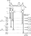
- the diagnostic device 10 has, as shown in FIG. 5, an acquisition unit 101 that acquires a learning signal and an input signal, and a first reference vector and a second reference vector that indicate a waveform that the input signal should have in a normal state.
- a learning unit 102 that learns from a learning signal, a storage unit 111 that stores a first reference vector learned by the learning unit 102, a storage unit 121 that stores a second reference vector learned by the learning unit 102, and an input signal
- a first calculation unit 110 for calculating a first index value indicating a distance between the input vector and the first reference vector
- a second calculation for calculating a second index value indicating an angle between the input vector and the second reference vector.
- Unit 120 a third calculation unit 130 that calculates an output value obtained by integrating the first index value and the second index value, and a diagnosis unit 140 that diagnoses the presence or absence of an abnormality from the output value.
- a thick arrow indicates a data flow when learning a reference vector from a learning signal
- a thin arrow indicates a data flow when calculating an output value from an input signal after completion of learning. ing.
- the acquisition unit 101 is mainly realized by the processor 11 and the communication unit 16.
- the acquisition unit 101 acquires a learning signal for learning a reference vector and an input signal to be monitored for the presence or absence of abnormality.
- the acquisition unit 101 acquires a learning signal provided by the user via the network 20.
- the learning signal is a signal that is long to some extent in order to sufficiently learn the reference vector, and includes all the waveforms of signals that should be input in a normal state.
- the acquisition unit 101 receives the input signal generated by the signal source 211 by repeatedly receiving data from the device 21 via the network 20.
- the acquisition unit 101 functions as an acquisition unit of claims.
- the learning unit 102 is mainly realized by the processor 11.
- the learning unit 102 learns the first reference vector for calculating the first index value and the second reference vector for calculating the second index value from the learning signal acquired by the acquisition unit 101.
- the learning unit 102 also includes a weight calculation unit 1021 that calculates the weights of the first reference vector and the second reference vector according to the learning result.
- the weight calculated by the weight calculation unit 1021 is provided to the third calculation unit 130.
- the learning unit 102 functions as a learning unit in claims.
- the learning signal is shown at the top of FIG.
- This learning signal has, as a waveform that the input signal should have in a normal state, a waveform 301 that sharply rises and then falls gently, a trapezoidal waveform 302, and a waveform 303 that rises gently and then falls sharply. Yes.
- the learning unit 102 divides the learning signal into a learning partial signal for learning a reference vector and a trial signal for calculating a weight.
- the vector extracted from the learning signal is used in the same manner as the extraction of the input vector from the input signal.
- the learning signal is a time-series signal of learning values that are sampling values, and the partial signal cut out from the learning signal is a sequence along the time of the learning value and is expressed as a vector.
- a vector corresponding to the partial signal cut out from the learning signal is referred to as a learning vector.
- the learning unit 3 extracts a learning value series from the learning partial signal, thereby learning vectors 311 having the learning values of this series as elements. Is generated. Then, the learning unit 102 learns one or more first reference vectors representing the learning vector 311 by clustering the plurality of learning vectors 311 according to the distance between the learning vectors 311. The learning unit 102 learns one or a plurality of second reference vectors representing the learning vector 311 by clustering according to the angle between the learning vectors 311.
- the distance between vectors is the distance between one vector and another vector, and is, for example, the Euclidean distance corresponding to the square root of the sum of square errors of each element of the vector.
- the present invention is not limited to this, and the distance between vectors may be a Manhattan distance, a distance defined by DTW (Dynamic Time Warping), or another distance. .
- the angle between vectors is an angle between one vector and another vector, and is a quantity whose unit is deg or rad.
- This angle is, for example, arccos (x) where x is a value obtained by dividing the inner product of one vector and another vector by the size of the one vector and the size of the other vector. Obtainable.
- Clustering according to the distance between the learning vectors 311 means that the scale for clustering the plurality of learning vectors 311 is a distance, and clustering according to the angle between the learning vectors 311 clusters the learning vectors 311. It means that the measure for it is an angle.
- Vector clustering is to combine a plurality of vectors into similar clusters according to a certain scale. Normally, a plurality of vectors are assigned to any one of the clusters. Any clustering method may be used, and for example, a k-means method or a mixed Gaussian model (GMM) may be employed. Different methods may be employed for clustering according to distance and clustering according to angle. Furthermore, the number of clusters may be defined in advance, or an appropriate number of clusters may be determined using a scale represented by AIC (Akaike Information Criteria).
- the first reference vector and the second reference vector may be a cluster center vector, or may be any learning vector 311 representing each cluster.
- a vector corresponding to each of a plurality of clusters formed by clustering according to the distance is learned as the first reference vector. That is, a plurality of vectors are learned as the first reference vector.
- a vector corresponding to each of the plurality of clusters corresponding to the angle is learned as the second reference vector. That is, a plurality of vectors are learned as the second reference vector.
- the distance from the first reference vector corresponding to the one cluster for the one vector is the other The distance is smaller than the distance from the first reference vector corresponding to any cluster.
- the angle between the one vector and the second reference vector corresponding to the one cluster is the other It becomes smaller than the distance from the second reference vector corresponding to any of the clusters.
- a single cluster may be formed as a result of clustering.
- the waveform to be input in the normal state is fixed to one pattern and this pattern appears in a period equal to the shift width of the window 310 shown in FIG. 311 may be clustered into one cluster.
- the weight calculation unit 1021 of the learning unit 102 determines the first reference for the trial signal in FIG. 6 according to the result of calculating the similarity using the first reference vector by the method shown in FIG. 4. Calculate the weight of the vector. Further, the weight calculation unit 1021 calculates the weight of the second reference vector according to the result of calculating the similarity using the second reference vector by the method shown in FIG. 4 for the trial signal.
- the similarity calculated using the second reference vector is a value in the range from zero to 1 according to the angle between the vectors. If the angle between the vectors is zero, the similarity is 1.
- the cosine cos ⁇ is calculated by the following equation (1).
- a ⁇ B in the above formulas (1) and (2) means an inner product of vectors
- “a1 ⁇ b1” means multiplication of components.
- the degree of similarity with the second reference vector may be calculated by another method according to the angle between the vectors.
- FIG. 7 shows an outline of weight calculation by the weight calculation unit 1021.
- the weight calculation unit 1021 slides the window 314 to cut out a series of trial values from the trial signal, thereby generating a plurality of trial vectors 315 having the trial values of this series as elements.
- the weight calculation unit 1021 selects the nearest vector from the first reference vector, and selects the nearest vector from the second reference vector.
- the weight calculation unit 1021 selects the first reference vector having the highest similarity to the trial vector 315 from the plurality of first reference vectors, and selects the first reference vector from the plurality of second reference vectors.
- the second reference vector having the highest degree of similarity with the trial vector 315 is selected.
- FIG. 7 shows an example of the similarity calculated for each reference vector. For example, when the similarity with each of the plurality of first reference vectors is calculated for one trial vector 315a among the trial vectors 315 shown in the upper part of FIG. 9 is the highest value. Further, when the similarity between each trial vector 315a and each of the plurality of second reference vectors is calculated, 0.9, which is the similarity with the second reference vector 317, is the highest value. In FIG. 7, for other trial vectors 315, numerical values indicating the similarity to the nearest vector among the first reference vectors are shown surrounded by squares, and the nearest vector of the second reference vectors and A numerical value indicating the degree of similarity is enclosed with a square.
- the weight calculation unit 1021 calculates the weight for each of the first reference vectors so that the weight increases as the average value of the calculated similarities increases. Further, the weight calculation unit 1021 calculates the weight for each second reference vector so that the weight becomes larger as the average value of the calculated similarities is larger. In other words, as the reference vector matches the waveform of the trial signal, the reference vector is given a higher weight. For example, the weight calculation unit 1021 directly adopts the average value of similarity as a weight. In the lower part of FIG. 7, for each reference vector, the average value of the numerical values appearing in the horizontal direction is calculated as a weight corresponding to the reference vector.
- the learning unit 102 stores the learned first reference vector in the storage unit 111 and stores the learned second reference vector in the storage unit 121.
- the storage units 111 and 121 are mainly realized by the auxiliary storage unit 13.
- the first calculation unit 110 is mainly realized by the processor 11.
- the first calculation unit 110 treats a series of input values acquired as an input signal by the acquisition unit 101 as an input vector having each input value of the series as an element.
- the dimension of this input vector is equal to the number of input values constituting the sequence acquired by the acquisition unit 101.
- the 1st calculation part 110 calculates a similarity degree by the method shown by FIG. Specifically, the first calculator 110 compares the input vector with each of the plurality of first reference vectors to calculate the similarity, and outputs the highest similarity as the first index value. More specifically, the first calculation unit 110 outputs a first index value indicating the distance between the input vector and the nearest first reference vector.
- the second calculation unit 120 is mainly realized by the processor 11. Similar to the first calculation unit 110, the second calculation unit 120 compares the input vector with the second reference vector to calculate the similarity by the method shown in FIGS. Output as an index value. Specifically, the second calculation unit 120 outputs a second index value indicating the angle between the input vector and the nearest second reference vector.
- the third calculation unit 130 is mainly realized by the processor 11.
- the third calculator 130 calculates an output value as a weighted sum of the first index value calculated by the first calculator 110 and the second index value calculated by the second calculator 120. Specifically, the third calculation unit 130 calculates the output value A3 by the calculation represented by the following equation (3).
- A1 is the first index value and A2 is the second index value.
- w1 is a weighting coefficient of the first index value, and is the weight of the nearest first reference vector selected by the first calculation unit 110 when calculating the first index value.
- w2 is a weighting coefficient of the second index value, and is the weight of the nearest second reference vector selected by the second calculation unit 120 when calculating the second index value.
- the third calculation unit 130 acquires these weights from the learning unit 102 in advance and holds them. Normally, the magnitudes of w1 and w2 are adjusted so that the sum thereof is 1.0, and the output value becomes a value within a range from zero to one.
- the diagnosis unit 140 is mainly realized by the processor 11, the output unit 15, or the communication unit 16.
- the diagnosis unit 140 diagnoses the presence / absence of an abnormality based on the output value calculated by the third calculation unit 130. For example, the diagnosis unit 140 determines whether there is an abnormality by determining whether the output value exceeds a threshold value. This threshold is 0.8, for example, and may be defined in advance or may be changed by the user.
- the output of the diagnosis result information by the diagnosis unit 140 may be presented to the user by screen display, may be output to a signal processing circuit included in the diagnosis device 10, or may be data via the network 20. May be transmitted.
- the diagnosis unit 140 functions as a diagnosis unit in the claims.
- the diagnostic process shown in FIG. 8 starts when the diagnostic apparatus 10 is turned on.
- the diagnosis device 10 executes a learning process (step S1) and executes a diagnosis execution process (step S2).
- step S1 the learning process and the diagnosis execution process will be described in order.
- FIG. 9 shows a learning process procedure.
- the learning process is a process of learning the reference vector from the learning signal, and is mainly executed by the learning unit 102.
- the acquisition unit 101 acquires a learning signal (step S11). Specifically, the acquisition unit 101 acquires data indicating a learning signal and extracts the learning signal from the data.
- the learning unit 102 divides the learning signal acquired in step S11 into a learning partial signal and a trial signal (step S12). Specifically, the learning unit 102 equally divides the learning signal into the former stage and the latter stage.
- the division method is arbitrary and may be divided by other methods.
- the learning unit 102 generates a plurality of learning vectors by cutting out a sequence of learning values from the learning partial signal (step S13). Then, the learning unit 102 learns the first reference vector by clustering the learning vectors according to the distance between the vectors (step S14), and clusters the learning vectors according to the angle between the vectors to obtain the second reference vector. A vector is learned (step S15).
- the learning unit 102 calculates a weight for the trial signal according to the result of calculating the similarity (step S16). Specifically, the weight calculation unit 1021 calculates the weights of the first reference vector and the second reference vector according to the result of comparing the trial signal with the first reference vector and the second reference vector. Thereafter, the learning process ends, and the process performed by the diagnostic device 10 returns to the diagnostic process shown in FIG.
- the diagnosis execution process is a process for diagnosing whether there is an abnormality by calculating an output value from an input signal.
- the acquisition unit 101 acquires a series of input values as an input signal (step S21).
- This step S21 corresponds to an acquisition step of claims.
- the series acquired here corresponds to partial signals delimited by the window 26 shown in FIG.
- the series of input values is treated as an input vector whose elements are input values.
- the first calculation process is a process in which the first calculation unit 110 calculates a first index value from the input vector acquired in step S21.
- the first calculation unit 110 extracts a first nearest neighbor vector similar to the input vector from the first reference vector (step S221). Then, the first calculation unit 110 outputs the similarity between the input vector and the first nearest neighbor vector as a first index value (step S222). Thereafter, the first calculation process ends, and the process performed by the diagnostic device 10 returns to the diagnosis execution process of FIG.
- the second calculation process is a process in which the second calculation unit 120 calculates the second index value from the input vector acquired in step S21.
- the second calculation unit 120 extracts a second nearest neighbor vector similar to the input vector from the second reference vector (step S231). Then, the second calculation unit 120 outputs the similarity between the input vector and the second nearest neighbor vector as a second index value (step S232). Thereafter, the second calculation process ends, and the process performed by the diagnostic device 10 returns to the diagnosis execution process of FIG.
- the third calculation unit 130 executes the third calculation process (step S24). Specifically, the third calculation unit 130 calculates an output value as a weighted sum of the first index value calculated in step S22 and the second index value calculated in step S23.
- step S25 corresponds to the diagnostic step of the claims.
- the diagnostic apparatus 10 repeats the processes after step S21.
- the diagnostic apparatus 10 the first index value indicating the distance between the input vector and the first reference vector, the second index value indicating the angle between the input vector and the second reference vector, The presence or absence of abnormality is diagnosed. For this reason, it is expected that accurate diagnosis based on the angle between the vectors is expected even when the diagnosis is made erroneously only by the distance between the vectors. Therefore, it is possible to improve the diagnostic accuracy of the presence or absence of abnormality.
- FIG. 13 shows an example in which the input signal has a waveform that rises steeply and falls slowly, and each input value is twice the value of the learning signal.
- the first reference vector R1 having the shortest Euclidean distance among the first reference vectors R1, R2, and R3 indicated by black circles at the bottom of FIG. 13 is the first nearest neighbor. Selected as vector R1.
- the distance between the vectors is taken as a scale
- the vector closest to the vector A1 among the first reference vectors R1, R2, and R3 is R1
- the waveform thereof is shown in the upper part of FIG. It is a trapezoid.
- the scale of the waveform of the input vector is simply changed from the time of learning, and if it is compared with the trapezoidal waveform, the presence or absence of abnormality cannot be correctly diagnosed.
- the diagnostic apparatus 10 calculates an output value by integrating the first index value and the second index value. For this reason, it is expected that abnormality diagnosis by the diagnostic device 10 is performed more accurately than when the diagnosis is performed based only on the distance between vectors. Specifically, even when the scale of the value of the input signal can be changed in the normal state, since the second index value based on the angle between the vectors is taken into account to diagnose the presence / absence of an abnormality, the occurrence of a false diagnosis It is expected to reduce the rate.
- diagnosis unit 140 diagnoses the presence or absence of an abnormality from the output value calculated by the third calculation unit as a weighted sum of the first index value and the second index value. For this reason, it is possible to easily realize sequential execution of diagnoses with a relatively small calculation load necessary for diagnosis.
- the learning unit 102 learned the reference vector from the learning signal, and the weight of the reference vector was calculated according to the learning result. For this reason, the first index value and the second index value can be weighted according to learning to diagnose the presence or absence of abnormality.
- the learning signal is a signal indicating a waveform to be input at the normal time, and the normal waveform indicated by the learning signal varies to some extent. It is considered that a more accurate diagnosis can be made by assigning such a weighting factor to the reference vector.
- the learning unit 102 learned the reference vector by clustering the learning vectors.
- the amount of calculation becomes excessively large.
- the learning unit 102 can efficiently learn the reference vector used for diagnosis by performing clustering.
- the learning unit 102 divides the learning signal into a learning partial signal and a trial signal, learns a reference vector from the learning partial signal, and calculates a weight of the reference vector from the trial signal.
- the trial signal can be said to be a signal for trying to calculate the similarity using the learned reference vector. It is expected that an effective weight is calculated in the subsequent diagnosis execution process by obtaining the weight with a signal different from the signal for learning the reference vector.
- the weight calculation unit 1021 calculates, as a weight, the average value of the similarities calculated when the reference vector is selected as the nearest vector of the trial vector, but is not limited thereto.
- the weight calculation unit 1021 may calculate the weight according to the change in similarity calculated for the trial vector. Specifically, the weight calculation unit 1021 may calculate a larger weight as the variation in similarity is smaller. As such a weight, for example, a weight corresponding to a statistical value represented by a standard deviation of similarity can be considered.
- Embodiment 2 the second embodiment will be described focusing on the differences from the first embodiment.
- the description is abbreviate
- the weights assigned to the first reference vector and the second reference vector are calculated from the learning signal, but other forms are also conceivable.
- the weight is determined based on the magnitude of the index value will be described.
- Diagnostic device 10 is configured by omitting learning unit 102 as shown in FIG.
- the storage units 111 and 121 the first reference vector and the second reference vector are stored in advance by the user. Then, every time the first index value and the second index value are calculated, the third calculation unit 130 determines the weight to be multiplied by these index values and then calculates the output value.
- FIG. 15 shows the relationship between the difference between the first index value and the second index value and the weight. Specifically, for the difference obtained by subtracting the second index value from the first index value, the weight of the first index value is indicated by line L1, and the weight of the second index value is indicated by line L2. Yes. These lines L1 and L2 indicate that the larger weight coefficient of the first index value and the second index value is increased, and the weight coefficient is made equal when the first index value and the second index value are equal. Show.
- the third calculation unit 130 calculates an output value that emphasizes the larger one of the first index value and the second index value. Therefore, when the distance or angle between the input vector and the reference vector is close, the output value indicating the degree of similarity of the waveforms becomes large. This output value can be used for more accurate diagnosis of abnormality.
- the determination of the weight by the third calculation unit 130 is not limited to the example shown in FIG.
- the weight of one of the first index value and the second index value may be set to 1, and the other weight may be set to zero.
- the larger one of the first index value and the second index value is substantially adopted as the output value.
- the weight may be determined for the ratio between the first index value and the second index value.
- the reciprocal of the quotient obtained by dividing the first index value by the second index value is used as the weight of the first index value.
- Embodiment 3 the third embodiment will be described focusing on the differences from the first embodiment.
- the description is abbreviate
- the weight is determined using the trial signal divided from the learning signal.
- the weight may be determined without dividing the learning signal.
- an example will be described in which the weight is determined according to the result of learning the reference vector without dividing the learning signal.
- FIG. 18 schematically shows an example in which the first reference vector is determined from the learning signal.
- learning vectors o1 to o7 extracted from such learning signals being clustered using the distance as a scale, clusters D1 to D3 are formed.
- first reference vectors s1 to s3 representing each of the clusters D1 to D3 are generated.
- FIG. 19 schematically shows an example in which the second reference vector is determined from the learning signal similar to FIG.
- clusters E1 and E2 are formed.
- second reference vectors v1 and v2 representing the clusters E1 and E2 are generated.
- FIG. 20 compares the number of learning vectors belonging to the cluster corresponding to each first reference vector and the number of learning vectors belonging to the cluster corresponding to each second reference vector. For example, the number of learning vectors based on the first reference vector s1 is two, and the number of learning vectors based on the second reference vector v2 is five.
- the learning unit 102 determines a weighting coefficient to be given to the reference vector according to the number of learning vectors belonging to the cluster corresponding to each reference vector. Specifically, the weighting factor is increased as the number of learning vectors increases. More specifically, a weighting factor of 1.0 is assigned to the reference vector that maximizes the number of learning vectors, and a weighting factor that is proportional to the number of learning vectors is assigned to the other reference vectors.
- the method for determining the weighting coefficient is not limited to this and is arbitrary.
- the third calculation unit 130 weights and adds the first index value and the second index value, and the weighting factor assigned to the first reference vector selected to calculate the first index value; And a weighting factor assigned to the second reference vector selected to calculate the second index value.
- the third calculation unit 130 may adjust the size of the weighting factor so that the sum becomes 1.0.
- the diagnostic apparatus 10 determines the weight according to the number of learning vectors clustered into clusters corresponding to each reference vector. It is considered that the reference vectors corresponding to many learning vectors accurately represent the waveform to be input at the normal time. By giving a large weight to such an accurate reference vector, it is considered that the output value calculated by the third calculation unit 130 can be used for accurate abnormality diagnosis.
- the weight coefficient may be obtained by multiplying the base value common to all clusters of the first reference vector by the cluster value of each cluster.
- a weight coefficient may be obtained by multiplying the base value common to all clusters of the second reference vector by the cluster value of each cluster.
- the learning signal shown in FIG. 21 includes an arc-shaped waveform, a triangular waveform, and a rectangular waveform, and has a plurality of waveforms with different scales for each waveform.
- An example of learning the first reference vector and the second reference vector from such a learning signal is schematically shown in FIG.
- FIG. 22 six first reference vectors and three second reference vectors are learned from the eight learning vectors.
- the base value is calculated as 1.33 for all the first reference vectors. Specifically, a value of 1.33 is calculated as a base value by dividing 8 which is the number of learning vectors by 6 which is the number of first reference vectors.
- the base value is calculated to be 2.66 for all the second reference vectors. Specifically, a value of 2.66 is calculated as a base value by dividing 8 which is the number of learning vectors by 3 which is the number of second reference vectors.
- a new weighting factor may be obtained by multiplying this base value by, for example, a value equal to the weighting factor shown in FIG.
- a larger base value is assigned to the smaller one of the first reference vector and the second reference vector. It can be said that the smaller the number of clusters, the more learning vectors belong to each cluster. Since a cluster to which many learning vectors belong can be said to appropriately represent a waveform to be inputted in a normal state, as a result, a larger weight is given to the one that appropriately represents the waveform among the first reference vector and the second reference vector. Will be granted.
- the learning signal shown in FIG. 23 has the same waveform as that in FIG. 21, but the scale is fixed for each waveform.
- An example of learning the first reference vector and the second reference vector from such a learning signal is schematically shown in FIG. As shown in FIG. 24, three first reference vectors and three second reference vectors are learned from the eight learning vectors. In this example, the base value is calculated as 2.66 for both the first reference vector and the second reference vector. For this reason, the 3rd calculation part 130 will calculate an output value by giving equal weight to the 1st index value and the 2nd index value, and carrying out weighting addition.
- the diagnostic apparatus 10 may determine the weight according to the tendency of the number of learning vectors clustered into clusters corresponding to each reference vector. Regarding the weights determined in this way, it is considered that the output value calculated by the third calculation unit 130 can be used for accurate diagnosis of abnormality.
- diagnosis system 100 is a part of the production system
- present invention is not limited to this.
- the diagnosis system 100 may be a part of a processing system represented by a processing system or an inspection system, or may be an independent system without constituting another system.
- the acquisition unit 101 of the diagnostic apparatus 10 acquires an input signal via the network 20
- the present invention is not limited to this.
- the acquisition unit 101 may read an input signal from data stored in the auxiliary storage unit 13 by the user.
- the diagnostic apparatus 10 may acquire a plurality of input signals and calculate an output value for each of the input signals, or may output a single output value by integrating the output values calculated for each of the input signals. Also good.
- the number of index values integrated to calculate the output value is two. It is not limited to 3 or more.
- an output value may be calculated by integrating a third index value different from both the first index value and the second index value with the first index value and the second index value.
- the first index value, the second index value, and the output value are values that become smaller as the degree of abnormality increases.
- the present invention is not limited to this, and the degree of abnormality is strong. The value which becomes so large may be sufficient.
- the function of the diagnostic apparatus 10 can be realized by dedicated hardware or by a normal computer system.
- the program P1 executed by the processor 11 is stored in a computer-readable non-transitory recording medium and distributed, and the program P1 is installed in the computer to constitute an apparatus that executes the above-described processing. be able to.
- a recording medium for example, a flexible disk, a CD-ROM (Compact Disc-Read-Only Memory), a DVD (Digital Versatile Disc), and an MO (Magneto-Optical Disc) can be considered.
- the program P1 may be stored in a disk device included in a server device on a communication network represented by the Internet, and may be downloaded onto a computer, for example, superimposed on a carrier wave.
- the above-described processing can also be achieved by starting and executing the program P1 while transferring it via the communication network.
- processing can also be achieved by executing all or part of the program P1 on the server device, and executing the program while the computer transmits / receives information related to the processing via the communication network.
- the means for realizing the function of the diagnostic apparatus 10 is not limited to software, and part or all of the means may be realized by dedicated hardware including a circuit.
- the present invention is suitable for diagnosing an abnormality indicated by a signal.
- diagnostic system 10 diagnostic device, 11 processor, 12 main storage unit, 13 auxiliary storage unit, 14 input unit, 15 output unit, 16 communication unit, 17 internal bus, 101 acquisition unit, 102 learning unit, 110 first calculation unit , 111 storage unit, 120 second calculation unit, 121 storage unit, 130 third calculation unit, 140 diagnostic unit, 1021 weight calculation unit, 20 network, 21 device, 211 signal source, 23, 24 waveform, 26 window, 27 memory 301-303 waveform, 310, 314 window, 311 learning vector, 315, 315a trial vector, 316 first reference vector, 317 second reference vector, L1, L2 line, P1 program.
Landscapes
- Engineering & Computer Science (AREA)
- Data Mining & Analysis (AREA)
- Theoretical Computer Science (AREA)
- Physics & Mathematics (AREA)
- Evolutionary Computation (AREA)
- Artificial Intelligence (AREA)
- General Physics & Mathematics (AREA)
- Bioinformatics & Computational Biology (AREA)
- Computer Vision & Pattern Recognition (AREA)
- Evolutionary Biology (AREA)
- Bioinformatics & Cheminformatics (AREA)
- General Engineering & Computer Science (AREA)
- Life Sciences & Earth Sciences (AREA)
- Mathematical Physics (AREA)
- Automation & Control Theory (AREA)
- Probability & Statistics with Applications (AREA)
- Testing And Monitoring For Control Systems (AREA)
Abstract
診断装置(10)は、取得部(101)と診断部(140)とを備える。取得部(101)は、異常の有無の診断対象となる入力信号として入力値の系列を取得する。診断部(140)は、取得部(101)によって取得された系列の入力値を要素とする入力ベクトルと予め定められた第1基準ベクトルとの距離を示す第1指標値と、入力ベクトルと予め定められた第2基準ベクトルとの角度を示す第2指標値と、から異常の有無を診断する。
Description
本発明は、診断装置、診断方法及びプログラムに関する。
工場における生産システム及び制御システムのように、センサによるセンシング結果を示す時系列データを利用する種々の処理システムが知られている。この種の処理システムでは、時系列データから異常の有無を診断することが広く行われている。
具体的には、監視対象の信号波形が正常時に入力されるべき波形と類似するか否かを判別することで異常の診断をする技術がある(例えば、特許文献1を参照)。特許文献1には、現在の時系列データである入力ベクトルと、データベースに蓄積されている過去の時系列データである入力ベクトルとの間の距離に基づいて異常測度を算出する技術について記載されている。
しかしながら、信号波形が類似するか否かを判別するための尺度としては、特許文献1のようなベクトル間の距離が不適当となるケースもある。例えば、入力ベクトルの要素の比率を維持したまま値の大きさが変動し得るケースにおいて、特許文献1の技術では、入力ベクトルの大きさが変化したときに誤って異常と判断されるおそれがある。このため、異常の有無の診断精度を向上させる余地があった。
本発明は、上記の事情に鑑みてなされたものであり、異常の有無の診断精度を向上させることを目的とする。
上記目的を達成するため、本発明の診断装置は、異常の有無の診断対象となる入力信号として入力値の系列を取得する取得手段と、取得手段によって取得された系列の入力値を要素とする入力ベクトルと予め定められた第1基準ベクトルとの距離を示す第1指標値と、入力ベクトルと予め定められた第2基準ベクトルとの角度を示す第2指標値と、から異常の有無を診断する診断手段と、を備える。
本発明によれば、入力ベクトルと第1基準ベクトルとの距離を示す第1指標値と、入力ベクトルと第2基準ベクトルとの角度を示す第2指標値と、から異常の有無が診断される。このため、ベクトル間の距離だけでは誤って診断をされるような場合においても、ベクトル間の角度に基づいて正確な診断をすることが期待される。したがって、異常の有無の診断精度を向上させることができる。
以下、本発明の実施の形態に係る診断システム100について、図面を参照しつつ詳細に説明する。
実施の形態1.
本実施の形態に係る診断システム100は、工場に形成される生産システムの一部に相当する。診断システム100は、生産システムからデータを収集して、収集したデータから、当該生産システムにおける異常の有無を診断する。異常は、例えば、生産ラインに流れるワークの仕様が規格外であること、生産ラインを構成する装置の不具合、及びこの装置の稼働中に生じたエラーを含む。異常は、生産システムの運営者が想定するものとして予め定められる正常な状態とは異なる状態であって、通常は、生産システムによる製品の生産を停止させ、又は歩留まりを低下させる。そして、診断システム100は、診断の結果を示す情報をユーザに提供する。診断システム100は、図1に示されるように、異常の有無を診断する診断装置10と、診断装置10に信号を送信する複数の機器21と、を有している。なお、図1では、1つの機器21が代表して示されている。
本実施の形態に係る診断システム100は、工場に形成される生産システムの一部に相当する。診断システム100は、生産システムからデータを収集して、収集したデータから、当該生産システムにおける異常の有無を診断する。異常は、例えば、生産ラインに流れるワークの仕様が規格外であること、生産ラインを構成する装置の不具合、及びこの装置の稼働中に生じたエラーを含む。異常は、生産システムの運営者が想定するものとして予め定められる正常な状態とは異なる状態であって、通常は、生産システムによる製品の生産を停止させ、又は歩留まりを低下させる。そして、診断システム100は、診断の結果を示す情報をユーザに提供する。診断システム100は、図1に示されるように、異常の有無を診断する診断装置10と、診断装置10に信号を送信する複数の機器21と、を有している。なお、図1では、1つの機器21が代表して示されている。
診断装置10と機器21とは、ネットワーク20を介して互いに通信可能となるように接続される。ネットワーク20は、産業用のFAネットワークである。ただし、ネットワーク20は、これに限定されず、広域通信のための通信ネットワークであってもよいし、専用線であってもよい。
機器21は、例えば、センサ装置、アクチュエータ又はロボットである。機器21は、信号源211としてのセンサを有する。機器21は、このセンサによるセンシング結果を、ネットワーク20を介して繰り返し診断装置10に通知することにより、センシング結果の推移を示すデジタル信号を診断装置10に送信する。センサは、例えば、圧力センサ、照度センサ、超音波センサ又はその他のセンサである。機器21から送信される信号は、スカラー値の時系列信号であって、そのサンプリング周期は、例えば10ms、100ms、又は1secである。
ただし、機器21から送信される信号は、スカラー値に限らず、ベクトル値の信号であってもよい。また、機器21は、センサのサンプリング周期とは異なる周期で診断装置10にデータを送信してもよい。例えば、機器21は、センサによるサンプリング値がバッファにある程度蓄積されたときに、蓄積されたサンプリング値を含むデータを診断装置10に送信してもよい。信号源211は、センサの他、例えば、生産システムにおける機器21の動作を同期させるための同期信号を生成する発振器、又は、遠隔の対向機器と通信する受信機若しくはアンテナであってもよい。
診断装置10は、工場に配置されるIPC(Industrial Personal Computer)である。診断装置10は、そのハードウェア構成として、図2に示されるように、プロセッサ11と、主記憶部12と、補助記憶部13と、入力部14と、出力部15と、通信部16と、を有する。主記憶部12、補助記憶部13、入力部14、出力部15及び通信部16はいずれも、内部バス17を介してプロセッサ11に接続される。
プロセッサ11は、CPU(Central Processing Unit)を含む。プロセッサ11は、補助記憶部13に記憶されるプログラムP1を実行することにより、診断装置10の種々の機能を実現して、後述の処理を実行する。
主記憶部12は、RAM(Random Access Memory)を含む。主記憶部12には、補助記憶部13からプログラムP1がロードされる。そして、主記憶部12は、プロセッサ11の作業領域として用いられる。
補助記憶部13は、EEPROM(Electrically Erasable Programmable Read-Only Memory)及びHDD(Hard Disk Drive)に代表される不揮発性メモリを含む。補助記憶部13は、プログラムP1の他に、プロセッサ11の処理に用いられる種々のデータを記憶する。補助記憶部13は、プロセッサ11の指示に従って、プロセッサ11によって利用されるデータをプロセッサ11に供給し、プロセッサ11から供給されたデータを記憶する。なお、図2では、1つのプログラムP1が代表的に示されているが、補助記憶部13は、複数のプログラムを記憶してもよいし、主記憶部12には、複数のプログラムがロードされてもよい。
入力部14は、入力キー及びポインティングデバイスに代表される入力デバイスを含む。入力部14は、診断装置10のユーザによって入力された情報を取得して、取得した情報をプロセッサ11に通知する。
出力部15は、LCD(Liquid Crystal Display)及びスピーカに代表される出力デバイスを含む。出力部15は、プロセッサ11の指示に従って、種々の情報をユーザに提示する。
通信部16は、外部の装置と通信するためのネットワークインタフェース回路を含む。通信部16は、外部から信号を受信して、この信号により示されるデータをプロセッサ11へ出力する。また、通信部16は、プロセッサ11から出力されたデータを示す信号を外部の装置へ送信する。
図2に示されるハードウェア構成が協働することにより、診断装置10は、異常の有無を診断して、診断結果を示す情報を出力する。詳細には、診断装置10は、後述の手法で信号を分析した結果として異常の有無を診断する。
ここで、診断装置10による信号分析の基本的な手法について、図3,4を用いて説明する。図3には、異常の診断の概要が示されている。図3上部には、診断装置10に入力される入力信号が示されている。この入力信号は、正常時には、複数の波形パターンのいずれか1つと類似する波形を有する。このため、入力信号の波形がいずれの波形パターンからも乖離する形状である場合には、異常であると判定される。
図3における入力信号の最初の波形23は、複数の波形パターンA,B,Cそれぞれと比較された結果、波形パターンAと比較したときに最高の類似度である0.99を示す。この最高類似度が閾値を超えているため、波形23に関しては正常と判断される。類似度は、波形同士が類似する度合いを示すゼロから1までの範囲の値であって、波形が一致する場合には類似度が1になる。類似度の算出手法については、後述する。また、閾値は、例えば0.8であって、予め規定されてもよいし、ユーザによって設定されてもよい。
引き続き、入力信号の波形が波形パターンA,C,C,C,B,Aに最も類似すると順に判定され、その類似度は0.91,0.92,0.89,0.85,0.98,0.55と順に算出される。最後の波形24に関して、複数の波形パターンA,B,Cのうち最も類似するパターンは波形パターンAであるが、その類似度は閾値より低い0.55である。このため、最後の波形24については異常であると判定される。
図4には、波形を比較するための入力信号の切り出しについて示されている。図4に示されるように、診断装置10は、予め規定された幅のウィンドウ26を一定のシフト幅でスライドさせる。ウィンドウ26は、入力信号の一部を切り出すための窓であって、例えば、一部の区間の値を1として他の値をゼロとして規定される矩形の窓関数のうちの値が1である区間に相当し、この窓関数を入力信号に乗じることで入力信号の一部が切り出される。診断装置10は、ウィンドウ26をスライドさせる度に、ウィンドウ26に相当する区間の部分信号を入力信号から切り出す。そして、メモリ27に予め記憶される波形パターンから、部分信号の最近傍のパターンを抽出して、部分信号と最近傍パターンとを比較した結果としての類似度を得る。ここで、最近傍のパターンは、類似度が最高になる波形パターンを意味する。
波形パターンは、正常時に入力信号が有するべき波形であって、予めメモリ27に格納される。詳細には、図4に示されるように、入力信号から一定のシフト幅で切り出された部分信号について異常の有無を判定するために、診断装置10は、正常時に入力されるべき波形が時間方向にシフトしたパターンを予め波形パターンとして記憶している。
なお、入力信号から切り出される部分信号は、デジタル信号であり、サンプリング値の時間に沿った系列であるため、ベクトルとしても表現される。系列は、値が一続きになったまとまりを意味する。また、波形パターンについても入力信号と同様にベクトルとして表現されれば、ベクトルの演算により波形を比較することができるため都合がよい。
診断装置10は、上述のような波形の比較を2通りの手法で行い、それぞれの手法の結果を統合することで異常の有無を診断する。これら2通りの手法のうち、第1の手法は、入力信号と波形パターンとの距離に着目する手法であって、第2の手法は、入力信号と波形パターンとの角度に着目する手法である。詳細には、第1の手法は、入力信号から切り出された部分信号に相当するベクトルである入力ベクトルと、第1の手法で用いる波形パターンに相当するベクトルである第1基準ベクトルと、の距離により、これらのベクトルが類似する度合いを示す第1指標値を得る手法である。また、第2の手法は、入力信号から切り出された部分信号に相当する入力ベクトルと、第2の手法で用いる波形パターンに相当するベクトルである第2基準ベクトルと、の角度により、これらのベクトルが類似する度合いを示す第2指標値を得る手法である。
第1基準ベクトル及び第2基準ベクトルは、正常時に入力ベクトルが有するべき波形を示すベクトルであって、2通りの手法それぞれに適した第1基準ベクトル及び第2基準ベクトルを異常の診断に先立って予め準備する必要がある。診断装置10は、これらの第1基準ベクトル及び第2基準ベクトルを学習する機能を有する。詳細には、診断装置10は、正常時に入力されるべき波形を示すものとしてユーザから提供される学習信号から、第1基準ベクトル及び第2基準ベクトルを学習する機能を有する。そして、学習の終了後に、診断装置10は、学習した第1基準ベクトル及び第2基準ベクトルを利用して、診断対象となる入力信号について異常の有無を診断する。以下では、第1基準ベクトル及び第2基準ベクトルを総称して単に基準ベクトルという。
また、第1指標値は、入力ベクトルにより示される波形と、第1基準ベクトルにより示される波形と、が類似する度合いを示す指標となる値であって、これらの波形の類似度に相当する。また、第2指標値は、入力ベクトルにより示される波形と、第2基準ベクトルにより示される波形と、が類似する度合いを示す指標となる値であって、これらの波形の類似度に相当する。第1指標値及び第2指標値の算出手法の詳細については、後述する。
診断装置10は、その機能として、図5に示されるように、学習信号及び入力信号を取得する取得部101と、正常時に入力信号が有するべき波形を示す第1基準ベクトル及び第2基準ベクトルを学習信号から学習する学習部102と、学習部102によって学習された第1基準ベクトルを記憶する記憶部111と、学習部102によって学習された第2基準ベクトルを記憶する記憶部121と、入力信号としての入力ベクトルと第1基準ベクトルとの距離を示す第1指標値を算出する第1算出部110と、入力ベクトルと第2基準ベクトルとの角度を示す第2指標値を算出する第2算出部120と、第1指標値と第2指標値とを統合した出力値を算出する第3算出部130と、出力値から異常の有無を診断する診断部140と、を有する。なお、図5中、太い矢印は、学習信号から基準ベクトルを学習する際のデータの流れを示し、細い矢印は、学習の終了後に、入力信号から出力値を算出する際のデータの流れを示している。
取得部101は、主としてプロセッサ11及び通信部16によって実現される。取得部101は、基準ベクトルを学習するための学習信号と、異常の有無の監視対象となる入力信号と、を取得する。詳細には、取得部101は、ユーザによってネットワーク20を介して提供される学習信号を取得する。学習信号は、基準ベクトルを十分に学習するためにある程度長い信号であって、正常時に入力されるべき信号の波形をすべて含むことが望ましい。また、取得部101は、機器21からネットワーク20を介してデータを繰り返し受信することにより、信号源211によって生成された入力信号を受信する。取得部101は、請求項の取得手段として機能する。
学習部102は、主としてプロセッサ11によって実現される。学習部102は、取得部101によって取得された学習信号から、第1指標値を算出するための第1基準ベクトル、及び第2指標値を算出するための第2基準ベクトルを学習する。また、学習部102は、学習の結果に応じて第1基準ベクトル及び第2基準ベクトルそれぞれの重みを算出する重み算出部1021を有する。重み算出部1021によって算出された重みは、第3算出部130に提供される。学習部102は、請求項の学習手段として機能する。
ここで、学習部102による基準ベクトルの学習の概要について、図6を用いて説明する。図6の最上段には、学習信号が示されている。この学習信号は、正常時に入力信号が有するべき波形として、急峻に立ち上がってから緩やかに下がる波形301と、台形状の波形302と、緩やかに立ち上がってから急峻に下がる波形303と、を有している。学習部102は、この学習信号を、基準ベクトルを学習するための学習部分信号と、重みを算出するための試行信号と、に分割する。
学習部102が基準ベクトルを学習するために、入力信号からの入力ベクトルの抽出と同様に、学習信号から抽出されたベクトルが用いられる。学習信号は、サンプリング値である学習値の時系列信号であり、学習信号から切り出される部分信号は、この学習値の時間に沿った系列であって、ベクトルとして表現される。以下では、学習信号から切り出された部分信号に相当するベクトルを学習ベクトルという。
詳細には、図6に示されるように、学習部102は、ウィンドウ310をスライドさせる度に、学習部分信号から学習値の系列を切り出すことにより、この系列の学習値を要素とする学習ベクトル311を生成する。そして、学習部102は、学習ベクトル311間の距離に応じて複数の学習ベクトル311をクラスタリングすることにより、学習ベクトル311を代表する一又は複数の第1基準ベクトルを学習する。また、学習部102は、学習ベクトル311間の角度に応じてクラスタリングすることにより学習ベクトル311を代表する一又は複数の第2基準ベクトルを学習する。
ここで、ベクトル間の距離は、一のベクトルと他のベクトルとの距離であって、例えば、ベクトルの各要素の自乗誤差の総和の平方根に相当するユークリッド距離である。ただし、これには限定されず、ベクトル間の距離は、マンハッタン距離であってもよいし、DTW(Dynamic Time Warping)により規定される距離であってもよいし、他の距離であってもよい。
また、ベクトル間の角度は、一のベクトルと他のベクトルとの角度であって、単位をdeg又はradとする量である。この角度は、例えば、一のベクトルと他のベクトルとの内積を、当該一のベクトルの大きさと当該他のベクトルの大きさとで除して得た値をxとしたときのarccos(x)として得ることができる。
学習ベクトル311間の距離に応じたクラスタリングは、複数の学習ベクトル311をクラスタリングするための尺度を距離とすることを意味し、学習ベクトル311間の角度に応じたクラスタリングは、学習ベクトル311をクラスタリングするための尺度を角度とすることを意味する。ベクトルのクラスタリングは、複数のベクトルを、ある尺度に従って類似するベクトルをクラスタにまとめることであって、通常は、複数のベクトルがそれぞれいずれかのクラスタに振り分けられる。クラスタリングの手法は任意であって、例えばk平均法又は混合ガウシアンモデル(GMM; Gaussian Mixture Model)を採用してもよい。また、距離に応じたクラスタリングと角度に応じたクラスタリングとで異なる手法を採用してもよい。さらに、クラスタ数は、予め規定されてもよいし、AIC(Akaike Information Criteria)に代表される尺度を用いて適当なクラスタ数を決定してもよい。
第1基準ベクトル及び第2基準ベクトルは、クラスタ中心のベクトルであってもよいし、各クラスタを代表するいずれかの学習ベクトル311であってもよい。通常は、距離に応じたクラスタリングにより形成された複数のクラスタそれぞれに対応するベクトルが第1基準ベクトルとして学習される。すなわち、複数のベクトルが第1基準ベクトルとして学習される。また、角度に応じた複数のクラスタそれぞれに対応するベクトルが第2基準ベクトルとして学習される。すなわち、複数のベクトルが第2基準ベクトルとして学習される。
例えば、距離に応じたクラスタリングの結果、一のベクトルが一のクラスタに属することとなった場合、当該一のベクトルについては、当該一のクラスタに対応する第1基準ベクトルとの距離が、他のいずれのクラスタに対応する第1基準ベクトルとの距離よりも小さくなる。同様に、角度に応じたクラスタリングの結果、一のベクトルが一のクラスタに属することとなった場合、当該一のベクトルについては、当該一のクラスタに対応する第2基準ベクトルとの角度が、他のいずれのクラスタに対応する第2基準ベクトルとの距離よりも小さくなる。
ただし、クラスタリングの結果、単一のクラスタのみが形成される場合も想定される。例えば、正常時に入力されるべき波形が1つのパターンに固定されており、このパターンが、図6に示されるウィンドウ310のシフト幅に等しい周期で現れるようなケースでは、実質的に同等の学習ベクトル311が、1つのクラスタにクラスタリングされ得る。
図5に戻り、学習部102の重み算出部1021は、図6中の試行信号について、図4に示される手法により第1基準ベクトルを用いて類似度を算出した結果に応じて、第1基準ベクトルの重みを算出する。また、重み算出部1021は、試行信号について、図4に示される手法により第2基準ベクトルを用いて類似度を算出した結果に応じて、第2基準ベクトルの重みを算出する。
第1基準ベクトルを用いて算出される類似度は、ベクトル間の距離をゼロから1の範囲内におさまるように正規化することで算出される。ベクトルが同一であれば、ベクトル間の距離はゼロとなり、類似度は1になる。例えば、ベクトル間の距離をDとして、類似度Eは、E=1/(1+D)として算出される。ただし、類似度Eを得るための算出式は、これに限定されず任意である。
また、第2基準ベクトルを用いて算出される類似度は、ベクトル間の角度に応じたゼロから1の範囲内の値である。ベクトル間の角度がゼロであれば、類似度は1となる。例えば、ベクトル間の角度をθとして、類似度Fは、F=(cosθ/2)+(1/2)として算出される。ここで、ベクトルAの成分を(a1,a2)とし、ベクトルBの成分を(b1,b2)とすると、余弦cosθは、次式(1)により算出される。
cosθ=(A・B)/|A||B|
=(a1・b1+a2・b2)/((a12+a22)1/2(b12+b22)1/2) ・・・(1)
=(a1・b1+a2・b2)/((a12+a22)1/2(b12+b22)1/2) ・・・(1)
ベクトルA,Bが3次元である場合には、ベクトルAの成分を(a1,a2,a3)とし、ベクトルBの成分を(b1,b2,b3)とすると、余弦cosθは、次式(2)により算出される。
cosθ=(A・B)/|A||B|
=(a1・b1+a2・b2+a3・b3)/((a12+a22+a32)1/2(b12+b22+b32)1/2) ・・・(2)
=(a1・b1+a2・b2+a3・b3)/((a12+a22+a32)1/2(b12+b22+b32)1/2) ・・・(2)
ただし、上記式(1),(2)中の「A・B」は、ベクトルの内積を意味し、「a1・b1」は、成分の乗算を意味する。なお、第2基準ベクトルとの類似度は、ベクトル間の角度に応じて他の手法により算出されてもよい。例えば、類似度Fは、ベクトル間の角度をθとして、F=1/(1+|θ|)という式に従って算出されてもよい。
図7には、重み算出部1021による重みの算出の概要について示されている。重み算出部1021は、ウィンドウ314をスライドさせて試行信号から試行値の系列を切り出すことにより、この系列の試行値を要素とする試行ベクトル315を複数生成する。重み算出部1021は、各試行ベクトル315について、最近傍のベクトルを第1基準ベクトルから選択し、最近傍のベクトルを第2基準ベクトルから選択する。詳細には、重み算出部1021は、各試行ベクトル315について、複数の第1基準ベクトルから当該試行ベクトル315との類似度が最も高い第1基準ベクトルを選択し、複数の第2基準ベクトルから当該試行ベクトル315との類似度が最も高い第2基準ベクトルを選択する。
第1基準ベクトル各々については、最近傍のベクトルとして選択される度に類似度が算出され、第2基準ベクトル各々については、最近傍のベクトルとして選択される度に類似度が算出される。図7には、各基準ベクトルについて算出される類似度の例が示されている。例えば、図7の上部に示される試行ベクトル315のうちの1つの試行ベクトル315aについて、複数の第1基準ベクトルそれぞれとの類似度を算出すると、第1基準ベクトル316との類似度である0.9が最も高い値になる。また、この試行ベクトル315aについて、複数の第2基準ベクトルそれぞれとの類似度を算出すると、第2基準ベクトル317との類似度である0.9が最も高い値になる。図7では、他の試行ベクトル315について、第1基準ベクトルのうち最近傍のベクトルとの類似度を示す数値が四角で囲まれて示されており、第2基準ベクトルのうち最近傍のベクトルとの類似度を示す数値が四角で囲まれて示されている。
そして、重み算出部1021は、第1基準ベクトル各々について、算出された類似度の平均値が大きいほど重みが大きくなるように、重みを算出する。また、重み算出部1021は、第2基準ベクトル各々について、算出された類似度の平均値が大きいほど重みが大きくなるように、重みを算出する。換言すると、基準ベクトルが試行信号の波形と一致するほど、その基準ベクトルには大きい重みが付される。例えば、重み算出部1021は、類似度の平均値をそのまま重みとして採用する。図7下部では、基準ベクトル各々について、横方向に現れた数値の平均値が、その基準ベクトルに対応する重みとして算出される。
図5に戻り、学習部102は、学習した第1基準ベクトルを記憶部111に格納し、学習した第2基準ベクトルを記憶部121に格納する。記憶部111,121は、主として補助記憶部13によって実現される。
第1算出部110は、主としてプロセッサ11によって実現される。第1算出部110は、取得部101によって入力信号として取得された入力値の系列を、この系列の入力値それぞれを要素とする入力ベクトルとして扱う。この入力ベクトルの次元は、取得部101によって取得された系列を構成する入力値の数に等しい。そして、第1算出部110は、図3,4に示される手法で類似度を算出する。詳細には、第1算出部110は、入力ベクトルと、複数の第1基準ベクトルそれぞれとを比較して類似度を算出して、最も高い類似度を第1指標値として出力する。より詳細には、第1算出部110は、入力ベクトルと最近傍の第1基準ベクトルとの距離を示す第1指標値を出力する。
第2算出部120は、主としてプロセッサ11によって実現される。第2算出部120は、第1算出部110と同様に図3,4に示される手法で、入力ベクトルと第2基準ベクトルとを比較して類似度を算出し、最も高い類似度を第2指標値として出力する。詳細には、第2算出部120は、入力ベクトルと最近傍の第2基準ベクトルとの角度を示す第2指標値を出力する。
第3算出部130は、主としてプロセッサ11によって実現される。第3算出部130は、第1算出部110によって算出された第1指標値と、第2算出部120によって算出された第2指標値と、の重み付け和として出力値を算出する。詳細には、第3算出部130は、次式(3)に示される演算により出力値A3を算出する。
A3=w1・A1+w2・A2 ・・・(3)
ここで、A1は第1指標値であって、A2は第2指標値である。w1は、第1指標値の重み係数であって、第1指標値を算出する際に第1算出部110によって選択された最近傍の第1基準ベクトルの重みである。w2は、第2指標値の重み係数であって、第2指標値を算出する際に第2算出部120によって選択された最近傍の第2基準ベクトルの重みである。第3算出部130は、これらの重みを学習部102から予め取得して保持しておく。通常、w1とw2は、その総和が1.0となるように大きさが調整され、出力値は、ゼロから1までの範囲内の値になる。
診断部140は、主としてプロセッサ11、出力部15又は通信部16によって実現される。診断部140は、第3算出部130によって算出された出力値に基づいて異常の有無を診断する。例えば、診断部140は、出力値が閾値を超えるか否かを判定することにより異常の有無を判定する。この閾値は、例えば0.8であって、予め規定されていてもよいし、ユーザによって変更されてもよい。診断部140による診断結果の情報の出力は、画面表示によるユーザへの提示であってもよいし、診断装置10が有する信号処理回路への出力であってもよいし、ネットワーク20を介したデータの送信であってもよい。診断部140は、請求項の診断手段として機能する。
続いて、診断装置10によって実行される診断処理について、図8~12を用いて説明する。図8に示される診断処理は、診断装置10の電源が投入されることで開始する。
診断処理では、診断装置10は、学習処理を実行し(ステップS1)、診断実行処理を実行する(ステップS2)。以下、学習処理と診断実行処理について順に説明する。
図9には、学習処理の手順が示されている。学習処理は、学習信号から基準ベクトルを学習する処理であって、主として学習部102によって実行される。
学習処理では、取得部101は、学習信号を取得する(ステップS11)。具体的には、取得部101が、学習信号を示すデータを取得して、当該データから学習信号を抽出する。
次に、学習部102は、ステップS11で取得された学習信号を学習部分信号と試行信号とに分割する(ステップS12)。具体的には、学習部102は、学習信号を前段と後段で等分する。ただし、分割の手法は任意であって、他の手法により分割してもよい。
次に、学習部102は、学習部分信号から学習値の系列を切り出すことにより学習ベクトルを複数生成する(ステップS13)。そして、学習部102は、学習ベクトルをベクトル間の距離に応じてクラスタリングすることにより第1基準ベクトルを学習し(ステップS14)、学習ベクトルをベクトル間の角度に応じてクラスタリングすることにより第2基準ベクトルを学習する(ステップS15)。
次に、学習部102は、試行信号について、類似度を算出した結果に応じて重みを算出する(ステップS16)。具体的には、重み算出部1021が、試行信号と第1基準ベクトル及び第2基準ベクトルとを比較した結果に応じて、第1基準ベクトル及び第2基準ベクトルそれぞれの重みを算出する。その後、学習処理が終了して、診断装置10による処理は、図8に示される診断処理に戻る。
続いて、診断実行処理について図10を用いて説明する。診断実行処理は、入力信号から出力値を算出して異常の有無を診断する処理である。
診断実行処理では、取得部101は、入力信号として入力値の系列を取得する(ステップS21)。このステップS21は、請求項の取得ステップに対応する。ここで取得される系列は、図4に示されたウィンドウ26で区切られた部分信号に相当する。入力値の系列は、入力値を要素とする入力ベクトルとして以降で扱われる。
次に、第1算出部110による第1算出処理が実行される(ステップS22)。第1算出処理は、第1算出部110が、ステップS21で取得された入力ベクトルから第1指標値を算出する処理である。
第1算出処理では、図11に示されるように、第1算出部110が、第1基準ベクトルから、入力ベクトルに類似する第1最近傍ベクトルを抽出する(ステップS221)。そして、第1算出部110が、入力ベクトルと第1最近傍ベクトルとの類似度を第1指標値として出力する(ステップS222)。その後、第1算出処理が終了して、診断装置10による処理は、図10の診断実行処理に戻る。
第1算出処理(ステップS22)に続いて、第2算出部120による第2算出処理が実行される(ステップS23)。第2算出処理は、第2算出部120が、ステップS21で取得された入力ベクトルから第2指標値を算出する処理である。
第2算出処理では、図12に示されるように、第2算出部120が、第2基準ベクトルから、入力ベクトルに類似する第2最近傍ベクトルを抽出する(ステップS231)。そして、第2算出部120が、入力ベクトルと第2最近傍ベクトルとの類似度を第2指標値として出力する(ステップS232)。その後、第2算出処理が終了して、診断装置10による処理は、図10の診断実行処理に戻る。
第2算出処理(ステップS23)に続いて、第3算出部130が、第3算出処理を実行する(ステップS24)。具体的には、第3算出部130が、ステップS22で算出された第1指標値と、ステップS23で算出された第2指標値と、の重み付け和として出力値を算出する。
次に、診断部140が、ステップS24で算出された出力値から異常の有無を診断する(ステップS25)。このステップS25は、請求項の診断ステップに対応する。その後、診断装置10は、ステップS21以降の処理を繰り返す。これにより、図4に示されるウィンドウ26のスライディングによる類似度の順次算出と同様に、入力信号から順次切り出される入力ベクトルについて異常の有無が診断される。
以上、説明したように、診断装置10によれば、入力ベクトルと第1基準ベクトルとの距離を示す第1指標値と、入力ベクトルと第2基準ベクトルとの角度を示す第2指標値と、から異常の有無が診断される。このため、ベクトル間の距離だけでは誤って診断をされるような場合においても、ベクトル間の角度に基づいて正確な診断をすることが期待される。したがって、異常の有無の診断精度を向上させることができる。
ここで、具体例について図13を用いて説明する。図13には、入力信号が急峻に立ち上がり緩やかに下がる波形を有し、それぞれの入力値が学習信号の値の2倍となっている例が示されている。この入力信号としての入力ベクトルA1に対して、図13下部に黒塗りの丸いマークで示される第1基準ベクトルR1,R2,R3のうち最もユークリッド距離が短い第1基準ベクトルR1が第1最近傍ベクトルR1として選択される。具体的には、ベクトル間の距離を尺度とすれば、第1基準ベクトルR1,R2,R3のうちベクトルA1の最近傍にあるベクトルはR1であって、その波形は図13上部に示されるように台形である。しかしながら、入力ベクトルの波形は、学習時から単にスケールが変わっているだけであって、台形の波形と比較されると、正しく異常の有無を診断することができない。
これに対して、入力ベクトルA1に対して、図13下部に白抜きの四角いマークで示される第2基準ベクトルQ1,Q2,Q3のうち最も入力ベクトルA1とのなす角度が小さい第2基準ベクトルQ1が第2最近傍ベクトルとして選択される。すなわち、ベクトル間の角度を尺度とすれば、第2基準ベクトルQ1,Q2,Q3のうちベクトルA1の最近傍にあるベクトルはQ1であって、その波形は図13上部に示されるように、急峻に立ち上がってから緩やかに下がる波形である。このため、入力信号の値の大きさが変化した波形が正常と診断されるべき場合には、第2指標値が、波形の類似する度合いを正しく表しているといえる。
そして、診断装置10は、第1指標値と第2指標値とを統合して出力値を算出する。このため、診断装置10による異常の診断は、ベクトル間の距離のみに基づいて行われる場合に比して、より正確に実施されることが期待される。具体的には、正常時において入力信号の値のスケールが変化し得るような場合にも、ベクトル間の角度に基づく第2指標値も加味して異常の有無を診断するため、誤診断の発生率を低減することが期待される。
また、診断部140は、第1指標値と第2指標値との重み付け和として第3算出部によって算出される出力値から異常の有無を診断した。このため、診断に必要な演算負荷を比較的小さいものとして、診断の順次実行を容易に実現することができる。
また、学習部102が学習信号から基準ベクトルを学習し、この学習の結果に応じて基準ベクトルの重みが算出された。このため、第1指標値及び第2指標値に対して、学習に即した重みを付して異常の有無を診断することができる。学習信号は、正常時に入力されるべき波形を示す信号であって、学習信号により示される正常時の波形は、ある程度のバラつきがある。このようなバラつきを加味した重みを基準ベクトルに付与することで、より正確な診断をすることができると考えられる。
また、学習部102は、学習ベクトルのクラスタリングにより基準ベクトルを学習した。学習信号に含まれる多数の波形をすべて基準ベクトルとして扱うと、演算量が過剰に大きくなる。これに対して、学習部102は、クラスタリングをすることで、診断に用いる基準ベクトルを効率的に学習することができる。
また、学習部102は、学習信号を、学習部分信号と試行信号に分割して、学習部分信号から基準ベクトルを学習し、試行信号から基準ベクトルの重みを算出した。試行信号は、学習された基準ベクトルを用いた類似度の算出を試行するための信号といえる。基準ベクトルを学習するための信号とは異なる信号で重みを得ることにより、その後の診断実行処理において有効な重みが算出されると期待される。
なお、重み算出部1021は、基準ベクトルが試行ベクトルの最近傍のベクトルとして選択された際に算出される類似度の平均値を重みとして算出したが、これには限定されない。例えば、重み算出部1021は、試行ベクトルについて算出される類似度の変動に応じて重みを算出してもよい。詳細には、重み算出部1021は、類似度の変動が小さいほど大きい重みを算出してもよい。このような重みとしては、例えば、類似度の標準偏差に代表される統計値に応じた重みが考えられる。
実施の形態2.
続いて、実施の形態2について、上述の実施の形態1との相違点を中心に説明する。なお、上記実施の形態と同一又は同等の構成については、同等の符号を用いるとともに、その説明を省略又は簡略する。実施の形態1では、第1基準ベクトル及び第2基準ベクトルそれぞれに付される重みが学習信号から算出されたが、他の形態も考えられる。以下では、重みが指標値の大きさに基づいて決定される例について説明する。
続いて、実施の形態2について、上述の実施の形態1との相違点を中心に説明する。なお、上記実施の形態と同一又は同等の構成については、同等の符号を用いるとともに、その説明を省略又は簡略する。実施の形態1では、第1基準ベクトル及び第2基準ベクトルそれぞれに付される重みが学習信号から算出されたが、他の形態も考えられる。以下では、重みが指標値の大きさに基づいて決定される例について説明する。
本実施の形態に係る診断装置10は、図14に示されるように、学習部102を省略して構成される。記憶部111,121には、ユーザによって予め第1基準ベクトル及び第2基準ベクトルが格納される。そして、第3算出部130は、第1指標値及び第2指標値が算出される度に、これらの指標値に乗じるべき重みを決定した上で、出力値を算出する。
図15には、第1指標値と第2指標値との差と重みとの関係が示されている。詳細には、第1指標値から第2指標値を減じて得る差に対して、第1指標値の重みが線L1で示されていて、第2指標値の重みが線L2で示されている。これら線L1,L2は、第1指標値と第2指標値との大きい方の重み係数を大きくして、第1指標値と第2指標値とが等しい場合には重み係数を等しくすることを示している。
以上、説明したように、第3算出部130は、第1指標値と第2指標値との大きい方を重視した出力値を算出する。これにより、入力ベクトルと基準ベクトルとの間の距離又は角度が近い場合には、波形が類似する度合いを示す出力値が大きくなる。この出力値は、より正確な異常の診断に利用することができる。
なお、第3算出部130による重みの決定は、図15に示された例に限定されない。例えば、図16に示されるように、第1指標値と第2指標値とのいずれか一方の重みを1として、他方の重みをゼロとしてもよい。図16の例では、実質的に、第1指標値及び第2指標値のうち大きい方を出力値として採用することとなる。
また、図17に示されるように、第1指標値と第2指標値との比に対して、重みを決定してもよい。図17の例では、第1指標値を第2指標値で除して得る商の逆数が第1指標値の重みとされる。
実施の形態3.
続いて、実施の形態3について、上述の実施の形態1との相違点を中心に説明する。なお、上記実施の形態と同一又は同等の構成については、同等の符号を用いるとともに、その説明を省略又は簡略する。上記実施の形態1では、学習信号から分割された試行信号を用いて重みが決定されたが、学習信号を分割することなく重みを決定する形態も考えられる。以下では、学習信号を分割することなく基準ベクトルを学習した結果に応じて重みを決定する例について説明する。
続いて、実施の形態3について、上述の実施の形態1との相違点を中心に説明する。なお、上記実施の形態と同一又は同等の構成については、同等の符号を用いるとともに、その説明を省略又は簡略する。上記実施の形態1では、学習信号から分割された試行信号を用いて重みが決定されたが、学習信号を分割することなく重みを決定する形態も考えられる。以下では、学習信号を分割することなく基準ベクトルを学習した結果に応じて重みを決定する例について説明する。
図18には、学習信号から第1基準ベクトルを決定する例が模式的に示されている。このような学習信号から抽出された学習ベクトルo1~o7が距離を尺度にしてクラスタリングされた結果、クラスタD1~D3が構成される。そして、クラスタD1~D3各々を代表する第1基準ベクトルs1~s3が生成される。
図19には、図18と同様の学習信号から第2基準ベクトルを決定する例が模式的に示されている。この学習信号から抽出された学習ベクトルo1~o7が角度を尺度にしてクラスタリングされた結果、クラスタE1,E2が構成される。そして、クラスタE1,E2それぞれを代表する第2基準ベクトルv1,v2が生成される。
図20には、第1基準ベクトル各々に対応するクラスタに属する学習ベクトルの数と、第2基準ベクトル各々に対応するクラスタに属する学習ベクトルの数と、が比較されている。例えば、第1基準ベクトルs1の元となった学習ベクトルの数は、2つであって、第2基準ベクトルv2の元となった学習ベクトルの数は、5つである。
学習部102は、基準ベクトル各々に対応するクラスタに属する学習ベクトルの数に応じて、基準ベクトルに付与する重み係数を決定する。詳細には、学習ベクトルの数が多いほど、重み係数を大きくする。より詳細には、学習ベクトルの数が最大となる基準ベクトルには重み係数として1.0を付与し、他の基準ベクトルについては、学習ベクトルの数に比例する重み係数を付与する。ただし、重み係数を決定する手法は、これに限定されず任意である。
そして、第3算出部130は、第1指標値と第2指標値とを重み付け加算する際に、第1指標値を算出するために選択された第1基準ベクトルに付与された重み係数と、第2指標値を算出するために選択された第2基準ベクトルに付与された重み係数と、を用いる。ここで、2つの重み係数の総和が1.0とならない場合には、第3算出部130は、総和が1.0となるように重み係数の大きさを調整してもよい。
以上、説明したように、診断装置10は、基準ベクトル各々に対応するクラスタにクラスタリングされた学習ベクトルの数に応じて重みを決定する。多くの学習ベクトルに対応する基準ベクトルは、正常時に入力されるべき波形を正確に表していると考えられる。このような正確な基準ベクトルに大きい重みを付与することで、第3算出部130によって算出される出力値は、正確な異常の診断に利用することができると考えられる。
なお、基準ベクトルそれぞれに異なる重みを付与したが、これには限定されない。例えば、第1基準ベクトルの全クラスタに共通のベース値に、各クラスタのクラスタ値を乗じることで、重み係数を得てもよい。同様に第2基準ベクトルの全クラスタに共通のベース値に、各クラスタのクラスタ値を乗じることで重み係数を得てもよい。
図21に示される学習信号は、円弧状の波形と、三角形の波形と、矩形状の波形と、を含み、それぞれの波形についてスケールを変えた複数の波形を有している。このような学習信号から第1基準ベクトル及び第2基準ベクトルを学習した例が図22に模式的に示されている。図22に示されるように、8つの学習ベクトルから、6つの第1基準ベクトルと、3つの第2基準ベクトルと、が学習される。この例では、第1基準ベクトルすべてについて、ベース値が1.33と算出される。詳細には、学習ベクトルの数である8を第1基準ベクトルの数である6で除することにより、ベース値として1.33の値が算出される。また、第2基準ベクトルすべてについて、ベース値が2.66と算出される。詳細には、学習ベクトルの数である8を第2基準ベクトルの数である3で除することにより、ベース値として2.66の値が算出される。
このベース値に、例えば図20に示された重み係数に等しい値を乗じることで、新たな重み係数を得てもよい。このように、第1基準ベクトルと第2基準ベクトルのうち、クラスタ数が少ない方に大きなベース値が付与される。クラスタ数が少ないほど、個々のクラスタには多くの学習ベクトルが属しているといえる。多くの学習ベクトルが属するクラスタは、正常時に入力されるべき波形を適当に表しているといえるため、結果的に、第1基準ベクトルと第2基準ベクトルのうち波形を適当に表す方に大きな重みが付与されることとなる。
図23に示される学習信号は、図21と同様の波形を有するが、それぞれの波形についてスケールが固定されている。このような学習信号から第1基準ベクトル及び第2基準ベクトルを学習した例が図24に模式的に示されている。図24に示されるように、8つの学習ベクトルから、3つの第1基準ベクトルと、3つの第2基準ベクトルと、が学習される。この例では、第1基準ベクトル及び第2基準ベクトルの双方についてベース値が2.66と算出される。このため、第3算出部130は、第1指標値と第2指標値とに等しい重みを付与して重み付け加算をすることにより出力値を算出することとなる。
図21~24に示されたように、診断装置10は、基準ベクトル各々に対応するクラスタにクラスタリングされた学習ベクトルの数の傾向に応じて重みを決定してもよい。このように決定された重みについても、第3算出部130によって算出される出力値は、正確な異常の診断に利用することができると考えられる。
以上、本発明の実施の形態について説明したが、本発明は上記実施の形態によって限定されるものではない。
例えば、診断システム100が、生産システムの一部である例について説明したが、これには限定されない。診断システム100は、加工システム、検査システムに代表される処理システムの一部であってもよいし、他のシステムを構成することなく、独立したシステムであってもよい。
また、診断装置10の取得部101がネットワーク20を介して入力信号を取得する例について説明したが、これには限定されない。例えば、取得部101は、ユーザによって補助記憶部13に格納されたデータから入力信号を読み出してもよい。
また、上記実施の形態では、単一の入力信号から出力値を算出する例について説明したが、これには限定されない。診断装置10は、複数の入力信号を取得して、入力信号それぞれについて出力値を算出してもよいし、入力信号それぞれについて算出された出力値を統合して単一の出力値を出力してもよい。
また、上記実施の形態では、第1指標値と第2指標値とを統合した出力値を算出する例について説明したが、出力値を算出するために統合される指標値の数は、2つに限定されず、3つ以上であってもよい。例えば、第1指標値及び第2指標値のいずれとも異なる第3指標値を、第1指標値及び第2指標値と統合して出力値を算出してもよい。
また、上記実施の形態では、第1指標値、第2指標値及び出力値は、異常である度合いが強くなるほど小さくなる値であったが、これには限定されず、異常である度合いが強くなるほど大きくなる値であってもよい。
また、診断装置10の機能は、専用のハードウェアによっても、また、通常のコンピュータシステムによっても実現することができる。
例えば、プロセッサ11によって実行されるプログラムP1を、コンピュータ読み取り可能な非一時的な記録媒体に格納して配布し、そのプログラムP1をコンピュータにインストールすることにより、上述の処理を実行する装置を構成することができる。このような記録媒体としては、例えばフレキシブルディスク、CD-ROM(Compact Disc Read-Only Memory)、DVD(Digital Versatile Disc)、MO(Magneto-Optical Disc)が考えられる。
また、プログラムP1をインターネットに代表される通信ネットワーク上のサーバ装置が有するディスク装置に格納しておき、例えば、搬送波に重畳させて、コンピュータにダウンロードするようにしてもよい。
また、通信ネットワークを介してプログラムP1を転送しながら起動実行することによっても、上述の処理を達成することができる。
さらに、プログラムP1の全部又は一部をサーバ装置上で実行させ、その処理に関する情報をコンピュータが通信ネットワークを介して送受信しながらプログラムを実行することによっても、上述の処理を達成することができる。
なお、上述の機能を、OS(Operating System)が分担して実現する場合又はOSとアプリケーションとの協働により実現する場合等には、OS以外の部分のみを媒体に格納して配布してもよく、また、コンピュータにダウンロードしてもよい。
また、診断装置10の機能を実現する手段は、ソフトウェアに限られず、その一部又は全部を、回路を含む専用のハードウェアによって実現してもよい。
本発明は、本発明の広義の精神と範囲を逸脱することなく、様々な実施の形態及び変形が可能とされるものである。また、上述した実施の形態は、本発明を説明するためのものであり、本発明の範囲を限定するものではない。つまり、本発明の範囲は、実施の形態ではなく、請求の範囲によって示される。そして、請求の範囲内及びそれと同等の発明の意義の範囲内で施される様々な変形が、本発明の範囲内とみなされる。
本発明は、信号により示される異常を診断することに適している。
100 診断システム、 10 診断装置、 11 プロセッサ、 12 主記憶部、 13 補助記憶部、 14 入力部、 15 出力部、 16 通信部、 17 内部バス、 101 取得部、 102 学習部、 110 第1算出部、 111 記憶部、 120 第2算出部、 121 記憶部、 130 第3算出部、 140 診断部、 1021 重み算出部、 20 ネットワーク、 21 機器、 211 信号源、 23,24 波形、 26 ウィンドウ、 27 メモリ、 301~303 波形、 310,314 ウィンドウ、 311 学習ベクトル、 315,315a 試行ベクトル、 316 第1基準ベクトル、 317 第2基準ベクトル、 L1,L2 線、 P1 プログラム。
Claims (9)
- 異常の有無の診断対象となる入力信号として入力値の系列を取得する取得手段と、
前記取得手段によって取得された系列の前記入力値を要素とする入力ベクトルと予め定められた第1基準ベクトルとの距離を示す第1指標値と、前記入力ベクトルと予め定められた第2基準ベクトルとの角度を示す第2指標値と、から異常の有無を診断する診断手段と、
を備える診断装置。 - 前記診断手段は、前記第1指標値と前記第2指標値との重み付け和から異常の有無を診断する、
請求項1に記載の診断装置。 - 学習信号から前記第1基準ベクトル及び前記第2基準ベクトルを学習する学習手段、をさらに備え、
前記取得手段は、前記学習信号と前記入力信号とを取得し、
前記学習手段は、前記第1基準ベクトル及び前記第2基準ベクトルを前記学習信号から学習し、該学習の結果に応じて前記第1基準ベクトル及び前記第2基準ベクトルそれぞれの重みを算出し、
前記重み付け和は、前記学習手段によって算出された重みを、前記入力ベクトルと前記第1基準ベクトルとの距離と、前記入力ベクトルと前記第2基準ベクトルとの角度と、のそれぞれに乗じた値の総和に等しい、
請求項2に記載の診断装置。 - 前記学習手段は、前記学習信号から学習値の系列を切り出すことにより該系列の前記学習値を要素とする学習ベクトルを複数生成して、前記学習ベクトル間の距離に応じてクラスタリングすることにより前記第1基準ベクトルを学習し、前記学習ベクトル間の角度に応じてクラスタリングすることにより前記第2基準ベクトルを学習する、
請求項3に記載の診断装置。 - 前記学習手段は、
前記学習信号を学習部分信号と試行信号とに分割して、
前記学習部分信号から生成した前記学習ベクトルのクラスタリングにより前記第1基準ベクトル及び前記第2基準ベクトルを学習し、
前記試行信号から試行値の系列を切り出すことにより該系列の前記試行値を要素とする試行ベクトルを生成して、前記試行ベクトルと前記第1基準ベクトルとの距離に応じて前記第1基準ベクトルの重みを算出し、前記試行ベクトルと前記第2基準ベクトルとの角度に応じて前記第2基準ベクトルの重みを算出する、
請求項4に記載の診断装置。 - 前記学習手段は、前記第1基準ベクトルに対応するクラスタに属する前記学習ベクトルの数に応じて前記第1基準ベクトルの重みを算出し、前記第2基準ベクトルに対応するクラスタに属する前記学習ベクトルの数に応じて前記第2基準ベクトルの重みを算出する、
請求項4に記載の診断装置。 - 前記重み付け和は、前記第1指標値と前記第2指標値との差又は比に対応する重みを、前記第1指標値と前記第2指標値とのそれぞれに乗じた値の総和に等しい、
請求項2に記載の診断装置。 - 入力値の系列を取得する取得ステップと、
取得した系列の前記入力値を要素とする入力ベクトルと予め定められた第1基準ベクトルとの距離と、前記入力ベクトルと予め定められた第2基準ベクトルとの角度と、から異常の有無を診断する診断ステップと、
を含む診断方法。 - コンピュータに、
入力値の系列を取得し、
取得した系列の前記入力値を要素とする入力ベクトルと予め定められた第1基準ベクトルとの距離と、前記入力ベクトルと予め定められた第2基準ベクトルとの角度と、から異常の有無を診断する、
ことを実行させるためのプログラム。
Priority Applications (5)
| Application Number | Priority Date | Filing Date | Title |
|---|---|---|---|
| PCT/JP2018/023044 WO2019239607A1 (ja) | 2018-06-15 | 2018-06-15 | 診断装置、診断方法及びプログラム |
| JP2019520751A JP6797295B2 (ja) | 2018-06-15 | 2018-06-15 | 診断装置、診断方法及びプログラム |
| US16/973,770 US11966218B2 (en) | 2018-06-15 | 2018-06-15 | Diagnosis device, diagnosis method and program |
| CN201880094543.0A CN112262354A (zh) | 2018-06-15 | 2018-06-15 | 诊断装置、诊断方法及程序 |
| TW108119134A TW202001464A (zh) | 2018-06-15 | 2019-06-03 | 診斷裝置、診斷方法及程式 |
Applications Claiming Priority (1)
| Application Number | Priority Date | Filing Date | Title |
|---|---|---|---|
| PCT/JP2018/023044 WO2019239607A1 (ja) | 2018-06-15 | 2018-06-15 | 診断装置、診断方法及びプログラム |
Publications (1)
| Publication Number | Publication Date |
|---|---|
| WO2019239607A1 true WO2019239607A1 (ja) | 2019-12-19 |
Family
ID=68842464
Family Applications (1)
| Application Number | Title | Priority Date | Filing Date |
|---|---|---|---|
| PCT/JP2018/023044 WO2019239607A1 (ja) | 2018-06-15 | 2018-06-15 | 診断装置、診断方法及びプログラム |
Country Status (5)
| Country | Link |
|---|---|
| US (1) | US11966218B2 (ja) |
| JP (1) | JP6797295B2 (ja) |
| CN (1) | CN112262354A (ja) |
| TW (1) | TW202001464A (ja) |
| WO (1) | WO2019239607A1 (ja) |
Families Citing this family (1)
| Publication number | Priority date | Publication date | Assignee | Title |
|---|---|---|---|---|
| TWI768606B (zh) * | 2020-12-18 | 2022-06-21 | 日月光半導體製造股份有限公司 | 感測器監測系統及方法 |
Citations (3)
| Publication number | Priority date | Publication date | Assignee | Title |
|---|---|---|---|---|
| JP2017057712A (ja) * | 2013-01-30 | 2017-03-23 | 住友重機械工業株式会社 | ショベルの状態表示装置 |
| JP2017194341A (ja) * | 2016-04-20 | 2017-10-26 | 株式会社Ihi | 異常診断方法、異常診断装置、及び異常診断プログラム |
| JP2017220176A (ja) * | 2016-06-10 | 2017-12-14 | 富士通株式会社 | 判定装置、判定方法、および判定プログラム |
Family Cites Families (19)
| Publication number | Priority date | Publication date | Assignee | Title |
|---|---|---|---|---|
| JP2008262375A (ja) | 2007-04-12 | 2008-10-30 | Yokogawa Electric Corp | 異常診断結果出力機能を有するフィールド機器と異常診断結果出力方法 |
| JP2010282367A (ja) * | 2009-06-03 | 2010-12-16 | Canon Inc | 学習装置及び学習方法 |
| JP2013143009A (ja) * | 2012-01-11 | 2013-07-22 | Hitachi Ltd | 設備状態監視方法およびその装置 |
| JP5868216B2 (ja) | 2012-02-27 | 2016-02-24 | 三菱電機株式会社 | クラスタリング装置及びクラスタリングプログラム |
| JP5530019B1 (ja) | 2013-11-01 | 2014-06-25 | 株式会社日立パワーソリューションズ | 異常予兆検知システム及び異常予兆検知方法 |
| JP6082341B2 (ja) * | 2013-12-05 | 2017-02-15 | 株式会社日立ソリューションズ | 異常検出装置及び異常検出方法 |
| JP5778305B2 (ja) * | 2014-03-12 | 2015-09-16 | 株式会社日立製作所 | 異常検知方法及びそのシステム |
| DE112015006099T5 (de) * | 2015-02-03 | 2017-11-30 | Mitsubishi Electric Building Techno-Service Co., Ltd. | Anormales-Geräusch-Diagnosegerät, Anormales-Geräusch-Diagnosesystem, Anormales-Geräusch-Diagnoseverfahren und Anormales-Geräusch-Diagnoseprogramm |
| CN105183762B (zh) * | 2015-07-29 | 2018-12-28 | 武夷学院 | 一种基于人机交互环境的学习过程的数据采集方法 |
| JP5845374B1 (ja) * | 2015-08-05 | 2016-01-20 | 株式会社日立パワーソリューションズ | 異常予兆診断システム及び異常予兆診断方法 |
| CN105205112A (zh) * | 2015-09-01 | 2015-12-30 | 西安交通大学 | 一种时序数据异常特征的挖掘系统及方法 |
| JP6555061B2 (ja) * | 2015-10-01 | 2019-08-07 | 富士通株式会社 | クラスタリングプログラム、クラスタリング方法、および情報処理装置 |
| JP6652699B2 (ja) * | 2015-10-05 | 2020-02-26 | 富士通株式会社 | アノマリ評価プログラム、アノマリ評価方法、および情報処理装置 |
| CN105320126B (zh) * | 2015-10-21 | 2018-05-01 | 中国南方电网有限责任公司 | 一种基于大数据技术的二次设备隐患挖掘方法 |
| JP6114421B1 (ja) | 2016-02-19 | 2017-04-12 | ファナック株式会社 | 複数の産業機械の作業分担を学習する機械学習装置,産業機械セル,製造システムおよび機械学習方法 |
| JP6860304B2 (ja) * | 2016-07-21 | 2021-04-14 | 株式会社東芝 | 異常診断装置、異常診断方法及び異常診断プログラム |
| JP2018045844A (ja) * | 2016-09-13 | 2018-03-22 | パナソニックIpマネジメント株式会社 | 蓄電装置診断システムおよび蓄電装置診断方法 |
| JP6105141B1 (ja) * | 2016-09-30 | 2017-03-29 | 株式会社日立パワーソリューションズ | プリプロセッサおよび診断装置 |
| JP6930283B2 (ja) * | 2017-08-18 | 2021-09-01 | コニカミノルタ株式会社 | 画像処理装置、画像処理装置の作動方法、及び画像処理プログラム |
-
2018
- 2018-06-15 JP JP2019520751A patent/JP6797295B2/ja active Active
- 2018-06-15 US US16/973,770 patent/US11966218B2/en active Active
- 2018-06-15 CN CN201880094543.0A patent/CN112262354A/zh active Pending
- 2018-06-15 WO PCT/JP2018/023044 patent/WO2019239607A1/ja active Application Filing
-
2019
- 2019-06-03 TW TW108119134A patent/TW202001464A/zh unknown
Patent Citations (3)
| Publication number | Priority date | Publication date | Assignee | Title |
|---|---|---|---|---|
| JP2017057712A (ja) * | 2013-01-30 | 2017-03-23 | 住友重機械工業株式会社 | ショベルの状態表示装置 |
| JP2017194341A (ja) * | 2016-04-20 | 2017-10-26 | 株式会社Ihi | 異常診断方法、異常診断装置、及び異常診断プログラム |
| JP2017220176A (ja) * | 2016-06-10 | 2017-12-14 | 富士通株式会社 | 判定装置、判定方法、および判定プログラム |
Also Published As
| Publication number | Publication date |
|---|---|
| TW202001464A (zh) | 2020-01-01 |
| US11966218B2 (en) | 2024-04-23 |
| JP6797295B2 (ja) | 2020-12-09 |
| US20210247751A1 (en) | 2021-08-12 |
| CN112262354A (zh) | 2021-01-22 |
| JPWO2019239607A1 (ja) | 2020-06-25 |
Similar Documents
| Publication | Publication Date | Title |
|---|---|---|
| JP6636214B1 (ja) | 診断装置、診断方法及びプログラム | |
| US10228994B2 (en) | Information processing system, information processing method, and program | |
| EP3795975B1 (en) | Abnormality sensing apparatus, abnormality sensing method, and abnormality sensing program | |
| US11526783B2 (en) | Abnormality determination device, learning device, and abnormality determination method | |
| JP2015075821A (ja) | 状態診断方法および状態診断装置 | |
| WO2017109903A1 (ja) | 異常原因推定装置及び異常原因推定方法 | |
| Dobos et al. | On-line detection of homogeneous operation ranges by dynamic principal component analysis based time-series segmentation | |
| JP7282915B2 (ja) | パラメータ化されたバッチラン監視を用いた品質インジケータによる技術装置の制御 | |
| JP2020198092A (ja) | 教師なし異常検出及び高次元センサデータの多数決投票による原因説明のための方法及びシステム | |
| JP7081728B1 (ja) | 運転支援装置、運転支援方法及びプログラム | |
| CN116153505B (zh) | 基于医用压力传感器的危重病人体征智能识别方法及系统 | |
| US11004002B2 (en) | Information processing system, change point detection method, and recording medium | |
| WO2019239607A1 (ja) | 診断装置、診断方法及びプログラム | |
| US20210089962A1 (en) | Information processing device, information processing method, and recording medium | |
| US20180089148A1 (en) | Disturbance source tracing method | |
| US20220404792A1 (en) | Method, system and computer program product for monitoring a shaping process | |
| US11367020B2 (en) | Signal selection device, learning device, and signal selection method and program | |
| JP2019159786A (ja) | 情報処理装置、情報処理方法、プログラム | |
| CN111596619B (zh) | 计算机系统及设施的监视方法 | |
| JP6644192B1 (ja) | 学習装置、学習方法及びプログラム | |
| JP7412267B2 (ja) | 推定モデル構築装置 | |
| CN117406759B (zh) | 一种管道机器人爬行校准方法和系统 | |
| EP4119037A1 (en) | Processing selection program, processing selection system, and processing selection method | |
| EP3063596B1 (en) | Method of regression for change detection | |
| Streicher | Plant-wide fault and disturbance screening using combined network centrality and information-theoretic causality measure analysis |
Legal Events
| Date | Code | Title | Description |
|---|---|---|---|
| ENP | Entry into the national phase |
Ref document number: 2019520751 Country of ref document: JP Kind code of ref document: A |
|
| 121 | Ep: the epo has been informed by wipo that ep was designated in this application |
Ref document number: 18922950 Country of ref document: EP Kind code of ref document: A1 |
|
| NENP | Non-entry into the national phase |
Ref country code: DE |
|
| 122 | Ep: pct application non-entry in european phase |
Ref document number: 18922950 Country of ref document: EP Kind code of ref document: A1 |