EP2811463B1 - Entwurf eines 3D-modellierten Objekts mit 2D-Ansichten - Google Patents
Entwurf eines 3D-modellierten Objekts mit 2D-Ansichten Download PDFInfo
- Publication number
- EP2811463B1 EP2811463B1 EP13305751.3A EP13305751A EP2811463B1 EP 2811463 B1 EP2811463 B1 EP 2811463B1 EP 13305751 A EP13305751 A EP 13305751A EP 2811463 B1 EP2811463 B1 EP 2811463B1
- Authority
- EP
- European Patent Office
- Prior art keywords
- vertex
- edges
- edge
- local
- vertices
- Prior art date
- Legal status (The legal status is an assumption and is not a legal conclusion. Google has not performed a legal analysis and makes no representation as to the accuracy of the status listed.)
- Active
Links
Images


Classifications
-
- G—PHYSICS
- G06—COMPUTING OR CALCULATING; COUNTING
- G06F—ELECTRIC DIGITAL DATA PROCESSING
- G06F30/00—Computer-aided design [CAD]
- G06F30/10—Geometric CAD
-
- G—PHYSICS
- G06—COMPUTING OR CALCULATING; COUNTING
- G06F—ELECTRIC DIGITAL DATA PROCESSING
- G06F30/00—Computer-aided design [CAD]
-
- G—PHYSICS
- G06—COMPUTING OR CALCULATING; COUNTING
- G06T—IMAGE DATA PROCESSING OR GENERATION, IN GENERAL
- G06T17/00—Three-dimensional [3D] modelling for computer graphics
Definitions
- the invention relates to the field of computer programs and systems, and more specifically to a method, system and program for designing a three-dimensional modeled (3D) modeled object, as well as a 3D modeled object obtainable by said method and a data file storing said 3D modeled object.
- 3D three-dimensional modeled
- CAD Computer-Aided Design
- CAE Computer-Aided Engineering
- CAM Computer-Aided Manufacturing
- GUI graphical user interface
- the PLM solutions provided by Dassault Systèmes provide an Engineering Hub, which organizes product engineering knowledge, a Manufacturing Hub, which manages manufacturing engineering knowledge, and an Enterprise Hub which enables enterprise integrations and connections into both the Engineering and Manufacturing Hubs. All together the system delivers an open object model linking products, processes, resources to enable dynamic, knowledge-based product creation and decision support that drives optimized product definition, manufacturing preparation, production and service.
- Some CAD systems now allow the user to design a 3D modeled object based on a set of two-dimensional (2D) pictures, for example photos, of a real object that is to be modeled.
- Existing methods include providing to the system several overlapping pictures representing the real object from different angles. Then, the user is involved to match up identical points, lines and edges across the pictures. Optionally, the user adds curves on pictures, while maintaining the overlapping coherence. The next step is for the system to automatically compute a 3D version of the object.
- the geometry of this object is a set of 3D points, curves and lines representing characteristic edges. It may be wireframe geometry. Optionally, the user adds 3D curves on this wireframe geometry.
- this prior art involves the user during two steps.
- the first step is to set up the matching across overlapping pictures. This step seems to be unavoidable.
- the other step is for the user to select boundary curves in order for the system to create surfaces.
- This manual selection is required because the systems of the prior art are unable to automatically create surfaces from 3D curves.
- This manual process can be very long and tedious from the user point of view.
- an incorrect selection results in twisted or overlapping surfaces. Identifying and repairing these pathological surfaces is the user's responsibility, which lengthens again the path to the virtual 3D object.
- the invention aims at improving the design of 3D modeled objects based on 2D views.
- a computer-implemented method for designing a three-dimensional modeled object comprises the step of providing a plurality of two-dimensional views of the modeled object having curves and points defined thereon, a three-dimensional wireframe graph comprising edges that connect vertices, and correspondences between the edges and the vertices with respectively curves and points on the views.
- the method also comprises the step of associating, to each vertex of the wireframe graph, a local radial order between all the edges incident to the vertex, according to local partial radial orders between the curves corresponding to the edges on each of the views with respect to the point corresponding to the vertex.
- the method comprises the step of determining edge cycles, by browsing the wireframe graph following the local radial orders associated to the vertices.
- the method may comprise one or more of the following:
- the computer program is adapted to be recorded on a computer readable storage medium.
- CAD system comprising a processor coupled to a memory and a graphical user interface, the memory having recorded thereon the above computer program
- FIG. 1 shows a flowchart of an example of computer-implemented method for designing a 3D modeled object.
- the method comprises the step of providing S10 a plurality of 2D views of the modeled object. The views have curves and points defined thereon.
- the method also provides at S10 a 3D wireframe graph.
- the 3D wireframe graph comprises edges that connect vertices, and correspondences between the edges and the vertices with respectively curves and points on the views.
- the method also comprises associating S20, to each vertex of the wireframe graph, a local radial order between all the edges incident to the vertex.
- the associating S20 is performed according to local partial radial orders between the curves corresponding to the edges on each of the views with respect to the point corresponding to the vertex. Then the method comprises determining S30 edge cycles. The determining S30 is performed by browsing the wireframe graph following the local radial orders associated at S20 to the vertices. This improves the design of a 3D modeled object based on 2D views of the modeled object.
- the background art considers the provision of a 3D wireframe graph corresponding to 2D views of a 3D modeled object to be designed.
- the user then has to fit the wireframe graph with surfaces manually, which is both difficult and may be ambiguous in some cases.
- the method allows a robust automation of the process as it leads to the determination at S30 of edge cycles on the 3D wireframe graph.
- such a 3D wireframe graph with edge cycles defined on it may lead to design a surface, by fitting the wireframe graph with surfaces based on the determined edge cycles.
- the method may do that according to any known technique, which is not the subject of the present discussion.
- the method avoids these issues by sorting edges around each vertex in the appropriate order (the local radial orders involved at the associating S20).
- This local sorting is computed by reusing the input 2D views provided at S10, as each local radial order is according to local partial radial orders between the curves on each of the views. Traversing the whole 3D curves network according to the local sorting at the determining S30 eventually provides a set of edge cycles. Each edge cycle is a closed loop of curves and defines the boundary of a surface. Furthermore, since cycles' adjacencies are known, tangency constraints may be further handled by the method in order to compute tangent resulting surfaces for the fitting mentioned above.
- the method eliminates the need for manual selection of boundaries for surfaces creation. This shortens the time to get the virtual 3D object in the CAD system, and thus improves productivity. Furthermore, the skin resulting from the method is guaranteed to be a closed and oriented skin, which in turn improves quality and, again, shortens time since a posteriori checking is no longer necessary.
- the algorithmic complexity of the method is linear, and this is the optimum. Consequently, implementing the method provides the best possible performance to the CAD system.
- a modeled object is any object defined/described by structured data that may be stored in a data file (i.e. a piece of computer data having a specific format) and/or on a memory of a computer system.
- the expression "modeled object" may designate the data itself.
- the modeled object obtained by the method has a specific structure, as it has in the data defining it the wireframe graph with the edge cycles determined at S30.
- the modeled object may also comprise the local radial orders and/or the local partial orders involved at S20, although the method may comprise deleting any or both of said local orders once the edge cycles are determined at S30.
- the method is for designing the 3D modeled object, e.g. the steps of the method constituting at least some steps of such design.
- Designing a 3D modeled object designates any action or series of actions which is at least part of a process of elaborating a 3D modeled object.
- the method may comprise creating the 3D modeled object from scratch.
- the method may comprise providing a 3D modeled object previously created, and then modifying the 3D modeled object.
- the 3D modeled object may be a CAD modeled object or a part of a CAD modeled object.
- the 3D modeled object designed by the method may represent the CAD modeled object or at least part of it, e.g. a 3D space occupied by the CAD modeled object.
- a CAD modeled object is any object defined by data stored in a memory of a CAD system. According to the type of the system, the modeled objects may be defined by different kinds of data.
- a CAD system is any system suitable at least for designing a modeled object on the basis of a graphical representation of the modeled object, such as CATIA.
- the data defining a CAD modeled object comprise data allowing the representation of the modeled object (e.g. geometric data, for example including relative positions in space).
- the method may be included in a manufacturing process, which may comprise, after performing the method, producing a physical product corresponding to the modeled object.
- the modeled object designed by the method may represent a manufacturing object.
- the modeled object may thus be a modeled solid (i.e. a modeled object that represents a solid).
- the manufacturing object may be a product, such as a part, or an assembly of parts. Because the method improves the design of the modeled object, the method also improves the manufacturing of a product and thus increases productivity of the manufacturing process.
- the method can be implemented using a CAM system, such as DELMIA.
- a CAM system is any system suitable at least for defining, simulating and controlling manufacturing processes and operations.
- the method is computer-implemented. This means that the method is executed on at least one computer, or any system alike.
- the method may be implemented on a CAD system.
- steps of the method are performed by the computer, possibly fully automatically, or, semi-automatically (e.g. steps which are triggered by the user and/or steps which involve user-interaction).
- the providing S10 may be triggered by the user.
- Other steps of the method may be performed automatically (i.e. without any user intervention), or semi-automatically (i.e. involving, e.g. light, user-intervention, for example for validating results).
- a typical example of computer-implementation of the method is to perform the method with a system suitable for this purpose.
- the system may comprise a memory having recorded thereon instructions for performing the method.
- software is already ready on the memory for immediate use.
- the system is thus suitable for performing the method without installing any other software.
- Such a system may also comprise at least one processor coupled with the memory for executing the instructions.
- the system comprises instructions coded on a memory coupled to the processor, the instructions providing means for performing the method.
- Such a system is an efficient tool for designing a 3D modeled object.
- Such a system may be a CAD system.
- the system may also be a CAE and/or CAM system, and the CAD modeled object may also be a CAE modeled object and/or a CAM modeled object.
- CAD, CAE and CAM systems are not exclusive one of the other, as a modeled object may be defined by data corresponding to any combination of these systems.
- the system may comprise at least one GUI for launching execution of the instructions, for example by the user.
- the GUI may allow the user to trigger the step of providing S10, and then, if the user decides to do so, e.g. by launching a specific function, to trigger the rest of the method.
- the 3D modeled object is 3D (i.e. three-dimensional). This means that the modeled object is defined by data allowing its 3D representation.
- the wireframe graph is 3D (i.e. the wireframe graph may be non-planar).
- a 3D representation allows the viewing of the representation from all angles. For example, the modeled object, when 3D represented, may be handled and turned around any of its axes, or around any axis in the screen on which the representation is displayed. This notably excludes 2D icons, which are not 3D modeled, even when they represent something in a 2D perspective.
- the display of a 3D representation facilitates design (i.e. increases the speed at which designers statistically accomplish their task). This speeds up the manufacturing process in the industry, as the design of the products is part of the manufacturing process.
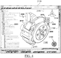
- FIG. 4 shows an example of the GUI of a typical CAD system.
- the GUI 2100 may be a typical CAD-like interface, having standard menu bars 2110, 2120, as well as bottom and side toolbars 2140, 2150.
- Such menu and toolbars contain a set of user-selectable icons, each icon being associated with one or more operations or functions, as known in the art.
- Some of these icons are associated with software tools, adapted for editing and/or working on the 3D modeled object 2000 displayed in the GUI 2100.
- the software tools may be grouped into workbenches. Each workbench comprises a subset of software tools. In particular, one of the workbenches is an edition workbench, suitable for editing geometrical features of the modeled product 2000.
- a designer may for example pre-select a part of the object 2000 and then initiate an operation (e.g. a sculpting operation, or any other operation such as a change of dimension, color, etc.) or edit geometrical constraints by selecting an appropriate icon.
- an operation e.g. a sculpting operation, or any other operation such as a change of dimension, color, etc.
- typical CAD operations are the modeling of the punching or the folding of the 3D modeled object displayed on the screen.
- the GUI may for example display data 2500 related to the displayed product 2000.
- the data 2500, displayed as a "feature tree", and their 3D representation 2000 pertain to a brake assembly including brake caliper and disc.
- the GUI may further show various types of graphic tools 2130, 2070, 2080 for example for facilitating 3D orientation of the object, for triggering a simulation of an operation of an edited product or rendering various attributes of the displayed product 2000.
- a cursor 2060 may be controlled by a haptic device to allow the user to interact with the graphic tools.
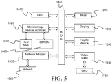
- FIG. 5 shows an example of the architecture of the system as a client computer system, e.g. a workstation of a user.
- the client computer comprises a central processing unit (CPU) 1010 connected to an internal communication BUS 1000, a random access memory (RAM) 1070 also connected to the BUS.
- the client computer is further provided with a graphics processing unit (GPU) 1110 which is associated with a video random access memory 1100 connected to the BUS.
- Video RAM 1100 is also known in the art as frame buffer.
- a mass storage device controller 1020 manages accesses to a mass memory device, such as hard drive 1030.
- Mass memory devices suitable for tangibly embodying computer program instructions and data include all forms of nonvolatile memory, including by way of example semiconductor memory devices, such as EPROM, EEPROM, and flash memory devices; magnetic disks such as internal hard disks and removable disks, magneto-optical disks, and CD-ROM disks 1040. Any of the foregoing may be supplemented by, or incorporated in, specially designed ASICs (application-specific integrated circuits).
- a network adapter 1050 manages accesses to a network 1060.
- the client computer may also include a haptic device 1090 such as a cursor control device, a keyboard or the like.
- a cursor control device is used in the client computer to permit the user to selectively position a cursor at any desired location on screen 1080, as mentioned with reference to FIG. 4 .
- screen it is meant any support on which displaying may be performed, such as a computer monitor.
- the cursor control device allows the user to select various commands, and input control signals.
- the cursor control device includes a number of signal generation devices for input control signals to system.
- a cursor control device may be a mouse, the button of the mouse being used to generate the signals.
- a computer program comprising instructions for execution by a computer, the instructions comprising means for this purpose.
- the program may for example be implemented in digital electronic circuitry, or in computer hardware, firmware, software, or in combinations of them.
- Apparatus of the invention may be implemented in a computer program product tangibly embodied in a machine-readable storage device for execution by a programmable processor; and method steps of the invention may be performed by a programmable processor executing a program of instructions to perform functions of the invention by operating on input data and generating output.
- the instructions may advantageously be implemented in one or more computer programs that are executable on a programmable system including at least one programmable processor coupled to receive data and instructions from, and to transmit data and instructions to, a data storage system, at least one input device, and at least one output device.
- the application program may be implemented in a high-level procedural or object-oriented programming language, or in assembly or machine language if desired; and in any case, the language may be a compiled or interpreted language.
- the program may be a full installation program, or an update program. In the latter case, the program updates an existing CAD system to a state wherein the system is suitable for performing the method.
- the method of FIG. 1 is for designing a 3D modeled object starting from the plurality of 2D views of the modeled object and the corresponding 3D wireframe graph by determining at S30 the edge cycles.
- the edge cycles may then be used, among other possible actions known in the field, for fitting the wireframe graph with surfaces based on them, according to any known method.
- the surfaces may form a boundary representation (B-Rep), e.g. under the specific format of B-Reps described in European patent application No. 12306720.9 (published as EP2750107 ).
- the method may determine at S30 one edge cycle per tile of the wireframe graph (referred to as "minimum edge cycle" in the following), such that the whole set of edge cycles eventually covers the whole wireframe graph, with no overlapping.
- the views that are provided at S10 are any 2D representations of the 3D modeled object that is under design.
- the views may be images.
- the method may notably, prior to the providing S10, capture several images of a same single physical product that may constitute the views, potentially including some modifications/additions on the images, as explained below. This may be done for example by a camera capturing photos. For example, a same physical product may be photographed from different angles, the resulting photos thus representing the product under different perspectives.
- the outer surface of the physical product is integrally represented through the plurality of views.
- the method may in such a case reconstruct, or build, a comprehensive 3D design of the physical product (or in general any object represented by the views), i.e. the 3D modeled object, based on smaller information (2D views) that are however multiple.
- the first step toward this is to consider a 3D wireframe graph that corresponds to the plurality of 2D views in a way explained later.
- the 3D wireframe graph may be provided at S10 already prepared as such, or it may be constructed in a prior step by the method according to any known technique, e.g. based on the 2D views.
- the method may comprise defining curves and points on the images to form the views.
- the views are data including a standard image with 2D curves and 2D points defined thereon.
- the curves and points may be defined, in any known way, according to the images and the lines and corners of the physical product as they appear on the images. The user may be involved in such a step, as explained earlier. Known automatic algorithms may also be used.
- the method comprises defining correspondences (in the case of a computer-implemented method, correspondences are pieces of data that associate two pieces of data, such as links or pointers) between the curves and points of each image with respectively curves and points on the other images.
- correspondences are pieces of data that associate two pieces of data, such as links or pointers
- curves and points of different images that represent the same lines and corners of the physical product are put into correspondence, precisely so as to highlight such information. This may be performed according to any know method. The user may be involved in such a step, as explained earlier. Known automatic algorithms may also be used.
- the 3D wireframe graph is a graph having a specific structure, according to the method.
- the wireframe graph comprises as all graphs edges that connect vertices, and correspondences between the edges and the vertices with respectively curves and points on the views.
- the edges of the 3D wireframe graph are associated with 3D curves (also referred to as the edges in the following) and the vertices of the 3D wireframe graph are associated to 3D points or positions (also referred to as the vertices in the following).
- the wireframe graph is a three-dimensional modeled object.
- the 3D edges and the 3D vertices are determined (when the method comprises constructing the wireframe graph) based on the views and on the correspondences defined earlier. This may be done according to any method known in the art, and this may involve user-interaction and/or known automatic algorithms.
- the wireframe graph is a construction of the modeled object that is based on the images, in the sense that different 2D information on the same physical product contained in the images is used to reconstruct a 3D wireframe graph corresponding to the product, as known per se.
- the physical product may be opaque, such that its lines and corners are well defined and such that there is no ambiguity among the different 2D views.
- the method also comprises associating S20 (i.e. pieces of data representing such association, e.g. links and/or pointers, are created), to each vertex of the wireframe graph, a local radial order between all the edges incident to the vertex.
- S20 i.e. pieces of data representing such association, e.g. links and/or pointers, are created
- S20 i.e. pieces of data representing such association, e.g. links and/or pointers, are created
- S20 i.e. pieces of data representing such association, e.g. links and/or pointers, are created
- S20 i.e. pieces of data representing such association, e.g. links and/or pointers, are created
- the local order is radial, meaning that it represents the order in which the edges are encountered when rotating around the vertex.
- the local radial order may radially order the projections of the edges (e.g. a projection of the tangents of the edges at the incident vertex)
- the associating S20 is performed according to local partial radial orders between the curves corresponding to the edges on each of the views with respect to the point corresponding to the vertex.
- the edges of the wireframe each correspond to a respective curve on at least one of the views. Indeed, according to the perspective applied by a given view, some edges may not be present on it. However, for each edge there is at least one view for which the perspective is such that the view has a curve corresponding to the edge defined thereon. Now, considering the set of edges incident on each contemplated vertex of the associating S20, all the edges are present on at least one of the plurality of views for each of them (via the corresponding 2D curves defined on the views).
- a radial order may be directly defined between said curves, called "local partial radial order", the view being 2D.
- the associating S20 considers all such local partial radial orders that correspond to the set of edges incident on the contemplated vertex and determines the local radial order between all edges accordingly, in a systematic way (e.g. the method may follow a predetermined algorithm to perform the associating), which allows automation. An example of how to implement this is provided later.
- the method uses at S20 the views to determine such local radial orders for all vertices of the wireframe graph, in addition to a potential previous use of the views to determine the wireframe graph. In this sense, the views are efficiently reused for the automation of this part of the process.
- the method comprises determining S30 edge cycles.
- the determining S30 is performed by browsing the wireframe graph following the local radial orders associated at S20 to the vertices.
- the graph is integrally traversed (i.e. edges are followed until all tiles of the wireframe graph are cycled once) following the local radial orders.
- the method may store the orders in which the edges are thereby followed and define instances of cycles (each time the browsing leads to a vertex already visited). This is illustrated later.
- the determining S30 is thus executable in a systematic way and may thus lead to a significant automation of the determination of the edge cycles, in a relatively simple manner (in terms of computation and memory resources).
- Said edge cycles may be used to fit the wireframe graph with surfaces, e.g. a B-Rep, as explained earlier.
- FIG. 6 showing a flowchart representing the whole method of the discussed example.
- the physical product of the example to model in the CAD system is L-shape solid 60.
- the internal edge of the "L” is filleted.
- the user feeds at S05 the CAD system with five 2D pictures (e.g. photos) of this solid ( FIGS. 7-11 ) captured at S05, on which curves and points are defined. Camera positions associated with pictures are also sent to the CAD system in the example.
- the next step of the method of the example is for the user to define and match up at S06 and S07 points across overlapping pictures (curves being matched up accordingly).
- the resulting views are illustrated on FIGS. 12-16 by numerical labels which respectively correspond to the five pictures of FIGS. 7-11 . Points are numbered from 1 to 14. Points are tagged with their number on the figures where they are visible.
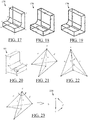
- the CAD system is able to compute at S08 a network of 3D curves (the edges), in other words 3D wireframe graph 170 as illustrated in FIG. 17 .
- the state of the art technology is able to compute this 3D wireframe graph.
- Each vertex and each edge on the 3D wireframe graph corresponds to a point and curve that are each visible on at least two input pictures. It is indeed advantageous to retrieve the 3D position and shape of an object from more than one 2D view/picture of the said object.
- a goal of the method of the example is to eventually compute all minimum edge cycles of this graph at S30, so that the surfaces boundary may potentially be defined according to known algorithms.
- a "minimum edge cycle" is defined as follows. When projected on initial pictures, oriented edges of the same minimum cycle correspond to boundary curves of the same 2D face.
- a planar simple loop (loop) in the following) is a planar closed curve that separates the plane into exactly two portions.
- the non-bounded portion is named the "outside” of the loop and the bounded portion is named the "inside” of the loop.
- a planar face includes one loop named the "external loop” and a set of loops named “internal loops”.
- the external loop is mandatory while internal loops are not.
- Loops are arranged according to the following conditions:
- FIG. 18 illustrates five such minimum edge cycles.
- FIG. 19 illustrates a cycle that is not a minimum cycle: some edges are boundary curves of the bottom face of the L-shape solid while some others are boundary edges of the back face of the L-shape solid.
- the method computes all minimum edge cycles through two steps.
- the first step is to sort edges around each vertex according to an appropriate topological local radial order at S20.
- the second step is to traverse the 3D graph by using these radial orderings at S30.
- the method of the example provides a strategy ("regularize" step S28 on FIG. 6 discussed later) to overcome the difficulty that is reasonably efficient in industrial situations.
- the associating S20, to each vertex of the wireframe graph, of a local radial order between all the edges incident to a respective vertex comprises specific actions for each respective vertex that are easily automatable and lead to fairly good results.
- the associating S20 comprises for each respective vertex determining S22, for each view, the local partial radial order with respect to the point corresponding to the respective vertex between curves that are defined on the view and that correspond to an edge incident to the respective vertex.
- the method considers 2D curves on the 2D views that correspond to the edges incident to the respective vertex and determines at S22 radial orders thereof on each view. Then, the method performs a merging S24 of all the local partial radial orders.
- the method traverses at S26 the result of the merging S24 (edges of the merge graph are followed), to detect a cycle (one or more) including all the edges incident to the respective vertex, said cycle constituting the local radial order associated to the respective vertex.
- the local partial radial orders are determined at S22 as graphs of which nodes identify edges and of which arcs identify subsequence between edges (i.e. two edges that are subsequent one to the other on the wireframe graph are linked by an oriented arc on the "local partial order" graphs).
- Ordering incident edges of a vertex x is performed through two steps.
- the first step is to gather at S22 and S24 around vertex x all partial radial orders computed from pictures where it is visible.
- the second step is to extract at S26 (and possibly S28) from all these partial radial orders a unique local radial order.
- the method of the example finds all views where it is visible. For each such view, the method gets the visible edges incident to x , sorts these edges around vertex x in a predetermined order (e.g. CCW: counter clockwise) induced by the planar topology of the picture and stores this partial order in an appropriate data structure.
- a predetermined order e.g. CCW: counter clockwise
- vertex 12 of solid 60 is connected to edges (12,5), (12,11) and (12,13).
- the view of FIGS. 8 and 13 features vertex 12 together with all its connected edges which, additionally, are visible.
- the CCW radial order is then: ((12,5),(12,13),(12,11)) as illustrated in FIG. 20 .
- each vertex is visible together with all its incident edges from at least one picture, which particularly simplifies the radial order computation (because the merging S24 will lead to a uniquely ordered cycle).
- FIGS. 21-26 illustrate a case where the merging S24 and the traversing S26 help combining the information determined at S22.
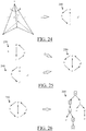
- FIGS. 21-22 illustrate two pictures of a pyramidal V-based solid. Edges a,b,c,d are incident to the top vertex v of the pyramid. Dotted lines are invisible edges, they should not appear on the pictures, but they are represented for explanation purpose.
- vertex v is visible together with incident edges a,c,d, edge b being hidden.
- the partial local radial order 230 is then ( a,c,d ) , as illustrated in FIG. 23 .
- vertex v is visible together with incident edges a,b,c, edge d being hidden.
- the partial local radial 240 order is then ( a,b,c ) , as illustrated in FIG. 24 .
- the local radial order is obtained at S20 by combining and analyzing at S26 local partial radial orders.
- vertex v is associated with local partial radial orders ( a,c,d ) and ( a,b,c ) .
- the first step is to merge at S26 all local partial radial orders into a single graph 250, as illustrated on FIG. 25 . It must be understood that the vertices a,b,c,d of partial radial order graphs are edges of the 3D wireframe graph and that oriented arcs of partial radial order graphs capture partial radial orders around vertex v.
- FIG. 26 illustrates the graph traversal starting from node a , which yields a tree 260 rooted at node a .
- graph traversal is interrupted when a node of the current branch is previously visited (a branch being a path of arcs starting at the root node).
- the resulting rooted tree 260 is illustrated in FIG. 26 .
- Tree 260 collects all cycles of the graph as follows: each path from the root node to a leaf node is a cycle. It is clear in this example that there exists only one maximum cycle which is ( a,b,c,d ) and illustrated with boxed letters. This cycle is the local radial order of edges around vertex v retained by the method of the example. It may happen that the maximum cycle is not unique, thus leading to ambiguity. This situation is detailed later.
- determining (S30) edge cycles by browsing the wireframe graph comprises the sub-steps of chosing a vertex and forming an edge list starting from the chosen vertex, and repeating said sub-steps.
- vertices are repeatedly chosen and edge lists are formed each time a vertex is chosen, e.g. until all minimal edge lists are determined.
- Forming the edge list is performed by following, starting from the chosen vertex, the local radial orders associated to the vertices as they are encountered.
- the algorithm retrieves the first edge provided by the local radial order associated to said vertex (e.g. the method marks edges of the local radial orders as used, such that the algorithm retrieves the first unused edge of the local radial order).
- the algorithm goes to the other vertex connected to said edge.
- the algorithm increments the edge list with such followed edges, until the edge list forms an edge cycle. This allows a fast and efficient determination at S30.
- determining S30 edge cycles by browsing the wireframe graph comprises the sub-steps of:
- the input data for 3D wireframe graph traversal are the 3D wireframe graph together with local radial orders at each vertex.
- the output data is the list of all minimum cycles of the 3D graph.
- the following preprocessing is advantageous: all edges of the 3D graph are duplicated and oriented in opposite directions. By definition, an oriented edge is "used” if it is involved in a minimum cycle. A vertex is “used” if all its output edges are used in minimum cycles. Before the algorithm starts, all edges and all vertices are "unused”. At the end of the algorithm, each oriented edge is involved in one and only one minimum cycle.
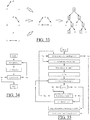
- the graph traversal algorithm is described in the diagram of FIG. 27 .
- the method takes advantage of the local radial orders so that, with a simple but smart marking of vertices and edges as used or unused (after the duplication), the method may easily and efficiently perform the determination S30 of all minimal edge cycles.
- a non-unique local radial order may occur as explained in the following.
- the example solid is a tetrahedron, as illustrated on FIG. 28 .
- Four pictures of the tetrahedron are given in such a way that only one face is visible on each picture. Each visible face hides all three other faces of the tetrahedron, as illustrated by FIG. 29 .
- the method of the example may solve this issue by selecting S28 one of the cycles detected for such a vertex having several different local radial orders (potentially) associated to it, and referred to as "singular" vertex.
- the method thus selects one cycle as the local radial order used in the determining S30.
- the method may further comprise marking the vertex as a singular vertex (after the traversal S26), for later use of such information.
- the selecting S28 may be performed indirectly.
- the selecting S28 one of the cycles detected may indeed comprise performing a regularization process (which is iterative) on the set of all singular vertices.
- the regularization process comprises chosing a starting singular vertex and a starting output edge (an edge incident to the chosen singular vertex) of said starting singular vertex. This chosing may be performed in any way. Then the regularization process comprises browsing the wireframe graph following the local radial orders associated to the vertices (i.e. the first edge of the local radial order associated to an edge is followed each time the algorithm arrives at a vertex), in order to detect an edge cycle at said starting singular vertex.
- the method repeats the regularization process with a new starting singular vertex and/or a new starting output edge (the browsing is indeed facing an ambiguity and the proposed way to solve this ambiguity is to restart somewhere else).
- the method may associate to said starting singular vertex the cycle, that was detected at S26, and that is compliant with the order between the starting output edge and the final edge browsed (the other potential local radial order(s) that are provided by the other cycles detected at S26 in competition are discarded).
- the local radial order that is retained is the one in which the starting edge and the ending edge of the cycle detected during the regularization (both edges being incident to the singular vertex under regularization) are ordered correctly (i.e. in the same order as for the detected cycle). Then the method removes the starting singular vertex from the set of all singular vertices (indeed, the singular vertex has been regularized as a unique local radial order has been retained for it), and then repeats the regularization process. This algorithm is executed until no singular vertex remains. Examples are discussed hereunder.
- a vertex featuring a non-unique local radial order is called a singular vertex in the following.
- the principle is as follows. Suppose that all possible local radial orders are computed and start a cycle computation at a singular vertex x. Since the starting edge of the cycle, noted u, is arbitrarily chosen among output edges of x, singularity is not a trouble. If no other singular vertex is encountered while computing the cycle, the algorithm ends the said cycle with an edge v that is an input edge of vertex x. So, it is clear that the appropriate radial order around vertex x is the one featuring the sequence u,v as opposed to the one featuring the sequence v,u. Consequently, it is possible to regularize vertex x by setting the correct local radial order. Then, the strategy is to identify singular vertices while computing local radial orders and to regularize them as much as possible.
- the regularization algorithm is as shown on FIG. 34 . After local radial orders are computed, all singular vertices are stored in an initial list L . The main loop is to iteratively remove singular vertices from list L . Iterations are stopped when no singular vertex can be removed.
- the resulting list is not empty, it includes unavoidable singular vertices and cycle computation is not possible. Otherwise, all singular vertices are removed and all local radial orders are unique. The cycles computation described previously will be successful.
- Function Reg( L ) tries to regularize each singular vertex of the input list L . It modifies list L by removing elements and decreasing its size. If at least one vertex is regularized, there is a chance that a new try regularizes some others, which validates iterations.
- Function Reg( L ) is as follows:
- Regularizing vertex x in function Reg( L ) is to search a cycle starting at vertex x including only regular vertices but x . This is performed as described in the diagram of FIG. 35 .
- FIGS. 37-39 illustrate three input images of solid 360 of FIG. 36 . Notice that hidden lines are represented as dotted lines for clarity and should not appear on images. Vertex 4 is not visible on the image of FIG. 37 . Vertex 3 is not visible on the image of FIG. 38 . Vertex 2 is not visible on the image of FIG. 39 .
- Computed local radial orders are illustrated on FIG. 40 .
- Vertices 1 and 5 are singular since radial orders could not be oriented. It should be noticed that initializing a cycle computation at a regular vertex always fails because any cycle include either vertex 1 or vertex 5, which are singular so far.
- the list of singular vertices includes 1 and 5. Regularization starts with vertex 1. Choosing edge (1,3) leads to vertex 3, which is regular. Thanks to local ordering at vertex 3, next edge is (3,4) leading to vertex 4, which is regular. Thanks to local ordering at vertex 4, next edge is (4,1) closing the cycle at vertex 1. Clearly, the appropriate local ordering at vertex 1 is (1,3),(1,4),(1,2) changing it into a regular vertex. Singular vertex 5 is regularized the same way. Then, computation of all cycles is possible.
- V,E respectively the number of vertices and edges of the 3D wireframe graph and F the number of faces of the input object, which is also the number of minimum cycles.
- E max the largest number of edges incident to a vertex.
- E max can be made proportional to E with particular solids, real life objects feature a small and constant E max .
- the algorithmic complexity of graph traversal is proportional to E since each edge is visited twice.
- the overall complexity of the algorithm is linear, meaning that it is proportional to aE + bV where a,b are constant numbers.
Landscapes
- Engineering & Computer Science (AREA)
- Physics & Mathematics (AREA)
- Theoretical Computer Science (AREA)
- Geometry (AREA)
- General Physics & Mathematics (AREA)
- Software Systems (AREA)
- Computer Graphics (AREA)
- Evolutionary Computation (AREA)
- Computer Hardware Design (AREA)
- General Engineering & Computer Science (AREA)
- Computational Mathematics (AREA)
- Mathematical Analysis (AREA)
- Mathematical Optimization (AREA)
- Pure & Applied Mathematics (AREA)
- Image Generation (AREA)
- Processing Or Creating Images (AREA)
- Architecture (AREA)
Claims (13)
- Computerimplementiertes Verfahren zum Entwurf eines dreidimensional modellierten Gegenstands, umfassend die folgenden Schritte:• Bereitstellen (S10) einer Vielzahl von zweidimensionalen Ansichten des modellierten Gegenstands mit darauf definierten Kurven und Punkten eines dreidimensionalen Drahtgittergraphen, umfassend Kanten, die Scheitel verbinden, und Korrespondenzen zwischen den Kanten und den Scheiteln mit entsprechenden Kurven und Punkten auf den Ansichten,• Assoziieren (S20), mit jedem Scheitel des Drahtgittergraphen, einer lokalen radialen Ordnung zwischen allen Kanten, die auf den Scheitel zulaufen, gemäß teilweisen lokalen radialen Ordnungen zwischen den Kurven, die den Kanten auf jeder der Ansichten mit Bezug auf den Punkt entsprechen, der dem Scheitel entspricht, und dann• Bestimmen (S30) von Kantenzyklen durch Durchsuchen des Drahtgittergraphen gemäß den lokalen radialen Ordnungen, die mit den Scheiteln assoziiert sind.
- Verfahren nach Anspruch 1, wobei das Assoziieren (S20), mit jedem Scheitel des Drahtgittergraphen, einer lokalen radialen Ordnung zwischen allen Kanten, die auf einen entsprechenden Scheitel zulaufen, für jeden entsprechenden Scheitel Folgendes umfasst:• Bestimmen (S22), für jede Ansicht, der lokalen teilweisen radialen Ordnung mit Bezug auf den Punkt, der dem entsprechenden Scheitel zwischen den Kurven entspricht, die auf der Ansicht definiert sind, und die einer Kante, die auf den entsprechenden Scheitel zuläuft, entsprechen,• Mischen (S24) aller lokalen teilweisen radialen Ordnungen, und• Durchlaufen (S26) des Ergebnisses des Mischens (S24) aller lokalen teilweisen radialen Ordnungen, um einen Zyklus nachzuweisen, darin eingeschlossen alle Kanten, die auf den entsprechenden Scheitel zulaufen, wobei der Zyklus die lokale radiale Ordnung darstellt, die mit dem entsprechenden Scheitel assoziiert ist.
- Verfahren nach Anspruch 2, wobei die lokalen teilweisen radialen Ordnungen als Grahpen bestimmt (S22) sind, von denen Knoten Kanten identifizieren, und von denen Bögen eine Aufeinanderfolge zwischen Kanten identifizieren.
- Verfahren nach Anspruch 2 oder 3, wobei das Assoziieren (S20), mit jedem Scheitel auf dem Drahtgittergraphen, einer lokalen radialen Ordnung zwischen allen Kanten, die auf einen entsprechenden Scheitel zulaufen, beim Durchlaufen (S26) des Ergebnisses des Mischens (S24) aller lokalen teilweisen radialen Ordnungen, zum Nachweis von mehreren Zyklen führt, darin eingeschlossen alle Kanten, die auf den entsprechenden Scheitel zulaufen, die Auswahl (S28) eines der Zyklen, die für den entsprechenden Scheitel nachgewiesen wurden, wobei der entsprechende Scheitel ein singulärer Scheitel ist.
- Verfahren nach Anspruch 4, wobei das Auswählen (S28) eines der nachgewiesenen Zyklen das Durchführen eines Regularisierungsprozesses auf dem Satz von singulären Scheitel umfasst, wobei der Regularisierungsprozess Folgendes umfasst:• Wählen eines singulären Ausgangsscheitels und einer Ausgangsausgabekante des singulären Ausgangsscheitels,• Durchsuchen des Drahtgittergraphen gemäß den lokalen radialen Ordnungen, die mit den Scheiteln assoziiert sind, um einen Kantenzyklus an dem singulären Ausgangsscheitel nachzuweisen, und• dann:∘ wenn ein weiterer singulärer Scheitel erreicht wird, Wiederholen des Regularisierungsprozesses mit einem neuen singulären Ausgangsscheitel und/oder einer neuen Ausgangsausgabekante,∘ andernfalls Assoziieren mit dem singulären Ausgangsscheitel des Zyklus, der nachgewiesen wurde beim Durchlaufen (S26) des Ergebnisses des Mischens (S24) aller lokalen teilweisen radialen Ordnungsführungen, das mit der Ordnung zwischen dem Ausgangsausgabekante und der durchsuchten Letztekante übereinstimmt, Entfernen des singulären Ausgangsscheitels vom Satz aller singulären Scheitel, und dann Wiederholen des Regularisierungsprozesses, bis kein singulärer Scheitel zurückbleibt.
- Verfahren nach einem der Ansprüche 1 - 5, wobei das Bestimmen (S30) von Kantenzyklen durch Durchsuchen des Drahtgittergraphen die folgenden Unterschritte umfasst:• Wählen eines Scheitels,• Bilden einer Kantenliste, folgend, ausgehend vom gewählten Scheitel, der lokalen radialen Ordnungen, die mit den Scheiteln assoziiert sind, wenn sie angetroffen werden und Erweitern der Kantenliste mit den gefolgten Kanten, bis die Kantenliste einen Kantenzyklus bildet, und• Wiederholen der vorhergehenden Unterschritte.
- Verfahren nach einem der Ansprüche 1 - 6, wobei die Ansichten Bilder sind und der Drahtgittergraph eine dreidimensionale Konstruktion des modellierten Gegenstands, basierend auf den Bildern, ist.
- Verfahren nach Anspruch 7, wobei das Verfahren weiter, vor dem Bereitstellen (S10) der Ansichten, des Drahtgittergraphen und der Korrespondenzen, Folgendes umfasst:• Erfassen (S05) von Bildern eines gleichen physischen Produkts,• Definieren (S06) von Kurven und Punkten auf den Bildern, dadurch Bilden der Ansichten,• Definieren (S07) Korrespondenzen zwischen den Kurven und Punkten jedes Bildes mit entsprechenden Kurven und Punkten auf den anderen Bildern, und• Konstruieren (S08) des Drahtgittergraphen basierend auf den Ansichten und den Korrespondenzen, wobei der dadurch konstruierte Drahtgittergraph Kanten umfasst, die Scheitel verbinden, und Korrespondenzen zwischen den Kanten und den Scheiteln mit entsprechenden Kurven und Punkten auf den Ansichten.
- Verfahren nach Anspruch 7 oder 8, wobei die Bilder Photos sind.
- Verfahren nach einem der Ansprüche 1 - 9, weiter umfassend Ausstatten des Drahtgittergraphen mit Flächen basierend auf den bestimmten Kantenzyklen.
- Computerprogramm, umfassend Anweisungen zum Durchführen des Verfahrens nach einem der Ansprüche 1 - 10.
- Datenspeichermedium, auf dem das Computerprogramm nach Anspruch 11 aufgezeichnet ist.
- CAD-System, umfassend einen Prozessor, der mit einem Speicher und einer graphischen Benutzerschnittstelle gekoppelt ist, wobei auf dem Speicher das Computerprogramm nach Anspruch 11 aufgezeichnet ist.
Priority Applications (6)
| Application Number | Priority Date | Filing Date | Title |
|---|---|---|---|
| EP13305751.3A EP2811463B1 (de) | 2013-06-04 | 2013-06-04 | Entwurf eines 3D-modellierten Objekts mit 2D-Ansichten |
| US14/290,639 US9886528B2 (en) | 2013-06-04 | 2014-05-29 | Designing a 3D modeled object with 2D views |
| CA2853255A CA2853255A1 (en) | 2013-06-04 | 2014-05-30 | Designing a 3d modeled object with 2d views |
| CN201410380379.3A CN104217066B (zh) | 2013-06-04 | 2014-06-03 | 利用2d视图设计3d建模对象 |
| JP2014115172A JP6498872B2 (ja) | 2013-06-04 | 2014-06-03 | 2dビューを用いた3dモデル化オブジェクトの設計 |
| KR1020140067954A KR20140142679A (ko) | 2013-06-04 | 2014-06-03 | 2차원 뷰들로 3차원 모델링된 오브젝트의 설계 |
Applications Claiming Priority (1)
| Application Number | Priority Date | Filing Date | Title |
|---|---|---|---|
| EP13305751.3A EP2811463B1 (de) | 2013-06-04 | 2013-06-04 | Entwurf eines 3D-modellierten Objekts mit 2D-Ansichten |
Publications (3)
| Publication Number | Publication Date |
|---|---|
| EP2811463A1 EP2811463A1 (de) | 2014-12-10 |
| EP2811463A8 EP2811463A8 (de) | 2015-02-18 |
| EP2811463B1 true EP2811463B1 (de) | 2018-11-21 |
Family
ID=49115453
Family Applications (1)
| Application Number | Title | Priority Date | Filing Date |
|---|---|---|---|
| EP13305751.3A Active EP2811463B1 (de) | 2013-06-04 | 2013-06-04 | Entwurf eines 3D-modellierten Objekts mit 2D-Ansichten |
Country Status (6)
| Country | Link |
|---|---|
| US (1) | US9886528B2 (de) |
| EP (1) | EP2811463B1 (de) |
| JP (1) | JP6498872B2 (de) |
| KR (1) | KR20140142679A (de) |
| CN (1) | CN104217066B (de) |
| CA (1) | CA2853255A1 (de) |
Families Citing this family (19)
| Publication number | Priority date | Publication date | Assignee | Title |
|---|---|---|---|---|
| EP2874118B1 (de) | 2013-11-18 | 2017-08-02 | Dassault Systèmes | Berechnung von Kameraparametern |
| EP3032495B1 (de) | 2014-12-10 | 2019-11-13 | Dassault Systèmes | Texturierung eines 3D-modellierten Objekts |
| CN104899925A (zh) * | 2015-06-29 | 2015-09-09 | 遵义宏港机械有限公司 | 一种数控铣床工件三维建模方法 |
| EP3188033B1 (de) | 2015-12-31 | 2024-02-14 | Dassault Systèmes | Rekonstruktion eines 3d-modellierten objekts |
| EP3200160B1 (de) * | 2016-01-29 | 2018-12-19 | Dassault Systèmes | Computerimplementiertes verfahren zum design eines dreidimensionalen, modellierten objekts mit einer kurve und einer stelle auf der kurve |
| US10587858B2 (en) * | 2016-03-14 | 2020-03-10 | Symbol Technologies, Llc | Device and method of dimensioning using digital images and depth data |
| CN106125907B (zh) * | 2016-06-13 | 2018-12-21 | 西安电子科技大学 | 一种基于线框模型的三维目标注册定位方法 |
| CN106530388A (zh) * | 2016-09-08 | 2017-03-22 | 上海术理智能科技有限公司 | 一种基于二维图像的3d打印装置及其三维建模方法 |
| EP3293705B1 (de) | 2016-09-12 | 2022-11-16 | Dassault Systèmes | 3d-rekonstruktion eines realen objekts aus einer tiefenkarte |
| JP2018067115A (ja) * | 2016-10-19 | 2018-04-26 | セイコーエプソン株式会社 | プログラム、追跡方法、追跡装置 |
| US11244502B2 (en) * | 2017-11-29 | 2022-02-08 | Adobe Inc. | Generating 3D structures using genetic programming to satisfy functional and geometric constraints |
| KR101988372B1 (ko) * | 2018-11-30 | 2019-06-12 | 주식회사 큐픽스 | 사진 이미지를 이용한 3차원 건축물 모델 역설계 장치 및 방법 |
| EP3675063B1 (de) * | 2018-12-29 | 2026-02-11 | Dassault Systèmes | Herstellung eines datensatzes zur inferenz von festen cad-merkmalen |
| EP3675062A1 (de) | 2018-12-29 | 2020-07-01 | Dassault Systèmes | Lernen eines neuronalen netzwerks zur inferenz von soliden cad-merkmalen |
| US12400044B2 (en) * | 2020-02-13 | 2025-08-26 | Mitsubishi Electric Corporation | Dimension creation device, dimension creation method, and recording medium |
| EP3958182B1 (de) * | 2020-08-20 | 2025-07-30 | Dassault Systèmes | Variationsautocodierer zur ausgabe eines 3d-modells |
| CN112381921B (zh) * | 2020-10-27 | 2024-07-12 | 新拓三维技术(深圳)有限公司 | 一种边缘重建方法及系统 |
| CN112699426B (zh) * | 2020-12-09 | 2024-08-23 | 深圳微步信息股份有限公司 | 一种io挡板设计方法、io挡板 |
| CN116805306A (zh) * | 2023-06-28 | 2023-09-26 | 网易(杭州)网络有限公司 | 模型拓扑检测方法、装置、电子设备及存储介质 |
Family Cites Families (32)
| Publication number | Priority date | Publication date | Assignee | Title |
|---|---|---|---|---|
| JPH07120410B2 (ja) * | 1991-01-15 | 1995-12-20 | インターナショナル・ビジネス・マシーンズ・コーポレイション | 大規模並列アーキテクチャによる3次元物体の表示・操作システム及び方法 |
| JP3162630B2 (ja) * | 1996-07-31 | 2001-05-08 | トヨタ自動車株式会社 | ワイヤフレームモデルの面定義方法および装置 |
| US6549201B1 (en) * | 1999-11-23 | 2003-04-15 | Center For Advanced Science And Technology Incubation, Ltd. | Method for constructing a 3D polygonal surface from a 2D silhouette by using computer, apparatus thereof and storage medium |
| US7084868B2 (en) | 2000-04-26 | 2006-08-01 | University Of Louisville Research Foundation, Inc. | System and method for 3-D digital reconstruction of an oral cavity from a sequence of 2-D images |
| US6654027B1 (en) * | 2000-06-09 | 2003-11-25 | Dassault Systemes | Tool for three-dimensional analysis of a drawing |
| US6834119B2 (en) | 2001-04-03 | 2004-12-21 | Stmicroelectronics, Inc. | Methods and apparatus for matching multiple images |
| US6850233B2 (en) | 2002-05-01 | 2005-02-01 | Microsoft Corporation | Systems and methods for optimizing geometric stretch of a parametrization scheme |
| US6825838B2 (en) * | 2002-10-11 | 2004-11-30 | Sonocine, Inc. | 3D modeling system |
| US7546156B2 (en) | 2003-05-09 | 2009-06-09 | University Of Rochester Medical Center | Method of indexing biological imaging data using a three-dimensional body representation |
| WO2007146069A2 (en) * | 2006-06-07 | 2007-12-21 | Carnegie Mellon University | A sketch-based design system, apparatus, and method for the construction and modification of three-dimensional geometry |
| KR100969764B1 (ko) | 2008-02-13 | 2010-07-13 | 삼성전자주식회사 | 메쉬 모델로 구현된 3차원 데이터의 부호화 및 복호화 방법 |
| US8570343B2 (en) | 2010-04-20 | 2013-10-29 | Dassault Systemes | Automatic generation of 3D models from packaged goods product images |
| KR101696918B1 (ko) | 2010-05-11 | 2017-01-23 | 톰슨 라이센싱 | 3차원 비디오를 위한 컴포트 노이즈 및 필름 그레인 처리 |
| EP2400410B1 (de) * | 2010-05-25 | 2014-01-08 | Dassault Systèmes | Berechnung einer resultierenden dreieckigen vielflächigen Oberfläche von einem ersten und einem zweiten modellierten Objekt |
| JP6057298B2 (ja) | 2010-10-07 | 2017-01-11 | サンジェビティ | 迅速な3dモデリング |
| US9235891B2 (en) | 2011-01-10 | 2016-01-12 | Rutgers, The State University Of New Jersey | Boosted consensus classifier for large images using fields of view of various sizes |
| US9031356B2 (en) | 2012-03-20 | 2015-05-12 | Dolby Laboratories Licensing Corporation | Applying perceptually correct 3D film noise |
| US9218685B2 (en) | 2012-06-05 | 2015-12-22 | Apple Inc. | System and method for highlighting a feature in a 3D map while preserving depth |
| CN104395929B (zh) | 2012-06-21 | 2017-10-03 | 微软技术许可有限责任公司 | 使用深度相机的化身构造 |
| US9183666B2 (en) | 2013-03-15 | 2015-11-10 | Google Inc. | System and method for overlaying two-dimensional map data on a three-dimensional scene |
| US9483703B2 (en) | 2013-05-14 | 2016-11-01 | University Of Southern California | Online coupled camera pose estimation and dense reconstruction from video |
| US9378576B2 (en) | 2013-06-07 | 2016-06-28 | Faceshift Ag | Online modeling for real-time facial animation |
| EP2874118B1 (de) | 2013-11-18 | 2017-08-02 | Dassault Systèmes | Berechnung von Kameraparametern |
| US9524582B2 (en) | 2014-01-28 | 2016-12-20 | Siemens Healthcare Gmbh | Method and system for constructing personalized avatars using a parameterized deformable mesh |
| US9299195B2 (en) | 2014-03-25 | 2016-03-29 | Cisco Technology, Inc. | Scanning and tracking dynamic objects with depth cameras |
| US9613298B2 (en) | 2014-06-02 | 2017-04-04 | Microsoft Technology Licensing, Llc | Tracking using sensor data |
| US10719727B2 (en) | 2014-10-01 | 2020-07-21 | Apple Inc. | Method and system for determining at least one property related to at least part of a real environment |
| US10110881B2 (en) | 2014-10-30 | 2018-10-23 | Microsoft Technology Licensing, Llc | Model fitting from raw time-of-flight images |
| EP3032495B1 (de) | 2014-12-10 | 2019-11-13 | Dassault Systèmes | Texturierung eines 3D-modellierten Objekts |
| CN104794722A (zh) | 2015-04-30 | 2015-07-22 | 浙江大学 | 利用单个Kinect计算着装人体三维净体模型的方法 |
| EP3188033B1 (de) | 2015-12-31 | 2024-02-14 | Dassault Systèmes | Rekonstruktion eines 3d-modellierten objekts |
| CN105657402B (zh) | 2016-01-18 | 2017-09-29 | 深圳市未来媒体技术研究院 | 一种深度图恢复方法 |
-
2013
- 2013-06-04 EP EP13305751.3A patent/EP2811463B1/de active Active
-
2014
- 2014-05-29 US US14/290,639 patent/US9886528B2/en active Active
- 2014-05-30 CA CA2853255A patent/CA2853255A1/en not_active Abandoned
- 2014-06-03 KR KR1020140067954A patent/KR20140142679A/ko not_active Withdrawn
- 2014-06-03 CN CN201410380379.3A patent/CN104217066B/zh active Active
- 2014-06-03 JP JP2014115172A patent/JP6498872B2/ja active Active
Non-Patent Citations (1)
| Title |
|---|
| None * |
Also Published As
| Publication number | Publication date |
|---|---|
| JP2014235756A (ja) | 2014-12-15 |
| EP2811463A1 (de) | 2014-12-10 |
| JP6498872B2 (ja) | 2019-04-10 |
| CN104217066A (zh) | 2014-12-17 |
| CN104217066B (zh) | 2019-05-14 |
| US9886528B2 (en) | 2018-02-06 |
| CA2853255A1 (en) | 2014-12-04 |
| KR20140142679A (ko) | 2014-12-12 |
| EP2811463A8 (de) | 2015-02-18 |
| US20140358496A1 (en) | 2014-12-04 |
Similar Documents
| Publication | Publication Date | Title |
|---|---|---|
| EP2811463B1 (de) | Entwurf eines 3D-modellierten Objekts mit 2D-Ansichten | |
| CA2838282C (en) | Geometrical elements transformed by rigid motions | |
| EP2750107B1 (de) | Gruppen von gesichtern, die ein geometrisches muster bilden | |
| CN104346769B (zh) | 三维建模对象的压缩 | |
| US9881388B2 (en) | Compression and decompression of a 3D modeled object | |
| JP6125747B2 (ja) | データベースとインタラクションを行うcadシステムのセッション内のモデル化オブジェクトの設計 | |
| JP6039231B2 (ja) | 三次元シーンにおけるオブジェクトの三次元モデル化アセンブリの設計 | |
| CN107067473A (zh) | 对3d建模对象进行重构 | |
| JP6585423B2 (ja) | 順次更新の実行 | |
| US10409921B2 (en) | Designing industrial products by using geometries connected by geometrical constraints | |
| JP2016045967A (ja) | 順次更新の実行 | |
| KR20140147761A (ko) | 접히는 시트 오브젝트의 설계 |
Legal Events
| Date | Code | Title | Description |
|---|---|---|---|
| PUAI | Public reference made under article 153(3) epc to a published international application that has entered the european phase |
Free format text: ORIGINAL CODE: 0009012 |
|
| 17P | Request for examination filed |
Effective date: 20130604 |
|
| AK | Designated contracting states |
Kind code of ref document: A1 Designated state(s): AL AT BE BG CH CY CZ DE DK EE ES FI FR GB GR HR HU IE IS IT LI LT LU LV MC MK MT NL NO PL PT RO RS SE SI SK SM TR |
|
| AX | Request for extension of the european patent |
Extension state: BA ME |
|
| RIN1 | Information on inventor provided before grant (corrected) |
Inventor name: RAMEAU, JEAN-FRANCOIS Inventor name: CLOUX, JONATHAN Inventor name: FAUCHET, ALAIN |
|
| RIN1 | Information on inventor provided before grant (corrected) |
Inventor name: RAMEAU, JEAN-FRANCOIS Inventor name: CLOUX, JONATHAN Inventor name: FAUCHET, ALAIN |
|
| R17P | Request for examination filed (corrected) |
Effective date: 20150610 |
|
| RBV | Designated contracting states (corrected) |
Designated state(s): AL AT BE BG CH CY CZ DE DK EE ES FI FR GB GR HR HU IE IS IT LI LT LU LV MC MK MT NL NO PL PT RO RS SE SI SK SM TR |
|
| GRAP | Despatch of communication of intention to grant a patent |
Free format text: ORIGINAL CODE: EPIDOSNIGR1 |
|
| STAA | Information on the status of an ep patent application or granted ep patent |
Free format text: STATUS: GRANT OF PATENT IS INTENDED |
|
| INTG | Intention to grant announced |
Effective date: 20180727 |
|
| GRAS | Grant fee paid |
Free format text: ORIGINAL CODE: EPIDOSNIGR3 |
|
| GRAA | (expected) grant |
Free format text: ORIGINAL CODE: 0009210 |
|
| STAA | Information on the status of an ep patent application or granted ep patent |
Free format text: STATUS: THE PATENT HAS BEEN GRANTED |
|
| AK | Designated contracting states |
Kind code of ref document: B1 Designated state(s): AL AT BE BG CH CY CZ DE DK EE ES FI FR GB GR HR HU IE IS IT LI LT LU LV MC MK MT NL NO PL PT RO RS SE SI SK SM TR |
|
| REG | Reference to a national code |
Ref country code: CH Ref legal event code: EP |
|
| REG | Reference to a national code |
Ref country code: IE Ref legal event code: FG4D |
|
| REG | Reference to a national code |
Ref country code: DE Ref legal event code: R096 Ref document number: 602013047036 Country of ref document: DE |
|
| REG | Reference to a national code |
Ref country code: AT Ref legal event code: REF Ref document number: 1068432 Country of ref document: AT Kind code of ref document: T Effective date: 20181215 |
|
| REG | Reference to a national code |
Ref country code: SE Ref legal event code: TRGR |
|
| REG | Reference to a national code |
Ref country code: NL Ref legal event code: MP Effective date: 20181121 |
|
| REG | Reference to a national code |
Ref country code: AT Ref legal event code: MK05 Ref document number: 1068432 Country of ref document: AT Kind code of ref document: T Effective date: 20181121 |
|
| PG25 | Lapsed in a contracting state [announced via postgrant information from national office to epo] |
Ref country code: ES Free format text: LAPSE BECAUSE OF FAILURE TO SUBMIT A TRANSLATION OF THE DESCRIPTION OR TO PAY THE FEE WITHIN THE PRESCRIBED TIME-LIMIT Effective date: 20181121 Ref country code: AT Free format text: LAPSE BECAUSE OF FAILURE TO SUBMIT A TRANSLATION OF THE DESCRIPTION OR TO PAY THE FEE WITHIN THE PRESCRIBED TIME-LIMIT Effective date: 20181121 Ref country code: LV Free format text: LAPSE BECAUSE OF FAILURE TO SUBMIT A TRANSLATION OF THE DESCRIPTION OR TO PAY THE FEE WITHIN THE PRESCRIBED TIME-LIMIT Effective date: 20181121 Ref country code: FI Free format text: LAPSE BECAUSE OF FAILURE TO SUBMIT A TRANSLATION OF THE DESCRIPTION OR TO PAY THE FEE WITHIN THE PRESCRIBED TIME-LIMIT Effective date: 20181121 Ref country code: BG Free format text: LAPSE BECAUSE OF FAILURE TO SUBMIT A TRANSLATION OF THE DESCRIPTION OR TO PAY THE FEE WITHIN THE PRESCRIBED TIME-LIMIT Effective date: 20190221 Ref country code: HR Free format text: LAPSE BECAUSE OF FAILURE TO SUBMIT A TRANSLATION OF THE DESCRIPTION OR TO PAY THE FEE WITHIN THE PRESCRIBED TIME-LIMIT Effective date: 20181121 Ref country code: NO Free format text: LAPSE BECAUSE OF FAILURE TO SUBMIT A TRANSLATION OF THE DESCRIPTION OR TO PAY THE FEE WITHIN THE PRESCRIBED TIME-LIMIT Effective date: 20190221 Ref country code: LT Free format text: LAPSE BECAUSE OF FAILURE TO SUBMIT A TRANSLATION OF THE DESCRIPTION OR TO PAY THE FEE WITHIN THE PRESCRIBED TIME-LIMIT Effective date: 20181121 Ref country code: IS Free format text: LAPSE BECAUSE OF FAILURE TO SUBMIT A TRANSLATION OF THE DESCRIPTION OR TO PAY THE FEE WITHIN THE PRESCRIBED TIME-LIMIT Effective date: 20190321 |
|
| PG25 | Lapsed in a contracting state [announced via postgrant information from national office to epo] |
Ref country code: RS Free format text: LAPSE BECAUSE OF FAILURE TO SUBMIT A TRANSLATION OF THE DESCRIPTION OR TO PAY THE FEE WITHIN THE PRESCRIBED TIME-LIMIT Effective date: 20181121 Ref country code: GR Free format text: LAPSE BECAUSE OF FAILURE TO SUBMIT A TRANSLATION OF THE DESCRIPTION OR TO PAY THE FEE WITHIN THE PRESCRIBED TIME-LIMIT Effective date: 20190222 Ref country code: PT Free format text: LAPSE BECAUSE OF FAILURE TO SUBMIT A TRANSLATION OF THE DESCRIPTION OR TO PAY THE FEE WITHIN THE PRESCRIBED TIME-LIMIT Effective date: 20190321 Ref country code: NL Free format text: LAPSE BECAUSE OF FAILURE TO SUBMIT A TRANSLATION OF THE DESCRIPTION OR TO PAY THE FEE WITHIN THE PRESCRIBED TIME-LIMIT Effective date: 20181121 Ref country code: AL Free format text: LAPSE BECAUSE OF FAILURE TO SUBMIT A TRANSLATION OF THE DESCRIPTION OR TO PAY THE FEE WITHIN THE PRESCRIBED TIME-LIMIT Effective date: 20181121 |
|
| PG25 | Lapsed in a contracting state [announced via postgrant information from national office to epo] |
Ref country code: CZ Free format text: LAPSE BECAUSE OF FAILURE TO SUBMIT A TRANSLATION OF THE DESCRIPTION OR TO PAY THE FEE WITHIN THE PRESCRIBED TIME-LIMIT Effective date: 20181121 Ref country code: PL Free format text: LAPSE BECAUSE OF FAILURE TO SUBMIT A TRANSLATION OF THE DESCRIPTION OR TO PAY THE FEE WITHIN THE PRESCRIBED TIME-LIMIT Effective date: 20181121 Ref country code: DK Free format text: LAPSE BECAUSE OF FAILURE TO SUBMIT A TRANSLATION OF THE DESCRIPTION OR TO PAY THE FEE WITHIN THE PRESCRIBED TIME-LIMIT Effective date: 20181121 |
|
| REG | Reference to a national code |
Ref country code: DE Ref legal event code: R097 Ref document number: 602013047036 Country of ref document: DE |
|
| PG25 | Lapsed in a contracting state [announced via postgrant information from national office to epo] |
Ref country code: RO Free format text: LAPSE BECAUSE OF FAILURE TO SUBMIT A TRANSLATION OF THE DESCRIPTION OR TO PAY THE FEE WITHIN THE PRESCRIBED TIME-LIMIT Effective date: 20181121 Ref country code: SK Free format text: LAPSE BECAUSE OF FAILURE TO SUBMIT A TRANSLATION OF THE DESCRIPTION OR TO PAY THE FEE WITHIN THE PRESCRIBED TIME-LIMIT Effective date: 20181121 Ref country code: EE Free format text: LAPSE BECAUSE OF FAILURE TO SUBMIT A TRANSLATION OF THE DESCRIPTION OR TO PAY THE FEE WITHIN THE PRESCRIBED TIME-LIMIT Effective date: 20181121 Ref country code: SM Free format text: LAPSE BECAUSE OF FAILURE TO SUBMIT A TRANSLATION OF THE DESCRIPTION OR TO PAY THE FEE WITHIN THE PRESCRIBED TIME-LIMIT Effective date: 20181121 |
|
| PLBE | No opposition filed within time limit |
Free format text: ORIGINAL CODE: 0009261 |
|
| STAA | Information on the status of an ep patent application or granted ep patent |
Free format text: STATUS: NO OPPOSITION FILED WITHIN TIME LIMIT |
|
| 26N | No opposition filed |
Effective date: 20190822 |
|
| PG25 | Lapsed in a contracting state [announced via postgrant information from national office to epo] |
Ref country code: SI Free format text: LAPSE BECAUSE OF FAILURE TO SUBMIT A TRANSLATION OF THE DESCRIPTION OR TO PAY THE FEE WITHIN THE PRESCRIBED TIME-LIMIT Effective date: 20181121 |
|
| PG25 | Lapsed in a contracting state [announced via postgrant information from national office to epo] |
Ref country code: MC Free format text: LAPSE BECAUSE OF FAILURE TO SUBMIT A TRANSLATION OF THE DESCRIPTION OR TO PAY THE FEE WITHIN THE PRESCRIBED TIME-LIMIT Effective date: 20181121 |
|
| REG | Reference to a national code |
Ref country code: CH Ref legal event code: PL |
|
| REG | Reference to a national code |
Ref country code: BE Ref legal event code: MM Effective date: 20190630 |
|
| PG25 | Lapsed in a contracting state [announced via postgrant information from national office to epo] |
Ref country code: TR Free format text: LAPSE BECAUSE OF FAILURE TO SUBMIT A TRANSLATION OF THE DESCRIPTION OR TO PAY THE FEE WITHIN THE PRESCRIBED TIME-LIMIT Effective date: 20181121 |
|
| PG25 | Lapsed in a contracting state [announced via postgrant information from national office to epo] |
Ref country code: IE Free format text: LAPSE BECAUSE OF NON-PAYMENT OF DUE FEES Effective date: 20190604 |
|
| PG25 | Lapsed in a contracting state [announced via postgrant information from national office to epo] |
Ref country code: LI Free format text: LAPSE BECAUSE OF NON-PAYMENT OF DUE FEES Effective date: 20190630 Ref country code: BE Free format text: LAPSE BECAUSE OF NON-PAYMENT OF DUE FEES Effective date: 20190630 Ref country code: LU Free format text: LAPSE BECAUSE OF NON-PAYMENT OF DUE FEES Effective date: 20190604 Ref country code: CH Free format text: LAPSE BECAUSE OF NON-PAYMENT OF DUE FEES Effective date: 20190630 |
|
| PG25 | Lapsed in a contracting state [announced via postgrant information from national office to epo] |
Ref country code: CY Free format text: LAPSE BECAUSE OF FAILURE TO SUBMIT A TRANSLATION OF THE DESCRIPTION OR TO PAY THE FEE WITHIN THE PRESCRIBED TIME-LIMIT Effective date: 20181121 |
|
| PG25 | Lapsed in a contracting state [announced via postgrant information from national office to epo] |
Ref country code: MT Free format text: LAPSE BECAUSE OF FAILURE TO SUBMIT A TRANSLATION OF THE DESCRIPTION OR TO PAY THE FEE WITHIN THE PRESCRIBED TIME-LIMIT Effective date: 20181121 Ref country code: HU Free format text: LAPSE BECAUSE OF FAILURE TO SUBMIT A TRANSLATION OF THE DESCRIPTION OR TO PAY THE FEE WITHIN THE PRESCRIBED TIME-LIMIT; INVALID AB INITIO Effective date: 20130604 |
|
| PG25 | Lapsed in a contracting state [announced via postgrant information from national office to epo] |
Ref country code: MK Free format text: LAPSE BECAUSE OF FAILURE TO SUBMIT A TRANSLATION OF THE DESCRIPTION OR TO PAY THE FEE WITHIN THE PRESCRIBED TIME-LIMIT Effective date: 20181121 |
|
| P01 | Opt-out of the competence of the unified patent court (upc) registered |
Effective date: 20230526 |
|
| PGFP | Annual fee paid to national office [announced via postgrant information from national office to epo] |
Ref country code: DE Payment date: 20250618 Year of fee payment: 13 |
|
| PGFP | Annual fee paid to national office [announced via postgrant information from national office to epo] |
Ref country code: GB Payment date: 20250618 Year of fee payment: 13 |
|
| PGFP | Annual fee paid to national office [announced via postgrant information from national office to epo] |
Ref country code: FR Payment date: 20250624 Year of fee payment: 13 |
|
| PGFP | Annual fee paid to national office [announced via postgrant information from national office to epo] |
Ref country code: SE Payment date: 20250618 Year of fee payment: 13 |
|
| PGFP | Annual fee paid to national office [announced via postgrant information from national office to epo] |
Ref country code: IT Payment date: 20250624 Year of fee payment: 13 |