EP1544779A1 - Systeme, procede et programme de prediction de reception de commande - Google Patents
Systeme, procede et programme de prediction de reception de commande Download PDFInfo
- Publication number
- EP1544779A1 EP1544779A1 EP04745789A EP04745789A EP1544779A1 EP 1544779 A1 EP1544779 A1 EP 1544779A1 EP 04745789 A EP04745789 A EP 04745789A EP 04745789 A EP04745789 A EP 04745789A EP 1544779 A1 EP1544779 A1 EP 1544779A1
- Authority
- EP
- European Patent Office
- Prior art keywords
- forecast
- order
- quantities
- conversion coefficients
- information
- Prior art date
- Legal status (The legal status is an assumption and is not a legal conclusion. Google has not performed a legal analysis and makes no representation as to the accuracy of the status listed.)
- Withdrawn
Links
Images







Classifications
-
- G—PHYSICS
- G06—COMPUTING OR CALCULATING; COUNTING
- G06Q—INFORMATION AND COMMUNICATION TECHNOLOGY [ICT] SPECIALLY ADAPTED FOR ADMINISTRATIVE, COMMERCIAL, FINANCIAL, MANAGERIAL OR SUPERVISORY PURPOSES; SYSTEMS OR METHODS SPECIALLY ADAPTED FOR ADMINISTRATIVE, COMMERCIAL, FINANCIAL, MANAGERIAL OR SUPERVISORY PURPOSES, NOT OTHERWISE PROVIDED FOR
- G06Q10/00—Administration; Management
- G06Q10/06—Resources, workflows, human or project management; Enterprise or organisation planning; Enterprise or organisation modelling
-
- G—PHYSICS
- G06—COMPUTING OR CALCULATING; COUNTING
- G06Q—INFORMATION AND COMMUNICATION TECHNOLOGY [ICT] SPECIALLY ADAPTED FOR ADMINISTRATIVE, COMMERCIAL, FINANCIAL, MANAGERIAL OR SUPERVISORY PURPOSES; SYSTEMS OR METHODS SPECIALLY ADAPTED FOR ADMINISTRATIVE, COMMERCIAL, FINANCIAL, MANAGERIAL OR SUPERVISORY PURPOSES, NOT OTHERWISE PROVIDED FOR
- G06Q10/00—Administration; Management
- G06Q10/08—Logistics, e.g. warehousing, loading or distribution; Inventory or stock management
- G06Q10/087—Inventory or stock management, e.g. order filling, procurement or balancing against orders
-
- G—PHYSICS
- G06—COMPUTING OR CALCULATING; COUNTING
- G06Q—INFORMATION AND COMMUNICATION TECHNOLOGY [ICT] SPECIALLY ADAPTED FOR ADMINISTRATIVE, COMMERCIAL, FINANCIAL, MANAGERIAL OR SUPERVISORY PURPOSES; SYSTEMS OR METHODS SPECIALLY ADAPTED FOR ADMINISTRATIVE, COMMERCIAL, FINANCIAL, MANAGERIAL OR SUPERVISORY PURPOSES, NOT OTHERWISE PROVIDED FOR
- G06Q30/00—Commerce
- G06Q30/02—Marketing; Price estimation or determination; Fundraising
- G06Q30/0201—Market modelling; Market analysis; Collecting market data
- G06Q30/0202—Market predictions or forecasting for commercial activities
Definitions
- the present invention relates to an order forecast system, an order forecast method and an order forecast program, and more particularly to an order forecast system, order forecast method and order forecast program for forecasting orders based on forecast information received from customers, that is buyers.
- Orders received by the supplier fall in two categories: firm orders and advance orders.
- a firm order received is one that designates the delivery date and quantity.
- a firm order received by the supplier is, from the customer's viewpoint, a firm order placed and once the supplier has accepted the firm order, the customer is obligated to complete the transaction.
- An advance order received is one that designates the quantity but not the delivery date.
- An advance order received by the supplier is, from the customer's viewpoint, an order that, although not specifying a delivery date, requests that a certain quantity of a product be reserved. Once the supplier has accepted the advance order, the customer is generally obligated to complete the transaction.
- an advance order received is the same as a firm order received.
- forecast information is not information regarding orders received but information regarding the future order outlook. Such information is therefore indefinite regarding both delivery date and quantity and merely sets out a schedule of projected required quantities by projected delivery dates. Forecast information is ordinarily provided by the customer and does not obligate the customer to complete any transactions. It consists only of projections that help supply chain management to function smoothly.
- FIG. 21 shows an example of the time relationship between order receipt and production.
- the time period required for production (product lead time) is shorter than (or the same as) the time period from firm order receipt to delivery date.
- T1 and T0 the time period from firm order receipt to delivery date.
- FIG. 22 shows another example of the time relationship between order receipt and production.
- the product lead time is longer than the period from firm order to delivery date and is shorter than (or the same as) the time period from advance order receipt to scheduled delivery date.
- T1 ⁇ T0, so that the product cannot be completed by the delivery date if production is started after the firm order is received.
- T2 defining the period from advance order receipt to scheduled delivery date as T2
- T2 ⁇ T0, so that production can be started after the advance order is received.
- production can be completed on the scheduled delivery date by starting production at the time point following receipt of the advance order when the time period up to the scheduled delivery date becomes T0.
- FIG. 23 shows still another example of the time relationship between order receipt and production.
- the product lead time is longer than the period from advance order to scheduled delivery date.
- T2 ⁇ T0, so that the product cannot be completed by the delivery date and a stockout arises if production is started after the advance order is received.
- the forecast information is indefinite regarding delivery date and quantity and also subject to change.
- the customer is not under obligation to buy the product, so that the supplier has to bear all of the risk (risk of not being able to meet delivery date because of stockout and risk of stagnant inventory). These delivery period and inventory risks are particularly severe in the case of making customized products to stock.
- Patent document 1 Japanese Patent Application Laid-Open No. 2002-140110.
- It is therefore an object of the present invention is to provide an order forecast system, an order forecast method and an order forecast program capable of making high-accuracy order forecasts based on forecast information.
- the inventors discovered that the correlation between forecast information and corresponding actual order quantity is specific to the particular customer (or customer group) and to the particular product (or product group).
- the inventors found that when viewed broadly, the relationship between forecast information and actual order quantity is erratic, so that substantially no consistent relationship can be observed, but when viewed narrowly with respect to a particular product (or product group) and a particular customer (or customer group), a consistent relationship between forecast information and actual order quantity is observed that differs from one customer (or customer group) to another and from one product (or product group) to another.
- An order forecast system for forecasting a quantities of orders based on forecast information indicating required quantities for a plurality of scheduled delivery dates or scheduled delivery periods, which system comprises:
- An order forecast method for forecasting quantities of orders based on forecast information indicating required quantities for a plurality of scheduled delivery dates or scheduled delivery periods, which method comprises:
- An order forecast program for causing a computer to execute:
- the forecast order quantity obtained becomes a value that reflects the correlation between the forecast information and the actual order quantity for each customer (or customer group) and each product (or product group) and, as such, is a value with a very high probability of being closer to the actual quantity of firm orders than the required quantity in the forecast information.
- the risks of speculative production (delivery period risk owing to stockout and inventory risk) can be markedly diminished.
- the forecast order quantities can be calculated by multiplying the required quantities contained in new forecast information by the average value of a plurality of corresponding conversion coefficients.
- a conversion coefficient is preferably calculated as the ratio of two or more required quantities among the required quantities contained in past forecast information whose forecast lead times are consecutive, to two or more corresponding actual order quantities.
- the conversion coefficient in this case is preferably treated as the conversion coefficient corresponding to the forecast lead time among the two or more consecutive forecast lead times whose period is shortest.
- a forecast lead time whose ratio of standard deviation to an average value of a plurality of conversion coefficients corresponding thereto does not exceed a predetermined threshold is preferably judged to be a valid forecast lead time.
- FIG. 1 shows the data structure of ordinary forecast information.
- the forecast information 10 is composed of a plurality of unit data packets 11, 11 ..., each of which is composed of a scheduled delivery date (or scheduled delivery period) 12 and a required quantity 13 designating the quantity of the product to be delivered on the scheduled delivery date (or within the scheduled delivery period).
- such forecast information 10 is first tabulated to create a transition table.
- the interval between the scheduled delivery dates and the length of the scheduled delivery period (called the “time bucket” in this specification) contained in the forecast information 10 vary widely depending on the customer and product.
- the interval at which the forecast information 10 is issued i.e., the interval at which the forecast information 10 is received by the supplier (called “forecast receive interval” in this specification)
- forecast receive interval also varies widely depending on the customer and product. Creation of the forecast transition table therefore requires separation between cases in which the time bucket and the forecast receive interval coincide and cases in which they do not.
- FIG. 2 shows an example of a forecast transition table, for a case where the forecast receive interval and time bucket coincide.
- the forecast transition table 20 is structured to have scheduled delivery date (or scheduled delivery period) assigned to the columns and date of forecast information receipt (called “forecast receive date" in this specification) assigned to the rows.
- the forecast receive interval and time bucket are both one week.
- the set of forecast information 10-1 received the first week consists of required quantity data for each week from the second week to the fifth week
- the set of forecast information 10-2 received the second week consists of required quantity data for each week from the third week to the sixth week.
- the sets of forecast information 10-3 to 10-5 received from the third week to the fifth week consists of required quantity data for each week from the fourth week to seventh week, from fifth week to eighth week, and from the sixth week to ninth week.
- the required quantity data is represented as F(a,b), where "a” is the forecast receive date (in this example, the week received) and "b" is the scheduled delivery date (in this example, scheduled delivery week).
- the required quantity data contained in the set of forecast information 10-2 received the second week which indicates the quantity to be delivered the fifth week is designated F(2,5).
- FIG. 3 shows another example of a forecast transition table, for a case where the forecast receive interval and time bucket do not coincide.
- An example of such a case would be where forecast information received Monday contains required quantity data for products to be delivered Friday of the same week.
- the forecast transition tables of FIGs. 2 and 3 are only examples, and in each case a suitable forecast transition table should be created in accordance with the forecast LT of the required quantity data contained in the received forecast information.
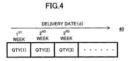
- FIG. 4 shows the structure of an actual order table 40 in which actual order quantities (quantities in firm orders) are indicated for each time bucket.
- the delivery date in this example, the delivery week
- the actual order quantity for each time bucket can be represented by QTY(d).
- the actual order quantity of the third week would be written QTY(3).
- FIG. 5 is a flow chart showing an order forecast method that is a preferred embodiment of the present invention.
- the order forecast in accordance with this embodiment starts with creation of the aforesaid forecast transition table 20 (30) and actual order table 40 (Step 1).
- the forecast transition table 20 (30) is created by arranging the received forecast information 10 in order of time so that the scheduled delivery dates (or scheduled delivery periods) are aligned.
- a forecast conversion coefficient table is created from the forecast transition table 20 (30) and actual order table 40 (Step S2).
- Each forecast conversion coefficient (hereinafter called simply “conversion coefficient") is defined as the ratio (QTY/F) of required quantity data contained in the forecast transition table 20 (30) to the corresponding actual order quantity contained in the actual order table 40.
- the forecast conversion coefficient table shows the conversion coefficients for the respective forecast receive dates arranged by forecast LT.
- the conversion coefficient is a value indicating how much the required quantity data differs from the actual order quantity. The more the value rises above 100%, the smaller is the required quantity data relative to the actual order quantity, and the more the value goes below 100% the larger is the required quantity data relative to the actual order quantity.
- FIG. 6 shows an example of a forecast conversion coefficient table.
- the forecast conversion coefficient table 50 contains a conversion coefficient for each combination of forecast LT and forecast receive date (in this example, week received).
- the conversion coefficients are derived from the data contained in the forecast transition table 20 of FIG. 2 and the actual order table 40.
- the columns of the forecast conversion coefficient table 50 represent forecast LT.
- the rows of the forecast conversion coefficient table 50 represent forecast receive date.
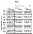
- FIG. 7 shows another example of a forecast conversion coefficient table.
- FIG. 8 shows still another example of a forecast conversion coefficient table.
- the forecast conversion coefficient table 70 of FIG. 8 is derived from the data of the forecast transition table 30 and actual order table 40.
- the cells constituting the forecast conversion coefficient table 70 are each assigned the ratio of the sum of four sets of required quantity data whose forecast LTs are consecutive to the sum of the corresponding actual order quantities.
- the foregoing forecast conversion coefficient tables are merely examples.
- the ratio (conversion coefficient) of the required quantity data to the actual order quantity is calculated for every forecast LT; in the forecast conversion coefficient table 60 of FIG. 7, it is calculated for two forecast LTs in combination; and in the forecast conversion coefficient table 70 of FIG. 8, it is calculated for four consecutive forecast LTs.
- the actual value is set in light of the type of customer (or customer group) and type of product (or product group).
- the forecast conversion coefficient table is used to calculate the standard deviation of the conversion coefficient for each forecast LT or forecast LT group (Step S3). Since, as explained above, the conversion coefficients are calculated for every forecast receive date, a large standard deviation of the conversion coefficients means that the variation among the conversion coefficients of the individual information receive dates is large, while a small standard deviation of the conversion coefficients means that the variation among the conversion coefficients of the individual forecast receive dates is small.
- Step S3 When the standard deviations of the conversion coefficients are calculated in Step S3, it is not necessary to use all of the conversion coefficients contained in each forecast LT or set of forecasts LTs.
- the number of conversion coefficients is large, i.e., when the forecast information 10 has been compiled over a long period, it is preferable to use only some of the conversion coefficients, including ones that correspond to recent forecast receive dates. This is because when there are very many conversion coefficients and all of them are used, the resulting inclusion of conversion coefficients corresponding to old forecast information and old actual order quantities degrades sensitivity to variation in the correlation between the forecast information and actual order quantities.
- the number of conversion coefficients used to calculate a standard deviation is not particularly defined and it is preferable instead to specify the number in accordance with the age of the forecast receive dates.
- An example would be to use only conversion coefficients obtained from forecast information with receive dates not more than, say, three months old.
- Step S4 the conversion coefficient standard deviations obtained in Step S3 whether or not they are equal to or less than a predetermined threshold is checked for each forecast LT or set of forecast LTs. This is for checking whether the variance of the conversion coefficients of the forecast receive dates is within an allowable range.
- the standard deviation exceeds the threshold, no definite correlation can be seen between the forecast information and actual order quantity. In such a case, therefore, it is judged that order forecast is impossible.
- the standard deviation is equal to or less than the threshold, it can be concluded that a definite correlation exists between the forecast information and actual order quantity. In such a case, therefore, the procedure is continued (goes to the next step explained later) on the judgment that order forecast is possible.
- the value of the threshold is not particularly limited, it is preferably set to be between 10% and less than 30%, more preferably set to be about 20%.
- the threshold is set below 10%, order forecast can be conducted only when the correlation between forecast information and actual order quantity is very strong, so that even cases in which order forecast should be possible are liable to be treated as ones in which forecast is impossible.
- the threshold is set at or higher than 30%, even cases in which the correlation between forecast information and actual order quantity is weak (or substantially nonexistent) come to be treated as subjects of order forecast, so that the forecast results become very inaccurate.
- the threshold is set to around 20%, highly accurate order forecast can be conducted with respect to most cases.
- the standard deviations and the predetermined threshold are compared for each forecast LT or each set of forecast LTs, it may happen that the standard deviations exceeds the threshold only for some of the forecast LTs or some of the sets of forecast LTs. In such a case, it is possible to advance to the next step on the understanding that order forecast is possible only with regard to the forecast LTs or sets of forecast LTs for which the standard deviations was equal to or less than the threshold. Alternatively, in order to conduct highly accurate order forecast, it is possible to decide that order forecast is impossible unless the standard deviations was found to be equal to or less than the threshold for all forecast LTs or all sets of forecast LTs.
- Step S5 the average value of the conversion coefficients is calculated for each forecast LT or set of forecast LTs (Step S5). If the calculation of the conversion coefficient standard deviations in Step S3 was done using not all but only some of the conversion coefficients, it is preferable here to calculate the average for only the conversion coefficients that were used to calculate the standard deviations. In the case where the conversion coefficient standard deviations exceeds the threshold only for some of the forecast LTs or some of the sets of forecast LTs, it is possible to calculate the average value of the conversion coefficients only with regard to the forecast LTs or sets of forecast LTs for which the standard deviations was equal to or less than the threshold.
- Step S6 the average value table 110 (120, 130) created in step S4 and the latest forecast information 10 are used to conduct an actual forecast order quantity calculation (Step S6).
- the forecast order quantity calculation in Step S6 is carried out by multiplying a scheduled quantity of orders contained in the latest forecast information 10 by the corresponding average value.
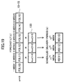
- FIG. 15 is a diagram for explaining a method of using the average value table 110 shown in FIG. 12 to calculate forecast order quantities from latest forecast information 10-6.
- the forecast order quantity calculation using the average value table 110 is done by respectively multiplying the required quantity data (F(6,7), F(6,8), F(6,9) and F(6,10)) contained in the latest forecast information 10-6 by the average values (Ave(1) to Ave(4)) of the average value table 110 having the same forecast LTs.
- These forecast order quantities are values that take into account the correlation between forecast information and actual order quantities for the products (product group) concerned of the customer (or customer group) concerned. The probability of their being closer to the actual quantity of firm orders than the required quantity data contained in the forecast information 10-6 is therefore very high. As a result, the risks of speculative production (delivery period risk owing to stockout and risk of stagnant inventory) can be reduced.
- FIG. 16 is a diagram for explaining a preferred method of using the average value table 120 shown in FIG. 13 to calculate forecast order quantities from latest forecast information 10-6.
- the latest forecast information 10-6 is the forecast information received next after the forecast information 10-5.
- the forecast order quantity calculation using the average value table 120 is done by respectively multiplying the required quantity data (F(6,7), F(6,8), F(6,9) and F(6,10)) contained in the latest forecast information 10-6 by the average values (Ave(1-2), Ave(2-3) and Ave(3-4)) of the average value table 120 having the same initial forecast LTs.
- the values of the required quantity data F(6,8) and F(6,9) whose initial forecast LTs are 2 weeks and 3 weeks are corrected by multiplying them by the corresponding average values Ave(2-3) and Ave(3-4) to obtain forecast order quantities RD(8) and RD(9)
- a forecast order quantity RD(10) corresponding to the required quantity data F(6, 10) cannot be obtained because the average value table 120 does not contain an average value whose initial forecast LT is 4 weeks.
- the correction of the required quantity data involves elements related to forecast LTs that are longer than the forecast LT concerned.
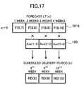
- FIG. 17 is a diagram for explaining another method of using the average value table 120 shown in FIG. 13 to calculate forecast order quantities from latest forecast information 10-6.
- the correction of the required quantity data involves elements related to forecast LTs that are shorter than the forecast LT concerned.
- order forecast is preferably done using the method shown in FIG. 16.
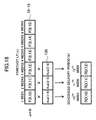
- FIG. 18 is a diagram for explaining a preferred method of using the average value table 130 shown in FIG. 14 to calculate forecast order quantities from latest forecast information 10-15.
- the latest forecast information 10-15 is the forecast information received next after the forecast information 10-14 shown in FIG. 3.
- the forecast order quantity calculation using the average value table 130 is done by a calculation method similar to that shown in FIG. 16, by respectively multiplying the required quantity data (F(9,10), F(9,11), F(9,12), F(9,13), F(9,14) and F(9,15)) contained in the latest forecast information 10-15 by the average values (Ave(1-4), Ave(2-5) and Ave(3-6)) of the average value table 130 having the same initial forecast LTs.
- forecast order quantities RD(13), RD(14) and RD(15) corresponding to the required quantity data F(9,13), F(9,14) and F(9,15) cannot be obtained because the average value table 130 does not contain average values whose initial forecast LTs are 4 weeks or longer.
- FIG. 19 is a diagram for explaining another method of using the average value table 130 shown in FIG. 14 to calculate forecast order quantities from latest forecast information 10-15.
- the correction of the required quantity data involves elements related to forecast LTs that are longer than the forecast LT concerned and elements related to forecast LTs that are shorter than the forecast LT concerned.
- order forecast is preferably done using the method shown in FIG. 18.
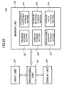
- FIG. 20 is a block diagram showing the structure of an order forecast system 200 according to a preferred embodiment of the present invention.
- the order forecast system 200 of this embodiment comprises a processing unit 210 for controlling the overall operation of the order forecast system 200, a memory unit 220 for storing data and the like to be explained later, an input unit 230 for inputting data required for order forecast, an a display unit 240 for displaying order forecast results.
- the memory unit 220 is equipped with a program storage section 221 for storing an order forecast program, a forecast storage section 222 for storing a forecast transition table (20, 30), an actual order quantity storage section 223 for storing an actual order table (40), a conversion coefficient storage section 224 for storing a forecast conversion coefficient table (50, 60, 70), a standard deviation storage section 225 for storing a standard deviation table (80, 90, 100), and an average value storage section 226 for storing an average value table (110, 120, 130).
- the sections 221 to 226 are not required to be independent physical devices but can be constituted by allotting to each an area of the recording region(s) of one or more recording devices (hard disk drives, semiconductor memories or the like). The assigned area may change dynamically.
- the order forecast program stored in the program storage section 221 is for operating the processing unit 210 to execute the procedure shown in FIG. 5.
- the processing unit 210 executes the procedures shown in FIG. 5 in accordance with the order forecast program stored in the program storage section 221. These procedures were set out in the earlier description and will not be explained again here.
- the forecast order quantities obtained as a result of the processing are displayed on the display unit 240, whereby the operator can check forecast order quantity for each scheduled delivery date (or scheduled delivery period).
- EDI Electronic Data Interchange
- the foregoing embodiments are configured to utilize forecast information and corresponding actual order quantity data received in the past to analyze the correlation between the forecast information and quantity of orders for each customer (or customer group) and each product (product group) and to utilize the result of the analysis to make order forecasts.
- the probability of the obtained numerical values being close to the actual quantities of firm orders is therefore very high.
- the fact that the order forecasts can be made with high accuracy works in turn to reduce the risks of speculative production (risk of not being able to meet delivery date because of stockout and risk of stagnant inventory).
- the feasibility of conducting an order forecast is decided based on whether or not the standard deviation is equal to or less than a predetermined threshold (see Step S4 in FIG. 5).
- the invention is not limited to this method. For example, it is possible to use the ratio of the standard deviation to the average value of the corresponding conversion coefficient (s/Ave) as a parameter and decide that order forecast is impossible when the parameter exceeds a threshold. When this criterion is adopted, the risk is further reduced when speculative production is carried out based on the finally obtained forecast order quantity.
- a decision is first made as to whether or not the standard deviations are equal to or less than a threshold (Step S4) and the calculation of the average value is conducted thereafter (Step S5).
- the calculation of the average value can instead be made before the decision.
- a conversion coefficient whose value differs greatly from the others (which has an abnormal value) can be eliminated from the calculation.
- Abnormality can be judged with reference to the standard deviation of the conversion coefficients. For instance, if the difference with respect to the average value obtained when the conversion coefficient considered abnormal is included is twice or more the standard deviation of the conversion coefficients, the conversion coefficient concerned can be treated as abnormal.
- the correlation between forecast information and actual quantity of orders is analyzed for each customer (or customer group) and each product (product group), and the result of the analysis is used to calculate a forecast order quantity. Since the order forecast can therefore be conducted with high accuracy, the risk of the supplier in speculative production can be reduced.
- FIG. 1 shows the data structure of ordinary forecast information.
- FIG. 2 shows an example of a forecast transition table.
- FIG. 3 shows another example of a forecast transition table.
- FIG. 4 shows the structure of an actual order table.
- FIG. 5 is a flow chart showing an order forecast method that is a preferred embodiment of the present invention.
- FIG. 6 shows an example of a forecast conversion coefficient table.
- FIG. 7 shows another example of a forecast conversion coefficient table.
- FIG. 8 shows still another example of a forecast conversion coefficient table.
- FIG. 9 shows an example of a standard deviation table.
- FIG. 10 FIG.
- FIG. 10 shows another example of a standard deviation table.
- FIG. 11 shows still another example of a standard deviation table.
- FIG. 12 shows an example of an average value table.
- FIG. 13 shows another example of an average value table.
- FIG. 14 shows still another example of an average value table.
- FIG. 15 is a diagram for explaining a method of using the average value table shown in FIG. 12 to calculate forecast order quantities from latest forecast information.
- FIG. 16 is a diagram for explaining a method of using the average value table shown in FIG. 13 to calculate forecast order quantities from latest forecast information.
- FIG. 17 is a diagram for explaining another method of using the average value table shown in FIG.
- FIG. 18 is a diagram for explaining a method of using the average value table shown in FIG. 14 to calculate forecast order quantities from latest forecast information.
- FIG. 19 is a diagram for explaining another method of using the average value table shown in FIG. 14 to calculate forecast order quantities from latest forecast information.
- FIG. 20 is a block diagram showing the structure of an order forecast system according to a preferred embodiment of the present invention.
- FIG. 21 shows an example of the time relationship between order receipt and production.
- FIG. 22 shows another example of the time relationship between order receipt and production.
- FIG. 23 shows still another example of the time relationship between order receipt and production.
Landscapes
- Business, Economics & Management (AREA)
- Engineering & Computer Science (AREA)
- Strategic Management (AREA)
- Economics (AREA)
- Development Economics (AREA)
- Entrepreneurship & Innovation (AREA)
- Accounting & Taxation (AREA)
- Finance (AREA)
- Marketing (AREA)
- Human Resources & Organizations (AREA)
- Theoretical Computer Science (AREA)
- Physics & Mathematics (AREA)
- General Business, Economics & Management (AREA)
- General Physics & Mathematics (AREA)
- Game Theory and Decision Science (AREA)
- Operations Research (AREA)
- Quality & Reliability (AREA)
- Tourism & Hospitality (AREA)
- Data Mining & Analysis (AREA)
- Educational Administration (AREA)
- Management, Administration, Business Operations System, And Electronic Commerce (AREA)
- Telephonic Communication Services (AREA)
Applications Claiming Priority (3)
| Application Number | Priority Date | Filing Date | Title |
|---|---|---|---|
| JP2003186648 | 2003-06-30 | ||
| JP2003186648A JP3954538B2 (ja) | 2003-06-30 | 2003-06-30 | 受注予測システム |
| PCT/JP2004/008195 WO2005001730A1 (fr) | 2003-06-30 | 2004-06-11 | Systeme, procede et programme de prediction de reception de commande |
Publications (2)
| Publication Number | Publication Date |
|---|---|
| EP1544779A1 true EP1544779A1 (fr) | 2005-06-22 |
| EP1544779A4 EP1544779A4 (fr) | 2006-11-08 |
Family
ID=33549698
Family Applications (1)
| Application Number | Title | Priority Date | Filing Date |
|---|---|---|---|
| EP04745789A Withdrawn EP1544779A4 (fr) | 2003-06-30 | 2004-06-11 | Systeme, procede et programme de prediction de reception de commande |
Country Status (7)
| Country | Link |
|---|---|
| US (1) | US20050288988A1 (fr) |
| EP (1) | EP1544779A4 (fr) |
| JP (1) | JP3954538B2 (fr) |
| CN (1) | CN1813264A (fr) |
| MY (1) | MY140254A (fr) |
| TW (1) | TW200511075A (fr) |
| WO (1) | WO2005001730A1 (fr) |
Families Citing this family (11)
| Publication number | Priority date | Publication date | Assignee | Title |
|---|---|---|---|---|
| US9117223B1 (en) * | 2005-12-28 | 2015-08-25 | Deem, Inc. | Method and system for resource planning for service provider |
| US8566219B2 (en) * | 2009-03-24 | 2013-10-22 | Trading Technologeis International, Inc. | System and method for a risk check |
| US10552849B2 (en) | 2009-04-30 | 2020-02-04 | Deem, Inc. | System and method for offering, tracking and promoting loyalty rewards |
| CN105469231A (zh) * | 2014-09-30 | 2016-04-06 | 三菱电机株式会社 | 订单数决定方法以及订单数决定装置 |
| JP6509063B2 (ja) * | 2014-09-30 | 2019-05-08 | 三菱電機株式会社 | 注文数決定方法、注文数決定装置及び注文数決定プログラム |
| CN107506842B (zh) * | 2017-06-29 | 2021-01-05 | 广州兴森快捷电路科技有限公司 | Pcb订单加投率预测方法和装置 |
| CN110837907B (zh) * | 2018-08-17 | 2024-06-18 | 北京京东乾石科技有限公司 | 一种预测波次订单量的方法和装置 |
| JP2021043671A (ja) * | 2019-09-10 | 2021-03-18 | 東芝テック株式会社 | 注文照会装置および情報処理システム |
| JP2021043673A (ja) * | 2019-09-10 | 2021-03-18 | 東芝テック株式会社 | 発注予測装置および情報処理システム |
| CN111199340B (zh) * | 2019-12-19 | 2023-07-11 | 上海东普信息科技有限公司 | 一种基于一联单的条码分配方法及系统 |
| CN117436709B (zh) * | 2023-12-20 | 2024-03-19 | 四川宽窄智慧物流有限责任公司 | 一种跨区域订单数据统筹预警方法 |
Family Cites Families (7)
| Publication number | Priority date | Publication date | Assignee | Title |
|---|---|---|---|---|
| US6401070B1 (en) * | 1996-10-11 | 2002-06-04 | Freddie Mac | System and method for providing house price forecasts based on repeat sales model |
| US5963919A (en) * | 1996-12-23 | 1999-10-05 | Northern Telecom Limited | Inventory management strategy evaluation system and method |
| US6205431B1 (en) * | 1998-10-29 | 2001-03-20 | Smart Software, Inc. | System and method for forecasting intermittent demand |
| JP2001325488A (ja) * | 2000-05-16 | 2001-11-22 | Hitachi Ltd | 需要情報取得方法および需要情報取得システム |
| JP2002012308A (ja) * | 2000-06-30 | 2002-01-15 | Hitachi Ltd | 在庫管理方法 |
| JP2002073752A (ja) * | 2000-09-04 | 2002-03-12 | Kao Corp | 受注予測システムおよび受注管理システムならびに生産管理システム |
| JP2002318613A (ja) * | 2001-04-20 | 2002-10-31 | Rubycon Corp | 部品供給管理システム |
-
2003
- 2003-06-30 JP JP2003186648A patent/JP3954538B2/ja not_active Expired - Fee Related
-
2004
- 2004-06-11 US US10/532,984 patent/US20050288988A1/en not_active Abandoned
- 2004-06-11 WO PCT/JP2004/008195 patent/WO2005001730A1/fr not_active Ceased
- 2004-06-11 CN CNA2004800184955A patent/CN1813264A/zh active Pending
- 2004-06-11 EP EP04745789A patent/EP1544779A4/fr not_active Withdrawn
- 2004-06-28 MY MYPI20042549A patent/MY140254A/en unknown
- 2004-06-30 TW TW093119470A patent/TW200511075A/zh unknown
Non-Patent Citations (2)
| Title |
|---|
| No Search * |
| See also references of WO2005001730A1 * |
Also Published As
| Publication number | Publication date |
|---|---|
| CN1813264A (zh) | 2006-08-02 |
| US20050288988A1 (en) | 2005-12-29 |
| JP2005025245A (ja) | 2005-01-27 |
| WO2005001730A1 (fr) | 2005-01-06 |
| EP1544779A4 (fr) | 2006-11-08 |
| JP3954538B2 (ja) | 2007-08-08 |
| TW200511075A (en) | 2005-03-16 |
| MY140254A (en) | 2009-12-31 |
Similar Documents
| Publication | Publication Date | Title |
|---|---|---|
| EP1640897A1 (fr) | Systeme de prediction de reception d'ordre, procede de prediction de reception d'ordre et programme de prediction de reception d'ordre | |
| US6453303B1 (en) | Automated analysis for financial assets | |
| US7822692B2 (en) | Automated control of pricing using markdown profiles | |
| US20050222888A1 (en) | Method of creating production plan of demand variation input type and method of creating production plan minimizing risk of demand variations | |
| Sahin et al. | Quality, warranty and preventive maintenance | |
| US8359116B2 (en) | Production management system | |
| EP1544779A1 (fr) | Systeme, procede et programme de prediction de reception de commande | |
| US20060036470A1 (en) | Systems and methods for providing a pharmacy management analysis report | |
| KR20030043678A (ko) | 매상 예측 장치 및 매상 예측 방법 | |
| Arana et al. | Service level of pharmaceutical supply chain applying optimal policy: Case study in Lima, Peru | |
| Shurrab et al. | Untangling the complexity generating material delivery “schedule instability”: insights from automotive OEMs | |
| Jeang | Economic production order quantity and quality | |
| JP4812269B2 (ja) | 需要変動リスク最小生産計画生成方法 | |
| JP2020119029A (ja) | 発注情報計算プログラム、装置、及び方法 | |
| US7613626B1 (en) | Integrated price management systems with future-pricing and methods therefor | |
| CN118071248A (zh) | 一种物料产供销的异常追溯方法以及追溯装置 | |
| US20050131755A1 (en) | Sales rolling forecast managing system and method and recording medium | |
| US20260099815A1 (en) | Method and system for managing part inventory between related facilities | |
| JP2001312542A (ja) | 在庫量決定装置及び在庫量決定方法 | |
| US20050097065A1 (en) | System and method for analyzing relationships between sourcing variables | |
| Li et al. | Determining the optimal procurement policy and maximum allowable lifespan for machining tools with stochastically distributed toollife | |
| Kumar et al. | Medical inventory cost reduction: A survey based study | |
| US20260099812A1 (en) | Determination of a part inventory safety factor | |
| Islan de Castro Mechanical | Inventory management optimization for capital goods maintenance | |
| Ploszczuk et al. | How Postponement Strategy Can Reduce Cost and Lead Time for Pharma Supply Chains |
Legal Events
| Date | Code | Title | Description |
|---|---|---|---|
| PUAI | Public reference made under article 153(3) epc to a published international application that has entered the european phase |
Free format text: ORIGINAL CODE: 0009012 |
|
| AK | Designated contracting states |
Kind code of ref document: A1 Designated state(s): AT BE BG CH CY CZ DE DK EE ES FI FR GB GR HU IE IT LI LU MC NL PL PT RO SE SI SK TR |
|
| AX | Request for extension of the european patent |
Extension state: AL HR LT LV MK |
|
| 17P | Request for examination filed |
Effective date: 20050831 |
|
| DAX | Request for extension of the european patent (deleted) | ||
| A4 | Supplementary search report drawn up and despatched |
Effective date: 20061011 |
|
| 17Q | First examination report despatched |
Effective date: 20071122 |
|
| STAA | Information on the status of an ep patent application or granted ep patent |
Free format text: STATUS: THE APPLICATION IS DEEMED TO BE WITHDRAWN |
|
| 18D | Application deemed to be withdrawn |
Effective date: 20080403 |