WO2014002319A1 - 最適指標生成装置、最適指標生成方法、最適指標生成プログラム及び最適指標生成サーバ - Google Patents
最適指標生成装置、最適指標生成方法、最適指標生成プログラム及び最適指標生成サーバ Download PDFInfo
- Publication number
- WO2014002319A1 WO2014002319A1 PCT/JP2012/084031 JP2012084031W WO2014002319A1 WO 2014002319 A1 WO2014002319 A1 WO 2014002319A1 JP 2012084031 W JP2012084031 W JP 2012084031W WO 2014002319 A1 WO2014002319 A1 WO 2014002319A1
- Authority
- WO
- WIPO (PCT)
- Prior art keywords
- time
- information
- index
- devices
- management system
- Prior art date
- Legal status (The legal status is an assumption and is not a legal conclusion. Google has not performed a legal analysis and makes no representation as to the accuracy of the status listed.)
- Ceased
Links
Images
































Classifications
-
- G—PHYSICS
- G06—COMPUTING OR CALCULATING; COUNTING
- G06Q—INFORMATION AND COMMUNICATION TECHNOLOGY [ICT] SPECIALLY ADAPTED FOR ADMINISTRATIVE, COMMERCIAL, FINANCIAL, MANAGERIAL OR SUPERVISORY PURPOSES; SYSTEMS OR METHODS SPECIALLY ADAPTED FOR ADMINISTRATIVE, COMMERCIAL, FINANCIAL, MANAGERIAL OR SUPERVISORY PURPOSES, NOT OTHERWISE PROVIDED FOR
- G06Q10/00—Administration; Management
-
- G—PHYSICS
- G06—COMPUTING OR CALCULATING; COUNTING
- G06Q—INFORMATION AND COMMUNICATION TECHNOLOGY [ICT] SPECIALLY ADAPTED FOR ADMINISTRATIVE, COMMERCIAL, FINANCIAL, MANAGERIAL OR SUPERVISORY PURPOSES; SYSTEMS OR METHODS SPECIALLY ADAPTED FOR ADMINISTRATIVE, COMMERCIAL, FINANCIAL, MANAGERIAL OR SUPERVISORY PURPOSES, NOT OTHERWISE PROVIDED FOR
- G06Q50/00—Information and communication technology [ICT] specially adapted for implementation of business processes of specific business sectors, e.g. utilities or tourism
- G06Q50/04—Manufacturing
-
- Y—GENERAL TAGGING OF NEW TECHNOLOGICAL DEVELOPMENTS; GENERAL TAGGING OF CROSS-SECTIONAL TECHNOLOGIES SPANNING OVER SEVERAL SECTIONS OF THE IPC; TECHNICAL SUBJECTS COVERED BY FORMER USPC CROSS-REFERENCE ART COLLECTIONS [XRACs] AND DIGESTS
- Y02—TECHNOLOGIES OR APPLICATIONS FOR MITIGATION OR ADAPTATION AGAINST CLIMATE CHANGE
- Y02P—CLIMATE CHANGE MITIGATION TECHNOLOGIES IN THE PRODUCTION OR PROCESSING OF GOODS
- Y02P90/00—Enabling technologies with a potential contribution to greenhouse gas [GHG] emissions mitigation
- Y02P90/30—Computing systems specially adapted for manufacturing
-
- Y—GENERAL TAGGING OF NEW TECHNOLOGICAL DEVELOPMENTS; GENERAL TAGGING OF CROSS-SECTIONAL TECHNOLOGIES SPANNING OVER SEVERAL SECTIONS OF THE IPC; TECHNICAL SUBJECTS COVERED BY FORMER USPC CROSS-REFERENCE ART COLLECTIONS [XRACs] AND DIGESTS
- Y02—TECHNOLOGIES OR APPLICATIONS FOR MITIGATION OR ADAPTATION AGAINST CLIMATE CHANGE
- Y02P—CLIMATE CHANGE MITIGATION TECHNOLOGIES IN THE PRODUCTION OR PROCESSING OF GOODS
- Y02P90/00—Enabling technologies with a potential contribution to greenhouse gas [GHG] emissions mitigation
- Y02P90/80—Management or planning
Definitions
- the present invention relates to an optimum index generation device for supplying index information on a plurality of devices to a production management system that controls a plurality of devices to produce various kinds of products.
- Q-time constraint cracking is a loss of quality / value and waste of cost, time, resources, energy, etc. Brought to a great loss.
- the unit price of a large-diameter, highly-integrated product wafer in recent years is as high as 1 million yen to several 10 million yen.
- the cost of production facilities is also high, from several tens of millions of yen to several billions of yen, and the depreciation cost accounts for more than 50% of the annual production cost, so it is extremely important to secure good production volume per unit time. It is an important issue.
- the occurrence of rework causes an increase in processing process load, leading to an increase in secondary rework.
- the present situation is that the optimal production management method (especially production scheduling method) for achieving other production targets while complying with Q-time constraints has not been established yet. is there.
- the reasons for staying in such a current situation are mainly due to the following three problems.
- the first problem is that in order to comply with Q-time constraints, it is necessary to limit the production flow rate, which is a contradictory requirement to the achievement of other production goals (eg, throughput improvement). Therefore, it is difficult to optimize multipurpose production of multiple varieties.
- analytical modeling is difficult because the processing unit of the manufacturing process is batch and the processing unit changes, or a multitask type in which a plurality of different processes are internally performed.
- the second problem is that the preventive maintenance of manufacturing equipment, which is the main cause of Q-time constraint cracking, has not been optimized.
- the number of operating units decreases, and the production capacity of the process (device group) is significantly reduced.
- the logistics of the subsequent process will be greatly changed.
- the Q-time constraint is likely to be broken, which adversely affects other production targets.
- the plan for preventive maintenance aims at minimizing the costs related to preventive maintenance, and does not take Q-time constraints into consideration [Non-Patent Document 2 etc.].
- the third problem is that the simultaneous management of the whole is essential, as dozens of Q-time constraints intersperse and interfere with each other in the manufacturing flow.
- a high-speed calculation method is required to manage the entire manufacturing flow of hundreds of steps in real time.
- the Q-time constraints include, for example, 60 or more Q-time constraints on a memory manufacturing flow of about 700 steps.
- mutual interference it is necessary to simultaneously manage one Q-time constraint, but the other Q-time constraint can not be observed.
- a problem common to the prior art is to realize a calculation time adaptable to real time management.
- the calculation order of the mixed integer programming applied in Non-Patent Document 1 and Non-Patent Document 2 is index time, so that it is limited to the production schedule for a production period of about one week for a part of production process. Without it, it can not be calculated within a realistic time.
- the production period is as long as 1.5 months to 2.5 months, and the number of processes included in the production process is high speed for optimum management of a large scale production system with about 300 to 1000 processes. Calculation method is required.
- Non-Patent Document 1 a method of managing the stay time of each lot
- Patent Document 2 a method of managing the stay time by the number of lots
- Patent Document 1 a production management system limited to Q-time constraints after completion of the previous process and before construction for the purpose of complying with Q-time constraint values and achieving the target production volume for semiconductor pretreatment plants.
- process processing time the number of processes, and the number of apparatuses, calculation of a plurality of improvement plan candidates and determination of their feasibility are performed, and if there is even one improvement plan that can be implemented, improvement is made, and improvement is not made.
- the workpiece information from the processing device is linked to the host computer of the conventional transfer system, the appropriate reference inventory is calculated, and the computer automatically instructs the transfer to automatically guarantee the work quality guarantee time. maintain.
- the automatic management system can solve the quality assurance time of workpieces and overtime of Q-time, and can maintain the quality assurance time.
- the automated management system provided has been reported.
- Non-Patent Document 1 reports the results of joint research between National Taiwan University, University of Connecticut and Inotera Memories.
- two Q-time constraints continue from the end of the first step to the start of the process of the second step and from the end of the process of the second step to the start of the process of the third step It targets a single Q-time constraint interval.
- Heuristics to be compared is an empirical method that starts the processing of the second step when the remaining processing time of the third step reaches 60 minutes.
- Non-Patent Document 2 results of joint research with US universities, companies, and members of ISMI are reported.
- the PM schedule is calculated as a result of adjusting an externally provided base schedule using a mixed integer programming problem aiming to minimize the cost of the PM task.
- the simulation results of four cases using actual industrial data and factory model are shown, and the results show that the enhancement of PM work and the equipment productivity have been improved well. It also provides templates and guidelines for other implementations of the PM optimization algorithm used in PMOST.
- Patent Document 1 has a problem that Q-time constraint cracking can not be prevented because modeling accuracy is low.
- the emphasis was put on the management system (information system), such as conveyance, and it was a technique which lacks practicability in the viewpoint of improvement of production efficiency.
- Non-Patent Document 1 Although the Q-time constraint is prone to breakage, optimization is directed without handling the lower limit of the Q-time constraint, the combination becomes enormous when dealing with a large number of Q-time constraints, There is a problem that high-speed calculations that can be used in real time can not be expected.
- Non-Patent Document 1 deals with only one typical type of Q-time constraint section. Moreover, although patent document 1 takes four types of structures as a subject, only one type of structure is providing the management method. As a result, neither prior art provides a way to comprehensively define and totally control the structure of all Q-time constraints.
- the present invention has been made in view of the above circumstances, and Q-time constraints can be reliably observed even in situations where Q-time constraints that are not achieved by the conventional method are likely to occur, and the non-defective product throughput is improved. And provide optimal operation management conditions that can achieve cost reduction and reduction of environmental impact, resource consumption and energy consumption.
- analysis methods and appropriateness are also applied to handling of multi-product production, preventive maintenance of equipment, mutual interference of multiple Q-time constraints, which are the main causes of Q-time constraint cracking. It aims to make it easy to simultaneously achieve improvement in non-defective product throughput and cost reduction and environmental load reduction while complying with Q-time constraints by providing a new management method.
- the invention according to claim 1 is optimum for supplying index information on a plurality of devices and products to a production management system which controls a plurality of devices to produce various kinds of products.
- An information generating unit for inputting information related to the plurality of devices and products via the production management system, and a limit value of staying time between processing steps by the plurality of devices based on the input information.
- An optimal index generating device for analyzing the Q-time structure showing the following, and an optimal theoretical value calculation unit for calculating the optimal number of Kanbans and buffer size for each type based on the input information and the Q-time structure ,
- An index calculation unit that outputs the calculated information as index information, and a size of a batch combination waiting time related to the arrival of the product and an upper limit value of the Q-time constraint
- an optimal load rule determination unit that calculates the boundary value of the arrival rate at which the agent switches and determines an appropriate load rule, and the production management system performs optimal index information and load rules calculated by the index calculation unit.
- the invention according to claim 3 is an optimum index generation method for supplying index information on the plurality of apparatuses and products to a production management system that controls a plurality of apparatuses to produce various types of products,
- An information input step of inputting information on a plurality of devices and products via the production management system, and analysis of a Q-time structure indicating a limit value of staying time between processing steps by the plurality of devices from the input information
- the index calculation step to be output as index information, and the size relation between the batch assembly waiting time related to the arrival of the product and the upper limit value of the Q-time constraint Calculating the boundary value of the arrival rate at which is switched, and performing an optimal load rule determination step to determine an appropriate load rule, and performing the optimal index information calculated by the index calculation step and the load rule in the production management system It is a method of generating an optimal index characterized by
- the invention according to claim 11 is an optimum index generation server for transmitting index information on a plurality of devices and products via a communication line to a production management system that controls a plurality of devices to produce various types of products.
- An information receiving unit for receiving information on the plurality of devices and products via the production management system, and a Q indicating a limit value of staying time between processing steps by the plurality of devices based on the received information
- a Q-time structure analysis unit for analyzing a -time structure, an optimal theoretical value calculation unit for calculating an optimum number of Kanbans and a buffer size for each type based on the received information and the Q-time structure, and
- the index calculation unit that outputs the calculated information as index information, and the magnitude relationship between the batch assembly waiting time related to the arrival of the product and the upper limit value of the Q-time constraint
- an optimal load rule determination unit that calculates the boundary value of the replacement arrival rate and determines an appropriate load rule, and the optimal index information calculated by the index calculation unit and the load rule are used in the production
- the invention according to claim 12 is performed by a server that transmits index information on the plurality of devices and products via a communication line to a production management system that controls the plurality of devices to produce various types of products.
- An optimal index generating method comprising: an information receiving step of receiving information on the plurality of devices and products via the production management system; and limiting a staying time between processing steps by the plurality of devices based on the received information.
- Q-time structure analysis step for analyzing the Q-time structure showing the value, and the optimal theoretical value calculation for calculating the optimum number of Kanbans and the buffer size according to the type based on the received information and the Q-time structure Step, index calculation step of outputting the calculated information as index information, batch set waiting time related to arrival of product, The optimal index calculated by the index calculation step, performing the optimal load rule determination step of calculating the boundary value of the arrival rate at which the magnitude relation with the upper limit value of the -time constraint switches, and determining the appropriate load rule. It is an optimal index generation method characterized by transmitting information and a load rule to said production control system.
- the invention according to claim 13 is an optimal index generation for supplying index information on a plurality of devices to a production management system for controlling a plurality of devices provided in a production execution system for producing a variety of products.
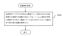
- An apparatus comprising: an information input unit for inputting, via the production management system, information on a plurality of apparatuses included in the production execution system; and a bottleneck in processing steps by the plurality of apparatuses based on the input information
- a bottleneck location analysis unit that analyzes the location and maximum flow rate, and a Q-time constraint structure analysis unit that analyzes the structure of Q-time constraint sections in which one or more Q-time constraints exist from the input information
- an index calculation unit for outputting as index information, an information input unit for inputting information related to a plurality of devices included in the production execution system via the production management system, and a commonly used device having the capability of using the plurality of devices regularly
- Device division calculation unit for dividing into a plurality of substitute devices having substitute capacity and optimum number of times of operation, operation timing and content of operation of the plurality of regular devices and substitute devices from the calculated device classification and input information
- a theoretical value calculation unit a time index calculation unit that calculates a preventive maintenance start time for the regular device and the alternative device, the bottleneck location, the maximum flow rate, the Q-time structure, and the device category and the time indicator
- an optimal theoretical value calculating unit that calculates the optimal number of Kanbans and the buffer size for each type, and the calculated optimal theoretical value as index information.
- An index calculation unit, and a procedure execution control unit simultaneously managing all Q-time constraints scattered throughout the manufacturing flow included in the production execution system, calculated by the time index calculation unit and the index calculation unit An optimal index generating device characterized in that the optimal index information is supplied to the production management system and the engineering operation system, and the optimal index information calculated by the time index calculation unit is supplied to the production management system. .
- the invention according to claim 14 is an optimum index generation for supplying index information on a plurality of devices to a production management system for controlling a plurality of devices provided in a production execution system for producing a variety of products.
- a method comprising: inputting information about a plurality of devices included in the production execution system via the production management system; and a bottleneck in processing steps by the plurality of devices based on the input information Bottleneck point analysis step for analyzing point and maximum flow rate, and Q-time constraint structure analysis step for analyzing the structure of Q-time constraint section in which one or more Q-time constraints exist from the input information And the optimal number of pieces of Kanban by variety based on the bottleneck location, the maximum flow rate and the Q-time structure, and An index calculation step of calculating buffer size and outputting as index information, an information input step of inputting information related to a plurality of devices included in the production execution system via the production management system, and a capability of using the plurality of devices in common use
- the invention according to claim 18 relates to a production management system for controlling a plurality of devices provided in a production execution system for producing a variety of products, index information on the plurality of devices via a communication line.
- An optimal index generation server for transmitting, an information receiving unit for receiving information on a plurality of devices included in the production execution system via the production management system, and a processing step by the plurality of devices based on the received information
- a bottleneck location analysis unit for analyzing the bottleneck location and the maximum flow rate in Q, and Q for analyzing the structure of the Q-time constraint interval in which one or more Q-time constraints exist from the received information
- the optimal number of Kanbans by type and
- An index calculation unit that calculates buffer size and outputs it as index information, an information reception unit that receives, via the production management system, information on a plurality of devices included in the production execution system,
- the device classification and calculation unit for dividing into a regular device having
- the optimal theoretical value calculation unit to calculate, the time index calculation unit to calculate the preventive maintenance start time for the regular device and the alternative device, the bottleneck location, the maximum flow rate, the Q-time structure and the device category and the time An optimum theoretical value calculating unit for calculating an optimum number of Kanbans by type and a buffer size based on the index, and the calculated optimum theoretical value.
- An index calculation unit for outputting as information, and the optimum index information calculated by the time index calculation unit and the index calculation unit is transmitted to the production management system or the engineering business system, and calculated by the time index calculation unit It is an optimum index generation server characterized by transmitting the optimum index information thus obtained to the production management system.
- the invention according to claim 19 relates to a production management system for controlling a plurality of devices provided in a production execution system for producing a variety of products, index information on the plurality of devices via a communication line.
- An optimal index generation method executed by a transmitting server comprising: an information receiving step of receiving information on a plurality of devices included in the production execution system via the production management system; and the plurality of information from the received information.
- the bottleneck location analysis step for analyzing the bottleneck location and the maximum flow rate in the processing process by the device, and the structure of the Q-time constraint interval in which one or more Q-time constraints exist from the received information Based on the Q-time constraint structure analysis step to analyze, the bottleneck location, the maximum flow rate and the Q-time structure,
- a device classification calculating step of dividing the plurality of devices into a regular device having a regular capability and an alternate device having an alternate capability, and operation of the plurality of regular devices and the alternate device from the computed device category and the received information
- the optimal theoretical value calculating step for calculating the number of times, the operation time, and the operating condition, and the time index calculating step for calculating the preventive maintenance start time for the regular device and the alternative device are executed, As well as
- the invention according to claim 20 is an optimum index generating device for supplying index information regarding the plurality of devices to a production management system that controls a plurality of devices for producing a variety of products,
- An information input unit for inputting information related to the device through the production management system, a device classification calculation unit for dividing the plurality of devices into a regular device having regular capability and an alternate device having alternative capability;
- Optimum theoretical value calculating unit for calculating the number of times of operation, operation time and operation conditions of the plurality of regular devices and alternative devices from the device classification and the input information; and prevention based on the calculation result about the regular devices and the alternative devices
- a start / end time calculation unit for calculating maintenance start / end time, and said production management system or the optimum start / end time information calculated by the start / end time calculation unit It is optimal indicator generation unit and supplying the engineering business system.
- the invention according to claim 22 is an optimum index generation method for supplying index information on the plurality of devices to a production management system that controls a plurality of devices for producing various types of products,
- the information input step of inputting information on the device of the device via the production management system, the device classification calculating step of dividing the plurality of devices into a regular device having regular capability and an alternate device having alternate capability;
- Optimum theoretical value calculating step of calculating the number of times of operation, operation time and operation condition of the plurality of regular devices and alternative devices from the device classification and the input information, and the prevention concerning the regular devices and the alternative devices from the calculation result Performing the start / end timing calculation step of calculating the maintenance start / end timing, and performing the optimum start / end calculated by the start / end timing calculation step It is optimal index generation method and supplying the period information to the production management system and engineering business system.
- the invention according to claim 25 is an optimum index generation server for transmitting index information on the plurality of devices via a communication line to a production management system that controls a plurality of devices for producing various types of products.
- An information input unit for receiving information on the plurality of devices via the production management system, and a device classification calculation unit for dividing the plurality of devices into a regular device having regular capability and an alternate device having alternate capability
- An optimal theoretical value calculation unit for calculating the number of times of operation, operation time and operation conditions of the plurality of regular devices and alternative devices from the calculated device category and the input information; and the regular devices from the calculation result
- a start / end timing calculation unit for calculating a preventive maintenance start / end timing concerning the alternative device, and said optimum start / end timing information calculated by said start / end timing calculation unit It is optimal indicator generation server and transmits the produced management systems and engineering services system.
- the invention according to claim 26 is the optimum executed by a server that transmits index information on a plurality of devices via a communication line to a production management system that controls a plurality of devices for producing various types of products.
- a method of generating an index comprising: an information receiving step of receiving information on the plurality of devices via the production management system; and dividing the plurality of devices into a regular device having regular capability and an alternate device having alternative capability.
- the optimal theoretical value calculating step of calculating the number of times of operation, operation time and operation condition of the plurality of regular devices and alternative devices from the calculated device category and the received information; Performing a start / end timing calculation step of calculating a preventive maintenance start / end timing concerning the regular use device and the alternative device, It is optimal index generation method and transmitting the optimal start and end time information calculated in the production management system and engineering business system by.
- the invention according to claim 27 is an optimal index generation for supplying index information on a plurality of devices to a production management system for controlling a plurality of devices provided in a production execution system for producing a variety of products.
- An apparatus comprising: an information input unit for inputting, via a production management system, information on a plurality of apparatuses included in the production execution system; and a restriction on stay time between processing steps by the plurality of apparatuses based on the input information Based on the Q-time structure analysis unit that analyzes the Q-time constraints that show the value, and the number and buffer size optimal for each type based on the input information and the Q-time structure, as index information
- An index calculation unit to output, and an information input unit to input information on a plurality of devices included in the production execution system from a production management system;
- Device classification calculation unit for dividing the plurality of devices into a regular device having a regular ability and an alternate device having an alternative ability, and operation of the plurality of regular devices and alternative devices from the calculated device category and the input information
- the invention according to claim 29 is an optimal index generation for supplying index information on a plurality of devices to a production management system for controlling a plurality of devices provided in a production execution system for producing a variety of products.
- a method comprising: inputting information about a plurality of devices included in the production execution system via a production management system; limiting a staying time between processing steps by the plurality of devices based on the input information Based on the Q-time structure analysis step of analyzing the Q-time constraint indicating the value and the number and buffer size optimal for each type based on the input information and the Q-time structure as index information
- Optimal theoretical value calculating step for calculating the number of times of operation, operating time and operating conditions of
- the invention according to claim 32 relates to a production management system for controlling a plurality of devices provided in a production execution system for producing a variety of products, index information on the plurality of devices via a communication line.
- An information receiving unit which is an optimum index generation server for transmitting information about a plurality of devices included in the production execution system via a production management system; and processing steps by the plurality of devices based on the received information
- Q-time structure analysis unit that analyzes Q-time constraints indicating the limit value of stay time, and based on the received information and the Q-time structure, calculate the optimal number and buffer size of varieties by type
- a device classification calculation unit for dividing the plurality of devices into a regular device having regular capability and an alternate device having alternate capability, and the plurality of regular devices from the calculated device category and the received information
- Optimal theoretical value calculation unit for calculating the number of times of operation, operation time and
- the invention according to claim 33 relates to a production management system for controlling a plurality of devices provided in a production execution system for producing a variety of products, with index information on the plurality of devices via a communication line.
- An optimal index generating method executed by a transmitting server comprising: an information receiving step of receiving information on a plurality of devices included in the production execution system via a production management system; and the plurality of devices from the received information.
- Q-time structure analysis step for analyzing the Q-time constraint indicating the limit value of stay time between processing steps, and the optimal number of varieties and the number of varieties based on the received information and the Q-time structure
- An index calculating step of calculating a buffer size and outputting it as index information, and a plurality of devices included in the production execution system Receiving an information receiving step of receiving information from a production management system, a device classification calculating step of dividing the plurality of devices into a regular device having a regular ability and an alternate device having an alternative ability, and the calculated device category Calculation step of calculating the number of times of operation, operation time and operation conditions of the plurality of regular devices and alternative devices from the stored information, and the start / end time calculating step of calculating preventive maintenance start time for the regular devices and alternative devices , And transmits the optimum start / end time information calculated by the start / end time calculation step to the production management system or the engineering business system, and the process capability determined by the calculated start / end time differs.
- analysis methods and appropriateness are also applied to handling of multi-product production, preventive maintenance of equipment, mutual interference of multiple Q-time constraints, which are the main causes of Q-time constraint cracking. It is possible to simultaneously achieve improvement in non-defective product throughput, cost reduction and environmental load reduction while complying with Q-time constraints by providing a new management method.
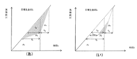
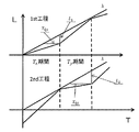
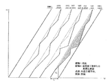
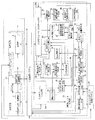
- FIG. 7 is a diagram showing a Q-time restricted section of the semiconductor pre-process as a specific example of the process shown in FIG. 1; It is a figure for demonstrating a performance evaluation index and its calculation method. It is a figure which shows the apparatus (washing
- FIG. 6 is a job allocation diagram in consideration of fixed maintenance. It is a figure for demonstrating [2] of conditions (3) of a JAMP method.
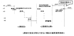
- FIG. 7 is a diagram for describing an apparatus operation guideline 1 in the case where complete decentralization can not be performed in one cycle.
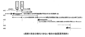
- FIG. 17 is a diagram for describing an apparatus operation guideline 2 in the case where complete decentralization can not be performed in one cycle. It is a figure for demonstrating perfect dispersion-ization (the 2nd period or subsequent one) of the pointer
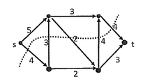
- FIG. 5 illustrates parallel network flows and minimum cuts.
- FIG. 5 illustrates parallel network flow. It is an explanatory view showing a production process model of nonpatent literature 1.
- Non-Patent Document 1 It is a figure which shows the system configuration
- FIG. 60 shows a method of (2) minimum setup cycle calculation of the stage change cycle calculation unit 53.
- 63 is a diagram showing an example of a method of determining the device classification and the maintenance order.
- FIG. 60 shows a method of using the set-up in the JAMP-wS optimum logical value calculation unit 55 (specified by the user at the auxiliary input unit 52).
- Performance comparison with a typical rule It is a figure which shows a setup rate and a non-defective item production rate (conventional method, this invention).
- Performance comparison with typical rules Overall installation efficiency (conventional method, the invention).
- FIG. 1 It is a figure which shows the system configuration
- FIG. 5 is a diagram showing production capacity distribution and production spikes in a parallel structure of production processes. It is a figure which shows Example 1 (arrival interlocking
- Example 2 stepwise fluctuation absorption dispersion
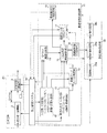
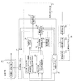
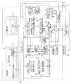
- the optimum index generating device 11 according to the first embodiment of the present invention is, for example, a process (apparatus group) 2 and a process (apparatus group) 3 which are respectively provided in production process # 1 for producing a semiconductor.
- a production management system 10 that manages a schedule is a target of control.
- the production management system 10 is a data input / output destination of the production physical distribution control method (hereinafter referred to as the CKB method), extracts various input data, delivers it to the input units 12 and 13 (CKB method), and calculates the CKB method Receive and create a schedule.
- the production management system 10 inputs various production management data and CKB theoretical value calculation results from the optimum index generation device 11, extracts data necessary for CKB method calculation, delivers it to the input unit 12 and 13, and CKB method theory The values are used to calculate the production flow schedule, including the Q-time constraint interval.
- the production management system 10 calculates an optimal schedule based on the CKB method theoretical value calculation result and a scheduling algorithm (dispatching rule, setup rule, etc.).
- the production management system 10 outputs information on the production schedule to each input unit 12, 13.
- the optimum index generation device 11 includes an input unit 12, an auxiliary input unit 13, a Q-time structure analysis unit 14, a CKB optimum logic value calculation unit 15, a sensitivity analysis unit (CKB characteristic) 16, and an index calculation.
- a unit 17 and a sensitivity analysis unit (performance characteristic) 18 are provided.
- the input unit 12 is information related to production planning, product information, process planning and the like via the production management system 10 and the production planning device, production timing and quantity of each type, production flow (by type), and an apparatus of each process Type and number, type-device correspondence table, processing time for each type, load size, load interval, minimum required time other than main processing (conveying time, setup time, etc.), Q-time restriction time (upper limit, lower limit) Enter).
- the auxiliary input unit 13 receives setup time (manufacturing conditions), delivery date (production conditions), equipment failure / maintenance plan / result data, equipment down time data (equipment management information) from the production management system 10, standby points of the equipment Enter the presence or absence of and the capacity of the waiting place (facility conditions) etc.
- the auxiliary input unit 13 inputs non-essential input data, but in practice, the CKB optimum logical value calculating unit 15 in the next step collectively performs preprocessing on important data to obtain average setup time (product types and devices -Outputs delivery time factor (product type and process), MTBF (average failure interval), MTTR (average repair time), presence / absence of waiting of the device, capacity value, etc.
- the CKB method optimal theoretical value calculation unit 15 performs more detailed calculation.
- the Q-time structure analysis unit 14 analyzes the structure of the Q-time constraint, detects the structure of the Q-time constraint section, performs conversion as necessary, and outputs Q-time constraint section process information.
- the analysis result can be recorded in the internal storage unit 14a and used as master data of the Q-time restricted section.
- the internal storage unit 14a is updated.
- the CKB optimum logical value calculation unit 15 inputs all the data from the input unit 12, the data from the auxiliary input unit 13, and the data from the Q-time structure analysis unit.
- the optimum number of Kanbans is calculated, the optimum buffer size is calculated, and the optimum number of Kanbans and the optimum buffer size are output.
- the information in the internal storage 16 a of the sensitivity analysis unit (CKB characteristic) 16 faster calculation becomes possible.
- the sensitivity analysis unit (CKB characteristic) 16 inputs Q-time section process information, traffic intensity (variable), lot arrival rate (sort by type) (variable), process capacity (variable), load size (variable), etc. , Calculate the change characteristics of CKB theoretical value calculation results when the lot arrival rate or the processing capacity of the process changes. This sensitivity analysis result may be recorded in the internal storage unit 16a, and may be used immediately as update data when the arrival rate of lots and the process capacity of the process dynamically change in the Q-time restricted section. it can.
- the sensitivity analysis unit (CKB characteristic) 16 has, as performance characteristics, traffic intensity, in-process arrival rate, number of Kanban (sort by type) and buffer size for process capacity, and number of Kanban and buffer size for load size (variable).
- the traffic intensity, arrival rate, process capability, load size, and Q-time time length corresponding to each Kanban number and buffer size threshold are recorded in the internal storage unit 16a.
- the input / output result of the CKB optimum logical value calculation unit 15 is also recorded in the internal storage unit 16a.
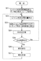
- the information in the internal storage unit 16a is also used to determine the necessity of executing the optimum index generation 11. This necessity determination corresponds to various changes in production process # 1 to be managed (changes in processing capacity of equipment group, change in target production rate, change in traffic, change / addition of Q-time constraints, etc.) To be judged. If the necessity is confirmed, a calculation instruction is given to the optimum index generation 11.
- the index calculation unit 17 outputs the calculation result of the CKB optimum logical value calculation unit 15 to the production management system 10 in an appropriate data format, the information of the internal storage unit 16a of the sensitivity analysis unit 16 and the current CKB optimum logical value It also has a function of sending update data to the production management system 10 more quickly by comparing the calculation conditions of the calculation unit 15.
- the sensitivity analysis unit (performance characteristics) 18 inputs the input data used for the CKB method, the conditions of the CKB optimal theoretical value, and under the conditions of the determined CKB optimal theoretical value, the process for evaluating the performance of the process Calculation is performed, and various performance evaluation indexes for traffic intensity, arrival rate, and process capacity are output to the production management system 10 as performance characteristics.
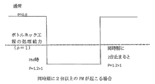
- the optimal load rule determination unit 19 determines the boundary of arrival ratio ⁇ ⁇ L such that TB ⁇ T_ (Q +) at which the magnitude relation between batch set waiting time TB related to product arrival and Q-time constraint (upper limit) T_ (Q +) switches.
- the value L is calculated and an appropriate load rule is determined.
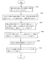
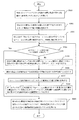
- Information on a plurality of devices included in the production execution system is input by the information input unit 12 via the production management system 10, and Q-time indicating a limit value of staying time between processing steps by the plurality of devices based on the input information
- Q-time indicating a limit value of staying time between processing steps by the plurality of devices based on the input information
- the structure of the constraint is analyzed by the Q-time structure analysis unit 14, and the number of optimal Kanban and the buffer size for each product type are calculated based on the input information and the Q-time structure, and the index calculation unit 17 is used as index information. Then, the optimum index information calculated by the index calculation unit 17 is supplied to the production management system 10.
- Q-time constraints can be obtained by providing analysis methods and appropriate management methods for handling of multi-variety production and mutual interference of multiple Q-time constraints, which are the main causes of Q-time constraint cracking. It is possible to simultaneously achieve improvement in non-defective product throughput, cost reduction and environmental load reduction while complying with the requirements.
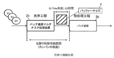
- the optimum index generation device 11 sets, for example, a Q-time constraint section of the pre-semiconductor step shown in FIG. 2 as a control target.
- This process section is a process section in which the cleaning process and the heat treatment process are continuous, and the following can be mentioned as its features.
- the control target of the optimum index generation device 11 is treated as a Q-time constraint section of the semiconductor pre-process, the present invention is not limited to such a target. It can be applied to the information communication process.
- this process section may become a bottleneck of the entire production execution system due to the existence of Q-time constraints, it affects the throughput.
- the load size (batch) determined by the load rules affects the throughput, the utilization of the apparatus, and the cost for processing per unit product.
- the product has various processing units such as "part (wafer)""lot""batch".
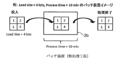
- part (wafer)""lot""batch the plurality of lots that can be processed are collectively called a batch.
- the maximum number of lots that can be processed simultaneously (batch size) varies depending on the process.
- the batch size of the cleaning process targeted by the present embodiment is 2 lots, and the batch size of the heat treatment process is 6 lots.
- a processing line in which steps capable of processing in batch units are continuous is called "batch processing line". The washing step and the heat treatment step will be described later.
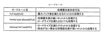
- the load rule is a rule that determines the batch group policy, such as whether it is possible to start processing if there are many lots in the batch processing apparatus, and if the specifications (processing conditions) are the same even for other types.
- the production target and the performance evaluation index in the process of the representative Q-time constrained section shown in FIG. 2 will be described.
- the important production targets in the factory are (1) Maximize Q-time compliance rate (2) Maximize delivery time rate (3) Maximize throughput (4) Maximize setup cost (5) Optimization of equipment utilization rate (6) Minimize total cost It is.
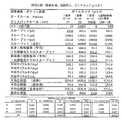
- production targets (1), (2), (3), (5) and (6) are taken up. Key performance indicators and their calculation methods to achieve these goals are shown in FIG.
- FIG. 4 is a diagram showing a batch continuous multitasking processing apparatus (cleaning step). In the cleaning process, an apparatus called a batch multitask (batch multichamber) type is used. As shown in FIG.
- the batch multitasking (batch multi-chamber) type has a plurality of washing tanks (referred to as units) in one apparatus, and a series of sequences determined by processing conditions of batches. When finished in the (tank), the batch is expelled from the apparatus. Therefore, the processing time from the start of processing in the apparatus to the end of processing differs from the interval between the input of batches to the apparatus and the output of batches from the apparatus.
- processing proceeds through a plurality of predetermined units while WIP (batch) is stored in the apparatus in units of units. Batches are loaded at Load Interval, not at processing time interval. Generally, the processing capacity of the cleaning process is considered to be higher than that of the subsequent heat treatment process.
- FIG. 5 is a view showing a batch apparatus (heat treatment step).
- a batch In the heat treatment process, an apparatus called a batch is used.
- this batch device refers to a device capable of batch processing. Further, in this apparatus, lots can be input at processing time intervals.
- a queue In a batch processing line in which apparatuses (processes) loaded with different batch sizes are continuous as described above, a queue is also generated by a batch set. Also, the load time changes the waiting time of the batch groups, so the staying time changes.
- Kanban method and queue theory are applied to consider a production scheduling method for suppressing deterioration of other process performance while observing Q-time constraints in a batch processing line.
- Little's formula which is particularly applied in Kanban method and queuing theory as prior knowledge will be described.
- Kanban system is an inventory system as a part of the Toyota production system, in particular the just-in-time system, and so-called “post-replenishment” This is a dependent demand version of a kind of quantitative ordering system, which is based on the method of returning to the inventory amount.
- Kanban used in the present embodiment refers to “repeatable Kanban” used for production instructions.
- the basics of the Kanban method are "back-end process taking", that is, “the part requiring the downstream process needs to go to the upstream process as needed”. In other words, it is not permitted for the front-end process to start and ship production without instruction of the back-end process. It is also called “pull system” (pull system) in the sense that it pulls from the post process.
- the CKB method which is a physical distribution control method for Q-time constraint compliance, will be described below.
- Q-time constraint compliance and in-process upper limit In this embodiment, as an overall function of the production system, consider a production scheduling method that does not deteriorate other performance evaluation indexes while keeping Q-time constraints. Q-time constraint cracking occurs as a result of WIPs being processed one after another in the cleaning process and arriving at the heat processing process without considering the throughput of the heat processing process, and a large number of WIPs waiting in front of the heat processing process. Therefore, it is considered that the Q-time constraint cracking can be suppressed by limiting the number of waiting WIPs in advance and waiting before the cleaning step in consideration of the processing capability of the heat treatment step. In order to realize that, from Little's formula in the theory of queuing, we calculate the maximum number of works that can comply with Q-time constraints, and also consider control of the number of works in progress by Kanban method.
- the maximum work in process limit is performed in three steps. Detailed methods will be described later. (1) Calculate the maximum number of waiting lots that can comply with the Q-time constraint using Little's formula. (2) Based on the maximum number of waiting lots, the number of pieces of paper is determined so as to control the amount of work from the cleaning process to the heat treatment process.
- the number of pieces of Kanban is set for each kind (spec)
- the CKB- (minus) method the number of pieces of Kanban is collectively set in the process without discriminating the kinds. It was decided to use it to confirm the effect of managing by breed.
- W is the margin time of Q-time constraint time
- ⁇ is the arrival rate of the heat treatment process (however, when traffic intensity ( ⁇ ) is larger than 1, ⁇ is arrival when traffic intensity is 1 Rate) and the maximum number of waiting lots Ask for This represents the maximum number of lots that can be waited for before the heat treatment step.
- Traffic intensity ( ⁇ ) (arrival rate ( ⁇ )) / ⁇ (service rate ( ⁇ )) ⁇ (number of devices (m)) ⁇
- Batch device service rate ( ⁇ ) (load size) / (average processing time)
- Batch continuous multitasking device service rate ( ⁇ ) (load size) / (load interval LI) (3)
- the number of Kanban will be decided based on the maximum number of waiting lots obtained above.
- the number of lots in the work-controllable section by Kanban includes not only the maximum number of waiting lots but also the number of lots being processed in the cleaning process. Therefore, the number of pieces of paper must be determined in consideration of the number of lots being processed in the washing process on average.
- the average number of lots in the cleaning process is determined by the following equation.
- FIG. 6 is a diagram showing the in-process control section.
- FIG. 7 is a diagram showing a typical load rule.
- FIG. 8 is a diagram showing batch set waiting time (factor).
- the Little's formula assumes processing for each lot, so there is no time to wait for the batch set generated by batch processing. In batch processing, processing is performed not for each lot but for each load size (batch). Thus, as shown in FIG. 8, when the lot arrives at the heat treatment step from the cleaning step, it will wait extra for the defined load size to be reached beyond the waiting time defined by Little's formula. The waiting time required before starting this batch processing is called batch set waiting time.
- the maximum batch set waiting time for the first arriving lot of the batch set to wait is determined for each load rule of the heat treatment process. Also, the prescribed load size depends on the load rule.
- the load rules used in this embodiment are shown in FIG.
- FIG. 9 is a diagram showing batch set waiting time (calculation).
- A In the case of "Washing process: Full load heat treatment process: Full load” TB waiting time for batch assembly [minutes], L1: Load size of washing process equipment [lot / unit], L2: Heat treatment process loading Size [lot / unit], L2 / L1 the number of arrivals from the washing process to meet the processable load size of the heat treatment process equipment, ⁇ wash the arrival rate of the washing process [lot / min], L1 / ⁇ Assuming that the arrival interval of the lot from the process [minute / lot], as shown in FIG. 9, the lot arriving at the arrival interval (1 / ⁇ ) in the cleaning process is processed with the load size L1 and the arrival interval (L1 / ⁇ ) Arrive at the heat treatment process in
- the batch set waiting time changes according to the load rule.
- the number of Kanban is calculated by the following calculation.
- N * (TQ-max (TB, TQ-)-E) ⁇ ⁇ (8)
- N ** N * + LW (9)
- the number of kanban is represented by. However, when the traffic intensity ( ⁇ ) is larger than 1, ⁇ is the arrival rate when the traffic intensity ( ⁇ ) is 1. Further, in a section that is rate-limited by the following Q-time constraint that interferes, the number of Kanbans is calculated by equation (10).
- Buffer size Buffer size is used to further ensure logistics control for Q-time constraint compliance.
- the number of in-process items that can be controlled by the Kanban method is only the sum of the number of waiting lots in the heat treatment process and the number of in-process lots in the cleaning process. Therefore, if the washing process has higher throughput than the heat treatment process, all the lots processed in the washing process are output early, and all the lots given the load are the waiting lots of the heat treatment process. Sometimes it becomes. In such a case, the maximum number of lots that can be waited before the heat treatment process determined by Little's formula is exceeded, resulting in rework. In actual factories, it is considered that such a situation often occurs because the cleaning process generally has higher throughput than the heat treatment process.
- the buffer size is not necessarily required since the time for which the apparatus of the heat treatment process is idle does not occur in the case where the magnitude relationship of the processing capacity is reversed. Note that this is not the case in the case of responding to fluctuations in production distribution or in the third embodiment.
- a buffer size is provided before the heat treatment step, and the number of waiting lots is limited so as not to exceed the maximum number of lots that can be waited before the heat treatment step determined by Little's formula.
- the reason for defining the buffer size in this way is that taking into consideration the batch set waiting time, as a result, Q-time restriction cracking (occurrence of rework etc.) is suppressed even if it is not originally required to stop the cleaning process. To prevent the cleaning process from being stopped regardless of the situation.
- the average number of lots in the cleaning process is 11 and the maximum number of waiting lots for the heat treatment process is 86 lots, taking batch group waiting time into consideration, and the maximum waiting lot for the heat treatment process not taking batch group waiting time into consideration
- the number is 90
- the number of cards is 97 and the buffer size is 90 lots.
- the buffer size is set to 86 lots and the number of lots waiting for the heat treatment process is 86 lots, the washing process is stopped even though the Q-time constraint cracking does not occur even if the cleaning process is operating. It will In order to prevent such a situation, the buffer size is set to 90 lots of the maximum waiting lot number of the heat treatment process which does not take batch set waiting time into consideration.
- the buffer size is defined in units of processes. When multiple types are mixed, a buffer size is obtained for each type, and the sum is used as the buffer size. That is, assuming that B * is a buffer size [lot], TQ is a queue time (maximum stay time) [minutes], and ⁇ i is an arrival rate of variety i [lot / minute]
- the buffer size is represented by.
- n is the number of varieties.
- the control of the upper limit of the number of works in progress by the buffer size forcibly stops the previous process (in this case, the washing process) (waiting for processing), this is not desirable for smooth production.
- it is positioned as a function used to more reliably control Q-time compliance by the Kanban-type in-process number.
- the upper limit of the number of in-process products is calculated by the above procedure. Also, in a Q-time constraint section in which multiple Q-time constraints interfere, the preceding Q-time constraint limited by the subsequent production process (hereinafter referred to as the bottleneck process) with the lowest production rate The calculation method of the number is different.
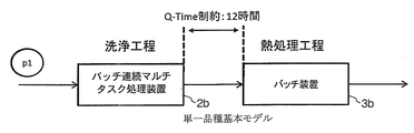
- FIG. 10 is a diagram showing a single-breed basic model.
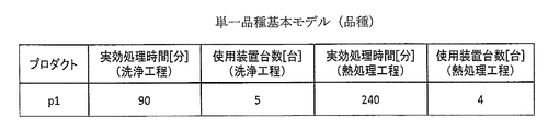
- FIG. 11 is a diagram showing a single-kind basic model (step).
- FIG. 12 is a diagram showing a single-type basic model (type).
- a batch processing line of washing process and heat treatment process one kind, four apparatuses of washing process and plural apparatuses of five apparatuses of heat treatment process are assumed. Perform simulation experiments.
- the cleaning process is composed of a batch / multitask type apparatus group, the effective processing time is 90 minutes, the other heat treatment process is composed of a batch apparatus, and the effective processing time is 240 minutes. Further, as shown in FIGS. 11 and 12, the batch size and the number of apparatuses are also different.
- the experiment is performed by changing the arrival rate using the model as described above.
- the arrival rate of the varieties was 0.3, 0.6, 0.8, 1.0, 1.2, 1.5, and the traffic intensity (utilization rate) of the smaller processing capacity of the two processes of cleaning and heat treatment was 0.3 I decided to become.
- simulation experiments will be conducted for two cases: periodic injection and index injection.
- the arrival rate is determined based on the traffic intensity of the heat treatment process because the heat treatment process has smaller throughput than the heat treatment process.
- a model that is set to rework when the Q-time constraint is broken, and a model that sets the calculated number of buffers and buffer size to the QT model (( CKB method) and 3 of the conventional model (CT) which determines whether the Q-time constraint can be observed or not from the device status and the number of WIPs (number of works in progress) at the start of processing and determines whether or not the product can be released.
- CKB method CKB method
- CT conventional model
- WIPs number of works in progress
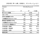
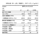
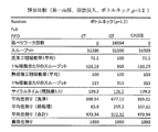
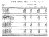
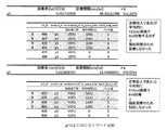
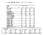
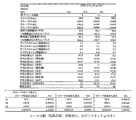
- FIG. 13 and FIG. 14 show the result in the case of regular injection
- FIG. 15 and FIG. 16 show the result in the case of index injection. Here, those with good performance are underlined, and those with poor performance are shown in bold.
- the cycle time is large in the CKB method and CT model values, which is considered to be the result of the output lot being intentionally put on standby before the cleaning step.
- the throughput does not decrease, so the performance does not necessarily deteriorate.
- cost performance is rather improved because the same amount of throughput can be realized at a lower operation rate than both the CKB method and the CT model and the QT model.
- FIG. 17 is a diagram showing a multi-kind basic model.
- FIG. 18 is a diagram showing a multi-kind basic model (step).
- FIG. 19 is a diagram showing a multi-product basic model (product).
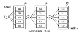
- FIG. 20 shows a processable device (washing).
- FIG. 21 is a view showing a processable apparatus (heat treatment).
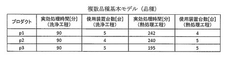
- the cleaning process is composed of a batch sequential type of apparatus group, and the other heat treatment process is composed of a batch apparatus, and as shown in FIGS. 20 and 21, the batch size and the number of apparatuses are also different.
- the effective processing time and the number of devices used differ depending on the product type. For the type 1 (p1), the effective processing time of the cleaning process is 90 minutes, the number of devices used is 5 and the effective processing time of the heat treatment process is 242 minutes, the number of devices used is 4 .
- the type 2 (p2) is 90 minutes of effective treatment time of the cleaning process, 4 units of equipment used, 240 minutes of effective treatment time of the heat treatment process, and 5 units of equipment used.
- Type 3 is the effective processing time of the cleaning step of 90 minutes, the number of devices used 5 units, the effective processing time of the heat treatment step 195 minutes, the number of devices used 5 units. Moreover, the apparatus which can process each kind is decided. In the cleaning step, as shown in FIG. 20, the devices used by p1, p2 and p3 are different. Also in the heat treatment step, as shown in FIG. 21, there are devices that use different types of p1, p2, and p3.
- the experiment is performed by changing the arrival rate using the model as described above.
- the traffic intensity (utilization ratio) of the smaller of the two processes of washing and heat treatment is 0.3, 0.6, 0.8, 1.0, 1 as in the experiment in the previous section. Decide to be .2 and 1.5.
- all traffic intensities ( ⁇ : utilization rate) are those of the heat treatment processes.
- the effective processing time and the number of usable devices are different for each type, so it is necessary to separately obtain the arrival rate. As shown in FIG.
- Tp processing time
- FIG. 22 is a diagram for explaining the determination of the input rate.
- (1) If >> 1, calculate with ⁇ 1 (2) Calculate the input ratio of each product from the production ratio of each product in each shared device (3) Input ratio in all devices for each product (4) Calculate the input rate of the breed from the combined feed rate Based on these things, set the same number of QT and CT models as before and the number of buffers for each breed, and buffer size
- the model of CKB method is provided, the number of Kanban is set in the whole process without providing discrimination for each type, and experiments are performed on four models of the model of CKB-method with a buffer size, and the performance is compared.
- the CKB method suppresses Q-time constraint cracking in both cases where the traffic intensity is 0.8 and 1.2.
- Q-time constraint cracking has occurred in all models when the traffic intensity is 0.3 and 0.6 in the case of index input.
- the underlying QT model has higher throughput per 1% operation of the cleaning process, but lowers that of the heat treatment process. This is considered to be due to the fact that the heat treatment process, which should have been a bottleneck, has not been sufficiently operated, and it can be said that the performance is deteriorated in view of the entire plant. Above all, a lot of rework (32%) is not good for performance.
- the CT, CKB and CKB-methods show no deterioration in the average work-in-process performance compared to QT.
- the difference in final work in process is represented by the difference in throughput being converted into lots. This difference is considered to be the result of uneven processing of varieties.
- the percentage of processing including rework is higher for both CKB and CKB than for CT and QT, and the overall throughput is higher for all of CT, CKB, and CKB than for QT. None of the throughput per 1% operation is worse than QT. It can be seen that the overall average is not worse than QT, although the cycle time and average work-in-process vary among varieties.
- experiment is performed by changing the load rule. The description of each load rule is shown in FIG. In the previous experiments, all load rules have been done at full load.
- the experiment is performed by changing only the load rule of the heat treatment process.
- the model to compare compares three models of the load rule of the heat treatment process with Full, PLA, and AFL.
- the traffic intensity was 0.3
- the number of Kanban p1 at Full became 4 smaller than the batch size 6 lots of the heat treatment process. Therefore, the same experiment was performed with a model (p1Full4) in which only p1 was set to process 4 lots.
- the traffic intensity is 0.6 or more
- the p1Full4 model has more than six Kanbans, and all settings and results are the same as Full.
- the experiment was performed by determining the arrival rate based on the traffic intensity of the heat treatment process as before. The results are shown in FIG. 27, FIG. 28 and FIG. 29 by extracting the cases with traffic intensities of 0.3, 0.8 and 1.2 among them.
- the present embodiment focuses on Q-time constraints that are of high importance in semiconductor manufacturing, and takes Q-time constraint sections of continuous processes of batch processing of cleaning and heat treatment processes that are particularly pointed out.
- the prior art on Q-time constraints to the present is insufficient in precision and accuracy, and the effects on other performance indicators other than Q-time constraint compliance have not been considered.
- a CKB method is developed to control the upper limit of the number of in-process items in Q-time constraint sections, and It was evaluated by stochastic simulation experiments.
- the CKB method has high reliability and versatility because it theoretically calculates the number of Kanban and the upper limit of the number of works in progress based on the Kanban method and queuing theory. In addition, it has been confirmed that the effect is exhibited particularly in a situation where the process utilization rate is 60% or more, which is particularly high in ordinary factories.
- a simple change such as a load rule ensures even for a low arrival rate condition (such as traffic intensity 0.3), which is the second cause of Q-time constraint cracking.
- a low arrival rate condition such as traffic intensity 0.3
- Q-time constraint cracking may occur due to the setting of a load rule or the like.
- the optimal load rule determination unit 19 determines the boundary of arrival ratio ⁇ ⁇ L such that TB ⁇ T_ (Q +) where the magnitude relation between batch set waiting time TB and Q-time constraint (upper limit) T_ (Q +) changes in consideration of arrival variation. Calculate the value L and use appropriate load rules. If ⁇ (L, Full load (force a full size batch set). If ⁇ ⁇ L, use a method such as PLA or AFL that does not force full-sized batch sets. In the present embodiment, in addition to the case where the arrival rate is low and there is variation, the arrival rate differs depending on the product type and the process, and is considered.
- the determination of the number of Kanbans and the buffer size used in the present embodiment can be calculated at high speed and with high accuracy with respect to fluctuations in arrival rate and processing capacity, and surely Q- Time restriction can be prevented.
- the qualitative evaluation such as calculation speed, accuracy and practicability also achieves the purpose through the construction and performance evaluation of the high CKB method. We were able to.
- the first problem is solved by the CKB method.
- a practical production logistics method that achieves high throughput while complying with Q-time constraints in multi-variety production is named CKB (Control of Kanban and Buffer sizes).
- CKB Control of Kanban and Buffer sizes
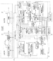
- the optimal index generation device 21 according to the second embodiment of the present invention manages, for example, the maintenance schedule of the device group 5 provided in each of the production process # 1 with respect to the operation method for dispersing the preventive maintenance time of the manufacturing device
- the production management system 10 and the engineering business system 29 are targets of control.
- a production load distribution method hereinafter referred to as the JAMP method for dispersion of maintenance time will be described.
- the optimum index generation device 21 includes an input unit 22, an auxiliary input unit 23, an apparatus classification calculation unit 28, a JAMP optimum logical value calculation unit 24, a sensitivity analysis unit (JAMP characteristic) 25, and calculation of start and end times.
- a unit 26 and a sensitivity analysis unit (performance characteristic) 27 are provided.
- the input unit 22 receives maintenance time from the production management system 10 and the engineering operation system 29, maintenance guidelines (number of processes before start of maintenance in fixed maintenance, maintenance cycle in regular maintenance, etc.), number of devices in a group of processes (processes) Enter the production quantity or arrival rate by product type of the group (process), the processing time by product type / process / device, product type information that can be processed by the device, and the device type.
- the auxiliary input unit 23 receives setup time, information on batch type devices (batch size, load rule, load size, load interval) from the production management system 10 and the engineering operation system 29, information on multitask type devices (standby point in the device) All the information (device type, number of devices, processing time, production quantity or arrival rate by type of device group (process), type information that can be processed by the device) also available from the input unit input.
- the auxiliary input unit 23 inputs non-essential input data, but in practice, the important data are put together in the next stage of the JAMP optimum logical value calculation unit 24 and preprocessed to set up the setup time (product types, devices, Information on batch equipment, information on batch equipment (average load size, load interval, batch assembly time, equipment execution service rate), MTBF (average failure interval), MTTR (average repair time), information on multitasking equipment (equipment Output the presence / absence of standby and capacity value etc.
- the JAMP method optimum theoretical value calculation unit 24 performs more detailed calculation.
- the JAMP optimum logical value calculation unit 24 inputs the maintenance time, the maintenance guideline, the number of apparatuses, the production quantity or arrival rate by product type, the processing time by type, process / apparatus, the type information processable by the apparatus, the apparatus type Based on the setup time, and other information related to the device, the processing load (number of times) of each device and the processing timing thereof are calculated and output as the JAMP theoretical value calculation result.
- the sensitivity analysis unit (JAMP characteristic) 25 calculates the JAMP theoretical value calculated from the JAMP optimum logical value calculation unit 24 and calculates the JAMP theoretical value when the processing load (number of times) of each device and its processing time fluctuate.
- the sensitivity analysis unit (JAMP characteristic) 25 records this sensitivity analysis result in the internal storage unit 25a, and the processing load (number of times) of each device and its processing time dynamically change as the JAMP theoretical value calculation result If it does, it can also be used immediately as update data.
- the start / end timing calculation unit 26 inputs lot information and engineering information to be processed, and calculates start / end timing of processing and preventive maintenance of each device from the calculation result of the theoretical value of the JAMP method. Then, the start and end times of the processing and preventive maintenance of each of the regular device and the alternative device are output as the preventive maintenance schedule.
- the sensitivity analysis unit (performance characteristic) 27 inputs the input data used for the JAMP method, the conditions of the JAMP method optimal theoretical value, and under the conditions of the determined JAMP method optimal theoretical value, for the evaluation of process performance Calculation is performed, and as a performance characteristic, traffic intensity v. s.
- the various performance evaluation indexes are output to the production management system 10.
- the device category calculating unit 28 divides the device into a regular device and a substitute device (a regular ability and a substitute capability), and outputs device classification information.
- the regular device refers to the device capability that is constantly required to avoid long waiting lots
- the alternate device refers to the other average surplus capabilities.
- the ordinary ability is ⁇ / ⁇
- the ordinary device is It becomes a stand.
- the alternative capacity is (m ⁇ / ⁇ ) and the alternative device is It becomes a stand.
- the engineering service system 29 is a system that manages and manages tasks such as preventive maintenance and failure handling of production facilities, and manages conditions, schedules, and results of general engineering tasks that are not held in the production management system 10. For example, there are master information such as a range of responsibility of a device engineer, execution conditions such as shift, and performance data of preventive maintenance and failure handling. Depending on the production management system, the engineering business system 29 may be incorporated as a function of the production management system 10.
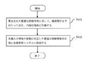
- Information on a plurality of devices included in the production execution system is input by the input unit 22 through the production management system 10, and the device category calculating unit 28 substitutes a plurality of devices into a regular device having regular capability and an alternative capability. It divides into the device and calculates the number of times of operation and the operation time of multiple regular devices and alternate devices (and regular capabilities and alternate capabilities) from the device capability classification and input information, and preventive maintenance for regular devices and alternate devices.
- the start / end timing is calculated by the start / end timing calculation unit 26, and the optimum start / end timing information calculated by the start / end timing calculation unit 26 is supplied to the production management system 10 or the engineering operation system 29.
- Q-time constraint compliance can be achieved by providing an analysis method and an appropriate management method.
- preventive maintenance As compared with the time spent for post-maintenance to restore normal condition after equipment condition is broken or abnormal, it is the operation time of equipment as a result of maintenance of equipment before failure or abnormality occurs.
- PM preventive maintenance
- regular maintenance is often performed to perform predetermined maintenance at regular intervals, but for devices that perform chemical physical processing, quantitative maintenance that performs maintenance according to the number of times of processing is performed.
- fixed maintenance of a semiconductor factory is mainly taken up (note that it can be applied to periodic maintenance).
- Q-time constraints upper and lower limit values of residence time between machining
- Q-time constraint cracking is likely to occur in a situation where the waiting time is extended due to preventive maintenance (PM) of the manufacturing apparatus, so decentralization of the apparatus PM is a quality assurance and cost viewpoint It is also a very important task.
- a load distribution method is newly developed in which a semiconductor manufacturing process composed of a plurality of devices for performing maintenance in a fixed amount is taken, and jobs are allocated to the devices so as to reduce the number of devices that become PM at the same time.
- the purpose is to confirm the effect.
- the feature of fixed maintenance is that maintenance is started when the number of times processed by the device reaches a specified value. In other words, it is possible to control the allocation of WIPs to the devices to control the number of times of processing of each device, and to prevent the preventative maintenance periods of a plurality of devices from overlapping.
- the device is divided into a regular device and a substitute device, and the substitute device is used to decentralize the time of PM, and an extra waiting time for the job at any time other than PM.
- the substitute device is used to decentralize the time of PM, and an extra waiting time for the job at any time other than PM.
- the performance of the load distribution method is verified by simulation experiments with reference to the actual factory process model (the process of processing one product with a given processing time with six devices, regular input).
- comparison is made with simple parallel rules that use devices sequentially without intentional load distribution.
- PM can be completely dispersed by suppressing the number of devices that become PM in the same period to 1 or less at the same time by the load distribution method, and in the case where PM can not be completely dispersed in one cycle.
- the waiting time of the lot by PM becomes long, and it becomes easy to occur a situation where rework occurs by breaking the Q-time constraint.
- the occurrence of rework is only a loss on production and is undesirable.
- the lot single task type device refers to a device in which the processing unit of the device is one WIP (for example, a lot) as shown in FIG. After the predetermined processing time has elapsed, the WIP is swept out, and when it is idle, processing of the next lot can be started.
- [Performance evaluation index] There are various performance evaluation indexes to aim at the ability of the factory in the semiconductor production line. The performance evaluation indicators taken up in this research and their definitions are shown.
- the total [minutes] of waiting time is calculated as the sum of the waiting time occurring in each lot, and should be smaller.
- the waiting lot number [lot] is calculated as the total number of lots in which waiting time has occurred, and should be smaller.
- the Q-time constraint split lot number [lot] is calculated as the number of lots that have become Q-time constraint split, and it is better to be smaller.
- FIG. 32 is a diagram showing an example of fixed maintenance.
- a method of performing maintenance every time processing is performed by 100 lots in the example of the figure is called fixed maintenance each time the apparatus reaches the number of times of processing (number of lots) set in advance.
- the feature of fixed maintenance is that maintenance is required when the number of times processed by the device reaches a specified value. In other words, it is possible to control the allocation of WIPs to the devices to control the number of times of processing of each device, and to prevent the preventative maintenance periods of a plurality of devices from overlapping.
- FIG. 33 is a view showing a group of devices (m1 to m6) in a normal state.
- FIG. 34 is a diagram illustrating when the device m6 substitutes m2 during preventive maintenance (except m1, m3, m4, m5, and m6 except WIP2).
- JAMP load distribution method
- PM newly considered fixed maintenance
- the entire configuration of the newly developed rule will be described using an actual factory process model.
- the traffic intensity ⁇ / M (indicating the degree of process congestion), which is the ratio of the arrival rate ⁇ ⁇ ⁇ of a job to the process and the service capacity M of the process, is 1 ( Equipment planning and load planning are being conducted to be smaller than 100%. In other words, there is surplus service capacity.
- the traffic intensity of this process is 0.8, and the number of devices required to process the job is theoretically 4.8, that is, 5 devices.
- One remaining device can be used as an alternative device.
- FIG. 35 is a diagram for describing the case where two or more PMs occur at the same time.
- FIG. 36 is a diagram for describing the case where only one PM occurs at the same time.
- regular devices normally used devices
- a time (MTTR: Mean time to repair) in which the device is PM occurs.
- MTTR Mean time to repair
- the traffic intensity drops below one, the traffic intensity exceeds 1 (FIG. 35). It is known that when the traffic intensity is larger than 1, the job waiting time increases rapidly. The increased latency has a negative impact on cost increase, on-time delivery and Q-time constraint compliance.
- the number of devices in the process is m
- the feature of fixed maintenance is to start maintenance when the number of times processed by the device reaches a specified value.
- a method will be considered in which the time of PM is dispersed using an alternative device, and an unnecessary waiting time is not generated in the job at any time other than PM.
- the case of six devices shown in FIG. 33 will be described as an example.
- condition (1) and condition (2) Under the combination of condition (1) and condition (2), if the number of times of alternative processing of the alternative device is equal to or less than the specified number starting PM, PM of the regular device can be completely dispersed (the number of devices that become PM at the same time) It can be reduced to the number of substitute devices or less). If this condition is not satisfied, the number of devices requiring maintenance at the same time must be greater than (m ⁇ [ ⁇ / ⁇ ]) units, which causes additional waiting time for the job. As described above, when the conditions (1), (2) and (3) are satisfied, it is possible to completely disperse the normal device and the alternative device PM in one cycle. Even when the system can not be completely decentralized, load balancing is performed as much as possible to shorten the overlapping period of the PM timing.
- the case where the conditions (1) and (2) are not completely satisfied corresponds to the case where the overlapping time of the PMs of all the regular devices can not be zero in one cycle.
- one cycle refers to a period from when the first device (m1) starts operating until all the regular devices finish PM one by one. For example, it corresponds to the case where the time length of MTTR is relatively long.
- load distribution by the JAMP method is applied as much as possible to reduce and disperse PM overlap time.
- substitute processing is performed within the range of conditions to achieve complete dispersion.
- FIG. 37 is a diagram showing simple parallel processing.
- FIG. 38 is a job allocation diagram in consideration of fixed maintenance. [Requirements for decentralizing PM]
- the above-mentioned conditions (1), (2) and (3) will be described in detail.
- the condition (1) in the case of the model shown in FIG.
- ⁇ j is the arrival rate per apparatus j [lot / min]
- ⁇ is the lot arrival rate to the process [lot / min]
- ⁇ is a single Average service rate of equipment 1 / Tp [lot / min]
- ⁇ j ⁇ / [ ⁇ / ⁇ ]
- N is the reference value for quantitative maintenance [lot]
- MTTR j is the time required for preventive maintenance (PM) of apparatus j [minutes] (the apparatus is stopped during this period, and the production lot Can not process).
- the number of commonly used devices is [ ⁇ / ⁇ ] and the number of alternative devices is (m ⁇ [ ⁇ / ⁇ ]).
- the condition (1) is expressed by
- condition (1) in the model shown in FIG. 38, m6 performs m2 to m5 alternative processing for preventing other devices from becoming PM during the PM period of m1, and the total time is the condition (1), which indicates that the alternative process shown on the left side of the condition (1) has ended before the start of the m1 PM.
- condition (2) means that the alternative device does not start PM for a period from when the first device starts PM until the devices until [ ⁇ / ⁇ ] th device finish PM.
- the right side of FIG. 38 shows this alternative.
- Condition (2) is expressed as the following equation.
- the condition (3) is to be able to adjust the assignment of the job of the alternative device so that the PM of the alternative device and the PM of the other device do not overlap.
- the following two cases are considered separately.
- the remaining number of possible alternative at the end of the (k ⁇ 1) period is expressed by the left side of the following expression. Since the number of alternative times must be a positive value, the following condition is satisfied.
- the alternative device becomes PM in a cycle in which the remaining number of possible replacements shown on the left side is smaller than the number of required replacements in the next one cycle.
- the total number of times of substitution for the other regular devices (m2, m3, m4 and m5 in the example shown in FIG. 40) is N'-N'1.
- the PM end in the regular use apparatus first (m1 in the example shown in FIG. 40) ends the PM in the regular use apparatus (m5 in the example shown in FIG. 40) the PM ends last
- the number of lots processed by the time is expressed by the following equation.
- the number of lots that can be processed by the first PM device among the regular devices is
- the PM of the alternative device does not overlap with the PM of the regular device.
- the equation becomes the condition of [2] of the condition (3).
- the JAMP method can distribute PMs so that the traffic intensity does not exceed 1. First, it is checked whether these conditions are satisfied. If satisfied, the timing of PM can be decentralized by causing the alternative device to pre-process a predetermined number of alternatives.
- Condition (1) is
- Condition (3) [1] is
- FIG. 41 is a diagram for describing an apparatus operation guideline 1 in the case where complete decentralization can not be performed in one cycle. Based on the concept of the JAMP method, the load is distributed using an alternative device, and the number and the length of time to become PM at the same time are suppressed as much as possible. However,
- the lot can not be substituted in the same cycle (for example, the first cycle).
- FIG. 41 is a diagram for describing an apparatus operation guideline 2 in the case where complete decentralization can not be performed in one cycle.
- the overlapping time lengths are dispersed so that overlapping periods of PM periods are not as continuous as possible.
- FIG. 42 is a diagram for describing complete decentralization (after the second period) of the pointer 3. Eliminate the overlapping time of the PM period, including R batches that could not be completely substituted in the first cycle.
- the deviation is shifted backward to achieve complete dispersion.
- substitution is made within the range satisfying the conditions of the JAMP method (It is not always possible to achieve complete dispersion in the second cycle. Dispersion is achieved using a necessary cycle).
- the purpose of this simulation experiment is to distribute the load to each device in advance in consideration of quantitative maintenance when simply parallel processing is performed (hereinafter referred to as a simple parallel rule) in the process where a plurality of devices exist. By comparing the performance of JAMP rules, it is to confirm the effect of JAMP rules.
- a simulation experiment is performed on the assumption of one lot and six lot single task type devices shown in FIG.
- the lot single-task type apparatus refers to an apparatus that processes one lot at a time. Lots shall arrive at regular intervals according to the traffic intensity by periodic injection. For operation based on the simple parallel rule of six devices, when traffic intensity is 0.8, normally five devices are used as shown in FIG. 33, and when any device can not be used by PM etc. Use the remaining one as.
- FIG. 43 is a diagram showing set values of a model.
- FIG. 43 shows the processing time, the process traffic intensity, the number of lots (PM pointer lot number) serving as a guideline for starting quantitative maintenance, and the time required for preventive maintenance (MTTR).
- MTTR time required for preventive maintenance
- two conditions (S1, S2) where the conditions (1) and (2) of the JAMP rule can be met, and cases where the combined condition of the conditions (1) and (2) can not be met (S3) Use a total of three scenarios.
- the difference between the scenarios S1 and S2 is that the PM of the alternative device occurs at the end of the PM of the regular device in S1 and corresponds to [1] of the condition (3).
- S2 if PM of the alternative device does not make any adjustments, it will overlap with the timing of PM of other devices, and it is necessary to apply the condition (3) [2] to suppress the occurrence of waiting time ing.
- S3 is always a case where two or more PMs need to be generated simultaneously. S3 corresponds to the actual factory PM condition setting (stopped for 24 hours for every PM after 100 lot processing). Using the above model, we will experiment with two rules, simple parallel and JAMP, and compare the results.
- FIG. 44 is a diagram for describing setting of the number of alternatives in JAMP.
- m1 to m5 up to the 100th lot except for the first five m1, m2,.
- the parallel processing is simply performed on the table, and during one of the first to fifth PMs, the device that can start processing the fastest among m6 or other devices substitutes for the processing.
- the JAMP rule is a rule in which job substitution processing is performed in advance while considering fixed maintenance, and PMs are distributed, in addition to 1 / ⁇ deviation as in the simple parallel rule.
- the PM of five devices m1 to m5 can be substituted by causing the alternative device m6 to substitute the processing quantity of m2 to m5 before m1 starts PM.
- the load is distributed so that the number of PM paused devices is kept below 1 at the same time.
- FIG. 39 is an explanatory view of [2] of the condition (3) of the JAMP method.
- FIG. 43 shows the number of alternatives when using the JAMP rule under the set conditions of this experiment.
- one cycle refers to a period from when m1 starts processing of the first lot until m5 finishes MTTR (see FIG. 40).
- the scenario S3 corresponds to the case where the complete decentralization can not be performed in one cycle because it exceeds 100 of the PM guideline.
- FIG. 44 is a diagram for describing setting of the number of alternatives in the JAMP method.
- FIG. 51 is a diagram for explaining comparison between a simple parallel rule and a JAMP rule. With the settings shown in FIG. 43 and FIG. 44, simulation experiments were performed in three scenarios for two rules. The results until the end of the cycle in which the alternative device performs PM are shown in FIG. Here, three performance evaluation indexes were listed: the number of lots for which waiting by PM occurred, the cycle time, and the number of lots that exceeded the Q-time constraint.
- the results up to 9 cycles in S1 and the results up to 3 and 4 cycles in S2 and S3 are shown as the results up to the cycle for finishing load distribution and PM in the alternative device.
- the production period observation period
- the difference between simple parallel and JAMP expands in proportion to the values in the above table. From the above experimental results, it can be seen that in the JAMP rule, no waiting for a lot due to PM occurs in scenarios S1 and S2, and there is no lot that exceeds the Q-time constraint. In particular, it can be understood from the total waiting time that in the simple parallel rule, long waiting has occurred, while in the JAMP rule, waiting has not occurred.
- the JAMP rule distributes PMs to suppress the traffic intensity from becoming greater than 1 and suppress the occurrence of lot latency due to PMs, and lots that exceed the Q-time constraint. It could be confirmed that the occurrence of can also be suppressed.
- the alternative process for the condition (1) is performed by the alternative device in the first period and the PM is started in advance.
- the PM timing of the alternative device is processed between the devices because it does not overlap with the PM timing of the regular device Perform an operation to substitute for.
- the alternative device m6 shows the result in the case where it reaches 100 lots of the alternative device in the middle of the second and subsequent cycles and enters PM.
- the PM of the substitute device will also be started during the PM of the regular device, and a waiting lot will occur.
- Condition (3) [2] is required to address this case. Under this condition (3) [2], the MTTRs of multiple devices do not overlap by intentionally substituting other devices to adjust the PM timing of the alternative device even after the second cycle. It can be adjusted.
- the JAMP method is a method directed to leveling production, suppressing fluctuations by minimizing the decrease in process capacity due to PM. Therefore, in the subsequent process, the arrival of lots is equalized (FIG. 46: end time)
- FIG. 46 is a diagram showing time of arrival and departure of lot (comparison of JAMP method and simple parallel rule).
- the waiting time due to the PM can be reduced to zero, and even when the PM can not be completely dispersed, the number of devices in which JAMP becomes PM at the same time is possible.
- the waiting time of the lot due to PM becomes long, and it becomes easy to occur a situation where rework occurs by breaking the Q-time constraint.
- the occurrence of rework is only a loss on production and is undesirable because it obstructs the production flow of regular lots as a secondary matter.
- the traffic intensity of the process is always kept as low as possible by reducing the number of PMs at the same time, and no extra waiting time is generated. It has been confirmed that the number can be reduced.
- the proposed method can be used not only for quantitative maintenance but also for decentralization of regular maintenance.
- ⁇ j is the arrival rate per apparatus j [lot / min]
- ⁇ j ⁇ / [ ⁇ / ⁇ ]
- ⁇ is the arrival rate of the entire group of apparatuses [lot / min]
- PM preventive maintenance
- the conditions which considered the batch group time in a batch process become as follows.
- the processing start interval (load interval) and the processing unit (load size) differ depending on the load rule.
- the load interval when viewed from the device can be calculated as follows when the load size is La. Since the time interval for one lot to arrive is 1 / ⁇ , the time interval until one batch of size La is assembled is La / ⁇ .
- TL Tp when La / ⁇ ⁇ Tp / m (ie ⁇ 1)
- M is the number of devices
- Tp is the average processing time
- La is the average load size [lot]
- ⁇ is the arrival rate of the entire device group [lot / min]
- ⁇ j ⁇ / [ ⁇ / ⁇ ].
- the second problem is solved by the JAMP method.
- the method of allocating the load to the device to decentralize the preventive maintenance time of the device, which is the main cause of Q-time constraint cracking, was named the Job Allocation for Maintenance in Parallel (JAMP) method.
- JAMP Job Allocation for Maintenance in Parallel
- the second embodiment is the program of the JAMP method and the result of performance evaluation using it (by deterministic simulation using actual factory data).
- the optimum index generation device according to the third embodiment of the present invention will be described with reference to FIG.
- the optimum index generating device 31 according to the third embodiment of the present invention is, for example, the production of the processing step (device group) 2 and the processing step (device group) 3 respectively provided in production step # 1 for producing a semiconductor.
- a production management system 10 that manages a schedule is an object of control.
- the production management system 10 and the engineering operation system 29 for managing the maintenance schedule of the device group 5 respectively provided in the production process # 1 are targeted for control in the operation method for dispersing the preventive maintenance time of the manufacturing device.
- the production physical distribution control method and the production load distribution method hereinafter referred to as the CKB-JAMP method
- the optimum index generation device 31 includes the input unit 12, the auxiliary input unit 13, and the Q-time structure analysis unit 14 in the same manner as the optimum index generation device 11 (first embodiment) shown in FIG. Have.
- the optimum index generation device 31 has the input unit 22, the auxiliary input unit (JAMP method) 23, the start / end timing calculation unit 26, and the device classification similarly to the optimum index generation device 21 (second embodiment) shown in FIG.
- the calculation unit 28 is provided.
- the configuration characteristic of the third embodiment is, as shown in FIG.
- a fluctuation monitoring detection unit 32 an input change detection unit 33, a recalculation necessity determination unit 34, A sensitivity analysis unit (CKB + JAMP characteristic) 35, a CKB + JAMP optimum logical value calculation unit 36, and a sensitivity analysis unit (CKB + JAMP performance characteristic) 37 are included.
- the fluctuation monitoring and detection unit 32 monitors and detects fluctuations due to event and state data updates, such as lot processing start / end, equipment state change (due to failure etc.) and change in processing capacity of equipment group, etc. It is output to the calculation necessity determination unit 34.
- the input change detection unit 33 inputs CKB method-related input data and JAMP method-related input data, detects a portion changed from the previous CKB method-related input data and JAMP method-related input data, and there is a change. Output the input data.
- the recalculation necessity determination unit 34 inputs an integer threshold value in the sensitivity analysis result calculated in advance stored in the storage unit 34a and recalculates the variation detected by the input change detection unit 33. Determine if it is necessary.
- the recalculation necessity determination unit 34 determines that recalculation is necessary when it deviates from the upper and lower limit thresholds of the previous range.
- the CKB + JAMP optimum logical value calculation unit 36 receives input data from the Q-time constraint structure analysis unit and the input unit (JAMP method), and calculates the JAMP theoretical value for each device group in the Q-time restriction section. Calculate the processing load (number of times) and its processing timing, calculate the time transition of the processing capacity in the device group for one cycle, and every time the processing capacity or production load (or production target) in the section switches within that period Perform CKB optimal theoretical value calculation.
- one cycle is a period (or a separately designated production period) or the like until preventive maintenance is completed for all regular devices one or more times and all alternative devices one by one.
- CKB + JAMP optimum theoretical value calculation has a function to change the input amount in the Q-time constraint interval as a value that can comply with the Q-time constraint in advance according to the change of the processing capacity of the device group Implement section management.
- the optimal theoretical value calculation unit 36 will be described with reference to FIG.
- a certain process for example, a device group of bottlenecks in a Q-time constraint section
- the traffic intensity of the process is kept on average at less than 1 (100%) while all devices can operate. (A production plan is made to do so.)
- all the lots arriving at the processing step can finish processing within a certain staying time.
- the processing capability of the process is reduced during a period when any device is in preventive maintenance.
- the process traffic intensity exceeds 1 (100%). And if this time period becomes long, the Q-time constraint can not be complied with eventually.
- JAMP seeks to decentralize preventive maintenance, but if the preventive maintenance time is relatively long with respect to the operation time, etc., the process traffic intensity should be 1 in all cases. It can not always be suppressed to the following. Therefore, it has a function to review the production flow rate of the Q-time constrained section in accordance with the change of the process capacity of the process.
- the maximum lot that can meet the constraint is kept in the Q-time constraint section.
- lots input to the Q-time constraint section before the process throughput decreases can not comply with the Q-time constraint. Therefore, before the processing capacity is reduced, the lot input rate to the Q-time constraint section is reduced in advance at an appropriate time.
- the processing capacity is improved, and the apparatus is operated as much as possible to try to eliminate the accumulated intermediate stock. Also at this time, if the lot input to the process is not increased in advance, the processing capacity and time after the device recovery will be wasted. Taking these into consideration, we will calculate the appropriate theoretical value for each period with different process capability, and reorganize the theoretical value including the transition period to adjust the input according to the change in the process capability. Calculate the time properly.
- the JAMP method determines the time of preventive maintenance and the process capability of each period. Based on the results of this calculation, the periods with different process capacities are divided into three in major categories.
- the second period is a period of decline, in which the service rate of the treatment process is reduced due to preventive maintenance and the like.
- the third phase is the recovery phase, and in order to quickly eliminate the intermediate inventory that has fallen in the second phase, the processing process is operated at the maximum service rate.
- the service rate in the recovery period is ⁇ 3, it is in the state of ⁇ 3> ⁇ on average.
- T1 is a time when switching from the stationary phase to the decreasing phase
- T2 is switching time from the decreasing phase to the stationary phase
- T3 is when switching from the recovery phase to the stationary phase.
- the stationary phase it is assumed that the stay time from the arrival of a lot to the start of processing is set as Tw, and the time limit due to the Q-time constraint in this section is Tq.
- the sensitivity analysis unit (CKB + JAMP characteristic) 35 is based on the CKB method and the JAMP method sensitivity analysis unit, but the characteristics of this sensitivity analysis (CKB + JAMP performance characteristic) are the same as the characteristics of the CKB + JAMP optimum logical value calculation unit 36 It is characterized in that sensitivity analysis is performed for all target periods for each period having different process capability and its transition period.
- the information in the internal storage unit 35a is also used to determine the necessity of executing the optimum index generation 31. This necessity is determined by various changes in production processes # 1 and # 2 to be managed (changes in processing capacity of equipment group, change in target production rate, change in traffic, change / addition of Q-time constraints, etc. It is judged corresponding to).
- the sensitivity analysis unit (CKB + JAMP performance characteristic) 37 is based on the sensitivity analysis unit of CKB method and JAMP method, but the feature of this sensitivity analysis (CKB + JAMP performance characteristic) is the feature in the sensitivity analysis unit (CKB + JAMP characteristic) 35 Similarly to the above, it is characterized in that performance evaluation in sensitivity analysis is performed for all target periods for each period having different process capability and its transition period.
- the operation of the optimum index generation device 31 according to the third embodiment of the present invention will be described with reference to FIG.
- Information on a plurality of devices included in the production execution system is input by the input unit 12 via the production management system 10, and the upper limit value and the lower limit value of the staying time between the processing steps by the plurality of devices are indicated from the input information
- the Q-time structure is analyzed by the Q-time structure analysis unit 14, and for each Q-time constraint, an arrival at which the magnitude relation between the batch set waiting time related to the arrival of the product and the upper limit value of the Q-time constraint switches Calculate the boundary value of the rate, determine the appropriate load rule, and enter the multiple devices from the information on the multiple regular devices and alternate devices included in the production execution system input from the input unit 22 via the production management system 10
- the device classification calculating unit 28 divides the device into a regular device and a substitute device, calculates the number of times of operation and the operation time of a plurality of devices, and relates to the regular device and the substitute device.
- the optimal maintenance start time Based on the calculated preventive maintenance time and the input information and Q-time structure, calculate the optimal maintenance start time, calculate the optimal number of Kanbans by type and buffer size, and use it as the index information by the index calculation unit 17 Output, calculate the number of times of operation, operation time and preventive maintenance start time for the regular device and the alternative device by the start end time calculation unit 26, and supply the optimum index information calculated by the index calculation unit 17 to the production management system 10.
- the optimum start / end time information calculated by the start / end time calculation unit 26 is supplied to the production management system 10.
- the optimum index generation device 41 according to the fourth embodiment of the present invention is, for example, the production of the processing step (device group) 2 and the processing step (device group) 3 respectively provided in production step # 1 for producing a semiconductor.
- a production management system 10 that manages a schedule is a target of control.
- the production management system 10 managing the maintenance schedule of the devices 5 respectively provided in the production process # 1 is targeted for control in the operation method for dispersing the preventive maintenance time of the manufacturing apparatus.
- an interlocked production physical distribution control method hereinafter referred to as a procedural CKB method
- the optimum index generation device 41 includes the input unit 12, the auxiliary input unit 13, and the index calculation unit 17 as in the optimum index generation device 11 (first embodiment) shown in FIG. . Further, the optimum index generation device 41 includes an input unit 22, an auxiliary input unit 23, and a start / end timing calculation unit 26, as in the optimum index generation device 21 (second embodiment) shown in FIG. Furthermore, the optimum index generation device 41, like the optimum index generation device 31 (third embodiment) shown in FIG. 48, the fluctuation monitoring detection unit 32, the input change detection unit 33, the recalculation necessity determination unit 34, and the sensitivity analysis.
- the configuration characteristic of the fourth embodiment is, as shown in FIG. 50, a production flow bottleneck / flow rate analysis unit 42, a Q-time structure analysis unit 43.
- the apparatus classification calculating unit 44, the auxiliary input unit (procedural CKB method) 45, the drive control unit 46, the surplus time allocation analyzing unit 47, and the procedure execution control unit (CKB + PS method) 48 are provided.
- the drive control unit 46 includes a fluctuation monitoring detection unit 32, an input change detection unit 33, a recalculation necessity determination unit 34, and a sensitivity analysis unit (CKB + JAMP characteristic) 35.
- the production flow bottleneck / flow rate analysis unit 42 is a process connection matrix (production flow to simultaneously manage Q-time constraints in response to fluctuations in production flow rate and process capability in the entire production flow included in the production execution system. ), Process capacity matrix of the process, allowable flow rate of Q-time constraint section, and integrated production flow analysis, bottleneck location detection, maximum flow rate calculation using TOC theory or maximum flow problem / minimum cut theorem etc. .
- the production flow bottleneck / flow rate analysis unit 42 outputs a bottleneck point (step group corresponding to the minimum cut) and a flow rate (processing load) in each processing step.
- the device category calculating unit 44 is the same as the device category calculating unit 28 used in the second embodiment.
- the auxiliary input unit 45 inputs data to be used by the CKB + JAMP optimum theoretical value calculation 36, the allowance time allocation analysis unit 47, and the drive control unit 46 from the production management system or the engineering service system.
- the drive control unit 46 inputs the latest production plan / result information from the production management system in the fluctuation monitoring detection unit 32 in order to manage in accordance with the dynamic change of the production process, and the input change detection unit 33
- the change to the Q-time restricted section is detected, and the recalculation necessity determination unit 34 determines whether the CKB method needs recalculation. If it is determined that it is necessary, a recalculation instruction is input to the procedure execution control unit 48 or the like, and the processing from S22 to S25 of the procedural CKB method shown in FIG. Recalculate the value.
- the surplus time distribution analysis unit 47 determines the location (between processes) and the time length of the surplus time distribution in the Q-time constrained section, the number of devices in each process, the service capacity, and the production distribution Calculated from the condition of
- the structure requiring the additional procedure in the procedural CKB method (standard) is managed by a conditional branch procedure as shown in FIG.
- a structure requiring an additional procedure is a plurality of Q-time constraints corresponding to the serial (C) duplication in FIG. 52 or a case where a single Q-time constraint section spans three or more steps (in a parallel structure, When converted to the serial type, the above structure is applicable).
- FIG. 55 In the case of a production process including a structure requiring these additional procedures, the process flow of FIG. 55 is used. Characteristic differences from FIG. 54 are in the determination of the time allocation part in S35 and the determination of the S36 spare time allocation. The spare time allocation analysis unit 47 takes on these processing functions.
- the procedure execution control unit 48 controls and organizes the flow of processing of the procedural CKB method (CKB-PS method). For this purpose, the execution of the main processing flow shown in FIGS. 54 and 55 is controlled.
- the basic process flow of the procedural CKB method will be described using the process flow of FIG. In FIG. 54, first, the process is performed in S21. This is because the Q-time structure analysis unit 43 detects all Q-time constraint intervals, and sets information on the detected structure and a set of processing steps included in the Q-time constraint interval as a subset of production processes. Initialize the target data of the main processing flow of the procedural CKB method. While the structure, time length, etc.
- S22 In addition to the production flow bottleneck / flow rate analysis unit 42 shown in FIG. 50, S22 can be calculated more easily from the production plan and the service capability of the treatment process, etc. in the case of a production process flow of a serial structure. The calculation result of S22 is stored in the internal storage unit S22a.
- S23 and S24 are processing for each Q-time constraint section.
- S23 detection of a bottleneck location in each Q-time restricted section and calculation of the maximum flow rate are performed in the same manner as S22.
- the production flow rate input to the Q-time restricted section is read from the internal storage unit S22a. This makes it possible to manage each Q-time restricted section in accordance with the bottleneck location and the maximum flow rate of the entire production process.
- the CKB method is calculated for the Q-time constraint interval based on the calculation result in S23.
- the CKB + JAMP optimum theoretical value calculation unit 36 shown in FIG. 50 is used.
- the calculation result of S24 is recorded in the internal storage unit S24a.
- production history information is acquired from the production management system in S27, the change of each Q-time constraint section is monitored, and recalculation is necessary. If it is determined, the processing from S22 to S25 is re-executed to recalculate the optimum index.
- the fluctuation monitoring detector 32 and the input change detector 33 shown in FIG. 49 use a recalculation necessity determination unit 34 to judge the necessity of recalculation.
- the recalculation necessity determination unit 34 of FIG. 50 uses the sensitivity analysis result based on the previous production process model (in particular, the threshold value as a guideline for recalculation) and the production process model to be evaluated this time. In FIG.
- the previous sensitivity analysis result (in particular, a threshold value as a guideline for recalculation) is input to the recalculation necessity determination unit 34 from the internal storage unit 35a of the sensitivity analysis unit 35, and the fluctuation monitoring detection unit 32 Information on the production process model is input.
- a structure requiring an additional procedure is a plurality of Q-time constraints corresponding to the serial (C) duplication in FIG. 52 or a case where a single Q-time constraint section spans three or more steps (in a parallel structure, When converted to the serial type, the above structure is applicable).
- the process flow of FIG. 55 is used. Characteristic differences from FIG. 54 are in the determination of the time allocation part in S35 and the determination of the S36 spare time allocation.
- the allowance time allocation analysis unit 47 determines which processing step is to be allocated for the allowance time in the Q-time constraint section. In general, it is desirable to allocate more heavily before and after the bottleneck location, but in the Q-time constraint section, two points are considered: compliance with Q-time constraints and improvement of the production rate of the bottleneck location.
- the allowance time allocation analysis unit 47 calculates the allotment of allowance time in the Q-time restricted section from the determination result in S35, the number of apparatuses in each process, the service capacity, the state of production distribution, and the like.
- Information on a plurality of devices included in the production execution system is input by the input unit 12 and the auxiliary input unit 13 via the production management system, and the bottleneck point and the maximum flow rate in the production process by the plurality of devices Is analyzed by the production bottleneck / flow rate analysis unit 42, and the Q-time structure analysis unit 43 analyzes the Q-time structure indicating the upper limit value or the lower limit value of the staying time between processing steps by a plurality of devices based on the input information And store in the internal memory, and calculate the boundary value of arrival rate at which the magnitude relationship between the batch set waiting time related to the arrival of the product and the upper limit of the Q-time constraint switches for each Q-time constraint, An appropriate load rule is determined, and based on the information on a plurality of devices included in the production execution system inputted by the input unit 22, the device category calculating unit 44 The devices are divided into regular devices and alternative devices, and the number of times of operation
- the preventive maintenance start time for the regular device and the alternative device is stored in the internal memory 26a of the start / end time calculation unit 26, and the optimal load rule determined as the calculated preventive maintenance time, bottleneck location, maximum flow rate and Based on the Q-time structure, calculate the optimal number and buffer size for each breed.
- the optimum index information calculated by the index calculation unit 17 is supplied to the production management system 10 for each period in which the process capability calculated by the start / end timing calculation unit 26 is different, and the start is completed
- the optimum index information calculated by the timing calculation unit 26 is supplied to the production management system 10.
- MNA1 is a method of analysis and simultaneous management of structures that form multiple Q-time constraints
- MNA2 is a method of dynamically managing multiple Q-time constraints simultaneously based on the result of detection of production flow rate across the entire production line
- MNA1 and MNA2 are collectively called MNA.
- MNA1 method and MNA2 method a method of managing Q-time constrained sections of the entire production flow was defined as a procedural CKB method (CKB with Procedure and Structure: CKB-PS).
- CKB-PS Procedure and Structure
- FIG. 50 is a diagram showing an overview of a management system in which the MNA method and the procedural CKB method are integrated.
- the MNA1 method is a method of structural analysis of a plurality of Q-time constraints and simultaneous management according to the structure. If multiple Q-time constraints have a structure that interferes with each other, there is a possibility that if one is not managed at the same time, the other can not be protected even if one can be protected. Therefore, after defining the type of Q-time constraint and the conversion method (FIG. 51) as the MNA1 method, a structure (four in series) (FIG.
- FIG. 51 shows the type of Q-time constraint: conversion of the start point of the Q-time constraint to be the process start event (preprocessing of the structure definition) since only the process start time can be technically controlled
- FIG. 52 is a diagram showing the structure of Q-time constraints (serial four types: (A), (B) -1 (1), (C) -1 (2), (C) -2).
- FIG. 53 is a diagram showing the structure of Q-time constraints (five parallel types: (D), (E) -1, (E) -3, (F) -1, and (F) -3).
- the management method of each structure is briefly described.
- ST1 In the serial type (A) exclusion, each Q-time restricted section can be managed by the CKB method.
- the Q-time constrained section is managed according to the CKB method, according to the bottleneck location.
- the leading Q-time constraint interval is linked to the following Q-time constraint interval through the CKB method.
- ST3 In the in-line type (C) -1 step overlap (surrounding), this "step overlapping (surrounding)" structure is converted to a "point common" structure, and the Q-time constraint section is surrounded time Remaining time of constraint time is allocated. Based on the bottleneck location, it manages each Q-time restricted section by CKB method (same as common point).
- the capacity allocation ratio in the merging start process is determined and managed independently (in series).
- ST7 The parallel type (E) -2 section merging is treated in the same manner as the multi-product CKB method. The capacity allocation ratio is determined in the overlapping process after the start of merging and each is managed independently (in series).
- the parallel type (F) -2 section branch is treated in the same manner as the multi-product CKB method. The capacity allocation ratio is determined in the overlapping process before the start of branching and each is managed independently (in series).
- the MNA2 method is an analysis method for detecting, monitoring and predicting dynamic bottlenecks.
- dynamic situational changes may occur and bottleneck locations may also change. Therefore, it is necessary in practice to monitor the bottleneck location and to take appropriate measures according to the bottleneck location. Therefore, the number of arrivals of lots per unit time and the process capability were calculated, and a method for detecting a bottleneck location was defined.
- the method of detecting the bottleneck location can be divided depending on whether the production flow is in series or in parallel, and the calculation load in the series type can be reduced.
- serial type the location having the minimum value of the arrival rate and the process service rate is calculated.
- parallel type bottleneck locations are extracted by a high-speed algorithm applying the maximum flow problem-minimum cut theorem.
- a corresponding guideline according to the change in the positional relationship between the bottleneck location and the Q-time constraint will be described.
- the arrival rate may increase or decrease, but there is no particular problem.
- increase or decrease of service capacity will occur. This is not a problem.
- a throughput increase or decrease request occurs. The increase will be adjusted in line with the review of the input plan. With regard to the reduction, it is necessary to take into account the cases where it has to be reduced.
- the MNA2 method needs a function to calculate the bottleneck location of the entire production process and the production flow rate matched to it.
- FIG. 54 is a flowchart (part 1) of the procedural CKB method (standard).
- the optimum index generation device 41 includes an HDD, a RAM, and a CPU storing the control program represented by the flowchart, and the CPU reads the control program from a storage medium such as an HDD, a ROM, or a CDROM to control the device 41. To be.
- step S21 based on the MNA1 method, the control unit detects the structure of the Q-time constraint section based on the MNA1 method, and detects a subset of Q-time constraint sections. At this time, the counter value of the repetitive loop is initialized (by the number of sections).
- step S22 the control unit detects the flow rate to each Q-time restricted section (detects the bottleneck location (BN) of the entire production line and the flow rate of each section).
- BN bottleneck location
- step S23 the control unit detects a bottleneck location (BN) of the Q-time restricted section, and calculates a total flow rate.
- step S24 the control unit calculates the CKB method for the Q-time restricted section.
- step S25 the control unit determines whether the above process has been performed for all the sections. If the above process is not performed for all the sections, the counter value of the counter of the repetitive loop is decremented (-1), and the process returns to step S23, and the steps for all Q-time constraint sections (by structure) S23 to S25 are executed.
- step S26 management is performed based on the calculation result. In the dynamic management, the change is monitored and S22 to S27 are repeated to add readjustment.
- a structure requiring an additional procedure means multiple Q-time constraints corresponding to serial type (C) duplication listed in the MNA1 method, or when a single Q-time constraint section spans three or more steps (in parallel structure) Is the case where it corresponds to the above-mentioned structure when converted to the serial type).
- the procedural CKB method (with conditional branching) will be described with reference to the flowchart (part 2) shown in FIG.
- the control unit detects the information input by the input unit 12 based on the MNA1 method, detects the structure of the Q-time restricted section, and detects the Q-time restricted subset.
- step S32 the control unit detects the flow rate to each Q-time restricted section (detects the bottleneck location (BN) of the entire production line and the flow rate of each section).
- BN bottleneck location
- step S33 the control unit sets the total throughput in accordance with the bottleneck location (BN) and the input rate therefor.
- the operation at this step S33 is the same as that at S22.
- step S34 the control unit calculates the traffic intensity, the number of waiting WIPs, and the waiting time (expected value) of all steps in the section from the set injection rate.
- step S35 the control unit determines the allocation location of the Q-time constraint margin time.
- step S36 the control unit determines the distribution of the spare time of the Q-time constraint based on the results of S34 to S35 and the distribution constraint rules.
- step S37 the control unit calculates the CKB method for each s s section in the section (from the start of the processing of the first step to the start of the processing of the second step in two consecutive processing steps) .
- step S38 the control unit determines whether the above process has been performed for all sections. If the above process is not performed for all the sections, the counter value is not zero (0), so the process returns to step S34, and steps S34 to S38 are performed for all Q-time constraint sections (by structure).
- step S39 management is performed based on the calculation result. In the dynamic management, the results are monitored, and S32 to S37 are repeated to perform readjustment.
- the procedural CKB method combining MNA1 and MNA2 methods can uniformly manage the entire production flow, and further practical effects can be expected.
- the possible flow is determined.
- Maximum-flow Minimum-cut Theorem makes the smallest cut of the possible flow the smallest cut.
- the fourth embodiment solves the third problem by the MNA method and the procedural CKB method.
- MNA1 method structural analysis of multiple Q-time constraints
- MNA2 method analysis of production distribution of the entire manufacturing flow
- MNA method is an abbreviation of Manufacturing Network Analysis
- the MNA method is a generic term of the MNA1 method and the MNA2 method.
- these specifications, program flow and the like are targeted.
- the MNA1 method is a method of structural analysis and simultaneous management of a plurality of Q-time constraints.
- the MNA2 method is an analysis method for detecting, monitoring and predicting dynamic bottlenecks.
- the procedural CKB method is a procedural method that optimally simultaneously manages all Q-time constraints in a production system using the MNA1 method, the MNA2 method, and the CKB method.
- Non-Patent Document 1 In which intentional production distribution control is performed without considering the interference structure formed by multiple Q-time constraints in the production process where multiple Q-time constraints exist.
- the conventional Q-time constraint interval management rule By comparing the performance of the procedural CKB method, which simultaneously manages in the case of the method (hereinafter referred to as the conventional Q-time constraint interval management rule) and the interference structure formed by multiple Q-time constraints, It is to confirm the effect of the procedural CKB method.
- the procedural CKB method has an inter-process latency of about 60 while improving the production rate as compared to the conventional Q-time constrained section management rule described in Non-Patent Document 1.
- from the performance evaluation result regarding the calculation time required for generating the optimum index it is possible to reduce the calculation time required for 3 seconds in Non-Patent Document 1 to about 0.005 seconds and realize a calculation time of 1/600. It was confirmed.
- this performance evaluation is the result of experiment using the computer (personal computer) below comparable performance.
- the fifth embodiment is a modification of the second embodiment and solves problems and problems by an apparatus operation management method in which a setup operation minimization method is integrated with a maintenance management method. It has the feature of reducing the setup time of the manufacturing equipment that occupies a quarter of the production period in the manufacturing process of semiconductor manufacturing, and utilizing it in the opposite way.
- JAMP-wS method an apparatus operation management method
- the optimum index generation device 51 according to the fifth embodiment of the present invention is provided, for example, in production process # 1 for an operation method of manufacturing engineering work such as setup for maintenance of the device and process switching in multi-product production.
- the control target is a production management system 10 that manages the schedule of engineering work related to the device group 5.
- the business system 29 is a target of control.
- the optimum index generation device 51 includes an input unit 12 and a Q-time structure analysis unit 14 as in the optimum index generation device 11 (first embodiment) shown in FIG. Moreover, the input part 22 and the auxiliary input part 23 are provided similarly to the optimal index production
- auxiliary input unit JAMP-wS method
- setup change cycle calculation unit 53 The apparatus classification calculation unit 54, the JAMP-wS optimum logical value calculation unit 55, the sensitivity analysis unit (JAMP characteristic) 58, the start / end timing calculation unit 56, and the sensitivity analysis unit (performance characteristic) 57 are included.
- the auxiliary input unit (JAMP-wS method) 52 is compatible with the device type / specification, setup change time in multiple type / repeating process, setup utilization method (selected from other 3 types), device-type specification assignment rule (3 types Enter information such as “Selected from others”, “Device-type allocation (specific condition)”, “Various types of work in progress”, etc.
- the calculation result in the optimum theoretical value calculation unit 55 changes depending on the setting of the setup utilization method.
- the setup utilization method defines the utilization method of the inevitable setup time, for example, the purpose of increasing the maintenance time decentralization rate in the JAMP method, the purpose of arranging the spare time corresponding to the increase of the maintenance time, and both of them Purpose, etc.
- a setup utilization rule selected by the user of the optimum index generation device 51 is input from the auxiliary input unit (JAMP-wS method) 52.
- the setup change cycle calculation unit 53 calculates a multi-product production order (hereinafter referred to as production cycle) and production cycle in which the setup ratio of the device group 5 is minimized while observing the Q-time constraints of the production process # 1 and the process delivery date. Do.
- the setup change cycle calculation unit 53 performs the procedure processing shown in FIG. 62 ((0) device-type assignment determination, (1) multi-product production cycle detection unit, (2) multi-product production cycle calculation unit, (3) minimum setup cycle Calculation department). In (0), when unique device-type assignment information is input from the auxiliary input unit 52, the input information is used.
- the device category calculating unit 54 calculates information for associating the calculation result of the JAMP-wS optimum logical value calculating unit 55 with the device entity, with each input unit and the calculation result of the setup cycle calculation unit 53 as input.
- the device category calculating unit 54 performs the procedure shown in FIG. 63 ((1) calculation of required number of devices according to device category, (2) sorting in order of setup time, (3) determination of device category and maintenance order).
- the JAMP-wS optimum logical value calculation unit 55 receives the calculation results of the input unit 22, the auxiliary input unit 23, the auxiliary input unit 52, and the setup change cycle calculation unit 53 and the device classification calculation unit 54, and inputs the device group 5 In order to decentralize the maintenance time of the equipment group 5, the maintenance time of each apparatus and the production capacity of the equipment group in each period are calculated so that the equipment group 5 always maintains high throughput. For example, information such as start and end timings of maintenance regarding regular devices and alternative devices, a multi-product production cycle of each device, a setup cycle, etc. is calculated and supplied to the production management system 10 and the engineering system 29.
- the start / end timing calculation unit 56 stores the calculation result of the JAMP-wS optimum logical value calculation unit 55 in the internal storage unit 56a. Further, the start / end timing calculation unit 56 collates the information of the production results of the internal storage unit 56a with the production management system 10 or the engineering operation system 29 and the device-related operation results, and the production instruction and engineering operation system Output information for work instruction at 29. A unique identification number or the like is attached to each of the production instruction and the task instruction, and can be used to collate the production result and the task result with the internal storage unit 56a.
- the start / end timing calculation unit 56 differs from the start / end timing calculation unit 26 of the second embodiment in that information on setup work is added in addition to maintenance.
- the sensitivity analysis unit (performance characteristic) 57 inputs the input data used for the JAMP-wS method, the conditions of the JAMP-wS method optimum theoretical value, and produces under the determined conditions of the JAMP-wS method optimum theoretical value Calculation for performance evaluation of the process is performed, and various performance evaluation indexes for the processing capacity of the device group and the production load (in-process arrival rate) are output to the production management system 10 and the device engineering work system as performance characteristics.
- the processing load (number of times) or setup period of each device and its timing fluctuates Calculate the change characteristics of the result of JAMP theoretical value calculation of
- the sensitivity analysis unit ((JAMP-wS characteristic) 58 records the sensitivity analysis result in the internal storage unit 58a, and the JAMP theoretical value calculation result, the processing load (number of times) of each device and the processing time It can also be used immediately as update data when it dynamically changes
- the information in the internal storage unit 58a is also used to determine the execution necessity of the optimum index generation device 51.
- This determination of necessity is judged in response to various fluctuations in the production process # 1 to be managed (changes in the processing capacity of the device group, changes in the target production rate, fluctuations in traffic, etc.) When the necessity is confirmed, it is optimal. A calculation instruction is issued to the index generation device 51.
- step S51 information on the Q-time constraint is input by the input unit 12 via the production management system 10.
- step S52 the information calculated through the Q-time structure analysis unit 43 and the information on a plurality of devices included in the production execution system are input through the production management system 10 by the input unit 22 and the auxiliary input unit 23.
- step S53 using the information input from the auxiliary input unit 52, the information on the setup change of the apparatus and the setup utilization method, the setup change cycle calculation unit 53 observes the Q-time restriction and the process due date while each apparatus The multi-product production cycle and the set-up cycle, etc., for which the set-up rate is minimized are calculated and input to the device classification calculation unit 54.
- step S54 the device category calculating unit 54 divides the plurality of devices into a regular device having regular capability and an alternative device having alternate capability.
- step S55 the JAMP-wS optimum logical value calculating unit 55 determines the production load and the number of times of operation for a plurality of regular devices and alternate devices (and the regular capabilities and alternate capabilities) based on the device capability classification and the input information Calculate the operation time.
- step S56 the start / end timing calculation unit 56 calculates the preventive maintenance start / end timing of the regular device and the alternative device, the setup cycle of each device, and the kind production cycle, and stores it in the internal storage 56a.
- step S57 the optimal start / end timing information of the product processing / setup / maintenance calculated by the start / end timing calculation unit 56 is supplied to the production management system 10 or the engineering operation system 29. A unique identification number or the like is attached to each of the optimum start and end time information of production and work, and is used to collate the production record and the work record managed by the production management system 10 and the engineering job system 29 with the internal storage unit 56a. can do.
- the setup change cycle calculation unit 53 of FIG. 60 calculates according to the processing flow shown in FIG.
- the calculation procedure of the setup change cycle calculation unit 53 includes four steps: (S61) device-type assignment determination, (S62) multi-product production cycle detection, (S63) multi-product production cycle calculation, and (S64) minimum setup cycle calculation.
- step S61 when unique assignment information is input from the auxiliary input unit 52, the input information is used in the preprocessing of the setup change cycle calculation. If a unique allocation is not specified, the type-apparatus allocation is calculated according to the apparatus-type allocation rule and the apparatus usable product / spec correspondence input from the auxiliary input unit (JAMP-wS method) 52.
- the device-type assignment rule takes into consideration the production risk and the reduction of setup time, in which the production rate of a certain type is significantly reduced or eliminated over a certain period.
- step S62 in the multi-product production cycle detection, (n-1)! Individual production cycles are extracted, and for each cycle, the total setup time in one cycle in which each setup change is performed once is calculated.
- step S63 in the multi-variety production cycle calculation, for each of the production cycles extracted in step S62, a production cycle which minimizes setup while complying with the Q-time constraint of the multi-variety lot is calculated.
- the minimum setup rate cycle is calculated from the multi-product production cycle calculation and the setup time in one cycle.
- step S64 the setup change cycle calculation unit 53 makes it possible to minimize setup while complying with residence time constraints such as Q-time constraints in manufacturing apparatuses shared by production lots of three or more types. .
- the device category calculating unit 54 shown in FIG. 60 performs the calculation according to the process flow shown in FIG.
- the procedure of the device category calculating unit 54 is composed of three steps of (S71) Calculation of required number of devices according to device category ⁇ (S72) Sorting in preparation order ⁇ (S73) Device category determination and maintenance order determination.
- S71 In the required number of devices classified by device category, the number of divided devices of the regular device (regular capability) and the alternative device (alternative capability) is calculated as in the second embodiment.
- S72 In the setup sequence sort, the devices belonging to the device group 5 of the production process # 1 are sorted in the order of the setup ratio calculated by the setup change cycle calculation unit 53.
- S73 In the apparatus classification and maintenance order determination, the apparatus classification and maintenance order of each apparatus are determined based on the result of the setup order sorting (S72).
- the type-device assignment is calculated.
- the device-kind assignment rule production risk and setup time reduction are considered in such a manner that the production rate of a certain kind is significantly reduced or zero over a certain period. For example, three types of (A) setup minimization rule, (C) production risk minimization rule, and (B) setup-production risk adjustment type rule are provided.
- the setup minimization rule calculates the required number of equipment of each product from the production load and service rate, and assigns the whole number unit to dedicated equipment as much as possible, Allocate to the shared device of the type.
- the production risk minimization rule is a method of evenly distributing the production load to the usable devices of each product type in order to minimize the production risk, and viewed from the device side, a plurality of product types in the same device Will be assigned to process.
- B) Setup-Production risk adjustment type rules are rules located in the middle of (A) Setup minimization rules and (C) production risk minimization rules, and based on past actual data, some shared devices and dedicated ones It is an assignment that combines devices. The required number of devices is calculated from the production load of each product type and the average load per device, and a predetermined (for example, plus one) margin is added to the number.
- the function of (S61) apparatus-type assignment determination can be used alone.
- the in-process upper limit value satisfying the process residence time constraint is calculated as shown in FIG.
- the production cycle as shown in FIG. 67 is calculated so as to satisfy the upper limit value of in-process.
- the upper limit value in progress shown in FIG. 65 is calculated according to Formula 38 to Formula 32 by applying Little's formula of queue theory. Assuming that continuous production period Tp, waiting time Tw, product lot arrival rate ⁇ 0 , product service rate ⁇ , production cycle Tc, and basic allocation device number n, the average stay time WB in the buffer of a work-in-process of a certain type is It can be represented by 38.
- the idle time after the processing of the A type the idle time after the processing of the B type, and the idle time (slack) after the processing of the C type be t A and t B and t C , respectively.
- the difference in processing specifications requiring setup is not limited to the product type. If setup occurs even in the case of repetitive processing, the setup minimization cycle is determined according to specifications (a combination of product type, repeated processing steps, processing conditions, etc.). Here, in order to realize a smooth production distribution in repetitively processed lots and maximize throughput, it may be distributed so that the service rates to the repetitively processed lots become even.
- the JAMP-wS optimum logical value calculation unit 55 calculates the JAMP-wS theoretical value based on the information input from the input unit 22, the auxiliary input unit 23, the setup change cycle calculation unit 53, and the device classification calculation unit 54. As a result, the processing load (number of times) of each device and its processing timing, production cycle and setup timing, maintenance timing, etc. are calculated and output.
- the sensitivity analysis unit (JAMP-wS characteristics) 58 determines the processing load (number of times) input from the JAMP-wS optimum logical value calculation unit 55 and the processing timing, the production cycle, setup time, maintenance time, and so on.
- -WS method Calculates the change characteristics of the theoretical value calculation.
- the sensitivity analysis unit (JAMP-wS characteristic) 58 records the sensitivity analysis result in the internal storage unit 58a, and calculates the JAMP-wS theoretical value calculation result, the processing load (number of times) of each device, and the processing time thereof If the production cycle, setup time, and maintenance time change dynamically, they can be used immediately as update data.
- the information in the internal storage unit 58a is also used to determine the necessity of executing the optimum index generation 51. The determination of the necessity is made in response to various changes in the production process # 1 to be managed (a change in processing capacity of the device group, a change in target production rate, a change in traffic, etc.). If the necessity is confirmed, a calculation instruction is given to the optimum index generation 51.
- the number of alternative processing units in the m 'unit as a whole is by utilizing the setup, It is possible to reduce the number of times.
- the planning utilization method (1) shown in FIG. 69 was determined.
- the maintenance time decentralization method provided by the JAMP method can flexibly adjust the time interval from the end of one maintenance to the start of the next maintenance from zero to the possible range using the number of times of replacement and setup time. Therefore, in order to cope with the lengthening of maintenance time, the setup utilization (2) shown in FIG.
- the layout utilization method (3) combines the layout utilization method (1) and the layout utilization method (2).
- a method of utilizing the unavoidable setup time as shown in FIG. 69 while considering the maintenance time shift due to the setup time as shown in FIG. 64 and the influence thereof. I will provide a. It has the feature of reducing the setup time that occupies a quarter of the production period in the production process and using the opposite to suppress the decrease in the operating time of the device and the production capacity.
- FCFS first-come-first-served basis
- FCFS-CT Q-time constrained section input control using the actual production process model shown in Fig. 17 (Q-time constrained section)
- SPT-CT shortest processing time order
- the performance index includes the setup rate defined as the ratio of setup time per unit production period, the non-defective production rate representing the ratio of the production lot input rate to the non-defective output rate of the process, and the non-defective production rate and total operation rate Equipment efficiency (OEE), which is a key indicator.
- the overall equipment efficiency is a practically important performance index, and is regarded as important in the industry such as semiconductor manufacturing where the depreciation expense of the equipment in the manufacturing cost is very high.
- the non-rework lot that complies with the Q-time restriction is regarded as a good item.
- comparison of calculation time with the prior art is performed.
- FIG. 70 shows comparison results of (a) setup rate under a setting of average traffic intensity of 0.8 and (ii) non-defective product production rate. From these results, it was confirmed that the reduction method of the present invention significantly reduces the preparation than the other methods, and achieves the target production rate of all varieties alone. SPT-CT has a large gap in production rate among varieties, and FCFS-CT has a high setup rate. In addition, in the FCFS which does not attach the entry control to the Q-time constrained section, the non-defective rate becomes remarkably low. As shown in FIG. 71, it was confirmed that the proposed method of the present invention is a method capable of enhancing the overall equipment efficiency (OEE).
- OFEE overall equipment efficiency
- the calculation time As for the calculation time, the calculation which required 3 seconds in Non-Patent Document 1 was suppressed within 0.01 second, that is, a calculation time of 1/300 was realized. As a result, it is possible to realize optimal management of production and engineering operations in real time for a consolidated production period including maintenance etc. (In a real factory, each production instruction is within about 3 seconds for real time management. It is expected to be able to do high speed). Also, while the calculation order of the mixed integer programming applied to Non-Patent Document 1 and Non-Patent Document 2 follows exponential time, the calculation order of the fifth embodiment of the present invention is a method for realizing linear time Yes, it achieves high speed of calculation.
- Non-Patent Document 1 it takes 3 seconds to calculate the production schedule for a production period of 10 hours for a part of the target production process (5 equipment groups and 7 steps), and the calculation time follows the index time In principle, it is difficult to finish the calculation of six days or more within six days.
- the method of the fifth embodiment of the present invention it is possible to calculate a plan of production operation and engineering operation within a few seconds for a production period of several months. In this way, the ability to immediately recalculate to cope with the dynamic changes that occur in reality is also realized.
- the fifth embodiment is an application example of the second embodiment, in which the apparatus operation management method integrating the setup operation minimization method with the maintenance management method satisfies manufacturing time constraints such as Q-time restrictions while satisfying time constraints such as Q-time restrictions. It solves the problem of minimizing setup time and optimizing maintenance time in consideration of maintenance time shift due to setup time. It has the feature of reducing the setup time of the manufacturing equipment that occupies a quarter of the production period in the manufacturing process of semiconductor manufacturing, and utilizing it in the opposite way. Performance evaluation experiments have shown that it is possible to significantly reduce the setup time and increase the operation rate of production equipment and to increase the non-defective production rate of each type in multi-variety production, as compared with the typical method and the prior art.
- the photolithography equipment group has a high price and a limited number of units, and is a bottleneck that determines the production rate of the entire production process.
- a plurality of apparatuses share an original plate for integrated circuit manufacture called a mask (called a reticle in a factory) by a plurality of apparatuses, and a setup time for the replacement affects the production rate.
- Costs such as reduction of the number of appropriate reticles based on the minimization of the setup work in appropriate multi-product production by raising the production rate of such bottlenecks, radically improving the production rate of manufacturing equipment in the production process It contributes to the solution of the problem of reduction.
- a processor shown in the flowcharts of FIGS. 61, 62 and 63 may be executed by a processor provided in the server.
- a communication control unit is provided in the server, and the communication control unit communicates information with the production management system or the engineering business system via the communication line.
- the server can transmit index information on a plurality of devices and products via the communication line to a production management system or an engineering business system that controls a plurality of devices in order to produce various types of products.
- CKB JAMP-with Setup and Stop
- the implementation time of setup and maintenance operations is optimized while complying with the Q-time constraints of many types and repetitively processed lots, and at the same time achieving improvement in equipment operation rate, improvement in non-defective rate and improvement in target production achievement rate.
- the purpose is to
- the optimum index generation device 61 according to the sixth embodiment of the present invention is, for example, the production of the processing step (apparatus group) 2 and the processing step (apparatus group) 3 respectively provided in production process # 1 for producing a semiconductor.
- a production management system 10 that manages a schedule is a target of control.
- equipment provided in Production Process # 2 for the operation method to optimize the preventive maintenance and setup time of manufacturing equipment, and the method to properly manage the post-maintenance / predictive maintenance etc. based on failure monitoring / prediction
- a control target is a production management system 10 and an engineering business system 29 that manage plans, instructions, and results of equipment related tasks of the group 5 and an engineer / operator who performs tasks of a production process # 1.
- the optimum index generation device 61 has the input unit 12, the auxiliary input unit 13, the Q-time structure analysis unit 14, and the same as the optimum index generation device 31 (third embodiment) shown in FIG. A fluctuation monitoring detection unit 32, an input change detection unit 33, and a recalculation necessity determination unit 34 are provided.
- the optimum index generation device 61 has the input unit 22, the auxiliary input unit (JAMP method) 23, and the auxiliary input unit (JAMP-wS method), as the optimum index generation device 51 (fifth embodiment) shown in FIG.
- the whole of the optimum index generation device 51 such as 52, a setup change cycle calculation unit 53, an apparatus classification calculation unit 54, a JAMP-wS optimum logic value calculation unit 55, and a sensitivity analysis unit (JAMP-wS characteristic) 58 is provided.
- the input unit 12 and the auxiliary input unit 13 are put together to form the input unit 22 (CKB method), the auxiliary input unit (JAMP method) 23, and the auxiliary input unit (JAMP-wS method) 52 in the input module (CKB method) 12A. It collectively represents as input module 22A.
- the characteristic configuration in the sixth embodiment as shown in FIG.
- the setup time is minimized while complying with the Q-time constraints of the multi-product production lot processed by each device, and the unavoidable setup time is utilized in the opposite way. Progress in decentralization of preventive maintenance time and methods for making production risk recommendations.
- the optimum index generating device 51 of the fifth embodiment makes it possible to reduce the production spike as shown in FIG. 75 as much as possible and always maintain high production capacity.
- the first embodiment, the third embodiment, and the fourth embodiment by using the production load distribution method of each device in consideration of the preparation of multi-variety production and the preventive maintenance calculated in the fifth embodiment.
- a sixth embodiment shows a method of enhancing the function / performance of the optimum index generating device 11, the optimum index generating device 31, and the optimum index generating device 41.
- the sixth embodiment shows a method of managing a production process with an inter-process residence time limit such as a Q-time constraint section taking into consideration maintenance of manufacturing facilities and setup of multi-variety and repetitive production.
- an inter-process residence time limit such as a Q-time constraint section taking into consideration maintenance of manufacturing facilities and setup of multi-variety and repetitive production.
- the optimum index generating device 31 third embodiment
- the optimum index and its replacement condition for production distribution and inventory control of Q-time constrained section matched to the bottleneck of the production process to be managed are generated. did.
- step S81 the Q-time structure analysis unit 43 analyzes the Q-time structure based on the information input from the production management system 10 or the engineering business system via the input unit 12 or the auxiliary input unit 13. Do.
- step S 82 the result of the Q-time structure analysis is input from the production management system 10 or the engineering service system via the input unit 22, the auxiliary input unit (JAMP method) 23, or the auxiliary input unit (JAMP-wS method) 52.
- step S83 the calculation result of the JAMP-wS optimum logical value calculation unit 55 and the calculation result of the sensitivity analysis unit (JAMP-wS characteristic) 58 are stored in the internal storage 58a.
- step S84 the number of times of operation and operation time of the plurality of regular devices and alternate devices (and the regular capabilities and alternate capabilities) calculated from the JAMP-wS optimum logic value calculation unit 55, preventive maintenance start regarding regular devices and alternate devices
- the end timing and the setup cycle of each device and the kind production cycle of each device are input through the start and end timing calculation unit 56, and the production spike calculation unit 64 calculates the production spike and stores it in the internal storage 64a.
- CKB JAMP-wS 2 method
- step S86 the production spike can be deformed using the calculation result of the apparatus group production cycle phase setting unit 63 for the calculation in the production spike calculation unit 64.
- step S87, in S88, based on the information input from the input unit and the Q-time structure analyzing unit 14 and the optimum load rule determination unit 19 and the production spike calculator 64, CKB JAMP-wS 2 optimum theoretical value calculating section
- 65 an optimal index for production distribution and inventory control in the Q-time constrained section of the target production process is generated, and the index is used by the production management system 10, the engineering operation system 29, or an engineer or operator of production process # 1. While outputting through the calculation unit 66, it is stored in the internal storage 66a.
- the index calculation unit 66 collates the information of the production results of the internal storage unit 66 a with the production management system 10, the engineering operation system 29, etc. It outputs information for work instructions in the engineering work system 29. A unique identification number or the like is attached to each of the production instruction and the operation instruction, and can be used to collate the production result and the operation result with the internal storage unit 66a.
- the index calculation unit 66 is the same as the calculation unit 17A of the third embodiment and 56 of the fifth embodiment, but it is a general including information on maintenance and setup work and information on production distribution and inventory management. It differs in that it outputs general production and business instruction information.
- auxiliary input unit 62 dynamic failure or occurrence of predictive maintenance, occurrence time or expected maintenance end time, change of target production load (input) plan, production via the production management system 10, the engineering operation system 29, etc. Enter information such as the work in process quantity of lots of various types of lot. Further, information on the production cycle phase setting rule used in the production cycle phase setting unit 63 is input.
- the production spike calculating unit 64 changes the production capacity of each device group using the optimum index generating device 31 of the third embodiment of FIG. 48 and the dynamics of the auxiliary input unit 62 for the device group of the production process # 1. Input information on the fluctuation of production capacity or production load, and analyze the size of the production spike as shown in FIG.
- the production spike calculating unit 64 stores information on the calculated production spike and the production risk generated due to the production spike in the internal memory 64a.
- the production spike indicates the difference between the production target rate and the actual production input rate with respect to the production capacity (device group and process throughput).
- As production risk two types of risks are analyzed: production risk on production rate (and inventory) as shown in FIG. 75 and production risk on time (and inventory).
- production spikes calculated by the production spike calculating unit 64 There are two types of production spikes calculated by the production spike calculating unit 64: static production spikes and dynamic production spikes.
- static production spikes production capacity spikes (time transition of maximum production rate) of equipment groups before, during, and after maintenance period based on JAMP-wS method of each equipment group
- multi-product production load distribution spike time transition of production rate of each product based on lot production cycle assigned to load.
- the production spike when the production spike of the storage unit 64a is updated in response to the information input of the dynamic failure and the predictive maintenance from the auxiliary input unit 62 is referred to as a dynamic production spike.
- the units for calculating the production spike include devices, device groups, multiple device groups, processing steps, multiple processing steps, and the like.
- the production spike is expressed as the difference between the production capacity and the target production rate, as shown in FIG.
- the size of the production spike is represented by the area of the spike which is determined by the depth of the spike in the decline phase and the length of the recovery phase.
- the degree of influence of the production spike is determined by the shape and size of the spike.
- a single spike may have several different periods of decline and recovery. Such a production spike appears, for example, when the number of maintenance target devices increases in stages and then the device which has finished maintenance restarts the manufacturing process in stages etc. Expressed in multiple spikes superimposed on multiple spikes.
- Production risk is quantitatively analyzed from the viewpoints of (a) and (b) below using production spike diagrams as shown in FIG. 74 and FIG.
- A Production risk for production rate (and inventory): When the target production rate given to the area of production spikes is the production rate at the production section at the production section or at the bottleneck of the entire production process, Production risks that further reduce the rate can be analyzed quantitatively.
- the magnitude S A (j, k) of the risk is calculated by the formula shown in Formula 50.
- Production risk with respect to time (and inventory) Compare the equipment group j targeted for the difference between the limit line and the actual results, and the constraints t dd (j, k) and t d (j, k) of residence time in the process k If t dd (j, k) ⁇ t d (j, k), there is a production risk that exceeds the residence time constraint. The magnitude of this production risk is calculated as the area difference S B (j, k). (3) Arrange in descending order of maximum spike and production risk in each device group j calculated in (2). (4) Superimpose the spikes (depending on time t) and production risks of each device group j calculated in (2), and calculate composite production spikes and composite production risks through the production process as shown in FIG.
- the apparatus group production cycle phase setting unit 63 sets production spikes in multi-product production with respect to the multi-product lot production cycle of each manufacturing device calculated by the setup change cycle calculation unit 53 in the optimum index generating device 61 of the fifth embodiment. • Calculate the phase to reduce production risk.
- the apparatus group production cycle phase setting unit 63 By using the apparatus group production cycle phase setting unit 63, production spikes and production risks can be reduced.
- the optimum index generation device 51 (fifth embodiment) is used to calculate a production cycle that minimizes setup while observing residence time constraints such as Q-time constraints.
- the production order of p1, p2 and p3 is calculated to be optimal.
- the optimum production order is also the same order of p1, p2 and p3, and the continuous production time of each type is Tp (p1), Tp (p2), Tp (p3)
- Tp (p1), Tp (p2), Tp (p3) If the same production cycle is used in all devices under the same production cycle start point setting, the first Tp (p1) time processes breed p1 with all three machines, and with other breed p2 The p3 in-process lot is kept waiting for Tp (p1). Then, in the processing steps of varieties p2 and p3 during this Tp (p1) period, the production capacity is reduced, and the possibility of production spikes and production risk increases.
- the apparatus group production cycle phase setting unit 63 is used to calculate an appropriate phase.
- the production cycle phase setting rule input by the auxiliary input unit 62 is used to set this phase.
- the optimum theoretical value calculation unit 65 calculates the processing order and setup cycle of multi-product production in each device calculated by the optimum index generating device 51 (fifth embodiment), the processing load (number of times) and the processing thereof Input the production spike calculated by the production spike calculating unit 64 based on the time set, the phase set by the device group production cycle phase setting unit 63, and the time transition of the processing capacity of the device group for a predetermined number of cycles;
- the CKB optimum theoretical value calculation is performed each time the processing capacity of the target production process or the production load (or production target) changes within a predetermined cycle.
- the predetermined cycle is, for example, a period (one cycle) until all the regular devices are completed once or more and all the alternate devices are completed once (one cycle), a limit period of maintenance time dispersion of the device group ( The period required for optimization of the maintenance schedule) or a separately designated production period.
- the input amount in the Q-time constraint interval is preliminarily determined according to the change in the processing capacity of the device group. It has a function to change Q as a value that can comply with Q-time constraints, and realizes smooth production-distribution and inventory management of Q-time section.
- Index calculating unit 66 collates the internal storage unit 66a with the production management system 10, the engineering operation system 29, the production results of the engineer / operator, and the information regarding the device-related operation results, and produces instructions or engineering in the production management system 10. It outputs information for a task instruction in the task system 29.
- a unique identification number or the like is attached to each of the production instruction and the operation instruction, and can be used to collate the production result and the operation result with the internal storage unit 66a.
- the performance evaluation index is output to the production management system 10 and the device engineering work system, and is stored in the internal storage unit 67a.
- the sixth embodiment is a modified example of the third embodiment and the fifth embodiment, in which integrated management of operations relating to manufacturing facilities is performed by the manufacturing operation integrated management method in which the setup operation and the maintenance management method are integrated with production distribution and inventory management. It solves the problem of comprehensively managing the optimization method and the optimal management method of production distribution and inventory. Further, in the sixth embodiment, in addition to scheduled maintenance and setup, production of devices and production processes based on production spikes is added in consideration of dynamic production capacity reduction due to sudden failure or predictive maintenance. It has evaluation indicators that analyze risks quantitatively. Provides a method to optimize production distribution and inventory based on analysis of production spikes and production risks that occur due to equipment shutdown etc.
- the processor shown in the flowchart of FIG. 73 may be executed by a processor provided in the server.
- a communication control unit is provided in the server, and the communication control unit communicates information with the production management system or the engineering business system via the communication line.
- the server can transmit index information on a plurality of devices and products via the communication line to a production management system or an engineering business system that controls a plurality of devices in order to produce various types of products.
- the information processing procedure related to the structural analysis of the Q-time constraint section and the method of production capacity allocation for converting a parallel structure into a serial structure are not specified.
- management that simultaneously achieves shortening of setup time, compliance with Q-time constraints and maximization of production rate It was an issue to determine the method.
- there remains a problem such as the construction of a method for shortening the production period of multi-kind lots in the entire target production process.
- static production which is generated by maintenance and setup time calculated by the JAMP-wS method for all the device groups of the production process to be managed Analyze composite spikes in which dynamic production spikes, including spikes and dynamic faults, etc., are superimposed on multiple production processes, and absorb the production spikes in the target production process with a minimum of safety stock, and the entire production process
- the aim is to reduce inventory and shorten the production period, while preventing the decline in the production rate in the resource bottleneck that determines the production rate of
- the optimum index generation device 71 according to the seventh embodiment of the present invention controls, for example, the production management system 10 that manages the production schedule of the processing step (device group) of the production step # 1 for producing a semiconductor. There is. At the same time, equipment groups provided in Production Process # 2 for the operation method to optimize the preventive maintenance and setup time of manufacturing equipment, and the method to properly manage the post maintenance and prediction maintenance based on failure monitoring and prediction.
- a production management system 10 and an engineering business system 29 which manage plans, instructions and results of the equipment related business of 5 and an engineer / operator who carries out the work of the production process # 1 are targets of control.
- an optimum index generating and generating device 61 calculation module 72 The whole of these is referred to as an optimum index generating and generating device 61 calculation module 72.
- the input unit 12 and the auxiliary input unit 13 are put together to form the input module (CKB method) 12A, the input unit 22, the auxiliary input unit (JAMP method) 23, and the auxiliary input unit (JAMP).
- the -wS method 52 is collectively represented as an input module 22A.
- the optimum index generation device 71 is, as with the optimum index generation device 41 (fourth embodiment) shown in FIG.
- the drive control unit 46 includes a fluctuation monitoring detection unit 32, an input change detection unit 33, a recalculation necessity determination unit 34, and a sensitivity analysis unit (CKB + JAMP characteristic) 35.
- the configuration characteristic of the seventh embodiment is, as shown in FIG.
- the characteristic processing of the optimum index generation device 61 (sixth embodiment) is executed.
- the Q-time structure analysis unit 43 analyzes the Q-time structure based on the information input from the production management system 10 or the engineering operation system via the input unit 12 or the auxiliary input unit 13. Do.
- step S92 the result of the Q-time structure analysis and the input from the production management system 10 or the engineering service system via the input unit 22, the auxiliary input unit (JAMP method) 23, or the auxiliary input unit (JAMP-wS method) 52
- the calculations of the setup change cycle calculation unit 53, the device classification calculation unit 54, and the JAMP-wS optimum logical value calculation unit 55 are executed based on the obtained information.
- the calculation result of the JAMP-wS optimum logical value calculation unit 55 and the calculation result of the sensitivity analysis unit (JAMP-wS characteristic) 58 are stored in the internal storage 58a.
- step S93 the number of times of operation and operation time of the plurality of regular devices and alternate devices (and the regular capabilities and alternate capabilities) calculated from the JAMP-wS optimum logical value calculation unit 55, and preventive maintenance regarding the regular devices and alternate devices
- the production spike calculation unit 64 calculates the production spike and various production risks by inputting the start / end timing and the setup cycle of each device and the kind production cycle of each device via the start / end timing calculation unit 56, and stores them in the internal memory 64a.
- step S95 the production spike can be deformed using the calculation result of the device group production cycle phase setting unit 63 for the calculation in the production spike calculation unit 64.
- step S96 information on a plurality of devices included in the production execution system is input through the production management system by the input unit 12, the auxiliary input unit 13, or the auxiliary input unit (procedural CKB method) 45, Furthermore, the bottleneck location and the maximum flow rate in the production process by a plurality of devices analyzed by the production bottleneck / flow rate analysis unit 42 from the information input from the production spike calculation unit 64, and the analysis result by the Q-time structure analysis unit 43 , And uses the procedure execution control unit (CKB + PS method) 48 to issue an instruction to calculate the optimum management index of all the Q-time sections.
- CKB + PS method procedure execution control unit
- the optimum theoretical value calculation unit 75 generates optimum indexes for production distribution and inventory control in all Q-time constrained sections of the target production process, and the production management system 10, the engineering operation system 29, and the production process # 1.
- the index calculation unit 76 outputs the information to an engineer or an operator of the above and also stores it in the internal memory 76a.
- the index calculation unit 76 collates information on production results and apparatus-related task results of the internal storage unit 76 a with the production management system 10 and the engineering task system 29, etc.
- Output information for work instruction in A unique identification number or the like is attached to each of the production instruction and the task instruction, and can be used to collate the production result and the task result with the internal storage unit 76a.
- the index calculation unit 76 is the same as the calculation unit 66 of the sixth embodiment and the calculation unit 17A and the start / end timing calculation unit 26 of the fourth embodiment, but the engineering such as maintenance and setup for the entire production process The difference is that it outputs comprehensive production and business instruction related information including information on operations and information on production distribution and inventory management.
- the optimum index generation device 61 calculation module 72 includes the input unit 22, the auxiliary input unit (JAMP method) 23, the auxiliary input unit (JAMP method) 45, and the auxiliary input unit (JAMP) through the production management system 10 and the engineering operation system 29.
- -WS method) 52 and the result of performing the Q-time structure analysis unit 43 based on the information input from the input unit 12 are input, and the setup replacement cycle calculation unit 53, device classification calculation unit 54
- the calculation of the JAMP-wS optimum logical value calculation unit 55 is executed.
- the calculation result of the JAMP-wS optimum logical value calculation unit 55 and the calculation result of the sensitivity analysis unit (JAMP-wS characteristic) 58 are stored in the internal storage 58a.
- the number of times of operation and operation time of a plurality of regular devices and alternative devices (and the regular capabilities and alternate capabilities) calculated from the JAMP-wS optimum logical value calculation unit 55, preventive maintenance start / end timings for regular devices and alternative devices, and each The setup cycle of the apparatus and the product production cycle are input through the start / end timing calculation unit 56, and the production spike calculation unit 64 calculates production spikes and various production risks, and stores them in the internal storage 64a.
- the dynamic production spike is calculated and stored in the internal memory 64a. Further, the production spike can be deformed using the calculation result of the apparatus group production cycle phase setting unit 63 in the calculation of the production spike calculation unit 64.
- the optimum index generation device 41 calculation module 73 executes the characteristic processing of the optimum index generation device 41 (fourth embodiment). Specifically, information on a plurality of devices included in the production execution system is input through the production control system by the input unit 12, the auxiliary input unit 13, and the auxiliary input unit (procedural CKB method) 45, and the production spike is further calculated. Based on the information input from the unit 64, the bottleneck location and maximum flow rate in the production process by a plurality of devices analyzed by the production bottleneck / flow rate analysis unit 42, and the analysis result by the Q-time structure analysis unit 43, The procedure execution control unit (CKB + PS method) 48 is used to issue an instruction to calculate the optimum management index of all the Q-time sections.
- the optimum index for each Q-time constraint section is the same as the index calculated by the optimum index generation device 61 (sixth embodiment).
- the information processing of the Q-time structure analysis unit 43 will be described using FIG. First, from the input unit 12 and the auxiliary input unit 13, the manufacturing process flow for each product and the start point and end point of the Q-time constraint, the time length of the Q-time constraint, and the like are input.
- the start point and the end point are designated at the process start time or process end time of a certain process step.
- the start point is often set at the end of processing of a certain process step 2 and the end point is set at the start of processing of the subsequent process step 3.
- Q-time constraints spanning three or more steps are detected. Also, in the device group Q-time matrix in which the information of Q-time constraint is described in the cell by the device group pair of the start point and the end point, count the number of positive value cells in the row or column having the same device group By checking whether or not the count value is 2 or more, it is possible to detect a branch structure having the same start point of the Q-time constraint and a merge structure having the same end point of the Q-time constraint.
- the parallel structure of the production process is generated by multi-product lots and repetitive processing lots sharing the same device group.
- the parallel structure includes merging and branching as shown in the fourth embodiment. This is because when the in-process lot having different attributes merges for processing using the same device (the same device group), or conversely, the in-process lot processed in the same device (the same device group) Branch to different devices (device groups) for different processing.
- differences in the production process flow of multi-product production lots appear as merging or branching in the production process.
- merging and branching of processing lots occur in order to repeat the process of forming each layer to form a three-dimensional structure.
- this equalization is an average value for a fixed period.
- the rule of this production capacity allocation is called REFS (Re-entrant flow Smoothing). It is also required to achieve multipurpose to reduce the setup time while maximizing the production rate while complying with the time-to-process residence time constraints (Q-time constraints, delivery time, etc.).
- Q-time constraints, delivery time, etc. the time-to-process residence time constraints
- An optimal allocation method of production capacity to a plurality of Q-time constrained sections is realized by using the case division of (i) and (ii) on the premise of the following (A) and (B). As described above, the handling in the case where a plurality of processes share the same device group and the -time constraint time in each process is different is defined.
- the number of product specs processed simultaneously by the same device is limited to one. Therefore, in an apparatus shared by a plurality of types, a setup change is performed and different types are shared in a form to be processed at different times.
- the example of two varieties shown in FIG. 77 is expanded to a general form of three or more varieties.
- the period during which process step i uses a shared device Assume TX i . Step using the shared device during TX i i, while protecting all Q-time constraints TQ j of j that does not use a shared device during TX i, realizing setup minimized by maximizing the setup period.
- the relationship between the total number of devices m in the target device group, the number of basic devices m i assigned to each i, and the number of shared devices ms is
- the maximum waiting time of the work-in-process which each process i has occurred in the period of work-in-process occurrence can not exceed the maximum waiting time limited by the Q-time constraint. Therefore, for all i
- an appropriate inventory placement location and quantity are determined to shorten the production period. Show the method. First, the importance of shortening the production period will be explained. In the production process, it is important to maintain a high production capacity of resource bottlenecks (for example, photolithography equipment in semiconductor manufacture) which determine the production rate of the entire production process, which is expensive and limited in number. However, as a matter of fact, equipment outages due to equipment maintenance and failures due to resource bottlenecks and non-resource bottlenecks cause a decline in the production capacity of equipment groups, causing fluctuations in the production distribution (in particular, equipment fluctuations).
- resource bottlenecks for example, photolithography equipment in semiconductor manufacture
- an arrival-linked concentrated inventory type system shown in FIG. 83 an arrival-linked concentrated inventory type system shown in FIG. 83 and a step change absorption distributed stock type system shown in FIG.
- the management unit referred to as process management module
- the arrangement and quantity of the minimum safe inventory amount are determined by these methods.
- a spike in the production distribution rate due to equipment shutdown (during preventive maintenance) that occurred in the production process is grouped into a process section that is not attached with time constraints such as Q-time constraints etc. It refers to a method in which stock is removed and the distribution fluctuation due to the stop of the apparatus is not propagated to the subsequent resource bottleneck process (lithography process) and the like.
- time constraints such as Q-time constraints etc.
- t r t d to remove together in a process section where the constraint is not attached.
- the Q-time constraint section related to Fur (1) is previously made at a predetermined time: DRY1-WET ( 1) Recalculate and replace the optimal in-process management value of Fur (1), thereby aiming to prevent the Q-time constraint from being exceeded and achieve the target production rate (third embodiment).
- DRY1-WET ( 1) Recalculate and replace the optimal in-process management value of Fur (1), thereby aiming to prevent the Q-time constraint from being exceeded and achieve the target production rate
- the final step of the Q-time constrained section The lot exit rate of Fur (1) is in the same form as the start of processing, and changes greatly from the stationary phase, the declining phase, and the recovery phase. This production distribution rate production spike is promptly removed by the following non-Q-time constrained section: Fur (1) -Dry (2) so as not to propagate to the next resource bottleneck equipment group (photolithographic process) .
- the Dry (2) in-process lot (intermediate inventory) is stored to the extent that it absorbs the largest production spike. It is not necessary to always save such intermediate stocks. If the time of implementation of preventive maintenance etc. is determined in advance, it may be stored according to that time (for example, in Dry (2), since a contingency failure occurs, the portion that could not be processed at that time is There is also an opportunity to accumulate.).
- the spike of the production distribution rate in the Q-time restriction section like the arrival interlocking centralized inventory type method If this limitation is not met, this spike reduction may be limited.
- the process of holding the intermediate inventory is a process that originally requires a certain amount of inventory such as batch type from the beginning, and a group of devices that are hard to cause accidental failures of the devices are suitable. Not necessarily.
- WET and FUR are typical examples of a batch type and an apparatus with few accidental failures. Therefore, we will consider the use of the following step-by-step dynamic absorption decentralized inventory method.
- the difference from the step-by-step fluctuation absorption decentralized inventory type system is that the difference with the arrival interlocking centralized inventory type system is as much as possible by utilizing the inventory of the process section requiring constant inventory such as batch processing process regardless of Q-time constraints. The point is to reduce the production spikes. In addition, the load size in the batch process is appropriately changed in order to reduce the deviation from the target production rate of the resource bottleneck process.
- the time length t r (i + 1) of the successor constraint section is It becomes.
- the advantage of the stepwise fluctuation absorption decentralized inventory type method is that as much as possible production spikes can be achieved by utilizing the intermediate inventory of each process even in the production processes dotted with Q-time constraints that are ever increasing due to the advancement of processes To increase the possibility of preventing the propagation of spikes to the resource bottleneck process at an early stage. Also, the loading in the batch process is optimized to match the entire production process.
- a possible disadvantage of the stepwise variable absorption distributed inventory method is that if it is possible to reduce the loading size in the batch process, the number of loadings in the same period length will be increased, and in the equipment group such as heat treatment furnace (Fur) Preventive maintenance cycles can be short and care must be taken.
- the decrease period (production rate ⁇ _ (d, j) ⁇ initial target production rate (average) ⁇ ) is obtained due to the influence of the device stop due to failure. Even if the decline period starts, the same production is performed until the intermediate inventory (in-process lot) becomes less than or equal to a certain level (zero if it can not be specified otherwise) while following the next process (WET (1)) Continue processing at the rate (initial target production rate (average) ⁇ ).
- static production which is generated by maintenance and setup time calculated by the JAMP-wS method for all the device groups of the production process to be managed Analyze composite spikes in which dynamic production spikes, including spikes and dynamic faults, etc., are superimposed on multiple production processes, and absorb the production spikes in the target production process with a minimum of safety stock, and the entire production process
- the optimum index generation method according to the eighth embodiment of the present invention will be described with reference to FIG.
- the present embodiment is characterized in that the program shown in the following flowchart is executed by the processor, regarding the operation of each part constituting the optimum index generating device according to the first embodiment.
- Each step indicates the operation content of the software module, and the detailed operation content is described in the first embodiment, so the description thereof will be omitted.
- the present embodiment is characterized in that index information on the plurality of devices and products is supplied to a production management system that controls the plurality of devices in order to produce various types of products.
- step S301 information on a plurality of devices and products is input via the production management system.
- step S303 the boundary value of the arrival rate at which the magnitude relation between the batch set waiting time related to the arrival of the product and the upper limit of the Q-time constraint switches is calculated, and the appropriate load rule is determined.
- the Q-time structure indicating the limit value of the staying time between the processing steps by the plurality of devices is analyzed from the input information, and stored in the internal storage unit 14a.
- step S304 the number of optimal Kanbans and the buffer size for each type are calculated based on the input information and the Q-time structure.
- step S305 the calculated information is output as index information.
- step S306 the calculated optimal index information and load rules are supplied to the production management system.
- step S311 sensitivity analysis is performed in advance on the optimal index information calculated in step S304, and is stored in the internal storage unit.
- step S312 optimum index information corresponding to the fluctuation of various input information is immediately supplied to the production management system.
- step S315 the number of sheets of paper or the buffer size is changed in conjunction with the change in the throughput of the subsequent process section or the preceding process section.
- step S317 the size of the buffer provided between the processing steps by a plurality of devices is limited so as not to exceed the maximum number of lots that can be waited between processing steps. Control the output of the product of the preceding process.
- step S3108 control is performed so that the traffic intensity at the bottleneck location in the Q-time constraint section does not exceed one.
- step S319 when the traffic intensity is greater than 1, ⁇ is the input rate when the traffic intensity ( ⁇ ) is 1.
- step S320 the number of lots staying in the Q-time restricted section is limited by the number of products by product type and processing conditions, and the processing start time of each lot is vacant. Control by
- a program shown in the following flowchart will be described as being executed by a processor provided in a server.
- a server that transmits index information on a plurality of devices and products via a communication line to a production management system that controls a plurality of devices to produce various types of products is executed. It is characterized by Further, the server is provided with a communication control unit, and the communication control unit communicates information with the production management system via a communication line.
- step S321 information on a plurality of devices and products is received via the production management system.
- step S322 the Q-time structure indicating the limit value of the staying time between the processing steps by the plurality of devices is analyzed from the received information, and stored in the internal storage unit.
- step S323 the calculated information is output as index information.
- step S324 the boundary value of the arrival rate at which the magnitude relationship between the batch set waiting time related to the arrival of the product and the upper limit of the Q-time constraint switches is calculated, and the appropriate load rule is determined.
- step S325 the number of optimal Kanbans and the buffer size for each type are calculated based on the received information and the Q-time structure.
- step S326 the calculated optimal index information and load rules are transmitted to the production management system.
- the Ninth Embodiment The optimum index generation method according to the ninth embodiment of the present invention will be described with reference to FIG.
- the present embodiment is characterized in that the program shown in the following flowchart is executed by the processor, regarding the operation of each part constituting the optimum index generating device according to the fourth embodiment.
- Each step indicates the operation content of the software module, and the detailed operation content is described in the first embodiment, so the description thereof will be omitted.
- step S331 information on a plurality of devices and products included in the production execution system is input via the production management system.
- step S332 the bottleneck location and the maximum flow rate in the processing steps by a plurality of devices are analyzed from the input information.
- step S333 the structure of the Q-time constraint section in which one or more Q-time constraints exist is analyzed from the input information and stored in the internal storage unit.
- step S334 using the information stored in the internal storage unit in S333, it is determined whether or not the optimum index calculation has been completed for all Q-time constrained sections. If the optimal index calculation has been completed, the process proceeds to step S339. If the optimal index calculation has not been completed, the process proceeds to step S335.
- step S335 the boundary value of the arrival rate at which the magnitude relation between the batch set waiting time related to the arrival of the product and the upper limit of the Q-time constraint switches is calculated, and the appropriate load rule is determined.
- step S336 the plurality of devices are divided into a regular device having regular capability and an alternative device having alternate capability.
- step S337 the bottleneck point and the maximum flow rate in the Q-time constraint section are analyzed.
- step S 338 based on the bottleneck location, the maximum flow rate and the Q-time structure, calculate the number and buffer size of the optimal Kanban by product type, and the production load and preventive maintenance start time for regular and alternative devices.
- step S339 the optimum index information stored in the internal storage unit in step S338 is supplied to the production management system or engineering business system, and the optimum index information calculated in the time index calculation step is supplied to the production management system. And end the process.
- step S341 all Q-time constraints scattered all over the manufacturing flow included in the production execution system are simultaneously managed. Further, referring to the flowchart shown in FIG. 94, in step S343, in order to simultaneously manage Q-time constraints in response to fluctuations in production flow rate and process capability in the entire production flow included in the production execution system, Analyze the bottleneck location and the maximum flow rate of each process.
- index information on the plurality of devices is communicated via a communication line to a production management system that controls the plurality of devices provided in the production execution system for producing a variety of products.
- a server that sends
- the server is provided with a communication control unit, and the communication control unit communicates information with the production management system via a communication line.
- step S 351 information on a plurality of devices and products included in the production execution system is received via the production management system.
- step S352 the bottleneck location and the maximum flow rate in the processing steps by a plurality of devices are analyzed from the received information.
- step S353 the structure of the Q-time constraint section in which one or more Q-time constraints exist is analyzed from the received information and stored in the internal storage unit.
- step S354 using the information stored in the internal storage unit in S353, it is determined whether or not the optimum index calculation has been completed for all Q-time constrained sections. If the optimal index calculation has been completed, the process proceeds to step S359. If the optimal index calculation has not been completed, the process proceeds to step S355.
- step S355 the boundary value of the arrival rate at which the magnitude relationship between the batch set waiting time related to the arrival of the product and the upper limit value of the Q-time constraint switches is calculated, and the appropriate load rule is determined.
- step S356 the plurality of devices are divided into a regular device having regular capability and an alternate device having alternate capability.
- step S 357 the bottleneck location and the maximum flow rate in the Q-time constraint section are analyzed.
- step S 358 the number of optimal Kanbans by type and buffer size are calculated based on the bottleneck location, maximum flow rate, and the Q-time structure, and stored as index information in the internal storage unit. .
- step S359 the optimum index information stored in the internal storage unit in S358 is transmitted to the production management system or the engineering business system, and the optimum index information calculated in the time index calculation step is transmitted to the production management system And end the process.
- the optimum index generation method according to the tenth embodiment of the present invention will be described with reference to FIG.
- the present embodiment is characterized in that the program shown in the following flowchart is executed by the processor, regarding the operation of each part constituting the optimum index generating device according to the second embodiment.
- Each step indicates the operation content of the software module, and the detailed operation content is described in the first embodiment, so the description thereof will be omitted.
- the present embodiment is characterized in that index information on the plurality of devices is supplied to a production management system that controls a plurality of devices for producing various types of products.
- information on a plurality of devices is input via the production management system.
- the plurality of devices are divided into a regular device having regular capability and an alternative device having alternate capability.
- step S363 the number of times of operation (production load) and the operation time of the plurality of regular devices and alternative devices are calculated from the calculated device classification and the input information.
- step S364 the preventive maintenance start / end timing regarding the regular device and the alternative device is calculated from the calculation result.
- the calculated optimum start / end timing information is supplied to the production management system or the engineering business system.
- step S371 sensitivity analysis is performed in advance on the optimum start / end time information calculated in the optimum theoretical value calculation step, and stored in the internal storage unit.
- step S372 optimum index information corresponding to the fluctuation of various input information is immediately supplied to the production management system.
- a program shown in the following flowchart is described as being executed by a processor provided in a server.
- a server that transmits index information on a plurality of devices via a communication line to a production management system that controls a plurality of devices for producing products of various types is executed. It is characterized by Further, the server is provided with a communication control unit, and the communication control unit communicates information with the production management system via a communication line.
- step S381 information on a plurality of devices is received via the production management system.
- step S382 the plurality of devices are divided into a regular device having regular capability and an alternative device having alternate capability.
- step S383 the number of times of operation (production load) and operation time of the plurality of regular devices and alternative devices are calculated from the calculated device classification and the received information.
- step S 384 the preventive maintenance start / end timing regarding the regular device and the alternative device is calculated from the calculation result.
- step S385 the calculated optimum start / end timing information is transmitted to the production management system or the engineering business system.
- the optimum index generation method according to the eleventh embodiment of the present invention will be described with reference to FIG.
- the present embodiment is characterized in that the program shown in the following flowchart is executed by the processor, regarding the operation of each part constituting the optimum index generating device according to the third embodiment.
- Each step indicates the operation content of the software module, and the detailed operation content is described in the first embodiment, so the description thereof will be omitted.
- the index information on the plurality of devices is supplied to the production management system that controls the plurality of devices provided in the production execution system for producing a variety of products. It is characterized by Next, in step S391, information on a plurality of devices and products included in the production execution system is input via the production management system. Next, in step S 392, Q-time constraints indicating limit values of stay time between processing steps by a plurality of devices are analyzed from the input information, and stored in the internal storage unit. Next, in step S393, information on a plurality of devices included in the production execution system is input from the production management system. Next, in step S394, the plurality of devices are divided into a regular device having regular capability and an alternative device having alternate capability.
- step S395 the number of times of operation and the operation time of the plurality of regular devices and alternative devices are calculated from the calculated device classification and the input information.
- step S396 the preventive maintenance start time for the regular device and the alternative device is calculated.
- step S397 based on the input information, the Q-time structure, and the preventive maintenance start time, the optimal number of Kanbans by type and buffer size are calculated and output as index information.
- step S 398 the calculated optimal start / end timing information is supplied to the production management system or engineering business system, and optimal index information is calculated for each period where the process capability determined by the calculated start / end timing is different. Supply to production management system.
- step S401 sensitivity analysis is performed in advance with respect to the calculated optimum index information and start / end timing, and is stored in the internal storage unit.
- step S402 optimum index information and start / end timing information corresponding to the fluctuation of various input information are immediately supplied to the production management system.
- step S4 information on a plurality of devices included in the production execution system is received via the production management system.
- step S412 the received information is analyzed to analyze the Q-time constraint indicating the limit value of the staying time between the processing steps by the plurality of devices, and stored in the internal storage unit.
- step S413 information on a plurality of devices included in the production execution system is received from the production management system.
- step S414 the plurality of devices are divided into a regular device having regular capability and an alternate device having alternate capability.
- step S415 the number of times of operation and the operation time of the plurality of regular devices and alternative devices are calculated from the calculated device classification and the received information.
- step S416 the preventive maintenance start time for the regular device and the alternative device is calculated.
- step S417 based on the received information and the Q-time structure and the preventive maintenance start time, the optimal number of Kanbans by type and buffer size are calculated and output as index information.
- step S4108 the calculated optimum start / end timing information is transmitted to the production management system or the engineering business system, and the optimum index information is selected for each period in which the process capability determined by the calculated start / end timing is different. Send to production management system.
- the problems of the sixth embodiment will be described.
- the optimum time of operation, maintenance, and setup of equipment and personnel, and the optimum processing order of product in progress that maximizes the production rate while keeping the delivery time and Q-time constraints of the multi-variety products at the same time It can be calculated.
- the optimal index generation method has been limited to the optimal operation of facilities and personnel. Therefore, in the twelfth embodiment, the sixth embodiment is applied to further realize improvement in the accuracy of the facility personnel plan and improvement in the executability of the production plan, thereby achieving cost reduction and profit improvement. There is.
- the equipment work plan refers to a plan of production facilities and personnel calculated to produce a predetermined product type and quantity at a predetermined time based on the production plan.
- the plan for facility personnel consists mainly of four types of information from various related business departments: manufacturing conditions such as processing time, production planning and input / shipment planning, equipment downtime and mobility, and equipment operation and operation rates in manufacturing. Be done. The accuracy of this information determines the accuracy and feasibility of the staffing plan. The planning accuracy and feasibility of the personnel work plan directly affect the profit plan of the company.
- the following three points are calculated. (1) Calculation of the number and performance of facilities that can be operated at the same time, and the types and quantities of products that can be produced, by decentralization and optimization of the time of facility maintenance. Conversely, calculation of the quantity and performance of equipment that will be shut down at the same time, and product types and quantities that can not achieve the production plan. (2) Calculation of optimal production sequence and setup time of various types of equipment during operation period. (3) Device-to-product type assignment and maintenance order calculation to decentralize the maintenance time of equipment utilizing setup time.
- the number of reference devices in the device group k calculated from the maintenance plan of the sixth embodiment is M k and the maximum number of simultaneous stop devices is N d (k)
- the minimum value of the simultaneously movable number is (M k It becomes -N d (k).
- the operation rate in the movable period of the device is determined by the target production rate (production load) and the optimal setup cycle shown in the sixth embodiment.
- the processing continuation time Tp_ij of the product type i in the movable period Tu_j of the device j can be obtained, and the operation rate of the device group in the movable period can be obtained by Expression 60.
- This operation rate is a plan value that can be executed as a task and has high accuracy.
- the average operating rate of the device group in the movable period can be obtained by Expression 61.
- Minimum M satisfying Equation 62 becomes necessary number of apparatuses which can protect the target production rate average A p.
- the appropriate number of apparatuses can be calculated by the simultaneous movable number and the operation rate based on the optimal maintenance and setup plan, and the facility plan can be made more accurate.
- the work schedule performed using this number of apparatuses can be executed under actual time axis and facility operation conditions, and is highly feasible.
- the number of personnel required is calculated from the setup number Ns in the production period Tc, the total setup time Ts, the maintenance number Nd occurring in the same period, and the time length obtained from the optimum index generation method of the sixth embodiment.
- the minimum number of personnel involved in facility maintenance is calculated from the number of facilities Nd to be stopped at the same time.
- the number of personnel required for the work of the setup process is calculated using the work requirement rate Ns / Tc and the work requirement rate Ts / Tc.
- the maximum number of personnel Nop * satisfying the condition Nop ⁇ Ts / Tc ⁇ Uo is calculated as the basic number of personnel.
- a person who performs setup work often manages a plurality of apparatuses and processes. Also in the calculation of the number of staff required for the work of the setup process, if multiple different setup work occur at the same time, the number of required staff will be added. In an industry where capital investment such as the semiconductor industry accounts for more than half of the manufacturing cost, personnel planning is often carried out so as not to stop the equipment due to the small number of personnel.
- second allocation Before calculating equipment-to-kind allocation (hereinafter, second allocation) and maintenance order that decentralize the maintenance time of equipment using the above (3) setup time in common with the planning of equipment and personnel, and setup Determine the usage conditions of the multipurpose production equipment for time reduction, reduction of production risk, and improvement of non-defective product rate, and limitation of treatment types (hereinafter, primary allocation).
- primary allocation In order to minimize setup, dedicated devices are maximized and the number of shared devices is minimized.
- production risk the number of devices that can process product types is maximized, and as a result, the number of shared devices is maximized.
- primary device allocation one or more values are added to the number of required devices.
- the first allocation depends on the policies and methods of the companies, but even when the allocation of the specific device and the specific product type is set complicated (for example, FIG. 22), the facility personnel planning method of the twelfth embodiment Is available.
- the twelfth embodiment is not a technology that explicitly deals with measures such as a sudden failure of a device that occurs dynamically. Therefore, in the thirteenth embodiment, by applying the seventh embodiment, it is possible to increase the accuracy of the facility personnel plan and to execute the production plan in consideration of the device failure that occurs more dynamically than the twelfth embodiment. The purpose is to realize the improvement of performance and to realize cost reduction and profit improvement.
- the maximum value of the simultaneous stopping device number calculated by adding the device stopping schedule based on the failure monitoring / prediction and the like of the seventh embodiment is N dd (k)
- the minimum value of the simultaneous moving number Is M k ⁇ N dd (k)
- the present invention can be used for production simulation, production scheduling, production planning, facility personnel planning, load calculation and the like, and can also be applied to information communication industry, wholesale business, medical industry, etc. in addition to the semiconductor and liquid crystal industry.
Landscapes
- Business, Economics & Management (AREA)
- Engineering & Computer Science (AREA)
- Physics & Mathematics (AREA)
- General Business, Economics & Management (AREA)
- Human Resources & Organizations (AREA)
- Marketing (AREA)
- Theoretical Computer Science (AREA)
- General Physics & Mathematics (AREA)
- Strategic Management (AREA)
- Tourism & Hospitality (AREA)
- Economics (AREA)
- Quality & Reliability (AREA)
- Entrepreneurship & Innovation (AREA)
- Operations Research (AREA)
- Manufacturing & Machinery (AREA)
- Health & Medical Sciences (AREA)
- General Health & Medical Sciences (AREA)
- Primary Health Care (AREA)
- General Factory Administration (AREA)
- Management, Administration, Business Operations System, And Electronic Commerce (AREA)
Abstract
従来法では達成されていなかったQ-time制約割れが起こりやすい状況に対しても、Q-time制約を確実に遵守し、良品スループット向上とコスト低減および環境負荷低減を達成することが可能な最適オペレーション管理条件を提供することを目的とする。複数の装置に関する指標情報を供給する最適指標生成装置(11)であって、生産実行システムに含まれる複数の装置に関する情報を生産管理システム(10)を介して入力する情報入力部(12)と、入力された情報から複数の装置による加工工程間の滞在時間の上限値や下限値を示すQ-time制約を分析するQ-time構造分析部(14)と、入力された情報およびQ-time構造に基づいて、品種別 の最適なカンバン枚数およびバッファサイズを計算して指標情報として出力する指標算出部(17)と、を備え、指標算出部(17)により算出された最適な指標情報を生産管理システム(10)に提供する。
Description
本発明は、多品種の製品を生産するため複数の装置を制御する生産管理システムに対して、前記複数の装置に関する指標情報を供給するための最適指標生成装置に関する。
従来、半導体・液晶製造(以後、半導体製造等)における製造プロセスでは、処理時間等の処理条件のみを設計・管理すれば、設計通りの製品品質が概ね確保できていた。
しかし、加工寸法の微細化(数十ナノメートル単位)や単位製品の大型化に伴い、ある処理と他の処理の開始/終了の間の滞在時間も厳密に管理しなければ設計通りの製品品質を達成できなくなってきた。この滞在時間の上限値または下限値をQ-time制約(または時間制約)と呼び、あらゆる製品の製造において欠かせない製造条件となっている。
しかし、加工寸法の微細化(数十ナノメートル単位)や単位製品の大型化に伴い、ある処理と他の処理の開始/終了の間の滞在時間も厳密に管理しなければ設計通りの製品品質を達成できなくなってきた。この滞在時間の上限値または下限値をQ-time制約(または時間制約)と呼び、あらゆる製品の製造において欠かせない製造条件となっている。
製造中にQ-time制約を遵守できなかった半製品は、リワーク(再処理)または破棄されるため、Q-time制約割れは、品質/価値の低下およびコスト・時間・資源・エネルギー等の浪費をもたらし、大きな損失となっている。
このような損失としては例えば、昨今の大口径・高集積の製品ウエハ単価は100万円から数1000万円と高額である。また、生産設備単価も数千万円~数十億円と高額であり、その減価償却費用は年間の製造コストの50%以上を占めているため、単位時間当たりの良品生産量の確保が極めて重要な課題である。
加えて、リワークの発生により処理工程の負荷が高まり、副次的なリワークの増加にもつながる。
このような損失としては例えば、昨今の大口径・高集積の製品ウエハ単価は100万円から数1000万円と高額である。また、生産設備単価も数千万円~数十億円と高額であり、その減価償却費用は年間の製造コストの50%以上を占めているため、単位時間当たりの良品生産量の確保が極めて重要な課題である。
加えて、リワークの発生により処理工程の負荷が高まり、副次的なリワークの増加にもつながる。
そのため、半導体製造等において、Q-time制約の遵守は、第一優先の生産目標とされ、他の主要な生産目標(納期の遵守、スループットの向上、段取りの低減など)よりも重視されていることが多い(国内の工場へのヒアリング結果や先行文献等から)。
Q-time制約に関わる問題は、技術ロードマップに従う加工寸法の微細化や処理単位の大型化(高額化)に伴い、ますます重要性が増し、産業内の共通課題となっている。2000年代中頃から、生産スケジューリング問題として企業を中心に盛んに研究されている。
このように、重要性が認識されている一方で、Q-time制約を遵守しつつ他の生産目標を達成するための最適な生産管理方法(特に生産スケジューリング方法)が未だ確立されていない現状にある。
このような現状に留まっている理由は、主に次の3つの問題点による。
このような現状に留まっている理由は、主に次の3つの問題点による。
第1問題点として、Q-time制約を遵守するためには生産流量を制限する必要があり、この制限が他の生産目標(例えばスループット向上)の達成と相反する要件になっている。そのため、多品種生産の多目的の最適化は困難である。加えて、製造工程の処理単位がバッチで処理単位が変わったり、内部で複数の異なる処理を施すマルチタスク型であったりして、解析的モデル化が困難である。
第2問題点として、Q-time制約割れの主要な原因である製造装置の予防保全について、適正化が図られていない。
予防保全時期には、稼働台数が減り、当該工程(装置群)の生産能力が著しく低下する。また、予防保全終了後には、装置を高い稼働率で運用するため、後続工程の物流に大きな変動をもたらす。このように生産能力や物流の変動が大きい状況下では、Q-time制約割れが起こりやすく副次的に他の生産目標にも負の影響をもたらす。しかし、従来の生産管理体系では、生産物流等を主に扱う第1次管理と装置の予防保全等を扱う第2次管理が業務上独立しており、両者の総合的管理がなされていない。例えば、予防保全の計画では、予防保全関連コストの最小化を目的とし、Q-time制約を考慮に入れていない[非特許文献2等]。
予防保全時期には、稼働台数が減り、当該工程(装置群)の生産能力が著しく低下する。また、予防保全終了後には、装置を高い稼働率で運用するため、後続工程の物流に大きな変動をもたらす。このように生産能力や物流の変動が大きい状況下では、Q-time制約割れが起こりやすく副次的に他の生産目標にも負の影響をもたらす。しかし、従来の生産管理体系では、生産物流等を主に扱う第1次管理と装置の予防保全等を扱う第2次管理が業務上独立しており、両者の総合的管理がなされていない。例えば、予防保全の計画では、予防保全関連コストの最小化を目的とし、Q-time制約を考慮に入れていない[非特許文献2等]。
第3問題点として、数十のQ-time制約が製造フローの中に点在して相互干渉し合っているため、全体の同時管理が不可欠である。また、数百工程にも及ぶ製造フロー全体を実時間で管理するために、高速な計算方法が必要とされる。複数のQ-time制約の構造分析や同時管理の方法については、汎用な方法論自体が存在しない。
上記Q-time制約は、例えば700工程ほどのメモリ製造フロー上にQ-time制約が60箇所以上存在する。相互干渉する場合には、片方のQ-time制約は守れるが他方のQ-time制約は守れない等の問題が起こるため同時管理する必要がある。
第4問題点として、先行技術に共通する問題点に、実時間管理に適応可能な計算時間を実現すること問題がある。
例えば、非特許文献1や非特許文献2で応用されている混合整数計画法の計算オーダーは指数時間であり、そのため、生産工程の一部分に対する1週間程度の生産期間を対象にした生産スケジュールに限定しなければ現実的な時間内に算定することができない。半導体製造のように、生産期間が1.5ヵ月から2.5ヵ月程度と長く、また、生産工程に含まれる工程数が300から1000工程程度と大規模な生産システムの最適管理には、高速な計算方法が必要である。また、日々起こる動的な変化に対応するための再計算を実時間に実現する計算の高速性が求められる。
上記Q-time制約は、例えば700工程ほどのメモリ製造フロー上にQ-time制約が60箇所以上存在する。相互干渉する場合には、片方のQ-time制約は守れるが他方のQ-time制約は守れない等の問題が起こるため同時管理する必要がある。
第4問題点として、先行技術に共通する問題点に、実時間管理に適応可能な計算時間を実現すること問題がある。
例えば、非特許文献1や非特許文献2で応用されている混合整数計画法の計算オーダーは指数時間であり、そのため、生産工程の一部分に対する1週間程度の生産期間を対象にした生産スケジュールに限定しなければ現実的な時間内に算定することができない。半導体製造のように、生産期間が1.5ヵ月から2.5ヵ月程度と長く、また、生産工程に含まれる工程数が300から1000工程程度と大規模な生産システムの最適管理には、高速な計算方法が必要である。また、日々起こる動的な変化に対応するための再計算を実時間に実現する計算の高速性が求められる。
従来技術では、第1問題点に関連して、多数の先行技術が存在する。大別すると、個々のロットの滞在時間を管理する方法(非特許文献1)と、ロットの個数で滞在時間を管理する方法(特許文献1、特許文献2)などがある。
特許文献1では、半導体前処理工場を対象に、Q-time制約値の遵守と目標生産量の達成とを目的として、前工程完了後から着工前までのQ-time制約に限定した生産管理システムを提案している。
同一装置群iを共用する全ての工程の平均処理時間から装置群iの平均処理時間を計算した上で、Q-time制約時間を守るための仕掛ロット数上限値WL(i)を計算し、待ち行列M/M/1モデルを用いて計算した装置群iの待ちロット数の期待値Wρと上限値WL(i)などを比較して、リスクの大きさを判断している。工程のスラックと稼働率を用いて定量的に評価し、装置をQ-time制約を遵守しない可能性(リスク)の高低で分類し改善指針とする。工程処理時間、工程数、装置数について、複数個の改善案候補の算定とその実現可能性の判定を行い、実行可能な改善案が1つでもあれば改善を施し、なければ改善しない。
同一装置群iを共用する全ての工程の平均処理時間から装置群iの平均処理時間を計算した上で、Q-time制約時間を守るための仕掛ロット数上限値WL(i)を計算し、待ち行列M/M/1モデルを用いて計算した装置群iの待ちロット数の期待値Wρと上限値WL(i)などを比較して、リスクの大きさを判断している。工程のスラックと稼働率を用いて定量的に評価し、装置をQ-time制約を遵守しない可能性(リスク)の高低で分類し改善指針とする。工程処理時間、工程数、装置数について、複数個の改善案候補の算定とその実現可能性の判定を行い、実行可能な改善案が1つでもあれば改善を施し、なければ改善しない。
特許文献2では、従来の搬送システムのホストコンピュータに処理装置からのワーク情報をリンクし、適切な基準在庫を計算させ、コンピュータが自ら搬送指示を行うことで、自動的にワークの品質保証時間を維持する。これにより、液晶表示装置の製造に使用されるワークの搬送において、ワークの品質保証時間、いわいるQ-timeのオーバタイムを解決し、品質保証時間の維持が可能な搬送ができる自動管理システムを提供する自動管理システムが報告されている。
非特許文献1では、国立台湾大学とコネチカット大学およびInoteraメモリーズ社における共同研究の成果が報告されている。直列する三工程モデルで、第1工程の終了時点から第2工程の処理開始時点まで、および第2工程の処理終了時点から第3工程の処理開始時点までの2つのQ-time制約が連続する単一のQ-time制約区間を対象としている。ジョブの装置への割り付けを混合整数計画問題としてモデル化して解く手法を提案し、ヒューリスティクスと比較した改善効果を示している。比較対象としているヒューリスティクスは、第3工程の処理時間の残りが60分になった時点で第2工程の処理を始める経験的方法である。提案手法がヒューリスティクスと比べて評価指標が改善した成果(第3工程の稼働率が16%UP、生産量15%UP、第2工程の待ち時間が1/4、平均待ち時間が約1/2に低減)を示した。比較実験には、実工場のデータを使用している。
非特許文献2では、米国の大学・企業・ISMIメンバーとの共同研究の成果が報告されている。半導体製造における予防保全(PM)タスクの最適スケジューリングに関するアルゴリズムを基礎とした予防保守最適化ソフトウェアツール(PMOST)のアーキテクチャと活用例を示している。PMのスケジュールは、PMタスクのコスト最小化を目的とした混合整数計画問題を用いて、外部から与えられるベーススケジュールを調整した結果として算定される。実際の産業データと工場モデルを用いた4つ事例のシミュレーション結果を示し、それらの結果から、PM作業の強化と装置生産性が良好に改善されたことを示した。PMOSTで利用されるPM最適化アルゴリズムの他への実装のためのテンプレートとガイドラインも提供している。
Optimal Wet-Furnace Machine Allocation for Daily Fab Production Proceedings of the 18th IEEE International Symposium on Semiconductor Manufacturing (ISSM2010)、 pp.47-50、 2010 October 18-20.
Optimal Preventive Maintenance Scheduling in Semiconductor Manufacturing Systems: Software Tool and Simulation Case Studies IEEE Transaction on Semiconductor Manufacturing、 vol.23 No.3、 pp.477-489、 2010 August.
しかしながら、これらの方法を用いても、多品種生産において、確実にQ-time制約を守りつつ良品スループット向上とコスト低減を達成する方法は確立されているとは言い難く、生産性の維持と向上を妨げている要因となっている。
例えば、特許文献1では、モデル化の精度が低いため、Q-time制約割れを防止することができないといった問題があった。
特許文献2では、搬送等の管理システム(情報システム)に重点が置かれ、生産効率の向上という観点で実用性に欠ける技術であった。
特許文献2では、搬送等の管理システム(情報システム)に重点が置かれ、生産効率の向上という観点で実用性に欠ける技術であった。
非特許文献1ではQ-time制約が割れやすい状況、Q-time制約の下限を扱わないで最適化を指向しているものの、多数のQ-time制約を扱う場合には組合せが膨大になり、実時間に活用できるような高速な計算は望めないといった問題があった。
一方、第2および第3の問題点に関連するような類似技術は見られない。
例えば、非特許文献1では、典型的な1種類のQ-time制約区間のみを課題にしている。また、特許文献1では、4種類の構造を課題に取り上げているが、管理方法を提供しているのは1種類の構造のみに留まる。この結果、両先行技術とも、全てのQ-time制約の構造を網羅的に定義して全体管理する方法を提供してはいない。
例えば、非特許文献1では、典型的な1種類のQ-time制約区間のみを課題にしている。また、特許文献1では、4種類の構造を課題に取り上げているが、管理方法を提供しているのは1種類の構造のみに留まる。この結果、両先行技術とも、全てのQ-time制約の構造を網羅的に定義して全体管理する方法を提供してはいない。
本発明は、上記事情に鑑みてなされたものであり、従来法では達成されていなかったQ-time制約割れが起こりやすい状況に対しても、Q-time制約を確実に遵守し、良品スループット向上とコスト低減および環境負荷や資源・エネルギー消費の低減を達成することが可能な最適オペレーション管理条件を提供することを目的とする。
また、上記目的に関連して、Q-time制約割れの主要な原因である、多品種生産の扱い、装置の予防保全、複数のQ-time制約の相互干渉に対しても、解析方法と適正な管理手法を与えることで、Q-time制約を遵守しつつ良品スループットの向上とコスト低減・環境負荷低減を同時に達成することを容易にすることを目的とする。
上記課題を解決するために、請求項1記載の発明は、多品種の製品を生産するため複数の装置を制御する生産管理システムに対して、前記複数の装置と製品に関する指標情報を供給する最適指標生成装置であって、前記複数の装置と製品に関する情報を前記生産管理システムを介して入力する情報入力部と、前記入力された情報から前記複数の装置による加工工程間の滞在時間の制限値を示すQ-time構造を分析するQ-time構造分析部と、前記入力された情報および前記Q-time構造に基づいて、品種別の最適なカンバン枚数およびバッファサイズを計算する最適理論値計算部と、前記計算された情報を指標情報として出力する指標算出部と、製品の到着に関連するバッチ組み待ち時間とQ-time制約の上限値との大小関係が切り替わる到着率の境界値を算定し、適切なロードルールを判定する最適ロードルール判定部と、を備え、前記指標算出部により算出された最適な指標情報とロードルールとを前記生産管理システムに供給することを特徴とする最適指標生成装置である。
請求項3記載の発明は、多品種の製品を生産するため複数の装置を制御する生産管理システムに対して、前記複数の装置と製品に関する指標情報を供給する最適指標生成方法であって、前記複数の装置と製品に関する情報を前記生産管理システムを介して入力する情報入力ステップと、前記入力された情報から前記複数の装置による加工工程間の滞在時間の制限値を示すQ-time構造を分析するQ-time構造分析ステップと、前記入力された情報および前記Q-time構造に基づいて、品種別の最適なカンバン枚数およびバッファサイズを計算する最適理論値計算ステップと、前記計算された情報を指標情報として出力する指標算出ステップと、製品の到着に関連するバッチ組み待ち時間とQ-time制約の上限値との大小関係が切り替わる到着率の境界値を算定し、適切なロードルールを判定する最適ロードルール判定ステップと、を実行し、前記指標算出ステップにより算出された最適な指標情報とロードルールとを前記生産管理システムに供給することを特徴とする最適指標生成方法である。
請求項11記載の発明は、多品種の製品を生産するため複数の装置を制御する生産管理システムに対して、通信回線を介して前記複数の装置と製品に関する指標情報を送信する最適指標生成サーバであって、前記複数の装置と製品に関する情報を前記生産管理システムを介して受信する情報受信部と、前記受信された情報から前記複数の装置による加工工程間の滞在時間の制限値を示すQ-time構造を分析するQ-time構造分析部と、前記受信された情報および前記Q-time構造に基づいて、品種別の最適なカンバン枚数およびバッファサイズを計算する最適理論値計算部と、前記計算された情報を指標情報として出力する指標算出部と、製品の到着に関連するバッチ組み待ち時間とQ-time制約の上限値との大小関係が切り替わる到着率の境界値を算定し、適切なロードルールを判定する最適ロードルール判定部と、を備え、前記指標算出部により算出された最適な指標情報とロードルールとを前記生産管理システムに送信することを特徴とする最適指標生成サーバである。
請求項12記載の発明は、多品種の製品を生産するため複数の装置を制御する生産管理システムに対して、通信回線を介して前記複数の装置と製品に関する指標情報を送信するサーバが実行する最適指標生成方法であって、前記複数の装置と製品に関する情報を前記生産管理システムを介して受信する情報受信ステップと、前記受信された情報から前記複数の装置による加工工程間の滞在時間の制限値を示すQ-time構造を分析するQ-time構造分析ステップと、前記受信された情報および前記Q-time構造に基づいて、品種別の最適なカンバン枚数およびバッファサイズを計算する最適理論値計算ステップと、前記計算された情報を指標情報として出力する指標算出ステップと、製品の到着に関連するバッチ組み待ち時間とQ-time制約の上限値との大小関係が切り替わる到着率の境界値を算定し、適切なロードルールを判定する最適ロードルール判定ステップと、を実行し、前記指標算出ステップにより算出された最適な指標情報とロードルールとを前記生産管理システムに送信することを特徴とする最適指標生成方法である。
請求項13記載の発明は、多品種の製品を生産するための生産実行システムに設けられた複数の装置を制御する生産管理システムに対して、前記複数の装置に関する指標情報を供給する最適指標生成装置であって、前記生産実行システムに含まれる複数の装置に関する情報を前記生産管理システムを介して入力する情報入力部と、前記入力された情報から前記複数の装置による加工工程の中のボトルネック箇所および最大流量を解析するボトルネック箇所解析部と、前記入力された情報から1つ以上のQ-time制約が存在しているQ-time制約区間の構造を分析するQ-time制約構造分析部と、前記ボトルネック箇所、最大流量および前記Q-time構造に基づいて、品種別の最適なカンバン枚数およびバッファサイズを計算して指標情報として出力する指標算出部と、前記生産実行システムに含まれる複数の装置に関する情報を前記生産管理システムを介して入力する情報入力部と、前記複数の装置を常用能力を有する常用装置と代替能力を有する代替装置とに区分する装置区分算定部と、前記算定された装置区分と入力された情報から前記複数の常用装置と代替装置の稼働回数と稼働時期と稼動内容を算出する最適理論値計算部と、前記常用装置と代替装置とに関する予防保全開始時期を算出する時間指標算出部と、前記ボトルネック箇所、最大流量、前記Q-time構造および前記装置区分と前記時間指標に基づいて、品種別の最適なカンバン枚数およびバッファサイズを算出する最適理論値計算部と、前記算出された最適理論値を指標情報として出力する指標算出部と、前記生産実行システムに含まれる製造フロー全体に点在するすべてのQ-time制約を同時に管理する手続き実行制御部と、を備え、前記時間指標算出部と指標算出部により算出された最適な指標情報を前記生産管理システムやエンジニアリング業務システムに供給するとともに、前記時間指標算出部により算出された最適な指標情報を生産管理システムに供給することを特徴とする最適指標生成装置である。
請求項14記載の発明は、多品種の製品を生産するための生産実行システムに設けられた複数の装置を制御する生産管理システムに対して、前記複数の装置に関する指標情報を供給する最適指標生成方法であって、前記生産実行システムに含まれる複数の装置に関する情報を前記生産管理システムを介して入力する情報入力ステップと、前記入力された情報から前記複数の装置による加工工程の中のボトルネック箇所および最大流量を解析するボトルネック箇所解析ステップと、前記入力された情報から1つ以上のQ-time制約が存在しているQ-time制約区間の構造を分析するQ-time制約構造分析ステップと、前記ボトルネック箇所、最大流量および前記Q-time構造に基づいて、品種別の最適なカンバン枚数およびバッファサイズを計算して指標情報として出力する指標算出ステップと、前記生産実行システムに含まれる複数の装置に関する情報を前記生産管理システムを介して入力する情報入力ステップと、前記複数の装置を常用能力を有する常用装置と代替能力を有する代替装置とに区分する装置区分算定ステップと、前記算定された装置区分と入力された情報から前記複数の常用装置と代替装置の稼働回数と稼働時期と稼動条件を算出する最適理論値計算ステップと、前記常用装置と代替装置とに関する予防保全開始時期を算出する時間指標算出ステップと、前記ボトルネック箇所、最大流量、前記Q-time構造および前記装置区分と時間指標に基づいて、品種別の最適なカンバン枚数およびバッファサイズを算出する最適理論値計算ステップと、前記算出された最適理論値を指標情報として出力する指標算出ステップと、を実行し、前記時間指標算出ステップと指標算出ステップにより算出された最適な指標情報を前記生産管理システムやエンジニアリング業務システムに供給するとともに、前記時間指標算出ステップにより算出された最適な指標情報を生産管理システムに供給することを特徴とする最適指標生成方法である。
請求項18記載の発明は、多品種の製品を生産するための生産実行システムに設けられた複数の装置を制御する生産管理システムに対して、通信回線を介して前記複数の装置に関する指標情報を送信する最適指標生成サーバであって、前記生産実行システムに含まれる複数の装置に関する情報を前記生産管理システムを介して受信する情報受信部と、前記受信された情報から前記複数の装置による加工工程の中のボトルネック箇所および最大流量を解析するボトルネック箇所解析部と、前記受信された情報から1つ以上のQ-time制約が存在しているQ-time制約区間の構造を分析するQ-time制約構造分析部と、前記ボトルネック箇所、最大流量および前記Q-time構造に基づいて、品種別の最適なカンバン枚数およびバッファサイズを計算して指標情報として出力する指標算出部と、前記生産実行システムに含まれる複数の装置に関する情報を前記生産管理システムを介して受信する情報受信部と、前記複数の装置を常用能力を有する常用装置と代替能力を有する代替装置とに区分する装置区分算定部と、前記算定された装置区分と受信された情報から前記複数の常用装置と代替装置の稼働回数と稼働時期と稼動条件を算出する最適理論値計算部と、前記常用装置と代替装置とに関する予防保全開始時間を算出する時間指標算出部と、前記ボトルネック箇所、最大流量、前記Q-time構造および前記装置区分と前記時間指標に基づいて、品種別の最適なカンバン枚数およびバッファサイズを算出する最適理論値計算部と、前記算出された最適理論値を指標情報として出力する指標算出部と、を備え、前記時間指標算出部と指標算出部により算出された最適な指標情報を前記生産管理システムやエンジニアリング業務システムに送信するとともに、前記時間指標算出部により算出された最適な指標情報を生産管理システムに送信することを特徴とする最適指標生成サーバである。
請求項19記載の発明は、多品種の製品を生産するための生産実行システムに設けられた複数の装置を制御する生産管理システムに対して、通信回線を介して前記複数の装置に関する指標情報を送信するサーバが実行する最適指標生成方法であって、前記生産実行システムに含まれる複数の装置に関する情報を前記生産管理システムを介して受信する情報受信ステップと、前記受信された情報から前記複数の装置による加工工程の中のボトルネック箇所および最大流量を解析するボトルネック箇所解析ステップと、前記受信された情報から1つ以上のQ-time制約が存在しているQ-time制約区間の構造を分析するQ-time制約構造分析ステップと、前記ボトルネック箇所、最大流量および前記Q-time構造に基づいて、品種別の最適なカンバン枚数およびバッファサイズを計算して指標情報として出力する指標算出ステップと、前記生産実行システムに含まれる複数の装置に関する情報を前記生産管理システムを介して受信する情報受信ステップと、前記複数の装置を常用能力を有する常用装置と代替能力を有する代替装置とに区分する装置区分算定ステップと、前記算定された装置区分と受信された情報から前記複数の常用装置と代替装置の稼働回数と稼働時期と稼動条件を算出する最適理論値計算ステップと、前記常用装置と代替装置とに関する予防保全開始時間を算出する時間指標算出ステップと、を実行し、前記指標算出ステップにより算出された最適な指標情報を前記生産管理システムやエンジニアリング業務システムに送信するとともに、前記時間指標算出ステップにより算出された最適な指標情報を生産管理システムに送信することを特徴とする最適指標生成方法である。
請求項20記載の発明は、多品種の製品を生産するための複数の装置を制御する生産管理システムに対して、前記複数の装置に関する指標情報を供給する最適指標生成装置であって、前記複数の装置に関する情報を前記生産管理システムを介して入力する情報入力部と、前記複数の装置を常用能力を有する常用装置と代替能力を有する代替装置とに区分する装置区分算定部と、前記算定された装置区分と入力された情報から前記複数の常用装置と代替装置の稼働回数と稼働時期と稼動条件を算出する最適理論値計算部と、前記計算出結果から前記常用装置と代替装置とに関する予防保全開始・終了時期を算出する開始終了時期算出部と、を備え、前記開始終了時期算出部により算出された最適な開始終了時期情報を前記生産管理システムやエンジニアリング業務システムに供給することを特徴とする最適指標生成装置である。
請求項22記載の発明は、多品種の製品を生産するための複数の装置を制御する生産管理システムに対して、前記複数の装置に関する指標情報を供給する最適指標生成方法であって、前記複数の装置に関する情報を前記生産管理システムを介して入力する情報入力ステップと、前記複数の装置を常用能力を有する常用装置と代替能力を有する代替装置とに区分する装置区分算定ステップと、前記算定された装置区分と入力された情報から前記複数の常用装置と代替装置の稼働回数と稼働時期と稼動条件を算出する最適理論値計算ステップと、前記計算出結果から前記常用装置と代替装置とに関する予防保全開始・終了時期を算出する開始終了時期算出ステップと、を実行し、前記開始終了時期算出ステップにより算出された最適な開始終了時期情報を前記生産管理システムやエンジニアリング業務システムに供給することを特徴とする最適指標生成方法である。
請求項25記載の発明は、多品種の製品を生産するための複数の装置を制御する生産管理システムに対して、通信回線を介して前記複数の装置に関する指標情報を送信する最適指標生成サーバであって、前記複数の装置に関する情報を前記生産管理システムを介して受信する情報入力部と、前記複数の装置を常用能力を有する常用装置と代替能力を有する代替装置とに区分する装置区分算定部と、前記算定された装置区分と入力された情報から前記複数の常用装置と代替装置の稼働回数と稼働時期と稼動条件を算出する最適理論値計算部と、前記計算出結果から前記常用装置と代替装置とに関する予防保全開始・終了時期を算出する開始終了時期算出部と、を備え、前記開始終了時期算出部により算出された最適な開始終了時期情報を前記生産管理システムやエンジニアリング業務システムに送信することを特徴とする最適指標生成サーバである。
請求項26記載の発明は、多品種の製品を生産するための複数の装置を制御する生産管理システムに対して、通信回線を介して前記複数の装置に関する指標情報を送信するサーバが実行する最適指標生成方法であって、前記複数の装置に関する情報を前記生産管理システムを介して受信する情報受信ステップと、前記複数の装置を常用能力を有する常用装置と代替能力を有する代替装置とに区分する装置区分算定ステップと、前記算定された装置区分と受信された情報から前記複数の常用装置と代替装置の稼働回数と稼働時期と稼動条件を算出する最適理論値計算ステップと、前記計算出結果から前記常用装置と代替装置とに関する予防保全開始・終了時期を算出する開始終了時期算出ステップと、を実行し、前記開始終了時期算出ステップにより算出された最適な開始終了時期情報を前記生産管理システムやエンジニアリング業務システムに送信することを特徴とする最適指標生成方法である。
請求項27記載の発明は、多品種の製品を生産するための生産実行システムに設けられた複数の装置を制御する生産管理システムに対して、前記複数の装置に関する指標情報を供給する最適指標生成装置であって、前記生産実行システムに含まれる複数の装置に関する情報を生産管理システムを介して入力する情報入力部と、前記入力された情報から前記複数の装置による加工工程間の滞在時間の制限値を示すQ-time制約を分析するQ-time構造分析部と、前記入力された情報および前記Q-time構造に基づいて、品種別の最適なカンバン枚数およびバッファサイズを計算して指標情報として出力する指標算出部と、前記生産実行システムに含まれる複数の装置に関する情報を生産管理システムから入力する情報入力部と、前記複数の装置を常用能力を有する常用装置と代替能力を有する代替装置とに区分する装置区分算定部と、前記算定された装置区分と入力された情報から前記複数の常用装置と代替装置の稼働回数と稼働時期と稼動条件を算出する最適理論値計算部と、前記常用装置と代替装置とに関する予防保全開始時間を算出する開始終了時期算出部と、前記入力された情報、前記Q-time構造および前記装置区分と前記開始終了時期に基づいて、品種別の最適なカンバン枚数およびバッファサイズを算出する最適理論値計算部と、前記算出された最適理論値を指標情報として出力する指標算出部と、を備え、前記開始終了時期算出部により算出された最適な開始終了時期情報を前記生産管理システムやエンジニアリング業務システムに供給するとともに、前記算出された開始終了時期により定まる工程能力が異なる各期に対して最適な指標情報を最適理論値計算部および前記指標算出部により生産管理システムに供給することを特徴とする最適指標生成装置である。
請求項29記載の発明は、多品種の製品を生産するための生産実行システムに設けられた複数の装置を制御する生産管理システムに対して、前記複数の装置に関する指標情報を供給する最適指標生成方法であって、前記生産実行システムに含まれる複数の装置に関する情報を生産管理システムを介して入力する情報入力ステップと、前記入力された情報から前記複数の装置による加工工程間の滞在時間の制限値を示すQ-time制約を分析するQ-time構造分析ステップと、前記入力された情報および前記Q-time構造に基づいて、品種別の最適なカンバン枚数およびバッファサイズを計算して指標情報として出力する指標算出ステップと、前記生産実行システムに含まれる複数の装置に関する情報を生産管理システムから入力する情報入力ステップと、前記複数の装置を常用能力を有する常用装置と代替能力を有する代替装置とに区分する装置区分算定ステップと、前記算定された装置区分と入力された情報から前記複数の常用装置と代替装置の稼働回数と稼働時期と稼動条件を算出する最適理論値計算ステップと、前記常用装置と代替装置とに関する予防保全開始時間を算出する開始終了時期算出ステップと、前記入力された情報、前記Q-time構造および前記装置区分と前記開始終了時期基づいて、品種別の最適なカンバン枚数およびバッファサイズを算出する最適理論値計算ステップと、前記算出された最適理論値を指標情報として出力する指標算出ステップと、を実行し、前記開始終了時期算出ステップにより算出された最適な開始終了時期情報を前記生産管理システムやエンジニアリング業務システムに供給するとともに、前記算出された開始終了時期により定まる工程能力が異なる各期に対して最適な指標情報を最適理論値計算ステップおよび前記指標算出ステップにより生産管理システムに供給することを特徴とする最適指標生成方法である。
請求項32記載の発明は、多品種の製品を生産するための生産実行システムに設けられた複数の装置を制御する生産管理システムに対して、通信回線を介して前記複数の装置に関する指標情報を送信する最適指標生成サーバであって、前記生産実行システムに含まれる複数の装置に関する情報を生産管理システムを介して受信する情報受信部と、前記受信された情報から前記複数の装置による加工工程間の滞在時間の制限値を示すQ-time制約を分析するQ-time構造分析部と、前記受信された情報および前記Q-time構造に基づいて、品種別の最適なカンバン枚数およびバッファサイズを計算して指標情報として出力する指標算出部と、前記生産実行システムに含まれる複数の装置に関する情報を生産管理システムから受信する情報受信部と、前記複数の装置を常用能力を有する常用装置と代替能力を有する代替装置とに区分する装置区分算定部と、前記算定された装置区分と受信された情報から前記複数の常用装置と代替装置の稼働回数と稼働時期と稼動条件を算出する最適理論値計算部と、前記常用装置と代替装置とに関する予防保全開始時間を算出する開始終了時期算出部と、前記受信された情報、前記Q-time構造および前記装置区分と前記開始終了時期に基づいて、品種別の最適なカンバン枚数およびバッファサイズを算出する最適理論値計算部と、前記算出された最適理論値を指標情報として出力する指標算出部と、を備え、前記開始終了時期算出部により算出された最適な開始終了時期情報を前記生産管理システムやエンジニアリング業務システムに送信するとともに、前記算出された開始終了時期により定まる工程能力が異なる各期に対して最適な指標情報を最適理論値計算部および前記指標算出部により生産管理システムに送信することを特徴とする最適指標生成サーバである。
請求項33記載の発明は、多品種の製品を生産するための生産実行システムに設けられた複数の装置を制御する生産管理システムに対して、通信回線を介して前記複数の装置に関する指標情報を送信するサーバが実行する最適指標生成方法であって、前記生産実行システムに含まれる複数の装置に関する情報を生産管理システムを介して受信する情報受信ステップと、前記受信された情報から前記複数の装置による加工工程間の滞在時間の制限値を示すQ-time制約を分析するQ-time構造分析ステップと、前記受信された情報および前記Q-time構造に基づいて、品種別の最適なカンバン枚数およびバッファサイズを計算して指標情報として出力する指標算出ステップと、前記生産実行システムに含まれる複数の装置に関する情報を生産管理システムから受信する情報受信ステップと、前記複数の装置を常用能力を有する常用装置と代替能力を有する代替装置とに区分する装置区分算定ステップと、前記算定された装置区分と受信された情報から前記複数の常用装置と代替装置の稼働回数と稼働時期と稼動条件を算出する最適理論値計算ステップと、前記常用装置と代替装置とに関する予防保全開始時間を算出する開始終了時期算出ステップと、を実行し、前記開始終了時期算出ステップにより算出された最適な開始終了時期情報を前記生産管理システムやエンジニアリング業務システムに送信するとともに、前記算出された開始終了時期により定まる工程能力が異なる各期に対して最適な指標情報を最適理論値計算ステップおよび前記指標算出ステップにより生産管理システムに送信することを特徴とする最適指標生成方法である。
本発明によれば、従来法では達成されていなかったQ-time制約割れが起こりやすい状況に対しても、Q-time制約を確実に遵守し、良品スループット向上とコスト低減および環境負荷低減を達成することが可能な最適オペレーション管理条件を提供することができる。
また、上記効果に関連して、Q-time制約割れの主要な原因である、多品種生産の扱い、装置の予防保全、複数のQ-time制約の相互干渉に対しても、解析方法と適正な管理手法を与えることで、Q-time制約遵守しつつ良品スループットの向上とコスト低減・環境負荷低減を同時に達成することができる。
本発明の実施形態について、図面を参照して説明する。
<第1実施形態>
図1を参照して、本発明の第1実施形態に係る最適指標生成装置について説明する。
本発明の第1実施形態に係る最適指標生成装置11は、例えば、半導体を生産するための生産工程#1にそれぞれ設けられた処理工程(装置群)2および処理工程(装置群)3の生産スケジュールを管理する生産管理システム10を制御の対象としている。
<第1実施形態>
図1を参照して、本発明の第1実施形態に係る最適指標生成装置について説明する。
本発明の第1実施形態に係る最適指標生成装置11は、例えば、半導体を生産するための生産工程#1にそれぞれ設けられた処理工程(装置群)2および処理工程(装置群)3の生産スケジュールを管理する生産管理システム10を制御の対象としている。
生産管理システム10は、生産物流制御法(以下、CKB法という)のデータ入出力先であり、各種入力データを抽出して、入力部12、13(CKB法)に引き渡し、CKB法の計算結果を受け取ってスケジュールを作成する。
生産管理システム10は、最適指標生成装置11から各種生産管理データおよびCKB法理論値計算結果を入力し、CKB法計算に必要なデータを抽出して入力部12、13に引き渡すとともに、CKB法理論値を用いて、Q-time制約区間を含む生産フローのスケジュールを算出する。生産管理システム10は、CKB法理論値計算結果と、スケジューリングアルゴリズム(ディスパッチングルール、セットアップルールなど)を元に最適スケジュールを計算する。生産管理システム10は、生産スケジュールに関する情報を各入力部12、13に出力する。
生産管理システム10は、最適指標生成装置11から各種生産管理データおよびCKB法理論値計算結果を入力し、CKB法計算に必要なデータを抽出して入力部12、13に引き渡すとともに、CKB法理論値を用いて、Q-time制約区間を含む生産フローのスケジュールを算出する。生産管理システム10は、CKB法理論値計算結果と、スケジューリングアルゴリズム(ディスパッチングルール、セットアップルールなど)を元に最適スケジュールを計算する。生産管理システム10は、生産スケジュールに関する情報を各入力部12、13に出力する。
図1に示すように、最適指標生成装置11は、入力部12、補助入力部13、Q-time構造分析部14、CKB最適論理値計算部15、感度解析部(CKB特性)16、指標算出部17、感度解析部(性能特性)18を備えている。
入力部12は、生産管理システム10や生産計画装置を介して生産計画、製品情報、工程計画などに関わる情報である、各品種の生産時期・数量、製造フロー(品種別)、各工程の装置の種類と台数、品種―装置対応表、各品種に対する処理時間、ロードサイズ、ロード間隔、主処理以外の最低限必要な時間(搬送時間、段取り時間など)、Q-time制約時間(上限、下限)を入力する。
入力部12は、生産管理システム10や生産計画装置を介して生産計画、製品情報、工程計画などに関わる情報である、各品種の生産時期・数量、製造フロー(品種別)、各工程の装置の種類と台数、品種―装置対応表、各品種に対する処理時間、ロードサイズ、ロード間隔、主処理以外の最低限必要な時間(搬送時間、段取り時間など)、Q-time制約時間(上限、下限)を入力する。
補助入力部13は、生産管理システム10から段取り時間(製造条件)、納期(生産条件)、装置の故障/メンテナンスの計画・実績データ、装置停止時間のデータ(設備管理情報)、装置の待機箇所の有無と待機箇所の容量など(設備条件)全てを入力する。補助入力部13は、必須ではない入力データを入力するが、実用上、次段階のCKB最適論理値計算部15で重要となるデータをまとめて前処理を行い、平均段取り時間(製品品種・装置・工程別)、納期係数(製品品種・工程別)、MTBF(平均故障間隔)、MTTR(平均修繕時間)、装置の待機の有無と容量値などを出力する。なお、この補助入力部13からデータが入力された場合には、CKB法最適理論値計算部15においてより詳細な計算を行う。
Q-time構造分析部14は、Q-time制約の構造を分析し、Q-time制約区間の構造を検出して必要に応じて変換を行い、Q-time制約区間工程情報を出力する。この分析結果を、内部記憶部14aに記録しておき、Q-time制約区間のマスターデータとして使用できる。ここで、新規でQ-time制約が追加された場合や、既存のQ-time制約が変更された場合には、内部記憶部14aが更新される。
CKB最適論理値計算部15は、入力部12からのデータ、補助入力部13からのデータ、およびQ-time構造分析部からのデータを全て入力する。入力データから、最適カンバン枚数を算出するとともに、最適バッファサイズを算出し、最適カンバン枚数および最適バッファサイズなどを出力する。この際、感度解析部(CKB特性)16の内部記憶16aの情報を利用することにより、より高速な算出が可能となる。
CKB最適論理値計算部15は、入力部12からのデータ、補助入力部13からのデータ、およびQ-time構造分析部からのデータを全て入力する。入力データから、最適カンバン枚数を算出するとともに、最適バッファサイズを算出し、最適カンバン枚数および最適バッファサイズなどを出力する。この際、感度解析部(CKB特性)16の内部記憶16aの情報を利用することにより、より高速な算出が可能となる。
感度解析部(CKB特性)16は、Q-time区間工程情報、トラフィック強度(変数)、ロット到着率(品種別)(変数)、工程処理能力(変数)、ロードサイズ(変数)などを入力し、ロットの到着率や工程の処理能力が変動した場合のCKB法理論値計算の結果の変化特性を算定する。この感度解析結果を、内部記憶部16aに記録しておき、Q-time制約区間で、ロットの到着率や工程の処理能力が動的に変化した場合に、即時に更新データとして使用することもできる。感度解析部(CKB特性)16は、性能特性として、トラフィック強度、仕掛り到着率、および工程処理能力に対するカンバン枚数(品種別)とバッファサイズ、ロードサイズ(変数)に対するカンバン枚数とバッファサイズのそれぞれの特性について、各カンバン枚数やバッファサイズの閾値に該当するトラフィック強度や到着率や工程能力やロードサイズやQ-time時間長を内部記憶部16aに記録しておく。内部記憶部16aには、CKB最適論理値計算部15の入出力結果も記録される。内部記憶部16aの情報は、最適指標生成11の実行必要性の判定にも用いられる。この必要性の判定は、管理対象の生産工程#1における各種の変動(装置群の処理能力の変化や、目標生産率の変更、トラフィックの変動、Q-time制約の変更・追加など)に対応して判断される。必要性が確認された場合、最適指標生成11に計算指示が出される。
指標算出部17は、CKB最適論理値計算部15の計算結果を生産管理システム10に適切なデータ形式で出力する機能と、感度解析部16の内部記憶部16aの情報と今回のCKB最適論理値計算部15の計算条件を比較して、より迅速に、生産管理システム10へ更新データを送る機能も有する。
感度解析部(性能特性)18は、CKB法に使用した入力データ、CKB法最適理論値の条件を入力し、決定されたCKB法最適理論値の条件の下で、工程の性能評価のための計算を行い、性能特性として、トラフィック強度、到着率、および工程処理能力に対する各種性能評価指標を生産管理システム10などに出力する。
感度解析部(性能特性)18は、CKB法に使用した入力データ、CKB法最適理論値の条件を入力し、決定されたCKB法最適理論値の条件の下で、工程の性能評価のための計算を行い、性能特性として、トラフィック強度、到着率、および工程処理能力に対する各種性能評価指標を生産管理システム10などに出力する。
最適ロードルール判定部19は、製品の到着に関連するバッチ組待ち時間TBとQ-time制約(上限)T_(Q+)の大小関係が切り替わるTB≦T_(Q+)なる到着率λ≧Lの境界値Lを算定しておき、適切なロードルールを判定する。
図1を参照して、本発明の第1実施形態に係る最適指標生成装置11の動作について説明する。
生産実行システムに含まれる複数の装置に関する情報を生産管理システム10を介して情報入力部12により入力し、入力された情報から複数の装置による加工工程間の滞在時間の制限値を示すQ-time制約の構造をQ-time構造分析部14により分析し、入力された情報およびQ-time構造に基づいて、品種別の最適なカンバン枚数およびバッファサイズを計算して指標情報として指標算出部17により出力し、指標算出部17により算出された最適な指標情報を生産管理システム10に供給する。
生産実行システムに含まれる複数の装置に関する情報を生産管理システム10を介して情報入力部12により入力し、入力された情報から複数の装置による加工工程間の滞在時間の制限値を示すQ-time制約の構造をQ-time構造分析部14により分析し、入力された情報およびQ-time構造に基づいて、品種別の最適なカンバン枚数およびバッファサイズを計算して指標情報として指標算出部17により出力し、指標算出部17により算出された最適な指標情報を生産管理システム10に供給する。
これにより、従来法では達成されていなかったQ-time制約割れが起こりやすい状況に対しても、Q-time制約を確実に遵守し、良品スループット向上とコスト低減および環境負荷低減を達成することが可能な最適オペレーション管理条件を提供することができる。
また、Q-time制約割れの主要な原因である、多品種生産の扱い、複数のQ-time制約の相互干渉に対しても、解析方法と適正な管理手法を与えることで、Q-time制約遵守しつつ良品スループットの向上とコスト低減・環境負荷低減を同時に達成することができる。
また、Q-time制約割れの主要な原因である、多品種生産の扱い、複数のQ-time制約の相互干渉に対しても、解析方法と適正な管理手法を与えることで、Q-time制約遵守しつつ良品スループットの向上とコスト低減・環境負荷低減を同時に達成することができる。
以下、本発明の第1実施形態に係る最適指標生成装置11を構成する各部の動作について説明する。
最適指標生成装置11は、例えば、図2に示す半導体前工程のQ-time制約区間を制御の対象とする。この工程区間は、洗浄工程と熱処理工程が連続している工程区間で、その特徴として以下のことがあげられる。なお、本実施形態では、最適指標生成装置11の制御対象を半導体前工程のQ-time制約区間として扱うが、本発明はこのような対象に限定されるものではなく、例えば、液晶製造工程、情報通信プロセスに適用することができる。
(1)Q-time制約の存在によりこの工程区間が生産実行システム全体のボトルネックになる場合があるため、スループットに影響を及ぼす。
(2)バッチ処理ラインであるので、ロードルールによって決まるロードサイズ(バッチ)がスループットや装置の利用率および単位製品当たりを処理するためのコストに影響する。
最適指標生成装置11は、例えば、図2に示す半導体前工程のQ-time制約区間を制御の対象とする。この工程区間は、洗浄工程と熱処理工程が連続している工程区間で、その特徴として以下のことがあげられる。なお、本実施形態では、最適指標生成装置11の制御対象を半導体前工程のQ-time制約区間として扱うが、本発明はこのような対象に限定されるものではなく、例えば、液晶製造工程、情報通信プロセスに適用することができる。
(1)Q-time制約の存在によりこの工程区間が生産実行システム全体のボトルネックになる場合があるため、スループットに影響を及ぼす。
(2)バッチ処理ラインであるので、ロードルールによって決まるロードサイズ(バッチ)がスループットや装置の利用率および単位製品当たりを処理するためのコストに影響する。
ここで、半導体前工程は、半導体の単結晶を薄くスライスした円盤(ウエハと呼ばれる)の上に、化学物理的処理を行い、所定の仕様を持つ電子回路を形成していくための製造プロセスを指す。半導体製造の中心的プロセスであり、かつ単一工場で高額な初期投資を必要とするため、極めて重要な管理対象である。
製品には「パーツ(ウエハ)」「ロット」「バッチ」のように様々な処理単位がある。
本実施形態では、一般的な工場の処理や搬送の単位である25パーツを1ロットとし、複数のロットを同時に処理できる場合、その処理できる複数のロットをまとめてバッチと呼ぶ。同時に処理できるロットの最大数(バッチサイズ)は工程によって異なる。例えば、本実施形態の対象とする洗浄工程のバッチサイズは2ロットで、熱処理工程のバッチサイズは6ロットである。このようにバッチ単位での処理が可能な工程が連続している処理ラインを「バッチ処理ライン」と呼ぶこととする。なお、洗浄工程、熱処理工程については後述する。
ロードルールとは、バッチ処理装置において、何ロットあれば処理開始可能か、他品種であっても同じスペック(処理条件)であれば同時に処理可能か、などバッチ組の方針を決めるルールである。
製品には「パーツ(ウエハ)」「ロット」「バッチ」のように様々な処理単位がある。
本実施形態では、一般的な工場の処理や搬送の単位である25パーツを1ロットとし、複数のロットを同時に処理できる場合、その処理できる複数のロットをまとめてバッチと呼ぶ。同時に処理できるロットの最大数(バッチサイズ)は工程によって異なる。例えば、本実施形態の対象とする洗浄工程のバッチサイズは2ロットで、熱処理工程のバッチサイズは6ロットである。このようにバッチ単位での処理が可能な工程が連続している処理ラインを「バッチ処理ライン」と呼ぶこととする。なお、洗浄工程、熱処理工程については後述する。
ロードルールとは、バッチ処理装置において、何ロットあれば処理開始可能か、他品種であっても同じスペック(処理条件)であれば同時に処理可能か、などバッチ組の方針を決めるルールである。
図2に示す代表的なQ-time制約区間の工程における生産目標と性能評価指標について説明する。
実工場において重要となる生産目標は、
(1)Q-time制約遵守率の最大化
(2)納期遵守率の最大化
(3)スループット最大化
(4)段取りコスト最大化
(5)装置の利用率適正化
(6)トータルコスト最小化
である。本実施形態では、生産目標(1)、(2)、(3)、(5)、(6)(段取りコスト以外)を取り上げる。これらの目標を達成するために鍵となる性能評価指標とその計算方法を、図3に示す。
実工場において重要となる生産目標は、
(1)Q-time制約遵守率の最大化
(2)納期遵守率の最大化
(3)スループット最大化
(4)段取りコスト最大化
(5)装置の利用率適正化
(6)トータルコスト最小化
である。本実施形態では、生産目標(1)、(2)、(3)、(5)、(6)(段取りコスト以外)を取り上げる。これらの目標を達成するために鍵となる性能評価指標とその計算方法を、図3に示す。
生産実行システムに設けられている装置について説明する。
[洗浄工程]
洗浄工程は各工程の前あるいは後に必ず用いられ、数十回繰り返し使用される工程である。半導体製品の表面の汚染は、半導体製造技術の微細化が進行するに従って、歩留り(良品率)などに直接的に大きな影響を及ぼすようになっている。洗浄の目的はその表面から汚染物質を除去することである。
図4は、バッチ連続マルチタスク処理装置(洗浄工程)を示す図である。
洗浄工程には、バッチ・マルチタスク(バッチ・マルチチャンバー)型と呼ばれる装置が使われている。図4に示すように、バッチ・マルチタスク(バッチ・マルチチャンバー)型は、1つの装置の中に複数の洗浄槽(ユニットと呼ぶ)を有し、バッチを処理条件で定められた一連の順番(槽)で処理し終えると、バッチを装置からはき出す。従って、装置で処理を開始してから処理を終えるまでの処理時間と、装置へのバッチの投入や装置からのバッチの出力の間隔は異なる。
バッチ連続マルチタスク処理装置では、ユニット単位でWIP(バッチ)が装置内に収納されたまま、所定の複数のユニットを通過して処理が進む。バッチは処理時間間隔ではなくロード間隔(Load Interval)で投入される。一般的に、洗浄工程の処理能力は、次工程の熱処理工程よりも処理能力が高いとされている。
[洗浄工程]
洗浄工程は各工程の前あるいは後に必ず用いられ、数十回繰り返し使用される工程である。半導体製品の表面の汚染は、半導体製造技術の微細化が進行するに従って、歩留り(良品率)などに直接的に大きな影響を及ぼすようになっている。洗浄の目的はその表面から汚染物質を除去することである。
図4は、バッチ連続マルチタスク処理装置(洗浄工程)を示す図である。
洗浄工程には、バッチ・マルチタスク(バッチ・マルチチャンバー)型と呼ばれる装置が使われている。図4に示すように、バッチ・マルチタスク(バッチ・マルチチャンバー)型は、1つの装置の中に複数の洗浄槽(ユニットと呼ぶ)を有し、バッチを処理条件で定められた一連の順番(槽)で処理し終えると、バッチを装置からはき出す。従って、装置で処理を開始してから処理を終えるまでの処理時間と、装置へのバッチの投入や装置からのバッチの出力の間隔は異なる。
バッチ連続マルチタスク処理装置では、ユニット単位でWIP(バッチ)が装置内に収納されたまま、所定の複数のユニットを通過して処理が進む。バッチは処理時間間隔ではなくロード間隔(Load Interval)で投入される。一般的に、洗浄工程の処理能力は、次工程の熱処理工程よりも処理能力が高いとされている。
[熱処理工程]
熱処理工程の目的は表面の酸化膜の形成、疎な膜の緻密化などがある。
図5は、バッチ装置(熱処理工程)を示す図である。
熱処理工程は、バッチと呼ばれる装置が使われている。図5に示すように、このバッチ装置はバッチ単位での処理が可能な装置のことを言う。また、この装置では、処理時間間隔でロットの投入が可能である。
このように異なるバッチサイズでロードされる装置(工程)が連続するバッチ処理ラインにおいては、バッチ組によっても待ち(Queue)が発生する。また、ロードルールによってそれらのバッチ組待ち時間が変化するため、滞在時間が変化する。
熱処理工程の目的は表面の酸化膜の形成、疎な膜の緻密化などがある。
図5は、バッチ装置(熱処理工程)を示す図である。
熱処理工程は、バッチと呼ばれる装置が使われている。図5に示すように、このバッチ装置はバッチ単位での処理が可能な装置のことを言う。また、この装置では、処理時間間隔でロットの投入が可能である。
このように異なるバッチサイズでロードされる装置(工程)が連続するバッチ処理ラインにおいては、バッチ組によっても待ち(Queue)が発生する。また、ロードルールによってそれらのバッチ組待ち時間が変化するため、滞在時間が変化する。
次に、カンバン方式と待ち行列理論の基本について説明する。
本実施形態では、カンバン方式と待ち行列理論を応用して、バッチ処理ラインにおいてQ-time制約を遵守しつつ、他の工程性能の悪化を抑えるための生産スケジューリング手法を考える。ここでは、予備知識としてカンバン方式と待ち行列理論の中で特に応用するリトルの公式について説明する。
本実施形態では、カンバン方式と待ち行列理論を応用して、バッチ処理ラインにおいてQ-time制約を遵守しつつ、他の工程性能の悪化を抑えるための生産スケジューリング手法を考える。ここでは、予備知識としてカンバン方式と待ち行列理論の中で特に応用するリトルの公式について説明する。
[カンバン方式]
ここで、カンバン方式とは、トヨタ生産方式、特にジャスト・イン・タイム方式の一部分としての在庫システムであり、いわゆる「後補充」(部品在庫が減った分だけ部品を発注・補充して元の在庫量に戻す方式)を原則とする、一種の定量発注方式の従属需要版である。また、本実施形態で用いるカンバンは、生産指示に使われる、繰り返し利用可能な「仕掛りカンバン」のことを言う。カンバン方式の基本は「後工程引き取り」、つまり「下流工程が必要な部品を必要なだけ上流工程へ取りに行く」というやり方である。言い方を変えれば前工程が後工程の指示なしに勝手に生産開始・出荷することは許されないということである。後工程から引っ張るという意味で、「引っ張り方式」(プル・システム)とも呼ばれる。
ここで、カンバン方式とは、トヨタ生産方式、特にジャスト・イン・タイム方式の一部分としての在庫システムであり、いわゆる「後補充」(部品在庫が減った分だけ部品を発注・補充して元の在庫量に戻す方式)を原則とする、一種の定量発注方式の従属需要版である。また、本実施形態で用いるカンバンは、生産指示に使われる、繰り返し利用可能な「仕掛りカンバン」のことを言う。カンバン方式の基本は「後工程引き取り」、つまり「下流工程が必要な部品を必要なだけ上流工程へ取りに行く」というやり方である。言い方を変えれば前工程が後工程の指示なしに勝手に生産開始・出荷することは許されないということである。後工程から引っ張るという意味で、「引っ張り方式」(プル・システム)とも呼ばれる。
[リトルの公式]
リトルの公式とは、Lを平均系内人数、Uを平均滞在時間、λを到着率としたときに、
L=λU (1)
が成り立つという公式で、平均系内人数が、平均滞在時間の比例式で表すことができることを示した式である。
リトルの公式とは、Lを平均系内人数、Uを平均滞在時間、λを到着率としたときに、
L=λU (1)
が成り立つという公式で、平均系内人数が、平均滞在時間の比例式で表すことができることを示した式である。
以下、Q-time制約遵守のための物流制御手法であるCKB法について説明する。
[Q-time制約遵守と仕掛り数上限値]
本実施形態では、生産システムの全体機能として、Q-time制約を守りつつ、他の性能評価指標も悪化させない生産スケジューリング手法を考える。Q-time制約割れは、WIPが熱処理工程の処理能力を考慮せずに、洗浄工程で次々と処理されて熱処理工程に到着し、熱処理エ程の前で多くのWIPが待機した結果として起こる。ゆえに、熱処理工程の処理能力を考慮に入れ、待ちWIP数を制限し、あらかじめ洗浄工程の前で待機させることでQ-time制約割れが抑えられると考えられる。その実現のために、待ち行列の理論におけるリトルの公式から、Q-time制約を遵守できるような最大仕掛り数を求め、また、カンバン方式による仕掛り数の制御を考える。
[Q-time制約遵守と仕掛り数上限値]
本実施形態では、生産システムの全体機能として、Q-time制約を守りつつ、他の性能評価指標も悪化させない生産スケジューリング手法を考える。Q-time制約割れは、WIPが熱処理工程の処理能力を考慮せずに、洗浄工程で次々と処理されて熱処理工程に到着し、熱処理エ程の前で多くのWIPが待機した結果として起こる。ゆえに、熱処理工程の処理能力を考慮に入れ、待ちWIP数を制限し、あらかじめ洗浄工程の前で待機させることでQ-time制約割れが抑えられると考えられる。その実現のために、待ち行列の理論におけるリトルの公式から、Q-time制約を遵守できるような最大仕掛り数を求め、また、カンバン方式による仕掛り数の制御を考える。
また、工程には処理時間が同じ品種しか流れない場合もあれば、異なる品種が存在する、あるいは繰り返し処理によって品種は同じであってもスペック(レイヤー)が異なり処理時間が違うものが混在して流れることもある。そのような場合には工程でまとめて仕掛り数を制限するだけではなく、処理スペックが異なるものごと個別に仕掛り数を制限する必要がある。本実施形態においては、そのような繰り返しによって処理スペックが異なる製品も別の品種と考えて擬似的に表現して、単一品種の場合と複数品種の場合の両方において仕掛り数の制限を考えて実験を行う。
最大仕掛り数制限は、3つの手順で行う。細かい方法については後述する。
(1)リトルの公式を用いてQ-time制約を遵守できる最大の待ちロット数を算出する。
(2)その最大待ちロット数をもとに、洗浄工程から熱処理工程にかけての仕掛りを制御するようにカンバンの枚数を決定する。ここで、CKB法では、カンバンの枚数を品種(スペック)ごとにカンバン枚数を設定することであり、CKB-(マイナス)法は、品種を区別せずに、工程でまとめてカンバン枚数を設定することであり、品種別に管理する効果を確かめるために使用することとした。
(3)洗浄工程の処理能力の高さから、カンバンの枚数だけでは最大仕掛り数の制限が不十分であるため、熱処理工程にバッファサイズ(それ以上待ちロット数が増えると前の工程をダウンさせる最大待ちロット数)を設けることによって最大仕掛り数の制限を確実なものにする。
(1)リトルの公式を用いてQ-time制約を遵守できる最大の待ちロット数を算出する。
(2)その最大待ちロット数をもとに、洗浄工程から熱処理工程にかけての仕掛りを制御するようにカンバンの枚数を決定する。ここで、CKB法では、カンバンの枚数を品種(スペック)ごとにカンバン枚数を設定することであり、CKB-(マイナス)法は、品種を区別せずに、工程でまとめてカンバン枚数を設定することであり、品種別に管理する効果を確かめるために使用することとした。
(3)洗浄工程の処理能力の高さから、カンバンの枚数だけでは最大仕掛り数の制限が不十分であるため、熱処理工程にバッファサイズ(それ以上待ちロット数が増えると前の工程をダウンさせる最大待ちロット数)を設けることによって最大仕掛り数の制限を確実なものにする。
[最大待ちロット数の計算とカンバンの枚数の決定]
(1)最大待ちロット数の計算(リトルの公式)
最大待ちロット数は、リトルの公式を用いて算出する。本実施形態では、リトルの公式の滞在時間の定義を待ち時間の定義に置き換えたものを用いる。
待ちロット数は、

を単位時間当たりの待ちロット数[lot]、Wを1ロットあたりの平均待ち時間[分]、λを単位時間当たりの平均到着ロット数(到着率)[lot/分]とすると、

で表される。
(1)最大待ちロット数の計算(リトルの公式)
最大待ちロット数は、リトルの公式を用いて算出する。本実施形態では、リトルの公式の滞在時間の定義を待ち時間の定義に置き換えたものを用いる。
待ちロット数は、
を単位時間当たりの待ちロット数[lot]、Wを1ロットあたりの平均待ち時間[分]、λを単位時間当たりの平均到着ロット数(到着率)[lot/分]とすると、
で表される。
上記の計算式において、WをQ-time制約時間の余裕時間、λを熱処理工程の到着率(ただし、トラフィック強度(ρ)が1より大きい場合には、λはトラフィック強度が1の時の到着率とする)とし、最大待ちロット数

を求める。これが熱処理工程の前で待つことができる最大ロット数を表す。
なお、
トラフィック強度(ρ)=(到着率(λ))/{(サービス率(μ))×(装置台数(m))}
バッチ装置のサービス率(μ)=(ロードサイズ)/(平均処理時間)
バッチ連続マルチタスク装置のサービス率(μ)=(ロードサイズ)/(ロードインターバルLI) (3)
を求める。これが熱処理工程の前で待つことができる最大ロット数を表す。
なお、
トラフィック強度(ρ)=(到着率(λ))/{(サービス率(μ))×(装置台数(m))}
バッチ装置のサービス率(μ)=(ロードサイズ)/(平均処理時間)
バッチ連続マルチタスク装置のサービス率(μ)=(ロードサイズ)/(ロードインターバルLI) (3)
(2)カンバンの枚数の決定
上記で求めた最大待ちロット数をもとにカンバンの枚数を決めていく。図6をみるとわかるように、カンバンによる仕掛り数制御可能区間のロット数は最大待ちロット数だけでなく、そのとき洗浄工程で処理しているロット数も含んでいる。よってカンバンの枚数は平均的に洗浄工程で処理中のロット数を考慮したうえで決定しなければならない。洗浄工程の平均処理中ロット数を以下の式で求める。
上記で求めた最大待ちロット数をもとにカンバンの枚数を決めていく。図6をみるとわかるように、カンバンによる仕掛り数制御可能区間のロット数は最大待ちロット数だけでなく、そのとき洗浄工程で処理しているロット数も含んでいる。よってカンバンの枚数は平均的に洗浄工程で処理中のロット数を考慮したうえで決定しなければならない。洗浄工程の平均処理中ロット数を以下の式で求める。
洗浄工程の平均処理中ロット数は、LWを洗浄工程の平均処理中ロット数[lot]、Tpを洗浄工程の実効処理時間[分/台]、LIを洗浄装置のロード間隔(Load Interval)[分/台]、Tp/LIを使用ユニット(漕)数、ρ1を洗浄工程のトラフィック強度(利用率)、L1を洗浄装置の最大ロードサイズ[lot/台]、ρ1×L1を洗浄装置の平均ロードサイズ[lot/台]、m1を洗浄工程の装置台数[台]とすると、
LW=Tp/LI×ρ1×L1×m1 (4)
と表される。
ここで、洗浄装置の平均ロードサイズは、洗浄装置が100%稼働になるようにロットを投入した場合の平均値を示す。
LW=Tp/LI×ρ1×L1×m1 (4)
と表される。
ここで、洗浄装置の平均ロードサイズは、洗浄装置が100%稼働になるようにロットを投入した場合の平均値を示す。
図6は、仕掛り制御区間を示す図である。図7は、典型的なロードルールを示す図である。図8は、バッチ組待ち時間(要因)を示す図である。
リトルの公式は、1ロットずつの処理を前提としているため、バッチ処理によって生じるバッチ組を待つ時間が考えられていない。バッチ処理では1ロットずつではなく、ロードサイズ(バッチ)ごとに処理がなされる。よって、図8に示すように、洗浄工程からロットが熱処理工程に到着しても、規定のロードサイズに達するまで、リトルの公式によって定義される待機時間よりも余分に待つことになる。このバッチ処理を始める前に必要となる待ち時間を、バッチ組待ち時間と呼ぶことにする。
以下の式(5)~(7)で、熱処理工程のロードルール別に、バッチ組の最初に到着したロットが待つ最大のバッチ組待ち時間を求める。
また、規定のロードサイズはロードルールによって異なる。本実施形態で用いるロードルールを図7に示す。
リトルの公式は、1ロットずつの処理を前提としているため、バッチ処理によって生じるバッチ組を待つ時間が考えられていない。バッチ処理では1ロットずつではなく、ロードサイズ(バッチ)ごとに処理がなされる。よって、図8に示すように、洗浄工程からロットが熱処理工程に到着しても、規定のロードサイズに達するまで、リトルの公式によって定義される待機時間よりも余分に待つことになる。このバッチ処理を始める前に必要となる待ち時間を、バッチ組待ち時間と呼ぶことにする。
以下の式(5)~(7)で、熱処理工程のロードルール別に、バッチ組の最初に到着したロットが待つ最大のバッチ組待ち時間を求める。
また、規定のロードサイズはロードルールによって異なる。本実施形態で用いるロードルールを図7に示す。
図9は、バッチ組待ち時間(計算)を示す図である。
(ア)「洗浄工程:Full load熱処理工程:Full load」の場合
TBをバッチ組待ち時間[分]、L1を洗浄工程の装置のロードサイズ[lot/台]、L2を熱処理工程の装置のロードサイズ[lot/台]、L2/L1を熱処理工程の装置の処理可能なロードサイズを満たすまでの洗浄工程からの到着回数、λを洗浄工程の到着率[lot/分]、L1/λを洗浄工程からのロットの到着間隔[分/lot]とすると、図9に示すように、洗浄工程に到着間隔(1/λ)で到着したロットはロードサイズL1で処理され、到着間隔(L1/λ)で熱処理工程に到着する。
(ア)「洗浄工程:Full load熱処理工程:Full load」の場合
TBをバッチ組待ち時間[分]、L1を洗浄工程の装置のロードサイズ[lot/台]、L2を熱処理工程の装置のロードサイズ[lot/台]、L2/L1を熱処理工程の装置の処理可能なロードサイズを満たすまでの洗浄工程からの到着回数、λを洗浄工程の到着率[lot/分]、L1/λを洗浄工程からのロットの到着間隔[分/lot]とすると、図9に示すように、洗浄工程に到着間隔(1/λ)で到着したロットはロードサイズL1で処理され、到着間隔(L1/λ)で熱処理工程に到着する。
バッチ組をする際に、熱処理工程に最初に到着したロットは、バッチ組ができるまで、最初に到着したロットが到着するのを除いた(L2/L1-1)回、洗浄工程からロットが到着するのを待つことになる。
以上のことからバッチ組の最初に到着したロットが待つ最大のバッチ組待ち時間は、
TB=(L2/L1-1)×(L1/λ) (5)
と表すことができる。
以上のことからバッチ組の最初に到着したロットが待つ最大のバッチ組待ち時間は、
TB=(L2/L1-1)×(L1/λ) (5)
と表すことができる。
以下同様にして、
(イ)「洗浄工程:Full load熱処理工程:Partial load allowed」の場合
TBをバッチ組待ち時間[分]、L1を洗浄工程の装置のロードサイズ[lot/台]、L2を熱処理工程の装置のロードサイズ[lot/台]、ρ2を熱処理工程のトラフィック強度(利用率)、ρ2L2/L1を熱処理工程の処理可能なロードサイズを満たすまでの洗浄工程からの到着回数、λを洗浄工程の到着率[lot/分]、L1/λを洗浄工程からのロットの到着間隔[分/lot]とすると、
TB=(ρ2L2/L1-1)×(L1/λ) (6)
と表すことができる。
(イ)「洗浄工程:Full load熱処理工程:Partial load allowed」の場合
TBをバッチ組待ち時間[分]、L1を洗浄工程の装置のロードサイズ[lot/台]、L2を熱処理工程の装置のロードサイズ[lot/台]、ρ2を熱処理工程のトラフィック強度(利用率)、ρ2L2/L1を熱処理工程の処理可能なロードサイズを満たすまでの洗浄工程からの到着回数、λを洗浄工程の到着率[lot/分]、L1/λを洗浄工程からのロットの到着間隔[分/lot]とすると、
TB=(ρ2L2/L1-1)×(L1/λ) (6)
と表すことができる。
(ウ)「洗浄工程:Full load、熱処理工程:Attempt full load」の場合
TBをバッチ組待ち時間[分]、L1を洗浄工程のロードサイズ[lot/台]、Avg・L2を熱処理工程の平均ロードサイズ[lot/台]、Avg・L2/L1を熱処理工程の処理可能なロードサイズを満たすまでの洗浄工程からの到着回数、λを洗浄工程の到着率[lot/分]、L1/λを洗浄工程からのロットの到着間隔[分/lot]とすると、
TB=(Avg・L2/L1-1)×(L1/λ) (7)
と表すことができる。
TBをバッチ組待ち時間[分]、L1を洗浄工程のロードサイズ[lot/台]、Avg・L2を熱処理工程の平均ロードサイズ[lot/台]、Avg・L2/L1を熱処理工程の処理可能なロードサイズを満たすまでの洗浄工程からの到着回数、λを洗浄工程の到着率[lot/分]、L1/λを洗浄工程からのロットの到着間隔[分/lot]とすると、
TB=(Avg・L2/L1-1)×(L1/λ) (7)
と表すことができる。
以上のようにロードルールによってバッチ組待ち時間が変化する。
上記の2点を考慮に入れて、以下の計算でカンバンの枚数を求める。
N**をカンバン枚数[lot]、N*をバッチ組待ち時間を考慮した最大待ちロット数[lot]、TQ+をQ-time(最大滞在時間)[分]、TQ-をQ-time(最小滞在時間)[分]、TBをバッチ組待ち時間[分]、Eを最低限必要な搬送時間等、λを到着率[lot/分]、LWを洗浄工程の平均処理中ロット数[lot]とすると、
N*=(TQ-max(TB,TQ-)-E)×λ (8)
となり、
N**=N*+LW (9)
でカンバンの枚数が表される。
ただし、トラフィック強度(ρ)が1より大きい場合には、λはトラフィック強度(ρ)が1の時の到着率とする。
また、干渉する後続のQ-time制約に律速される区間では、カンバンの枚数は、式(10)で算定される。
上記の2点を考慮に入れて、以下の計算でカンバンの枚数を求める。
N**をカンバン枚数[lot]、N*をバッチ組待ち時間を考慮した最大待ちロット数[lot]、TQ+をQ-time(最大滞在時間)[分]、TQ-をQ-time(最小滞在時間)[分]、TBをバッチ組待ち時間[分]、Eを最低限必要な搬送時間等、λを到着率[lot/分]、LWを洗浄工程の平均処理中ロット数[lot]とすると、
N*=(TQ-max(TB,TQ-)-E)×λ (8)
となり、
N**=N*+LW (9)
でカンバンの枚数が表される。
ただし、トラフィック強度(ρ)が1より大きい場合には、λはトラフィック強度(ρ)が1の時の到着率とする。
また、干渉する後続のQ-time制約に律速される区間では、カンバンの枚数は、式(10)で算定される。
(3)バッファサイズ
バッファサイズは、Q-time制約遵守のための物流制御をより確実にするために用いる。図6で示したように、カンバン方式で制御できる仕掛り数は、熱処理工程の待ちロット数と洗浄工程の処理中ロット数の和のみである。ゆえに、熱処理工程よりも洗浄工程の方が高い処理能力をもつ場合には、洗浄工程で処理されているロットはすべて早々にアウトプットされ、カンバンを与えられたロットすべてが熱処理工程の待ちロットとなってしまうことがある。
このような場合、リトルの公式で求めた熱処理工程の前で待つことができる最大ロット数を超えてしまい、結果としてリワークが起こってしまう。現実の工場では、一般に熱処理工程よりも洗浄工程の方が高い処理能力ともっているため、このような状況になることが多々あると考えられる。ただし、処理能力の大小関係が逆の状況の場合には熱処理工程の装置が空き状態である時間が発生しないため、バッファサイズは必ずしも必要なものではないことを付け加えておく。なお、生産物流の変動に対応する場合や実施形態3では、この限りではない。
バッファサイズは、Q-time制約遵守のための物流制御をより確実にするために用いる。図6で示したように、カンバン方式で制御できる仕掛り数は、熱処理工程の待ちロット数と洗浄工程の処理中ロット数の和のみである。ゆえに、熱処理工程よりも洗浄工程の方が高い処理能力をもつ場合には、洗浄工程で処理されているロットはすべて早々にアウトプットされ、カンバンを与えられたロットすべてが熱処理工程の待ちロットとなってしまうことがある。
このような場合、リトルの公式で求めた熱処理工程の前で待つことができる最大ロット数を超えてしまい、結果としてリワークが起こってしまう。現実の工場では、一般に熱処理工程よりも洗浄工程の方が高い処理能力ともっているため、このような状況になることが多々あると考えられる。ただし、処理能力の大小関係が逆の状況の場合には熱処理工程の装置が空き状態である時間が発生しないため、バッファサイズは必ずしも必要なものではないことを付け加えておく。なお、生産物流の変動に対応する場合や実施形態3では、この限りではない。
以上のことから、熱処理工程の前にバッファサイズを設け、待ちロット数がリトルの公式で求めた熱処理工程の前で待つことができる最大ロット数を超えないように制限する。ここでのバッファサイズの値(制限するロット数)は(1)で求めた式(L=λU)を用いて、バッチ組待ち時間を考慮しないで得られる最大待ちロット数の値を使用する。このようにしてバッファサイズを定義する理由は、バッチ組待ち時間を考慮に入れて定義をした結果、本来ならば洗浄工程を停止させなくてもQ-time制約割れ(リワークなどの発生)が抑えられる状況にもかかわらず、洗浄工程を停止させてしまう状況を防ぐためである。
例えば、洗浄工程の平均処理中ロット数が11ロットで、バッチ組待ち時間を考慮に入れた熱処理工程の最大待ちロット数が86ロット、バッチ組待ち時間を考慮に入れない熱処理工程の最大待ちロット数が90としたとき、カンバン枚数は97枚、バッファサイズは90ロットということになる。このとき仮に、バッファサイズを86ロットと設定すると熱処理工程の待ちロット数が86ロットのとき、洗浄工程が稼働していてもQ-time制約割れは発生しないにも関わらず、洗浄工程を停止させてしまう。このような状況を防ぐために、バッファサイズはバッチ組待ち時間を考慮に入れない熱処理工程の最大待ちロット数の90ロットと設定する。
バッファサイズは工程単位で定義する。品種が複数混在する場合、品種ごとにバッファサイズを求めてその和をバッファサイズとする。
すなわち、B*をバッファサイズ[lot]、TQをQueue Time(最大滞在時間)[分]、λiを品種iの到着率[lot/分]とすると、
すなわち、B*をバッファサイズ[lot]、TQをQueue Time(最大滞在時間)[分]、λiを品種iの到着率[lot/分]とすると、
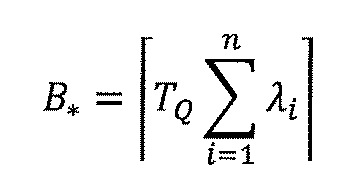
でバッファサイズが表される。ここで、nは品種数とする。
バッファサイズによる仕掛り数上限値の制御は、強制的に前の工程(この場合は洗浄工程)を停止(処理待機)させるので、スムーズな生産をする上ではあまり望ましいことではないことから、本実施形態では、あくまでカンバン方式の仕掛り数によるQ-time遵守の制御をより確実にするために用いる機能と位置付けている。
以上の手順で仕掛り数上限値を算出する。
また、複数のQ-time制約が干渉するQ-time制約区間において、生産率が最も低い後続の生産工程(以下、ボトルネック工程と呼ぶ)に律速される先行のQ-time制約では、カンバンの枚数の算定方法が異なる。ボトルネック工程より前のQ-time制約区間jのカンバン枚数Ns**(j)は、Q-time制約区間jのバッファサイズB*(j)とボトルネック工程のロードサイズの和として式(10)で表すことができる。
(カンバンの枚数Ns**(j))=(バッファサイズB*(j))+(ボトルネック工程のロードサイズL) (10)
以上の手順で仕掛り数上限値を算出する。
また、複数のQ-time制約が干渉するQ-time制約区間において、生産率が最も低い後続の生産工程(以下、ボトルネック工程と呼ぶ)に律速される先行のQ-time制約では、カンバンの枚数の算定方法が異なる。ボトルネック工程より前のQ-time制約区間jのカンバン枚数Ns**(j)は、Q-time制約区間jのバッファサイズB*(j)とボトルネック工程のロードサイズの和として式(10)で表すことができる。
(カンバンの枚数Ns**(j))=(バッファサイズB*(j))+(ボトルネック工程のロードサイズL) (10)
次に、その上限値の設定をした場合としなかった場合についてその性能を比較する。
以下、単一品種シミュレーション実験について説明する。
[目的と方法]
単一品種シミュレーション実験を行う目的は、まず単一品種において、算出したカンバン枚数、バッファサイズの設定がQ-time制約を守りつつ他の性能指標も悪化させないことを確かめるためである。
図10は、単一品種基本モデルを示す図である。図11は、単一品種基本モデル(工程)を示す図である。図12は、単一品種基本モデル(品種)を示す図である。
実験方法として、図10、図11、図12に示す通り、洗浄工程・熱処理工程のバッチ処理ライン、1品種、洗浄工程の装置台数4台、熱処理工程の装置台数5台の複数装置群を想定したシミュレーション実験を行う。洗浄工程は、バッチ・マルチタスク型の装置群で構成され、実効処理時間90分、他方の熱処理工程は、バッチ装置で構成され、実効処理時間240分のである。また、図11、図12に示す通りバッチサイズと装置台数も異なる。
以下、単一品種シミュレーション実験について説明する。
[目的と方法]
単一品種シミュレーション実験を行う目的は、まず単一品種において、算出したカンバン枚数、バッファサイズの設定がQ-time制約を守りつつ他の性能指標も悪化させないことを確かめるためである。
図10は、単一品種基本モデルを示す図である。図11は、単一品種基本モデル(工程)を示す図である。図12は、単一品種基本モデル(品種)を示す図である。
実験方法として、図10、図11、図12に示す通り、洗浄工程・熱処理工程のバッチ処理ライン、1品種、洗浄工程の装置台数4台、熱処理工程の装置台数5台の複数装置群を想定したシミュレーション実験を行う。洗浄工程は、バッチ・マルチタスク型の装置群で構成され、実効処理時間90分、他方の熱処理工程は、バッチ装置で構成され、実効処理時間240分のである。また、図11、図12に示す通りバッチサイズと装置台数も異なる。
以上のようなモデルを用いて、到着率を変化させて実験を行う。品種の到着率は洗浄、熱処理の2つの工程の処理能力の小さい方のトラフィック強度(利用率)が0.3、0.6、0.8、1.0、1.2、1.5となるように決定した。決定した到着率をもとに、定期投入、指数投入の2つの場合についてシミュレーション実験を行う。なお、本実施形態での実験ではすべて熱処理工程の方が処理能力は小さいため、到着率は熱処理工程のトラフィック強度を基準に決定されている。
これらのことを踏まえたうえで、Q-time制約を割ってしまった場合にリワークをすることを設定したモデル(QT)、QTのモデルに、算出したカンバンの枚数とバッファサイズを設定したモデル(CKB法)、そして、処理開始時点において装置状態と先行WIP数(仕掛り数)からQ-time制約が守れるかどうかを判断して製品の投入の可否を決定する従来型モデル(CT)の3つのモデルについてシミュレーション実験を行い、その性能を比較する。
また、ロットの処理順序は先入れ先出し順(First In First Out)とし、ロードルールは洗浄工程、熱処理工程ともに、ロット数がバッチサイズを満たした場合にのみ処理を開始するフルロード(Full Load)を用いる。
また、ロットの処理順序は先入れ先出し順(First In First Out)とし、ロードルールは洗浄工程、熱処理工程ともに、ロット数がバッチサイズを満たした場合にのみ処理を開始するフルロード(Full Load)を用いる。
[結果]
シミュレーション実験によって得られた結果の中から、Q-time制約割れが発生していない工場の定常状態を想定したトラフィック強度0.8の非ボトルネックの状態と、故障などによってサービス能力が低下し、一時的に到着率がサービス能力を上回ったためにQ-time制約割れが発生しやすい状況とを想定したトラフィック強度1.2のボトルネックの状態の結果を以下に示す。
図13は、評価比較(単一品種、定期投入、非ボトルネック、ρ=0.8)を示す図である。図14は、評価比較(単一品種、定期投入、ボトルネック、ρ=1.2)を示す図である。図15は、評価比較(単一品種、指数投入、非ボトルネック、ρ=0.8)を示す図である。図16は、評価比較(単一品種、指数投入、ボトルネック、ρ=1.2)を示す図である。
図13と図14が定期投入の場合の結果を表し、図15、図16が指数投入の場合の結果を表す。ここでは、性能が良かったものをアンダーラインで、性能が悪かったものを太字で示している。
シミュレーション実験によって得られた結果の中から、Q-time制約割れが発生していない工場の定常状態を想定したトラフィック強度0.8の非ボトルネックの状態と、故障などによってサービス能力が低下し、一時的に到着率がサービス能力を上回ったためにQ-time制約割れが発生しやすい状況とを想定したトラフィック強度1.2のボトルネックの状態の結果を以下に示す。
図13は、評価比較(単一品種、定期投入、非ボトルネック、ρ=0.8)を示す図である。図14は、評価比較(単一品種、定期投入、ボトルネック、ρ=1.2)を示す図である。図15は、評価比較(単一品種、指数投入、非ボトルネック、ρ=0.8)を示す図である。図16は、評価比較(単一品種、指数投入、ボトルネック、ρ=1.2)を示す図である。
図13と図14が定期投入の場合の結果を表し、図15、図16が指数投入の場合の結果を表す。ここでは、性能が良かったものをアンダーラインで、性能が悪かったものを太字で示している。
[考察]
以上の実験結果から、定期投入・指数投入どちらの場合であっても、トラフィック強度0.8の非ボトルネックの状態においては、カンバンの枚数とバッファサイズを設定しても、性能が低下していないことが見て取れる。また、この状態ではどの機能においてもリワークが発生していないため、Q-time制約割れが起こっていないことがわかる。トラフィック強度1.2のボトルネックの状態においてはQTのモデルでは定期投入・指数投入にかかわらず多数のQ-time制約割れが起こっているが、CKB法、CTのモデルではリワークがゼロに抑えられている。
以上の実験結果から、定期投入・指数投入どちらの場合であっても、トラフィック強度0.8の非ボトルネックの状態においては、カンバンの枚数とバッファサイズを設定しても、性能が低下していないことが見て取れる。また、この状態ではどの機能においてもリワークが発生していないため、Q-time制約割れが起こっていないことがわかる。トラフィック強度1.2のボトルネックの状態においてはQTのモデルでは定期投入・指数投入にかかわらず多数のQ-time制約割れが起こっているが、CKB法、CTのモデルではリワークがゼロに抑えられている。
サイクルタイムはCKB法、CTのモデルの値が大きいが、これは出力されたロットが洗浄工程の前で意図的に待機させられた結果と考えられる。しかし、結果としてスループットは低下していないので必ずしも性能が悪化したとはいえない。稼働率に関しては、CKB法、CTのモデル、ともにQTのモデルよりも低い稼働率で同じ量のスループットを実現できているので、コスト面の性能はむしろ良くなっている。
単一品種における実験では、カンバンとバッファサイズで大きく性能を落とさずQ-time制約割れを防ぐことができたが、現段階では必ずしもそれが最善の方法とは言えない。複数品種が混在する場合においても実験を行い、その性能を比較していく。
単一品種における実験では、カンバンとバッファサイズで大きく性能を落とさずQ-time制約割れを防ぐことができたが、現段階では必ずしもそれが最善の方法とは言えない。複数品種が混在する場合においても実験を行い、その性能を比較していく。
以下、複数品種シミュレーション実験について説明する。
[目的と方法]
複数品種シミュレーション実験を行う目的は、単一品種で行った実験が、複数の品種が混在し、装置を共有している場合でも同様の目的が達成できていることを確かめるためである。なお、この実験のモデルは実際の工場で使われている洗浄工程・熱処理工程のバッチ処理の連続工程である。
図17は、複数品種基本モデルを示す図である。図18は、複数品種基本モデル(工程)を示す図である。図19は、複数品種基本モデル(品種)を示す図である。図20は、処理可能装置(洗浄)を示す図である。図21は、処理可能装置(熱処理)を示す図である。
実験方法として、図17、図18、図19に示す通り、単一品種の場合と同様、洗浄工程・熱処理工程のバッチ処理の連続工程、3品種、洗浄工程・装置台数5台、熱処理工程・装置台数6台の複数装置群を想定したシミュレーション実験を行う。
[目的と方法]
複数品種シミュレーション実験を行う目的は、単一品種で行った実験が、複数の品種が混在し、装置を共有している場合でも同様の目的が達成できていることを確かめるためである。なお、この実験のモデルは実際の工場で使われている洗浄工程・熱処理工程のバッチ処理の連続工程である。
図17は、複数品種基本モデルを示す図である。図18は、複数品種基本モデル(工程)を示す図である。図19は、複数品種基本モデル(品種)を示す図である。図20は、処理可能装置(洗浄)を示す図である。図21は、処理可能装置(熱処理)を示す図である。
実験方法として、図17、図18、図19に示す通り、単一品種の場合と同様、洗浄工程・熱処理工程のバッチ処理の連続工程、3品種、洗浄工程・装置台数5台、熱処理工程・装置台数6台の複数装置群を想定したシミュレーション実験を行う。
洗浄工程は、バッチシーケンシャル型の装置群で構成され、他方の熱処理工程は、バッチ装置で構成され、図20、図21のようにバッチサイズと装置台数も異なる。実効処理時間、使用装置台数は品種ごとに異なり、品種1(p1)は洗浄工程の実効処理時間90分、使用装置台数5台、熱処理工程の実効処理時間242分、使用装置台数4台である。品種2(p2)は洗浄工程の実効処理時間90分、使用装置台数4台、熱処理工程の実効処理時間240分、使用装置台数5台である。品種3(p3)は洗浄工程の実効処理時間90分、使用装置台数5台、熱処理工程の実効処理時間195分、使用装置台数5台である。また、品種はそれぞれ処理できる装置が決められている。洗浄工程では、図20に表すように、p1、p2、p3のそれぞれ使用する装置が異なる。熱処理工程でも、図21に表すように、p1、p2、p3の品種の別で使用する装置が異なるものがある。
以上のようなモデルを用いて、到着率を変化させて実験を行う。品種の到着率は前節の実験と同様に、洗浄、熱処理の2つの工程の処理能力の小さい方のトラフィック強度(利用率)が0.3、0.6、0.8、1.0、1.2、1.5となるように決定する。本実施形態では、すべて熱処理工程の方が処理能力が小さいため、トラフィック強度(ρ:利用率)はすべて熱処理工程のものを用いる。
しかし、複数の品種が混在する場合は品種ごとに、実効処理時間・使用できる装置台数が異なるため、それぞれ別々に到着率を求める必要がある。図15に示すように、品種の到着率は前もってトラフィック強度を決めて品種ごとに処理能力(μ:(μ=LTp/L:ロードサイズTp:処理時間))、使用装置台数(m)から逆算をして決定する。到着率を決める際の前提として、装置が複数の品種を処理する場合、それらを均等の割合で処理をすることを仮定した。
しかし、複数の品種が混在する場合は品種ごとに、実効処理時間・使用できる装置台数が異なるため、それぞれ別々に到着率を求める必要がある。図15に示すように、品種の到着率は前もってトラフィック強度を決めて品種ごとに処理能力(μ:(μ=LTp/L:ロードサイズTp:処理時間))、使用装置台数(m)から逆算をして決定する。到着率を決める際の前提として、装置が複数の品種を処理する場合、それらを均等の割合で処理をすることを仮定した。
以下に投入率決定の手順を示す。なお、図22は、投入率の決定について説明するための図である。
(1)ρ>1の場合、ρを1として計算を行う
(2)各共用装置における各品種の生産比率から、各品種の投入率を計算
(3)品種ごとに、全ての装置における投入率を足し合わせる
(4)足し合わせた投入率から、品種の投入率を算定する
これらのことを踏まえたうえで、先ほどと同様のQT、CTのモデル、品種ごとにカンバン枚数を設定し、バッファサイズを設けたCKB法のモデル、品種ごとの差別を設けず工程全体でカンバン枚数を設定し、バッファサイズを設けたCKB-法のモデルの4つのモデルにおいて実験をし、その性能を比較する。
(1)ρ>1の場合、ρを1として計算を行う
(2)各共用装置における各品種の生産比率から、各品種の投入率を計算
(3)品種ごとに、全ての装置における投入率を足し合わせる
(4)足し合わせた投入率から、品種の投入率を算定する
これらのことを踏まえたうえで、先ほどと同様のQT、CTのモデル、品種ごとにカンバン枚数を設定し、バッファサイズを設けたCKB法のモデル、品種ごとの差別を設けず工程全体でカンバン枚数を設定し、バッファサイズを設けたCKB-法のモデルの4つのモデルにおいて実験をし、その性能を比較する。
[結果]
図23は、評価比較(複数品種、指数投入、非ボトルネック、ρ=0.8)を示す図である。図24は、評価比較(複数品種、指数投入、ボトルネック、ρ=1.2)を示す図である。
まず、トラフィック強度が0.8、1.2の両方の場合において、CKB法がQ-time制約割れを抑制している。
複数品種が混在しているモデルにおける実験では、指数投入の場合トラフィック強度が0.3、0.6の場合に、全てのモデルにおいてQ-time制約割れが発生していた。
図23は、評価比較(複数品種、指数投入、非ボトルネック、ρ=0.8)を示す図である。図24は、評価比較(複数品種、指数投入、ボトルネック、ρ=1.2)を示す図である。
まず、トラフィック強度が0.8、1.2の両方の場合において、CKB法がQ-time制約割れを抑制している。
複数品種が混在しているモデルにおける実験では、指数投入の場合トラフィック強度が0.3、0.6の場合に、全てのモデルにおいてQ-time制約割れが発生していた。
そこで、前節と同様のQ-time制約割れが発生していないトラフィック強度0.8の非ボトルネックの状態と、Q-time制約割れが発生しているトラフィック強度1.2のボトルネックの状態の結果に加えて、指数投入の場合において、トラフィック強度0.3の実験結果も示す。ただし、複数品種の場合、品種によって投入数が異なるため、すべての品種の処理が均等に行われているか否かを検証する指標を追加する。処理数に偏りが生じると納期に悪影響を与えることが考えられる。よって、品種ごとにスループットが異なる場合については、各品種の投入率に対するスループット(出力率)の割合を新たに指標として設けることとした。また、リワークが起こったモデルに関してはリワークを投入に加えた第1工程全体の投入に対するスループットの割合を性能評価指標としている。図23、図24が指数投入の場合の結果を表す。
[考察]
定期投入でトラフィック強度0.8の非ボトルネックの状態のときはCT、CKB法、CKB-法において1%稼働当たりのスループットが高くなっており、平均仕掛りも低く抑えられている。どれもリワークが起きておらず、性能の悪化も見られない。ここで、サイクルタイムと仕掛りは片方が小さくなれば、もう一方も小さくなる対応関係にあるはずなのにもかかわらず、その挙動が結果からみられないのは、その差が小数点第二位以下のためである。トラフィック強度1.2(ボトルネックの状態)では、図27の通りQTに比べてCT、CKB法、およびCKB-法でQ-time制約割れを大幅に抑えられている。特に、CKB法では、Q-time割れをゼロに抑え、基準となるQTに比べてリワークを完全抑制しつつ、スループットを高く、平均サイクルタイムは短く、仕掛数も少なくなる性能改善を果たしている。
定期投入でトラフィック強度0.8の非ボトルネックの状態のときはCT、CKB法、CKB-法において1%稼働当たりのスループットが高くなっており、平均仕掛りも低く抑えられている。どれもリワークが起きておらず、性能の悪化も見られない。ここで、サイクルタイムと仕掛りは片方が小さくなれば、もう一方も小さくなる対応関係にあるはずなのにもかかわらず、その挙動が結果からみられないのは、その差が小数点第二位以下のためである。トラフィック強度1.2(ボトルネックの状態)では、図27の通りQTに比べてCT、CKB法、およびCKB-法でQ-time制約割れを大幅に抑えられている。特に、CKB法では、Q-time割れをゼロに抑え、基準となるQTに比べてリワークを完全抑制しつつ、スループットを高く、平均サイクルタイムは短く、仕掛数も少なくなる性能改善を果たしている。
一方、従来法のCTルールでは、QTルールよりは少ないもののQ-time制約割れが発生し、また、各品種をバランスよく処理できない等の副作用が出る(図24青字部分)。また、品種別に管理しない設定を施したCKB-法では、各品種をバランスよく処理するが、リワーク数などの性能は芳しくなく、CKB法の品種別カンバン数の管理が有効であることがわかる。これらのシミュレーション結果は、賞味40日間(シミュレーション期間50日)のデータによる性能評価結果であり、期間長に比例してルールによる差は更に広がる。
基本となるQTのモデルは洗浄工程の1%稼働当たりのスループットは高くなっているが、熱処理工程のそれは低下している。これはボトルネックであるはずの熱処理工程を十分に稼働しきれていないことが原因と考えられ、工場全体から考えれば性能が悪化しているといえる。何より、リワークが多く(32%)発生していることが性能としてよくない。CT、CKB法、CKB-法はQTに比べ平均仕掛りに関しては性能の悪化は見られない。最終仕掛りの差はスループットの差がロット換算されて表されている。この差は品種の不均等な処理が生んだ結果と考えられる。
指数投入について、トラフィック強度0.3の非ボトルネックの状態の特徴として、どのモデルでもリワークが発生していることが挙げられる。この原因は後に詳しく分析していくことにする。トラフィック強度0.8の非ボトルネックの状態では、CT、CKB法、CKB-法のどれもQTと比べると性能の悪化は見られず、品種ごとのサイクルタイム、平均仕掛りにばらつきがあるとしても、全体平均は悪化していない。トラフィック強度1.2のボトルネックの状態では、リワークを完全に抑えられているのはCKB法のみで、CTも到着がばらついたりするとQ-time制約遵守にも限界が生じることが明らかになった。
リワークを含めた処理の割合はCT、QTよりもCKB法、CKB-法がともに高く、全体スループットはCT、CKB法、CKB-法のどれもQTよりも高い値を示している。1%稼働当たりのスループットもどれもQTよりも悪化していない。サイクルタイム、平均仕掛りは品種ごとにばらつきはあるにしても全体平均はQTより悪化していないことが見て取れる。
リトルの方式用いて算出した最大待ちロット数、仕掛り数を品種ごとにカンバン枚数を設定し、バッファサイズを設けたCKB法のモデルが極端にWIPの到着が少ない場合を除いて完全にQ-time制約割れを抑えることができ、かつ品種の処理が均等に行われ、性能が悪化しない、性能指標によっては改善もされていることが確認できた。Q-time割れが起こりやすい(ρ=1.2)場合において、CKB法を適用しない場合に約32%であるリワーク率(Q-time制約割れ率)を確実にゼロに抑えて製品品質の劣化を防ぎ、かつ、スループット、平均サイクルタイム、仕掛在庫等も改善でき、従来法より優れた生産率(=(生産量)/(投入量))を達成する結果を得た。
以上の実験結果から、極端にWIPの到着が少ない場合を除けば品種ごとに仕掛り数上限値を設定するCKB法の性能が最も良いことが明らかになった。
以上の実験結果から、極端にWIPの到着が少ない場合を除けば品種ごとに仕掛り数上限値を設定するCKB法の性能が最も良いことが明らかになった。
以下、CKB法のモデルを基に考えていくこととする。
ここからは、前述した指数投入でトラフィック強度が0.3のときに発生しているリワークについて考察する。この場合のリワーク発生は、本実施形態の仕掛り数上限値の制御とは直接関係がない。そこで別のアプローチによって問題を解決していく。
まず、トラフィック強度0.3のときにリワークが発生する理由について、ロットの到着が遅いため、Q-time制約の時間以内にバッチが組めず(バッチサイズ分のロットが到着せず)、処理開始ができないためだと考えられる。
ここからは、前述した指数投入でトラフィック強度が0.3のときに発生しているリワークについて考察する。この場合のリワーク発生は、本実施形態の仕掛り数上限値の制御とは直接関係がない。そこで別のアプローチによって問題を解決していく。
まず、トラフィック強度0.3のときにリワークが発生する理由について、ロットの到着が遅いため、Q-time制約の時間以内にバッチが組めず(バッチサイズ分のロットが到着せず)、処理開始ができないためだと考えられる。
複数品種のトラフィック強度0.3のQTのモデルにおいて「Q-time制約の時間を超えたらリワークをする」という条件をなくして実験し、その時のロットの工程間滞在時間を表したヒストグラムが図25である。この図から確かにQ-time制約割れとなる、滞在時間が720分(12時間)を超えるロットが存在していることがわかる。Q-time制約割れを起こしていたロットは、品種1と品種2のみであった。これらのロットのQ-time制約割れの原因を探るため、Q-time制約割れを起こしているロットと、そのロットとバッチ組をしたロットを抜き出し、その中から2つを図26に示した。この表から、定期投入であれば、Q-time制約割れが起きる前にバッチを組むことができ、ロットが処理を開始できるはずにもかかわらず、指数投入によってロットの到着にばらつきが生じ、ロットの到着が遅れ、バッチ組時間が長くなった結果としてQ-time制約割れが起こっていることが見て取れる。
図25は、ρ=0.3におけるリワーク状況を示す図である。図26は、ρ=0.3におけるリワーク要因を示す図である。図27は、ルール比較(複数品種、指数投入、非ボトルネック、ρ=0.3)を示す図である。図28は、ルール比較(複数品種、指数投入、非ボトルネック、ρ=0.8を示す図である。図29は、ルール比較(複数品種、指数投入、ボトルネック、ρ=1.2)を示す図である。
このようなロットの到着が少ない状況で、到着のばらつきによって生じてしまうQ-time制約割れを防ぐために、ロードルールを変えて実験を行う。各ロードルールの説明は図7に示す。これまでの実験では、ロードルールはすべてフルロードで行ってきた。
このようなロットの到着が少ない状況で、到着のばらつきによって生じてしまうQ-time制約割れを防ぐために、ロードルールを変えて実験を行う。各ロードルールの説明は図7に示す。これまでの実験では、ロードルールはすべてフルロードで行ってきた。
しかし、これでは先ほどのようにバッチ組を待つことによってQ-time制約割れを起こしてしまう。そこで熱処理工程のロードルールのみを変化させて実験を行う。比較するモデルは熱処理工程のロードルールがFull、PLA、そしてAFLの3つのモデルを比較する。また、トラフィック強度が0.3のときは、Fullにおけるp1のカンバン枚数が熱処理工程のバッチサイズ6ロットよりも小さい4枚になった。そこで、p1のみを4ロットで処理をする設定にしたモデル(p1Full4)でも同様の実験を行った。ただし、トラフィック強度が0.6以上になったときはp1Full4のモデルはカンバン枚数が6枚を超え、すべてFullと同様の設定、結果になる。実験はこれまでと同様、熱処理工程のトラフィック強度を基準に到着率を決定して行った。結果はその中からトラフィック強度0.3、0.8、1.2の場合のものを抜き出して図27、図28、図29に示す。
以上の実験結果からトラフィック強度が0.3のときは第2工程(熱処理)のロードルールがPLA、AFLの場合にはリワークも抑えられ、かつ、スループット、サイクルタイムなど他の性能評価指標も良いことが読み取れる。p1Full4ではリワークが完全に抑えられていない。これは理論的なカンバン枚数の設定で処理することが可能であれば、必ずしもQ-time制約割れを抑えることができるわけではないことを示している。しかし、ロードサイズを小さくすることによって中性的な評価が得られることは明らかになった。
よって、WIPの到着が遅い場合には、カンバン枚数だけではリワークは制御できず、ロードルールの変更によってリワークを制御するほうが良いことがわかった。トラフィック強度が0.8の場合はFullの方がスループット、サイクルタイムなどの性能評価指標が良い値を示している。トラフィック強度が1.2の場合においては、すべて性能は同じという結果になった。
以上より、トラフィック強度が0.3の場合でもPLA、AFLのロードルールを用いればQ-time制約割れを起こさず、かつ性能評価指標も悪化しないことが明らかになった。しかし、トラフィック強度が0.8の場合はFullのロードルールの方が性能は良いことからより良い生産スケジューリングを行うためには、工程の状態を監視し、トラフィック強度の変化によってロードルールを変化させる必要があると考えられる。
以上より、トラフィック強度が0.3の場合でもPLA、AFLのロードルールを用いればQ-time制約割れを起こさず、かつ性能評価指標も悪化しないことが明らかになった。しかし、トラフィック強度が0.8の場合はFullのロードルールの方が性能は良いことからより良い生産スケジューリングを行うためには、工程の状態を監視し、トラフィック強度の変化によってロードルールを変化させる必要があると考えられる。
[結論]
本実施形態では、半導体製造において重要性の高いQ-time制約に焦点を当て、特に重要性が指摘されている洗浄・熱処理工程のバッチ処理の連続工程のQ-time制約区間を取り上げた。現在までのQ-time制約に関する先行技術では厳密性・精度が不十分で、Q-time制約遵守以外の他の性能指標に対する影響が考慮されていなかった。本実施形態では、Q-time制約を守りつつ、他の性能指標も極力悪化させない生産スケジューリング手法として、Q-time制約区間の仕掛り数の上限値を制御するCKB法を構築し、その性能を確率的シミュレーション実験により評価した。CKB法は、カンバン方式と待ち行列理論を基礎として理論的にカンバン枚数や仕掛数上限値を計算するため信頼性と汎用性が高い。また、特に通常の工場で多い工程利用率60%以上の状況で特に効果を発揮することが確かめられた。
本実施形態では、半導体製造において重要性の高いQ-time制約に焦点を当て、特に重要性が指摘されている洗浄・熱処理工程のバッチ処理の連続工程のQ-time制約区間を取り上げた。現在までのQ-time制約に関する先行技術では厳密性・精度が不十分で、Q-time制約遵守以外の他の性能指標に対する影響が考慮されていなかった。本実施形態では、Q-time制約を守りつつ、他の性能指標も極力悪化させない生産スケジューリング手法として、Q-time制約区間の仕掛り数の上限値を制御するCKB法を構築し、その性能を確率的シミュレーション実験により評価した。CKB法は、カンバン方式と待ち行列理論を基礎として理論的にカンバン枚数や仕掛数上限値を計算するため信頼性と汎用性が高い。また、特に通常の工場で多い工程利用率60%以上の状況で特に効果を発揮することが確かめられた。
本実施形態では、Q-time制約割れの原因になる2つ目の原因である到着率が低い状況(トラフィック強度0.3の場合など)に対しても、ロードルール等の簡単な変更で確実にQ-timeを遵守する対処方法を考え、シミュレーション結果からQ-time割れを防ぐことを確認した。本実施形態では、到着率が低くても、バッチ型やバッチ・マルチタスク型装置では、ロードルールなどの設定などによってQ-time制約割れが起こる場合がある。この場合を判断して、以下のように適切にロードルールを変えることで、Q-time制約割れを回避しつつ、生産性を高めることができる(CKB法と合わせて利用する)。最適ロードルール判定部19は、到着のばらつきを考慮したバッチ組待ち時間TBとQ-time制約(上限)T_(Q+)の大小関係が切り替わるTB≦T_(Q+)なる到着率λ≧Lの境界値Lを算定しておき、適切なロードルールを使う。λ≧Lの場合は、Full load(フルサイズのバッチ組を強制)。λ<Lの場合は、PLAやAFLなど、フルサイズのバッチ組を強制しない方法を使う。本実施形態は、到着率が低くばらつきがある場合以外にも、製品品種や工程によって到着率の大小が違うため考慮しておく。
また、装置の故障やメンテナンスが発生し、装置の処理能力が変動することがある。それらの状況を考慮した場合でも、本実施形態で用いたカンバン枚数やバッファサイズの決定は、到着率や処理能力の変動に対して、高速かつ高い精度で計算が可能で、しかも確実にQ-time制約割れを防ぐことができる。
以上のようにQ-time制約を守りつつ他の性能指標も悪化させない生産スケジューリング手法として、計算スピード、精度、実用性などの定性的評価も高いCKB法の構築と性能評価と通して目的を達成することができた。
以上のようにQ-time制約を守りつつ他の性能指標も悪化させない生産スケジューリング手法として、計算スピード、精度、実用性などの定性的評価も高いCKB法の構築と性能評価と通して目的を達成することができた。
第1実施形態では、CKB法により第1問題点を解決している。
多品種生産において、Q-time制約を遵守しつつ高いスループットを達成する実用的な生産物流管理方法を、CKB(Control of Kanban and Buffer sizes)法と名付けた。第1実施形態では、CKB法のプログラムとそれを用いた性能評価結果(実際の工場のデータを用いた確率的シミュレーションによる)である。この性能評価結果から、CKB法を適用しない場合に約32%であるリワーク率(Q-time制約割れ率)を確実にゼロに抑えて製品品質の劣化を防ぎ、かつ、スループット、平均サイクルタイム、仕掛在庫等も改善でき、従来法より優れた生産率(=生産量/投入量)を達成する結果を得ている。
多品種生産において、Q-time制約を遵守しつつ高いスループットを達成する実用的な生産物流管理方法を、CKB(Control of Kanban and Buffer sizes)法と名付けた。第1実施形態では、CKB法のプログラムとそれを用いた性能評価結果(実際の工場のデータを用いた確率的シミュレーションによる)である。この性能評価結果から、CKB法を適用しない場合に約32%であるリワーク率(Q-time制約割れ率)を確実にゼロに抑えて製品品質の劣化を防ぎ、かつ、スループット、平均サイクルタイム、仕掛在庫等も改善でき、従来法より優れた生産率(=生産量/投入量)を達成する結果を得ている。
<第2実施形態>
図30を参照して、本発明の第2実施形態に係る最適指標生成装置について説明する。 本発明の第2実施形態に係る最適指標生成装置21は、例えば、製造装置の予防保全時期を分散化する運用方法について、生産工程#1にそれぞれ設けられた装置群5の保全スケジュールを管理する生産管理システム10およびエンジニアリング業務システム29を制御の対象としている。本実施形態では、保全時期分散化のための生産負荷配分方法(以下、JAMP法という)について説明する。
図30を参照して、本発明の第2実施形態に係る最適指標生成装置について説明する。 本発明の第2実施形態に係る最適指標生成装置21は、例えば、製造装置の予防保全時期を分散化する運用方法について、生産工程#1にそれぞれ設けられた装置群5の保全スケジュールを管理する生産管理システム10およびエンジニアリング業務システム29を制御の対象としている。本実施形態では、保全時期分散化のための生産負荷配分方法(以下、JAMP法という)について説明する。
図30に示すように、最適指標生成装置21は、入力部22、補助入力部23、装置区分算定部28、JAMP最適論理値計算部24、感度解析部(JAMP特性)25、開始終了時期算出部26、感度解析部(性能特性)27を備えている。
入力部22は、生産管理システム10やエンジニアリング業務システム29からメンテナンス時間、メンテナンス指針(定量メンテナンスでは、メンテナンス開始までの処理数、定期メンテナンスではメンテナンス周期など)、装置群(工程)の装置台数、装置群(工程)の製品品種別生産数量または到着率、品種・工程/装置別の処理時間、装置で処理可能な品種情報、装置種別を入力する。
入力部22は、生産管理システム10やエンジニアリング業務システム29からメンテナンス時間、メンテナンス指針(定量メンテナンスでは、メンテナンス開始までの処理数、定期メンテナンスではメンテナンス周期など)、装置群(工程)の装置台数、装置群(工程)の製品品種別生産数量または到着率、品種・工程/装置別の処理時間、装置で処理可能な品種情報、装置種別を入力する。
補助入力部23は、生産管理システム10やエンジニアリング業務システム29から段取り時間、バッチ型装置に関する情報(バッチサイズ、ロードルール、ロードサイズ、ロード間隔)、マルチタスク型装置に関する情報(装置内の待機箇所の有無と容量値など)、入力部からも得られる情報(装置種別、装置台数、処理時間、装置群(工程)の品種別生産数量または到着率、装置で処理可能な品種情報)の全てを入力する。補助入力部23は、必須ではない入力データを入力するが、実用上、次段階のJAMP最適論理値計算部24で重要となるデータをまとめて前処理を行い、段取り時間(製品品種・装置・工程別)、バッチ装置に関する情報(平均ロードサイズ、ロード間隔、バッチ組時間、装置の実行サービス率)、MTBF(平均故障間隔)、MTTR(平均修繕時間)、マルチタスク型装置に関する情報(装置の待機の有無と容量値)などを出力する。なお、この補助入力部23からデータが入力された場合には、JAMP法最適理論値計算部24においてより詳細な計算を行う。
JAMP最適論理値計算部24は、入力されるメンテナンス時間、メンテナンス指針、装置台数、製品品種別生産数量または到着率、品種・工程/装置別の処理時間、装置で処理可能な品種情報、装置種別、段取り時間、その他装置に関する情報に基づいて、JAMP法理論値計算結果、各装置の処理負荷(回数)とその処理時期を算出して出力する。
感度解析部(JAMP特性)25は、JAMP最適論理値計算部24から入力されるJAMP法理論値計算結果、各装置の処理負荷(回数)とその処理時期が変動した場合のJAMP法理論値計算の結果の変化特性を算定する。感度解析部(JAMP特性)25は、この感度解析結果を、内部記憶部25aに記録しておき、JAMP法理論値計算結果、各装置の処理負荷(回数)とその処理時期が動的に変化した場合に、即時に更新データとして使用することもできる。
感度解析部(JAMP特性)25は、JAMP最適論理値計算部24から入力されるJAMP法理論値計算結果、各装置の処理負荷(回数)とその処理時期が変動した場合のJAMP法理論値計算の結果の変化特性を算定する。感度解析部(JAMP特性)25は、この感度解析結果を、内部記憶部25aに記録しておき、JAMP法理論値計算結果、各装置の処理負荷(回数)とその処理時期が動的に変化した場合に、即時に更新データとして使用することもできる。
開始終了時期算出部26は、処理予定のロット情報やエンジニアリング情報を入力し、JAMP法理論値計算結果から、各装置の処理および予防保全の開始・終了時期を算定する。そして、予防保全スケジュールとして、常用装置および代替装置のそれぞれの処理および予防保全の開始・終了時刻を出力する。
感度解析部(性能特性)27は、JAMP法に使用した入力データ、JAMP法最適理論値の条件を入力し、決定されたJAMP法最適理論値の条件の下で、工程の性能評価のための計算を行い、性能特性として、トラフィック強度v.s.各種性能評価指標を生産管理システム10に出力する。
感度解析部(性能特性)27は、JAMP法に使用した入力データ、JAMP法最適理論値の条件を入力し、決定されたJAMP法最適理論値の条件の下で、工程の性能評価のための計算を行い、性能特性として、トラフィック強度v.s.各種性能評価指標を生産管理システム10に出力する。
装置区分算定部28は、入力部22と補助入力部23とから入力される情報に基づいて、装置を常用装置と代替装置(常用能力と代替能力)に区分し、装置区分情報を出力する。常用装置(常用能力)は、ロットの待ちが長大化しないために定常的に必要な装置能力を指し、代替装置(代替能力)はそれ以外の平均的な余剰能力を指す。装置群に含まれる装置台数をm、各装置のサービス率の加重平均をμとすると、装置群(工程)のサービス能力はM=mμとなる。ここで、当該装置群製品の投入率をΛとするとき、常用能力は、Λ/μで、常用装置は、

台となる。この時、代替能力は(m-Λ/μ)で、代替装置は、
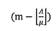
台となる。
台となる。この時、代替能力は(m-Λ/μ)で、代替装置は、
台となる。
エンジニアリング業務システム29は、主に生産設備の予防保全や故障対応等の業務を管理とりまとめるシステムで、生産管理システム10において保持していない、エンジニアリング業務全般の条件や予定・実績を管理する。例えば、装置エンジニアの担当範囲などのマスター情報、シフトなどの実行条件、予防保全や故障対応の実績データなどである。生産管理システムによっては、エンジニアリング業務システム29が、生産管理システム10の機能として組み込まれている場合もある。
図30を参照して、本発明の第2実施形態に係る最適指標生成装置31の動作について説明する。
生産実行システムに含まれる複数の装置に関する情報を生産管理システム10を介して入力部22により入力し、また、装置区分算定部28により複数の装置を常用能力を有する常用装置と代替能力を有する代替装置とに区分し、装置能力区分と入力された情報から複数の常用装置と代替装置(および常用能力と代替能力)の稼働回数と稼働時期を算出するとともに、常用装置と代替装置とに関する予防保全開始・終了時期を開始終了時期算出部26により算出し、開始終了時期算出部26により算出された最適な開始終了時期情報を生産管理システム10やエンジニアリング業務システム29に供給する。
生産実行システムに含まれる複数の装置に関する情報を生産管理システム10を介して入力部22により入力し、また、装置区分算定部28により複数の装置を常用能力を有する常用装置と代替能力を有する代替装置とに区分し、装置能力区分と入力された情報から複数の常用装置と代替装置(および常用能力と代替能力)の稼働回数と稼働時期を算出するとともに、常用装置と代替装置とに関する予防保全開始・終了時期を開始終了時期算出部26により算出し、開始終了時期算出部26により算出された最適な開始終了時期情報を生産管理システム10やエンジニアリング業務システム29に供給する。
これにより、従来法では達成されていなかったQ-time制約割れの主要な原因である、装置の予防保全に対しても、解析方法と適正な管理手法を与えることで、Q-time制約遵守しつつ良品スループットの向上とコスト低減・環境負荷低減を同時に達成することができる。これにより、Q-time制約割れが起こりやすい状況を軽減し、Q-time制約を確実に遵守しつつ、良品スループット向上とコスト低減および環境負荷低減を達成することが可能な最適オペレーション管理条件を提供することができる。
以下、本発明の第2実施形態に係る最適指標生成装置21を構成する各部の動作について説明する。
まず、最適指標生成装置21による製造装置の予防保全時期を分散化する運用方法について説明する。
[生産設備管理の重要性]
半導体製造において、製造コストの4割~6.5割は機械設備の減価償却であり、重要な管理対象である。一般に、化学物理的な処理を施す生産設備では、故障や異常状態に陥った場合に、半製品をスクラップまたは再生処理(リワークと呼ぶ)する必要があり、これらスクラップやリワークは時間とコストの浪費になる。
また、設備状態が故障や異常になった後に正常に復帰させるための事後保全に費やす時間に比べて、故障や異常が起こらないうちに設備の保全を行った方が結果的に設備の動作時間を長くすることが可能になるため、予防保全(Preventive maintenance:PMと呼ばれる)が行われている。
予防保全には、一定時間ごとに所定のメンテナンスを行う定期メンテナンスが行われることが多いが、化学物理的な処理を行う装置に対しては、処理した回数に応じてメンテナンスを行う定量メンテナンスが行われる場合が多い。本実施形態では、半導体工場の定量メンテナンスを主に取り上げる(なお、定期メンテナンスにも適用可能である)。
まず、最適指標生成装置21による製造装置の予防保全時期を分散化する運用方法について説明する。
[生産設備管理の重要性]
半導体製造において、製造コストの4割~6.5割は機械設備の減価償却であり、重要な管理対象である。一般に、化学物理的な処理を施す生産設備では、故障や異常状態に陥った場合に、半製品をスクラップまたは再生処理(リワークと呼ぶ)する必要があり、これらスクラップやリワークは時間とコストの浪費になる。
また、設備状態が故障や異常になった後に正常に復帰させるための事後保全に費やす時間に比べて、故障や異常が起こらないうちに設備の保全を行った方が結果的に設備の動作時間を長くすることが可能になるため、予防保全(Preventive maintenance:PMと呼ばれる)が行われている。
予防保全には、一定時間ごとに所定のメンテナンスを行う定期メンテナンスが行われることが多いが、化学物理的な処理を行う装置に対しては、処理した回数に応じてメンテナンスを行う定量メンテナンスが行われる場合が多い。本実施形態では、半導体工場の定量メンテナンスを主に取り上げる(なお、定期メンテナンスにも適用可能である)。
[工場内トラフィックと予防保全の関係]
予防保全の期間(Mean Time to Repair:MTTRと呼ばれる)は、生産設備は停止し、仕掛品(Work-in-process:WIP)を処理することができない。そのため、MTTRの間は、その他の生産設備を使用して、WIPを処理していく必要がある。通常、工場内物流の混雑の程度(トラフィック)は、定常的可動状態における平均として工程利用率(トラフィック強度)を100%(1)未満として計画される。ここで、工程を実際に運用する際に、同時期にPMになる装置台数が多いと、残りの可動装置だけではWIPを処理しきれずに工程利用率が100%を超える。この状況になった場合、WIPの待ち時間が急激に長大化することが知られている。待ち時間の長大化は、コスト増加、納期遵守率やQ-time制約遵守に負の影響を及ぼす。
そのため、複数の装置のPMができるだけ同時期に発生しないよう分散化することが望まれる。
予防保全の期間(Mean Time to Repair:MTTRと呼ばれる)は、生産設備は停止し、仕掛品(Work-in-process:WIP)を処理することができない。そのため、MTTRの間は、その他の生産設備を使用して、WIPを処理していく必要がある。通常、工場内物流の混雑の程度(トラフィック)は、定常的可動状態における平均として工程利用率(トラフィック強度)を100%(1)未満として計画される。ここで、工程を実際に運用する際に、同時期にPMになる装置台数が多いと、残りの可動装置だけではWIPを処理しきれずに工程利用率が100%を超える。この状況になった場合、WIPの待ち時間が急激に長大化することが知られている。待ち時間の長大化は、コスト増加、納期遵守率やQ-time制約遵守に負の影響を及ぼす。
そのため、複数の装置のPMができるだけ同時期に発生しないよう分散化することが望まれる。
[予防保全が品質とコストに与える影響]
半導体の加工寸法は技術ロードマップに従い、微細化が進んでいる。現在、その加工寸法は髪の毛の太さの1000分の1の太さにまで小さくなってきている。これは、半導体の加工寸法を2分の1の大きさにすると、速度が2倍、消費電力が4分の1になるなど、半導体は微細化をするだけで、高性能・低コストが実現できるからである。しかし、このような加工寸法の微細化は、製造面において歩留り(良品率)の確保を困難にした。設計通りのサイズ、機能を持った製品(良品)を生産するために、加工時間と同様に工程間の滞在時間も厳密に管理しなければならなくなったのである。そのため、Q-time制約(加工と加工の間の滞在時間の上限値と下限値)を考慮した生産スケジューリングが重要になっている。本実施形態1で述べた通り、製造装置の予防保全(PM)によって待ち時間が長大化する状況では、Q-time制約割れが起こりやすくなるため、装置PMの分散化は品質保証やコストの観点からも非常に重要な課題である。
半導体の加工寸法は技術ロードマップに従い、微細化が進んでいる。現在、その加工寸法は髪の毛の太さの1000分の1の太さにまで小さくなってきている。これは、半導体の加工寸法を2分の1の大きさにすると、速度が2倍、消費電力が4分の1になるなど、半導体は微細化をするだけで、高性能・低コストが実現できるからである。しかし、このような加工寸法の微細化は、製造面において歩留り(良品率)の確保を困難にした。設計通りのサイズ、機能を持った製品(良品)を生産するために、加工時間と同様に工程間の滞在時間も厳密に管理しなければならなくなったのである。そのため、Q-time制約(加工と加工の間の滞在時間の上限値と下限値)を考慮した生産スケジューリングが重要になっている。本実施形態1で述べた通り、製造装置の予防保全(PM)によって待ち時間が長大化する状況では、Q-time制約割れが起こりやすくなるため、装置PMの分散化は品質保証やコストの観点からも非常に重要な課題である。
本実施形態では、メンテナンスを定量で行う複数の装置で構成される半導体製造工程を取り上げ、同時期にPMになる装置台数を少なくするよう装置へのジョブの割り付けを行う負荷分散方法を新たに開発し、その効果を確かめることを目的としている。
定量メンテナンスの特徴は、当該装置で処理した回数が規定値に達した場合に、メンテナンスを開始することにある。言い換えれば、装置へのWIPの割り付けを制御して各装置の処理回数を制御し、複数の装置の予防保全期間が重ならないようにできる可能性がある。本実施形態では、その点に着目して、装置を常用装置と代替装置に区分し、代替装置を活用してPMの時期を分散化し、かつPM以外の時期にもジョブに余計な待ち時間を発生させない負荷分散方法を考える。
定量メンテナンスの特徴は、当該装置で処理した回数が規定値に達した場合に、メンテナンスを開始することにある。言い換えれば、装置へのWIPの割り付けを制御して各装置の処理回数を制御し、複数の装置の予防保全期間が重ならないようにできる可能性がある。本実施形態では、その点に着目して、装置を常用装置と代替装置に区分し、代替装置を活用してPMの時期を分散化し、かつPM以外の時期にもジョブに余計な待ち時間を発生させない負荷分散方法を考える。
負荷分散法の性能を、実際の工場の工程モデル(6台の装置で処理時間が所与の1品種を処理する工程、定期投入)を参考にして、シミュレーション実験により確かめる。ここで、意図的な負荷分散を行わずに順次装置を使用する単純並列ルールとの比較を行う。実験では、負荷分散法によって同時期にPMになる装置台数を1台以下に抑えて完全にPMを分散化できる場合と、1周期では完全にはPMの分散化ができない場合の2つの場合を設定して、それぞれにおける負荷分散の効果を確かめる。
ここで、特に予防保全期間が長い場合には、PMによるロットの待ち時間が長くなり、Q-time制約を割ってリワークが発生する事態が生じやすくなる。リワークの発生は、生産上のロスでしかなく望ましくない。同時期にPMになる台数を少なくするように事前に負荷分散を行うことで工程のトラフィック強度を常にできる限り低く抑え、余計な待ち時間を発生させないことによって、Q-time割れロットの数を抑えることができることも確認する。
以下、対象とする工程モデルと定量メンテナンスについて説明し、次に、定量メンテナンスを考慮した並列装置への負荷分散方法について述べ、さらに、シミュレーション実験の結果と考察を通して負荷分散方法の効果を示し、本実施形態の結論をまとめる。
[問題設定]
本実施形態では、対象として、定量メンテナンスを必要とする複数のロット・シングルタスク型装置で構成される単一工程について取り上げる。
製品には「パーツ(ウエハ)」「ロット」「バッチ」のように様々な処理単位がある。本実施形態では、25パーツを1ロットとして処理単位として「ロット(lot)」を使用する。半導体工場では、通常、ロットが搬送の単位となる。
ロット・シングルタスク型装置とは、図31のように装置の処理単位が1つのWIP(例えばロット)である装置を指す。所定の処理時間を経過した後、WIPを掃出し、空き状態になると、次のロットの処理を開始することができる。
[問題設定]
本実施形態では、対象として、定量メンテナンスを必要とする複数のロット・シングルタスク型装置で構成される単一工程について取り上げる。
製品には「パーツ(ウエハ)」「ロット」「バッチ」のように様々な処理単位がある。本実施形態では、25パーツを1ロットとして処理単位として「ロット(lot)」を使用する。半導体工場では、通常、ロットが搬送の単位となる。
ロット・シングルタスク型装置とは、図31のように装置の処理単位が1つのWIP(例えばロット)である装置を指す。所定の処理時間を経過した後、WIPを掃出し、空き状態になると、次のロットの処理を開始することができる。
[性能評価指標]
半導体の生産ラインにおいてその工場の有能性を図るものとして様々な性能評価指標がある。本研究で取り上げる性能評価指標とその定義を示す。
性能指標において、待ち時間の総計[分]は、各ロットで発生した待ち時間の総和として計算し、小さいほうがよい。待ちロット数[lot]は、待ち時間が発生したロットの数の総数として計算し、小さいほうがよい。Q-time制約割れロット数[lot]は、Q-time制約割れになったロット数として計算し、小さいほうが良い。
半導体の生産ラインにおいてその工場の有能性を図るものとして様々な性能評価指標がある。本研究で取り上げる性能評価指標とその定義を示す。
性能指標において、待ち時間の総計[分]は、各ロットで発生した待ち時間の総和として計算し、小さいほうがよい。待ちロット数[lot]は、待ち時間が発生したロットの数の総数として計算し、小さいほうがよい。Q-time制約割れロット数[lot]は、Q-time制約割れになったロット数として計算し、小さいほうが良い。
[定量メンテナンス]
図32は、定量メンテナンス例を示す図である。
装置が事前に設定した処理回数(ロット数)に達する度に、図の例では100lot処理する毎に、メンテナンスを行う方式を定量メンテナンスという。図32に示すように、メンテナンスに入るとPMになる期間が一定期間(平均的にはMTTR)あり、その間装置は休止状態になる。PMが終了した時点から再び処理を開始する。
定量メンテナンスの特徴は、当該装置で処理した回数が規定値に達した場合に、メンテナンスを要することにある。言い換えれば、装置へのWIPの割り付けを制御して各装置の処理回数を制御し、複数の装置の予防保全期間が重ならないようにできる可能性がある。
図32は、定量メンテナンス例を示す図である。
装置が事前に設定した処理回数(ロット数)に達する度に、図の例では100lot処理する毎に、メンテナンスを行う方式を定量メンテナンスという。図32に示すように、メンテナンスに入るとPMになる期間が一定期間(平均的にはMTTR)あり、その間装置は休止状態になる。PMが終了した時点から再び処理を開始する。
定量メンテナンスの特徴は、当該装置で処理した回数が規定値に達した場合に、メンテナンスを要することにある。言い換えれば、装置へのWIPの割り付けを制御して各装置の処理回数を制御し、複数の装置の予防保全期間が重ならないようにできる可能性がある。
次に、定量メンテナンスにおける並列装置へのジョブ割り付け方法について説明する。[全体機能とサブ機能の構造]
図33は、通常時の装置群(m1~m6)を示す図である。図34は、装置m6が予防保全中のm2を代替するときを示す図である(WIP2以外m1、m3、m4、m5、m6)。
本実施形態では、新たに考えた定量メンテナンス(以下PMと呼ぶ)を考慮した負荷分散方法(Job Allocation for Maintenance in Parallel(以下、略称JAMPと呼ぶ)について、全体機能、サブ機能の順に、図33に示す装置6台のモデル(実際の工場のモデル)の事例を取り上げながら説明する。
図33は、通常時の装置群(m1~m6)を示す図である。図34は、装置m6が予防保全中のm2を代替するときを示す図である(WIP2以外m1、m3、m4、m5、m6)。
本実施形態では、新たに考えた定量メンテナンス(以下PMと呼ぶ)を考慮した負荷分散方法(Job Allocation for Maintenance in Parallel(以下、略称JAMPと呼ぶ)について、全体機能、サブ機能の順に、図33に示す装置6台のモデル(実際の工場のモデル)の事例を取り上げながら説明する。
まず、本実施形態では、新たに開発したルールの全体構成を実際の工場の工程モデルを用いて説明する。
前提として、どの装置もPMを行っていない状況では、工程へのジョブの到着率Λと工程のサービス能力Mの比であるトラフィック強度Λ/M(工程の混雑の程度を示す)は、1(100%)より小さくなるように設備計画・負荷計画が行われている。言い換えると、余剰のサービス能力がある。例えば、図33に示す工程では能力が同じ装置が6台あり、通常はそのうち5台(m1、m2、…、m5)で処理を行えば全てのロットの処理を滞りなく行うことができ、残りの1台(m6)の装置は代替装置(代替能力)として使用することができる。これは、この工程のトラフィック強度が0.8の場合で、ジョブを処理するために必要な装置台数は理論的に4.8台、つまり5台となるためである。その残りの装置1台を代替装置として使うことができる。
前提として、どの装置もPMを行っていない状況では、工程へのジョブの到着率Λと工程のサービス能力Mの比であるトラフィック強度Λ/M(工程の混雑の程度を示す)は、1(100%)より小さくなるように設備計画・負荷計画が行われている。言い換えると、余剰のサービス能力がある。例えば、図33に示す工程では能力が同じ装置が6台あり、通常はそのうち5台(m1、m2、…、m5)で処理を行えば全てのロットの処理を滞りなく行うことができ、残りの1台(m6)の装置は代替装置(代替能力)として使用することができる。これは、この工程のトラフィック強度が0.8の場合で、ジョブを処理するために必要な装置台数は理論的に4.8台、つまり5台となるためである。その残りの装置1台を代替装置として使うことができる。
図35は、同時期に2台以上のPMが起こる場合について説明するための図である。図36は、同時期に一台のみPMが起こる場合について説明するための図である。
ここで、ジョブの到着に対応して、通常使用される装置5台(これを常用装置とよぶこととする)を、並列的に順次使用していった場合には、同時期に複数台の装置がPMになる期間(MTTR:Mean time to repair)が発生する。図33に示す工程モデルでは、ジョブの到着に対する処理能力比が4.8であるため、最低でも5台の装置が必要であり、同時に2台以上の装置が停止した(すなわち使用できる装置が4台以下になった)場合には、トラフィック強度が1を超える(図35)。トラフィック強度が1より大きい場合、ジョブの待ち時間が急激に長大化することが知られている。待ち時間の長大化は、コスト増加、納期遵守やQ-time制約遵守に負の影響を及ぼす。
ここで、ジョブの到着に対応して、通常使用される装置5台(これを常用装置とよぶこととする)を、並列的に順次使用していった場合には、同時期に複数台の装置がPMになる期間(MTTR:Mean time to repair)が発生する。図33に示す工程モデルでは、ジョブの到着に対する処理能力比が4.8であるため、最低でも5台の装置が必要であり、同時に2台以上の装置が停止した(すなわち使用できる装置が4台以下になった)場合には、トラフィック強度が1を超える(図35)。トラフィック強度が1より大きい場合、ジョブの待ち時間が急激に長大化することが知られている。待ち時間の長大化は、コスト増加、納期遵守やQ-time制約遵守に負の影響を及ぼす。
そのため、工程の装置台数をmとするとき、同時期にメンテナンスになる装置の台数を(m-[Λ/μ])台以下(図33の事例では1台)に抑えることが望ましい(図36)。定量メンテナンスの特徴は、当該装置で処理した回数が規定値に達した場合に、メンテナンスを開始する。言い換えれば、ジョブの装置への割り付けを制御して装置での処理回数を制御し、複数の装置の予防保全時期が重ならないようにできる可能性がある。
本実施形態では、その点に着目して、代替装置を活用してPMの時期を分散化し、かつPM以外の時期にもジョブに余計な待ち時間を発生させない方法を考える。ここでは、事例として、図33に示す6台の装置の場合を用いて説明する。
本実施形態では、その点に着目して、代替装置を活用してPMの時期を分散化し、かつPM以外の時期にもジョブに余計な待ち時間を発生させない方法を考える。ここでは、事例として、図33に示す6台の装置の場合を用いて説明する。
以下、JAMP法において、PMの分散化に必要な条件を列挙する。
[負荷分散方法1]
(1)1台目の装置がPMを開始してからMTTRの期間、他の常用装置がPMを開始しないように、1台目の装置がPMを開始する前に、他の常用装置同士のMTTRと重なる時間の分、あらかじめ代替装置に処理を代替させておくことにより、PM開始時期を後ろにずらす。この時、その代替装置での代替処理回数の合計が、1台目の常用装置のPM開始までの残り処理回数規定値以下になれば、常用装置のPM時期をずらせる。
(2)常用装置がPMを行う期間内に、代替装置がPMを開始しないこと
加えて、
(3)代替装置のPM時期が他の装置のPM時期と重ならないよう調整可能であること
[負荷分散方法1]
(1)1台目の装置がPMを開始してからMTTRの期間、他の常用装置がPMを開始しないように、1台目の装置がPMを開始する前に、他の常用装置同士のMTTRと重なる時間の分、あらかじめ代替装置に処理を代替させておくことにより、PM開始時期を後ろにずらす。この時、その代替装置での代替処理回数の合計が、1台目の常用装置のPM開始までの残り処理回数規定値以下になれば、常用装置のPM時期をずらせる。
(2)常用装置がPMを行う期間内に、代替装置がPMを開始しないこと
加えて、
(3)代替装置のPM時期が他の装置のPM時期と重ならないよう調整可能であること
条件(1)と条件(2)の条件を合わせて、代替装置の代替処理回数が、PMを始める規定数以下であれば常用装置のPMを完全に分散化できる(同時にPMになる装置台数を代替装置台数以下に抑えられる)。この条件が満たされない場合には、同時にメンテナンスを要する装置の台数は(m-[Λ/μ])台より大きくならざるを得ないためジョブに追加の待ち時間が生じることとなる。
以上、条件(1)、(2)および(3)を満たす時、1周期で常用装置および代替装置PMの完全な分散化が可能となる。完全に分散化できない場合にも、可能な限り負荷分散を行うことによってPM時期が重なる期間を短くする。
以上、条件(1)、(2)および(3)を満たす時、1周期で常用装置および代替装置PMの完全な分散化が可能となる。完全に分散化できない場合にも、可能な限り負荷分散を行うことによってPM時期が重なる期間を短くする。
[負荷分散方法2(条件(1)および(2)を満たさない場合)]
条件(1)および(2)を完全に満たさない場合とは、1周期では、全ての常用装置のPMの重複時間をゼロにすることができない場合に該当する。ここで、1周期とは、第1の装置(m1)が稼働し始めてから全ての常用装置が1回ずつPMを終了するまでの期間を指す。例えば、MTTRの時間長が比較的長い場合などに該当する。
1周期目で、JAMP法による負荷分散を可能な限り適用し、PMの重複時間を低減かつ分散化する。
2周期目以降で、条件の範囲内で代替処理を行い、完全分散化をはかっていく。
条件(1)および(2)を完全に満たさない場合とは、1周期では、全ての常用装置のPMの重複時間をゼロにすることができない場合に該当する。ここで、1周期とは、第1の装置(m1)が稼働し始めてから全ての常用装置が1回ずつPMを終了するまでの期間を指す。例えば、MTTRの時間長が比較的長い場合などに該当する。
1周期目で、JAMP法による負荷分散を可能な限り適用し、PMの重複時間を低減かつ分散化する。
2周期目以降で、条件の範囲内で代替処理を行い、完全分散化をはかっていく。
[指針1:重複する台数・時間長の低減]
JAMP法のコンセプトに基づき、代替装置を用いて負荷を分散させ、可能な限り同時期にPMになる台数および時間長を抑える(1周期目)。
[指針2:重複時間の分散化]
PM時期の重複期間が、出来るだけ連続しないよう、重なる時期を分散化する(1周期目)。
[指針3:PMの分散化]
2周期目以降で、完全分散化のために代替処理を施し、各装置のPM時期をずらす。
JAMP法のコンセプトに基づき、代替装置を用いて負荷を分散させ、可能な限り同時期にPMになる台数および時間長を抑える(1周期目)。
[指針2:重複時間の分散化]
PM時期の重複期間が、出来るだけ連続しないよう、重なる時期を分散化する(1周期目)。
[指針3:PMの分散化]
2周期目以降で、完全分散化のために代替処理を施し、各装置のPM時期をずらす。
以上の条件や指針について、それぞれ詳細に説明する。図37は、単純な並列処理を示す図である。図38は、定量メンテナンスを考慮したジョブ割り付け図である。
[PMの分散化に必要な条件]
ここでは、上述の条件(1)、(2)、(3)について詳しく説明する。
条件(1)について、図38に示すモデルの場合では、λjを装置j一台当たりの到着率[lot/分]、Λを工程へのロット到着率[lot/分]、μを単一装置の平均サービス率1/Tp[lot/分]、Mを工程サービス率==mμ=m/Tp[lot/分](m:装置台数、Tp:平均処理時間)、(ただし、λj=Λ/[Λ/μ]とする)、Nを定量メンテナンスの基準値[lot]、MTTRjを装置jの予防保全(PM)の所要時間[分](この期間は装置は停止し、生産ロットを処理することはできない)とする。常用装置台数は[Λ/μ]台、代替装置は(m-[Λ/μ])台となる。
[PMの分散化に必要な条件]
ここでは、上述の条件(1)、(2)、(3)について詳しく説明する。
条件(1)について、図38に示すモデルの場合では、λjを装置j一台当たりの到着率[lot/分]、Λを工程へのロット到着率[lot/分]、μを単一装置の平均サービス率1/Tp[lot/分]、Mを工程サービス率==mμ=m/Tp[lot/分](m:装置台数、Tp:平均処理時間)、(ただし、λj=Λ/[Λ/μ]とする)、Nを定量メンテナンスの基準値[lot]、MTTRjを装置jの予防保全(PM)の所要時間[分](この期間は装置は停止し、生産ロットを処理することはできない)とする。常用装置台数は[Λ/μ]台、代替装置は(m-[Λ/μ])台となる。
(1)まず、常用装置j(j=2、3、…、[Λ/μ])のために必要な代替回数(基本数)njを計算する。

(2)実際には、整数値への切り上げの差分による影響があるため下式の調整が必要になる。
切り上げの差分


j番目の装置の代替回数njは、


この調整をj=2からj=[Λ/μ]まで、各jにつき(j-1)回ずつ繰り返す。以上の計算から、装置jに必要な代替処理回数が計算される。(これは、即ち、1台目の装置がPMを開始するまでのMTBF期間内で事前に代替処理されるロット数になる)。
以上、(1)、(2)の計算の結果得られた装置jに対して必要な代替回数を改めてnjとすると、その総和が、(N-1)以下となる必要がある(条件(1))
以上、(1)、(2)の計算の結果得られた装置jに対して必要な代替回数を改めてnjとすると、その総和が、(N-1)以下となる必要がある(条件(1))

で条件(1)が表される。
条件(1)は、図38に示すモデルの中では、m6が、m1のPMの期間に他の装置がPMにならないためのm2~m5の代替処理を行っていて、その合計した時間が条件(1)であり、条件(1)の左辺に示す代替処理がm1のPM開始前に終了していることを示している。
条件(2)は1台目の装置がPMを開始してから順次[Λ/μ]台目までの装置がPMを終えるまでの期間、代替装置がPMを開始しないことを意味する。図38の右側にこの代替の様子を示した。
条件(2)は、下式のように表される。
条件(2)は1台目の装置がPMを開始してから順次[Λ/μ]台目までの装置がPMを終えるまでの期間、代替装置がPMを開始しないことを意味する。図38の右側にこの代替の様子を示した。
条件(2)は、下式のように表される。

ここで、実際には、代替装置は、条件(1)に必要な処理回数を消化しているため、これら(1)と(2)の条件を合わせて、代替装置の処理回数がPMを始める規定数以下にならなければ常用装置のPMの完全な分散化はできない。この条件式は、下式のようになる。

条件(3)は、代替装置のPMと他の装置のPMが重ならないように、代替装置のジョブの割り付けを調整できることである。本実施形態では、以下2つの場合に分けて考える。
[1]常用装置で最後にPMを開始する装置(図33に示すm5)でPMを終了した時点に、代替装置(図33に示すm6)がPMを開始する場合、下式として表せる。
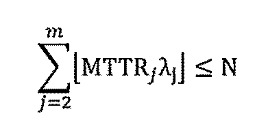
[2]代替装置(図33に示すm6)が、常用装置で最後にPMを開始する装置(図33ではm5)でPMを終了した後に、後続周期で1回以上処理を行った後にPMを行う場合、代替装置が第1周期で代替する回数は、条件(1)と(2)を合わせて、
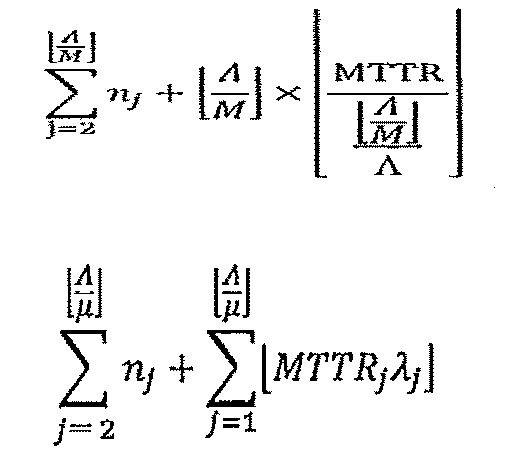
であり、第2周期以降は、このうち第2項目のみが必要となる。
条件(3)について、代替装置において、第(k-1)周期の終了時における残り代替可能回数は、下式の左辺で表される。代替可能回数は、正値でなければならないので、下式の条件となる。

この左辺で示した残り代替可能回数が、次の1周期で必要な代替回数より小さくなる周期で代替装置はPMになる。

となる最小のk’周期目に、代替装置のPMをする必要がある。
さて、ここで、図38の右側で示したように常用装置のPMを順次実施し、その期間に処理すべきロットを代替装置で処理していくと、[Λ/μ]台目の装置のPMを終了する前に、代替装置でPMが必要になる。これは、常用装置と代替装置が同時期にPMになることを意味するため、望ましくない。そこで、代替装置のPMが必要になるk’周期目では、常用装置のPMが開始する前に、代替装置のPMを終える必要がある。
第k’周期において、代替装置がPM開始前に処理可能な回数N’は、下式で表される。

この回数分を、常用装置がPMを開始する前に、意図的に処理し終えて、代替装置がPMを終了することができれば、代替装置のPMと常用装置のPMを同時期に発生せずに済む。
そこで、代替装置の残り可能処理数を常用装置の代替処理にあて、代替装置を意図的に事前にPMさせることを考える。常用装置は、第1周期ですでにそれぞれのPMが分散化するように調整がなされているため、最後にPMを終了する装置から順次、代替装置に処理を代替させる。
ここで、常用装置の台数は、[Λ/μ]であるので、通常最初にPMを開始する常用装置(図40に示す例ではm1)に対する代替回数N’1は、
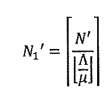
その他の常用装置(図40に示す例ではm2、m3、m4、およびm5)に対して代替する合計回数は、N’-N’1となる。
また、代替装置の処理完了回数がN’に達した時点で、代替装置のPMを行う。代替装置kのPM期間(MTTR)で処理可能なロット数は、

である。
ここで、ある周期において、常用装置の中でPMを最初に終了する装置(図40に示す例ではm1)が、PMを最後に終了する常用装置(図40に示す例ではm5)のPM終了時刻までに処理するロット数は、下式で表される。

ここで、次の周期(前の周期でPMを最後に終了する常用装置のPM終了時刻以降)に、常用装置の中で最初にPMを開始する装置が処理できるロット数は、
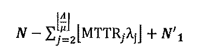
上式のロット数から代替装置による代替回数を引いた回数が、代替装置がPM終了時までの処理回数以上であれば、代替装置のPMが常用装置のPMと重ならずに済むので、下式が条件(3)の[2]の条件となる。

なお、条件(3)の[1]は、条件(3)の[2]でN’=N’1=0となる場合の特殊例で、常用装置による処理の代替を必要としない場合である。
以上、条件(1)、(2)、および(3)([1]または[2])を満たす時、JAMP法では、トラフィック強度が1を超えないようPMを分散化することができる。まず、これらの条件が満たされるか否かを調べる。満たされれば、所定の代替回数を代替装置に事前に処理させておくことでPMの時期を分散化することができる。
なお、代替装置が複数の場合には、条件(1)、(2)および(3)はそれぞれ下式のようになる。
条件(1)は、
条件(1)は、
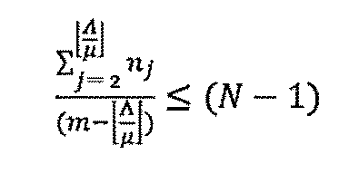
条件(2)は、
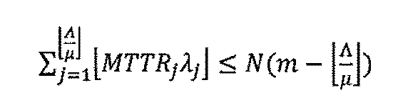
条件(1)および(2)は、
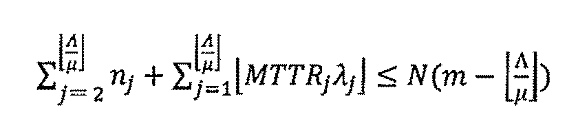
条件(3)の[1](1)、条件(3)の[2](2)については、各代替装置が負荷を担当する部分について条件が成り立つことが必要となる。
条件(3)の[1]は、
条件(3)の[1]は、

条件(3)の[2]は、

次に、条件を満たすことができず、完全にPMを分散化できない場合に、代替装置に予め負荷を代替させておくことでPMによる負の影響を軽減する方法を説明する。
本実施形態では、負荷分散方法2(条件(1)および(2)を満たさない場合)の基本的な考え方は、以下2点に集約される。
1周期目で、JAMP法による負荷分散を可能な限り適用し、PMの重複時間を低減かつ分散化する。
2周期目以降で、条件の範囲内で代替処理を行い、完全分散化をはかる。
[指針1:重複する台数・時間長の低減]
図41は、1周期で完全分散化できない場合の装置運用指針1について説明するための図である。
JAMP法のコンセプトに基づき、代替装置を用いて負荷を分散させ、可能な限り同時期にPMになる台数および時間長を抑える。
ただし、
本実施形態では、負荷分散方法2(条件(1)および(2)を満たさない場合)の基本的な考え方は、以下2点に集約される。
1周期目で、JAMP法による負荷分散を可能な限り適用し、PMの重複時間を低減かつ分散化する。
2周期目以降で、条件の範囲内で代替処理を行い、完全分散化をはかる。
[指針1:重複する台数・時間長の低減]
図41は、1周期で完全分散化できない場合の装置運用指針1について説明するための図である。
JAMP法のコンセプトに基づき、代替装置を用いて負荷を分散させ、可能な限り同時期にPMになる台数および時間長を抑える。
ただし、
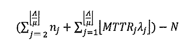
ロットについて同一周期(例えば第1周期)では代替できない。
[指針2:重複時間の分散化]
図41は、1周期で完全分散化できない場合の装置運用指針2について説明するための図である。
PM時期の重複期間が、出来るだけ連続しないよう、重なる時間長を分散化する。
図41は、1周期で完全分散化できない場合の装置運用指針2について説明するための図である。
PM時期の重複期間が、出来るだけ連続しないよう、重なる時間長を分散化する。
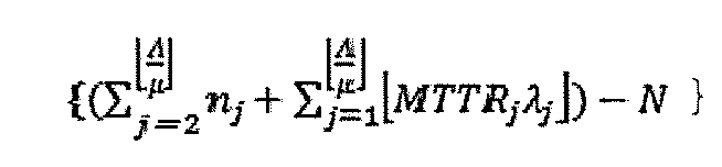
ロットを各装置に分散化する。
[指針3:PMの分散化]
2周期目以降で、完全分散化のために代替処理を施し、各装置のPM時期をずらす。
ここで、指針2における、重複時間の分散化(1周期目)について、図41を参照して説明する。
第1周期において完全には代替しきれない
第1周期において完全には代替しきれない
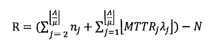
回の処理がある。
これを、1台目以外の残りの装置([Λ/μ]-1)台と代替装置(m-[Λ/μ])台でのPM時期の重なりとして分散し、工程性能が低下した状態が連続すること防ぐ。
常用装置において、PM期間が重なる処理回数

装置jの代替回数(最大)を、nj’=nj’-r(j=2、・・・[Λ/μ])とする。全てr回分ずれることになるので、実際に待ちロットを発生させるのはm1とm2の重なり部分になる。
また、残りの重なり期間の処理回数

の重なり分を以下のように配分する。なお、より細かな設定条件もあるが、ここでは省略する。
(1)e≦(m-[Λ/μ])ならば、代替装置に残り不足回数によるPM重なり期間を分配する。
(2)e>(m-[Λ/μ])ならば、常用装置に残り不足回数によるPM重なり期間を分配する。r’=r+1とし、nj’’=nj’-r’とする。
図42は、指針3の完全分散化(2周期目以降)について説明するための図である。
第一周期において完全には代替しきれなかったR回分を含めて、PM時期の重複時間をなくしていく。
装置jの代替回数(最大)は、nj’’=nj’-rまたはnj’-r’となっている。これは、各装置で、完全なPM分散化に必要な回数よりも最低r(またはr’)回の処理時間分ずつ前にずれていることになる。
ここで、第2周期目以降で、そのずれを後ろにずらし、完全分散化を図る。
ただし、JAMP法の条件を満たす範囲内で代替していく(必ず2周期目で完全分散化できるわけではない。必要な周期を使って分散化を図る。)。
第一周期において完全には代替しきれなかったR回分を含めて、PM時期の重複時間をなくしていく。
装置jの代替回数(最大)は、nj’’=nj’-rまたはnj’-r’となっている。これは、各装置で、完全なPM分散化に必要な回数よりも最低r(またはr’)回の処理時間分ずつ前にずれていることになる。
ここで、第2周期目以降で、そのずれを後ろにずらし、完全分散化を図る。
ただし、JAMP法の条件を満たす範囲内で代替していく(必ず2周期目で完全分散化できるわけではない。必要な周期を使って分散化を図る。)。
次に、JAMP法の効果をシミュレーション実験によって確かめる。
[目的と方法]
今回のシミュレーション実験の目的は、複数の装置が存在する工程において、単純に並列処理させた場合(以下、単純並列ルールと呼ぶ)と、定量メンテナンスを考慮して事前に各装置に負荷分散を行うJAMPルールの性能を比較することで、JAMPルールの効果を確かめることにある。
実験方法としては、図33に示した、ロット・シングルタスク型装置6台、一品種を想定したシミュレーション実験を行う。ここで、ロット・シングルタスク型装置とは、1ロットずつ処理を行う装置をさす。ロットは定期投入によってトラフィック強度に応じた一定間隔で到着するものとする。6台の装置の単純並列ルールによる運用については、トラフィック強度が0.8の場合、図33に示した通り通常は5台を使用し、いずれかの装置がPMなどで使用ができないときには代替装置として残りの1台を使用する。
[目的と方法]
今回のシミュレーション実験の目的は、複数の装置が存在する工程において、単純に並列処理させた場合(以下、単純並列ルールと呼ぶ)と、定量メンテナンスを考慮して事前に各装置に負荷分散を行うJAMPルールの性能を比較することで、JAMPルールの効果を確かめることにある。
実験方法としては、図33に示した、ロット・シングルタスク型装置6台、一品種を想定したシミュレーション実験を行う。ここで、ロット・シングルタスク型装置とは、1ロットずつ処理を行う装置をさす。ロットは定期投入によってトラフィック強度に応じた一定間隔で到着するものとする。6台の装置の単純並列ルールによる運用については、トラフィック強度が0.8の場合、図33に示した通り通常は5台を使用し、いずれかの装置がPMなどで使用ができないときには代替装置として残りの1台を使用する。
図43は、モデルの設定値を示す図である。
図43に、処理時間、工程のトラフィック強度、定量メンテナンスの開始の指針となるlot数(PM指針lot数)、予防保全の所要時間(MTTR)を示す。
MTTRの設定には、JAMPルールの条件(1)および(2)が満たせる場合が2つ(S1、S2)と、条件(1)、(2)を合わせた条件が満たせなくなる場合(S3)の計3つのシナリオを使用する。シナリオS1とS2の違いは、S1では代替装置のPMがちょうど常用装置のPMの終了時に発生する場合で、条件(3)の[1]に該当する。
S2は代替装置のPMが何も調整を加えないと他の装置のPMの時期と重なってしまうため条件(3)の[2]を適用して待ち時間の発生を抑える必要がある場合となっている。S3は、必ず2台以上のPMが同時に発生する必要がある場合となっている。S3は、実際の工場のPM条件設定(100lot処理を終える毎にPMのため24時間停止する)に相当する。
以上のようなモデルを用いて、単純並列とJAMPの二つのルールについて実験を行い、結果について比較する。
図43に、処理時間、工程のトラフィック強度、定量メンテナンスの開始の指針となるlot数(PM指針lot数)、予防保全の所要時間(MTTR)を示す。
MTTRの設定には、JAMPルールの条件(1)および(2)が満たせる場合が2つ(S1、S2)と、条件(1)、(2)を合わせた条件が満たせなくなる場合(S3)の計3つのシナリオを使用する。シナリオS1とS2の違いは、S1では代替装置のPMがちょうど常用装置のPMの終了時に発生する場合で、条件(3)の[1]に該当する。
S2は代替装置のPMが何も調整を加えないと他の装置のPMの時期と重なってしまうため条件(3)の[2]を適用して待ち時間の発生を抑える必要がある場合となっている。S3は、必ず2台以上のPMが同時に発生する必要がある場合となっている。S3は、実際の工場のPM条件設定(100lot処理を終える毎にPMのため24時間停止する)に相当する。
以上のようなモデルを用いて、単純並列とJAMPの二つのルールについて実験を行い、結果について比較する。
今回シミュレーション実験における2つのルールの設定について、以下に説明する。図44は、JAMPにおける代替回数設定について説明するための図である。
単純並列ルールは、図37のように最初にm1、m2、…、m5の5台で、到着間隔に起因して1/Λずつズレが起きる以外は、100lot目までm1~m5台目の5台で単純に並列処理を行い、1~5台目のいずれかがPMを行う期間はm6または他の装置の中で最も早く処理を開始できる装置が処理を代替する。
単純並列ルールは、図37のように最初にm1、m2、…、m5の5台で、到着間隔に起因して1/Λずつズレが起きる以外は、100lot目までm1~m5台目の5台で単純に並列処理を行い、1~5台目のいずれかがPMを行う期間はm6または他の装置の中で最も早く処理を開始できる装置が処理を代替する。
JAMPルールは、図38に示すように、定量メンテナンスを考慮しながら事前にジョブの代替処理を行っておきPMを分散するルールで、単純並列ルールと同様に1/Λずつズレが起きる他に、PMが2台以上重なることを防ぐために、図38のようにm1がPMを開始する前に代替装置m6にm2~m5の処理数量を代替させることで、m1~m5の5台の装置のPMを同時期に起こさずに、PMで休止する装置を常に1台以下に抑えるように負荷分散する。図39にJAMP法の条件(3)の[2]の説明図を示す。図43に、本実験の設定条件下でJAMPルールを用いる場合の代替回数を示す。
ここで、1周期とは、m1が最初のロットの処理を開始してから、m5がMTTRを終えるまでの期間を指す(図40参照)。シナリオS3は、PM指針の100を超えているので、1周期で完全分散化が出来ない場合に該当する。
[結果・考察]
図44は、JAMP法における代替え回数の設定について説明するための図である。図51は、単純並列ルールとJAMPルールの比較について説明するための図である。
図43、図44で示した設定で、2つのルールについて3つのシナリオでシミュレーション実験を行った。代替装置がPMを実施する周期の終了までの結果を図45に示す。ここでは、性能評価指標として、PMによる待ちが発生したロット数、サイクルタイム、Q-time制約を超過したロット数の3点を挙げた。
[結果・考察]
図44は、JAMP法における代替え回数の設定について説明するための図である。図51は、単純並列ルールとJAMPルールの比較について説明するための図である。
図43、図44で示した設定で、2つのルールについて3つのシナリオでシミュレーション実験を行った。代替装置がPMを実施する周期の終了までの結果を図45に示す。ここでは、性能評価指標として、PMによる待ちが発生したロット数、サイクルタイム、Q-time制約を超過したロット数の3点を挙げた。
図45に示すように、代替装置で負荷分散、PMを終える周期までの結果として、S1では9周期までの結果を、S2、S3についてはそれぞれ3、4周期目までの結果を示した。
生産期間(観測周期)が長くなると、上表の値に比例して、単純並列とJAMPとの差が広がっていく。
以上の実験結果からJAMPルールでは、シナリオS1、S2ではPMによるロットの待ちが発生せず、Q-time制約を超過するロットがないことがわかる。特に待ち時間の総計から、単純並列ルールでは、長時間の待ちが発生している一方でJAMPルールでは待ちを発生せずに済んだことが分かる。
また、待ちが発生したロット数の総計から、単純並列ルールでは、毎周期待ちlotが発生しており、時間を追うごとにこの差は広がっていく。これらの性能評価の結果から、JAMPルールではPMを分散することによって、トラフィック強度が1より大きくなることを抑え、PMに起因するロットの待ち時間の発生を抑え、Q-time制約を超過するロットの発生も抑えることができること、を確かめることができた。
生産期間(観測周期)が長くなると、上表の値に比例して、単純並列とJAMPとの差が広がっていく。
以上の実験結果からJAMPルールでは、シナリオS1、S2ではPMによるロットの待ちが発生せず、Q-time制約を超過するロットがないことがわかる。特に待ち時間の総計から、単純並列ルールでは、長時間の待ちが発生している一方でJAMPルールでは待ちを発生せずに済んだことが分かる。
また、待ちが発生したロット数の総計から、単純並列ルールでは、毎周期待ちlotが発生しており、時間を追うごとにこの差は広がっていく。これらの性能評価の結果から、JAMPルールではPMを分散することによって、トラフィック強度が1より大きくなることを抑え、PMに起因するロットの待ち時間の発生を抑え、Q-time制約を超過するロットの発生も抑えることができること、を確かめることができた。
シナリオS1とS2のようにJAMPルールで条件(1)および条件(2)を合わせた条件を満たす場合には、第1周期において、条件(1)に対する代替処理を代替装置で行い予めPMの開始時点を調整するため、2周目以降では、条件(1)に関する処理の代替は必要なくなる。2周目以降では、代替装置で条件(2)のための処理の代替と、条件(3)に示した通り、代替装置のPM時期を常用装置のPM時期と重ならないために装置間で処理の代替を行う操作を行う。これらの操作によって、JAMPルールにおける待ち時間は発生しないことが確かめられた。
JAMPルールに関して、シナリオS1の場合、条件(3)の[1]に該当する。即ち、代替装置m6が100lot目の処理を完了しPMに入るまでの期間は、代替装置m6における代替処理回数が1周期目に30回、2週目以降1周期ごとに10回代替するので、代替装置m6における処理回数が100lot目に達する時点は、8周期目で常用装置5台すべてのPMが終わる時点30+10+10+10+10+10+10+10=100で、代替装置m6がPMに入るので常用装置に影響はなかった。代替装置m6がPMを開始する時点で、装置m1はすでに4MTTR期間分の処理2x4=8ロット分になっているので、次のPMが開始するまでの残り処理可能回数は100-8=92回である。
一方、2周期以降の代替回数10回と代替装置がPM期間に装置1台当たりの処理回数2回の合計12回は、次にPMを開始する常用装置m1の残り処理回数92回に対して小さいため、十分余裕をもってPMを終えることができる。2周目以降では、常用装置m2~m5までの装置で事前に処理を代替しておく必要はないので、これで問題なくすべての装置のPMが分散化され、同時にPMを行う装置は1台以下となった。
一方、シナリオS2の場合を用いて、代替装置m6が2周期目以降の周期の途中で代替装置の100lotに達してPMに入る場合の結果を示した。この場合、何も対処をしないと、常用装置のPM中に代替装置のPMも開始することになるため、待ちロットが発生することになる。この場合に対処するため、条件(3)の[2]が必要となる。この条件(3)の[2]で、2周目以降も、意図的に代替装置のPM時期を調整するために他の装置の代替を行うことによって、複数の装置のMTTRが重ならないように調整することができる。S2の場合、1周目で装置m1~m5のPMが同時期に重ならないようにずらすための事前の処理代替回数が60回、また装置m1~m5がMTTRの期間に処理を代替するために35回の代替回数が必要となっている。代替装置は、2周目であと残りの100-95=5回代替した時点でPMを開始する必要がある。
2周目では、本来は事前に処理を代替する必要がないので、何もしなければ、m1のPM時に処理を5回代替した時点でm6の装置がPMを開始しなければならず、m6のPMの期間MTTRの間は2台の装置がPMになる。これを防ぐために、2周期目でm1がPMを始める前に代替装置m6のPMを完了しておくことが必要である。そのため、m5のPMが終了した時点(この時点までにm1は、28lot処理している)から、装置m6がm1からm5の装置の代替を1回ずつ行う(これが終わるまでに、m1は28+4=32lot処理する)。これが終了した時点でm6はPMを開始する。MTTR経過後m6は使用可能となる(この時点までにm1は、32+7=39lot処理する)。この時点では、最もPMが起こりやすい装置m1でも、まだ39lotしか処理を終えておらず、定量メンテナンスの指針ロット数100以下であるため、すべての装置のPMを分散することができる。実験結果から、条件(3)の[2]に該当する場合にも、PMを分散化でき、PMによるロットの待ち時間の発生を完全に抑えることができることが確かめられた。
最後に、シナリオS3では、条件(1)と(2)を合わせた条件が成り立たない。つまり、1周期目で複数の装置がPMに入らざるを得ない状況が発生する。しかし、この場合でも代替装置を用いてできる限りPMの分散化を図っておくことによって、PMによるロットの待ち時間を抑え、Q-time制約割れをゼロに抑えられることができることが確かめられた。シナリオS3は、実際の工場における定量メンテナンスの設定であり、効果が期待できる。
JAMP法は、PMによる工程の生産能力の低下を最低限に抑えて変動を抑制し、生産の平準化を指向した方法である。そのため、後続工程では、ロットの到着が平準化される(図46:終了時刻)
図46は、ロットの到着と退去の時刻(JAMP法と単純並列ルールの比較)を示す図である。他方の単純並列の問題として、生産の能力の増減(変動)が大きく(下図)、仕掛数の急激な増加と、後続工程への流量の変動(上図)をもたらす。
図47は、装置台数の稼働状況の変動(単純並列 MTTR=1380[分]の場合)を示す図である。以上のことから定量メンテナンスを考慮したジョブの割り付け方法JAMPの効果が示された。
図46は、ロットの到着と退去の時刻(JAMP法と単純並列ルールの比較)を示す図である。他方の単純並列の問題として、生産の能力の増減(変動)が大きく(下図)、仕掛数の急激な増加と、後続工程への流量の変動(上図)をもたらす。
図47は、装置台数の稼働状況の変動(単純並列 MTTR=1380[分]の場合)を示す図である。以上のことから定量メンテナンスを考慮したジョブの割り付け方法JAMPの効果が示された。
[結論]
本実施形態では、定量メンテナンスのある処理工程を取り上げ、同時期に予防保全になる装置台数を出来るだけ少なくする装置の負荷分散方法を開発し、その効果を確かめることを目的として研究を行った。
本実施形態では、新たに、負荷分散法JAMP(Job Allocation for Maintenance in Parallel)法を提案した。JAMP法の効果を確かめるために、実際の工場の工程モデルを参考にして、シミュレーション実験により単純並列ルールとの比較を行った。シミュレーションモデルは、6台の装置で処理時間が所与の1品種を処理する工程で、工程のトラフィック強度が0.8になるよう定期投入が行われる連続処理のモデルを用いた。
実験では、JAMPによって同時期にPMになる装置台数を1台以下に抑え完全に分散化できる(トラフィック強度を常に1未満に抑えられる)場合と、完全にはPMの分散化ができない(常にはトラフィック強度を1未満に抑えられない)場合の2つの場合を設定して、それぞれにおけるJAMPの効果を確かめた。
本実施形態では、定量メンテナンスのある処理工程を取り上げ、同時期に予防保全になる装置台数を出来るだけ少なくする装置の負荷分散方法を開発し、その効果を確かめることを目的として研究を行った。
本実施形態では、新たに、負荷分散法JAMP(Job Allocation for Maintenance in Parallel)法を提案した。JAMP法の効果を確かめるために、実際の工場の工程モデルを参考にして、シミュレーション実験により単純並列ルールとの比較を行った。シミュレーションモデルは、6台の装置で処理時間が所与の1品種を処理する工程で、工程のトラフィック強度が0.8になるよう定期投入が行われる連続処理のモデルを用いた。
実験では、JAMPによって同時期にPMになる装置台数を1台以下に抑え完全に分散化できる(トラフィック強度を常に1未満に抑えられる)場合と、完全にはPMの分散化ができない(常にはトラフィック強度を1未満に抑えられない)場合の2つの場合を設定して、それぞれにおけるJAMPの効果を確かめた。
その結果、完全にPMを分散化できる場合にはPMによる待ち時間をゼロに抑えることができ、また、完全にPMを分散化できない場合でも、JAMPが同時期にPMになる装置の台数を可能な限り少なくするよう働くため、結果として単純並列ルールに比べて優れていることが確かめられた。
ここで、特にMTTRが大きい場合には、PMによるロットの待ち時間が長くなり、Q-time制約を割ってリワークが発生する事態が生じやすくなる。リワークの発生は生産上のロスでしかなく、副次的に正規ロットの生産物流を阻害するため望ましくない。このQ-time制約割れを防ぐためにも、同時期にPMになる台数を少なくすることで工程のトラフィック強度を常にできる限り低く抑え、余計な待ち時間を発生させないことによって、Q-time割れロットの数を抑えることができることが確認できた。
本提案法は、定量メンテナンスだけでなく、定期メンテナンスの分散化にも活用できる。
ここで、特にMTTRが大きい場合には、PMによるロットの待ち時間が長くなり、Q-time制約を割ってリワークが発生する事態が生じやすくなる。リワークの発生は生産上のロスでしかなく、副次的に正規ロットの生産物流を阻害するため望ましくない。このQ-time制約割れを防ぐためにも、同時期にPMになる台数を少なくすることで工程のトラフィック強度を常にできる限り低く抑え、余計な待ち時間を発生させないことによって、Q-time割れロットの数を抑えることができることが確認できた。
本提案法は、定量メンテナンスだけでなく、定期メンテナンスの分散化にも活用できる。
なお、実用時には、多品種生産における段取り時間やバッチ工程におけるバッチ組時間を考慮する必要がある。
その場合の条件を以下に示す。
λjを装置j一台当たりの到着率[lot/分]λj=Λ/[Λ/μ]、Λを装置群全体の到着率[lot/分]、Mを工程サービス能力=m/Tp[lot/分]、(m:装置台数、Tp:平均処理時間)、Nを定量メンテナンスの基準値[lot]、MTTRを予防保全(PM)の所要時間[分]、Ts1、Ts2を段取り時間等の合計とするとき、多品種生産における段取りを考慮した場合の条件は、以下のように表せる。
条件(1)は、
その場合の条件を以下に示す。
λjを装置j一台当たりの到着率[lot/分]λj=Λ/[Λ/μ]、Λを装置群全体の到着率[lot/分]、Mを工程サービス能力=m/Tp[lot/分]、(m:装置台数、Tp:平均処理時間)、Nを定量メンテナンスの基準値[lot]、MTTRを予防保全(PM)の所要時間[分]、Ts1、Ts2を段取り時間等の合計とするとき、多品種生産における段取りを考慮した場合の条件は、以下のように表せる。
条件(1)は、
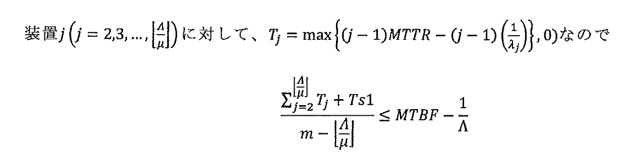
条件(2)は、

条件(1)および(2)は、

となる。
また、バッチ工程におけるバッチ組時間を考慮した条件は、以下の通りとなる。
バッチ装置においては、ロードルールによって処理開始間隔(ロード間隔)と処理単位(ロードサイズ)が異なる。1台あたりの実行サービス率は、以下の式で表せる。
1台当たりの実行サービス率=(ロードサイズ)/(ロード間隔)
装置からみた場合のロード間隔は、ロードサイズをLaとしたとき、以下のように算出できる。
1ロットが到着する時間間隔が1/Λなので、サイズLaのバッチを1つ組むまでの時間間隔は、La/Λとなる。装置のロード間隔TLは、
La/Λ>T/pm(すなわちρ<1)のときTL=Tp+(La/Λ-Tp/m)
La/Λ≦Tp/m(すなわちρ≧1)のときTL=Tp
バッチ装置においては、ロードルールによって処理開始間隔(ロード間隔)と処理単位(ロードサイズ)が異なる。1台あたりの実行サービス率は、以下の式で表せる。
1台当たりの実行サービス率=(ロードサイズ)/(ロード間隔)
装置からみた場合のロード間隔は、ロードサイズをLaとしたとき、以下のように算出できる。
1ロットが到着する時間間隔が1/Λなので、サイズLaのバッチを1つ組むまでの時間間隔は、La/Λとなる。装置のロード間隔TLは、
La/Λ>T/pm(すなわちρ<1)のときTL=Tp+(La/Λ-Tp/m)
La/Λ≦Tp/m(すなわちρ≧1)のときTL=Tp
ここで、Mを装置台数、Tpを平均処理時間、Laを平均ロードサイズ[lot]、Λを装置群全体の到着率[lot/分]、λj=Λ/[Λ/μ]である。
このTLをTpの代わりに使用して工程能力Mを計算することで、バッチ組時間を考慮することが可能となる。
なお、Laはロードルールとトラフィック強度に依存する。最大バッチサイズを満たさなくても処理を開始できるロードルールとすると、装置が空くとすぐに装置での処理が開始する(常に装置が稼働する)ように作用する。
1台の装置が空く平均時間間隔は、Tp/mで、その期間に到着するWIP数は、Tpm×Λ
計画上のサービス率μ=LTp
このTLをTpの代わりに使用して工程能力Mを計算することで、バッチ組時間を考慮することが可能となる。
なお、Laはロードルールとトラフィック強度に依存する。最大バッチサイズを満たさなくても処理を開始できるロードルールとすると、装置が空くとすぐに装置での処理が開始する(常に装置が稼働する)ように作用する。
1台の装置が空く平均時間間隔は、Tp/mで、その期間に到着するWIP数は、Tpm×Λ
計画上のサービス率μ=LTp
このLaを用いる。
なお、各変数の定義は、次の通りである。
ρ:工程利用率、L:最大バッチサイズ[lot]、La:平均ロードサイズ[lot]、Λ:装置群全体の到着率[lot/分]、λj=Λ/[Λ/μ]、ρ=Λ/mμ
第2実施形態では、JAMP法により第2問題点を解決している。
Q-time制約割れの主要な原因のである装置の予防保全時期を分散化するための装置への負荷配分方法を、JAMP(Job Allocation for Maintenance in Parallel)法と名付けた。JAMP法で、同時期に停止する装置台数を最小限に抑え、高い生産能力の維持と生産の平準化を図り、製品ロットの無駄な待ちやQ-time制約割れを抜本的に防ぐ。第2実施形態は、JAMP法のプログラムとそれを用いた性能評価結果(実際の工場のデータを用いた確定的シミュレーションによる)である。性能評価結果から、JAMP法が並列装置を順々に均等に使用する単純並列ルールに比べて、2.5ヵ月当たり188ロットのリワークを削減し、2千万円以上のリワーク費用の削減効果が見込まれ、かつ、待ちロット数を172分の1、ロットの待ち時間総計を13805分の1にまで大幅に低減できるため納期遵守にも効果がある。CKB法とJAMP法とを組み合わせて用いることで、単一Q-time制約区間の最適管理が実現される。
Q-time制約割れの主要な原因のである装置の予防保全時期を分散化するための装置への負荷配分方法を、JAMP(Job Allocation for Maintenance in Parallel)法と名付けた。JAMP法で、同時期に停止する装置台数を最小限に抑え、高い生産能力の維持と生産の平準化を図り、製品ロットの無駄な待ちやQ-time制約割れを抜本的に防ぐ。第2実施形態は、JAMP法のプログラムとそれを用いた性能評価結果(実際の工場のデータを用いた確定的シミュレーションによる)である。性能評価結果から、JAMP法が並列装置を順々に均等に使用する単純並列ルールに比べて、2.5ヵ月当たり188ロットのリワークを削減し、2千万円以上のリワーク費用の削減効果が見込まれ、かつ、待ちロット数を172分の1、ロットの待ち時間総計を13805分の1にまで大幅に低減できるため納期遵守にも効果がある。CKB法とJAMP法とを組み合わせて用いることで、単一Q-time制約区間の最適管理が実現される。
<第3実施形態>
図48を参照して、本発明の第3実施形態に係る最適指標生成装置について説明する。
本発明の第3実施形態に係る最適指標生成装置31は、例えば、半導体を生産するための生産工程#1にそれぞれ設けられた処理工程(装置群)2および処理工程(装置群)3の生産スケジュールを管理する生産管理システム10を制御の対象としている。同時に、製造装置の予防保全時期を分散化する運用方法について、生産工程#1にそれぞれ設けられた装置群5の保全スケジュールを管理する生産管理システム10やエンジニアリング業務システム29を制御の対象としている。本実施形態では、生産物流制御法と生産負荷配分法(以下、CKB-JAMP法という)について説明する。
図48を参照して、本発明の第3実施形態に係る最適指標生成装置について説明する。
本発明の第3実施形態に係る最適指標生成装置31は、例えば、半導体を生産するための生産工程#1にそれぞれ設けられた処理工程(装置群)2および処理工程(装置群)3の生産スケジュールを管理する生産管理システム10を制御の対象としている。同時に、製造装置の予防保全時期を分散化する運用方法について、生産工程#1にそれぞれ設けられた装置群5の保全スケジュールを管理する生産管理システム10やエンジニアリング業務システム29を制御の対象としている。本実施形態では、生産物流制御法と生産負荷配分法(以下、CKB-JAMP法という)について説明する。
図48に示すように、最適指標生成装置31は、図1に示す最適指標生成装置11(第1実施形態)と同様に、入力部12、補助入力部13、Q-time構造分析部14を備えている。
また、最適指標生成装置31は、図30に示す最適指標生成装置21(第2実施形態)と同様に、入力部22、補助入力部(JAMP法)23、開始終了時期算出部26、装置区分算定部28を備えている。
第1および第2実施形態と比較して、第3実施形態に特徴的な構成は、図48に示すように、変動監視検出部32、入力変更検出部33、再計算必要性判断部34、感度解析部(CKB+JAMP特性)35、CKB+JAMP最適論理値計算部36、感度解析部(CKB+JAMP性能特性)37を備えていることにある。
また、最適指標生成装置31は、図30に示す最適指標生成装置21(第2実施形態)と同様に、入力部22、補助入力部(JAMP法)23、開始終了時期算出部26、装置区分算定部28を備えている。
第1および第2実施形態と比較して、第3実施形態に特徴的な構成は、図48に示すように、変動監視検出部32、入力変更検出部33、再計算必要性判断部34、感度解析部(CKB+JAMP特性)35、CKB+JAMP最適論理値計算部36、感度解析部(CKB+JAMP性能特性)37を備えていることにある。
ここで、第3実施形態に特徴的な上記構成について説明する。
変動監視検出部32は、ロットの処理開始・終了、装置の状態変化(故障等に伴う)と装置群の処理能力の変化など、イベント・状態データ更新による変動を監視・検出し、変動情報を計算必要性判定部34に出力する。
変動監視検出部32は、ロットの処理開始・終了、装置の状態変化(故障等に伴う)と装置群の処理能力の変化など、イベント・状態データ更新による変動を監視・検出し、変動情報を計算必要性判定部34に出力する。
入力変更検出部33は、CKB法関連の入力データやJAMP法関連の入力データを入力し、前回のCKB法関連の入力データやJAMP法関連の入力データから変化した部分を検出し、変化があった入力データを出力する。
再計算必要性判断部34は、記憶部34aに記憶しておいた予め計算された感度解析結果における整数の閾値を入力し、入力変更検出部33で検出された変動に対して、再計算が必要であるか否かを判断する。再計算必要性判断部34は、前回の範囲の上下限の閾値を外れる場合には、再計算が必要と判断する。
CKB+JAMP最適論理値計算部36は、Q-time制約構造分析部と入力部(JAMP法)から入力データを受け取り、Q-time制約区間内の装置群に対してJAMP法理論値計算により各装置の処理負荷(回数)とその処理時期を算出し、装置群における処理能力の時間推移を、1サイクル分算定し、その期間内で区間内の処理能力や生産負荷(または生産目標)が切り替わる毎のCKB法最適理論値計算を行う。ここで、1サイクルは、全ての常用装置が1回以上かつ全ての代替装置が1回ずつ予防保全を完了するまでの期間(または別途指定された生産期間)などとする。
更に、CKB+JAMP最適理論値計算では、装置群の処理能力の変化に応じて、予めQ-time制約区間における投入量をQ-time制約を遵守できる値として変更する機能を備え、円滑なQ-time区間の管理を実現する。
更に、CKB+JAMP最適理論値計算では、装置群の処理能力の変化に応じて、予めQ-time制約区間における投入量をQ-time制約を遵守できる値として変更する機能を備え、円滑なQ-time区間の管理を実現する。
図49を参照して、最適理論値計算部36の動作を説明する。ある工程(例えば、Q-time制約区間内のボトルネックの装置群)において、全ての装置が稼働可能な期間は、工程のトラフィック強度は平均的に1(100%)未満に保たれる。(そうなるように生産計画がなされる。)この時期には、処理工程に到着する全てのロットが、ある一定の滞在時間以下で処理を終了することができる。ここで、いずれかの装置が予防保全になる期間には、工程(装置群)の処理能力が低下する。場合によっては、この期間には、工程のトラフィック強度が1(100%)を超える。そして、この期間が長くなれば、Q-time制約はいずれ遵守できなくなる。このような状況を避けるために、JAMP法によって、予防保全の分散化をはかるのであるが、可動時間に対して予防保全時間が比較的長い場合などには、あらゆる場合に工程のトラフィック強度を1以下に抑えられるとは限らない。そのため、Q-time制約区間の生産流量を、工程の処理能力の変化に合わせて見直す機能を備える。
また、CKB法のようにQ-time制約を守りつつ、Q-time制約区間のスループットを可能な限り高めるために、制約を守れる最大限のロットをQ-time制約区間に滞在させる。このような場合には、工程の処理能力が低下する前にQ-time制約区間に投入されたロットが、Q-time制約を守れなくなる。
そのため、処理能力が低下する前に、予め適切な時期にQ-time制約区間へのロットの投入率を減らす。
他方で、予防保全が完了した後には、処理能力が向上し、装置を可能な限り稼働させて溜まった中間在庫を解消しようとする。この時も、予め当該工程へのロット投入を増加させておかなければ、装置復旧後の処理能力・時間が無駄になる。
これらを考慮の上、工程能力が異なる各期間に合わせた、それぞれの適正理論値計算を行い、かつ、その工程能力の変化に合わせて投入を調整するための移行期間も含めて理論値の改編時期を適切に算定する。
そのため、処理能力が低下する前に、予め適切な時期にQ-time制約区間へのロットの投入率を減らす。
他方で、予防保全が完了した後には、処理能力が向上し、装置を可能な限り稼働させて溜まった中間在庫を解消しようとする。この時も、予め当該工程へのロット投入を増加させておかなければ、装置復旧後の処理能力・時間が無駄になる。
これらを考慮の上、工程能力が異なる各期間に合わせた、それぞれの適正理論値計算を行い、かつ、その工程能力の変化に合わせて投入を調整するための移行期間も含めて理論値の改編時期を適切に算定する。
ここで、図49を用いて、工程能力が異なる各期間や移行期間の区分の方法を説明する。
まず、JAMP法により予防保全の時期と各期の工程能力が決定される。この算定結果に基づき、工程能力の異なる期間を大区分で3つに分ける。第1期間は定常期で、ロットの到着率をΛ、定常期の処理工程のサービス率をμ1、とすると平均的にμ1=Λの状態である。
次に、第2期間は低下期で、予防保全等により処理工程のサービス率が低下する期間である。低下期のサービス率をμ2とすると平均的にμ2<Λの状態にある(JAMP法などによりこのような状態の発生を防ぐことができなかった場合)。
次に、第3期は復旧期で、第2期の低下期にたまった中間在庫を早急に解消するために、最大限のサービス率で処理工程を運用する。復旧期のサービス率をμ3とするとき、平均的にμ3>Λの状態にある。
まず、JAMP法により予防保全の時期と各期の工程能力が決定される。この算定結果に基づき、工程能力の異なる期間を大区分で3つに分ける。第1期間は定常期で、ロットの到着率をΛ、定常期の処理工程のサービス率をμ1、とすると平均的にμ1=Λの状態である。
次に、第2期間は低下期で、予防保全等により処理工程のサービス率が低下する期間である。低下期のサービス率をμ2とすると平均的にμ2<Λの状態にある(JAMP法などによりこのような状態の発生を防ぐことができなかった場合)。
次に、第3期は復旧期で、第2期の低下期にたまった中間在庫を早急に解消するために、最大限のサービス率で処理工程を運用する。復旧期のサービス率をμ3とするとき、平均的にμ3>Λの状態にある。
ここで、Q-time制約が付された区間では、第1期(定常期)から第2期(低下期)、第2期(低下期)から第3期(復旧期)、第3期(復旧期)から第1期(定常期)、が切り替わる以前のTd、Tr、Tkの時点で、予め工程への到着率を適切に変更させる必要がある。
ここで、定常期から低下期へ切り替わる時点をT1、低下期から定常記に切り替わる時点をT2、復旧期から定常期に切り替わる時点をT3とする。定常期において、ロットの到着から処理開始までの滞在時間をTwと設定しているものとし、この区間でのQ-time制約による制限時間がTqであるとする。
ここで、定常期から低下期へ切り替わる時点をT1、低下期から定常記に切り替わる時点をT2、復旧期から定常期に切り替わる時点をT3とする。定常期において、ロットの到着から処理開始までの滞在時間をTwと設定しているものとし、この区間でのQ-time制約による制限時間がTqであるとする。
i)定常期から低下期への切り替えに関して
(A)Tw=Tqの場合には、Td=T1-Tw
(B)Tw<Tqの場合には、Td=T1+(μ2Tq-μ1Tw)/(μ1-μ2)
滞在時間をTq以下に抑えるためには、遅くともTdの時点で、到着率をμ1からμ2へ変更するよう制御する。
なお、
(C)Tw>Tqの場合には、常にQ-time制約が遵守できなくなるので、この場合はまずCKB法により(A)または(B)の条件を満たす状態になるように物流制御する必要がある。
(A)Tw=Tqの場合には、Td=T1-Tw
(B)Tw<Tqの場合には、Td=T1+(μ2Tq-μ1Tw)/(μ1-μ2)
滞在時間をTq以下に抑えるためには、遅くともTdの時点で、到着率をμ1からμ2へ変更するよう制御する。
なお、
(C)Tw>Tqの場合には、常にQ-time制約が遵守できなくなるので、この場合はまずCKB法により(A)または(B)の条件を満たす状態になるように物流制御する必要がある。
ii)低下期から復旧期の切り替えに関しては、
(A)Tw=Tqの場合には、Tr=T2-Tw
(B)Tw<Tqの場合には、Tr=T2-Tq
早くともTrの時点以降で、到着率をμ2からμ3へ変更するよう制御する。
(A)Tw=Tqの場合には、Tr=T2-Tw
(B)Tw<Tqの場合には、Tr=T2-Tq
早くともTrの時点以降で、到着率をμ2からμ3へ変更するよう制御する。
iii)復旧期から定常期への切り替えに関しては、
(A)Tw=Tqの場合には、Tk=T3-Tw
(B)Tw<Tqの場合には、Tk=T3-(μ3Tq-ΛTw)/(μ3-Λ)
早くともTkの時点以降で、到着率をμ3からΛ(=μ1)へ変更するよう制御する。
(A)Tw=Tqの場合には、Tk=T3-Tw
(B)Tw<Tqの場合には、Tk=T3-(μ3Tq-ΛTw)/(μ3-Λ)
早くともTkの時点以降で、到着率をμ3からΛ(=μ1)へ変更するよう制御する。
感度解析部(CKB+JAMP特性)35は、CKB法、JAMP法の感度分析部に基づいているが、本感度分析(CKB+JAMP性能特性)の特徴は、前記CKB+JAMP最適論理値計算部36での特徴と同様に、工程能力が異なる各期間やその移行期間別に、全ての対象期間について、感度解析を行うことを特徴とする。内部記憶部35aの情報は、最適指標生成31の実行必要性の判定にも用いられる。この必要性の判定は、管理対象の生産工程#1および#2における各種の変動(装置群の処理能力の変化や、目標生産率の変更、トラフィックの変動、Q-time制約の変更・追加など)に対応して判断される。必要性が確認された場合、最適指標生成31に計算指示が出される。
感度解析部(CKB+JAMP性能特性)37は、CKB法、JAMP法の感度分析部に基づいているが、本感度分析(CKB+JAMP性能特性)の特徴は、前記感度解析部(CKB+JAMP特性)35での特徴と同様に、工程能力が異なる各期間やその移行期間別に、全ての対象期間について、感度解析における性能評価を行うことを特徴とする。
感度解析部(CKB+JAMP性能特性)37は、CKB法、JAMP法の感度分析部に基づいているが、本感度分析(CKB+JAMP性能特性)の特徴は、前記感度解析部(CKB+JAMP特性)35での特徴と同様に、工程能力が異なる各期間やその移行期間別に、全ての対象期間について、感度解析における性能評価を行うことを特徴とする。
図48を参照して、本発明の第3実施形態に係る最適指標生成装置31の動作について説明する。
生産実行システムに含まれる複数の装置に関する情報を生産管理システム10を介して入力部12、により入力し、入力された情報から複数の装置による加工工程間の滞在時間の上限値や下限値を示すQ-time構造をQ-time構造分析部14により分析し、各Q-time制約に対して、製品の到着に関連するバッチ組待ち時間とQ-time制約の上限値との大小関係が切り替わる到着率の境界値を算定し、適切なロードルールを判定し、生産管理システム10を介して入力部22から入力された生産実行システムに含まれる複数の常用装置と代替装置に関する情報から複数の装置を装置区分算定部28により常用装置と代替装置とに区分し、複数の装置の稼働回数と稼働時期を算出するとともに、常用装置と代替装置とに関する予防保全開始時間を算出し、算出された予防保全時期と入力された情報およびQ-time構造に基づいて、品種別の最適なカンバン枚数およびバッファサイズを計算して指標情報として指標算出部17により出力し、常用装置と代替装置とに関する稼働回数と稼働時期と予防保全開始時間を開始終了時期算出部26により算出し、指標算出部17により算出された最適な指標情報を生産管理システム10に供給するとともに、開始終了時期算出部26により算出された最適な開始終了時期情報を生産管理システム10に供給する。
生産実行システムに含まれる複数の装置に関する情報を生産管理システム10を介して入力部12、により入力し、入力された情報から複数の装置による加工工程間の滞在時間の上限値や下限値を示すQ-time構造をQ-time構造分析部14により分析し、各Q-time制約に対して、製品の到着に関連するバッチ組待ち時間とQ-time制約の上限値との大小関係が切り替わる到着率の境界値を算定し、適切なロードルールを判定し、生産管理システム10を介して入力部22から入力された生産実行システムに含まれる複数の常用装置と代替装置に関する情報から複数の装置を装置区分算定部28により常用装置と代替装置とに区分し、複数の装置の稼働回数と稼働時期を算出するとともに、常用装置と代替装置とに関する予防保全開始時間を算出し、算出された予防保全時期と入力された情報およびQ-time構造に基づいて、品種別の最適なカンバン枚数およびバッファサイズを計算して指標情報として指標算出部17により出力し、常用装置と代替装置とに関する稼働回数と稼働時期と予防保全開始時間を開始終了時期算出部26により算出し、指標算出部17により算出された最適な指標情報を生産管理システム10に供給するとともに、開始終了時期算出部26により算出された最適な開始終了時期情報を生産管理システム10に供給する。
これにより、従来法では達成されていなかったQ-time制約割れが起こりやすい状況に対しても、Q-time制約を確実に遵守し、良品スループット向上とコスト低減および環境負荷低減を達成することが可能な最適オペレーション管理条件を提供することができる。
また、Q-time制約割れの主要な原因である、多品種生産の扱い、装置の予防保全、複数のQ-time制約の相互干渉に対しても、解析方法と適正な管理手法を与えることで、Q-time制約遵守しつつ良品スループットの向上とコスト低減・環境負荷低減を同時に達成することができる。
また、Q-time制約割れの主要な原因である、多品種生産の扱い、装置の予防保全、複数のQ-time制約の相互干渉に対しても、解析方法と適正な管理手法を与えることで、Q-time制約遵守しつつ良品スループットの向上とコスト低減・環境負荷低減を同時に達成することができる。
<第4実施形態>
図50を参照して、本発明の第4実施形態に係る最適指標生成装置について説明する。
本発明の第4実施形態に係る最適指標生成装置41は、例えば、半導体を生産するための生産工程#1にそれぞれ設けられた処理工程(装置群)2および処理工程(装置群)3の生産スケジュールを管理する生産管理システム10を制御の対象としている。同時に、製造装置の予防保全時期を分散化する運用方法について、生産工程#1にそれぞれ設けられた装置5の保全スケジュールを管理する生産管理システム10を制御の対象としている。本実施形態では、連動型生産物流制御法(以下、手続き型CKB法という)について説明する。
図50を参照して、本発明の第4実施形態に係る最適指標生成装置について説明する。
本発明の第4実施形態に係る最適指標生成装置41は、例えば、半導体を生産するための生産工程#1にそれぞれ設けられた処理工程(装置群)2および処理工程(装置群)3の生産スケジュールを管理する生産管理システム10を制御の対象としている。同時に、製造装置の予防保全時期を分散化する運用方法について、生産工程#1にそれぞれ設けられた装置5の保全スケジュールを管理する生産管理システム10を制御の対象としている。本実施形態では、連動型生産物流制御法(以下、手続き型CKB法という)について説明する。
図50に示すように、最適指標生成装置41は、図1に示す最適指標生成装置11(第1実施形態)と同様に、入力部12、補助入力部13、指標算出部17を備えている。
また、最適指標生成装置41は、図30に示す最適指標生成装置21(第2実施形態)と同様に、入力部22、補助入力部23、開始終了時期算出部26を備えている。
さらに、最適指標生成装置41は、図48に示す最適指標生成装置31(第3実施形態)と同様に、変動監視検出部32、入力変更検出部33、再計算必要性判断部34、感度解析部(CKB+JAMP特性)35、CKB+JAMP最適論理値計算部36、感度解析部(CKB+JAMP性能特性)37を備えている。
第1、第2および第3実施形態と比較して、第4実施形態に特徴的な構成は、図50に示すように、生産フローボトルネック・流量解析部42、Q-time構造分析部43、装置区分算定部44、補助入力部(手続き型CKB法)45、駆動制御部46、余裕時間配分解析部47、手続き実行制御部(CKB+PS法)48を備えていることにある。なお、駆動制御部46は、変動監視検出部32、入力変更検出部33、再計算必要性判断部34、感度解析部(CKB+JAMP特性)35から構成されている。
また、最適指標生成装置41は、図30に示す最適指標生成装置21(第2実施形態)と同様に、入力部22、補助入力部23、開始終了時期算出部26を備えている。
さらに、最適指標生成装置41は、図48に示す最適指標生成装置31(第3実施形態)と同様に、変動監視検出部32、入力変更検出部33、再計算必要性判断部34、感度解析部(CKB+JAMP特性)35、CKB+JAMP最適論理値計算部36、感度解析部(CKB+JAMP性能特性)37を備えている。
第1、第2および第3実施形態と比較して、第4実施形態に特徴的な構成は、図50に示すように、生産フローボトルネック・流量解析部42、Q-time構造分析部43、装置区分算定部44、補助入力部(手続き型CKB法)45、駆動制御部46、余裕時間配分解析部47、手続き実行制御部(CKB+PS法)48を備えていることにある。なお、駆動制御部46は、変動監視検出部32、入力変更検出部33、再計算必要性判断部34、感度解析部(CKB+JAMP特性)35から構成されている。
ここで、第4実施形態に特徴的な上記構成について説明する。
生産フローボトルネック・流量解析部42は、生産実行システムに含まれる製造フロー全体における生産流量や工程能力の変動に対応してQ-time制約を同時に管理するために、工程の接続行列(生産フロー)、工程の処理容量行列、Q-time制約区間の許容流量を入力し、TOC理論または最大流問題・最小カット定理などを用いて、生産フロー統合解析、ボトルネック箇所検出、最大流量計算を行う。生産フローボトルネック・流量解析部42は、ボトルネック箇所(最小カットに該当する工程群)、各処理工程における流量(処理負荷)を出力する。
生産フローボトルネック・流量解析部42は、生産実行システムに含まれる製造フロー全体における生産流量や工程能力の変動に対応してQ-time制約を同時に管理するために、工程の接続行列(生産フロー)、工程の処理容量行列、Q-time制約区間の許容流量を入力し、TOC理論または最大流問題・最小カット定理などを用いて、生産フロー統合解析、ボトルネック箇所検出、最大流量計算を行う。生産フローボトルネック・流量解析部42は、ボトルネック箇所(最小カットに該当する工程群)、各処理工程における流量(処理負荷)を出力する。
Q-time構造分析部43は、CKB法の入力データおよびJAMP法の入力データ、工程接続のデータ(生産フロー)、工程の処理能力データ、Q-time制約データ、工程における生産品種別の処理負荷を入力する。そして、Q-time構造分析部43は、どのQ-time制約区間の構造に該当するかを検出し(直列型4種、並列型5種)てQ-time制約の構造を分析する。同時に、Q-time構造分析部43は、特別な処理(3工程以上に跨る排他、中間工程重複の場合)を必要とするQ-time制約区間に該当するか否かチェックする。
Q-time構造分析部43は、各Q-time制約区間の範囲と構造(Q-time制約区間の開始・終了工程、構造No、など)を出力し、特別構造フラグ(ON=1)を立てる。
Q-time構造分析部43は、各Q-time制約区間の範囲と構造(Q-time制約区間の開始・終了工程、構造No、など)を出力し、特別構造フラグ(ON=1)を立てる。
装置区分算定部44は、第2実施形態において用いた装置区分算定部28と同様である。
補助入力部45は、CKB+JAMP最適理論値計算36、余裕時間配分解析部47、駆動制御部46で使用するデータを生産管理システムやエンジニアリング業務システムから入力する。
駆動制御部46は、生産工程の動的変化に合わせて管理をするために、変動監視検出部32で生産管理システムから最新の生産計画・実績情報を入力して、入力変更検出部33で各Q-time制約区間に対する変化を検出して、再計算必要性判定部34でCKB法の再計算が必要か否かを判定する。必要であると判定された場合には、手続き実行制御部48などに再計算指示を入力し、図53に示す手続き型CKB法のS22からS25までの処理を再実行し、CKB法の最適理論値を再計算する。
駆動制御部46は、生産工程の動的変化に合わせて管理をするために、変動監視検出部32で生産管理システムから最新の生産計画・実績情報を入力して、入力変更検出部33で各Q-time制約区間に対する変化を検出して、再計算必要性判定部34でCKB法の再計算が必要か否かを判定する。必要であると判定された場合には、手続き実行制御部48などに再計算指示を入力し、図53に示す手続き型CKB法のS22からS25までの処理を再実行し、CKB法の最適理論値を再計算する。
余裕時間配分解析部47は、補助入力部45からの入力に応じて、Q-time制約区間における余裕時間配分の箇所(工程間)と時間長を、各工程の装置台数やサービス能力および生産物流の状態などから算定する。手続き型CKB法(標準)に追加の手続きを要する構造については、図55のように条件分岐付き手続きで管理する。追加の手続きを要する構造とは、図52の直列型(C)重複に該当する複数のQ-time制約、または、単一Q-time制約区間が3工程以上にまたがる場合(並列構造においては、直列型に変換した際に、上述の構造に該当する場合)である。
これら追加の手続きを要する構造を含む生産工程の場合には、図55の処理の流れを使用する。図54との特徴的な違いは、S35の時間割り当て箇所決定とS36余裕時間配分決定にある。余裕時間配分解析部47が、これらの処理機能を担う。
これら追加の手続きを要する構造を含む生産工程の場合には、図55の処理の流れを使用する。図54との特徴的な違いは、S35の時間割り当て箇所決定とS36余裕時間配分決定にある。余裕時間配分解析部47が、これらの処理機能を担う。
手続き実行制御部48は、手続き型CKB法(CKB-PS法)の処理の流れを制御しとりまとめる。このために、図54、図55に示すメイン処理フローの実行を制御する。
図54の処理フローを用いて、手続き型CKB法の基本的な処理の流れを説明する。
図54においては、まずS21で処理が行われる。これは、Q-time構造分析部43で、Q-time制約区間を全て検出し、その構造を検出した情報とQ-time制約区間に含まれる処理工程の集合を生産工程のサブ集合として設定し、手続き型CKB法のメイン処理フローの対象データを初期化する。すべてのQ-time制約区間の構造や時間長等が変更されない間は、S21で検出された全てのQ-time制約区間に関する情報を要素とする集合サブ集合を内部記憶部S21aに記録しておく。次のS22では、生産工程におけるボトルネック箇所の検出と各処理工程における最大流量の算出を行う。S22は、図50に示す生産フローボトルネック・流量解析部42によるほか、直列構造の生産工程フローの場合には生産計画と処理工程のサービス能力等からより簡単に算定することもできる。このS22の計算結果を内部記憶部S22aに記憶しておく。
図54の処理フローを用いて、手続き型CKB法の基本的な処理の流れを説明する。
図54においては、まずS21で処理が行われる。これは、Q-time構造分析部43で、Q-time制約区間を全て検出し、その構造を検出した情報とQ-time制約区間に含まれる処理工程の集合を生産工程のサブ集合として設定し、手続き型CKB法のメイン処理フローの対象データを初期化する。すべてのQ-time制約区間の構造や時間長等が変更されない間は、S21で検出された全てのQ-time制約区間に関する情報を要素とする集合サブ集合を内部記憶部S21aに記録しておく。次のS22では、生産工程におけるボトルネック箇所の検出と各処理工程における最大流量の算出を行う。S22は、図50に示す生産フローボトルネック・流量解析部42によるほか、直列構造の生産工程フローの場合には生産計画と処理工程のサービス能力等からより簡単に算定することもできる。このS22の計算結果を内部記憶部S22aに記憶しておく。
次いで、S23、S24は、各Q-time制約区間に対する処理である。S23では、各Q-time制約区間におけるボトルネック箇所の検出と最大流量の算定をS22同様に行う。このとき、Q-time制約区間に投入される生産流量を内部記憶部S22aから読み込む。これにより、生産工程全体のボトルネック箇所と最大流量に合わせて、各Q-time制約区間を管理することが可能となる。S24では、S23の計算結果に基づき、Q-time制約区間についてCKB法の計算を行う。S24には、図50に示すCKB+JAMP最適理論値計算部36を用いる。S24の算定結果は、内部記憶部S24aに記録される。
S25では、内部記憶部S21aに記録された全てのQ-time制約区間を読み込んでおき、S23およびS24の処理を全てのQ-time制約区間に対して行ったか否かを判定する。S25では、S23およびS24の処理が終了していないQ-time制約区間が一つ以上ある間は、S23およびS24の処理を実行する。
こうして、全てのQ-time制約区間について最適指標計算が完了した後、S26で、全てのQ-time制約区間の最適指標算出結果を生産管理システムに出力し、管理を実行させる。
S25では、内部記憶部S21aに記録された全てのQ-time制約区間を読み込んでおき、S23およびS24の処理を全てのQ-time制約区間に対して行ったか否かを判定する。S25では、S23およびS24の処理が終了していないQ-time制約区間が一つ以上ある間は、S23およびS24の処理を実行する。
こうして、全てのQ-time制約区間について最適指標計算が完了した後、S26で、全てのQ-time制約区間の最適指標算出結果を生産管理システムに出力し、管理を実行させる。
その後も、生産工程の動的変化に合わせて管理をするために、S27で、生産管理システムから生産履歴情報を取得して、各Q-time制約区間の変化を監視し、再計算が必要と判断した場合にはS22からS25までの処理を再実行し、最適指標を再計算する。変化の監視には、図49に示す変動監視検出部32および入力変更検出部33が、再計算の必要性の判断は再計算必要性判定部34が用いられる。
図50の再計算必要性判定部34では、前回の生産工程モデルに基づく感度解析結果(特に再計算の指針となる閾値)と、今回評価したい生産工程モデルとを用いる。
図50において、再計算必要性判定部34に、感度解析部35の内部記憶部35aから前回の感度解析結果(特に再計算の指針となる閾値)が入力され、変動監視検出部32から今回の生産工程モデルに関する情報が入力される。
図50の再計算必要性判定部34では、前回の生産工程モデルに基づく感度解析結果(特に再計算の指針となる閾値)と、今回評価したい生産工程モデルとを用いる。
図50において、再計算必要性判定部34に、感度解析部35の内部記憶部35aから前回の感度解析結果(特に再計算の指針となる閾値)が入力され、変動監視検出部32から今回の生産工程モデルに関する情報が入力される。
手続き型CKB法(標準)に追加の手続きを要する構造については、図55のように条件分岐付き手続きで管理する。追加の手続きを要する構造とは、図52の直列型(C)重複に該当する複数のQ-time制約、または、単一Q-time制約区間が3工程以上にまたがる場合(並列構造においては、直列型に変換した際に、上述の構造に該当する場合)である。
これら追加の手続きを要する構造を含む生産工程の場合には、図55の処理の流れを使用する。図54との特徴的な違いは、S35の時間割り当て箇所決定とS36余裕時間配分決定にある。
S35では、余裕時間配分解析部47により、Q-time制約区間における余裕時間をどの処理工程間に割り当てるかを決定する。一般には、ボトルネック箇所の前後により重点的に割り当てることが望ましいが、Q-time制約区間においては、Q-time制約の遵守とボトルネック箇所の生産率の向上との2点を考慮する。
S36では、余裕時間配分解析部47により、Q-time制約区間における余裕時間の配分を、S35での決定結果と各工程の装置台数やサービス能力および生産物流の状態などから算定する。
これら追加の手続きを要する構造を含む生産工程の場合には、図55の処理の流れを使用する。図54との特徴的な違いは、S35の時間割り当て箇所決定とS36余裕時間配分決定にある。
S35では、余裕時間配分解析部47により、Q-time制約区間における余裕時間をどの処理工程間に割り当てるかを決定する。一般には、ボトルネック箇所の前後により重点的に割り当てることが望ましいが、Q-time制約区間においては、Q-time制約の遵守とボトルネック箇所の生産率の向上との2点を考慮する。
S36では、余裕時間配分解析部47により、Q-time制約区間における余裕時間の配分を、S35での決定結果と各工程の装置台数やサービス能力および生産物流の状態などから算定する。
図50を参照して、本発明の第4実施形態に係る最適指標生成装置41の動作について説明する。
生産実行システムに含まれる複数の装置に関する情報を生産管理システムを介して入力部12および補助入力部13により入力し、入力される情報から複数の装置による生産工程の中のボトルネック箇所および最大流量を生産ボトルネック・流量解析部42により解析し、入力された情報から複数の装置による処理工程間の滞在時間の上限値または下限値を示すQ-time構造をQ-time構造分析部43により分析して内部記憶に記憶し、各Q-time制約に対して、製品の到着に関連するバッチ組待ち時間とQ-time制約の上限値との大小関係が切り替わる到着率の境界値を算定し、適切なロードルールを判定し、入力部22により入力された生産実行システムに含まれる複数の装置に関する情報から装置区分算定部44により装置を常用装置と代替装置に区分し、前記算定された装置区分と入力された情報からCKB+JAMP最適理論値計算部36を用いて前記複数の常用装置と代替装置の稼働回数と稼働時期を算出するとともに、常用装置と代替装置とに関する予防保全開始時期を開始終了時期算出部26の内部記憶26aに記憶し、算出された予防保全時期と判定された最適なロードルール、ボトルネック箇所、最大流量およびQ-time構造に基づいて、品種別の最適なカンバン枚数およびバッファサイズを計算する。実施形態3と同様に、開始終了時期算定部26で算定された工程能力が異なる各期に対して指標算出部17により算出された最適な指標情報を生産管理システム10に供給するとともに、開始終了時期算定部26により算出された最適な指標情報を生産管理システム10に供給する。
生産実行システムに含まれる複数の装置に関する情報を生産管理システムを介して入力部12および補助入力部13により入力し、入力される情報から複数の装置による生産工程の中のボトルネック箇所および最大流量を生産ボトルネック・流量解析部42により解析し、入力された情報から複数の装置による処理工程間の滞在時間の上限値または下限値を示すQ-time構造をQ-time構造分析部43により分析して内部記憶に記憶し、各Q-time制約に対して、製品の到着に関連するバッチ組待ち時間とQ-time制約の上限値との大小関係が切り替わる到着率の境界値を算定し、適切なロードルールを判定し、入力部22により入力された生産実行システムに含まれる複数の装置に関する情報から装置区分算定部44により装置を常用装置と代替装置に区分し、前記算定された装置区分と入力された情報からCKB+JAMP最適理論値計算部36を用いて前記複数の常用装置と代替装置の稼働回数と稼働時期を算出するとともに、常用装置と代替装置とに関する予防保全開始時期を開始終了時期算出部26の内部記憶26aに記憶し、算出された予防保全時期と判定された最適なロードルール、ボトルネック箇所、最大流量およびQ-time構造に基づいて、品種別の最適なカンバン枚数およびバッファサイズを計算する。実施形態3と同様に、開始終了時期算定部26で算定された工程能力が異なる各期に対して指標算出部17により算出された最適な指標情報を生産管理システム10に供給するとともに、開始終了時期算定部26により算出された最適な指標情報を生産管理システム10に供給する。
これにより、従来法では達成されていなかったQ-time制約割れが起こりやすい状況に対しても、Q-time制約を確実に遵守し、良品スループット向上とコスト低減および環境負荷低減を達成することが可能な最適オペレーション管理条件を提供することができる。
また、Q-time制約割れの主要な原因である、多品種生産の扱い、装置の予防保全、複数のQ-time制約の相互干渉に対しても、解析方法と適正な管理手法を与えることで、Q-time制約遵守しつつ良品スループットの向上とコスト低減・環境負荷低減を同時に達成することができる。
そして、動的な生産工程の生産物流の変化に対応して、最適なオペレーション管理条件を更新し、常に生産工程の状態に合った最適なオペレーション管理条件を提供することができる。
また、Q-time制約割れの主要な原因である、多品種生産の扱い、装置の予防保全、複数のQ-time制約の相互干渉に対しても、解析方法と適正な管理手法を与えることで、Q-time制約遵守しつつ良品スループットの向上とコスト低減・環境負荷低減を同時に達成することができる。
そして、動的な生産工程の生産物流の変化に対応して、最適なオペレーション管理条件を更新し、常に生産工程の状態に合った最適なオペレーション管理条件を提供することができる。
以下、本発明の第4実施形態に係る最適指標生成装置41を構成する各部の動作について説明する。
まず、第4実施形態における、複数のQ-time制約の構造分析と同時管理の方法、および製造フロー上の生産物流や生産能力の変動への対応方針について説明する。
複数のQ-time制約の形成する構造の分析および同時管理の方法をMNA1法、生産ライン全体の生産流量の検出の結果を元に動的に複数のQ-time制約を同時管理する方法をMNA2法とし、MNA1法とMNA2法を総称してMNA法と名付けた。
そして、MNA法(MNA1法とMNA2法)を用いて、生産フロー全体のQ-time制約区間を管理する方法を手続き型CKB(CKB with Procedure and Structure:CKB-PS)法として定めた。これらにより、独立するQ-time制約区間を分散管理することで計算量を減らしつつ、干渉関係も考慮するため全体最適化を図ることができる。
まず、第4実施形態における、複数のQ-time制約の構造分析と同時管理の方法、および製造フロー上の生産物流や生産能力の変動への対応方針について説明する。
複数のQ-time制約の形成する構造の分析および同時管理の方法をMNA1法、生産ライン全体の生産流量の検出の結果を元に動的に複数のQ-time制約を同時管理する方法をMNA2法とし、MNA1法とMNA2法を総称してMNA法と名付けた。
そして、MNA法(MNA1法とMNA2法)を用いて、生産フロー全体のQ-time制約区間を管理する方法を手続き型CKB(CKB with Procedure and Structure:CKB-PS)法として定めた。これらにより、独立するQ-time制約区間を分散管理することで計算量を減らしつつ、干渉関係も考慮するため全体最適化を図ることができる。
図50は、MNA法と手続き型CKB法を統合した管理システムの全体像を示す図である。
次に、MNA1法、MNA2法、および手続き型CKB法について、以下に説明する。
(1)MNA1法は、複数のQ-time制約の構造分析、および構造に応じた同時管理の方法である。
複数のQ-time制約が干渉し合う構造を持つ場合、それらを同時に管理しなければ、片方を守れても他方が守れないといった問題が起こり得る。
そこで、MNA1法として、Q-time制約の種類と変換方法(図51)を定めた上で、複数のQ-time制約が成す構造(直列型4種)(図52)、および並列型5種(図53)で網羅的に定義し、各構造における複数のQ-time制約をCKB-PS法を活用して同時管理する方法を定めた。
これにより、生産フロー上に点在するあらゆるQ-time制約を網羅的に管理することが可能になる。新たに追加されるQ-time制約についても同様に扱うことができる。このようにQ-time制約の構造を網羅的に定義し、管理方法を体系づけた先行技術は存在しないため新規性は高い。MNA1法とCKB-PS法との融合によって、生産フロー上で干渉をもつQ-time制約を同時管理し、全ての構造のQ-time制約の遵守と生産性向上の達成が期待できる。
次に、MNA1法、MNA2法、および手続き型CKB法について、以下に説明する。
(1)MNA1法は、複数のQ-time制約の構造分析、および構造に応じた同時管理の方法である。
複数のQ-time制約が干渉し合う構造を持つ場合、それらを同時に管理しなければ、片方を守れても他方が守れないといった問題が起こり得る。
そこで、MNA1法として、Q-time制約の種類と変換方法(図51)を定めた上で、複数のQ-time制約が成す構造(直列型4種)(図52)、および並列型5種(図53)で網羅的に定義し、各構造における複数のQ-time制約をCKB-PS法を活用して同時管理する方法を定めた。
これにより、生産フロー上に点在するあらゆるQ-time制約を網羅的に管理することが可能になる。新たに追加されるQ-time制約についても同様に扱うことができる。このようにQ-time制約の構造を網羅的に定義し、管理方法を体系づけた先行技術は存在しないため新規性は高い。MNA1法とCKB-PS法との融合によって、生産フロー上で干渉をもつQ-time制約を同時管理し、全ての構造のQ-time制約の遵守と生産性向上の達成が期待できる。
図51では、Q-time制約の種類:技術的に制御可能なのは処理開始時点のみであるためQ-time制約の始点を処理開始イベントになるように変換(構造定義の前処理)することを示す図である。図52は、Q-time制約の構造(直列型4種:(A)、(B)-1(1)、(C)-1(2)、(C)-2)を示す図である。図53は、Q-time制約の構造(並列型5種:(D)、(E)-1、(E)-3、(F)-1、(F)-3)を示す図である。
ここで、簡単に各構造の管理方法を述べる。
(ST1)直列型(A)排他では、其々のQ-time制約区間をCKB法で管理可能する。
(ST2)直列型(B)点共通では、ボトルネック箇所に合わせて投入し、それぞれのQ-time制約区間をCKB法で管理する。CKB法を通して先行Q-time制約区間が後続のQ-time制約区間と連動する。(後続区間の投入率が低下した場合にはバッファサイズによる連動制御、増加した場合にはカンバンによる連動制御が即座に働く)
(ST3)直列型(C)-1工程重複(包囲)では、この「工程重複(包囲)」構造を「点共通」の構造に変換して、被包囲Q-time制約区間以外に包囲Q-time制約時間の残り時間を割り当てる。ボトルネック箇所に合わせて投入し、それぞれのQ-time制約区間をCKB法で管理する(点共通と同様)。
ここで、簡単に各構造の管理方法を述べる。
(ST1)直列型(A)排他では、其々のQ-time制約区間をCKB法で管理可能する。
(ST2)直列型(B)点共通では、ボトルネック箇所に合わせて投入し、それぞれのQ-time制約区間をCKB法で管理する。CKB法を通して先行Q-time制約区間が後続のQ-time制約区間と連動する。(後続区間の投入率が低下した場合にはバッファサイズによる連動制御、増加した場合にはカンバンによる連動制御が即座に働く)
(ST3)直列型(C)-1工程重複(包囲)では、この「工程重複(包囲)」構造を「点共通」の構造に変換して、被包囲Q-time制約区間以外に包囲Q-time制約時間の残り時間を割り当てる。ボトルネック箇所に合わせて投入し、それぞれのQ-time制約区間をCKB法で管理する(点共通と同様)。
(ST4)直列型(C)-2中間工程重複では、ボトルネック箇所に合わせて投入し、それぞれのQ-time制約区間をCKB法で管理する。ただし、全てのQ-time制約区間の終了時点におけるカンバンの解放やバッファサイズ充填率を全てのQ-time制約の開始時点へ渡し、全てのQ-time制約区間のカンバンおよびバッファサイズ条件が揃った場合のみ処理開始可能とする。(追加事項:カンバンのコピーと配布ほか)
(ST5)並列型(D)完全並列では、それぞれの独立ライン区間を、直列型と同様に扱う。
(ST6)並列型(E)-1(1)点合流=(2)工程合流では、多品種のCKB法と同様に扱う。合流開始工程での能力配分比率を決定して其々を独立に(直列型として)管理する。
(ST7)並列型(E)-2区間合流では、多品種のCKB法と同様に扱う。合流開始以降の重複工程で能力配分比率を決定して其々を独立に(直列型として)管理する。
(ST8)並列型(F)-1(1)点分岐=(2)工程分岐では、多品種のCKB法と同様に扱う。分岐開始工程での能力配分比率を決定して独立に(直列型として)管理する。
(ST9)並列型(F)-2区間分岐では、多品種のCKB法と同様に扱う。分岐開始以前の重複工程で能力配分比率を決定して其々を独立に(直列型として)管理する。
(ST5)並列型(D)完全並列では、それぞれの独立ライン区間を、直列型と同様に扱う。
(ST6)並列型(E)-1(1)点合流=(2)工程合流では、多品種のCKB法と同様に扱う。合流開始工程での能力配分比率を決定して其々を独立に(直列型として)管理する。
(ST7)並列型(E)-2区間合流では、多品種のCKB法と同様に扱う。合流開始以降の重複工程で能力配分比率を決定して其々を独立に(直列型として)管理する。
(ST8)並列型(F)-1(1)点分岐=(2)工程分岐では、多品種のCKB法と同様に扱う。分岐開始工程での能力配分比率を決定して独立に(直列型として)管理する。
(ST9)並列型(F)-2区間分岐では、多品種のCKB法と同様に扱う。分岐開始以前の重複工程で能力配分比率を決定して其々を独立に(直列型として)管理する。
(2)MNA2法は、動的なボトルネック箇所の検出・監視・予測のための解析方法である。
実際の生産システムでは、動的な状況の変化が起こり、ボトルネック箇所も変化することがある。したがって、ボトルネック箇所を監視して、ボトルネック箇所に合わせた適切な対処をとることが実践において必要となる。
そこで、単位時間当たりのロットの到着数と工程能力を算出し、ボトルネック箇所を検出する方法を定めた。生産フローが直列の場合と並列の場合に応じてボトルネック箇所の検出方法を分け、直列型の場合の計算負荷を減らすことができる。
(ST21)直列型の場合には到着率と工程サービス率の最小値をもつ箇所を算定する。
(ST22)並列型の場合には最大流問題―最小カット定理を応用した高速アルゴリズムでボトルネック箇所を抽出する。
実際の生産システムでは、動的な状況の変化が起こり、ボトルネック箇所も変化することがある。したがって、ボトルネック箇所を監視して、ボトルネック箇所に合わせた適切な対処をとることが実践において必要となる。
そこで、単位時間当たりのロットの到着数と工程能力を算出し、ボトルネック箇所を検出する方法を定めた。生産フローが直列の場合と並列の場合に応じてボトルネック箇所の検出方法を分け、直列型の場合の計算負荷を減らすことができる。
(ST21)直列型の場合には到着率と工程サービス率の最小値をもつ箇所を算定する。
(ST22)並列型の場合には最大流問題―最小カット定理を応用した高速アルゴリズムでボトルネック箇所を抽出する。
半導体製造等に対して、最大流問題―最小カット定理を適用する事例は皆無であるが、製造フロー全体を対象にした管理には、全てのボトルネック箇所と各Q-time制約区間の管理指針の計算結果をネットワーク表現で表示する可視化が実務上の全体最適化において有用であるため、ネットワーク理論に基づく方法が適していると考える。ここで、到着数の計算時に実績値のほか指数平滑法など予測法による予測値を用い、工程能力に実績値のほかJAMP法や故障解析などに基づく予測値を用いることによって、変動の監視だけでなく予測に活用することもできる。
ボトルネック箇所とQ-time制約の位置関係の変化に応じた対応指針について説明する。
生産ラインのボトルネック箇所がQ-time区間の前にある場合、到着率Λの増減が起こるが、特に問題ない。到着率Λを常に監視(または予測)し、到着率Λに合わせて調整可能とする。
生産ラインのボトルネック箇所がQ-time区間の中にある場合で、サービス能力Μの増減が起こる場合。これは、問題ない。Μを常に監視(または予測)し、Μに合わせて調整可能とする。
ボトルネック箇所がQ-time区間の後ろにある場合、スループットの増減要求が起こる。増加については、投入計画の見直しに合わせて、調整を行う。減少については、減らさなければならない場合を考慮に入れておく必要がある。投入計画の見直し後に再調整することが望ましいが、生産性を低下させないために当該区間で実時間の調整がなされるなどが必要となる。この場合、CKB法のカンバン枚数およびバッファサイズを当該区間へのロット到着や工程処理能力の変動以外の要因で調整する必要がでる。そのため、MNA2法で生産工程全体のボトルネック箇所とそれに合わせた生産流量を算定する機能が必要である。
生産ラインのボトルネック箇所がQ-time区間の前にある場合、到着率Λの増減が起こるが、特に問題ない。到着率Λを常に監視(または予測)し、到着率Λに合わせて調整可能とする。
生産ラインのボトルネック箇所がQ-time区間の中にある場合で、サービス能力Μの増減が起こる場合。これは、問題ない。Μを常に監視(または予測)し、Μに合わせて調整可能とする。
ボトルネック箇所がQ-time区間の後ろにある場合、スループットの増減要求が起こる。増加については、投入計画の見直しに合わせて、調整を行う。減少については、減らさなければならない場合を考慮に入れておく必要がある。投入計画の見直し後に再調整することが望ましいが、生産性を低下させないために当該区間で実時間の調整がなされるなどが必要となる。この場合、CKB法のカンバン枚数およびバッファサイズを当該区間へのロット到着や工程処理能力の変動以外の要因で調整する必要がでる。そのため、MNA2法で生産工程全体のボトルネック箇所とそれに合わせた生産流量を算定する機能が必要である。
(3)手続き型CKB(CKB-PS)法
MNA1法やMNA2法を融合して、製造フロー全体に対して、動的な状態変化の監視・予測等に基づいてQ-time制約を同時管理する手続き(標準、条件分岐付き(直列型、並列型))を、統一的に「手続き型CKB法」として定めた。
図54は、手続き型CKB法(標準)のフローチャート(その1)である。なお、最適指標生成装置41は、フローチャートで表される制御プログラムを記憶したHDD、RAM、CPUを備え、CPUはHDDまたはROM、またはCDROMなどの記憶媒体から制御プログラムを読み出して装置41を制御することとする。
MNA1法やMNA2法を融合して、製造フロー全体に対して、動的な状態変化の監視・予測等に基づいてQ-time制約を同時管理する手続き(標準、条件分岐付き(直列型、並列型))を、統一的に「手続き型CKB法」として定めた。
図54は、手続き型CKB法(標準)のフローチャート(その1)である。なお、最適指標生成装置41は、フローチャートで表される制御プログラムを記憶したHDD、RAM、CPUを備え、CPUはHDDまたはROM、またはCDROMなどの記憶媒体から制御プログラムを読み出して装置41を制御することとする。
まず、ステップS21では、制御部は、入力部12により入力される情報をMNA1法に基づき、Q-time制約区間の構造の検出し、Q-time制約区間のサブ集合を検出する。この際、繰り返しループのカウンタ値を初期化(区間数で)する。
次いで、ステップS22では、制御部は、各Q-time制約区間への流量を検出(生産ライン全体のボトルネック箇所(BN)と各区間の流量の検出)する。ここで、静的には、生産計画、工程能力等から決定する。動的には、MNA2法を用いて算定する。
次いで、ステップS22では、制御部は、各Q-time制約区間への流量を検出(生産ライン全体のボトルネック箇所(BN)と各区間の流量の検出)する。ここで、静的には、生産計画、工程能力等から決定する。動的には、MNA2法を用いて算定する。
次いで、ステップS23では、制御部は、当該Q-time制約区間のボトルネック箇所(BN)を検出し、総流量率を算出する。
次いで、ステップS24では、制御部は、当該Q-time制約区間についてCKB法の計算を行う。
次いで、ステップS25では、制御部は、全区間について上記処理を実行したか否かを判断する。全区間について上記処理を実行していない場合には、繰り返しループのカウンタに対して、カウンタ値をデクリメント(-1)し、ステップS23に戻り、全てのQ-time制約区間(構造別)についてステップS23~S25を実行する。
全区間について上記処理を実行した場合、ステップS26では、計算結果に基づいて管理を実行する。
なお、動的管理では、変化を監視して、S22~S27を繰り返して再調整を加える。
次いで、ステップS24では、制御部は、当該Q-time制約区間についてCKB法の計算を行う。
次いで、ステップS25では、制御部は、全区間について上記処理を実行したか否かを判断する。全区間について上記処理を実行していない場合には、繰り返しループのカウンタに対して、カウンタ値をデクリメント(-1)し、ステップS23に戻り、全てのQ-time制約区間(構造別)についてステップS23~S25を実行する。
全区間について上記処理を実行した場合、ステップS26では、計算結果に基づいて管理を実行する。
なお、動的管理では、変化を監視して、S22~S27を繰り返して再調整を加える。
手続き型CKB法(標準)に追加の手続きを要する構造については、それぞれ以下のように条件分岐付き手続きで管理する。追加の手続きを要する構造とは、MNA1法で挙げた直列型(C)重複に該当する複数のQ-time制約、または、単一Q-time制約区間が3工程以上にまたがる場合(並列構造においては、直列型に変換した際に、上述の構造に該当する場合)である。
図55に示すフローチャート(その2)を参照して、手続き型CKB法(条件分岐付き)について説明する。
まず、ステップS31では、制御部は、入力部12により入力される情報をMNA1法に基づき、Q-time制約区間の構造の検出し、Q-time制約サブ集合を検出する。この際、繰り返しループのカウンタ値を初期化する。
次いで、ステップS32では、制御部は、各Q-time制約区間への流量を検出(生産ライン全体のボトルネック箇所(BN)と各区間の流量の検出)する。なお、静的には、生産計画、工程能力等から決定する。一方、動的には、MNA2法を用いて算定する。
図55に示すフローチャート(その2)を参照して、手続き型CKB法(条件分岐付き)について説明する。
まず、ステップS31では、制御部は、入力部12により入力される情報をMNA1法に基づき、Q-time制約区間の構造の検出し、Q-time制約サブ集合を検出する。この際、繰り返しループのカウンタ値を初期化する。
次いで、ステップS32では、制御部は、各Q-time制約区間への流量を検出(生産ライン全体のボトルネック箇所(BN)と各区間の流量の検出)する。なお、静的には、生産計画、工程能力等から決定する。一方、動的には、MNA2法を用いて算定する。
次いで、ステップS33では、制御部は、ボトルネック箇所(BN)に合わせた総スループット、そのための投入率を設定する。このステップS33での動作はS22と同様である。
次いで、ステップS34では、制御部は、設定された投入率から、当該区間内の全ての工程のトラフィック強度、待ちWIP数および待ち時間(期待値)を計算する。
次いで、ステップS35では、制御部は、Q-time制約余裕時間の割り当て箇所を判断する。
次いで、ステップS36では、制御部は、S34~S35の結果と配分の制約・ルールに基づいて、Q-time制約の余裕時間の配分を決める。
次いで、ステップS37では、制御部は、当該区間内の各s-s区間(連続する2つの処理工程で、第1工程の処理開始から第2工程の処理開始まで)についてCKB法の計算を行う。
次いで、ステップS34では、制御部は、設定された投入率から、当該区間内の全ての工程のトラフィック強度、待ちWIP数および待ち時間(期待値)を計算する。
次いで、ステップS35では、制御部は、Q-time制約余裕時間の割り当て箇所を判断する。
次いで、ステップS36では、制御部は、S34~S35の結果と配分の制約・ルールに基づいて、Q-time制約の余裕時間の配分を決める。
次いで、ステップS37では、制御部は、当該区間内の各s-s区間(連続する2つの処理工程で、第1工程の処理開始から第2工程の処理開始まで)についてCKB法の計算を行う。
次いで、ステップS38では、制御部は、全区間について上記処理を実行したか否かを判断する。全区間について上記処理を実行していない場合にはカウンタ値がゼロ(0)でないため、ステップS34に戻り、全てのQ-time制約区間(構造別)についてステップS34~S38を実行する。
全区間について上記処理を実行した場合、ステップS39では、計算結果に基づいて管理を実行する。なお、動的管理では、実績を監視して、S32~37を繰り返して再調整を加える。
以上、MNA1法とMNA2法を融合した手続き型CKB法によって生産フロー全体を統一的に管理でき、更なる実践的効果が期待できる。
全区間について上記処理を実行した場合、ステップS39では、計算結果に基づいて管理を実行する。なお、動的管理では、実績を監視して、S32~37を繰り返して再調整を加える。
以上、MNA1法とMNA2法を融合した手続き型CKB法によって生産フロー全体を統一的に管理でき、更なる実践的効果が期待できる。
ここで、最大流問題-最小カット定理について説明する。図56、図57は並列ネットワークフローを示す図である。
生産流量のボトルネック箇所を評価するためには、製造フロー上で最大流量を決定づけている箇所を見つけなければならないが、図56と図57に示す事例の通り、並列構造を含む場合には、ボトルネック箇所を特定することは容易ではない(複数の枝によってボトルネック箇所を形成しているため)。そこで、最大流問題として定式化し、最大流-最小カットの定理を高速な計算アルゴリズムに落とし込み、ボトルネック箇所および各枝の流量を特定する。最大流-最小カット定理では、ネットワークの始点sと終点tの間のフローの最大値は、図56の点線のような始点sと終点tを分離するカットセットのカット容量の最小値(最小カット)に等しいとされる。つまり製造ネットワークの最大流量は最小カット(=ボトルネック)に制約されることを意味している。
生産流量のボトルネック箇所を評価するためには、製造フロー上で最大流量を決定づけている箇所を見つけなければならないが、図56と図57に示す事例の通り、並列構造を含む場合には、ボトルネック箇所を特定することは容易ではない(複数の枝によってボトルネック箇所を形成しているため)。そこで、最大流問題として定式化し、最大流-最小カットの定理を高速な計算アルゴリズムに落とし込み、ボトルネック箇所および各枝の流量を特定する。最大流-最小カット定理では、ネットワークの始点sと終点tの間のフローの最大値は、図56の点線のような始点sと終点tを分離するカットセットのカット容量の最小値(最小カット)に等しいとされる。つまり製造ネットワークの最大流量は最小カット(=ボトルネック)に制約されることを意味している。
ネットワークの始点sと終点tの間で、全てのカット(枝の組合せ)について、容量があり、

容量に基づいて、可能流が決まる。
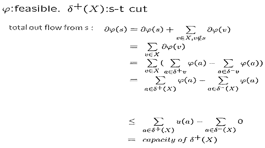
Maximum-flow Minimum-cut Theorem(最大流-最小カットの定理)では、可能流の最も小さいカットを最小カットとする。

Ford Fulkerson(1956)が発表したMaximum-flow minimum-cut Theoremとして、

を用いても良い。
この最小カットの検出のためのアルゴリズムはラべリング法をはじめとして、いくつか存在し、検出の高速化に寄与している。
第4実施形態は、MNA法と手続き型CKB法により第3問題点を解決している。
複数のQ-time制約の構造分析(MNA1法)と製造フロー全体の生産物流の解析(MNA2法)とに基づいて、製造フロー全体のQ-time制約区間を同時管理する方法(手続き型CKB法)を提案した。ここで、MNA法は、Manufacturing Network Analysisの略称で、MNA1法とMNA2法の総称をMNA法とした。第4実施形態では、これらの仕様書とプログラムフロー等を対象とする。
複数のQ-time制約の構造分析(MNA1法)と製造フロー全体の生産物流の解析(MNA2法)とに基づいて、製造フロー全体のQ-time制約区間を同時管理する方法(手続き型CKB法)を提案した。ここで、MNA法は、Manufacturing Network Analysisの略称で、MNA1法とMNA2法の総称をMNA法とした。第4実施形態では、これらの仕様書とプログラムフロー等を対象とする。
ここで、MNA1法は、複数のQ-time制約の構造分析、および同時管理の方法である。MNA2法は、動的なボトルネック箇所の検出・監視・予測のための解析方法である。手続き型CKB法は、MNA1法、MNA2法、およびCKB法を用いて、生産システム内の全てのQ-time制約を最適に同時管理する手続き方法である。
これら3つの方法により、製造フローの全体の生産流量に合わせて各Q-time制約区間の分散管理を実現し、生産変動に実時間で対応できる計算の高速性と全体最適化の両方が達成できる。なお、MNA1法やMNA2法は、単独でも使用可能である。
これら3つの方法により、製造フローの全体の生産流量に合わせて各Q-time制約区間の分散管理を実現し、生産変動に実時間で対応できる計算の高速性と全体最適化の両方が達成できる。なお、MNA1法やMNA2法は、単独でも使用可能である。
次に、連動物流制御法(手続き型CKB法)の効果をシミュレーション実験によって確かめる。
[目的と方法]
今回のシミュレーション実験の目的は、複数のQ-time制約が存在する生産工程において、複数のQ-time制約が成す干渉構造を考慮せずに意図的な生産物流制御を行う非特許文献1に記載の方法の場合(以下、従来型Q-time制約区間管理ルールと呼ぶ)と、複数のQ-time制約が成す干渉構造を考慮して同時に管理する手続き型CKB法の性能を比較することで、手続き型CKB法の効果を確かめることにある。
実験方法には、図58に示した、5つの装置群、7つの処理工程、および5つのQ-time制約が設定された非特許文献1に記載の実工場の生産工程のモデルと設定条件を用いたシミュレーション実験を行う。このモデルでは、同一装置群が繰返し処理のために共用される。生産工程におけるトラフィックを非特許文献1と同様に設定し、ロットは定期到着およびポアソン到着としてシミュレーション実験を行った。
[目的と方法]
今回のシミュレーション実験の目的は、複数のQ-time制約が存在する生産工程において、複数のQ-time制約が成す干渉構造を考慮せずに意図的な生産物流制御を行う非特許文献1に記載の方法の場合(以下、従来型Q-time制約区間管理ルールと呼ぶ)と、複数のQ-time制約が成す干渉構造を考慮して同時に管理する手続き型CKB法の性能を比較することで、手続き型CKB法の効果を確かめることにある。
実験方法には、図58に示した、5つの装置群、7つの処理工程、および5つのQ-time制約が設定された非特許文献1に記載の実工場の生産工程のモデルと設定条件を用いたシミュレーション実験を行う。このモデルでは、同一装置群が繰返し処理のために共用される。生産工程におけるトラフィックを非特許文献1と同様に設定し、ロットは定期到着およびポアソン到着としてシミュレーション実験を行った。
シミュレーション実験の結果、図59に示す通り、手続き型CKB法は、非特許文献1に記載の従来型Q-time制約区間管理ルールと比べて、生産率を向上しつつ工程間待ち時間を約60~80%短縮することを確かめた。
また、最適指標生成にかかる計算時間に関する性能評価結果から、非特許文献1で3秒を要していた計算時間を0.005秒程に抑え、600分の一の計算時間を実現することが確かめられた。なお、この性能評価は、同程度性能以下の計算機(パーソナルコンピューター)を用いて実験した結果である。
また、最適指標生成にかかる計算時間に関する性能評価結果から、非特許文献1で3秒を要していた計算時間を0.005秒程に抑え、600分の一の計算時間を実現することが確かめられた。なお、この性能評価は、同程度性能以下の計算機(パーソナルコンピューター)を用いて実験した結果である。
<第5実施形態>
[第2実施形態での問題点と課題]
第2実施形態では、図64に示すような段取り時間による保全時期のずれやその影響を考慮していない点に問題があった。また、半導体製造における段取り時間は、生産期間のうち4分の1を占める重要な管理対象であり、最大の非生産期間である段取り時間を低減する方法を提供する課題が残されていた。第5実施形態は、第2実施形態の変形例で、段取り業務最小化法を保全管理法と統合した装置業務管理法により問題・課題を解決している。半導体製造の生産工程における生産期間の4分の1を占める製造装置の段取り時間を低減し、また逆手に活用する特徴を持つ。本実施形態では、装置業務管理法(以下、JAMP-wS法という)について説明する。
[第2実施形態での問題点と課題]
第2実施形態では、図64に示すような段取り時間による保全時期のずれやその影響を考慮していない点に問題があった。また、半導体製造における段取り時間は、生産期間のうち4分の1を占める重要な管理対象であり、最大の非生産期間である段取り時間を低減する方法を提供する課題が残されていた。第5実施形態は、第2実施形態の変形例で、段取り業務最小化法を保全管理法と統合した装置業務管理法により問題・課題を解決している。半導体製造の生産工程における生産期間の4分の1を占める製造装置の段取り時間を低減し、また逆手に活用する特徴を持つ。本実施形態では、装置業務管理法(以下、JAMP-wS法という)について説明する。
図60を参照して、本発明の第5実施形態に係る最適指標生成装置について説明する。
本発明の第5実施形態に係る最適指標生成装置51は、例えば、装置の保全や多品種生産におけるプロセス切り替えのための段取りなど製造エンジニアリング業務の運用方法について、生産工程#1にそれぞれ設けられた装置群5に関わるエンジニアリング業務のスケジュール等を管理する生産管理システム10を制御の対象としている。同時に、製造装置の予防保全や段取りの時期を適正化する運用方法ついて、生産工程#2にそれぞれ設けられた装置群5の装置関連業務の計画や指示や実績を管理する生産管理システム10やエンジニアリング業務システム29を制御の対象としている。
本発明の第5実施形態に係る最適指標生成装置51は、例えば、装置の保全や多品種生産におけるプロセス切り替えのための段取りなど製造エンジニアリング業務の運用方法について、生産工程#1にそれぞれ設けられた装置群5に関わるエンジニアリング業務のスケジュール等を管理する生産管理システム10を制御の対象としている。同時に、製造装置の予防保全や段取りの時期を適正化する運用方法ついて、生産工程#2にそれぞれ設けられた装置群5の装置関連業務の計画や指示や実績を管理する生産管理システム10やエンジニアリング業務システム29を制御の対象としている。
図60に示すように、最適指標生成装置51は、図1に示す最適指標生成装置11(第1実施形態)と同様に、入力部12、Q-time構造分析部14、を備えている。また、図30に示す最適指標生成装置21(第2実施形態)と同様に、入力部22、補助入力部23、を備えている。第1実施形態や第2実施形態と比較して、第5実施形態に特徴的な構成は、図60に示すように、補助入力部(JAMP-wS法)52、段取り替えサイクル算定部53、装置区分算定部54、JAMP-wS最適論理値計算部55、感度解析部(JAMP特性)58、開始終了時期算出部56、感度解析部(性能特性)57、を備えていることにある。
ここで、第5実施形態に特徴的な上記構成について説明する。
補助入力部(JAMP-wS法)52は、装置使用可能品種/スペック対応、多品種・繰返し処理における段取り替え時間、段取り活用方法(3種類ほかから選択)、装置-品種スペック割当ルール(3種類ほかから選択)、装置-品種割当(固有条件)、多品種仕掛り、などの情報を入力する。
段取り活用方法の設定によって、最適理論値計算部55における計算結果が変わる。段取り活用方法は、不可避な段取り時間の活用方法を規定するもので、例えば、JAMP法における保全時期分散化率を高める目的、保全時間の長大化に対応する余裕時間を配置する目的、およびそれら両方を融合した目的、などがある。最適指標生成装置51のユーザーが選択した段取り活用ルールを、補助入力部(JAMP-wS法)52から入力する。
補助入力部(JAMP-wS法)52は、装置使用可能品種/スペック対応、多品種・繰返し処理における段取り替え時間、段取り活用方法(3種類ほかから選択)、装置-品種スペック割当ルール(3種類ほかから選択)、装置-品種割当(固有条件)、多品種仕掛り、などの情報を入力する。
段取り活用方法の設定によって、最適理論値計算部55における計算結果が変わる。段取り活用方法は、不可避な段取り時間の活用方法を規定するもので、例えば、JAMP法における保全時期分散化率を高める目的、保全時間の長大化に対応する余裕時間を配置する目的、およびそれら両方を融合した目的、などがある。最適指標生成装置51のユーザーが選択した段取り活用ルールを、補助入力部(JAMP-wS法)52から入力する。
段取り替えサイクル算定部53は、生産工程#1のQ-time制約や工程納期を遵守しつつ、装置群5の段取り率が最小になる多品種生産順序(以下、生産サイクル)と生産周期を算定する。段取り替えサイクル算定部53は、図62に示す手続き処理((0)装置-品種割当て決定、(1)多品種生産サイクル検出部、(2)多品種生産周期算定部、(3)最小段取りサイクル算定部)を行う。(0)では、補助入力部52から固有の装置-品種割当て情報が入力された場合は、入力された情報を使う。
装置区分算定部54は、各入力部と段取り替えサイクル算定部53の算定結果とを入力として、JAMP-wS最適論理値計算部55の計算結果と装置実体とを対応付けるための情報を算定する。装置区分算定部54は、図63に示す手続き処理((1)装置区分別必要台数算出、(2)段取り時間順ソート、(3)装置区分と保全順序の決定)を行う。
JAMP-wS最適論理値計算部55は、入力部22と補助入力部23と補助入力部52、および段取り替えサイクル算定部53と装置区分算定部54の算出結果を入力として、装置群5の装置の保全時期の分散化を図り、装置群5が常に高い処理能力を維持するための各装置の保全時期および各期の装置群の生産能力を算出する。例えば、常用装置と代替装置とに関する保全の開始・終了時期、各装置の多品種生産サイクル、段取り周期などの情報を算出し、生産管理システム10やエンジニアリング業務システム29に供給する。
開始終了時期算出部56は、JAMP-wS最適論理値計算部55の算出結果を内部記憶部56aに記憶する。また、開始終了時期算出部56は、内部記憶部56aと生産管理システム10やエンジニアリング業務システム29の生産実績や装置関連業務実績の情報を照合して、生産管理システム10における生産指示やエンジニアリング業務システム29における業務指示のための情報を出力する。これら生産指示や業務指示のそれぞれに固有の識別番号等が付され、生産実績や業務実績と内部記憶部56aとの照合に利用することができる。
開始終了時期算出部56では、第2実施形態の開始終了時期算出部26とは異なり、保全に加えて段取り業務の情報が追加されている。
開始終了時期算出部56では、第2実施形態の開始終了時期算出部26とは異なり、保全に加えて段取り業務の情報が追加されている。
感度解析部(性能特性)57は、JAMP-wS法に使用した入力データ、JAMP-wS法最適理論値の条件を入力し、決定されたJAMP-wS法最適理論値の条件の下で、生産工程の性能評価のための計算を行い、性能特性として、装置群の処理能力や生産負荷(仕掛り到着率)に対する各種性能評価指標を生産管理システム10や装置エンジニアリング業務システムに出力する。
感度解析部(JAMP-wS特性)58は、JAMP最適論理値計算部55から入力されるJAMP-wS法理論値計算結果、各装置の処理負荷(回数)や段取り周期とその時期が変動した場合のJAMP法理論値計算の結果の変化特性を算定する。また、感度解析部((JAMP-wS特性)58は、この感度解析結果を、内部記憶部58aに記録しておき、JAMP法理論値計算結果、各装置の処理負荷(回数)とその処理時期が動的に変化した場合に、即時に更新データとして使用することもできる。内部記憶部58aの情報は、最適指標生成装置51の実行必要性の判定にも用いられる。この必要性の判定は、管理対象の生産工程#1における各種の変動(装置群の処理能力の変化や、目標生産率の変更、トラフィックの変動など)に対応して判断される。必要性が確認された場合、最適指標生成装置51に計算指示が出される。
図60と図61を参照して、本発明の第5実施形態に係る最適指標生成装置51の動作について説明する。
ステップS51では、Q-time制約に関する情報を生産管理システム10を介して入力部12により入力する。ステップS52では、Q-time構造分析部43を経て算出した情報と、生産実行システムに含まれる複数の装置に関する情報を生産管理システム10を介して入力部22と補助入力部23により入力する。
さらに、ステップS53では、装置の段取り替えや段取り活用方法に関する情報を補助入力部52から入力した情報を用いて、段取り替えサイクル算定部53により、Q-time制約や工程納期を遵守しつつ各装置の段取り率最小となる多品種生産サイクルおよび段取り周期等を算出し、装置区分算定部54に入力する。
次に、ステップS54では、装置区分算定部54により複数の装置を常用能力を有する常用装置と代替能力を有する代替装置とに区分する。ステップS55では、装置能力区分と入力された情報および各装置の段取り情報からJAMP-wS最適論理値計算部55により複数の常用装置と代替装置(および常用能力と代替能力)に対する生産負荷・稼働回数と稼働時期を算出する。
ステップS56では、常用装置と代替装置とに関する予防保全開始・終了時期および各装置の段取り周期や品種生産サイクルを開始終了時期算出部56により算出すると共に内部記憶56aに記憶する。
ステップS57では、開始終了時期算出部56により算出された製品処理・段取り・保全の最適な開始終了時期情報を生産管理システム10やエンジニアリング業務システム29に供給する。
これら生産や業務の最適な開始終了時期情報それぞれに固有の識別番号等が付され、生産管理システム10やエンジニアリング業務システム29で管理される生産実績や業務実績と内部記憶部56aとの照合に利用することができる。
ステップS51では、Q-time制約に関する情報を生産管理システム10を介して入力部12により入力する。ステップS52では、Q-time構造分析部43を経て算出した情報と、生産実行システムに含まれる複数の装置に関する情報を生産管理システム10を介して入力部22と補助入力部23により入力する。
さらに、ステップS53では、装置の段取り替えや段取り活用方法に関する情報を補助入力部52から入力した情報を用いて、段取り替えサイクル算定部53により、Q-time制約や工程納期を遵守しつつ各装置の段取り率最小となる多品種生産サイクルおよび段取り周期等を算出し、装置区分算定部54に入力する。
次に、ステップS54では、装置区分算定部54により複数の装置を常用能力を有する常用装置と代替能力を有する代替装置とに区分する。ステップS55では、装置能力区分と入力された情報および各装置の段取り情報からJAMP-wS最適論理値計算部55により複数の常用装置と代替装置(および常用能力と代替能力)に対する生産負荷・稼働回数と稼働時期を算出する。
ステップS56では、常用装置と代替装置とに関する予防保全開始・終了時期および各装置の段取り周期や品種生産サイクルを開始終了時期算出部56により算出すると共に内部記憶56aに記憶する。
ステップS57では、開始終了時期算出部56により算出された製品処理・段取り・保全の最適な開始終了時期情報を生産管理システム10やエンジニアリング業務システム29に供給する。
これら生産や業務の最適な開始終了時期情報それぞれに固有の識別番号等が付され、生産管理システム10やエンジニアリング業務システム29で管理される生産実績や業務実績と内部記憶部56aとの照合に利用することができる。
図60の段取り替えサイクル算定部53は、図62に示す処理フローに従って算定を行う。段取り替えサイクル算定部53の計算手続きは、(S61)装置-品種割当て決定、(S62)多品種生産サイクル検出、(S63)多品種生産周期算定、(S64)最小段取りサイクル算定、の4段階で構成される。
まず、ステップS61では、段取り替えサイクル算定の前処理で、補助入力部52から固有の割当て情報が入力された場合は、入力された情報を使う。固有の割当てが指定されない場合は、補助入力部(JAMP-wS法)52から入力された装置-品種割当ルールと装置使用可能品種/スペック対応に従って品種-装置割当を算定する。装置-品種割当ルールでは、ある品種の生産率が一定期間に渡って大幅に減少するまたはゼロになる生産リスクと段取り時間の低減とが考慮される。
次に、ステップS62では、多品種生産サイクル検出では、装置を共用するn品種に対する(n-1)!個の生産サイクルを抽出し、各サイクルについて、其々の段取り替えが1回ずつ行われる1周期における総段取り時間を算定する。
次に、ステップS63では、多品種生産周期算定では、ステップS62で抽出した生産サイクル毎に、多品種ロットのQ-time制約を遵守しつつ段取りを最小化する生産周期を算定する。最後に、多品種生産周期算定と1周期における段取り時間から、最小段取り率サイクルを算定する。
ステップS64では、段取り替えサイクル算定部53では、3品種以上の生産ロットに共用される製造装置において、Q-time制約等の滞在時間制約を遵守しつつ段取りを最小化することを可能にしている。
まず、ステップS61では、段取り替えサイクル算定の前処理で、補助入力部52から固有の割当て情報が入力された場合は、入力された情報を使う。固有の割当てが指定されない場合は、補助入力部(JAMP-wS法)52から入力された装置-品種割当ルールと装置使用可能品種/スペック対応に従って品種-装置割当を算定する。装置-品種割当ルールでは、ある品種の生産率が一定期間に渡って大幅に減少するまたはゼロになる生産リスクと段取り時間の低減とが考慮される。
次に、ステップS62では、多品種生産サイクル検出では、装置を共用するn品種に対する(n-1)!個の生産サイクルを抽出し、各サイクルについて、其々の段取り替えが1回ずつ行われる1周期における総段取り時間を算定する。
次に、ステップS63では、多品種生産周期算定では、ステップS62で抽出した生産サイクル毎に、多品種ロットのQ-time制約を遵守しつつ段取りを最小化する生産周期を算定する。最後に、多品種生産周期算定と1周期における段取り時間から、最小段取り率サイクルを算定する。
ステップS64では、段取り替えサイクル算定部53では、3品種以上の生産ロットに共用される製造装置において、Q-time制約等の滞在時間制約を遵守しつつ段取りを最小化することを可能にしている。
図60の装置区分算定部54は、図63に示す処理フローに従って算定を行う。
装置区分算定部54の手続きは、(S71)装置区分別必要台数算出→(S72)段取り順ソート→(S73)装置区分と保全順序決定、の3段階で構成される。まず、(S71)装置区分別必要台数算出では、第2実施形態と同様に、常用装置(常用能力)と代替装置(代替能力)の区分別の数量を算定する。(S72)段取り順ソートでは、生産工程#1の装置群5に属する各装置について、段取り替えサイクル算定部53で算定された段取り率の大小順に並べ替える。(S73)装置区分と保全順序決定で、(S72)段取り順ソートの結果に基づき、各装置の装置区分と保全順序を決定する。
装置区分算定部54の手続きは、(S71)装置区分別必要台数算出→(S72)段取り順ソート→(S73)装置区分と保全順序決定、の3段階で構成される。まず、(S71)装置区分別必要台数算出では、第2実施形態と同様に、常用装置(常用能力)と代替装置(代替能力)の区分別の数量を算定する。(S72)段取り順ソートでは、生産工程#1の装置群5に属する各装置について、段取り替えサイクル算定部53で算定された段取り率の大小順に並べ替える。(S73)装置区分と保全順序決定で、(S72)段取り順ソートの結果に基づき、各装置の装置区分と保全順序を決定する。
段取り替えサイクル算定部53の算定手続きで、(S61)装置-品種割当て決定において、補助入力部(JAMP-wS法)52から固有の割当てが指定されない場合は、補助入力部(JAMP-wS法)52から入力された装置-品種割当ルールと装置使用可能品種/スペック対応に従って品種-装置割当を算定する。装置-品種割当ルールでは、ある品種の生産率が一定期間に渡って大幅に減少するまたはゼロになるような生産リスクと段取り時間の低減とが考慮される。例えば、(A)段取り最小化ルール、(C)生産リスク最小化ルール、および、(B)段取り-生産リスク調整型ルールの3種類などを備えている。(A)段取り最小化ルールは、段取りを最小化するために、生産負荷とサービス率から各品種の必要装置台数を算定し、その整数台は可能な限り専用装置に割り当て、残り端数分を複数品種の共用装置に割り当てる。(C)生産リスク最小化ルールは、生産リスクを最小化するために、各製品品種の使用可能装置に均等に生産負荷を配分する方法で、装置側から見ると、同一装置において複数の製品品種を処理する割り当てとなる。(B)段取り-生産リスク調整型ルールは、(A)段取り最小化ルールと(C)生産リスク最小化ルールの中庸に位置するルールで、過去の実績データを元に、ある程度の共用装置と専用装置を組み合わせた割り当てを行うものである。各品種の生産負荷と装置一台当たりの平均負荷から、必要な装置台数を計算し、その台数に所定の(例えば、プラス1台)のマージンを追加する。なお、(S61)装置-品種割当て決定の機能を単体で使用することもできる。
図62に示した段取り替えサイクル算定部53の算定フロー上の(2)多品種生産周期算定では、図65に示すように工程滞在時間制約を満たす仕掛上限値を算定し、次に各品種ロットの仕掛上限値を満たすように、図67に示すような生産周期を算定する。まず、図65に示す仕掛上限値を、待ち行列理論のリトルの公式を応用して数式38から数式32により算定する。
連続生産期間Tp、待ち時間Tw、製品ロット到着率λ0、製品サービス率μ、生産周期Tc、基本割当装置台数nとすると、ある品種の仕掛品のバッファ内での平均滞在時間WBは、数式38で表せる。
連続生産期間Tp、待ち時間Tw、製品ロット到着率λ0、製品サービス率μ、生産周期Tc、基本割当装置台数nとすると、ある品種の仕掛品のバッファ内での平均滞在時間WBは、数式38で表せる。
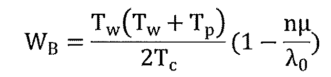
で表せる。ここで、バッファに蓄積されることになる仕掛品の最大量とこの時の待ち時間上限時間(平均)は、それぞれ、

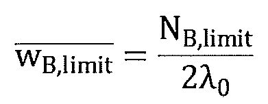
と表せる。

(i≠j)、は制約条件で、

は、k種類の品種交換に必要とされる時間の総和である。
下数式43~47で定式化した最大化問題を解き、最大サイクルTcを求める。
最適化問題の定式化(例えば、図66に示すように3品種で生産順序がA、B、Cの場合)
最適化問題の定式化(例えば、図66に示すように3品種で生産順序がA、B、Cの場合)

ここで、A品種の処理後のアイドル時間、B品種の処理後のアイドル時間、C品種の処理後のアイドル時間(スラック)をそれぞれをtA、tB、tCとすると、
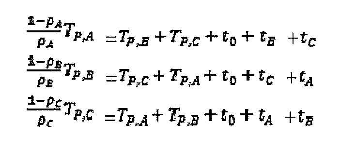
改めて、

であるから

ここで、

制約条件下で、Tcの最大生産周期を算定する。
3品種以上の場合には、全2通りの品種サイクルに対する最大サイクルを求める。
ここで、段取りを要する処理スペックの違いは、製品品種によるものに限らない。繰返し処理の場合でも段取りが発生する場合には、スペック(製品品種・繰返し処理段階や処理条件等の対)の別で、段取り最小化サイクルを求める。ここで、繰返し処理ロットにおける円滑な生産物流を実現しスループットを最大化するためには、繰返し処理ロットに対するサービス率が均等になるように配分すればよい。
段取り替えサイクル算定部53の処理フロー上の(3)最小段取りサイクル算定部では、図67に示すように、各サイクルのk種類の品種交換に必要とされる時間の総和t0を、各品種サイクルのTcで割り、段取り率を算定する。この段取り率が最小の生産サイクルと生産周期を採用する。
JAMP-wS最適論理値計算部55は、入力部22、補助入力部23、および段取り替えサイクル算定部53、装置区分算定部54から入力される情報に基づいて、JAMP-wS法理論値計算の結果、各装置の処理負荷(回数)とその処理時期、生産サイクルと段取り時期、および保全時期などを算出して出力する。
感度解析部(JAMP-wS特性)58は、JAMP-wS最適論理値計算部55から入力される処理負荷(回数)とその処理時期、生産サイクルや段取り時間、保全時間、が変動した場合のJAMP-wS法理論値計算の結果の変化特性を算定する。感度解析部(JAMP-wS特性)58は、この感度解析結果を、内部記憶部58aに記録しておき、JAMP-wS法理論値計算結果、各装置の処理負荷(回数)とその処理時期、生産サイクルや段取り時間、保全時間が動的に変化した場合に、即時に更新データとして使用することもできる。内部記憶部58aの情報は、最適指標生成51の実行必要性の判定にも用いられる。この必要性の判定は、管理対象の生産工程#1における各種の変動(装置群の処理能力の変化や、目標生産率の変更、トラフィックの変動など)に対応して判断される。必要性が確認された場合、最適指標生成51に計算指示が出される。
感度解析部(JAMP-wS特性)58は、JAMP-wS最適論理値計算部55から入力される処理負荷(回数)とその処理時期、生産サイクルや段取り時間、保全時間、が変動した場合のJAMP-wS法理論値計算の結果の変化特性を算定する。感度解析部(JAMP-wS特性)58は、この感度解析結果を、内部記憶部58aに記録しておき、JAMP-wS法理論値計算結果、各装置の処理負荷(回数)とその処理時期、生産サイクルや段取り時間、保全時間が動的に変化した場合に、即時に更新データとして使用することもできる。内部記憶部58aの情報は、最適指標生成51の実行必要性の判定にも用いられる。この必要性の判定は、管理対象の生産工程#1における各種の変動(装置群の処理能力の変化や、目標生産率の変更、トラフィックの変動など)に対応して判断される。必要性が確認された場合、最適指標生成51に計算指示が出される。
JAMP-wS最適論理値計算部55では、第2実施形態のJAMP最適論理値計算部24での計算とは異なり、多品種生産における段取り時間による可動時間長のズレや常用装置から代替装置に移行する代替処理回数の変化を考慮する。例えば、常用装置j(j=1、…、m’)とするとき、装置jの可動期間における段取り時間の総和がそれぞれTs(j)であれば、装置jの連続稼働期間は段取り時間Ts(j)の分後ろにずれる。また、常用装置を保全順序順に並べた際の装置番号をjとするとき、常用装置jのJAMP法計算における必要代替回数は、

となる。ここで、

の場合、負になるため代替回数の軽減が可能になる。これは、即ち、段取り時間を逆手に活用することによって、保全時期の分散化の可能性を高められることを意味する。常用装置m’台全体としては代替処理個数は、段取りを活用することにより、
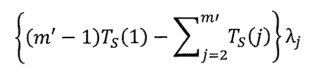
回減らすことが可能となる。これを利用して、図69に示す段取り活用法(1)を定めた。また、一方で、実際の工場では、保全時間が予定より長大化することが少なくない。JAMP法が提供する保全時期分散化方法は、ある保全が終了した後に次の保全が開始するまでの時間間隔をゼロから可能な範囲まで代替回数や段取り時間を用いて柔軟に調整できる。そこで、保全時間の長大化へ対応するために段取り時間を活用する図69に示す段取り活用(2)を定めた。段取り活用法(3)は、段取り活用方法(1)と段取り活用法(2)を合体させたものである。
となる。ここで、
の場合、負になるため代替回数の軽減が可能になる。これは、即ち、段取り時間を逆手に活用することによって、保全時期の分散化の可能性を高められることを意味する。常用装置m’台全体としては代替処理個数は、段取りを活用することにより、
回減らすことが可能となる。これを利用して、図69に示す段取り活用法(1)を定めた。また、一方で、実際の工場では、保全時間が予定より長大化することが少なくない。JAMP法が提供する保全時期分散化方法は、ある保全が終了した後に次の保全が開始するまでの時間間隔をゼロから可能な範囲まで代替回数や段取り時間を用いて柔軟に調整できる。そこで、保全時間の長大化へ対応するために段取り時間を活用する図69に示す段取り活用(2)を定めた。段取り活用法(3)は、段取り活用方法(1)と段取り活用法(2)を合体させたものである。
第5実施形態では、第2実施形態とは異なり、図64に示すような段取り時間による保全時期のずれやその影響を考慮すると共に、図69に示したように不可避な段取り時間を活用する方法を提供する。生産工程における生産期間のうち4分の1を占める段取り時間を低減し、また逆手に活用して、装置の稼動時間や生産能力の低下を抑制する特徴を持つ。
次に、JAMP-wS法の効果を数値実験によって確かめる。
[目的と方法]
図17(Q-time制約区間)に示した実際の生産工程モデルを用いて、典型的ルール(先着順(FCFS))や、Q-time制約区間投入制御付き先着順(以下、FCFS-CT)、投入制御付き最短処理時間順(以下、SPT-CT)などの従来法と、本発明の段取り低減・活用方法の性能を比較する。性能指標には、単位生産期間あたりの段取り時間の占める割合として定義される段取り率、生産ロット投入率と工程の良品出力率の比を表す良品生産率、ならびに、良品生産率と稼動率の総合的指標である総合設備効率(以下OEE)を用いた。総合設備効率は、実用上重要な性能指標で、半導体製造等のように製造コストに占める設備の減価償却費が非常に高い産業において重要視されている。なお、ここでは、Q-time制約を遵守した非リワークロットを良品とした。また、先行技術(非特許文献1や非特許文献2など)との計算時間の比較を行う。
[目的と方法]
図17(Q-time制約区間)に示した実際の生産工程モデルを用いて、典型的ルール(先着順(FCFS))や、Q-time制約区間投入制御付き先着順(以下、FCFS-CT)、投入制御付き最短処理時間順(以下、SPT-CT)などの従来法と、本発明の段取り低減・活用方法の性能を比較する。性能指標には、単位生産期間あたりの段取り時間の占める割合として定義される段取り率、生産ロット投入率と工程の良品出力率の比を表す良品生産率、ならびに、良品生産率と稼動率の総合的指標である総合設備効率(以下OEE)を用いた。総合設備効率は、実用上重要な性能指標で、半導体製造等のように製造コストに占める設備の減価償却費が非常に高い産業において重要視されている。なお、ここでは、Q-time制約を遵守した非リワークロットを良品とした。また、先行技術(非特許文献1や非特許文献2など)との計算時間の比較を行う。
性能評価の結果を図70と図71に示す。図70には、平均トラフィック強度が0.8の設定下の(あ)段取り率の比較と(い)良品生産率の比較結果を示す。これらの結果から、本発明の段取り低減方法が他の方法より大幅に段取りを低減し、かつ、唯一全ての品種の目標生産率を達成することが確かめられた。SPT-CTでは品種間の生産率の格差が大きく、FCFS-CTでは段取り率が高い。また、Q-time制約区間に対する投入制御を付けないFCFSでは、著しく良品率が低くなる。
図71に示す通り、本発明の提案手法が、総合設備効率(OEE)を高められる方法であることが確かめられた。
計算時間に関しては、非特許文献1で3秒を要していた計算を0.01秒以内に抑え、つまり300分の1の計算時間を実現した。これにより、保全等を含むまとまった生産期間を対象にした生産業務やエンジニアリング業務の実時間での最適管理を実現できる(実工場では、実時間管理のために各生産指示を約3秒以内に高速行えることが期待されている)。また、非特許文献1や非特許文献2に応用されている混合整数計画法の計算オーダーが指数時間に従うのに対して、本発明の第5実施形態の計算オーダーは線形時間を実現する方法であり、計算の高速性を実現している。例えば、非特許文献1の計算では、対象とする生産工程の一部(5装置群7工程)について生産期間10時間分の生産スケジュールの計算に3秒かかり、その計算時間は指数時間に従うことから原理的に6日以上の計算を6日以内に終えることが難しい。しかし、本発明の第5実施形態の方法では、数カ月の生産期間を対象にした生産業務とエンジニアリング業務の計画を数秒以内に計算することを可能にしている。こうして、現実に生じる動的な変化に対応するための再計算を即時に行う性能も実現している。
図71に示す通り、本発明の提案手法が、総合設備効率(OEE)を高められる方法であることが確かめられた。
計算時間に関しては、非特許文献1で3秒を要していた計算を0.01秒以内に抑え、つまり300分の1の計算時間を実現した。これにより、保全等を含むまとまった生産期間を対象にした生産業務やエンジニアリング業務の実時間での最適管理を実現できる(実工場では、実時間管理のために各生産指示を約3秒以内に高速行えることが期待されている)。また、非特許文献1や非特許文献2に応用されている混合整数計画法の計算オーダーが指数時間に従うのに対して、本発明の第5実施形態の計算オーダーは線形時間を実現する方法であり、計算の高速性を実現している。例えば、非特許文献1の計算では、対象とする生産工程の一部(5装置群7工程)について生産期間10時間分の生産スケジュールの計算に3秒かかり、その計算時間は指数時間に従うことから原理的に6日以上の計算を6日以内に終えることが難しい。しかし、本発明の第5実施形態の方法では、数カ月の生産期間を対象にした生産業務とエンジニアリング業務の計画を数秒以内に計算することを可能にしている。こうして、現実に生じる動的な変化に対応するための再計算を即時に行う性能も実現している。
第5実施形態は、第2実施形態の応用例で、段取り業務最小化法を保全管理法と統合した装置業務管理法により、Q-time制約など時間的制約を満たしつつ生産工程における製造装置の段取り時間を最小化し、段取り時間による保全時期のずれを考慮して保全時期を最適化する課題を解決している。半導体製造の生産工程における生産期間の4分の1を占める製造装置の段取り時間を低減し、また逆手に活用する特徴を持つ。典型的手法や従来技術と比べて、大幅に段取り時間を低減して生産設備の稼動率を高め、多品種生産における各品種の良品生産率を高められることが、性能評価実験により示された。
特に、フォトリソグラフィー装置群は、単価が高額で台数が限られており、生産工程全体の生産率を決定づけるボトルネックとなっている。また、フォトリソグラフィー工程では、マスク(工場ではレチクルと呼ばれる)という集積回路製造の原版を複数の装置で共有し、その交換のための段取り時間などが生産率に影響している。このようなボトルネックの生産率を高め、生産工程における製造装置の生産率を抜本的に向上し、また適切な多品種生産における段取り作業の最小化に基づく、適切なレチクル枚数の削減などのコスト削減の問題の解決に資するものである。
特に、フォトリソグラフィー装置群は、単価が高額で台数が限られており、生産工程全体の生産率を決定づけるボトルネックとなっている。また、フォトリソグラフィー工程では、マスク(工場ではレチクルと呼ばれる)という集積回路製造の原版を複数の装置で共有し、その交換のための段取り時間などが生産率に影響している。このようなボトルネックの生産率を高め、生産工程における製造装置の生産率を抜本的に向上し、また適切な多品種生産における段取り作業の最小化に基づく、適切なレチクル枚数の削減などのコスト削減の問題の解決に資するものである。
なお、本発明の第5実施形態に係る最適指標生成装置の変形例として、図61、図62、図63にあるフローチャートで示すプログラムをサーバに設けられたプロセッサに実行させてもよい。この変形例であっては、サーバに通信制御部を設け、通信制御部が生産管理システムやエンジニアリング業務システムと通信回線を介して情報を通信することとする。これにより、多品種の製品を生産するため複数の装置を制御する生産管理システムやエンジニアリング業務システムに対して、サーバが通信回線を介して複数の装置と製品に関する指標情報を送信することができる。
<第6実施形態>
[第3実施形態と第5実施形態での問題点と課題]
第3実施形態では、滞在時間に制約が付された生産工程における生産物流・在庫管理と製造設備の保全業務の最適化方法とを統合的に管理する方法を示した。また、第5実施形態では、製造設備に関わる段取り業務と保全業務を統合的に最適化する方法を示した。しかし、製造設備に関わる業務の統合的最適化方法と生産物流・在庫の最適管理方法を総合的に管理する技術として統合されていない点が課題であった。また他方で、プロセスの高度化・自動化に伴う製造設備の予定外停止への対応もまた重要な問題であり、予定された保全や段取りに加えて、突発的な故障や予知保全などによる動的な装置停止による生産能力の低下なども考慮できるような技術の改良が求められる。そこで、第6実施形態では、第3実施形態と第5実施形態の変形例として
、段取り業務と全般的保全管理法を生産物流・在庫管理と統合した製造業務統合管理法を示し、これらの課題を解決する方法を示す。
これらを踏まえた第6実施形態の動的装置業務・生産物流の最適管理方法を、CKB=JAMP-with Setup and Stop(以下、CKB=JAMP-wS2)法と呼ぶ。
第6実施形態では、多品種・繰返し処理ロットのQ-time制約を遵守しつつ段取りや保全業務の実施時期を最適化し、装置稼動率の向上と良品率向上と目標生産達成率向上を同時に達成することを目的とする。
[第3実施形態と第5実施形態での問題点と課題]
第3実施形態では、滞在時間に制約が付された生産工程における生産物流・在庫管理と製造設備の保全業務の最適化方法とを統合的に管理する方法を示した。また、第5実施形態では、製造設備に関わる段取り業務と保全業務を統合的に最適化する方法を示した。しかし、製造設備に関わる業務の統合的最適化方法と生産物流・在庫の最適管理方法を総合的に管理する技術として統合されていない点が課題であった。また他方で、プロセスの高度化・自動化に伴う製造設備の予定外停止への対応もまた重要な問題であり、予定された保全や段取りに加えて、突発的な故障や予知保全などによる動的な装置停止による生産能力の低下なども考慮できるような技術の改良が求められる。そこで、第6実施形態では、第3実施形態と第5実施形態の変形例として
、段取り業務と全般的保全管理法を生産物流・在庫管理と統合した製造業務統合管理法を示し、これらの課題を解決する方法を示す。
これらを踏まえた第6実施形態の動的装置業務・生産物流の最適管理方法を、CKB=JAMP-with Setup and Stop(以下、CKB=JAMP-wS2)法と呼ぶ。
第6実施形態では、多品種・繰返し処理ロットのQ-time制約を遵守しつつ段取りや保全業務の実施時期を最適化し、装置稼動率の向上と良品率向上と目標生産達成率向上を同時に達成することを目的とする。
図72を参照して、本発明の第6実施形態に係る最適指標生成装置61について説明する。本発明の第6実施形態に関わる最適指標生成装置61は、例えば、半導体を生産するための生産工程#1にそれぞれ設けられた処理工程(装置群)2および処理工程(装置群)3の生産スケジュールを管理する生産管理システム10を制御の対象としている。同時に、製造装置の予防保全や段取りの時期を適正化する運用方法、および、故障監視・予測に基づく事後保全・予知保全等を適正に管理する方法ついて、生産工程#2にそれぞれ設けられた装置群5の装置関連業務の計画や指示や実績を管理する生産管理システム10やエンジニアリング業務システム29、ならびに生産工程#1の業務を行うエンジニア/オペレータ、を制御の対象としている。
図72に示すように、最適指標生成装置61は、図48に示す最適指標生成装置31(第3実施形態)と同様に、入力部12、補助入力部13、Q-time構造分析部14、変動監視検出部32、入力変更検出部33、再計算必要性判断部34、を備えている。
また、最適指標生成装置61は、図60に示す最適指標生成装置51(第5実施形態)と同様に、入力部22、補助入力部(JAMP法)23、補助入力部(JAMP-wS法)52、段取り替えサイクル算定部53、装置区分算定部54、JAMP-wS最適論理値計算部55、感度解析部(JAMP-wS特性)58、など最適指標生成装置51の全体、を備えている。なお、図72では、入力部12と補助入力部13をまとめて入力モジュール(CKB法)12Aに、入力部22、補助入力部(JAMP法)23、補助入力部(JAMP-wS法)52をまとめて入力モジュール22Aとして表している。
第3および第5実施形態と比較して、第6実施形態に特徴的な構成は、図72に示すように、補助入力部(CKB=JAMP-wS2法)62、装置群生産周期位相設定部63、生産スパイク算定部64、CKB=JAMP-wS2最適理論値計算部65、指標算出部66、感度解析部(CKB=JAMP-wS2性能特性)67、感度解析部(CKB=JAMP-wS2特性)68、を備えていることにある。
また、最適指標生成装置61は、図60に示す最適指標生成装置51(第5実施形態)と同様に、入力部22、補助入力部(JAMP法)23、補助入力部(JAMP-wS法)52、段取り替えサイクル算定部53、装置区分算定部54、JAMP-wS最適論理値計算部55、感度解析部(JAMP-wS特性)58、など最適指標生成装置51の全体、を備えている。なお、図72では、入力部12と補助入力部13をまとめて入力モジュール(CKB法)12Aに、入力部22、補助入力部(JAMP法)23、補助入力部(JAMP-wS法)52をまとめて入力モジュール22Aとして表している。
第3および第5実施形態と比較して、第6実施形態に特徴的な構成は、図72に示すように、補助入力部(CKB=JAMP-wS2法)62、装置群生産周期位相設定部63、生産スパイク算定部64、CKB=JAMP-wS2最適理論値計算部65、指標算出部66、感度解析部(CKB=JAMP-wS2性能特性)67、感度解析部(CKB=JAMP-wS2特性)68、を備えていることにある。
第3実施形態や第5実施形態と対比させて、第6実施形態の主要な特徴を説明する。
第5実施形態では、予防保全時期の決定に際して、各装置で処理する多品種生産ロットのQ-time制約を遵守しつつ段取り時間の最小化を図り、さらに、不可避な段取り時間を逆手に活用して予防保全時期の分散化の進展や生産リスク提言を図る方法を示した。第5実施形態の最適指標生成装置51により、図75に示すような生産スパイクを可能な限り減じて、常に生産能力を高く維持することが可能となる。ここで、第5実施形態で算定された多品種生産の段取りや予防保全を考慮した各装置の生産負荷配分方法を用いることによって、第1実施形態、第3実施形態、ならびに第4実施形態に示した最適指標生成装置11、最適指標生成装置31、ならびに最適指標生成装置41の機能・性能を高める方法を第6実施形態で示す。第6実施形態では、製造設備の保全と多品種・繰返し生産の段取りを考慮してQ-time制約区間等の工程間滞在時間制限が付された生産工程を管理する方法を示す。
他方、最適指標生成装置31(第3実施形態)ほかでは、管理対象とする生産工程のボトルネックに合わせたQ-time制約区間の生産物流・在庫管理のための最適指標とその置き換え条件を生成した。第6実施形態では、第5実施形態の最適指標生成装置51で生成される保全や段取りや各装置への生産負荷配分に伴う各時点の装置群の生産能力や生産負荷の情報を元に、(1)ボトルネックの箇所や生産能力の変化を予期・分析し(生産スパイク算定部64)、第3実施形態や図49に示した生産スパイクの発生原因と分析方法を具体的に示し、Q-time制約区間の生産物流・在庫管理の応用例を具体化する(CKB=JAMP-wS2最適理論値計算部65)。(2)この時、最適指標生成装置51(第5実施形態)で算定される各装置の多品種生産サイクルに位相を導入することによって、生産工程の生産リスクを減じて生産率を高めるよう、生産スパイクを変形する(装置群生産周期位相設定部63)。
(3)また、第5実施形態で取り上げた予防保全や段取りや生産負荷配分に加えて、製造装置の異常の監視・予測に基づく予知保全や突発的な故障による生産スパイクの動的変化への対応方法についての記述を加える。
第5実施形態では、予防保全時期の決定に際して、各装置で処理する多品種生産ロットのQ-time制約を遵守しつつ段取り時間の最小化を図り、さらに、不可避な段取り時間を逆手に活用して予防保全時期の分散化の進展や生産リスク提言を図る方法を示した。第5実施形態の最適指標生成装置51により、図75に示すような生産スパイクを可能な限り減じて、常に生産能力を高く維持することが可能となる。ここで、第5実施形態で算定された多品種生産の段取りや予防保全を考慮した各装置の生産負荷配分方法を用いることによって、第1実施形態、第3実施形態、ならびに第4実施形態に示した最適指標生成装置11、最適指標生成装置31、ならびに最適指標生成装置41の機能・性能を高める方法を第6実施形態で示す。第6実施形態では、製造設備の保全と多品種・繰返し生産の段取りを考慮してQ-time制約区間等の工程間滞在時間制限が付された生産工程を管理する方法を示す。
他方、最適指標生成装置31(第3実施形態)ほかでは、管理対象とする生産工程のボトルネックに合わせたQ-time制約区間の生産物流・在庫管理のための最適指標とその置き換え条件を生成した。第6実施形態では、第5実施形態の最適指標生成装置51で生成される保全や段取りや各装置への生産負荷配分に伴う各時点の装置群の生産能力や生産負荷の情報を元に、(1)ボトルネックの箇所や生産能力の変化を予期・分析し(生産スパイク算定部64)、第3実施形態や図49に示した生産スパイクの発生原因と分析方法を具体的に示し、Q-time制約区間の生産物流・在庫管理の応用例を具体化する(CKB=JAMP-wS2最適理論値計算部65)。(2)この時、最適指標生成装置51(第5実施形態)で算定される各装置の多品種生産サイクルに位相を導入することによって、生産工程の生産リスクを減じて生産率を高めるよう、生産スパイクを変形する(装置群生産周期位相設定部63)。
(3)また、第5実施形態で取り上げた予防保全や段取りや生産負荷配分に加えて、製造装置の異常の監視・予測に基づく予知保全や突発的な故障による生産スパイクの動的変化への対応方法についての記述を加える。
図72と図73を参照して、本発明の第6実施形態に係る最適指標生成装置61の動作について説明する。
まず、第5実施形態の最適指標生成装置51の主要な処理を実行する。具体的には、ステップS81では、入力部12や補助入力部13を介して生産管理システム10やエンジニアリング業務システムから入力された情報に基づいてQ-time構造分析部43でQ-time構造を分析する。
ステップS82では、Q-time構造分析の結果と、入力部22や補助入力部(JAMP法)23や補助入力部(JAMP-wS法)52を介して生産管理システム10やエンジニアリング業務システムから入力された情報に基づいて、段取り替えサイクル算定部53、装置区分算定部54、JAMP-wS最適論理値計算部55の計算を実行する。
ステップS83では、JAMP-wS最適論理値計算部55の算出結果と感度解析部(JAMP-wS特性)58の算出結果が内部記憶58aに記憶される。
ステップS84では、JAMP-wS最適論理値計算部55から算出される複数の常用装置と代替装置(および常用能力と代替能力)の稼働回数と稼働時期、常用装置と代替装置とに関する予防保全開始・終了時期および各装置の段取り周期や品種生産サイクルを、開始終了時期算出部56を介して入力して、生産スパイク算定部64では、生産スパイクを算出し、内部記憶64aに記憶する。
ステップS85では、生産スパイク算定部64は、補助入力部(CKB=JAMP-wS2法)62と内部記憶64aから入力された情報を元に、感度解析部(JAMP-wS特性)58の内部記憶58aと照合して、動的な生産スパイクなどを算出し、内部記憶64aに記憶する。
また、ステップS86では、生産スパイク算定部64での計算に装置群生産周期位相設定部63の算定結果を用いて生産スパイクの変形することができる。
ステップS87、S88では、各入力部やQ-time構造分析部14や最適ロードルール判定部19ならびに生産スパイク算定部64から入力される情報に基づいて、CKB=JAMP-wS2最適理論値計算部65では、対象とする生産工程のQ-time制約区間における生産物流・在庫管理のための最適指標を生成し、生産管理システム10やエンジニアリング業務システム29、または生産工程#1のエンジニアやオペレータに指標算出部66を介して出力すると共に、内部記憶66aに記憶する。
また、ステップS89では、指標算出部66は、内部記憶部66aと生産管理システム10やエンジニアリング業務システム29などの生産実績や装置関連業務実績の情報を照合して、生産管理システム10における生産指示やエンジニアリング業務システム29における業務指示のための情報を出力する。これら生産指示や業務指示のそれぞれに固有の識別番号等が付され、生産実績や業務実績と内部記憶部66aとの照合に利用することができる。
指標算出部66では、第3実施形態の算出部17A、ならびに、第5実施形態の56と同様であるが、保全や段取り業務の情報と、生産物流・在庫管理に関する情報とが含まれた総合的な生産・業務指示情報を出力する点が異なる。
まず、第5実施形態の最適指標生成装置51の主要な処理を実行する。具体的には、ステップS81では、入力部12や補助入力部13を介して生産管理システム10やエンジニアリング業務システムから入力された情報に基づいてQ-time構造分析部43でQ-time構造を分析する。
ステップS82では、Q-time構造分析の結果と、入力部22や補助入力部(JAMP法)23や補助入力部(JAMP-wS法)52を介して生産管理システム10やエンジニアリング業務システムから入力された情報に基づいて、段取り替えサイクル算定部53、装置区分算定部54、JAMP-wS最適論理値計算部55の計算を実行する。
ステップS83では、JAMP-wS最適論理値計算部55の算出結果と感度解析部(JAMP-wS特性)58の算出結果が内部記憶58aに記憶される。
ステップS84では、JAMP-wS最適論理値計算部55から算出される複数の常用装置と代替装置(および常用能力と代替能力)の稼働回数と稼働時期、常用装置と代替装置とに関する予防保全開始・終了時期および各装置の段取り周期や品種生産サイクルを、開始終了時期算出部56を介して入力して、生産スパイク算定部64では、生産スパイクを算出し、内部記憶64aに記憶する。
ステップS85では、生産スパイク算定部64は、補助入力部(CKB=JAMP-wS2法)62と内部記憶64aから入力された情報を元に、感度解析部(JAMP-wS特性)58の内部記憶58aと照合して、動的な生産スパイクなどを算出し、内部記憶64aに記憶する。
また、ステップS86では、生産スパイク算定部64での計算に装置群生産周期位相設定部63の算定結果を用いて生産スパイクの変形することができる。
ステップS87、S88では、各入力部やQ-time構造分析部14や最適ロードルール判定部19ならびに生産スパイク算定部64から入力される情報に基づいて、CKB=JAMP-wS2最適理論値計算部65では、対象とする生産工程のQ-time制約区間における生産物流・在庫管理のための最適指標を生成し、生産管理システム10やエンジニアリング業務システム29、または生産工程#1のエンジニアやオペレータに指標算出部66を介して出力すると共に、内部記憶66aに記憶する。
また、ステップS89では、指標算出部66は、内部記憶部66aと生産管理システム10やエンジニアリング業務システム29などの生産実績や装置関連業務実績の情報を照合して、生産管理システム10における生産指示やエンジニアリング業務システム29における業務指示のための情報を出力する。これら生産指示や業務指示のそれぞれに固有の識別番号等が付され、生産実績や業務実績と内部記憶部66aとの照合に利用することができる。
指標算出部66では、第3実施形態の算出部17A、ならびに、第5実施形態の56と同様であるが、保全や段取り業務の情報と、生産物流・在庫管理に関する情報とが含まれた総合的な生産・業務指示情報を出力する点が異なる。
ここで、第6実施形態に特徴的な上記構成について説明する。
補助入力部62では、生産管理システム10やエンジニアリング業務システム29などを介して、動的な故障や予知保全の発生箇所や発生時期や保全終了予定時期、目標生産負荷(投入)計画の変更、生産工程の多品種ロットの仕掛り数量、などの情報を入力する。また、生産周期位相設定部63で用いる生産周期位相設定ルールに関する情報を入力する。
補助入力部62では、生産管理システム10やエンジニアリング業務システム29などを介して、動的な故障や予知保全の発生箇所や発生時期や保全終了予定時期、目標生産負荷(投入)計画の変更、生産工程の多品種ロットの仕掛り数量、などの情報を入力する。また、生産周期位相設定部63で用いる生産周期位相設定ルールに関する情報を入力する。
生産スパイク算定部64では、生産工程#1の装置群を対象として、図48の第3実施形態の最適指標生成装置31を用いた各装置群の生産能力の変化や補助入力部62の動的な生産能力または生産負荷の変動に関する情報を入力し、図74に示すような生産スパイクの大きさを分析する。生産スパイク算定部64では、算定した生産スパイクと生産スパイクによって発生する生産リスクに関わる情報を内部記憶64aに記憶する。
生産スパイクは、生産目標率や実績生産投入率に対する生産能力(装置群や工程のスループット)の差を示す。生産リスクとして、図75に示すような生産率(と在庫)に関する生産リスクと時間(と在庫)に関する生産リスクの2種類のリスクを分析する。
生産スパイクは、生産目標率や実績生産投入率に対する生産能力(装置群や工程のスループット)の差を示す。生産リスクとして、図75に示すような生産率(と在庫)に関する生産リスクと時間(と在庫)に関する生産リスクの2種類のリスクを分析する。
生産スパイク算定部64で算定される生産スパイクには、静的生産スパイクと、動的生産スパイクの2種類がある。静的生産スパイクには、各装置群のJAMP-wS法に基づく保全時期前・中・後の装置群の生産能力スパイク(最大生産率の時間推移)や、装置群の生産能力を多品種生産負荷に割付けた多品種生産負荷配分スパイク(ロット生産サイクルに基づく各品種の生産率の時間推移)、などを用いる。
また、補助入力部62から動的な故障や予知保全の情報入力を受けて、記憶部64aの生産スパイクを更新した場合の生産スパイクを、動的生産スパイクと呼ぶ。
生産スパイクの算定単位には、装置、装置群、複数装置群、処理工程、複数処理工程、などがある。
また、補助入力部62から動的な故障や予知保全の情報入力を受けて、記憶部64aの生産スパイクを更新した場合の生産スパイクを、動的生産スパイクと呼ぶ。
生産スパイクの算定単位には、装置、装置群、複数装置群、処理工程、複数処理工程、などがある。
生産スパイクを、図74に示す通り、目標生産率に対する生産能力の差として表現する。生産スパイクの大きさは、低下期のスパイクの深さと復旧期の長さによって定まるスパイクの面積で表す。生産スパイクの影響度合いは、スパイクの形状と大きさで決まる。
単一のスパイクに、複数個の異なる低下期や復旧期が重なることもある。このような生産スパイクは、例えば、段階的に保全対象装置台数が増えていった後、保全を終了した装置が段階的に製造処理を再開するような場合などに発現する他、図78のように複数工程のスパイクを重ねた複合スパイクに発現する。
単一のスパイクに、複数個の異なる低下期や復旧期が重なることもある。このような生産スパイクは、例えば、段階的に保全対象装置台数が増えていった後、保全を終了した装置が段階的に製造処理を再開するような場合などに発現する他、図78のように複数工程のスパイクを重ねた複合スパイクに発現する。
図74に示すような生産スパイク図を用いて、以下の手続きで解析し、図75に示すように生産スパイクと生産リスクを定量的に分析する。
(1)各装置群のJAMP-wS法に基づく算出結果を入力する
(2)各装置群jで予防保全、故障や予知保全などにより発生するスパイクk(低下期と復旧期)の深さと長さを算定する。
(A)低下期のスパイクの深さ(μ1(j,k)-μ2(j,k))と長さTr(j,k)によって定まる低下期終了点と目標生産率線(または生産工程の生産率容量など)の時間差:
(1)各装置群のJAMP-wS法に基づく算出結果を入力する
(2)各装置群jで予防保全、故障や予知保全などにより発生するスパイクk(低下期と復旧期)の深さと長さを算定する。
(A)低下期のスパイクの深さ(μ1(j,k)-μ2(j,k))と長さTr(j,k)によって定まる低下期終了点と目標生産率線(または生産工程の生産率容量など)の時間差:

(B)復旧期の長さ:

(C)生産スパイクの大きさ(=スパイクの面積):

この面積分が在庫ロスや生産期間ロスを引き起こす。これは、理想の生産能力や生産目標に対する生産実績の差を表し、各種生産目標割れの可能性(生産リスク)を定量化したものである。
(D)生産スパイクを用いた生産リスクの分析:
図74や図75に示すような生産スパイク図を用いて、生産リスクを以下(あ)と(い)の観点で定量的に分析する。
(あ)生産率(と在庫)に関する生産リスク:生産スパイクの面積
生産スパイクに与える目標生産率を、工程区間や生産工程全体のボトルネックにおける生産率とした場合、工程区間や生産工程全体の生産率を更に低下させる生産リスクを定量的に分析することができる。当該リスクの大きさSA(j,k)は、数式50で示した式で算定する。

(い)時間(と在庫)に関する生産リスク:限界線と実績の差分
対象とする装置群j、工程kにおける滞在時間の制約tdd(j,k)とtd(j,k)を比較してtdd(j,k)<td(j,k)である場合、滞在時間の制約を超過する生産リスクが発生する。この生産リスクの大きさを面積の差分SB(j,k)として計算する。
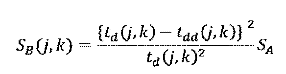
(3)(2)で算定された各装置群jで最大スパイクや生産リスクの大きな順に並べる。
(4)(2)で算定された各装置群jのスパイク(時刻tに依存)や生産リスクを重ね合わせ、図78に示すような生産工程を通した複合生産スパイクや複合生産リスクを算定する(Q-time制約区間、ボトルネック-ボトルネック区間、生産工程全体、など)。
なお、最適指標生成装置21(第2実施形態)の性能評価事例で図46に示したように、JAMP法を用いて保全時期を分散化(すなわち生産能力の平準化)を図ることによって生産スパイクが発生しない場合もある。このように、生産スパイク図は、最適指標生成装置の性能評価指標としても用いることができる。
装置群生産周期位相設定部63は、第5実施形態の最適指標生成装置61における段取り替えサイクル算定部53によって算定される各製造装置の多品種ロット生産サイクルに対して、多品種生産における生産スパイク・生産リスクを減ずる位相を算定する。装置群生産周期位相設定部63を用いることによって、生産スパイク・生産リスクを軽減することができる。
例えば、図22のような装置-品種割当がなされた装置群(処理工程)で、製品p1、p2、p3の3品種に共用される装置が3台(624、625、627)ある。これらの装置では、最適指標生成装置51(第5実施形態)を用いて、Q-time制約等の滞在時間制約を遵守しながら段取りを最小化する生産サイクルが算定される。例えば、p1、p2、p3の生産順序が最適と算定されたとする。ここで、3台が全て設定条件が同じのため最適生産順序もp1、p2、p3の同順で、其々の品種の継続可能生産時間がTp(p1)、Tp(p2)、Tp(p3)である場合、全ての装置で同一の生産サイクルを同じ生産サイクル開始点の設定下で用いると、最初のTp(p1)時間は、3台全てで品種p1を処理し、他の品種p2とp3の仕掛りロットはTp(p1)の時間待たされる。すると、このTp(p1)期間の品種p2とp3の処理工程では生産能力が低下し、生産スパイクや生産リスクが発生する可能性が高まる。このような事態を避け、全ての製品ロットに対して配分する生産能力を平準化するために、装置群生産周期位相設定部63を用いて、適切な位相を算定する。この位相の設定には、補助入力部62で入力される生産周期位相設定ルールを用いる。
例えば、図22のような装置-品種割当がなされた装置群(処理工程)で、製品p1、p2、p3の3品種に共用される装置が3台(624、625、627)ある。これらの装置では、最適指標生成装置51(第5実施形態)を用いて、Q-time制約等の滞在時間制約を遵守しながら段取りを最小化する生産サイクルが算定される。例えば、p1、p2、p3の生産順序が最適と算定されたとする。ここで、3台が全て設定条件が同じのため最適生産順序もp1、p2、p3の同順で、其々の品種の継続可能生産時間がTp(p1)、Tp(p2)、Tp(p3)である場合、全ての装置で同一の生産サイクルを同じ生産サイクル開始点の設定下で用いると、最初のTp(p1)時間は、3台全てで品種p1を処理し、他の品種p2とp3の仕掛りロットはTp(p1)の時間待たされる。すると、このTp(p1)期間の品種p2とp3の処理工程では生産能力が低下し、生産スパイクや生産リスクが発生する可能性が高まる。このような事態を避け、全ての製品ロットに対して配分する生産能力を平準化するために、装置群生産周期位相設定部63を用いて、適切な位相を算定する。この位相の設定には、補助入力部62で入力される生産周期位相設定ルールを用いる。
CKB=JAMP-wS2最適理論値計算部65は、最適指標生成装置51(第5実施形態)で算出された各装置における多品種生産の処理順序と段取りサイクル、処理負荷(回数)とその処理時期、装置群生産周期位相設定部63で設定された位相、および、所定サイクル分の装置群における処理能力の時間推移をもとに生産スパイク算定部64で算定された生産スパイクとを入力し、所定サイクル内で対象とする生産工程の処理能力や生産負荷(または生産目標)が切り替わる毎のCKB法最適理論値計算を行う。ここで、所定サイクルは、例えば、全ての常用装置が1回以上かつ全ての代替装置が1回ずつ予防保全を完了するまでの期間(1サイクル)、装置群の保全時期分散化の限界周期(保全スケジュールの最適化に必要な期間)、または別途指定された生産期間などとする。
更に、CKB=JAMP-wS2法最適理論値計算では、最適指標生成装置31(第3実施形態)のように、装置群の処理能力の変化に応じて、予めQ-time制約区間における投入量をQ-time制約を遵守できる値として変更する機能を備え、円滑なQ-time区間の生産物流・在庫管理を実現する。
ここで、第5実施形態のCKB=JAMP-wS法最適理論値計算と異なる点は、生産スパイクや生産リスクの分析に基づいて生産サイクルの位相を適切に調整して多品種・繰返し生産の平準化を図るように多品種の投入・生産の時期を具体的に定める点、および、予防保全や段取りに加えて、装置の突発故障や予知保全、あるいは各種生産目標の変更などに伴う動的な処理能力や生産負荷の変化を加味する点にある。この動的な変化が、補助入力部(CKB=JAMP-wS2法)62を介して、装置群生産周期位相設定部63や生産スパイク算定部64などに入力される。
更に、CKB=JAMP-wS2法最適理論値計算では、最適指標生成装置31(第3実施形態)のように、装置群の処理能力の変化に応じて、予めQ-time制約区間における投入量をQ-time制約を遵守できる値として変更する機能を備え、円滑なQ-time区間の生産物流・在庫管理を実現する。
ここで、第5実施形態のCKB=JAMP-wS法最適理論値計算と異なる点は、生産スパイクや生産リスクの分析に基づいて生産サイクルの位相を適切に調整して多品種・繰返し生産の平準化を図るように多品種の投入・生産の時期を具体的に定める点、および、予防保全や段取りに加えて、装置の突発故障や予知保全、あるいは各種生産目標の変更などに伴う動的な処理能力や生産負荷の変化を加味する点にある。この動的な変化が、補助入力部(CKB=JAMP-wS2法)62を介して、装置群生産周期位相設定部63や生産スパイク算定部64などに入力される。
指標算出部66は、生産スパイク算定部63の計算結果、CKB=JAMP-wS2最適理論値計算65の算出結果を内部記憶部66aに記憶する。また、指標算出部66は、内部記憶部66aと生産管理システム10やエンジニアリング業務システム29ならびにエンジニア・オペレータの生産実績や装置関連業務実績の情報を照合して、生産管理システム10における生産指示やエンジニアリング業務システム29における業務指示のための情報を出力する。これら生産指示や業務指示のそれぞれに固有の識別番号等が付され、生産実績や業務実績と内部記憶部66aとの照合に利用することができる。
感度解析部(CKB=JAMP-wS2性能特性)67は、CKB=JAMP-wS2法に使用した入力データ、生産スパイク算定結果、CKB=JAMP-wS2法最適理論値計算結果を入力し、決定されたCKB=JAMP-wS2法最適理論値の条件の下で、生産工程の性能評価のための計算を行い、性能特性として、装置群の処理能力や生産負荷(仕掛り到着)に対する各種性能評価指標を生産管理システム10や装置エンジニアリング業務システムに出力すると共に、内部記憶部67aに記憶する。
感度解析部(CKB=JAMP-wS2特性)68は、CKB=JAMP-wS2最適理論値計算65から入力されるCKB=JAMP-wS2法の理論値計算結果、各装置群の生産能力や処理負荷と処理時期などが変動した場合の変化特性を算定する。また、感度解析部(CKB=JAMP-wS2特性)68は、この感度解析結果を、内部記憶部68aに記録しておき、CKB=JAMP-wS2法の理論値計算結果、各装置群の生産能力や処理負荷と処理時期などが変動した場合に、即時に更新データとして使用することもできる。
第6実施形態は、第3実施形態と第5実施形態の変形例で、段取り業務と保全管理法を生産物流・在庫管理と統合した製造業務統合管理法により、製造設備に関わる業務の統合的最適化方法と生産物流・在庫の最適管理方法を総合的に管理する課題を解決している。
また、第6実施形態は、予定された保全や段取りに加えて、突発的な故障や予知保全などによる動的な生産能力の低下を加味して、生産スパイクに基づく装置群・生産工程の生産リスクを定量的に分析する評価指標を備える。装置停止などによって発生する生産スパイクや生産リスクの分析に基づいて、生産物流・在庫を最適管理する方法を提供する。
また、第6実施形態は、予定された保全や段取りに加えて、突発的な故障や予知保全などによる動的な生産能力の低下を加味して、生産スパイクに基づく装置群・生産工程の生産リスクを定量的に分析する評価指標を備える。装置停止などによって発生する生産スパイクや生産リスクの分析に基づいて、生産物流・在庫を最適管理する方法を提供する。
なお、本発明の第6実施形態に係る最適指標生成装置の変形例として、図73にあるフローチャートで示すプログラムをサーバに設けられたプロセッサに実行させてもよい。この変形例であっては、サーバに通信制御部を設け、通信制御部が生産管理システムやエンジニアリング業務システムと通信回線を介して情報を通信することとする。これにより、多品種の製品を生産するため複数の装置を制御する生産管理システムやエンジニアリング業務システムに対して、サーバが通信回線を介して複数の装置と製品に関する指標情報を送信することができる。
<第7実施形態>
[第4実施形態と第6実施形態での問題点と課題]
第4実施形態では、Q-time制約区間の構造分析に関わる情報処理手続きや、並列構造を直列構造に変換する生産能力配分の方法を明示していなかった。特に、複数の工程が同一装置群を共用し、かつ、各工程でのQ-time制約時間が異なる場合に、段取り時間の短縮とQ-time制約の遵守と生産率最大化を同時に達成する管理方法を定めることが課題であった。また、第6実施形態では、対象とする生産工程全体における多品種ロットの生産期間を短縮する方法の構築などの課題が残されていた。
第7実施形態では、第4実施形態と第6実施形態の変形例として、管理対象とする生産工程の全ての装置群についてJAMP-wS法により算定される保全や段取り時期により発生する静的生産スパイクに動的な故障などを合わせた動的生産スパイクを複数の生産工程について重ね合わせた複合スパイクを分析し、対象とする生産工程における生産スパイクを最小の安全在庫で吸収して、生産工程全体の生産率を決定づける資源的ボトルネックにおける生産率低下を防ぎながら、在庫の削減と生産期間の短縮を実現することを目的としている。
[第4実施形態と第6実施形態での問題点と課題]
第4実施形態では、Q-time制約区間の構造分析に関わる情報処理手続きや、並列構造を直列構造に変換する生産能力配分の方法を明示していなかった。特に、複数の工程が同一装置群を共用し、かつ、各工程でのQ-time制約時間が異なる場合に、段取り時間の短縮とQ-time制約の遵守と生産率最大化を同時に達成する管理方法を定めることが課題であった。また、第6実施形態では、対象とする生産工程全体における多品種ロットの生産期間を短縮する方法の構築などの課題が残されていた。
第7実施形態では、第4実施形態と第6実施形態の変形例として、管理対象とする生産工程の全ての装置群についてJAMP-wS法により算定される保全や段取り時期により発生する静的生産スパイクに動的な故障などを合わせた動的生産スパイクを複数の生産工程について重ね合わせた複合スパイクを分析し、対象とする生産工程における生産スパイクを最小の安全在庫で吸収して、生産工程全体の生産率を決定づける資源的ボトルネックにおける生産率低下を防ぎながら、在庫の削減と生産期間の短縮を実現することを目的としている。
図79を参照して、本発明の第7実施形態に係る最適指標生成装置71について説明する。本発明の第7実施形態に関わる最適指標生成装置71は、例えば、半導体を生産するための生産工程#1の処理工程(装置群)の生産スケジュールを管理する生産管理システム10を制御の対象としている。同時に、製造装置の予防保全や段取りの時期を適正化する運用方法、および、故障監視・予測に基づく事後保全・予知保全を適正に管理する方法ついて、生産工程#2にそれぞれ設けられた装置群5の装置関連業務の計画・指示・実績を管理する生産管理システム10やエンジニアリング業務システム29、ならびに生産工程#1の業務を行うエンジニア/オペレータ、を制御の対象としている。
図79に示すように、最適指標生成装置71は、図72に示す最適指標生成装置61(第6実施形態)と同様に、入力部12、補助入力部13、入力部22、補助入力部23、変動監視検出部32、入力変更検出部33、補助入力部(JAMP-wS法)52、補助入力部(CKB=JAMP-wS2法)62、Q-time構造分析部43、段取り替えサイクル算定部53、装置区分算定部54、JAMP-wS最適論理値計算部55、感度解析部(JAMP-wS特性)58、装置群生産周期位相設定部63、生産スパイク算定部64、などを備えている。これらの全体を、最適指標生成成装置61計算モジュール72とする。なお、図79では、図72と同様に、入力部12と補助入力部13をまとめて入力モジュール(CKB法)12Aに、入力部22、補助入力部(JAMP法)23、補助入力部(JAMP-wS法)52をまとめて入力モジュール22Aとして表している。
また、最適指標生成装置71は、図50に示す最適指標生成装置41(第4実施形態)と同様に、最適ロードルール判定部19、生産フローボトルネック・流量解析部42、補助入力部(手続き型CKB法)45、駆動制御部46、余裕時間配分解析部47、手続き実行制御部(CKB+PS法)48、を備えている。これらの全体を、最適指標生成成装置41計算モジュール73とする。なお、駆動制御部46は、変動監視検出部32、入力変更検出部33、再計算必要性判断部34、感度解析部(CKB+JAMP特性)35から構成されている。
第4および第6実施形態と比較して、第7実施形態に特徴的な構成は、図79に示すように、最適指標生成成装置61計算モジュール72、最適指標生成成装置41計算モジュール73、最適指標計算部(手続き型CKB=JAMP-wS2法)75、指標算出部76、感度解析部(手続き型CKB=JAMP-wS2法)77、感度解析部(手続き型CKB=JAMP-wS2性能)78から構成されている。
また、最適指標生成装置71は、図50に示す最適指標生成装置41(第4実施形態)と同様に、最適ロードルール判定部19、生産フローボトルネック・流量解析部42、補助入力部(手続き型CKB法)45、駆動制御部46、余裕時間配分解析部47、手続き実行制御部(CKB+PS法)48、を備えている。これらの全体を、最適指標生成成装置41計算モジュール73とする。なお、駆動制御部46は、変動監視検出部32、入力変更検出部33、再計算必要性判断部34、感度解析部(CKB+JAMP特性)35から構成されている。
第4および第6実施形態と比較して、第7実施形態に特徴的な構成は、図79に示すように、最適指標生成成装置61計算モジュール72、最適指標生成成装置41計算モジュール73、最適指標計算部(手続き型CKB=JAMP-wS2法)75、指標算出部76、感度解析部(手続き型CKB=JAMP-wS2法)77、感度解析部(手続き型CKB=JAMP-wS2性能)78から構成されている。
図80を参照して、本発明の第7実施形態に係る最適指標生成装置71の動作を説明する。
まず、最適指標生成装置61計算モジュール72において、最適指標生成装置61(第6実施形態)の特徴的な処理を実行する。
具体的には、ステップS91では、入力部12や補助入力部13を介して生産管理システム10やエンジニアリング業務システムから入力された情報に基づいてQ-time構造分析部43でQ-time構造を分析する。 次いで、ステップS92では、Q-time構造分析の結果と入力部22や補助入力部(JAMP法)23や補助入力部(JAMP-wS法)52を介して生産管理システム10やエンジニアリング業務システムから入力された情報に基づいて、段取り替えサイクル算定部53、装置区分算定部54、JAMP-wS最適論理値計算部55の計算を実行する。ここで、JAMP-wS最適論理値計算部55の算出結果と感度解析部(JAMP-wS特性)58の算出結果が内部記憶58aに記憶される。
次いで、ステップS93では、JAMP-wS最適論理値計算部55から算出される複数の常用装置と代替装置(および常用能力と代替能力)の稼働回数と稼働時期、常用装置と代替装置とに関する予防保全開始・終了時期および各装置の段取り周期や品種生産サイクルを、開始終了時期算出部56を介して入力して、生産スパイク算定部64では、生産スパイクと各種生産リスクを算出し、内部記憶64aに記憶する。
次いで、ステップS94では、生産スパイク算定部64は、補助入力部(CKB=JAMP-wS2法)62と内部記憶64aから入力された情報を元に、感度解析部(JAMP-wS特性)58の内部記憶58aと照合して、動的な生産スパイクなどを算出し、内部記憶64aに記憶する。
また、ステップS95では、生産スパイク算定部64での計算に装置群生産周期位相設定部63の算定結果を用いて生産スパイクの変形することができる。
まず、最適指標生成装置61計算モジュール72において、最適指標生成装置61(第6実施形態)の特徴的な処理を実行する。
具体的には、ステップS91では、入力部12や補助入力部13を介して生産管理システム10やエンジニアリング業務システムから入力された情報に基づいてQ-time構造分析部43でQ-time構造を分析する。 次いで、ステップS92では、Q-time構造分析の結果と入力部22や補助入力部(JAMP法)23や補助入力部(JAMP-wS法)52を介して生産管理システム10やエンジニアリング業務システムから入力された情報に基づいて、段取り替えサイクル算定部53、装置区分算定部54、JAMP-wS最適論理値計算部55の計算を実行する。ここで、JAMP-wS最適論理値計算部55の算出結果と感度解析部(JAMP-wS特性)58の算出結果が内部記憶58aに記憶される。
次いで、ステップS93では、JAMP-wS最適論理値計算部55から算出される複数の常用装置と代替装置(および常用能力と代替能力)の稼働回数と稼働時期、常用装置と代替装置とに関する予防保全開始・終了時期および各装置の段取り周期や品種生産サイクルを、開始終了時期算出部56を介して入力して、生産スパイク算定部64では、生産スパイクと各種生産リスクを算出し、内部記憶64aに記憶する。
次いで、ステップS94では、生産スパイク算定部64は、補助入力部(CKB=JAMP-wS2法)62と内部記憶64aから入力された情報を元に、感度解析部(JAMP-wS特性)58の内部記憶58aと照合して、動的な生産スパイクなどを算出し、内部記憶64aに記憶する。
また、ステップS95では、生産スパイク算定部64での計算に装置群生産周期位相設定部63の算定結果を用いて生産スパイクの変形することができる。
次に、最適指標生成成装置41計算モジュール73において、最適指標生成装置41(第4実施形態)の特徴的な処理を実行する。
具体的には、ステップS96では、生産実行システムに含まれる複数の装置に関する情報を生産管理システムを介して入力部12や補助入力部13や補助入力部(手続き型CKB法)45により入力し、さらに生産スパイク算定部64から入力される情報から生産ボトルネック・流量解析部42により解析した複数の装置による生産工程の中のボトルネック箇所および最大流量と、Q-time構造分析部43による分析結果を入力し、手続き実行制御部(CKB+PS法)48を用いて全ての各Q-time区間の最適管理指標を計算する指示を出す。
次いで、ステップS97では、最適管理指標の計算においては、最適ロードルール判定部19やQ-time構造分析部43や生産スパイク算定部64からの情報を入力して、手続き型CKB=JAMP-wS2最適理論値計算部75において、対象とする生産工程の全てのQ-time制約区間における生産物流・在庫管理のための最適指標を生成し、生産管理システム10やエンジニアリング業務システム29や生産工程#1のエンジニアやオペレータに指標算出部76を介して出力すると共に、内部記憶76aに記憶する。
また、指標算出部76は、内部記憶部76aと生産管理システム10やエンジニアリング業務システム29などの生産実績や装置関連業務実績の情報を照合して、生産管理システム10における生産指示やエンジニアリング業務システム29における業務指示のための情報を出力する。これら生産指示や業務指示のそれぞれに固有の識別番号等が付され、生産実績や業務実績と内部記憶部76aとの照合に利用することができる。
具体的には、ステップS96では、生産実行システムに含まれる複数の装置に関する情報を生産管理システムを介して入力部12や補助入力部13や補助入力部(手続き型CKB法)45により入力し、さらに生産スパイク算定部64から入力される情報から生産ボトルネック・流量解析部42により解析した複数の装置による生産工程の中のボトルネック箇所および最大流量と、Q-time構造分析部43による分析結果を入力し、手続き実行制御部(CKB+PS法)48を用いて全ての各Q-time区間の最適管理指標を計算する指示を出す。
次いで、ステップS97では、最適管理指標の計算においては、最適ロードルール判定部19やQ-time構造分析部43や生産スパイク算定部64からの情報を入力して、手続き型CKB=JAMP-wS2最適理論値計算部75において、対象とする生産工程の全てのQ-time制約区間における生産物流・在庫管理のための最適指標を生成し、生産管理システム10やエンジニアリング業務システム29や生産工程#1のエンジニアやオペレータに指標算出部76を介して出力すると共に、内部記憶76aに記憶する。
また、指標算出部76は、内部記憶部76aと生産管理システム10やエンジニアリング業務システム29などの生産実績や装置関連業務実績の情報を照合して、生産管理システム10における生産指示やエンジニアリング業務システム29における業務指示のための情報を出力する。これら生産指示や業務指示のそれぞれに固有の識別番号等が付され、生産実績や業務実績と内部記憶部76aとの照合に利用することができる。
指標算出部76では、第6実施形態の算出部66、ならびに、第4実施形態の算出部17Aや開始終了時期算出部26と同様であるが、生産工程全体に対して、保全や段取りなどエンジニアリング業務の情報と、生産物流・在庫管理に関する情報とが含まれた総合的な生産・業務指示関連情報を出力する点が異なる。
感度解析部(手続き型CKB=JAMP-wS2法)77や感度解析部(手続き型CKB=JAMP-wS2性能)78は、感度解析部(CKB=JAMP-wS2法)67や感度解析部(CKB=JAMP-wS2性能)68と同様の機能をもつが、それらの内部記憶部77aや78aには生産工程の全体に対する感度解析結果が記憶される。
感度解析部(手続き型CKB=JAMP-wS2法)77や感度解析部(手続き型CKB=JAMP-wS2性能)78は、感度解析部(CKB=JAMP-wS2法)67や感度解析部(CKB=JAMP-wS2性能)68と同様の機能をもつが、それらの内部記憶部77aや78aには生産工程の全体に対する感度解析結果が記憶される。
ここで、第7実施形態に特徴的な上記構成について説明する。
最適指標生成成装置61計算モジュール72は、生産管理システム10やエンジニアリング業務システム29を介して入力部22や補助入力部(JAMP法)23や補助入力部(JAMP法)45や補助入力部(JAMP-wS法)52から入力された情報と、入力部12から入力された情報に基づいてQ-time構造分析部43を行った結果を入力し、段取り替えサイクル算定部53、装置区分算定部54、JAMP-wS最適論理値計算部55の計算を実行する。JAMP-wS最適論理値計算部55の算出結果と感度解析部(JAMP-wS特性)58の算出結果が内部記憶58aに記憶される。JAMP-wS最適論理値計算部55から算出される複数の常用装置と代替装置(および常用能力と代替能力)の稼働回数と稼働時期、常用装置と代替装置とに関する予防保全開始・終了時期および各装置の段取り周期や品種生産サイクルを、開始終了時期算出部56を介して入力して、生産スパイク算定部64では、生産スパイクと各種生産リスクを算出し、内部記憶64aに記憶する。生産スパイク算定部64は、補助入力部(CKB=JAMP-wS2法)62と内部記憶64aから入力された情報を元に、感度解析部(JAMP-wS特性)58の内部記憶58aと照合して、動的な生産スパイクなどを算出し、内部記憶64aに記憶する。また、生産スパイク算定部64での計算に装置群生産周期位相設定部63の算定結果を用いて生産スパイクの変形することができる。
最適指標生成成装置61計算モジュール72は、生産管理システム10やエンジニアリング業務システム29を介して入力部22や補助入力部(JAMP法)23や補助入力部(JAMP法)45や補助入力部(JAMP-wS法)52から入力された情報と、入力部12から入力された情報に基づいてQ-time構造分析部43を行った結果を入力し、段取り替えサイクル算定部53、装置区分算定部54、JAMP-wS最適論理値計算部55の計算を実行する。JAMP-wS最適論理値計算部55の算出結果と感度解析部(JAMP-wS特性)58の算出結果が内部記憶58aに記憶される。JAMP-wS最適論理値計算部55から算出される複数の常用装置と代替装置(および常用能力と代替能力)の稼働回数と稼働時期、常用装置と代替装置とに関する予防保全開始・終了時期および各装置の段取り周期や品種生産サイクルを、開始終了時期算出部56を介して入力して、生産スパイク算定部64では、生産スパイクと各種生産リスクを算出し、内部記憶64aに記憶する。生産スパイク算定部64は、補助入力部(CKB=JAMP-wS2法)62と内部記憶64aから入力された情報を元に、感度解析部(JAMP-wS特性)58の内部記憶58aと照合して、動的な生産スパイクなどを算出し、内部記憶64aに記憶する。また、生産スパイク算定部64での計算に装置群生産周期位相設定部63の算定結果を用いて生産スパイクの変形することができる。
最適指標生成成装置41計算モジュール73は、最適指標生成装置41(第4実施形態)の特徴的な処理を実行する。具体的には、生産実行システムに含まれる複数の装置に関する情報を生産管理システムを介して入力部12や補助入力部13や補助入力部(手続き型CKB法)45により入力し、さらに生産スパイク算定部64から入力される情報から生産ボトルネック・流量解析部42により解析した複数の装置による生産工程の中のボトルネック箇所および最大流量と、Q-time構造分析部43による分析結果を入力し、手続き実行制御部(CKB+PS法)48を用いて全ての各Q-time区間の最適管理指標を計算する指示を出す。
最適指標計算部(手続き型CKB=JAMP-wS2法)75は、最適ロードルール判定部19やQ-time構造分析部43や生産スパイク算定部64からの情報を入力して、手続き型CKB=JAMP-wS2最適理論値計算部75において、対象とする生産工程の全てのQ-time制約区間における生産物流・在庫管理と装置群5の関連業務のための最適指標を生成する。各Q-time制約区間に対する最適指標は、最適指標生成成装置61(第6実施形態)が算出する指標と同様である。
最適指標計算部(手続き型CKB=JAMP-wS2法)75の算出結果が、指標算出部76を介して生産管理システム10やエンジニアリング業務システム29(あるいは生産工程#1のエンジニアやオペレータ)に出力されると共に、内部記憶76aに記憶される。
第7実施形態で、Q-time構造分析部43の情報処理について図81を用いて説明を加える。まず、入力部12および補助入力部13から、製品別の製造プロセスフローとQ-time制約の開始点、終了点、Q-time制約の時間長などが入力される。ここで、開始点や終了点は、ある処理工程の処理開始または処理終了時点で指定される。一般的には、開始点をある処理工程2の処理終了時点、終了点を後続の処理工程3の処理開始時点に設定されることが多い。これらのQ-time制約に関する情報に図51に示すような適切な前処理を施した後、図81に示すようにQ-time制約に関する情報から開始点の装置群(または処理工程)と終了点の装置群(または処理工程)の接続行列で表現する。処理工程順装置群Q-time行列を用いた換算から、3工程以上に跨るQ-time制約を検出する。また、開始点と終了点の装置群の対でQ-time制約の情報をセルに記した装置群Q-time行列で、同じ装置群を持つ行や列における正数値のセルの数を計数し、その計数値が2以上か否か確かめることによって、Q-time制約の開始点が同一の分岐構造、Q-time制約の終了点が同一の合流構造を検出できる。
第7実施形態で、並列構造をもつ生産工程を直列構造に変換して計算の高速化を図るための生産能力の配分方法について説明を加える。
生産工程の並列構造は、同一装置群を共用する多品種ロットや繰返し処理ロットによって発生する。並列構造には、第4実施形態に示した通り、合流や分岐を含む。これは、異なる属性をもつ仕掛りロットが同一装置(同一装置群)を用いた処理のために合流する場合や、逆に、同一装置(同一装置群)で処理された仕掛りロットが、次に異なる処理のために異なる装置(装置群)へと分岐していくことなどに該当する。一般には、多品種生産ロットの製造プロセスフローの違いが、生産工程上での合流や分岐として現れる。さらに、電子デバイス製造(半導体・フラッドパネルディスプレイ等)では、また、3次元構造を形成するために各層を形成する処理を繰返すために、処理ロットの合流・分岐が発生する。
生産工程の並列構造は、同一装置群を共用する多品種ロットや繰返し処理ロットによって発生する。並列構造には、第4実施形態に示した通り、合流や分岐を含む。これは、異なる属性をもつ仕掛りロットが同一装置(同一装置群)を用いた処理のために合流する場合や、逆に、同一装置(同一装置群)で処理された仕掛りロットが、次に異なる処理のために異なる装置(装置群)へと分岐していくことなどに該当する。一般には、多品種生産ロットの製造プロセスフローの違いが、生産工程上での合流や分岐として現れる。さらに、電子デバイス製造(半導体・フラッドパネルディスプレイ等)では、また、3次元構造を形成するために各層を形成する処理を繰返すために、処理ロットの合流・分岐が発生する。
並列構造を直列構造に変換することは、すなわち、共用される製造装置における生産能力を多品種・繰返し生産ロットに配分することを意味する。多品種生産ロットに対する最適な生産能力の配分については、最適指標生成装置61(第6実施形態)によって示された。第7実施形態では、さらに、異なるQ-time制約をもつ繰返し処理ロットへの生産能力の配分を生産率最大化を目的として最適化する方法を示す。同一品種の繰返し処理ロットに対する装置群の生産能力配分において、生産率最大化を目的とした場合には、図82に示したような証明により、繰返し処理ロットに均等に生産能力を配分すること、すなわち繰返し処理ロットの生産率(スループットとも呼ばれる)を同等にすることが最適と示せた。ただし、この均等とは、一定期間の平均値である。ここで、この生産能力配分のルールを、REFS(Re-entrant flow Smoothing)と呼ぶことにする。生産率の最大化を図りつつ、さらに、工程間の滞在時間の制約(Q-time制約や納期など)を遵守しつつ段取り時間を低減する多目的の達成が求められる。ここで、(1)生産能力の配分を均等化すること、および(2)図77に示したように工程間の滞在時間の制約を遵守しつつ段取り時間を低減するような共用装置の切り替え周期を定めることで、多目的の達成を可能にする最適な生産物流・在庫管理が実現する。
複数Q-time制約区間への生産能力の最適な配分方法を、以下(A)、(B)の前提をおいて、(i)、(ii)の場合分けを用いて実現する。このように、複数の工程が同一装置群を共用し、かつ、各工程での-time制約時間が異なる場合の扱いを定めた。
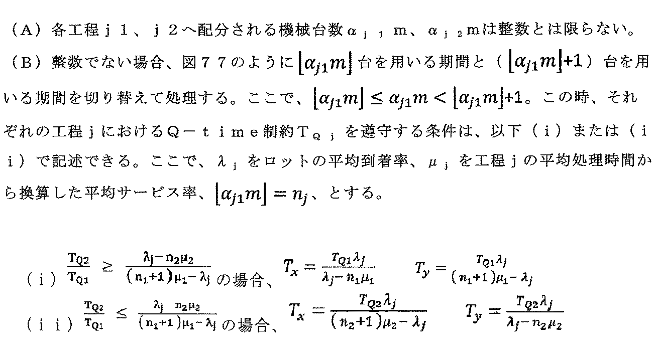
複数Q-time制約区間への生産能力の最適な配分方法を、以下(A)、(B)の前提をおいて、(i)、(ii)の場合分けを用いて実現する。このように、複数の工程が同一装置群を共用し、かつ、各工程での-time制約時間が異なる場合の扱いを定めた。
同一の装置で同時に処理する品種スペック数は1つに限られる。そのため、複数品種で共用される装置では、段取り替えをして異なる品種を異なる時期に処理する形態で共用する。
図77に示した2品種の例を、3品種以上の一般形に拡張する。
3回以上の繰返し処理がある場合として、処理工程iにおけるQ-time制約をTQi(i=1,2,・・・,n)、また、処理工程iが共用装置を使用する期間を、TXiとする。
期間TXiに共用装置を使用する工程i、期間TXiに共用装置を使用しないjのQ-time制約TQjを全て守りつつ、段取り周期を最大化することで段取り最小化を実現する。
各iの目標生産率平均をλ、期間TXiにおいて配分される装置台数を(mi+1)、単位装置当たりの処理能力をμi、Txi期間以外で溜まる仕掛理数量をLiとする。対象装置群における総装置台数mと各iに割り当てられる基本装置台数mi、共用装置台数msとの関係は、
図77に示した2品種の例を、3品種以上の一般形に拡張する。
3回以上の繰返し処理がある場合として、処理工程iにおけるQ-time制約をTQi(i=1,2,・・・,n)、また、処理工程iが共用装置を使用する期間を、TXiとする。
期間TXiに共用装置を使用する工程i、期間TXiに共用装置を使用しないjのQ-time制約TQjを全て守りつつ、段取り周期を最大化することで段取り最小化を実現する。
各iの目標生産率平均をλ、期間TXiにおいて配分される装置台数を(mi+1)、単位装置当たりの処理能力をμi、Txi期間以外で溜まる仕掛理数量をLiとする。対象装置群における総装置台数mと各iに割り当てられる基本装置台数mi、共用装置台数msとの関係は、



また、各工程iが仕掛品発生の期間内に発生した仕掛品の最大待ち時間は、Q-time制約で制限される最大待ち時間を超過できない。従って、全てのiについて、
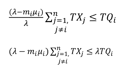


特に、最も厳しいQ-time制約の付された工程kにおいて、





第7実施形態では、さらに、図72に示す最適指標生成装置61(第6実施形態)における生産スパイクとリスクの算定に基づいて、適切な在庫の配置箇所と数量を定めて生産期間を短縮する方法を示す。まず、生産期間の短縮の重要性について説明する。生産工程において、高額で台数が限られて生産工程全体の生産率を決定づける資源的ボトルネック(例えば、半導体製造におけるフォトリソグラフィー装置等)の生産能力を高く維持することが重要である。しかし、実態として、資源的ボトルネックや非資源的ボトルネックにおける装置の保全や故障などに起因する装置の停止によって装置群の生産能力の低下が発生し、生産物流の変動(特に、装置群の生産率がボトルネックの(目標または最大)生産率以下に陥いる低下期、および、その後の復旧期が形成する生産スパイク)を引き起こし、生産物流としてボトルネックに伝搬し、資源的ボトルネックの生産率を低下させることがある。また、資源的ボトルネックの前後などにQ-time制約区間が存在し、Q-time制約区間における生産物流制御が資源的ボトルネックの生産率に影響を与えることがある。このような装置群の生産能力の変化やQ-time制約区間の生産物流制御による影響を吸収するために、半導体製造工程では、一般的に、工程間に多量の中間在庫(実態としては工場の中のストッカや搬送経路上のバッファに格納される)を配備している。この中間在庫の影響で、半導体製造における生産期間の40~65%程度を工程間の処理待ち時間が占めており、長大な生産期間(一般的に1.5~2.5ヵ月)の原因となり、時間競争力が向上せず製品の死蔵化の一因にもなっている。
第7実施形態では、生産期間の問題を解決するために、図83に示す、到着連動集中在庫型方式と図84に示す段階的変動吸収分散在庫型方式の2種類の方式を示す。資源的ボトルネック間や動的ボトルネック間やQ-time制約区間を管理単位(工程管理モジュールと呼ぶ)として、これらの方式により、最小の安全在庫量の配置と数量を定める。
I.到着連動集中在庫型方式
生産工程で起こった装置停止(予防保全時)による生産物流率のスパイクを、Q-time制約などの製造条件としての時間的制約が付されていない工程区間にまとめて中間在庫を持たせて取り除き、後続の資源的ボトルネック工程(リソグラフィー工程)などへ当該装置停止による物流変動を伝搬させない方式を指す。ここで、工場では、基本的に同様の考え方で「大量の在庫」を抱えていることが本質的に問題であるので、このスパイク除去のための在庫量を適正化(最小化)することが課題になる。到着連動集中在庫型方式では、変動が少なくQ-time制約などが設定されていないような生産リスクの小さい工程区間に安全在庫を置き、能力低下が発生した工程のロット退去(生産物流率)の変化に関わらず、安全在庫を配置した工程以降では生産率が一定(平準)になるように制御する。なお、この方法では、Q-time制約区間では、原則として、手続き型CKB=JAMP-wS2法で、装置停止によって発生する低下期と復旧期の生産能力(生産率)に連動して各Q-time制約のCKB法最適管理値が再計算・再設定される。各工程間に余計な在庫を配置しない場合、工程の利用率が100%を超えない限りはロットの到着に追従するように連動して稼動する。図83のように、装置集中停止時間tdによって発生するスパイクを取り除くための中間在庫LrはLr=λ0trとなる。ここで、制約が付されていない工程区間にまとめて取り除くためtr=td。
到着連動集中在庫型方式の利点は、在庫集約により同一サービスレベルをより少ない在庫で達成することが可能になる点である。手前の複数の工程での装置停止の影響を一手に吸収する点にある。到着連動集中在庫型方式に想定される欠点は、バッチ処理工程のように一定の在庫を要する工程の中間在庫を活用しないことや、全ての区間にQ-time制約が付された場合、対応できない点が挙げられる。
生産工程で起こった装置停止(予防保全時)による生産物流率のスパイクを、Q-time制約などの製造条件としての時間的制約が付されていない工程区間にまとめて中間在庫を持たせて取り除き、後続の資源的ボトルネック工程(リソグラフィー工程)などへ当該装置停止による物流変動を伝搬させない方式を指す。ここで、工場では、基本的に同様の考え方で「大量の在庫」を抱えていることが本質的に問題であるので、このスパイク除去のための在庫量を適正化(最小化)することが課題になる。到着連動集中在庫型方式では、変動が少なくQ-time制約などが設定されていないような生産リスクの小さい工程区間に安全在庫を置き、能力低下が発生した工程のロット退去(生産物流率)の変化に関わらず、安全在庫を配置した工程以降では生産率が一定(平準)になるように制御する。なお、この方法では、Q-time制約区間では、原則として、手続き型CKB=JAMP-wS2法で、装置停止によって発生する低下期と復旧期の生産能力(生産率)に連動して各Q-time制約のCKB法最適管理値が再計算・再設定される。各工程間に余計な在庫を配置しない場合、工程の利用率が100%を超えない限りはロットの到着に追従するように連動して稼動する。図83のように、装置集中停止時間tdによって発生するスパイクを取り除くための中間在庫LrはLr=λ0trとなる。ここで、制約が付されていない工程区間にまとめて取り除くためtr=td。
到着連動集中在庫型方式の利点は、在庫集約により同一サービスレベルをより少ない在庫で達成することが可能になる点である。手前の複数の工程での装置停止の影響を一手に吸収する点にある。到着連動集中在庫型方式に想定される欠点は、バッチ処理工程のように一定の在庫を要する工程の中間在庫を活用しないことや、全ての区間にQ-time制約が付された場合、対応できない点が挙げられる。
(事例)図58に示した非特許文献1の生産工程モデル:
フォトリソグラフィー~「DRY1-WET(1)-Fur(1)-DRY2-WET(2)-N2-Fur(2)」~フォトリソグラフィーの区間で、Fur(1)の予防保全が起こる場合を例に説明を加える。
Fur(1)は、定常時は、利用率80%程度である。
ここで、Fur(1)において、Fur(1)の利用率100%を超えるような装置停止が起こったとする。これは、前述の通り、同時に一定台数以上が保全や故障などのため停止する場合である(このような低下が起こらないように保全時期を分散化するが、万一起こった場合について)。
予め、このような低下期に陥ることが分かっている場合には、第3実施形態で示したように、所定の時点で予め、Fur(1)に関わるQ-time制約区間:DRY1-WET(1)-Fur(1)の最適仕掛管理値を再計算して置き換えることで、Q-time制約の超過を防ぐと共に目標生産率の達成を目指す(第3実施形態)。
ここで、Q-time制約区間の最終工程:Fur(1)のロット退出率は、処理開始と同様の形となり、定常期、低下期、復旧期と大きく変化する。この生産物流率の生産スパイクを、次の資源的ボトルネック装置群(フォトリソグラフィー工程)に伝搬させないよう、速やかに後続の非Q-time制約区間:Fur(1)-Dry(2)で除去する。そのためにDry(2)の仕掛りロット(中間在庫)を最大の生産スパイクを吸収する程度溜めておく。
このような中間在庫は、常にためておく必要はない。仮に予防保全など予め実施時期が決められた場合には、その時期に合わせて溜めてゆけばよい(例えば、Dry(2)では、偶発故障が起こるため、その際に処理しきれなかった分が溜まる機会もある。)。
フォトリソグラフィー~「DRY1-WET(1)-Fur(1)-DRY2-WET(2)-N2-Fur(2)」~フォトリソグラフィーの区間で、Fur(1)の予防保全が起こる場合を例に説明を加える。
Fur(1)は、定常時は、利用率80%程度である。
ここで、Fur(1)において、Fur(1)の利用率100%を超えるような装置停止が起こったとする。これは、前述の通り、同時に一定台数以上が保全や故障などのため停止する場合である(このような低下が起こらないように保全時期を分散化するが、万一起こった場合について)。
予め、このような低下期に陥ることが分かっている場合には、第3実施形態で示したように、所定の時点で予め、Fur(1)に関わるQ-time制約区間:DRY1-WET(1)-Fur(1)の最適仕掛管理値を再計算して置き換えることで、Q-time制約の超過を防ぐと共に目標生産率の達成を目指す(第3実施形態)。
ここで、Q-time制約区間の最終工程:Fur(1)のロット退出率は、処理開始と同様の形となり、定常期、低下期、復旧期と大きく変化する。この生産物流率の生産スパイクを、次の資源的ボトルネック装置群(フォトリソグラフィー工程)に伝搬させないよう、速やかに後続の非Q-time制約区間:Fur(1)-Dry(2)で除去する。そのためにDry(2)の仕掛りロット(中間在庫)を最大の生産スパイクを吸収する程度溜めておく。
このような中間在庫は、常にためておく必要はない。仮に予防保全など予め実施時期が決められた場合には、その時期に合わせて溜めてゆけばよい(例えば、Dry(2)では、偶発故障が起こるため、その際に処理しきれなかった分が溜まる機会もある。)。
半導体加工寸法の微細化(高度化)に伴い、生産工程上のQ-time制約区間は増加の一途にあるため、到着連動集中在庫型方式のようにQ-time制約区間では生産物流率のスパイクに対応しないと限定すると、このスパイク低減に限界が出る可能性がある。また、中間在庫を持たせる工程は、バッチ型などある一定以上の在庫を当初から必要とする工程や、また装置が偶発故障しづらい装置群が適しており、それが必ずしもQ-time制約区間以外であるとは限らない。先の工程モデルの例でいえば、WETやFURは、バッチ型でかつ偶発故障がほとんどない装置の典型例である。そこで、以下の段階的変動吸収分散在庫型方式の利用を考える。
II.段階的変動吸収分散在庫型方式
到着連動集中在庫型方式との違いは、Q-time制約の有無に関わらずバッチ処理工程など一定の在庫を要する工程区間の在庫を活用して、順次可能な限り生産スパイクを低減していく点である。また、資源的ボトルネック工程の目標生産率との乖離を減らすために、バッチ工程でのロードサイズを適切に変更する。
図84のような装置集中停止時間tdによって発生するスパイクを取り除くための中間在庫LriはLri=λ0triとなる。
ここで、制約が付されてるため、制約時間Tqi<tr1のときtr1=Tq1。
そして、後継制約区間の時間長tr(i+1)は

となる。
段階的変動吸収分散在庫型方式の利点は、プロセスの高度化の影響で増加の一途にあるQ-time制約が点在する生産工程でも、各工程の中間在庫を活用して可能な限り生産スパイクを段階的に低減し、資源的ボトルネック工程へのスパイクの伝搬を早い段階で防ぐ可能性を高める点にある。また、バッチ工程でのローディングを生産工程全体に合致させるよう適正化する。段階的変動吸収分散在庫型方式の想定される欠点は、バッチ工程でローディングサイズを小さくすることを許容すると、同一期間長におけるローディング回数を増やすことになり、熱処理炉(Fur)などの装置群では予防保全周期が短くなることがあり、注意を払う必要がある。
到着連動集中在庫型方式との違いは、Q-time制約の有無に関わらずバッチ処理工程など一定の在庫を要する工程区間の在庫を活用して、順次可能な限り生産スパイクを低減していく点である。また、資源的ボトルネック工程の目標生産率との乖離を減らすために、バッチ工程でのロードサイズを適切に変更する。
図84のような装置集中停止時間tdによって発生するスパイクを取り除くための中間在庫LriはLri=λ0triとなる。
ここで、制約が付されてるため、制約時間Tqi<tr1のときtr1=Tq1。
そして、後継制約区間の時間長tr(i+1)は
となる。
段階的変動吸収分散在庫型方式の利点は、プロセスの高度化の影響で増加の一途にあるQ-time制約が点在する生産工程でも、各工程の中間在庫を活用して可能な限り生産スパイクを段階的に低減し、資源的ボトルネック工程へのスパイクの伝搬を早い段階で防ぐ可能性を高める点にある。また、バッチ工程でのローディングを生産工程全体に合致させるよう適正化する。段階的変動吸収分散在庫型方式の想定される欠点は、バッチ工程でローディングサイズを小さくすることを許容すると、同一期間長におけるローディング回数を増やすことになり、熱処理炉(Fur)などの装置群では予防保全周期が短くなることがあり、注意を払う必要がある。
事例を用いて、段階的変動吸収分散在庫型方式の動作を説明する。
先の図58の生産工程モデルのDRY1とDRY2は、不安定なプラズマ系プロセスを採用している装置のため偶発故障が発生する。なお、DRY1、DRY2共にQ-time制約区間の先頭工程であるためQ-time制約の遵守には問題ない。故障により処理中止などを強いられたロット(ウェハ群)は没となる。
一般的な運用条件としてFurの稼働率が80%(通常可動、停止無し)となるリソグラフィー工程の平均生産率である場合に、DRY1で低下期が発生するのは、同時に10台以上ダウンした場合である。(全部でDRY1は装置16台、DRY2も別の装置16台があるモデル)
前の工程j(例えばDRY1)で故障による装置停止の影響で低下期(生産率μ_(d,j)<当初目標生産率(平均)λ)になる。低下期が始まっても、次の工程(WET(1))以降ではQ-time制約を守りつつ、中間在庫(仕掛りロット)が一定以下(特段の定めなえればゼロ)になるまで同じ生産率(当初目標生産率(平均)λ)で処理を続ける。
中間在庫が一定以下(特段の定めなえればゼロ)になった後は、到着ロットに合わせて処理を開始する(低下期の終了時点=復旧期の開始時点まで)。
もし、復旧期のDRY1の生産率μ_(r,j)(=WET(1)へのロット到着率)がWET(1)の平均処理能力より勝っていた場合、WET(1)でのロット仕掛数が増えていく。その仕掛数がQ-time制約を遵守するための最大ロット数に達したら、再度CKB法の上限管理が機能し始める(図84の変化点)。
この場合、CKB法最適値計算に使用する平均到着率は前の工程(Dry1)の復旧期の生産率μ_(r,j)(>λ)となる。低下期の期間tdと当初目標生産率(平均)λがわかっているので、復旧期の長さYは見積もることができる。Y=td(λ―μ_(d,j))/μ_(r,j)。偶発故障時でも復旧終了時点で見積もることができる。
こうして、装置停止の後続工程でQ-time制約区間でもQ-time制約を守りつつ、段階的に生産物流のスパイクを減らしていく。
先の図58の生産工程モデルのDRY1とDRY2は、不安定なプラズマ系プロセスを採用している装置のため偶発故障が発生する。なお、DRY1、DRY2共にQ-time制約区間の先頭工程であるためQ-time制約の遵守には問題ない。故障により処理中止などを強いられたロット(ウェハ群)は没となる。
一般的な運用条件としてFurの稼働率が80%(通常可動、停止無し)となるリソグラフィー工程の平均生産率である場合に、DRY1で低下期が発生するのは、同時に10台以上ダウンした場合である。(全部でDRY1は装置16台、DRY2も別の装置16台があるモデル)
前の工程j(例えばDRY1)で故障による装置停止の影響で低下期(生産率μ_(d,j)<当初目標生産率(平均)λ)になる。低下期が始まっても、次の工程(WET(1))以降ではQ-time制約を守りつつ、中間在庫(仕掛りロット)が一定以下(特段の定めなえればゼロ)になるまで同じ生産率(当初目標生産率(平均)λ)で処理を続ける。
中間在庫が一定以下(特段の定めなえればゼロ)になった後は、到着ロットに合わせて処理を開始する(低下期の終了時点=復旧期の開始時点まで)。
もし、復旧期のDRY1の生産率μ_(r,j)(=WET(1)へのロット到着率)がWET(1)の平均処理能力より勝っていた場合、WET(1)でのロット仕掛数が増えていく。その仕掛数がQ-time制約を遵守するための最大ロット数に達したら、再度CKB法の上限管理が機能し始める(図84の変化点)。
この場合、CKB法最適値計算に使用する平均到着率は前の工程(Dry1)の復旧期の生産率μ_(r,j)(>λ)となる。低下期の期間tdと当初目標生産率(平均)λがわかっているので、復旧期の長さYは見積もることができる。Y=td(λ―μ_(d,j))/μ_(r,j)。偶発故障時でも復旧終了時点で見積もることができる。
こうして、装置停止の後続工程でQ-time制約区間でもQ-time制約を守りつつ、段階的に生産物流のスパイクを減らしていく。
第7実施形態では、第4実施形態と第6実施形態の変形例として、管理対象とする生産工程の全ての装置群についてJAMP-wS法により算定される保全や段取り時期により発生する静的生産スパイクに動的な故障などを合わせた動的生産スパイクを複数の生産工程について重ね合わせた複合スパイクを分析し、対象とする生産工程における生産スパイクを最小の安全在庫で吸収して、生産工程全体の生産率を決定づける資源的ボトルネックにおける生産率低下を防ぎながら、在庫の削減と生産期間の短縮化を図る方法を示した。
<第8実施形態>
図85を参照して、本発明の第8実施形態に係る最適指標生成方法について説明する。なお、本実施形態は、第1実施形態に係る最適指標生成装置を構成する各部の動作について、下記のフローチャートで示すプログラムをプロセッサに実行させたことを特徴としている。各ステップはソフトウエアモジュールの動作内容を示しており、詳細な動作内容については第1実施形態に記載しているので、その説明を省略する。
最適指標生成装置に電源が投入されると、CPUは、補助記憶部から読み込んだOSをRAM上にブートして実行する。そして、CPUは、このOS上で補助記憶部からRAM上に読み出したアプリケーションソフトウエアの一例として下記の最適指標生成アプリケーションプログラムを実行する。
図85を参照して、本発明の第8実施形態に係る最適指標生成方法について説明する。なお、本実施形態は、第1実施形態に係る最適指標生成装置を構成する各部の動作について、下記のフローチャートで示すプログラムをプロセッサに実行させたことを特徴としている。各ステップはソフトウエアモジュールの動作内容を示しており、詳細な動作内容については第1実施形態に記載しているので、その説明を省略する。
最適指標生成装置に電源が投入されると、CPUは、補助記憶部から読み込んだOSをRAM上にブートして実行する。そして、CPUは、このOS上で補助記憶部からRAM上に読み出したアプリケーションソフトウエアの一例として下記の最適指標生成アプリケーションプログラムを実行する。
なお、本実施形態にあっては、多品種の製品を生産するため複数の装置を制御する生産管理システムに対して、前記複数の装置と製品に関する指標情報を供給することを特徴とする。
まず、ステップS301では、複数の装置と製品に関する情報を生産管理システムを介して入力する。次いで、ステップS303では、製品の到着に関連するバッチ組待ち時間とQ-time制約の上限値との大小関係が切り替わる到着率の境界値を算定し、適切なロードルールを判定する。
次いで、ステップS303では、入力された情報から複数の装置による加工工程間の滞在時間の制限値を示すQ-time構造を分析し、内部記憶部14aに記憶する。
次いで、ステップS304では、入力された情報およびQ-time構造に基づいて、品種別の最適なカンバン枚数およびバッファサイズを計算する。
次いで、ステップS305では、計算された情報を指標情報として出力する。次いで、ステップS306では、算出された最適な指標情報とロードルールとを生産管理システムに供給する。
まず、ステップS301では、複数の装置と製品に関する情報を生産管理システムを介して入力する。次いで、ステップS303では、製品の到着に関連するバッチ組待ち時間とQ-time制約の上限値との大小関係が切り替わる到着率の境界値を算定し、適切なロードルールを判定する。
次いで、ステップS303では、入力された情報から複数の装置による加工工程間の滞在時間の制限値を示すQ-time構造を分析し、内部記憶部14aに記憶する。
次いで、ステップS304では、入力された情報およびQ-time構造に基づいて、品種別の最適なカンバン枚数およびバッファサイズを計算する。
次いで、ステップS305では、計算された情報を指標情報として出力する。次いで、ステップS306では、算出された最適な指標情報とロードルールとを生産管理システムに供給する。
また、図86に示すフローチャートを参照すると、ステップS311では、ステップS304により算出された最適な指標情報に対して、感度解析を予め行っておき、内部記憶部に記憶する。ステップS312では、各種入力情報の変動に対応した最適な指標情報を即時に生産管理システムに供給する。
また、図87に示すフローチャートを参照すると、ステップS315では、後続工程区間または先行工程区間のスループットの変化に連動してカンバン枚数やバッファサイズを変更する。
また、図88に示すフローチャートを参照すると、ステップS317では、加工工程間で待つことが可能な最大ロット数を超えないように、複数の装置による加工工程間に設けられたバッファのサイズを制限することにより、先行工程の製品の出力を制御する。
また、図87に示すフローチャートを参照すると、ステップS315では、後続工程区間または先行工程区間のスループットの変化に連動してカンバン枚数やバッファサイズを変更する。
また、図88に示すフローチャートを参照すると、ステップS317では、加工工程間で待つことが可能な最大ロット数を超えないように、複数の装置による加工工程間に設けられたバッファのサイズを制限することにより、先行工程の製品の出力を制御する。
また、図89に示すフローチャートを参照すると、ステップS318では、Q-time制約区間内のボトルネック箇所のトラフィック強度が1を超えないように制御する。ステップS319では、トラフィック強度が1より大きい場合には、λはトラフィック強度(ρ)が1の時の投入率とする。
また、図90に示すフローチャートを参照すると、ステップS320では、Q-time制約区間内に滞在するロットの数を製品品種および処理条件別のカンバン枚数によって制限し、各ロットの処理開始時期を空きカンバンによって制御する。
また、図90に示すフローチャートを参照すると、ステップS320では、Q-time制約区間内に滞在するロットの数を製品品種および処理条件別のカンバン枚数によって制限し、各ロットの処理開始時期を空きカンバンによって制御する。
次に、図91を参照して、本発明の第8実施形態に係る最適指標生成方法の変形例として、下記のフローチャートで示すプログラムをサーバに設けられたプロセッサに実行させたこととして説明する。
なお、本変形例であっては、多品種の製品を生産するため複数の装置を制御する生産管理システムに対して、通信回線を介して複数の装置と製品に関する指標情報を送信するサーバが実行することを特徴とする。また、サーバには通信制御部が設けられており、通信制御部が生産管理システムと通信回線を介して情報を通信することとする。
なお、本変形例であっては、多品種の製品を生産するため複数の装置を制御する生産管理システムに対して、通信回線を介して複数の装置と製品に関する指標情報を送信するサーバが実行することを特徴とする。また、サーバには通信制御部が設けられており、通信制御部が生産管理システムと通信回線を介して情報を通信することとする。
まず、ステップS321では、複数の装置と製品に関する情報を生産管理システムを介して受信する。次いで、ステップS322では、受信された情報から複数の装置による加工工程間の滞在時間の制限値を示すQ-time構造を分析し、内部記憶部に記憶する。
次いで、ステップS323では、計算された情報を指標情報として出力する。
次いで、ステップS324では、製品の到着に関連するバッチ組待ち時間とQ-time制約の上限値との大小関係が切り替わる到着率の境界値を算定し、適切なロードルールを判定する。
次いで、ステップS325では、受信された情報およびQ-time構造に基づいて、品種別の最適なカンバン枚数およびバッファサイズを計算する。次いで、ステップS326では、算出された最適な指標情報とロードルールとを生産管理システムに送信する。
次いで、ステップS323では、計算された情報を指標情報として出力する。
次いで、ステップS324では、製品の到着に関連するバッチ組待ち時間とQ-time制約の上限値との大小関係が切り替わる到着率の境界値を算定し、適切なロードルールを判定する。
次いで、ステップS325では、受信された情報およびQ-time構造に基づいて、品種別の最適なカンバン枚数およびバッファサイズを計算する。次いで、ステップS326では、算出された最適な指標情報とロードルールとを生産管理システムに送信する。
以上のようにQ-time制約を守りつつ他の性能指標も悪化させない生産スケジューリング手法として、計算スピード、精度、実用性などの定性的評価も高いCKB法の構築と性能評価と通して目的を達成することができた。
<第9実施形態>
図92を参照して、本発明の第9実施形態に係る最適指標生成方法について説明する。なお、本実施形態は、第4実施形態に係る最適指標生成装置を構成する各部の動作について、下記のフローチャートで示すプログラムをプロセッサに実行させたことを特徴としている。各ステップはソフトウエアモジュールの動作内容を示しており、詳細な動作内容については第1実施形態に記載しているので、その説明を省略する。
最適指標生成装置に電源が投入されると、CPUは、補助記憶部から読み込んだOSをRAM上にブートして実行する。そして、CPUは、このOS上で補助記憶部からRAM上に読み出したアプリケーションソフトウエアの一例として下記の最適指標生成アプリケーションプログラムを実行する。
図92を参照して、本発明の第9実施形態に係る最適指標生成方法について説明する。なお、本実施形態は、第4実施形態に係る最適指標生成装置を構成する各部の動作について、下記のフローチャートで示すプログラムをプロセッサに実行させたことを特徴としている。各ステップはソフトウエアモジュールの動作内容を示しており、詳細な動作内容については第1実施形態に記載しているので、その説明を省略する。
最適指標生成装置に電源が投入されると、CPUは、補助記憶部から読み込んだOSをRAM上にブートして実行する。そして、CPUは、このOS上で補助記憶部からRAM上に読み出したアプリケーションソフトウエアの一例として下記の最適指標生成アプリケーションプログラムを実行する。
なお、本実施形態にあっては、多品種の製品を生産するための生産実行システムに設けられた複数の装置を制御する生産管理システムに対して、複数の装置に関する指標情報を供給することを特徴とする。
次いで、ステップS331では、生産実行システムに含まれる複数の装置と製品に関する情報を生産管理システムを介して入力する。
次いで、ステップS332では、入力された情報から複数の装置による加工工程の中のボトルネック箇所および最大流量を解析する。
次いで、ステップS333では、入力された情報から1つ以上のQ-time制約が存在しているQ-time制約区間の構造を分析し、内部記憶部に記憶する。
次いで、ステップS334では、S333で内部記憶部に記憶した情報を用いて、全てのQ-time制約区間について最適指標計算を完了したか否かを判断する。最適指標計算を完了した場合には、ステップS339に進む。最適指標計算を完了していない場合には、ステップS335に進む。
次いで、ステップS331では、生産実行システムに含まれる複数の装置と製品に関する情報を生産管理システムを介して入力する。
次いで、ステップS332では、入力された情報から複数の装置による加工工程の中のボトルネック箇所および最大流量を解析する。
次いで、ステップS333では、入力された情報から1つ以上のQ-time制約が存在しているQ-time制約区間の構造を分析し、内部記憶部に記憶する。
次いで、ステップS334では、S333で内部記憶部に記憶した情報を用いて、全てのQ-time制約区間について最適指標計算を完了したか否かを判断する。最適指標計算を完了した場合には、ステップS339に進む。最適指標計算を完了していない場合には、ステップS335に進む。
次いで、ステップS335では、製品の到着に関連するバッチ組待ち時間とQ-time制約の上限値との大小関係が切り替わる到着率の境界値を算定し、適切なロードルールを判定する。
次いで、ステップS336では、複数の装置を常用能力を有する常用装置と代替能力を有する代替装置とに区分する。
次いで、ステップS337では、Q-time制約区間の中のボトルネック箇所および最大流量を解析する。
次いで、ステップS338では、ボトルネック箇所、最大流量および前記Q-time構造に基づいて、品種別の最適なカンバン枚数およびバッファサイズと、常用装置と代替装置とに関する生産負荷と予防保全開始時期を計算して指標情報として内部記憶部に記憶し、ステップS334に進む。
次いで、ステップS339では、S338で内部記憶部に記憶された最適な指標情報を生産管理システムやエンジニアリング業務システムに供給するとともに、時間指標算出ステップにより算出された最適な指標情報を生産管理システムに供給し、処理を終了する。
次いで、ステップS336では、複数の装置を常用能力を有する常用装置と代替能力を有する代替装置とに区分する。
次いで、ステップS337では、Q-time制約区間の中のボトルネック箇所および最大流量を解析する。
次いで、ステップS338では、ボトルネック箇所、最大流量および前記Q-time構造に基づいて、品種別の最適なカンバン枚数およびバッファサイズと、常用装置と代替装置とに関する生産負荷と予防保全開始時期を計算して指標情報として内部記憶部に記憶し、ステップS334に進む。
次いで、ステップS339では、S338で内部記憶部に記憶された最適な指標情報を生産管理システムやエンジニアリング業務システムに供給するとともに、時間指標算出ステップにより算出された最適な指標情報を生産管理システムに供給し、処理を終了する。
また、図93に示すフローチャートを参照すると、ステップS341では、生産実行システムに含まれる製造フロー全体に点在するすべてのQ-time制約を同時に管理する。
また、図94に示すフローチャートを参照すると、ステップS343では、生産実行システムに含まれる製造フロー全体における生産流量や工程能力の変動に対応してQ-time制約を同時に管理するために、製造フローにおけるボトルネック箇所と各工程の最大流量を解析する。
また、図94に示すフローチャートを参照すると、ステップS343では、生産実行システムに含まれる製造フロー全体における生産流量や工程能力の変動に対応してQ-time制約を同時に管理するために、製造フローにおけるボトルネック箇所と各工程の最大流量を解析する。
次に、図95を参照して、本発明の第9実施形態に係る最適指標生成方法の変形例として、下記のフローチャートで示すプログラムをサーバに設けられたプロセッサに実行させたこととして説明する。
なお、本変形例であっては、多品種の製品を生産するための生産実行システムに設けられた複数の装置を制御する生産管理システムに対して、通信回線介して前記複数の装置に関する指標情報を送信するサーバが実行することを特徴とする。また、サーバには通信制御部が設けられており、通信制御部が生産管理システムと通信回線を介して情報を通信することとする。
なお、本変形例であっては、多品種の製品を生産するための生産実行システムに設けられた複数の装置を制御する生産管理システムに対して、通信回線介して前記複数の装置に関する指標情報を送信するサーバが実行することを特徴とする。また、サーバには通信制御部が設けられており、通信制御部が生産管理システムと通信回線を介して情報を通信することとする。
次いで、ステップS351では、生産実行システムに含まれる複数の装置と製品に関する情報を生産管理システムを介して受信する。
次いで、ステップS352では、受信された情報から複数の装置による加工工程の中のボトルネック箇所および最大流量を解析する。
次いで、ステップS353では、受信された情報から1つ以上のQ-time制約が存在しているQ-time制約区間の構造を分析し、内部記憶部に記憶する。
次いで、ステップS354では、S353で内部記憶部に記憶した情報を用いて、全てのQ-time制約区間について最適指標計算を完了したか否かを判断する。最適指標計算を完了した場合には、ステップS359に進む。最適指標計算を完了していない場合には、ステップS355に進む。
次いで、ステップS352では、受信された情報から複数の装置による加工工程の中のボトルネック箇所および最大流量を解析する。
次いで、ステップS353では、受信された情報から1つ以上のQ-time制約が存在しているQ-time制約区間の構造を分析し、内部記憶部に記憶する。
次いで、ステップS354では、S353で内部記憶部に記憶した情報を用いて、全てのQ-time制約区間について最適指標計算を完了したか否かを判断する。最適指標計算を完了した場合には、ステップS359に進む。最適指標計算を完了していない場合には、ステップS355に進む。
次いで、ステップS355では、製品の到着に関連するバッチ組待ち時間とQ-time制約の上限値との大小関係が切り替わる到着率の境界値を算定し、適切なロードルールを判定する。
次いで、ステップS356では、複数の装置を常用能力を有する常用装置と代替能力を有する代替装置とに区分する。
次いで、ステップS357では、Q-time制約区間の中のボトルネック箇所および最大流量を解析する。
次いで、ステップS358では、ボトルネック箇所、最大流量および前記Q-time構造に基づいて、品種別の最適なカンバン枚数およびバッファサイズを計算して指標情報として内部記憶部に記憶し、ステップS354に進む。
次いで、ステップS359では、S358で内部記憶部に記憶された最適な指標情報を生産管理システムやエンジニアリング業務システムに送信するとともに、時間指標算出ステップにより算出された最適な指標情報を生産管理システムに送信し、処理を終了する。
次いで、ステップS356では、複数の装置を常用能力を有する常用装置と代替能力を有する代替装置とに区分する。
次いで、ステップS357では、Q-time制約区間の中のボトルネック箇所および最大流量を解析する。
次いで、ステップS358では、ボトルネック箇所、最大流量および前記Q-time構造に基づいて、品種別の最適なカンバン枚数およびバッファサイズを計算して指標情報として内部記憶部に記憶し、ステップS354に進む。
次いで、ステップS359では、S358で内部記憶部に記憶された最適な指標情報を生産管理システムやエンジニアリング業務システムに送信するとともに、時間指標算出ステップにより算出された最適な指標情報を生産管理システムに送信し、処理を終了する。
これにより、従来法では達成されていなかったQ-time制約割れが起こりやすい状況に対しても、Q-time制約を確実に遵守し、良品スループット向上とコスト低減および環境負荷低減を達成することが可能な最適オペレーション管理条件を提供することができる。
また、Q-time制約割れの主要な原因である、多品種生産の扱い、装置の予防保全、複数のQ-time制約の相互干渉に対しても、解析方法と適正な管理手法を与えることで、Q-time制約遵守しつつ良品スループットの向上とコスト低減・環境負荷低減を同時に達成することができる。
また、Q-time制約割れの主要な原因である、多品種生産の扱い、装置の予防保全、複数のQ-time制約の相互干渉に対しても、解析方法と適正な管理手法を与えることで、Q-time制約遵守しつつ良品スループットの向上とコスト低減・環境負荷低減を同時に達成することができる。
<第10実施形態>
図96を参照して、本発明の第10実施形態に係る最適指標生成方法について説明する。なお、本実施形態は、第2実施形態に係る最適指標生成装置を構成する各部の動作について、下記のフローチャートで示すプログラムをプロセッサに実行させたことを特徴としている。各ステップはソフトウエアモジュールの動作内容を示しており、詳細な動作内容については第1実施形態に記載しているので、その説明を省略する。
最適指標生成装置に電源が投入されると、CPUは、補助記憶部から読み込んだOSをRAM上にブートして実行する。そして、CPUは、このOS上で補助記憶部からRAM上に読み出したアプリケーションソフトウエアの一例として下記の最適指標生成アプリケーションプログラムを実行することを特徴とする。
図96を参照して、本発明の第10実施形態に係る最適指標生成方法について説明する。なお、本実施形態は、第2実施形態に係る最適指標生成装置を構成する各部の動作について、下記のフローチャートで示すプログラムをプロセッサに実行させたことを特徴としている。各ステップはソフトウエアモジュールの動作内容を示しており、詳細な動作内容については第1実施形態に記載しているので、その説明を省略する。
最適指標生成装置に電源が投入されると、CPUは、補助記憶部から読み込んだOSをRAM上にブートして実行する。そして、CPUは、このOS上で補助記憶部からRAM上に読み出したアプリケーションソフトウエアの一例として下記の最適指標生成アプリケーションプログラムを実行することを特徴とする。
なお、本実施形態にあっては、多品種の製品を生産するための複数の装置を制御する生産管理システムに対して、前記複数の装置に関する指標情報を供給することを特徴とする。
まず、ステップS361では、複数の装置に関する情報を生産管理システムを介して入力する。次いで、ステップS362では、複数の装置を常用能力を有する常用装置と代替能力を有する代替装置とに区分する。次いで、ステップS363では、算定された装置区分と入力された情報から複数の常用装置と代替装置の稼働回数(生産負荷)と稼働時期を算出する。
次いで、ステップS364では、計算出結果から常用装置と代替装置とに関する予防保全開始・終了時期を算出する。次いで、ステップS365では、算出された最適な開始終了時期情報を生産管理システムやエンジニアリング業務システムに供給する。
まず、ステップS361では、複数の装置に関する情報を生産管理システムを介して入力する。次いで、ステップS362では、複数の装置を常用能力を有する常用装置と代替能力を有する代替装置とに区分する。次いで、ステップS363では、算定された装置区分と入力された情報から複数の常用装置と代替装置の稼働回数(生産負荷)と稼働時期を算出する。
次いで、ステップS364では、計算出結果から常用装置と代替装置とに関する予防保全開始・終了時期を算出する。次いで、ステップS365では、算出された最適な開始終了時期情報を生産管理システムやエンジニアリング業務システムに供給する。
また、図97に示すフローチャートを参照すると、ステップS371では、最適理論値計算ステップにより算出された最適な開始終了時期情報に対して、感度解析を予め行っておき、内部記憶部に記憶する。次いで、ステップS372では、各種入力情報の変動に対応した最適な指標情報を即時に前記生産管理システムに供給する。
次に、図98を参照して、本発明の第10実施形態に係る最適指標生成方法の変形例として、下記のフローチャートで示すプログラムをサーバに設けられたプロセッサに実行させたこととして説明する。
なお、本変形例であっては、多品種の製品を生産するための複数の装置を制御する生産管理システムに対して、通信回線を介して複数の装置に関する指標情報を送信するサーバが実行することを特徴とする。また、サーバには通信制御部が設けられており、通信制御部が生産管理システムと通信回線を介して情報を通信することとする。
まず、ステップS381では、複数の装置に関する情報を生産管理システムを介して受信する。次いで、ステップS382では、複数の装置を常用能力を有する常用装置と代替能力を有する代替装置とに区分する。次いで、ステップS383では、算定された装置区分と受信された情報から複数の常用装置と代替装置の稼働回数(生産負荷)と稼働時期を算出する。
次いで、ステップS384では、計算出結果から常用装置と代替装置とに関する予防保全開始・終了時期を算出する。次いで、ステップS385では、算出された最適な開始終了時期情報を生産管理システムやエンジニアリング業務システムに送信する。
なお、本変形例であっては、多品種の製品を生産するための複数の装置を制御する生産管理システムに対して、通信回線を介して複数の装置に関する指標情報を送信するサーバが実行することを特徴とする。また、サーバには通信制御部が設けられており、通信制御部が生産管理システムと通信回線を介して情報を通信することとする。
まず、ステップS381では、複数の装置に関する情報を生産管理システムを介して受信する。次いで、ステップS382では、複数の装置を常用能力を有する常用装置と代替能力を有する代替装置とに区分する。次いで、ステップS383では、算定された装置区分と受信された情報から複数の常用装置と代替装置の稼働回数(生産負荷)と稼働時期を算出する。
次いで、ステップS384では、計算出結果から常用装置と代替装置とに関する予防保全開始・終了時期を算出する。次いで、ステップS385では、算出された最適な開始終了時期情報を生産管理システムやエンジニアリング業務システムに送信する。
<第11実施形態>
図99を参照して、本発明の第11実施形態に係る最適指標生成方法について説明する。なお、本実施形態は、第3実施形態に係る最適指標生成装置を構成する各部の動作について、下記のフローチャートで示すプログラムをプロセッサに実行させたことを特徴としている。各ステップはソフトウエアモジュールの動作内容を示しており、詳細な動作内容については第1実施形態に記載しているので、その説明を省略する。
最適指標生成装置に電源が投入されると、CPUは、補助記憶部から読み込んだOSをRAM上にブートして実行する。そして、CPUは、このOS上で補助記憶部からRAM上に読み出したアプリケーションソフトウエアの一例として下記の最適指標生成アプリケーションプログラムを実行する。
図99を参照して、本発明の第11実施形態に係る最適指標生成方法について説明する。なお、本実施形態は、第3実施形態に係る最適指標生成装置を構成する各部の動作について、下記のフローチャートで示すプログラムをプロセッサに実行させたことを特徴としている。各ステップはソフトウエアモジュールの動作内容を示しており、詳細な動作内容については第1実施形態に記載しているので、その説明を省略する。
最適指標生成装置に電源が投入されると、CPUは、補助記憶部から読み込んだOSをRAM上にブートして実行する。そして、CPUは、このOS上で補助記憶部からRAM上に読み出したアプリケーションソフトウエアの一例として下記の最適指標生成アプリケーションプログラムを実行する。
なお、本実施形態にあっては、多品種の製品を生産するための生産実行システムに設けられた複数の装置を制御する生産管理システムに対して、前記複数の装置に関する指標情報を供給することを特徴とする。
次いで、ステップS391では、生産実行システムに含まれる複数の装置や製品に関する情報を生産管理システムを介して入力する。
次いで、ステップS392では、入力された情報から複数の装置による加工工程間の滞在時間の制限値を示すQ-time制約を分析し、内部記憶部に記憶する。
次いで、ステップS393では、生産実行システムに含まれる複数の装置に関する情報を生産管理システムから入力する。次いで、ステップS394では、複数の装置を常用能力を有する常用装置と代替能力を有する代替装置とに区分する。
次いで、ステップS391では、生産実行システムに含まれる複数の装置や製品に関する情報を生産管理システムを介して入力する。
次いで、ステップS392では、入力された情報から複数の装置による加工工程間の滞在時間の制限値を示すQ-time制約を分析し、内部記憶部に記憶する。
次いで、ステップS393では、生産実行システムに含まれる複数の装置に関する情報を生産管理システムから入力する。次いで、ステップS394では、複数の装置を常用能力を有する常用装置と代替能力を有する代替装置とに区分する。
次いで、ステップS395では、算定された装置区分と入力された情報から複数の常用装置と代替装置の稼働回数と稼働時期を算出する。次いで、ステップS396では、常用装置と代替装置とに関する予防保全開始時期を算出する。
次いで、ステップS397では、入力された情報とQ-time構造および予防保全開始時期に基づいて、品種別の最適なカンバン枚数およびバッファサイズを計算して指標情報として出力する。
次いで、ステップS398では、算出された最適な開始終了時期情報を生産管理システムやエンジニアリング業務システムに供給するとともに、算出された開始終了時期により定まる工程能力が異なる各期に対して最適な指標情報を生産管理システムに供給する。
次いで、ステップS397では、入力された情報とQ-time構造および予防保全開始時期に基づいて、品種別の最適なカンバン枚数およびバッファサイズを計算して指標情報として出力する。
次いで、ステップS398では、算出された最適な開始終了時期情報を生産管理システムやエンジニアリング業務システムに供給するとともに、算出された開始終了時期により定まる工程能力が異なる各期に対して最適な指標情報を生産管理システムに供給する。
また、図100に示すフローチャートを参照すると、ステップS401では、算出された最適な指標情報および開始終了時期に対して、感度解析を予め行っておき、内部記憶部に記憶する。
次いで、でステップS402では、各種入力情報の変動に対応した最適な指標情報および開始終了時期情報を即時に生産管理システムに供給する。
次いで、でステップS402では、各種入力情報の変動に対応した最適な指標情報および開始終了時期情報を即時に生産管理システムに供給する。
次に、図101を参照して、本発明の第11実施形態に係る最適指標生成方法の変形例として、下記のフローチャートで示すプログラムをサーバに設けられたプロセッサに実行させたこととして説明する。
なお、本変形例であっては、多品種の製品を生産するための生産実行システムに設けられた複数の装置を制御する生産管理システムに対して、通信回線を介して前記複数の装置に関する指標情報を送信するサーバが実行することを特徴とする。また、サーバには通信制御部が設けられており、通信制御部が生産管理システムと通信回線を介して情報を通信することとする。
まず、ステップS411では、生産実行システムに含まれる複数の装置に関する情報を生産管理システムを介して受信する。次いで、ステップS412では、受信された情報から前記複数の装置による加工工程間の滞在時間の制限値を示すQ-time制約を分析し、内部記憶部に記憶する。
なお、本変形例であっては、多品種の製品を生産するための生産実行システムに設けられた複数の装置を制御する生産管理システムに対して、通信回線を介して前記複数の装置に関する指標情報を送信するサーバが実行することを特徴とする。また、サーバには通信制御部が設けられており、通信制御部が生産管理システムと通信回線を介して情報を通信することとする。
まず、ステップS411では、生産実行システムに含まれる複数の装置に関する情報を生産管理システムを介して受信する。次いで、ステップS412では、受信された情報から前記複数の装置による加工工程間の滞在時間の制限値を示すQ-time制約を分析し、内部記憶部に記憶する。
次いで、ステップS413では、生産実行システムに含まれる複数の装置に関する情報を生産管理システムから受信する。次いで、ステップS414では、複数の装置を常用能力を有する常用装置と代替能力を有する代替装置とに区分する。次いで、ステップS415では、算定された装置区分と受信された情報から複数の常用装置と代替装置の稼働回数と稼働時期を算出する。
次いで、ステップS416では、常用装置と代替装置とに関する予防保全開始時期を算出する。
次いで、ステップS417では、受信された情報と前記Q-time構造および予防保全開始時期に基づいて、品種別の最適なカンバン枚数およびバッファサイズを計算して指標情報として出力する。
次いで、ステップS418では、算出された最適な開始終了時期情報を生産管理システムやエンジニアリング業務システムに送信するとともに、算出された開始終了時期により定まる工程能力が異なる各期に対して最適な指標情報を生産管理システムに送信する。
次いで、ステップS416では、常用装置と代替装置とに関する予防保全開始時期を算出する。
次いで、ステップS417では、受信された情報と前記Q-time構造および予防保全開始時期に基づいて、品種別の最適なカンバン枚数およびバッファサイズを計算して指標情報として出力する。
次いで、ステップS418では、算出された最適な開始終了時期情報を生産管理システムやエンジニアリング業務システムに送信するとともに、算出された開始終了時期により定まる工程能力が異なる各期に対して最適な指標情報を生産管理システムに送信する。
<第12実施形態>
まず、第6実施形態の問題点について説明する。
第6実施形態によって、設備や人員の稼働・保全・段取りの最適な時期と多品種製品の納期やQ-time制約を守りながら生産率を最大化する製品仕掛りの最適な処理順序とを同時に算定することができる。しかし、その最適指標生成方法は、設備・人員の最適運用に留まっていた。
そこで、第12実施形態では、第6実施形態を応用して、更に、設備人員計画の高精度化や生産計画の実行可能性向上を実現し、コスト削減や利益向上を実現することを目的としている。
まず、第6実施形態の問題点について説明する。
第6実施形態によって、設備や人員の稼働・保全・段取りの最適な時期と多品種製品の納期やQ-time制約を守りながら生産率を最大化する製品仕掛りの最適な処理順序とを同時に算定することができる。しかし、その最適指標生成方法は、設備・人員の最適運用に留まっていた。
そこで、第12実施形態では、第6実施形態を応用して、更に、設備人員計画の高精度化や生産計画の実行可能性向上を実現し、コスト削減や利益向上を実現することを目的としている。
大幅なコスト削減を達成するためには、投資や利益の計画に関わる設備人員計画を高精度化して、あらかじめ設備等への投資の余剰を削減することが必要となる。ここで、設備人員計画とは、生産計画に基づいて所定の時期に所定の製品品種と数量を生産するために算定される生産設備や人員の計画を指す。設備人員の計画は、処理時間等の製造条件、生産計画と投入出荷計画、設備の停止時間と可動率、製造における設備の実行稼働率など主に4種類の情報が、各種関連業務部門から集められて行われる。これらの情報の精度が、設備人員計画の精度や実行可能性を決める。設備人員計画の計画精度や実行可能性は、企業の利益計画に直接影響する。
設備の計画の高精度化と余剰の削減のためには、設備の保全等による停止や多品種生産における設備共用に伴う段取り作業による停止を考慮した上で、同時期に稼働可能な設備の数量を正確に算定することが必要となる。また、装置停止の影響を生産リスクとして定量化し、生産計画を達成するために必要なリスク対応のための余剰数量と設備性能を適正に定める必要がある。そのために、第6実施形態に示した最適指標生成方法を応用する。
設備計画の従来技術においては、余剰が経験的あるいは感覚的に定められており、余剰が最適化されていない問題があり、また設備人員計画の計算規則と生産実行の運用規則が異なり実行可能性が低い計画になる問題があった。これらの問題を本発明の技術により解決することができる。
設備計画の従来技術においては、余剰が経験的あるいは感覚的に定められており、余剰が最適化されていない問題があり、また設備人員計画の計算規則と生産実行の運用規則が異なり実行可能性が低い計画になる問題があった。これらの問題を本発明の技術により解決することができる。
第6実施形態では、以下3点を算定する。
(1)設備保全の時期の分散化と最適化によって、同時期に稼働可能な設備数量と性能、および生産可能な製品品種・数量の算定。逆に、同時期に停止する設備の数量と性能、および生産計画を達成できない製品品種・数量の算定。
(2)設備の稼働期間における最適な多品種の生産順序と段取り時期の算定。
(3)段取り時間を活用して設備の保全時期を分散化する装置対製品品種割り当てと保全順序の算定。
(1)設備保全の時期の分散化と最適化によって、同時期に稼働可能な設備数量と性能、および生産可能な製品品種・数量の算定。逆に、同時期に停止する設備の数量と性能、および生産計画を達成できない製品品種・数量の算定。
(2)設備の稼働期間における最適な多品種の生産順序と段取り時期の算定。
(3)段取り時間を活用して設備の保全時期を分散化する装置対製品品種割り当てと保全順序の算定。
まず、第12実施形態に係わる設備数量の計画方法について説明する。
上記(1)の同時期に稼働可能な設備数量と性能、および生産可能な製品品種・数量によって、生産計画として目標とされる製品品種と数量の条件を満たすか否かを判断することができる。また、同時期に停止する設備の数量と性能、および生産計画を達成できない製品品種・数量の算定によって定量化された生産リスクに基づき、設備投資の追加または生産計画の減産や納期変更のいずれかの意思決定を行う指針として利用できる。この設備計画を高額な設備群から順次算定することによって、資源的ボトルネックに合わせたラインバランスを実現できる。
上記(1)の同時期に稼働可能な設備数量と性能、および生産可能な製品品種・数量によって、生産計画として目標とされる製品品種と数量の条件を満たすか否かを判断することができる。また、同時期に停止する設備の数量と性能、および生産計画を達成できない製品品種・数量の算定によって定量化された生産リスクに基づき、設備投資の追加または生産計画の減産や納期変更のいずれかの意思決定を行う指針として利用できる。この設備計画を高額な設備群から順次算定することによって、資源的ボトルネックに合わせたラインバランスを実現できる。
設備計画の手順は以下の通りである。
まず、生産計画で定められた製品品種iの生産数量Niと、各工程jでの処理時間t_ij、および納期Dd_iから、暫定設備台数Ntを算定する。
次に、暫定装置台数Ntと生産負荷計画などによって定められた生産期間全体を通した装置の平均稼働率目標(あるいは、実効稼働率平均)Upの積により、基準装置台数M=Nt×Upを算定する。ここで、実施形態6の保全計画から算定される装置群kにおける基準装置台数をMk、同時停止装置台数の最大値をNd(k)とすると、同時可動台数の最小値は(Mk-Nd(k))となる。
まず、生産計画で定められた製品品種iの生産数量Niと、各工程jでの処理時間t_ij、および納期Dd_iから、暫定設備台数Ntを算定する。
次に、暫定装置台数Ntと生産負荷計画などによって定められた生産期間全体を通した装置の平均稼働率目標(あるいは、実効稼働率平均)Upの積により、基準装置台数M=Nt×Upを算定する。ここで、実施形態6の保全計画から算定される装置群kにおける基準装置台数をMk、同時停止装置台数の最大値をNd(k)とすると、同時可動台数の最小値は(Mk-Nd(k))となる。
また、装置の可動期間における稼働率は、目標生産率(生産負荷)と第6実施形態に示した最適段取り周期により定まる。装置jの可動期間Tu_jにおける製品品種iの処理継続時間Tp_ijと求まり、可動期間における装置群の稼働率は、数式60で求まる。この稼働率は業務として実行可能で高精度な計画値である。また、可動期間における装置群の平均稼働率は、数式61で求まる。
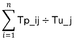

生産期間全体を通した目標生産率平均Apに対して、下記数式62を満たさない場合に、目標生産率や時間的制約(納期やQ-time制約など)を達成できない生産リスクが発生すると判定できる。

以上、最適な保全・段取り計画に基づく同時可動台数や稼働率により、適正な装置台数を算定することができ、設備計画の高精度化が可能となる。また、この装置台数を用いて行われる業務スケジュールは、実際の時間軸・設備運用条件下で実行可能であることが確認されており、実行可能性が高い。
次に、第12実施形態に係わる人員数量の計画方法を説明する。
上記(1)の同時期に停止する設備の数量と性能と、上記(2)の最適な多品種の生産順序と段取り時期によって、同時期に必要となる人員(設備エンジニアやプロセスエンジニア、オペレータ等)の最適数量を算定できる。
上記(1)の同時期に停止する設備の数量と性能と、上記(2)の最適な多品種の生産順序と段取り時期によって、同時期に必要となる人員(設備エンジニアやプロセスエンジニア、オペレータ等)の最適数量を算定できる。
実施形態6の最適指標生成方法から求められる生産期間Tcにおける段取り回数Ns、総段取り時間Ts、同時期に発生する保全数Ndとその時間長から、必要とされる人員数を算定していく。まず、同時期に停止する設備数Ndから、設備保全に関わる最小要員数が算定される。また、段取りプロセスの作業に必要な人員数は、人員要求率Ns/Tcおよび作業要求率Ts/Tcを用いて算定する。人員の勤務時間や休憩時間を考慮した人員実効作業率Uoに対して、Nop×Ts/Tc<Uoの条件を満たす最大の人員数Nop*を基本人員数として算定する。
ここで、通常、段取り作業を行う人員は、複数の装置やプロセスを管理対象としていることが多い。段取りプロセスの作業に必要な人員数の算定においても、同時期に複数の異なる段取り作業が発生する場合には、必要人員数を追加する。なお、半導体産業などの設備投資が製造コストの半分以上を占める産業では、人員数が少ないことによって設備を止めることのないように人員計画されることが多い。
設備と人員の計画に共通して、上記(3)段取り時間を活用して設備の保全時期を分散化する装置対品種割り当て(以下、第2次割当て)と保全順序を算定する前に、段取り時間低減と生産リスク低減および良品率向上の多目的での生産設備の使用条件・処理品種の限定(以下、第1次割当て)を決定する。ここで、段取り最小化のためには、専用装置を最大限に増やし、共用装置台数を最小限に抑える。また、一方で、生産リスク最少化のためには、製品品種を処理可能な装置台数を最大限に増やし、結果的に共用装置台数を最大限に増やすことになる。現実の第一次装置割り当てでは、必要装置台数に1以上の値を加えるなどしている。第1次割当ては、企業各社の方針・方法に依存するが、特定装置と特定製品品種の割当が複雑に設定されている場合(例えば、図22)でも、第12実施形態の設備人員計画方法は使用可能である。
<第13実施形態>
まず、第7実施形態と第12実施形態の問題点について説明する。
第7実施形態では、管理対象とする生産工程の全ての装置群についてJAMP-wS法により算定される保全や段取り時期に寄り発生する静的生産スパイクに動的な故障などを合わせた動的生産スパイクを複数の生産工程について重ね合わせて複合スパイクを分析し、対象とする生産工程のスパイクを最小の安全在庫で吸収する方法を示した。しかし、その最適指標生成方法は、設備・人員・仕掛り品の最適運用を示すに留まっていた。また、第12実施形態では、第6実施形態の応用によって設備人員計画の高精度化や生産計画の実行可能性向上を実現する変形例を示した。しかし、第12実施形態には、動的に発生する装置の突発故障等の対応を明示的に扱った技術ではなかった。
そこで、第13実施形態では、第7実施形態を応用して、第12実施形態に対して更に動的に発生する装置故障を考慮して、設備人員計画の高精度化や生産計画の実行可能性向上を実現し、コスト削減や利益向上を実現することを目的としている。
まず、第7実施形態と第12実施形態の問題点について説明する。
第7実施形態では、管理対象とする生産工程の全ての装置群についてJAMP-wS法により算定される保全や段取り時期に寄り発生する静的生産スパイクに動的な故障などを合わせた動的生産スパイクを複数の生産工程について重ね合わせて複合スパイクを分析し、対象とする生産工程のスパイクを最小の安全在庫で吸収する方法を示した。しかし、その最適指標生成方法は、設備・人員・仕掛り品の最適運用を示すに留まっていた。また、第12実施形態では、第6実施形態の応用によって設備人員計画の高精度化や生産計画の実行可能性向上を実現する変形例を示した。しかし、第12実施形態には、動的に発生する装置の突発故障等の対応を明示的に扱った技術ではなかった。
そこで、第13実施形態では、第7実施形態を応用して、第12実施形態に対して更に動的に発生する装置故障を考慮して、設備人員計画の高精度化や生産計画の実行可能性向上を実現し、コスト削減や利益向上を実現することを目的としている。
第13実施形態では、第7実施形態の故障監視・予測等に基づく装置の停止予定を加えて算定される同時停止装置台数の最大値をNdd(k)とすると、同時可動台数の最小値は(Mk-Ndd(k))となる。
本発明は、生産シミュレーション、生産スケジューリング、生産計画、設備人員計画、負荷計算などに利用でき、また、半導体・液晶産業のほか、情報通信業、卸売業、医療業などにも応用できる。
2 処理工程(装置群)、3 処理工程(装置群)、4 バッファサイズ、10 生産管理システム、11 最適指標生成装置、12 入力部、12A 入力モジュール、13 補助入力部、14 Q-time構造分析部、15 CKB最適論理値計算部、16 感度解析部(CKB特性)、17 指標算出部、18 感度解析部(性能特性)、19 最適ロードルール判定部、21 最適指標生成装置、22 入力部、22A 入力モジュール、23 補助入力部、24 JAMP最適論理値計算部、25 感度解析部(JAMP特性)、26 開始終了時期算出部、27 感度解析部(性能特性)、28 装置区分算定部、29 エンジニアリング業務システム、31 最適指標生成装置、32 変動監視検出部、33 入力変更検出部、34 再計算必要性判断部、35 感度解析部(CKB+JAMP特性)、36 CKB+JAMP最適論理値計算部、37 感度解析部(CKB+JAMP性能特性)、38 計算指示部、41 最適指標生成装置、42 生産フローボトルネック・流量解析部、43 Q-time構造分析部、44 装置区分算定部、45 補助入力部、46 駆動制御部、47 余裕時間配分解析部、51 最適指標生成装置、52 補助入力部(JAMP-wS法)、53 段取り替えサイクル算定部、54 装置区分算定部、55 JAMP-wS最適論理値計算部、56 開始終了時期算出部、57 感度解析部(性能特性)、58 感度解析部(JAMP特性)、61 最適指標生成装置、62 補助入力部(CKB=JAMP-wS2法)、63 装置群生産周期位相設定部、64 生産スパイク算定部、65 CKB=JAMP-wS2最適理論値計算部、66 指標算出部、67 感度解析部(CKB=JAMP-wS2性能特性)、68 感度解析部(CKB=JAMP-wS2特性)、71 最適指標生成装置、72 最適指標生成成装置61計算モジュール、73 最適指標生成成装置41計算モジュール、76 指標算出部
Claims (33)
- 多品種の製品を生産するため複数の装置を制御する生産管理システムに対して、前記複数の装置と製品に関する指標情報を供給する最適指標生成装置であって、
前記複数の装置と製品に関する情報を前記生産管理システムを介して入力する情報入力部と、
前記入力された情報から前記複数の装置による加工工程間の滞在時間の制限値を示すQ-time構造を分析するQ-time構造分析部と、
前記入力された情報および前記Q-time構造に基づいて、品種別の最適なカンバン枚数およびバッファサイズを計算する最適理論値計算部と、
前記計算された情報を指標情報として出力する指標算出部と、
製品の到着に関連するバッチ組み待ち時間とQ-time制約の上限値との大小関係が切り替わる到着率の境界値を算定し、適切なロードルールを判定する最適ロードルール判定部と、を備え、
前記指標算出部により算出された最適な指標情報とロードルールとを前記生産管理システムに供給することを特徴とする最適指標生成装置。
- 前記最適理論値計算部により算出された最適な指標情報に対して、感度解析を予め行っておく感度解析部と、
各種入力情報の変動に対応した最適な指標情報を即時に生産管理システムに供給する指標算出部と、をさらに備え、
前記指標算出部は、後続工程区間または先行工程区間のスループットの変化に連動してカンバン枚数やバッファサイズを変更することを特徴とする請求項1記載の最適指標生成装置。 - 多品種の製品を生産するため複数の装置を制御する生産管理システムに対して、前記複数の装置と製品に関する指標情報を供給する最適指標生成方法であって、
前記複数の装置と製品に関する情報を前記生産管理システムを介して入力する情報入力ステップと、
前記入力された情報から前記複数の装置による加工工程間の滞在時間の制限値を示すQ-time構造を分析するQ-time構造分析ステップと、
前記入力された情報および前記Q-time構造に基づいて、品種別の最適なカンバン枚数およびバッファサイズを計算する最適理論値計算ステップと、
前記計算された情報を指標情報として出力する指標算出ステップと、
製品の到着に関連するバッチ組み待ち時間とQ-time制約の上限値との大小関係が切り替わる到着率の境界値を算定し、適切なロードルールを判定する最適ロードルール判定ステップと、を実行し、
前記指標算出ステップにより算出された最適な指標情報とロードルールとを前記生産管理システムに供給することを特徴とする最適指標生成方法。 - 前記最適理論値計算ステップにより算出された最適な指標情報に対して、感度解析を予め行っておく感度解析ステップと、
各種入力情報の変動に対応した最適な指標情報を即時に生産管理システムに供給する指標算出ステップをさらに行うことを特徴とする請求項3記載の最適指標生成方法。 - 前記指標算出ステップは、後続工程区間または先行工程区間のスループットの変化に連動してカンバン枚数やバッファサイズを変更することを特徴とする請求項3記載の最適指標生成方法。
- 前記指標算出ステップは、前記加工工程間で待つことが可能な最大ロット数を超えないように、前記複数の装置による加工工程間に設けられたバッファのサイズを制限することにより、先行工程の製品の出力を制御することを特徴とする請求項3記載の最適指標生成方法。
- 前記Q-time制約区間内のボトルネック箇所のトラフィック強度が1を超えないように制御することを特徴とする請求項3記載の最適指標生成方法。
- 前記トラフィック強度が1より大きくなる場合には、トラフィック強度が1になるようにQ-time制約区間へのロットの投入率を制御することを特徴とする請求項3記載の最適指標生成方法。
- 前記Q-time制約区間内に滞在するロットの数を製品品種および処理条件別のカンバン枚数によって制限し、各ロットの処理開始時期を空きカンバンによって制御することを特徴とする請求項3記載の最適指標生成方法。
- 請求項3乃至9の何れか1項記載の最適指標生成方法におけるステップをプロセッサに実行させることを特徴とする最適指標生成プログラム。
- 多品種の製品を生産するため複数の装置を制御する生産管理システムに対して、通信回線を介して前記複数の装置と製品に関する指標情報を送信する最適指標生成サーバであって、
前記複数の装置と製品に関する情報を前記生産管理システムを介して受信する情報受信部と、
前記受信された情報から前記複数の装置による加工工程間の滞在時間の制限値を示すQ-time構造を分析するQ-time構造分析部と、
前記受信された情報および前記Q-time構造に基づいて、品種別の最適なカンバン枚数およびバッファサイズを計算する最適理論値計算部と、
前記計算された情報を指標情報として出力する指標算出部と、
製品の到着に関連するバッチ組み待ち時間とQ-time制約の上限値との大小関係が切り替わる到着率の境界値を算定し、適切なロードルールを判定する最適ロードルール判定部と、を備え、
前記指標算出部により算出された最適な指標情報とロードルールとを前記生産管理システムに送信することを特徴とする最適指標生成サーバ。 - 多品種の製品を生産するため複数の装置を制御する生産管理システムに対して、通信回線を介して前記複数の装置と製品に関する指標情報を送信するサーバが実行する最適指標生成方法であって、
前記複数の装置と製品に関する情報を前記生産管理システムを介して受信する情報受信ステップと、
前記受信された情報から前記複数の装置による加工工程間の滞在時間の制限値を示すQ-time構造を分析するQ-time構造分析ステップと、
前記受信された情報および前記Q-time構造に基づいて、品種別の最適なカンバン枚数およびバッファサイズを計算する最適理論値計算ステップと、
前記計算された情報を指標情報として出力する指標算出ステップと、
製品の到着に関連するバッチ組み待ち時間とQ-time制約の上限値との大小関係が切り替わる到着率の境界値を算定し、適切なロードルールを判定する最適ロードルール判定ステップと、を実行し、
前記指標算出ステップにより算出された最適な指標情報とロードルールとを前記生産管理システムに送信することを特徴とする最適指標生成方法。 - 多品種の製品を生産するための生産実行システムに設けられた複数の装置を制御する生産管理システムに対して、前記複数の装置に関する指標情報を供給する最適指標生成装置であって、
前記生産実行システムに含まれる複数の装置に関する情報を前記生産管理システムを介して入力する情報入力部と、
前記入力された情報から前記複数の装置による加工工程の中のボトルネック箇所および最大流量を解析するボトルネック箇所解析部と、
前記入力された情報から1つ以上のQ-time制約が存在しているQ-time制約区間の構造を分析するQ-time制約構造分析部と、
前記生産実行システムに含まれる複数の装置に関する情報を前記生産管理システムを介して入力する情報入力部と、
前記複数の装置を常用能力を有する常用装置と代替能力を有する代替装置とに区分する装置区分算定部と、
前記算定された装置区分と入力された情報から前記複数の常用装置と代替装置の稼働回数と稼働時期を算出する最適理論値計算部と、
前記常用装置と代替装置とに関する予防保全開始時期を算出する時間指標算出部と、
前記ボトルネック箇所、最大流量、前記Q-time構造および前記装置区分と前記時間指標に基づいて、品種別の最適なカンバン枚数およびバッファサイズを算出する最適理論値計算部と、
前記算出された最適理論値を指標情報として出力する指標算出部と、 前記生産実行システムに含まれる製造フロー全体に点在するすべてのQ-time制約を同時に管理する手続き実行制御部と、を備え、
前記時間指標算出部と指標算出部により算出された最適な指標情報を前記生産管理システムやエンジニアリング業務システムに供給するとともに、前記時間指標算出部により算出された最適な指標情報を生産管理システムに供給することを特徴とする最適指標生成装置。 - 多品種の製品を生産するための生産実行システムに設けられた複数の装置を制御する生産管理システムに対して、前記複数の装置に関する指標情報を供給する最適指標生成方法であって、
前記生産実行システムに含まれる複数の装置に関する情報を前記生産管理システムを介して入力する情報入力ステップと、
前記入力された情報から前記複数の装置による加工工程の中のボトルネック箇所および最大流量を解析するボトルネック箇所解析ステップと、
前記入力された情報から1つ以上のQ-time制約が存在しているQ-time制約区間の構造を分析するQ-time制約構造分析ステップと、
前記生産実行システムに含まれる複数の装置に関する情報を前記生産管理システムを介して入力する情報入力ステップと、
前記複数の装置を常用能力を有する常用装置と代替能力を有する代替装置とに区分する装置区分算定ステップと、
前記算定された装置区分と入力された情報から前記複数の常用装置と代替装置の稼働回数と稼働時期と稼動条件を算出する最適理論値計算ステップと、
前記常用装置と代替装置とに関する予防保全開始時期を算出する時間指標算出ステップと、
前記ボトルネック箇所、最大流量、前記Q-time構造および前記装置区分と時間指標に基づいて、品種別の最適なカンバン枚数およびバッファサイズを算出する最適理論値計算ステップと、
前記算出された最適理論値を指標情報として出力する指標算出ステップと、を実行し、
前記時間指標算出ステップと指標算出ステップにより算出された最適な指標情報を前記生産管理システムやエンジニアリング業務システムに供給するとともに、前記時間指標算出ステップにより算出された最適な指標情報を生産管理システムに供給することを特徴とする最適指標生成方法。 - 前記生産実行システムに含まれる製造フロー全体に点在するすべてのQ-time制約を同時に管理する手続き実行制御ステップをさらに行うことを特徴とする請求項14記載の最適指標生成方法。
- 前記生産実行システムに含まれる製造フロー全体における生産流量や工程能力の変動に対応してQ-time制約を同時に管理するために、製造フローにおけるボトルネック箇所と各工程の最大流量を解析する生産フローボトルネック・流量解析ステップをさらに行うことを特徴とする請求項14記載の最適指標生成方法。
- 請求項14乃至16の何れか1項記載の最適指標生成方法におけるステップをプロセッサに実行させることを特徴とする最適指標生成プログラム。
- 多品種の製品を生産するための生産実行システムに設けられた複数の装置を制御する生産管理システムに対して、通信回線を介して前記複数の装置に関する指標情報を送信する最適指標生成サーバであって、
前記生産実行システムに含まれる複数の装置に関する情報を前記生産管理システムを介して受信する情報受信部と、
前記受信された情報から前記複数の装置による加工工程の中のボトルネック箇所および最大流量を解析するボトルネック箇所解析部と、
前記受信された情報から1つ以上のQ-time制約が存在しているQ-time制約区間の構造を分析するQ-time制約構造分析部と、
前記生産実行システムに含まれる複数の装置に関する情報を前記生産管理システムを介して受信する情報受信部と、
前記複数の装置を常用能力を有する常用装置と代替能力を有する代替装置とに区分する装置区分算定部と、
前記算定された装置区分と受信された情報から前記複数の常用装置と代替装置の稼働回数と稼働時期と稼動条件を算出する最適理論値計算部と、
前記常用装置と代替装置とに関する予防保全開始時間を算出する時間指標算出部と、
前記ボトルネック箇所、最大流量、前記Q-time構造および前記装置区分と前記時間指標に基づいて、品種別の最適なカンバン枚数およびバッファサイズを算出する最適理論値計算部と、
前記算出された最適理論値を指標情報として出力する指標算出部と、を備え、
前記時間指標算出部と指標算出部により算出された最適な指標情報を前記生産管理システムやエンジニアリング業務システムに送信するとともに、前記時間指標算出部により算出された最適な指標情報を生産管理システムに送信することを特徴とする最適指標生成サーバ。 - 多品種の製品を生産するための生産実行システムに設けられた複数の装置を制御する生産管理システムに対して、通信回線を介して前記複数の装置に関する指標情報を送信するサーバが実行する最適指標生成方法であって、
前記生産実行システムに含まれる複数の装置に関する情報を前記生産管理システムを介して受信する情報受信ステップと、
前記受信された情報から前記複数の装置による加工工程の中のボトルネック箇所および最大流量を解析するボトルネック箇所解析ステップと、
前記受信された情報から1つ以上のQ-time制約が存在しているQ-time制約区間の構造を分析するQ-time制約構造分析ステップと、
前記ボトルネック箇所、最大流量および前記Q-time構造に基づいて、品種別の最適なカンバン枚数およびバッファサイズを計算して指標情報として出力する指標算出ステップと、
前記生産実行システムに含まれる複数の装置に関する情報を前記生産管理システムを介して受信する情報受信ステップと、
前記複数の装置を常用能力を有する常用装置と代替能力を有する代替装置とに区分する装置区分算定ステップと、
前記算定された装置区分と受信された情報から前記複数の常用装置と代替装置の稼働回数と稼働時期と稼動条件を算出する最適理論値計算ステップと、
前記常用装置と代替装置とに関する予防保全開始時間を算出する時間指標算出ステップと、を実行し、
前記指標算出ステップにより算出された最適な指標情報を前記生産管理システムやエンジニアリング業務システムに送信するとともに、前記時間指標算出ステップにより算出された最適な指標情報を生産管理システムに送信することを特徴とする最適指標生成方法。 - 多品種の製品を生産するための複数の装置を制御する生産管理システムに対して、前記複数の装置に関する指標情報を供給する最適指標生成装置であって、
前記複数の装置に関する情報を前記生産管理システムを介して入力する情報入力部と、
前記複数の装置を常用能力を有する常用装置と代替能力を有する代替装置とに区分する装置区分算定部と、
前記算定された装置区分と入力された情報から前記複数の常用装置と代替装置の稼働回数と稼働時期と稼動条件を算出する最適理論値計算部と、
前記計算出結果から前記常用装置と代替装置とに関する予防保全開始・終了時期を算出する開始終了時期算出部と、を備え、
前記開始終了時期算出部により算出された最適な開始終了時期情報を前記生産管理システムやエンジニアリング業務システムに供給することを特徴とする最適指標生成装置。 - 前記最適理論値計算部により算出された最適な開始終了時期情報に対して、感度解析を予め行っておく感度解析部と、
各種入力情報の変動に対応した最適な指標情報を即時に前記生産管理システムに供給する開始終了時期算出部をさらに備えることを特徴とする請求項20記載の最適指標生成装置。 - 多品種の製品を生産するための複数の装置を制御する生産管理システムに対して、前記複数の装置に関する指標情報を供給する最適指標生成方法であって、
前記複数の装置に関する情報を前記生産管理システムを介して入力する情報入力ステップと、
前記複数の装置を常用能力を有する常用装置と代替能力を有する代替装置とに区分する装置区分算定ステップと、
前記算定された装置区分と入力された情報から前記複数の常用装置と代替装置の稼働回数と稼働時期と稼動条件を算出する最適理論値計算ステップと、
前記計算出結果から前記常用装置と代替装置とに関する予防保全開始・終了時期を算出する開始終了時期算出ステップと、を実行し、
前記開始終了時期算出ステップにより算出された最適な開始終了時期情報を前記生産管理システムやエンジニアリング業務システムに供給することを特徴とする最適指標生成方法。 - 前記最適理論値計算ステップにより算出された最適な開始終了時期情報に対して、感度解析を予め行っておく感度解析ステップと、
各種入力情報の変動に対応した最適な指標情報を即時に前記生産管理システムに供給する開始終了時期算出ステップとをさらに行うことを特徴とする請求項8記載の最適指標生成方法。 - 請求項22または23記載の最適指標生成方法におけるステップをプロセッサに実行させることを特徴とする最適指標生成プログラム。
- 多品種の製品を生産するための複数の装置を制御する生産管理システムに対して、通信回線を介して前記複数の装置に関する指標情報を送信する最適指標生成サーバであって、
前記複数の装置に関する情報を前記生産管理システムを介して受信する情報入力部と、
前記複数の装置を常用能力を有する常用装置と代替能力を有する代替装置とに区分する装置区分算定部と、
前記算定された装置区分と入力された情報から前記複数の常用装置と代替装置の稼働回数と稼働時期と稼動条件を算出する最適理論値計算部と、
前記計算出結果から前記常用装置と代替装置とに関する予防保全開始・終了時期を算出する開始終了時期算出部と、を備え、
前記開始終了時期算出部により算出された最適な開始終了時期情報を前記生産管理システムやエンジニアリング業務システムに送信することを特徴とする最適指標生成サーバ。 - 多品種の製品を生産するための複数の装置を制御する生産管理システムに対して、通信回線を介して前記複数の装置に関する指標情報を送信するサーバが実行する最適指標生成方法であって、
前記複数の装置に関する情報を前記生産管理システムを介して受信する情報受信ステップと、
前記複数の装置を常用能力を有する常用装置と代替能力を有する代替装置とに区分する装置区分算定ステップと、
前記算定された装置区分と受信された情報から前記複数の常用装置と代替装置の稼働回数と稼働時期と稼動条件を算出する最適理論値計算ステップと、
前記計算出結果から前記常用装置と代替装置とに関する予防保全開始・終了時期を算出する開始終了時期算出ステップと、を実行し、
前記開始終了時期算出ステップにより算出された最適な開始終了時期情報を前記生産管理システムやエンジニアリング業務システムに送信することを特徴とする最適指標生成方法。 - 多品種の製品を生産するための生産実行システムに設けられた複数の装置を制御する生産管理システムに対して、前記複数の装置に関する指標情報を供給する最適指標生成装置であって、
前記生産実行システムに含まれる複数の装置に関する情報を生産管理システムを介して入力する情報入力部と、
前記入力された情報から前記複数の装置による加工工程間の滞在時間の制限値を示すQ-time制約を分析するQ-time構造分析部と、
前記生産実行システムに含まれる複数の装置に関する情報を生産管理システムから入力する情報入力部と、
前記複数の装置を常用能力を有する常用装置と代替能力を有する代替装置とに区分する装置区分算定部と、
前記算定された装置区分と入力された情報から前記複数の常用装置と代替装置の稼働回数と稼働時期と稼動条件を算出する最適理論値計算部と、
前記常用装置と代替装置とに関する予防保全開始時間を算出する開始終了時期算出部と、
前記入力された情報、前記Q-time構造および前記装置区分と前記開始終了時期に基づいて、品種別の最適なカンバン枚数およびバッファサイズを算出する最適理論値計算部と、
前記算出された最適理論値を指標情報として出力する指標算出部と、を備え、
前記開始終了時期算出部により算出された最適な開始終了時期情報を前記生産管理システムやエンジニアリング業務システムに供給するとともに、前記算出された開始終了時期により定まる工程能力が異なる各期に対して最適な指標情報を最適理論値計算部および前記指標算出部により生産管理システムに供給することを特徴とする最適指標生成装置。 - 前記指標算出部および前記開始終了時期算出部により算出された最適な指標情報および開始終了時期に対して、感度解析を予め行っておく感度解析部と、各種入力情報の変動に対応した最適な指標情報および開始終了時期情報を即時に前記生産管理システムに供給する開始終了時期算出部とをさらに備えることを特徴とする請求項27記載の最適指標生成装置。
- 多品種の製品を生産するための生産実行システムに設けられた複数の装置を制御する生産管理システムに対して、前記複数の装置に関する指標情報を供給する最適指標生成方法であって、
前記生産実行システムに含まれる複数の装置に関する情報を生産管理システムを介して入力する情報入力ステップと、
前記入力された情報から前記複数の装置による加工工程間の滞在時間の制限値を示すQ-time制約を分析するQ-time構造分析ステップと、
前記生産実行システムに含まれる複数の装置に関する情報を生産管理システムから入力する情報入力ステップと、
前記複数の装置を常用能力を有する常用装置と代替能力を有する代替装置とに区分する装置区分算定ステップと、
前記算定された装置区分と入力された情報から前記複数の常用装置と代替装置の稼働回数と稼働時期と稼動条件を算出する最適理論値計算ステップと、
前記常用装置と代替装置とに関する予防保全開始時間を算出する開始終了時期算出ステップと、
前記入力された情報、前記Q-time構造および前記装置区分と前記開始終了時期基づいて、品種別の最適なカンバン枚数およびバッファサイズを算出する最適理論値計算ステップと、
前記算出された最適理論値を指標情報として出力する指標算出ステップと、を実行し、
前記開始終了時期算出ステップにより算出された最適な開始終了時期情報を前記生産管理システムやエンジニアリング業務システムに供給するとともに、前記算出された開始終了時期により定まる工程能力が異なる各期に対して最適な指標情報を最適理論値計算ステップおよび前記指標算出ステップにより生産管理システムに供給することを特徴とする最適指標生成方法。 - 前記指標算出ステップおよび前記開始終了時期算出ステップにより算出された最適な指標情報および開始終了時期に対して、感度解析を予め行っておく感度解析ステップと、
各種入力情報の変動に対応した最適な指標情報および開始終了時期情報を即時に前記生産管理システムに供給する開始終了時期算出ステップとをさらに行うことを特徴とする請求項29記載の最適指標生成方法。 - 請求項29または30記載の最適指標生成方法におけるステップをプロセッサに実行させることを特徴とする最適指標生成プログラム。
- 多品種の製品を生産するための生産実行システムに設けられた複数の装置を制御する生産管理システムに対して、通信回線を介して前記複数の装置に関する指標情報を送信する最適指標生成サーバであって、
前記生産実行システムに含まれる複数の装置に関する情報を生産管理システムを介して受信する情報受信部と、
前記受信された情報から前記複数の装置による加工工程間の滞在時間の制限値を示すQ-time制約を分析するQ-time構造分析部と、
前記生産実行システムに含まれる複数の装置に関する情報を生産管理システムから受信する情報受信部と、
前記複数の装置を常用能力を有する常用装置と代替能力を有する代替装置とに区分する装置区分算定部と、
前記算定された装置区分と受信された情報から前記複数の常用装置と代替装置の稼働回数と稼働時期と稼動条件を算出する最適理論値計算部と、
前記常用装置と代替装置とに関する予防保全開始時間を算出する開始終了時期算出部と、
前記受信された情報、前記Q-time構造および前記装置区分と前記開始終了時期に基づいて、品種別の最適なカンバン枚数およびバッファサイズを算出する最適理論値計算部と、
前記算出された最適理論値を指標情報として出力する指標算出部と、を備え、
前記開始終了時期算出部により算出された最適な開始終了時期情報を前記生産管理システムやエンジニアリング業務システムに送信するとともに、前記算出された開始終了時期により定まる工程能力が異なる各期に対して最適な指標情報を最適理論値計算部および前記指標算出部により生産管理システムに送信することを特徴とする最適指標生成サーバ。 - 多品種の製品を生産するための生産実行システムに設けられた複数の装置を制御する生産管理システムに対して、通信回線を介して前記複数の装置に関する指標情報を送信するサーバが実行する最適指標生成方法であって、
前記生産実行システムに含まれる複数の装置に関する情報を生産管理システムを介して受信する情報受信ステップと、
前記受信された情報から前記複数の装置による加工工程間の滞在時間の制限値を示すQ-time制約を分析するQ-time構造分析ステップと、
前記受信された情報および前記Q-time構造に基づいて、品種別の最適なカンバン枚数およびバッファサイズを計算して指標情報として出力する指標算出ステップと、
前記生産実行システムに含まれる複数の装置に関する情報を生産管理システムから受信する情報受信ステップと、
前記複数の装置を常用能力を有する常用装置と代替能力を有する代替装置とに区分する装置区分算定ステップと、
前記算定された装置区分と受信された情報から前記複数の常用装置と代替装置の稼働回数と稼働時期と稼動条件を算出する最適理論値計算ステップと、
前記常用装置と代替装置とに関する予防保全開始時間を算出する開始終了時期算出ステップと、を実行し、
前記開始終了時期算出ステップにより算出された最適な開始終了時期情報を前記生産管理システムやエンジニアリング業務システムに送信するとともに、前記算出された開始終了時期により定まる工程能力が異なる各期に対して最適な指標情報を最適理論値計算ステップおよび前記指標算出ステップにより生産管理システムに送信することを特徴とする最適指標生成方法。
Applications Claiming Priority (2)
| Application Number | Priority Date | Filing Date | Title |
|---|---|---|---|
| JP2012148004A JP6044977B2 (ja) | 2011-06-30 | 2012-06-29 | 最適指標生成装置、最適指標生成方法、最適指標生成プログラム及び最適指標生成サーバ |
| JP2012-148004 | 2012-06-29 |
Publications (1)
| Publication Number | Publication Date |
|---|---|
| WO2014002319A1 true WO2014002319A1 (ja) | 2014-01-03 |
Family
ID=49784147
Family Applications (1)
| Application Number | Title | Priority Date | Filing Date |
|---|---|---|---|
| PCT/JP2012/084031 Ceased WO2014002319A1 (ja) | 2012-06-29 | 2012-12-28 | 最適指標生成装置、最適指標生成方法、最適指標生成プログラム及び最適指標生成サーバ |
Country Status (3)
| Country | Link |
|---|---|
| JP (1) | JP6044977B2 (ja) |
| TW (1) | TWI594100B (ja) |
| WO (1) | WO2014002319A1 (ja) |
Cited By (7)
| Publication number | Priority date | Publication date | Assignee | Title |
|---|---|---|---|---|
| WO2018179273A1 (ja) * | 2017-03-30 | 2018-10-04 | 日本電気株式会社 | フロー制御システム及びその制御方法 |
| CN111919183A (zh) * | 2018-05-10 | 2020-11-10 | 应用材料公司 | 用于排程半导体后端工厂的方法 |
| CN113359648A (zh) * | 2021-07-01 | 2021-09-07 | 哈尔滨理工大学 | 相同设备上虚拟调整时长的综合调度算法 |
| CN113935568A (zh) * | 2021-08-30 | 2022-01-14 | 国网江苏省电力有限公司物资分公司 | 一种在生产力恢复阶段制定采购策略的辅助决策方法 |
| CN114444948A (zh) * | 2022-01-28 | 2022-05-06 | 上海华力微电子有限公司 | 一种晶圆生产线智能获取派工wph的控制系统和方法 |
| CN116777192A (zh) * | 2023-08-23 | 2023-09-19 | 成都飞机工业(集团)有限责任公司 | 一种装配生产线动态排程方法 |
| US12314898B2 (en) * | 2019-08-28 | 2025-05-27 | Logisteed, Ltd. | Work planning system and work planning method |
Families Citing this family (9)
| Publication number | Priority date | Publication date | Assignee | Title |
|---|---|---|---|---|
| JP7261639B2 (ja) * | 2019-03-29 | 2023-04-20 | 川崎重工業株式会社 | 生産管理システム及び生産管理方法 |
| JP7339033B2 (ja) * | 2019-07-02 | 2023-09-05 | 株式会社ディスコ | 加工廃液処理装置の設置方法 |
| US12287624B2 (en) * | 2020-07-27 | 2025-04-29 | Applied Materials, Inc. | Time constraint management at a manufacturing system |
| JP7548666B2 (ja) * | 2020-09-23 | 2024-09-10 | 東京エレクトロン株式会社 | 半導体製造装置、基板搬送方法及びプログラム |
| CN112270522A (zh) * | 2020-10-14 | 2021-01-26 | 广东博智林机器人有限公司 | 一种钢筋作业方法和系统 |
| JP7574761B2 (ja) * | 2021-08-12 | 2024-10-29 | 株式会社Sumco | 製造ラインの工程計画立案装置及び方法 |
| TWI844845B (zh) | 2022-04-25 | 2024-06-11 | 財團法人工業技術研究院 | 產線運作預測方法以及產線運作預測系統 |
| CN117471996A (zh) * | 2023-10-19 | 2024-01-30 | 南京鼎华智能系统有限公司 | 生产线信息交换系统以及生产线信息交换方法 |
| JP7762466B1 (ja) * | 2025-07-22 | 2025-10-30 | 株式会社シムトレック | 生産シミュレーションシステム、生産シミュレーション方法及びプログラム |
Citations (3)
| Publication number | Priority date | Publication date | Assignee | Title |
|---|---|---|---|---|
| JP2003022119A (ja) * | 2001-07-06 | 2003-01-24 | Japan Science & Technology Corp | 多品種生産システム及びその設計・運用方法、その設計・運用プログラム及びそのプログラムを記録した記録媒体 |
| JP2003108213A (ja) * | 2001-09-27 | 2003-04-11 | Matsushita Electric Ind Co Ltd | 自動管理システム |
| JP2008077370A (ja) * | 2006-09-21 | 2008-04-03 | Renesas Technology Corp | 生産管理システムおよび生産管理方法 |
Family Cites Families (5)
| Publication number | Priority date | Publication date | Assignee | Title |
|---|---|---|---|---|
| US5612886A (en) * | 1995-05-12 | 1997-03-18 | Taiwan Semiconductor Manufacturing Company Ltd. | Method and system for dynamic dispatching in semiconductor manufacturing plants |
| US6738682B1 (en) * | 2001-09-13 | 2004-05-18 | Advances Micro Devices, Inc. | Method and apparatus for scheduling based on state estimation uncertainties |
| JP2004021856A (ja) * | 2002-06-19 | 2004-01-22 | World:Kk | フロー管理システム、フロー管理方法、並びにコンピュータ上で動作する情報処理プログラム |
| US7269469B2 (en) * | 2004-03-09 | 2007-09-11 | Taiwan Semiconductor Manufacturing Company, Ltd. | System and method for scheduling manufacturing jobs for a semiconductor manufacturing tool |
| CN100386702C (zh) * | 2005-06-10 | 2008-05-07 | 同济大学 | 基于信息素的用于半导体生产线的动态调度方法 |
-
2012
- 2012-06-29 JP JP2012148004A patent/JP6044977B2/ja active Active
- 2012-12-28 TW TW101151072A patent/TWI594100B/zh active
- 2012-12-28 WO PCT/JP2012/084031 patent/WO2014002319A1/ja not_active Ceased
Patent Citations (3)
| Publication number | Priority date | Publication date | Assignee | Title |
|---|---|---|---|---|
| JP2003022119A (ja) * | 2001-07-06 | 2003-01-24 | Japan Science & Technology Corp | 多品種生産システム及びその設計・運用方法、その設計・運用プログラム及びそのプログラムを記録した記録媒体 |
| JP2003108213A (ja) * | 2001-09-27 | 2003-04-11 | Matsushita Electric Ind Co Ltd | 自動管理システム |
| JP2008077370A (ja) * | 2006-09-21 | 2008-04-03 | Renesas Technology Corp | 生産管理システムおよび生産管理方法 |
Cited By (12)
| Publication number | Priority date | Publication date | Assignee | Title |
|---|---|---|---|---|
| WO2018179273A1 (ja) * | 2017-03-30 | 2018-10-04 | 日本電気株式会社 | フロー制御システム及びその制御方法 |
| JPWO2018179273A1 (ja) * | 2017-03-30 | 2019-11-21 | 日本電気株式会社 | フロー制御システム及びその制御方法 |
| US11385625B2 (en) | 2017-03-30 | 2022-07-12 | Nec Corporation | Flow control system and control method therefor |
| CN111919183A (zh) * | 2018-05-10 | 2020-11-10 | 应用材料公司 | 用于排程半导体后端工厂的方法 |
| US12314898B2 (en) * | 2019-08-28 | 2025-05-27 | Logisteed, Ltd. | Work planning system and work planning method |
| CN113359648A (zh) * | 2021-07-01 | 2021-09-07 | 哈尔滨理工大学 | 相同设备上虚拟调整时长的综合调度算法 |
| CN113359648B (zh) * | 2021-07-01 | 2022-12-09 | 哈尔滨理工大学 | 相同设备上虚拟调整时长的综合调度方法 |
| CN113935568A (zh) * | 2021-08-30 | 2022-01-14 | 国网江苏省电力有限公司物资分公司 | 一种在生产力恢复阶段制定采购策略的辅助决策方法 |
| CN113935568B (zh) * | 2021-08-30 | 2024-11-01 | 国网江苏省电力有限公司物资分公司 | 一种在生产力恢复阶段制定采购策略的辅助决策方法 |
| CN114444948A (zh) * | 2022-01-28 | 2022-05-06 | 上海华力微电子有限公司 | 一种晶圆生产线智能获取派工wph的控制系统和方法 |
| CN116777192A (zh) * | 2023-08-23 | 2023-09-19 | 成都飞机工业(集团)有限责任公司 | 一种装配生产线动态排程方法 |
| CN116777192B (zh) * | 2023-08-23 | 2023-12-08 | 成都飞机工业(集团)有限责任公司 | 一种装配生产线动态排程方法 |
Also Published As
| Publication number | Publication date |
|---|---|
| JP2013033466A (ja) | 2013-02-14 |
| JP6044977B2 (ja) | 2016-12-14 |
| TW201401001A (zh) | 2014-01-01 |
| TWI594100B (zh) | 2017-08-01 |
Similar Documents
| Publication | Publication Date | Title |
|---|---|---|
| JP6044977B2 (ja) | 最適指標生成装置、最適指標生成方法、最適指標生成プログラム及び最適指標生成サーバ | |
| Chung et al. | A modified genetic algorithm approach for scheduling of perfect maintenance in distributed production scheduling | |
| Li et al. | Process scheduling under uncertainty: Review and challenges | |
| Ni et al. | Decision support systems for effective maintenance operations | |
| JP2013033466A5 (ja) | ||
| Babaeimorad et al. | An integrated optimization of production and preventive maintenance scheduling in industry 4.0 | |
| CN112561177A (zh) | 一种产线均衡优化调度管理平台 | |
| Ren et al. | An Edge-Fog-Cloud Computing-Based Digital Twin Model for Prognostics Health Management of Process Manufacturing Systems. | |
| Yuniawan et al. | Overall equipment effectiveness estimation for priority improvement in the production line | |
| Fu et al. | Batch production scheduling for semiconductor back-end operations | |
| Chen et al. | Hybrid flow shop rescheduling algorithm for perishable products subject to a due date with random invalidity to the operational unit | |
| CN117557232A (zh) | 一种基于生产计划的高级排程方法 | |
| Chin et al. | Short Term Maintenance Tasks Scheduling with Pinch Methodology. | |
| Agarwal et al. | Flowshop Scheduling Problem for 10-Jobs, 10-Machines By Heuristics Models Using Makespan Criterion | |
| Rabbani et al. | Designing an advanced available-to-promise mechanism compatible with the make-to-forecast production systems through integrating inventory allocation and job shop scheduling with due dates and weighted earliness/tardiness cost | |
| Özbayrak et al. | How successfully does JIT handle machine breakdowns in an automated manufacturing system? | |
| Montororing | Model of flow shop scheduling problems considering multi-item testing operations multiple due dates and sequence dependent setup times | |
| Abogrean et al. | Integrated maintenance and cost optimisation of Libyan cement factory using witness simulation | |
| Bakhshi-Khanik et al. | Two-Stage Stochastic Programming for a Reconfigurable Unrelated Parallel Machine Scheduling Problem | |
| Abdullah et al. | Capacitated lot-sizing and scheduling with sequence-dependent setups in petrochemical plants | |
| Badr et al. | An agent-based approach for automating the disturbance handling for flexible manufacturing systems | |
| Pierce et al. | Value-based dispatching for semiconductor wafer fabrication | |
| Berkholz et al. | From volatile maintenance data forecasting to reliable capacity planning | |
| Fazlollahtabar et al. | Applying stochastic programming for optimizing production time and cost in an automated manufacturing system | |
| Bijari et al. | Integrated production planning model for noncyclic maintenance and production planning |
Legal Events
| Date | Code | Title | Description |
|---|---|---|---|
| 121 | Ep: the epo has been informed by wipo that ep was designated in this application |
Ref document number: 12880101 Country of ref document: EP Kind code of ref document: A1 |
|
| NENP | Non-entry into the national phase |
Ref country code: DE |
|
| 122 | Ep: pct application non-entry in european phase |
Ref document number: 12880101 Country of ref document: EP Kind code of ref document: A1 |