WO2004010872A1 - 超音波診断システム及び歪み分布表示方法 - Google Patents
超音波診断システム及び歪み分布表示方法 Download PDFInfo
- Publication number
- WO2004010872A1 WO2004010872A1 PCT/JP2003/009731 JP0309731W WO2004010872A1 WO 2004010872 A1 WO2004010872 A1 WO 2004010872A1 JP 0309731 W JP0309731 W JP 0309731W WO 2004010872 A1 WO2004010872 A1 WO 2004010872A1
- Authority
- WO
- WIPO (PCT)
- Prior art keywords
- compression
- correlation
- ultrasonic
- measurement point
- distribution
- Prior art date
Links
Classifications
-
- A—HUMAN NECESSITIES
- A61—MEDICAL OR VETERINARY SCIENCE; HYGIENE
- A61B—DIAGNOSIS; SURGERY; IDENTIFICATION
- A61B8/00—Diagnosis using ultrasonic, sonic or infrasonic waves
- A61B8/48—Diagnostic techniques
- A61B8/485—Diagnostic techniques involving measuring strain or elastic properties
-
- A—HUMAN NECESSITIES
- A61—MEDICAL OR VETERINARY SCIENCE; HYGIENE
- A61B—DIAGNOSIS; SURGERY; IDENTIFICATION
- A61B5/00—Measuring for diagnostic purposes; Identification of persons
- A61B5/0048—Detecting, measuring or recording by applying mechanical forces or stimuli
-
- A—HUMAN NECESSITIES
- A61—MEDICAL OR VETERINARY SCIENCE; HYGIENE
- A61B—DIAGNOSIS; SURGERY; IDENTIFICATION
- A61B8/00—Diagnosis using ultrasonic, sonic or infrasonic waves
- A61B8/08—Clinical applications
-
- A—HUMAN NECESSITIES
- A61—MEDICAL OR VETERINARY SCIENCE; HYGIENE
- A61B—DIAGNOSIS; SURGERY; IDENTIFICATION
- A61B8/00—Diagnosis using ultrasonic, sonic or infrasonic waves
- A61B8/48—Diagnostic techniques
- A61B8/488—Diagnostic techniques involving Doppler signals
-
- G—PHYSICS
- G01—MEASURING; TESTING
- G01S—RADIO DIRECTION-FINDING; RADIO NAVIGATION; DETERMINING DISTANCE OR VELOCITY BY USE OF RADIO WAVES; LOCATING OR PRESENCE-DETECTING BY USE OF THE REFLECTION OR RERADIATION OF RADIO WAVES; ANALOGOUS ARRANGEMENTS USING OTHER WAVES
- G01S15/00—Systems using the reflection or reradiation of acoustic waves, e.g. sonar systems
- G01S15/02—Systems using the reflection or reradiation of acoustic waves, e.g. sonar systems using reflection of acoustic waves
- G01S15/06—Systems determining the position data of a target
- G01S15/08—Systems for measuring distance only
- G01S15/10—Systems for measuring distance only using transmission of interrupted, pulse-modulated waves
-
- G—PHYSICS
- G01—MEASURING; TESTING
- G01S—RADIO DIRECTION-FINDING; RADIO NAVIGATION; DETERMINING DISTANCE OR VELOCITY BY USE OF RADIO WAVES; LOCATING OR PRESENCE-DETECTING BY USE OF THE REFLECTION OR RERADIATION OF RADIO WAVES; ANALOGOUS ARRANGEMENTS USING OTHER WAVES
- G01S15/00—Systems using the reflection or reradiation of acoustic waves, e.g. sonar systems
- G01S15/88—Sonar systems specially adapted for specific applications
- G01S15/89—Sonar systems specially adapted for specific applications for mapping or imaging
- G01S15/8906—Short-range imaging systems; Acoustic microscope systems using pulse-echo techniques
-
- G—PHYSICS
- G01—MEASURING; TESTING
- G01S—RADIO DIRECTION-FINDING; RADIO NAVIGATION; DETERMINING DISTANCE OR VELOCITY BY USE OF RADIO WAVES; LOCATING OR PRESENCE-DETECTING BY USE OF THE REFLECTION OR RERADIATION OF RADIO WAVES; ANALOGOUS ARRANGEMENTS USING OTHER WAVES
- G01S7/00—Details of systems according to groups G01S13/00, G01S15/00, G01S17/00
- G01S7/52—Details of systems according to groups G01S13/00, G01S15/00, G01S17/00 of systems according to group G01S15/00
- G01S7/52017—Details of systems according to groups G01S13/00, G01S15/00, G01S17/00 of systems according to group G01S15/00 particularly adapted to short-range imaging
- G01S7/52023—Details of receivers
- G01S7/52036—Details of receivers using analysis of echo signal for target characterisation
- G01S7/52042—Details of receivers using analysis of echo signal for target characterisation determining elastic properties of the propagation medium or of the reflective target
-
- A—HUMAN NECESSITIES
- A61—MEDICAL OR VETERINARY SCIENCE; HYGIENE
- A61B—DIAGNOSIS; SURGERY; IDENTIFICATION
- A61B8/00—Diagnosis using ultrasonic, sonic or infrasonic waves
- A61B8/08—Clinical applications
- A61B8/0825—Clinical applications for diagnosis of the breast, e.g. mammography
Definitions
- the present invention relates to an ultrasonic diagnostic system and a strain distribution display method capable of quantitatively measuring the hardness of a living tissue using an ultrasonic diagnostic apparatus.
- Ultrasonic tissue characterization is an application of medical ultrasound to measuring and imaging not only tissue shapes but also physical quantities such as sound velocity and attenuation constant in tissues using ultrasound.
- One of them is the field of measuring the hardness of tissue, that is, the elastic property, which is being actively studied. This is because the elastic properties of a tissue are closely related to its pathological state. For example, it is known that sclerosing cancers such as breast cancer and thyroid cancer, cirrhosis, and arteriosclerosis have harder lesions than normal tissues.
- sclerosing cancers such as breast cancer and thyroid cancer, cirrhosis, and arteriosclerosis have harder lesions than normal tissues.
- hardness information of living tissue was obtained by palpation, but it is difficult to express objective information by palpation, and it requires the experience of a doctor, and the measurable area is limited to a somewhat large lesion near the body surface .
- the ultrasonic echo signal (RF signal before compression) is measured before the tissue is compressed by the ultrasonic probe, using the ultrasonic diagnostic equipment and the ultrasonic probe as they are. 2 After that, the tissue is slightly compressed (about a few percent) with an ultrasonic probe, for example, and the ultrasonic echo signal (RF signal after compression) of the compressed tissue is measured. Then, from the measured RF signals before and after the tissue compression, the displacement distribution, which is the amount of displacement of each point inside the tissue due to compression, is estimated by the spatial correlation method.
- the spatial correlation method is a method of estimating the displacement distribution in the tissue caused by compression from the RF signal (or the envelope of the RF signal) before and after tissue compression by template matching using a two-dimensional correlation function.
- a fixed-size two-dimensional correlation window template
- This is a method of estimating that the measurement point of interest has moved to the two-dimensional position of the signal data by autocorrelation processing. This autocorrelation processing is performed for each measurement point set in a grid, for example, to estimate a displacement distribution.
- the sampling interval in the horizontal direction is generally larger than the sampling interval in the axial direction, so that the accuracy of the estimated displacement component is higher in the horizontal direction than in the axial direction.
- the spatial correlation method has a feature that a two-dimensional displacement vector component can be estimated.
- the displacement estimation accuracy is limited by the sampling interval, the displacement distribution can be estimated even when the tissue is significantly deformed (for example, about 5%).
- the amount of calculation required for the spatial correlation processing is enormous, which impairs the real-time property, which is an advantage of ultrasonic measurement.
- An object of the present invention is to obtain a displacement distribution, a strain distribution, and an elastic modulus distribution in real time.
- an ultrasonic diagnostic system of the present invention provides a displacement of tissue of a subject based on a reflected echo signal (RF signal) measured before and after compression of the subject by an ultrasound probe.
- the storage means for storing the feature quantity including the envelope signal of the RF signal output from the ultrasonic probe, and before and after compression based on the feature quantity of the subject stored before and after compression stored in this storage means
- Correlation calculating means for calculating the correlation coefficient of the characteristic amount of the above and the phase difference between the received signals before and after compression
- Displacement calculating means for calculating a displacement of a measurement point due to compression based on a relation number and a phase difference between RF signals before and after compression.
- the displacement of the measurement point is obtained by using the correlation based on the features such as the envelope signal before and after the compression, the displacement distribution can be estimated in real time.
- the problem of aliasing in the Doppler method can be solved.
- the self-time of the envelope signal after compression is shifted while shifting the time axis of the envelope signal after compression. If the correlation function is determined for each measurement point, the computation time may be too long and the real-time property may be impaired.
- the autocorrelation function of the envelope signal before and after compression is calculated first, and the obtained autocorrelation function is shifted according to the movement of the measurement point, for example, by a half wavelength interval of the ultrasonic signal, and the correlation coefficient is calculated. Is preferably obtained. As a result, the time required for the displacement calculation can be reduced, and the processing can be speeded up.
- the ultrasonic diagnostic system of the present invention further comprises: storage means for storing an envelope signal of the orthogonally detected RF signal; and the envelope before and after compression of the subject corresponding to the slice plane stored in the storage means.
- a measurement point is set in the frame data of the signal, the measurement point is moved at least two-dimensionally with respect to the frame data, and the envelope signal before and after the compression belonging to the two-dimensional correlation window surrounding the measurement point is compressed.
- a correlation calculating means for determining a position where the correlation coefficient is maximum, and a phase difference between the RF signals before and after the compression, a position where the correlation coefficient determined by the correlation calculating means is maximum, and A displacement calculating means for calculating a displacement of the measurement point in at least a two-dimensional direction due to the compression based on the phase difference.
- the two-dimensional direction is set to the direction of the ultrasonic beam received by the ultrasonic probe and the scanning direction of the ultrasonic beam.
- the moving pitch of the measurement point in the ultrasonic beam direction is not limited to a half wavelength interval of the ultrasonic signal, but a smaller pitch is preferable.
- the envelope before and after compression is obtained. It is desirable to find the autocorrelation function of the line signal, and to shift this autocorrelation function according to the movement of the measurement point to find the position where the correlation coefficient becomes maximum.
- the displacement calculation according to the present invention can be applied not only to two dimensions but also to three dimensions.
- frame data stored in the storage means is a multimedia data having frame data of a plurality of slice planes.
- an envelope signal obtained by scanning in the slice direction is added.
- the correlation calculating means moves the measurement point in the three-dimensional direction with respect to the polygon data, and determines a position where the correlation coefficient of the envelope signal before and after the compression belonging to the three-dimensional correlation window surrounding the measurement point is maximum. And the phase difference between the RF signals before and after compression.
- the three-dimensional directions are the direction of the ultrasonic beam received by the ultrasonic probe, the scanning direction of the ultrasonic beam, and the slice direction orthogonal to these.
- the correlation calculation means obtains a phase difference between the RF signals before and after the compression in the ultrasonic beam scanning direction, the ultrasonic beam scanning direction, and the slice direction orthogonal thereto.
- the above-described high-speed processing method can be applied also when obtaining a three-dimensional displacement.
- the method of obtaining the elastic modulus distribution is to divide the subject into a finite number of Also, it is possible to provide an elastic coefficient calculating means for creating a two-dimensional or three-dimensional finite element model and calculating an elastic coefficient distribution using the modeling information and the obtained strain distribution. Further, the obtained elasticity distribution can be displayed on the display means.
- the elastic modulus calculation means assumes that the subject tissue is an isotropic elastic body and near incompressible, divides the subject tissue into a finite number of rectangular parallelepiped elements, creates a three-dimensional finite element model, and It is preferable that the elastic modulus, stress, and strain are uniform, and the elastic modulus distribution is calculated using the strain distribution information in the elasticity equation.
- the assumption that the tissue is an isotropic elastic body is that when the tissue is statically compressed by applying external pressure, the relationship between stress and strain is almost linear, and the tissue is assumed to be an elastic body. Since the tissue can be approximated and the tissue of the subject is substantially isotropic, the present invention assumes that the tissue is an isotropic elastic body.
- Poisson's ratio 0.5
- the Poisson's ratio is a parameter that does not change much in the living body compared to the Young's modulus, it is preferable that the Poisson's ratio be constant at 0.49 in the present invention. According to this elastic modulus distribution calculation, the elastic modulus distribution can be reconstructed only from the axial strain distribution that can be calculated with high accuracy, and a stable elastic coefficient distribution can be calculated.
- FIG. 1 is a diagram for explaining the principle of an ultrasonic diagnostic apparatus.
- FIG. 2 is a diagram showing a specific example of a tissue elasticity measurement method using static compression and a principle of the tissue elasticity measurement method using static compression.
- FIG. 3 is a diagram illustrating the principle of the spatial correlation method.
- FIG. 4 is a diagram illustrating the principle of the Doppler method.
- FIG. 5 is a diagram illustrating the principle of the composite autocorrelation method.
- FIG. 6 shows a block diagram showing the circuit configuration that executes the basic algorithm of the complex autocorrelation method.
- FIG. 7 is a block diagram showing a schematic configuration of an ultrasonic diagnostic system according to one embodiment of the present invention.
- FIG. 8 is a flowchart showing a basic algorithm of the three-dimensional composite autocorrelation method.
- FIG. 9 is a flowchart showing a basic algorithm of the three-dimensional composite autocorrelation method according to the ultrasonic diagnostic system of the present invention, and is a flowchart showing details of a part of the processing of FIG.
- FIG. 10 is a flowchart showing details of the accelerated composite autocorrelation method in step S15 of FIG.
- FIG. 11 is a block diagram showing a circuit configuration for executing a basic algorithm of the three-dimensional composite autocorrelation method according to the ultrasonic diagnostic system of the present invention.
- FIG. 12 is a diagram schematically illustrating the procedure of the simulation.
- FIG. 13 is a diagram illustrating an example of each point spread function used when the ultrasonic center frequency is 5.0 MHz.
- Figure 14 is a diagram showing the outline of the organization model.
- FIG. 15 is a diagram illustrating a distortion estimation error of each method with respect to the lateral displacement.
- Figure 16 is a diagram showing the strain distribution estimated by each method (complex autocorrelation method, extended complex autocorrelation method, spatial correlation method) when the lateral displacement is 0.0 mm.
- Figure 17 is a diagram showing the strain distribution estimated by each method (combined autocorrelation method, extended combined autocorrelation method, spatial correlation method) when the lateral displacement is 0.4 mm.
- FIG. 18 is a diagram schematically showing a tissue model used for verification of oblique compression.
- Figure 19 shows the strain distribution estimation results when the tissue model is simply compressed in the axial direction.
- FIG. 20 shows a strain distribution estimation result when the tissue model is compressed in an oblique direction.
- FIG. 21 is a diagram showing an example of two tissue models having a three-dimensional structure.
- FIG. 22 is a first diagram illustrating each estimation result in the inclusion model.
- FIG. 23 is a second diagram illustrating each estimation result in the inclusion model.
- FIG. 24 is a first diagram illustrating each estimation result in the layered model.
- FIG. 25 is a second diagram illustrating each estimation result in the layered model.
- FIG. 26 is a diagram showing a basic configuration of the ultrasonic diagnostic system.
- FIG. 27 is a diagram showing a specific configuration of the ultrasonic scanner used in the ultrasonic diagnostic system. BEST MODE FOR CARRYING OUT THE INVENTION
- the ultrasonic diagnostic system of the present embodiment when performing the envelope correlation calculation, the processing that was one-dimensionally searched using the one-dimensional correlation window by the composite autocorrelation method is performed by performing a two-dimensional search using the two-dimensional correlation window.
- a method called the extended composite autocorrelation method that also supports lateral movement is adopted.
- this extended composite autocorrelation method reduces the amount of calculation by performing the envelope correlation calculation only at grid points at half-wavelength intervals in the axial direction and at line intervals in the horizontal direction, thereby increasing the speed. ing.
- the extended composite autocorrelation method also uses the phase information to improve the axial displacement estimation accuracy.
- phase information cannot be used for lateral displacement estimation because there is no signal to be used as a carrier. Therefore, the estimation accuracy of the lateral displacement is limited by the lateral sampling interval (ultrasonic beam line interval) as in the spatial correlation method.
- the elastic modulus distribution reconstruction method proposed later since the elastic modulus distribution can be estimated only from the axial strain (displacement) distribution, the lateral displacement estimation accuracy is not particularly improved in this embodiment.
- FIG. 1 is a diagram for explaining the principle of an ultrasonic diagnostic apparatus.
- the ultrasonic probe 10 as an ultrasonic probe converts an electric signal into an ultrasonic wave and converts the ultrasonic wave into an electric signal. Emit an ultrasonic pulse into tissue 11.
- the ultrasonic pulse radiated into the living tissue 11 is partially reflected at the first boundary 12 having a different acoustic impedance, and is reflected as a reflected echo 12 a. It goes to the wave probe 10 side, and the rest goes through.
- a part of the transmitted ultrasonic pulse is similarly reflected at the second boundary 13 having the next different acoustic impedance, travels to the ultrasonic probe 10 side as a reflected echo 13a, and the rest is transmitted.
- the reflected echo signal of the ultrasonic wave reflected in this way is received by the ultrasonic probe 10 and converted into a reflected echo signal of an electric signal.
- the time t from the emission of the ultrasonic pulse from the ultrasonic probe 10 to the reception of the reflected echo signal from the reflective object 14 (distance between different acoustic impedances) located at the distance L is The following equation (1) is obtained.
- c is the speed of sound in the living body, which can be regarded as approximately constant at 1500 [m / sec] in soft tissue. Therefore, by measuring the time t until the reflected echo signal is received, the distance L from the probe to the reflecting object can be obtained. Since the reflected echo signal has acoustic characteristic information of the living tissue, information of the living tissue such as a B-mode tomographic image can be displayed on the display based on the reflected echo signal. For example, using an ultrasonic diagnostic apparatus, an elastic property relating to the hardness of a tissue is measured.
- the principle of measuring elastic properties is to apply mechanical vibration to tissue and evaluate hardness information from the propagation speed of the shear wave.
- the propagation speed of the shear wave is faster in hard tissue and the propagation speed of the shear wave in soft tissue. Is based on being slow.
- the propagation velocity V of the transverse wave propagating through the living tissue is, as shown in the following formula (2), the tissue density P, the shear elastic modulus ⁇ , the shear viscosity coefficient 2 , and the angular frequency ⁇ of the vibration. Involved.
- FIG. 2A is a diagram showing a specific example of a tissue elasticity measurement method using static compression.
- Fig. 2 (B) is a diagram showing the principle of the tissue elasticity measurement method using static compression. As is clear from the figure, this method measures the ultrasonic echo signal (compressed RF signal) of the tissue 11 before compression using the conventional ultrasonic diagnostic apparatus and ultrasonic probe 10 as they are.
- the tissue 11 is slightly compressed (about several percent) by the ultrasonic probe 10, and the compressed ultrasonic echo signal (compressed RF signal) of the tissue 11 is measured. Then, from the measured RF signals before and after the tissue compression, a displacement distribution, which is the amount of movement of each point in the tissue due to the compression, is estimated.
- the main methods of this displacement distribution estimation method include a method using spatial correlation and a method using Doppler principle.
- FIG. 3 is a diagram illustrating the principle of the spatial correlation method.
- the displacement distribution inside the tissue caused by compression is estimated from the RF signal (or the envelope of the RF signal) before and after tissue compression by template matching using a two-dimensional correlation function.
- the specific processing is as follows. First, assuming that the RF signal (or its envelope signal) before and after tissue compression is (t, x), i 2 (t, x), the cross-correlation coefficient C (t, X; n, m) is given by the following equation (3).
- t is the coordinate in the ultrasonic beam direction (axial direction)
- X is the coordinate in the direction perpendicular to it (lateral direction)
- t Is the correlation window size in the axial direction
- x Q is the correlation window size in the horizontal direction
- Li is the sampling interval in the axial direction
- L x is the sampling interval in the horizontal direction
- n and m are integers.
- the accuracy of the estimated displacement component is lower in the lateral component than in the axial component.
- the above processing is performed for each measurement point to estimate the displacement distribution.
- the feature of the spatial correlation method is that it can estimate the two-dimensional displacement vector component.
- the displacement distribution can be estimated even when the tissue is greatly deformed (about 5%).
- the amount of calculation becomes enormous, the advantage of ultrasonic measurement, the real-time property, is lost.
- the displacement estimation accuracy is also limited by the sampling interval, there is a problem that the accuracy is lower than the Doppler method described later.
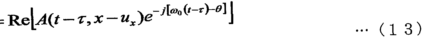
- FIG. 4 is a diagram illustrating the principle of the Doppler method. This method estimates the displacement distribution inside the tissue caused by compression from the RF signals before and after tissue compression using the Doppler principle used for blood flow measurement. The specific processing is as follows. First, the RF signal before and after tissue compression is modeled as in the following equation (4).
- the Doppler method is a method of estimating the displacement distribution by performing the above processing for each measurement point, and is the same processing as blood flow measurement based on the Doppler principle. Therefore, there is an advantage that real-time measurement is possible. Also, since the phase information is used, the displacement estimation accuracy is better than the spatial correlation method. However, when the amount of movement inside the tissue is large, for example, when the wavelength is more than a quarter wavelength of the ultrasonic center frequency, aliasing occurs and correct displacement cannot be estimated. As can be seen from the above equation, only the axial displacement component can be estimated.
- FIG. 5 is a diagram showing the principle of the composite autocorrelation method proposed by the present inventors.
- the composite autocorrelation method solves the aliasing problem in the Doppler method by using the correlation based on the RF signal envelope.
- the specific processing is as follows.
- the RF signal before and after tissue compression is modeled as in the following equation, as in the case of the Doppler method.
- T is the period of the ultrasonic wave
- R A (t; r) is the self of the envelope.
- the correlation function, t is the size of the correlation window
- * is the complex conjugate
- n is the number of movement pitches of the measurement points during the search
- R u (t; 0) is the autocorrelation function of (t)
- R 22 (t; n) is the autocorrelation function of s 2 (t + ⁇ ../ 2).
- the method of estimating the displacement distribution by performing the above processing for each measurement point is the composite autocorrelation method, which is an extended version of the Doppler method. Therefore, it is a method that enables real-time measurement.
- envelope correlation also supports displacement distribution estimation in the case of large deformation that cannot be measured by the Doppler method (when a displacement of more than one-quarter wavelength of ultrasonic waves occurs).
- FIG. 6 is a block diagram showing a circuit configuration for executing a basic algorithm of the composite autocorrelation method.
- the quadrature detection circuit (QD) 131 before pressurization inputs the signal before pressurization—the signal X (t), performs quadrature detection, and performs quadrature detection signals I x (t) and Qx (t).
- the signal is output to the first correlation operation circuit 133 and the first correlation coefficient operation circuits 1350 to 135N.
- the first correlation calculation circuit 133 calculates a correlation value RXX based on the signals Ix and Qx, and outputs it to each of the second correlation coefficient calculation circuits 1380 to 138N.
- the second correlation calculation circuit 1340 includes a quadrature detection signal I y (t), Qy (t) is input, a correlation value Ry y is calculated based on the signals I y and Qy, and the calculated value is output to the second correlation coefficient calculation circuit 1380.
- the first correlation coefficient calculation circuit 1350 includes a quadrature detection signal IX (t), Qx (t) from the quadrature detection circuit 131 before pressurization and a quadrature detection signal Iy (t) from the quadrature detection circuit 1320 after the first pressurization.
- Qy (t) are input to obtain complex baseband signals S R and S, which are output to the third correlation operation circuit 1360 and the phase difference operation circuit 1370.
- the third correlation operation circuit 1360 receives the complex baseband signals S R , S, from the first correlation coefficient operation circuit 1350, calculates a correlation value I Rxy I based on the complex base band signals S R , S, and calculates the second correlation coefficient Output to arithmetic circuit 1380.
- the phase difference calculation circuit 1370 receives the complex baseband signal S R , from the first correlation coefficient calculation circuit 1350, and calculates the phase difference ⁇ based on the signal. (T).
- the second phase relation number calculation circuit 1380 includes a correlation value R xx from the first correlation calculation circuit 133, a correlation value I Rxy I from the third correlation calculation circuit 1360, and a correlation value from the second correlation calculation circuit 1340. Enter Ry y and the correlation coefficient C based on each of these correlation values. Calculate (t) and output.
- (t) I y 1 + j Qy 1 outputs to the (I y, (t), Q yi (t)) of the first correlation coefficient computing circuit 1341 and the second correlation computing circuit 1351.
- the second correlation calculation circuit 1341 receives the quadrature detection signals I y, (t), Qy, (t) from the second quadrature detection circuit after pressurization (QD) 1321, and inputs the signals I y, (t), A correlation value Ry i is calculated based on Qy, (t) and output to the second correlation coefficient calculation circuit 1381.
- the first correlation coefficient calculation circuit 1351 is composed of the quadrature detection signals I x (t) and Qx (t) from the quadrature detection circuit 131 before compression, and the quadrature detection circuit (QD) 1321 from the second quadrature detection circuit after compression.
- the detection signals I y t (t), Qy, (t) are input, complex complex band signals S K1 , S n are obtained, and the signals are output to the third correlation operation circuit 1361 and the phase difference operation circuit 1371.
- the third correlation operation circuit 136 1 receives the complex baseband signals S R1 , S hinderfrom the first correlation coefficient operation circuit 1351, obtains a correlation value I Rxyi I based on the input, and calculates the second correlation coefficient Output to arithmetic circuit 1381.
- the second post-compression quadrature detection circuit (QD) 13 22 to 132N, the second correlation operation circuit 1342 to 134N, The correlation coefficient operation circuits 1352 to 135N, the third correlation operation circuits 1362 to 136N, the phase difference operation circuits 1 372 to 137N, and the second correlation coefficient operation circuits 1382 to 138N are the first and second stages described above.
- the same processing as that of the circuit group is performed, and the correlation coefficients C 2 (t) to C N (t) and the phases ⁇ 2 (t) to ⁇ ⁇ (t) are output.
- the circuit that executes the basic algorithm of the correlation method delays the pressurized echo signal y (t) by the delay circuit 134-13N by the ultrasonic cycle TZ2 (half wavelength), and then delays it by the quadrature detection circuit ( QD) Quadrature detection is individually performed using 1320 to 132N.
- the strain distribution can be obtained by spatially differentiating it.
- the strain distribution qualitatively represents the elastic properties of the tissue, and a diagnosis based on considerable elastic properties can be made even from the strain distribution.
- the entire lesion such as cirrhosis
- the tissue elastic modulus distribution is obtained from the strain distribution and stress distribution inside the tissue as described above.
- the elastic modulus distribution must be reconstructed in an inverse problem from the strain distribution and the boundary conditions for tissue compression. Therefore, it is generally difficult to solve the inverse problem, and few elastic modulus reconstruction methods have been proposed at present. A conventionally proposed elastic modulus reconstruction method will be described below.
- This method reconstructs the tissue elastic modulus distribution from the strain distribution (all components of the strain tensor including the shear strain component).
- estimating the absolute elastic modulus requires an area where the elastic modulus is known in advance (reference area).
- FIG. 7 is a block diagram showing a schematic configuration of an ultrasonic diagnostic system according to one embodiment of the present invention.
- an ultrasonic probe 91 transmits an ultrasonic wave into a subject and receives a reflected wave of the ultrasonic wave.
- a conventional sector scan probe sector phased array probe
- linear scan probe linear array
- Probe competing Scan probe
- RF signals before and after the tissue compression are output to the quadrature detector 92.
- the quadrature detector 92 converts the RF signal before and after the tissue compression into a complex envelope signal (IQ signal) before and after the tissue compression, respectively, and outputs the complex envelope signal to the complex two-dimensional correlation calculator 93.
- the complex two-dimensional correlation calculator 93 calculates the two-dimensional correlation between the RF signals before and after the tissue compression, and outputs the position where the correlation becomes maximum to the lateral displacement calculator 94 and the axial displacement calculator 95. Then, the phase of the correlation function at that time is output to the axial displacement calculator 95.
- Lateral displacement calculation unit 9 4 calculates the lateral displacement Iotaiota chi based on the correlation maximum position in the lateral direction from the complex two-dimensional correlation calculation unit 9 3, and outputs it to the lateral distortion calculation section 9 6 .
- the axial displacement calculator 9 5 calculates the displacement u y in the axial direction based on the axial direction of the correlation maximum position and phase at that time from the complex two-dimensional correlation calculation unit 9 3, axial strain it Output to calculation unit 97.
- the lateral distortion calculator 96 calculates the lateral distortion distribution ⁇ ⁇ ⁇ by spatially differentiating the distribution of the lateral displacement u x from the lateral displacement calculator 94 , and then quantizes it. Output to 8.
- axial strain calculating unit 9 7 calculates the axial strain distribution epsilon gamma by spatially differentiating the distribution of lateral displacement u y from axial displacement calculation unit 9 5, the quantization unit it Output to 9-8.
- Quantizer 9 8 each strain distribution transverse strain distribution epsilon chi and axial strain distribution epsilon gamma to grayscale (or color display) quantizes and outputs to the display unit 9 9.
- the display unit 99 displays each of the quantized distortion distributions.
- the RF signals before and after the tissue compression are first subjected to quadrature detection by the quadrature detector 92. That is, applying a sin wave and a cos wave having the same frequency as the center frequency of the ultrasonic wave to each RF signal and applying a low-pass filter to each of them gives a complex baseband signal s 2 as shown in the following equation (14). .
- T is the period of the ultrasonic wave
- L is the horizontal sampling interval (line interval)
- R A (t, X;, U x ) is the autocorrelation function of the envelope
- t Is the axial correlation window size
- X Is the horizontal correlation window size
- ⁇ is the shift amount of the integration in the time axis direction
- W is the shift amount of the integration in the beam line direction
- * represents the complex conjugate.
- R "(t, x; 0, 0) is s, (t, x) autocorrelation function
- R 22 (t, x; n, m) is s 2 (t + nT / 2 , x + mL
- the envelope correlation coefficient is used to overcome the aliasing problem in the same way as in the case of the composite autocorrelation method, that is, C (t) at each measurement point (t, X) , X; n, m) and a phase ⁇ C (t, ⁇ ; ⁇ , m), ⁇ (t,) of the phase ⁇ (t, ⁇ ; n, m) of R i2 (t, ⁇ ; ⁇ , m) ⁇ ; ⁇ , m) ⁇ for all ⁇ and m.
- ⁇ , because _kTZ2 I is smaller than ⁇ .
- ⁇ (t, X; k, 1) where no occurrence occurs the axial displacement u y and the lateral displacement ⁇ ⁇ can be expressed by the following formula (1) using the exact time shift at the measurement point (t, X). 1 7)
- c is the speed of sound in tissue (here, the typical speed of sound in soft tissue is 150 Om Zs). Therefore, if the axial displacement and the lateral displacement are calculated at all points in the tissue as described above, the axial displacement distribution u y (x, y) and the lateral displacement distribution u x (x, y) are obtained. can get.
- the above-mentioned extended composite autocorrelation method uses a two-dimensional correlation window and a search range so as to correspond to the lateral movement of the tissue, and the relative lateral direction of the tissue and the ultrasonic probe during tissue compression.
- displacement of tissue occurs in the direction perpendicular to the axial direction and the lateral direction (direction perpendicular to the two-dimensional ultrasonic scanning plane (slice direction)) during tissue compression.
- distortion cannot be estimated using the two-dimensional extended composite autocorrelation method. Therefore, in order to make the system more stable, it is possible to easily extend the extended composite autocorrelation method described above by using a three-dimensional correlation window and a three-dimensional search range.
- FIG. 9 and FIG. 10 are flowcharts showing the basic algorithm of the three-dimensional composite autocorrelation method.
- FIG. 10 is a flowchart showing details of a part of the process in FIG.
- step S11 in combination with the determination processing in step S23, "1" is stored in the scanning line number register 1 in order to perform the same processing from the first scanning line to the Lth scanning line. .
- step S12 a process of sequentially shifting the thickness direction (frame) from 1U to U is performed in combination with the determination process in step S18.
- step S13 a process of sequentially shifting the azimuth direction (scanning line) from 1V to V is executed in combination with the determination process in step S17.
- step S14 a process of sequentially shifting the distance direction (axial direction) from 0 to M is performed in combination with the determination process in step S16.
- step S15 the correlation coefficient C (1, t; u, V, n) of the envelope in the distance direction (axial direction) is calculated by the composite autocorrelation method.
- This composite autocorrelation method may be performed by a conventional method, but it takes a long time to calculate.
- the correlation coefficient C (1, t U, V, n) This high-speed composite autocorrelation method will be described later.
- Step S16 is a process combined with the previous step S14, in which it is determined whether or not the distance direction register n has reached its maximum value M. If so, the process proceeds to step S17. If not, the flow returns to step S14, and the distance direction register n is incremented.
- step S17 the process is combined with the previous step S13, and it is determined whether or not the direction register resistance V has reached its maximum value V. If so, the process proceeds to step S18. If not, the flow returns to step S13 to increment the azimuth direction register V.
- step S18 the process is combined with the previous step S12, and it is determined whether or not the thickness direction register u has reached its maximum value U. If so, the process proceeds to step S19. If not, the flow returns to step S12 to increment the thickness direction register u.
- step S 20 the correlation coefficient C (1 determined in step S 19, t;.
- step S23 the process is combined with the previous step S11, and it is determined whether or not the scanning line number register 1 has reached L. If so, the process proceeds to step S24, and so on. If not, the process returns to step S11, and the scan line number register 1 is incremented.
- step S24 when the displacement distribution due to the tissue compression is estimated, the strain distribution is calculated by spatially dividing it.
- FIG. 10 is a flowchart showing details of the accelerated composite autocorrelation method in step S15 of FIG.
- step S31 the RF signal X before compression and the RF signal y after compression are each subjected to orthogonal detection to obtain I and Q signals as follows.
- step S32 the correlations: Rxy, Rxx, and Ryy are calculated based on the following equation.
- Rx x S X (t + v) ⁇ X * (t + d) d.
- step S33 the correlation coefficient C Q is calculated based on the following equation using the obtained correlations Rxy, Rxx, and Ryy.
- step S34 1 is set to a variable n.
- step S36 Rxy n and Ry n y n are calculated based on the following equation.
- Rxy n SX (t + v ) ⁇ Y n * (t + ⁇ ) d ⁇
- step S 37 Rxy n obtained, the correlation coefficient C n with Ry n y n are calculated based on the following equation.
- step S38 the variable n is incremented.
- step S39 it is determined whether or not the variable n has reached the maximum value M. If the variable n has reached the maximum value, the process is terminated. If not, the process returns to step S35 to perform the same process. repeat.
- the echo signal y (t) after pressurization in the axial direction is
- Rxy n and Ry n y n can also be obtained from X and Y as in the following equations.
- Rxy n 4 SX (t + v) ⁇ Y n * (t + ⁇ ) d ⁇
- * represents a complex conjugate
- FIG. 11 is a block diagram showing a circuit configuration for executing the basic algorithm of the three-dimensional composite autocorrelation method. If the circuit configuration for executing the composite autocorrelation method is as shown in Fig. 7 of the prior art, the orthogonal detection circuits 1320 to 132N can be processed by connecting the orthogonal detection circuits 1320 to 132N in multiple stages. It takes time Therefore, the processing time becomes enormous, hindering high-speed arithmetic processing and hindering real-time image display. Therefore, the processing speed of the circuit that executes the complex autocorrelation method is increased by adopting the circuit configuration shown in FIG. 11 corresponding to the basic algorithm described above.
- the pre-pressor quadrature detection circuit (QD) 131 receives the echo signal X (t) before pressurization, performs quadrature detection on each, and converts the quadrature detection signals I x (t) and Qx (t) into the first signal. It outputs to the correlation calculation circuit 133 and the first correlation coefficient calculation circuit 1350 to 135N.
- the first delay circuit 134 and the second delay circuit 135 delay the quadrature detection signal Y (t) by the period T of the ultrasonic wave, and calculate the delayed quadrature detection signal Y (t-T) by the first correlation coefficient calculation. Output to the circuit 1351, the third delay circuit 136, and the fourth delay circuit 137.
- the third delay circuit 136 and the fourth delay circuit 137 each delay the quadrature detection signal Y (t-T) by the period T of the ultrasonic wave, and convert the delayed quadrature detection signal Y (t-2T) to the next stage. 1 Output to correlation coefficient calculation circuit and delay circuit (not shown). Thereafter, the signal is sequentially delayed by an integer multiple of the period using an N-stage delay circuit, and the delayed signal is supplied to the first correlation coefficient calculation circuit.
- the first correlation calculation circuit 133 calculates a correlation value RXX based on the signals IX and Qx, and outputs it to each of the second correlation coefficient calculation circuits 1380 to 138N.
- the second correlation calculation circuit 1340 receives the quadrature detection signals Iy (t) and Qy (t) from the quadrature detection circuit 132 after compression and calculates a correlation value Ryy based on the signals Iy and Qy. And outputs it to the second phase relationship arithmetic circuit 1380.
- the first correlation coefficient calculation circuit 1350 includes the quadrature detection signals I x (t) and Qx (t) from the quadrature detection circuit 131 before pressurization and the quadrature detection signal I y (t) from the quadrature detection circuit 132 after pressurization. ), Qy (t) are input to obtain complex base punt signals S R , S, and output them to the third correlation operation circuit 1360 and the phase difference operation circuit 1370.
- the third correlation operation circuit 1360 receives the complex baseband signals S R , S, from the first correlation coefficient operation circuit 1350, and based on the input, calculates the correlation value IR. xy I is obtained and output to the second correlation coefficient calculation circuit 1380.
- the phase difference calculation circuit 1370 inputs the complex baseband signals S R , S, from the first correlation coefficient calculation circuit 1350, and calculates the phase difference ⁇ based on the signals. Find (t).
- the second correlation coefficient calculation circuit 1380 receives the correlation value Rxx from the first correlation calculation circuit 133, the correlation value I Rxy from the third correlation calculation circuit 1360, and the correlation value Ryy from the second correlation calculation circuit 1340. And a correlation coefficient C based on each of these correlation values. Calculate (t) and output.
- the second correlation operation circuit 1341 receives the delayed quadrature detection signals I y (t ⁇ T) and Qy (t ⁇ T) from the first delay circuit 134 and the second delay circuit 135, and outputs the signal I y ( Calculate the correlation value Ry! y based on t-T) and Qy (t-T), and output it to the second correlation coefficient calculation circuit 1381.
- the first correlation coefficient calculation circuit 1351 is configured to output the quadrature detection signals IX (t) and Qx (t) from the pre-pressurization quadrature detection circuit 131 and the signals after delay from the first delay circuit 134 and the second delay circuit 135
- the quadrature detection signals I y (t-T) and Qy (t-T) are input, and complex baseband signals S Rl and S josare obtained, which are sent to the third correlation operation circuit 1361 and the phase difference operation circuit 1371.
- the third correlation operation circuit 1361 receives the complex baseband signals S R1 and S penetratefrom the first correlation coefficient operation circuit 1351 and calculates correlation values I Rxy and I based on the input signals. Output to the second correlation coefficient calculation circuit 1381.
- the phase difference calculation circuit 1371 receives the complex baseband signals S R1 and S hinderfrom the first correlation coefficient calculation circuit 1351 and calculates a phase difference (t) based on the input signals.
- 1381 receives the correlation value Rxx from the first correlation operation circuit 133, the correlation value I Rxy, I from the third correlation operation circuit 1361, and the correlation value Ry i from the second correlation operation circuit 1341, Calculate and output the correlation number C, (t) based on each correlation value.
- the second correlation operation circuit 13 42 to 134N at the next stage calculates the quadrature detection signal I y (t—2T) ⁇ I y (t -NT), Qy (t-2 T) NT), and outputs correlation coefficients C 2 (t) to C N (t) and phases ⁇ 2 (1;) to ⁇ ⁇ (t).
- an elastic modulus distribution reconstruction method using a three-dimensional finite element model will be described.
- a tissue is modeled to simplify the inverse elastic modulus distribution reconstruction problem. This is also because the finite element method is used in the elastic modulus distribution reconstruction method proposed this time.
- the organization is assumed and modeled as follows.
- the tissue is assumed to be an isotropic elastic body.
- external pressure is applied to compress the tissue statically.
- only micro compression is performed. So, in this case, the relationship between stress and strain is almost linear. That is, the tissue can be approximated as an elastic body.
- the tissue is assumed to be an isotropic elastic body in this embodiment.
- the Poisson's ratio is a parameter that does not change much in the living body compared to the Young's modulus
- the Poisson's ratio is fixed at 0.49 in this embodiment.
- the finite element method is a method of approximating a target continuum with a set of a finite number of elements and numerically solving a system of linear equations that holds for this set.
- the formulation of the finite element method will be described later.
- the strain component in the axial direction in this embodiment, the y direction is the ultrasonic beam direction, that is, the axial direction
- the stress component in all directions are known
- the Young's modulus that is, the elastic modulus is obtained. be able to. It is difficult at present to measure the stress distribution directly from the above formula. Therefore, in this embodiment, the estimated ⁇ coefficient distribution approaches the actual distribution while alternately estimating and updating the stress distribution and the elastic coefficient distribution.
- the procedure of the elastic modulus distribution reconstruction is as follows.
- the stress distribution ⁇ s ' ⁇ generated at the initial elastic modulus distribution ⁇ E' Q ⁇ is obtained by the three-dimensional finite element method. Specifically, first, for each element in the tissue model, a balance equation (24) is obtained by substituting the strain-displacement relational equation and the stress-strain relation equation into the balance equation.
- n ⁇ x, z si e ⁇ ⁇ ⁇ (2 ⁇ , in the above equation, p; is the external pressure vector on the body surface, and s n is the stress component in the direction perpendicular to the side surface. Is fixed, the middle equation shows that the stress distribution on the body surface is equal to the external pressure distribution, and the lower equation shows that the side surface is not constrained.
- displacement distribution ⁇ iT fl ⁇ is substituted into the strain one displacement relationship
- Ru seek 'strain distribution when the ⁇ Q ⁇ epsilon elastic modulus distribution E ⁇ ' ° ⁇ . then, the strain distribution ⁇ epsilon '° ⁇
- the stress distribution ⁇ s ° ⁇ By substituting into the stress-strain relation, the stress distribution ⁇ s ° ⁇ for the elastic modulus distribution ⁇ is obtained.
- the stress distribution is updated by performing a three-dimensional finite element analysis again using the elastic modulus distribution updated as described above and the boundary conditions described above.
- the elastic modulus distribution reconstruction method based on the three-dimensional finite element model proposed this time.
- This method estimates the elastic modulus distribution based on the three-dimensional balance equation. For this reason, the present method is based on an assumption closer to the actual living tissue than the conventional method, so that more accurate elastic modulus estimation becomes possible.
- this method reconstructs the elastic coefficient distribution only from the axial strain distribution that can be estimated with high accuracy, and thus can perform stable elastic coefficient distribution reconstruction.
- this method estimates the three-dimensional distribution of the tissue elasticity coefficient, the target is determined by using a two-dimensional array ultrasonic probe or by mechanically scanning the one-dimensional array ultrasonic probe in the slice direction. It is necessary to scan in three dimensions.
- FIG. 12 is a diagram showing an outline of the procedure of this simulation.
- tissue model with the elastic modulus distribution you want to estimate.
- scatterers for generating ultrasonic echo signals are distributed in the tissue model.
- tissue compression is performed on a computer. Then, the destination of each scattering point due to this compression is obtained by a finite element method or the like.
- RF signals before and after compression are created based on the scatterer distribution before and after compression of the tissue model.
- the extended composite autocorrelation method is applied to the simulation RF signal before and after compression. Apply to estimate the tissue strain distribution.
- the tissue elastic modulus was reconstructed by the elastic modulus distribution reconstruction method using a three-dimensional finite element model. Estimate the distribution.
- the elastic modulus distribution of the tissue model used in this simulation is different for each simulation, but in each case an isotropic elastic body is assumed.
- the value of the elastic modulus set in each simulation is almost the same as the elastic modulus of the breast tissue that is the main target of this tissue elasticity measurement system.
- point scatterers were distributed in each tissue model to create simulation RF signals before and after tissue compression. At this time, the average density of the point scatterers was 500 / cm3, the position of the scatterers before compression of the tissue was determined by a uniform random number, the scattering coefficient was 1.0 on average, and the standard deviation
- the position of the scatterers after the tissue compression is determined by moving each scatterer before the tissue compression according to the result of the finite element analysis.
- the information on the scatterers of the actual tissue is unknown, but when the B-mode image is formed based on the simulated RF signal, each parameter is set so as to be close to the B-mode image of the actual tissue.
- a simulation RF signal before and after tissue compression for a tissue model is created by convolution of a scatterer function before and after tissue compression with a point spread function of an ultrasonic system as shown in the following equation (29).
- i, (x, y, z) is the RF signal before tissue compression
- i 2 (x, y, z) is the RF signal after tissue compression
- h (, y, z) is the ultrasound system.
- the point spread function (impulse response) t L (x, y, z) is the scatterer function before tissue compression
- t 2 (X, y, z) is the scatterer function after tissue compression.
- the scatterer function is a function that takes the value of the scattering coefficient at the position where the scatterer exists in the tissue model, and is 0 at other positions.
- the scatterer function 2 (X, y, z) after tissue compression is The position of each scatterer in the scatterer function (x, y, z) is moved according to the deformation of the tissue model. However, displacement at each scatterer position due to tissue compression is obtained by linear interpolation of the displacement vector at element nodes obtained by finite element analysis.
- hy (y) is a point spread function in the direction of the ultrasonic beam
- hx (x) and hz (z) are point spread functions in a direction orthogonal to the ultrasonic beam.
- the X direction is the direction in the ultrasonic tomographic plane (lateral direction)
- the z direction is the direction perpendicular to the ultrasonic tomographic plane (slice direction).
- the point spread function in each direction is created based on the reflection echo distribution from the wire 'target (a 0.13 mm diameter wire stretched in water) measured by an actual ultrasonic device.
- FIG. 13 is a diagram showing an example of each point spread function used when the ultrasonic center frequency is 5.0 MHz.
- 13 (A) shows the point spread function hy (y) in the axial direction, which approximates the distribution of reflected echoes from an actual wire and evening get by applying a sine wave to a Gaussian function.
- 13 (B) shows the spread function hx (x) in the horizontal direction, and
- Fig. 13 (C) shows the spread function hz (x) in the slice direction. Approximate the reflection echo distribution.
- the parameters of each function are changed according to the center frequency, and will be explained again in each simulation.
- FIG. 14 is a diagram schematically showing an organization model.
- the tissue model is a model with an outer shape of 60 mm x 60 mm (two-dimensional) and a uniform elastic modulus distribution. And this The tissue model is compressed to produce a uniform 3% strain in the axial direction.
- a simple one-dimensional elastic body is assumed as the tissue model.
- simulated RF signals before and after deformation are created for this tissue model.
- the parameters of the ultrasonic system used at this time were center frequency 5.0 MHz, pulse width 0.5 mm, ultrasonic beam width 1.0 mm, scan line interval 0.5 mm, and sampling frequency 30 MHz.
- the distortion distribution is estimated by the extended composite autocorrelation method proposed this time.
- distortion distribution estimation was also performed using the combined autocorrelation method and the spatial correlation method.
- a correlation window and search range of the same size were used in each method so that the accuracy and the like could be simply compared.
- the extended composite autocorrelation method and the spatial correlation method have a two-dimensional correlation window of 1.6 mm (axial direction) ⁇ 2.5 mm (lateral direction) and 5.6 mm (axial direction) ⁇ 7.5 mm
- the one-dimensional processing combined autocorrelation method used the same 1.6 mm one-dimensional correlation window and 5.6 mm one-dimensional search range only in the axial direction.
- FIG. 15 shows the distortion estimation error of each method with respect to the lateral displacement.
- ⁇ indicates the composite autocorrelation method
- ⁇ indicates the extended composite autocorrelation method
- ⁇ indicates the spatial correlation method.
- the following equation (31) was used as the distortion estimation error e.
- FIG. 16 shows each method (composite method) when the lateral displacement is 0.0 mm.
- Figure 17 shows each method when the lateral displacement is 0.4 mm (the composite auto-correlation method, the extended composite auto-phase).
- FIG. 6 is a diagram illustrating a distortion distribution estimated by a correlation method and a spatial correlation method).
- FIGS. 16 and 17 show the average value and the standard deviation of the strain estimated for each depth in the axial direction.
- the extended composite autocorrelation method takes 3.6 times longer than the composite autocorrelation method, but 1Z compared to the spatial correlation method. It only took (7.7) hours. Therefore, it can be understood that the extended composite autocorrelation method has a certain degree of realism.
- FIG. 18 is a diagram schematically showing a tissue model used for verification of oblique compression.
- the tissue model has a three-dimensional structure with an outer shape of 6 O mmx 6 O mmx 6 O mm, and the tissue model has a diameter of 15 mm and a length of 6 O mm Hard It is a model in which a large cylindrical inclusion exists.
- the elasticity coefficient (Yang's modulus) of the periphery is 10 kPa
- the elastic modulus of the inclusion is 30 kPa, which is three times harder than the periphery.
- this elastic modulus value is set based on the elastic modulus of breast tissue and the elastic modulus of breast cancer, which are the main targets this time.
- this organization model was compressed in two ways. First, as shown in Fig. 18 (B), a uniform external pressure of 200 Pa is applied to this tissue model in the axial direction from the upper surface, and the tissue model is moved in the axial direction. Compress 2%. Second, as shown in Fig. 18 (C), a uniform external pressure (2 OOP a in the axial direction and 30 Pa in the lateral direction) is applied to the tissue model from the top of the model. In addition, compress the tissue model diagonally.
- simulation RF signals before and after tissue compression are created, and the strain distribution is estimated by the extended composite autocorrelation method.
- distortion distribution estimation using the composite autocorrelation method and the spatial correlation method is also performed.
- the correlation window size and search range used in each method are the same, and the size is the same as the previous simulation.
- the parameters of the ultrasonic system used to create the simulation RF signal were the same as in the previous simulation: center frequency 5.0 MHz, pulse width 0.5 mm, lateral ultrasonic beam width.
- the ultrasonic beam width in the slice direction is 2.0 mm
- the scanning line interval is 0.5 mm
- the sampling frequency is 30 MHz.
- FIG. 19 shows the strain distribution estimation result when the tissue model is simply compressed in the axial direction
- FIG. 20 shows the strain distribution estimation result when the tissue model is compressed in the oblique direction.
- the ideal strain distribution in each figure is the axial strain distribution obtained by performing three-dimensional finite element analysis under each condition, and this strain distribution is regarded as the correct answer.
- the results in FIGS. 19 and 20 are the results at the center section of the tissue model.
- the reason why the ideal strain distribution is not bilaterally symmetric in Fig. 20 is the effect of compression in the diagonal direction. Is getting bigger.
- the second step of the tissue elasticity imaging system is to estimate the elastic modulus distribution from the strain distribution, and the simulation method is used to verify the proposed elastic modulus distribution reconstruction method using a three-dimensional finite element model.
- FIG. 21 is a diagram showing an example of two tissue models having a three-dimensional structure. The inclusion model in Fig.
- 21 (a) is a model simulating breast cancer, in which a hard inclusion with a diameter of 20 mm exists in a model with an outer shape of 100 mm x 100 mm x 100 mm.
- the elastic modulus of the inclusion is 30 kPa
- the peripheral elastic modulus is 10 kPa.
- 21 (b) is a model that simulates a layered object such as muscle, and has a hard layer with a thickness of 20 mm in a model with an outer shape of 100 mm mx 10 O mmx 10 O mm.
- the elastic modulus of the hard layer is 30 kPa
- the elastic modulus of the surroundings is 10 kPa Let it be Pa.
- the Poisson's ratio is uniform at 049.
- a uniform external pressure of 100 Pa is applied in the axial direction from the top of the model, and in the case of the layered model in Fig. 21 (b),
- Each model is compressed on a computer with a uniform external pressure of 150 Pa.
- the reason why the strength of the external pressure is changed in the two models is that the same distortion of about 1% occurs in each model.
- simulated RF signals before and after these tissue model compressions are created, and the axial strain distribution is estimated by the extended composite autocorrelation method.
- the elastic modulus distribution is estimated by the proposed three-dimensional elastic modulus distribution reconstruction method.
- the elastic modulus distribution is also estimated by the two-dimensional reconstruction method for comparison using the same axial strain distribution and boundary conditions.
- the parameters of the ultrasonic system used to create the simulation RF signal were center frequency 3.75 MHz, pulse width 0.75 mm, transverse ultrasonic beam width 2.0 mm, slice direction ultrasonic beam width 2.0 mm, scan line spacing 2.0 mm.
- the size of the correlation window in the extended composite autocorrelation method is 3.2 mm (axial direction) x 4.0 mm (horizontal direction), and the search range is 11.2 mm (axial direction) ⁇ 14.0 mm (horizontal direction).
- an organization model is constructed using 50,000 cuboid elements of 2 mm (axial direction) ⁇ 2 mm (lateral direction) x 5 mm (slice direction).
- FIGS. FIGS. 22 and 23 show the results of each estimation in the inclusive model
- FIGS. 24 and 25 show the results of each estimation in the layered model.
- the three-dimensional reconstruction method estimates the three-dimensional distribution of the elastic modulus, but here only the results at the model mid-section are shown. This is because the 2D reconstruction method can only estimate the elastic modulus distribution in a 2D cross section, so here we show only the comparable central cross section. Numerical evaluation of the 3D reconstruction results and the 2D reconstruction results for each tissue model yielded the following results. In the peripheral area In the peripheral area
- the parameters used for the evaluation are the elastic modulus error e s in the peripheral region, the standard deviation SD S in the peripheral region, and the contrast at the model center.
- the error e e is defined as follows.
- E actual elastic modulus, N s is the number of elements in the peripheral region, E "is the elastic coefficient of the average value in the peripheral region, E" e estimated elastic modulus in the model center is E e real that put the model center
- the elastic modulus, E s is the actual elastic modulus in the surrounding area.
- the proposed elastic modulus distribution reconstruction method using the three-dimensional finite element model can estimate the elastic modulus more accurately than the two-dimensional reconstruction method assuming the plane stress state.
- the value of the elasticity coefficient is accurately estimated, whereas in the two-dimensional reconstruction method, it is estimated to be smaller than the actual value of the elasticity coefficient. This is because the movement in the direction perpendicular to the two-dimensional consideration plane is restricted in the two-dimensional state as expected before. Therefore, a method for reconstructing the distribution of sex coefficients based on the same three dimensions as actual living tissue is necessary.
- FIG. 26 is a diagram showing a basic configuration of this ultrasonic diagnostic system.
- This ultrasonic diagnostic system includes a 3D ultrasonic scanner 281, an ultrasonic diagnostic device 282, a personal computer 283, a pulse motor controller 2884, a pulse motor 2885, a pressure gauge 2886, etc.
- Consists of The three-dimensional ultrasonic scanner 281 is for transmitting an ultrasonic pulse into a tissue and receiving an ultrasonic echo signal from the tissue.
- the three-dimensional ultrasonic scanner 281 has a configuration capable of three-dimensional scanning.
- the ultrasonic diagnostic device 282 controls the three-dimensional ultrasonic scanner 281 and determines the measurement site by displaying an ultrasonic B-mode image in real time.
- the diagnostic device can be used as is.
- This ultrasonic diagnostic device is a fully digitalized device that has a frame memory inside, so it is possible to temporarily store the measured RF signal.
- the personal computer 283 receives the RF signal measured by the ultrasonic diagnostic apparatus 282 and performs processing for estimating tissue elasticity characteristics (processing of the above-described proposed method) and displaying the processing result. It is.
- the pulse motor 285 controls the tissue compression, is fixed to the tip of the arm whose position can be fixed, and has a three-dimensional ultrasonic scanner 285 mounted on the movable part of the pulse motor 285. 1 is attached. Then, the pulse motor 285 is controlled by the pulse motor controller 284, and the ultrasonic scanner 281 is moved up and down on the tissue surface, thereby compressing the micro-tissue by several percent with high accuracy.
- the pressure gauge 2886 measures the pressure on the body surface, which is a boundary condition required for elastic modulus reconstruction, and is placed between the ultrasonic scanner 281 and the body surface. However, here, it is assumed that the pressure distribution on the body surface when the tissue compression is performed by the ultrasonic scanner 281 is uniform, and the value measured by the pressure gauge 286 is used as the pressure value. Used as
- Fig. 27 shows the specific structure of the ultrasonic scanner 281 used in this ultrasonic diagnostic system.
- FIG. The 3D ultrasonic scanner 281 mechanically swings a convex type 2D scanning probe in water in the slice direction instead of a 2D array type in which ultrasonic transducers are arranged in a 2D plane. This is a type that performs three-dimensional scanning by.
- the characteristics of the ultrasonic scanner are also set for the mammary gland.
- the main characteristics of the ultrasonic scanner used in this study are the ultrasonic center frequency 7.5 MHz, the sampling frequency 30 MHz, the number of scanning lines 71, the number of frames 44, the oscillation angle of the transducer 3 At 0 °, the time required for one 3-dimensional scan is 0.5 seconds.
- the deflection angle of the transducer is the deflection angle when the complex type probe is swung in the slice direction
- the number of frames is the scanning plane obtained when the convex type probe is swung once. (Frames).
- the pulse width was about 0.5 mm
- the horizontal beam width was about 1.5 mm
- the slice width was about 2.6 mm.
- the ultrasonic scanner 281 While watching the real-time B-mode image of the ultrasonic diagnostic apparatus 282, the 3D ultrasonic scanner 281 connected to the arm is moved, and the ultrasonic scanner 281 is set at a site to be measured. At this time, the ultrasonic scanner 281 does not perform three-dimensional scanning (that is, does not mechanically swing the convex probe), and uses only the B-mode image of the central plane of the scanner as the ultrasonic diagnostic apparatus 282 To be displayed. This is because B mode cannot be displayed in real time when three-dimensional scanning is performed with the ultrasonic diagnostic apparatus 282 of this time.
- the ultrasonic diagnostic apparatus capable of displaying the B mode in real time, it is possible to set a part while performing three-dimensional scanning. After moving the ultrasonic scanner 281 to the measurement site, fix the movable part of the arm and fix the ultrasonic scanner 281. Then, the 3D RF signal before the tissue compression is measured. It is automatically scanned in three dimensions by pressing the three-dimensional scanning button. The time required for one three-dimensional scan is only 0.5 seconds. At this time, the measured RF data before compression is stored in the frame memory in the ultrasonic device.
- the pulse motor By pressing the compression button of the controller 2 84 once, the pulse motor 2 8 5 attached to the arm moves the ultrasonic scanner 2 8 1 by the preset amount, and the ultrasonic scanner 2 8 1 Compress tissue by itself. Then, with the pulse mode 285 stopped and compressing the tissue, the 3D scanning button is pressed again, and the RF data after the tissue compression is measured.
- the RF data after the tissue compression is also stored in the frame memory in the ultrasonic apparatus 282 in the same manner as the RF data before the compression. Also, measure the pressure of the pressure gauge attached to the end of the ultrasonic scanner 281 in a compressed state. With the above, the measurement section is completed, the tissue compression is released, and the subject is released.
- the personal computer 283 accesses the frame memory in the ultrasonic diagnostic apparatus 282, and stores the RF data before and after the tissue compression on the hard disk on the personal computer 283. This is because the frame memory in the ultrasound system is temporary and has only one measurement capacity.
- the personal computer 283 executes the program of the elastic modulus distribution reconstruction method using the extended composite autocorrelation method and the three-dimensional finite element model, and estimates the strain distribution and the ⁇ coefficient distribution from the RF data before and after tissue compression.
- the personal computer 283 displays the B-mode image, the strain image, and the elastic modulus image on a monitor by a display program.
- the displacement distribution can be estimated corresponding to the lateral displacement, and the elastic modulus distribution can be reconstructed only from the strain distribution in the ultrasonic beam direction (axial direction).
- the envelope signal has been described as an example, but a parameter that can specify the correlation of the waveform including the amplitude, the peak value, and the wave number may be used as long as the parameter represents the characteristic amount of the waveform.
Landscapes
- Engineering & Computer Science (AREA)
- Health & Medical Sciences (AREA)
- Life Sciences & Earth Sciences (AREA)
- Physics & Mathematics (AREA)
- Remote Sensing (AREA)
- Radar, Positioning & Navigation (AREA)
- Computer Networks & Wireless Communication (AREA)
- Public Health (AREA)
- Biomedical Technology (AREA)
- Heart & Thoracic Surgery (AREA)
- Medical Informatics (AREA)
- Molecular Biology (AREA)
- Surgery (AREA)
- Animal Behavior & Ethology (AREA)
- General Health & Medical Sciences (AREA)
- General Physics & Mathematics (AREA)
- Veterinary Medicine (AREA)
- Acoustics & Sound (AREA)
- Pathology (AREA)
- Biophysics (AREA)
- Nuclear Medicine, Radiotherapy & Molecular Imaging (AREA)
- Radiology & Medical Imaging (AREA)
- Ultra Sonic Daignosis Equipment (AREA)
- Investigating Or Analyzing Materials By The Use Of Ultrasonic Waves (AREA)
Abstract
Description


Claims
Priority Applications (3)
| Application Number | Priority Date | Filing Date | Title |
|---|---|---|---|
| US10/522,807 US8041415B2 (en) | 2002-07-31 | 2003-07-31 | Ultrasonic diagnosis system and strain distribution display method |
| EP03771448.2A EP1541090B1 (en) | 2002-07-31 | 2003-07-31 | Ultrasonic diagnosis system and distortion distribution display method |
| US12/956,959 US8382670B2 (en) | 2002-07-31 | 2010-11-30 | Ultrasonic diagnosis system and distortion distribution display method |
Applications Claiming Priority (4)
| Application Number | Priority Date | Filing Date | Title |
|---|---|---|---|
| JP2002/222868 | 2002-07-31 | ||
| JP2002/222869 | 2002-07-31 | ||
| JP2002222868A JP4258015B2 (ja) | 2002-07-31 | 2002-07-31 | 超音波診断システム、歪み分布表示方法及び弾性係数分布表示方法 |
| JP2002222869A JP4221555B2 (ja) | 2002-07-31 | 2002-07-31 | 超音波診断システム、歪み分布表示方法及び弾性係数分布表示方法 |
Related Child Applications (1)
| Application Number | Title | Priority Date | Filing Date |
|---|---|---|---|
| US12/956,959 Division US8382670B2 (en) | 2002-07-31 | 2010-11-30 | Ultrasonic diagnosis system and distortion distribution display method |
Publications (1)
| Publication Number | Publication Date |
|---|---|
| WO2004010872A1 true WO2004010872A1 (ja) | 2004-02-05 |
Family
ID=31190341
Family Applications (1)
| Application Number | Title | Priority Date | Filing Date |
|---|---|---|---|
| PCT/JP2003/009731 WO2004010872A1 (ja) | 2002-07-31 | 2003-07-31 | 超音波診断システム及び歪み分布表示方法 |
Country Status (4)
| Country | Link |
|---|---|
| US (2) | US8041415B2 (ja) |
| EP (3) | EP1541090B1 (ja) |
| CN (1) | CN100475154C (ja) |
| WO (1) | WO2004010872A1 (ja) |
Cited By (9)
| Publication number | Priority date | Publication date | Assignee | Title |
|---|---|---|---|---|
| EP1475040A3 (en) * | 2003-05-07 | 2004-12-15 | Terumo Kabushiki Kaisha | Device to measure the elasticity of a blood vessel by intravascular ultrasound |
| WO2006013916A1 (ja) | 2004-08-05 | 2006-02-09 | Hitachi Medical Corporation | 弾性像表示方法及び超音波診断装置 |
| CN1313055C (zh) * | 2004-08-20 | 2007-05-02 | 清华大学 | 采用两种尺度的生物组织位移估计方法 |
| CN1313054C (zh) * | 2004-08-20 | 2007-05-02 | 清华大学 | 一种多尺度的生物组织位移估计方法 |
| CN1313056C (zh) * | 2004-08-06 | 2007-05-02 | 清华大学 | 一种二维综合互相关的生物组织位移估计方法 |
| CN1319492C (zh) * | 2004-08-06 | 2007-06-06 | 清华大学 | 一种变尺度的生物组织位移估计方法 |
| US8041415B2 (en) | 2002-07-31 | 2011-10-18 | Tsuyoshi Shiina | Ultrasonic diagnosis system and strain distribution display method |
| CN105092376A (zh) * | 2015-08-10 | 2015-11-25 | 西安电子科技大学 | 一种导电橡胶的弹性模量获取方法 |
| WO2017043442A1 (ja) * | 2015-09-07 | 2017-03-16 | 株式会社日立製作所 | 超音波撮像装置及び超音波信号処理方法 |
Families Citing this family (42)
| Publication number | Priority date | Publication date | Assignee | Title |
|---|---|---|---|---|
| US20050267368A1 (en) * | 2003-07-21 | 2005-12-01 | The Johns Hopkins University | Ultrasound strain imaging in tissue therapies |
| CA2457376C (en) * | 2003-10-14 | 2015-09-15 | The University Of British Columbia | Method for imaging the mechanical properties of tissue |
| EP1989997A1 (en) * | 2004-08-24 | 2008-11-12 | The General Hospital Corporation | Process, System and Software Arrangement for Measuring a Mechanical Strain and Elastic Properties of a Sample |
| EP1782736B1 (en) * | 2004-08-25 | 2012-06-06 | Hitachi Medical Corporation | Ultrasonographic device |
| US8235898B2 (en) * | 2004-08-27 | 2012-08-07 | University Of Washington Through Its Center For Commercialization | Ultrasonic direct strain estimation using temporal and spatial correlation |
| US20070232916A1 (en) * | 2004-10-08 | 2007-10-04 | Koji Waki | Ultrasound Diagnostic Apparatus |
| US7315678B2 (en) * | 2004-12-13 | 2008-01-01 | California Institute Of Technology | Method and apparatus for low-loss signal transmission |
| US8211019B2 (en) * | 2005-01-21 | 2012-07-03 | Chikayoshi Sumi | Clinical apparatuses |
| JP5075830B2 (ja) * | 2006-09-01 | 2012-11-21 | 株式会社日立メディコ | 超音波診断装置 |
| KR100936456B1 (ko) * | 2006-12-07 | 2010-01-13 | 주식회사 메디슨 | 초음파 시스템 |
| JP4945300B2 (ja) * | 2007-04-25 | 2012-06-06 | 株式会社東芝 | 超音波診断装置 |
| WO2009031327A1 (ja) * | 2007-09-06 | 2009-03-12 | Hitachi Medical Corporation | 超音波撮像装置 |
| JP4903271B2 (ja) * | 2007-11-16 | 2012-03-28 | 株式会社日立メディコ | 超音波撮像システム |
| CN101449983B (zh) * | 2007-11-29 | 2014-12-10 | 深圳迈瑞生物医疗电子股份有限公司 | 超声线阵偏转成像的扫描变换插值方法和装置 |
| WO2009077985A1 (en) * | 2007-12-17 | 2009-06-25 | Koninklijke Philips Electronics, N.V. | Method and system of strain gain compensation in elasticity imaging |
| US7905835B2 (en) * | 2008-01-15 | 2011-03-15 | General Electric Company | Method for assessing mechanical properties of an elastic material |
| JP5426101B2 (ja) * | 2008-02-25 | 2014-02-26 | 株式会社東芝 | 超音波診断装置及、超音波画像処理装置及び超音波画像処理プログラム |
| US20110077515A1 (en) * | 2008-05-29 | 2011-03-31 | Koninklijke Philips Electronics N.V. | Tissue strain analysis |
| JP5229473B2 (ja) * | 2008-06-04 | 2013-07-03 | 財団法人ヒューマンサイエンス振興財団 | 超音波医療装置 |
| KR101014564B1 (ko) * | 2008-06-26 | 2011-02-16 | 주식회사 메디슨 | 탄성 영상을 형성하기 위한 초음파 시스템 및 방법 |
| JP5374086B2 (ja) * | 2008-07-25 | 2013-12-25 | 古野電気株式会社 | 骨強度診断装置及び骨強度測定方法 |
| WO2010044385A1 (ja) * | 2008-10-14 | 2010-04-22 | 株式会社 日立メディコ | 超音波診断装置、及び超音波画像表示方法 |
| WO2010053156A1 (ja) | 2008-11-10 | 2010-05-14 | 国立大学法人京都大学 | 超音波診断システムおよび超音波診断装置 |
| BRPI1008488A2 (pt) * | 2009-02-26 | 2017-05-30 | Ct Hospitalier Universitaire D Angers | diagnóstico melhorado de fibrose ou cirrose do fígado |
| KR101085220B1 (ko) * | 2009-05-14 | 2011-11-21 | 삼성메디슨 주식회사 | 탄성 영상 구현 장치 및 방법 |
| RU2559910C2 (ru) * | 2009-06-30 | 2015-08-20 | Конинклейке Филипс Электроникс Н.В. | Последовательности распространения/отслеживания для виброметрии дисперсионных поперечных волн |
| US9610063B2 (en) | 2010-03-26 | 2017-04-04 | The Johns Hopkins University | Methods and apparatus for ultrasound strain imaging |
| CN102327133A (zh) * | 2011-09-20 | 2012-01-25 | 东南大学 | 一种超声探头装置 |
| US8801614B2 (en) * | 2012-02-10 | 2014-08-12 | Siemens Medical Solutions Usa, Inc. | On-axis shear wave characterization with ultrasound |
| ES2616687T3 (es) | 2012-03-27 | 2017-06-14 | Littelfuse, Inc. | Capucha de extremo de fusible con terminal susceptible de ser rebordeado |
| EP2898346B1 (en) | 2012-09-20 | 2022-11-23 | B-K Medical ApS | Motion estimation in elastography imaging |
| CN103211625B (zh) * | 2013-01-11 | 2015-08-19 | 深圳市恩普电子技术有限公司 | 基于弹性成像的生物位移计算方法 |
| US9488514B2 (en) * | 2013-01-15 | 2016-11-08 | Ssi Technologies, Inc. | Three-mode sensor for determining temperature, level, and concentration of a fluid |
| EP3004827B1 (de) * | 2013-06-05 | 2017-11-29 | Ev Group E. Thallner GmbH | Messeinrichtung und verfahren zur ermittlung einer druckkarte |
| JP2015016144A (ja) * | 2013-07-11 | 2015-01-29 | セイコーエプソン株式会社 | 超音波測定装置、超音波画像装置及び超音波測定方法 |
| CN103519848A (zh) * | 2013-10-25 | 2014-01-22 | 中国科学院深圳先进技术研究院 | 基于超声回波射频信号的组织位移估算方法和系统 |
| US10034653B2 (en) * | 2016-01-11 | 2018-07-31 | Biosense Webster (Israel) Ltd. | Tissue depth estimation using gated ultrasound and force measurements |
| JP6658085B2 (ja) * | 2016-02-26 | 2020-03-04 | コニカミノルタ株式会社 | 超音波診断装置、超音波診断装置の制御方法及びプログラム |
| JP6929028B2 (ja) * | 2016-07-29 | 2021-09-01 | キヤノン株式会社 | 測距型センサを用いて人を検知する装置、方法及びプログラム |
| CN108784736B (zh) * | 2018-05-23 | 2020-02-14 | 成都信息工程大学 | 一种二维迭代的超声弹性成像应变估计方法 |
| CN111521141B (zh) * | 2019-02-01 | 2021-12-07 | 国核电站运行服务技术有限公司 | 一种测量管道三向热膨胀位移的装置及方法 |
| CN117355258A (zh) * | 2021-05-26 | 2024-01-05 | 加利福尼亚大学董事会 | 可拉伸超声阵列对深层组织模量的三维映射 |
Family Cites Families (10)
| Publication number | Priority date | Publication date | Assignee | Title |
|---|---|---|---|---|
| US5524636A (en) * | 1992-12-21 | 1996-06-11 | Artann Corporation Dba Artann Laboratories | Method and apparatus for elasticity imaging |
| JP3462584B2 (ja) * | 1994-02-14 | 2003-11-05 | フクダ電子株式会社 | 超音波診断装置 |
| JP3435240B2 (ja) | 1995-01-20 | 2003-08-11 | 株式会社東芝 | 移動物体検知装置及びその方法 |
| DE19824108A1 (de) | 1998-05-29 | 1999-12-02 | Andreas Pesavento | Ein System zur schnellen Berechnung von Dehnungsbildern aus hochfrequenten Ultraschall-Echosignalen |
| US6277074B1 (en) * | 1998-10-02 | 2001-08-21 | University Of Kansas Medical Center | Method and apparatus for motion estimation within biological tissue |
| US6352507B1 (en) * | 1999-08-23 | 2002-03-05 | G.E. Vingmed Ultrasound As | Method and apparatus for providing real-time calculation and display of tissue deformation in ultrasound imaging |
| US6514204B2 (en) * | 2000-07-20 | 2003-02-04 | Riverside Research Institute | Methods for estimating tissue strain |
| US6638221B2 (en) * | 2001-09-21 | 2003-10-28 | Kabushiki Kaisha Toshiba | Ultrasound diagnostic apparatus, and image processing method |
| US8041415B2 (en) | 2002-07-31 | 2011-10-18 | Tsuyoshi Shiina | Ultrasonic diagnosis system and strain distribution display method |
| US7223241B2 (en) * | 2004-12-16 | 2007-05-29 | Aloka Co., Ltd. | Method and apparatus for elasticity imaging |
-
2003
- 2003-07-31 US US10/522,807 patent/US8041415B2/en active Active
- 2003-07-31 EP EP03771448.2A patent/EP1541090B1/en not_active Expired - Lifetime
- 2003-07-31 WO PCT/JP2003/009731 patent/WO2004010872A1/ja active Application Filing
- 2003-07-31 EP EP10003297A patent/EP2201896A1/en not_active Ceased
- 2003-07-31 EP EP11005454.1A patent/EP2374413B1/en not_active Expired - Lifetime
- 2003-07-31 CN CNB038207559A patent/CN100475154C/zh not_active Expired - Lifetime
-
2010
- 2010-11-30 US US12/956,959 patent/US8382670B2/en not_active Expired - Fee Related
Non-Patent Citations (3)
| Title |
|---|
| MAKOTO YAMAKAWA ET AL.: "Kakucho fukugo jiko sokanho ni yoru soshiki yugami bunpu suitei-jikkenteki kento-", JOURNAL OF MEDICAL ULTRASONICS, vol. 28, no. 3, 15 April 2001 (2001-04-15), pages J390, XP002974146 * |
| MAKOTO YAMAKAWA ET AL.: "Tissue elasticity reconstruction based on 3-dimensional finite-element model", JPN. J. APPL. PHYS., vol. 38, no. 5B, PART 1, 30 May 1999 (1999-05-30), pages 3393 - 3398, XP002973311 * |
| TSUYOSHI SHIINA ET AL.: "Fukugo jiko sokanho ni yoru jitsujikan tissue elasticity imaging", JOURNAL OF MEDICAL ULTRASONICS, vol. 26, no. 2, 15 February 1999 (1999-02-15), pages 57 - 66, XP002974145 * |
Cited By (15)
| Publication number | Priority date | Publication date | Assignee | Title |
|---|---|---|---|---|
| US8041415B2 (en) | 2002-07-31 | 2011-10-18 | Tsuyoshi Shiina | Ultrasonic diagnosis system and strain distribution display method |
| US8382670B2 (en) | 2002-07-31 | 2013-02-26 | Tsuyoshi Shiina | Ultrasonic diagnosis system and distortion distribution display method |
| US7338452B2 (en) | 2003-05-07 | 2008-03-04 | Terumo Kabushiki Kaisha | Ultrasonic diagnostic apparatus and method |
| EP1475040A3 (en) * | 2003-05-07 | 2004-12-15 | Terumo Kabushiki Kaisha | Device to measure the elasticity of a blood vessel by intravascular ultrasound |
| EP1800603A4 (en) * | 2004-08-05 | 2009-03-11 | Hitachi Medical Corp | METHOD FOR VISUALIZING AN ELASTIC IMAGE AND ECOGRAPH |
| WO2006013916A1 (ja) | 2004-08-05 | 2006-02-09 | Hitachi Medical Corporation | 弾性像表示方法及び超音波診断装置 |
| US8734351B2 (en) | 2004-08-05 | 2014-05-27 | Hitachi Medical Corporation | Method of displaying elastic image and diagnostic ultrasound system |
| CN1313056C (zh) * | 2004-08-06 | 2007-05-02 | 清华大学 | 一种二维综合互相关的生物组织位移估计方法 |
| CN1319492C (zh) * | 2004-08-06 | 2007-06-06 | 清华大学 | 一种变尺度的生物组织位移估计方法 |
| CN1313054C (zh) * | 2004-08-20 | 2007-05-02 | 清华大学 | 一种多尺度的生物组织位移估计方法 |
| CN1313055C (zh) * | 2004-08-20 | 2007-05-02 | 清华大学 | 采用两种尺度的生物组织位移估计方法 |
| CN105092376A (zh) * | 2015-08-10 | 2015-11-25 | 西安电子科技大学 | 一种导电橡胶的弹性模量获取方法 |
| CN105092376B (zh) * | 2015-08-10 | 2018-02-06 | 西安电子科技大学 | 一种导电橡胶的弹性模量获取方法 |
| WO2017043442A1 (ja) * | 2015-09-07 | 2017-03-16 | 株式会社日立製作所 | 超音波撮像装置及び超音波信号処理方法 |
| JPWO2017043442A1 (ja) * | 2015-09-07 | 2018-02-15 | 株式会社日立製作所 | 超音波撮像装置及び超音波信号処理方法 |
Also Published As
| Publication number | Publication date |
|---|---|
| CN100475154C (zh) | 2009-04-08 |
| EP1541090A4 (en) | 2009-05-13 |
| US8041415B2 (en) | 2011-10-18 |
| EP2374413A2 (en) | 2011-10-12 |
| EP2201896A1 (en) | 2010-06-30 |
| EP1541090A1 (en) | 2005-06-15 |
| EP2374413B1 (en) | 2017-06-21 |
| CN1678243A (zh) | 2005-10-05 |
| US20110125019A1 (en) | 2011-05-26 |
| EP2374413A3 (en) | 2011-12-21 |
| EP1541090B1 (en) | 2019-05-15 |
| US8382670B2 (en) | 2013-02-26 |
| US20060052696A1 (en) | 2006-03-09 |
Similar Documents
| Publication | Publication Date | Title |
|---|---|---|
| WO2004010872A1 (ja) | 超音波診断システム及び歪み分布表示方法 | |
| JP4258015B2 (ja) | 超音波診断システム、歪み分布表示方法及び弾性係数分布表示方法 | |
| JP4221555B2 (ja) | 超音波診断システム、歪み分布表示方法及び弾性係数分布表示方法 | |
| Lopata et al. | Performance evaluation of methods for two-dimensional displacement and strain estimation using ultrasound radio frequency data | |
| Sumi et al. | Estimation of shear modulus distribution in soft tissue from strain distribution | |
| US9084559B2 (en) | Imaging method, displacement measurement method and apparatus | |
| JP4389091B2 (ja) | 超音波診断システム、歪み分布表示方法及び弾性係数分布表示方法 | |
| US8137275B2 (en) | Tissue complex modulus and/or viscosity ultrasound imaging | |
| JP2011078744A (ja) | 変位計測方法及び装置、並びに、超音波診断装置 | |
| JP5075830B2 (ja) | 超音波診断装置 | |
| Abeysekera | Three dimensional ultrasound elasticity imaging | |
| WO2015030076A1 (ja) | 超音波画像撮像装置及び超音波画像表示方法 | |
| Abeysekera et al. | Analysis of 2-D motion tracking in ultrasound with dual transducers | |
| Lokesh et al. | Understanding the contrast mechanism in rotation elastogram: a parametric study | |
| Islam | Ultrasound Imaging Based on Cross-Correlation Mapping | |
| Kostyleva | Monitoring of percutaneous radiofrequency ablation of hepatic metastases of colorectal cancer using ultrasound elastography | |
| Sun | Deformation correction in ultrasound imaging in an elastography framework | |
| Lindop | 2D and 3D elasticity imaging using freehand ultrasound | |
| Wei | Distance Estimation for 3D Freehand Ultrasound-Scans with Visualization System | |
| Hall | 103 4. Ultrasound Elastography Ultr 4. Timothy J. Hall, Assad A. Oberai, Paul E. Barbone, and Matthew Bayer 4.1 Introduction... 4.1. 1 Brief Clinical Motivation. | |
| Zahiri-Azar | Real-time imaging of elastic properties of soft tissue with ultrasound | |
| Ahmed et al. | Strain Estimation Techniques Using MATLAB Toolbox for Tissue Elasticity Imaging | |
| Patil et al. | Session POS: Posters | |
| Hashemi | Ultrasound Elastography: Time Delay Estimation | |
| Lopata | 2D and 3D ultrasound strain imaging. Methods and in vivo applications. |
Legal Events
| Date | Code | Title | Description |
|---|---|---|---|
| AK | Designated states |
Kind code of ref document: A1 Designated state(s): CN US |
|
| AL | Designated countries for regional patents |
Kind code of ref document: A1 Designated state(s): AT BE BG CH CY CZ DE DK EE ES FI FR GB GR HU IE IT LU MC NL PT RO SE SI SK TR |
|
| DFPE | Request for preliminary examination filed prior to expiration of 19th month from priority date (pct application filed before 20040101) | ||
| 121 | Ep: the epo has been informed by wipo that ep was designated in this application | ||
| ENP | Entry into the national phase |
Ref document number: 2006052696 Country of ref document: US Kind code of ref document: A1 |
|
| WWE | Wipo information: entry into national phase |
Ref document number: 2003771448 Country of ref document: EP Ref document number: 10522807 Country of ref document: US |
|
| WWE | Wipo information: entry into national phase |
Ref document number: 20038207559 Country of ref document: CN |
|
| WWP | Wipo information: published in national office |
Ref document number: 2003771448 Country of ref document: EP |
|
| WWP | Wipo information: published in national office |
Ref document number: 10522807 Country of ref document: US |