EP2390802A2 - Verfahren und Vorrichtung zur Flüssigkeitsstrukturinteraktionssimulation und computerlesbares Speichermedium - Google Patents
Verfahren und Vorrichtung zur Flüssigkeitsstrukturinteraktionssimulation und computerlesbares Speichermedium Download PDFInfo
- Publication number
- EP2390802A2 EP2390802A2 EP11166806A EP11166806A EP2390802A2 EP 2390802 A2 EP2390802 A2 EP 2390802A2 EP 11166806 A EP11166806 A EP 11166806A EP 11166806 A EP11166806 A EP 11166806A EP 2390802 A2 EP2390802 A2 EP 2390802A2
- Authority
- EP
- European Patent Office
- Prior art keywords
- fluid
- interaction
- velocity
- boundary
- pressure
- Prior art date
- Legal status (The legal status is an assumption and is not a legal conclusion. Google has not performed a legal analysis and makes no representation as to the accuracy of the status listed.)
- Ceased
Links
Images










Classifications
-
- G—PHYSICS
- G06—COMPUTING OR CALCULATING; COUNTING
- G06F—ELECTRIC DIGITAL DATA PROCESSING
- G06F30/00—Computer-aided design [CAD]
- G06F30/20—Design optimisation, verification or simulation
- G06F30/28—Design optimisation, verification or simulation using fluid dynamics, e.g. using Navier-Stokes equations or computational fluid dynamics [CFD]
-
- G—PHYSICS
- G06—COMPUTING OR CALCULATING; COUNTING
- G06F—ELECTRIC DIGITAL DATA PROCESSING
- G06F30/00—Computer-aided design [CAD]
- G06F30/20—Design optimisation, verification or simulation
- G06F30/23—Design optimisation, verification or simulation using finite element methods [FEM] or finite difference methods [FDM]
-
- G—PHYSICS
- G06—COMPUTING OR CALCULATING; COUNTING
- G06F—ELECTRIC DIGITAL DATA PROCESSING
- G06F30/00—Computer-aided design [CAD]
- G06F30/20—Design optimisation, verification or simulation
-
- G—PHYSICS
- G06—COMPUTING OR CALCULATING; COUNTING
- G06F—ELECTRIC DIGITAL DATA PROCESSING
- G06F2111/00—Details relating to CAD techniques
- G06F2111/10—Numerical modelling
Definitions
- the present invention generally relates to fluid structure interaction simulation method and apparatus, and non-transitory computer-readable storage medium that stores a fluid structure interaction simulation program.
- the fluid structure interaction simulation refers to a numerical simulation using FSI (Fluid Structure Interaction) analysis.
- a free boundary generally exists between fluid and structure, and helped by the improved performance of recent computers and improved numerical simulation techniques such as the finite element method, the fluid structure interaction simulation is used not only in fundamental science but also in applied fields such as biomechanics. Hence, it has become possible to understand phenomena under more realistic problem settings.
- the simulation with respect to the fluid structure interaction problem often uses the IT (Interface-Tracking) type ALE (Arbitrary Lagrangian-Eulerian) method, as described in Nobuyoshi Tosaka, Hideaki Miyata, Yoji Shimazaki, Takashi Nomura, Masayuki Shimura, and Katsumori Hatanaka, Numerical Fluid Mechanics Editing Meeting Edition, "Numerical Fluid Mechanics Series 4 Moving Boundary Flow Analysis", University of Tokyo Publisher, Tokyo, 1995 (hereinafter Tosaka et al.) and Q. Zhang and T.
- IT Interface-Tracking
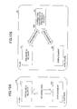
- FIG. 1 is a diagram for explaining a numerical simulation using the IT type ALE method.
- An algorithm or program according to the ALE method is executed by a computer system 1 illustrated in FIG. 1 .
- the computer system 1 includes an input device 2, a computer 3 (or a processor) 3, and an output device 4.
- the input device 2 inputs to the computer 3 information including physical constants of the fluid and structure (for example, viscosity coefficient, density, Young's modulus, etc.) and initial condition, computing region (or domain), and mesh information.
- the output device 4 outputs information computed in the computer 3, including numerical information on the degree of freedom of the fluid pressure at each discrete time step, changes in the velocity or structure, visualization information, and the like.
- the algorithm or program according to the ALE method includes a mesh information read part 6 to read mesh information from the input device 2, a graph information forming part 7 to form graph information called connectivity among nodes of discretised computing regions (that is, a node list forming finite elements), an initial condition set part 8 to set the initial condition, and a main time development loop part 9 to repeat N time steps.
- FIG. 2 is a diagram for explaining an example of the structure of the main time development loop part 9 according to the IT type ALE method.
- the main time development loop part 9 includes a FSI part 11 and a mesh control part 12.
- the FSI part 11 forms the unit that simulates physical phenomena.
- the FSI part 11 includes a matrix creating routine 111 to create a small matrix and an equivalent nodal force of each element of the structure in correspondence with the time discretization technique, a matrix creating routine 112 to create a small matrix and an equivalent nodal force of each element of the fluid in correspondence with the time discretization technique, and a boundary condition applying routine 113 to apply the boundary condition of the structure and the fluid.
- the FSI part 11 further includes a matrix assembler routine 114 to create a matrix equation with respect to all degrees of freedom by restructuring the contribution from the small matrices of each element obtained from the routines 111 through 113, a linear solver 115 to solve and evaluate a variation of dependent variables (pressure, velocity, displacement, etc.) of the fluid and the structure every time a Newton-Raphson loop within the FSI part 11 is executed, and an output part 116 to output, by displaying, for example, the variation of the dependent variables and the evaluation thereof obtained by the linear solver 115.
- a matrix assembler routine 114 to create a matrix equation with respect to all degrees of freedom by restructuring the contribution from the small matrices of each element obtained from the routines 111 through 113
- a linear solver 115 to solve and evaluate a variation of dependent variables (pressure, velocity, displacement, etc.) of the fluid and the structure every time a Newton-Raphson loop within the FSI part 11 is executed
- the mesh control part 12 within the main time development loop 9 has the role of recovering from mesh mismatch (or mesh inconsistency) caused by the node mismatch, and forms an auxiliary part to enable the numerical solving. More particularly, the mesh control part 12 recovers from the mesh mismatch state to the mesh matched state by using the displacement of the structure as the boundary condition and treating the mesh of the fluid region as an elastic body.
- the mesh control part 12 includes a matrix creating routine 121 to create the small matrix for each element of the structure, a boundary condition applying routine 122 to apply the boundary condition of the displacement of the structure, a matrix assembler routine 124 to create the matrix equation with respect to all degrees of freedom, and a solver 125 to evaluate the state of the mesh matching (or consistency of the meshes, hereinafter referred to as "mesh consistency") every time a loop is executed within the mesh control part 12.
- the target of the mesh control simulation is treated as a non-linear elastic body, the loop of Newton-Raphson method is executed iteratively in the mesh control part 12. In contrast, if the target of the mesh control simulation can be treated as a linear elastic body, the process escapes from the loop when the Newton-Raphson loop is executed once within the mesh control part 12.
- the mesh control part 11 must carry out the mesh control described above, however, the mesh control has a possibility of failing particularly in a large-displacement problem.
- the mesh control fails, the execution of the simulation stops, and an approximate solution to be obtained may not be obtained.
- the meshes will definitely fail (because a fluid mesh having zero volume is generated by the contact), and the application of the mesh control is limited.
- the amount of computations to be executed by the mesh control part 11 is relatively large, a load of the computations on the mesh control part 11 (that is, the computer 3) is relatively large.
- the conventional fluid structure interaction simulation method using the IT type ALE method is dependent on the mesh consistency between the fluid and the structure, and may not treat the large-deformation problem and the problem in which the structures contact each other. Furthermore, the load of the computations on the computer is relatively large because of the relatively large amount of computations required by the mesh control.
- the pressure and the velocity gradient change discontinuously before and after the boundary surface (for example, a thin film structure) of the fluid and the structure, and the flow may not be approximated accurately by the basis function of the general finite element method if the mesh mismatch occurs between the fluid and the structure. This is because the basis function of the finite element method is usually defined so that the pressure and the velocity gradient within the element become continuous functions, and the discontinuity within the element may not be represented.
- this proposed method does not perform the simulation with a realistic Reynolds number.
- this proposed method may generate an unnatural back flow (or reflux) before and after the structure due to the effects of the constraint condition.
- the conventional fluid structure interaction simulation method using the IT type ALE method depends on the mesh consistency between the fluid and the structure, and the load of the computations on the computer is relatively large due to the relatively large amount of computations required for the mesh control.
- the IC (Interface-Capturing) type conventional fluid structure interaction simulation method that does not depend on the mesh consistency, it may be difficult to perform an accurate simulation.
- the conventional fluid structure interaction simulation methods suffer from a problem in that it may be difficult to perform an accurate simulation without being dependent on the mesh consistency between the fluid and the structure.
- a fluid structure interaction simulation method to be implemented in a computer, that includes a graph information forming process, executed by the computer, to form graph information of nodes obtained by discretising a computing region for each of a fluid and a structure that are represented by meshes, and a main time development loop process, executed by the computer, to simulate a physical phenomenon
- the main time development loop process includes arranging interaction mediating elements that move with a displacement of the structure, on a boundary of the structure, defining, within the interaction mediating element, correcting functions of a pressure and a velocity of the fluid that interact with the pressure and the velocity of the fluid and the displacement of the structure, and executing a simulation based on the correcting functions, in a state in which the meshes of the fluid are mismatched to the meshes of the structure.
- a fluid structure interaction simulation apparatus including a storage part configured to store a program, and a processor configured to perform a fluid structure interaction simulation by executing the program, wherein the processor includes a graph information forming part configured to form graph information of nodes obtained by discretising a computing region for each of a fluid and a structure that are represented by meshes, and a main time development loop part configured to simulate a physical phenomenon, wherein the main time development loop part performs a process including arranging interaction mediating elements that move with a displacement of the structure, on a boundary of the structure, defining, within the interaction mediating element, correcting functions of a pressure and a velocity of the fluid that interact with the pressure and the velocity of the fluid and the displacement of the structure, and executing a simulation based on the correcting functions, in a state in which the meshes of the fluid are mismatched to the meshes of the structure.
- a non-transitory computer-readable storage medium that stores a program which, when executed by a computer, causes the computer to perform a fluid structure interaction simulation process including a graph information forming process, executed by the computer, to form graph information of nodes obtained by discretising a computing region for each of a fluid and a structure that are represented by meshes, and a main time development loop process, executed by the computer, to simulate a physical phenomenon
- the main time development loop process includes arranging interaction mediating elements that move with a displacement of the structure, on a boundary of the structure, defining, within the interaction mediating element, correcting functions of a pressure and a velocity of the fluid that interact with the pressure and the velocity of the fluid and the displacement of the structure, and executing the simulation based on the correcting functions, in a state in which the meshes of the fluid are mismatched to the meshes of the structure.
- graph information among nodes of discretised computing regions is formed for each of a fluid and a structure represented by meshes, in order to execute a main time development loop that simulates a physical phenomenon.
- the main time development loop arranges an IME that moves according to a displacement of the structure, on a boundary of the structure.
- the main time development loop defines correcting functions of a pressure and a velocity of the fluid, which interact with the velocity of the fluid and the displacement of the structure, in order to cause the correcting functions to bear the interaction of the fluid and the structure.
- a simulation is executed in a mesh mismatch state between the fluid and the structure.
- FIG. 3 is a block diagram illustrating an example of a fluid structure interaction simulation apparatus in an embodiment of the present invention.
- the fluid structure interaction simulation apparatus is formed by a computer system.
- a computer system 20 includes a CPU (Central Processing Unit) 21, a network interface (I/F) 22, a storage unit 23, an input device 24 including a keyboard, a mouse, and the like, and a display device 25 that are connected via a bus 26.
- the CPU 21 controls the entire computer system 20, and executes a fluid structure interaction simulation program in order to realize a fluid structure interaction simulation function.
- the I/F 22 includes a function to output commands (or requests) and data sent from the computer system 20 to a network (not illustrated), and to input commands and data received from the network to the computer system 20.
- the storage unit 23 stores various programs including the fluid structure interaction simulation program to be executed by the CPU 21, mesh information of a fluid and a structure represented by meshes, and various data including intermediate data of computations (or operations) executed by the CPU 21.
- the input device 24 is used by a user to input various commands and data to the CPU 21.
- the display device 25 displays screens (or menus) urging an operation to be performed by the user, results of simulations and evaluations executed by the CPU 21, and the like.
- the storage unit 23 may be formed by any suitable non-transitory (or tangible) computer-readable storage medium.
- the computer-readable storage medium may include magnetic recording media, optical recording media, magnetooptical recording media, disk drives using recording media in the form of disks, and semiconductor memory devices such as a ROM (Read Only Memory).
- a relation satisfying a viscous operator of a Newtonian Fluid based on Green's theorem of the following formula (1) is regarded as a limiting condition, and the method of Lagrangian multipliers are used, in order to introduce to the analysis a viscous condition at a boundary surface due to viscosity.
- v denotes an outward pointing normal unit vector defined on boundaries ⁇ of a control volume ⁇ .
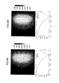
- FIGS. 4A and 4B are diagrams illustrating numerical solutions to a steady problem (Poisson's equation), that is, the equation (2) and (3) and the condition (5), for a case in which meshes conforming to the curved surface ⁇ are used and a case in which an analysis of the embodiment is used respectively.
- Poisson's equation a steady problem
- FIG. 4A illustrates, for comparison purposes, the analysis result for the case in which the meshes conforming to the curved surface ⁇ are used
- FIG. 4B illustrates the analysis result of the embodiment.
- an upper portion illustrates the numerical solutions by contour lines (level set) in the neighborhood of the curved surface ⁇ at a central cross section along a depth direction of the domain
- the ordinate in the graph of the lower portion in each of FIGS. 4A and 4B indicates a solution v
- the abscissa indicates a spatial coordinate x.
- a computing condition is represented by the following.
- g x - 1.0 ⁇ 10 - 3
- V x ⁇ y ⁇ z 1.2 - 0.3 ⁇ x x ⁇ ⁇ ⁇
- a corresponding weak form (14) can be represented as follows.
- Equation (14) p denotes the density of the fluid, and ⁇ denotes the viscosity coefficient of the fluid.
- the velocity of the fluid is denoted by v: ⁇ R 3 ⁇ R 3
- the formula satisfied by the viscous operator corresponding to the formula (1), obtained from the Green's theorem can be represented as following equation (15).
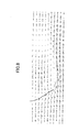
- FIGS. 5A and 5B are diagrams illustrating numerical solutions to a steady problem (viscous operator) for the case in which meshes conforming to the curved surface ⁇ are used and the case in which the analysis of the embodiment is used respectively.
- FIG. 5A illustrates, for comparison purposes, the analysis result for the case in which the meshes conforming to the curved surface ⁇ are used
- FIG. 5B illustrates the analysis result of the embodiment.
- a left portion illustrates the velocity at a central cross section along a depth direction of the domain
- the ordinate in the graph of the right portion in each of FIGS. 5A and 5B indicates a spatial coordinate in a direction perpendicular to the curved surface ⁇
- the abscissa indicates a x-component of a dependent variable v.
- the numerical solutions illustrated in FIG. 5B are affected by the boundary condition of the curved surface ⁇ in a slightly wider range in the neighborhood of the curved surface ⁇ . However, it was confirmed that the numerical solutions illustrated in FIG. 5B also reproduce the bend in the solutions on the curved surface ⁇ and approximately matches the solutions illustrated in FIG. 5A .
- the weak form can be represented by the following formula (24) by representing a boundary where a stress ⁇ is applied by ⁇ .
- ⁇ s ⁇ d 2 ⁇ d d ⁇ t 2 ⁇ X ⁇ S ⁇ F T + ⁇ s ⁇ f
- the constraint condition of the incompressibility condition that realizes the discontinuity of the pressure as proposed in Hisada et al. may be used, for example.
- the following formula (29) stands, using an arbitrary continuously differentiable function other than ⁇ , whose support is the range of a spatial scale ⁇ from the curved surface ⁇ .
- the continuously differentiable function have a value 0 at the support boundary other than ⁇ , vary its value discontinuously before and after ⁇ as in the case of a function p ⁇ illustrated in FIG. 10A .
- ⁇ ⁇ ⁇ ⁇ p ⁇ ⁇ ⁇ d ⁇ x - ⁇ ⁇ ⁇ ⁇ p ⁇ ⁇ ⁇ d ⁇ x + ⁇ ⁇ ⁇ p ⁇ ⁇ ⁇ ⁇ ⁇ d ⁇ s
- the viscous boundary condition (27) is applied to the weak form of the incompressibility condition in order to obtain the following constraint condition (30).
- ⁇ ⁇ ⁇ ⁇ p ⁇ ⁇ ⁇ d ⁇ x ⁇ ⁇ ⁇ p ⁇ ⁇ d . ⁇ ⁇ d ⁇ s .
- J p : ⁇ ⁇ ⁇ ⁇ p ⁇ ⁇ ⁇ d ⁇ x - ⁇ ⁇ ⁇ p ⁇ ⁇ d . ⁇ ⁇ d ⁇ s .
- J p : ⁇ ⁇ ⁇ ⁇ ⁇ p ⁇ ⁇ ⁇ d ⁇ x - ⁇ ⁇ ⁇ ⁇ p ⁇ ⁇ d . ⁇ ⁇ d s + ⁇ ⁇ ⁇ ⁇ p ⁇ ⁇ ⁇ d ⁇ x - ⁇ ⁇ ⁇ p ⁇ ⁇ ⁇ d . ⁇ ⁇ d s .
- FIG. 6 is a diagram illustrating an example of a FSI simulation result (numerical solution v) using the ALE method with respect to the above described problem.
- FIG. 7 is a diagram illustrating an example of a FSI simulation result (numerical solution v) in the embodiment.
- FIG. 8 is a diagram illustrating, for comparison purposes, an example of a simulation result (numerical solution v) for a case in which only the constraint condition (30) based on the incompressibility condition of Hisada et al. is applied.
- FIGS. 6 through 8 illustrate snap-shots observed at a time when the displacement of the curved surface ⁇ becomes constant, and indicate the velocity at the central cross section along the depth direction of the domain. The plotting condition is the same for each of FIGS. 6 through 8 .
- the simulation result illustrated in FIG. 7 has a small velocity in the tangential direction in the neighborhood of the surface of the curved surface ⁇ , and it was confirmed that the viscous condition of the viscosity is satisfied.
- the velocity at the wake of the curved surface ⁇ is relatively strong, but it was confirmed that the direction of the flow and the displacement of the curved surface ⁇ approach those of the simulation result illustrated in FIG. 6 and that an improvement is observed when compared to the simulation result illustrated in FIG. 8 .
- FIG. 9 is a diagram illustrating time variations of the x-component of the displacement d at the center of the lower end of the curved surface ⁇ in respective simulations for cases in which the ALE method is applied, the embodiment is applied, and only the constraint condition (30) based on the incompressibility condition of Hisada et al. is applied.
- the ordinate indicates the x-component of the displacement d
- the abscissa indicates the time t.
- I A indicates the displacement for the case in which the ALE method is applied
- I B indicates the displacement for the case in which the embodiment is applied
- I C indicates the displacement for the case in which only the constraint condition (30) based on the incompressibility condition is applied.
- the finite element of the fluid may be discretised using hexa elements or tetra elements having bubble nodes of the velocity.
- the thin film may use a DKT (Discrete Kirchhoff Triangular) shell elements.
- the node of Lagrangian multipliers of the pressure and the velocity are arranged at the centers of the shell elements.
- the nodes of ⁇ is arranged on both top and bottom surfaces of the curved surface ⁇ , in order to realize the viscous condition for each of the top and bottom surfaces.
- the scale (or element size) of the support of the basis function of the Lagrangian multipliers may be approximately the same as the scale of the shell size.
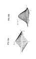
- FIGS. 10A and 10B are diagrams for explaining the basis function of the pressure and the velocity in the embodiment.
- FIG. 10A illustrates a basis function ⁇ of the pressure
- FIG. 10B illustrates a basis function ⁇ of the velocity.
- the following formulas (36) and (37) are used for the interpolation.
- the fluid structure interaction simulation that does not depend on the mesh consistency is performed based on the relation that applies the Green's theorem with respect to the viscous operator of the Newtonian fluid.
- a comparison study was made between this embodiment and the generally used IT type ALE method, with respect to the interaction of the thin film structure using the shell elements.
- the use of this embodiment safisfies the viscous condition at the structure boundary, and that the flow and the displacement of the structure reproducible by this embodiment are closer to those of the simulation result of the ALE method than the conventional techniques.
- this embodiment may suppress the back flow of the fluid that may otherwise be generated depending on the viscous condition.
- this embodiment performs the IC (Interface-Capturing) type numerical simulation with respect to the interaction of the fluid and the structure.
- Such an interaction may include the interaction of the structure that may be treated as a thin film, such as a baloon, a soap film, a fabric divider, and a flag, and the surrounding fluid, and the interaction of the structure that may be treated as a rigid body, an elastic body having a thickness such as a heart muscle, and the fluid on the inner side or the outer side of the structure.
- the finite elements of structures, such as a ribbon and a beam, that may not be defined by a two-dimensional surface, are not simulation targets of this embodiment.
- the fluid structure interaction simulation method of this embodiment may include the following procedures (or steps) ST1 through ST3.
- Procedure ST1 The interaction boundary of the fluid region and the structure becomes a moving boundary (or free boundary), and the finite element that follows the displacement of the structure in motion and moves is defined on the top and bottom surfaces of this moving boundary.
- the correcting functions of the pressure and the velocity of the fluid, having a non-zero value only within the finite element, are defined.
- Procedure ST2 In order for the defined correcting functions to be able to represent the discontinuity of the pressure and the velocity gradient while mediating the interaction of the fluid and the structure, conditions are applied to a region having a value, that is support of correcting functions, and values of functions and derived functions on the structure or the element boundary, and the like.
- Procedure ST3 In order to represent the interaction of the fluid and the structure, a weak form in which a boundary integral on the structure explicitly appears is used. This weak form is different from the weak form used in the conventional fluid structure interaction simulation. This weak form used in this procedure is based on the Green's theorem, and is derived from the incompressibility condition of fluid and the relation satisfied by the viscous operator of the fluid.
- the finite element that follows the displacement of the structure in motion and moves is defined.
- the correcting functions capable of representing the viscous condition at the boundary of the fluid and the structure and the discontinuity of the pressure and the velocity gradient at the top and bottom surfaces of the structure is introduced, while satisfying the incompressibility and the continuity of the velocity, in order to mediate the interaction of the displacement d of the structure, and the pressure p and the velocity v of the fluid.
- the finite element that is defined in this manner will be referred to as an IME (Interaction Mediating Element).
- the constraint condition based on the Green's theorem is introduced, in order to represent the correcting functions described above and the interaction of the fluid and the structure.
- the constraint condition makes it possible to realize the interaction of the fluid and the structure mediated by the correcting functions.
- this embodiment defines the weak form and the weak solution.
- the Green's theorem generalizes the integration by part, and may be represented in the following manner, where v denotes the outward pointing unit normal vector of the control volume.
- ⁇ ⁇ ⁇ u ⁇ ⁇ ⁇ ⁇ x ⁇ d ⁇ x - ⁇ ⁇ ⁇ ⁇ u ⁇ x ⁇ ⁇ d ⁇ x + ⁇ ⁇ ⁇ ⁇ u ⁇ d ⁇ s .
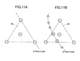
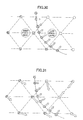
- FIGS. 11A and 11B are diagrams for explaining an independence of the degree of freedom of each finite element for a two-dimensional triangular element.
- each node is indicated by a circular symbol
- for each element of a fluid mesh 29, only the node having the interaction is indicated by a double circular symbol
- the node of the structure not shared with the fluid is indicated by a circular symbol with hatchings.
- FIG. 11A illustrates the case in which the ALE method is applied
- FIG. 11B illustrates the case in which the embodiment is applied.
- the edge of the triangular element forming the fluid part and the edge of the element match, and the nodes on the edge are shared by the two elements.
- the interaction is closed between the degrees of freedom in units of the triangular elements.
- the meshes of the fluid and the structure must constantly be matched to achieve mesh consistency in the case in which the ALE method is applied.
- the structure exists independently of the triangular element forming the fluid part.
- a set of the nodes having the interaction between the fluid and the structure changes for each time step (or discrete time) depending on the displacement of the structure, because of the independence of the degrees of freedom of each of the finite elements (that is, because of the non-dependence on the mesh consistency).
- a search may be made with respect to a part where the fluid and the structure overlap, in order to determine the set of the nodes having the interaction between the fluid and the structure.
- the elements may be defined as the set of nodes having such an interaction. Accordingly, in the case in which the embodiment is applied, the simulation may be performed in the mesh mismatch state in which the meshes of the fluid and the structure do not match.
- the IME that mediates the interaction between the fluid and the structure arranged on the structure surface, enables the simulation to be executed in the mesh mismatch state.
- the constraint condition dependent on the incompressibility and the relation satisfying the viscous operator of the fluid are used for the interaction of the fluid and the structure, based on the Green's theorem.
- FIGS. 12A and 12B are diagrams for explaining a fluid and structure interaction.
- FIG. 12A illustrates the interaction of the fluid and the structure using the ALE method
- FIG. 12B illustrates the interaction of the fluid and the structure using the embodiment.
- the set of interacting nodes are closed (that is, finite elements) for each of small regions segmenting (or discretising) respective regions of a fluid 311 and a structure 312 is a non-overlapping manner, and the degrees of freedom of the nodes interact.
- the degree of freedom of the node is, for example, the pressure p and the velocity v in the case of the fluid 311, and is the displacement d or the like in the case of the structure 312.
- an IME 33 that mediates the interaction is defined on the structure 32 in motion, and the correcting functions are defined within the IME 33 for the pressure and the velocity of the fluid 31.
- the IME 33 that is a finite element moving in accordance with the displacement of the structure 32, is arranged on the boundary of the structure 32, and the correcting functions with respect to the pressure and the velocity of the fluid 31 are defined within the IME 33.
- the correcting functions are Lagrangian multipliers, as the limiting condition, whose constraints are the incompressibility condition of the fluid 31 in the neighborhood of the boundary of the fluid 31 and the structure 32 and the relation satisfied by the viscous operator of the Newtonian fluid, based on the Green' theorem. Because the IME 33 moves by following the displacement of the structure 32, an interaction pair formed by the IME 33 and the degree of freedom of the structure 32 does not change, but an interaction pair of the IME 33 and the degree of freedom of the fluid 31 changes as the IME 33 moves every moment. Hence, a background fluid element that overlaps the IME 33 is searched, in order to determine the interaction pair with the IME 33 from the fluid node that is a member of the fluid element.
- the IC type numerical simulation that is, the fluid structure interaction simulation, can be executed based on the interaction pair that is determined in this manner.
- Each degree of freedom of the fluid 31 may recognize the interaction boundary with the structure 32 in motion through the IME 33, and an appropriate interaction may be obtained, to thereby eliminate the dependence on the mesh consistency of the meshes of the fluid 31 and the structure 32.
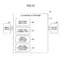
- FIG. 13 is a diagram for explaining an IC type numerical simulation in the embodiment.
- the algorithm or the program of the IC type numerical simulation is executed by a computer system 41 illustrated in FIG. 13 .
- the computer system 41 includes an input device 42, a computer 43, and an output device 44.
- the input device 42 may be formed by at least one of the input device 24 and the I/F 22 illustrated in FIG. 3 , for example.
- the input device 42 inputs the physical constants (for example, the viscosity and density, Young's modulus, etc.) of the fluid and the structure and the initial condition, the computing region (or domain) and the mesh information to the computer 43.
- the output device 44 may be formed by the display device 25 illustrated in FIG. 3 , for example.
- the output device 44 may output, as the simulation result, the numerical information of the degrees of freedom of the pressure and the velocity of the fluid and the displacement of the structure computed by the computer 43 at each discrete time step, the visualization information, and the like.
- This embodiment unlike the case in which the ALE method is used, creates the graph (or connectivity) of the meshes for both the fluid and the structure, and separately creates the graph for the two-dimensional element forming the interaction boundary of the fluid and the structure when creating the graph of the meshes if the structure has a three-dimensional distribution.
- the structure has the three-dimensional structure when the element has a volume, that is, when the element does not relate to a two-dimensional "surface" such as the shell and the film element.
- the IC type numerical simulation algorithm or program includes a mesh information read part 46 to execute a mesh information read process that reads the mesh information from the input device 42, a graph information forming part 47 to execute a graph information forming process that forms the graph information called the connectivity among nodes of discretised computing regions (that is, a node list forming finite elements) for both the fluid and the structure, an initial condition set part 48 to execute an initial condition setting process that sets the initial condition, and a main time development loop part 49 to execute a main time development loop process that repeats the N time steps.
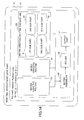
- FIG. 14 is a diagram for explaining an example of a structure of the main time development loop part of the IC type embodiment.
- the main time development loop part 49 includes a FSI part 51.
- the FSI part 51 simulates the physical phenomena.
- the FSI part 51 includes a matrix creating routine 151 to create a small matrix and an equivalent nodal force for each element of the structure in correspondence with the time discretization technique, a matrix creating routine 152 to create a small matrix and an equivalent nodal force for each element of the fluid in correspondence with the time discretization technique, a matrix creating routine 153 to create a matrix representing the interaction of the velocity, pressure, and the correcting functions for each IME, a matrix assembler routine 155 to create a matrix equation with respect to all degrees of freedom by restructuring the contribution from the small matrices for each element obtained from the routines 151, 152, and 153, a linear solver 156 to solve and evaluate a variation of dependent variables (pressure, velocity, displacement, etc.) of the fluid and the
- a boundary condition applying part within the matrix creating part 153 includes modules 61 through 64 representing the interaction of the correcting functions and the displacement of the structure.
- the IME that moves by following the displacement of the structure in motion is generated by the modules 61 through 64, and the isolation of the meshes of the fluid and the structure (that is, the non-dependence on the mesh consistency) is realized.
- the modules 61 through 64 will be referred to as sub parts 61 through 64 for the sake of convenience.
- the first sub part 61 computes an interaction matrix of the correcting function of the pressure and the velocity of the fluid.
- the second sub part 62 computes an interaction matrix of the correcting function of the velocity and the velocity of the fluid.
- the third sub part 63 computes an interaction matrix of the correcting function of the pressure and the displacement velocity of the structure.
- the fourth sub part 64 computes an interaction matrix of the correcting function of the pressure and the displacement velocity of the structure.
- FIG. 15 is a diagram illustrating an example of a composition of the first sub part 61.
- the size (or spatial scale) ⁇ , the graph (or connectivity) of each of the meshes in the fluid region and the structure region that is created in advance, and the node coordinate are input to the first sub part 61.
- the first sub part 61 includes a search part 611, an allocation part 612, and a fluid contribution computing part 613.
- the search part 611 searches for a set of fluid nodes that are interacted upon by the finite element that moves by following the displacement of the structure, which finite element is defined for each two-dimensional element forming the interaction boundary ⁇ of the fluid and the structure.
- the allocation part 612 allocates a memory region that is required based on a search result of the search part 611.
- the fluid contribution computing part 613 computes the contribution of the matrix to the degree of freedom of each node.
- the displacement of the structure is determined independently of the meshes of the fluid, and the list of fluid nodes that are interacted upon by the IME differs every time the time development and the Newton-Raphson loop is executed.
- the search is performed to update the list of interacting nodes.
- the search part 611 uses the cell index method (or bucket sorting method) to perform the search.
- the cell index method segments (or discretises) the domain ⁇ into rectangular cells, and all elements are made to correspond to the cells according to the coordinate of the center of volume, in order to perform the search in units of cells.
- the search part 611 determines the number of fluid nodes to which each IME interacts.
- the fluid element to be included is searched using the cell index method for each of the integral points, and the number of velocity nodes that are constituent members of the fluid element is counted.
- the integration is performed using the Gaussian quadrature for each of the fluid elements defined in the global domain
- a confirmation is made to determine whether the IME includes the integral points of the Gaussian quadrature of the fluid elements included in peripheral cells surrounding a central cell that includes the center of volume of the IME, and the number of velocity nodes that are constituent members of the fluid element is counted if the IME includes the integral points of the Gaussian quadrature of the fluid elements included in the peripheral cells.
- the search part 611 executes procedures (or processes) of (s1) obtaining the integral point coordinate within the IME moving together with the interaction boundary, (s2) searching the fluid element including the integral points, and (s3) counting the fluid nodes (or the degrees of freedom) that are members of the searched fluid element as the interaction nodes without overlap, based on the graph information of the meshes.
- the search part 611 executes procedures (or processes) of (s1') obtaining the coordinate of the center of volume of the IME moving together with the interaction boundary, (s2') searching the fluid element surrounding the center of volume from the center of volume, and (s3') counting the fluid nodes (or the degrees of freedom) that are members of the searched fluid element as the interaction nodes without overlap, if the IME includes the Gaussian quadrature points of the fluid element.
- the allocation part 612 allocates the memory region to store the contribution to the matrix, based on the number of interaction nodes counted in the search part 611.
- the fluid contribution computing part 613 performs a process similar to that performed by the search part 611, in order to create a list of the interacting fluid nodes for each IME, and simultaneously computes the contribution to the interaction matrix. Accordingly, in a case in which the integration is performed using the integral points discretely arranged within the IME, the search part 611, with respect to each IME defined for each of the two-dimensional elements forming the interaction boundary ⁇ , executes procedures (or processes) of (s11) obtaining the integral point coordinate within the IME moving together with the interaction boundary, (s12) searching the fluid element including the integral points, (s13) storing the fluid nodes (or the degrees of freedom) that are members of the searched fluid element in the memory based on the graph information of the meshes, (s14) obtaining the basis function value and the derived function at the integral points, and (s15) adding the contributions to the small matrix within the element.
- the fluid contribution computing part 613 executes procedures (or processes) of (s11') obtaining the coordinate of the center of volume of the IME moving together with the interaction boundary, (s12') searching the fluid element surrounding the center of volume from the center of volume, (s13') storing the fluid nodes (or the degrees of freedom) that are members of the searched fluid element in the memory based on the graph information of the meshes, if the IME includes the Gaussian quadrature points of the fluid element, (S14') obtaining the basis function value and the derived function at the integral points, and (s15') adding the contributions to the small matrix within the element.
- each of the memories described hereunder may be formed by the storage unit 23 illustrated in FIG. 3 , for example. Hence, it is possible to create the small matrix for each element, representing the interaction of the correcting function of the pressure and the velocity of the fluid defined in the global domain.
- FIG. 16 is a flow chart for explaining the operation of first and second sub parts.
- FIG. 17 is a diagram for explaining a process A illustrated in FIG. 16
- FIG. 18 is a diagram for explaining a process B illustrated in FIG. 16.
- FIG. 16 illustrates the process for an example in which the integration is performed using the integral points discretely arranged within the IME.
- the processes A and B are not performed by the procedures (s1) through (s3) described above, and the processes A and B are performed by the procedures (s11) through (s15) described above.
- the process A is performed only when a flag "ndflag” and a flag “matime” are allocated.
- the flags "ndflag” and “matime” are allocated when integrating the integral points discretely arranged within the IME.
- a step S12 searches for a fluid element "jelem” that includes the integral point coordinate "tpoint”, using the cell index method.
- a step S13 initializes a node ID "jnode” within the fluid element "jelem” to "0".
- a step S161 in FIG. 18 obtains the basis function at the integral point and the gradient of the basis function in the fluid element "jelem".
- a step S162 obtains the basis function at the integral point and the gradient of the basis function in the IME.
- a step S163 multiples the weight at the integral point to the basis function and its gradient, and evaluates a contribution "contrib.” of the integral term in the weak form.
- the process returns to the step S14 if the decision result in the step S17 is FALSE, and the process advances to a step S18 if the decision result in the step S17 is TRUE.
- the process returns to the step S10 if the decision result in the step S18 is FALSE, and the process advances to a step S19 if the decision result in the step S18 is TRUE.
- the process returns to the step S7 if the decision result in the step S19 is FALSE, and the process advances to a step S20 if the decision result in the step S19 is TRUE.
- FIG. 19 is a diagram illustrating an example of a structure of the second sub part 62.
- the input to the second sub part 62 is the same as the input to the first sub part 61 described above.
- the second sub part 62 includes a search part 621, an allocation part 622, and a fluid contribution computing part 623.
- the search part 621 searches for a set of fluid nodes that are interacted upon by the finite element that moves by following the displacement of the structure, which finite element is defined on the top surface and the bottom surface of the structure for each two-dimensional element forming the interaction boundary ⁇ of the fluid and the structure.
- the allocation part 622 allocates a memory region that is required based on a search result of the search part 621.
- the fluid contribution computing part 623 computes the contribution of the matrix to the degree of freedom of each node.
- the displacement of the structure is determined independently of the meshes of the fluid, and the list of fluid nodes that are interacted upon by the IME differs every time the time development and the Newton-Raphson loop is executed.
- the search is performed to update the list of interacting nodes.
- the search part 621 uses the cell index method to perform the search.
- the search part 621 determines the number of fluid nodes to which each IME interacts. More particularly, in the case in which the integration is performed using the integral points arranged discretely within the IME, the fluid element to be included is searched using the cell index method for each of the integral points, and the number of velocity nodes that are constituent members of the fluid element is counted.
- a confirmation is made to determine whether the IME includes the integral points of the Gaussian quadrature of the fluid elements included in peripheral cells surrounding a central cell that includes the center of volume of the IME, and the number of velocity nodes that are constituent members of the fluid element is counted if the IME includes the integral points of the Gaussian quadrature of the fluid elements included in the peripheral cells.
- the search part 621 executes procedures (or processes) of (s21) obtaining the integral point coordinate within the IME moving together with the interaction boundary, (s22) searching the fluid element including the integral points, and (s23) counting the fluid nodes (or the degrees of freedom) that are members of the searched fluid element as the interaction nodes without overlap, based on the graph information of the meshes.
- the search part 621 executes procedures (or processes) of (s21') obtaining the coordinate of the center of volume of the IME moving together with the interaction boundary, (s22') searching the fluid element surrounding the center of volume from the center of volume, and (s23') counting the fluid nodes (or the degrees of freedom) that are members of the searched fluid element as the interaction nodes without overlap, if the IME includes the Gaussian quadrature points of the fluid element.
- the allocation part 622 allocates the memory region to store the contribution to the matrix, based on the number of interaction nodes counted in the search part 621.
- the fluid contribution computing part 623 performs a process similar to that performed by the search part 621, in order to create a list of the interacting fluid nodes for each IME, and simultaneously computes the contribution to the interaction matrix. Accordingly, in a case in which the integration is performed using the integral points discretely arranged within the IME, the search part 611, with respect to each IME defined on the top surface and the bottom surface of the interaction boundary ⁇ for each of the two-dimensional elements forming the interaction boundary ⁇ , executes procedures (or processes) of (s31) obtaining the integral point coordinate within the IME moving together with the interaction boundary, (s32) searching the fluid element including the integral points, (s33) storing the fluid nodes (or the degrees of freedom) that are members of the searched fluid element in the memory based on the graph information of the meshes, (s34) obtaining the basis function value and the derived function at the integral points, and (s35) adding the contributions to the small matrix within the element.
- the fluid contribution computing part 623 executes procedures (or processes) of (s31') obtaining the coordinate of the center of volume of the IME moving together with the interaction boundary, (s32') searching the fluid element surrounding the center of volume from the center of volume, (s33') storing the fluid nodes (or the degrees of freedom) that are members of the searched fluid element in the memory based on the graph information of the meshes, if the IME includes the Gaussian quadrature points of the fluid element, (S34') obtaining the basis function value and the derived function at the integral points, and (s35') adding the contributions to the small matrix within the element.
- the process of the second sub part 62 may be performed in a manner similar to the process of the first sub part 61 described above in conjunction with FIG. 16 .
- the processes A and B are not performed by the procedures (s21) through (s23), and the processes A and B are performed by the procedures (s31) through (s35).
- the process of the step S101 in the process A for the second sub part 62 partially differs from that for the first sub part 61.
- the small matrix is created for each element representing the interaction of the correcting function of the velocity and the velocity of the fluid defined in the global domain.
- FIG. 20 is a diagram illustrating an example of a structure of the third sub part 63.
- the input to the third sub part 63 is the same as the input to the first sub part 61 described above.
- the third sub part 63 regards that the structure elements interacting with each element solely include the structure elements on which the elements are arranged, and does not perform a search.
- the third sub part 63 includes an allocation part 631 to allocate a memory region that is required, and a structure contribution computing part 632 to compute the contribution of the matrix to the degree of freedom of each node.
- the structure contribution computing part 632 computes the boundary integral term on the interaction boundary ⁇ , that is obtained using the Green's theorem in order to represent the interaction of the correcting function of the pressure and the interaction of the velocity of the structure.
- the allocation part 631 regards that displacement nodes of the interacting structure solely include nodes of the structure element arranged with the IME, and allocates the memory region that is required to store the contribution to the matrix, for each IME.
- the structure contribution computing part 632 computes the contribution to the interacting matrix, by regarding the displacement nodes of the structure element arranged with each IME as the interacting nodes. More particularly, with respect to each IME defined for each of the two-dimensional elements forming the interaction boundary ⁇ , the structure contribution computing part 632 executes procedures (or processes) of (s41) storing the structure nodes (or the degrees of freedom) that are members of the structure element arranged with the IME and form an interaction pair in the memory, and (s42) adding the contributions to the small matrix within the element. Hence, the incompressibility condition is applied, and the small matrix is created for each element representing the interaction of the correcting function of the pressure and the velocity of the structure.
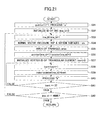
- FIG. 21 is a flow chart for explaining the operation of the third and fourth sub parts.
- FIG. 22 is a diagram for explaining a process "a" illustrated in FIG. 21
- FIG. 23 is a diagram for explaining a process "b" illustrated in FIG. 21 .
- a step S35 defines an area "area" of a triangle.
- a step S40 executes the process "b" illustrated in FIG. 23 .
- a step S401 illustrated in FIG. 23 evaluates a contribution "contrib.” of the integral term in the weak form, by focusing on the normal vector "vn” and the element area “area” .
- the process returns to the step S38 if the decision result in the step S41 is FALSE, and the process advances to a step S42 if the decision result in the step S41 is TRUE.
- the process returns to the step S33 if the decision result in the step S42 is FALSE, and the process ends if the decision result in the step S42 is TRUE.
- FIG. 24 is a diagram illustrating an example of a structure of the fourth sub part 64.
- the input to the fourth sub part 64 is the same as the input to the first sub part 61 described above.
- the fourth sub part 64 regards that the structure elements interacting with each element solely include the structure elements on which the elements are arranged, and does not perform a search.
- the fourth sub part 64 includes an allocation part 641 to allocate a memory region that is required, and a structure contribution computing part 642 to compute the contribution of the matrix to the degree of freedom of each node.
- the structure contribution computing part 642 computes the boundary integral term on the interaction boundary ⁇ , that is obtained using the Green's theorem in order to represent the interaction of the correcting function of the velocity and the interaction of the velocity of the structure.
- the allocation part 641 regards that displacement nodes of the interacting structure solely include nodes of the structure element arranged with the IME, and allocates the memory region that is required to store the contribution to the matrix, for each IME.
- the structure contribution computing part 642 computes the contribution to the interacting matrix, by regarding the displacement nodes of the structure element arranged with each IME as the interacting nodes. More particularly, with respect to each IME defined on the top surface and the bottom surface of the interaction boundary ⁇ for each of the two-dimensional elements forming the interaction boundary ⁇ , the structure contribution computing part 642 executes procedures (or processes) of (s51) storing the structure nodes (or the degrees of freedom) that are members of the structure element arranged with the IME and form an interaction pair in the memory, and (s52) adding the contributions to the small matrix within the element. Hence, the viscous condition is applied, and the small matrix is created for each element representing the interaction of the correcting function of the velocity and the velocity of the structure.
- the process of the fourth sub part 64 may be performed in a manner similar to the process of the third sub part 63 described above in conjunction with FIG. 21 . Further, as described above in conjunction with FIG. 22 , the process of the step S311 in the process "a" for the fourth sub part 64 partially differs from that for the third sub part 63.
- this embodiment uses the finite element (IME) that moves with the displacement of the structure, and is arranged on the surface (curved surface) ⁇ that becomes the interaction boundary (that is, the moving boundary or the free boundary) of the fluid region and the structure region.
- IME finite element
- the pressure correcting function having a non-zero value only within the IME and having a zero value at the element boundary other than the interaction boundary, and the velocity correcting function having a non-zero value only within the IME and having a zero gradient at the element boundary other than the interaction boundary are used.
- the weak form that is different from that of the conventional fluid and structure interaction is used to represent the interaction of the fluid and the structure.
- the interaction boundary ⁇ of the fluid and the structure, that becomes the moving boundary (or free boundary), is segmented (or discretised) two-dimensionally into elements according to the segmenting (or discretization) of the structure into the finite elements.
- the center, vertex, and integral point of the two-dimensional finite element forming the interaction boundary ⁇ may be used as representative points to arrange the node of the pressure correcting function.
- Elements having the spherical or right circular cylinder shape and a size ⁇ are arranged on the top surface and the bottom surface of the interaction boundary ⁇ , using the node as a center, in order to define the correcting function of the pressure of the fluid within the element.
- the center, vertex, and integral point of the two-dimensional finite element forming the interaction boundary ⁇ may be used as representative points to arrange the node of the velocity correcting function on the top surface and the bottom surface of the interaction boundary ⁇ .
- Elements having the spherical or right circular cylinder shape and a size ⁇ are arranged on the top surface and the bottom surface of the interaction boundary ⁇ , using the node as a center, in order to define the correcting function of the velocity of the fluid within the element.
- FIGS. 25A and 25B are diagrams illustrating an image of the IMEs that move by following the displacement of the structure that undergoes motion, and is discretely arranged on the interaction boundary ⁇ of the fluid and the structure.
- FIG. 25A illustrates the IMEs with respect to the pressure correcting function, defined to span the top surface and the bottom surface, and wherein the elements on the top surface and the bottom surface of the interaction boundary ⁇ correspond to one node.
- FIG. 25B illustrates the IMEs with respect to the velocity correcting function, and wherein the elements are similarly arranged on both the top surface and the bottom surface of the interaction boundary ⁇ .
- FIGS. 25A and 25B illustrate elements having a hemisphere shape, for example, and the elements are illustrated as having a relatively small element size for eye-friendly sake However, the element size may be determined so that IMEs mutually overlap.
- the size ⁇ of the IME that moves by following the displacement of the structure in motion may be selected such that the IMEs overlap without a gap therebetween on the interaction boundary ⁇ of the fluid and the structure.
- the support of each of the correcting functions may have a length scale of approximately ⁇ .
- the smaller the length scale ⁇ the more the performance of the Lagrangian multipliers satisfying the constraint condition improves, to thereby making the introduction of the correcting functions ideal.
- the smaller the length scale ⁇ the more difficult it becomes to improve the numerical integration accuracy.
- the pressure P of the fluid may be defined by the following formula (38) using the continuous pressure p that is globally defined and the pressure correcting function p ⁇ having the support only in the neighborhood of the interaction boundary ⁇ .
- P p + p ⁇
- the pressure correcting function p ⁇ has a positive value on one side specified by a normal n(y) (y ⁇ ) that is uniquely defined on the interaction boundary ⁇ , a negative value on the other side by undergoing discontinuous changes on the interaction boundary ⁇ , a non-zero value on the interaction boundary ⁇ , a zero value on the support boundary other than the interaction boundary ⁇ , and may be defined by the following formula (39) using a function ⁇ that is once continuously differentiable within the support but excluding the interaction boundary ⁇ .
- P ⁇ 0 denotes a function representing a pressure difference defined on the interaction boundary ⁇ .
- FIGS. 26A and 26B are diagrams for explaining the basis function ⁇ of the pressure correcting function.
- FIG. 26A illustrates the basis function ⁇ with respect to the normal v
- FIG. 26B illustrates the basis function ⁇ with respect to the normal v and the interaction boundary ⁇ .
- the basis function ⁇ has the following properties.
- the definition thereof may be made using a coordinate system that is easily treatable depending on the shape of the IME that is to be added.
- the example of the basis function is a polynomial, however, a low-order basis function may be used because of the need to increase the resolution of the numerical integration when a high-order basis function is used.
- an open hemisphere included in a half space specified by a radius ⁇ and a normal v may be represented by the following.
- B ⁇ ⁇ y : ⁇ y ⁇ ⁇
- FIG. 27 is a diagram for explaining the definition of the open hemisphere and polar coordinates.
- the right circular cylinder included in the half space specified by the radius and the height respectively denoted by ⁇ and the normal denoted by v may be represented by the following.
- FIG. 28 is a diagram for explaining the right circular cylinder and the polar coordinates.
- each basis function is non-zero and discontinuous on the interaction boundary ⁇ , and has a zero value at the support boundary other than the interaction boundary ⁇ .
- the velocity V of the fluid may be defined by the following formula using the velocity v that is defined in the global domain, and the velocity correcting function ⁇ ⁇ having the support on both the top surface and the bottom surface of the interaction boundary ⁇ .
- the velocity correcting function ⁇ ⁇ has a support only on one side specified by a normal n to the interaction boundary ⁇ , is twice continuously differentiable within the support, does not have a value in all support boundaries including the interaction boundary ⁇ , has a non-zero gradient at the interaction boundary ⁇ , and has a zero gradient at boundaries other than the interaction boundary ⁇ .
- the velocity correcting function ⁇ ⁇ may be defined using the following function ⁇ illustrated in FIGS.
- FIGS. 29A and 29B are diagrams for explaining the basis function of the velocity correcting function.
- FIG. 29A illustrates the basis function ⁇ with respect to the normal vector v
- FIG. 29B illustrates the basis function ⁇ with respect to the normal vector ⁇ and the interaction boundary ⁇ .
- the velocity basis function ⁇ may preferably be defined using a coordinate system that is easily treatable depending on the shape of the IME that is to be added.
- the example of the basis function is a polynomial, however, a low-order basis function may be used because of the need to increase the resolution of the numerical integration when a high-order basis function is used.
- the basis function defined by an open hemisphere B k + specified by a radius ⁇ may be represented by the following.
- ⁇ ⁇ y : ⁇ Ag r ⁇ ⁇ ⁇ ⁇ 1 B ⁇ + y : ⁇
- the following formulas (60) can be used, where (r, ⁇ , ⁇ ) is the polar coordinate illustrated in FIG. 27 .
- the values of m and n may be set relatively small.
- ⁇ ⁇ y : ⁇ Ag r ⁇ ⁇ ⁇ ⁇ ⁇ 1 C ⁇ + y : ⁇
- the values of m and n may be set relatively small.
- the dependent variables are the velocity v and the pressure p of the fluid, the displacement d of the structure, the velocity correcting function ⁇ , and the pressure correcting function p.
- 5 denotes a variational operator
- ⁇ X denotes a test function corresponding to an arbitrary function X, in accordance with custom of mechanics.
- the test function corresponding to each dependent variable becomes ( ⁇ v, ⁇ p, ⁇ d, ⁇ , ⁇ p ⁇ ) .
- the equation (64) represents the velocity and the pressure (v, p) of the fluid defined on the global domain and the interaction of the test function thereof, but the commonly available fluid code used in the ALE program, for example, may also be used.
- the equation (65) represents the displacement and the velocity ( d , ⁇ ) of the structure and the test function thereof, but the commonly available codes used in the ALE FSI program, for example, may also be used.
- ⁇ J p represents the interaction of the pressure correcting function and the interaction of the fluid and the structure, and may be derived from the incompressibility condition term and the pressure gradient term of the fluid, as may be seen from the following formula (66).
- ⁇ J p : ⁇ ⁇ ⁇ ⁇ ⁇ ⁇ p ⁇ ⁇ ⁇ d ⁇ x - ⁇ ⁇ ⁇ ⁇ p ⁇ ⁇ d . ⁇ ⁇ d s + ⁇ ⁇ ⁇ ⁇ p ⁇ ⁇ ⁇ ⁇ d ⁇ x - ⁇ ⁇ ⁇ p ⁇ ⁇ ⁇ d . ⁇ ⁇ d s .
- ⁇ denotes a union of the supports of the IMEs.
- the union ⁇ has a spread of a length scale ⁇ in the periphery around the interaction boundary ⁇ .
- ⁇ J v represents the interaction of the velocity correcting function and the interaction of the fluid and the structure, and may be derived from the viscous term of the fluid.
- ⁇ J ⁇ : ⁇ ⁇ ⁇ ⁇ ⁇ G ⁇ ⁇ ⁇ ⁇ + 2 ⁇ ⁇ ⁇ ⁇ ⁇ ⁇ D ⁇ ⁇ ⁇ ⁇ ⁇ d ⁇ x - ⁇ ⁇ ⁇ 2 ⁇ ⁇ ⁇ d .
- ⁇ denotes a union of the IMEs.
- the interaction of the fliud and the structure at parts other than on the interaction boundary ⁇ may be neglected.
- the fluid contribution computing part 613 of the first sub part 61 computes the matrices forming the following two terms represented by the volume integral, amongst the pressure gradient term and the incompressibility condition term ⁇ J p .
- ⁇ J p ⁇ ⁇ ⁇ ⁇ ⁇ ⁇ ⁇ p ⁇ ⁇ ⁇ d ⁇ x + ⁇ ⁇ ⁇ ⁇ p ⁇ ⁇ ⁇ d ⁇ x .
- the integration may divide ⁇ into ⁇ ⁇ depending on the top surface and the bottom surface of the interaction boundary ⁇ , and further decompose ⁇ ⁇ into the IMEs for each half of the element.
- the integration for each element may be approximated by a multiply-accumulate of the volume element and the function value of the integrand at the integral points regularly distributed within the element.
- 1 ⁇ ⁇ ⁇ may be multiplied to the integrand in order to carry out a Gaussian quadrature for each fluid element defined in the global domain.
- the fluid contribution computing part 623 of the second sub part 62 computes the matrices forming the following two terms represented by the volume integral of ⁇ J v representing the interaction of the velocity correcting function and the velocity of the fluid defined in the global domain.
- ⁇ J v va ⁇ 3 is the constraint condition with respect to the Lagrangian multipliers and need not be computed.
- Each of the remaining two terms represents the interaction of the velocity correcting function and the velocity of the fluid defined in the global domain.
- the integration may divide ⁇ into ⁇ ⁇ depending on the top surface and the bottom surface of the interaction boundary ⁇ , and further decompose ⁇ ⁇ into the IMEs for each half of the element.
- the integration for each element may be approximated by a multiply-accumulate of the volume element and the function value of the integrand at the integral points regularly distributed within the element.
- 1 ⁇ ⁇ ⁇ may be multiplied to the integrand in order to carry out a Gaussian quadrature for each fluid element defined in the global domain.
- the structure contribution computing part 632 of the third sub part 63 computes the matrices forming the following two terms represented by the surface integral, between the pressure gradient term and the incompressibility condition term ⁇ J p .
- J p s - ⁇ ⁇ ⁇ ⁇ ⁇ p ⁇ d . ⁇ ⁇ d ⁇ s - ⁇ ⁇ ⁇ p ⁇ ⁇ ⁇ ⁇ d . ⁇ ⁇ d s .
- the integration may be performed on the interaction boundary ⁇ for each two-dimensional element forming the interaction boundary ⁇ .
- an approximation may be used by assuming that ⁇ is uniform within each two-dimensional element e forming the interaction boundary ⁇ , and defining the value ⁇ e by an average value of the values at each of the nodes.
- the structure contribution computing part 642 of the fourth sub part 64 computes the matrices forming the following two terms represented by the surface integral of the interaction of the velocity correcting function and the displacement of the structure, represented by ⁇ J v , on the interaction boundary ⁇ .
- J ⁇ s - ⁇ ⁇ ⁇ 2 ⁇ ⁇ ⁇ d . ⁇ ⁇ ⁇ D ⁇ ⁇ ⁇ ⁇ d ⁇ s - ⁇ ⁇ ⁇ 2 ⁇ ⁇ ⁇ d . ⁇ D ⁇ ⁇ ⁇ ⁇ d ⁇ s .
- the integration may be performed on the interaction boundary ⁇ for each two-dimensional element forming the interaction boundary ⁇ , on the top surface and the bottom surface of the interaction boundary ⁇ .
- an approximation may be used by assuming that ⁇ is uniform within each two-dimensional element e forming the interaction boundary ⁇ , and defining the value ⁇ e by an average value of the values at each of the nodes.
- the integral of D ⁇ v , ⁇ D ⁇ v may be analytically obtained in advance, the integral may be approximated by the following using the analytically obtained result. ⁇ ⁇ ⁇ 2 ⁇ ⁇ ⁇ d . ⁇ ⁇ ⁇ D ⁇ ⁇ ⁇ ⁇ d ⁇ s ⁇ 2 ⁇ ⁇ d . c ⁇ ⁇ ⁇ ⁇ ⁇ ⁇ D ⁇ ⁇ ⁇ ⁇ d ⁇ s
- One object of the fluid structure interaction simulation of this embodiment is to make the meshes of the fluid and the structure independent.
- the total stress affecting the motion of the structure may be caused by the discontinuity in the velocity gradient or the pressure at the top surface and the bottom surface of the structure.
- the discontinuity in such physical quantities may easily be understood by considering a situation in which the fluid within two cylinders changes discontinuously on both sides of a valve that partitions the two cylinders. The discontinuity in the velocity is evident because no vacuum will be generated in a neighborhood of the valve.
- completely different fluid motions may be generated in the two cylinders partitioned by the valve, and thus, it may be understood that completely different stresses may be generated on both sides of the cylinder wall, and completely different pressures and velocity gradients may be generated on both sides of the valve, to cause the discontinuity in the physical quantities.
- FIG. 30 is a diagram for explaining the interaction of the fluid and the structure.
- a high-pressure node is indicated by a dotted circular symbol
- a low-pressure node is indicated by a circular symbol
- a node of the structure is indicated by a circular symbol with hatchings.
- "HIGH PRESSURE” indicates a high-pressure region
- "LOW PRESSURE” indicates a low-pressure region.
- FIG. 30 illustrates a state in which the structure is displaced by being pushed by the pressure of the fluid, and the pressure of the fluid is discontinuous before and after the structure.
- the fluid pressure becomes spatially discontinuous on the top surface and the bottom surface of the structure by being blocked by the structure, and the structure is displaced mainly by the pressure difference between the top surface and the bottom surface of the structure.
- this state may not be realized by the conventional method that uses the basis function that is continuous in units of elements with respect to the pressure, because the basis function of the finite element is usually defined to include the continuous function for the pressure and the velocity gradient within the element, and may not represent the discontinuity within the element.
- the IME that follows and moves with the structure in motion is defined, centering on the interaction boundary ⁇ , and the inside of the element is regarded as the support, in order to realize the discontinuity of the fluid pressure by modifying the fluid pressure by the introduction of the pressure correcting function that changes the sign on the top surface and the bottom surface of the structure.
- the boundary integral of the structure is obtained by using the Green's theorem, and the velocities of the fluid and the structure are matched in order to control the displacement. For this reason, the pressure correcting function needs to have high regularity compared to the ordinary pressure.
- the interaction boundary ⁇ is dragged by the difference in the velocity gradients on the top surface and the bottom surface of the interaction boundary ⁇ , and the displacement of the structure is affected thereby.
- Such a displacement of the structure in a situation in which no mesh consistency exists, may not be realized by the conventional method in which the basis function with the gradient that is continuous in units of elements with respect to the velocity is used.
- the IME that follows and moves with the structure in motion is defined on the top surface and the bottom surface of the structure, centering on the interaction boundary ⁇ , and the inside of the element is regarded as the support, in order to realize the discontinuity of the first derivative by modifying the fluid velocity by introducing the velocity correcting function.
- the boundary integral of the structure is obtained by using the Green's theorem, and the velocities of the fluid and the structure are matched in order to satisfy the viscous condition.
- the velocity correcting function needs to have high regularity compared to the ordinary velocity.
- ⁇ denotes the fluid region
- p ( x ) ( x ⁇ ⁇ ) denotes the pressure of the fluid defined in the global domain
- n ( y ) ( y ⁇ ⁇ ) denotes a unit normal uniquely defined at each point y ⁇ ⁇ on the interaction boundary ⁇ .
- v denotes the arbitrary unit normal or the outward pointing unit normal of the control volume
- ⁇ is appropriately modified to ⁇ n by taking the direction into consideration, in the case of the normal vector on the interaction boundary ⁇ .
- ⁇ denotes Dirac's delta function.
- the conventional finite element method uses the pressure p of the fluid, and the piecewise constant or piecewise linear function is solved within the element in many cases.
- the pressure of the fluid may be corrected as represented in the following formula (79), in order to generate the pressure difference 2p ⁇ 0 between the top surface and the bottom surface of the interaction boundary ⁇ for the pressure ⁇ as a whole, and realize the discontinuity.
- ⁇ is defined using ⁇ so that the sign changes based on the top surface and the bottom surface of the interaction boundary ⁇ at each point on the interaction boundary ⁇ .
- ⁇ may be a function such as that illustrated in FIGS. 26A and 25B .
- p may be approximated in the following manner.
- test function ⁇ p ⁇ corresponding to p ⁇ Similar definitions may be made with respect to the test function ⁇ p ⁇ corresponding to p ⁇ .
- the pressure correcting function p ⁇ having the spread of approximately ⁇ in the periphery of the interaction boundary ⁇ , and the corresponding test function ⁇ p ⁇ may be created.
- the union of the supports of these functions p ⁇ , ⁇ p ⁇ is ⁇ , and this union ⁇ may be represented by the following, having the spread of approximately ⁇ in the periphery of the interaction boundary ⁇ , if divided into the top surface and the bottom surface of the interaction boundary ⁇ .
- this embodiment does not anticipate a motion in which the interaction boundary ⁇ curls up and the top surface and the bottom surface may not be uniquely determined due to such a deformation.
- the support of each of the correcting functions may have a length scale of approximately ⁇ .
- FIG. 32 is a diagram illustrating an image of a result of the viscous condition at the interaction boundary ⁇ using Lagrangian multipliers, such as that described in de Hart et al., for example.
- Lagrangian multipliers such as that described in de Hart et al., for example.
- a velocity in the velocity node included in the same triangular element for realizing the viscous boundary condition, a velocity (indicated by a dotted line arrow in FIG. 32 ) may be generated in a reverse direction on the fluid node existing at one end of the structure in order to cancel the contribution of the velocity (indicated by a bold solid line arrow in FIG. 32 ) at the fluid node existing at the other end of the structure.
- such a phenomenon may not match the physical phenomenon.
- this embodiment modifies the technique with respect to the pressure proposed in Hisada et al., for example, in order to realize the viscous boundary condition for the velocity, by using the element having a spread in the neighborhood of the interaction boundary ⁇ also for the velocity, and the constraint condition based on the Green's theorem.
- the correcting function is introduced in a manner similar to the formula (81) described above. First, the function illustrated in FIGS. 29A and 29B , satisfying the following conditions, is prepared.
- the prepared correcting function is used to define the correcting functions on the top surface and the bottom surface of the interaction boundary ⁇ at each point on the interaction boundary ⁇ , in the following manner.
- velocity correcting function ⁇ ⁇ having the spread of approximately ⁇ in the periphery of the interaction boundary ⁇ , and the corresponding test function ⁇ ⁇ may be created, in a manner similar to that with respect to the pressure.
- velocity correcting function ⁇ ⁇ can be rewritten as follows.
- ⁇ ⁇ ⁇ x ⁇ ⁇ ⁇ ⁇ 0 ⁇ y ⁇ ⁇ ⁇ ⁇ x - y : ⁇ n y ⁇ d ⁇ y
- the support size of the velocity correcting function may be determined in a similar manner as that for the pressure correcting function.
- the support size ⁇ of the correcting function may be selected such that the IMEs overlap without a gap therebetween on the interaction boundary ⁇ of the fluid and the structure.
- this embodiment does not anticipate a motion in which the interaction boundary ⁇ curls up and the top surface and the bottom surface may not be uniquely determined due to such a deformation.
- the velocity v is the velocity of the fluid used by the conventional finite element method, and the velocity gradient is continuous within the element. However, by correcting this velocity v, the velocity V as a whole may become continuous on the interaction boundary ⁇ , and the gradient thereof may become discontinuous.
- the finite element (IME) that follows the displacement of the structure in motion and moves may be systematically arranged and defined on the top surface and the bottom surface of the interaction boundary ⁇ the fluid and the structure, for each two-dimensional finite element forming the interaction boundary ⁇ , so that ( p ⁇ 0 , ⁇ 0 ) defined on the interaction boundary ⁇ are expanded in the neighborhood of the interaction boundary ⁇ due to the basis function ⁇ , ⁇ having the spread in the support.
- the degrees of freedom (or dependent variables) of the fluid are corrected, and the correcting functions are caused to bear the interaction with the structure.
- the Navier-Stokes equation that is the governing equation for the fluid, and the equation of motion for the structure, are used as the fundamental equations.
- the weak form for the structure can be represented by the following using the Lagrange coordinate X, where d denotes the displacement, E denotes the Green-Lagrange strain, and S denotes the second Piola-Kirchhoff stress.
- ⁇ x denotes the boundary where the stress ⁇ s . is applied.
- the independent variables are the time t>0, and the space x ⁇ R 3 .
- the parameters include the density p and the viscosity coefficient ⁇ of the fluid, and the density ⁇ s of the structure.
- the dependent variables include the fluid velocity v : ( 0, T) X ⁇ R 3 , the fluid pressure p : ⁇ R, and the displacement of the structure, d : (0,T) ⁇ ⁇ X ⁇ R 3 .
- the interaction of the velocity uses, as the starting point, the identity satisfied by the viscous operator of the Newtonian fluid obtained by the Green's theorem.
- the relation of the interaction of the velocity to the viscous term of the fluid matches that of the zero identity obtained from the symmetry property of the deformation velocity, and the following formulas stand.
- the numerical integral may be approximated by the multiply and accumulation of the function value of the integrand at the integral points regularly distributed within the element, and the weight of the volume element or the Gaussian quadrature.
- the interaction boundary ⁇ is segmented into the elements "e" of the structure, and the Gaussian quadrature is used in the element e, the following can be obtained by denoting the Gaussian point and the weight of the Gaussian quadrature by Yg and Wg, respectively.
- ⁇ J ⁇ ⁇ s ⁇ 2 ⁇ ⁇ ⁇ 2 ⁇ ⁇ ⁇ ⁇ D ⁇ ⁇ ⁇ ⁇ ⁇ d ⁇ x
- the numerical integration may be approximated by the multiply and accumulation of the function value of the integrand at the integral points regularly distributed within the element, and the weight of the volume element or the Gaussian quadrature. Similarly as in the case of the interaction matrix of the pressure correcting function and the fluid velocity, the following can be obtained.
- each two-dimensional element e forming the interaction boundary ⁇ is d and uniform, and the value ⁇ e is defined by the average value of the values at each of the nodes.
- the integral of ⁇ D ⁇ v may be analytically obtained in advance, and the integral may be approximated by the following. ⁇ ⁇ ⁇ 2 ⁇ ⁇ ⁇ d ⁇ ⁇ ⁇ ⁇ D ⁇ ⁇ ⁇ ⁇ d ⁇ s ⁇ 2 ⁇ ⁇ d ⁇ e ⁇ ⁇ ⁇ ⁇ ⁇ ⁇ D ⁇ ⁇ ⁇ ⁇ d ⁇ s
- the finite element that follows the displacement of the structure in motion and moves therewith is defined on the interaction boundary of the fluid and the structure.
- the correcting functions of the pressure and the velocity are arranged within the element, and the interaction of the fluid and the structure is represented using the weak form exposing the boundary integral.
- the simulation may be performed in a state in which the meshes of both the fluid region and the structure region are independent. As a result, the problem associated with the mesh mismatch state may be solved, and the mesh control may be unnecessary.
- the following features (k1) through (k7) may be realized because the fluid structure interaction simulation is not dependent on the mesh consistency.
Landscapes
- Engineering & Computer Science (AREA)
- Physics & Mathematics (AREA)
- Theoretical Computer Science (AREA)
- General Physics & Mathematics (AREA)
- Computer Hardware Design (AREA)
- Evolutionary Computation (AREA)
- Geometry (AREA)
- General Engineering & Computer Science (AREA)
- Algebra (AREA)
- Computing Systems (AREA)
- Fluid Mechanics (AREA)
- Mathematical Analysis (AREA)
- Mathematical Optimization (AREA)
- Mathematical Physics (AREA)
- Pure & Applied Mathematics (AREA)
- Management, Administration, Business Operations System, And Electronic Commerce (AREA)
Applications Claiming Priority (2)
| Application Number | Priority Date | Filing Date | Title |
|---|---|---|---|
| US34762310P | 2010-05-24 | 2010-05-24 | |
| US13/104,495 US10114911B2 (en) | 2010-05-24 | 2011-05-10 | Fluid structure interaction simulation method and apparatus, and computer-readable storage medium |
Publications (2)
| Publication Number | Publication Date |
|---|---|
| EP2390802A2 true EP2390802A2 (de) | 2011-11-30 |
| EP2390802A3 EP2390802A3 (de) | 2015-07-22 |
Family
ID=44461944
Family Applications (1)
| Application Number | Title | Priority Date | Filing Date |
|---|---|---|---|
| EP11166806.7A Ceased EP2390802A3 (de) | 2010-05-24 | 2011-05-19 | Verfahren und Vorrichtung zur Flüssigkeitsstrukturinteraktionssimulation und computerlesbares Speichermedium |
Country Status (3)
| Country | Link |
|---|---|
| US (1) | US10114911B2 (de) |
| EP (1) | EP2390802A3 (de) |
| JP (1) | JP5737621B2 (de) |
Cited By (3)
| Publication number | Priority date | Publication date | Assignee | Title |
|---|---|---|---|---|
| GB2514147A (en) * | 2013-05-15 | 2014-11-19 | Daimler Ag | Method for determining the life of a component subjected to fluid loading |
| CN105205269A (zh) * | 2015-09-25 | 2015-12-30 | 宝鸡石油钢管有限责任公司 | 一种预测特殊螺纹接头油套管流固耦合特性的分析方法 |
| US11393593B2 (en) | 2014-07-03 | 2022-07-19 | Fujitsu Limited | Biological simulation apparatus and biological simulation apparatus control method |
Families Citing this family (20)
| Publication number | Priority date | Publication date | Assignee | Title |
|---|---|---|---|---|
| US8457939B2 (en) | 2010-12-30 | 2013-06-04 | Aerion Corporation | Generating inviscid and viscous fluid-flow simulations over an aircraft surface using a fluid-flow mesh |
| US8538738B2 (en) | 2011-03-22 | 2013-09-17 | Aerion Corporation | Predicting transition from laminar to turbulent flow over a surface |
| US8892408B2 (en) | 2011-03-23 | 2014-11-18 | Aerion Corporation | Generating inviscid and viscous fluid flow simulations over a surface using a quasi-simultaneous technique |
| US8744825B2 (en) * | 2012-02-13 | 2014-06-03 | Livermore Software Technology Corp. | Element refinement methods and systems in arbitrary lagrangian-eulerian (ALE) based finite element analysis |
| WO2013134705A1 (en) * | 2012-03-08 | 2013-09-12 | Engine Simulation Partners | Boundaries in fluid dynamic systems |
| CN102880757B (zh) * | 2012-09-27 | 2014-08-13 | 西北农林科技大学 | 一种基于流固耦合数值计算的微灌压力调节器设计方法 |
| KR102263096B1 (ko) | 2014-11-13 | 2021-06-09 | 삼성전자주식회사 | 입자로 구성된 객체들을 모델링하는 방법 및 장치 |
| US20220027540A1 (en) * | 2015-10-13 | 2022-01-27 | Ansys, Inc. | Methods and systems for representing fluid-structure interaction interface with particles |
| JP6576303B2 (ja) * | 2016-06-06 | 2019-09-18 | 住友化学株式会社 | シミュレーション装置、シミュレーション装置の制御方法、および制御プログラム |
| US10599879B2 (en) * | 2016-06-17 | 2020-03-24 | Dassault Systemes Simulia Corp. | Optimal pressure-projection method for incompressible transient and steady-state navier-stokes equations |
| CN108733858B (zh) * | 2017-04-21 | 2023-08-11 | 海口未来技术研究院 | 应用于高空飞行器系统的建模方法和装置 |
| CN111125963B (zh) * | 2020-01-06 | 2023-11-21 | 福建省拳石科技发展有限公司 | 基于拉格朗日积分点有限元的数值仿真系统及方法 |
| EP4205014A1 (de) * | 2020-10-02 | 2023-07-05 | DeepMind Technologies Limited | Simulation von physikalischen umgebungen mit mesh-darstellungen und neuronalen graphnetzwerken |
| CN112163364B (zh) * | 2020-10-29 | 2022-04-29 | 浙江大学 | 一种海洋环境下鱼群运动的流固耦合模拟方法 |
| CN112163385B (zh) * | 2020-10-30 | 2023-09-22 | 云翼超算(北京)软件科技有限公司 | 求解强热流固耦合问题的并行无网格方法及系统 |
| CN113255185B (zh) * | 2021-05-21 | 2023-05-02 | 重庆川仪调节阀有限公司 | 一种阀门调节特性自动仿真方法 |
| CN113935169B (zh) * | 2021-10-14 | 2022-09-23 | 深圳泽森软件技术有限责任公司 | 物理仿真方法、装置、计算机设备和存储介质 |
| CN114218833B (zh) * | 2021-12-16 | 2023-11-10 | 西北工业大学太仓长三角研究院 | 一种二级轻气炮内流场性能预测方法及系统 |
| CN114757082B (zh) * | 2022-03-07 | 2024-04-12 | 同济大学 | 一种基于拉格朗日-欧拉稳定配点的流固耦合计算方法 |
| CN118707951B (zh) * | 2024-06-03 | 2025-01-28 | 常州智感科技有限公司 | 一种基于机器视觉的智能水下路径规划系统及方法 |
Citations (2)
| Publication number | Priority date | Publication date | Assignee | Title |
|---|---|---|---|---|
| JPH09245080A (ja) | 1996-03-14 | 1997-09-19 | Hitachi Ltd | 格子生成方法 |
| JP2000352545A (ja) | 1999-06-11 | 2000-12-19 | Mitsubishi Heavy Ind Ltd | 流体・構造連成解析装置 |
Family Cites Families (2)
| Publication number | Priority date | Publication date | Assignee | Title |
|---|---|---|---|---|
| JP2005222555A (ja) | 1995-02-24 | 2005-08-18 | Fujitsu Ltd | 解析方法及び装置 |
| JP4876777B2 (ja) | 2006-08-23 | 2012-02-15 | 日本電気株式会社 | 有限要素法解析モデルの要素分割システム、要素分割装置及び要素分割方法並びにそのプログラム |
-
2011
- 2011-05-10 US US13/104,495 patent/US10114911B2/en active Active
- 2011-05-12 JP JP2011107604A patent/JP5737621B2/ja not_active Expired - Fee Related
- 2011-05-19 EP EP11166806.7A patent/EP2390802A3/de not_active Ceased
Patent Citations (2)
| Publication number | Priority date | Publication date | Assignee | Title |
|---|---|---|---|---|
| JPH09245080A (ja) | 1996-03-14 | 1997-09-19 | Hitachi Ltd | 格子生成方法 |
| JP2000352545A (ja) | 1999-06-11 | 2000-12-19 | Mitsubishi Heavy Ind Ltd | 流体・構造連成解析装置 |
Non-Patent Citations (4)
| Title |
|---|
| J. DE HART, G., W. M. PETERS, P. J. G. SCHREURS, F. P. T. BAAIJENS: "A three-dimensional computational analysis of fluid-structure interaction in the aortic valve", J. BIOMECH., vol. 36, no. 1, 2003, pages 103 - 112 |
| NOBUYOSHI TOSAKA, HIDEAKI MIYATA, YOJI SHIMAZAKI, TAKASHI NOMURA, MASAYUKI SHIMURA, KATSUMORI HATANAKA, TOSAKA: "Numerical Fluid Mechanics Editing Meeting Edition", 1995, UNIVERSITY OF TOKYO PUBLISHER, article "Numerical Fluid Mechanics Series 4 Moving Boundary Flow Analysis" |
| Q. ZHANG, T. HISADA, ZHANG: "Analysis of Fluid-Structure Interaction Problems with Structural Buckling and Large Domain Changes by ALE Finite Element Method", COMPUT. METHODS APPL. MECH. ENGRG., vol. 190, 2001, pages 6341 - 6357 |
| TOSHIAKI HISADA, TAKUMI WASHIO: "Numerical Study Related to Fluid Structure Interaction Simulation Method of Aortic Valve", THE JAPAN SOCIETY FOR INDUSTRIAL AND APPLIED MATHEMATICS, vol. 16, no. 2, 2006, pages 36 - 50 |
Cited By (4)
| Publication number | Priority date | Publication date | Assignee | Title |
|---|---|---|---|---|
| GB2514147A (en) * | 2013-05-15 | 2014-11-19 | Daimler Ag | Method for determining the life of a component subjected to fluid loading |
| US11393593B2 (en) | 2014-07-03 | 2022-07-19 | Fujitsu Limited | Biological simulation apparatus and biological simulation apparatus control method |
| CN105205269A (zh) * | 2015-09-25 | 2015-12-30 | 宝鸡石油钢管有限责任公司 | 一种预测特殊螺纹接头油套管流固耦合特性的分析方法 |
| CN105205269B (zh) * | 2015-09-25 | 2018-05-15 | 宝鸡石油钢管有限责任公司 | 一种预测特殊螺纹接头油套管流固耦合特性的分析方法 |
Also Published As
| Publication number | Publication date |
|---|---|
| US20110288834A1 (en) | 2011-11-24 |
| JP5737621B2 (ja) | 2015-06-17 |
| US10114911B2 (en) | 2018-10-30 |
| JP2011248878A (ja) | 2011-12-08 |
| EP2390802A3 (de) | 2015-07-22 |
Similar Documents
| Publication | Publication Date | Title |
|---|---|---|
| EP2390802A2 (de) | Verfahren und Vorrichtung zur Flüssigkeitsstrukturinteraktionssimulation und computerlesbares Speichermedium | |
| Le et al. | Surface corrections for peridynamic models in elasticity and fracture | |
| Massing et al. | A Nitsche-based cut finite element method for a fluid-structure interaction problem | |
| Passieux et al. | Local/global non-intrusive crack propagation simulation using a multigrid X-FEM solver | |
| Gu et al. | Isogeometric analysis in BIE for 3-D potential problem | |
| Hoffman et al. | Fenics-hpc: Automated predictive high-performance finite element computing with applications in aerodynamics | |
| Wang et al. | Assessment and improvement of mapping algorithms for non-matching meshes and geometries in computational FSI | |
| CN103278848B (zh) | 基于mpi并行预条件迭代的地震成像正演方法 | |
| Hagmeyer et al. | One-way coupled fluid–beam interaction: capturing the effect of embedded slender bodies on global fluid flow and vice versa: N. Hagmeyer et al. | |
| Artioli | Asymptotic homogenization of fibre-reinforced composites: a virtual element method approach | |
| Li et al. | Direct discretization method for the Cahn–Hilliard equation on an evolving surface | |
| Kim | Finite element analysis for contact problems | |
| Šolinc et al. | A simple way to improved formulation of FE 2 analysis | |
| Nowak et al. | Justification of a certain algorithm for shape optimization in 3D elasticity | |
| Bartels | Finite element approximation of large bending isometries | |
| Turner | High-order mesh generation for CFD solvers | |
| Heinlein et al. | Parallel two-level overlapping Schwarz methods in fluid-structure interaction | |
| Müller et al. | A scalable algorithm for shape optimization with geometric constraints in Banach spaces | |
| Ménard | Mean-field limit derivation of a monokinetic spray model with gyroscopic effects | |
| Landi et al. | Comparative vibroacoustic analyses: FEM vs. IGA | |
| Klawonn et al. | Fully-coupled micro–macro finite element simulations of the Nakajima test using parallel computational homogenization | |
| Jafarzadeh et al. | An ultra-high-speed reproducing kernel particle method | |
| Lee | Mathematical model of contractile ring-driven cytokinesis in a three-dimensional domain | |
| Solin et al. | Hermes2D, a C++ library for rapid development of adaptive hp-FEM and hp-DG solvers | |
| Schmidt et al. | A Bending-Torsion Theory for Thin and Ultrathin Rods as a-Limit of Atomistic Models |
Legal Events
| Date | Code | Title | Description |
|---|---|---|---|
| AK | Designated contracting states |
Kind code of ref document: A2 Designated state(s): AL AT BE BG CH CY CZ DE DK EE ES FI FR GB GR HR HU IE IS IT LI LT LU LV MC MK MT NL NO PL PT RO RS SE SI SK SM TR |
|
| AX | Request for extension of the european patent |
Extension state: BA ME |
|
| PUAI | Public reference made under article 153(3) epc to a published international application that has entered the european phase |
Free format text: ORIGINAL CODE: 0009012 |
|
| PUAL | Search report despatched |
Free format text: ORIGINAL CODE: 0009013 |
|
| AK | Designated contracting states |
Kind code of ref document: A3 Designated state(s): AL AT BE BG CH CY CZ DE DK EE ES FI FR GB GR HR HU IE IS IT LI LT LU LV MC MK MT NL NO PL PT RO RS SE SI SK SM TR |
|
| AX | Request for extension of the european patent |
Extension state: BA ME |
|
| RIC1 | Information provided on ipc code assigned before grant |
Ipc: G06F 17/50 20060101AFI20150612BHEP |
|
| 17P | Request for examination filed |
Effective date: 20151001 |
|
| RBV | Designated contracting states (corrected) |
Designated state(s): AL AT BE BG CH CY CZ DE DK EE ES FI FR GB GR HR HU IE IS IT LI LT LU LV MC MK MT NL NO PL PT RO RS SE SI SK SM TR |
|
| STAA | Information on the status of an ep patent application or granted ep patent |
Free format text: STATUS: EXAMINATION IS IN PROGRESS |
|
| 17Q | First examination report despatched |
Effective date: 20170510 |
|
| STAA | Information on the status of an ep patent application or granted ep patent |
Free format text: STATUS: THE APPLICATION HAS BEEN REFUSED |
|
| 18R | Application refused |
Effective date: 20180420 |