WO2024203900A1 - 情報処理装置、情報処理方法及びプログラム - Google Patents
情報処理装置、情報処理方法及びプログラム Download PDFInfo
- Publication number
- WO2024203900A1 WO2024203900A1 PCT/JP2024/011391 JP2024011391W WO2024203900A1 WO 2024203900 A1 WO2024203900 A1 WO 2024203900A1 JP 2024011391 W JP2024011391 W JP 2024011391W WO 2024203900 A1 WO2024203900 A1 WO 2024203900A1
- Authority
- WO
- WIPO (PCT)
- Prior art keywords
- data
- algorithm
- learning model
- trait
- information processing
- Prior art date
- Legal status (The legal status is an assumption and is not a legal conclusion. Google has not performed a legal analysis and makes no representation as to the accuracy of the status listed.)
- Ceased
Links
Images


Classifications
-
- G—PHYSICS
- G01—MEASURING; TESTING
- G01Q—SCANNING-PROBE TECHNIQUES OR APPARATUS; APPLICATIONS OF SCANNING-PROBE TECHNIQUES, e.g. SCANNING PROBE MICROSCOPY [SPM]
- G01Q30/00—Auxiliary means serving to assist or improve the scanning probe techniques or apparatus, e.g. display or data processing devices
- G01Q30/04—Display or data processing devices
-
- G—PHYSICS
- G06—COMPUTING OR CALCULATING; COUNTING
- G06T—IMAGE DATA PROCESSING OR GENERATION, IN GENERAL
- G06T7/00—Image analysis
-
- G—PHYSICS
- G01—MEASURING; TESTING
- G01Q—SCANNING-PROBE TECHNIQUES OR APPARATUS; APPLICATIONS OF SCANNING-PROBE TECHNIQUES, e.g. SCANNING PROBE MICROSCOPY [SPM]
- G01Q60/00—Particular types of SPM [Scanning Probe Microscopy] or microscopes; Essential components thereof
- G01Q60/24—AFM [Atomic Force Microscopy] or apparatus therefor, e.g. AFM probes
- G01Q60/26—Friction force microscopy
Definitions
- the present invention relates to an information processing device, an information processing method, and a program.
- Characteristics Microscope technology for measuring the minute shapes, structures, materials, etc. of substances (hereinafter referred to as “characteristics”) is constantly improving, and characteristics at the macro-scale can now be measured, with efforts being made to further improve resolution (for example, Patent Document 1).
- the present invention was made in consideration of these circumstances, and aims to provide a technology that can grasp the characteristics of minute substances obtained at a certain scale on an even smaller scale.
- an information processing device comprises: a data generating means for acquiring first trait data indicative of a structure of a predetermined material as input data based on a predetermined algorithm for generating output data indicative of a structure of the predetermined material, the output data showing a better index score in a statistical index indicative of a property of the material than input data indicative of the structure of the material, and generating and outputting second trait data indicative of the structure of the predetermined material as the output data; Equipped with.
- the information processing method and program of one aspect of the present invention are methods and programs corresponding to the information processing system of one aspect of the present invention described above.
- the present invention provides a technology that can grasp the characteristics of a microscopic material obtained at a certain scale on a smaller scale.
- FIG. 1 is a diagram showing an example of the configuration of an information processing system including a server which is an embodiment of an information processing device of the present invention
- 2 is a block diagram showing an example of a hardware configuration of a server in the distributed processing system of FIG. 1
- 3 is a functional block diagram showing an example of a functional configuration of the server in FIG. 2
- 4 is a flowchart showing the operation of a server having the functional configuration of FIG. 3
- FIG. 4 is a diagram showing an example of a situation in which the servers of FIGS. 2 and 3 are expected to be used
- FIG. 4 is a diagram showing an outline of measurement by, for example, an atomic force microscope (AFM) as a measuring instrument that inputs measurement data to the server in FIGS. 2 and 3 .
- AFM atomic force microscope
- FIG. 1 is a diagram showing a fractal graph and a self-affine graph as examples of uneven shapes on a material surface.
- FIG. 13 is a diagram showing the amplitude and period for considering what waveform components can constitute the unevenness when quantifying the unevenness on a material surface.
- FIG. 13 is a diagram showing an example of line graphs of PSD for fractal and self-affine.
- 1 is a double logarithmic graph showing a measured image of the uneven shape of a typical material surface and its PSD.
- 11 is a double logarithmic graph showing a measured image of the uneven shape of a material surface and its PSD when the measurement resolution is higher than that of the measurement in FIG. 10 (in the case of a thin chip).
- FIG. 11 is a diagram showing a conversion step for converting low-resolution data into high-resolution data in the server of the embodiment.
- FIG. 2 illustrates a conversion step for converting high resolution data into low resolution data.
- FIG. 16 is a diagram illustrating an example of the configuration of a generator (G) of the learning model in FIG.
- FIG. 16 is a diagram illustrating an example of the configuration of a classifier (D) of the learning model in FIG. 15 .
- 18 is a flowchart (part 1) showing the learning process of the generator 151 (G) of FIG.
- FIG. 16 is a diagram showing an example of generating 512 ⁇ 512 pixel output data from 64 ⁇ 64 pixel input data in the learning model of FIG. 15 . This is a diagram to explain the improvement in prediction accuracy between one prediction (First Prediction) and two or more predictions (Second Prediction).
- FIGS. 13A and 13B are diagrams illustrating a first case in which the server of the embodiment executes the complementation process when a target measurement image is thinned-out measurement data.
- 13A and 13B are diagrams illustrating a second case in which the server of the embodiment executes the complementation process when the target measurement image is thinned-out measurement data.
- FIG. 13 is a diagram showing a third case in which the measurement data range is expanded for measurement data of a unique example in which known locations and unknown locations are mixed.
- FIG. 13 is a double logarithmic graph of the PSD of unevenness data on a material surface. 1 is a diagram for explaining an example of a mechanism by which physical noise occurs when measuring unevenness data (characteristic data) of a material surface.
- FIG. 11 is a diagram showing an example of trait data that differs depending on whether or not physical noise occurs.
- FIG. 13 is a diagram showing the difference in data between the presence and absence of white noise.
- FIG. 13 is a diagram illustrating an example of using a learning model when performing fine tuning.
- tribology where, when different materials slide against each other in a mechanical product, the coefficient of friction on the macro scale is calculated based on the Stribeck curve or is an approximately fixed value.
- dissimilar materials come into contact only at the real contact surface, and although physical adsorption and chemical adsorption mainly by atoms can occur at the real contact surface, these atomic interactions do not occur in principle outside the real contact surface. Therefore, ideally, it is not appropriate to set a uniform friction coefficient for the entire contact surface, as in the macroscale, without distinguishing between real contact surfaces and non-real contact surfaces.
- the information processing device inputs trait data indicating the material structure, and outputs trait data that indicates a better index score than the input in a statistical index indicating the material trait.
- the input can be, for example, material structure property data measured using an instrument such as an atomic force microscope (AFM).
- FAM atomic force microscope
- the process of deriving output from input can be performed by machine learning using an arbitrarily set formula or an arbitrarily set loss function.
- machine learning includes deep learning.
- the self-affine law can be used to construct the formulas and loss functions.
- the self-affine law is a law of similarity of shapes at different scales.
- the self-affine law is a law of known function systems, and there are examples of matching with geographical structures, plant structures, etc., and it can be used in the present invention, which targets materials.
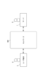
- FIG. 1 is a diagram showing an example of the configuration of an information processing system including a server which is an embodiment of an information processing device of the present invention.
- the information processing system shown in FIG. 1 is configured such that a server 1 managed by an administrator S and a user terminal 2 managed by a user U are connected to each other so that they can communicate with each other via a specified network NW.
- Server 1 is an information processing device such as a computer, which inputs trait data indicating a material structure (trait data on a predetermined scale) and outputs trait data (trait data on a smaller scale than the input trait data) that shows a better index score than the input in a statistical indicator indicating the material's characteristics. Specifically, in response to a conversion request from the user terminal 2, the server 1 converts data on the macro-scale uneven shape of, for example, the material surface into data on the uneven shape of, for example, an atomic scale and outputs the data to the user terminal 2.
- the user terminal 2 is, for example, an information processing device such as a computer, a smartphone, a tablet terminal, etc.
- the user terminal 2 makes a conversion request to the server 1 to convert data of the macro-scale uneven shape of the material surface into data of, for example, an atomic-scale uneven shape, and in response to the conversion request, obtains the converted atomic-scale uneven shape data from the server 1 and displays it on the screen.
- FIG. 2 is a block diagram showing an example of the hardware configuration of a server in the information processing system of FIG. 1.
- the server 1 includes a CPU (Central Processing Unit) 11, a ROM (Read Only Memory) 12, a RAM (Random Access Memory) 13, a bus 14, an input/output interface 15, an input unit 16, an output unit 17, a memory unit 18, a communication unit 19, and a drive 20.
- a CPU Central Processing Unit
- ROM Read Only Memory
- RAM Random Access Memory
- the CPU 11 executes various processes according to programs recorded in the ROM 12 or programs loaded from the storage unit 18 to the RAM 13. In executing the processes, in addition to the CPU, an accelerator (such as a GPU (Graphics Processing Unit)) can be used as necessary.
- the RAM 13 also stores data and the like required for the CPU 11 to execute various processes as appropriate.
- the CPU 11, the ROM 12, and the RAM 13 are interconnected via a bus 14.
- An input/output interface 15 is also connected to the bus 14.
- An input unit 16, an output unit 17, a storage unit 18, a communication unit 19, and a drive 20 are connected to the input/output interface 15. Even when an accelerator is used, it is connected to the bus 14 so as to enable mutual instruction with the CPU 11 and access to the memory unit 18 and the like.
- the input unit 16 is, for example, a device such as a keyboard or a mouse equipped with various hardware buttons, and inputs various information in response to instructions from an operator.
- the input unit 16 also includes a measuring instrument such as an atomic force microscope (AFM).
- the AFM measures the fine surface of the material (substance) to be measured, and obtains data on the uneven shape (characteristic data indicating the material structure) on a predetermined scale (e.g., macroscale or smaller).
- the data on the uneven shape of the material surface obtained by the AFM is stored in the memory unit 18.
- the output unit 17 is configured with a display such as a liquid crystal display, and displays various images.
- the storage unit 18 is configured with a dynamic random access memory (DRAM) or the like, and stores various data.
- the communication unit 19 controls communication with other devices (for example, the user terminal 2) via a network NW including the Internet.
- the drive 20 is provided as necessary.
- Programs read from the removable media 21 by the drive 20 are installed in the storage unit 18 as necessary.
- the removable media 21 can also store various data stored in the storage unit 18 in the same way as the storage unit 18.
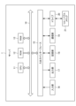
- FIG. 3 is a functional block diagram showing an example of the functional configuration of the server in FIG.
- the memory unit 18 of the server 1 stores a learning model 41 constructed (generated and updated) by the learning unit 32 .
- the learning model 41 uses a predetermined algorithm that generates output data indicating the structure of a material, which shows a better index score in a statistical index indicating the characteristics of the material than input data indicating the structure of the material. For example, a self-affine rule or the like is adopted as the predetermined algorithm.
- the self-affine law is a law of similarity of shapes at different scales, and can be adopted for data generation in this embodiment that targets materials (data conversion such as improving the image quality of the original image, removing or reducing noise, data complementation, and reducing image quality).
- a data generation unit 31 functions when executing the data generation process.
- the data generation unit 31 functions as a data generation means by exchanging data with a learning model 41 stored in the storage unit 18.
- the data generation means includes the data generation unit 31 and the learning model 41.
- the data generation unit 31 inputs trait data to be upscaled to the learning model 41, thereby causing the learning model 41 to output trait data of a smaller scale. Specifically, the data generation unit 31 acquires data on the uneven shape of the material surface that indicates the structure of a specified material, inputs the data as input data to the learning model 41, generates data on the uneven shape of the material surface on a small scale (e.g., atomic scale) that indicates the structure of the specified material output from the learning model 41, and outputs the data to the user terminal 2. That is, the data generating unit 31 acquires data on the macro-scale uneven shape, and generates and outputs data on the small-scale (for example, atomic scale) uneven shape as output data.
- a small scale e.g., atomic scale
- the data acquired by the data generating unit 31 is called first trait data
- the data output by the data generating unit 31 is called second trait data.
- the data generation means can generate trait data having a greater "amount of data on material structure per unit space” than the first trait data and output it as the second trait data (the part marked with the symbol 101 in the graph in Figure 11, the graph at the bottom of Figure 22, the graph in Figure 26, etc.).
- the output data has a better index score (higher "amount of material structure data per unit space") in terms of a statistical index indicating the characteristics of the material (“amount of material structure data per unit space”) than the input data.
- the data generation means can generate trait data in which the "power spectral density of material structure" is closer to the theoretical value than the first trait data, and output this as the second trait data (the part marked with the symbol 101 in the graph in Figure 11, the graph at the bottom of Figure 22, the graph in Figure 26, etc.).
- the output data is a statistical index ("power spectrum density of material structure") that indicates the characteristics of the material and has a better index score ("power spectrum density of material structure” is closer to the theoretical value) than the input data.
- the theoretical value is, for example, literature on material properties, appropriate analysis results and experimental results sufficient to grasp the material properties, etc.
- an algorithm can be used that uses an approximation line of the power spectral density in double logarithm of the "power spectral density of material structure" (part 101 of the graph in FIG. 11, the graph at the bottom of FIG. 22, the graph in FIG. 26, etc.).
- the output data has a better index score (the approximation line of the power spectral density in double logarithm of the power spectral density of the material structure) indicative of the characteristics of the material than the input data. This is because the output data has a better index score (the approximation line of the power spectral density in double logarithm of the power spectral density of the material structure is closer to the theoretical value) than the input data.
- a straight line can be used as the approximation line, and an algorithm can be employed that uses the slope of the straight line of the "power spectral density of material structure" (the graph on the right side of FIG. 11, the portion indicated by reference numeral 101 in the graph of FIG. 11, the graph at the bottom of FIG. 22, the graph of FIG. 26, etc.).
- the output data is a statistical index ("power spectral density of material structure") that indicates the characteristics of the material and has a better index score (the slope of the approximation line of the "power spectral density of material structure" is closer to the theoretical value) than the input data.
- the data generation means when an algorithm is adopted that uses the "amount of missing data per unit space" as a statistical indicator, the data generation means generates trait data having a smaller “amount of missing data per unit space” than the first trait data and outputs it as the second trait data (see Figures 23, 24, 25, etc.). In this case, the output data has a better index score (less "missing data per unit space") than the input data in terms of a statistical index (“amount of missing data per unit space”) that indicates the characteristics of the material.
- an algorithm can be employed that uses the "amount of noise per unit space" as a statistical index.
- This algorithm uses, as the "amount of noise per unit space," an amount that can be defined by a physical operation when acquiring the first trait data (see FIG. 28).
- the data generating means can generate trait data having a smaller "amount of noise per unit space” than the first trait data and output it as the second trait data.
- an algorithm can be adopted that uses the amount of white noise when the first trait data is acquired as the "amount of noise per unit space" (see Figure 29).
- the output data has a better index score (less "amount of noise per unit space") in a statistical index ("amount of noise per unit space”) indicating the characteristics of the material than the input data.
- the data generation means can generate and output, as the second trait data, trait data in which the "local unevenness of material structure" is closer to a theoretical value or an actual measured value than the first trait data.
- the output data is a statistical index ("local unevenness of material structure") that indicates the properties of the material and has a better index score ("local unevenness of material structure" is closer to the theoretical value or the actual measured value) than the input data.
- the actual measured value is, for example, an appropriate analysis result or experimental result that is sufficient to grasp the material properties of an individual sample.
- the data generation means can generate and output, as the second characteristic data, characteristic data in which the "surface roughness of the material surface” is closer to the theoretical value or actual measured value than the first characteristic data.
- the output data has a better index score (the "surface roughness of the material surface” is closer to the theoretical value or the actual measured value) than the input data for a statistical index indicating the characteristics of the material (the "surface roughness of the material surface”).
- the data generation means can generate and output, as the second trait data, trait data in which the "image evaluation index when the material surface is treated as a two-dimensional image” is closer to the theoretical value or actual measured value than the first trait data.
- the output data has a better index score (the "image evaluation index when the material surface is viewed as a two-dimensional image") in terms of a statistical index indicating the characteristics of the material than the input data (the "image evaluation index when the material surface is viewed as a two-dimensional image” is closer to the theoretical value or the actual measured value).
- the learning unit 32 functions when executing the learning process.
- the learning unit 32 uses teacher data as necessary to construct (create and update) a learning model 41 in the storage unit 18.
- the learning unit 32 constructs a learning model 41 that receives input data and outputs output data by machine learning the local structure of the material structure. Through the above process, the learning process of this embodiment can be executed.
- the learning unit 32 first constructs a learning model 41 (first machine learning model) that outputs output data when input data is input by performing learning on an arbitrary material structure. After that, the learning unit 32 reads the learning model 41 and performs learning on a material structure different from the initially targeted material structure, thereby constructing an updated learning model 41 (second machine learning model).
- Changing the material structure targeted by the first machine learning model and the second machine learning model can, for example, efficiently learn the characteristics of general metals and the characteristics of a specific metal by constructing a second machine learning model trained on a narrow range of material structures, such as a specific metal, for a first machine learning model trained on a wide range of material structures, such as metals in general.
- the algorithm is an algorithm that uses an updated learning model 41 (second machine learning model), and the data generation means inputs the first trait data (output of the first machine learning model) as input data into the updated learning model 41 (second machine learning model), and as a result, outputs the output data obtained from the updated learning model 41 as the second trait data (output of the second machine learning model).
- FIG. 4 is a flow chart showing the operation of the server shown in FIGS.
- step S1 the data generation unit 31 of the server 1 receives a request to convert the material structure data from the user terminal 2.
- the material structure data includes, for example, the uneven shape of the macro-scale material surface, and data measuring the uneven shape of the material surface, data on the material structure artificially generated by programming, etc. can be used.
- step S2 the data generating unit 31 acquires data on the macro-scale uneven shape from the user terminal 2 or the storage unit 18, and generates data including a more precise uneven shape (fine uneven shape) as output data.
- data on the macro-scale uneven shape from the storage unit 18 data on the macro-scale uneven shape measured by the AFM, or data on the macro-scale uneven shape artificially created by programming or the like, is stored in advance in the storage unit 18.
- the precise uneven shape is a small scale, and in principle, is a shape that is correct or plausible as the uneven shape of the material surface.
- first characteristic data e.g., data on a macro-scale uneven shape
- second characteristic data e.g., data on uneven shape with a minimum resolution of 1/4 that of the first characteristic data
- the learning model 41 includes a predetermined algorithm for generating data showing a better index score in a statistical index indicating the characteristics of a material than input data indicating the structure of the material, the data being smaller in scale than the macro-scale uneven shape data (input data) indicating the structure of the material.
- the data generating unit 31 inputs the macro-scale uneven shape data to the learning model 41, and generates small-scale (e.g., atomic scale) uneven shape data output from the learning model 41 as output data.
- step S3 the data generation unit 31 outputs the generated data of the more precise uneven shape to the requesting user terminal 2.
- FIG. 5 is a diagram showing an example of a situation in which the servers of FIGS. 2 and 3 are expected to be used.
- the server 1 As a result of the manufacture or use of industrial equipment and devices, automobiles, steel materials, etc., the structure of an arbitrary material 51 is generated as shown in Fig. 5.
- the unevenness of the material surface of an individual sample is measured using an atomic force microscope (AFM) or the like, and visualized or quantified.
- AFM atomic force microscope
- the quality of visualization and quantification depends on the specifications of the measuring equipment and the environment, and generally, the only solution is to analyze the measurement data obtained by the measuring equipment, i.e., the data on the uneven shape of the material surface itself, and it has been difficult to ensure resolution at smaller scales, such as the atomic scale or close to it.
- measuring instruments such as a scanning tunneling microscope (STM) are capable of performing measurements with atomic-scale resolution, but the measurement range is limited, making it difficult to observe various phenomena occurring in the context of material use.
- the server 1 receives as input data 52 of the uneven shape of the material surface on a coarse scale measured by a measuring instrument, and executes a data generation process to predict (predict) data 53 of the unevenness of the material surface at a resolution finer than the measurement resolution from the data 52 of the uneven shape of the material surface on a coarse scale.
- the data 52 of the rough-scale uneven shape of the material surface and the data 53 of the fine-resolution unevenness of the material surface in Fig. 5 each indicate height on a two-dimensional surface by light and dark colors. This is the same for the subsequent figures.
- the server 1 if the data on the uneven shape of the material surface is, for example, a two-dimensional image, by inputting low-resolution property data to the server 1, it is possible to cause the server 1 to output high-resolution property data.
- FIG. 6 is a diagram showing an outline of measurement by, for example, an atomic force microscope (AFM) as a measuring instrument that inputs measurement data to the servers in FIGS.
- AFM atomic force microscope
- FIG. 6A shows the measurement principle of an atomic force microscope (AFM), which is one such measuring device.
- AFM when a needle-shaped tip (probe) is placed near the surface of a material, the unevenness of the surface is measured by sensing the stress experienced when in contact, or the deformation of the tip or the cantilever connected to the tip due to atomic forces when not in contact. As shown in FIG.
- FIG. 7 is a diagram showing a fractal graph and a self-affine graph as examples of uneven shapes on a material surface.
- FIG. 8 is a diagram showing amplitude and period for considering what waveform components can constitute the unevenness when quantifying the unevenness on the material surface.
- the amplitude with respect to scale is equal when the unevenness is observed on a wide scale and when it is observed on a narrow scale.
- the amplitudes at large and small scales are correlated, though not necessarily equal, i.e., the amplitude decreases proportionally from large to small scales.
- the period and amplitude are defined, for example, as shown in FIG. 8. Based on these, the energy per unit length relative to the magnitude of the frequency (1/period) can be obtained.
- PSD power spectral density
- a line graph for example, as shown in FIG. 9, with the horizontal axis representing frequency and the vertical axis representing power relative to the magnitude of the frequency (Signal 2 /Frequency).
- a double logarithmic graph is used as an example of a line graph.
- the PSD allows analysis of frequency components in the spatial domain.
- FIG. 9 is a diagram showing an example of line graphs of PSD for fractal and self-affine.
- the PSD on the vertical axis is constant regardless of the frequency on the horizontal axis.
- the self-affine line graph as the Frequency decreases, the PSD also decreases, and this tendency can be said to be in a proportional relationship when both the vertical and horizontal axes are plotted in logarithmic (log) scales.
- FIG. 10 is a double logarithmic graph showing a measured image of the uneven shape of a typical material surface and its PSD.
- FIG. 11 is a double logarithmic graph showing a measured image of the uneven shape of a material surface when the measurement resolution is higher than that of the measurement in FIG. 10 (in the case of a thin chip) and its PSD.
- the amount of information contained in the material surface unevenness data increases due to the small pixel size. More specifically, when considering what waveform components can constitute unevenness, fine waveform components can also be detected due to the high resolution. Therefore, with PSD, it is possible to add plots for low frequency regions.
- the waveform component of high resolution can be represented not only by the line (proportional relationship) of the uneven shape of a typical material surface shown in FIG. 10, but also by line segment 101 in the line graph of FIG. 11, which is an extension of the line in FIG. 10 further in a lower right direction.
- the algorithm of learning model 41 which generates output data indicating the structure of a material that shows a better index score in a statistical indicator indicating the characteristics of the material than the input data indicating the structure of the material, can use, for example, the "power spectral density of the material structure" as a statistical indicator, and generate and output trait data in which the "power spectral density of the material structure" is closer to the theoretical value than the original trait data.
- the theoretical value of the "power spectral density of the material structure” an approximation line (straight line) of the power spectral density in double logarithm can be used.
- a straight line is used as the approximation line, and an example of a good index score is one in which the "power spectral density of the material structure" indicated by any data is close to the slope of a straight line considered to be the theoretical value of the material, and also, for example, one in which the "power spectral density of the material structure” indicated by any data is close to the section of the straight line (length of the straight line region) considered to be the theoretical value of the material.
- FIG. 12 is a diagram showing an example of how a learning model is used in the server of this embodiment.
- the above-mentioned learning model 41 is used in two steps, a training step S21 and an inference step S22, as shown in FIG.
- the training step S21 is a step of training the learning model 41 using the input data 121 and the intermediate data 122.
- the inference step S22 is a step of performing inference using the input data 123 and the learning model 41 resulting from training, and output data 124 can be obtained as the inference result.
- input data 121 is input.
- the input data 121 is low resolution data.
- the training step S21 includes a conversion step S31 (pre-convert).
- the conversion step S31 converts the input low-resolution data into high-resolution data (High resolution), which is intermediate data 122.
- This conversion process may be a procedure in which intermediate high-resolution data is prepared first, and then the conversion step S31 obtains the input low-resolution data.
- the learning model 41 is trained (the model is updated through learning). This enables the learning model 41 to learn the process of converting low-resolution data into high-resolution data, in other words, the data generation step of generating data on the uneven shape of a micro-scale material surface.
- the input data 121 used for training may be one or more measurement data (e.g., one or more images), but a large number (e.g., hundreds to tens of thousands) is preferable. In addition, it is not necessary to use the entire range of measured data for one piece of data, and partial use is also acceptable. By partially using different parts of one piece of data, it is also possible to treat it as the amount of data for multiple pieces of data. For deep learning, a method that can learn the characteristics of data is preferable, and for example, a GAN (generative adversarial network) can be used.
- GAN generative adversarial network
- one low-resolution data is input as input data 123 to the post-training learning model 41.
- the learning model 41 converts the input data 123 into high-resolution data and outputs it.
- the learning model 41 which has learned the process of generating micro-scale material surface irregularities, to any low-resolution data, the micro-scale material surface irregularities are added to the low-resolution data, and it is output as high-resolution data.
- the low-resolution data at this time is basically assumed to be data that was not used in the training step S21, in order to make it easier to avoid over-learning in the high-resolution of localized irregularities, but it may also be data that was used in the training step S21.
- the data used as input for inference step S22 is first analyzed, and then a large amount of data similar to that data (essentially the same but randomly different) is artificially created and used for training.
- the surface of a ceramic can be measured with an AFM, the slope of a log-log graph of the PSD can be calculated from the measurement results, and new data matching that slope can be generated using a program, etc.
- literature on material properties can be cited, and new data matching the desired characteristics can be generated using a program, etc. This method can reduce the number of measurements and increase the amount of training data, improving the accuracy of machine learning.
- the training step S21 only requires a function to learn the generation process of micro-scale material surface irregularities from known low-resolution data, and the inference step S22 only requires a function to apply any constructed learning model 41 to any low-resolution data.
- training step S21 can be performed at 512 x 512 pixels instead of 64 x 64 pixels
- inference step S22 can be performed at 1024 x 1024 pixels instead of 128 x 128 pixels.
- FIG. 13 is a diagram showing a conversion step for converting low-resolution data into high-resolution data in the server of this embodiment.
- intermediate high-resolution data can be generated based on the input low-resolution data in accordance with separately set constraints.
- low resolution input data of data size L corresponds to the line 131 at the top left of the plot
- simulated high resolution data of data size Ls corresponds to the line 132 at the bottom right of the graph.
- the constraints are, for example, the slope of the log-log plot of the PSD and the pixel conversion scale (for example, 1/4 when 1 ⁇ 1 pixel of input data is converted to 4 ⁇ 4 pixel of output data).
- the slope of the log-log plot indicates the "dimension of the material surface irregularities according to the resolution.” In other words, by determining the pixel conversion scale, the dimensions of the material surface irregularities when the input data is converted into data of a different pixel size can be scaled and calculated using values that conform to the self-affine.
- one example of a calculation method that can be used by the server 1 is a method of scaling before and after conversion, assuming that the PSD (C 2D ) of a two-dimensional image is C 2D ⁇ h 2 A ⁇ 1 , where h is the height of the unevenness and A is the area of interest (Non-Patent Document (ACS Appl. Mater. Interfaces 10, (2016) 29169)).
- Indicators equivalent to constraints such as intermediate values in the above calculation process may be manually input by the server 1, or may be calculated from the input data.
- a method may be used in which a log-log plot of the PSD against the input data is first made, an approximation line is found using the least squares method or the like, and the slope is then calculated.
- FIG. 14 shows a case where the conversion step (pre-convert) is performed in the reverse order to that shown in FIG. 13, and is a diagram showing the conversion steps for converting high-resolution data into low-resolution data in the server of this embodiment.
- the input low-resolution data can be generated from the intermediate high-resolution data previously prepared by a method generally used for image processing or the like.
- the nearest neighbor method can be used as a method for image processing.
- the nearest neighbor method can be used.
- the nearest neighbor method is used, if the pixel conversion scale is 4, the low-resolution data of the input data can be created by converting the 4 ⁇ 4 pixels of the high-resolution data prepared in advance into 1 ⁇ 1 pixels (see FIGS. 14A and 14B).
- the image size of the known high-resolution data in real space is virtually enlarged, and the scale when it is enlarged in real space is calculated in the reverse order of the calculation in FIG. 13, thereby generating low-resolution data (see FIGS. 14C and 14D).
- FIG. 15 is a diagram illustrating an example of the configuration of a deep learning function of a learning model constructed by a learning unit.
- the deep learning function of the learning model constructed by the learning unit includes a generator 151 (G) and a discriminator 152 (D).
- a GAN When a GAN is used in deep learning, the input low-resolution data is input to a generator 151 (G), and the output of the generator 151 (G) and the intermediate high-resolution data are input to a discriminator 152 (D).
- the input data is 64 x 64 pixels and the final output data is 512 x 512 pixels
- the input data is first accepted and converted to 512 x 512 pixels, and then input to generator 151 (G).
- the conversion at this time may be performed using bilinear interpolation, bicubic interpolation, nearest neighbor interpolation, or the like, or 1 x 1 pixel of the 64 x 64 pixel image may simply be copied across 8 x 8 pixels of the 512 x 512 pixels.
- the generator 151(G) generates simulated high-resolution data from an input of 512 ⁇ 512 pixels based on an arbitrary process, and outputs the data in 512 ⁇ 512 pixels. At this stage, the 512 ⁇ 512 pixel data filled with values that are the same as or close to the 64 ⁇ 64 pixel input data is rewritten with 512 ⁇ 512 pixel data that is different from the input data.
- the output of generator 151(G) is input to discriminator 152(D) along with the intermediate high resolution data (512 ⁇ 512 pixels) shown in FIGS.
- a discriminator 152 (D) compares the output of the generator 151 (G) with the intermediate high-resolution data based on an arbitrary process, and outputs the match between the two. Taking into account the results of the matching, the generator 151 (G) repeatedly learns according to the number of epochs so that the simulated high-resolution data it outputs matches more closely with the intermediate high-resolution data, and the discriminator 152 (D) repeatedly learns according to the number of epochs so as to more accurately compare the two so as to be able to discern the simulated high-resolution data.
- the generator 151 (G) learns the process of converting input low-resolution data (64 x 64 pixels) into high-resolution data (512 x 512 pixels).
- FIG. 16 is a diagram illustrating an example of the configuration of a generator (G) of the learning model in FIG.
- FIG. 17 is a diagram showing an example of the configuration of a classifier (D) in the learning model of FIG.
- the generator (G) shown in FIG. 16 and the discriminator (D) shown in FIG. 17 can use a publicly known or unique learning model that combines processes such as convolution.
- the generator 151 (G) and the discriminator 152 (D) can be configured by combining processes such as convolution (Conv), activation (Act), batch normalization (BN), summation (Sum), pixel shuffle (PS), and dense (Den).
- FIG. 18 is a flowchart (part 1) showing the learning process of the generator 151 (G) in FIG. 16 and the discriminator 152 (D) in FIG.
- FIG. 19 is a flowchart (part 2) showing the learning process of the generator 151 (G) in FIG. 16 and the discriminator 152 (D) in FIG.
- step P0 the operation begins and the data set is read.
- step P1 mini-batches are generated from the dataset.
- step P2 the generator 151(G) reads the mini-batch data.
- step P3 the generator 151(G) generates simulated high-resolution data.
- step P4 the loss function is calculated and the generator 151 (G) is updated.
- step P5 it is determined whether the upper limit of the mini-batch has been reached. If the result of the determination is that the upper limit of the mini-batch has been reached, the process transitions to step P6, and if not, the process transitions to step P2.
- step P6 the generator 151(G) determines whether or not the set number of epochs has been reached. If the result of the determination is that the set number of epochs has been reached, the process proceeds to step M1, and if not, the process proceeds to step P1.
- step M1 we generate mini-batches from the dataset.
- step M2 the generated mini-batch data is read.
- step M3 the generator 151(G) executes a process of generating simulated high-resolution data using the read mini-batch.
- step M4 the discriminator 152(D) executes a process of comparing the generated high-resolution data with known high-resolution data (intermediate high-resolution data).
- step M5 the loss function is calculated and the generator 151 (G) is updated.
- step M6 the loss function is calculated and the discriminator 152(D) is updated.
- step M7 it is determined whether the upper limit of the mini-batch has been reached.
- step M8 it is determined whether or not a best score has been derived for any index. As a result of the determination, if a best score has been derived for any index, the process proceeds to step M9, and if not, the process proceeds to step M10.
- step M9 the generator 151(G) is saved.
- step M10 it is determined whether or not the set number of epochs has been reached. If it is determined that the set number of epochs has been reached, the process proceeds to step M11; if not, the process proceeds to step M1. In step M11, the operation ends.
- the number of data and the batch size may be any scale, but the number of data is preferably 1000 or more, and more preferably 5000 or more, to improve the accuracy of the learning model 41.
- a batch size of 8 to 64, and more preferably 16 to 32, is preferable because it is easy to balance the learning speed and the accuracy of the learning model 41.
- the number of epochs may be of any scale, but is preferably 50 or more, and more preferably 100 or more, in order to improve the accuracy of the learning model 41.
- a loss function based on a comparison between any two images can be used, such as the mean absolute error MAE, the mean squared error MSE, pixel-wise binary cross entropy, content loss/style loss, edge loss, loss based on a material-related index (such as local slope), loss based on an index commonly used in image processing (e.g. PSNR, SSIM, etc.), or adversarial loss when GAN is used.
- These losses can be used alone as a loss function, or can be used in combination as a loss function.
- the loss function of the classifier 152(D) can be a loss function that is generally used in GANs, such as binary cross entropy.
- a method in order to reduce the computational load required for learning and output more plausible high-resolution data, a method can be applied in which the results of the learning round and the learning model 41 that showed good results in any index are extracted from multiple repetitions.
- the arbitrary index may be an index related to deep learning (e.g., loss value), an index related to the trend of a PSD graph (e.g., the amount of change in PSD before and after learning), an index related to local material surface unevenness (e.g., the squared error of a contour line at a specific location before and after learning), an index commonly used in image processing, etc. (e.g., PSNR, SSIM, etc.), an index related to the accuracy of the learning model 41 in the server 1 (e.g., the remaining pixel boundaries of the original low-resolution image), etc.
- an index related to deep learning e.g., loss value
- an index related to the trend of a PSD graph e.g., the amount of change in PSD before and after learning
- FIG. 20 is a flow chart showing an inference process using the generator 151(G) of FIG.
- Step I0 indicates the start of the operation.
- the target data is read.
- a generator 151(G) created in advance is read.
- high-resolution data is predicted (estimated) using the read data and output.
- Step I4 indicates the end of the operation.
- FIG. 21 is a diagram showing an example of generating output data of 512 ⁇ 512 pixels from input data of 64 ⁇ 64 pixels in the learning model of FIG.
- FIG. 21D shows high-resolution input data (512 ⁇ 512 pixels) for comparison with the output results.
- Figure 21(D) shows ideal 2D data that follows the self-affine law
- Figure 21(A) shows Figure 21(D) with reduced resolution; both were used as equivalent to measured data.
- Figure 21(B) shows an example of the results of learning based on CNN, a common deep learning method.
- the PSD trends show a tendency close to the input data, but do not resemble the high-resolution data.
- FIG. 21C shows an example result based on GAN (using at least adversarial loss) on server 1, and it can be seen that the PSD progression shows a similar trend to the high-resolution data.
- the numerical value for the comparative example in FIG. 21(D) is ⁇ 0.001966
- the numerical value for FIG. 21(C) is ⁇ 0.001961, showing values that are close to each other.
- a known estimation method can be used to plot the PSD from two-dimensional data of the material surface unevenness, such as the Periodogram method or the Welch method.
- the Periodogram method or the Welch method.
- a total of four cases are plotted, including the Periodogram method and the Welch method in which the segment division parameters are divided into three cases.
- the slope of the plot data estimated by the Welch method in which the segment division parameter is n/8 when the output pixel size is n is used, and a linear equation is obtained by least squares approximation excluding zero points.
- the output can be used as an indicator of a better result than the input by using one or more of the following indicators: an increase in the resolution of the material's unevenness (amount of data on the material structure per unit space), an increase in the conformity of the PSD (whether it is close to the target property, such as a straight line), a decrease in the error of the PSD (whether there is less error compared to the target property, such as a straight line), etc.
- FIG. 22 is a diagram for explaining improvement in prediction accuracy in first prediction and in second or more predictions.
- the server 1 can perform a single upconversion process to increase the resolution of the uneven surface data of the material at any scale ratio, but it is not necessarily possible to increase the resolution to the atomic scale of the actual material.
- the output results up to the previous time are used as input data for the second prediction (Second Prediction) and subsequent processes, and the upconversion process is repeated multiple times, in other words, the high-resolution prediction process is executed multiple times, so that trait data on a smaller scale can be obtained as a prediction result (the extended straight line in the line graph to the right of the arrow in FIG. 22 ).
- FIG. 23 is a diagram showing a first case in which the server of the embodiment executes the complementation process when the target measurement image is thinned-out measurement data.
- the data generating unit 31 executes an interpolation process on the measurement data and outputs interpolated data 232.
- the tip (probe) of a measuring device is scanned vertically and horizontally at equal intervals to obtain the measured image 231 (two-dimensional image data) shown in Fig. 23, thinning out the horizontal scanning pitch will result in missing data.
- the data generating unit 31 operates to repair the missing data.
- an image 233 is shown in which unknown data is expressed by white squares and known data is expressed by filled squares in each pixel of the measurement image 231 shown in FIG.
- Data in which half the data has been thinned out horizontally can be converted into unthinned low-resolution data 234 by performing low-resolution image processing.
- this can be achieved by converting 2x2 pixels into 1x1 pixels, and one or both of the two known pieces of data from the 2x2 pixels can be used.
- the low-resolution data 234 is converted to high quality (up-converted) by the data generation unit 31, and as a result, high-resolution data 235 is output. This is equivalent to generating data to fill in the thinned areas of the original measurement data and complementing those areas.
- FIG. 24 is a diagram showing a second case in which the server of the embodiment executes the complementation process when the target measurement image is thinned-out measurement data in which known and unknown locations are mixed.
- a known location and an unknown location are locations that can be distinguished depending on whether measured data exists or does not exist (data is missing) in a partial range within the image.
- the data generation unit 31 performs an interpolation process on the measurement data and outputs the interpolated data 247.
- the high-resolution part of the measurement image 241 (4 x 4 pixels) in the lower left corner, from which a relatively large amount of pixel data has been obtained
- a process 242 that converts 2 x 2 pixels to 1 x 1 pixel can be used to obtain interpolated data 243 that covers the entire area of interest.
- new data 244 can be generated across 8 ⁇ 8 pixels by applying the interpolated data 243 to the original measured image 241.
- the 8 ⁇ 8 pixels can be converted into 4 ⁇ 4 pixel low-resolution data 245 by converting each 2 ⁇ 2 pixel portion into 1 ⁇ 1 pixel.
- the data 245 can be made high-resolution using the same procedure as described above.
- the output of the up-conversion process is then obtained as 8 ⁇ 8 pixel predicted data 246.
- an indicator of whether the output is better than the input can be whether the amount of missing data per unit space is reduced compared to the input.
- FIG. 25 is a diagram showing a third case in which the measurement data range is expanded for measurement data of a unique example in which known locations and unknown locations are mixed.
- a process for complementing the missing portion can be performed in a similar manner to that described above, thereby generating data on the unevenness of the material surface in which the missing portion has been repaired.
- the data generation unit 31 can generate trait data with a smaller "amount of missing data per unit space" than the first trait data and output it as the second trait data.
- a learning model 41 as an algorithm that adopts the "amount of missing data per unit space" as a statistical indicator
- the data generation unit 31 can generate trait data with a smaller "amount of missing data per unit space" than the first trait data and output it as the second trait data.
- FIG. 26A and 26B show log-log graphs of the PSD of unevenness data on a material surface
- FIG. 26(A) shows a log-log graph of the PSD of unevenness data on a micro-scale material surface generated according to the self-affine law.
- the plot of the log-log graph of PSD is a straight line sloping downward to the right, with the upper left portion 261 representing the input data and the lower right portion 262 representing the predicted data predicted from the input data.
- FIG. 26B shows a log-log plot of the PSD when any material surface does not follow the self-affine law and exhibits a curvilinear trend in the PSD.
- FIG. 26C shows a log-log graph of the PSD when an arbitrary material surface does not follow equal self-affine laws along each axis in two dimensions, but shows self-affine laws with different degrees along each axis. Even when the slope of the PSD differs on the x and y axes of a two-dimensional image, as in the double logarithmic graph shown in FIG. 26C, the data generating unit 31 can generate data with high image quality.
- the uneven shape data of a two-dimensional material surface can be expressed on two axes, x (direction 1) and y (direction 2), and shows different PSD gradients
- different constraints can be set for direction 1 and direction 2 to predict the high-resolution data.
- the learning process can be divided into direction 1 and direction 2, and for example, the output obtained after completing the prediction for direction 1 first can be used as input for the prediction for direction 2.
- indices other than PSD such as whether local unevenness is close to the actual measured value, whether surface roughness is close to the actual measured value, whether the image evaluation index (e.g. PSNR, SSIM, etc.) when the material surface is treated as a two-dimensional image, etc. may also be used.
- the data generation unit 31 can generate and output unevenness shape data (second characteristic data) in which the “local unevenness of the material structure” is closer to the actual measured value than the unevenness shape data of the measured two-dimensional material surface.
- the learning model 41 which is an algorithm that employs the “surface roughness of the material surface” as a statistical indicator
- the data generation unit 31 can generate and output unevenness shape data (second characteristic data) in which the “surface roughness of the material surface” is closer to the actual measured value than the unevenness shape data of the measured two-dimensional material surface.
- the data generation unit 31 can generate and output unevenness shape data (second characteristic data) in which the "image evaluation index when the material surface is treated as a two-dimensional image” is closer to the actual measured value than the unevenness shape data of the measured two-dimensional material surface.
- these indices may be set with reference to the properties of the actual material (classification such as metal or ceramic, state of surface treatment such as polishing), or they may be set by analyzing data from actual material samples and finding the index with the highest matching from the differences observed when the device is run on a small scale (small amount of data or short number of runs).
- the log-log graph of the PSD generally follows a straight line sloping downward to the right, so the slope of the PSD can be set as an index.
- the target indicators can be set to change as the learning process progresses, and the learning process can be designed to ultimately satisfy multiple indicators.
- a three-dimensional structure can be output. It can also be applied to structures other than materials (such as the shapes and geometric patterns of plants that satisfy the self-affine law).
- FIG. FIG. 27 is a diagram for explaining the mechanism by which physical noise occurs when measuring unevenness data (characteristic data) on a material surface.
- FIG. 28 is a diagram showing an example of trait data that differs depending on whether or not physical noise occurs.
- FIG. 28A shows an example of trait data in which no physical noise occurs
- FIG. 28B shows an example of trait data in which physical noise occurs.
- a needle-shaped tip 271 is lowered in the direction of arrow 272 and brought close to the material surface 273 to sense (measure) the unevenness of the material surface 273.
- this is a physical operation in which the tip 271 (probe) traces the unevenness of the material surface.
- tip tip 271a (lowest point) does not necessarily come into contact with material surface 273 because tip tip 271a has a finite size (when enlarged, the tip tip has a hemispherical shape).
- a side surface 274 of a tip 271a of the tip is in contact with a material surface 273, and the height of the tip 271a at this time is sensed as a position 275 on the material surface 273 for measurement purposes.
- the measured position 275 differs from the position 276 of the true material surface 273, and performing similar sensing across the entire material surface would result in noisy measurements.
- Data (characteristic data) of the uneven shape of the material surface that does not contain physical noise is obtained as noise-free data as shown in Figure 28 (A), whereas data of the uneven shape of the material surface that contains physical noise, obtained as a result of the sensing in Figure 27 above, is output as data with physical noise as shown in Figure 28 (B).
- a learning model 41 which is constructed by adopting, as a statistical index, the amount of noise which can be defined by the physical operation of a tip (probe) tracing the unevenness of the material surface, thereby making it possible to generate unevenness data on the material surface with less noise.
- a learning model 41 constructed by learning the relationship between trait data containing physical noise and trait data in a high-resolution state that does not contain noise using multiple samples it is possible to predict high-resolution trait data that does not contain physical noise even from input data that contains physical noise, and therefore it is possible to convert the input data containing noise in accordance with the prediction, and generate and output high-resolution data with reduced noise.
- FIG. 29A and 29B show the difference in data depending on whether or not white noise is present.
- FIG. 29A shows data on the uneven shape of a material surface without noise
- FIG. 29B shows data on white noise
- FIG. 29C shows data on the uneven shape of a material surface including white noise.
- White noise is noise that is statistically uniformly applied to the measurement range. For example, when the white noise of FIG. 29(B) is applied to the uneven shape data of FIG. 29(A), it is replaced with data such as that shown in FIG. 29(C).
- the data generation unit 31 can generate and output data on the uneven shape of the material surface (second characteristic data) that has a smaller “amount of noise per unit space” than the data on the uneven shape of the measured material surface (first characteristic data).
- indicators that show that the output is better than the input can include indicators such as whether the amount of noise per unit space is small (the noise in this case being an amount that can be defined by physical operations, the amount of white noise, etc.).
- FIG. 30 is a diagram illustrating an example of the configuration of a server according to an embodiment when executing data conversion processing after fine tuning of the learning model 41.
- the server 1 may perform the training step not only once, but also two or more times, using a known fine-tuning method.
- the learning model 41 learns the data set [1] in the first training step, and learns the data set [2] in the second training step. By performing a certain amount of training on dataset [1], dataset [2] can output highly accurate results even with a small amount of data.
- a large dataset of similar materials [1] is prepared and a first training run is performed. Then, for samples whose data is difficult to obtain, a smaller dataset [2] is prepared and a second training run is performed, allowing this device to be used even when there are only a small number of target samples.
- the indicators from the perspectives mentioned above can be used as indicators that show a better result in the output than in the input.
- various indices can be used, as necessary, in accordance with the method of extracting good results shown in the processing steps executed by server 1, such as whether the indices defining the uneven shape of the material surface are good (whether the local unevenness is close to the actual measured value, whether the surface roughness is close to the actual measured value, etc.), whether the image evaluation indices (PSNR, SSIM, etc.) when the material surface is treated as a two-dimensional image are good, etc.
- the series of processes described above can be executed by hardware or software.
- the functional configuration in FIG. 3 is merely an example and is not particularly limited. That is, it is sufficient that the information processing device is provided with a function capable of executing the above-mentioned series of processes as a whole, and the type of functional block used to realize this function is not limited to the example of Fig. 3.
- the location of the functional blocks and database is not particularly limited to that of Fig. 3 and may be arbitrary.
- at least a part of the functional blocks and database required for executing various processes may be transferred to a user terminal or the like.
- the functional blocks and database of the user terminal may be transferred to a server or the like.
- one functional block may be configured as a single piece of hardware, a single piece of software, or a combination of both.
- the program constituting the software is installed into a computer or the like from a network or a recording medium.
- the computer may be a computer implemented with dedicated hardware.
- the computer may be a computer capable of executing various functions by installing various programs, such as a server, a general-purpose smartphone, or a personal computer.
- the recording medium containing such a program may be configured not only as a removable medium (not shown) that is distributed separately from the device body in order to provide the program to the user, but also as a recording medium that is provided to the user in a state where it is already installed in the device body.
- the steps of describing a program to be recorded on a recording medium include not only processes that are performed chronologically according to the order, but also processes that are not necessarily performed chronologically but are executed in parallel or individually.
- the term "system” refers to an overall device that is composed of a plurality of devices, a plurality of means, etc.
- an information processing device to which the present invention is applied it is sufficient for an information processing device to which the present invention is applied to have the following configuration, and various embodiments can be adopted.
- an information processing device to which the present invention is applied for example, the server 1 in FIG. 3
- a data generating means e.g., the data generating unit 31 and the learning model 41 in FIG.
- first property data e.g., data on the uneven shape of the material surface at a macro scale
- second property data e.g., data on the uneven shape of the material surface at an atomic scale
- the predetermined algorithm (e.g., the algorithm of the learning model 41) is an algorithm that adopts “amount of data of material structure per unit space” as the statistical index
- the data generating means (e.g., the data generating unit 31 and the learning model 41 in FIG. 3) generates and outputs, as the second trait data, trait data having a larger "amount of data of material structure per unit space" than the first trait data (e.g., the portion indicated by reference numeral 101 in the graph in FIG. 11, the graph at the bottom of FIG. 22, the graph in FIG. 26, etc.), It is possible.
- the predetermined algorithm is an algorithm that adopts a “power spectral density of material structure” as the statistical index
- the data generating means e.g., the data generating unit 31 and the learning model 41 in FIG. 3 ) generates and outputs, as the second trait data, trait data in which the “power spectral density of material structure” is closer to a theoretical value than the first trait data (e.g., the portion indicated by reference numeral 101 in the graph in FIG. 11 , the graph at the bottom of FIG. 22 , the graph in FIG. 26 , etc.), It is possible.
- the predetermined algorithm is an algorithm that uses an approximation line of the power spectral density in double logarithm as the theoretical value of the "power spectral density of the material structure" (for example, the part indicated by reference numeral 101 in the graph of FIG. 11, the graph at the bottom of FIG. 22, the graph of FIG. 26, etc.).
- the specified algorithm e.g., the algorithm of learning model 41
- the specified algorithm is an algorithm that employs a straight line as the approximation line and uses the slope of the straight line as the theoretical value of the "power spectral density of material structure" (e.g., the portion indicated by reference numeral 101 in the graph of FIG. 11, the graph at the bottom of FIG. 22, the graph of FIG. 26, etc.).
- the predetermined algorithm (e.g., the algorithm of the learning model 41) is an algorithm that adopts the “amount of missing data per unit space” as the statistical index
- the data generating means (e.g., the data generating unit 31 and the learning model 41 in FIG. 3) generates and outputs, as the second trait data, trait data having a smaller "amount of missing data per unit space" than the first trait data (e.g., see FIG. 23, FIG. 24, FIG. 25, etc.), It is possible.
- the predetermined algorithm (e.g., the algorithm of the learning model 41) is an algorithm that employs “amount of noise per unit space” as the statistical index
- the data generating means (e.g., the data generating unit 31 and the learning model 41 in FIG. 3) generates and outputs, as the second trait data, trait data having a smaller "amount of noise per unit space" than the first trait data (e.g., see FIG. 28, FIG. 29, etc.), It is possible.
- the predetermined algorithm e.g., the algorithm of learning model 41
- the predetermined algorithm is an algorithm that employs, as the "amount of noise per unit space," an amount of noise that can be defined by a physical operation (the operation of tracing the uneven shape of the material surface with a tip (probe)) when acquiring the first characteristic data (e.g., see Figures 27 and 28, etc.).
- the specified algorithm (e.g., the algorithm of learning model 41) is an algorithm that uses the amount of white noise when the first trait data is acquired as the "amount of noise per unit space" (see, for example, FIG. 29, etc.).
- the predetermined algorithm (e.g., the algorithm of the learning model 41) is an algorithm that adopts “local unevenness of a material structure” as the statistical index
- the data generating means (e.g., the data generating unit 31 and the learning model 41 in FIG. 3) generates and outputs, as the second property data, property data in which the "local unevenness of the material structure" is closer to an actual measured value than the first property data (e.g., see FIG. 26, FIG. 30, etc.), It is possible.
- the predetermined algorithm (e.g., the algorithm of the learning model 41) is an algorithm that adopts “surface roughness of a material surface” as the statistical index
- the data generating means (e.g., the data generating unit 31 and the learning model 41 in FIG. 3) generates and outputs, as the second trait data, trait data in which the "surface roughness of the material surface" is closer to an actual measured value than the first trait data (e.g., see FIG. 26, FIG. 30, etc.), It is possible.
- the predetermined algorithm (e.g., the algorithm of the learning model 41) is an algorithm that adopts an “image evaluation index when the material surface is represented as a two-dimensional image” as the statistical index
- the data generating means (e.g., the data generating unit 31 in FIG. 3) generates and outputs, as the second property data, property data in which the "image evaluation index when the material surface is made into a two-dimensional image" is closer to an actual measurement value than the first property data (e.g., see FIG. 26, FIG. 30, etc.), It is possible.
- the information processing device e.g., server 1 in FIG. 3
- a learning means e.g., the learning unit 32 in FIG. 3
- the predetermined algorithm is an algorithm that uses the machine learning model (e.g., the learning model 41 in FIG. 3 )
- the data generation means e.g., the data generation unit 31 and the learning model 41 in FIG. 3
- the information processing device e.g., server 1 in FIG. 3
- a learning means e.g., the learning unit 41 in FIG. 3
- first machine learning model e.g., the learning model 41 in FIG. 3
- second machine learning model e.g., the updated learning model 41 in FIG.
- the predetermined algorithm is an algorithm that uses the second machine learning model (e.g., the updated learning model 41 of FIG. 3 ),
- the data generation means e.g., the data generation unit 31 and the learning model 41 in FIG. 3
- An information processing method to which the present invention is applied comprises: In an information processing method executed by an information processing device (for example, the server 1 in FIG. 3), a data generation step (e.g., step S2 in FIG. 4 ) of acquiring first property data (e.g., macro-scale uneven shape data) indicating the structure of a predetermined material as input data based on a predetermined algorithm for generating output data indicating the structure of the material (e.g., atomic-scale uneven shape data, which is smaller in scale than macro-scale uneven shape data) that shows a better index score in a statistical index indicating the characteristics of the material than input data indicating the structure of the material, and generating and outputting second property data (e.g., atomic-scale uneven shape data) indicating the structure of the predetermined material as the output data; Including, It is possible.
- first property data e.g., macro-scale uneven shape data
- output data indicating the structure of the material
- second property data e.g., atomic-scale uneven shape
- a data generation step (e.g., step S2 in FIG. 4 ) of acquiring first property data (e.g., macro-scale uneven shape data) indicating the structure of a predetermined material as input data based on a predetermined algorithm for generating output data indicating the structure of the material (e.g., atomic-scale uneven shape data, which is smaller in scale than macro-scale uneven shape data) that shows a better index score in a statistical index indicating the characteristics of the material than input data indicating the structure of the material, and generating and outputting second property data (e.g., atomic-scale uneven shape data) indicating the structure of the predetermined material as the output data; Executing a control process including It is possible.
- first property data e.g., macro-scale uneven shape data
- output data indicating the structure of the material
- second property data e.g., atomic-scale uneven shape data
Landscapes
- Physics & Mathematics (AREA)
- General Physics & Mathematics (AREA)
- Engineering & Computer Science (AREA)
- Health & Medical Sciences (AREA)
- General Health & Medical Sciences (AREA)
- Nuclear Medicine, Radiotherapy & Molecular Imaging (AREA)
- Radiology & Medical Imaging (AREA)
- Computer Vision & Pattern Recognition (AREA)
- Theoretical Computer Science (AREA)
- Length Measuring Devices With Unspecified Measuring Means (AREA)
- Image Analysis (AREA)
Priority Applications (2)
| Application Number | Priority Date | Filing Date | Title |
|---|---|---|---|
| JP2025510746A JPWO2024203900A1 (https=) | 2023-03-24 | 2024-03-22 | |
| EP24780018.8A EP4675284A1 (en) | 2023-03-24 | 2024-03-22 | Information processing device, information processing method and program |
Applications Claiming Priority (2)
| Application Number | Priority Date | Filing Date | Title |
|---|---|---|---|
| JP2023-047940 | 2023-03-24 | ||
| JP2023047940 | 2023-03-24 |
Publications (1)
| Publication Number | Publication Date |
|---|---|
| WO2024203900A1 true WO2024203900A1 (ja) | 2024-10-03 |
Family
ID=92906415
Family Applications (1)
| Application Number | Title | Priority Date | Filing Date |
|---|---|---|---|
| PCT/JP2024/011391 Ceased WO2024203900A1 (ja) | 2023-03-24 | 2024-03-22 | 情報処理装置、情報処理方法及びプログラム |
Country Status (3)
| Country | Link |
|---|---|
| EP (1) | EP4675284A1 (https=) |
| JP (1) | JPWO2024203900A1 (https=) |
| WO (1) | WO2024203900A1 (https=) |
Citations (6)
| Publication number | Priority date | Publication date | Assignee | Title |
|---|---|---|---|---|
| JP2012233845A (ja) | 2011-05-09 | 2012-11-29 | Hitachi High-Technologies Corp | 磁気力顕微鏡用カンチレバーおよびその製造方法 |
| JP2018195069A (ja) * | 2017-05-17 | 2018-12-06 | キヤノン株式会社 | 画像処理装置および画像処理方法 |
| WO2021090469A1 (ja) * | 2019-11-08 | 2021-05-14 | オリンパス株式会社 | 情報処理システム、内視鏡システム、学習済みモデル、情報記憶媒体及び情報処理方法 |
| JP2021528775A (ja) * | 2018-07-03 | 2021-10-21 | ナノトロニクス イメージング インコーポレイテッドNanotronics Imaging,Inc. | 超解像イメージングの精度に関するフィードバックを行い、その精度を改善するためのシステム、デバイス、および方法 |
| WO2022008667A1 (en) * | 2020-07-08 | 2022-01-13 | Sartorius Stedim Data Analytics Ab | Computer-implemented method, computer program product and system for processing images |
| JP2022134649A (ja) * | 2021-03-03 | 2022-09-15 | 地方独立行政法人東京都立産業技術研究センター | 走査型プローブ顕微鏡、情報処理装置、およびプログラム |
-
2024
- 2024-03-22 JP JP2025510746A patent/JPWO2024203900A1/ja active Pending
- 2024-03-22 EP EP24780018.8A patent/EP4675284A1/en active Pending
- 2024-03-22 WO PCT/JP2024/011391 patent/WO2024203900A1/ja not_active Ceased
Patent Citations (6)
| Publication number | Priority date | Publication date | Assignee | Title |
|---|---|---|---|---|
| JP2012233845A (ja) | 2011-05-09 | 2012-11-29 | Hitachi High-Technologies Corp | 磁気力顕微鏡用カンチレバーおよびその製造方法 |
| JP2018195069A (ja) * | 2017-05-17 | 2018-12-06 | キヤノン株式会社 | 画像処理装置および画像処理方法 |
| JP2021528775A (ja) * | 2018-07-03 | 2021-10-21 | ナノトロニクス イメージング インコーポレイテッドNanotronics Imaging,Inc. | 超解像イメージングの精度に関するフィードバックを行い、その精度を改善するためのシステム、デバイス、および方法 |
| WO2021090469A1 (ja) * | 2019-11-08 | 2021-05-14 | オリンパス株式会社 | 情報処理システム、内視鏡システム、学習済みモデル、情報記憶媒体及び情報処理方法 |
| WO2022008667A1 (en) * | 2020-07-08 | 2022-01-13 | Sartorius Stedim Data Analytics Ab | Computer-implemented method, computer program product and system for processing images |
| JP2022134649A (ja) * | 2021-03-03 | 2022-09-15 | 地方独立行政法人東京都立産業技術研究センター | 走査型プローブ顕微鏡、情報処理装置、およびプログラム |
Non-Patent Citations (3)
| Title |
|---|
| ACS APPL. MATER. INTERFACES, vol. 10, 2018, pages 29169 |
| See also references of EP4675284A1 |
| SURF. TOPOGR.: METROL. PROP., vol. 5, 2017, pages 013001 |
Also Published As
| Publication number | Publication date |
|---|---|
| EP4675284A1 (en) | 2026-01-07 |
| JPWO2024203900A1 (https=) | 2024-10-03 |
Similar Documents
| Publication | Publication Date | Title |
|---|---|---|
| Vincent et al. | Developing and evaluating deep neural network-based denoising for nanoparticle TEM images with ultra-low signal-to-noise | |
| Cizmar et al. | Simulated SEM images for resolution measurement | |
| CN115034001B (zh) | 一种锈蚀钢结构承载性能评估方法、系统、设备及介质 | |
| Zhai et al. | Contact stiffness of multiscale surfaces by truncation analysis | |
| Klapetek et al. | Gwyscan: a library to support non-equidistant scanning probe microscope measurements | |
| van Dijk et al. | A global digital volume correlation algorithm based on higher-order finite elements: Implementation and evaluation | |
| CN104657955A (zh) | 基于核函数的数字图像相关方法的位移场迭代平滑方法 | |
| WO2010090294A1 (ja) | ゴム材料の変形挙動予測装置及びゴム材料の変形挙動予測方法 | |
| JP2020525961A (ja) | 物体の測定から測定データにおける不確定性を判定する方法 | |
| Chen et al. | Intelligent adaptive sampling guided by Gaussian process inference | |
| Vekinis et al. | Quantifying geometric tip-sample effects in AFM measurements using certainty graphs | |
| JP7433319B2 (ja) | 材料の硬さを測定および計算するためのシステムおよび方法 | |
| JP2010211684A (ja) | データ処理方法、データ処理プログラム、データ処理装置 | |
| Todd et al. | A method to improve the quantitative analysis of SFM images at the nanoscale | |
| Vekinis et al. | Neural network evaluation of geometric tip-sample effects in AFM measurements | |
| JP2007249354A (ja) | 指標推計装置、指標推計方法、及び指標推計プログラム | |
| US20100042378A1 (en) | Simulator, simulation method and simulation program | |
| WO2024203900A1 (ja) | 情報処理装置、情報処理方法及びプログラム | |
| Lucadamo et al. | Characterization and simulation methods applied to the study of fretting wear in Zircaloy-4 | |
| Schouwenaars et al. | The effect of vertical scaling on the estimation of the fractal dimension of randomly rough surfaces | |
| CN119006443B (zh) | 耐磨材料检测方法 | |
| Chamidah et al. | Fourier series estimator for predicting international market price of white sugar | |
| Ziabari et al. | High Throughput Deep Learning-Based X-ray CT Characterization for Process Optimization in Metal Additive Manufacturing | |
| Luo et al. | Measurement of large, discontinuous displacement from digital images | |
| Rauch et al. | Identification of multi-inclusion statistically similar representative volume element for advanced high strength steels by using data farming approach |
Legal Events
| Date | Code | Title | Description |
|---|---|---|---|
| 121 | Ep: the epo has been informed by wipo that ep was designated in this application |
Ref document number: 24780018 Country of ref document: EP Kind code of ref document: A1 |
|
| WWE | Wipo information: entry into national phase |
Ref document number: 2025510746 Country of ref document: JP |
|
| WWE | Wipo information: entry into national phase |
Ref document number: 2024780018 Country of ref document: EP |
|
| NENP | Non-entry into the national phase |
Ref country code: DE |
|
| ENP | Entry into the national phase |
Ref document number: 2024780018 Country of ref document: EP Effective date: 20251001 |
|
| ENP | Entry into the national phase |
Ref document number: 2024780018 Country of ref document: EP Effective date: 20251001 |
|
| ENP | Entry into the national phase |
Ref document number: 2024780018 Country of ref document: EP Effective date: 20251001 |
|
| WWP | Wipo information: published in national office |
Ref document number: 2024780018 Country of ref document: EP |