WO2023074697A1 - シリカスケール生成量の予測方法 - Google Patents
シリカスケール生成量の予測方法 Download PDFInfo
- Publication number
- WO2023074697A1 WO2023074697A1 PCT/JP2022/039764 JP2022039764W WO2023074697A1 WO 2023074697 A1 WO2023074697 A1 WO 2023074697A1 JP 2022039764 W JP2022039764 W JP 2022039764W WO 2023074697 A1 WO2023074697 A1 WO 2023074697A1
- Authority
- WO
- WIPO (PCT)
- Prior art keywords
- silica
- concentration
- formula
- prediction
- predicted
- Prior art date
- Legal status (The legal status is an assumption and is not a legal conclusion. Google has not performed a legal analysis and makes no representation as to the accuracy of the status listed.)
- Ceased
Links
Images






Classifications
-
- G—PHYSICS
- G01—MEASURING; TESTING
- G01N—INVESTIGATING OR ANALYSING MATERIALS BY DETERMINING THEIR CHEMICAL OR PHYSICAL PROPERTIES
- G01N17/00—Investigating resistance of materials to the weather, to corrosion, or to light
- G01N17/008—Monitoring fouling
-
- C—CHEMISTRY; METALLURGY
- C02—TREATMENT OF WATER, WASTE WATER, SEWAGE, OR SLUDGE
- C02F—TREATMENT OF WATER, WASTE WATER, SEWAGE, OR SLUDGE
- C02F5/00—Softening water; Preventing scale; Adding scale preventatives or scale removers to water, e.g. adding sequestering agents
-
- F—MECHANICAL ENGINEERING; LIGHTING; HEATING; WEAPONS; BLASTING
- F03—MACHINES OR ENGINES FOR LIQUIDS; WIND, SPRING, OR WEIGHT MOTORS; PRODUCING MECHANICAL POWER OR A REACTIVE PROPULSIVE THRUST, NOT OTHERWISE PROVIDED FOR
- F03G—SPRING, WEIGHT, INERTIA OR LIKE MOTORS; MECHANICAL-POWER PRODUCING DEVICES OR MECHANISMS, NOT OTHERWISE PROVIDED FOR OR USING ENERGY SOURCES NOT OTHERWISE PROVIDED FOR
- F03G4/00—Devices for producing mechanical power from geothermal energy
-
- F—MECHANICAL ENGINEERING; LIGHTING; HEATING; WEAPONS; BLASTING
- F24—HEATING; RANGES; VENTILATING
- F24T—GEOTHERMAL COLLECTORS; GEOTHERMAL SYSTEMS
- F24T50/00—Geothermal systems
-
- G—PHYSICS
- G01—MEASURING; TESTING
- G01N—INVESTIGATING OR ANALYSING MATERIALS BY DETERMINING THEIR CHEMICAL OR PHYSICAL PROPERTIES
- G01N25/00—Investigating or analyzing materials by the use of thermal means
- G01N25/18—Investigating or analyzing materials by the use of thermal means by investigating thermal conductivity
-
- G—PHYSICS
- G16—INFORMATION AND COMMUNICATION TECHNOLOGY [ICT] SPECIALLY ADAPTED FOR SPECIFIC APPLICATION FIELDS
- G16C—COMPUTATIONAL CHEMISTRY; CHEMOINFORMATICS; COMPUTATIONAL MATERIALS SCIENCE
- G16C60/00—Computational materials science, i.e. ICT specially adapted for investigating the physical or chemical properties of materials or phenomena associated with their design, synthesis, processing, characterisation or utilisation
-
- F—MECHANICAL ENGINEERING; LIGHTING; HEATING; WEAPONS; BLASTING
- F24—HEATING; RANGES; VENTILATING
- F24T—GEOTHERMAL COLLECTORS; GEOTHERMAL SYSTEMS
- F24T2201/00—Prediction; Simulation
-
- Y—GENERAL TAGGING OF NEW TECHNOLOGICAL DEVELOPMENTS; GENERAL TAGGING OF CROSS-SECTIONAL TECHNOLOGIES SPANNING OVER SEVERAL SECTIONS OF THE IPC; TECHNICAL SUBJECTS COVERED BY FORMER USPC CROSS-REFERENCE ART COLLECTIONS [XRACs] AND DIGESTS
- Y02—TECHNOLOGIES OR APPLICATIONS FOR MITIGATION OR ADAPTATION AGAINST CLIMATE CHANGE
- Y02E—REDUCTION OF GREENHOUSE GAS [GHG] EMISSIONS, RELATED TO ENERGY GENERATION, TRANSMISSION OR DISTRIBUTION
- Y02E10/00—Energy generation through renewable energy sources
- Y02E10/10—Geothermal energy
Definitions
- the present invention relates to a method for predicting the amount of silica scale produced, a prediction system, and a geothermal power generation system equipped with the prediction system.
- the present invention relates to a prediction method and prediction system capable of predicting the amount of silica scale produced by simulation without collecting data through experiments, and a geothermal power generation system including the prediction system.
- silica scale adheres to the equipment and pipes that make up the plant system due to silica dissolved in the water.
- Silica scale is a solid deposit mainly composed of a polymer of Si and O. Particularly in geothermal power plants, the generation of silica scale causes problems such as a decrease in reduction ability and a decrease in power generation efficiency.
- Non-Patent Document 1 The kinetics of the reaction between silicic acid and amorphous silica surface in an aqueous NaCl solution is known (see, for example, Non-Patent Document 1).
- a scale growth prediction method is known that predicts the thickness of scale generated in the well from the velocity of the fluid in the well (see Patent Document 1, for example).
- a scale quantitative evaluation method is known in which a scale mass is measured by weighing a locally heated device and comparing masses before and after heating (see, for example, Patent Document 2).
- a method of estimating the scale thickness based on the fluid flowing through the pipe, the temperature of the outer surface of the pipe, the thermal conductivity of the scale, etc. is known (see Patent Document 3, for example).
- a scale control method is known in which a scale control agent is sprayed according to the scale component contained in the steam (see, for example, Patent Document 4).
- Non-Patent Document 1 is an empirical method, requires a large number of measurements to establish the prediction formula, and cannot accurately control the experimental conditions. , does not give an accurate prediction. In addition, it lacks versatility because it is necessary to repeat the measurement and correct the empirical prediction formula every time the conditions change.
- Patent Documents 1 to 4 require empirical values such as a large amount of experimental data and actual measurement data in order to establish a prediction formula for predicting the amount of silica scale produced.
- Acquisition of data requires work such as using a special device or stopping a plant system such as a geothermal power generation system and disassembling a part of the device.
- prediction formulas established by empirical methods are extremely vulnerable to conditional fluctuations, and a large amount of data is required to obtain accurate prediction formulas.
- the inventors investigated the quantification of the amount of silica scale produced by simulations that do not rely on experiments. As a result, he came up with the idea of devising a reaction model for the silica polymerization reaction in hot water, established a calculation method for various parameters necessary for predicting the saturated silica concentration and the dissolved silica concentration, and completed the present invention. rice field.
- k1 is the reaction equilibrium constant between Si(OH) 4 and SiOSi(OH) 6
- k2 is the reaction equilibrium constant between SiOSi(OH) 6 and (SiO) 3OSi (OH) 10
- k B is the ionization equilibrium constant between SiOSi(OH) 6 and (SiO) 3 Si(OH) 9 O-
- ka is the silicic acid dissociation constant between (SiO) 3 Si(OH) 9 O- and (SiO) 3 OSi(OH) 10 )
- the silicic acid dissociation constant k a is based on the free energy change ⁇ G in the equilibrium reaction between (SiO) 3 Si(OH) 9 O- and (SiO) 3 OSi(OH) 10 , quantum chemical calculation and linear
- the method according to [1] represented by [8] The method according to [7], wherein a 1 is from 18 to 32 and b 1 is from 0.005 to 0.010.
- a 3 , b 3 are constants calculated based on k 1 , k 2 , k B , ka
- J is an effective reaction coefficient calculated based on the fractions of silica monomer ions and silica dimer ions
- T represents the polymerization reaction temperature
- X is the total amount of silica
- Xi 1 is the abundance fraction of silica monomer ions calculated from the acid dissociation constant k aj
- Xi 2 the abundance fraction of silica dimer ions calculated from the acid dis
- k1 is the reaction equilibrium constant between Si(OH) 4 and SiOSi(OH) 6
- k2 is the reaction equilibrium constant between SiOSi(OH) 6 and (SiO) 3OSi (OH) 10
- k B is the ionization equilibrium constant between SiOSi(OH) 6 and (SiO) 3 Si(OH) 9 O-
- ka is the silicic acid dis
- a gas-liquid separator for separating the geothermal fluid pumped from the production well into a gas component and a liquid component; a turbine disposed downstream of the gas-liquid separator and configured to be rotatable by gas components separated by the gas-liquid separator; a pipe for delivering the liquid component separated by the gas-liquid separator to a reinjection well;
- a geothermal power generation system comprising the system for predicting the amount of silica scale produced according to [17].
- the amount of silica scale produced can be predicted easily and accurately even under complicated conditions, without depending on empirical values such as experimental values and actual measurements. This enables stable and efficient plant system operation by suppressing costs due to plant system stoppages and increased maintenance frequency. Furthermore, it is also effective in the design of plant systems where silica scale formation is a concern.
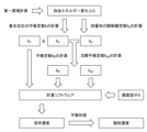
- FIG. 1 is a flow chart of calculating the saturated silica concentration Ce 1 and the dissolved silica concentration C 1 in the prediction method according to the first aspect of the present invention.
- FIG. 2 is a graph showing an example of a prediction curve showing the relationship between the polymerization reaction temperature T and the saturation concentration Ce 1 at pH 7, which can be used in the prediction method according to the first aspect of the present invention.
- FIG. 3 is a graph showing an example of a prediction curve showing the relationship between the polymerization reaction time t, the dissolved silica concentration C1, and the amount of precipitated silica at 100° C. and pH 7 , which can be used in the prediction method according to the first aspect of the present invention. is.
- FIG. 1 is a flow chart of calculating the saturated silica concentration Ce 1 and the dissolved silica concentration C 1 in the prediction method according to the first aspect of the present invention.
- FIG. 2 is a graph showing an example of a prediction curve showing the relationship between the polymerization reaction temperature T and the saturation concentration Ce
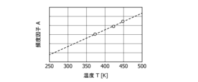
- FIG. 4 is a semi-logarithmic graph showing the prediction curve of the frequency factor A used in fitting to accurately predict the dissolved concentration in the early stage of the reaction, the vertical axis being logarithmic scale. By using the frequency factor A, the experimental values at each temperature can be reproduced at a time point of 5 min.
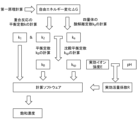
- FIG. 5 is a flow chart of calculating the saturated silica concentration Ce2 and the dissolved silica concentration C2 in the prediction method according to the second aspect of the present invention.
- FIG. 6 is a graph showing an example of a prediction curve showing the relationship between the polymerization reaction temperature T and the saturation concentration Ce 2 at pH 5.5 and pH 7.0, which can be used in the prediction method according to the second aspect of the present invention. .
- FIG. 5 is a flow chart of calculating the saturated silica concentration Ce2 and the dissolved silica concentration C2 in the prediction method according to the second aspect of the present invention.
- FIG. 6 is a graph showing an example of a prediction curve showing the relationship between the poly
- FIG. 7 shows an example of a prediction curve showing the relationship between the polymerization reaction time t, the dissolved silica concentration C2 , and the silica precipitation amount at 150° C. and pH 5.5, which can be used in the prediction method according to the second aspect of the present invention. It is a graph representing.
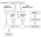
- FIG. 8 is a flow chart for calculating the saturated silica concentration Ce3 and the dissolved silica concentration C3 in the prediction method according to the third aspect of the present invention.
- FIG. 9 is a graph showing changes in the effective reaction coefficient J in the pH range of 7-14.
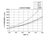
- FIG. 10 is an example of a prediction curve showing the relationship between the polymerization reaction temperature T and the saturation concentration Ce 3 at pH 5.5, pH 7.0, and pH 9.0, which can be used in the prediction method according to the third aspect of the present invention.
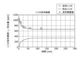
- FIG. 11 shows an example of a prediction curve showing the relationship between the polymerization reaction time t, the dissolved silica concentration C3 , and the silica precipitation amount at 100° C. and pH 9.0, which can be used in the prediction method according to the third aspect of the present invention.
- FIG. 12 is a conceptual diagram illustrating a geothermal power generation system including a silica scale production prediction system according to one embodiment of the present invention.
- the present invention relates to a method for predicting the amount of silica scale produced.
- the method for predicting the amount of silica scale produced includes the following steps. Obtaining the temperature T s (K) at the predicted site where silica scale deposition is to be predicted and/or the time t s (min.) for the fluid containing silicic acid to reach the predicted site; Calculating the amount of silica deposited at the predicted site based on a temperature-dependent silica saturation concentration prediction formula and/or a time-dependent silica dissolved concentration prediction curve.
- the present embodiment relates to a method for predicting the amount of silica scale produced in a plant system in which a fluid containing silicic acid circulates.
- Silicic acid-containing fluids are Si(OH) 4 , Si(OH) 3 O ⁇ , SiO 2 (OH) 2 2 ⁇ , Si 2 O 2 (OH) 5 ⁇ , and/or Si 2 O 3 (OH ) 4 2- refers to fluids containing species containing Si and OH, including but not limited to 2-.
- the plant system may be a plant system that includes pipes and equipment through which a fluid containing silicic acid flows, and is, for example, a plant system that may stop or malfunction due to deposition of silica scale. Examples of plant systems include, but are not limited to, geothermal power generation systems, boiler systems, systems with cooling water piping, and water treatment systems.
- the fluid containing silicic acid may be, for example, water that can contain silicic acid, and examples include, but are not limited to, groundwater, tap water, geothermal water, and wastewater derived therefrom.
- the silicic acid-containing fluid may be geothermal water.
- the fluid is not limited to a liquid, and includes a mixture of water and gas such as steam.
- the amount of silica scale produced in an arbitrary portion of the plant system is predicted based on the temperature T-dependent prediction formula for the saturation concentration of silica Ce1 .
- the silica saturation concentration Ce 1 (saturation concentration) given by the prediction formula refers to silica (including various silica polymers such as monomers and dimers) that can be produced by the condensation polymerization reaction of silicic acid described above. ) dissolves and reaches a saturated solution at a given temperature T (in units of ppm).
- silica scale refers to precipitated silica that cannot be dissolved in a fluid.
- Precipitated silica can usually be a tetramer or a polymer with a higher degree of polymerization, but the degree of polymerization of the polymer is not particularly limited.
- k1 is the reaction equilibrium constant between Si(OH) 4 and SiOSi(OH) 6
- k2 is the reaction equilibrium constant between SiOSi(OH) 6 and (SiO) 3OSi (OH) 10
- k B is the ionization equilibrium constant between SiOSi(OH) 6 and (SiO) 3 Si(OH) 9 O-
- ka is the silicic acid dissociation constant between (SiO) 3 Si(OH) 9 O- and (SiO) 3 OSi(OH) 10 )
- the silica polymerization reaction is a two-step model of a reversible reaction that produces SiOSi(OH) 6 from Si(OH) 4 and an irreversible reaction that produces (SiO) 3OSi (OH) 10 from SiOSi (OH)6.
- Calculations have been made based on In the present invention, instead of this two-step model, by adopting the model of the above formula (1) that further considers the precipitation equilibrium reaction, (SiO) 3 Si(OH) 9 O- Prediction including the dynamics of the represented chemical species becomes possible.
- FIG. 1 is a flow chart for calculating the saturated silica concentration Ce 1 and the dissolved silica concentration C 1 .
- the free energy change in the reaction at each stage of formula (1) Obtain ⁇ G. Also, k 1 and k 2 are obtained from the value of the free energy change ⁇ G.
- the temperature T in the equation for calculating the equilibrium constant of the polymerization reaction is the polymerization reaction temperature.
- the acid dissociation constant ka the following values calculated from the free energy change ⁇ G by quantum chemical calculation and linear fitting correction method can be used.
- pk a p ⁇ G+q
- p and q are constants, and ⁇ G is the value of free energy change in the equilibrium reaction between (SiO) 3 Si(OH) 9 O- and (SiO) 3 OSi(OH) 10 .
- p may range from 0.19 to 0.24 and q may range from -56 to -51.
- p may be between 0.21 and 0.22 and q may be between -54 and -52.
- a 1 and b 1 are constants and are values obtained by the calculation described in the flowchart above.
- T(K) represents the polymerization reaction temperature.
- the temperature range for T may be about 250K to 500K. More specifically, a 1 may be from 18 to 32 and b 1 from 0.005 to 0.010. Preferably, a 1 is 20-30 and b 1 may be 0.006-0.009.
- FIG. 2 is an example of Equation (2) representing a prediction curve for the silica saturation concentration Ce1 .
- the prediction formula according to the present invention is indicated by a solid line. This prediction formula makes it possible to calculate the temperature T dependence of the silica saturation concentration Ce1 .
- the temperature T is the polymerization reaction temperature (unit: K) in the three-stage precipitation equilibrium reaction model represented by the formula (1).
- the temperature T s at a predetermined prediction site where the scale adhesion amount of the actual plant system should be predicted is used as the polymerization temperature, and the prediction calculation is performed. can be used.
- the temperature T s at the predicted site may be, for example, the temperature of the fluid, which may contain silica, at the predicted site of the plant system.
- the prediction method includes the following steps a) to d). a) Step of obtaining temperature T s (K) at the predicted site where silica scale adhesion should be predicted b) Step of calculating silica saturation concentration Ce 1 at the predicted site from temperature T s and prediction formula (2) c ) Obtaining the total silica concentration C t in the fluid containing silicic acid d) Calculating the silica loading based on the total silica concentration C t and the silica saturation concentration Ce 1
- the predicted site where silica scale deposition should be predicted is a site that comes into contact with a fluid containing silicic acid in a plant system that implements the prediction method according to the present embodiment, and where silica scale deposition is expected to occur.
- a fluid containing silicic acid in a plant system that implements the prediction method according to the present embodiment, and where silica scale deposition is expected to occur.
- This is a possible part.
- it may be turbine blades, turbine members such as rotors, piping, heat exchangers, etc., but is not limited to these.
- the method of obtaining the temperature T s (K) is not particularly limited, but for example, a temperature measuring device such as a temperature sensor installed at a specific location actually measures the temperature of the fluid or equipment at the predicted site, and if necessary
- the fluid temperature can be calculated from the measured temperature of the device to be Ts .
- Step b) can be performed by an arithmetic device capable of performing calculations according to prediction formula (2).
- the arithmetic device may be, for example, a computer in which a specific arithmetic program is installed, but is not particularly limited.
- the total silica concentration Ct is the total concentration of silica present in the fluid supplied to the plant system embodying the present invention.
- the total silica concentration Ct is the weight percent concentration (ppm) in the fluid of the silica monomer (Si(OH) 4 ) calculated based on the amount of all Si atoms present in the fluid. . Of this amount, it is considered that the amount exceeding the silica saturation concentration Ce precipitates and adheres as silica scale.
- the total silica concentration Ct can be calculated, for example, as follows. First, the geothermal water pumped from the production well is analyzed to obtain the mass or molar amount of Si atoms in the geothermal water.
- the weight percent concentration of the silica monomer in the geothermal water is calculated.
- the portion of the total silica concentration Ct exceeding the saturation concentration precipitates as silica scale.
- the amount of silica scale deposited can be obtained by calculating the difference between the total silica concentration Ct obtained in step c) and the saturated silica concentration Ce 1 using a computing device.
- the computing device may be a computer in which a specific computing program is installed, as in step b), but is not particularly limited.
- the amount of silica scale produced in an arbitrary portion of the plant system is also predicted based on the prediction curve of the time-dependent dissolved silica concentration C1 .
- a prediction curve showing the relationship between the time t and the dissolved silica concentration C1 is obtained by calculation, and the silica adhesion amount is calculated from the prediction curve.
- the dissolved silica concentration C1 at time t is the concentration of silica dissolved in the fluid at time t (min) when the polymerization start point is zero.
- the silica concentration here refers to the amount of silica monomer (Si(OH) 4 ) calculated based on the amount of Si atoms dissolved in the fluid in the same manner as explained for the total silica concentration Ct above. , is the weight percent concentration (ppm) in the fluid.
- the initial silica concentration C i is also expressed in weight percent concentration (ppm) in the fluid of silica monomer (Si(OH) 4 ) calculated based on the amount of Si atoms dissolved in the fluid.
- the time t is the time (min) when the point at which Si(OH) 4 is dissolved in the fluid is set to 0 in the three-stage precipitation equilibrium reaction model represented by Equation (1).
- the point of time recognized as the start of the polymerization reaction in the actual plant system can be used as 0 for the prediction calculation. For example, in a geothermal power generation system, zero can be the point in time when geothermal water is pumped up from a production well.
- the prediction curve acquisition method includes the following steps i) to iii). i) Step of obtaining the initial silica concentration C i ii) Calculate k 1 , k 2 , k B , ka in the three-step precipitation equilibrium reaction model of formula (1), and determine the initial silica concentrations C i and k 1 , calculating a predicted value for the dissolved silica concentration C 1 from k 2 , k B , and ka ; iii) Plotting the dissolved silica concentration C1 against time t and performing curve fitting based on the plotted results to obtain a predicted curve of the dissolved silica concentration C1 .
- Step i) is the step of obtaining the initial silica concentration C i .
- the initial silica concentration C i can be assumed to be computationally equal to the total silica concentration C t . Therefore, the initial silica concentration C i can be obtained in the same manner as the total silica concentration C t by the method described above.
- k 1 , k 2 , k B , ka are calculated according to the flow chart of FIG.
- a predicted value of the dissolved silica concentration C 1 is calculated from the initial silica concentration C i and k 1 , k 2 , k B , and ka .
- the predicted value of the dissolved silica concentration C1 is preferably obtained at a plurality of different times t, and can be calculated at, for example, 10 or more points, preferably 50 or more points, and more preferably 100 or more different times t. This makes it possible to obtain a predicted value for the dissolved concentration C1 from the start of the reaction to the desired point in time.
- step iii) the dissolved silica concentration C1 is plotted against time t, and a predicted curve of the dissolved silica concentration C1 is obtained based on the plotted results.
- FIG. 3 is an example of a predicted curve of the dissolved silica concentration C1 obtained in step iii), which is obtained at a temperature of 100° C. and pH 7 when the initial concentration is about 1100 ppm.
- the solid line represents the dissolved silica concentration C 1 (unit: ppm), and the dashed-dotted line represents the amount of silica precipitation (unit: ppm).
- the silica precipitation amount refers to the mass of silica tetramer produced from the fluid per unit volume (1 L).
- the mass of silica tetramer produced from the fluid per unit volume is the mass of silica tetramer produced from the fluid per unit mass (1 kg) can be approximated as Therefore, the sum of the dissolved silica concentration C1 and the amount of precipitated silica is the initial silica concentration C1 .
- a frequency factor A is required to fit the polymerization temperature T to the expected value of the dissolved silica concentration C1 at the initial stage of the reaction.
- the initial stage of the reaction refers to the stage of about 5 to 10 minutes after the start of the reaction, although it varies depending on the reactor, conditions, and the like.
- the relationship between the polymerization temperature T and the frequency factor A is represented by the following formula (3).
- A m[exp(nT)] (3)
- m and n are constants and are values obtained by the calculations described in the flowchart above.
- T(K) represents the polymerization reaction temperature.
- the temperature range for T is about 250K to 500K. More specifically, m may be from 2.0 to 3.1 and n may be from 0.083 to 0.085. Preferably, m is between 2.3 and 2.8 and n may be between 0.0835 and 0.0845.
- FIG. 4 is a semilogarithmic graph showing the prediction curve of frequency factor A, where the vertical axis is a logarithmic scale.
- the prediction method includes the following steps A) to D).
- A) A step of obtaining the time t s (min.) for the fluid containing silicic acid to reach the predicted site B) From the predicted curve of the temperature time t s and the dissolved silica concentration C 1 , the silica at the predicted site C) obtaining the total silica concentration Ct in the fluid containing silicic acid; D) calculating the amount of silica deposition at time t based on the total silica concentration Ct and the dissolved silica concentration C1 .
- the time ts can be obtained by simulation based on the plant system operating conditions.
- the time t s (min.) may be the time required for geothermal water pumped from a production well to reach a predetermined predicted site.
- Step B) can be performed by a computing device capable of performing the computation of calculating the dissolved silica concentration C1 from the predicted curve.
- Steps C) and D) can be carried out in the same manner as the previous steps c) and d).
- the total silica concentration C t according to this embodiment is equal to the initial silica concentration C i . Therefore, the initial silica concentration Ci used to derive the dissolved silica concentration C1 can be calculated as the total silica concentration Ct .
- the silica saturation concentration Ce 1 and / Or, the dissolved silica concentration C1 can be predicted, and the amount of silica scale produced can be predicted that can cope with complicated conditions in a short time and on a low budget.
- the amount of silica scale produced in an arbitrary part of the plant system is predicted based on a prediction formula for the silica saturation concentration Ce 2 depending on the temperature T and pH.
- the second aspect provides a prediction formula that is particularly useful when the pH of the fluid in which silicic acid is dissolved is 0 or more and less than 7. Therefore, the prediction formula according to this aspect may also be referred to as the prediction formula for the acidic region.
- the silica saturation concentration Ce 2 given by the prediction formula of this embodiment is the weight percent concentration of the solution in which silica that can be produced by the condensation polymerization reaction of silicic acid is dissolved and reaches a saturated solution at a predetermined temperature T and pH. (The unit is ppm). In other words, it refers to the maximum concentration at which silica can be dissolved at a given temperature T and pH.
- the definitions of silicic acid, silica, and silica scale are the same as in the first aspect.
- a 2 may range from 16 to 36 and b 2 may range from 0.003 to 0.015.
- a 2 may be from 18 to 35 and b 2 from 0.005 to 0.012.
- a 2 may be from 20 to 33 and b 2 from 0.006 to 0.010.
- the temperature range for T may be about 250K to 500K.
- R can be calculated based on the following formula, and is a coefficient that determines the influence of the pH in the acidic region (pH 0 or more and less than 7) on the silica saturation concentration.
- ⁇ logR A R Z 2 ⁇ E/(1+B R cE) ⁇ (5)
- a R and B R are values calculated from the temperature T of the silica polymerization reaction system and the dielectric constant ⁇ of water, which is the silica polymerization reaction solvent, based on the Debye-Huckel theory,
- the charge number Z is 1 or 2
- the effective diameter coefficient c is 4
- E is the effective ionic strength represented by the following formula (6), and can be represented by the following formula.
- E ⁇ I+(hydrogen ion concentration) ⁇ /[1+B R c[I+(hydrogen ion concentration)] (6) (In formula (6), I is the solute ionic strength) ⁇
- a R and B R can be represented by the following formulas.
- a R 1.825*10 6 ( ⁇ T) ⁇ 3/2
- T(K) represents the polymerization reaction temperature.
- the charge number Z is 1 or 2.
- the amount of silica is 1. 2 in the case of divalent ions of isomers and dimers (SiO 2 (OH) 2 2- S 2 O 2 (OH) 6 2- ).
- the effective diameter factor c is a constant 4 in silica polymerization reactions.
- the hydrogen ion concentration can be calculated from a predetermined pH of 0 or more and less than 7. For example, when the pH is 5.5, it is 10 ⁇ (-5.5).
- FIG. 6 is an example of Equation (4) representing a prediction curve for silica saturation concentration Ce 2 .
- FIG. 6 shows a prediction curve at pH 5.5 and a prediction curve at pH 7.0 (in the first aspect) based on the prediction formula according to the second aspect of the present invention.
- different pH yields different prediction curves.
- the prediction formula according to the second aspect can be derived by the above-described method at each pH in the range of pH 0 or more and less than 7, and a prediction curve can be drawn.
- the prediction curve of the comparative example was obtained based on empirical rules according to the method disclosed in Non-Patent Document 1, but the pH was not strictly considered, and the prediction curve was different from that of the present embodiment. ing.
- the prediction formula according to the second aspect makes it possible to calculate the temperature T and pH dependence of the silica saturation concentration Ce 2 .
- the temperature T is the polymerization reaction temperature (unit: K) in the three-stage precipitation equilibrium reaction model represented by the formula (1).
- the temperature T s at a predetermined prediction site where the scale adhesion amount of the actual plant system should be predicted is used as the polymerization temperature.
- the pH can be used to calculate the effective activity coefficient, R, and used in predictive calculations.
- the temperature T s at the predicted site can be determined in the same manner as in the first aspect.
- the pH at the predicted site may be the pH of the fluid, which may contain silica, at the predicted site of the plant system.
- the prediction method includes the following steps a) to d). a) Step of acquiring temperature T s (K) and pH at the prediction site where silica scale adhesion should be predicted b) From temperature T s , pH and prediction formula (4), silica saturation concentration Ce 2 at the prediction site c) obtaining the total silica concentration C t in the fluid containing silicic acid d) calculating the silica loading based on the total silica concentration C t and the silica saturation concentration Ce 2
- the method for predicting the amount of silica scale deposited can be carried out in the same manner as in the first aspect except that in step a) the pH at the predicted site is obtained and in step b) the calculation is performed using the prediction formula (4). can.
- the pH value at the predicted site can be measured using a normal pH meter, or can be calculated by a method such as simulation.
- the method for predicting the silica scale deposit amount according to the present embodiment, it is possible to predict the deposit amount according to the acidic pH conditions of the fluid in which silica scale is a problem. Then, more accurate prediction becomes possible as compared with the conventional technology.
- the generation amount of silica scale at an arbitrary portion of the plant system is also predicted based on the prediction curve of the dissolved silica concentration C2 depending on time.
- a prediction curve showing the relationship between the time t and the dissolved silica concentration C2 is obtained by calculation, and the silica adhesion amount is calculated from the prediction curve.
- a method for obtaining a time-dependent silica dissolved silica concentration prediction curve C2 includes the following steps i) to iii).
- the method of obtaining the predicted curve of the dissolved silica concentration C2 is as follows: In calculating the predicted value of the dissolved silica concentration C2 in step ii), the pH condition is taken into consideration, and the effective activity of the prediction formula (4) is It may be the same as the first embodiment, except that the volume factor R needs to be calculated. Also, the method of calculating the frequency factor A and the preferable values of the constants m and n for determining the frequency factor can be the same as in the first mode.
- FIG. 7 is an example of a predicted curve for the dissolved silica concentration C2 obtained by steps i) to iii) of the second embodiment, obtained at a temperature of 150° C. and a pH of 5.5 when the initial concentration is about 1300 ppm. 5 is the prediction curve.
- the solid line represents the dissolved silica concentration C (in units of ppm)
- the dashed-dotted line represents the silica precipitation amount (in units of ppm).
- the prediction method may be the same as steps A) to D) of the first aspect, except that the prediction curve for the dissolved silica concentration C2 is used for calculation.
- the temperature and pH at the desired site do not require empirical values such as experimental values and actual measured values. It is possible to predict the saturated silica concentration Ce2 and/or the dissolved silica concentration C2 , and to predict the amount of silica scale produced that can respond to complex conditions in a short time and on a low budget. In particular, it is possible to predict the amount of silica scale produced in consideration of the polymerization reaction of silica at pH in the acidic range.
- the amount of silica scale produced in an arbitrary part of the plant system is predicted based on the prediction formula for the saturated concentration of silica Ce 3 depending on the temperature T and pH. .
- the third aspect provides a prediction formula that is particularly useful when the pH of the fluid in which silicic acid is dissolved is greater than 7 and equal to or less than 14. Therefore, the prediction formula according to this aspect is also referred to as a prediction formula for basic regions.
- the definition of the silica saturation concentration Ce 3 given by the prediction formula of the third aspect is the same as in the second aspect, and the definitions of silicic acid, silica, and silica scale are the same as in the first aspect.
- FIG. 8 is a flow chart for calculating the saturated silica concentration Ce3 and the dissolved silica concentration C3 . Also in the prediction formula for the basic region, a calculation formula is derived based on the three-step precipitation equilibrium reaction model of silica polymerization represented by the above formula (1).
- J is an effective reaction coefficient, which is a value calculated based on the existing fractions of silica monomer ions and silica dimer ions.
- a 3 may be 6 to 34 and b 3 may be 0.005 to 0.015.
- a 3 is 8 to 32 and b 3 may be 0.005 to 0.015.
- a 3 may be 10-30, b 3 may be 0.006-0.009, and the temperature range of T may be about 250K to 500K.
- J can be calculated based on the following formula, and is a coefficient that determines the effect of the pH in the basic region on the silica saturation concentration. Based on the inventors' discovery that in the basic region, ions do not directly participate in the silica polymerization reaction, but are determined by the fraction of silica present in the non-ionized molecular state.
- the effective reaction coefficient J can be expressed by the following formula (8).
- X is the total amount of silica (molar amount, 100%)
- Xi 1 and Xi 2 are the existing fractions of silica monomer ions and silica dimer ions (molar fraction %)
- Silica monomer ions are Si(OH) 3 O ⁇
- silica dimer ions are Si 2 (OH) 7 O ⁇ .
- the acid dissociation constant k aj is an equilibrium constant when considering a dissociation reaction in which protons (hydrogen ions) are released from silica monomer, silica dimer and silica tetramer molecules.
- FIG. 10 is an example of Equation (7) representing a prediction curve for the silica saturation concentration Ce 3 .
- Fig. 2 shows a prediction curve at pH 9.0 and a prediction curve (in the first aspect) at pH 7.0 based on the prediction formula according to the third aspect of the present invention;
- the prediction formula according to the third aspect can be derived by the above method at each pH in the range from pH 7 to 4, and a prediction curve can be drawn.
- a prediction curve at pH 5.5 based on the prediction formula according to the second aspect is also shown in the graph.
- different pH yields different prediction curves.
- the prediction curve of the comparative example was obtained based on empirical rules according to the method disclosed in Non-Patent Document 1, but the pH was not strictly considered, and the prediction curve was different from that of the present embodiment. ing.
- the prediction formula according to the third aspect makes it possible to calculate the temperature T and pH dependence of the silica saturation concentration Ce3 .
- the temperature T is the polymerization reaction temperature (unit: K) in the three-stage precipitation equilibrium reaction model represented by the formula (1).
- each step of predicting the silica scale adhesion amount is the same as the second aspect except that the silica saturation concentration Ce 3 is calculated based on the formula (7).
- the method for predicting the amount of silica scale deposited according to the third aspect it is possible to predict the amount of deposited silica scale according to the basic pH conditions of the fluid in which silica scale is a problem. Accurate prediction of adhesion amount becomes possible.
- the third aspect similarly to the second aspect, it is possible to predict the amount of silica scale generated in any part of the plant system based on the time-dependent prediction curve of the dissolved silica concentration C3 .
- a prediction curve showing the relationship between the time t and the dissolved silica concentration C3 is obtained by calculation, and the silica adhesion amount is calculated from the prediction curve.
- Each step of the method for obtaining a prediction curve for the time-dependent dissolved silica concentration C3 of silica in step ii) of the second aspect is k 1 , k 2 , k 2 , Calculate k B , ka , calculate the effective reaction coefficient J, and calculate the predicted value of the dissolved silica concentration C 3 from the initial silica concentration C i and k 1 , k 2 , k B , ka , J
- the method of calculating the frequency factor A and the preferable values of the constants m and n for determining the frequency factor can be the same as in the first mode.
- FIG. 11 is an example of a prediction curve of the dissolved silica concentration C3 obtained by steps i) to iii) similar to the second embodiment, obtained when the initial concentration is about 1050 ppm, at a temperature of 100 ° C., Prediction curve at pH9.
- the solid line represents the dissolved silica concentration C 3 (unit: ppm)
- the dashed-dotted line represents the silica precipitation amount (unit: ppm).
- the temperature and pH at the desired site do not require empirical values such as experimental values and actual measured values. It is possible to predict the saturated silica concentration Ce3 and/or the dissolved silica concentration C3 , and to predict the amount of silica scale produced that can cope with complicated conditions in a short time and on a low budget. In particular, it is possible to predict the amount of silica scale produced in consideration of the polymerization reaction of silica at pH in the basic range.
- the present invention is a silica scale deposition amount prediction system including the following. Apparatus for acquiring temperature T s (K) at a predicted site where silica scale deposition should be predicted and/or time t s (min.) for a fluid containing silicic acid to reach the predicted site Temperature dependent Based on the prediction formula of the saturated silica concentration Ce 1 , Ce 2 , or Ce 3 and/or the prediction curve of the dissolved silica concentration C 1 , C 2 , or C 3 depending on time, the amount of silica attached at the predicted site A device that calculates
- the prediction formula of the silica saturation concentration Ce 1 , Ce 2 , or Ce 3 and the prediction curve of the dissolved silica concentration C 1 , C 2 , or C 3 with respect to time are the first aspect of the first embodiment can be obtained in the same manner as in the third embodiment, and a description thereof will be omitted.
- a device for obtaining temperature T s (K) and/or time t s (min.), a device for calculating the silica deposition amount, and a device for measuring pH also perform each step in each aspect of the first embodiment. can be selected from options similar to those specifically listed for the device.
- the silica scale generation amount prediction system according to this embodiment can be incorporated into various plant systems, and it is possible to predict the silica scale generation amount according to the conditions of the plant system.
- the present invention relates to a geothermal power generation system, a gas-liquid separator that separates the geothermal fluid pumped up from the production well into gas and liquid components; a turbine disposed downstream of the gas-liquid separator and configured to be rotatable by gas components separated by the gas-liquid separator; a pipe for delivering the liquid component separated by the gas-liquid separator to a reinjection well; and a prediction system for the silica scale production amount of the second embodiment.
- FIG. 12 is a conceptual diagram illustrating a geothermal power generation system according to the third embodiment.
- the geothermal power generation system 1 includes a production well 6, a gas-liquid separator 2, a turbine 3, a generator 4, a condenser 5, a reduction well 7, and a silica scale generation amount prediction system.
- the silica scale production amount prediction system is the system described in the second embodiment, and is a system capable of implementing the prediction method described in the first embodiment.
- Production wells 6 are wells that lead into the ground hot water, steam, or mixtures thereof (hereafter referred to as geothermal fluids) in geothermal reservoirs in the ground.
- geothermal fluids The geothermal fluid drawn from the production well 6 is separated by the gas-liquid separator 2 into steam, which is a gas component, and hot water, which is a liquid component.
- the separated steam is directed to turbine 3 and used to rotate turbine 3 to produce electricity in generator 4 .
- the steam that has passed through the turbine 3 is cooled by the condenser 5 and guided to the reinjection well 7 through a pipe (not shown).
- the hot water separated by the gas-liquid separator 2 is cooled and led to the reinjection well 7 .
- the site where silica scale deposition should be predicted in the plant system is not particularly limited, and may be any site where geothermal fluid may adhere.
- the predicted part may be the turbine member or the like exemplified in the first embodiment, but is not limited to these.
- the predicted site may be a member not specifically shown in FIG.
- the number of predicted parts may be one in the plant system, or two or more. Theoretically, the upper limit of the number of predicted parts is not limited.
- the geothermal power generation system it is possible to accurately predict the amount of silica scale adhered, and it is possible to minimize the shutdown of the system and perform maintenance at an appropriate time. It is possible to generate power efficiently and effectively. In particular, it is possible to predict the amount of silica scale deposition by also considering the pH of the geothermal fluid flowing through the geothermal power generation system.
- Formula (1) was used as a reaction model for the silica polymerization reaction in hot water, and a model corresponding to the silica polymerization reaction was created using the reaction module of calculation software (COMSOL Multiphysics (registered trademark) modeling software).
- the acid dissociation constant is calculated as follows based on the definition of the acid dissociation constant. Since protons do not have electrons, G(H + ) cannot be calculated, so in the comparative example, ⁇ G was calculated by approximately substituting G(H 3 O + ). On the other hand, the experimental value is the literature value of the acid dissociation constant of the monomer.
- the ionization equilibrium constant k B and the precipitation equilibrium constant k sp could be calculated as follows.
- a prediction curve for the dissolved silica concentration C1 was obtained by substituting the various parameters and frequency factor A described above into the software. From the obtained prediction curve of the dissolved silica concentration C1 , the saturated concentration was estimated at the equilibrium state.
- the dissolved experimental value indicates the saturation concentration of silica obtained from the result of a hydrothermal synthesis experiment simulating the fluid of a power generation facility using a small-scale experimental apparatus.
- a comparative example shows the saturation concentration of silica predicted by the conventional method. Since the conventional method cannot obtain time-dependent calculation results, only one point is plotted.
- the prediction formula is represented by the previous formula (2).
- the predicted value of the saturated concentration (Example) was compared with the calculated result of the comparative example and the experimental value described above, and the established saturated concentration prediction formula was verified.
- the solid line is the calculation result of the example
- the dashed line is the calculation result of the comparative example
- the white circles are the experimental values. From FIG. 2, it was shown that the predicted values of the example by this method were well matched to the experimental values, and accurate prediction could be made.
- frequency factor A was plotted at temperature conditions of 373.15K, 423.15K and 448.15K. The results are shown in FIG. From FIG. 4, equation (3) was obtained, establishing an equation showing the temperature dependence of the frequency factor A.
- FIG. 1 An example of the predicted curve of the dissolved silica concentration C2 at 150° C. (423.15 K) and pH 5.5 is shown in FIG.
- the dissolution experiments were the same as the dissolution experiments according to the first aspect, except that they were performed at pH 5.5.
- a variance analysis was performed on the obtained saturation curve to establish a prediction formula for the silica saturation concentration.
- the prediction formula is represented by the previous formula (4). The plot of the dissolved experimental values fitted well to the predicted value of pH 5.5 by this method, indicating that an accurate prediction could be made.
- FIG. 11 shows an example of a predicted curve for the dissolved silica concentration C3 at 100° C. (373.15 K) and pH 9.0.
- the dissolution experimental values are the same as the dissolution experiments according to the first aspect, except that they were carried out at pH 9.0.
- a variance analysis was performed on the obtained saturation curve to establish a prediction formula for the silica saturation concentration.
- For the frequency factor A the same value as in the first aspect was used.
- the prediction formula is represented by the previous formula (7).
- the plot of the dissolved experimental values fitted well to the predicted value of pH 9.0 by this method, indicating that an accurate prediction could be made.
Landscapes
- Engineering & Computer Science (AREA)
- Life Sciences & Earth Sciences (AREA)
- Chemical & Material Sciences (AREA)
- Theoretical Computer Science (AREA)
- Computing Systems (AREA)
- Combustion & Propulsion (AREA)
- Biochemistry (AREA)
- Mechanical Engineering (AREA)
- Analytical Chemistry (AREA)
- General Engineering & Computer Science (AREA)
- General Health & Medical Sciences (AREA)
- General Physics & Mathematics (AREA)
- Immunology (AREA)
- Pathology (AREA)
- Environmental & Geological Engineering (AREA)
- Physics & Mathematics (AREA)
- Sustainable Energy (AREA)
- Health & Medical Sciences (AREA)
- Bioinformatics & Computational Biology (AREA)
- Sustainable Development (AREA)
- Bioinformatics & Cheminformatics (AREA)
- Ecology (AREA)
- Biodiversity & Conservation Biology (AREA)
- Environmental Sciences (AREA)
- Hydrology & Water Resources (AREA)
- Water Supply & Treatment (AREA)
- Organic Chemistry (AREA)
- Management, Administration, Business Operations System, And Electronic Commerce (AREA)
Abstract
Description
[1] シリカスケールの付着を予測すべき予測部位における温度Ts(K)、及び/またはケイ酸を含む流体が、前記予測部位に到達するまでの時間ts(min.)を取得する工程と、
温度に依存したシリカ飽和濃度の予測式、及び/または時間に依存したシリカ溶存濃度の予測曲線に基づいて、前記予測部位におけるシリカ付着量を計算する工程と
を含み、
前記シリカ飽和濃度の予測式及び前記シリカ溶存濃度の予測曲線が、以下の式(1)で表される3段階沈殿平衡反応モデル

(式(1)中、
k1は、Si(OH)4とSiOSi(OH)6との間の反応平衡定数であり、
k2は、SiOSi(OH)6と(SiO)3OSi(OH)10との間の反応平衡定数であり、
kBは、SiOSi(OH)6と(SiO)3Si(OH)9O-との間のイオン化平衡定数であり、
kaは、(SiO)3Si(OH)9O-と(SiO)3OSi(OH)10との間のシリカ酸解離定数である)
における、k1、k2、kB、kaに基づいて得られる、シリカスケール生成量の予測方法。
[2] 前記シリカ酸解離定数kaが、(SiO)3Si(OH)9O-と(SiO)3OSi(OH)10との平衡反応における自由エネルギー変化ΔGに基づき、量子化学計算及び線形フィッティング補正法により得られる、[1]に記載の方法。
[3] 前記シリカ酸解離定数kaと、前記自由エネルギー変化ΔGの関係が、
pka=pΔG+q
(式中、p、qは定数である)
で表される、[2に記載の方法。
[4] pが、0.19~0.24であり、qが、-56~-51である、[3に記載の方法。
[5] 前記シリカ溶存濃度Cの予測曲線が、シリカ初期濃度Ciと式(1)に基づいて第1原理計算により得られた2以上の異なる時間時点に対するシリカ溶存濃度のプロットを、フィッティングすることにより得られ、
反応初期のフィッティングの補正に用いる頻度因子Aが、
A=m[exp(nT)] (3)
(式(3)中、m、nは定数であり、k1、k2、kB、kaに基づいて計算される)
で表される、[1]に記載の方法。
[6] mが、2.0~3.1であり、nが、0.083~0.085である、[5]に記載の方法。
[7] 前記シリカ飽和濃度Ceの予測式が、温度Tにおけるシリカ飽和濃度Ce1:
Ce1=a1[exp(b1T)] (2)
(式(2)中、
a1、b1は、k1、k2、kB、kaに基づいて計算される定数であり、
Tは重合反応温度を表す)
で表される、[1]に記載の方法。
[8] a1が、18~32であり、b1が、0.005~0.010である、[7]に記載の方法。
[9]
前記シリカ飽和濃度Ce2の予測式が、温度T、pHが0以上であって7未満におけるシリカ飽和濃度Ce2:
Ce2=R{a2[exp(b2T)]} (4)
(式(4)中、
a2、b2は、k1、k2、kB、kaに基づいて計算される定数であり、
Rは、pHに基づいて計算される実効活量係数であり、
Tは重合反応温度を表す)
で表される、[1]に記載の方法。
[10] 前記実効活量係数Rの計算式が、
-logR= ARZ2{E/(1+BRcE)} (5)
{式(5)中、
AR=1.825*106(εT)-3/2、
BR=50.3*(εT)-1/2
で表され、
電荷数Zは、1または2から選択される定数であり、有効径係数cは4であり、
Eが、以下の式(6)で表される実効イオン強度
E={I+(水素イオン濃度)}/[1+BRc[I+(水素イオン濃度)] (6)
(式(6)中、Iは溶質イオン強度である)
である}
で表される、[9]に記載の方法。
[11] a2が、16~36であり、b2が、0.003~0.015である、[9]に記載の方法。
[12] 前記シリカ飽和濃度Ce3の予測式が、温度T、pHが7より大きく、14以下におけるシリカ飽和濃度Ce3:
Ce3=(1-J){a3[exp(b3T)]} (7)
(式(7)中、
a3、b3は、k1、k2、kB、kaに基づいて計算される定数であり、
Jは、シリカ単量体イオンとシリカ2量体イオンの存在分率に基づいて計算される実効反応係数であり、
Tは重合反応温度を表す)
で表される、[1]に記載の方法。
[13] 前記実効反応係数Jの計算式が、
J=(X-Xi1-Xi2)/X (8)
(式(8)中、
Xは、シリカの総量であり、
Xi1は、酸解離定数kajから計算されるシリカ単量体イオンの存在分率であり、
Xi2、酸解離定数kajから計算されるシリカ2量体イオンの存在分率である)
で表される、[12]に記載の方法。
[14] a3が、6~34であり、b3が、0.005~0.015である、[12に記載の方法。
[15] 前記ケイ酸を含む流体中の総シリカ濃度Ctを取得する工程と、
前記総シリカ濃度Ctと、シリカ飽和濃度に基づいてシリカ付着量を計算する工程と
により、前記シリカ付着量が予測される、[1]に記載の方法。
[16] 前記シリカ溶存濃度の予測曲線に基づいてシリカ付着量を計算する工程により、前記シリカ付着量が予測される、[1]に記載の方法。
[17] シリカスケールの付着を予測すべき予測部位における温度Ts(K)、及び/またはケイ酸を含む流体が、前記予測部位に到達するまでの時間ts(min.)を取得する装置と、
温度に依存したシリカ飽和濃度の予測式、及び/または時間に依存したシリカ溶存濃度の予測曲線に基づいて、前記予測部位におけるシリカ付着量を計算する装置と
を含み、
前記シリカ飽和濃度の予測式及び前記シリカ溶存濃度の予測曲線が、以下の式(1)で表される3段階沈殿平衡反応モデル

(式(1)中、
k1は、Si(OH)4とSiOSi(OH)6との間の反応平衡定数であり、
k2は、SiOSi(OH)6と(SiO)3OSi(OH)10との間の反応平衡定数であり、
kBは、SiOSi(OH)6と(SiO)3Si(OH)9O-との間のイオン化平衡定数であり、
kaは、(SiO)3Si(OH)9O-と(SiO)3OSi(OH)10との間のシリカ酸解離定数である)
における、k1、k2、kB、kaに基づいて得られる、シリカスケール生成量の予測システム。
[18] 生産井からくみ上げた地熱流体を気体成分と液体成分に分離する気液分離器と、
前記気液分離器の後段に配置され、当該気液分離器で分離された気体成分により回転可能に構成されたタービンと、
前記気液分離器で分離された液体成分を還元井に配送する配管と、
[17]に記載のシリカスケール生成量の予測システムと
を備える地熱発電システム。
本発明は、第1実施形態によれば、シリカスケール生成量の予測方法に関する。シリカスケール生成量の予測方法は、以下の工程を含む。
シリカスケールの付着を予測すべき予測部位における温度Ts(K)、及び/またはケイ酸を含む流体が、前記予測部位に到達するまでの時間ts(min.)を取得する工程と、
温度に依存したシリカ飽和濃度の予測式、及び/または時間に依存したシリカ溶存濃度の予測曲線に基づいて、前記予測部位におけるシリカ付着量を計算する工程
本実施形態に係る方法の第1態様においては、温度Tに依存したシリカの飽和濃度Ce1の予測式に基づき、プラントシステムの任意の部位におけるシリカスケールの生成量を予測する。第1態様では、pHが7の場合の予測式を提供する。ここで、予測式が与えるシリカ飽和濃度Ce1(saturation concentration)とは、先に述べたケイ酸の縮合重合反応により生成されうるシリカ(単量体及び二量体以上の各種シリカ重合体を含む)が溶解して、所定の温度Tにおいて飽和溶液に達する溶液の重量%濃度(単位はppm)をいうものとする。言い換えれば、所定の温度Tにおいて、シリカ(単量体及び二量体以上の各種シリカ重合体を含む)の溶解し得る最大濃度をいう。また、シリカスケールとは、流体に溶解することができず、析出したシリカをいうものとする。析出するシリカは通常、四量体またはそれより重合度の高い多量体でありうるが、多量体の重合度は特には限定されない。

(式(1)中、
k1は、Si(OH)4とSiOSi(OH)6との間の反応平衡定数であり、
k2は、SiOSi(OH)6と(SiO)3OSi(OH)10との間の反応平衡定数であり、
kBは、SiOSi(OH)6と(SiO)3Si(OH)9O-との間のイオン化平衡定数であり、
kaは、(SiO)3Si(OH)9O-と(SiO)3OSi(OH)10との間のシリカ酸解離定数である)
pka=pΔG+q
式中、p、qは定数であり、ΔGは、(SiO)3Si(OH)9O-と(SiO)3OSi(OH)10との平衡反応における自由エネルギー変化の値である。より具体的には、pが、0.19~0.24であり、qが、-56~-51であってよい。好ましくは、pが、0.21~0.22であり、qが、-54~-52であってよい。
Ce1=a1[exp(b1T)] (2)
式(2)中、a1、b1は定数であり、上記フローチャートに記載の計算により得られる値である。T(K)は重合反応温度を表す。Tの温度範囲は、約250Kから500Kであってよい。より具体的には、a1が、18~32であり、b1が、0.005~0.010であってよい。好ましくは、a1が、20~30であり、b1が、0.006~0.009であってよい。
a)シリカスケールの付着を予測すべき予測部位における温度Ts(K)を取得する工程
b)温度Tsと予測式(2)から、前記予測部位におけるシリカ飽和濃度Ce1を計算する工程
c)ケイ酸を含む流体中の総シリカ濃度Ctを取得する工程
d)総シリカ濃度Ctと、シリカ飽和濃度Ce1に基づいてシリカ付着量を計算する工程
i)シリカ初期濃度Ciを取得する工程
ii)式(1)の3段階沈殿平衡反応モデルにおける、k1、k2、kB、kaを計算し、シリカ初期濃度Ciとk1、k2、kB、kaから、シリカ溶存濃度C1の予測値を計算する工程と、
iii)時間tに対する、シリカ溶存濃度C1をプロットし、プロット結果に基づいてカーブフィッティングすることにより、シリカ溶存濃度C1の予測曲線を得る工程
A=m[exp(nT)] (3)
式(3)中、m、nは定数であり、上記フローチャートに記載の計算により得られる値である。T(K)は重合反応温度を表す。Tの温度範囲は、約250Kから500Kである。より具体的には、mが、2.0~3.1であり、nが、0.083~0.085であってよい。好ましくは、mが、2.3~2.8であり、nが、0.0835~0.0845であってよい。
A)ケイ酸を含む流体が、前記予測部位に到達するまでの時間ts(min.)を取得する工程
B)温度時間tsとシリカ溶存濃度C1の予測曲線から、前記予測部位におけるシリカ溶存濃度Cを得る工程
C)ケイ酸を含む流体中の総シリカ濃度Ctを取得する工程
D)総シリカ濃度Ctと、シリカ溶存濃度C1に基づいて、時間tにおけるシリカ付着量を計算する工程
次に、本実施形態に係る方法の第2態様においては、温度T及びpHに依存したシリカの飽和濃度Ce2の予測式に基づき、プラントシステムの任意の部位におけるシリカスケールの生成量を予測する。第2態様では、ケイ酸が溶解している流体のpHが0以上であって7未満の場合において、特に有用な予測式を提供する。したがって、本態様による予測式を酸性領域の予測式とも指称することがある。本態様の予測式が与えるシリカ飽和濃度Ce2は、先に述べたケイ酸の縮合重合反応により生成されうるシリカが溶解して、所定の温度T、pHにおいて飽和溶液に達する溶液の重量%濃度(単位はppm)をいうものとする。言い換えれば、所定の温度T、pHにおいて、シリカの溶解し得る最大濃度をいう。なお、ケイ酸、シリカ、及びシリカスケールの定義は、第1態様と同様である。
Ce2=R{a2[exp(b2T)]} (4)
(式(4)中、
a2、b2は定数であり、フローチャートに記載の計算により、k1、k2、kB、kaに基づいて得られる値である。T(K)は重合反応温度を表す。Rは実効活量係数であり、pHに基づいて計算される値である。
-logR= ARZ2{E/(1+BRcE)} (5)
{式(5)中、
AR、BRは、Debye-Huckel理論に基づき、シリカ重合反応系の温度Tと、シリカの重合反応溶媒である水の誘電率εから計算される値であって、
電荷数Zは1または2であり、有効径係数cは4であり、
Eが、以下の式(6)で表される実効イオン強度であり、以下の式で表すことができる。
E={I+(水素イオン濃度)}/[1+BRc[I+(水素イオン濃度)](6)
(式(6)中、Iは溶質イオン強度である)}
AR=1.825*106(εT)-3/2
BR=50.3*(εT)-1/2
εは温度Tにおける水の誘電率を表し、T(K)は重合反応温度を表す。
I=1/2*(Ct+(水素イオン濃度))*Z2
式中、Ctは、シリカの総濃度(単位はmol/L)であって、Zは溶質の電荷数を表し、1または2である。
a)シリカスケールの付着を予測すべき予測部位における温度Ts(K)、及びpHを取得する工程
b)温度Ts、pHと予測式(4)から、前記予測部位におけるシリカ飽和濃度Ce2を計算する工程
c)ケイ酸を含む流体中の総シリカ濃度Ctを取得する工程
d)総シリカ濃度Ctと、シリカ飽和濃度Ce2に基づいてシリカ付着量を計算する工程
i)シリカ初期濃度Ciを取得する工程
ii)式(1)の3段階沈殿平衡反応モデルにおける、k1、k2、kB、kaを計算し、実効活量係数Rを計算し、シリカ初期濃度Ciとk1、k2、kB、ka、Rから、シリカ溶存濃度C2の予測値を計算する工程と、
iii)時間tに対する、シリカ溶存濃度C2をプロットし、プロット結果に基づいてカーブフィッティングすることにより、シリカ溶存濃度C2の予測曲線を得る工程
次に、本実施形態に係る方法の第3態様においては、温度T及びpHに依存したシリカの飽和濃度Ce3の予測式に基づき、プラントシステムの任意の部位におけるシリカスケールの生成量を予測する。第3態様では、ケイ酸が溶解している流体のpHが7より大きく14以下の場合において、特に有用な予測式を提供する。したがって、本態様による予測式を塩基性領域の予測式とも指称する。第3態様の予測式が与えるシリカ飽和濃度Ce3の定義は第2態様と同様であり、ケイ酸、シリカ、及びシリカスケールの定義は、第1態様と同様である。
Ce3=(1-J)[a3{exp(b3T)}] (7)
(式(7)中、
a3、b3は定数であり、フローチャートに記載の計算により、k1、k2、kB、kaに基づいて得られる値である。T(K)は重合反応温度を表す。Jは実効反応係数であり、シリカ単量体イオンとシリカ2量体イオンの存在分率に基づいて計算される値である。
J=(X-Xi1-Xi2)/X (8)
式中、Xは、シリカの総量(モル量、100%)であり、Xi1、Xi2は、シリカ単量体イオンとシリカ2量体イオンの存在分率(モル分率%)であり、酸解離定数kaから計算することができる。シリカ単量体イオンとは、Si(OH)3O-、シリカ2量体イオンとは、Si2(OH)7O-をいうものとする。酸解離定数kajは、シリカ単量体、シリカ2量体及びシリカ4量体分子から、プロトン(水素イオン)が放出される解離反応を考えた場合の平衡定数である。
本発明は、第2実施形態によれば、シリカスケール付着量の予測システムであって、以下を含む。
シリカスケールの付着を予測すべき予測部位における温度Ts(K)、及び/またはケイ酸を含む流体が、前記予測部位に到達するまでの時間ts(min.)を取得する装置
温度に依存したシリカ飽和濃度Ce1、Ce2、またはCe3の予測式、及び/または時間に依存したシリカ溶存濃度C1、C2、またはC3の予測曲線に基づいて、前記予測部位におけるシリカ付着量を計算する装置
本発明は、第3実施形態によれば、地熱発電システムに関し、
生産井からくみ上げた地熱流体を気体成分と液体成分に分離する気液分離器と、
前記気液分離器の後段に配置され、当該気液分離器で分離された気体成分により回転可能に構成されたタービンと、
前記気液分離器で分離された液体成分を還元井に配送する配管と、
第2実施形態のシリカスケール生成量の予測システムと
を備える。
第一原理計算の密度汎関数法を用いて、25℃、100℃、150℃、175℃におけるシリカ重合反応のΔGnを計算した。nは重合反応の次数を表し、単量体の重合反応である第一段階(n=1)、二量体の重合反応である第二段階(n=2)について計算した。熱力学の定義に基づき、下記の式を用いてΔGnから平衡定数k1、k2を算出した。



(式中、HAは酸の一般式である)
において、酸解離定数の定義に基づき、酸解離定数は下記のように計算される。

プロトンが電子を持たないことから、G(H+)を計算することはできないため、比較例では、近似的にG(H3O+)を代入してΔGを計算した。一方、実験値とは、単量体の酸解離定数の文献値である。

上記の各種パラメータ及び頻度因子Aをソフトウェアに代入して、シリカ溶存濃度C1の予測曲線を求めた。得られたシリカ溶存濃度C1の予測曲線から、平衡状態になったところで飽和濃度を見積もった。
第2態様では、第1態様と同じk1、k2、kB、kaの値を用い、さらに実効活量係数Rを用いて計算を行った。Rを計算するためのパラメータは、T=373.15[K]の場合、ε=55.72[F/m]、Ct=1103.07[ppm]、I=0.006[mol/L]、AR=0.609、BR=0.349であり、Rは、0.908と算出された。T=423.15[K]の場合、、ε=44.24[F/m]、C=1335.43[ppm]、I=0.007[mol/L]、AR=0.713、BR=0.368であり、Rは0.885と算出された。T=448.15K[K]の場合、ε=39.20[F/m]、C=1474.43[ppm]、I=0.008[mol/L]、AR=0.784、BR=0.380であり、Rは0.869と算出された。
第3態様では、第1態様と同じk1、k2、kB、kaの値を用い、さらに実効反応係数Jを用いて計算を行った。実効反応係数Jの導出において用いたパラメータは、Xi1=15.20mol%、Xi2=27.35mol%、X=100でありとし、最終的にJは、0.575と算出された。
4 発電機、5 復水器、6 生産井、7 還元井
Claims (18)
- シリカスケールの付着を予測すべき予測部位における温度Ts(K)、及び/またはケイ酸を含む流体が、前記予測部位に到達するまでの時間ts(min.)を取得する工程と、
温度に依存したシリカ飽和濃度の予測式、及び/または時間に依存したシリカ溶存濃度の予測曲線に基づいて、前記予測部位におけるシリカ付着量を計算する工程と
を含み、
前記シリカ飽和濃度の予測式及び前記シリカ溶存濃度の予測曲線が、以下の式(1)で表される3段階沈殿平衡反応モデル

(式(1)中、
k1は、Si(OH)4とSiOSi(OH)6との間の反応平衡定数であり、
k2は、SiOSi(OH)6と(SiO)3OSi(OH)10との間の反応平衡定数であり、
kBは、SiOSi(OH)6と(SiO)3Si(OH)9O-との間のイオン化平衡定数であり、
kaは、(SiO)3Si(OH)9O-と(SiO)3OSi(OH)10との間のシリカ酸解離定数である)
における、k1、k2、kB、kaに基づいて得られる、シリカスケール生成量の予測方法。 - 前記シリカ酸解離定数kaが、(SiO)3Si(OH)9O-と(SiO)3OSi(OH)10との平衡反応における自由エネルギー変化ΔGに基づき、量子化学計算及び線形フィッティング補正法により得られる、請求項1に記載の方法。
- 前記シリカ酸解離定数kaと、前記自由エネルギー変化ΔGの関係が、
pka=pΔG+q
(式中、p、qは定数である)
で表される、請求項2に記載の方法。 - pが、0.19~0.24であり、qが、-56~-51である、請求項3に記載の方法。
- 前記シリカ溶存濃度Cの予測曲線が、シリカ初期濃度Ciと式(1)に基づいて第1原理計算により得られた2以上の異なる時間時点に対するシリカ溶存濃度のプロットを、フィッティングすることにより得られ、
反応初期のフィッティングの補正に用いる頻度因子Aが、
A=m[exp(nT)] (3)
(式(3)中、m、nは定数であり、k1、k2、kB、kaに基づいて計算される)
で表される、請求項1に記載の方法。 - mが、2.0~3.1であり、nが、0.083~0.085である、請求項5に記載の方法。
- 前記シリカ飽和濃度Ceの予測式が、温度Tにおけるシリカ飽和濃度Ce1:
Ce1=a1[exp(b1T)] (2)
(式(2)中、
a1、b1は、k1、k2、kB、kaに基づいて計算される定数であり、
Tは重合反応温度を表す)
で表される、請求項1に記載の方法。 - a1が、18~32であり、b1が、0.005~0.010である、請求項7に記載の方法。
- 前記シリカ飽和濃度Ce2の予測式が、温度T、pHが0以上であって7未満におけるシリカ飽和濃度Ce2:
Ce2=R{a2[exp(b2T)]} (4)
(式(4)中、
a2、b2は、k1、k2、kB、kaに基づいて計算される定数であり、
Rは、pHに基づいて計算される実効活量係数であり、
Tは重合反応温度を表す)
で表される、請求項1に記載の方法。 - 前記実効活量係数Rの計算式が、
-logR= ARZ2{E/(1+BRcE)} (5)
{式(5)中、
AR=1.825*106(εT)-3/2、
BR=50.3*(εT)-1/2
で表され、
電荷数Zは、1または2から選択される定数であり、有効径係数cは4であり、
Eが、以下の式(6)で表される実効イオン強度
E={I+(水素イオン濃度)}/[1+BRc[I+(水素イオン濃度)] (6)
(式(6)中、Iは溶質イオン強度である)
である}
で表される、請求項9に記載の方法。 - a2が、16~36であり、b2が、0.003~0.015である、請求項9に記載の方法。
- 前記シリカ飽和濃度Ce3の予測式が、温度T、pHが7より大きく、14以下におけるシリカ飽和濃度Ce3:
Ce3=(1-J){a3[exp(b3T)]} (7)
(式(7)中、
a3、b3は、k1、k2、kB、kaに基づいて計算される定数であり、
Jは、シリカ単量体イオンとシリカ2量体イオンの存在分率に基づいて計算される実効反応係数であり、
Tは重合反応温度を表す)
で表される、請求項1に記載の方法。 - 前記実効反応係数Jの計算式が、
J=(X-Xi1-Xi2)/X (8)
(式(8)中、
Xは、シリカの総量であり、
Xi1は、酸解離定数kajから計算されるシリカ単量体イオンの存在分率であり、
Xi2、酸解離定数kajから計算されるシリカ2量体イオンの存在分率である)
で表される、請求項12に記載の方法。 - a3が、6~34であり、b3が、0.005~0.015である、請求項12に記載の方法。
- 前記ケイ酸を含む流体中の総シリカ濃度Ctを取得する工程と、
前記総シリカ濃度Ctと、シリカ飽和濃度に基づいてシリカ付着量を計算する工程と
により、前記シリカ付着量が予測される、請求項1に記載の方法。 - 前記シリカ溶存濃度の予測曲線に基づいてシリカ付着量を計算する工程により、前記シリカ付着量が予測される、請求項1に記載の方法。
- シリカスケールの付着を予測すべき予測部位における温度Ts(K)、及び/またはケイ酸を含む流体が、前記予測部位に到達するまでの時間ts(min.)を取得する装置と、
温度に依存したシリカ飽和濃度の予測式、及び/または時間に依存したシリカ溶存濃度の予測曲線に基づいて、前記予測部位におけるシリカ付着量を計算する装置と
を含み、
前記シリカ飽和濃度の予測式及び前記シリカ溶存濃度の予測曲線が、以下の式(1)で表される3段階沈殿平衡反応モデル

(式(1)中、
k1は、Si(OH)4とSiOSi(OH)6との間の反応平衡定数であり、
k2は、SiOSi(OH)6と(SiO)3OSi(OH)10との間の反応平衡定数であり、
kBは、SiOSi(OH)6と(SiO)3Si(OH)9O-との間のイオン化平衡定数であり、
kaは、(SiO)3Si(OH)9O-と(SiO)3OSi(OH)10との間のシリカ酸解離定数である)
における、k1、k2、kB、kaに基づいて得られる、シリカスケール生成量の予測システム。 - 生産井からくみ上げた地熱流体を気体成分と液体成分に分離する気液分離器と、
前記気液分離器の後段に配置され、当該気液分離器で分離された気体成分により回転可能に構成されたタービンと、
前記気液分離器で分離された液体成分を還元井に配送する配管と、
請求項17に記載のシリカスケール生成量の予測システムと
を備える地熱発電システム。
Priority Applications (2)
| Application Number | Priority Date | Filing Date | Title |
|---|---|---|---|
| JP2023556469A JP7681263B2 (ja) | 2021-10-25 | 2022-10-25 | シリカスケール生成量の予測方法 |
| US18/476,086 US20240027328A1 (en) | 2021-10-25 | 2023-09-27 | Method for predicting generated amount of silica scale |
Applications Claiming Priority (2)
| Application Number | Priority Date | Filing Date | Title |
|---|---|---|---|
| JP2021174075 | 2021-10-25 | ||
| JP2021-174075 | 2021-10-25 |
Related Child Applications (1)
| Application Number | Title | Priority Date | Filing Date |
|---|---|---|---|
| US18/476,086 Continuation US20240027328A1 (en) | 2021-10-25 | 2023-09-27 | Method for predicting generated amount of silica scale |
Publications (1)
| Publication Number | Publication Date |
|---|---|
| WO2023074697A1 true WO2023074697A1 (ja) | 2023-05-04 |
Family
ID=86157977
Family Applications (1)
| Application Number | Title | Priority Date | Filing Date |
|---|---|---|---|
| PCT/JP2022/039764 Ceased WO2023074697A1 (ja) | 2021-10-25 | 2022-10-25 | シリカスケール生成量の予測方法 |
Country Status (3)
| Country | Link |
|---|---|
| US (1) | US20240027328A1 (ja) |
| JP (1) | JP7681263B2 (ja) |
| WO (1) | WO2023074697A1 (ja) |
Cited By (1)
| Publication number | Priority date | Publication date | Assignee | Title |
|---|---|---|---|---|
| JPWO2024070490A1 (ja) * | 2022-09-29 | 2024-04-04 |
Families Citing this family (1)
| Publication number | Priority date | Publication date | Assignee | Title |
|---|---|---|---|---|
| CN119086461B (zh) * | 2024-08-19 | 2026-03-13 | 河海大学 | 水中氟离子的多通道定量检测装置及检测方法 |
Citations (8)
| Publication number | Priority date | Publication date | Assignee | Title |
|---|---|---|---|---|
| JPH07146263A (ja) * | 1993-11-24 | 1995-06-06 | Kurita Water Ind Ltd | 熱交換器の汚れ係数の推定方法 |
| JPH08285211A (ja) * | 1995-04-12 | 1996-11-01 | Babcock Hitachi Kk | スケール生成量監視装置 |
| JP2002257030A (ja) * | 2001-02-28 | 2002-09-11 | Mitsubishi Materials Corp | スケール成長予測装置、方法、及びそのプログラムとプログラムを記録した記録媒体 |
| JP2004132636A (ja) * | 2002-10-11 | 2004-04-30 | Japan Organo Co Ltd | 鉄系金属の腐食抑制方法 |
| WO2012144277A1 (ja) * | 2011-04-19 | 2012-10-26 | 富士電機株式会社 | スケール抑制方法及び地熱発電装置 |
| JP2015124991A (ja) * | 2013-12-27 | 2015-07-06 | 川崎重工業株式会社 | スケール付着量推定システム |
| JP2016166781A (ja) * | 2015-03-09 | 2016-09-15 | 国立大学法人東京海洋大学 | 配管内スケール監視システム、および配管内スケール監視方法 |
| WO2019202981A1 (ja) * | 2018-04-17 | 2019-10-24 | 国立大学法人東京海洋大学 | スケール厚さ推定システム、スケール厚さ推定方法、およびスケール厚さ推定プログラム |
-
2022
- 2022-10-25 WO PCT/JP2022/039764 patent/WO2023074697A1/ja not_active Ceased
- 2022-10-25 JP JP2023556469A patent/JP7681263B2/ja active Active
-
2023
- 2023-09-27 US US18/476,086 patent/US20240027328A1/en active Pending
Patent Citations (8)
| Publication number | Priority date | Publication date | Assignee | Title |
|---|---|---|---|---|
| JPH07146263A (ja) * | 1993-11-24 | 1995-06-06 | Kurita Water Ind Ltd | 熱交換器の汚れ係数の推定方法 |
| JPH08285211A (ja) * | 1995-04-12 | 1996-11-01 | Babcock Hitachi Kk | スケール生成量監視装置 |
| JP2002257030A (ja) * | 2001-02-28 | 2002-09-11 | Mitsubishi Materials Corp | スケール成長予測装置、方法、及びそのプログラムとプログラムを記録した記録媒体 |
| JP2004132636A (ja) * | 2002-10-11 | 2004-04-30 | Japan Organo Co Ltd | 鉄系金属の腐食抑制方法 |
| WO2012144277A1 (ja) * | 2011-04-19 | 2012-10-26 | 富士電機株式会社 | スケール抑制方法及び地熱発電装置 |
| JP2015124991A (ja) * | 2013-12-27 | 2015-07-06 | 川崎重工業株式会社 | スケール付着量推定システム |
| JP2016166781A (ja) * | 2015-03-09 | 2016-09-15 | 国立大学法人東京海洋大学 | 配管内スケール監視システム、および配管内スケール監視方法 |
| WO2019202981A1 (ja) * | 2018-04-17 | 2019-10-24 | 国立大学法人東京海洋大学 | スケール厚さ推定システム、スケール厚さ推定方法、およびスケール厚さ推定プログラム |
Cited By (4)
| Publication number | Priority date | Publication date | Assignee | Title |
|---|---|---|---|---|
| JPWO2024070490A1 (ja) * | 2022-09-29 | 2024-04-04 | ||
| WO2024070490A1 (ja) * | 2022-09-29 | 2024-04-04 | 富士電機株式会社 | 地熱発電システム及びシリカ系スケール析出制御方法 |
| JP7754341B2 (ja) | 2022-09-29 | 2025-10-15 | 富士電機株式会社 | 地熱発電システム及びシリカ系スケール析出制御方法 |
| US12571378B2 (en) | 2022-09-29 | 2026-03-10 | Fuji Electric Co., Ltd. | Geothermal power generation system and silica scale deposition control method |
Also Published As
| Publication number | Publication date |
|---|---|
| US20240027328A1 (en) | 2024-01-25 |
| JPWO2023074697A1 (ja) | 2023-05-04 |
| JP7681263B2 (ja) | 2025-05-22 |
Similar Documents
| Publication | Publication Date | Title |
|---|---|---|
| WO2023074697A1 (ja) | シリカスケール生成量の予測方法 | |
| Nešić et al. | Implementation of a comprehensive mechanistic prediction model of mild steel corrosion in multiphase oil and gas pipelines | |
| Montante et al. | Experiments and CFD predictions of solid particle distribution in a vessel agitated with four pitched blade turbines | |
| EP3025202B1 (en) | Dynamic monitoring, diagnosis, and control of cooling tower systems | |
| CN103400015B (zh) | 基于数值模拟与试验运行数据的燃烧系统复合建模方法 | |
| JPWO2012144277A1 (ja) | スケール抑制方法及び地熱発電装置 | |
| US20080237143A1 (en) | Method of inhibiting corrosion in industrial hot water systems by monitoring and controlling oxidant/reductant feed through a nonlinear control algorithm | |
| Su et al. | Modeling and Bayesian parameter estimation for semibatch pH‐shift reactive crystallization of l‐glutamic acid | |
| Saleh et al. | Dihydropyridine derivatives as controllers for production of hydrogen during zinc dissolution | |
| CN101750115B (zh) | 基于能量平衡的火电机组独立低加疏水泵流量测算方法 | |
| Fang et al. | An operation strategy for using a ground heat exchanger system for industrial waste heat storage and extraction | |
| Guo et al. | Enhancement of performance monitoring of a coal-fired power plant via dynamic data reconciliation | |
| Kotsalis et al. | Control of density fluctuations in atomistic-continuum simulations of dense liquids | |
| Wu et al. | Determination and correlation of vapor–liquid equilibria for the nitric acid+ water, nitric acid+ water+ phosphoric acid, and nitric acid+ water+ phosphoric acid+ sulfuric acid system | |
| EP2917798A1 (en) | A method for modeling and monitoring fouling | |
| Wang et al. | Exploring the boiling point elevation of multicomponent salt solution by changing vapor pressure and solution composition | |
| JP5983310B2 (ja) | ボイラ水の水質管理方法および水質管理装置 | |
| CN114662770A (zh) | 基于锅炉数字孪生模型的状态监控与健康评估方法及系统 | |
| CN105550463A (zh) | 钢板电磁感应加热过程温度场的预测方法 | |
| Alasfour et al. | Rigorous steady state modeling of MSF-BR desalination system | |
| CN107062929A (zh) | 电站水冷凝汽器的扫频电磁抑垢系统及其运行调整方法 | |
| CN107236862A (zh) | 一种基于对数正态分布函数的烧结料层温度预测方法 | |
| CN113837650B (zh) | 一种基于云模型的脱硫装置腐蚀风险预警方法 | |
| WO2019060227A1 (en) | SYSTEM AND METHOD FOR DETERMINING THE PRODUCTION OF A PLURALITY OF WELLS | |
| JP2024090068A (ja) | 地熱流体流量の測定方法及び測定システム |
Legal Events
| Date | Code | Title | Description |
|---|---|---|---|
| 121 | Ep: the epo has been informed by wipo that ep was designated in this application |
Ref document number: 22887023 Country of ref document: EP Kind code of ref document: A1 |
|
| WWE | Wipo information: entry into national phase |
Ref document number: 12023552639 Country of ref document: PH |
|
| WWE | Wipo information: entry into national phase |
Ref document number: 2023556469 Country of ref document: JP |
|
| WWE | Wipo information: entry into national phase |
Ref document number: 804124 Country of ref document: NZ |
|
| NENP | Non-entry into the national phase |
Ref country code: DE |
|
| 122 | Ep: pct application non-entry in european phase |
Ref document number: 22887023 Country of ref document: EP Kind code of ref document: A1 |