WO2022230094A1 - 制御演算装置及び制御演算方法 - Google Patents
制御演算装置及び制御演算方法 Download PDFInfo
- Publication number
- WO2022230094A1 WO2022230094A1 PCT/JP2021/016923 JP2021016923W WO2022230094A1 WO 2022230094 A1 WO2022230094 A1 WO 2022230094A1 JP 2021016923 W JP2021016923 W JP 2021016923W WO 2022230094 A1 WO2022230094 A1 WO 2022230094A1
- Authority
- WO
- WIPO (PCT)
- Prior art keywords
- vehicle
- trajectory
- field
- control arithmetic
- unit
- Prior art date
- Legal status (The legal status is an assumption and is not a legal conclusion. Google has not performed a legal analysis and makes no representation as to the accuracy of the status listed.)
- Ceased
Links
Images






Classifications
-
- B—PERFORMING OPERATIONS; TRANSPORTING
- B60—VEHICLES IN GENERAL
- B60W—CONJOINT CONTROL OF VEHICLE SUB-UNITS OF DIFFERENT TYPE OR DIFFERENT FUNCTION; CONTROL SYSTEMS SPECIALLY ADAPTED FOR HYBRID VEHICLES; ROAD VEHICLE DRIVE CONTROL SYSTEMS FOR PURPOSES NOT RELATED TO THE CONTROL OF A PARTICULAR SUB-UNIT
- B60W30/00—Purposes of road vehicle drive control systems not related to the control of a particular sub-unit, e.g. of systems using conjoint control of vehicle sub-units
- B60W30/08—Active safety systems predicting or avoiding probable or impending collision or attempting to minimise its consequences
- B60W30/09—Taking automatic action to avoid collision, e.g. braking and steering
-
- B—PERFORMING OPERATIONS; TRANSPORTING
- B60—VEHICLES IN GENERAL
- B60W—CONJOINT CONTROL OF VEHICLE SUB-UNITS OF DIFFERENT TYPE OR DIFFERENT FUNCTION; CONTROL SYSTEMS SPECIALLY ADAPTED FOR HYBRID VEHICLES; ROAD VEHICLE DRIVE CONTROL SYSTEMS FOR PURPOSES NOT RELATED TO THE CONTROL OF A PARTICULAR SUB-UNIT
- B60W30/00—Purposes of road vehicle drive control systems not related to the control of a particular sub-unit, e.g. of systems using conjoint control of vehicle sub-units
- B60W30/10—Path keeping
-
- B—PERFORMING OPERATIONS; TRANSPORTING
- B60—VEHICLES IN GENERAL
- B60W—CONJOINT CONTROL OF VEHICLE SUB-UNITS OF DIFFERENT TYPE OR DIFFERENT FUNCTION; CONTROL SYSTEMS SPECIALLY ADAPTED FOR HYBRID VEHICLES; ROAD VEHICLE DRIVE CONTROL SYSTEMS FOR PURPOSES NOT RELATED TO THE CONTROL OF A PARTICULAR SUB-UNIT
- B60W50/00—Details of control systems for road vehicle drive control not related to the control of a particular sub-unit, e.g. process diagnostic or vehicle driver interfaces
- B60W50/0098—Details of control systems ensuring comfort, safety or stability not otherwise provided for
-
- B—PERFORMING OPERATIONS; TRANSPORTING
- B60—VEHICLES IN GENERAL
- B60W—CONJOINT CONTROL OF VEHICLE SUB-UNITS OF DIFFERENT TYPE OR DIFFERENT FUNCTION; CONTROL SYSTEMS SPECIALLY ADAPTED FOR HYBRID VEHICLES; ROAD VEHICLE DRIVE CONTROL SYSTEMS FOR PURPOSES NOT RELATED TO THE CONTROL OF A PARTICULAR SUB-UNIT
- B60W50/00—Details of control systems for road vehicle drive control not related to the control of a particular sub-unit, e.g. process diagnostic or vehicle driver interfaces
- B60W2050/0001—Details of the control system
- B60W2050/0019—Control system elements or transfer functions
- B60W2050/0028—Mathematical models, e.g. for simulation
- B60W2050/0031—Mathematical model of the vehicle
-
- B—PERFORMING OPERATIONS; TRANSPORTING
- B60—VEHICLES IN GENERAL
- B60W—CONJOINT CONTROL OF VEHICLE SUB-UNITS OF DIFFERENT TYPE OR DIFFERENT FUNCTION; CONTROL SYSTEMS SPECIALLY ADAPTED FOR HYBRID VEHICLES; ROAD VEHICLE DRIVE CONTROL SYSTEMS FOR PURPOSES NOT RELATED TO THE CONTROL OF A PARTICULAR SUB-UNIT
- B60W2710/00—Output or target parameters relating to a particular sub-units
- B60W2710/20—Steering systems
- B60W2710/207—Steering angle of wheels
-
- B—PERFORMING OPERATIONS; TRANSPORTING
- B60—VEHICLES IN GENERAL
- B60W—CONJOINT CONTROL OF VEHICLE SUB-UNITS OF DIFFERENT TYPE OR DIFFERENT FUNCTION; CONTROL SYSTEMS SPECIALLY ADAPTED FOR HYBRID VEHICLES; ROAD VEHICLE DRIVE CONTROL SYSTEMS FOR PURPOSES NOT RELATED TO THE CONTROL OF A PARTICULAR SUB-UNIT
- B60W2720/00—Output or target parameters relating to overall vehicle dynamics
- B60W2720/10—Longitudinal speed
- B60W2720/106—Longitudinal acceleration
Definitions
- the present disclosure relates to a control computation device and a control computation method.
- control arithmetic device of Patent Document 1 sets an evaluation function based on the position of obstacles while predicting the future state of the own vehicle for a certain period of time, and optimizes the output value of the evaluation function. By controlling the own vehicle so as to realize the trajectory, the own vehicle is made to avoid obstacles. It should be noted that the evaluation function output value becomes smaller.
- the present disclosure has been made in view of the problems described above, and aims to provide a technology that can suppress an increase in computational load due to a precise vehicle model.
- a control arithmetic device includes a first field setting unit that sets a first field that is not subject to travel of the vehicle, based on surrounding information around the vehicle, and a first field that represents the motion of the vehicle.
- a first trajectory generator for generating a first trajectory of the vehicle for a first prediction period based on a vehicle model and the first field; and a first field based on the surrounding information.
- a second field setting unit that sets a second field that is different from the vehicle's running object; a second vehicle model that expresses the motion of the vehicle and has a higher order than the first vehicle model; a second trajectory generator that generates a second trajectory of the vehicle for a second prediction period that is less than or equal to the first prediction period based on the second field and the first trajectory; A target value calculation unit that calculates and outputs a target value for controlling the vehicle based on the second trajectory.
- a second prediction that is less than or equal to the first prediction period based on a second vehicle model greater than the order of the first vehicle model, a second field, and a first trajectory A second trajectory of the vehicle for a period of time is generated and a target value is calculated based on the second trajectory.
- FIG. 1 is a block diagram showing an example of a control arithmetic device according to Embodiment 1;
- FIG. 1 is a diagram showing an example of own vehicle according to Embodiment 1.
- FIG. 4 is a diagram showing an example of a coordinate system according to Embodiment 1;
- FIG. 4 is a flow chart showing an example of a procedure for automatic driving of own vehicle according to Embodiment 1.
- FIG. 4 is a flow chart showing an example of a first trajectory generation procedure according to Embodiment 1; 9 is a flowchart showing an example of a second trajectory generation procedure according to Embodiment 1;
- FIG. 10 is a schematic diagram showing an example of a relationship between a first field and a first path according to Embodiment 2;
- FIG. 9 is a schematic diagram showing an example of a relationship between a first path, a second field, and a second path according to Embodiment 2;
- FIG. 11 is a schematic diagram showing another example of the relationship between the first path, the second field, and the second path according to Embodiment 2;
- FIG. 11 is a schematic diagram showing an example of a relationship between a first field and a first route according to Embodiment 3;
- FIG. 11 is a schematic diagram showing an example of a relationship between a first path, a second field, and a second path according to Embodiment 3;
- FIG. 11 is a schematic diagram showing an example of a relationship between a first field and a first route according to Embodiment 4;
- FIG. 11 is a schematic diagram showing an example of a relationship between a first path, a second field, and a second path according to Embodiment 4;
- FIG. 11 is a schematic diagram showing an example of a relationship between a first field and a first route according to Embodiment 5;
- FIG. 11 is a schematic diagram showing an example of the relationship between a first path, a second field, and a second path according to Embodiment 5;
- FIG. 11 is a block diagram showing a hardware configuration of a control arithmetic device according to another modified example;
- FIG. 11 is a block diagram showing a hardware configuration of a control arithmetic device according to another modified example;
- FIG. 1 is a block diagram showing an example of the control arithmetic device 201 according to the first embodiment.
- a control arithmetic device 201 according to the first embodiment is included in a vehicle control unit 200 of a vehicle.
- the vehicle provided with the control arithmetic unit 201 may also be referred to as "own vehicle”.
- the control arithmetic device 201 of FIG. and The vehicle control unit is a unit that controls the vehicle, and is installed in, for example, an advanced driving assistance system electronic control unit (ADAS-ECU).
- ADAS-ECU advanced driving assistance system electronic control unit
- the first field setting unit 230 sets a first field, which is a field outside the travel target of the vehicle, based on surrounding information around the vehicle.
- Surrounding information includes obstacle information, which is information including the position of obstacles, and road information, which is information including the boundaries of the road on which the vehicle is traveling. As will be described later, the obstacle information is obtained by the obstacle information obtaining section 110 and the road information is obtained by the road information obtaining section 120 .
- a field means a space such as an area or a potential field.
- the first field setting unit 230 sets a first field including at least one of an obstacle and a boundary based on surrounding information including obstacle information and road information.
- Obstacles may be, for example, pedestrians, automobiles, and other vehicles around the vehicle.
- the boundary may be, for example, a partition line, a curb, a gutter, a guardrail, or the like.
- the first scene setting unit 230 needs to set the first scene so that the vehicle avoids obstacles and does not run outside the desired lane marking. .
- the first place setting unit 230 gives priority to avoiding the obstacle, for example. to set the first field.
- the first field setting unit 230 may set the first field so that the vehicle can run outside the desired lane markings. This is the same when the second field setting unit 250, which will be described later, sets the second field.
- the first trajectory generation unit 240 calculates the vehicle state quantity of the own vehicle for the first prediction period based on the first vehicle model representing the motion of the own vehicle, the first field, and the road information. is predicted, and the first trajectory on which the host vehicle should travel is generated. Note that this first trajectory prediction process is executed in a first execution cycle.
- the second field setting unit 250 sets a second field, which is a field outside the vehicle's travel target, based on the surrounding information. That is, the second field setting unit 250 sets a second field including at least one of an obstacle and a boundary based on obstacle information and road information. Note that in the first embodiment, the second field may be the same as or different from the first field.
- the second trajectory generation unit 260 generates a vehicle trajectory of the own vehicle for the second prediction period based on the second vehicle model representing the motion of the own vehicle, the second field, and the first trajectory.
- a state quantity is predicted to generate a second trajectory on which the host vehicle should travel. Note that this second trajectory prediction process is executed in a second execution cycle.
- the order of the second vehicle model is greater than the order of the first vehicle model, and the second prediction period is less than the first prediction period.
- the order corresponds to, for example, the type of variable in the vehicle model.
- the target value calculation unit 270 calculates and obtains a target value for controlling at least the steering of the host vehicle based on the second trajectory, and outputs the target value to the outside of the control calculation unit 201 (here, the actuator control unit 310). do.
- the target value is a target steering angle, a target acceleration, and the like.
- the vehicle control unit 200 inputs an obstacle information acquisition section 110, a road information acquisition section 120, and a vehicle information acquisition section 130 as external input devices.
- the obstacle information acquisition unit 110 is an acquisition unit that acquires obstacle information, which is information including the position of an obstacle.
- the obstacle information acquisition unit 110 may be, for example, a front camera, LiDAR (Light Detection and Ranging), radar, sonar, a vehicle-to-vehicle communication device, and a road-to-vehicle communication device.
- the road information acquisition unit 120 is an acquisition unit that acquires road information, which is information including the boundary of the road on which the vehicle travels.
- the road information acquisition unit 120 may be, for example, a front camera, a combination of LiDAR and a map data processing device, or a combination of a global positioning system (GNSS) and a map data processing device.
- GNSS global positioning system
- the vehicle information acquisition unit 130 is an acquisition unit that acquires vehicle information of the own vehicle.
- the vehicle information acquisition unit 130 may be, for example, a steering angle sensor, a steering torque sensor, a yaw rate sensor, a speed sensor, and an acceleration sensor.
- the vehicle information is the current vehicle state quantity of the own vehicle, and is acquired using at least one of these sensors, for example.
- a vehicle state quantity estimation unit 210 and an obstacle movement prediction unit 220 connected to the control arithmetic device 201 are provided.
- the vehicle state quantity estimation unit 210 estimates the current vehicle state quantity of the host vehicle that is not acquired by the vehicle information acquisition unit 130 .
- the vehicle state quantity estimation unit 210 may estimate part of the vehicle information acquired by the vehicle information acquisition unit 130 .
- the vehicle model used for estimation may be the first vehicle model, the second vehicle model, or any other vehicle model.
- the obstacle movement prediction unit 220 predicts the movement of the obstacle based on the obstacle information.
- the control arithmetic device 201 is connected to the actuator control section 310 as an output device external to the vehicle control unit 200 .
- the actuator control unit 310 is a control unit that controls the actuator based on the target value from the control arithmetic unit 201.
- it may be an EPS-ECU (Electric Power Steering-Electronic Control Unit), or a power train It may be an ECU, a brake ECU, and an electric vehicle ECU.
- the vehicle control unit 200 is assumed to perform steering control and vehicle speed control
- the actuator control unit 310 is assumed to be composed of an EPS-ECU, a power train ECU, and a brake ECU. It is not limited.
- FIG. 2 is a diagram showing an example of own vehicle 1 equipped with control arithmetic device 201 according to the first embodiment.
- the host vehicle 1 includes a steering wheel 2, a steering shaft 3, a steering unit 4, an EPS motor 5, a power train unit 6, a brake unit 7, a front camera 111, a radar sensor 112, a GNSS 121, and a navigation system.
- the EPS controller 311, the power train controller 312, and the brake controller 313 correspond to the actuator control section 310 described above.
- a steering wheel 2 for the driver to operate the own vehicle 1 is coupled to a steering shaft 3 .
- a steering unit 4 is connected to the steering shaft 3 .
- the steering unit 4 rotatably supports front wheels as steered wheels, and is steerably supported by the body frame. Therefore, the torque generated by the operation of the steering wheel 2 by the driver rotates the steering shaft 3, and the steering unit 4 steers the front wheels in the lateral direction. This allows the driver to control the amount of lateral movement of the vehicle 1 when the vehicle 1 moves forward and backward.
- the steering shaft 3 can also be rotated by the EPS motor 5, and the EPS controller 311 controls the current flowing through the EPS motor 5 to rotate the front wheels independently of the operation of the steering wheel 2 by the driver. You can steer freely.
- the vehicle control unit 200 is an integrated circuit such as a microprocessor, and includes an A/D conversion circuit, a D/A conversion circuit, a CPU (Central Processing Unit), a ROM (Read Only Memory), a RAM (Random Access Memory), and the like. .
- the vehicle control unit 200 includes a front camera 111, a radar sensor 112, a GNSS 121, a navigation device 122, a steering angle sensor 131 that detects a steering angle, a steering torque sensor 132 that detects steering torque, a yaw rate sensor 133 that detects a yaw rate, and the host vehicle. 1 speed sensor 134 , acceleration sensor 135 for detecting acceleration of own vehicle 1 , EPS controller 311 , power train controller 312 , and brake controller 313 .
- the vehicle control unit 200 processes information input from a sensor or the like according to a program stored in the ROM, transmits a target steering angle to the EPS controller 311, and transmits a target acceleration to the powertrain controller 312 and the brake controller 313. .
- the host vehicle 1 is a vehicle that is not intended for automatic driving but is intended for manual driving
- the vehicle control unit 200 and the power train controller 312 are not connected, and the vehicle control unit 200 and the brake controller 313 are not connected. Not connected.
- the front camera 111 is installed at a position where the lane markings ahead of the vehicle 1 can be detected as an image, and detects the environment ahead of the vehicle 1, such as lane information and obstacle information, based on the image information.
- the environment ahead of the vehicle 1 such as lane information and obstacle information.
- an example in which only cameras for detecting the environment in front of the vehicle 1 are installed will be described, but cameras for detecting the environment behind and to the sides of the vehicle 1 may also be installed.
- the radar sensor 112 outputs the relative distance and relative speed between the own vehicle 1 and the obstacle of the own vehicle 1 by emitting radar and detecting its reflected wave.
- known systems such as millimeter wave radar, LiDAR, laser range finder, and ultrasonic radar can be used.
- the GNSS sensor 121 receives radio waves from positioning satellites with an antenna, and outputs the absolute position and absolute azimuth of the own vehicle 1 by performing positioning calculations.
- the navigation device 122 has a function of calculating the optimum travel route for the destination set by the driver and a function of recording road information on the travel route.
- Road information includes multiple map node data representing road alignment, and each map node data includes absolute position (latitude, longitude, elevation), lane width, cant angle, inclination angle information, etc. at each node. ing.
- the EPS controller 311 controls the EPS motor 5 based on the target steering angle transmitted from the vehicle control unit 200.
- the powertrain controller 312 controls the powertrain unit 6 based on the target acceleration transmitted from the vehicle control unit 200. Further, when the driver performs speed control, the powertrain controller 312 controls the powertrain unit 6 based on the amount of depression of the accelerator pedal.
- a vehicle having only an engine as a driving force source will be described as an example of the own vehicle 1. It may be a vehicle or the like used as a driving force source.
- the brake controller 313 controls the brake unit 7 based on the target acceleration transmitted from the vehicle control unit 200. Further, when the driver performs speed control, the brake controller 313 controls the brake unit 7 based on the amount of depression of the brake pedal.
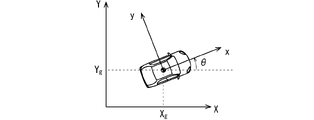
- FIG. 3 is a diagram showing an example of a coordinate system according to the first embodiment.
- X and Y in FIG. 3 represent the inertial coordinate system
- X g , Y g , and ⁇ represent the center-of-gravity position and vehicle body orientation of the own vehicle in the inertial coordinate system.
- x and y are an own vehicle coordinate system in which the center of gravity of the own vehicle is the origin, the x axis is in front of the own vehicle, and the y axis is in the left hand direction.
- the center-of-gravity positions X g and Y g of the own vehicle and the vehicle body orientation ⁇ are initialized to 0 in each of the first execution period and the second execution period. In other words, the inertial coordinate system and the own vehicle coordinate system are made to match each of the first execution period and the second execution period.
- the first trajectory generation unit 240 and the second trajectory generation unit 260 are optimized to find the control input u that minimizes the evaluation function J representing the desired behavior of the own vehicle under the constraint g. solve the transformation problem.
- the first trajectory generator 240 and the second trajectory generator 260 generate current time 0 based on the control input u obtained from the optimization problem and the vehicle model f that mathematically expresses the motion of the own vehicle. to the future of the prediction period T h at the prediction interval T s .
- the time from the current time to Th may be abbreviated as horizon.
- the first trajectory generator 240 and the second trajectory generator 260 generate a trajectory ⁇ , which is series data including the position of the own vehicle, from the optimized vehicle state quantity.
- the generation of this trajectory ⁇ is executed at a constant execution cycle Te.
- the vehicle model f, constraint g, evaluation function J, prediction interval T s , prediction period T h , and execution period T e differ between the first trajectory generation unit 240 and the second trajectory generation unit 260.
- trajectory generator 240 when explicitly distinguishing these variables between the first trajectory generator 240 and the second trajectory generator 260, for example, the first vehicle model f1 and the second prediction interval T It is written as s,2 . Further, series data including the position of the own vehicle is denoted as trajectory ⁇ , and series data including only the position of the own vehicle is denoted as route ⁇ .
- the order of the second vehicle model f2 is greater than the order of the first vehicle model f1. According to such a configuration, since the trajectory is generated by the detailed second vehicle model f2 based on the trajectory generated by the simple first vehicle model f1, the detailed second vehicle model f 2 can be reduced.
- the second prediction period T h,2 is shorter than the first prediction period T h,1 . Therefore, a long-term trajectory can be generated with the simple first vehicle model f1, and a short-term trajectory can be generated with the detailed second vehicle model f2.
- the first trajectory is smooth because it is a long-term trajectory, but it is generated from a simple first vehicle model, so it is not suitable for use in calculating target values.
- the second trajectory is generated from a refined vehicle model, it is suitable for use in calculating target values.
- the second trajectory is a short-term trajectory, it is generated based on the first trajectory, so the smoothness of the second trajectory is ensured.
- the first embodiment it is possible to generate a smooth trajectory that allows the own vehicle to run smoothly while suppressing an increase in the computational load, and precisely control the own vehicle. can be compatible.
- the first prediction period T h,1 is the product of the prediction score N 1 and the first prediction interval T s,1
- the second prediction period T h,2 is the prediction score N 2 and the second prediction interval T s,1
- the prediction scores N 1 and N 2 may be the same and constant when they are the product of the prediction interval T s,2 . As a result, even if the prediction period becomes longer, it is possible to suppress an increase in computational load.
- the computation load depends on the order of the vehicle model and the number of prediction points N (prediction period Th divided by prediction interval Ts ).
- the second prediction period T h,2 2.0 [sec]
- the second prediction interval T s,2 0.1 [sec]
- the second prediction score N2 can be reduced to 30 [points] as described above. As a result, it is possible to minimize the increase in computational load due to the generation of the second trajectory.
- the first prediction interval T s,1 and the second prediction interval T s,2 are the same 0.1 [sec]. It may be smaller than one prediction interval T s,1 . As a result, the time resolution when generating the second trajectory is increased, and more precise vehicle control can be achieved. However, it is desirable to set the second prediction interval T s,2 so that the second prediction score N2 is not larger than the first prediction score N1 as much as possible.
- the second execution period T e,2 for generating the second trajectory may be set to be less than or equal to the first execution period T e,1 for generating the first trajectory.
- the second trajectory generator 260 which directly affects the target value of the own vehicle, is executed at a high frequency while securing the calculation time in the first trajectory generator 240 for generating a long-term trajectory. Therefore, it is possible to achieve both generation of a smooth trajectory and precise control of the own vehicle.
- the parameters in the first trajectory generation and the parameters in the second trajectory generation are: first prediction period T h,1 > second prediction period T h,2 , first prediction interval T s, It is desirable to set such that 1 ⁇ second prediction interval T s,2 , and first execution cycle T e,1 ⁇ second execution cycle T e,2 .
- the first trajectory generator 240 and the second trajectory generator 260 solve the constrained optimization problem at regular intervals.
- the optimization problem is formulated as follows.
- J is an evaluation function
- x is a vehicle state quantity
- u is a control input
- f is a vector-valued function related to a dynamic vehicle model
- x0 is an initial value of a vehicle state quantity, ie, a current vehicle state quantity
- g is a vector-valued function relating to constraints, and is a function for setting upper and lower limits of vehicle state quantity x and control input u in a constrained optimization problem. Optimization that minimizes the evaluation function J is performed under the constraint g(x,u) ⁇ 0.
- h is the vector-valued function for the evaluation item
- hN is the vector-valued function for the evaluation item at the end (prediction score N )
- W and WN are weight matrices, which are diagonal matrices having weights for each evaluation item in their diagonal components, and can be changed as parameters of the evaluation function J as appropriate.
- the first vehicle state quantity x1 and the first control input u1 used in the first trajectory generator 240 are set as follows.
- X g and Y g are the positions of the center of gravity of the own vehicle in FIG. 3
- V is the vehicle speed
- ⁇ is the steering angle
- a is the acceleration
- ⁇ is the steering angular velocity.
- the first vehicle state quantity x1 and the first control input u1 may be set arbitrarily as long as the first vehicle state quantity x1 includes a variable related to the position.
- the positional variable is not limited to the orthogonal coordinate system, and may be defined by, for example, the path coordinate system, and the positional variable may not be the barycentric position.
- ⁇ is the sideslip angle and ⁇ is the yaw rate, which are expressed by the following equation in the first trajectory generator 240.
- a vehicle model other than a geometric model may be used as the first vehicle model f1.
- the second vehicle state quantity x2 and the second control input u2 used in the second trajectory generator 260 are set as follows.
- the second vehicle state quantity x2 includes a variable related to position, and either the second vehicle state quantity x2 or the second control input u2 includes a variable related to steering and vehicle speed. Then, the second vehicle state quantity x2 and the second control input u2 may be set in any way. Further, the positional variable is not limited to the orthogonal coordinate system, and may be defined by, for example, the path coordinate system, and the positional variable may not be the barycentric position.
- the second vehicle state quantity x2 includes a variable related to position, and the variable related to steering includes the second vehicle state quantity x2 and the second control input u2.
- the second vehicle state quantity x2 and the second control input u2 may be set in any way.
- T a and T ⁇ are time constants when the followability to acceleration and steering angle commands is represented by a first-order lag system.
- Y f and Y r are the cornering forces of the front and rear wheels, which are expressed by the following equations using the cornering stiffnesses C f and Cr of the front and rear wheels.
- a vehicle model other than the two-wheel model may be used as the second vehicle model f2.
- the second vehicle model f2 For example, on a straight road without obstacles, it is not always necessary to use a precise two-wheel model. It may be used for model f2 .
- the second trajectory generator 260 selects a vehicle model according to road conditions, it may be possible to further suppress an increase in computational load.
- the state of the road is, for example, the curvature of the road acquired by the road information acquisition unit 120 .
- the second trajectory generator 260 may change the order of the vehicle model according to road conditions.
- FIG. 4 is a flow chart showing an example of the procedure of automatic driving of own vehicle according to the first embodiment.
- the obstacle information acquisition unit 110 acquires obstacle information.
- the obstacle information is information including the position of the obstacle.
- the right front edge of the obstacle in the own vehicle coordinate system when the obstacle exists to the left front of the own vehicle, the right front edge of the obstacle in the own vehicle coordinate system. Including the positions of P FR , right rear edge P RR and left rear edge P RL , and when an obstacle exists in the right front of the own vehicle, left front edge P FL of the obstacle in the own vehicle coordinate system, The positions of the left rear end P RL and the right rear end P RR shall be included.
- the obstacle information acquisition unit 110 determines the position of the left front end PFL or the right front end PFR of the obstacle, the positions Xo and Yo of the center PC, the vehicle body direction ⁇ o , and the speed Vo . , length l o and width w o .
- the road information acquisition unit 120 acquires road information.
- the road information is information including the boundary of the road on which the vehicle is traveling, and in the first embodiment, is information including coefficients when the left and right lane markings are expressed by a third-order polynomial. That is, the road information acquisition unit 120 acquires the values of c l0 to c l3 of formula 201 for the left lane marking, and the values of c r0 to c r3 of formula 202 for the right lane marking. get.
- the center of the lane is expressed by the following formula.
- section line information is not limited to the cubic polynomial as described above, and may be expressed by any function.
- the vehicle information acquisition unit 130 acquires vehicle information, which is the current vehicle state quantity of the own vehicle.
- vehicle information is information of the vehicle state quantity x such as the steering angle, yaw rate, speed, acceleration, etc. of the own vehicle or information for estimating the vehicle state quantity x. ⁇ , velocity V, and acceleration a.
- the vehicle state quantity estimation unit 210 estimates the current vehicle state quantity x of the own vehicle based on the vehicle information acquired by the vehicle information acquisition unit .
- Known techniques such as a low-pass filter, observer, Kalman filter, and particle filter are used for estimating the vehicle state quantity x.
- the obstacle movement prediction unit 220 predicts the movement of the obstacle based on the obstacle information acquired by the obstacle information acquisition unit 110.
- X o,0 , Y o,0 , ⁇ o,0 , V o,0 are the center position, vehicle direction, and speed of the obstacle at the current time acquired by the obstacle information acquisition unit 110 . If there are multiple obstacles, the above prediction is made for each obstacle. Note that the obstacle movement prediction unit 220 may predict the movement of the obstacle assuming that the obstacle moves along the driving lane at a constant speed, instead of as a uniform linear motion. Alternatively, the obstacle movement prediction unit 220 may use the driver model to predict the movement of the obstacle.
- the first place setting unit 230 based on the obstacle information acquired by the obstacle information acquiring unit 110 and the road information acquired by the road information acquiring unit 120, sets the first Set up the field S1 .
- a field of 1 is set as S1.
- l a and l b are the lengths of the major axis and minor axis of the ellipse set for the obstacle, respectively, and may be changed for each prediction point k. Also, the center of the ellipse need not coincide with the center positions X o,k and Y o,k of the obstacles. Also, the prohibited entry area set for the obstacle does not have to be elliptical, and any shape of prohibited entry area may be set. When there are a plurality of obstacles, the first field setting unit 230 sets a no-entry area for each obstacle.
- step S240 of FIG. 4 the first trajectory generator 240 generates the first vehicle model f1, the first field S1, the first evaluation function J1, and the first constraint g1.
- the first trajectory ⁇ 1 is generated based on the road information and the first vehicle state quantity x 1 . Note that the processing of step S240 will be described later in detail.
- the second place setting unit 250 selects the second location based on the obstacle information acquired by the obstacle information acquisition unit 110 and the road information acquired by the road information acquisition unit 120.
- Set up the field S2 For example, similarly to the first field setting unit 230, the second field setting unit 250 calculates the obstacle center positions X o,k , Y o, An elliptical keep-out area obtained by applying Equation 209 to k is set as the second field S2.
- the lengths l a and l b of the major axis and minor axis of the ellipse in the second field S 2 may be values different from those set in the first field S 1 .
- the no-entry area set for the obstacle does not have to be elliptical, and any shape of no-entry area may be set.
- the second field setting unit 250 sets a no-entry area for each obstacle.
- step S260 of FIG. 4 the second trajectory generator 260 generates a second vehicle model f2, a second field S2, a second evaluation function J2, and a second constraint g2. , generates a second trajectory ⁇ 2 based on the first trajectory ⁇ 1 and the second vehicle state quantity x 2 .
- the processing of step S260 will be described later in detail.
- the target value calculator 270 calculates the target value based on the second trajectory ⁇ 2.
- the target value calculation unit 270 calculates the target steering angle ⁇ t , which is a target value for steering, and A target acceleration at, which is a target value, is calculated.
- the value calculation unit 270 calculates the target steering angle ⁇ t and the target acceleration at by interpolating the target steering angle ⁇ t ,k and the target acceleration at ,k with respect to time according to the control cycle of each actuator. .
- the target value calculation section 270 calculates the target steering angle ⁇ t and Precise vehicle control is realized by calculating the target acceleration at.
- actuator control section 310 controls the actuator based on the target value calculated by target value calculation section 270 .
- the EPS motor 5 is controlled so that the steering angle ⁇ follows the target steering angle ⁇ t
- the power train unit 6 and the brake unit 7 are controlled so that the acceleration a follows the target acceleration at. be done.
- FIG. 5 is a flowchart showing an example of the first trajectory generation procedure according to the first embodiment. This process is performed in step S240 of FIG.
- the first trajectory generator 240 sets the first constraint g 1 (x 1 , u 1 ) ⁇ 0.
- the subscript of N1 is represented as N1 due to notational restrictions.
- the first constraint g1 includes a constraint that prohibits the vehicle from entering the first field S1.
- ⁇ a, _a, ⁇ , _ ⁇ are the upper and lower limits of each control input. Due to notational restrictions in the text of this specification, the symbol “_” represents an underscore attached to the following character, and the symbol “ ⁇ ” represents an overscore attached to the following character.
- the upper limit value and lower limit value of each control input may be changed for each prediction point k. In the first embodiment, restrictions are set only on the center-of-gravity positions X g and Y g and the first control input u 1 . may
- the first trajectory generator 240 sets the first evaluation function J1 as shown in Equation 103.
- the first trajectory generator 240 can generate a first trajectory for the host vehicle to travel along the reference route at the reference vehicle speed, and
- the first vector-valued functions h 1 , h 1 , N1 relating to the evaluation items are set as shown in the following equations so that the control input at that time is small.
- the reference values r 1,k , r 1,N1 in Equation 103 are set as follows.
- the first trajectory generator 240 when no obstacle exists within the horizon, the first trajectory generator 240 generates a first trajectory for the host vehicle to follow the first reference route at the reference vehicle speed with a small control input. can.
- heading, yaw rate, lateral acceleration, and the like may be added to the evaluation items of the first evaluation function J1.
- the first trajectory generation unit 240 for example, in the case of control in which the host vehicle runs in the center of the lane, based on the X position, Y position, and direction of the center of the lane indicated by the road information, the reference position X r,k , Y r,k and the reference vehicle heading ⁇ r,k are determined.
- a condition is set between the reference position X r,k , Y r,k and the reference vehicle speed V r,k for their matching. That is, the first trajectory generator 240 determines the reference positions X r,k and Y r,k so as to satisfy the following two expressions.
- Equation 309 indicates that the interval between the adjacent reference positions X r,k ⁇ 1 , Y r,k ⁇ 1 and X r,k , Y r,k is the movement of the own vehicle at the first prediction interval T s,1 . It is a condition for equality in quantity.
- the first trajectory generation unit 240 generates the first evaluation function J1 of Equation 103 reflecting the road information and the first vehicle state quantity x1, and the first field S1
- the first optimal control input u 1 * is obtained by solving the constrained optimization problem based on the first constraint g 1 of Equations 301 and 302 in which is reflected.
- the calculation for obtaining the first optimum control input u 1 * is performed using K.K. U.S.A.
- Known means such as ACADO (Automatic Control And Dynamic Optimization) developed by the University of Leuven and AutoGen, which is an automatic code generation tool for solving optimization problems based on the C/GMRES method, are used.
- a 1,k * and ⁇ 1,k * of each prediction point k are the first optimum acceleration and the first optimum steering angular velocity.
- the solution may be a value such that the first evaluation function J1 falls below a predetermined threshold.
- the solution may be the value that minimizes the function J1.
- the first trajectory generator 240 outputs the first optimum state quantity x 1 * of the following equation in step S244.
- the series data of the position in the first optimum state quantity x 1 * is referred to as the first optimum path ⁇ 1 * .
- the first optimal path ⁇ 1 * is represented by the following equation.
- the first trajectory generator 240 generates the first trajectory ⁇ 1 based on the first optimum state quantity x1 * and the first optimum control input u1 * .
- the first trajectory ⁇ 1 may include the first optimum center-of-gravity position X g,1 * , Y g,1 * , the optimum vehicle orientation ⁇ 1 * , and the optimum vehicle speed V 1 *.
- the first optimum state quantity x 1 * is the first trajectory ⁇ 1 . That is, in step S245, the first trajectory generator 240 outputs the first trajectory ⁇ 1 of the following equation.
- the series data of the position in the first trajectory ⁇ 1 is referred to as the first path ⁇ 1.
- the first path ⁇ 1 is expressed by the following equation.
- FIG. 6 is a flow chart showing an example of the second trajectory generation procedure according to the first embodiment. This process is performed in step S260 of FIG.
- the second trajectory generator 260 sets a second constraint g 2 (x 2 , u 2 ) ⁇ 0.
- the second constraint g2 includes a constraint that prohibits the vehicle from entering the second field S2.
- ⁇ jr, _jr , ⁇ ⁇ r , _ ⁇ r are the upper and lower limits of each control input .
- the upper limit value and lower limit value of each control input may be changed for each prediction point k.
- only the center-of-gravity positions X g and Y g and the second control input u 2 are restricted, but the yaw rate, lateral acceleration, etc. are restricted in order to improve the ride comfort.
- the second trajectory generator 260 sets the second evaluation function J2 as shown in Equation 103.
- the second trajectory generator 260 can generate a second trajectory for the host vehicle to follow the first trajectory at the speed of the first trajectory, and the control input at that time
- a second vector-valued function h 2 , h 2 , N2 related to the evaluation item is set as follows so that .
- e Y and k are represented by the following equations.
- the reference values r 2,k , r 2,N2 in Equation 103 are set as follows.
- the second trajectory generator 260 uses part of the first trajectory ⁇ 1 as the second reference path ⁇ r,2 to generate the second trajectory.
- the second trajectory generation unit 260 sets the reference positions X r,k , Y r,k , the reference The vehicle body direction ⁇ r,k and the reference vehicle speed V r,k are determined on a case-by-case basis.
- the second trajectory generation unit 260 when the first prediction interval T s,1 and the second prediction interval T s,2 are equal, the second trajectory generation unit 260 generates reference positions X r,k , Y r,k , reference The vehicle azimuth ⁇ r,k and the reference vehicle speed V r,k are determined by the following equations.
- the second trajectory generation unit 260 calculates the first optimum center-of-gravity position X g,1 * , Time is appropriately interpolated so that the interval between Y g,1 * , the optimum vehicle heading ⁇ 1 * , and the optimum vehicle speed V 1 * coincides with the second prediction interval T s,2 , and the reference position X r,k , Y r,k , reference vehicle heading ⁇ r,k , and reference vehicle speed V r,k are determined.
- the second trajectory generator 260 can generate a second trajectory for the host vehicle to follow the first route at the speed of the first trajectory with a small control input.
- the azimuth, yaw rate, lateral acceleration, etc. may be added to the evaluation items of the second evaluation function J2.
- the second trajectory generation unit 260 generates the second evaluation function J2 of Equation 103 reflecting the first trajectory and the second vehicle state quantity x2, and the second field
- the second optimal control input u 2 * is determined by solving the constrained optimization problem based on the second constraint g 2 of equation 401 and equation 402 reflecting S 2 .
- a method similar to the calculation for the first optimum control input can be used for the calculation for obtaining the second optimum control input u 2 * .
- the second trajectory generator 260 may determine an initial solution based on the first trajectory ⁇ 1 when solving the optimization problem. Since the second trajectory ⁇ 2 and the first trajectory ⁇ 1 are similar unless the obstacle moves significantly beyond the movement prediction, determining the initial solution based on the first trajectory ⁇ 1 yields the first 2, the speed of computing the optimal control input u 2 * is improved.
- the second trajectory generator 260 outputs the second optimum state quantity x 2 * of the following equation in step S264.
- the second optimal path ⁇ 2 * is represented by the following equation.
- the second trajectory generator 260 generates the second trajectory ⁇ 2 based on the second optimum state quantity x2 * and the second optimum control input u2 * .
- the second trajectory ⁇ 2 may include the second optimum steering angle ⁇ 2 * and the second optimum acceleration a 2 * .
- the series data of the position in the second trajectory ⁇ 2 is referred to as the second path ⁇ 2.
- the second path ⁇ 2 is expressed by the following equation.
- the order of the second vehicle model f2 is higher than the order of the first vehicle model f1. According to such a configuration, since the trajectory is generated by the detailed second vehicle model f2 based on the trajectory generated by the simple first vehicle model f1, the detailed second vehicle model f 2 can be reduced.
- the long-term trajectory is generated by the simple first vehicle model f1, and the refined second vehicle model f1 is generated.
- a short - term trajectory can be generated with the vehicle model f2. Therefore, it is possible to achieve both the generation of a smooth trajectory that allows the vehicle to run smoothly and the precise control of the vehicle, while suppressing an increase in computational load.
- a block diagram of the control arithmetic device 201 according to the second embodiment is the same as the block diagram of FIG.
- the constituent elements that are the same as or similar to the constituent elements of the first embodiment are denoted by the same or similar reference numerals, and different constituent elements will be mainly described. Note that this also applies to the second and subsequent embodiments.
- the second field may be the same as or different from the first field, but in Embodiment 2, the second field is different from the first field. different.
- FIG. 7 is a schematic diagram showing an example of the relationship between the first field S1 and the first path ⁇ 1 according to the second embodiment.
- the preceding vehicle which is an obstacle on the left front, is stopped or traveling parallel to the lane.
- the own vehicle runs in the center of the lane as much as possible while avoiding obstacles.
- the fact that the lane is a straight road is an example, and the road may not be a straight road.
- the number of lanes is three in the example of FIG. 7, it is not limited to this.
- the first field setting section 230 uses the method described in step S230 to form an elliptical shape.
- a first field S1 is set up containing a no entry area of .
- the major axis a and the minor axis b of the ellipse are set, for example, so as to include a collision area SC, which is an area where the vehicle collides with an obstacle when the center of gravity of the vehicle enters.
- the first trajectory generator 240 does not enter the first field S1 and does not enter the first field S1 from the center of the lane as much as possible.
- a path that does not leave is generated as the first path ⁇ 1.
- FIG. 8 is a schematic diagram showing an example of the relationship between the first path ⁇ 1, the second field S2, and the second path ⁇ 2 according to the second embodiment.
- the second field setting unit 250 sets the second field S2 including the elliptical no-entry area by the method described in step S250 based on the surrounding information.
- the second field setting unit 250 includes the collision area Sc and the major axis a and the minor axis b is less than the first field S1.
- the second trajectory generator 260 sets the first route ⁇ 1 as the second reference route ⁇ r ,2 .
- the second field S2 is smaller than the first field S1, an obstacle
- the first path ⁇ 1 which is the second reference path ⁇ r,2 , does not overlap with the second field S 2 as long as S 1 does not move significantly beyond the movement prediction.
- the second optimal control input obtained as the solution of the optimization problem in the second trajectory generation unit 260 in step S263 is less likely to conflict with the constraints imposed by the second field S2. 2, the calculation speed in the second optimum control input of the trajectory generator 260 is improved.
- the second route ⁇ 2 may be almost the same as the first route ⁇ 1, the second trajectory generation using the detailed second vehicle model f2 An increase in the calculation load of the unit 260 can be reduced.
- the second route ⁇ 2 obtained in step S265 follows the first route ⁇ 1 while reflecting the vehicle motion of the second vehicle model f2. .
- FIG. 9 is a schematic diagram showing another example of the relationship between the first path ⁇ 1, the second field S2, and the second path ⁇ 2 according to the second embodiment.
- the obstacle has moved significantly beyond the movement prediction from the completion of the processing of the first trajectory generation unit 240 shown in FIG. 7 to the start of the processing of the second trajectory generation unit 260. It is shown.
- first execution period T e,1 when the first execution period T e,1 is longer than the second execution period T e,2 and the first execution period T e,1 is long, such as one second, Alternatively, for example, it may occur when the accuracy of the sensor of the obstacle information acquisition unit 110 is low.
- the obstacle has moved far beyond the predicted movement, so when the own vehicle follows the first route ⁇ 1, it collides with the obstacle.
- a route that does not enter the second field S2 can be obtained as the second route ⁇ 2. Vehicles can avoid collisions with obstacles and ensure safety.
- the portion where the second field S2 and the first path ⁇ 1 of the first trajectory ⁇ 1 overlap is where the first field S1 and the first path ⁇ 1 of the first trajectory ⁇ 1 are Since it is smaller than the overlapping portion, it is possible to reduce an increase in the calculation load of the second trajectory generator 260 that uses the detailed second vehicle model f2.
- the first route ⁇ 1 is considered when calculating the second route ⁇ 2, the divergence between the second route ⁇ 2 and the first route ⁇ 1 is reduced as much as possible. , and the increase in computational load on the second trajectory generator 260 can be reduced.
- the portion where the second field S2 and the first path ⁇ 1 of the first trajectory ⁇ 1 overlap is where the first field S1 and the first path ⁇ 1 of the first trajectory ⁇ 1 Less than overlap may include that the second field S 2 does not overlap with the first path ⁇ 1 or does overlap. Also, if the overlapping portion of the second field S2 and the first path ⁇ 1 is smaller than the overlapping portion of the first field S1 and the first path ⁇ 1, then the second field S2 need not be less than the first field S1.
- the second field S2 may be a field obtained by moving the first field S1 in the traveling direction of the vehicle while maintaining the area on the XY plane.
- Embodiment 3 the second field S2 and the first path ⁇ 1 are overlapped so that the overlapped area between the first field S1 and the first path ⁇ 1 is smaller than the overlapped area between the first field S1 and the first path ⁇ 1.
- the second scene setting unit 250 sets the second scene S2.
- the portion where the second field S2 and the first path ⁇ 1 overlap is larger than the portion where the first field S1 and the first path ⁇ 1 overlap.
- the second field setting unit 250 sets the second field S2 such that
- the linearization error can be reduced by using a reference route with a small difference from the optimum route as the initial solution.
- FIG. 10 is a schematic diagram showing an example of the relationship between the first field S1 and the first path ⁇ 1 according to the third embodiment.
- FIG. 11 is a schematic diagram showing an example of the relationship between the first path ⁇ 1, the second field S2, and the second path ⁇ 2 according to the third embodiment.
- the first field setting unit 230 sets a first field S1 having a minimum size that can contain the collision area SC .
- the difference of the first route ⁇ 1 from the lane center, which is the reference route becomes small. This makes it possible to reduce the calculation load in the first trajectory generation unit 240, reduce the possibility of falling into a local optimum solution, and reduce the linearization error.
- the distance between the vehicle and the obstacle when avoiding the obstacle that is, the avoidance distance
- the second field setting unit 250 sets a second field S2 larger than the first field S1.
- the first route ⁇ 1 has a small margin in the avoidance interval
- the second route ⁇ 2 has a margin in the avoidance interval, improving safety.
- the second trajectory generator 260 sets the first route ⁇ 1 as the second reference route ⁇ r ,2 , the difference between the reference route and the optimum route is greater than when the center of the lane is used as the reference route. the difference between Therefore, it is possible to reduce the calculation load in the second trajectory generation, reduce the possibility of falling into a local optimum solution, and reduce the linearization error.
- the first field S1 is a no-entry area for obstacles, but it is not limited to this.
- the first field S1 may be a potential field of risk according to the degree of proximity corresponding to the distance between the center of the first field and the host vehicle.
- the center of the first field referred to here may be a center point, an obstacle, or a no-entry area.
- the variable of the first evaluation function J1 is the degree of proximity corresponding to the distance between the center of the first field S1 and the own vehicle, such as the repulsive force according to the distance. contains parameters related to the potential field of As a result, in the constraints used in the first trajectory generation unit 240, the constraints relating to the obstacle avoidance position are relaxed, thereby improving the possibility of finding the optimum solution. However, since the first trajectory generation unit 240 cannot clearly specify the avoidance interval between the vehicle and the obstacle when avoiding the obstacle, the vehicle may not be able to avoid the obstacle only by using the first trajectory generator 240 . Therefore, in the fourth embodiment, the no-entry area is used for the second field S2. As a result, the avoidance interval can be clearly designated by the second trajectory generator 260, so that the own vehicle can reliably avoid the obstacle.
- FIG. 12 is a schematic diagram showing an example of the relationship between the first field S1 and the first path ⁇ 1 according to the fourth embodiment.
- FIG. 13 is a schematic diagram showing an example of the relationship between the first path ⁇ 1, the second field S2, and the second path ⁇ 2 according to the fourth embodiment.
- the first field S1 is a potential field of risk according to the degree of proximity to an obstacle.
- the constraint on the obstacle avoidance position is relaxed in the first trajectory generation, and the possibility of finding the optimum solution is improved.
- the avoidance interval cannot be specified clearly in the first trajectory generator 240, there is a possibility that the own vehicle cannot completely avoid the obstacle depending on the design of the first evaluation function J1.
- the second field setting unit 250 sets the second field S2 so as to include the collision area SC.
- the avoidance interval can be clearly designated by the second trajectory generator 260, so that the own vehicle can reliably avoid the obstacle.
- the second trajectory generator 260 sets the first route ⁇ 1 as the second reference route ⁇ r ,2 , the difference between the reference route and the optimum route is greater than when the center of the lane is used as the reference route. the difference between Therefore, it is possible to reduce the calculation load in the second trajectory generation, reduce the possibility of falling into a local optimum solution, and reduce the linearization error.
- the variables of the second evaluation function J2 are , the proximity corresponding to the distance between the center of the second field S2 and the host vehicle.
- the first field S1 and the second field S2 are set for obstacles, but they may be set for road boundaries.
- the second field S2 of the boundary of the road is set in the same way as the second field S2 of the obstacle.
- the first field S1 is larger than at least one area of the obstacle and the road
- the second field S2 is larger than the at least one area
- the first path ⁇ 1 which is the reference path of the second trajectory generator 260, does not overlap the second field S2, and the solution of the optimization problem by the second trajectory generator 260 is the second Since the possibility of infringing on the constraint by the field S2 is reduced, the calculation load of the second trajectory generation unit 260 can be reduced.
- FIG. 14 is a schematic diagram showing an example of the relationship between the first field S1 and the first path ⁇ 1 according to the fifth embodiment.
- FIG. 15 is a schematic diagram showing an example of the relationship between the first path ⁇ 1, the second field S2, and the second path ⁇ 2 according to the fifth embodiment.
- the first field S1 is set as an entry prohibited area with respect to the border of the road. However, the first field S1 is set slightly larger than the boundary of the road.
- the second field S2 is set as a no-entry area with respect to the border of the road.
- the second field S2 is a road area and is set to be smaller than the first field S1.
- the first path ⁇ 1 which is the reference path of the second trajectory generator 260, does not overlap the second field S2, and the solution of the optimization problem by the second trajectory generator 260 is the second Since the possibility of infringing on the constraint by the field S2 is reduced, the calculation load of the second trajectory generation unit 260 can be reduced.
- Embodiments 2 and 5 mention that the solution of the optimization problem by the second trajectory generator 260 is less likely to conflict with the constraint by the second field S2. This is achieved by appropriately setting the second field S2.
- a method of setting the first constraint g 1 when generating the first trajectory and the second constraint g 2 when generating the second trajectory will be described.
- constraints may be set not only on the position of the host vehicle and control inputs, but also on speed, lateral acceleration, steering angle, yaw rate, and the like. Then, the second constraint g2 is set looser than the first constraint g1. For example, in the first constraint g 1 , upper and lower limit values ⁇ 1 and _ ⁇ 1 are set for the steering angle ⁇ . Similarly, in the second constraint g 2 , upper and lower limit values ⁇ 2 and _ ⁇ 2 are set for the steering angle ⁇ .
- the first trajectory generated by the first trajectory generation unit 240 satisfies the second constraint g2. less likely to conflict.
- the second trajectory generation unit 260 generates the second trajectory, the possibility that the second trajectory will conflict with the second constraint g2 is reduced. can reduce the computational load of
- the first field setting unit 230, the first trajectory generation unit 240, the second field setting unit 250, the second trajectory generation unit 260, and the target value calculation unit 270 in FIG. field setting unit 230, etc.” are realized by the processing circuit 81 shown in FIG. That is, the processing circuit 81 includes a first field setting unit 230 that sets a first field outside the target of vehicle travel, a first vehicle model representing the motion of the vehicle, and a first field based on the surrounding information.
- a first trajectory generation unit 240 that generates a first trajectory of the vehicle in the first prediction period based on the field and a second trajectory that is different from the first field and is not subject to travel of the vehicle based on the surrounding information.
- a second field setting unit 250 for setting a field of, a second vehicle model representing vehicle motion and having a higher order than the first vehicle model, a second field, and a first trajectory based on a second trajectory generator 260 for generating a second trajectory of the vehicle for a second prediction period that is equal to or shorter than the first prediction period; and a target value for controlling the vehicle based on the second trajectory. and a target value calculation unit 270 for calculating and outputting.
- Dedicated hardware may be applied to the processing circuit 81, or a processor that executes a program stored in a memory may be applied.
- Processors include, for example, central processing units, processing units, arithmetic units, microprocessors, microcomputers, and DSPs (Digital Signal Processors).
- the processing circuit 81 may be, for example, a single circuit, a composite circuit, a programmed processor, a parallel programmed processor, an ASIC (Application Specific Integrated Circuit), an FPGA (Field Programmable Gate Array), or a combination of these.
- Each function of each unit such as the first field setting unit 230 may be realized by a circuit in which processing circuits are distributed, or the functions of each unit may be collectively realized by one processing circuit.
- the processing circuit 81 When the processing circuit 81 is a processor, the functions of the first field setting unit 230 and the like are realized by combining with software and the like.
- Software and the like correspond to, for example, software, firmware, or software and firmware.
- Software or the like is written as a program and stored in memory. As shown in FIG. 17, a processor 82 applied to a processing circuit 81 reads out and executes a program stored in a memory 83 to implement the functions of each section.
- control arithmetic unit 201 when executed by the processing circuit 81, based on the surrounding information, the step of setting a first field outside the object of vehicle travel; and a step of generating a first trajectory of the vehicle in a first prediction period based on the first field; a first prediction period based on the step of establishing a field, a second vehicle model representing vehicle motion and having a greater order than the first vehicle model, the second field, and the first trajectory; Generating a second trajectory of the vehicle for a second prediction period that is
- a memory 83 is provided for storing programs to be executed. In other words, it can be said that this program causes a computer to execute the procedures and methods of the first place setting unit 230 and the like.
- the memory 83 is, for example, RAM, ROM, flash memory, EPROM (Erasable Programmable Read Only Memory), EEPROM (Electrically Erasable Programmable Read Only Memory), non-volatile or volatile semiconductor memory, HDD (Hard Disk Drive), a magnetic disk, a flexible disk, an optical disk, a compact disk, a mini disk, a DVD (Digital Versatile Disc), a drive device thereof, or any storage medium that will be used in the future.
- each function of the first place setting unit 230 and the like is realized by either hardware or software has been described above.
- the configuration is not limited to this, and a configuration in which a part of the first field setting unit 230 and the like is realized by dedicated hardware and another part is realized by software or the like may be employed.
- the function of the first field setting unit 230 is realized by a processing circuit 81, an interface, a receiver, etc. as dedicated hardware, and the processing circuit 81 as a processor 82 is stored in the memory 83 for the rest.
- the function can be realized by reading and executing the program.
- the processing circuit 81 can implement each of the functions described above by means of hardware, software, etc., or a combination thereof.
- control arithmetic device described above includes vehicle devices such as PND (Portable Navigation Device), navigation device and DMS (Driver Monitoring System), communication terminals including mobile terminals such as mobile phones, smartphones and tablets, and vehicles
- vehicle devices such as PND (Portable Navigation Device), navigation device and DMS (Driver Monitoring System), communication terminals including mobile terminals such as mobile phones, smartphones and tablets, and vehicles
- the present invention can also be applied to a control operation system constructed as a system by appropriately combining functions of an application installed in at least one of a device and a communication terminal and a server.
- each function or each component of the control arithmetic unit described above may be distributed to each device that constructs the system, or may be centrally disposed in any one of the devices. .
- 1 own vehicle 201 control arithmetic device, 230 first field setting unit, 240 first trajectory generation unit, 250 second field setting unit, 260 second trajectory generation unit, 270 target value calculation unit.
Landscapes
- Engineering & Computer Science (AREA)
- Automation & Control Theory (AREA)
- Transportation (AREA)
- Mechanical Engineering (AREA)
- Human Computer Interaction (AREA)
- Steering Control In Accordance With Driving Conditions (AREA)
- Control Of Driving Devices And Active Controlling Of Vehicle (AREA)
Priority Applications (4)
| Application Number | Priority Date | Filing Date | Title |
|---|---|---|---|
| US18/276,505 US20240116506A1 (en) | 2021-04-28 | 2021-04-28 | Control calculation apparatus and control calculation method |
| PCT/JP2021/016923 WO2022230094A1 (ja) | 2021-04-28 | 2021-04-28 | 制御演算装置及び制御演算方法 |
| DE112021007599.3T DE112021007599T5 (de) | 2021-04-28 | 2021-04-28 | Steuerberechnungsvorrichtung und Steuerberechnungsverfahren |
| JP2023516939A JP7337302B2 (ja) | 2021-04-28 | 2021-04-28 | 制御演算装置及び制御演算方法 |
Applications Claiming Priority (1)
| Application Number | Priority Date | Filing Date | Title |
|---|---|---|---|
| PCT/JP2021/016923 WO2022230094A1 (ja) | 2021-04-28 | 2021-04-28 | 制御演算装置及び制御演算方法 |
Publications (1)
| Publication Number | Publication Date |
|---|---|
| WO2022230094A1 true WO2022230094A1 (ja) | 2022-11-03 |
Family
ID=83848008
Family Applications (1)
| Application Number | Title | Priority Date | Filing Date |
|---|---|---|---|
| PCT/JP2021/016923 Ceased WO2022230094A1 (ja) | 2021-04-28 | 2021-04-28 | 制御演算装置及び制御演算方法 |
Country Status (4)
| Country | Link |
|---|---|
| US (1) | US20240116506A1 (https=) |
| JP (1) | JP7337302B2 (https=) |
| DE (1) | DE112021007599T5 (https=) |
| WO (1) | WO2022230094A1 (https=) |
Families Citing this family (3)
| Publication number | Priority date | Publication date | Assignee | Title |
|---|---|---|---|---|
| GB2621317B (en) * | 2022-07-26 | 2024-09-11 | Jaguar Land Rover Ltd | Determination of autonomous manoeuvring control configurations |
| US12337878B2 (en) | 2022-11-30 | 2025-06-24 | Zoox, Inc. | Prediction model with variable time steps |
| US12428032B2 (en) * | 2022-11-30 | 2025-09-30 | Zoox, Inc. | Determining prediction times for a model |
Citations (3)
| Publication number | Priority date | Publication date | Assignee | Title |
|---|---|---|---|---|
| JP2007253745A (ja) * | 2006-03-22 | 2007-10-04 | Nissan Motor Co Ltd | 回避操作算出装置、回避制御装置、各装置を備える車両、回避操作算出方法および回避制御方法 |
| JP2020163967A (ja) * | 2019-03-29 | 2020-10-08 | マツダ株式会社 | 車両運転支援システム |
| JP2020163975A (ja) * | 2019-03-29 | 2020-10-08 | マツダ株式会社 | 車両運転支援システム |
-
2021
- 2021-04-28 JP JP2023516939A patent/JP7337302B2/ja active Active
- 2021-04-28 DE DE112021007599.3T patent/DE112021007599T5/de not_active Withdrawn
- 2021-04-28 WO PCT/JP2021/016923 patent/WO2022230094A1/ja not_active Ceased
- 2021-04-28 US US18/276,505 patent/US20240116506A1/en not_active Abandoned
Patent Citations (3)
| Publication number | Priority date | Publication date | Assignee | Title |
|---|---|---|---|---|
| JP2007253745A (ja) * | 2006-03-22 | 2007-10-04 | Nissan Motor Co Ltd | 回避操作算出装置、回避制御装置、各装置を備える車両、回避操作算出方法および回避制御方法 |
| JP2020163967A (ja) * | 2019-03-29 | 2020-10-08 | マツダ株式会社 | 車両運転支援システム |
| JP2020163975A (ja) * | 2019-03-29 | 2020-10-08 | マツダ株式会社 | 車両運転支援システム |
Also Published As
| Publication number | Publication date |
|---|---|
| JP7337302B2 (ja) | 2023-09-01 |
| DE112021007599T5 (de) | 2024-03-07 |
| JPWO2022230094A1 (https=) | 2022-11-03 |
| US20240116506A1 (en) | 2024-04-11 |
Similar Documents
| Publication | Publication Date | Title |
|---|---|---|
| US10823575B2 (en) | Reference line smoothing method using piecewise spiral curves with weighted geometry costs | |
| EP3517893B1 (en) | Path and speed optimization fallback mechanism for autonomous vehicles | |
| JP6715899B2 (ja) | 衝突回避装置 | |
| CN110531750B (zh) | 一种用于操作自动驾驶车辆的计算机实施的方法、可读介质及系统 | |
| US10800408B2 (en) | Determining driving paths for autonomous driving that avoid moving obstacles | |
| US10429849B2 (en) | Non-linear reference line optimization method using piecewise quintic polynomial spiral paths for operating autonomous driving vehicles | |
| JP6594589B1 (ja) | 走行計画生成装置および自動運転システム | |
| US10606277B2 (en) | Speed optimization based on constrained smoothing spline for autonomous driving vehicles | |
| US10515321B2 (en) | Cost based path planning for autonomous driving vehicles | |
| US10754339B2 (en) | Dynamic programming and quadratic programming based decision and planning for autonomous driving vehicles | |
| US11199847B2 (en) | Curvature corrected path sampling system for autonomous driving vehicles | |
| US10591926B2 (en) | Smooth road reference for autonomous driving vehicles based on 2D constrained smoothing spline | |
| US10948919B2 (en) | Dynamic programming and gradient descent based decision and planning for autonomous driving vehicles | |
| US10442435B2 (en) | Speed control parameter estimation method for autonomous driving vehicles | |
| US10534364B2 (en) | Method and system for autonomous vehicle speed following | |
| CN110877611B (zh) | 障碍物回避装置及障碍物回避路径生成装置 | |
| US10908613B2 (en) | Optimal longitudinal trajectory generation under varied lateral acceleration constraints | |
| US11106212B2 (en) | Path planning for complex scenes with self-adjusting path length for autonomous driving vehicles | |
| JP7337302B2 (ja) | 制御演算装置及び制御演算方法 | |
| US11414096B2 (en) | QP spline path and spiral path based reference line smoothing method for autonomous driving | |
| US10732632B2 (en) | Method for generating a reference line by stitching multiple reference lines together using multiple threads | |
| JP7490012B2 (ja) | 車両制御装置 | |
| CN119749588A (zh) | 车辆的控制方法、车辆及存储介质 | |
| JP7710630B1 (ja) | 軌道生成装置、および、軌道生成方法 | |
| JP7241800B2 (ja) | 車両制御装置及び車両制御方法 |
Legal Events
| Date | Code | Title | Description |
|---|---|---|---|
| 121 | Ep: the epo has been informed by wipo that ep was designated in this application |
Ref document number: 21939255 Country of ref document: EP Kind code of ref document: A1 |
|
| ENP | Entry into the national phase |
Ref document number: 2023516939 Country of ref document: JP Kind code of ref document: A |
|
| WWE | Wipo information: entry into national phase |
Ref document number: 18276505 Country of ref document: US |
|
| WWE | Wipo information: entry into national phase |
Ref document number: 112021007599 Country of ref document: DE |
|
| 122 | Ep: pct application non-entry in european phase |
Ref document number: 21939255 Country of ref document: EP Kind code of ref document: A1 |