WO2021014580A1 - 電力系統特性アナライザ - Google Patents
電力系統特性アナライザ Download PDFInfo
- Publication number
- WO2021014580A1 WO2021014580A1 PCT/JP2019/028887 JP2019028887W WO2021014580A1 WO 2021014580 A1 WO2021014580 A1 WO 2021014580A1 JP 2019028887 W JP2019028887 W JP 2019028887W WO 2021014580 A1 WO2021014580 A1 WO 2021014580A1
- Authority
- WO
- WIPO (PCT)
- Prior art keywords
- power
- value
- power system
- calculation unit
- estimated value
- Prior art date
- Legal status (The legal status is an assumption and is not a legal conclusion. Google has not performed a legal analysis and makes no representation as to the accuracy of the status listed.)
- Ceased
Links
Images





Classifications
-
- G—PHYSICS
- G01—MEASURING; TESTING
- G01R—MEASURING ELECTRIC VARIABLES; MEASURING MAGNETIC VARIABLES
- G01R21/00—Arrangements for measuring electric power or power factor
-
- H—ELECTRICITY
- H02—GENERATION; CONVERSION OR DISTRIBUTION OF ELECTRIC POWER
- H02J—ELECTRIC POWER NETWORKS; CIRCUIT ARRANGEMENTS OR SYSTEMS FOR SUPPLYING OR DISTRIBUTING ELECTRIC POWER; SYSTEMS FOR STORING ELECTRIC ENERGY
- H02J13/00—Circuit arrangements for providing remote monitoring or remote control of equipment in a power distribution network
-
- H—ELECTRICITY
- H02—GENERATION; CONVERSION OR DISTRIBUTION OF ELECTRIC POWER
- H02J—ELECTRIC POWER NETWORKS; CIRCUIT ARRANGEMENTS OR SYSTEMS FOR SUPPLYING OR DISTRIBUTING ELECTRIC POWER; SYSTEMS FOR STORING ELECTRIC ENERGY
- H02J3/00—Circuit arrangements for AC mains or AC distribution networks
-
- H—ELECTRICITY
- H02—GENERATION; CONVERSION OR DISTRIBUTION OF ELECTRIC POWER
- H02J—ELECTRIC POWER NETWORKS; CIRCUIT ARRANGEMENTS OR SYSTEMS FOR SUPPLYING OR DISTRIBUTING ELECTRIC POWER; SYSTEMS FOR STORING ELECTRIC ENERGY
- H02J3/00—Circuit arrangements for AC mains or AC distribution networks
- H02J3/18—Arrangements for adjusting, eliminating or compensating reactive power in networks
-
- H—ELECTRICITY
- H02—GENERATION; CONVERSION OR DISTRIBUTION OF ELECTRIC POWER
- H02J—ELECTRIC POWER NETWORKS; CIRCUIT ARRANGEMENTS OR SYSTEMS FOR SUPPLYING OR DISTRIBUTING ELECTRIC POWER; SYSTEMS FOR STORING ELECTRIC ENERGY
- H02J3/00—Circuit arrangements for AC mains or AC distribution networks
- H02J3/38—Arrangements for feeding a single network from two or more generators or sources in parallel; Arrangements for feeding already energised networks from additional generators or sources in parallel
-
- Y—GENERAL TAGGING OF NEW TECHNOLOGICAL DEVELOPMENTS; GENERAL TAGGING OF CROSS-SECTIONAL TECHNOLOGIES SPANNING OVER SEVERAL SECTIONS OF THE IPC; TECHNICAL SUBJECTS COVERED BY FORMER USPC CROSS-REFERENCE ART COLLECTIONS [XRACs] AND DIGESTS
- Y02—TECHNOLOGIES OR APPLICATIONS FOR MITIGATION OR ADAPTATION AGAINST CLIMATE CHANGE
- Y02E—REDUCTION OF GREENHOUSE GAS [GHG] EMISSIONS, RELATED TO ENERGY GENERATION, TRANSMISSION OR DISTRIBUTION
- Y02E40/00—Technologies for an efficient electrical power generation, transmission or distribution
- Y02E40/30—Reactive power compensation
-
- Y—GENERAL TAGGING OF NEW TECHNOLOGICAL DEVELOPMENTS; GENERAL TAGGING OF CROSS-SECTIONAL TECHNOLOGIES SPANNING OVER SEVERAL SECTIONS OF THE IPC; TECHNICAL SUBJECTS COVERED BY FORMER USPC CROSS-REFERENCE ART COLLECTIONS [XRACs] AND DIGESTS
- Y02—TECHNOLOGIES OR APPLICATIONS FOR MITIGATION OR ADAPTATION AGAINST CLIMATE CHANGE
- Y02E—REDUCTION OF GREENHOUSE GAS [GHG] EMISSIONS, RELATED TO ENERGY GENERATION, TRANSMISSION OR DISTRIBUTION
- Y02E40/00—Technologies for an efficient electrical power generation, transmission or distribution
- Y02E40/70—Smart grids as climate change mitigation technology in the energy generation sector
-
- Y—GENERAL TAGGING OF NEW TECHNOLOGICAL DEVELOPMENTS; GENERAL TAGGING OF CROSS-SECTIONAL TECHNOLOGIES SPANNING OVER SEVERAL SECTIONS OF THE IPC; TECHNICAL SUBJECTS COVERED BY FORMER USPC CROSS-REFERENCE ART COLLECTIONS [XRACs] AND DIGESTS
- Y04—INFORMATION OR COMMUNICATION TECHNOLOGIES HAVING AN IMPACT ON OTHER TECHNOLOGY AREAS
- Y04S—SYSTEMS INTEGRATING TECHNOLOGIES RELATED TO POWER NETWORK OPERATION, COMMUNICATION OR INFORMATION TECHNOLOGIES FOR IMPROVING THE ELECTRICAL POWER GENERATION, TRANSMISSION, DISTRIBUTION, MANAGEMENT OR USAGE, i.e. SMART GRIDS
- Y04S10/00—Systems supporting electrical power generation, transmission or distribution
- Y04S10/12—Monitoring or controlling equipment for energy generation units, e.g. distributed energy generation [DER] or load-side generation
-
- Y—GENERAL TAGGING OF NEW TECHNOLOGICAL DEVELOPMENTS; GENERAL TAGGING OF CROSS-SECTIONAL TECHNOLOGIES SPANNING OVER SEVERAL SECTIONS OF THE IPC; TECHNICAL SUBJECTS COVERED BY FORMER USPC CROSS-REFERENCE ART COLLECTIONS [XRACs] AND DIGESTS
- Y04—INFORMATION OR COMMUNICATION TECHNOLOGIES HAVING AN IMPACT ON OTHER TECHNOLOGY AREAS
- Y04S—SYSTEMS INTEGRATING TECHNOLOGIES RELATED TO POWER NETWORK OPERATION, COMMUNICATION OR INFORMATION TECHNOLOGIES FOR IMPROVING THE ELECTRICAL POWER GENERATION, TRANSMISSION, DISTRIBUTION, MANAGEMENT OR USAGE, i.e. SMART GRIDS
- Y04S10/00—Systems supporting electrical power generation, transmission or distribution
- Y04S10/22—Flexible AC transmission systems [FACTS] or power factor or reactive power compensating or correcting units
Definitions
- An embodiment of the present invention relates to a power system characteristic analyzer.
- the distributed power supply is used to compensate for the voltage fluctuation at the interconnection point of the distributed power supply. Injecting reactive power into the interconnection point from. The injection of ineffective power is controlled by a power converter that converts the power of the distributed power source into power according to the power system.
- the power factor for injecting appropriate reactive power is estimated and analyzed so that the distributed power system can be quickly incorporated into the power business with less trial and error. Is desired.
- An embodiment of the present invention provides a power system characteristic analyzer capable of estimating and analyzing a power factor for injecting appropriate reactive power.
- the distributed power source is converted into AC power corresponding to the power system connected to the infinity bus power system, and the converted AC power is supplied to the power system to distribute the power.
- It is a power system characteristic analyzer that is used together with a power conversion device that connects a type power supply to the power system and analyzes the system characteristics of the power system, and is effective at the interconnection point of the power conversion device with the power system.
- an estimated value calculation unit that calculates an estimated value of the resistance component of the system impedance of the power system, an estimated value of the reactorance component of the system impedance, and an estimated value of the voltage value of the infinite bus power system.
- the invalid power supplied to the power system is calculated.
- a power system characteristic analyzer including a function calculation unit that calculates a function that linearly approximates or curves approximates the corresponding plurality of power coefficient angles.
- a power system characteristic analyzer capable of estimating and analyzing a power factor for injecting an appropriate reactive power.
- FIG. 1 is a block diagram schematically showing a distributed power supply system according to an embodiment.
- the distributed power supply system 2 includes a power system 4 connected to an infinity bus power system 3, a distributed power supply 6, and a power conversion device 10.
- the electric power of the electric power system 4 is AC electric power.
- the electric power of the electric power system 4 is, for example, three-phase AC electric power.
- the distributed power source 6 is, for example, a solar panel.
- the electric power of the distributed power source 6 is DC electric power.
- the power conversion device 10 is connected to the distributed power source 6 and is also connected to the power system 4 via transformers 12, 14 and the like.
- the power conversion device 10 converts the DC power of the distributed power source 6 into AC power corresponding to the power system 4, and supplies the converted AC power to the power system 4, thereby converting the distributed power source 6 into the power system 4. To interconnect.
- the distributed power source 6 is not limited to the solar panel, and may be another generator such as a wind power generator or a gas turbine generator. Further, the distributed power source 6 may be, for example, a charge storage element such as a storage battery or a capacitor.
- a consumer 16 (load) and another generator 18 may be connected in the immediate vicinity of the power system 4.
- the power conversion device 10 supplies active power to the power system 4 and supplies reactive power to the power system 4.
- the power conversion device 10 suppresses fluctuations in the voltage of the interconnection point LP with the power system 4 due to the supply of its own active power and the influence of the consumer 16 and the generator 18.
- FIG. 2 is a block diagram schematically showing a power conversion device of the distributed power supply system according to the embodiment.
- the power conversion device 10 includes a main circuit unit 40 and a control unit 42.
- the main circuit unit 40 converts the DC power or AC power supplied from the distributed power source 6 into AC power corresponding to the power system 4.
- the control unit 42 controls the operation of the main circuit unit 40.
- the main circuit unit 40 has, for example, a plurality of switching elements, and converts power by turning on / off the plurality of switching elements.
- the control unit 42 controls the conversion of electric power by the main circuit unit 40 by controlling the on / off switching of the plurality of switching elements of the main circuit unit 40.
- a well-known inverter circuit is used for the main circuit unit 40.
- the configuration of the main circuit unit 40 may be any configuration capable of performing the above power conversion.
- the distributed power supply system 2 further includes, for example, measuring devices 20 and 22.
- the measuring device 20 detects and detects the voltage value Vdc of the DC voltage input from the distributed power supply 6 to the power conversion device 10 and the current value Idc of the DC current input from the distributed power supply 6 to the power conversion device 10.
- the voltage value Vdc and the current value Idc are input to the control unit 42.
- the control unit 42 controls, for example, an MPPT (Maximum Power Point Tracking) method in which DC power is made to follow the maximum power point of the distributed power source 6.
- the control unit 42 extracts the maximum power point (optimal operating point) of the distributed power source 6 based on the voltage value Vdc and the current value Idc detected by the measuring device 20, and corresponds to the extracted maximum power point.
- the operation of the main circuit unit 40 is controlled so as to supply the active power to the power system 4.
- the control unit 42 determines the active power corresponding to the active power so as to have a predetermined constant power factor, and outputs the determined active power and the ineffective power.
- the main circuit unit 40 is driven.
- the main circuit unit 40 supplies the determined active power and inactive power to the power system 4 by switching on / off of the plurality of switching elements based on the control of the control unit 42.
- control unit 42 controls the constant power factor. As a result, as described above, it is possible to prevent the voltage of the interconnection point LP with the power system 4 from fluctuating due to the supply of its own active power and the influence of the consumer 16 and the generator 18. ..
- the method of determining the active power supplied from the power conversion device 10 to the power system 4 is not limited to the MPPT method.
- the active power supplied from the power conversion device 10 to the power system 4 may be determined based on, for example, an active power command value input from a higher-level controller or the like.
- the control unit 42 may control the operation of the main circuit unit 40 so as to supply the active power according to the input active power command value to the power system 4.
- command value of the power factor when performing constant power factor control may be input from a higher-level controller or the like, or may be manually set via an operation unit or the like, or may be predetermined. It may be a predetermined value.
- the distributed power supply system 2 further includes a power system characteristic analyzer 100.
- the power system characteristic analyzer 100 is used by being incorporated in the distributed power supply system 2 together with the distributed power supply 6 and the power conversion device 10.
- the power system characteristic analyzer 100 analyzes the system characteristics of the power system 4.
- the measuring device 22 detects the active power value P of the interconnection point LP with the power system 4 of the power conversion device 10, the invalid power value Q of the interconnection point LP, and the voltage value Vs of the interconnection point LP. , The detected active power value P, invalid power value Q, and voltage value Vs are input to the power system characteristic analyzer 100.
- FIG. 3 is a block diagram schematically showing the power system characteristic analyzer according to the embodiment.
- the power system characteristic analyzer 100 includes a data collection unit 102, an estimated value calculation unit 104, an invalid power calculation unit 106, a difference filter 108, an abnormal value removal unit 110, and a power factor angle. It includes a calculation unit 112, a function calculation unit 114, and a display unit 116.
- the data collection unit 102 periodically acquires each value of the active power value P, the active power value Q, and the voltage value Vs from the measuring device 22.
- the data collection unit 102 for example, acquires each of the above values every 5 seconds.
- the data collection unit 102 collects a data set including a plurality of active power values P, active power values Q, and voltage values Vs that are periodically acquired in a predetermined period.
- the predetermined period is, for example, one day. As a result, for example, when the distributed power source 6 is a solar panel, it is possible to confirm the change in the active power value P (power generation amount) for one day.
- the predetermined period is not limited to one day, but may be one week or the like.
- the predetermined period may be any period longer than the acquisition cycle of the active power value P, the active power value Q, and the voltage value Vs.
- the data collection unit 102 stores the collected data set.
- the data collection unit 102 may store the data set in an internal memory or the like, or stores the data set in an external memory or the like connected via a network or the like, and stores the stored data set from the external memory. It may be made readable. Further, the data collection unit 102 may store a plurality of data sets divided by predetermined periods, or stores one continuous data set and reads data of a desired period from the one data set. You may be able to put it out.
- the estimated value calculation unit 104 sets an estimated value ⁇ R of the resistance component R of the system impedance of the power system 4 and the power system 4 based on the active power value P, the ineffective power value Q, and the voltage value Vs included in the data set.
- the estimated value ⁇ X of the reactance component X of the system impedance of the system and the estimated value ⁇ Vr of the voltage value Vr of the infinite bus power system 3 are calculated.
- the start of the calculation by the estimated value calculation unit 104 and the selection of the data set to be calculated by the estimated value calculation unit 104 and the period of the data set may be performed based on the operation input from the operation unit (not shown). However, it may be performed based on a command input from a higher-level controller or the like.
- ⁇ (hat) representing an estimated value such as ⁇ R is written directly above R or the like as shown in FIG. 3, but in the specification, due to the convenience of the format, ⁇ It shall be expressed in a staggered manner, such as R.
- the estimated value calculation unit 104 estimates the system characteristics of the power system 4 based on the active power value P, the reactive power value Q, and the voltage value Vs. At this time, the estimated value calculation unit 104 considers the system model of the power system 4 as the simplest system model of only the resistance component R and the reactance component X of the system impedance, as shown in FIG.
- the estimated value calculation unit 104 calculates each estimated value ⁇ R, ⁇ X, ⁇ Vr from the active power value P, the inactive power value Q, and the voltage value Vs by using a Kalman filter corresponding to the non-linear formula. More specifically, the estimated value calculation unit 104 calculates each estimated value ⁇ R, ⁇ X, ⁇ Vr from the active power value P, the inactive power value Q, and the voltage value Vs by using the extended Kalman filter. The estimated value calculation unit 104 inputs the calculated estimated values ⁇ R, ⁇ X, and ⁇ Vr to the invalid power calculation unit 106.
- the Kalman filter corresponding to the non-linear expression is not limited to the extended Kalman filter, and may be, for example, an Associated Kalman filter or an ensemble Kalman filter. However, by using the extended Kalman filter, the calculation load on the estimated value calculation unit 104 can be suppressed as compared with these.
- the reactive power calculation unit 106 sets the voltage value Vs of the interconnection point LP to the voltage value Vr of the infinity bus power system 3 based on the estimated values ⁇ R, ⁇ X, and ⁇ Vr input from the estimated value calculation unit 104.
- the invalid power calculation unit 106 calculates the optimum invalid power Qop from the estimated values ⁇ R, ⁇ X, and ⁇ Vr, for example, by the following equation (1).
- "sign" is a sign function.
- the invalid power calculation unit 106 inputs the calculated optimum invalid power Qop to the outlier removal unit 110.
- the difference filter 108 calculates the respective differences ⁇ P, ⁇ Q, and ⁇ Vs from the active power value P, the active power value Q, and the voltage value Vs included in the data set.
- the differences ⁇ P, ⁇ Q, and ⁇ Vs are calculated by ⁇ Vs (n-1).
- n is time. In other words, it is the timing of acquisition of the active power value P, the active power value Q, and the voltage value Vs by the data collecting unit 102.
- the difference filter 108 inputs the calculated differences ⁇ P, ⁇ Q, and ⁇ Vs to the outlier removing unit 110.
- the outlier removing unit 110 removes an outlier from the optimum ineffective power Qop input from the ineffective power calculation unit 106.
- the outlier removing unit 110 removes outliers from the optimum ineffective power Qop based on, for example, the differences ⁇ P, ⁇ Q, and ⁇ Vs input from the difference filter 108.
- a steep change in ⁇ P may be due to the passage of a flying object or cloud that casts a shadow on the solar panel.
- the sudden change in ⁇ Vs may be due to a transformer tap switching operation performed by the power system operation side.
- the outlier removing unit 110 for example, removes data of a portion where the differences ⁇ P, ⁇ Q, and ⁇ Vs change sharply as outliers.
- the outlier removing unit 110 removes, for example, data in which the absolute values of the differences ⁇ P, ⁇ Q, and ⁇ Vs are equal to or greater than a predetermined threshold value as outliers.
- the outlier removing unit 110 inputs the optimum reactive power Qop * after removing the outliers to the power factor angle calculation unit 112.
- the power factor angle calculation unit 112 calculates the power factor angle Angle based on the optimum reactive power Qop * after removing the abnormal value input from the abnormal value removing unit 110.
- the power factor angle calculation unit 112 calculates the power factor angle Angle from the optimum reactive power Qop * by, for example, the following equation (2).
- the power factor angle calculation unit 112 inputs the calculated power factor angle Angle to the function calculation unit 114.
- FIG. 4 is a graph diagram schematically showing an example of the operation of the function calculation unit.
- the function calculation unit 114 calculates a function f (P) with respect to the active power value P of the power factor angle Angle based on the power factor angle Angle input from the power factor angle calculation unit 112. ..
- the function f (P) is a linear function that linearly approximates a plurality of power factor angles Angle corresponding to each of the plurality of active power values P, the reactive power value Q, and the voltage value Vs of the data set.
- the function calculation unit 114 fits the function f (P) to a plurality of power factor angles Angle.
- the power factor angle is continuous. Therefore, when the function f (P) is fitted to a plurality of power factor angles Angle, the function f (P) is fitted more appropriately than when the function f (P) is fitted to a plurality of power factors. be able to.
- the vector ⁇ A consisting of the unknown coefficients A0 and A1 can be obtained, for example, by the least squares method as shown in the following equations (3) and (4).
- "T" represents a transposed matrix.
- the vector ⁇ A of the unknown coefficient can be obtained by using ⁇ consisting of the data of the active power value P and ANGLE consisting of the data of the power factor angle Angle. Therefore, the estimated value ⁇ Angle of the power factor angle constituting the function f (P) can be calculated by the following equation (5).
- the function calculation unit 114 calculates the estimated value ⁇ PF of the power factor Pf by the following equation (6) based on the function f (P) of the power factor angle Angle, and also by the following equation (7). , Calculate the estimated value ⁇ Q of the reactive power.
- the function calculation unit 114 outputs the calculated function f (P) and the estimated values ⁇ PF and ⁇ Q to the display unit 116.
- the display unit 116 displays a graph plotted with the horizontal axis as the active power value P and the vertical axis as the estimated values ⁇ Angle, ⁇ PF, and ⁇ Q as the analysis result.
- the display unit 116 may be connected to the power system characteristic analyzer 100 via a network or the like.
- the display unit 116 is provided as needed and can be omitted.
- the constant power factor control is performed. It is possible to determine whether or not the set power factor of the distributed power source 6 can be improved. Therefore, by these analyzes, the power factor Pf of the power conversion device 10 of the distributed power source 6 can be analyzed independently by the operator, and the distributed power source 6 can be positively incorporated as the power source of the power system 4 with the maximum efficiency. it can.
- the power system characteristic analyzer 100 capable of estimating and analyzing the power factor for injecting an appropriate reactive power.
- the estimated value calculation unit 104 calculates each estimated value ⁇ R, ⁇ X, ⁇ Vr using an extended Kalman filter (Kalman filter corresponding to a non-linear expression). Thereby, for example, the system characteristics of the power system 4 can be estimated more appropriately than the method of estimating the system characteristics of the power system 4 using a linear approximation formula.
- Kalman filter corresponding to a non-linear expression
- the system characteristics of the power system 4 can be estimated more appropriately and the voltage fluctuation of the interconnection point LP can be suppressed. can do.
- the outlier removing unit 110 removes the outlier from the optimum reactive power Qop. As a result, it is possible to suppress the influence of the passage of flying objects and clouds and the tap switching operation of the transformer by the power system operation side, and to estimate each estimated value ⁇ Angle, ⁇ PF, and ⁇ Q more appropriately.
- an abnormal value removing unit 110 is provided after the reactive power calculation unit 106, and the abnormal value is removed from the optimum invalid power Qop calculated by the reactive power calculation unit 106.
- the timing for removing outliers is not limited to this.
- an outlier removing unit 110 is provided between the data collecting unit 102 and the estimated value calculation unit 104, and an abnormal value is obtained from the active power value P, the inactive power value Q, and the voltage value Vs input to the estimated value calculation unit 104. May be removed.
- an outlier removing unit 110 is provided between the estimated value calculation unit 104 and the invalid power calculation unit 106 to remove abnormal values from the estimated values ⁇ R, ⁇ X, and ⁇ Vr input to the invalid power calculation unit 106. You may.
- an abnormal value removing unit 110 may be provided between the power factor angle calculation unit 112 and the function calculation unit 114 to remove the abnormal value from the power factor angle Angle input to the function calculation unit 114.
- the active power value P is invalid so that the function f (P) does not include the abnormal value when the function calculation unit 114 calculates the function f (P).
- Any configuration may be used in which an abnormal value can be removed from any one of the power value Q, the voltage value Vs, each estimated value ⁇ R, ⁇ X, ⁇ Vr, the optimum reactive power Qop, and the power factor angle Angle.
- the method of removing the outliers in the outlier removing unit 110 is not limited to the method of removing the outliers based on the differences ⁇ P, ⁇ Q, and ⁇ Vs input from the difference filter 108.
- an abnormal value may be removed by removing steep fluctuations such as an active power value P, an ineffective power value Q, and a voltage value Vs with a low-pass filter.
- the method of removing the outliers in the outlier removing unit 110 may be any method capable of appropriately removing the outliers.
- the function calculation unit 114 linearly approximates a plurality of power factor angles Angle corresponding to each of the plurality of active power values P, the ineffective power value Q, and the voltage value Vs of the data set. It is calculated as a function f (P).
- the function f (P) is not limited to a linear function, and may be a quadratic or higher function.
- the function f (P) may be a quadratic or higher function that approximates a plurality of power factor angles Angle by a curve.
- the function f (P) may be any function that linearly approximates or curvesally approximates a plurality of power factor angles Angle.
- the function f (P) is a quadratic or higher function
- the function f (P) is more appropriately fitted to a plurality of power factor angles Angle than when it is a linear function, and each estimated value ⁇ Angle, ⁇ PF and ⁇ Q can be obtained more appropriately. It is possible to more appropriately determine whether or not the set power factor of the distributed power source 6 can be improved.
- the function f (P) is a linear function
- the calculation load of the function calculation unit 114 can be lightened as compared with the case where the function is a quadratic or higher function.
- the order of the function f (P) calculated by the function calculation unit 114 may be changed based on an operation input or the like.
- the voltage value Vs of the interconnection point LP can be expressed by the non-linear equation of the following equation (8).
- each estimated value ⁇ R, ⁇ X, ⁇ Vr is calculated.
- the equation of state of the extended Kalman filter can be expressed by the following equation (9).
- the output equation of the extended Kalman filter can be expressed by the following equation (10).
- x is composed of the resistance component R of the system impedance of the power system 4, the reactance component X, and the voltage value Vr of the infinite bus power system 3 as represented by the following equation (11). It is a state vector.
- "T" represents transposition.
- Equation (9) f is a non-linear function of the state vector x.
- w is a vector of system noise.
- the subscript "k” represents the time. In other words, the subscript "k” is the order of data corresponding to the periodically acquired active power value P, active power value Q, and voltage value Vs. “K-1” represents the data immediately before “k”. Therefore, Eq. (9) represents estimating the current state vector x from the previous state vector x. The subscript "k” is the same in each of the following equations.
- Equation (10) z is an observed value of the voltage value Vs.
- h is a non-linear function of x.
- v is the observed noise.
- Equation (10) represents the reaction of the observed value z to the state vector x.
- the observed value z is a measured value of the voltage value Vs by the measuring device 22.
- the extended Kalman filter has a prediction step and an update step.
- the estimated value calculation unit 104 predicts the state vector x by the following equation (12).
- x f represents a predicted value of the state vector x.
- x a represents the state vector x updated in the update step. As described above, in this example, the updated state vector x a is used as the predicted state vector x f .
- the estimated value calculation unit 104 calculates each component of the predicted state vector x f as each estimated value ⁇ R, ⁇ X, and ⁇ Vr, respectively. That is, each estimated value ⁇ R, ⁇ X, ⁇ Vr is, in other words, each component of the updated state vector x a . Further, the estimated value calculation unit 104 has an initial value of the state vector x, and uses this initial value as the predicted state vector x f in the initial state in which the update step is not performed.
- the initial value of the state vector x may be a constant value.
- the average value of each estimated value ⁇ R, ⁇ X, ⁇ Vr for one day is used. You may calculate and use the average value of each estimated value ⁇ R, ⁇ X, ⁇ Vr as the initial value of the state vector x of the next day.
- the estimated value calculation unit 104 calculates the average value of each estimated value ⁇ R, ⁇ X, ⁇ Vr in each predetermined period, and sets the calculated average value of each estimated value ⁇ R, ⁇ X, ⁇ Vr as the next predetermined value. It may have a function of setting the initial value of the state vector x in the period.
- the estimated value calculation unit 104 predicts the state vector x and predicts the covariance matrix P f by the following equation (13).
- the covariance matrix P f is an error covariance matrix of the predicted state vector x f in consideration of the influence of the system noise w.
- J f (x) is a matrix defined by the Jacobian of the nonlinear function f. In this example, as shown in Eq. (14) below, the diagonal of (1,1,1) It is a matrix.
- P k-1 is the previous covariance matrix or the initial value of the covariance matrix.
- J f (x) T is the transposed matrix of the Jacobian matrix J f (x).
- Q k-1 is a covariance matrix of the system noise w.
- the covariance matrix Q k-1 of the system noise w is the expected value of the inner product of the system noise w and its transposed matrix as expressed by the following equation (15).
- the estimated value calculation unit 104 has the active power value P, the active power value Q, and the voltage acquired at the next timing among the plurality of active power values P, the active power value Q, and the voltage value Vs included in the data set. Perform an update step based on the value Vs. In the update step, the estimated value calculation unit 104 updates the state vector x based on the next active power value P, active power value Q, and voltage value Vs.
- the estimated value calculation unit 104 first states, based on the measured values of the active power value P, the ineffective power value Q, and the voltage value Vs acquired at the next timing, and the covariance matrix P f.
- the Kalman gain is optimized to update the vector x.
- the Kalman gain is obtained by the following equation (16).
- J h (x) is a matrix defined by the Jacobian of the nonlinear function h.
- J h (x) is expressed by the following equation (17).
- ⁇ Vs / ⁇ R, ⁇ Vs / ⁇ X, and ⁇ Vs / ⁇ Vr are the following equations (18), (19), and (20) from the above equation (8), respectively. It is expressed as. However, in the equations (18), (19), and (20), B is the following equation (21), and C is the following equation (22). Further, in the above equation (16), J h (x) T is a transposed matrix of the Jacobian matrix J h (x). In equation (16), R k is a covariance matrix of the observed noise v. The covariance matrix R k of the observed noise v is the expected value of the inner product of the observed noise v and its transposed matrix, as expressed by the following equation (23). In equation (16), the part [J h (x) P f J h (x) T + R k ] -1 is, in other words, the error covariance with respect to the prediction error (z-h (x f )). ..
- the estimated value calculation unit 104 uses this Kalman gain to update the state vector x by the following equation (24).
- h (x f ) is a predicted value of the voltage value Vs calculated from the predicted state vector x f using equation (8). That is, the estimated value calculating unit 104, the measured values z of the voltage value Vs of the interconnection point LP, the predicted value h of the voltage Vs of the linking point LP computed using the state vector x f after prediction (x f ) And, the prediction error of the voltage value Vs of the interconnection point LP is obtained.
- the estimated value calculation unit 104 obtains a prediction error by subtracting the predicted value h (x f ) from the measured value z.
- the estimated value calculation unit 104 calculates the correction value of the state vector x by multiplying this prediction error by the Kalman gain, and adds the correction value to the predicted state vector x f to update the updated state vector x. Find a. As a result, the next state vector x can be predicted in consideration of the prediction error.
- the estimated value calculation unit 104 updates the state vector x, and also updates the covariance matrix P by the following equation (25). As expressed in equation (25), the estimated value calculation unit 104 updates the covariance matrix P based on the optimized Kalman gain.
- the estimated value calculation unit 104 repeatedly executes the above-mentioned prediction step and update step. As a result, each estimated value ⁇ R, ⁇ X, ⁇ Vr can be predicted by the extended Kalman filter.
- I is an identity matrix.
- FIG. 5A and 5 (b) are graphs schematically showing an example of simulation.
- FIG. 5A schematically shows the temporal changes of the active power value P and the ineffective power value Q.
- FIG. 5B schematically shows the temporal change of the voltage value Vs of the interconnection point LP.
- the output fluctuation of the active power value P was sinusoidal.
- the voltage value Vs of the interconnection point LP decreases as the active power value P increases. ..
- FIG. 6A schematically shows the temporal change of the difference ⁇ P of the active power value P.
- FIG. 6B schematically shows the temporal change of the difference ⁇ Q of the ineffective power value Q.
- FIG. 6C schematically shows the temporal change of the difference ⁇ Vs of the voltage value Vs.
- FIG. 7A schematically shows the temporal change of the absolute value abs (err) of the prediction error err and the threshold value ab of the absolute value abs (err) of the prediction error err.
- the prediction error err is a prediction error calculated by (z-h (x f )) in the estimated value calculation unit 104.
- FIG. 7B schematically shows the temporal change of the estimated value ⁇ R of the resistance component R of the system impedance and the estimated value ⁇ X of the reactance component X of the system impedance.
- FIG. 7C schematically shows the temporal change of the estimated value ⁇ Vr of the voltage value Vr of the infinite bus power system 3 and the voltage value Vs of the interconnection point LP.
- the true value of the estimated value ⁇ R is 0.1.
- the true value of the estimated value ⁇ X is 0.4.
- the true value of the estimated value ⁇ Vr is 1.0.
- the estimated value ⁇ R and the estimated value ⁇ X remain as initial values (not true values) until the active power value P starts to rise. Is. Then, as soon as the active power value P starts to rise, it converges to the true value.
- the absolute value abs (err) of the prediction error err is a sufficiently small value. For example, it can be seen that when the absolute value abs (err) of the prediction error err becomes large around time 1800, the extended Kalman filter converges toward the true value of each estimated value ⁇ R, ⁇ X, ⁇ Vr.
- FIG. 8 (a) and 8 (b) are graphs schematically showing an example of simulation.
- FIG. 8A schematically shows the temporal changes of the active power value P, the ineffective power value Q, and the optimum inactive power Qop.
- FIG. 8B shows the temporal change of the voltage value Vs of the interconnection point LP, the voltage value Vr of the infinite bus power system 3, and the voltage value Vs (Qop) of the interconnection point LP obtained from the optimum reactive power QP. Is schematically represented.
- the voltage value Vs (Qop) is a voltage value calculated by substituting the optimum reactive power Qop into the above equation (8). That is, the voltage value Vs (Qop) is the voltage value of the interconnection point LP predicted when the optimum reactive power Qop is supplied to the power system 4.
- the absolute value of the optimum reactive power Qop is smaller than the absolute value of the reactive power value Q when the constant power factor control is performed. Therefore, it can be seen that the power factor Pf can be improved when the control for outputting the optimum reactive power Qop is performed as compared with the case where the constant power factor control is performed.
- the voltage value Vs (Qop) of the interconnection point LP obtained from the optimum reactive power Qop is substantially the same as the voltage value Vr of the infinite bus power system 3. In this way, when the control for outputting the optimum reactive power Qop is performed, the fluctuation of the voltage of the interconnection point LP can be suppressed more appropriately as compared with the case where the constant power factor control is performed.
- FIG. 9A schematically shows a change in the reactive power value Q by constant power factor control, the optimum reactive power QP, and the estimated value ⁇ Q of the reactive power calculated by the above equation (7) with respect to the active power value P.
- FIG. 9B shows a power factor angle Angle calculated by constant force factor control, a power factor angle Angle (Qop) calculated from the optimum reactive power Qop according to the above equation (2), and a function calculated by the above equation (5).
- the change in the estimated value of the power factor angle of f (P) ⁇ Angle with respect to the active power value P is schematically shown.
- the estimated value ⁇ Q is substantially the same as the optimum reactive power Qop.
- the estimated value ⁇ Angle is substantially the same as the power factor angle Angle (Qop) calculated from the optimum reactive power Qop.
- the estimated value ⁇ Pf is substantially the same as the power factor Pf (Qop) calculated from the optimum reactive power Qop.
- FIG. 10A to 10 (f) are graphs schematically showing an example of simulation.
- FIG. 10A schematically shows the temporal change of the active power value P.
- FIG. 10B schematically shows the temporal change of the ineffective power value Q.
- FIG. 10 (c) schematically shows the temporal change of the voltage value Vs.
- FIG. 10D schematically shows the temporal change of the difference ⁇ P of the active power value P.
- FIG. 10E schematically shows the temporal change of the difference ⁇ Q of the invalid power value Q.
- FIG. 10 (f) schematically shows the temporal change of the difference ⁇ Vs of the voltage value Vs.
- 10 (a) to 10 (f) schematically show an example of a simulation when noise is included in the output of active power.
- the specified value Vsr of the voltage of the interconnection point LP is input to the reactive power calculation unit 106 from the host controller via, for example, a network or the like.
- the specified value Vsr of the voltage of the interconnection point LP may be manually input by, for example, an operator. Further, the specified value Vsr of the voltage of the interconnection point LP may be a preset constant value or the like.
- FIG. 11 is a graph diagram schematically showing an example of the operation of the invalid power calculation unit.
- the horizontal axis of FIG. 11 is the invalid power value Q of the interconnection point LP, and the vertical axis of FIG. 11 is the voltage value Vs of the interconnection point LP.
- FIG. 4 schematically shows an example of the operation of the invalid power calculation unit when calculating the invalid power Qn.
- the invalid power calculation unit 106 When the invalid power calculation unit 106 calculates the invalid power Qn, the invalid power calculation unit 106 inputs the estimated values ⁇ R, ⁇ X, ⁇ Vr, the active power value P, the invalid power value Q, and the voltage value Vs from the estimated value calculation unit 104. Correspondingly, as shown in FIG. 11, the inclination K of the voltage value Vs with respect to the invalid power value Q is calculated based on the calculation result of the estimated value calculation unit 104.
- the invalid power calculation unit 106 calculates the slope K by the following equation (26). In the equation (26), B is expressed by the equation (21), and C is expressed by the equation (22).
- the voltage value of the next interconnection point LP is Vs (n)
- the voltage value of the previous interconnection point LP measured by the measuring device 22 is Vs (n-1)
- the invalid power value of the next interconnection point LP is
- the voltage value Vs (n) of the next interconnection point LP is the following equation (27). Can be represented by. Therefore, when the voltage value of the next interconnection point LP is Vs (n) as the specified value Vsr, the reactive power Q n of the next interconnection point LP can be expressed by the following equation (28).
- the invalid power calculation unit 106 calculates the inclination K based on each value input from the estimated value calculation unit 104, and also calculates the invalid power Q n of the next interconnection point LP, and this next time.
- the invalid power Q n of the interconnection point LP of is calculated as the invalid power Q n .
- the analysis based on the optimum negative power Qop and the analysis based on the negative power Qn may be arbitrarily switched. Thereby, the convenience of the power system characteristic analyzer 100 can be further improved.
- the embodiments of the present invention have been described above with reference to specific examples. However, the embodiments of the present invention are not limited to these specific examples.
- the present invention can be similarly carried out by appropriately selecting from a range known to those skilled in the art, and the same effect can be obtained. As far as it can be obtained, it is included in the scope of the present invention. Further, a combination of any two or more elements of each specific example to the extent technically possible is also included in the scope of the present invention as long as the gist of the present invention is included.
Landscapes
- Engineering & Computer Science (AREA)
- Power Engineering (AREA)
- Physics & Mathematics (AREA)
- General Physics & Mathematics (AREA)
- Supply And Distribution Of Alternating Current (AREA)
Abstract
本発明の実施形態によれば、分散型電源の電力を無限大母線電力系統につながる電力系統に対応した交流電力に変換し、変換後の交流電力を前記電力系統に供給することにより、前記分散型電源を前記電力系統と連系させる電力変換装置とともに用いられ、前記電力系統の系統特性の解析を行う電力系統特性アナライザであって、前記電力変換装置の前記電力系統との連系点の有効電力値と、前記連系点の無効電力値と、前記連系点の電圧値と、を定期的に取得することにより、所定期間において定期的に取得した複数の前記有効電力値、前記無効電力値、及び前記電圧値からなるデータセットを収集するデータ収集部と、非線形式に対応したカルマンフィルタを用いることにより、前記データセットに含まれる前記有効電力値、前記無効電力値、及び前記電圧値を基に、前記電力系統の系統インピーダンスの抵抗成分の推定値と、前記系統インピーダンスのリアクタンス成分の推定値と、前記無限大母線電力系統の電圧値の推定値と、を演算する推定値演算部と、前記系統インピーダンスの抵抗成分の推定値と、前記系統インピーダンスのリアクタンス成分の推定値と、前記無限大母線電力系統の電圧値の推定値と、を基に、前記電力系統に供給する無効電力を演算する無効電力演算部と、前記無効電力を基に力率角を演算する力率角演算部と、前記データセットの複数の前記有効電力値、前記無効電力値、及び前記電圧値のそれぞれに対応する複数の前記力率角を直線近似又は曲線近似する関数を演算する関数演算部と、を備えた電力系統特性アナライザが提供される。これにより、適切な無効電力を注入するための力率などを推定・解析することができる電力系統特性アナライザが提供される。
Description
本発明の実施形態は、電力系統特性アナライザに関する。
電力系統に接続された太陽光発電機、風力発電機、バッテリなどの分散型電源を用いた分散型電源システムにおいて、分散型電源の連系点の電圧変動分を補償するように、分散型電源から連系点に無効電力を注入することが行われている。無効電力の注入は、分散型電源の電力を電力系統に応じた電力に変換する電力変換装置によって制御される。
例えば、力率が一定となるように、連系点に注入する無効電力を制御することが知られている。これにより、分散型電源から注入する有効電力に起因する連系点の電圧変動を抑制することができる。
しかしながら、遠方の分散型電源など、系統インピーダンスが大きい場合に、分散型電源が送る電力を増大させると、固定力率による無効電力制御では、連系点の電圧が上昇し、送電できなくなってしまう可能性がある。
このため、分散型電源システムにおいては、適切な無効電力を注入するための力率などを推定・解析し、分散型電源システムを電力系統に試行錯誤少なく、迅速に電源ビジネスに組み入れられるようにすることが望まれる。
本発明の実施形態は、適切な無効電力を注入するための力率などを推定・解析することができる電力系統特性アナライザを提供する。
本発明の実施形態によれば、分散型電源の電力を無限大母線電力系統につながる電力系統に対応した交流電力に変換し、変換後の交流電力を前記電力系統に供給することにより、前記分散型電源を前記電力系統と連系させる電力変換装置とともに用いられ、前記電力系統の系統特性の解析を行う電力系統特性アナライザであって、前記電力変換装置の前記電力系統との連系点の有効電力値と、前記連系点の無効電力値と、前記連系点の電圧値と、を定期的に取得することにより、所定期間において定期的に取得した複数の前記有効電力値、前記無効電力値、及び前記電圧値からなるデータセットを収集するデータ収集部と、非線形式に対応したカルマンフィルタを用いることにより、前記データセットに含まれる前記有効電力値、前記無効電力値、及び前記電圧値を基に、前記電力系統の系統インピーダンスの抵抗成分の推定値と、前記系統インピーダンスのリアクタンス成分の推定値と、前記無限大母線電力系統の電圧値の推定値と、を演算する推定値演算部と、前記系統インピーダンスの抵抗成分の推定値と、前記系統インピーダンスのリアクタンス成分の推定値と、前記無限大母線電力系統の電圧値の推定値と、を基に、前記電力系統に供給する無効電力を演算する無効電力演算部と、前記無効電力を基に力率角を演算する力率角演算部と、前記データセットの複数の前記有効電力値、前記無効電力値、及び前記電圧値のそれぞれに対応する複数の前記力率角を直線近似又は曲線近似する関数を演算する関数演算部と、を備えた電力系統特性アナライザが提供される。
本発明の実施形態によれば、適切な無効電力を注入するための力率などを推定・解析することができる電力系統特性アナライザが提供される。
以下に、各実施の形態について図面を参照しつつ説明する。
なお、図面は模式的または概念的なものであり、各部分の厚みと幅との関係、部分間の大きさの比率などは、必ずしも現実のものと同一とは限らない。また、同じ部分を表す場合であっても、図面により互いの寸法や比率が異なって表される場合もある。
なお、本願明細書と各図において、既出の図に関して前述したものと同様の要素には同一の符号を付して詳細な説明は適宜省略する。
なお、図面は模式的または概念的なものであり、各部分の厚みと幅との関係、部分間の大きさの比率などは、必ずしも現実のものと同一とは限らない。また、同じ部分を表す場合であっても、図面により互いの寸法や比率が異なって表される場合もある。
なお、本願明細書と各図において、既出の図に関して前述したものと同様の要素には同一の符号を付して詳細な説明は適宜省略する。
図1は、実施形態に係る分散型電源システムを模式的に表すブロック図である。
図1に表したように、分散型電源システム2は、無限大母線電力系統3につながる電力系統4と、分散型電源6と、電力変換装置10と、を備える。電力系統4の電力は、交流電力である。電力系統4の電力は、例えば、三相交流電力である。
図1に表したように、分散型電源システム2は、無限大母線電力系統3につながる電力系統4と、分散型電源6と、電力変換装置10と、を備える。電力系統4の電力は、交流電力である。電力系統4の電力は、例えば、三相交流電力である。
分散型電源6は、例えば、ソーラーパネルである。分散型電源6の電力は、直流電力である。電力変換装置10は、分散型電源6と接続されるとともに、変圧器12、14などを介して電力系統4と接続される。電力変換装置10は、分散型電源6の直流電力を電力系統4に対応した交流電力に変換し、変換後の交流電力を電力系統4に供給することにより、分散型電源6を電力系統4と連系させる。
分散型電源6は、ソーラーパネルに限ることなく、例えば、風力発電機やガスタービン発電機などの他の発電機でもよい。また、分散型電源6は、例えば、蓄電池やコンデンサなどの電荷蓄積素子でもよい。
電力系統4の直近には、分散型電源6及び電力変換装置10の他に、例えば、需要家16(負荷)や他の発電機18などが接続される可能性がある。電力変換装置10は、分散型電源6の出力に基づき、有効電力を電力系統4に供給するとともに、無効電力を電力系統4に供給する。これにより、電力変換装置10は、自身の有効電力の供給、及び需要家16や発電機18の影響によって、電力系統4との連系点LPの電圧が変動してしまうことを抑制する。
図2は、実施形態に係る分散型電源システムの電力変換装置を模式的に表すブロック図である。
図2に表したように、電力変換装置10は、主回路部40と、制御部42と、を有する。主回路部40は、分散型電源6から供給された直流電力又は交流電力を、電力系統4に対応した交流電力に変換する。制御部42は、主回路部40の動作を制御する。
図2に表したように、電力変換装置10は、主回路部40と、制御部42と、を有する。主回路部40は、分散型電源6から供給された直流電力又は交流電力を、電力系統4に対応した交流電力に変換する。制御部42は、主回路部40の動作を制御する。
主回路部40は、例えば、複数のスイッチング素子を有し、複数のスイッチング素子のオン・オフにより、電力の変換を行う。制御部42は、主回路部40の複数のスイッチング素子のオン・オフの切り替えを制御することにより、主回路部40による電力の変換を制御する。主回路部40には、例えば、周知のインバータ回路が用いられる。主回路部40の構成は、上記の電力変換を行うことができる任意の構成でよい。
分散型電源システム2は、例えば、計測装置20、22をさらに備える。計測装置20は、分散型電源6から電力変換装置10に入力される直流電圧の電圧値Vdc、及び分散型電源6から電力変換装置10に入力される直流電流の電流値Idcを検出し、検出した電圧値Vdc及び電流値Idcを制御部42に入力する。
制御部42は、例えば、直流電力を分散型電源6の最大電力点に追従させるMPPT(Maximum Power Point Tracking)方式の制御を行う。制御部42は、例えば、計測装置20によって検出された電圧値Vdc及び電流値Idcを基に、分散型電源6の最大電力点(最適動作点)を抽出し、抽出した最大電力点に応じた有効電力を電力系統4に供給するように、主回路部40の動作を制御する。
また、制御部42は、有効電力を決定した後、予め設定された一定の力率となるように、有効電力に対応する無効電力を決定し、決定した有効電力と無効電力とを出力するように、主回路部40を駆動する。主回路部40は、制御部42の制御に基づいて複数のスイッチング素子のオン・オフを切り替えることにより、決定した有効電力及び無効電力を電力系統4に供給する。
このように、制御部42は、定力率制御を行う。これにより、前述のように、自身の有効電力の供給、及び需要家16や発電機18の影響によって、電力系統4との連系点LPの電圧が変動してしまうことを抑制することができる。
但し、電力変換装置10から電力系統4に供給する有効電力の決定方法は、MPPT方式に限るものではない。電力変換装置10から電力系統4に供給する有効電力は、例えば、上位のコントローラなどから入力される有効電力指令値に基づいて決定してもよい。制御部42は、入力された有効電力指令値に応じた有効電力を電力系統4に供給するように、主回路部40の動作を制御してもよい。
また、定力率制御を行う際の力率の指令値は、上位のコントローラなどから入力してもよいし、操作部などを介して手動で設定できるようにしてもよいし、予め決められた所定値でもよい。
図2に表したように、分散型電源システム2は、電力系統特性アナライザ100をさらに備える。電力系統特性アナライザ100は、分散型電源6及び電力変換装置10とともに、分散型電源システム2に組み込まれて用いられる。電力系統特性アナライザ100は、電力系統4の系統特性の解析を行う。
計測装置22は、電力変換装置10の電力系統4との連系点LPの有効電力値Pと、連系点LPの無効電力値Qと、連系点LPの電圧値Vsと、を検出し、検出した有効電力値P、無効電力値Q、及び電圧値Vsを電力系統特性アナライザ100に入力する。
図3は、実施形態に係る電力系統特性アナライザを模式的に表すブロック図である。
図3に表したように、電力系統特性アナライザ100は、データ収集部102と、推定値演算部104と、無効電力演算部106と、差分フィルタ108と、異常値除去部110と、力率角演算部112と、関数演算部114と、表示部116と、を備える。
図3に表したように、電力系統特性アナライザ100は、データ収集部102と、推定値演算部104と、無効電力演算部106と、差分フィルタ108と、異常値除去部110と、力率角演算部112と、関数演算部114と、表示部116と、を備える。
データ収集部102は、有効電力値P、無効電力値Q、及び電圧値Vsの各値を計測装置22から定期的に取得する。データ収集部102は、例えば、上記の各値を5秒毎に取得する。これにより、データ収集部102は、所定期間において定期的に取得した複数の有効電力値P、無効電力値Q、及び電圧値Vsからなるデータセットを収集する。
所定期間は、例えば、1日である。これにより、例えば分散型電源6がソーラーパネルである場合には、1日分の有効電力値P(発電量)の変化を確認することができる。但し、所定期間は、1日に限ることなく、一週間などでもよい。所定期間は、有効電力値P、無効電力値Q、及び電圧値Vsの取得のサイクルよりも長い任意の期間でよい。
データ収集部102は、収集したデータセットを記憶する。データ収集部102は、内部のメモリなどにデータセットを記憶してもよいし、ネットワークなどを介して接続された外部のメモリなどにデータセットを記憶させ、記憶させたデータセットを外部のメモリから読み出せるようにしてもよい。また、データ収集部102は、所定期間毎に区切った複数のデータセットを記憶してもよいし、連続する1つのデータセットを記憶し、1つのデータセットの中から所望の期間のデータを読み出せるようにしてもよい。
推定値演算部104は、データセットに含まれる有効電力値P、無効電力値Q、及び電圧値Vsを基に、電力系統4の系統インピーダンスの抵抗成分Rの推定値^Rと、電力系統4の系統インピーダンスのリアクタンス成分Xの推定値^Xと、無限大母線電力系統3の電圧値Vrの推定値^Vrと、を演算する。
なお、推定値演算部104による演算の開始、及び推定値演算部104に演算させるデータセットやデータセットの期間の選択などは、図示を省略した操作部からの操作入力に基づいて行ってもよいし、上位のコントローラなどから入力される指令に基づいて行ってもよい。
また、^Rなどの推定値を表す^(ハット)は、図3などに表すように、Rなどの直上に表記されるものであるが、明細書中においては、書式形式の都合により、^Rのように、ずらして表記するものとする。
推定値演算部104は、換言すれば、有効電力値P、無効電力値Q、及び電圧値Vsを基に、電力系統4の系統特性を推定する。この際、推定値演算部104は、図2に表したように、電力系統4の系統モデルを系統インピーダンスの抵抗成分R及びリアクタンス成分Xのみの最も簡素な系統モデルとして考える。
推定値演算部104は、非線形式に対応したカルマンフィルタを用いることにより、有効電力値P、無効電力値Q、及び電圧値Vsから各推定値^R、^X、^Vrを演算する。より具体的には、推定値演算部104は、拡張カルマンフィルタを用いることにより、有効電力値P、無効電力値Q、及び電圧値Vsから各推定値^R、^X、^Vrを演算する。推定値演算部104は、演算した各推定値^R、^X、^Vrを無効電力演算部106に入力する。
なお、非線形式に対応したカルマンフィルタは、拡張カルマンフィルタに限ることなく、例えば、Unscented カルマンフィルタやアンサンブル カルマンフィルタなどでもよい。但し、拡張カルマンフィルタを用いることにより、これらに比べて推定値演算部104での演算負荷を抑えることができる。
無効電力演算部106は、推定値演算部104から入力された各推定値^R、^X、^Vrを基に、連系点LPの電圧値Vsを無限大母線電力系統3の電圧値Vrに近付ける(Vs=Vrとする)ための最適無効電力Qopを演算する。無効電力演算部106は、例えば、次の(1)式により、各推定値^R、^X、^Vrから最適無効電力Qopを演算する。なお、(1)式において、「sign」は、符号関数である。

無効電力演算部106は、演算した最適無効電力Qopを異常値除去部110に入力する。
無効電力演算部106は、演算した最適無効電力Qopを異常値除去部110に入力する。
差分フィルタ108は、データセットに含まれる有効電力値P、無効電力値Q、及び電圧値Vsから、それぞれの差分ΔP、ΔQ、ΔVsを演算する。差分フィルタ108は、例えば、ΔP(n)=P(n)-P(n-1)、ΔQ(n)=Q(n)-Q(n-1)、ΔVs(n)=Vs(n)-Vs(n-1)により、差分ΔP、ΔQ、ΔVsを演算する。上記の式において、nは、時間である。換言すれば、データ収集部102による有効電力値P、無効電力値Q、及び電圧値Vsの取得のタイミングである。差分フィルタ108は、演算した差分ΔP、ΔQ、ΔVsを異常値除去部110に入力する。
異常値除去部110は、無効電力演算部106から入力された最適無効電力Qopから異常値を除去する。異常値除去部110は、例えば、差分フィルタ108から入力された差分ΔP、ΔQ、ΔVsを基に、最適無効電力Qopから異常値を除去する。例えば、ΔPの急峻な変化は、ソーラーパネルに影ができるような飛行物体や雲の通過などが考えられる。ΔVsの急峻な変化は、電力系統運用側が行ったトランスのタップ切替操作などが考えられる。異常値除去部110は、例えば、差分ΔP、ΔQ、ΔVsが急峻に変化した部分のデータを異常値として除去する。換言すれば、異常値除去部110は、例えば、差分ΔP、ΔQ、ΔVsの絶対値が、所定の閾値以上となったデータを異常値として除去する。異常値除去部110は、異常値を除去した後の最適無効電力Qop*を力率角演算部112に入力する。
力率角演算部112は、異常値除去部110から入力された異常値を除去した後の最適無効電力Qop*を基に、力率角Angleを演算する。力率角演算部112は、例えば、次の(2)式により、最適無効電力Qop*から力率角Angleを演算する。
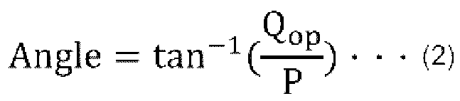
力率角演算部112は、演算した力率角Angleを関数演算部114に入力する。
力率角演算部112は、演算した力率角Angleを関数演算部114に入力する。
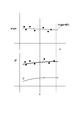
図4は、関数演算部の動作の一例を模式的に表すグラフ図である。
図4に表したように、関数演算部114は、力率角演算部112から入力された力率角Angleを基に、力率角Angleの有効電力値Pに対する関数f(P)を演算する。関数f(P)は、データセットの複数の有効電力値P、無効電力値Q、及び電圧値Vsのそれぞれに対応する複数の力率角Angleを直線近似する一次関数である。
図4に表したように、関数演算部114は、力率角演算部112から入力された力率角Angleを基に、力率角Angleの有効電力値Pに対する関数f(P)を演算する。関数f(P)は、データセットの複数の有効電力値P、無効電力値Q、及び電圧値Vsのそれぞれに対応する複数の力率角Angleを直線近似する一次関数である。
関数演算部114は、換言すれば、複数の力率角Angleに関数f(P)をフィッティングする。力率では、+と-で跳躍が発生する。一方、力率角は、連続である。従って、複数の力率角Angleに関数f(P)をフィッティングする場合には、複数の力率に関数f(P)をフィッティングする場合と比べて、より適切に関数f(P)をフィッティングさせることができる。
一次関数の関数f(P)は、f(P)=A0+A1Pで表すことができる。未知係数A0、A1からなるベクトル ̄Aは、例えば、最小2乗法により、次の(3)式及び(4)式のように求めることができる。なお、(4)式において、「T」は、転置行列を表す。


このように、未知係数のベクトル ̄Aは、有効電力値PのデータからなるΣと、力率角AngleのデータからなるANGLEと、を用いて求めることができる。従って、関数f(P)を構成する力率角の推定値^Angleは、次の(5)式により、計算することができる。

また、関数演算部114は、力率角Angleの関数f(P)を基に、次の(6)式により、力率Pfの推定値^PFを演算するとともに、次の(7)式により、無効電力の推定値^Qを演算する。


関数演算部114は、演算した関数f(P)や各推定値^PF、^Qを表示部116に出力する。
このように、未知係数のベクトル ̄Aは、有効電力値PのデータからなるΣと、力率角AngleのデータからなるANGLEと、を用いて求めることができる。従って、関数f(P)を構成する力率角の推定値^Angleは、次の(5)式により、計算することができる。
また、関数演算部114は、力率角Angleの関数f(P)を基に、次の(6)式により、力率Pfの推定値^PFを演算するとともに、次の(7)式により、無効電力の推定値^Qを演算する。
関数演算部114は、演算した関数f(P)や各推定値^PF、^Qを表示部116に出力する。
表示部116は、図4に表したように、横軸を有効電力値Pとし、縦軸を各推定値^Angle、^PF、^Qとしてプロットしたグラフを解析結果として表示する。なお、表示部116は、ネットワークなどを介して電力系統特性アナライザ100と接続される構成でもよい。表示部116は、必要に応じて設けられ、省略可能である。
このように、表示部116などに表示された各推定値^Angle、^PF、^Qを参照することで、最適無効電力Qopを電力系統4に供給した場合に、定力率制御を行う場合と比べて、分散型電源6の設定力率を改善可能か否かを判断することができる。従って、これらの解析により、分散型電源6の電力変換装置10の力率Pfを事業者側が自立して分析でき、分散型電源6を積極的に最大効率で電力系統4の電源として組み入れることができる。
このように、本実施形態によれば、適切な無効電力を注入するための力率などを推定・解析することができる電力系統特性アナライザ100を提供することができる。
電力系統特性アナライザ100では、推定値演算部104が、拡張カルマンフィルタ(非線形式に対応したカルマンフィルタ)を用いて各推定値^R、^X、^Vrを演算している。これにより、例えば、線形の近似式を用いて電力系統4の系統特性を推定する方法と比べて、電力系統4の系統特性をより適切に推定することができる。
例えば、分散型電源6の設置場所が遠方で、系統インピーダンスの抵抗成分R及びリアクタンス成分Xが大きい場合でも、電力系統4の系統特性をより適切に推定し、連系点LPの電圧変動を抑制することができる。
さらには、工場などの負荷(需要家16)や他の分散型電源(発電機18)が直近にある場合にも、これらの影響を系統特性の変動として推定し、対応する無効電力を演算することができる。例えば、負荷や他の分散型電源が直近にある場合にも、分散型電源6の連系点LPの電圧の変動をより適切に抑制することができる。
また、電力系統特性アナライザ100では、異常値除去部110が、最適無効電力Qopから異常値を除去している。これにより、飛行物体や雲などの通過や、電力系統運用側によるトランスのタップ切替操作などの影響を抑制し、各推定値^Angle、^PF、^Qをより適切に推定することができる。
なお、電力系統特性アナライザ100では、無効電力演算部106の後に異常値除去部110を設け、無効電力演算部106で演算された最適無効電力Qopから異常値を除去している。但し、異常値を除去するタイミングは、これに限定されるものではない。
例えば、データ収集部102と推定値演算部104との間に異常値除去部110を設け、推定値演算部104に入力される有効電力値P、無効電力値Q、及び電圧値Vsから異常値を除去してもよい。あるいは、推定値演算部104と無効電力演算部106との間に異常値除去部110を設け、無効電力演算部106に入力される各推定値^R、^X、^Vrから異常値を除去してもよい。あるいは、力率角演算部112と関数演算部114との間に異常値除去部110を設け、関数演算部114に入力される力率角Angleから異常値を除去してもよい。
このように、異常値除去部110の構成は、関数演算部114で関数f(P)を演算する際に、関数f(P)に異常値が含まれないように、有効電力値P、無効電力値Q、電圧値Vs、各推定値^R、^X、^Vr、最適無効電力Qop、及び力率角Angleのいずれかから異常値を除去可能な任意の構成でよい。
異常値除去部110において異常値を除去する方法は、差分フィルタ108から入力された差分ΔP、ΔQ、ΔVsに基づいて行う方法に限定されるものではない。例えば、ローパスフィルタによって有効電力値P、無効電力値Q、及び電圧値Vsなどの急峻な変動を除去することにより、異常値を除去してもよい。異常値除去部110において異常値を除去する方法は、異常値を適切に除去可能な任意の方法でよい。
電力系統特性アナライザ100では、関数演算部114が、データセットの複数の有効電力値P、無効電力値Q、及び電圧値Vsのそれぞれに対応する複数の力率角Angleを直線近似する一次関数を関数f(P)として演算している。但し、関数f(P)は、一次関数に限ることなく、二次以上の関数でもよい。関数f(P)は、複数の力率角Angleを曲線近似する二次以上の関数でもよい。このように、関数f(P)は、複数の力率角Angleを直線近似又は曲線近似する任意の関数でよい。
関数f(P)を二次以上の関数とした場合には、一次関数とした場合と比べて、関数f(P)を複数の力率角Angleにより適切にフィットさせ、各推定値^Angle、^PF、^Qをより適切に求めることができる。分散型電源6の設定力率を改善可能か否かの判断をより適切に行うことができる。反対に、関数f(P)を一次関数とした場合には、二次以上の関数とした場合と比べて、関数演算部114の演算負荷を軽くすることができる。関数演算部114が演算する関数f(P)の次数は、操作入力などに基づいて変更できるようにしてもよい。
次に、推定値演算部104による拡張カルマンフィルタを用いた各推定値^R、^X、^Vrの演算について説明する。
連系点LPの電圧値Vsは、次の(8)式の非線形式で表すことができる。この非線形式に基づいて拡張カルマンフィルタを適用することにより、各推定値^R、^X、^Vrを演算する。

拡張カルマンフィルタの状態方程式は、次の(9)式で表すことができる。そして、拡張カルマンフィルタの出力方程式は、次の(10)式で表すことができる。


(9)式において、xは、次の(11)式に表すように、電力系統4の系統インピーダンスの抵抗成分R、リアクタンス成分X、及び無限大母線電力系統3の電圧値Vrを成分とする状態ベクトルである。但し、(11)式において、「T」は、転置を表す。

(9)式において、fは、状態ベクトルxの非線形関数である。(9)式において、wは、システムノイズのベクトルである。また、(9)式及び(10)式において、添え字の「k」は、時刻を表す。換言すれば、添え字「k」は、定期的に取得される有効電力値P、無効電力値Q、及び電圧値Vsに対応するデータの順序である。「k-1」は、「k」の1つ前のデータを表す。従って、(9)式は、1つ前の状態ベクトルxから現在の状態ベクトルxを推定することを表している。添え字「k」は、以下の各式においても同様である。
拡張カルマンフィルタの状態方程式は、次の(9)式で表すことができる。そして、拡張カルマンフィルタの出力方程式は、次の(10)式で表すことができる。
(9)式において、xは、次の(11)式に表すように、電力系統4の系統インピーダンスの抵抗成分R、リアクタンス成分X、及び無限大母線電力系統3の電圧値Vrを成分とする状態ベクトルである。但し、(11)式において、「T」は、転置を表す。
(9)式において、fは、状態ベクトルxの非線形関数である。(9)式において、wは、システムノイズのベクトルである。また、(9)式及び(10)式において、添え字の「k」は、時刻を表す。換言すれば、添え字「k」は、定期的に取得される有効電力値P、無効電力値Q、及び電圧値Vsに対応するデータの順序である。「k-1」は、「k」の1つ前のデータを表す。従って、(9)式は、1つ前の状態ベクトルxから現在の状態ベクトルxを推定することを表している。添え字「k」は、以下の各式においても同様である。
(10)式において、zは、電圧値Vsの観測値である。(10)式において、hは、xの非線形関数である。また、(10)式において、vは、観測ノイズである。(10)式は、状態ベクトルxに対する観測値zの反応を表している。この例において、h(x)は、連系点LPの予測電圧値Vsである(h(x)=Vs)。すなわち、観測値zは、連系点LPの電圧値Vsに観測ノイズvを足したものと考えることができる。観測値zは、計測装置22による電圧値Vsの測定値である。
拡張カルマンフィルタは、予測ステップと、更新ステップと、を有する。推定値演算部104は、予測ステップにおいて、次の(12)式により、状態ベクトルxの予測を行う。

(12)式において、xfは、状態ベクトルxの予測値を表す。xaは、更新ステップにおいて更新された状態ベクトルxを表す。このように、この例では、更新後の状態ベクトルxaを、予測後の状態ベクトルxfとして用いる。
(12)式において、xfは、状態ベクトルxの予測値を表す。xaは、更新ステップにおいて更新された状態ベクトルxを表す。このように、この例では、更新後の状態ベクトルxaを、予測後の状態ベクトルxfとして用いる。
推定値演算部104は、この予測後の状態ベクトルxfの各成分を、それぞれ各推定値^R、^X、^Vrとして演算する。すなわち、各推定値^R、^X、^Vrは、換言すれば、更新後の状態ベクトルxaの各成分である。また、推定値演算部104は、状態ベクトルxの初期値を有し、更新ステップが行われていない初期状態においては、この初期値を予測後の状態ベクトルxfとして用いる。
状態ベクトルxの初期値は、一定の値でもよいし、例えば、分散型電源6がソーラーパネルである場合などには、一日分の各推定値^R、^X、^Vrの平均値を算出し、この各推定値^R、^X、^Vrの平均値を次の日の状態ベクトルxの初期値として用いてもよい。推定値演算部104は、各推定値^R、^X、^Vrのそれぞれの所定期間における平均値を算出し、算出した各推定値^R、^X、^Vrの平均値を次の所定期間における状態ベクトルxの初期値とする機能を有してもよい。
推定値演算部104は、予測ステップにおいて、状態ベクトルxの予測を行うとともに、次の(13)式により、共分散行列Pfを予測する。共分散行列Pfは、システムノイズwの影響を考慮した予測後の状態ベクトルxfの誤差共分散行列である。

(13)式において、Jf(x)は、非線形関数fのヤコビアンで定義した行列であり、この例では、次の(14)式に表すように、(1,1,1)の対角行列である。

(13)式において、Pk-1は、1つ前の共分散行列、又は共分散行列の初期値である。(13)式において、Jf(x)Tは、ヤコビアン行列Jf(x)の転置行列である。また、(13)式において、Qk-1は、システムノイズwの共分散行列である。システムノイズwの共分散行列Qk-1は、次の(15)式に表すように、システムノイズw及びその転置行列の内積の期待値である。

推定値演算部104は、データセットに含まれる複数の有効電力値P、無効電力値Q、及び電圧値Vsのうち、次のタイミングで取得された有効電力値P、無効電力値Q、及び電圧値Vsを基に、更新ステップを実行する。推定値演算部104は、更新ステップにおいて、次の有効電力値P、無効電力値Q、及び電圧値Vsを基に、状態ベクトルxを更新する。
(13)式において、Jf(x)は、非線形関数fのヤコビアンで定義した行列であり、この例では、次の(14)式に表すように、(1,1,1)の対角行列である。
(13)式において、Pk-1は、1つ前の共分散行列、又は共分散行列の初期値である。(13)式において、Jf(x)Tは、ヤコビアン行列Jf(x)の転置行列である。また、(13)式において、Qk-1は、システムノイズwの共分散行列である。システムノイズwの共分散行列Qk-1は、次の(15)式に表すように、システムノイズw及びその転置行列の内積の期待値である。
推定値演算部104は、データセットに含まれる複数の有効電力値P、無効電力値Q、及び電圧値Vsのうち、次のタイミングで取得された有効電力値P、無効電力値Q、及び電圧値Vsを基に、更新ステップを実行する。推定値演算部104は、更新ステップにおいて、次の有効電力値P、無効電力値Q、及び電圧値Vsを基に、状態ベクトルxを更新する。
推定値演算部104は、更新ステップにおいて、まず、次のタイミングで取得された有効電力値P、無効電力値Q、及び電圧値Vsの各測定値と共分散行列Pfとを基に、状態ベクトルxを更新するためのカルマンゲインの最適化を行う。カルマンゲインは、次の(16)式によって求められる。

(16)式において、Jh(x)は、非線形関数hのヤコビアンで定義した行列である。この例において、非線形関数h(x)は、連系点LPの電圧値Vsであるから、Jh(x)は、次の(17)式のように表される。

(17)式において、∂Vs/∂R、∂Vs/∂X、∂Vs/∂Vrは、上記の(8)式から、それぞれ次の(18)式、(19)式、(20)式のように表される。



但し、(18)式、(19)式、(20)式において、Bは、次の(21)式、Cは、次の(22)式である。


また、上記の(16)式において、Jh(x)Tは、ヤコビアン行列Jh(x)の転置行列である。(16)式において、Rkは、観測ノイズvの共分散行列である。観測ノイズvの共分散行列Rkは、次の(23)式に表すように、観測ノイズv及びその転置行列の内積の期待値である。

(16)式において、[Jh(x)PfJh(x)T+Rk]-1の部分は、換言すれば、予測誤差(z-h(xf))に対する誤差共分散である。
(16)式において、Jh(x)は、非線形関数hのヤコビアンで定義した行列である。この例において、非線形関数h(x)は、連系点LPの電圧値Vsであるから、Jh(x)は、次の(17)式のように表される。
(17)式において、∂Vs/∂R、∂Vs/∂X、∂Vs/∂Vrは、上記の(8)式から、それぞれ次の(18)式、(19)式、(20)式のように表される。
但し、(18)式、(19)式、(20)式において、Bは、次の(21)式、Cは、次の(22)式である。
また、上記の(16)式において、Jh(x)Tは、ヤコビアン行列Jh(x)の転置行列である。(16)式において、Rkは、観測ノイズvの共分散行列である。観測ノイズvの共分散行列Rkは、次の(23)式に表すように、観測ノイズv及びその転置行列の内積の期待値である。
(16)式において、[Jh(x)PfJh(x)T+Rk]-1の部分は、換言すれば、予測誤差(z-h(xf))に対する誤差共分散である。
推定値演算部104は、更新ステップにおいて、カルマンゲインの最適化を行った後、このカルマンゲインを用い、次の(24)式により、状態ベクトルxを更新する。

(24)式において、h(xf)は、予測後の状態ベクトルxfから(8)式を用いて演算した電圧値Vsの予測値である。すなわち、推定値演算部104は、連系点LPの電圧値Vsの測定値zと、予測後の状態ベクトルxfを用いて演算した連系点LPの電圧値Vsの予測値h(xf)と、を基に、連系点LPの電圧値Vsの予測誤差を求める。推定値演算部104は、測定値zから予測値h(xf)を差し引くことで、予測誤差を求める。
(24)式において、h(xf)は、予測後の状態ベクトルxfから(8)式を用いて演算した電圧値Vsの予測値である。すなわち、推定値演算部104は、連系点LPの電圧値Vsの測定値zと、予測後の状態ベクトルxfを用いて演算した連系点LPの電圧値Vsの予測値h(xf)と、を基に、連系点LPの電圧値Vsの予測誤差を求める。推定値演算部104は、測定値zから予測値h(xf)を差し引くことで、予測誤差を求める。
推定値演算部104は、この予測誤差にカルマンゲインを乗じることにより、状態ベクトルxの補正値を算出し、その補正値を予測後の状態ベクトルxfに加えることにより、更新後の状態ベクトルxaを求める。これにより、予測誤差を考慮して次の状態ベクトルxの予測を行うことができる。
推定値演算部104は、更新ステップにおいて、状態ベクトルxを更新するとともに、次の(25)式により、共分散行列Pも併せて更新する。(25)式に表したように、推定値演算部104は、最適化したカルマンゲインを基に共分散行列Pを更新する。

推定値演算部104は、上記の予測ステップと更新ステップとを繰り返し実行する。これにより、拡張カルマンフィルタによって各推定値^R、^X、^Vrを予測することができる。なお、(25)式において、Iは、単位行列である。
推定値演算部104は、上記の予測ステップと更新ステップとを繰り返し実行する。これにより、拡張カルマンフィルタによって各推定値^R、^X、^Vrを予測することができる。なお、(25)式において、Iは、単位行列である。
次に、本願発明者の行ったシミュレーションの一例について説明する。
図5(a)及び図5(b)は、シミュレーションの一例を模式的に表すグラフ図である。
図5(a)は、有効電力値P及び無効電力値Qの時間的変化を模式的に表す。
図5(b)は、連系点LPの電圧値Vsの時間的変化を模式的に表す。
図5(a)及び図5(b)は、シミュレーションの一例を模式的に表すグラフ図である。
図5(a)は、有効電力値P及び無効電力値Qの時間的変化を模式的に表す。
図5(b)は、連系点LPの電圧値Vsの時間的変化を模式的に表す。
図5(a)及び図5(b)に表したように、シミュレーションでは、有効電力値Pの出力変動を正弦波状とした。図5(b)に表したように、力率-0.94にて定力率制御を行う場合には、連系点LPの電圧値Vsが、有効電力値Pの上昇にともなって減少する。
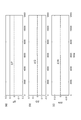
図6(a)~図6(c)は、シミュレーションの一例を模式的に表すグラフ図である。
図6(a)は、有効電力値Pの差分ΔPの時間的変化を模式的に表す。
図6(b)は、無効電力値Qの差分ΔQの時間的変化を模式的に表す。
図6(c)は、電圧値Vsの差分ΔVsの時間的変化を模式的に表す。
図6(a)は、有効電力値Pの差分ΔPの時間的変化を模式的に表す。
図6(b)は、無効電力値Qの差分ΔQの時間的変化を模式的に表す。
図6(c)は、電圧値Vsの差分ΔVsの時間的変化を模式的に表す。
図6(a)~図6(c)に表したように、シミュレーションでは、急峻な変動がない正弦波状の出力変動としてるため、各差分ΔP、ΔQ、ΔVsのそれぞれにも大きな変動は見られない。
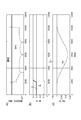
図7(a)~図7(c)は、シミュレーションの一例を模式的に表すグラフ図である。
図7(a)は、予測誤差errの絶対値abs(err)の時間的変化、及び予測誤差errの絶対値abs(err)の閾値abeを模式的に表す。予測誤差errは、推定値演算部104において(z-h(xf))によって演算される予測誤差である。
図7(b)は、系統インピーダンスの抵抗成分Rの推定値^R、及び系統インピーダンスのリアクタンス成分Xの推定値^Xの時間的変化を模式的に表す。
図7(c)は、無限大母線電力系統3の電圧値Vrの推定値^Vr、及び連系点LPの電圧値Vsの時間的変化を模式的に表す。
図7(a)は、予測誤差errの絶対値abs(err)の時間的変化、及び予測誤差errの絶対値abs(err)の閾値abeを模式的に表す。予測誤差errは、推定値演算部104において(z-h(xf))によって演算される予測誤差である。
図7(b)は、系統インピーダンスの抵抗成分Rの推定値^R、及び系統インピーダンスのリアクタンス成分Xの推定値^Xの時間的変化を模式的に表す。
図7(c)は、無限大母線電力系統3の電圧値Vrの推定値^Vr、及び連系点LPの電圧値Vsの時間的変化を模式的に表す。
シミュレーションにおいて、推定値^Rの真値は、0.1である。推定値^Xの真値は、0.4である。推定値^Vrの真値は、1.0である。
図7(a)~図7(c)に表したように、シミュレーションでは、有効電力値Pが立ち上がり始めるまでは、推定値^R及び推定値^Xが初期値(真値ではない)のままである。そして、有効電力値Pが立ち上がり始めると、すぐに真値に収束している。予測誤差errの絶対値abs(err)は、十分に小さい値で済んでいる。例えば、時刻1800付近において、予測誤差errの絶対値abs(err)が大きくなった時に、各推定値^R、^X、^Vrが真値に向けて拡張カルマンフィルタが収束させたことも分かる。
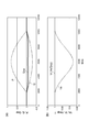
図8(a)及び図8(b)は、シミュレーションの一例を模式的に表すグラフ図である。
図8(a)は、有効電力値P、無効電力値Q、及び最適無効電力Qopの時間的変化を模式的に表す。
図8(b)は、連系点LPの電圧値Vs、無限大母線電力系統3の電圧値Vr、及び最適無効電力Qopから求めた連系点LPの電圧値Vs(Qop)の時間的変化を模式的に表す。
図8(a)は、有効電力値P、無効電力値Q、及び最適無効電力Qopの時間的変化を模式的に表す。
図8(b)は、連系点LPの電圧値Vs、無限大母線電力系統3の電圧値Vr、及び最適無効電力Qopから求めた連系点LPの電圧値Vs(Qop)の時間的変化を模式的に表す。
電圧値Vs(Qop)は、最適無効電力Qopを上記の(8)式に代入して演算した電圧値である。すなわち、電圧値Vs(Qop)は、最適無効電力Qopを電力系統4に供給した時に予測される連系点LPの電圧値である。
図8(a)に表したように、最適無効電力Qopの絶対値は、定力率制御を行った場合の無効電力値Qの絶対値よりも小さい。従って、最適無効電力Qopを出力する制御を行った場合には、定力率制御を行う場合と比べて、力率Pfを改善できることが分かる。
図8(b)に表したように、最適無効電力Qopから求めた連系点LPの電圧値Vs(Qop)は、無限大母線電力系統3の電圧値Vrと実質的に同じである。このように、最適無効電力Qopを出力する制御を行った場合には、定力率制御を行う場合と比べて、連系点LPの電圧の変動をより適切に抑制することができる。
図9(a)~図9(c)は、シミュレーションの一例を模式的に表すグラフ図である。
図9(a)は、定力率制御による無効電力値Q、最適無効電力Qop、及び上記の(7)式によって演算した無効電力の推定値^Qの有効電力値Pに対する変化を模式的に表す。
図9(b)は、定力率制御による力率角Angle、上記の(2)式によって最適無効電力Qopから演算した力率角Angle(Qop)、及び上記の(5)式によって演算した関数f(P)の力率角の推定値^Angleの有効電力値Pに対する変化を模式的に表す。
図9(c)は、定力率制御による力率Pf、最適無効電力Qopから演算した力率Pf(Qop)、及び上記の(6)式によって演算した関数f(P)の力率の推定値^Pfの有効電力値Pに対する変化を模式的に表す。
図9(a)は、定力率制御による無効電力値Q、最適無効電力Qop、及び上記の(7)式によって演算した無効電力の推定値^Qの有効電力値Pに対する変化を模式的に表す。
図9(b)は、定力率制御による力率角Angle、上記の(2)式によって最適無効電力Qopから演算した力率角Angle(Qop)、及び上記の(5)式によって演算した関数f(P)の力率角の推定値^Angleの有効電力値Pに対する変化を模式的に表す。
図9(c)は、定力率制御による力率Pf、最適無効電力Qopから演算した力率Pf(Qop)、及び上記の(6)式によって演算した関数f(P)の力率の推定値^Pfの有効電力値Pに対する変化を模式的に表す。
図9(a)に表したように、推定値^Qは、最適無効電力Qopと実質的に同じである。図9(b)に表したように、推定値^Angleは、最適無効電力Qopから演算した力率角Angle(Qop)と実質的に同じである。図9(c)に表したように、推定値^Pfは、最適無効電力Qopから演算した力率Pf(Qop)と実質的に同じである。
このように、一次関数である関数f(P)から演算した推定値^Angle、^Q、^Pfでも、最適無効電力Qopから演算した場合と実質的に同じ結果を得ることができる。従って、前述のように、表示部116などに表示された各推定値^Angle、^PF、^Qを参照することで、最適無効電力Qopを電力系統4に供給した場合に、定力率制御を行う場合と比べて、分散型電源6の設定力率を改善可能か否かを判断することができる。
図9(a)~図9(c)では、-0.94を定力率制御の力率Pfに設定した例を模式的に表している。有効電力値P、無効電力値Q、及び電圧値Vsから最適無効電力Qopを求めたところ、最適無効電力Qopは、一定ではなく、有効電力値Pにより変化することが分かった。この例において、最適無効電力Qopの平均力率は、-0.995となった。従って、最適無効電力Qopで運転することにより、定力率制御を行う場合と比べて、平均0.055だけ力率が改善されることになる。従って、オーナー側は、力率改善分だけ利益が出ることになる。
図10(a)~図10(f)は、シミュレーションの一例を模式的に表すグラフ図である。
図10(a)は、有効電力値Pの時間的変化を模式的に表す。
図10(b)は、無効電力値Qの時間的変化を模式的に表す。
図10(c)は、電圧値Vsの時間的変化を模式的に表す。
図10(d)は、有効電力値Pの差分ΔPの時間的変化を模式的に表す。
図10(e)は、無効電力値Qの差分ΔQの時間的変化を模式的に表す。
図10(f)は、電圧値Vsの差分ΔVsの時間的変化を模式的に表す。
図10(a)~図10(f)は、有効電力の出力にノイズを含む場合のシミュレーションの一例を模式的に表す。
図10(a)は、有効電力値Pの時間的変化を模式的に表す。
図10(b)は、無効電力値Qの時間的変化を模式的に表す。
図10(c)は、電圧値Vsの時間的変化を模式的に表す。
図10(d)は、有効電力値Pの差分ΔPの時間的変化を模式的に表す。
図10(e)は、無効電力値Qの差分ΔQの時間的変化を模式的に表す。
図10(f)は、電圧値Vsの差分ΔVsの時間的変化を模式的に表す。
図10(a)~図10(f)は、有効電力の出力にノイズを含む場合のシミュレーションの一例を模式的に表す。
図10(a)~図10(f)の時刻t1、t2に表したように、有効電力値Pも無効電力値Qも変化が無く、電圧値Vsのみが急峻に変化している場合には、系統運用側が操作したトランスのタップ切り替えと考えられる。この場合は、系統インピーダンスの抵抗成分R、及び系統インピーダンスのリアクタンス成分Xには変化が無く、無限大母線電力系統3の電圧値Vrのみが変化している。従って、この場合には、無限大母線電力系統3の電圧値Vrに対する推定を重視するようにしてもよい。すなわち、共分散行列の無限大母線電力系統3の電圧値Vr相当の重みを大きくしてもよい。
上記実施形態では、無効電力演算部106が、連系点LPの電圧値Vsを無限大母線電力系統3の電圧値Vrに近付ける(Vs=Vrとする)ための最適無効電力Qopを演算している。無効電力演算部106は、例えば、連系点LPの電圧値Vsを指定値Vsrに近付ける(Vs=Vsrとする)ための無効電力Qnを演算する構成としてもよい。
連系点LPの電圧の指定値Vsrは、例えば、ネットワークなどを介して上位のコントローラから無効電力演算部106に入力される。連系点LPの電圧の指定値Vsrは、例えば、オペレータなどが手動で入力できるようにしてもよい。また、連系点LPの電圧の指定値Vsrは、予め設定された一定の値などでもよい。
図11は、無効電力演算部の動作の一例を模式的に表すグラフ図である。
図11の横軸は、連系点LPの無効電力値Qであり、図11の縦軸は、連系点LPの電圧値Vsである。図4は、無効電力Qnを演算する場合の無効電力演算部の動作の一例を模式的に表す。
図11の横軸は、連系点LPの無効電力値Qであり、図11の縦軸は、連系点LPの電圧値Vsである。図4は、無効電力Qnを演算する場合の無効電力演算部の動作の一例を模式的に表す。
無効電力演算部106は、無効電力Qnを演算する場合、推定値演算部104からの各推定値^R、^X、^Vr、有効電力値P、無効電力値Q、及び電圧値Vsの入力に応じて、図11に表したように、推定値演算部104の演算結果を基に、電圧値Vsの無効電力値Qに対する傾きKを演算する。無効電力演算部106は、次の(26)式により、傾きKを演算する。なお、(26)式において、Bは、(21)式に表したものであり、Cは、(22)式で表したものである。

次回の連系点LPの電圧値をVs(n)、計測装置22で計測された前回の連系点LPの電圧値をVs(n-1)、次回の連系点LPの無効電力値をQn、計測装置22で計測された前回の連系点LPの無効電力値をQn-1とする時、次回の連系点LPの電圧値Vs(n)は、次の(27)式で表すことができる。

従って、次回の連系点LPの電圧値をVs(n)を指定値Vsrとした場合、次回の連系点LPの無効電力Qnは、次の(28)式で表すことができる。

このように、無効電力演算部106は、推定値演算部104から入力された各値を基に、傾きKを演算するとともに、次回の連系点LPの無効電力Qnを演算し、この次回の連系点LPの無効電力Qnを無効電力Qnとして演算する。
次回の連系点LPの電圧値をVs(n)、計測装置22で計測された前回の連系点LPの電圧値をVs(n-1)、次回の連系点LPの無効電力値をQn、計測装置22で計測された前回の連系点LPの無効電力値をQn-1とする時、次回の連系点LPの電圧値Vs(n)は、次の(27)式で表すことができる。
従って、次回の連系点LPの電圧値をVs(n)を指定値Vsrとした場合、次回の連系点LPの無効電力Qnは、次の(28)式で表すことができる。
このように、無効電力演算部106は、推定値演算部104から入力された各値を基に、傾きKを演算するとともに、次回の連系点LPの無効電力Qnを演算し、この次回の連系点LPの無効電力Qnを無効電力Qnとして演算する。
この場合には、所望の指定値Vsrに基づく無効電力Qnを電力系統4に供給した場合に、定力率制御を行う場合と比べて、分散型電源6の設定力率を改善可能か否かを判断することができる。
例えば、最適無効電力Qopに基づく解析と、無効電力Qnに基づく解析と、を任意に切り替えられるようにしてもよい。これにより、電力系統特性アナライザ100の利便性をより向上させることができる。
以上、具体例を参照しつつ、本発明の実施の形態について説明した。しかし、本発明の実施形態は、これらの具体例に限定されるものではない。例えば、分散型電源システム2及び電力系統特性アナライザ100に含まれる各要素の具体的な構成に関しては、当業者が公知の範囲から適宜選択することにより本発明を同様に実施し、同様の効果を得ることができる限り、本発明の範囲に包含される。
また、各具体例のいずれか2つ以上の要素を技術的に可能な範囲で組み合わせたものも、本発明の要旨を包含する限り本発明の範囲に含まれる。
また、各具体例のいずれか2つ以上の要素を技術的に可能な範囲で組み合わせたものも、本発明の要旨を包含する限り本発明の範囲に含まれる。
その他、本発明の実施の形態として上述した分散型電源システム2及び電力系統特性アナライザ100を基にして、当業者が適宜設計変更して実施し得る全ての分散型電源システム及び電力系統特性アナライザも、本発明の要旨を包含する限り、本発明の範囲に属する。
その他、本発明の思想の範疇において、当業者であれば、各種の変更例及び修正例に想到し得るものであり、それら変更例及び修正例についても本発明の範囲に属するものと了解される。
本発明のいくつかの実施形態を説明したが、これらの実施形態は、例として提示したものであり、発明の範囲を限定することは意図していない。これら新規な実施形態は、その他の様々な形態で実施されることが可能であり、発明の要旨を逸脱しない範囲で、種々の省略、置き換え、変更を行うことができる。これら実施形態やその変形は、発明の範囲や要旨に含まれるとともに、請求の範囲に記載された発明とその均等の範囲に含まれる。
Claims (8)
- 分散型電源の電力を無限大母線電力系統につながる電力系統に対応した交流電力に変換し、変換後の交流電力を前記電力系統に供給することにより、前記分散型電源を前記電力系統と連系させる電力変換装置とともに用いられ、前記電力系統の系統特性の解析を行う電力系統特性アナライザであって、
前記電力変換装置の前記電力系統との連系点の有効電力値と、前記連系点の無効電力値と、前記連系点の電圧値と、を定期的に取得することにより、所定期間において定期的に取得した複数の前記有効電力値、前記無効電力値、及び前記電圧値からなるデータセットを収集するデータ収集部と、
非線形式に対応したカルマンフィルタを用いることにより、前記データセットに含まれる前記有効電力値、前記無効電力値、及び前記電圧値を基に、前記電力系統の系統インピーダンスの抵抗成分の推定値と、前記系統インピーダンスのリアクタンス成分の推定値と、前記無限大母線電力系統の電圧値の推定値と、を演算する推定値演算部と、
前記系統インピーダンスの抵抗成分の推定値と、前記系統インピーダンスのリアクタンス成分の推定値と、前記無限大母線電力系統の電圧値の推定値と、を基に、前記電力系統に供給する無効電力を演算する無効電力演算部と、
前記無効電力を基に力率角を演算する力率角演算部と、
前記データセットの複数の前記有効電力値、前記無効電力値、及び前記電圧値のそれぞれに対応する複数の前記力率角を直線近似又は曲線近似する関数を演算する関数演算部と、
を備えた電力系統特性アナライザ。 - 前記関数演算部は、前記力率角の前記関数を基に、力率の推定値と、無効電力の推定値と、をさらに演算する請求項1記載の電力系統特性アナライザ。
- 前記関数演算部で前記関数を演算する際に、前記関数に異常値が含まれないように、前記データセットに含まれる前記有効電力値、前記無効電力値、前記電圧値、前記推定値演算部で演算された前記抵抗成分の推定値、前記リアクタンス成分の推定値、前記無限大母線電力系統の電圧値の推定値、前記無効電力演算部で演算された前記無効電力、及び前記力率角演算部で演算された前記力率角のいずれかから異常値を除去する異常値除去部を、さらに備えた請求項1又は2に記載の電力系統特性アナライザ。
- 前記無効電力演算部は、前記連系点の電圧値を前記無限大母線電力系統の電圧値に近付ける最適無効電力を演算する請求項1~3のいずれか1つに記載の電力系統特性アナライザ。
- 前記推定値演算部は、前記非線形式に対応したカルマンフィルタとして拡張カルマンフィルタを用いる請求項1~4のいずれか1つに記載の電力系統特性アナライザ。
- 前記推定値演算部は、前記系統インピーダンスの抵抗成分、前記系統インピーダンスのリアクタンス成分、及び前記無限大母線電力系統の電圧値を成分とする状態ベクトルの予測を行い、予測後の前記状態ベクトルの各成分を、それぞれ前記電力系統の系統インピーダンスの抵抗成分の推定値、前記系統インピーダンスのリアクタンス成分の推定値、及び前記無限大母線電力系統の電圧値の推定値として演算するとともに、次に取得された前記有効電力値、前記無効電力値、及び前記連系点の電圧値を基に、前記状態ベクトルを更新する請求項5記載の電力系統特性アナライザ。
- 前記推定値演算部は、更新後の前記状態ベクトルを、予測後の前記状態ベクトルとして用いる請求項6記載の電力系統特性アナライザ。
- 前記推定値演算部は、
前記状態ベクトルの予測を行うとともに、予測後の前記状態ベクトルの誤差に関する共分散行列の予測を行い、
取得した前記有効電力値、前記無効電力値、及び前記連系点の電圧値の各測定値と前記共分散行列とを基に、前記状態ベクトルを更新するためのカルマンゲインの最適化を行い、
前記連系点の電圧値の測定値と、予測後の前記状態ベクトルを用いて演算した前記連系点の電圧値の予測値と、を基に、前記連系点の電圧値の予測誤差を求め、
最適化した前記カルマンゲインと前記予測誤差とを基に前記状態ベクトルを更新するとともに、最適化した前記カルマンゲインを基に前記共分散行列を更新する請求項6又は7記載の電力系統特性アナライザ。
Priority Applications (2)
| Application Number | Priority Date | Filing Date | Title |
|---|---|---|---|
| JP2019557642A JP6762078B1 (ja) | 2019-07-23 | 2019-07-23 | 電力系統特性アナライザ |
| PCT/JP2019/028887 WO2021014580A1 (ja) | 2019-07-23 | 2019-07-23 | 電力系統特性アナライザ |
Applications Claiming Priority (1)
| Application Number | Priority Date | Filing Date | Title |
|---|---|---|---|
| PCT/JP2019/028887 WO2021014580A1 (ja) | 2019-07-23 | 2019-07-23 | 電力系統特性アナライザ |
Publications (1)
| Publication Number | Publication Date |
|---|---|
| WO2021014580A1 true WO2021014580A1 (ja) | 2021-01-28 |
Family
ID=72614745
Family Applications (1)
| Application Number | Title | Priority Date | Filing Date |
|---|---|---|---|
| PCT/JP2019/028887 Ceased WO2021014580A1 (ja) | 2019-07-23 | 2019-07-23 | 電力系統特性アナライザ |
Country Status (2)
| Country | Link |
|---|---|
| JP (1) | JP6762078B1 (ja) |
| WO (1) | WO2021014580A1 (ja) |
Cited By (1)
| Publication number | Priority date | Publication date | Assignee | Title |
|---|---|---|---|---|
| JP2023549742A (ja) * | 2020-11-24 | 2023-11-29 | レモニ エー/エス | 地下電力ケーブルの絶縁欠陥を検出するためのシステム及び方法 |
Citations (4)
| Publication number | Priority date | Publication date | Assignee | Title |
|---|---|---|---|---|
| JP2007300784A (ja) * | 2006-04-06 | 2007-11-15 | Tokyo Electric Power Co Inc:The | 分散型電源 |
| JP2017063525A (ja) * | 2015-09-24 | 2017-03-30 | 東芝三菱電機産業システム株式会社 | 分散型電源システムの制御装置および制御方法 |
| JP2017189028A (ja) * | 2016-04-06 | 2017-10-12 | 富士電機株式会社 | 分散型電源の制御方法及び制御装置 |
| JP2017221040A (ja) * | 2016-06-08 | 2017-12-14 | 株式会社東芝 | 配電系統監視装置 |
Family Cites Families (2)
| Publication number | Priority date | Publication date | Assignee | Title |
|---|---|---|---|---|
| CN103166232B (zh) * | 2013-02-04 | 2015-03-04 | 中冶南方工程技术有限公司 | 基于卡尔曼滤波的无功补偿装置状态估计方法 |
| WO2014199502A1 (ja) * | 2013-06-14 | 2014-12-18 | 株式会社 日立製作所 | 電力系統制御装置、システム及び方法 |
-
2019
- 2019-07-23 WO PCT/JP2019/028887 patent/WO2021014580A1/ja not_active Ceased
- 2019-07-23 JP JP2019557642A patent/JP6762078B1/ja active Active
Patent Citations (4)
| Publication number | Priority date | Publication date | Assignee | Title |
|---|---|---|---|---|
| JP2007300784A (ja) * | 2006-04-06 | 2007-11-15 | Tokyo Electric Power Co Inc:The | 分散型電源 |
| JP2017063525A (ja) * | 2015-09-24 | 2017-03-30 | 東芝三菱電機産業システム株式会社 | 分散型電源システムの制御装置および制御方法 |
| JP2017189028A (ja) * | 2016-04-06 | 2017-10-12 | 富士電機株式会社 | 分散型電源の制御方法及び制御装置 |
| JP2017221040A (ja) * | 2016-06-08 | 2017-12-14 | 株式会社東芝 | 配電系統監視装置 |
Cited By (1)
| Publication number | Priority date | Publication date | Assignee | Title |
|---|---|---|---|---|
| JP2023549742A (ja) * | 2020-11-24 | 2023-11-29 | レモニ エー/エス | 地下電力ケーブルの絶縁欠陥を検出するためのシステム及び方法 |
Also Published As
| Publication number | Publication date |
|---|---|
| JPWO2021014580A1 (ja) | 2021-09-13 |
| JP6762078B1 (ja) | 2020-09-30 |
Similar Documents
| Publication | Publication Date | Title |
|---|---|---|
| Saxena et al. | An MPC based algorithm for a multipurpose grid integrated solar PV system with enhanced power quality and PCC voltage assist | |
| CA3007781C (en) | Electrical systems and related frequency regulation methods | |
| JP6059757B2 (ja) | 系統電圧抑制制御装置及び系統電圧抑制制御方法 | |
| Metry et al. | Sensorless current model predictive control for maximum power point tracking of single-phase subMultilevel inverter for photovoltaic systems | |
| WO2017103697A1 (en) | Power sharing for dc microgrids | |
| Konstantinou et al. | Estimation methods and sensor reduction in modular multilevel converters: A review | |
| Shadmand et al. | Model predictive control of grid-tied photovoltaic systems: Maximum power point tracking and decoupled power control | |
| KR101124014B1 (ko) | 발전 시스템의 전력 품질 제어 장치 및 방법 | |
| CN119231588A (zh) | 基于分布式储能系统的储能设备并网控制方法及装置 | |
| Singh et al. | Single-phase single-stage grid tied solar PV system with active power filtering using power balance theory | |
| Mohanraj et al. | A unified power quality conditioner for power quality improvement in distributed generation network using adaptive distributed power balanced control (ADPBC) | |
| JP6762078B1 (ja) | 電力系統特性アナライザ | |
| JP6873587B1 (ja) | 電力変換装置及び分散型電源システム | |
| CN114447994B (zh) | 适用于新能源智能并网柜的无功补偿并网方法及系统 | |
| JP7058056B2 (ja) | 電力変換装置及び分散型電源システム | |
| Mahmud et al. | Nonlinear partial feedback linearizing output feedback control of islanded DC microgrids | |
| JP6842815B1 (ja) | 電力変換装置及び分散型電源システム | |
| Pragathi et al. | Power quality improvement for grid interconnected solar PV system using neural network control algorithm | |
| Latham et al. | Output feedback control of a single phase voltage source inverter utilizing a variable structure observer | |
| Chai et al. | Dual-model predictive control for cascaded h-bridge multilevel active rectifier with dc voltage balancing in a solid-state transformer | |
| Wang et al. | Analysis of harmonic interactions between DG inverters and polluted grids | |
| Kumar et al. | An integration of solar photovoltaic generation to three-phase utility using adaptive control algorithm | |
| Datta et al. | Minimal-order observer-based coordinated control method for isolated power utility connected multiple photovoltaic systems to reduce frequency deviations | |
| Abid et al. | Model-free predictive current control for voltage source inverter: a comparative investigation | |
| Lopez-Garcia et al. | Neural control for battery integration to DC microgrids |
Legal Events
| Date | Code | Title | Description |
|---|---|---|---|
| ENP | Entry into the national phase |
Ref document number: 2019557642 Country of ref document: JP Kind code of ref document: A |
|
| 121 | Ep: the epo has been informed by wipo that ep was designated in this application |
Ref document number: 19938907 Country of ref document: EP Kind code of ref document: A1 |
|
| NENP | Non-entry into the national phase |
Ref country code: DE |
|
| 122 | Ep: pct application non-entry in european phase |
Ref document number: 19938907 Country of ref document: EP Kind code of ref document: A1 |