WO2019012887A1 - 図形パターンの形状補正装置および形状補正方法 - Google Patents
図形パターンの形状補正装置および形状補正方法 Download PDFInfo
- Publication number
- WO2019012887A1 WO2019012887A1 PCT/JP2018/022296 JP2018022296W WO2019012887A1 WO 2019012887 A1 WO2019012887 A1 WO 2019012887A1 JP 2018022296 W JP2018022296 W JP 2018022296W WO 2019012887 A1 WO2019012887 A1 WO 2019012887A1
- Authority
- WO
- WIPO (PCT)
- Prior art keywords
- unit
- end point
- pattern
- graphic
- point
- Prior art date
- Legal status (The legal status is an assumption and is not a legal conclusion. Google has not performed a legal analysis and makes no representation as to the accuracy of the status listed.)
- Ceased
Links
Images




























Classifications
-
- G—PHYSICS
- G03—PHOTOGRAPHY; CINEMATOGRAPHY; ANALOGOUS TECHNIQUES USING WAVES OTHER THAN OPTICAL WAVES; ELECTROGRAPHY; HOLOGRAPHY
- G03F—PHOTOMECHANICAL PRODUCTION OF TEXTURED OR PATTERNED SURFACES, e.g. FOR PRINTING, FOR PROCESSING OF SEMICONDUCTOR DEVICES; MATERIALS THEREFOR; ORIGINALS THEREFOR; APPARATUS SPECIALLY ADAPTED THEREFOR
- G03F1/00—Originals for photomechanical production of textured or patterned surfaces, e.g., masks, photo-masks, reticles; Mask blanks or pellicles therefor; Containers specially adapted therefor; Preparation thereof
- G03F1/36—Masks having proximity correction features; Preparation thereof, e.g. optical proximity correction [OPC] design processes
-
- G—PHYSICS
- G03—PHOTOGRAPHY; CINEMATOGRAPHY; ANALOGOUS TECHNIQUES USING WAVES OTHER THAN OPTICAL WAVES; ELECTROGRAPHY; HOLOGRAPHY
- G03F—PHOTOMECHANICAL PRODUCTION OF TEXTURED OR PATTERNED SURFACES, e.g. FOR PRINTING, FOR PROCESSING OF SEMICONDUCTOR DEVICES; MATERIALS THEREFOR; ORIGINALS THEREFOR; APPARATUS SPECIALLY ADAPTED THEREFOR
- G03F7/00—Photomechanical, e.g. photolithographic, production of textured or patterned surfaces, e.g. printing surfaces; Materials therefor, e.g. comprising photoresists; Apparatus specially adapted therefor
- G03F7/20—Exposure; Apparatus therefor
-
- G—PHYSICS
- G06—COMPUTING OR CALCULATING; COUNTING
- G06F—ELECTRIC DIGITAL DATA PROCESSING
- G06F30/00—Computer-aided design [CAD]
-
- H—ELECTRICITY
- H10—SEMICONDUCTOR DEVICES; ELECTRIC SOLID-STATE DEVICES NOT OTHERWISE PROVIDED FOR
- H10P—GENERIC PROCESSES OR APPARATUS FOR THE MANUFACTURE OR TREATMENT OF DEVICES COVERED BY CLASS H10
- H10P76/00—Manufacture or treatment of masks on semiconductor bodies, e.g. by lithography or photolithography
Definitions
- the present invention relates to a shape correction apparatus and shape correction method for a graphic pattern, and more particularly to a technology for correcting the shape of a graphic pattern formed on a substrate through a lithography process.
- fine patterns are formed on a physical substrate through a lithography process involving drawing using light or an electron beam.
- a method has been taken to form
- a fine mask pattern is designed using a computer, and the resist layer formed on the substrate is exposed based on the data of the mask pattern obtained, developed, and then the remaining resist layer is masked. Etching is performed to form a fine pattern on the substrate.
- the lithography process includes the steps of exposure, development, and etching, so the actual figure pattern finally formed on the substrate does not exactly match the original figure pattern used in the exposure step. It is for.
- drawing on the resist layer is performed by light or electron beam.
- the exposure region actually drawn on the resist layer by the proximity effect is the original figure It is known that the area is slightly larger than the pattern.
- PE Proximity Effect
- a process of manufacturing a semiconductor device including a lithography process after designing a desired original figure pattern on a computer, the lithography process using this original figure pattern is simulated on a computer, and an actual substrate is obtained. A procedure is performed to estimate the shape of the real figure pattern that will be formed on top. Then, based on the shape (dimension) of the actual figure pattern obtained as a result of simulation, correction is performed on the shape (dimension) of the original figure pattern as necessary, and the correction figure pattern obtained by this correction is actually used.
- the lithography process will be performed to produce the actual semiconductor device.
- Patent Document 1 a feature factor characterizing the layout of the original figure pattern and a control factor affecting the dimension of the resist pattern formed on the substrate by the lithography process are used as the input layer.
- a method of performing high-precision simulation using a neural network is disclosed.
- Patent Document 2 discloses a method of enhancing the accuracy of simulation using two sets of neural networks
- Patent Document 3 is suitable for extracting feature quantities from a pattern of a photomask. It is disclosed a method of improving simulation accuracy by setting various extraction parameters.
- JP 2008-122929 A JP, 2010-044101, A JP, 2010-156866, A
- an evaluation point is set at a predetermined position on an original figure pattern, and based on a feature amount indicating a feature around the evaluation point, the deviation amount on the actual figure pattern for the evaluation point
- a corrected figure pattern is created by obtaining (process bias) by simulation and performing correction according to the amount of deviation. Therefore, it is very important to set an appropriate number of evaluation points at appropriate positions on the original graphic pattern.
- the density of the evaluation points is increased to set a large number of evaluation points, the accuracy of the simulation can be improved and more accurate correction can be performed.
- the computational load on the simulation increases, and the time to complete the simulation increases. For this reason, it is desired to perform efficient evaluation point setting that can reduce the calculation load as much as possible while maintaining simulation accuracy sufficient for practical use.
- the original figure pattern in forming a real figure pattern on a real substrate by a lithography process based on the original figure pattern, the original figure pattern is formed so that the real figure pattern matches the original figure pattern.
- a figure pattern shape correction apparatus for correcting a shape and creating a corrected figure pattern actually used in a lithography process,
- An evaluation point setting unit for setting an evaluation point at a predetermined position on an outline indicating the boundary between the inside and the outside for each unit graphic forming the original graphic pattern;
- a feature amount extraction unit for extracting feature amounts indicating features around evaluation points for a source figure pattern;
- a bias estimation unit for estimating a process bias indicating an amount of deviation between the position on the original figure pattern of the evaluation point and the position on the actual figure pattern based on the feature amount;
- a pattern correction unit that generates a corrected figure pattern by performing correction on the original figure pattern based on the estimated value of the process bias output from the bias estimation unit;
- Provide The evaluation point setting unit A unit graphic input unit for inputting individual unit graphics consist
- An overlapping segment portion of the searched overlapping vector pairs is searched from the set of divided figure vectors, arranged on overlapping sides of a pair of adjacent polygons adjacent to each other and directed in the opposite direction to each other.
- a unit figure vector definition unit that defines a plurality of unit figure vectors arranged along the contour of the unit figure by the remaining vectors.
- a normal end point definition unit which defines an end point at each of starting point positions of individual unit graphic vectors; Between two ordinary end points arranged adjacent to each other on the contour line of each unit graphic, an evaluation point definition unit which defines an evaluation point, and A replenishment end point definition unit which searches for an intermediate normal end point, which is a normal end point not constituting a polygon vertex, and additionally defines a replenishment end point at the same position as the searched intermediate normal end point for each unit figure;
- the pattern correction unit For each evaluation point, the normal end point or replenishment end point adjacent to one side of the evaluation point along the contour of the unit figure is the first end point, and the normal end point or replenishment end point adjacent to the other side is the second
- a movement process in which a contour line segment as an end point of is defined, and a contour line segment for each evaluation point is moved in a direction orthogonal to the contour line segment by a correction amount according to the estimated value of the process bias of the evaluation point Contour line segment movement processing unit for performing If the intermediate normal end point and the replenishment
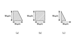
- the unit graphic division unit divides the unit graphic to form a trapezoidal divided graphic.
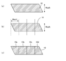
- the unit graphic input unit inputs an elongated strip unit graphic extending along a predetermined longitudinal axis and having linear upper and lower sides parallel to each other, A plurality of divided figures arranged one-dimensionally along the longitudinal axis by dividing the strip-shaped unit figure by a plurality of dividing lines arranged at predetermined intervals along the longitudinal axis.
- a plurality of unit graphic division units arrange a plurality of horizontal division lines parallel to the X axis at predetermined intervals in the Y axis direction, and divide the unit graphic by the plurality of horizontal division lines, thereby extending a plurality of elongated shapes in the X axis direction
- the unit figure dividing unit has a function of setting the beam maximum forming size of the drawing apparatus used in the lithography process, and sets the arrangement interval of the dividing lines used for dividing the unit figure to the beam maximum forming size or less. is there.
- the divided figure vector definition unit numbers the first vertex to the Kth vertex in the order of clockwise or counterclockwise along the outline to each vertex of the divided figure consisting of K square, and the k th vertex
- the divided figure vector of the division figure is defined.
- the evaluation point is defined at the middle point position of two normal end points disposed adjacent to each other on the contour line of the unit graphic.
- the contour line segment expansion / contraction unit separates one corner normal end point into a first moving end point and a second moving end point by moving processing
- the first moving end point is one end point.
- the intersection of the straight line including the post-movement contour line segment and the straight line including the second post-movement contour line segment having the second moving end point as one end point is determined, and the intersection point is set as a new corner normal end point,
- the extension and contraction processing is performed such that one end point becomes the new corner normal end point with respect to the after-moving outline line segment and the second after-moving outline line segment.
- the evaluation point setting unit further includes an end point reconstruction unit for performing reconstruction to correct the number or position of the normal end points defined on the outline of the unit graphic by the normal end point definition unit;
- the evaluation point definition unit defines an evaluation point based on the normal end points obtained by the above reconstruction.
- the end point reconstructing unit is configured to perform normal end point reconstruction by an end point removing process of removing some or all of the intermediate normal end points for some or all unit graphics.
- a twelfth aspect of the present invention is the shape correction apparatus for a graphic pattern according to the eleventh aspect described above,
- the end point reconstructing unit is configured to arrange a total of N normal end points defined for one outline of one unit graphic in the order of the first normal end point T (1) to the Nth Of the n-th normal end point T (n) and a normal end point T (n-m) not to be removed located immediately before the n-th normal end point T (n) (where m is a natural number)
- the distance to T (n ⁇ m + N) is L1
- L2 be the distance between the first normal end point T (1) and so on)
- N N ⁇ 1
- a fourteenth aspect of the present invention is the shape correction apparatus for a graphic pattern according to the tenth aspect described above,
- the end point reconstruction unit reconstructs the normal end points by an end point rearrangement process in which intermediate normal end points are once removed for some outlines, and new intermediate normal ends are placed on each side of the partial outlines. It is intended to
- the end point reconstruction unit performs end point rearrangement processing by repositioning the intermediate normal end points at predetermined intervals on each side of the specific outline after removing the intermediate normal end point for the specific outline.
- the end point reconstruction unit performs end point removal processing by the shape correction device for graphic patterns according to the eleventh to thirteenth aspects described above, and end point rearrangement using the shape correction device for graphic patterns according to the fourteenth or fifteenth aspect described above Processing, and has the function of selectively executing each contour of the unit figure, End points are reconstructed by the above-mentioned end point removal processing for ordinary endpoints on a regular figure surrounded by unit figure vectors around the forward direction, and are enclosed by unit figure vectors around the reverse direction opposite to the forward direction. With respect to the normal end points on the anti-graphic, end point reconstruction is performed by the above end point rearrangement processing.
- the feature amount extraction unit has a function of extracting, for the corrected figure pattern created by the pattern correction unit, a feature amount indicating a feature around an evaluation point on the corrected figure pattern.
- the bias estimation unit has a function of estimating a process bias indicating the amount of deviation between the position on the corrected figure pattern of the evaluation point and the position on the actual figure pattern based on the feature amount,
- the pattern correction unit has a function of creating a new corrected graphic pattern by further correcting the corrected graphic pattern based on the estimated value of the process bias output from the bias estimation unit, The correction on the corrected figure pattern is repeatedly performed.
- an evaluation point setting unit or pattern correction unit included in the shape correction device for a graphic pattern or the shape correction device for the graphic pattern according to the first to eighteenth aspects is provided. It is configured by incorporating a program into a computer.
- the real figure pattern matches the original figure pattern
- An evaluation point setting step in which the computer sets an evaluation point at a predetermined position on an outline indicating the boundary between the inside and the outside for each unit graphic forming the original graphic pattern;
- a feature amount extraction stage in which a computer extracts feature amounts indicating features around evaluation points for the original figure pattern;
- a bias estimation step in which a computer estimates a process bias indicating a deviation between a position on an original figure pattern of an evaluation point and a position on a real figure pattern based on the feature amount;
- a pattern correction step in which a computer generates a corrected figure pattern by correcting the original figure pattern based on the estimated value of the process bias obtained by the bias estimation step;
- Have The evaluation point setting stage is A unit figure input step
- An overlapping segment portion of the searched overlapping vector pairs is searched from the set of divided figure vectors, arranged on overlapping sides of a pair of adjacent polygons adjacent to each other and directed in the opposite direction to each other.
- a normal end point defining step that defines an end point at each of starting point positions of individual unit graphic vectors;
- Have The pattern correction stage is For each evaluation point, the normal end point or replenishment end point adjacent to one side of the evaluation point along the contour of the unit figure is the first end point, and the normal end point or replenishment end point adjacent to the other side is the second
- a movement process in which a contour line segment as an end point of is defined, and a contour line segment for each evaluation point is moved in a direction orthogonal to the contour line segment by a correction amount according to the estimated value of the process bias of the evaluation point Contour line segment moving step to If the intermediate normal end point
- a twenty-first aspect of the present invention is the shape correction method for a graphic pattern according to the twentieth aspect described above,
- the evaluation point setting step further includes an end point reconstruction step for performing a reconstruction that corrects the number or position with respect to the normal end points defined by the normal end point definition step;
- evaluation points are defined based on the normal end points obtained by reconstruction.
- the shape correction apparatus and shape correction method of a figure pattern according to the present invention, after the unit figure constituting the original figure pattern is divided into polygons, end points are defined based on the vertex position of this polygon, An evaluation point is defined for each of the contour line segments connecting two adjacent end points, and the position can be corrected for each of the contour line segments. Therefore, when performing correction on the original graphic pattern, it is possible to perform efficient evaluation point setting that can reduce the calculation load as much as possible while maintaining simulation accuracy sufficient for practical use. Also, if an embodiment is further performed in which the end point is further reconstructed with respect to the end point defined on the basis of the vertex position of the polygon, the number and position of the end point are corrected, and more efficient evaluation point setting is performed. It becomes possible.
- FIG. 1 is a block diagram showing a configuration of a figure pattern shape correction apparatus 100 according to a prior application invention and a basic embodiment of the present invention. It is a top view which shows an example in which the difference in shape arose between the original figure pattern and the real figure pattern. In the example shown in FIG. 2, it is a top view which shows the example of a setting of each evaluation point, and the process bias which arises in each evaluation point. It is a flowchart which shows the design and manufacturing process of a product using the shape correction apparatus 100 of the figure pattern shown in FIG. It is a top view which shows the concept which grasps
- FIG. 10 It is a figure which shows the edge length density map M2 produced based on the original figure pattern 10 shown in FIG. It is a top view which shows the original figure pattern 10 containing the information of dose amount. It is a figure which shows the dose density map M3 created based on the dose-added original figure pattern 10 shown in FIG. It is a top view which shows the procedure which produces the k-th hierarchical image Pk by performing the filter processing using Gaussian filter GF33 to the k-th preparatory image Qk. It is a top view which shows the k-th hierarchy image Pk obtained by the filter process shown in FIG. It is a top view which shows the example of the image processing filter utilized for the filter processing shown in FIG.
- FIG. 10 is a plan view showing a procedure for creating an image pyramid PP composed of n kinds of hierarchical images P1 to Pn in the image pyramid creating unit 122 shown in FIG. 1.
- FIG. 10 is a plan view showing a procedure for creating an image pyramid PD composed of n kinds of difference images D1 to Dn in the image pyramid creating unit 122 shown in FIG. 1.
- FIG. 27 is a view showing a specific example of the activation function f ( ⁇ ) shown in FIG. 26.
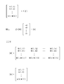
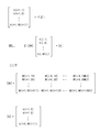
- FIG. 26 is a diagram showing arithmetic expressions for obtaining respective values of the second hidden layer to the Nth hidden layer in the diagram shown in FIG. 25. It is a figure which shows the computing equation which calculates
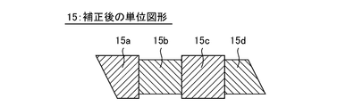
- FIG. 37 is a plan view showing an example of an exposure process based on the unit figure 15 after correction shown in FIG. 36.
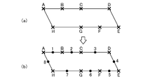
- FIG. 32 shows an example in which processing by the divided figure vector definition unit 113, the unit figure vector definition unit 114, and the normal end point definition unit 115 shown in FIG. 32 is performed on the parallelogram unit figure 10 shown in FIG. It is a top view shown.
- FIG. 32 shows an example in which processing by unit graphic division unit 112, divided graphic vector definition unit 113, unit graphic vector definition unit 114, and normal end point definition unit 115 shown in FIG. It is a top view.
- FIG. 33 is a schematic view (FIG.
- FIG. 33 is a schematic view (FIG.
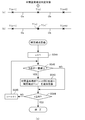
- FIG. (A) and a flow chart (FIG. (B)) showing a procedure in the case of adopting the four-point end point removal process as the end point reconstruction process by the end point reconstruction unit 116 shown in FIG.
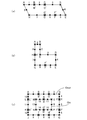
- FIG. 43 is a plan view showing an example in which evaluation points 1 to 8 are defined on the parallelogram type unit graphic 10 after the end point reconstruction shown in FIG. 42 (b) by the evaluation point definition unit 117 shown in FIG.
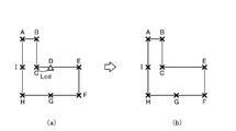
- FIG. 43 is a plan view showing an example in which evaluation points 1 to 8 are defined on the L-shaped unit graphic 10 after the end point reconstruction shown in FIG. 43 (b) by the evaluation point definition unit 117 shown in FIG.
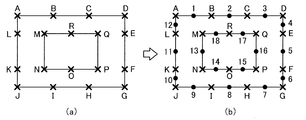
- FIG. 37 is a plan view showing an example in which evaluation points 1 to 18 are defined on the B-shaped unit graphic 10 after the end point reconstruction shown in FIG. 47 (b) by the evaluation point definition unit 117 shown in FIG.
- FIG. 49 is a plan view showing an example in which replenishment end points are defined on each unit figure shown in FIG. 48 (b), FIG.
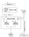
- FIG. 2 is a block diagram showing a pattern correction unit 140 in a figure pattern shape correction apparatus 100 (see FIG. 1) according to a basic embodiment of the present invention and components related thereto.
- FIG. 52 is an enlarged plan view showing each end point and each evaluation point defined on the L-shaped unit graphic shown in FIG. 51 (b).
- FIG. 55 is a plan view showing a state in which contour line segment movement processing has been performed on an L-shaped unit graphic 10 shown in FIG. 54 by the contour line segment movement processing unit 141 shown in FIG. 53;
- FIG. 55 is a plan view showing a state in which contour line segment addition processing has been performed on the L-shaped unit graphic after movement processing shown in FIG. 56 by the contour line segment addition processing unit 142 shown in FIG. 53;
- FIG. 60 is a plan view showing a state in which the contour line segment expansion and contraction processing has been performed on the L-shaped unit graphic after the addition processing shown in FIG.
- FIG. 57 by the contour line segment expansion and contraction processing unit 143 shown in FIG. 58 is a plan view showing a state in which the contour line segment of the L-shaped unit graphic after the stretching process shown in FIG. 58 has been subjected to processing of correcting the position of the evaluation point by the contour line segment stretching processing unit 143 shown in FIG. is there.
- it is a top view showing the merit which divides a unit figure into a polygon and defines an end point on the basis of the vertex position of this polygon. It is a top view which shows the merit which defines a replenishment end point.
- FIG. 59 is a plan view showing a disadvantage in the case where end point reconstruction is not performed in the example shown in FIG. 58.
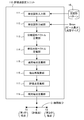
- the shape correction apparatus 100 of the figure pattern includes an evaluation point setting unit 110, a feature extraction unit 120, a bias estimation unit 130, and a pattern correction unit 140.
- three units of the evaluation point setting unit 110, the feature value extraction unit 120, and the bias estimation unit 130 constitute the figure pattern shape estimation apparatus 100 'according to the prior invention, and the figure according to the prior invention
- the pattern shape correction apparatus 100 is configured by adding a pattern correction unit 140 as a fourth unit to the figure pattern shape estimation apparatus 100 '.
- the figure pattern shape estimation apparatus 100 ′ serves to estimate the shape of the real figure pattern 20 formed on the real substrate S by simulating a lithography process using the original figure pattern 10.
- an arrow of a dashed dotted line extending rightward from the original figure pattern 10 is shown, and a real substrate S having a figure pattern 20 is drawn at the tip of the arrow.
- the dashed dotted arrow indicates the physical lithography process.
- the illustrated original figure pattern 10 is data of a figure pattern created by a design operation using a computer, and an arrow of a dashed dotted line indicates a lithography process such as physical exposure, development, etching, etc. based on this data. It shows that the actual substrate S is produced by carrying out. On the real substrate S, a real figure pattern 20 corresponding to the original figure pattern 10 is formed. However, when such a lithography process is performed, a slight discrepancy occurs between the original graphic pattern 10 and the real graphic pattern 20. This is because, as described above, it is difficult to form an accurate figure as the original figure pattern 10 on the actual substrate S due to the conditions of steps of exposure, development, and etching included in the lithography process.
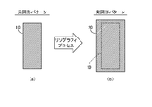
- FIG. 2 is a plan view showing a specific example in which a difference in shape occurs between the original figure pattern 10 and the actual figure pattern 20.
- FIG. 2 In a semiconductor device etc., it is actually necessary to form a very fine and complicated figure pattern on the surface of an actual substrate S such as silicon, but here, for convenience of explanation, a simple as shown in FIG. 2 (a) The case where a basic figure is given as the original figure pattern 10 will be described.
- the original graphic pattern 10 shown in the figure is a pattern consisting of one rectangle, and for example, original graphic data showing formation of a material layer corresponding to the hatched rectangular inner area on the real substrate S. Become.
- a resist layer is formed on the upper surface of the material layer on the actual substrate S, and exposure with light or an electron beam is performed to write on the resist layer.
- the resist layer is developed to remove the non-exposed part, The exposed portion remains as a remaining resist layer (hatched portion).
- the material layer is etched using this remaining resist layer as a mask, theoretically, the internal region (hatched part) of the original figure pattern 10 can be left even for the material layer, On the real substrate S, the same real figure pattern as the original figure pattern 10 shown in FIG. 2A can be obtained.
- the actual figure pattern 20 obtained on the actual substrate S does not exactly match the original figure pattern 10.
- the conditions of the steps of exposure, development and etching included in the lithography process affect the shape of the real figure pattern 20 finally obtained.
- drawing on the resist layer is performed by light or electron beam, but at that time, the exposure area actually drawn on the resist layer by the proximity effect (PE: Proximity Effect) is the original figure It is known that the area is slightly larger than the pattern 10.
- the real figure pattern 20 obtained on the real substrate S is an area which is wider than the original figure pattern 10 (shown by a broken line) as shown in FIG. 2 (b). become.
- the characteristics of the developing solution used in the developing process, the characteristics of the etching solution and plasma used in the etching process, and conditions such as the time of the developing process and the etching process also affect the shape of the actual figure pattern 20. Therefore, when actually manufacturing a semiconductor device or the like, after designing a desired original figure pattern 10 on a computer, the lithography process using this original figure pattern 10 is simulated on a computer, and on the actual substrate S A procedure is performed to estimate the shape of the real graphic pattern 20 that will be formed.
- the figure pattern shape estimation apparatus 100 'shown in FIG. 1 is an apparatus having the function of performing such estimation, and does not actually perform the lithography process (exposure, development, and etching steps) for producing the actual substrate S. In addition, it has a function to estimate the shape of the real figure pattern 20 that will be formed on the real substrate S by simulation.
- the evaluation point setting unit 110 sets an evaluation point E on the original graphic pattern 10. Specifically, figure data including information of an outline indicating the boundary between the inside and the outside of the figure is given to the shape estimation apparatus 100 'as the original figure pattern 10, and the evaluation point setting unit 110 Based on the original graphic pattern 10, processing is performed to set an evaluation point at a predetermined position on the outline.
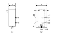
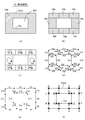
- FIG. 3 is a plan view showing an example in which several evaluation points are set for the original figure pattern 10 shown in FIG. 2A and a process bias (dimension error) generated at each evaluation point.
- FIG. 3A is a plan view showing an example in which evaluation points E11, E12 and E13 are set on the outline of the original figure pattern 10 (rectangular figure) shown in FIG. 2A.
- FIG. 3 shows a simple example in which three evaluation points E11, E12, and E13 are set for convenience of explanation, actually, more evaluation points are set on each side of the rectangle. Ru.
- the present invention proposes a new method for setting this evaluation point, and the specific content thereof will be described in 5 5 and thereafter.
- FIG. 3 (b) is a plan view showing the contour (solid line) of the real figure pattern 20 shown in FIG. 2 (b) in contrast to the contour (broken line) of the original figure pattern 10 shown in FIG. 2 (a).
- a state is shown in which the outline of the real figure pattern 20 shown by a solid line extends outward by the dimension y as compared with the outline of the original figure pattern 10 shown by a broken line. Therefore, the width a of the original figure pattern 10 is expanded to the width b of the actual figure pattern 20.
- the vertical width is also slightly expanded.
- the evaluation points E21, E22 and E23 on the real figure pattern 20 are evaluation points determined as points corresponding to the evaluation points E11, E12 and E13 on the original figure pattern 10.
- the evaluation point E21 is defined as a point obtained by shifting the evaluation point E11 by the predetermined dimension y11 toward the outer side in the normal direction of the outline indicated by the broken line.
- the evaluation point E22 is defined as a point obtained by shifting the evaluation point E12 by the predetermined dimension y12 toward the outside of the normal line direction of the outline shown by the broken line
- the evaluation point E23 is an outline showing the evaluation point E13 by the broken line. It is defined as a point shifted by a predetermined dimension y13 toward the outside in the normal direction of.
- the deviation amount y in the normal direction of the contour line generated for each evaluation point E is I will use it.
- this deviation amount y is called “process bias y” because it is a bias amount generated due to the lithography process.
- the process bias y is a value having a positive or negative sign, and in the embodiment shown below, the direction in which the exposed portion (drawing portion) of the figure is thick is defined as a positive value, and the narrowing direction is defined as a negative value.
- the inside of the figure surrounded by the outline becomes the exposure part (drawing part), and therefore, when shifted in the outward direction of the outline, a positive value is deviated in the inward direction of the outline. Is a negative value.
- the process biases y11, y12 and y13 take positive values.
- evaluation points E11, E12, and E13 are shown in FIG. 3 for the sake of convenience of the description, in actuality, more evaluation points E are defined on the outline of the original figure pattern 10. Ru. Therefore, if the process bias y can be estimated for each evaluation point E, the position of each evaluation point E after the lithography process can be determined by shifting each evaluation point E in the normal direction of the contour by the process bias y. The outline position of the real figure pattern 20 can be estimated.
- the value of process bias y of each evaluation point E is different for each individual evaluation point.
- the values of the process biases y11, y12 and y13 are respectively individual values. This is because the relative positions of the evaluation points E11, E12, and E13 with respect to the original figure pattern 10 are different from each other, and therefore the influence of the lithography process is also different, and a difference also occurs in the amount of deviation generated in each. Therefore, in order to increase the estimation accuracy in estimating the shape of the actual figure pattern 20 by simulation based on the original figure pattern 10, the influence of the lithography process is appropriately predicted for each individual evaluation point, and an appropriate process bias is provided. It is important to find y.
- each evaluation point E is first set on the original graphic pattern 10 by the evaluation point setting unit 110.
- each evaluation point E may be set at a predetermined position on the outline based on the information of the outline indicating the boundary between the inside and the outside of the figure included in the original figure pattern 10.
- evaluation points can be set continuously at predetermined intervals along the outline (the evaluation point setting method specific to the present invention will be described in ⁇ 5 and later).
- the feature amount extraction unit 120 extracts feature amounts indicating features around each evaluation point E for the original figure pattern 10.
- the feature amount x for one evaluation point E is a value indicating the feature around the evaluation point E.
- the feature amount extraction unit 120 includes an original image creation unit 121, an image pyramid creation unit 122, and a feature amount calculation unit 123, as shown in FIG.
- the original image creation unit 121 creates an original image composed of a set of pixels each having a predetermined pixel value based on the given source graphic pattern 10. For example, when the original figure pattern 10 as shown in FIG. 2A is given, the pixel value 1 is for the pixel inside the rectangle (the pixel in the hatched portion in the figure), and the pixel value 0 for the pixel outside the rectangle. To create an original image consisting of a binary image.
- the image pyramid creation unit 122 performs an image pyramid creation process including a reduction process of reducing the original image to create a reduced image, and creates an image pyramid composed of a plurality n of hierarchical images.
- the n hierarchical images constituting each hierarchy of the image pyramid are all images obtained by performing predetermined image processing on the original image generated by the original image generation unit 121, and have different sizes. There is.
- Such a collection of hierarchical images is referred to as an “image pyramid” because, when hierarchical images are formed sequentially by stacking hierarchical images from large to small size, it is as if pyramids are formed. It is to see.
- the feature amount calculation unit 123 calculates a feature amount based on the pixel values of the pixels in the vicinity of the evaluation point E for each of the n hierarchical images forming the hierarchy of the image pyramid. Specifically, the feature amount x1 is calculated based on the pixel values of the pixels in the vicinity of the evaluation point E in the first hierarchical image, and the pixel values of the pixels in the vicinity of the evaluation point E in the second hierarchical image are calculated. The feature amount x2 is calculated based on the above, and similarly, the feature amount xn is calculated based on the pixel values of the pixels in the vicinity of the evaluation point E in the n-th hierarchical image. n feature quantities x1 to xn are extracted.
- n feature amounts x1 (E11) to xn (E11) are extracted for the evaluation point E11, and n feature amounts x1 (E12) for the evaluation point E12. ... To xn (E12) are extracted, and n feature amounts x1 (E13) to xn (E13) are extracted for the evaluation point E13.
- the bias estimation unit 130 is a process that indicates the amount of deviation between the position of the evaluation point E on the original figure pattern 10 and the position on the actual figure pattern 20 based on the feature quantity x extracted by the feature quantity extraction unit 120. A process is performed to estimate the bias y.
- the bias estimation unit 130 includes a feature amount input unit 131 and an estimation operation unit 132.
- the feature amount input unit 131 is a component to which the feature amounts x1 to xn calculated for the evaluation point E by the feature amount calculation unit 123 are input, and the estimation operation unit 132 performs learning obtained in the learning step performed in advance. Based on the information L, estimated values corresponding to the feature quantities x1 to xn are obtained, and the obtained estimated values are output as an estimated value y of the process bias for the evaluation point E.
- the estimation calculation unit 132 estimates the process bias value as the amount of deviation in the normal direction of the outline. It will output y.
- the process bias y11 for the evaluation point E11, the process bias y12 for the evaluation point E12, and the process bias y13 for the evaluation point E13. are respectively output from the estimation operation unit 132 as estimated values.
- the figure pattern shape correction apparatus 100 corrects the shape of the original figure pattern 10 using the figure pattern shape estimation apparatus 100 'described above, and as shown in FIG. 1, the figure pattern shape estimation apparatus 100' A pattern correction unit 140 is further provided in addition to the evaluation point setting unit 110, the feature value extraction unit 120, and the bias estimation unit 130, which are components of the above.
- the pattern correction unit 140 is a component that performs correction on the original figure pattern 10 based on the estimated value y of the process bias output from the bias estimation unit 130, and a corrected figure pattern obtained by the correction by the pattern correction unit 140. 15 is the final output of the shape correction apparatus 100 of this figure pattern.
- the evaluation point E11 is moved to the left (inside the rectangle) by the process bias y11
- the evaluation point E12 is moved to the left (inside the rectangle) by the process bias y12.
- the evaluation point E13 may be moved upward (inside the rectangle) by the process bias y13.
- a greater number of evaluation points are defined, so that correction is made to move all these evaluation points by the size corresponding to the process bias to the inside of the rectangle, and new evaluation points are connected.
- the real figure pattern 25 obtained is It does not exactly match the original graphic pattern 10 of the original design (for example, the width of the rectangle formed on the real substrate S does not exactly become a). This is because the figures included in the original figure pattern 10 and the figures included in the corrected figure pattern 15 have different sizes and shapes, so that differences occur in the effects such as proximity effect when the lithography process is performed.
- the actual figure pattern 25 obtained as a result of performing the lithography process using the corrected figure pattern 15 is Since the pattern becomes closer to the original figure pattern 10, the actual lithography process is performed using the corrected figure pattern 15 obtained by the correction by the pattern correction unit 140 rather than performing the actual lithography process using the original figure pattern 10 as it is. More accurate figure patterns can be obtained on the actual substrate S by executing. That is, if correction is performed by the pattern correction unit 140, it is true that the error is reduced.
- the process of giving the corrected figure pattern 15 output from the pattern correction unit 140 to the figure pattern shape correction apparatus 100 is repeated again. That is, the corrected figure pattern 15 is given to the figure pattern shape estimation apparatus 100 'as a new original figure pattern, and this new original figure pattern (corrected figure pattern 15) is described in ⁇ 1.1. Processing is performed. Specifically, the evaluation point setting unit 110 sets each evaluation point E on the corrected graphic pattern 15, the feature amount extraction unit 120 extracts a feature amount for each evaluation point E, and the bias estimation unit 130 An estimated process bias value y for each evaluation point E is calculated. Then, using the calculated process bias estimated value y, the pattern correction unit 140 performs another correction process.
- the figure pattern shape correction apparatus 100 shown in FIG. 1 has a function of repeatedly executing correction on the figure pattern. That is, a first corrected figure pattern 15 is obtained based on the original figure pattern 10, a second corrected figure pattern is obtained based on the first corrected figure pattern 15, and a second corrected figure pattern is obtained based on the second corrected figure pattern. Thus, the third corrected figure pattern is obtained, and the correction process of ... is repeated. Each time the correction processing is performed, the shape error between the original graphic pattern and the graphic pattern obtained by simulation is reduced.
- the evaluation point setting unit 110, the feature value extraction unit 120, the bias estimation unit 130, and the pattern correction unit 140 shown in FIG. 1 are all configured by incorporating a predetermined program in a computer. Therefore, the figure pattern shape estimation apparatus 100 'and the figure pattern shape correction apparatus 100 according to the invention of the prior application are actually realized by incorporating a dedicated program into a general-purpose computer.
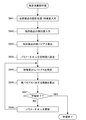
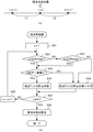
- FIG. 4 is a flow chart showing a product design / production process using the figure pattern shape correction apparatus 100 shown in FIG.
- a product design stage is performed.
- This product design stage is a process of creating a figure pattern for forming a semiconductor device or the like, and the original figure pattern 10 shown in FIG. 1 is created at this product design stage.
- the apparatus itself which designs products, such as a semiconductor device etc., and produces a figure pattern is already a well-known apparatus, detailed description is abbreviate
- the evaluation point setting step of the next step S2 is a step executed in the evaluation point setting unit 110 shown in FIG.
- the feature quantity extraction step of the subsequent step S3 is a stage executed in the feature quantity extraction unit 120 shown in FIG. 1, and as described above, n kinds of feature quantities x1 to xn are extracted for one evaluation point E. (Detailed extraction procedure is described in ⁇ 2).
- the process bias estimation step of step S4 is a step executed in the bias estimation unit 130 shown in FIG. 1, and as described above, the process is performed using n feature quantities x1 to xn for one evaluation point E. A bias estimate y is obtained (a detailed calculation procedure will be described in ⁇ 3).
- the pattern shape correction step of step S5 is a step executed in the pattern correction unit 140 shown in FIG. 1, and as described above, using the process bias estimated value y obtained for each evaluation point E, By correcting the pattern 10, a corrected figure pattern 15 is obtained. Since such correction is not sufficient only once, the process of returning to step S2 is repeated until it is determined that "correction is completed" in step S6. That is, by treating the corrected figure pattern 15 obtained in step S5 as a new original figure pattern 10, the processes of steps S2 to S5 are repeatedly executed.
- step S6 when it is determined that “correction is completed” in step S6, the process proceeds to step S7, and the lithography process is performed.
- the determination of "correction completed” is, for example, that "the difference between the position on the original figure pattern and the position on the figure pattern obtained by simulation for a certain percentage of evaluation points E is less than a predetermined reference value" Specific conditions are met.
- step S7 an actual process of exposure, development, and etching is performed based on the finally obtained corrected figure pattern, and the actual substrate S is manufactured.
- the stages of steps S1 to S6 are processes executed on a computer, and the stage of step S7 is a process executed on the actual substrate S.
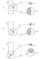
- FIG. 5 is a plan view showing a concept of grasping features around the evaluation points E11, E12 and E13 defined on the outline of the rectangular figure pattern 10.
- FIG. 5A shows a state in which the features of the reference circle C1 and the reference circle C2 are extracted at the evaluation point E11 set at the center of the right side of the rectangle.
- the reference circles C1 and C2 are both circles centered on the evaluation point E11, the reference circle C2 is a larger circle than the reference circle C1.
- FIG. 5 (b) shows the evaluation point E12 set at the lower right side of the rectangle
- FIG. 5 (c) shows two reference circles C1, C2 at the evaluation point E13 set at the center of the lower side of the rectangle. The state which extracted the internal feature of C2 is shown.
- the left half of the evaluation point E11 and the evaluation point E12 is inside the figure (hatched area) and the right half is outside the figure (blank area).
- the internal feature of the reference circle C1 for the evaluation point E13 is that the upper half is inside the figure (hatched area) and the lower half is outside the figure (blank area), and within the reference circle C1 of the evaluation points E11 and E12. It is a 90 ° rotation of the feature of (1), but there is no difference in the occupancy of the hatched area.
- the internal characteristics of the reference circle C2 are compared for each of the evaluation points E11, E12, and E13, it can be seen that the distributions of hatching regions are different from each other and have different characteristics.
- the proximity effect in electron beam exposure includes various effects such as an effect due to forward scattering having a narrow influence range and an effect due to backscattering having a wide influence range.
- forward scattering is described as a phenomenon in which electrons of small mass are spread while being scattered by molecules in the resist when the electron beam is irradiated to the layer to be formed including the resist layer or the like
- backscattering is The phenomenon is described as a phenomenon in which electrons scattered and reflected around the surface of a metal substrate or the like under the resist layer are diffused in the resist layer.
- a process bias is also generated by the etching process, and the size thereof changes according to the loading phenomenon at the time of etching.
- this loading phenomenon also results from the combination of various components such as a component having a narrow influence range and a component having a wide influence range.
- the value of the process bias y for one evaluation point E becomes a value determined by fusing phenomena with various scales. Therefore, extracting various feature amounts from the feature amount for the narrow range to the feature amount for the wide range is different for the various phenomena in each process affecting the process bias, each having a different range of influence. Important for accurate simulation. Therefore, in the prior application invention, for one evaluation point E, feature amounts for various regions around it are extracted from near to far. As described above, in order to extract a plurality of feature amounts for one evaluation point E, the prior invention adopts a method of creating an "image pyramid" composed of a plurality of hierarchical images having different sizes. The image pyramid contains information in which various phenomena having different influence ranges are multiplexed.
- FIG. 6 is a diagram showing an outline of processing executed in the feature quantity extraction unit 120 and the bias estimation unit 130 shown in FIG.
- the original image Q1 shown at the top of the figure is an image created by the original image creation unit 121 shown in FIG. 1 and is an image corresponding to the given source graphic pattern 10.
- the original figure pattern 10 is data created by a design device of a semiconductor device or the like, and becomes data indicating a figure as shown in FIG. 2A, but usually indicates an outline of the figure. It is given as vector data (data indicating the connection between the coordinate value of each vertex and each vertex).
- the original image creation unit 121 executes a process of creating an original image Q1 composed of a set of pixels each having a predetermined pixel value based on the given data of the original graphic pattern 10. For example, if a pixel having a pixel value of 1 is arranged inside the figure constituting the original figure pattern 10 and a pixel having a pixel value of 0 is arranged outside, the original image Q1 consisting of a collection of many pixels U Can be created.
- the original image Q1 shown in FIG. 6 is an image composed of such a set of pixels U, and has rectangular figures included in the original figure pattern 10 as image information, as shown by the broken lines.
- the evaluation point setting unit 110 sets an evaluation point E on the outline of this figure. Although only one evaluation point E is depicted in FIG. 6 for the sake of convenience, in actuality, a large number of evaluation points are set along the outline of the figure.
- the image pyramid creation unit 122 shown in FIG. 1 creates an image pyramid PP based on the original image Q1.
- the image pyramid PP is composed of a plurality of hierarchical images each having a different size.
- the figure shows an image pyramid PP composed of n plural (n (2) hierarchical images P1 to Pn.
- the specific procedure for creating hierarchical images P1 to Pn from the original image Q1 will be described in ⁇ 2.
- the hierarchical images P1 to Pn are created by reduction processing to reduce the number of pixels.
- the hierarchical image P1 is an image of the same size as the original image Q1 (image having the same number of vertical and horizontal pixels), whereas the hierarchical image P2 is a reduced-size image of small size
- the hierarchical image P3 is a smaller size image obtained by further reducing the hierarchical image P2.
- hierarchical images P1 to Pn are created such that the image size gradually decreases based on the original image Q1.
- the state in which a plurality of hierarchical images of different sizes are vertically arranged is in the form of a pyramid as shown in the figure, so in the prior application, an assembly of a plurality of hierarchical images P1 to Pn is referred to as an image pyramid PP. I'm calling. Since all of the hierarchical images P1 to Pn are created based on the original image Q1, the hierarchical images P1 to Pn have information of the original graphic pattern 10, and the position of the evaluation point E can be defined for each of them. In the figure, rectangular figures are drawn on each of the hierarchical images P1 to Pn, and evaluation points E are arranged on the outlines thereof.
- the feature quantity calculation unit 123 illustrated in FIG. 1 performs a process of calculating feature quantities based on the pixel values of the pixels in the vicinity of the evaluation point for each hierarchical image constituting the image pyramid.
- FIG. 6 shows a state in which the feature amounts x1 to xn of the evaluation point E are extracted from the n hierarchical images P1 to Pn constituting the image pyramid PP.
- the illustrated feature quantities x1 to xn are values indicating features around the same evaluation point E, but the feature quantity x1 is a pixel value of a pixel near the evaluation point E on the first hierarchical image P1.
- the feature amount x2 is a value calculated based on the pixel values of pixels in the vicinity of the evaluation point E on the second hierarchical image P2, and the feature amount x3 is a third value. This is a value calculated based on the pixel values of the pixels in the vicinity of the evaluation point E on the hierarchical image P3.
- a specific calculation procedure of each of the feature quantities x1 to xn will be described in ⁇ 2.
- n feature quantities x1 to xn are calculated for each of a large number of evaluation points.
- each of the feature quantities x1 to xn is a predetermined scalar value, n feature quantities x1 to xn are obtained for each evaluation point E, respectively. Therefore, if the n feature quantities x1 to xn are grasped as an n-dimensional vector, the feature quantity extraction unit 120 performs processing for extracting a feature quantity consisting of an n-dimensional vector for one evaluation point E. .
- the feature quantity (n-dimensional vector) for each evaluation point extracted in this manner is input by the feature quantity input unit 131 in the bias estimation unit 130 and is given to the estimation operation unit 132.
- the estimation operation unit 132 is constituted by a neural network, and based on the learning information L obtained by the learning step carried out in advance, the feature quantities x1 to xn given as n-dimensional vectors.
- calculation is performed to calculate the estimated value y (scalar value) of the process bias for the evaluation point E. Specific calculation procedures will be described in ⁇ 3.
- the present invention is not limited to the application to the manufacturing process of the present invention, and can be applied to the manufacturing process of various products including a lithography process.
- the invention of the prior application or the present invention can be used in the manufacturing process of various products including lithography processes such as NIL (Nano Imprint Lithography) and EUV (Extreme UltraViolet Lithography).
- NIL Nano Imprint Lithography
- EUV ExtraViolet Lithography
- correction may be performed on the original figure pattern so that the actual figure pattern on the master template produced from the original figure pattern through exposure lithography matches the original figure pattern.
- correction may be performed on the original figure pattern so that the actual figure pattern on the replica template produced through imprinting from the master template matches the original figure pattern.
- lithography processes such as Micro Electro Mechanical Systems (MEMS), Large-size Photomask (LSPM), lead frames, metal masks, metal mesh sensors, color filters, etc. Applicable to
- the feature quantity extraction unit 120 has an original image creation unit 121, an image pyramid creation unit 122, and a feature quantity calculation unit 123, and the feature quantity extraction process of step S3 in the flowchart of FIG. It has a function to execute.
- This feature quantity extraction process is actually performed according to each procedure shown in FIG.
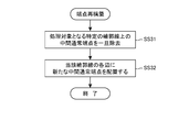
- steps S31 and S32 are procedures executed by the original image creation unit 121
- steps S33 to S36 are procedures executed by the image pyramid creation unit 122
- step S37 is a feature quantity calculation unit 123.
- the original image creation unit 121 has a function of creating an original image composed of a set of pixels each having a predetermined pixel value based on the given source graphic pattern 10, and performs steps S31 and S32 of the flowchart of FIG. Run. First, in step S31, a process of inputting the original graphic pattern 10 is performed, and in the subsequent step S32, an original image creation process is performed.
- ⁇ 1 for convenience of explanation, a simple pattern consisting of only one rectangular figure as shown in FIG. 2A is shown as an example of the original figure pattern 10 input in step S 31.
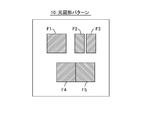
- the original figure pattern 10 including five figures F1 to F5 (rectangles) as shown in FIG. 8 is given.
- the original figure pattern 10 given to the figure pattern shape correction apparatus 100 is usually vector data indicating the outline of the figure. Therefore, although FIG. 8 shows hatching in each figure F1 to F5, actually, in the original figure pattern 10, the coordinate value of each vertex of five rectangles F1 to F5 and each vertex are indicated. It is given as vector data indicating the connection relation of
- the original image creation process of step S32 is a process of creating data (raster data) of the original image Q1 composed of a group of pixels based on the original graphic pattern 10 given as such vector data.
- the original image creation unit 121 defines a mesh consisting of a two-dimensional array of pixels U, superimposes the original figure pattern 10 on this mesh, and configures the position of each pixel U and the original figure pattern 10
- a process of determining the pixel value of each pixel U is performed based on the relationship with the positions of the outlines of the figures F1 to F5.
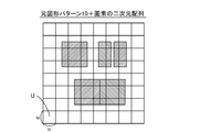
- FIG. 9 is a plan view showing a state in which processing of superposing the original figure pattern 10 on the mesh formed by the two-dimensional array of the pixels U in the original image creation unit 121 is performed.
- a mesh is defined in which pixels U having pixel dimensions u in the vertical and horizontal directions are two-dimensionally arrayed, and a large number of pixels U are arranged at the pitch u in the vertical and horizontal directions.
- the pixel size u is set to an appropriate value that can represent the shapes of the figures F1 to F5 with a sufficient resolution. As the pixel size u is set smaller, the resolution of shape representation is improved, but the processing load on the later becomes heavier.
- pixel values are defined for the individual pixels U based on the relationship with the positions of the outlines of the figures F1 to F5. There are several ways to define pixel values.
- the most basic definition method recognizes the inner area and the outer area of each figure F1 to F5 based on the original figure pattern 10, and sets the occupancy rate of the inner area in each pixel U as the pixel value of the pixel It is a method.
- the hatched area is the inner area of each of the figures F1 to F5
- the white area is the outer area. Therefore, when this method is adopted, the pixel value of each pixel is defined as the occupancy rate (0 to 1) of the internal region (hatched region) in the pixel in the superimposed state as shown in FIG.
- An image in which pixel values are defined in this manner is generally called an "area density map".
- FIG. 10 is a view showing an area density map M1 created on the basis of “original graphic pattern 10 + two-dimensional array of pixels” shown in FIG.
- each cell is each pixel defined in FIG. 9, and the numbers in the cell are pixel values defined for each pixel.
- the blank cell is a pixel having a pixel value 0 (illustration of the pixel value 0 is omitted).
- a pixel having a pixel value of 1.0 is a pixel having 100% occupancy of the hatched area in FIG. 9, and a pixel having a pixel value of 0.5 has a hatched area in FIG.
- the occupancy rate of the pixel is 50%.
- the area density map M1 is a binary image in which the inside of the figure is represented by pixel value 1 and the outside of the figure is represented by pixel value 0. Since a value indicating the ratio is given as a pixel value, the whole is a monochrome gradation image.
- the pixel value of each pixel is defined as the sum of the lengths of the outlines present in the pixel.
- An image in which pixel values are defined in this manner is generally called an "edge length density map".
- a unit of the length of the outline for example, a unit having a pixel size u of 1 may be used.
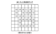
- FIG. 11 is a view showing an edge length density map M2 created on the basis of “original graphic pattern 10 + two-dimensional array of pixels” shown in FIG.
- each cell is each pixel defined in FIG. 9, and the numbers in the cell are defined as the sum of the lengths of the outlines present in each pixel (the length with the pixel size u being 1). Pixel value.
- the blank cell is a pixel having a pixel value 0 (illustration of the pixel value 0 is omitted).
- a pixel having a pixel value of 1.0 is a pixel having a length u of an outline existing in the pixel in FIG.
- this edge length density map M2 is basically a monochrome gradation image showing the density distribution of outlines, it becomes an image having a property considerably different from the area density map M1 described above. However, it is a very useful image in extracting feature quantities for evaluation points E defined on outlines.
- FIG. 12 is a plan view showing an original figure pattern 10 including such dose information. Similar to the original figure pattern 10 shown in FIG. 8, the original figure pattern 10 shown in FIG. 12 includes the information of the outline of each figure F1 to F5, but in addition to that, each figure F1 to For each of F5, it contains information that defines the dose amount.
- a dose of 100% is defined for figures F1 to F3, a dose of 50% is defined for figure F4, and a dose of 10% is defined for figure F5. .
- These dose amounts indicate the intensity of light or electron beam to be irradiated (including the case of controlling the total energy amount by the number of exposures) in the exposure step of the lithography process.
- the light or electron beam is irradiated with an intensity of 100% when exposing the inner area of the figures F1 to F3, but 50% when exposing the inner area of the figure F4, When exposing the inner area, light or electron beam is irradiated at an intensity of 10%.
- the dose amount is controlled for each figure at the time of the exposure process, the size of the actual figure pattern 20 formed on the actual substrate S can be adjusted more finely.
- the pixel value of each pixel in the superimposed state as shown in FIG. 9 is the occupancy rate (0 to 1) of the internal area (hatched area) of the specific figure in the pixel and the specific It is defined as the sum of the product of the dose amount of the figure.
- An image in which pixel values are defined in this manner is generally called a "dose density map". This dose density map is also a monochrome gradation image as a whole.
- FIG. 13 is a view showing a dose density map M3 created based on the original figure pattern 10 with a dose amount shown in FIG.
- each cell is each pixel defined in FIG. 9, and the numbers in the cell are pixel values defined for each pixel.
- the blank cell is a pixel having a pixel value 0 (illustration of the pixel value 0 is omitted).
- FIG. 7 shows an example in which the area density map M1 is the original image Q1 as an example.
- the original image Q1 created in step S32 is used as a first preparation image Q1 in the filter process of step S33.
- the first preparation image Q1 is an original image created first based on the original graphic pattern 10, and is a reference image used first in the image pyramid creating process described later.
- the image pyramid creation unit 122 has a function of performing reduction processing to reduce the number of pixels based on the original image Q1 (for example, the area density map M1 shown in FIG. 10) created in step S32 of FIG.
- An image pyramid creation process is performed to create an image pyramid composed of a plurality of hierarchical images having different sizes. In the case of the embodiment described herein, this image pyramid creation process is performed by the procedure shown in steps S33 to S36 of the flowchart of FIG.
- the original graphic pattern 10 as shown in FIG. 8 is input, and in the step S32, a specific image is taken as an example where the area density map M1 shown in FIG. 10 is created as the original image Q1.
- the procedure of the pyramid creation process will be described.
- an image processing filter is applied to the k-th preparation image Qk to perform filter processing for creating the k-th hierarchical image Pk.
- this filtering process is performed as, for example, a convolution operation using a Gaussian filter as an image processing filter.
- FIG. 14 is a plan view showing a procedure for creating the k-th hierarchical image Pk by applying a filtering process using a Gaussian filter GF33 to the preparation image Qk.
- the k-th preparation image Qk shown in FIG. 14 is actually the same as the area density map M1 shown in FIG.
- the area density map M1 shown in FIG. 10 is shown as an 8 ⁇ 8 pixel array for convenience, and the description of the pixel value 0 is omitted, whereas the preparation image Qk shown in FIG. Although shown as an array of 10 pixels and the pixel value 0 is also described, both are substantially the same image.
- FIG. 14 in order to execute the filter processing, pixels having a pixel value 0 are arranged around the area density map M1 consisting of the 8 ⁇ 8 pixel array shown in FIG. It is only At this stage, the parameter k has an initial value of 1, and the preparation image Qk shown in FIG. 14 is the first preparation image Q1.
- the first preparation image Q1 is nothing but the original image created in the original image creation process in step S32.
- FIG. 14 a convolution operation using a Gaussian filter GF33 is performed.
- the Gaussian filter GF33 is a 3 ⁇ 3 pixel array as shown in the drawing, and the k-th is performed by superposing the Gaussian filter GF33 on a predetermined position of the k-th preparation image Qk and performing product-sum operation processing Hierarchical images Pk (filtered images) are obtained.
- FIG. 15 is a plan view showing the k-th hierarchical image Pk obtained by the filter processing shown in FIG.
- the k-th hierarchical image Pk has a 10 ⁇ 10 pixel array similarly to the k-th preparatory image Qk, and the pixel values of the individual pixels are obtained by product-sum operation using the Gaussian filter GF33. It becomes a value.
- a pixel value of 0.375 is given to the target pixel .
- the pixel value is obtained by superposing the illustrated Gaussian filter GF33 on the 3 ⁇ 3 pixel array (9 pixels centered on the fourth row and third column pixels) surrounded by a bold frame in FIG.
- the product of the pixel values of the pixels overlapped at the same position is determined as the sum of the nine products.
- the pixel value 0.375 of the pixel of interest is “(1/16 ⁇ 0) + (2/16 ⁇ 0.25) + (1/16 ⁇ 0.5) + (2/16 ⁇ 0) ) + (4/16 x 0.5) + (2/16 x 1.0) + (1/16 x 0) + (2/16 x 0.25) + (1/16 x 0.5) "
- the product-sum operation value is obtained as Such filter processing by product-sum operation is a process generally known as a convolution operation process on an image, and thus the detailed description is omitted here.
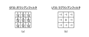
- the convolution operation is performed using a Gaussian filter GF33 consisting of a 3 ⁇ 3 pixel array as shown in FIG. 16A as an image processing filter.
- the convolution operation may be performed using a Laplacian filter LF33 having a 3 ⁇ 3 pixel arrangement as shown in b).
- filtering using a Gaussian filter has an effect of blurring the outline of an image
- filtering using a Laplacian filter has an effect of enhancing the outline of an image.
- the k-th layered image Pk having slightly different features can be obtained with respect to the k-th preparation image Qk, and therefore, a plurality of layered images having different features are provided. It is effective in creating an image pyramid.
- the image processing filter used for the filter processing in step S33 is not limited to the Gaussian filter GF33 shown in FIG. 16 (a) or the Laplacian filter LF33 shown in FIG. 16 (b). It is possible to use processing filters. Also, the size of the image processing filter to be used is not limited to the 3 ⁇ 3 pixel array, and it is possible to use an image processing filter of any size. For example, a Gaussian filter GF55 consisting of a 5 ⁇ 5 pixel array as shown in FIG. 17 (a) or a Laplacian filter LF55 consisting of a 5 ⁇ 5 pixel array as shown in FIG. 17 (b) may be used. .
- step S34 it is determined in step S34 whether or not the parameter k has reached a predetermined set value n. If k ⁇ n, reduction of step S35 is performed. Processing is performed.
- This reduction process is a process of creating an image having a smaller number of pixels than the target image based on a predetermined target image.
- the (k + 1) -th preparation image Q (k + 1) is created by executing the reduction process on the k-th hierarchical image Pk created in the filter process of step S33. Processing is performed. Therefore, the preparation image Q (k + 1) is an image smaller in size than the hierarchical image Pk (an image in which the number of vertical and horizontal pixels in the pixel array is small).
- FIG. 18 is a plan view showing a procedure for creating the (k + 1) th preparation image Q (k + 1) as a reduced image by performing average pooling processing on the k-th hierarchical image Pk. .
- the average pooling process (reduction process) is applied to the hierarchical image Pk consisting of the 4 ⁇ 4 pixel array shown in FIG. 18A to obtain 2 ⁇ 2 image shown in FIG.
- a preparation image Q (k + 1) composed of a pixel array is created as a reduced image.
- the average pooling process shown in FIG. 18 is a process of converting (reducing) four pixels consisting of a 2 ⁇ 2 pixel array into one pixel, and calculates the average value of the pixel values of the original four pixels, By using the pixel value of one pixel after conversion, a reduced image is created.
- four pixels pixels within a bold frame
- the preparation image Q (FIG. 18B).
- conversion (reduction) is performed to one pixel indicated by a thick frame.
- the pixel value 0.5 of the thick frame pixel after this conversion (reduction) is the average value of the pixel values of the original four pixels.
- FIG. 19 is a plan view showing a procedure for creating the (k + 1) th preparation image Q (k + 1) as a reduced image by performing max pooling processing on the k-th hierarchical image Pk It is. Specifically, by performing max pooling processing (reduction processing) on the hierarchical image Pk consisting of the 4 ⁇ 4 pixel array shown in FIG. 19A, the 2 ⁇ 2 image shown in FIG. 19B is obtained. A preparation image Q (k + 1) composed of a pixel array is created as a reduced image.
- the max pooling process shown in FIG. 19 is a process to convert (reduce) four pixels consisting of a 2 ⁇ 2 pixel array into one pixel, similarly to the average pooling process shown in FIG. A reduced image is created by setting the maximum value of the pixel values of the four pixels in the above as the pixel value of one pixel after conversion. For example, four pixels (pixels within a bold frame) consisting of a 2 ⁇ 2 pixel array arranged at the upper left of the hierarchical image Pk shown in FIG. 19A are the preparation image Q (FIG. 19B). On k + 1), conversion (reduction) is performed to one pixel indicated by a thick frame. The pixel value 1.0 of the thick frame pixel after this conversion (reduction) is the maximum value of the pixel values of the original four pixels.
- each pooling process shown in FIGS. 18 and 19 is a reduction process for converting four pixels consisting of a 2 ⁇ 2 pixel array into a single pixel, it is of course made up of a 3 ⁇ 3 pixel array It is also possible to perform a reduction process to convert nine pixels into a single pixel, or to perform a reduction process to convert six pixels of a 3 ⁇ 2 pixel array to a single pixel. It is.
- the image pyramid creating unit 122 replaces the plurality of m adjacent pixels with a single pixel whose pixel value is the average value of the pixel values of the plurality of m adjacent pixels. It is possible to create a reduced image by performing pooling processing, or to replace a plurality of m adjacent pixels with a single pixel whose pixel value is the maximum value of the pixel values of the plurality m of adjacent pixels. A reduced image can also be created by performing pooling processing. Of course, other reduction processes can also be performed as the reduction process of step S35.
- step S35 by performing conversion to reduce the number of pixels with respect to the hierarchical image Pk, a process capable of creating a small-sized preparatory image Q (k + 1), in other words, “the number of pixels has decreased Any reduction process may be performed in step S35 as long as it is a process of creating a “reduced image”.
- step S35 when the reduction process of step S35 is completed, the parameter k is increased by 1 in step S36, and the filter process of step S33 is performed again.
- n an appropriate value may be set in advance as the number of layers of the image pyramid (that is, the total number of layer images constituting the image pyramid).
- the value of n is set larger, the number n of feature quantities extracted for one evaluation point E increases, so that more accurate simulation is possible, but the computational load increases.
- the reduction process of step S35 is repeated, the size of the image decreases more and more, so if the value of n is set too large, the reduction process of step S35 can not be performed. Therefore, in practice, the value of n may be set appropriately in consideration of the size of the original image Q1 and the computational burden.
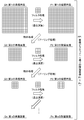
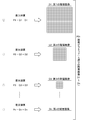
- FIG. 20 is a plan view showing the procedure (procedure of steps S33 to S36 in FIG. 7) of creating the image pyramid PP composed of n kinds of hierarchical images P1 to Pn in the image pyramid creating unit 122.
- step S33 filter processing is performed on the first preparation image Q1.
- a first hierarchical image P1 as shown in the upper right of FIG. 20 is created by a convolution operation using a Gaussian filter GF33 consisting of a 3 ⁇ 3 pixel array.
- the size of the first hierarchical image P1 is the same as the size of the first preparation image Q1.
- step S35 the reduction process (for example, average pooling process) is performed on the first hierarchical image P1, and a second preparation image Q2 shown in the middle left of FIG. 20 is created.
- the size of the second preparation image Q2 is smaller than the size of the first hierarchical image P1.
- step S36 the value of the parameter k is updated to 2, and the filtering process of step S33 is performed again. That is, the second hierarchical image P2 as shown in the middle right of FIG. 20 is created by the convolution operation using the Gaussian filter GF33 consisting of a 3 ⁇ 3 pixel array.
- the size of the second hierarchical image P2 is the same as the size of the second preparation image Q2.
- step S35 the reduction process of step S35 is executed again. That is, reduction processing (for example, average pooling processing) is performed on the second hierarchical image P2, and a third preparation image Q3 shown in the lower left of FIG. 20 is created.
- the size of the third preparation image Q3 is smaller than the size of the second hierarchical image P2.
- step S36 the value of the parameter k is updated to 3, and the filtering process of step S33 is performed again. That is, the third hierarchical image P3 as shown in the lower right of FIG. 20 is created by the convolution operation using the Gaussian filter GF33 consisting of a 3 ⁇ 3 pixel array.
- the size of the third hierarchical image P3 is the same as the size of the third preparation image Q3.
- the image pyramid PP is configured by n hierarchical images different in size from the first hierarchical image P1 to the n-th hierarchical image Pn.
- the image pyramid creation unit 122 has a function of performing filter processing using a predetermined image processing filter on the original image Q1 or the reduced image Q (k + 1).
- an image pyramid PP composed of a plurality of hierarchical images P1 to Pn is created.
- the image pyramid creation unit 122 sets the original image created by the original image creation unit 121 as the first preparation image Q1, and filters the kth preparation image Qk (where k is a natural number).
- the resulting image be the k-th hierarchical image P k
- the image obtained by the reduction process on the k-th hierarchical image P k be the (k + 1) th preparatory image Q (k + 1)
- an image pyramid PP made up of a plurality n of layer images including the first layer image P1 to the n-th layer image Pn is created.
- the reduction process of step S35 is an essential process in the procedure shown in the flowchart of FIG.
- the filtering process of step S33 is not necessarily a necessary process.
- the pixel value of each pixel can be influenced by the pixel value of the surrounding pixel.
- by adding the filter processing it is possible to create a plurality of hierarchical images rich in variations, and it becomes possible to extract feature quantities containing more diverse information, and as a result, it is more accurate. Simulation is possible. Therefore, practically, it is preferable to alternately execute the reduction process and the filtering process as shown in the flowchart of FIG. 7.
- Step S37 of FIG. 7 the feature amount calculation unit 123 performs processing for calculating feature amounts x1 to xn for each evaluation point E based on the hierarchical images P1 to Pn constituting the image pyramid PP.
- the procedure of calculation processing of the feature amounts x1 to xn will be specifically described.
- FIG. 21 is a plan view showing the procedure for calculating the feature amounts x1 to xn for a specific evaluation point E from the layer images P1 to Pn in the feature amount calculation unit 123.
- the original graphic pattern 10 is formed in each pixel array of the first hierarchical image P1, the second hierarchical image P2, and the third hierarchical image P3.
- a state in which the rectangles (indicated by thick frames) forming the frame are overlapped is shown, and on the right side of FIGS.
- the principle of calculating feature quantities x1, x2, x3 for E is shown.
- Each hierarchy image P1, P2, P3 shown in FIG. 21 is a part of the image which comprises each hierarchy of image pyramid PP.
- n hierarchical images from P1 to Pn are prepared, and n sets of feature amounts x1 to xn are extracted.
- FIG. It is shown that three sets of feature quantities x1, x2, x3 are extracted from P2, P3.
- the first hierarchical image P1 is an image obtained by applying the filtering process to the original image Q1 (first preparation image), and in the illustrated example, has a 16 ⁇ 16 pixel array.
- the second hierarchical image P2 is an image obtained by performing the reduction process and the filter process on the first hierarchical image P1, and in the illustrated example, the 8 ⁇ 8 pixel array is Have.
- the third hierarchical image P3 is an image obtained by performing the reduction process and the filter process on the second hierarchical image P2, and in the illustrated example, has a 4 ⁇ 4 pixel array. There is.
- the hierarchical images P1, P2 and P3 are drawn so that their outlines become squares of the same size, and thus they are all images of the same size.
- the size is gradually reduced to ⁇ 16, 8 ⁇ 8, 4 ⁇ 4, and the size of the image is gradually reduced.
- the outer frames of the hierarchical images P1, P2, and P3 are drawn as squares having the same size, the size of the pixels is gradually increased. In other words, the resolution of the image decreases in the order of the hierarchical images P1, P2, and P3 and gradually becomes coarse.
- each hierarchical image P1, P2, P3 is a raster image consisting of a group of pixels, so a rectangular outline drawn in bold in the figure is actually included as information of the outline itself. It does not mean that it is included as information of the pixel value of each pixel.
- the positions of the rectangles on the hierarchical images P1, P2, and P3 are indicated by thick lines.
- a process of extracting the feature amounts x1 to xn will be described for a specific evaluation point E defined on the outline of the rectangle.
- the rectangles shown by thick frames are arranged at the same relative position with respect to each hierarchical image P1, P2, and P3, and the specific evaluation point E is also the same relative. It is placed in position.
- the feature amount for one evaluation point E is calculated based on the pixel values of the pixels in the vicinity thereof.
- the feature amount x1 for the evaluation point E is extracted based on the first hierarchical image P1.
- the feature quantity calculation unit 123 determines that four pixels located in the vicinity of the evaluation point E from the pixels forming the first hierarchical image P1 (see FIG. Is extracted as a pixel of interest, and the feature amount x1 is calculated by calculation using the pixel values of these four pixels of interest.
- attention is focused on four pixels (pixels hatched in the figure) located in the vicinity of the evaluation point E from the pixels constituting the second hierarchical image P2.
- a feature amount x2 is calculated by extraction as a pixel and calculation using pixel values of these four target pixels.
- a feature amount x2 is calculated by extraction as a pixel and calculation using pixel values of these four target pixels.
- the pixels forming the third hierarchical image P3 four pixels (pixels hatched in the figure) located in the vicinity of the evaluation point E are noted pixels Are extracted, and the feature amount x3 is calculated by calculation using the pixel values of these four target pixels.
- n sets of feature amounts x1 to xn can be extracted for a specific evaluation point E.
- These n sets of feature quantities x1 to xn are parameters indicating features around the same evaluation point E on the original figure pattern 10, but the ranges affected by the original figure pattern 10 are different from each other .
- the feature quantity x1 extracted from the first hierarchical image P1 has a value indicating the feature in the narrow area hatched in the right side of FIG. 21A, but the second hierarchical image P2
- the feature amount x2 extracted from the image becomes a value indicating the feature in a wider area hatched in the right side of FIG. 21B
- the feature amount x3 extracted from the third hierarchical image P3 is The figure on the right side of FIG. 21 (c) is a value indicating the feature in a wider area hatched.
- the value of the process bias y for one evaluation point E is a value determined by fusing phenomena having various scale feelings such as forward scattering and back scattering. Therefore, if various feature quantities x1 to xn are extracted as feature quantities for the same evaluation point E from feature quantities x1 for a very narrow range around it to feature quantities xn for a wider range, the influence range Can perform accurate simulations considering various phenomena that differ from one another.
- FIG. 21 shows a process of extracting n sets of feature amounts x1 to xn for one evaluation point E, but in practice each of a large number of evaluation points defined on the original figure pattern 10 is shown. , N sets of feature quantities x1 to xn are extracted by the same procedure.
- a simple method of using the simple average of the pixel values of the target pixel as the feature amount x can be adopted. For example, as shown in FIG. 21A, in order to extract the feature amount x1 for the evaluation point E from the first layer image P1, the pixel of interest (shown in the vicinity of the evaluation point E) is hatched in the figure. The simple average of pixel values of certain four pixels) may be set as the feature amount x1.
- FIG. 22 is a diagram showing a specific calculation method (a calculation method using a weighted average value as a feature quantity) used in the feature quantity calculation procedure shown in FIG.
- a specific calculation method a calculation method using a weighted average value as a feature quantity
- FIG. 22 an example is shown in which four pixels A, B, C, and D are selected as target pixels located in the vicinity of a specific evaluation point E.
- the target pixels A, B, C, and D can be determined by performing processing of selecting a total of four pixels in order of closeness to the evaluation point E. Therefore, with respect to the pixel values of the four pixels of interest A, B, C, and D, an operation may be performed in which a weighted average taking into consideration the weight according to the distance between the evaluation point E and each pixel is used as the feature amount x.
- x marks are displayed at the center points of the noted pixels A, B, C, D, and broken lines connecting these x marks are drawn.
- the pixel size of each of the target pixels A, B, C, and D is u in both the vertical and horizontal directions, and the broken line is a dividing line dividing the pixel having the pixel size u into halves.
- the distance between the evaluation point E and the central point of each of the target pixels A, B, C, D as the distance between the evaluation point E and each of the target pixels A, B, C, D
- the vertical distance is adopted. Specifically, in the case of the example shown in FIG.
- the horizontal distance a and the vertical distance c are for the pixel of interest A, and the horizontal distance b and the vertical distance c for the pixel of interest B.
- the horizontal distance a and the vertical distance d are obtained, and for the pixel of interest D, the horizontal distance b and the vertical distance d.
- the method of calculating the feature quantity x from the pixel values of the four pixels of interest A, B, C, and D is not limited to the method illustrated in FIG. If the feature amount x reflecting the pixel value can be calculated, it is possible to adopt various other calculation methods.
- four pixels located in the vicinity of the evaluation point E are selected as the target pixels, but the number of target pixels used to calculate the feature amount x is It is not limited to four.
- nine pixels forming a 3 ⁇ 3 pixel array located in the vicinity of evaluation point E are selected as the target pixels, and the pixel values of these nine target pixels are determined according to the distance from evaluation point E. It is also possible to obtain a weighted average in which the weight is taken into consideration and use this as the feature amount x for the evaluation point E.
- the feature quantity calculation unit 123 calculates the feature quantity x for a specific evaluation point E on a specific hierarchical image P
- the specific evaluation is performed from the pixels constituting the specific hierarchical image P.
- a total of j pixels are extracted as the pixel of interest in order of proximity to the point E, and for the pixel values of the extracted j pixels of interest, weighting in consideration of the weight according to the distance
- An arithmetic operation for obtaining an average can be performed, and the value of the obtained weighted average can be used as the feature amount x.
- the modification described here is based on the processing of steps S33 to S36 shown in the flow chart of FIG. 7 and further, when the filtering processing of step S33 is completed, the k th The differential image “Pk ⁇ Qk” for subtracting the kth preparation image Qk from the filtered image Pk (the image referred to as the kth hierarchical image Pk in 2.22.2) is performed to obtain the kth difference image Dk.
- the required processing is added.
- the processing of steps S33 to S36 shown in the flowchart of FIG. 7 is executed as it is, but further, the kth filtered image Pk to the kth preparation image Qk
- the difference operation "Pk-Qk" which subtracts will be performed extra.
- the difference operation “Pk ⁇ Qk” defines, for the k-th filtered image Pk and the k-th preparation image Qk, pixels arranged at the same position on the pixel array as corresponding pixels, on the image Pk
- the difference is obtained by subtracting the pixel value of the corresponding pixel on the image Qk from the pixel value of each pixel, and obtaining a difference image Dk consisting of a new set of pixels whose pixel value is the obtained difference.
- FIG. 23 is a plan view showing a procedure for creating an image pyramid PD composed of n kinds of difference images D1 to Dn by such difference operation "Pk-Qk".
- the first hierarchical image D1 shown in the upper right of the upper row is a difference image obtained by the difference operation “P1-Q1”.
- the second hierarchical image D2 shown in the middle right of FIG. 23 is a difference image obtained by the difference operation “P2-Q2”, and more specifically, the second filtering shown in the middle right of FIG.
- the difference is calculated by subtracting the second preparation image Q2 shown in the middle left from the image P2 (referred to as the second hierarchical image P2 in FIG. 20).
- the third hierarchical image D3 shown on the lower right of FIG. 23 is a difference image obtained by the difference operation “P3-Q3”.
- the third filtered image shown on the lower right of FIG. It is calculated by a difference operation of subtracting the third preparation image Q3 shown on the lower left side from P3 (which is called the third hierarchical image P3 in FIG. 20).
- the difference image obtained by the difference calculation “Pn ⁇ Qn” is the n-th hierarchical image Dn.
- the image pyramid PP is formed of the first hierarchical image (first filtered image) P1 to the nth hierarchical image (nth filtered image) Pn.
- the image pyramid is formed by the first hierarchical image (first differential image) D1 to the nth hierarchical image (nth differential image) Dn. PD will be configured.
- the image pyramid creating unit 122 sets the original image created by the original image creating unit 121 as the first preparation image Q1, and is obtained by filtering the k-th preparation image Qk (where k is a natural number).
- a difference image Dk between the filtered image Pk to be reproduced and the k-th preparation image Qk is obtained, the difference image Dk is taken as a k-th hierarchical image Dk, and an image obtained by reduction processing on the k-th filtered image Pk is
- the first hierarchical image D1 to the n-th hierarchical image Dn are included by alternately executing the filtering process and the reduction process until the n-th hierarchical image Dn is obtained as the preparation image Q (k + 1) of k + 1).
- An image pyramid PD consisting of a plurality n of hierarchical images may be created.
- the k-th hierarchical image Dk constituting the k-th hierarchical layer of the image pyramid PD is the image after the filter processing (filtered image Pk) and the image before the filter processing (preparation image Qk) It means a difference image, and the pixel value of each pixel corresponds to the difference between the pixel values before and after the filter processing. That is, while the k-th hierarchical image Pk in the embodiment described in 2.2 2.2 shows the image after filter processing itself, the k-th hierarchical image Dk in the modification described here is a filter. It will show the difference caused by the treatment.
- the image pyramid PP created in the embodiment described in 2.2 2.2 and the image pyramid PD created in the modification described here are significantly different in the meaning of the hierarchical image as the component thereof. As it turns out, there is no difference in that they are images that show some characteristics of the evaluation point E. Therefore, feature quantities can be extracted from each of the hierarchy images D1 to Dn created in the modification described above, and the feature quantity calculation unit 123 in the present modification includes each hierarchy image D1 to Dn. A process of extracting the feature amounts x1 to xn is performed.
- FIG. 16 and FIG. 17 there are various types of image filters used for filter processing as shown in FIG. 16 and FIG. 17, and various types of reduction processing (pooling processing) are also shown in FIG. 18 and FIG. 19. is there.
- the departure point is the same original image (the first preparation image Q1)
- the contents of each hierarchical image constituting the image pyramid obtained differ depending on the algorithm adopted.
- it is not necessary to use only one image pyramid and a plurality of image pyramids are created by a plurality of algorithms, and feature quantities are respectively extracted from the individual image pyramids. Is also possible.
- the image pyramid creating unit 122 is provided with a function of performing image pyramid creating processing based on a plurality of different algorithms for one original image (first preparation image Q1), and a plurality of image pyramids are created. It may be done.
- the feature quantity calculation unit 123 determines, based on the pixel values of pixels (pixels located around the evaluation point) corresponding to the position of the evaluation point, for each hierarchical image constituting each of the plurality of image pyramids. A process of calculating the feature amount may be performed.
- the image pyramid creating unit 122 performs the image pyramid creating process
- the algorithm of the embodiment described in 2.2 2.2 is adopted as the main algorithm, as shown in FIG.
- a main image pyramid PP composed of P1 to Pn (filtered image) can be created, and as a sub-algorithm, an algorithm of a modification using the differential image Dk described in ⁇ 2.4 (1) as a hierarchical image
- the main image pyramid PP created by the filtering process using a Gaussian filter as illustrated in FIG. 14 can be called a Gaussian pyramid.
- the sub-image pyramid PD configured using the difference image can be called a Laplacian pyramid. Since Gaussian pyramid and Laplacian pyramid become image pyramids whose characteristics are greatly different from each other, they are adopted as main image pyramid PP and sub image pyramid PD, and feature quantities are extracted using two image pyramids. If so, it becomes possible to extract more diverse feature quantities.
- the feature amount calculator 123 sets pixel values of pixels in the vicinity of the evaluation point E for the main layer images P1 to Pn constituting the main image pyramid PP and the sublayer images D1 to Dn constituting the sub image pyramid PD. If processing for calculating the feature amount is performed based on the feature amounts xp1 to xpn calculated from the main layer images P1 to Pn and feature amounts xd1 to xdn calculated from the sub layer images D1 to Dn can be obtained. . That is, a total of 2n feature quantities are extracted for one evaluation point E. In this case, since the feature amount for one evaluation point E is given as a 2n-dimensional vector to the estimation operation unit 132, more accurate estimation operation can be performed.
- the image pyramid creating unit 122 sets the original image created by the original image creating unit 121 as the first preparation image Q1, and the kth preparation image Qk (where k is Let an image obtained by the filtering process for the natural numbers be the k-th main layer image Pk, and an image obtained by the reduction process for the k-th main layer image Pk be the (k + 1) th prepared image Q (k + 1).
- a main image pyramid composed of n plural layer images including the first main layer image P1 to the n-th main layer image Pn Is further calculated, and the difference image Dk between the k-th main hierarchy image Pk and the k-th preparation image Qk is determined, and the difference image Dk is set as the k-th sub-layer image Dk. It is sufficient to create a sub image pyramid consisting of hierarchy images of a plurality n as including a sub-hierarchy image Dn image D1 ⁇ No. n.
- the feature amount calculation unit 123 may calculate the feature amount based on the pixel values of the pixels in the vicinity of the evaluation point E for each hierarchy image constituting the main image pyramid PP and the sub image pyramid PD. . Then, it becomes possible to extract a 2n-dimensional vector as a feature amount for one evaluation point E, and it is possible to perform more accurate estimation operation.
- the original image creation unit 121 creates an original image based on the given original graphic pattern 10.
- the area density map M1 (FIG. 10)
- the edge length density map M2 (FIG. 11)
- the dose density map M3 (FIG. 13)
- Various forms of images can be employed.
- the original image creation unit 121 can adopt various creation algorithms, and the contents differ depending on which algorithm is adopted.
- Various original images can be created.
- the area density map M1 shown in FIG. 10 the edge length density map M2 shown in FIG. 11, and the dose density map M3 shown in FIG. 13 are images created based on the same original figure pattern 10, The pixel values of the individual pixels are different from one another, resulting in different images.
- a plurality of density maps (in other words, a plurality of maps with different resolutions) different in pixel size (size of one pixel) and map size (number of pixels arranged in vertical and horizontal directions)
- a plurality of image pyramids may be created with each of the plurality of density maps as an original image.
- a density map density map with high resolution
- a plurality of density maps having different pixel sizes and map sizes are used as the original image.
- the original image creating unit 121 has a function of creating original images based on a plurality of different algorithms to create a plurality of original images, and the image pyramid creating unit 122 generates the plurality of original images. If it has a function of processing to create separate and independent image pyramids based on the images, multiple image pyramids can be created. Then, if the feature amount calculation unit 123 has a function of calculating the feature amount based on the pixel values of the pixels in the vicinity of the evaluation point E for each hierarchical image constituting each of the plurality of image pyramids, It becomes possible to extract feature quantities composed of higher dimensional vectors, and it is possible to carry out more accurate estimation operations.
- the original image generation unit 121 generates a first original image including the area density map M1 illustrated in FIG. 10, a second original image including the edge length density map M2 illustrated in FIG. 11, and a dose density illustrated in FIG.
- the image pyramid creating unit 122 creates three sets of independent image pyramids based on the three original images. Can. Both image pyramids are image pyramids created based on the same original graphic pattern 10.
- the feature amount calculation unit 123 can perform processing of calculating the feature amount based on the pixel values of the pixels in the vicinity of the evaluation point E for each hierarchical image constituting each of the three image pyramids.
- n feature quantities x1 to xn are extracted from one image pyramid, a total of 3n feature quantities can be extracted for the same evaluation point E. That is, since a 3n-dimensional vector can be given as a feature amount for one evaluation point E, it is possible to perform more accurate estimation operation.
- the bias estimation unit 130 has a feature quantity input unit 131 and an estimation operation unit 132, and has a function of executing the process bias estimation process of step S4 in the flowchart of FIG. .
- a feature quantity (n-dimensional vector) of x1 to xn is input to the feature quantity input unit 131 for one evaluation point E, and the estimation operation is performed by the estimation operation unit 132.
- An estimate y of the process bias for E is obtained.
- a neural network is used as the estimation operation unit 132. Therefore, the detailed configuration and operation of this neural network will be described below.
- neural networks have attracted attention as a technology that forms the basis of artificial intelligence, and are used in various fields including image processing.
- the neural network is a computer construct that simulates the structure of the brain of an organism, and is composed of neurons and edges connecting them.
- FIG. 24 is a block diagram showing an embodiment in which a neural network is used as the estimation operation unit 132 shown in FIG.
- a neural network in the neural network, an input layer, an intermediate layer (hidden layer), and an output layer are defined, and predetermined information processing is performed on the information provided to the input layer in the intermediate layer (hidden layer), The result is output to the output layer.
- the feature quantities x1 to xn for one evaluation point E are given to the input layer as an n-dimensional vector, and the output layer estimates the process bias for the evaluation point E The value y is output.
- the estimated value y of the process bias is an estimated value indicating the amount of deviation in the normal direction of the outline for the evaluation point E located on the outline of the predetermined figure. .
- the estimation operation unit 132 has a neural network having the feature amounts x1 to xn input by the feature amount input unit 131 as input layers and the estimated value y of process bias as an output layer.
- the middle layer of this neural network is composed of a first hidden layer, a second hidden layer,..., An Nth hidden layer which is the Nth hidden layer. These hidden layers have a large number of neurons (nodes), and edges connecting these neurons are defined.
- the feature quantities x1 to xn given to the input layer are transmitted as signals to each neuron through the edge. Finally, a signal corresponding to the estimated value y of the process bias is output from the output layer. Signals in the neural network are transmitted from the neurons of one hidden layer to the neurons of the next hidden layer through operations via edges. The calculation through the edge is performed using learning information L (specifically, parameters W and b described later) obtained at the learning stage.
- FIG. 25 is a diagram showing a specific operation process performed by the neural network shown in FIG.
- the portions shown by thick lines in the figure indicate the first hidden layer, the second hidden layer,..., The Nth hidden layer, and individual circles in each hidden layer connect neurons (nodes) and circles.
- the lines indicate the edges.
- the feature quantities x1 to xn for one evaluation point E are given as n-dimensional vectors to the input layer, and the estimated value y of the process bias for the evaluation point E is a scalar for the output layer. It is output as a value (a dimensional value indicating the amount of deviation in the normal direction of the contour line).
- the first hidden layer is an M (1) -dimensional layer, and is constituted by a total of M (1) neurons h (1,1) to h (1, M (1)), and
- the two hidden layers are M (2) -dimensional layers, and are composed of a total of M (2) neurons h (2, 1) to h (2, M (2)), and the Nth hidden layer is M (N) Layer), and is constituted by a total of M (N) neurons h (N, 1) to h (N, M (N)).
- the arithmetic values of the signals transmitted to the neurons h (1, 1) to h (1, M (1)) of the first hidden layer are respectively calculated using the same code as the arithmetic values h (1, 1)
- the values of these operation values h (1, 1) to h (1, M (1)) are given by the matrix equation shown in the upper part of FIG. Be
- the sigmoid function shown in FIG. 27 (a) the normalized linear function ReLU shown in FIG. 27 (b), the normalized linear function Leakey ReLU shown in FIG. 27 (c), etc.
- the activation function of can be used.
- ⁇ described as an argument of the function f ( ⁇ ) is a matrix [W] and a matrix [x1 to xn] (a feature amount given as an n-dimensional vector to the input layer) as shown in the middle part of FIG. It becomes the value which added matrix [b] to the product with).
- the contents of the matrix [W] and the matrix [b] are as shown in the lower part of FIG. 26, and each component of the matrix (weighting parameter W (u, v) and biasing parameter b (u, v)) Is the learning information L obtained by the learning step described later.
- FIG. 28 is a diagram showing an arithmetic expression for obtaining each value of the second to Nth hidden layers in the diagram shown in FIG. Specifically, the same sign is used for the operation value of the signal transmitted to the neurons h (i + 1, 1) to h (i + 1, M (i + 1)) of the (i + 1) hidden layer (1 ⁇ i ⁇ N) If the arithmetic values h (i + 1, 1) to h (i + 1, M (i + 1)) are represented respectively, the values of these arithmetic values h (i + 1, 1) to h (i + 1, M (i + 1)) are It is given by the matrix equation shown in the upper part of FIG. As the function f ( ⁇ ) on the right side of this equation, as described above, each function shown in FIG. 27 can be used.
- ⁇ described as an argument of the function f ( ⁇ ) is the matrix [W] and the matrices [h (i, 1) to h (i, M (i))] as shown in the middle part of FIG. It is a value obtained by adding the matrix [b] to the product of (the operation value of the neuron h (i, 1) to h (i, M (i)) of the immediately preceding i-th hidden layer).
- the contents of the matrix [W] and the matrix [b] are as shown in the lower part of FIG. 28, and the individual components of the matrix (parameters W (u, v), b (u, v)) , And learning information L obtained by the learning step described later.
- FIG. 29 is a diagram showing an arithmetic expression for obtaining the value y of the output layer in the diagram shown in FIG.
- the output value y (estimated value of the process bias for the evaluation point E: scalar value) is given by the matrix equation shown in the upper part of FIG. That is, the output value y is the matrix [W] and the matrix [h (N, 1) to h (N, M (N))] (neurons h (N, 1) to h (N, M of the Nth hidden layer The product of (N)) and the scalar value b (N + 1) is added to the product of (N)).
- the contents of the matrix [W] are as shown in the lower part of FIG. 29, and individual components (parameters W (u, v)) of the matrix [W] and the scalar value b (N + 1) Learning information L obtained by the learning stage.
- each value of the first hidden layer in the diagram shown in FIG. 25 is set to the parameters W (1, v), b prepared in advance as the learning information L in the feature quantities x1 to xn given as the input layer.
- Each value of the second hidden layer can be obtained by acting (1, v), and each value of the second hidden layer is set to a parameter W (2, v), which is prepared in advance as learning information L, to each value of the first hidden layer.
- Each value of the Nth hidden layer can be obtained by acting b (2, v), and each value of the Nth hidden layer is prepared in advance as learning information L to each value of the (N-1) th hidden layer
- the value of the output layer y can be obtained in advance as learning information L for each value of the Nth hidden layer by obtaining parameters W (N, v) and b (N, v) that are present. Parameters The parameters W (N + 1, v) and b (N + 1) are applied. It can be obtained by. Specific arithmetic expressions are as shown in FIG. 26 to FIG.
- the feature quantity given as the input layer is an n-dimensional vector (although it becomes a vector of V ⁇ n dimensions (V is the total number of image pyramids) but not x1 to xn), the numerical value of the input layer in the diagram shown in FIG. There is no change in the basic configuration and operation.
- the pattern correction unit 140 corrects the pattern shape based on the estimated value y of the process bias for each evaluation point thus obtained (step S5 in FIG. 4). Will do.
- the estimation operation unit 132 is constituted by a neural network, and calculates the signal value transmitted to each neuron using the learning information L set in advance. It will be done.
- the substance of the learning information L is the parameters W (u, v) and b (b (b), which are described in the lower part of FIG. 26, the lower part of FIG. 28, and the lower part of FIG. It is a value of u, v etc. Therefore, in order to construct such a neural network, it is necessary to obtain learning information L by the learning step executed in advance.
- the neural network included in the estimation operation unit 132 is a dimension value obtained by actual dimension measurement of the actual figure pattern 20 actually formed on the actual substrate S by the lithography process using a large number of test pattern figures; Process bias estimation processing is performed using, as learning information L, parameters W (u, v), b (u, v), etc. obtained in the learning step using feature quantities obtained from each test pattern figure. become.
- learning information L parameters W (u, v), b (u, v), etc. obtained in the learning step using feature quantities obtained from each test pattern figure.
- FIG. 30 is a flow chart showing the procedure of the learning stage for obtaining the learning information L used by the neural network shown in FIG.
- test pattern graphic creation processing is performed.
- the test pattern figure corresponds to, for example, the original figure pattern 10 as shown in FIG. 2A, and a simple figure such as a rectangle or an L-shaped figure is usually used. In practice, thousands of test pattern figures having different sizes and shapes are created.
- step S82 an evaluation point E is set on each test pattern graphic. Specifically, a process of defining a large number of evaluation points E at predetermined intervals may be performed on the outline of each test pattern graphic. Then, in step S83, feature amounts are extracted for each evaluation point E.
- the feature quantity extraction process of step S 83 is the same as the process described in ⁇ 2 and is executed by a unit having the same function as the feature quantity extraction unit 120. According to the procedure described in ⁇ 2, feature quantities x1 to xn are extracted for each evaluation point E.
- the estimation operation unit learning process of step S84 is a process of determining learning information L (that is, parameters W (u, v), b (u, v), etc.) using the feature quantity extracted in step S83. is there.
- L learning information
- the actual dimensions obtained by the actual lithography process are required. Therefore, in step S85, the lithography process is actually executed based on the test pattern figure created in step S81, and the actual substrate S is created. Then, in step S86, actual dimension measurement of individual figures is performed on the actual figure pattern formed on the actual substrate S. The measurement result is used for the learning process of step S84.
- the process of the learning stage shown in FIG. 30 is a process (process executed by a computer program) executed on a computer consisting of steps S81 to S84 and a process executed on a real substrate consisting of steps S85 and S86. And consists of
- the estimation calculation unit learning processing in step S84 determines learning information L to be used for the neural network based on the feature amounts x1 to xn obtained by the processing on the computer and the actual dimensions measured on the actual substrate. It means processing.
- FIG. 31 is a flowchart showing a detailed procedure of learning of the estimation operation unit in step S84 in the flowchart shown in FIG.
- step S841 the design position and feature amount of each evaluation point are input.
- the design position of the evaluation point is the position on the test pattern graphic of the evaluation point set in step S82
- the feature amount of the evaluation point is the feature amounts x1 to xn extracted in step S83.
- step S842 the actual position of each evaluation point is input.
- the actual position of the evaluation point is determined based on the actual dimensions of each figure on the actual substrate S measured in step S86.
- step S843 the actual bias of each evaluation point is calculated.
- the actual bias corresponds to the amount of deviation between the design position of the evaluation point input in step S841 and the actual position of the evaluation point input in step S842.
- step S81 when a rectangle like the original figure pattern 10 shown in FIG. 3A is created as a test pattern figure in step S81, evaluation points E11, E12, E13, etc. on the outline of this rectangle in step S82.
- step S83 feature quantities x1 to xn are extracted for each of the evaluation points E11, E12, and E13.
- the positions and feature quantities of the evaluation points E11, E12, and E13 are input in step S841.
- a real figure pattern 20 as shown in FIG. 3B is formed on the real substrate S by the lithography process of step S85, and this real figure pattern 20 is constructed by real dimension measurement of step S86.
- the actual dimensions are measured for each side of the rectangle.
- the actual positions E21, E22, and E23 of the evaluation points are determined as points obtained by moving the evaluation points E11, E12, and E13 in the normal direction of the contour line.
- the actual positions E21, E22, E23 of each evaluation point are input in step S842.
- the actual bias y11, y12, y13 is calculated as the difference between the design position of each evaluation point E11, E12, E13 and the actual position E21, E22, E23. Ru.
- the actual bias may be determined by an operation of obtaining a value y obtained by dividing a ′ ′ by 2.
- the parameters W and b are set to initial values.
- the parameters W and b are parameters W (u, v) and b (u (u, v) described in the lower part of FIG. 26, the lower part of FIG. 28, and the lower part of FIG. , V), etc., which are values constituting the learning information L.
- a random value may be given by a random number. In other words, in the initial stage before learning, the parameters W and b that constitute the learning information L have become non-functional values.
- step S845 an operation of estimating the process bias y from the feature quantities x1 to xn is performed.
- a neural network as shown in FIG. 24 is prepared.
- random numbers are given as initial values to the parameters W and b that constitute the learning information L, and this neural network is incomplete because it can not fulfill its normal function as the estimation operation unit 132. It is a thing.
- the feature quantities x1 to xn input in step S841 are given to the input layer of this incomplete neural network, calculation is performed using learning information L consisting of incomplete values, and the estimated value y of the process bias is obtained as an output layer. calculate.
- the initially obtained estimated value y of the process bias is far from the observed actual bias.
- step S846 the residual to the actual bias at that time is calculated. That is, the difference between the estimated value y of the process bias obtained in step S845 and the calculated value of the actual bias obtained in step S843 is determined, and this difference is used as the residual for the evaluation point E.
- the learning information L at that time ie, the parameters W (u, v), b (u, v), etc.
- W (u, v), b (u, v), etc.) is learning information with sufficient practicality. It can be concluded that the learning phase can be ended.
- Step S847 is a procedure to determine whether or not the learning phase can be ended.
- the parameters W (u, v), b (u, v) and the like are updated in step S848. Specifically, updating is performed to increase or decrease the value of each parameter W (u, v), b (u, v) or the like by a predetermined amount so as to produce an effect of reducing the residual.
- steps S845 to S848 are repeatedly executed until an affirmative determination is made in step S847.
- the values of the parameters W (u, v), b (u, v), etc. constituting the learning information L are gradually corrected in the direction of decreasing the residual, and finally, in step S847.
- An affirmative determination is made and the learning phase ends.
- the learning information L (parameters W (u, v), b (u, v), etc.) obtained at the end of learning is information suitable for obtaining an estimated value y of the process bias close to the actual bias in the output layer. It has become. Therefore, the neural network including the learning information L obtained at the learning end stage functions as the estimation operation unit 132 in the prior application invention.
- the method estimates the shape of a real figure pattern formed on a real substrate by simulating a lithography process using the original figure pattern. It will be the way to do it.
- the computer inputs an original figure pattern input step (the pattern created in step S1 in FIG. 4) in which the original figure pattern 10 including information of outlines indicating boundaries between the inside and outside of the figure is input.
- an evaluation point setting step step S2 in FIG. 4 in which the computer sets an evaluation point E at a predetermined position on the contour line of the input figure, and each evaluation of the original figure pattern 10 input by the computer.
- step S3 in FIG. 4 Based on the feature quantity extraction stage (step S3 in FIG. 4) of extracting feature quantities x1 to xn indicating features around point E, and the original figure of each evaluation point E based on the feature quantities x1 to xn extracted by the computer
- a process bias estimation step (step S4 in FIG. 4) of estimating a process bias y indicating an amount of deviation between the position on the pattern 10 and the position on the real figure pattern 20; Constructed.
- the feature quantity extraction stage (step S3 in FIG. 4) is an original image creation stage (figure in FIG. 4) for creating an original image Q1 consisting of a set of pixels U each having a predetermined pixel value based on the original figure pattern 10. 7 performs image pyramid creation processing including reduction processing (step S35 in FIG. 7) for creating a reduced image Qk (preparation image) based on the original image Q1 and a plurality of images having different sizes.
- Evaluation points E for the image pyramid creating step (steps S33 to S35 in FIG. 7) of creating the image pyramid PP composed of the hierarchy images P1 to Pn of each and each hierarchy image P1 to Pn constituting the created image pyramid PP.
- a feature amount calculating step (step S37 in FIG. 7) of calculating feature amounts x1 to xn based on pixel values of pixels in the vicinity of
- estimated values corresponding to the feature quantities x1 to xn for the evaluation point E are calculated based on the learning information L obtained by the learning stage performed in advance. It includes an estimation operation step of determining and outputting the obtained estimated value as the estimated value y of the process bias for the evaluation point E.
- a filter processing step of performing filter processing using a predetermined image processing filter on the original image Q1 or the reduced image Qk in the image pyramid creation step By alternately executing (Step S33 in FIG. 7) and the reduction processing step (Step S35 in FIG. 7) in which the reduction processing is performed on the image Pk after the filter processing, a plurality of hierarchical images P1 to Pn An image pyramid PP can be created.
- the shape correction apparatus 100 described herein includes an evaluation point setting unit 110, a feature extraction unit 120, a bias estimation unit 130, and a pattern correction unit 140, and lithography based on the original figure pattern 10 is performed.
- the shape of the original figure pattern 10 is corrected so that the actual figure pattern 20 matches the original figure pattern 10, and the correction actually used in the lithography process It has a function of creating a figure pattern 15.
- the function as the shape correction device 100 of the graphic pattern is realized by incorporating a dedicated program into a general-purpose computer. Therefore, the evaluation point setting unit 110, the feature value extraction unit 120, the bias estimation unit 130, and the pattern correction unit 140 described above are each configured by incorporating a predetermined program in a computer.
- the evaluation point setting unit 110 as described in ⁇ ⁇ ⁇ ⁇ 1, relates to individual figures constituting the original figure pattern 10 (hereinafter referred to as a unit figure and denoted by the same reference numeral 10 as the original figure pattern). , And play a role in setting the evaluation point E at a predetermined position on the contour line indicating the boundary between the inside and the outside.
- FIG. 3A shows an example in which three evaluation points E11, E12, and E13 are set on a rectangular unit graphic 10, in fact, it goes around the outline of the unit graphic 10 one round. A number of evaluation points are set on the route to be The feature of the present invention lies in the method of setting this evaluation point. Specific evaluation point setting methods will be described in detail in ⁇ 6.
- the feature quantity extraction unit 120 plays a role of extracting feature quantities x1 to xn indicating features around the individual evaluation points E in the original figure pattern 10.
- Section 2 shows the procedure using the image pyramids PP and PD as the feature value extraction method unique to the prior invention.
- a method of extracting feature quantities using the image pyramids PP and PD can be adopted.
- the feature quantity extraction unit 120 used in the present invention is not limited to one that extracts feature quantities by the method described in ⁇ 2.
- a unit for extracting feature amounts by an arbitrary method may be employed as the feature amount extraction unit 120.
- processing of calculating n characteristic quantities x1 to xn for each evaluation point E is performed using plural n calculation functions. It is also possible.
- each calculation function for the evaluation point E (X, Y) located at the coordinate value X, Y, by substituting the coordinate value X, Y as a variable, the evaluation point E (X, Y) and the original figure pattern
- a function for example, a function used in the additional embodiment of the prior application
- a function capable of calculating a predetermined function value by quantifying the positional relationship with each figure included in 10 may be used.
- the bias estimation unit 130 shifts the position between each evaluation point on the original figure pattern 10 and the position on the actual figure pattern 20 based on the feature quantities x1 to xn for each evaluation point extracted by the feature quantity extraction unit 120. It plays a role in estimating the process bias y which indicates the quantity.
- Section 3 shows the procedure for estimating the process bias y by estimation operation using a neural network. Of course, the same procedure can be adopted to practice the present invention.
- the bias estimation unit 130 used in the present invention is not limited to one that estimates the process bias y by the method described in ⁇ 3. In practicing the present invention, as the bias estimation unit 130, a unit that estimates the process bias y by any method may be adopted.
- the pattern correction unit 140 plays the role of creating the corrected figure pattern 15 by performing correction on the original figure pattern 10 based on the estimated value y of the process bias output from the bias estimation unit 130.
- the correction process by the pattern correction unit 140 is executed in consideration of the position of each evaluation point E set by the evaluation point setting unit 110 and the estimated value y of the process bias estimated for the evaluation point E. become. Therefore, specific correction processing according to the present invention will be described in detail in ⁇ 7.
- the shape correction apparatus 100 according to the present invention is the same as the shape correction apparatus 100 according to the prior invention shown in FIG.
- the basic function of each of these components is the same as that of the device according to the invention of the prior application.
- the feature of the present invention resides in that the evaluation point setting unit 110 and the pattern correction unit 140 adopt unique processing functions. Hereinafter, this point will be described in detail.
- FIG. 32 is a block diagram showing the configuration of the evaluation point setting unit 110 in the figure pattern shape correction apparatus 100 (see FIG. 1) according to the basic embodiment of the present invention.
- the basic function of the evaluation point setting unit 110 is to set an evaluation point E at a predetermined position on an outline indicating the boundary between the inside and the outside for each unit graphic forming the original graphic pattern 10.
- the evaluation point setting unit 110 shown in FIG. 32 includes a unit graphic input unit 111, a unit graphic dividing unit 112, a divided graphic vector definition unit 113, a unit graphic vector definition unit 114, and a normal end point.
- a definition unit 115, an end point reconstruction unit 116, an evaluation point definition unit 117, and a replenishment end point definition unit 118 are provided.
- Each of these elements is actually configured by incorporating a predetermined program into a computer.
- the end point reconstruction unit 116 is not an essential component for the present invention, the end point reconstruction unit 116 can be omitted in practicing the present invention. However, in practice, it is possible to set the evaluation point more efficiently if the end point reconstruction unit 116 is provided. Therefore, hereinafter, a preferred embodiment in which the end point reconstruction unit 116 is provided will be described.
- the original figure pattern 10 and the maximum beam forming size Bmax are given as input to the evaluation point setting unit 110 shown here.
- the original figure pattern 10 is a figure pattern that is the basis of the lithography process, and is usually constituted by an aggregate of a large number of unit figures.
- the maximum beam forming size Bmax is the maximum beam forming size of the drawing apparatus used in the lithography process, and corresponds to the size of the maximum irradiation range of one shot of light beam or electron beam irradiated by the drawing apparatus.
- the evaluation point setting unit 110 the information of the contour line segment O sandwiched between the first end point T1 and the second end point T2 is output together with the information of the evaluation point E.
- Each of the end points T1 and T2 is a point defined on the outline of each unit graphic constituting the original graphic pattern 10, and is a point for defining both ends of the outline segment O.
- the evaluation point E is a point defined at the middle point of the contour line segment O.
- the unit graphic input unit 111 shown in FIG. 32 is a component for inputting each unit graphic forming the original graphic pattern 10.
- each unit graphic is constituted by a polygon
- FIG. 2A shows an example in which a rectangle is inputted as the original graphic pattern 10.
- the actual original graphic pattern 10 used to manufacture a semiconductor device or the like will be constituted by a complex graphic aggregate in which a large number of fine unit graphics having various shapes are collected.
- the unit figure is composed of polygons.
- the unit graphic division unit 112 shown in FIG. 32 executes a process of dividing each unit graphic input by the unit graphic input unit 111 into linear division lines to form a plurality of divided graphics. As described above, since each unit figure is a polygon, each divided figure obtained by dividing it by a straight dividing line also becomes a polygon.
- FIG. 33 is a plan view showing an example of the specific division processing performed by the unit graphic division unit 112. As shown in FIG.
- the case where the original figure pattern 10 consisting of one unit figure is input is taken as an example, and the unit figure is indicated by the same reference numeral “10” as the original figure pattern.
- FIG. 33 (a) is a plan view showing an example in which division by the unit graphic division unit 112 is performed on an elongated strip unit graphic 10 having a width of dimension Wsplit.
- unit graphic input unit 111 inputs an elongated strip-shaped unit graphic 10 extending along a predetermined longitudinal axis (X axis in the illustrated example) and having linear upper and lower sides parallel to each other.
- X axis predetermined longitudinal axis
- a plurality of divided figures 10a, 10b, 10c, ..., 10j, 10k, 10l arranged one-dimensionally along the longitudinal axis (X axis) are formed (as described later, each divided figure The order of the signs a, b, c,... Is arranged from the left and right ends alternately toward the center).
- dividing lines indicated by broken lines are arranged at intervals of the same dimension Wsplit as the width of the strip-shaped unit graphic 10 from each of the left end position and the right end position. Specifically, first, a split line is arranged at the position of Wsplit from the left end position indicated by the alternate long and short dash line to the right to define the divided graphic 10a, and then, the position of Wsplit from the right end position indicated by the alternate long and short dash line And so on. Then, the dividing line is arranged at the position of Wsplit from the right dividing line of the divided figure 10a to the right, and the divided figure 10c is defined, and so on.
- the division lines are arranged alternately from the left and right ends toward the center. Then, when the width Wrest of the remaining portion left in the central portion becomes Wrest ⁇ 2 ⁇ Wsplit, a dividing line for dividing the remaining portion into two is arranged to define divided graphics 10k and 10l. For this reason, the divided figures 10a to 10j become squares of which one side is Wsplit, and the central divided figures 10k and 10l become rectangles having a width of a fraction.
- an elongated strip-shaped unit graphic 10 as shown in FIG. 33A is often used as a pattern constituting a wiring layer or the like.
- the arrangement interval of the dividing lines does not necessarily have to match the vertical width Wsplit of the strip-shaped unit graphic 10, and may be set to any dimension.
- each divided figure is rectangular.
- division is performed alternately from the left and right ends at a predetermined interval Wsplit, and finally, divided figures 10k and 10l having a width of Wrest / 2 are arranged at the center The reason for this is to avoid that a dividing line is placed in the immediate vicinity of the left and right ends of the unit graphic 10.
- the evaluation point is set at the midpoint position of the side of each divided figure, when the horizontal width of the divided figures 10a and 10b at both ends shown in the figure becomes smaller, the evaluation point is closest to the vertex of the strip unit figure 10. It is not preferable because it will be set to If split by the method shown in FIG. 33 (a), the horizontal widths of the divided figures 10a and 10b at both ends can be made Wsplit, and the position separated by a distance Wsplit / 2 from the vertex (not close to the vertex but to some extent Evaluation points can be set at
- FIG. 33 (b) is a plan view showing an example in which division by the unit graphic division unit 112 is performed on a rectangular unit graphic 10 having a wider vertical width.
- the unit graphic dividing unit 112 first opens horizontal division lines parallel to the X axis at predetermined intervals in the Y axis direction.
- a plurality of elongated strip-shaped figures extending in the X-axis direction are formed by arranging a plurality of pieces and dividing the unit figure 10 by the plurality of horizontal division lines.
- horizontal dividing lines indicated by broken lines are arranged at intervals based on a predetermined dimension Wsplit from each of the upper end position and the lower end position. Specifically, first, a horizontal dividing line is disposed at the position of Wsplit below the upper end position indicated by the alternate long and short dash line to define the divided graphic 10a, and then at a position of Wsplit above the lower end position indicated by the alternate long and short dash line. A horizontal dividing line is arranged to define a divided figure 10b, and then a horizontal dividing line is arranged downward from the horizontal dividing line below the divided figure 10a at the position of Wsplit to define a divided figure 10c,.
- the horizontal dividing lines are arranged alternately from the upper and lower ends toward the center. Then, when the vertical width Wrest of the remaining portion left in the central portion becomes Wrest ⁇ 2 ⁇ Wsplit, a horizontal dividing line for dividing the remaining portion into two is arranged to define the divided graphics 10d and 10e. For this reason, elongated strip-shaped figures 10a, 10b, 10c having a longitudinal width Wsplit and elongated strip-shaped figures 10d, 10e having a vertical dimension having a fractional dimension are formed.
- each of the plurality of strip-shaped figures 10a, 10b, 10c, 10d and 10e is further A plurality of divided figures (not shown) two-dimensionally arranged can be formed by dividing the plurality of divided vertical lines which are arranged at predetermined intervals along the X axis and parallel to the Y axis. That is, since each of the strip-shaped figures 10a, 10b, 10c, 10d, and 10e is an elongated figure extending in the X-axis direction as shown in FIG. 33 (a), as in the example shown in FIG.
- FIG. 33 (c) is a plan view showing an example in which the unit graphic division unit 112 divides the unit graphic 10 having an L-shaped band having a width Wsplit. Also in this example, if the same method as in FIG. 33 (b) is applied, first, horizontal split lines parallel to the X axis are arranged at intervals of Wsplit along the Y axis, and splitting by these horizontal split lines is performed .
- FIG. 33 (c) shows a state in which such division has been performed, and four sets of squares 10a, 10b, 10c, 10d and one set of elongated strip-shaped figures 10e are formed.
- the strip-shaped figure 10e is further divided by a plurality of vertical dividing lines disposed along the X-axis at a predetermined interval (for example, Wsplit) and parallel to the Y-axis, the strip is formed as in The figure 10e can be divided into a plurality of divided figures (not shown). For example, if the strip 10e is divided by vertical dividing lines arranged at intervals of Wsplit along the X axis, it is possible to obtain a divided figure group in which squares of Wsplit are arranged in the X axis direction.
- FIG. 34 is a plan view showing an example of specific division processing performed on the parallelogram type of unit graphic 10 by the unit graphic division section 112 shown in FIG.
- unit figure 10 of parallelogram type as shown in FIG. 34 (a) is inputted by the unit figure input unit 111.
- the unit figure 10 has a parallelogram whose height is Wsplit and has a laterally elongated shape.
- the division method shown in FIG. 33 (a) described above can be applied to such parallelogram type unit graphic 10 as well. That is, as shown in FIG. 34 (b), unit graphic division unit 112 arranges division lines indicated by broken lines at intervals of dimension Wsplit, for example, from the left end position indicated by dashed dotted lines. Can be divided into four. As a result, the unit figure 10 is divided into four divided figures 10a, 10b, 10c and 10d, as shown in FIG. 34 (c).
- the divided figures 10b and 10c positioned in the middle are squares of which one side is Wsplit, while the divided figures 10a and 10d positioned at both ends are trapezoids of which the height is Wsplit.
- the division method shown in FIG. 33 (b) described above it is possible to form a plurality of elongated strip-shaped figures extending in the X-axis direction by dividing the unit figure 10 of an arbitrary shape by a plurality of horizontal division lines. Finally, by dividing it further by the vertical dividing line, it is possible to form a divided figure consisting of a plurality of trapezoids.
- the unit graphic input unit 111 inputs a unit graphic 10 consisting of polygons
- the unit graphic division unit 112 divides this unit graphic 10 to form a divided graphic consisting of a trapezoid. Is preferred.
- FIG. 35 (a) is a typical "trapezoid” meeting such a definition, and in this example, the height and the lower base are set to the dimension Wsplit.
- FIG. 35 (b) one side is a Wsplit square, the upper base, the lower base, and the height are all set to the dimension Wsplit, and two pairs of opposite sides are parallel quadrilaterals.
- the upper and lower bases are rectangular if they are not of the size Wsplit.
- FIG. 35 (b) is a typical "trapezoid” meeting such a definition, and in this example, the height and the lower base are set to the dimension Wsplit.
- one side is a Wsplit square, the upper base, the lower base, and the height are all set to the dimension Wsplit, and two pairs of opposite sides are parallel quadrilaterals.
- the upper and lower bases are rectangular if they are not of the size Wsplit.
- trapezoid in the present application broadly includes not only figures that fall under the definition of a general trapezoid, but also figures that fall under an extended definition that includes squares, rectangles, and triangles.
- the corrected figure pattern created by the figure correction apparatus 100 shown in FIG. 1 is used for an actual lithography process.
- the actual lithography process includes an exposure step of irradiating a light beam or an electron beam onto the actual substrate S using an optical drawing apparatus or an electron beam drawing apparatus.
- the maximum irradiable area that can be exposed by beam irradiation of one shot on the actual substrate S is determined by the maximum beam forming size Bmax of each drawing apparatus.
- a drawing apparatus capable of irradiating a trapezoidal shaped beam when the maximum beam forming size Bmax is 20 nm, square irradiation of up to 20 nm on one side is performed in one-shot beam irradiation by the drawing apparatus. Only regions can be formed. Therefore, for example, when it is desired to perform exposure on a square region having a side of 30 nm, it is necessary to perform irradiation of a total of four shots while shifting the irradiation position in the longitudinal direction and the lateral direction.
- each unit figure constituting the corrected figure pattern 15 used in the actual lithography process is also the value of the beam forming maximum size Bmax of the drawing apparatus. It is preferable to make the shape in consideration of
- the unit graphic 10 is divided into four sets of divided figures 10a, 10b, 10c, and 10d as shown in FIG. 34 (c).
- the arrangement interval Wsplit of the dividing lines used for dividing the unit figure is the beam maximum forming It is possible to perform division processing set to the size Bmax or less.
- each of the divided figures obtained by the dividing process becomes a trapezoid having a width Wsplit or less and a width Wsplit or less. Therefore, if the unit graphic dividing unit 112 sets the arrangement interval Wsplit of the dividing lines to the beam maximum molding size Bmax or less, the individual divided figures obtained by the division processing are all smaller than the vertical width Bmax and smaller than the horizontal width Bmax. It becomes trapezoidal. This is advantageous in improving the efficiency of the exposure process (reducing the number of total shots) when the actual lithography process is performed using the finally obtained corrected figure pattern 15.
- FIG. 36 is a plan view showing an example of a unit figure 15 after correction obtained by performing shape correction on each of the divided figures 10a, 10b, 10c and 10d constituting the unit figure 10 shown in FIG. 34 (c). is there.
- the divided figures 10a, 10b, 10c and 10d are respectively corrected to divided figures 15a, 15b, 15c and 15d, and after the correction, the corrected divided figures 15a, 15b, 15c and 15d are corrected.
- a unit graphic 15 is configured. Specifically, in the case of this example, divided figures 15b and 15d whose vertical width is slightly reduced can be obtained by moving the upper side and lower side of divided figures 10b and 10d shown in FIG. ing.
- the shape correction apparatus 100 shown in FIG. 1 corrects the unit graphic 10 shown in FIG. 34 (c) contained in the original graphic pattern 10, thereby obtaining the unit graphic after correction shown in FIG.
- the corrected figure pattern 15 is used in an actual lithography process.
- this actual lithography process consider what kind of exposure process is performed based on the unit figure 15 after correction shown in FIG.
- FIG. 37 is a plan view showing an example of an exposure process based on the unit figure 15 after correction shown in FIG.
- a bold square represents one side of the irradiation area of the maximum beam forming size Bmax.
- the exposure apparatus used for the actual lithography process has a function of irradiating a light beam or an electron beam to the area within the thick square in one-shot irradiation.
- the actual irradiation area is only the part corresponding to the inner area of the unit graphic 15.
- the exposure process based on the unit graphic 15 is completed by a total of four shots. That is, in the first shot, irradiation exposure is performed on the inner region of the hatched divided figure 15a in the squares of thick lines in FIG. 37 (a), and in the second shot, irradiation is performed in FIG. The irradiation exposure is performed on the inner region of the hatched divided figure 15b in the bold-lined squares, and in the third shot, the hatched divided figure 15c in the bold-lined squares of FIG. 37 (c). In the fourth shot, irradiation exposure is performed on the inner region of the hatched divided figure 15d in the squares of thick lines in FIG. 37 (d).
- the exposure process based on the unit figure 15 after correction is completed in four shots in total by causing the unit figure dividing unit 112 to form a trapezoidal divided figure having a vertical width Bmax or less and a horizontal width Bmax or less.
- the pattern correction unit 140 is made to generate the unit graphic 15 after correction by performing correction to move the sides of the divided graphic as individual contour line segments.
- the divided figures 15b and 15d are figures in which the vertical widths of the divided figures 10b and 10d are slightly reduced, but conversely, in the case where the vertical figures are slightly expanded.
- the exposure steps of FIGS. 37 (b) and 37 (d) can not be performed in one shot.
- the division process and the correction process described above are adopted, it is possible to obtain the corrected figure pattern 15 capable of improving the efficiency of the exposure process when viewed as the whole figure pattern including a large number of unit figures.
- the beam maximum molding size Bmax is given to the unit figure dividing unit 112 in an actual lithography process. It shows that it has a function of setting the beam maximum molding size Bmax and setting the arrangement interval of the dividing lines used for dividing the unit figure to the beam maximum molding size Bmax or less.
- a function is not an essential function for carrying out the present invention, but in practice it is preferable to improve the efficiency of the exposure process as described above if such a function is provided. .
- the unit graphic 10 is divided into four sets of divided figures 10a, 10b, 10c and 10d. Since each of these divided figures is a trapezoid having four sides, the total number of sides of the divided figures is 16. However, the total number of sides constituting the outline of the original unit graphic 10 is ten. Therefore, it is necessary to extract 10 sets of sides constituting an outline from the total of 16 sets of sides.
- the roles of the divided figure vector definition unit 113 and the unit figure vector definition unit 114 are thus to extract a specific side that constitutes the outline of the unit figure 10, and the role of the normal end point definition unit 115 is thus It is usually to define end points at both ends of each extracted side.
- FIG. 38 shows a divided figure vector definition unit 113, a unit figure vector definition unit 114, and a normal end point definition unit 115 shown in FIG. 32 with respect to the parallelogram unit figure 10 after division into four shown in FIG. It is a top view which shows the example in which the process by was performed.
- the processing by each of the definition units 113, 114, and 115 will be specifically described below, taking the parallelogram type unit graphic 10 as an example.
- the divided figure vector definition unit 113 makes one turn around a predetermined forward direction along the outline of the polygon forming the divided figure for each divided figure formed by the division process by the unit figure dividing unit 112. Then, the process of defining divided figure vectors on each side of the polygon is performed. For example, in the case of the example shown in FIG. 34 (c), four sets of divided figures 10a, 10b, 10c and 10d are formed. Therefore, for each divided figure, for example, if the clockwise direction is defined as the forward direction, as shown in FIG. 38 (a), the clockwise forward arrow A1 in each divided figure 10a, 10b, 10c, 10d. To A4 can be defined, and the divided figure vectors can be defined on the sides of each trapezoid so as to make one turn around the trapezoidal outline forming each divided figure in the direction indicated by the forward arrows A1 to A4. it can.
- FIG. 38 (b) is a plan view showing division vectors defined in this manner.
- the trapezoid forming the divided graphic 10a has four vertices ⁇ 1 to ⁇ 4, and the first side ⁇ 1 to ⁇ 2 and the second side ⁇ 2 to ⁇ 3 , And a third side 3-4 and a fourth side 4-1. Therefore, as shown in FIG. 38B, the divided graphic vector definition unit 113 performs processing of defining four sets of divided graphic vectors Va1, Va2, Va3 and V4a with respect to the divided graphic 10a.
- the divided figure vector Va1 is a vector along the first side ⁇ 1- ⁇ 2 with the vertex ⁇ ⁇ 1 as the start point and the vertex ⁇ 2 as the end point
- the divided figure vector Va 2 is the vertex ⁇ 2 as the start point and the vertex ⁇ 3
- the end point is a vector along the second side ⁇ 2- ⁇ 3.
- the divided figure vector Va3 is a vector along the third side ⁇ 3- ⁇ 4 with the vertex ⁇ 3 as a start point and the vertex ⁇ 4 as an end point.
- the vector Va4 is a vector along the fourth side ⁇ 4- ⁇ 1 with the vertex ⁇ 4 as the start point and the vertex ⁇ 1 as the end point.
- these four sets of vectors Va1, Va2, Va3 and Va4 are defined along the forward arrow A1 in the direction of circling the outline of the trapezoid making up the divided figure 10a, and the end point of one vector is It is in the relation of the starting point of the next vector. Therefore, an assembly of four sets of vectors Va1, Va2, Va3 and Va4 forms a vector group which makes one round in the clockwise direction the outline of the trapezoid constituting the divided graphic 10a.
- the divided graphic vector definition unit 113 may define the counterclockwise direction as the forward direction and perform the same processing.
- an assembly of four sets of vectors Va1, Va2, Va3 and Va4 forms a vector group which makes a round of the outline of the trapezoid forming the divided graphic 10a in a counterclockwise direction.
- the forward arrows A1 to A4 are all clockwise arrows, but all of them may be counterclockwise arrows.
- the setting can not be changed for each divided figure such that the forward arrow A1 is clockwise, the forward arrow A2 is counterclockwise, and the like (to remove overlapping vector pairs as described later).
- FIG. 38 shows an example in the case where the divided figure is a square, but in general, the divided figure vector definition unit 113 follows the outline at each vertex of the divided figure made up of a K square.
- the divided graphic vector of the divided graphic is defined.
- a total of 16 sets of divided figure vectors Va1 to Vd4 are defined by the divided figure vector definition unit 113 on the four sides of each of the divided figures 10a, 10b, 10c and 10d. It will be In FIG. 38 (b), for convenience of illustration, two vectors defined on the same side are drawn slightly offset from the position of the side, but in actuality, these two vectors are drawn. Is a vector defined redundantly on the same side. For example, vectors Va2 and Vb4 shown in FIG. 38 (b) are vectors defined on side ⁇ 2- ⁇ 3.
- unit figure vector definition unit 114 searches for overlapping vector pairs which are arranged on overlapping sides of a pair of adjacent polygons adjacent to each other and whose directions are opposite to each other, A process of defining a plurality of unit graphic vectors arranged along the outline of the unit graphic 10 is performed by removing the overlapping interval part of the searched overlapping vector pairs and using the remaining vectors.
- the overlapping vector pair is “a pair of vectors which are disposed on overlapping sides of a pair of adjacent polygons adjacent to each other and whose directions are opposite to each other”.
- vectors Va2 and Vb4 are searched as a first overlapping vector pair
- vectors Vb2 and Vc4 are searched as a second overlapping vector pair
- vectors Vc2 and Vd4 are detected as a third overlapping vector pair It is searched.
- FIG. 38 (c) is a plan view showing the state after such removal processing is performed, and the overlapping vector pairs (Va2, Vb4), (Vb2, Vc4), (Vc2) shown in FIG. 38 (b) are shown. , Vd4) are all removed.
- Va2, Vb4, Vb2, Vc4), (Vc2) shown in FIG. 38 (b) are shown.
- Vd4 are all removed.
- 16 sets of vectors Va1 to Vd4 shown in FIG. 38 (b) are referred to as “divided figure vectors”, and therefore 10 sets of vectors shown in FIG. 38 (c) are 16 shown in FIG. 38 (b).
- unit figure vectors V1 to V10 shown in FIG. 38 (c) are actually the same as divided figure vectors Va1, Vb1,..., Va3 and Va4 shown in FIG. 38 (b).
- the unit figure vectors V1 to V10 thus obtained are vectors arranged on the outline of the unit figure 10, and are defined in a direction that goes around the outline in the forward direction (clockwise in the illustrated example).
- the end point of one vector is in the relation of being the start point of the next vector. Therefore, a set of ten unit figure vectors V1 to V10 forms a vector group which makes a round of the outline of the unit figure 10 in the clockwise direction.
- FIG. 38 (d) is a plan view showing a state in which normal end points A to J (indicated by x in the figure) are defined at the start positions of 10 unit graphic vectors V1 to V10 shown in FIG. 38 (c). is there.
- Each of the normal end points A to J thus defined is, among all the vertices of the divided figures 10a, 10b, 10c and 10d shown in FIG. .
- each of the normal end points A to J is an end point which delimits both ends of the side located on the outline of the unit graphic 10 among the sides of each divided graphic.
- the end point defined in this manner is referred to as a “normal end point” for convenience of distinction from the “replenishment end point” additionally defined by the replenishment end point definition unit 118 described later.
- FIG. 39 the process by the unit figure dividing unit 112, the divided figure vector defining unit 113, the unit figure vector defining unit 114, and the normal end point defining unit 115 shown in FIG. It is a top view which shows the said example.
- division processing as shown in FIG. 39 (b) is performed by the unit graphic dividing unit 112.
- Three sets of divided figures 10a, 10b and 10c are formed.
- the vectors Va3 and Vb1 are searched as the first overlapping vector pair, and the vectors Vb2 and Vc4 are searched as the second overlapping vector pair.
- the second overlap vector pair Vb2 and Vc4 is an overlap interval part in the entire interval, processing is performed to remove them entirely.
- the first overlap vector pair Va3 and Vb1 are shown in FIG. As shown in the upper part of (d), only a part is an overlapping section part (the part shown by a thick line), so processing is performed to remove only the overlapping section part. As a result, as shown in the lower part of FIG. 39 (d), only the non-overlapping interval portion remains as the unit graphic vector V3.
- FIG. 39E is a plan view showing the state after the above-described removal processing is performed by unit graphic vector definition unit 114, and shows the state in which nine sets of unit graphic vectors V1 to V9 remain. It is done.
- the unit figure vectors V1 to V9 thus obtained are vectors arranged on the outline of the L-shaped unit figure 10 shown in FIG. 39 (a), and in the forward direction (in the example shown, clockwise direction ) Is defined in the direction in which the contour line goes around, and the end point of one vector is in the relation of being the start point of the next vector. Therefore, an assembly of these nine sets of unit graphic vectors V1 to V9 constitutes a vector group which makes a round of the outline of the unit graphic 10 in the clockwise direction.
- FIG. 39 (f) is a plan view showing a state where normal end points A to I (indicated by x in the figure) are defined at the start positions of the nine sets of unit graphic vectors V1 to V9 shown in FIG. 39 (e). is there.
- FIG. 40 the unit graphic division unit 112, divided graphic vector definition unit 113, unit graphic vector definition unit 114, and normal end point definition unit 115 shown in FIG. It is a plan view showing an example.
- This example is an example in the case where a B-shaped unit graphic 10 as shown in FIG. 40A is input by the unit graphic input unit 111.
- the figure main body 10X is a hatched area, but a rectangular hole opening 10Y exists inside. That is, the unit figure 10 of such a hole opening will have the outer outline Oout and the inner outline Oin. Even when such a perforated unit graphic 10 is input, basically, the same processing as the processing described above may be executed.
- division processing as shown in FIG. 40 (b) is performed by the unit graphic division unit 112 to form eight sets of divided graphics 10a to 10h. Then, for these divided figures 10a to 10h, as shown in FIG. 40 (c), forward arrows A1 to A8 are set in the clockwise direction, and the divided figure vector definition unit 113 shows them in FIG. 40 (d). Thus, a total of 32 sets of divided graphic vectors Va1 to Vh4 are defined. Subsequently, the unit graphic vector definition unit 114 searches for an overlapping vector pair, and performs processing for removing an overlapping interval part of the searched overlapping vector pair.
- FIG. 40 (e) is a plan view showing the state after the above-described removal processing has been performed by unit graphic vector definition unit 114, showing the state in which 20 sets of unit graphic vectors V1 to V20 remain.
- the unit figure vectors V1 to V12 are vectors disposed on the outer outline Oout of the unit graphic 10 in the shape of a rectangle shown in FIG.
- the unit graphic vectors V13 to V20 are defined in the direction of circling the outline in the clockwise direction), whereas the unit graphic vectors V13 to V20 are shown in FIG. It is a vector disposed on the inner contour Oin, and is a point defined in a reverse direction (in the illustrated example, in the counterclockwise direction) so as to go around the contour.
- unit figure vectors V1 to V12 are a group of vectors that circle a normal figure in the forward direction
- unit figure vectors V13 to V20 are a group of vectors that circle an anti-figure in the reverse direction.
- the vector group makes a round in the forward direction along the outline, it can be determined that the outline is a regular figure that constitutes the outer outline Oout of the unit figure, and the vector group is In the case of going around in the opposite direction along the outline, it can be determined that the outline is the opposite figure that constitutes the inner outline Oin of the unit figure.
- Such differences between positive and negative figures can be used in the end point reconstruction process described in 6.3 6.3.
- FIG. 40 (f) is a plan view showing a state in which normal end points A to T (indicated by x in the figure) are defined at the start positions of the 20 unit graphic vectors V1 to V20 shown in FIG. 40 (e). is there. As shown in the figure, normal end points are respectively defined on both the outer contour Oout and the inner contour Oin of the perforated unit graphic 10.
- the end point reconstruction unit 116 is a component that performs reconstruction to correct the number or the position of the normal end points defined on the outline of the unit graphic by the end point definition unit 115.
- the division process by the unit figure division unit 112 is a line appropriately. If so, the number and location of the defined normal endpoints should also be appropriate.
- the end point restructuring unit 116 reconstructs the normal end point defined by the normal end point definition unit 115.
- the end point reconstruction unit 116 can be omitted in practicing the present invention.
- providing the end point reconstruction unit 116 enables more efficient evaluation point setting.
- the end point reconstruction unit 116 reconstructs the normal endpoints defined by the endpoint definition unit 115 by reducing their number or correcting their positions.
- FIG. 41 is a schematic diagram showing a procedure in the case where three-point end point removal processing is adopted as the end point reconstruction processing by the end point reconstruction unit 116 shown in FIG. (FIG. 41 (a)) and the flowchart (FIG. 41 (b)).
- the end point removal processing is usually a part or all of the normal end points (in fact, normal end points that do not constitute the vertex of the polygon that constitutes the unit figure) for some or all of the unit figures defined by the end point definition unit 115 Can be said to be processing to perform reconstruction by reducing the number of end points.
- the normal end points defined by the normal end point definition unit 115 are defined in a predetermined order on the outline of the unit graphic 10.
- the normal end points are defined in the order of A to J on the outline of the unit figure 10, and in the case of the example shown in FIG. Normally, end points are defined in the order of A to I on the line, and in the case shown in FIG. 40 (f), A to L on the outer contour Oout of the unit graphic 10 and M to T on the inner contour Oin.
- the endpoints are usually defined in the following order.
- the three-point end point removal process described here determines whether or not to remove the normal end point to be determined with reference to the distance between the previous normal end point and the one subsequent normal end point. The method is adopted.
- a total of N normal end points T (1) to T (N) are defined on one contour line of the unit graphic, and the nth normal end point T (n) among them is determined as the normal end point.
- T (n) should be removed.
- FIG. 41 (a) the distance between the n-th normal end point T (n) to be subjected to removal determination and the immediately preceding n-th normal point T (n-1).
- the distance L1 here is, in general terms, the n-th normal end point T (n) to be subjected to removal determination and the normal end point T (n-m) not immediately prior to it and not to be removed (However, m is a natural number, and in the case of n ⁇ m ⁇ 1, it is defined as a distance to T (n ⁇ m + N)).
- the n-th normal end point T (n) is determined to be a removal target when both of the following two determination conditions are satisfied.
- the first determination condition is a condition that “at least one of L1 and L2 is less than or equal to a predetermined reference value Wmerge”.
- Wmerge is a predetermined reference value set in advance, and in general, it is preferable to set a smaller value than Wsplit used by the unit graphic dividing unit 112 for the dividing process.
- the reference value Wmerge removes the normal end point T (n) when the normal end point T (n) to be subjected to the removal determination is close to the adjacent normal end point T (n-m) or T (n + 1) to some extent This is a value that defines the critical approach distance when determining that the end point T (n ⁇ m) or T (n + 1) is to be merged.
- the reference value Wmerge is set to a large value, the possibility that it is determined that the end point T (n) should normally be removed is high, and if it is set to a small value, the possibility is low.
- the reference value Wmerge may be set to an appropriate value in consideration of the balance between the maintenance of the simulation accuracy and the reduction of the calculation load.
- the second determination condition is a condition that “normally three points of the end points T (n ⁇ 1), T (n), T (n + 1) are on a straight line”.
- FIG. 41 (a) shows a state in which such a condition is satisfied. For example, when the end point T (n) is the vertex of the unit figure, the normal end point T (n-1) The condition is not satisfied because T (n + 1) is an end point on a different side. Therefore, this second determination condition is the condition that "the three points are on the same side".
- the second determination condition is that “the normal end point T (n) to be determined for removal is It is a condition that it is an intermediate normal end point.
- FIG. 41 (b) is a flow chart showing a procedure of end point reconstruction based on such three-point end point removal processing.
- the removal determination target is the first normal end point T (1), so the normal end point T (n-1) in each of the above determination conditions is the Nth It is necessary to read it as the normal end point T (N) of.
- the removal determination target is the Nth normal end point T (N), so the normal end point T (n + 1) in each of the above determination conditions is the first normal end point T (1). It needs to be read as).
- the end point reconstructing unit 116 can calculate the total N defined for one contour line of one unit graphic, as a general theory, in the case of adopting the reconstruction by the end point removal processing of the three-point type described here.
- at least one of L1 and L2 is less than or equal to a predetermined reference value Wmerge, and the normal end point T is When the three points n-1), T
- FIG. 42 applies the three-point end point removal process shown in FIG. 41 to the normal end points A to J on the parallelogram type unit graphic 10 shown in FIG. 38 (d) to reconstruct the end points It is a top view which shows the example performed.
- FIG. 42 (a) shows a state in which the end points D and I (indicated by white triangles in the figure) are usually determined to be removed before reconstruction
- FIG. 42 (b) shows the state. The state after reconstruction is shown in which the normal end points D and I determined to be removed are removed.
- the reason why the normal end point D is determined to be removed is that the first determination condition of “Lde ⁇ Wmerge” is satisfied for the distance Lde between the end points D and E, and “three end points This is because the second determination condition that C, D, and E are on a straight line is satisfied.
- the reason why the normal end point I is determined to be removed is that the first judgment condition of “Lij ⁇ Wmerge” is satisfied for the distance Lij between the end points I and J, and “three end points H, I, This is because the second determination condition that “J is on a straight line” is satisfied.
- the end point reconstruction process merges the end point D to the end point E, the end point I to the end point J, and the number of ten normal end points to eight.
- FIG. 43 applies the three-point end point removal process shown in FIG. 41 to the normal end points A to I on the L-shaped unit graphic 10 shown in FIG. It is a plan view showing an example.
- FIG. 43 (a) shows a state in which the end point D (indicated by a white triangle in the figure) is usually determined as a removal target before reconstruction
- FIG. 43 (b) shows this state. The state after the reconstruction which removed the normal end point D determined to be removal object is shown.
- the reason why the normal endpoint D is determined to be removed is that the first determination condition of “Lcd ⁇ Wmerge” is satisfied for the distance Lcd between the endpoints C and D, and “three endpoints This is because the second determination condition that C, D, and E are on a straight line is satisfied.
- the end point reconstruction process merges the end point D to the end point C, and reduces the nine normal end points to eight. After all, although this reconstruction slightly lowers the accuracy of the simulation to be performed later, since the distance Lcd is equal to or less than the reference value Wmerge, there is no problem in practical use. On the other hand, removal of the end point D reduces the computational load of the simulation.
- FIG. 44 is a schematic diagram showing a procedure in the case where four-point type endpoint removal processing is adopted as the endpoint reconstruction processing by the endpoint reconstruction unit 116 shown in FIG. (FIG. 44 (a)) and a flowchart (FIG. 44 (b)).
- the end point removal processing described here like the end point removal processing of the three-point system described above, removes a part or all of the intermediate normal end points for a part or all of the unit graphics defined by the end point definition unit 115 normally. This process is usually a process that performs reconstruction by reducing the number of end points.
- the four-point end point removal processing described here is intended to be the removal determination target of two adjacent sets of normal end points, and for the two sets of normal end points targeted for this removal determination, the previous end points
- a method of determining which one should be removed together with the determination of whether or not to remove it is adopted with reference to the distance between the point and the next normal end point.
- a total of N ordinary end points T (1) to T (N) are defined on one contour line of the unit figure, and the nth ordinary end point T (n) and the (n + 1) th ordinary end point among them.
- the distance L2 between two points of the n-th ordinary end point T (n) and the (n + 1) -th ordinary end point T (n + 1) to be removed and determined If both of the two determination conditions are satisfied, one of them is determined to be a removal target.
- the first determination condition is a condition that “L2 is less than or equal to a predetermined reference value Wmerge”.
- Wmerge is a predetermined reference value set in advance, as in the case of the three-point end point removal process described above, and in general, is smaller than Wsplit which unit graphic division unit 112 uses for the division process. It is preferable to set a value.
- the reference value Wmerge determines that if two sets of normal end points T (n) and T (n + 1) to be subject to removal determination approach each other to a certain extent, one should be eliminated to merge the two. Is a value that determines the critical approach distance when Therefore, the reference value Wmerge may be set to an appropriate value in consideration of the balance between the accuracy maintenance of the simulation and the reduction of the calculation load, as in the end point removal process of the three-point system.
- the second determination condition is the (n ⁇ 1) th normal end point T (n ⁇ 1) immediately before the nth normal end point T (n) and the (n + 1) th normal end point T (n + 1)
- “normal end points T (n ⁇ 1), T (n), T (n + 1), T (n + 2) are one straight It is the condition of being on the line.
- FIG. 44 (a) shows a state in which such a condition is satisfied. For example, when the end point T (n) is the vertex of the unit figure, the normal end point T (n-1) The condition is not satisfied because T (n + 1) is an end point on a different side.
- this second determination condition is the condition that "the four points are on the same side".
- the second determination condition is that “the normal end T (n) to be determined for removal and The condition is that T (n + 1) is an intermediate normal end point.
- one of the end points T (n) and T (n + 1) is usually determined to be a removal target.
- the distance between the end points T (n) and T (n-1) is usually L1
- the distance between the end points T (n + 1) and T (n + 2) is L3.
- the distance L1 here is, in general terms, the n-th normal end point T (n) to be subjected to removal determination and the normal end point T (n-m) not immediately prior to it and not to be removed (However, m is a natural number, and in the case of n ⁇ m ⁇ 1, it is defined as a distance to T (n ⁇ m + N)).
- FIG. 44 (b) is a flow chart showing the procedure of end point reconstruction based on such four-point end point removal processing.
- T (n) and T (n + 1) will be the removal target, but in order to decide which should be the removal target, in step SS14, A condition determination of L1 ⁇ L3 is performed (in place of this, a condition determination of L1 ⁇ L3 may be performed). If an affirmative determination is made here, end point T (n) is to be removed in step SS15, and if a negative determination is made, end point T (n + 1) is to be removed in step SS16. .
- step SS13 it is determined in step SS17 whether the three points T (n-1), T (n) and T (n + 1) are on a straight line.
- step SS15 the end point T (n) is targeted for removal
- step SS18 T (n), T (n + 1)
- step SS16 it is determined whether the three points of T (n + 2) lie on a straight line.
- step SS12 determines whether T (n) nor T (n + 1) is to be removed Is done.
- Such processing is repeatedly performed through steps SS20 and SS21 while incrementing the parameter n by one until n ⁇ N is satisfied. If the normal end point T (n) has already been removed, the processing procedure for the parameter n can be skipped. Then, when n ⁇ N is satisfied, the process proceeds from step SS20 to SS22, and the normal end points to be removed are collectively removed.
- the removal determination target on the left side in FIG. 44 is the first normal end point T (1), so the normal end point T (n ⁇ 1) in each of the above determination conditions ) Should be read as the N-th normal end point T (N).
- the removal determination target on the left is the (N-1) th normal end point T (N-1) and the removal determination target on the right is the Nth normal end point T (N)
- the normal end point T (n + 2) in each of the above determination conditions needs to be read as the first normal end point T (1).
- the normal end point T (n + 1) in each of the above determination conditions is the first normal end point T (N). It is necessary to read 1), and the normal end point T (n + 2) should be read as the second normal end point T (2).
- the end point reconstructing unit 116 can calculate the total N defined for one contour line of one unit figure, as a general theory, when adopting the reconstruction by the four-point end point removal processing described here as a general theory.
- the end point removal process of the four-point system can select a more preferable end point as the removal target compared to the end point removal process of the three-point system. Can be made smaller.
- the endpoint reconstruction unit 116 reconstructs the endpoint by removing the existing ordinary endpoint.
- the end point repositioning process described here is an end point re-arrangement in which intermediate normal end points are once removed for a part of outlines, and new intermediate normal ends are arranged on each side of the part outlines. The arrangement process usually reconstructs the end point.
- FIG. 45 is a schematic diagram showing a procedure in the case where end point rearrangement processing is adopted as the end point reconstruction processing by the end point reconstruction unit 116 shown in FIG.
- endpoints A to H are defined on one side of a specific contour line of a specific unit figure, as shown in FIG. 45 (a for these ordinary endpoints is usually defined as an endpoint).
- an endpoint is usually defined as an endpoint.
- corner normal points normal end points A and H constituting the vertex of a polygon to be a unit figure
- normal end points B to G not constituting a vertex are indicated.
- FIG. 45 (b) shows a state in which intermediate normal end points B to G are removed from the normal end points A to H shown in FIG. 45 (a). Although only the upper side of the polygon forming one outline is shown in FIG. 45, actually, one outline forms a loop along each side of the polygon. For each edge of the outline, processing is performed to temporarily remove intermediate normal endpoints.
- FIG. 45 (b) shows a state in which only the corner normal end points A and H are left by removing the middle normal end point for the upper side of the outline.
- FIGS. 45 (c), (d) and (e) show an example in which the middle normal end point is rearranged for the upper side of the above-mentioned outline. More specifically, FIG. 45 (c) is an example in which a predetermined reference interval Lreg is set, and the intermediate normal endpoints are rearranged at each reference interval Lreg starting from the position of the left end corner normal endpoint A as a starting point. .
- the interval between adjacent end points is the reference interval Lreg, but the end point EH is usually the fractional interval Lodd.
- the fractional interval Lodd is 5 nm.
- the normal interval between the end points C and D in the central portion is a fractional interval Lodd
- the normal interval between the end points A and B, B and C, D and E, and E and H are standard. It is an example set as the interval Lreg.
- the exposure error in the vicinity of the vertex of the polygon tends to be large, and the originally angular shape tends to be rounded. Under such circumstances, it is possible to reduce the computational load of the simulation if the space between the corner normal end point and the intermediate normal end point adjacent thereto is as far as possible. From such a point of view, the fractional interval Lodd, as shown in FIG.
- 45 (c) is located at the center of the side AH, as shown in FIG. 45 (d), rather than at a position adjacent to the corner normal end point H. It is preferable to arrange near.
- the intervals between the end points are 10, 10, 5, 10, and 10 nm in order from the left.
- FIG. 45 (e) is an example in which all the end point intervals are set at equal intervals Leven.
- the intermediate normal end point can be rearranged at a position obtained by equally dividing the side AH so as to obtain equally spaced Leven closest to the optimal value.
- Leven the optimal value of Leven
- Leven 7.5 nm
- FIG. 46 is a flow chart showing a basic procedure of reconstruction of the end point when the end point rearrangement process shown in FIG. 45 is adopted.
- step SS31 a process of temporarily removing an intermediate normal end point (a normal end point not forming a vertex) on a specific contour line to be processed is performed.
- step SS32 processing is performed to place new intermediate normal endpoints on each side of the polygon that constitutes the contour.
- the specific method is as shown in FIGS. 45 (c) to (e).
- the present invention is characterized by dividing a unit figure into a plurality of divided figures and defining an end point usually based on the vertex position of this divided figure, it is defined based on the vertex position of the divided figure
- the process of removing some normal endpoints does not lose the feature of "normal endpoints defined based on the vertex positions of the divided figure”
- the process of rearranging the normal end point is performed, the above-described feature is lost for the rearranged normal normal end point.
- each other normal end point is “four sets of divided figures 10a shown in FIG. It has a feature of “normal end point” defined based on the vertex position of ⁇ 10 d.
- each normal end point is defined at a position based on the vertex position of divided figures 10a to 10d, as described in FIGS. 36 and 37, in the exposure process based on corrected figure pattern 15, the shot of the exposure beam.
- the advantage is that the number can be reduced. This is because the horizontal positions of the intermediate normal endpoints B, C and D defined on the upper side of the unit graphic 10 shown in FIG. 38 (d) and the horizontal positions of the intermediate normal endpoints I, H and G defined on the lower side. In order to be aligned.
- the positions of the corner normal end points A, E, F, J do not change, but the intermediate normal end points B, C,
- the positions of D, G, H, and I are corrected and rearranged at positions unrelated to the vertex positions of the four sets of divided figures 10a to 10d.
- the horizontal position of the intermediate normal end defined in the upper side of the unit graphic 10 may not be aligned with the horizontal position of the intermediate normal end defined in the lower side, which is advantageous in that the number of exposure beam shots can be reduced. It may not be possible.
- FIG. 47 shows the end point rearrangement process according to the procedure of FIG. 46 applied to the normal end points MT on the inner contour Oin of the unit-shaped figure 10 shown in FIG. 40 (f). It is a top view which shows the example which performed reconstruction of. Specifically, intermediate normal end points O and P on the lower side NQ of the rectangle forming the inner contour Oin and intermediate normal end points S and T on the upper side MR are once removed, and a new intermediate normal is deleted on the lower side NQ. An end point U is disposed, and a new intermediate normal end point V is disposed on the upper side MR.
- the intermediate normal end points U and V on the inner contour Oin are at positions irrelevant to the vertex positions of the eight sets of divided figures 10a to 10h shown in FIG. 40 (b). It will be arranged. However, since the inside of the figure surrounded by the outer outline Oout becomes the exposure area, the inside of the figure surrounded by the inside outline Oin becomes the unexposed area, so the intermediate normal end point U on the inside outline Oin Even if the positions of V and V are set to arbitrary positions, the merit of reducing the number of shots of the exposure beam does not affect.
- intermediate normal end points B, C, E, F, H, I, K, L on the outer contour Oout must be sure as shown in the arrangement of the respective intermediate normal end points shown in FIG. 47 (a).
- Corner normal points A, D, G, and J are defined at positions somewhat away from the basic points (basically, positions separated by Wsplit), while intermediate normal points O, P, and C on the inner contour Oin S, T may be defined in the immediate vicinity of the corner normal end points M, N, Q, R.
- the exposure error in the vicinity of the apex of the polygon becomes large, and the originally angular shape tends to be rounded. Therefore, if the distance between the corner normal end point and the intermediate normal end point adjacent thereto is as large as possible, the computational load on the simulation can be reduced.
- the end points of the intermediate normal end points defined on the outer contour Oout are rearranged based on the end point removal process (FIGS. 41 to 44), and according to the vertex positions of the divided figures. It is preferable that the arrangement be maintained as it is, so that the merit that the number of shots of the exposure beam can be reduced can be enjoyed.
- the end points are rearranged based on the end point rearrangement process (FIGS. 45 to 46), and the end points are separated as far as possible from the corner normal end points. It is preferable to arrange new intermediate normal endpoints so that the advantage of reducing the computational load of simulation can be enjoyed.
- the figure constituting the outer outline Oout is called “a positive figure”, and the figure constituting the inner outline Oin is called an “anti-figure”
- the contour is a positive figure constituting the outer contour Oout of the unit graphic 10. If it can be determined that the unit graphic vector group makes a round along the contour in the opposite direction (counterclockwise in the case of the embodiment described herein), the contour is the inner contour Oin of the unit graphic 10. It can be judged that it is an anti-figure that constitutes
- the end point restructuring unit 116 performs end point removal processing (FIGS. 41 to 44) and end point rearrangement processing (FIGS. 45 to 46) as unit graphics.
- the outer contour Oout is provided with a function to selectively execute each of the contours in the forward direction.
- the end point removal processing is performed to perform end point reconstruction, and the normal end points on the opposite figure surrounded by unit graphic vectors around the reverse direction opposite to the forward direction (see FIG. 47 (a)
- end point reconstruction may be performed by end point rearrangement processing for the normal end point on the inner contour Oin.
- the evaluation point definition unit 117 is usually based on the normal end point defined on the outline of the unit graphic by the end point definition unit 115 or in the case of the embodiment in which the end point reconstruction unit 116 described in 6.3 6.3 is provided.
- This is a component that defines an evaluation point E on the basis of a normal end point obtained by the end point reconstruction unit 116. That is, the evaluation point definition unit 117 performs processing of defining an evaluation point between two normal end points arranged adjacent to each other on the contour line of each unit graphic.
- each evaluation point E may be any position in principle as long as it is between adjacent pairs of normal endpoints, but in practice, the midpoint position of a pair of normal endpoints It is preferable to define in. This is because it is more appropriate to set the evaluation point at the center point of the contour line segment when calculating the amount of deviation (process bias) for the contour line segment sandwiched by a pair of normal end points by simulation. It is considered to be obtained.
- the evaluation point definition unit 117 performs processing of defining evaluation points at middle point positions of two normal end points disposed adjacent to each other on the contour line of the unit graphic.
- FIG. 48 (a) shows the normal end points (x marks) on the parallelogram type unit graphic 10 after the end point reconstruction shown in FIG. 42 (b).
- FIG. 48 (b) shows an example in which evaluation points 1 to 8 (black circles) are defined based on these normal end points A to H.
- an evaluation point 1 is defined at the center position thereof, and a contour line segment BC sandwiched between a pair of normal end points BC On the top, evaluation point 2 is defined at the center position,..., Evaluation point 8 is defined at the center position on the contour line segment HA sandwiched between a pair of normal end points HA .
- FIG. 49 (a) shows a normal end point (x mark) on the L-shaped unit graphic 10 after the end point reconstruction shown in FIG. 43 (b) (each end point has a symbol A to H.
- FIG. 49 (b) shows an example in which evaluation points 1 to 8 (black circles) are defined based on these normal end points A to H. Each evaluation point is defined at the midpoint of each contour line segment.
- FIG. 50 (a) shows a normal end point (marked with x) on the B-shaped unit graphic 10 after the end point reconstruction shown in FIG. 47 (b).
- FIG. 50 (b) shows an example in which evaluation points 1 to 18 (black circles) are defined based on these normal end points AR. Again, each evaluation point is defined at the midpoint of each contour line segment.
- the evaluation points thus defined correspond to the evaluation points E11, E12, and E13 shown in FIG. 3, and the feature amounts x1 to xn for these evaluation points are determined by the feature amount extraction unit 120 shown in FIG.
- the extracted value y is estimated by the bias estimation unit 130 for the process bias for each of these evaluation points. Then, based on the estimated value y of the process bias obtained for each evaluation point, the pattern correction unit 140 corrects the position of the contour line segment including the evaluation point.
- the replenishment end point definition unit 118 searches an intermediate normal end point, which is a normal end point that does not constitute a polygon vertex, for each unit graphic, and additionally defines a replenishment end point at the same position as the searched intermediate normal end point. Play.
- the normal end points defined by the normal end point definition unit 115 and the normal end points obtained by reconstruction by the end point reconstruction unit 116 are the corner normal end points constituting the vertices of the polygon and the vertices of the polygon. It is divided into intermediate normal endpoints that are not configured.
- the replenishment end point definition unit 118 additionally defines the replenishment end point at the same position as the intermediate normal end point.
- an evaluation point is determined at the midpoint position for each of the contour line segments sandwiched between a pair of normal end points adjacent to each other.
- an evaluation point 1 is defined on a contour line segment AB sandwiched between a pair of normal end points AB and a contour line sandwiched between a pair of normal end points BC
- a score of 2 is defined on the minute BC.
- a feature amount is extracted for each evaluation point, an estimated value y of the process bias is determined, and the position of the contour line segment including the evaluation point is corrected based on the estimated value y of the process bias.
- an estimated value y (1) -1 nm of process bias is obtained for evaluation point 1
- an estimated value y of process bias is obtained for evaluation point 2.
- (b) -2 nm is determined.
- the pattern correction unit 140 moves the contour line segment AB having the evaluation point 1 outward by 1 nm, and moves the contour line segment BC having the evaluation point 2 outside by 2 nm, for example. Correction processing will be performed.
- the replenishment end point B ' is additionally defined at the same position with respect to the intermediate normal end point B.
- the replenishment end point B 'additionally defined can be treated as an end point of only one contour line segment, and the existing middle normal end point B can be treated as an end point of only the other contour line segment.
- replenishment end points B ', C', F 'and G' are additionally defined at the same positions for intermediate normal end points B, C, F and G, respectively.
- FIG. 51 (a) in addition to the eight normal end points A to H (x marks), four replenishment end points B ', C', F ', G' (square marks) are further added. Is added, and a total of 12 end points will be defined.
- the left end of contour line segment AB is normal end point A
- the right end is replenishment end point B '
- the left end of outline line segment BC is normal end point B
- the right end is replenishment end point C'
- the left end of outline line segment CD Is the normal end point C
- the right end is the normal end point D
- the upper end of the contour line segment DE is the normal end point D
- the lower end is the normal end point E
- the right end of the outline line segment EF is the normal end point E
- the left end is the replenishment end point F '
- the right end of line segment FG is normal end point F
- the left end is replenishment end point G
- the right end of outline line segment GH is normal end point G
- the left end is normal end point H
- the lower end of outline line segment HA is normal end point H
- upper end is normal It can be an end point A.
- contour line segment AB and contour line segment BC can be moved independently (for computer processing, normal end point B and replenishment end point) B 'can be moved to another coordinate position).
- the reason why the additional definition of the replenishment end point is made only for the intermediate normal end point is that one intermediate normal end point may be separated into two end points occupying two different positions after correction as described above.
- one corner normal end point remains as one corner normal end point even after correction.
- the replenishment end points F 'and H' are additionally defined at the same positions for the intermediate normal end points F and H, respectively, in FIG.
- two additional replenishment end points F 'and H' are added, and a total of 10 end points are defined.
- the right end of contour line segment EF can be normal end point E
- the left end can be replenishment end point F '
- the right end of outline line segment FG can be normal end point F
- the left end is normal end point G.
- the lower end of line segment GH can be normal end point G
- the upper end can be replenishment end point H '
- the lower end of contour line segment HA can be normal end point H
- the upper end can be normal end point A. Processing is possible.
- the replenishment end point B is placed at the same position for each of the intermediate normal end points B, C, E, F, H, I, K, L, O, R. If ', C', E ', F', H ', I', K ', L', O 'and R' are additionally defined, 18 normal endpoints A, as shown in FIG. In addition to ⁇ R (mark x), 10 additional replenishment end points B ', C', E ', F', H ', I', K ', L', O ', R' (square marks) A total of 28 end points will be defined, being added.
- contour line segment AB is normal end point A
- the right end is replenishment end point B '
- the left end of outline line segment BC is normal end point B
- the right end is replenishment end point C'
- the left end of outline line segment CD Can be set as the end point C, the right end as the end point D, and so on, and processing for independently moving each contour line segment becomes possible.
- FIG. 52 is a schematic diagram (figures (a), (b)) and a flow chart (figure (c)) showing the specific procedure of the replenishment end point definition process performed by the replenishment end point definition unit 118 shown in FIG.
- the replenishment end point definition unit 118 searches for an intermediate normal end point for each unit graphic, and additionally defines a replenishment end point at the same position as the searched intermediate normal end point.
- the search process of the intermediate normal end point can be specifically performed in the following procedure.
- N normal endpoints are defined on a specific contour line of a specific unit graphic to be processed.
- a part is a corner normal end point constituting a vertex of a polygon, and a remaining part is an intermediate normal end point not constituting a vertex of a polygon.
- the search process performed here is a process of finding an intermediate normal end point out of N normal end points.
- N normal end points be first normal end point T (1) to Nth normal end point T (N) in the order along the outline, as shown in FIG. 52 (a). It is determined whether the intermediate normal end point is the intermediate normal end point with the n-th normal end point T (n) as the determination target. As shown in the figure, three (n-1) normal end points T (n-1), n-th normal end points T (n), and (n + 1) normal end points T (n + 1) are used for this determination. Use. Oa in the figure is a contour segment connecting two end points T (n-1) and T (n), and Ob in the diagram is a contour segment connecting two end points T (n) and T (n + 1) is there.
- the replenishment end point T is located at the same position as the n-th normal end point T (n) as shown in FIG. 52 (b).
- the replenishment end point T is located at the same position as the n-th normal end point T (n) as shown in FIG. 52 (b).
- normal end points T (n) are indicated by x marks
- the left end of the contour line segment Oa is usually the end point T (n-1)
- the right end can be the replenishment end point T (n) '.
- the left end of the contour line segment Ob can be set as the normal end point T (n)
- the right end can be set as the normal end point T (n + 1). Since the end points T (n) and T (n) ′ can be moved independently and independently, the contour line segments Oa and Ob can be moved independently and the pattern correction unit 140 There is no problem in performing the correction process.
- FIG. 52 (c) is a flowchart showing a specific procedure of replenishment end point definition processing performed by the replenishment end point definition unit 118.
- the end point T (n) to be determined is an intermediate normal end point (end point that does not constitute the vertex of the polygon), so in step SS43 this intermediate normal end point T At the same position as (n), a replenishment end point T (n) 'is additionally defined. If a negative determination is made in step SS42, the end point T (n) to be determined is the corner normal end point (the end point constituting the vertex of the polygon), so the replenishment end point T (n) ' There is no additional definition.
- FIG. 53 is a block diagram showing a pattern correction unit 140 in a figure pattern shape correction apparatus 100 according to the basic embodiment of the present invention shown in FIG. 1 and components related thereto.
- the basic function of the pattern correction unit 140 is to correct the position of each evaluation point E set by the evaluation point setting unit 110 based on the estimated value y of the process bias output from the bias estimation unit 130, to thereby obtain an original figure pattern. Correction for 10 is performed to create a corrected figure pattern 15.
- the function of the evaluation point setting unit 110 is as described in detail in ⁇ 6, and processing for defining the normal end point T, the replenishment end point T ′ and the evaluation point E for each unit figure constituting the original figure pattern 10 Is done.
- the information of each of these points can be said to be information of the contour line segment O. That is, the position information of each normal end point T and each replenishment end point T ′ is information indicating the positions of both ends of a specific contour line segment O, and the position information of the evaluation point E is on the contour line segment O It is information indicating the position of the defined evaluation point.
- the pattern correction unit 140 creates the corrected figure pattern 15 by performing movement processing and expansion processing on the contour line segment O and addition processing of a new contour line segment based on the information on the contour line segment O.
- the pattern correction unit 140 has a contour line segment movement processor 141, a contour line segment addition processor 142, and a contour line segment expansion and contraction processor 143.
- the functions of these components will be specifically described below by taking an L-shaped unit graphic shown in FIG. 51 (b) as an example.
- the figure pattern shape correction apparatus 100 according to the present invention is actually configured by incorporating a dedicated program into a computer. Therefore, the above-described components 141, 142, and 143 included in the pattern correction unit 140 are actually configured by incorporating a dedicated program into the computer.
- the contour line segment movement processing unit 141 includes information on the contour line segment O defined by the evaluation point setting unit 110 together with the information on the original figure pattern 10 (normal end point T, replenishment end point T ′, evaluation point E Position coordinates and information indicating their interrelationship). Also, from the bias estimation unit 130, an estimated value y of the process bias is given for each evaluation point E.
- FIG. 54 is an enlarged plan view showing each end point and each evaluation point defined on the L-shaped unit graphic shown in FIG. 51 (b).
- each normal end point A to H is indicated by an x mark
- each replenishment end point F ′, H ′ is indicated by a square mark
- each evaluation point 1 to 8 is indicated by a circle
- reference numerals 1 to 8 of each evaluation point Is described in the circle are indicated by reference numerals O1 to O8.
- the portion sandwiched by the end points AB normally is the contour line segment O1
- the portion sandwiched by the end points BC normally is the contour line segment O2.
- FIG. 55 is a diagram showing an example of a data format representing the mutual relationship between each end point and each evaluation point shown in FIG.
- the information of the contour line segment O is given from the evaluation point setting unit 110 to the contour line segment movement processing unit 141. It will be given in the data format shown.
- one end point and one evaluation point correspond to a data pair (enclosed in parentheses in the figure), and these data pairs are arranged along the contour of the unit figure. They are arranged in the order of clockwise.
- the first data pair (A, 1) is a data pair in which the end point A and the evaluation point 1 are associated, and evaluation is performed on the contour line segment O1 starting at the end point A and ending at the end point B It indicates that point 1 is defined.
- the second data pair (B, 2) is a data pair in which the end point B and the evaluation point 2 are associated with each other, on the contour line segment O2 starting at the end point B and ending at the end point C. It shows that the evaluation point 2 is defined.
- the sixth data pair (F ′,)) is a data pair in which the replenishment end point F ′ and the evaluation point ⁇ ⁇ are associated with each other.
- the evaluation point ⁇ is an evaluation point that does not actually exist, and the data “ ⁇ ” is empty data provided for the convenience of expressing the replenishment end point F ′ in the form of a data pair.
- the ninth data pair (H ′,)) is also a data pair in which the replenishment end point H ′ and the evaluation point ⁇ ⁇ are associated, and the data “ ⁇ ” is null data.
- each data pair includes position coordinate values of each end point and each evaluation point, the position of each end point or each evaluation point on a two-dimensional plane can be specified.
- each data pair is arranged in the clockwise order along the contour of the unit figure, it is possible to recognize the contour line segment sandwiched between the adjacent end points, and it is defined on the contour line segment Evaluation points can be recognized.
- the position of contour line segment O1 sandwiched between adjacent end points AB can be specified by two data pairs of (A, 1) and (B, 2), and the position on contour line segment O1 can be specified.
- the position of the evaluation point 1 of can be specified.
- the original figure pattern 10 is given to the contour line segment movement processing unit 141, but the contour line segments from the evaluation point setting unit 110 in performing the contour line segment movement processing It is sufficient if the data shown in FIG. 55 is given to the movement processing unit 141 and the estimated value y of the process bias for each evaluation point is given from the bias estimation unit 130 to the contour line segment movement processing unit 141. That is, the original figure pattern 10 is not essential information for the contour line segment movement processing unit 141. However, since the original figure pattern 10 is information directly indicating the shape of the unit figure, in practical use, it is given to the outline line segment movement processing unit 141 for reference when performing outline line segment movement processing. It is preferable to provide.
- FIG. 56 is a plan view showing a state in which the contour line segment movement processing unit 141 has performed contour line segment movement processing on the L-shaped unit graphic 10 shown in FIG.
- the outline line segment shown by a broken line in the figure shows the state before the movement process, and the outline line segment shown by the solid line in the figure shows the state after the movement process.
- the movement processing of the contour line segment is such that, for each evaluation point, a normal end point or a replenishment end point adjacent to one side of the evaluation point along the contour line of the unit figure is a first end point and adjacent to the other side
- a contour line segment whose normal end point or replenishment end point is the second end point is defined, and the contour line segment for each evaluation point is a contour line segment by a correction amount according to the estimated value of the process bias of the evaluation point. It is performed by moving in the orthogonal direction. At this time, either the normal end point or the replenishment end point is selected for each contour line segment so that each end point of one contour line segment is not used redundantly as each end point of another contour line segment.
- the estimated value y of the process bias at each of the evaluation points 1 to 8 takes a negative value (the outline of the original unit figure 10 is shifted inward by simulation of the lithography process). It shows the correction process for the example in which the result is obtained. That is, when the lithography process is performed using the original unit figure 10 as it is, the actual figure 20 which is smaller than the original unit figure 10 is obtained. Therefore, the original unit figure 10 is slightly enlarged and corrected. A correction process for obtaining a unit graphic 15 is performed.
- Bold arrows shown in FIG. 56 indicate the moving direction of each evaluation point.
- all of the evaluation points 1 to 8 are moved in the outward direction of the unit graphic.
- processing is performed to move the evaluation point 1 outward by 1 nm as shown by the thick arrow in the figure.
- the movement of the evaluation point is performed in the direction orthogonal to the contour line segment including the evaluation point.
- the evaluation point is moved for each contour line segment including the evaluation point. Therefore, in the case of the illustrated example, the evaluation point 1 is moved outward by 1 nm as indicated by a thick arrow, and the contour line segment O1 including the evaluation point 1 is also moved in parallel in the same manner.
- the outline line segments O2 to O8 are similarly translated outward.
- the point to be noted here is the behavior of the intermediate normal end points F and H and the replenishment end points F 'and H' additionally defined at the same positions as these.
- the movement amount of the outline line segment O5 and the outline line segment The moving amount of O6 also takes different values. For this reason, since the movement amounts of the contour line segments O5 and O6 are different even if the movement direction is the same, as shown in the drawing, both are separated after the movement processing.
- both ends of the contour line segment O5 are end points E and F 'and both ends of the contour line segment O6 are end points F and G, even if the positions of the end points F and F' are different, There is no problem.
- both ends of the contour line segment 7 are end points G and H 'and both ends of the contour line segment 8 are end points H and A, even if the positions of the end points H and H' are different.
- the replenishment end point definition unit 118 additionally defines the replenishment end points F ′ and H ′ for the intermediate normal end points F and H in order to facilitate such convenience.
- corner normal end points A, B, C, D, E and G are separated into two different positions after the movement processing, as shown in the figure.
- corner normal end point B is separated into the position of the right end of the contour line segment O1 and the upper end position of the contour line segment O2 after the movement processing.
- the handling of the corner normal end point separated into two after the movement processing in this way is performed by the outline line segment expansion and contraction processing unit 143 described later.
- the contour line segment addition processing unit 142 connects the positions after the movement processing. It has a function to perform additional processing to add a new contour line segment.
- the intermediate normal end points F and H and the replenishment end points F ′ and H ′ are arranged at different positions by the movement processing of the contour line segment. Therefore, a gap is generated between the intermediate normal end point F and the replenishment end point F ', and a gap is also generated between the intermediate normal end point H and the replenishment end point H'.
- the contour line segment addition processing unit 142 performs a process of adding a new contour line segment to fill the gap.
- FIG. 57 is a plan view showing a state in which the contour line segment addition processing unit 142 has performed contour line segment addition processing on the unit graphic after the movement processing shown in FIG.
- the portions shown by thick lines in the figure are newly added contour line segments.
- a new outline line segment O5' connecting the positions after the movement processing is added, and before the movement processing
- a new contour line segment O7 ' is added to connect the positions after movement processing for the intermediate normal end point H and the replenishment end point H' that are at the same position as each other.
- contour line segment addition process is also automatically performed by performing the process of correcting the coordinate values of the end point and the evaluation point in each data pair indicated by the above data format (the contour line segment moving process described above).
- the sixth data pair (F ',)) in FIG. 55 is data corresponding to the contour line segment O5' newly added in FIG.
- data “F ′” in data pair (F ′,)) is information indicating the coordinate value of end point F ′ which is the beginning of contour segment O5 ′
- data “ ⁇ ” is contour segment O5. It is information which shows the position of the evaluation point about '.
- the contour line segment O5 ' is a contour line segment having no evaluation point.
- the coordinate value of the end point F which is the end of the contour line segment O5 ' is indicated by data "F" in the seventh data pair (F, 6).
- the ninth data pair (H ',)) in FIG. 55 is data corresponding to the contour line segment O7' newly added in FIG.
- data "H '" in data pair (H',)) is information indicating the coordinate value of end point H 'which is the beginning of contour line segment O7'
- data " ⁇ " is contour line segment O7. It is information which shows the position of the evaluation point about '.
- the contour line segment O7 ' is a contour line segment having no evaluation point.
- the coordinate value of the end point H which is the end of the contour line segment O7 ' is indicated by the data "H" in the tenth data pair (H, 8).
- the movement processing by the contour line segment movement processing unit 141 automatically performs the addition processing by the contour line segment addition processing unit 142. That is, end points F and F 'and end points H and H' defined at the same position before movement processing move to different positions, and in each data pair shown in FIG. 55, these end points F, F ', H and H When the coordinate value of 'is rewritten to the new coordinate value after movement processing, a new outline line segment O5' connecting the end points F and F 'is automatically added, and the end points H and H' are connected. A new contour line segment O7 'is automatically added. Therefore, when the data format illustrated in FIG. 55 is used, the addition processing by the contour line segment addition processing unit 142 is realized by the movement processing by the contour line segment movement processing unit 141, and in data processing, the addition processing is newly performed. There is no need to perform various data processing tasks.
- the contour line segment expansion / contraction unit 143 An expansion and contraction process is performed to expand and contract each outline line segment including the corner normal end point after separation so that the two corner normal ends merge into a new corner normal end point.
- the contour line segment expansion / contraction unit 143 separates one corner normal end point into a first moving end point and a second moving end point by moving processing.
- the extension process is performed such that the intersection point is a new corner normal end point, and one end point becomes a new corner normal end point with respect to the first post-movement contour line segment and the second post-movement contour line segment Do.
- the corner normal end point A before movement processing is indicated by the symbol A0, and the corner normal end point A0 corresponds to the first movement end point A1 and the second movement end point A2 after movement processing.
- the corner normal end point A0 corresponds to the first movement end point A1 and the second movement end point A2 after movement processing.
- a straight line (indicated by a dot-and-dash line in the figure) including a first post-moving contour line segment O8 having the first moving end point A1 as one end point and a second using the second moving end point A2 as one end point
- An intersection point J with a straight line (indicated by an alternate long and short dash line in the figure) including the post-movement outline line segment O1 is determined. Then, this intersection point J is set as a new corner normal end point A, and one end point is a new corner normal end point A with respect to the first after-moving outline line segment O8 and the second after-moving outline line segment O1. Perform expansion and contraction processing.
- FIG. 58 is a plan view showing the unit graphic shown in FIG.
- the first post-moving contour line segment O8 is extended so that the upper end thereof becomes the new corner normal end point A
- the second moving post contour line segment O1 is such that the left end thereof is the new corner normal end point A It is stretched to become.
- the two moving end points A1 and A2 shown in FIG. 57 are merged into the new corner normal end point A. If the same extension processing is performed on the remaining corner normal end points B, C, D, E, and G, a unit figure (corrected figure pattern 15) after correction as shown by a solid line in FIG. 58 is obtained.
- the unit figure after correction is a figure that is somewhat larger than the unit figure before correction (original figure pattern 10 indicated by broken line).
- the result of the simulation based on the original figure pattern 10 is correct and an appropriate correction is performed based on the result of the simulation, the actual lithography process is performed using this corrected figure pattern 15, the actual substrate S On the top, the same real figure pattern 20 as the original figure pattern 10 shown by a broken line is formed.
- the pattern is constituted by a unit figure whose outline is a collection of outline line segments after the expansion and contraction process of the outline line segments described in ⁇ 7.3.
- the unit graphic forming the correction graphic pattern 15 is also data of the data format shown in FIG. 55. It will be expressed.
- the difference between the data indicating the original figure pattern 10 and the data indicating the corrected figure pattern 15 is only the position information (coordinate values) of the end point and the evaluation point included in each data pair shown in FIG.
- Section 7.3 an example in which the corrected figure pattern 15 indicated by a solid line in FIG. 58 is obtained by performing correction by the pattern correction unit 140 based on the original figure pattern 10 indicated by a broken line in FIG. Then, if an appropriate correction is made based on a correct simulation result, an actual lithography process is performed using the corrected figure pattern 15 to obtain the same actual figure pattern 20 as the original figure pattern 10 on the actual substrate S. Explained that they would be formed.
- FIG. 1 shows an example in which a corrected figure pattern 15 can be obtained by giving the original figure pattern 10 to the shape correction apparatus 100
- a lithography process is usually performed using the corrected figure pattern 15 thus obtained.
- the actual figure pattern 20 obtained does not exactly match the original figure pattern 10 at the initial design stage. This is because the figures included in the original figure pattern 10 and the figures included in the corrected figure pattern 15 are different in size and shape, and therefore differences also occur in the proximity effect etc. when the lithography process is performed. .
- step S6 The repetition of such correction processing is also shown in the flow chart of FIG. That is, although the correction processing in steps S2 to S5 is initially performed on the original figure pattern created in step S1, the second and subsequent times are performed on the correction figure pattern obtained in step S5. Thus, the correction process of steps S2 to S5 is repeatedly executed until it is determined that the correction is completed in step S6. The actual steps of exposure, development and etching that constitute the lithography process of step S7 are performed based on the last corrected figure pattern finally obtained by such repeated processing.
- the feature quantity extraction unit 120 in the figure pattern shape correction device 100 shown in FIG. A function of extracting a feature indicating the feature around the evaluation point on the pattern 15 is provided, and the position on the corrected figure pattern 15 of the evaluation point on the actual figure pattern 20 is added to the bias estimation unit 130 based on the feature.
- the function of estimating the process bias that indicates the amount of deviation from the position of is performed, and the pattern correction unit 140 is further corrected with respect to the corrected figure pattern 15 based on the estimated value of the process bias output from the bias estimation unit 130 To create a new corrected figure pattern. Good.
- the correction on the corrected figure pattern 15 can be repeatedly performed, and a more appropriate corrected figure pattern can be created.
- the definition of the end point and the evaluation point is already completed, so the process by the evaluation point setting unit 110 can be omitted. That is, when the corrected figure pattern 15 drawn at the lower end of the block diagram shown in FIG. 1 is returned to the shape correction apparatus 100 again according to the upward arrow, it is not the evaluation point setting unit 110 but the feature quantity extraction unit 120 You can return it.
- the feature quantity extraction unit 120 performs feature quantity extraction processing for the existing evaluation points on the corrected figure pattern 15 returned, and the bias estimation unit 130 processes the process bias for the existing evaluation points on the corrected figure pattern 15 returned. What is necessary is just to obtain the estimated value y.
- the contour line segment expansion and contraction processing unit 143 in the pattern correction unit 140 performs processing to expand and contract the contour line segments, and then the outline segment after the expansion and contraction processing It is preferable to have a function to perform processing for correcting the position of the evaluation point of.
- the corrected figure pattern 15 shown in FIG. 58 is created.
- the processing by the evaluation point setting unit 110 can be omitted as described above.
- the positions of the respective evaluation points 1 to 8 on the corrected graphic pattern 15 are not necessarily appropriate positions as shown in the drawing.
- the expansion / contraction processing by the contour line segment expansion / contraction unit 143 is performed, the original evaluation point position deviates from the midpoint position of the contour line segment.
- the contour line segment expansion and contraction processing unit 143 perform a process of correcting the position of the evaluation point after performing the process of stretching the contour line segment. Specifically, the position of each evaluation point may be corrected to the midpoint position of a new contour line segment.
- the contour line segment expansion / contraction unit 143 shown in FIG. 53 corrects the positions of the evaluation points 1 to 8 for each of the contour line segments O1 to O8 of the unit graphic after the expansion and contraction process shown in FIG.
- FIG. 6 is a plan view showing a broken state. As a result of this correction, the positions of the evaluation points 1 to 8 become the midpoint positions of the contour line segments O1 to O8, and hence more appropriate simulation can be performed thereafter.
- the present invention has been described as an apparatus invention of a figure pattern shape correction apparatus, but the present invention can also be understood as a method invention of a figure pattern shape correction method.
- the present invention when grasped as a method invention, when forming a real figure pattern on a real substrate by a lithography process based on the original figure pattern, the present figure makes the original figure pattern match the original figure pattern.
- This is a method of correcting the shape of a figure pattern in which the shape of the pattern is corrected to create a corrected figure pattern actually used in the lithography process.
- the evaluation point setting step (the evaluation point setting step mentioned above in which the computer sets an evaluation point at a predetermined position on an outline showing the boundary between the inside and the outside) for each unit figure constituting the original figure pattern A step performed by the unit 110), and a feature amount extraction step (a step executed by the feature amount extraction unit 120 described above) in which the computer extracts a feature amount indicating a feature around the evaluation point for the original figure pattern;
- Bias estimation step (performed by the bias estimation unit 130 described above, in which the computer estimates a process bias indicating the deviation between the position on the original figure pattern of the evaluation point and the position on the actual figure pattern based on the feature amount. Step) and a computer to estimate the process bias obtained by this bias estimation step. Zui, by performing the correction to the original figure pattern, and a pattern correction step of generating a correction figure pattern (steps performed by the above-mentioned pattern correction unit 140), the.
- a unit figure input step (step executed by the unit figure input unit 111 described above) for inputting individual unit figures composed of polygons, and division of the unit figures by straight dividing lines
- a unit figure dividing step (step executed by the unit figure dividing unit 112 described above) for forming divided figures composed of a plurality of polygons, and for each divided figure, an outline of a polygon forming the divided figure.
- a divided figure vector defining step (step executed by the divided figure vector definition unit 113 described above) for defining divided figure vectors respectively on individual sides of the polygon so as to make a round along a predetermined forward direction along; Overlapping sides of a pair of adjacent polygons adjacent to each other from a set of divided figure vectors, overlapping in opposite directions to each other
- the unit graphic vector definition which searches for the Coulter pair, removes the overlapping interval part of the searched overlapping vector pair, and defines a plurality of unit graphic vectors arranged along the contour of the unit graphic by the remaining vectors.
- Step step executed by unit graphic vector definition unit 114 described above
- normal end point definition step defining normal end point at start position of each unit graphic vector respectively (executed by normal end point definition unit 115 described above
- an evaluation point defining step step executed by the evaluation point defining unit 117 described above) for defining an evaluation point between two ordinary end points arranged adjacent to each other on the contour line of the unit graphic.
- Search for intermediate normal endpoints, which are normal endpoints that do not constitute polygon vertices, for each unit figure Has a steps performed by the replenished endpoint definition part 118 described above
- supplemented endpoint definition step of defining additional supplemental endpoint in the same position as intermediate ordinary endpoint was.
- an end point reconstruction step in which the normal end point defined in the normal end point definition step is restructured to correct the number or position It is preferable that the steps executed by the end point reconstruction unit 116 be performed, and in the evaluation point definition step, the evaluation points be defined based on the normal end points obtained by the above reconstruction.
- a normal end point or a replenishment end point adjacent to one side of the evaluation point along the contour of the unit figure is a first end point, and a normal end adjacent to the other side.
- a contour line segment whose end point or replenishment end point is the second end point, and the contour line segment for each evaluation point is orthogonal to the contour line segment by a correction amount according to the estimated value of the process bias of the evaluation point.
- the contour line segment moving step (the step executed by the contour line segment movement processing unit 141 described above) which performs moving processing to move in the direction to move, and the intermediate normal end point and the replenishment end point that were at the same position before the moving processing
- An outline line segment adding step (an outline line described above performs an addition process of adding a new outline line segment connecting the respective positions after movement process when separated into two different positions after movement process Step performed by the additional processing unit 142 and the corner normal end point, which is a normal end point constituting the vertex of the polygon before the moving process
- a corrected figure pattern configured by a unit figure having an outline of an aggregate of outline line segments after the movement process, the addition process, and the expansion process is performed. Is created.
- An important feature of the present invention is that the unit figure constituting the original figure pattern is divided into divided figures consisting of polygons, and the end points are defined with reference to the vertex positions of this polygon, and arranged adjacently.
- An evaluation point is defined for each contour line segment connecting two end points, and the position correction is performed for each contour line segment.
- defining the end point based on the vertex position of the polygon forming the divided figure provides an advantage that the total number of shots can be reduced in the exposure process. That is, the conventional general method adopts the method of defining the end points at predetermined intervals for each side of the unit figure, but such a conventional method has a disadvantage that the total number of shots increases. . In the present invention, such disadvantages can be eliminated.
- this point will be described by giving a specific example.
- FIG. 60 is a plan view showing a procedure of a conventional method of defining end points at predetermined intervals for each side of a unit graphic.
- a plurality of end points are defined on the outline of this unit figure 10, and an outline connecting the two adjacent end points Consider defining an evaluation point every minute and making corrections.
- the vertexes of the polygon constituting the unit graphic 10 are defined as the end points, and further, the end points are defined at predetermined intervals on each side of the polygon.
- the dimension of the vertical width of the unit graphic 10 is Wsplit, and on each side of the unit graphic 10, end points are defined at predetermined intervals of Wsplit or less.
- FIG. 60 (b) is an example in which the end points A to N are defined on the contour line on the unit graphic 10 according to such a policy.
- the end points A, E, F, G, H, L, M and N are the vertices of the polygon constituting the unit figure 10, while the remaining end points B, C, D, I, J and K are , Are the end points defined on the sides of the polygon.
- the end points are defined such that the distance between adjacent end points is equal to or less than Wsplit, any end point distance is equal to or less than Wsplit, and an outline sandwiched between two adjacent end points The total length of the minutes is less than or equal to Wsplit.
- the end points are defined independently for each side of the unit graphic 10.
- the end points B, C and D defined on the upper side of the polygon and the end point I defined on the lower side of the polygon are defined.
- the lateral positions of the end points B, C, D and the lateral positions of the end points I, J, K are not aligned (see the broken line in FIG. 60 (b)).
- the unit graphic 15 after correction has, for example, a shape as shown in FIG. 60 (c). That is, the unit graphic 15 after correction shown in FIG. 60 (c) moves the contour line segments BC, CD, DE in the unit graphic 10 before correction shown in FIG. Is moved slightly outward, and the contour line segment JK is slightly moved inwardly.
- a unit figure 15 after correction shown in FIG. 60 (c) is employed.
- FIG. 61 is a plan view showing a procedure in the case of defining an end point based on the vertex position of a polygon constituting a divided figure by the method according to the present invention.
- the unit graphic 10 shown in FIG. 61 (a) is exactly the same as the unit graphic 10 shown in FIG. 60 (a), and here, according to the method of the present invention, a plurality of end points on the contour of the unit graphic 10 are Consider defining and correcting an evaluation point for each contour line segment connecting two adjacent end points.
- FIG. 61 (b) shows the unit figure 10 divided into five divided figures.
- the division process in the present invention is performed such that the size of each divided figure is equal to or less than the predetermined division interval Wsplit, so the dimensions of the vertical width and the horizontal width of the five divided figures shown in FIG. Both are below Wsplit.
- an end point is usually defined at each vertex position of these five divided figures.
- FIG. 61 (b) shows a state where normal end points A to N are defined on the contour line on the unit graphic 10 according to such a policy.
- end points A, E, F, G, H, L, M, N are corner normal end points which are the vertices of the polygon constituting the unit graphic 10, and the remaining end points B, C, D, I , J, K are intermediate normal endpoints.
- FIG. 61 (c) shows a unit figure 15 after correction obtained by correcting the unit figure 10 shown in FIG. 61 (b).
- the outline line segments BC, CD, DE in the unit figure 10 before the correction shown in FIG. 61 (b) are moved slightly inward, and the outline line segment IJ is slightly moved outward.
- the line segment JK is slightly moved inward.
- FIG. 61 (d) is a diagram showing individual rectangular areas divided to perform an exposure process based on the unit figure 15 after the correction.
- dividing intervals Wsplit are set equal to or smaller than the beam maximum molding size Bmax of the drawing apparatus (setting of Wsplit ⁇ Bmax), individual dividing shown in FIG. 61 (d).
- the size of the rectangular area is likely to be equal to or less than the beam maximum molding size Bmax.
- the exposure process is performed by performing individual shots for each of the individual rectangular areas, and the rectangular area having a size equal to or smaller than Bmax can be exposed with one shot by the drawing apparatus.
- any rectangular area shown by hatching has a size equal to or smaller than Bmax, in the actual exposure process, each of the five independent rectangular areas is 1 individually It is enough to do a shot.
- the conventional method requires a total of nine shots (see FIG. 60D) in the exposure step, whereas the method of the present invention requires a total of five shots. It will be finished.
- the present invention since end points are defined using divided figures, there is obtained an advantage that efficiency of the exposure process (reduction of the total number of shots) can be achieved.
- the size of each rectangular area obtained after correction is the maximum beam forming size Bmax. In this case, the rectangular area can not be exposed in one shot.
- the method according to the present invention is adopted, the total shot for the entire figure pattern including a large number of unit figures is obtained. The number will be statistically reduced.
- an end point is usually defined using a division figure, and a replenishment end point is additionally defined at the same position for an intermediate normal end point which is a normal end point not constituting a polygon vertex.
- a replenishment end point is additionally defined at the same position for an intermediate normal end point which is a normal end point not constituting a polygon vertex.
- the reason for defining the replenishment end point in the present invention is to move the two sets of contour line segments located on both sides of one intermediate normal end point independently and independently as described in ⁇ 6.5.
- the contour line segment O5 and the contour line segment O6 can be moved independently and independently.
- the replenishment end point H 'at the position of the intermediate normal end point H it becomes possible to move the outline segment O7 and the outline segment O8 independently and independently.
- the movement processing by the contour line segment movement processing unit 141 moves each evaluation point in a direction (normal direction: thick arrow direction in FIG. 56) orthogonal to the outline where the evaluation point is located.
- the moving direction of the contour line segment to be moved parallel with the evaluation point is also called the normal direction.
- both the intermediate normal end point after movement and its replenishment end point will be on the normal to the position before movement.
- the lateral positions of the end points F and F 'after movement do not change from before the movement
- the vertical positions of the end points H and H' after movement do not change from before the movement.
- FIG. 62 is a plan view showing the merit of defining the replenishment end point.
- a rectangular unit graphic 10 as shown in FIG. 62 (a) is given, and shape correction is performed on this rectangular unit graphic 10 by the method according to the present invention.
- this unit graphic 10 is a rectangle having a dimension of vertical width Wsplit and horizontal width 4 ⁇ Wsplit.
- FIG. 62 (b) is a plan view showing a state in which the unit graphic 10 shown in FIG. 62 (a) is divided by the unit graphic dividing section 112. As shown in the figure, the unit figure 10 is divided into four square-shaped divided figures shown by hatching, respectively. Usually, end points A to J (x marks) are defined. Further, the replenishment end point definition unit 118 sets the replenishment end points B ', C', D ', G', H ', I' (square marks) at the same positions with respect to the intermediate normal end points B, C, D, G, H, I. Is additionally defined.
- unit figure 15 after correction as shown in FIG. 62 (c) is obtained.
- the outline line segment movement processing unit 141 moves the outline line segments BC ', CD', GH ', HI' slightly inward, and the end point C 'is between the end points B'-B.
- the contour line segment addition processing unit 142 newly adds between -C, between end points D'-D, between end points G'-G, between end points H'-H, and between end points I'-I, respectively. Contour line segments are added.
- Such merits are also effective when repeating the correction processing described in 7.4 7.4.
- unit figure 15 after correction shown in FIG. 62 (c) is obtained by the first correction for unit figure 10 shown in FIG. 62 (a)
- unit figure 15 after this correction is further obtained.
- the unit graphic 16 shown in FIG. 63 (a) is obtained by performing the second correction.
- the unit graphic 16 shown in FIG. 63 (a) is obtained by moving the contour line segments BC ', CD', GH ', HI' of the unit graphic 15 shown in FIG.
- the lateral positions of the rear end points B ', B, C', C, D ', D, G', G, H ', H, I' and I are also the same as the positions before the movement processing.
- the meaning of defining the replenishment end point at the same position as the intermediate normal end point is that, when correction processing is performed, the positions of the intermediate normal end point and the replenishment end point change only in the normal direction of the outline. It is possible to realize an operation that does not change in the direction along the direction, and such an operation provides an advantage of making the exposure process more efficient (reducing the number of total shots).
- FIG. 64 is a plan view showing a disadvantage when the intermediate normal end point and the replenishment end point are moved in an arbitrary direction.
- FIG. 64 (a) is a unit after correction obtained by performing correction to move the positions of the intermediate normal end point and the replenishment end point in an arbitrary direction with respect to the unit graphic 10 shown in FIG. 62 (b).
- a figure 17 is shown.
- the lateral positions of the end points B ', B, C', C, D ', D, G', G, H ', H, I', I are In the unit figure 17 after correction shown in FIG. 64 (a), the lateral position of these end points is changed, while it is unchanged.
- a bold line rectangle one shot of the drawing apparatus having a maximum beam forming size Bmax in FIG. 64 (b) As shown by the rectangles of the size that can be exposed, the total of seven shots are required.
- the replenishment end point is defined, and the movement direction of the intermediate normal end point and the replenishment end point is restricted to the normal direction of the contour line. It will be obtained.
- the L-shaped unit graphic 10 shown in FIG. 54 is subjected to end point definition and evaluation point definition as shown in FIG. 49 (b), and is shown by triangle marks by the end point reconstruction shown in FIG. Processing for removing the end point D is performed.
- the unit figure 15 after the correction shown in FIG. 58 is obtained.
- the unit graphic 15 after correction has a shape obtained by enlarging the unit graphic 10 before correction to a certain extent, and is a graphic leaving the original L-shaped surface shadow.
- the unit figure 18 after correction shown in FIG. 65 is a figure obtained when the end point reconstruction shown in FIG. 43 is not performed. That is, the end point Z (triangular mark) shown in FIG. 65 corresponds to the end point D shown in FIG. 43, and the unit figure 18 after correction is obtained when it is assumed that the end point Z is not removed. It will be the figure after correction. Since the end point Z is an intermediate normal end point, if it remains without being removed by the end point reconstruction, the process of defining the replenishment end point will additionally define the replenishment end point Z '.
- the illustrated example is an example in which the intermediate normal end point Z has moved to the upper side of the figure and the replenishment end point Z 'has moved to the lower side of the figure.
- a contour line segment Z′Z is newly added by the process of adding the contour line segment performed after the movement process.
- the reconstruction of the end points described in 6.3 6.3 makes it possible to remove the end points close to the vertex of the unit shape, and as a result, it is possible to move the evaluation point away from the vertices. For this reason, it can suppress that the outline in the vicinity of a vertex changes remarkably, and the merit that it becomes possible to perform more efficient evaluation point setting is acquired.
- Bias estimation unit details [0167] 3.1 Estimation operation by neural network [0168] 3.2 Learning stage of neural network [0183] ⁇ 4.
- Method for estimating shape of graphic pattern according to prior invention [0199] 5.5.
- Basic configuration of shape correction device according to the present invention [0205] 6.6. Details of Evaluation Point Setting Unit [0213] 6.1 Division of unit figure [0217] 6.2 Definition of vector and ordinary endpoints [0243] 6.3 Reconstruction of endpoint [0268] 6.4 Definition of Evaluation Points [0316] 6.5 Definition of replenishment end point [0321] 7.7.
- the shape correction apparatus and shape correction method of a figure pattern according to the present invention is a lithography process based on an original figure pattern in a field where fine patterning needs to be performed on a specific material layer, such as a semiconductor device manufacturing process.
- a specific material layer such as a semiconductor device manufacturing process.
Landscapes
- Physics & Mathematics (AREA)
- Engineering & Computer Science (AREA)
- General Physics & Mathematics (AREA)
- Theoretical Computer Science (AREA)
- Computer Hardware Design (AREA)
- Evolutionary Computation (AREA)
- Geometry (AREA)
- General Engineering & Computer Science (AREA)
- Preparing Plates And Mask In Photomechanical Process (AREA)
- Exposure And Positioning Against Photoresist Photosensitive Materials (AREA)
- Electron Beam Exposure (AREA)
Abstract
単位図形(10)に基づくリソグラフィによって実基板上に実パターンを形成するシミュレーションを行う。まず、単位図形(10)を多角形に分割し(図(a) )、多角形の個々の辺上にベクトル(Va1~Vd4)を定義する(図(b) )。同一区間に重複して配置されたベクトルを除去し、単位図形(10)の輪郭線に沿ったベクトル(V1~V10)を残す(図(c) )。各ベクトル(V1~V10)の始点位置に通常端点(A~J)を定義し、隣接する通常端点を両端とする輪郭線分(線分AB等)を定義する(図(d) )。各輪郭線分の中点に評価点を定義し、シミュレーションにより各評価点のずれ量を算出する。頂点ではない中間通常端点(B,C,D,G,H,I)の位置には補充端点を追加定義して、左右の輪郭線分ごとに別個の端点を確保し、ずれ量に応じて、各輪郭線分を輪郭線に直交する方向に移動させて補正を行う。
Description
本発明は、図形パターンの形状補正装置および形状補正方法に関し、特に、リソグラフィプロセスを経て基板上に形成される図形パターンの形状を補正する技術に関する。
半導体デバイスの製造プロセスなど、特定の材料層に対して微細なパターニング加工を施す必要がある分野では、光や電子線を用いた描画を伴うリソグラフィプロセスを経て、物理的な基板上に微細なパターンを形成する手法が採られている。通常、コンピュータを利用して微細なマスクパターンを設計し、得られたマスクパターンのデータに基づいて、基板上に形成されたレジスト層に対する露光を行い、これを現像した後、残存レジスト層をマスクとしたエッチングを行い、基板上に微細なパターンを形成することになる。
ただ、このようなリソグラフィプロセスを経て基板上に実際に得られる実図形パターンと、コンピュータ上で設計された元図形パターンとの間には、若干の食い違いが生じることになる。これは、上記リソグラフィプロセスには、露光、現像、エッチングという工程が含まれるため、最終的に基板上に形成される実図形パターンは、露光工程で利用された元図形パターンに正確には一致しないためである。特に、露光工程では、光や電子線によってレジスト層に対する描画を行うことになるが、その際に、近接効果(PE:Proximity Effect)によって、レジスト層に実際に描画される露光領域は、元図形パターンよりも若干広い領域になることが知られている。また、エッチング工程では、エッチングのローディング現象が生じるため、現像後のパターンとエッチング後のパターンとでは形状が異なってしまう。このエッチングのローディング現象の効果の大小は、実基板表面のレジスト層から露出した面積に応じて変化することが知られている。描画工程の近接効果や、エッチング工程のローディング現象などは、いずれも元図形パターンの形状と実図形パターンの形状との間に差異を生じさせる原因となる現象であるが、このような現象の影響範囲(スケールサイズ)は、各現象で異なっている。
このような事情から、リソグラフィプロセスを含む半導体デバイスの製造工程などでは、コンピュータ上で所望の元図形パターンを設計した後、この元図形パターンを用いたリソグラフィプロセスをコンピュータ上でシミュレートし、実基板上に形成されるであろう実図形パターンの形状を推定する手順が実行される。そして、シミュレートの結果として得られる実図形パターンの形状(寸法)を踏まえ、必要に応じて、元図形パターンの形状(寸法)に対する補正を行い、この補正により得られる補正図形パターンを用いて実際のリソグラフィプロセスを実行し、実際の半導体デバイスの製造を行うことになる。
したがって、設計どおりの精密なパターンを有する最終製品を製造するためには、実際にリソグラフィプロセスを行う前に、シミュレーションによって実図形パターンの形状を正確に推定し、元図形パターンに対して適切な補正を施す必要がある。そこで、たとえば、下記の特許文献1には、元図形パターンのレイアウトを特徴づける特徴因子と、リソグラフィプロセスによって基板上に形成されるレジストパターンの寸法に影響を与える制御因子と、を入力層とするニューラルネットワークを用いて、高精度のシミュレーションを行う方法が開示されている。また、特許文献2には、2組のニューラルネットワークを利用して、シミュレーションの精度を高める方法が開示されており、特許文献3には、フォトマスクのパターンから特徴量を抽出する際に、適切な抽出パラメータを設定することにより、シミュレーションの精度を高める方法が開示されている。
上述したように、元図形パターンに基づくリソグラフィプロセスによって実基板上に実図形パターンを形成する場合、事前にシミュレーションを行い、元図形パターンをそのまま用いた場合に実基板上に形成されるであろう実図形パターンの形状を推定し、当該推定結果に基づいて元図形パターンに対して必要な補正を施して補正図形パターンを得る処理が行われている。このような推定および補正を行うため、前掲の各特許文献に記載されている装置をはじめとして、様々な形状補正装置が提案されている。
一般的な形状補正装置では、元図形パターン上の所定位置に評価点を設定し、この評価点の周囲の特徴を示す特徴量に基づいて、当該評価点についての実図形パターン上でのずれ量(プロセスバイアス)をシミュレーションによって求め、当該ずれ量に応じた補正を行うことにより、補正図形パターンが作成される。したがって、元図形パターン上の適切な位置に適切な数の評価点を設定することが非常に重要である。もちろん、評価点の密度を高めて多数の評価点を設定すれば、シミュレーションの精度が向上し、より正確な補正を行うことができる。しかしながら、評価点の数が増えれば増えるほど、シミュレーションの演算負担が増加し、シミュレーションが完了するまでの時間は増大してしまう。このため、実用上十分なシミュレーション精度を維持しつつ、できるだけ演算負担を軽減できる効率的な評価点設定を行うことが望まれている。
そこで本発明は、元図形パターンに対する補正に必要なシミュレーションを行う際に、実用上十分なシミュレーション精度を維持しつつ、できるだけ演算負担を軽減できる効率的な評価点設定を行うことが可能な図形パターンの形状補正装置を提供することを目的とする。
(1) 本発明の第1の態様は、元図形パターンに基づくリソグラフィプロセスによって実基板上に実図形パターンを形成する際に、実図形パターンが元図形パターンに一致するように、元図形パターンの形状を補正して、リソグラフィプロセスで実際に用いる補正図形パターンを作成する図形パターンの形状補正装置において、
元図形パターンを構成する個々の単位図形について、内部と外部との境界を示す輪郭線上の所定位置に評価点を設定する評価点設定ユニットと、
元図形パターンについて、評価点の周囲の特徴を示す特徴量を抽出する特徴量抽出ユニットと、
特徴量に基づいて、評価点の元図形パターン上の位置と実図形パターン上の位置とのずれ量を示すプロセスバイアスを推定するバイアス推定ユニットと、
バイアス推定ユニットから出力されるプロセスバイアスの推定値に基づいて、元図形パターンに対する補正を行うことにより、補正図形パターンを作成するパターン補正ユニットと、
を設け、
評価点設定ユニットが、
多角形からなる個々の単位図形を入力する単位図形入力部と、
単位図形を直線状の分割線で分割して複数の多角形からなる分割図形を形成する単位図形分割部と、
各分割図形について、当該分割図形を構成する多角形の輪郭線に沿って所定の順方向まわりに一周するように、多角形の個々の辺上にそれぞれ分割図形ベクトルを定義する分割図形ベクトル定義部と、
分割図形ベクトルの集合から、互いに隣接する一対の隣接多角形の重複する辺上に配置され、互いに向きが逆方向である重複ベクトル対を探索し、探索された重複ベクトル対のうちの重複区間部分を除去し、残ったベクトルにより、単位図形の輪郭線に沿って配置された複数の単位図形ベクトルを定義する単位図形ベクトル定義部と、
個々の単位図形ベクトルの始点位置に、それぞれ通常端点を定義する通常端点定義部と、
個々の単位図形の輪郭線上において互いに隣接して配置された2つの通常端点の間に、それぞれ評価点を定義する評価点定義部と、
個々の単位図形について、多角形の頂点を構成しない通常端点である中間通常端点を探索し、探索された中間通常端点と同じ位置に補充端点を追加定義する補充端点定義部と、
を有するようにし、
パターン補正ユニットが、
個々の評価点について、単位図形の輪郭線に沿って当該評価点の一方の側に隣接する通常端点もしくは補充端点を第1の端点とし、他方の側に隣接する通常端点もしくは補充端点を第2の端点とする輪郭線分を定義し、個々の評価点についての輪郭線分を、当該評価点のプロセスバイアスの推定値に応じた補正量だけ、輪郭線分に直交する方向に移動させる移動処理を行う輪郭線分移動処理部と、
移動処理前に互いに同じ位置にあった中間通常端点および補充端点が、移動処理後に異なる2つの位置に分離した場合、それぞれの移動処理後の位置を連結する新たな輪郭線分を追加する追加処理を行う輪郭線分追加処理部と、
移動処理前に多角形の頂点を構成していた通常端点である隅部通常端点が、移動処理後に異なる2つの位置に分離した場合、分離後の2つの隅部通常端点が融合して新たな隅部通常端点となるように、分離後の隅部通常端点を含む各輪郭線分をそれぞれ伸縮する伸縮処理を行う輪郭線分伸縮処理部と、
を有するようにし、移動処理、追加処理、伸縮処理を行った後の輪郭線分の集合体を輪郭線とする単位図形によって構成される補正図形パターンを作成するようにしたものである。
元図形パターンを構成する個々の単位図形について、内部と外部との境界を示す輪郭線上の所定位置に評価点を設定する評価点設定ユニットと、
元図形パターンについて、評価点の周囲の特徴を示す特徴量を抽出する特徴量抽出ユニットと、
特徴量に基づいて、評価点の元図形パターン上の位置と実図形パターン上の位置とのずれ量を示すプロセスバイアスを推定するバイアス推定ユニットと、
バイアス推定ユニットから出力されるプロセスバイアスの推定値に基づいて、元図形パターンに対する補正を行うことにより、補正図形パターンを作成するパターン補正ユニットと、
を設け、
評価点設定ユニットが、
多角形からなる個々の単位図形を入力する単位図形入力部と、
単位図形を直線状の分割線で分割して複数の多角形からなる分割図形を形成する単位図形分割部と、
各分割図形について、当該分割図形を構成する多角形の輪郭線に沿って所定の順方向まわりに一周するように、多角形の個々の辺上にそれぞれ分割図形ベクトルを定義する分割図形ベクトル定義部と、
分割図形ベクトルの集合から、互いに隣接する一対の隣接多角形の重複する辺上に配置され、互いに向きが逆方向である重複ベクトル対を探索し、探索された重複ベクトル対のうちの重複区間部分を除去し、残ったベクトルにより、単位図形の輪郭線に沿って配置された複数の単位図形ベクトルを定義する単位図形ベクトル定義部と、
個々の単位図形ベクトルの始点位置に、それぞれ通常端点を定義する通常端点定義部と、
個々の単位図形の輪郭線上において互いに隣接して配置された2つの通常端点の間に、それぞれ評価点を定義する評価点定義部と、
個々の単位図形について、多角形の頂点を構成しない通常端点である中間通常端点を探索し、探索された中間通常端点と同じ位置に補充端点を追加定義する補充端点定義部と、
を有するようにし、
パターン補正ユニットが、
個々の評価点について、単位図形の輪郭線に沿って当該評価点の一方の側に隣接する通常端点もしくは補充端点を第1の端点とし、他方の側に隣接する通常端点もしくは補充端点を第2の端点とする輪郭線分を定義し、個々の評価点についての輪郭線分を、当該評価点のプロセスバイアスの推定値に応じた補正量だけ、輪郭線分に直交する方向に移動させる移動処理を行う輪郭線分移動処理部と、
移動処理前に互いに同じ位置にあった中間通常端点および補充端点が、移動処理後に異なる2つの位置に分離した場合、それぞれの移動処理後の位置を連結する新たな輪郭線分を追加する追加処理を行う輪郭線分追加処理部と、
移動処理前に多角形の頂点を構成していた通常端点である隅部通常端点が、移動処理後に異なる2つの位置に分離した場合、分離後の2つの隅部通常端点が融合して新たな隅部通常端点となるように、分離後の隅部通常端点を含む各輪郭線分をそれぞれ伸縮する伸縮処理を行う輪郭線分伸縮処理部と、
を有するようにし、移動処理、追加処理、伸縮処理を行った後の輪郭線分の集合体を輪郭線とする単位図形によって構成される補正図形パターンを作成するようにしたものである。
(2) 本発明の第2の態様は、上述した第1の態様に係る図形パターンの形状補正装置において、
単位図形分割部が、単位図形を分割して、台形からなる分割図形を形成するようにしたものである。
単位図形分割部が、単位図形を分割して、台形からなる分割図形を形成するようにしたものである。
(3) 本発明の第3の態様は、上述した第1または第2の態様に係る図形パターンの形状補正装置において、
単位図形入力部が、所定の長手方向軸に沿って伸び、互いに平行な直線状の上辺および下辺を有する細長い帯状単位図形を入力したときに、
単位図形分割部が、この帯状単位図形を、長手方向軸に沿って所定間隔で配置された複数の分割線によって分割することにより、長手方向軸に沿って一次元的に並んだ複数の分割図形を形成するようにしたものである。
単位図形入力部が、所定の長手方向軸に沿って伸び、互いに平行な直線状の上辺および下辺を有する細長い帯状単位図形を入力したときに、
単位図形分割部が、この帯状単位図形を、長手方向軸に沿って所定間隔で配置された複数の分割線によって分割することにより、長手方向軸に沿って一次元的に並んだ複数の分割図形を形成するようにしたものである。
(4) 本発明の第4の態様は、上述した第1または第2の態様に係る図形パターンの形状補正装置において、
単位図形入力部が、XY平面上に定義された単位図形を入力したときに、
単位図形分割部が、X軸に平行な水平分割線をY軸方向に所定間隔をあけて複数配置し、これら複数の水平分割線によって単位図形を分割することにより、X軸方向に伸びる細長い複数の帯状図形を形成し、更に、複数の帯状図形のそれぞれを、X軸に沿って所定間隔で配置されY軸に平行な複数の垂直分割線によって分割することにより、二次元的に並んだ複数の分割図形を形成するようにしたものである。
単位図形入力部が、XY平面上に定義された単位図形を入力したときに、
単位図形分割部が、X軸に平行な水平分割線をY軸方向に所定間隔をあけて複数配置し、これら複数の水平分割線によって単位図形を分割することにより、X軸方向に伸びる細長い複数の帯状図形を形成し、更に、複数の帯状図形のそれぞれを、X軸に沿って所定間隔で配置されY軸に平行な複数の垂直分割線によって分割することにより、二次元的に並んだ複数の分割図形を形成するようにしたものである。
(5) 本発明の第5の態様は、上述した第1~第4の態様に係る図形パターンの形状補正装置において、
単位図形分割部が、リソグラフィプロセスで用いる描画装置のビーム最大成型サイズを設定する機能を有し、単位図形の分割に用いる分割線の配置間隔をビーム最大成型サイズ以下に設定するようにしたものである。
単位図形分割部が、リソグラフィプロセスで用いる描画装置のビーム最大成型サイズを設定する機能を有し、単位図形の分割に用いる分割線の配置間隔をビーム最大成型サイズ以下に設定するようにしたものである。
(6) 本発明の第6の態様は、上述した第1~第5の態様に係る図形パターンの形状補正装置において、
分割図形ベクトル定義部が、K角形からなる分割図形の各頂点に、輪郭線に沿って時計まわりもしくは反時計まわりの順に第1の頂点~第Kの頂点と番号を付し、第kの頂点を始点とし、第(k+1)の頂点(但し、k=Kの場合は第1の頂点)を終点とする第kの分割図形ベクトルを定義する処理を、k=1~Kまで繰り返し行うことにより、当該分割図形についての分割図形ベクトルを定義するようにしたものである。
分割図形ベクトル定義部が、K角形からなる分割図形の各頂点に、輪郭線に沿って時計まわりもしくは反時計まわりの順に第1の頂点~第Kの頂点と番号を付し、第kの頂点を始点とし、第(k+1)の頂点(但し、k=Kの場合は第1の頂点)を終点とする第kの分割図形ベクトルを定義する処理を、k=1~Kまで繰り返し行うことにより、当該分割図形についての分割図形ベクトルを定義するようにしたものである。
(7) 本発明の第7の態様は、上述した第1~第6の態様に係る図形パターンの形状補正装置において、
評価点定義部が、単位図形の輪郭線上において互いに隣接して配置された2つの通常端点の中点位置に評価点を定義するようにしたものである。
評価点定義部が、単位図形の輪郭線上において互いに隣接して配置された2つの通常端点の中点位置に評価点を定義するようにしたものである。
(8) 本発明の第8の態様は、上述した第1~第7の態様に係る図形パターンの形状補正装置において、
補充端点定義部が、1つの輪郭線について定義されている合計N個の通常端点を、当該輪郭線に沿った順に、それぞれ第1の通常端点T(1)~第Nの通常端点T(N)と呼んだときに、第nの通常端点T(n)に着目して、第(n-1)の通常端点T(n-1)(但し、n=1の場合は第Nの通常端点T(N)),第nの通常端点T(n),第(n+1)の通常端点T(n+1)(但し、n=Nの場合は第1の通常端点T(1))の3点が一直線上にある場合に、第nの通常端点T(n)を中間通常端点と判定し、この中間通常端点と同じ位置に補充端点を追加定義する処理を、n=1~Nまで繰り返し実行するようにしたものである。
補充端点定義部が、1つの輪郭線について定義されている合計N個の通常端点を、当該輪郭線に沿った順に、それぞれ第1の通常端点T(1)~第Nの通常端点T(N)と呼んだときに、第nの通常端点T(n)に着目して、第(n-1)の通常端点T(n-1)(但し、n=1の場合は第Nの通常端点T(N)),第nの通常端点T(n),第(n+1)の通常端点T(n+1)(但し、n=Nの場合は第1の通常端点T(1))の3点が一直線上にある場合に、第nの通常端点T(n)を中間通常端点と判定し、この中間通常端点と同じ位置に補充端点を追加定義する処理を、n=1~Nまで繰り返し実行するようにしたものである。
(9) 本発明の第9の態様は、上述した第1~第8の態様に係る図形パターンの形状補正装置において、
輪郭線分伸縮処理部が、ある1つの隅部通常端点が移動処理により第1の移動端点と第2の移動端点とに分離した場合に、第1の移動端点を一方の端点とする第1の移動後輪郭線分を含む直線と第2の移動端点を一方の端点とする第2の移動後輪郭線分を含む直線との交点を求め、当該交点を新たな隅部通常端点とし、第1の移動後輪郭線分および第2の移動後輪郭線分に対して一方の端点が上記新たな隅部通常端点となるような伸縮処理を行うようにしたものである。
輪郭線分伸縮処理部が、ある1つの隅部通常端点が移動処理により第1の移動端点と第2の移動端点とに分離した場合に、第1の移動端点を一方の端点とする第1の移動後輪郭線分を含む直線と第2の移動端点を一方の端点とする第2の移動後輪郭線分を含む直線との交点を求め、当該交点を新たな隅部通常端点とし、第1の移動後輪郭線分および第2の移動後輪郭線分に対して一方の端点が上記新たな隅部通常端点となるような伸縮処理を行うようにしたものである。
(10) 本発明の第10の態様は、上述した第1~第9の態様に係る図形パターンの形状補正装置において、
評価点設定ユニットに、通常端点定義部によって単位図形の輪郭線上に定義された通常端点に対して、数もしくは位置を修正する再構築を行う端点再構築部を更に設け、
評価点定義部が、上記再構築によって得られた通常端点に基づいて評価点を定義するようにしたものである。
評価点設定ユニットに、通常端点定義部によって単位図形の輪郭線上に定義された通常端点に対して、数もしくは位置を修正する再構築を行う端点再構築部を更に設け、
評価点定義部が、上記再構築によって得られた通常端点に基づいて評価点を定義するようにしたものである。
(11) 本発明の第11の態様は、上述した第10の態様に係る図形パターンの形状補正装置において、
端点再構築部が、一部もしくは全部の単位図形について、中間通常端点の一部もしくは全部を除去する端点除去処理により、通常端点の再構築を行うようにしたものである。
端点再構築部が、一部もしくは全部の単位図形について、中間通常端点の一部もしくは全部を除去する端点除去処理により、通常端点の再構築を行うようにしたものである。
(12) 本発明の第12の態様は、上述した第11の態様に係る図形パターンの形状補正装置において、
端点再構築部が、1つの単位図形の1本の輪郭線について定義されている合計N個の通常端点を、当該輪郭線に沿った順に、それぞれ第1の通常端点T(1)~第Nの通常端点T(N)と呼び、第nの通常端点T(n)に着目して、第nの通常端点T(n)と、その直前に位置する除去対象となっていない通常端点T(n-m)(但し、mは、自然数であり、n-m<1の場合は、T(n-m+N))との距離をL1とし、第nの通常端点T(n)と第(n+1)の通常端点T(n+1)(但し、n=Nの場合は第1の通常端点T(1):以下同様)との間の距離をL2としたときに、
L1およびL2の少なくとも一方が所定の基準値Wmerge以下であり、かつ、通常端点T(n-1)(但し、n=1の場合は第Nの通常端点T(N)),T(n),T(n+1)の3点が一直線上にある場合に、第nの通常端点T(n)を除去対象とする判定処理を、n=1~Nまで繰り返し実行し、除去対象となった通常端点を除去する端点除去処理を行うようにしたものである。
端点再構築部が、1つの単位図形の1本の輪郭線について定義されている合計N個の通常端点を、当該輪郭線に沿った順に、それぞれ第1の通常端点T(1)~第Nの通常端点T(N)と呼び、第nの通常端点T(n)に着目して、第nの通常端点T(n)と、その直前に位置する除去対象となっていない通常端点T(n-m)(但し、mは、自然数であり、n-m<1の場合は、T(n-m+N))との距離をL1とし、第nの通常端点T(n)と第(n+1)の通常端点T(n+1)(但し、n=Nの場合は第1の通常端点T(1):以下同様)との間の距離をL2としたときに、
L1およびL2の少なくとも一方が所定の基準値Wmerge以下であり、かつ、通常端点T(n-1)(但し、n=1の場合は第Nの通常端点T(N)),T(n),T(n+1)の3点が一直線上にある場合に、第nの通常端点T(n)を除去対象とする判定処理を、n=1~Nまで繰り返し実行し、除去対象となった通常端点を除去する端点除去処理を行うようにしたものである。
(13) 本発明の第13の態様は、上述した第11の態様に係る図形パターンの形状補正装置において、
端点再構築部が、1つの単位図形の1本の輪郭線について定義されている合計N個の通常端点を、当該輪郭線に沿った順に、それぞれ第1の通常端点T(1)~第Nの通常端点T(N)と呼び、第nの通常端点T(n)と、その直前に位置する除去対象となっていない通常端点T(n-m)(但し、mは、自然数であり、n-m<1の場合は、T(n-m+N))との距離をL1とし、第nの通常端点T(n)と第(n+1)の通常端点T(n+1)(但し、n=Nの場合は第1の通常端点T(1):以下同様)との間の距離をL2とし、第(n+1)の通常端点T(n+1)と第(n+2)の通常端点T(n+2)(但し、n=N-1の場合は第1の通常端点T(1)、n=Nの場合は第2の通常端点T(2):以下同様)との間の距離をL3としたときに、
L2が所定の基準値Wmerge以下であり、かつ、通常端点T(n-1)(但し、n=1の場合は第Nの通常端点T(N):以下同様),T(n),T(n+1),T(n+2)の4点が一直線上にある場合には、L1<L3であれば通常端点T(n)を除去対象とし、L1>L3であれば通常端点T(n+1)を除去対象とし、L1=L3であれば通常端点T(n)もしくは通常端点T(n+1)のいずれかを除去対象とし、
L2が所定の基準値Wmerge以下であり、かつ、通常端点T(n-1),T(n),T(n+1)の3点は一直線上にあるが,通常端点T(n+2)は当該一直線上にない場合には、通常端点T(n)を除去対象とし、
L2が所定の基準値Wmerge以下であり、かつ、通常端点T(n),T(n+1),T(n+2)の3点は一直線上にあるが、通常端点T(n-1)は当該一直線上にない場合には、通常端点T(n+1)を除去対象とする、
という処理を、n≧Nが満たされるまで、nを1ずつ増加させながら繰り返し実行し、除去対象となった通常端点を除去する端点除去処理を行うようにしたものである。
端点再構築部が、1つの単位図形の1本の輪郭線について定義されている合計N個の通常端点を、当該輪郭線に沿った順に、それぞれ第1の通常端点T(1)~第Nの通常端点T(N)と呼び、第nの通常端点T(n)と、その直前に位置する除去対象となっていない通常端点T(n-m)(但し、mは、自然数であり、n-m<1の場合は、T(n-m+N))との距離をL1とし、第nの通常端点T(n)と第(n+1)の通常端点T(n+1)(但し、n=Nの場合は第1の通常端点T(1):以下同様)との間の距離をL2とし、第(n+1)の通常端点T(n+1)と第(n+2)の通常端点T(n+2)(但し、n=N-1の場合は第1の通常端点T(1)、n=Nの場合は第2の通常端点T(2):以下同様)との間の距離をL3としたときに、
L2が所定の基準値Wmerge以下であり、かつ、通常端点T(n-1)(但し、n=1の場合は第Nの通常端点T(N):以下同様),T(n),T(n+1),T(n+2)の4点が一直線上にある場合には、L1<L3であれば通常端点T(n)を除去対象とし、L1>L3であれば通常端点T(n+1)を除去対象とし、L1=L3であれば通常端点T(n)もしくは通常端点T(n+1)のいずれかを除去対象とし、
L2が所定の基準値Wmerge以下であり、かつ、通常端点T(n-1),T(n),T(n+1)の3点は一直線上にあるが,通常端点T(n+2)は当該一直線上にない場合には、通常端点T(n)を除去対象とし、
L2が所定の基準値Wmerge以下であり、かつ、通常端点T(n),T(n+1),T(n+2)の3点は一直線上にあるが、通常端点T(n-1)は当該一直線上にない場合には、通常端点T(n+1)を除去対象とする、
という処理を、n≧Nが満たされるまで、nを1ずつ増加させながら繰り返し実行し、除去対象となった通常端点を除去する端点除去処理を行うようにしたものである。
(14) 本発明の第14の態様は、上述した第10の態様に係る図形パターンの形状補正装置において、
端点再構築部が、一部の輪郭線について、中間通常端点を一旦除去し、当該一部の輪郭線の各辺に新たな中間通常端点を配置する端点再配置処理により、通常端点の再構築を行うようにしたものである。
端点再構築部が、一部の輪郭線について、中間通常端点を一旦除去し、当該一部の輪郭線の各辺に新たな中間通常端点を配置する端点再配置処理により、通常端点の再構築を行うようにしたものである。
(15) 本発明の第15の態様は、上述した第14の態様に係る図形パターンの形状補正装置において、
端点再構築部が、特定の輪郭線についての中間通常端点を除去した後、当該特定の輪郭線の各辺上に所定間隔で中間通常端点を再配置することにより、端点再配置処理を行うようにしたものである。
端点再構築部が、特定の輪郭線についての中間通常端点を除去した後、当該特定の輪郭線の各辺上に所定間隔で中間通常端点を再配置することにより、端点再配置処理を行うようにしたものである。
(16) 本発明の第16の態様は、上述した第10の態様に係る図形パターンの形状補正装置において、
端点再構築部が、上述した第11~第13の態様に係る図形パターンの形状補正装置による端点除去処理と、上述した第14または第15の態様に係る図形パターンの形状補正装置による端点再配置処理と、を単位図形の輪郭線ごとに選択的に実行する機能を有し、
順方向まわりの単位図形ベクトルによって囲まれた正図形上の通常端点に対しては、上記端点除去処理により端点再構築を行い、順方向とは逆の逆方向まわりの単位図形ベクトルによって囲まれた反図形上の通常端点に対しては、上記端点再配置処理により端点再構築を行うようにしたものである。
端点再構築部が、上述した第11~第13の態様に係る図形パターンの形状補正装置による端点除去処理と、上述した第14または第15の態様に係る図形パターンの形状補正装置による端点再配置処理と、を単位図形の輪郭線ごとに選択的に実行する機能を有し、
順方向まわりの単位図形ベクトルによって囲まれた正図形上の通常端点に対しては、上記端点除去処理により端点再構築を行い、順方向とは逆の逆方向まわりの単位図形ベクトルによって囲まれた反図形上の通常端点に対しては、上記端点再配置処理により端点再構築を行うようにしたものである。
(17) 本発明の第17の態様は、上述した第1~第16の態様に係る図形パターンの形状補正装置において、
特徴量抽出ユニットが、パターン補正ユニットによって作成された補正図形パターンについて、当該補正図形パターン上の評価点の周囲の特徴を示す特徴量を抽出する機能を有し、
バイアス推定ユニットが、特徴量に基づいて、評価点の補正図形パターン上の位置と実図形パターン上の位置とのずれ量を示すプロセスバイアスを推定する機能を有し、
パターン補正ユニットが、バイアス推定ユニットから出力されるプロセスバイアスの推定値に基づいて、補正図形パターンに対する更なる補正を行うことにより、新たな補正図形パターンを作成する機能を有し、
補正図形パターンに対する補正が繰り返し実行されるようにしたものである。
特徴量抽出ユニットが、パターン補正ユニットによって作成された補正図形パターンについて、当該補正図形パターン上の評価点の周囲の特徴を示す特徴量を抽出する機能を有し、
バイアス推定ユニットが、特徴量に基づいて、評価点の補正図形パターン上の位置と実図形パターン上の位置とのずれ量を示すプロセスバイアスを推定する機能を有し、
パターン補正ユニットが、バイアス推定ユニットから出力されるプロセスバイアスの推定値に基づいて、補正図形パターンに対する更なる補正を行うことにより、新たな補正図形パターンを作成する機能を有し、
補正図形パターンに対する補正が繰り返し実行されるようにしたものである。
(18) 本発明の第18の態様は、上述した第17の態様に係る図形パターンの形状補正装置において、
輪郭線分伸縮処理部が、輪郭線分を伸縮する処理を行った後、伸縮処理後の輪郭線分についての評価点の位置を修正する処理を行うようにしたものである。
輪郭線分伸縮処理部が、輪郭線分を伸縮する処理を行った後、伸縮処理後の輪郭線分についての評価点の位置を修正する処理を行うようにしたものである。
(19) 本発明の第19の態様は、上述した第1~第18の態様に係る図形パターンの形状補正装置または当該図形パターンの形状補正装置に含まれる評価点設定ユニットもしくはパターン補正ユニットを、コンピュータにプログラムを組み込むことにより構成したものである。
(20) 本発明の第20の態様は、元図形パターンに基づくリソグラフィプロセスによって実基板上に実図形パターンを形成する際に、実図形パターンが元図形パターンに一致するように、元図形パターンの形状を補正して、リソグラフィプロセスで実際に用いる補正図形パターンを作成する図形パターンの形状補正方法において、
コンピュータが、元図形パターンを構成する個々の単位図形について、内部と外部との境界を示す輪郭線上の所定位置に評価点を設定する評価点設定段階と、
コンピュータが、元図形パターンについて、評価点の周囲の特徴を示す特徴量を抽出する特徴量抽出段階と、
コンピュータが、特徴量に基づいて、評価点の元図形パターン上の位置と実図形パターン上の位置とのずれ量を示すプロセスバイアスを推定するバイアス推定段階と、
コンピュータが、バイアス推定段階によって得られるプロセスバイアスの推定値に基づいて、元図形パターンに対する補正を行うことにより、補正図形パターンを作成するパターン補正段階と、
を有し、
評価点設定段階が、
多角形からなる個々の単位図形を入力する単位図形入力ステップと、
単位図形を直線状の分割線で分割して複数の多角形からなる分割図形を形成する単位図形分割ステップと、
各分割図形について、当該分割図形を構成する多角形の輪郭線に沿って所定の順方向まわりに一周するように、多角形の個々の辺上にそれぞれ分割図形ベクトルを定義する分割図形ベクトル定義ステップと、
分割図形ベクトルの集合から、互いに隣接する一対の隣接多角形の重複する辺上に配置され、互いに向きが逆方向である重複ベクトル対を探索し、探索された重複ベクトル対のうちの重複区間部分を除去し、残ったベクトルにより、単位図形の輪郭線に沿って配置された複数の単位図形ベクトルを定義する単位図形ベクトル定義ステップと、
個々の単位図形ベクトルの始点位置に、それぞれ通常端点を定義する通常端点定義ステップと、
単位図形の輪郭線上において互いに隣接して配置された2つの通常端点の間に、それぞれ評価点を定義する評価点定義ステップと、
個々の単位図形について、多角形の頂点を構成しない通常端点である中間通常端点を探索し、探索された中間通常端点と同じ位置に補充端点を追加定義する補充端点定義ステップと、
を有し、
パターン補正段階が、
個々の評価点について、単位図形の輪郭線に沿って当該評価点の一方の側に隣接する通常端点もしくは補充端点を第1の端点とし、他方の側に隣接する通常端点もしくは補充端点を第2の端点とする輪郭線分を定義し、個々の評価点についての輪郭線分を、当該評価点のプロセスバイアスの推定値に応じた補正量だけ、輪郭線分に直交する方向に移動させる移動処理を行う輪郭線分移動ステップと、
移動処理前に互いに同じ位置にあった中間通常端点および補充端点が、移動処理後に異なる2つの位置に分離した場合、それぞれの移動処理後の位置を連結する新たな輪郭線分を追加する追加処理を行う輪郭線分追加ステップと、
移動処理前に多角形の頂点を構成していた通常端点である隅部通常端点が、移動処理後に異なる2つの位置に分離した場合、分離後の2つの隅部通常端点が融合して新たな隅部通常端点となるように、分離後の隅部通常端点を含む各輪郭線分をそれぞれ伸縮する伸縮処理を行う輪郭線分伸縮ステップと、
を有し、移動処理、追加処理、伸縮処理を行った後の輪郭線分の集合体を輪郭線とする単位図形によって構成される補正図形パターンを作成するようにしたものである。
コンピュータが、元図形パターンを構成する個々の単位図形について、内部と外部との境界を示す輪郭線上の所定位置に評価点を設定する評価点設定段階と、
コンピュータが、元図形パターンについて、評価点の周囲の特徴を示す特徴量を抽出する特徴量抽出段階と、
コンピュータが、特徴量に基づいて、評価点の元図形パターン上の位置と実図形パターン上の位置とのずれ量を示すプロセスバイアスを推定するバイアス推定段階と、
コンピュータが、バイアス推定段階によって得られるプロセスバイアスの推定値に基づいて、元図形パターンに対する補正を行うことにより、補正図形パターンを作成するパターン補正段階と、
を有し、
評価点設定段階が、
多角形からなる個々の単位図形を入力する単位図形入力ステップと、
単位図形を直線状の分割線で分割して複数の多角形からなる分割図形を形成する単位図形分割ステップと、
各分割図形について、当該分割図形を構成する多角形の輪郭線に沿って所定の順方向まわりに一周するように、多角形の個々の辺上にそれぞれ分割図形ベクトルを定義する分割図形ベクトル定義ステップと、
分割図形ベクトルの集合から、互いに隣接する一対の隣接多角形の重複する辺上に配置され、互いに向きが逆方向である重複ベクトル対を探索し、探索された重複ベクトル対のうちの重複区間部分を除去し、残ったベクトルにより、単位図形の輪郭線に沿って配置された複数の単位図形ベクトルを定義する単位図形ベクトル定義ステップと、
個々の単位図形ベクトルの始点位置に、それぞれ通常端点を定義する通常端点定義ステップと、
単位図形の輪郭線上において互いに隣接して配置された2つの通常端点の間に、それぞれ評価点を定義する評価点定義ステップと、
個々の単位図形について、多角形の頂点を構成しない通常端点である中間通常端点を探索し、探索された中間通常端点と同じ位置に補充端点を追加定義する補充端点定義ステップと、
を有し、
パターン補正段階が、
個々の評価点について、単位図形の輪郭線に沿って当該評価点の一方の側に隣接する通常端点もしくは補充端点を第1の端点とし、他方の側に隣接する通常端点もしくは補充端点を第2の端点とする輪郭線分を定義し、個々の評価点についての輪郭線分を、当該評価点のプロセスバイアスの推定値に応じた補正量だけ、輪郭線分に直交する方向に移動させる移動処理を行う輪郭線分移動ステップと、
移動処理前に互いに同じ位置にあった中間通常端点および補充端点が、移動処理後に異なる2つの位置に分離した場合、それぞれの移動処理後の位置を連結する新たな輪郭線分を追加する追加処理を行う輪郭線分追加ステップと、
移動処理前に多角形の頂点を構成していた通常端点である隅部通常端点が、移動処理後に異なる2つの位置に分離した場合、分離後の2つの隅部通常端点が融合して新たな隅部通常端点となるように、分離後の隅部通常端点を含む各輪郭線分をそれぞれ伸縮する伸縮処理を行う輪郭線分伸縮ステップと、
を有し、移動処理、追加処理、伸縮処理を行った後の輪郭線分の集合体を輪郭線とする単位図形によって構成される補正図形パターンを作成するようにしたものである。
(21) 本発明の第21の態様は、上述した第20の態様に係る図形パターンの形状補正方法において、
評価点設定段階が、通常端点定義ステップによって定義された通常端点に対して、数もしくは位置を修正する再構築を行う端点再構築ステップを更に有し、
評価点定義ステップにおいて、再構築によって得られた通常端点に基づいて評価点を定義するようにしたものである。
評価点設定段階が、通常端点定義ステップによって定義された通常端点に対して、数もしくは位置を修正する再構築を行う端点再構築ステップを更に有し、
評価点定義ステップにおいて、再構築によって得られた通常端点に基づいて評価点を定義するようにしたものである。
本発明に係る図形パターンの形状補正装置および形状補正方法によれば、元図形パターンを構成する単位図形が多角形に分割された上で、この多角形の頂点位置を基準として端点が定義され、隣接して配置された2つの端点間を結ぶ輪郭線分ごとに評価点が定義され、輪郭線分ごとに位置の補正を行うことができる。このため、元図形パターンに対する補正を行う際に、実用上十分なシミュレーション精度を維持しつつ、できるだけ演算負担を軽減できる効率的な評価点設定を行うことが可能になる。また、多角形の頂点位置を基準として定義した端点に対して、更に端点再構築を行う実施形態を採用すれば、端点の数や位置が修正されるため、より効率的な評価点設定を行うことが可能になる。
以下、本発明を図示する実施形態に基づいて説明する。なお、本発明に係る技術は、特許協力条約に基づく国際出願第PCT/JP2018/022100号(以下、先願と呼ぶ)に記載された発明(以下、先願発明と呼ぶ)に適用するために開発されたものである。そこで、ここでは説明の便宜上、以下の§1~§4において、まず、先願発明の説明を行い、§5以降において、本発明の特徴を説明することにする。したがって、以下の§1~§4で述べる内容(図1~図31に示す内容)は、実質的に先願に記載された基本的実施形態と同じものである。
<<< §1. 先願発明に係る形状補正装置の基本構成 >>>
ここでは、先願発明の基本的実施形態に係る図形パターンの形状補正装置100の構成を、図1のブロック図を参照しながら説明する。図示のとおり、この図形パターンの形状補正装置100は、評価点設定ユニット110、特徴量抽出ユニット120、バイアス推定ユニット130、パターン補正ユニット140を有している。ここで、評価点設定ユニット110、特徴量抽出ユニット120、バイアス推定ユニット130の3つのユニットによって、先願発明に係る図形パターンの形状推定装置100′が構成されており、先願発明に係る図形パターンの形状補正装置100は、この図形パターンの形状推定装置100′に、更に第4番目のユニットとしてパターン補正ユニット140を付加することにより構成される。
ここでは、先願発明の基本的実施形態に係る図形パターンの形状補正装置100の構成を、図1のブロック図を参照しながら説明する。図示のとおり、この図形パターンの形状補正装置100は、評価点設定ユニット110、特徴量抽出ユニット120、バイアス推定ユニット130、パターン補正ユニット140を有している。ここで、評価点設定ユニット110、特徴量抽出ユニット120、バイアス推定ユニット130の3つのユニットによって、先願発明に係る図形パターンの形状推定装置100′が構成されており、先願発明に係る図形パターンの形状補正装置100は、この図形パターンの形状推定装置100′に、更に第4番目のユニットとしてパターン補正ユニット140を付加することにより構成される。
<1.1 図形パターンの形状推定装置>
はじめに、図形パターンの形状推定装置100′の構成および機能について説明する。この図形パターンの形状推定装置100′は、元図形パターン10を用いたリソグラフィプロセスをシミュレートすることにより、実基板S上に形成される実図形パターン20の形状を推定する役割を果たす。図1の上方には、元図形パターン10から右方向に向かう一点鎖線の矢印が示され、この矢印の先には、実図形パターン20を有する実基板Sが描かれている。この一点鎖線の矢印は、物理的なリソグラフィプロセスを示している。
はじめに、図形パターンの形状推定装置100′の構成および機能について説明する。この図形パターンの形状推定装置100′は、元図形パターン10を用いたリソグラフィプロセスをシミュレートすることにより、実基板S上に形成される実図形パターン20の形状を推定する役割を果たす。図1の上方には、元図形パターン10から右方向に向かう一点鎖線の矢印が示され、この矢印の先には、実図形パターン20を有する実基板Sが描かれている。この一点鎖線の矢印は、物理的なリソグラフィプロセスを示している。
図示の元図形パターン10は、コンピュータを用いた設計作業によって作成された図形パターンのデータであり、一点鎖線の矢印は、このデータに基づいて、物理的な露光、現像、エッチング等のリソグラフィプロセスを実施することにより、実基板Sが作製されることを示している。この実基板S上には、元図形パターン10に応じた実図形パターン20が形成されることになる。ただ、このようなリソグラフィプロセスを実施すると、元図形パターン10と実図形パターン20との間には、若干の食い違いが生じる。これは、前述したとおり、リソグラフィプロセスに含まれる、露光、現像、エッチングという工程の諸条件により、元図形パターン10どおりの正確な図形を実基板S上に形成することが困難なためである。
図2は、元図形パターン10と実図形パターン20との間に形状の相違が生じた具体例を示す平面図である。半導体デバイスなどでは、実際には、非常に微細かつ複雑な図形パターンをシリコン等の実基板Sの表面に形成する必要があるが、ここでは説明の便宜上、図2(a) に示すような単純な図形が元図形パターン10として与えられた場合について説明する。図示の元図形パターン10は、1つの長方形からなるパターンであり、たとえば、実基板S上に、ハッチングを施した長方形内部領域に相当する材料層を形成することを示す元の図形データということになる。
実際のリソグラフィ工程では、実基板S上の材料層の上面にレジスト層を形成し、光や電子線による露光を行って、このレジスト層に対する描画を行うことになる。たとえば、レジスト層に対して、図2(a) に示す元図形パターン10の内部領域(ハッチングを施した部分)について露光を行った後、レジスト層を現像して非露光部を除去すれば、露光部が残存レジスト層(ハッチングを施した部分)として残ることになる。更に、この残存レジスト層をマスクとして、材料層に対してエッチングを施せば、理論的には、材料層についても、元図形パターン10の内部領域(ハッチングを施した部分)を残すことができ、実基板S上に、図2(a) に示す元図形パターン10と同一の実図形パターンを得ることができる。
しかしながら、実際には、実基板S上に得られる実図形パターン20は、元図形パターン10に正確には一致しない。その原因は、リソグラフィプロセスに含まれる、露光、現像、エッチングという工程の諸条件が、最終的に得られる実図形パターン20の形状に影響を及ぼすためである。たとえば、露光工程では、光や電子線によってレジスト層に対する描画を行うことになるが、その際に、近接効果(PE:Proximity Effect)によって、レジスト層に実際に描画される露光領域は、元図形パターン10よりも若干広い領域になることが知られている。このような近接効果の影響を受けると、実基板S上に得られる実図形パターン20は、図2(b) に示す例のように、元図形パターン10(破線で示す)よりも広がった領域になる。
この他、現像工程で用いる現像液の特性、エッチング工程で用いるエッチング液やプラスマの特性、現像工程やエッチング工程の時間などの条件も、実図形パターン20の形状に影響を及ぼす要因になる。したがって、実際に半導体デバイスなどを製造する際には、コンピュータ上で所望の元図形パターン10を設計した後、この元図形パターン10を用いたリソグラフィプロセスをコンピュータ上でシミュレートし、実基板S上に形成されるであろう実図形パターン20の形状を推定する手順が実行される。図1に示す図形パターンの形状推定装置100′は、このような推定を行う機能をもった装置であり、実基板Sを作成するリソグラフィプロセス(露光、現像、エッチング工程)を実際に行うことなしに、シミュレーションによって、実基板S上に形成されるであろう実図形パターン20の形状を推定する機能を有している。
図1に示す図形パターンの形状推定装置100′では、評価点設定ユニット110によって、元図形パターン10上に評価点Eが設定される。具体的には、形状推定装置100′には、元図形パターン10として、図形の内部と外部との境界を示す輪郭線の情報を含む図形データが与えられ、評価点設定ユニット110は、そのような元図形パターン10に基づいて、輪郭線上の所定位置に評価点を設定する処理を行う。
図3は、図2(a) に示す元図形パターン10について、いくつかの評価点を設定した例および各評価点に生じるプロセスバイアス(寸法誤差)を示す平面図である。まず図3(a) は、図2(a) に示す元図形パターン10(長方形の図形)の輪郭線上に、評価点E11,E12,E13を設定した例を示す平面図である。図3では、説明の便宜上、3つの評価点E11,E12,E13が設定された簡素な例が示されているが、実際には、長方形の各辺上に、より多数の評価点が設定される。たとえば、輪郭線に沿って所定ピッチで連続的に評価点を設定するように定めておけば、自動的に多数の評価点を設定することができる。なお、本発明は、この評価点設定に関する新たな手法を提案するものであり、その具体的内容は、§5以降で説明する。
ここでは、図2(a) に示す元図形パターン10に基づいて、図2(b) に示すような実図形パターン20が得られた場合を考えてみよう。図3(b) は、図2(b) に示す実図形パターン20の輪郭(実線)を、図2(a) に示す元図形パターン10の輪郭(破線)と対比して示した平面図であり、実線で示す実図形パターン20の輪郭線が、破線で示す元図形パターン10の輪郭線に比べて、寸法yだけ外側に広がっている状態が示されている。このため、元図形パターン10の横幅aは、実図形パターン20では横幅bに広がっている。縦幅についても同様に若干の広がりが生じている。
図3(b) において、実図形パターン20上の各評価点E21,E22,E23は、元図形パターン10上の各評価点E11,E12,E13に対応する点として定められた評価点である。ここで、評価点E21は、評価点E11を破線で示す輪郭線の法線方向外側に向かって所定寸法y11だけずらした点として定義されている。同様に、評価点E22は、評価点E12を破線で示す輪郭線の法線方向外側に向かって所定寸法y12だけずらした点として定義され、評価点E23は、評価点E13を破線で示す輪郭線の法線方向外側に向かって所定寸法y13だけずらした点として定義されている。
図3に示す例のように、ここでは、元図形パターン10に対する実図形パターン20の形状変化を定量的に示すために、各評価点Eについて生じる輪郭線の法線方向についてのずれ量yを用いることにする。また、このずれ量yを、リソグラフィプロセスに起因して生じるバイアス量であることから「プロセスバイアスy」と呼ぶことにする。プロセスバイアスyは正負の符号をもった値であり、以下に示す実施例では、図形の露光部(描画部)が太る方向を正の値、細る方向を負の値と定義することにする。図示の例では、輪郭線で囲まれた図形の内部が露光部(描画部)になるので、輪郭線の外側方向にずれた場合には正の値、輪郭線の内側方向にずれた場合には負の値となる。図3に示す例の場合、各評価点Eはいずれも外側方向にずれを生じているため、プロセスバイアスy11,y12,y13は正の値をとる。
なお、図3には、説明の便宜上、3つの評価点E11,E12,E13しか示されていないが、実際には、元図形パターン10の輪郭線上には、より多数の評価点Eが定義される。したがって、各評価点Eのそれぞれについてプロセスバイアスyを推定することができれば、各評価点Eを輪郭線の法線方向にプロセスバイアスyだけずらすことにより、リソグラフィプロセス後の各評価点Eの位置を推定することができ、実図形パターン20の輪郭線位置を推定することができる。
もっとも、各評価点Eのプロセスバイアスyの値は、個々の評価点ごとに異なる。たとえば、図3(b) に示す例の場合、プロセスバイアスy11,y12,y13の値はそれぞれ個別の値になる。これは、各評価点E11,E12,E13の元図形パターン10に対する相対位置がそれぞれ異なっているため、リソグラフィプロセスによる影響も異なり、それぞれに生じるずれ量にも差が生じるためである。したがって、元図形パターン10に基づいて実図形パターン20の形状をシミュレーションによって推定する際の推定精度を高めるためには、個々の評価点ごとにリソグラフィプロセスによる影響を適切に予測し、適切なプロセスバイアスyを求めることが重要である。
そこで、図1に示す図形パターンの形状推定装置100′では、まず、評価点設定ユニット110により、元図形パターン10上に評価点が設定される。具体的には、元図形パターン10に含まれている図形の内部と外部との境界を示す輪郭線の情報に基づいて、この輪郭線上の所定位置に各評価点Eを設定すればよい。たとえば、輪郭線に沿って所定間隔で連続的に評価点を設定することができる(本発明に固有の評価点設定方法については、§5以降で説明する。)。
続いて、特徴量抽出ユニット120により、元図形パターン10について、各評価点Eの周囲の特徴を示す特徴量を抽出する。ある1つの評価点Eについての特徴量xは、当該評価点Eの周囲の特徴を示す値ということになる。このような特徴量xを抽出する処理を行うため、特徴量抽出ユニット120は、図1に示すとおり、元画像作成部121、画像ピラミッド作成部122、特徴量算出部123を有している。
元画像作成部121は、与えられた元図形パターン10に基づいて、それぞれ所定の画素値を有する画素の集合体からなる元画像を作成する。たとえば、図2(a) に示すような元図形パターン10が与えられた場合、長方形の内部の画素(図のハッチング部分の画素)については画素値1、長方形の外部の画素については画素値0を付与すれば、二値画像からなる元画像が作成される。
画像ピラミッド作成部122は、この元画像を縮小して縮小画像を作成する縮小処理を含む画像ピラミッド作成処理を行い、複数n枚の階層画像からなる画像ピラミッドを作成する。画像ピラミッドの各階層を構成するn枚の階層画像は、いずれも元画像作成部121で作成された元画像に対して、所定の画像処理を施すことにより得られる画像であり、それぞれ異なるサイズをもっている。このような複数の階層画像の集合体を「画像ピラミッド」と呼ぶのは、各階層画像をサイズの大きい方から小さい方へと順に積み上げて階層構造を形成すると、あたかもピラミッドが構成されるように見えるためである。
特徴量算出部123は、この画像ピラミッドの階層を構成するn枚の各階層画像について、それぞれ評価点Eの近傍の画素の画素値に基づいて特徴量を算出する。具体的には、1枚目の階層画像における評価点Eの近傍の画素の画素値に基づいて特徴量x1が算出され、2枚目の階層画像における評価点Eの近傍の画素の画素値に基づいて特徴量x2が算出され、同様に、n枚目の階層画像における評価点Eの近傍の画素の画素値に基づいて特徴量xnが算出されることになり、1つの評価点Eについて、n個の特徴量x1~xnが抽出される。たとえば、図3(a) に示す例の場合、評価点E11について、n通りの特徴量x1(E11)~xn(E11)が抽出され、評価点E12について、n通りの特徴量x1(E12)~xn(E12)が抽出され、評価点E13について、n通りの特徴量x1(E13)~xn(E13)が抽出される。
一方、バイアス推定ユニット130は、特徴量抽出ユニット120によって抽出された特徴量xに基づいて、評価点Eの元図形パターン10上の位置と実図形パターン20上の位置とのずれ量を示すプロセスバイアスyを推定する処理を行う。このような推定処理を行うため、バイアス推定ユニット130は、特徴量入力部131と推定演算部132を有している。特徴量入力部131は、特徴量算出部123によって評価点Eについて算出された特徴量x1~xnを入力する構成要素であり、推定演算部132は、予め実施された学習段階によって得られた学習情報Lに基づいて、特徴量x1~xnに応じた推定値を求め、求めた推定値を評価点Eについてのプロセスバイアスの推定値yとして出力する処理を行う。
より具体的に言えば、推定演算部132は、元図形パターン10を構成する図形の輪郭線上に位置する各評価点Eについて、当該輪郭線の法線方向についてのずれ量としてプロセスバイアスの推定値yを出力することになる。たとえば、図3(a) に示す元図形パターン10については、図3(b) に示すように、評価点E11についてプロセスバイアスy11、評価点E12についてプロセスバイアスy12、評価点E13についてプロセスバイアスy13が、それぞれ推定値として推定演算部132から出力される。こうして、各評価点Eについてのプロセスバイアスの推定値yが得られれば、各評価点Eの新たな位置(輪郭線の法線方向に、プロセスバイアスyだけずらした位置)を決定することができるので、図3(b) に示すように、実図形パターン20の形状を推定することができる。
以上が、先願発明に係る図形パターンの形状推定装置100′の基本構成および基本動作である。なお、特徴量抽出ユニット120の具体的な動作は§2で詳述し、バイアス推定ユニット130の具体的な動作は§3で詳述する。
<1.2 図形パターンの形状補正装置>
続いて、先願発明に係る図形パターンの形状補正装置100の構成および機能について説明する。図形パターンの形状補正装置100は、上述した図形パターンの形状推定装置100′を用いて、元図形パターン10の形状を補正する装置であり、図1に示すとおり、図形パターンの形状推定装置100′の構成要素となる評価点設定ユニット110、特徴量抽出ユニット120、バイアス推定ユニット130に加えて、更に、パターン補正ユニット140を備えている。パターン補正ユニット140は、バイアス推定ユニット130から出力されるプロセスバイアスの推定値yに基づいて、元図形パターン10に対する補正を行う構成要素であり、このパターン補正ユニット140による補正によって得られる補正図形パターン15が、この図形パターンの形状補正装置100の最終的な出力となる。
続いて、先願発明に係る図形パターンの形状補正装置100の構成および機能について説明する。図形パターンの形状補正装置100は、上述した図形パターンの形状推定装置100′を用いて、元図形パターン10の形状を補正する装置であり、図1に示すとおり、図形パターンの形状推定装置100′の構成要素となる評価点設定ユニット110、特徴量抽出ユニット120、バイアス推定ユニット130に加えて、更に、パターン補正ユニット140を備えている。パターン補正ユニット140は、バイアス推定ユニット130から出力されるプロセスバイアスの推定値yに基づいて、元図形パターン10に対する補正を行う構成要素であり、このパターン補正ユニット140による補正によって得られる補正図形パターン15が、この図形パターンの形状補正装置100の最終的な出力となる。
パターン補正ユニット140による補正は、元図形パターン10上の各評価点Eをプロセスバイアスyを相殺する方向に移動させ、各図形の境界線を移動後の各評価点Eの位置に修正することによって行うことができる。たとえば、図3(a) に示す元図形パターン10について、図3(b) に示すような実図形パターン20が推定された場合を考えてみよう。この場合、元図形パターン10に含まれる長方形の横幅aは、実図形パターン20上では横幅bに増加しており、(b-a)/2=yとすれば、長方形の左右の辺の位置をいずれも内側へyだけ移動させれば、元図形パターン10と同じ横幅aを有する長方形が得られることになる。したがって、基本的には、元図形パターン10の横幅aを2yだけ減じる補正を行い、この補正後の図形パターンに基づいてリソグラフィプロセスを実行すれば、実基板S上には、実図形パターン20として、当初の設計どおりの横幅aを有する長方形を得ることができる。
図3(a) に示す元図形パターン10の場合、評価点E11を左方(長方形の内側)にプロセスバイアスy11だけ移動させ、評価点E12を左方(長方形の内側)にプロセスバイアスy12だけ移動させ、評価点E13を上方(長方形の内側)にプロセスバイアスy13だけ移動させる補正を行えばよい。もちろん、実際には、より多数の評価点が定義されているので、これらすべての評価点について、プロセスバイアスに相当する寸法だけ長方形の内側に移動させる補正を行い、補正後の評価点を結ぶ新たな輪郭線を定義すれば、当該輪郭線で画定される図形を含む補正図形パターン15が得られることになる。このような補正処理自体は公知の技術なので、ここでは詳しい説明は省略する。
もっとも、実際には、こうして得られた補正図形パターン15を用いてリソグラフィプロセスを実行し、実基板S上に実図形パターン25(図示省略)を形成しても、得られる実図形パターン25は、設計当初の元図形パターン10には正確には一致しない(たとえば、実基板S上に形成される長方形の横幅は、正確にはaにならない)。なぜなら、元図形パターン10に含まれる図形と補正図形パターン15に含まれる図形とでは、サイズや形状が異なるため、リソグラフィプロセスを実行した場合の近接効果などの影響に相違が生じるためである。
別言すれば、特定の評価点Eについてシミュレーションを行った結果、プロセスバイアスyが生じることが判明したとしても、単に当該評価点Eの位置をプロセスバイアスyだけ逆方向に移動させただけでは、正確な補正を行うことはできないのである。
もちろん、元図形パターン10を用いてリソグラフィプロセスを実行した結果として得られる実図形パターン20に比べれば、補正図形パターン15を用いてリソグラフィプロセスを実行した結果として得られる実図形パターン25の方が、より元図形パターン10に近いパターンになるので、元図形パターン10をそのまま用いて実際のリソグラフィプロセスを実行するよりは、パターン補正ユニット140による補正によって得られる補正図形パターン15を用いて実際のリソグラフィプロセスを実行した方が、実基板S上には、より正確な図形パターンが得られることになる。すなわち、パターン補正ユニット140によって補正を行えば、誤差が縮小することは確かである。
そこで、実用上は、図1に示すとおり、パターン補正ユニット140から出力された補正図形パターン15を、再び、図形パターンの形状補正装置100に与える処理を繰り返し行うようにする。すなわち、補正図形パターン15は、図形パターンの形状推定装置100′に新たな元図形パターンとして与えられることになり、この新たな元図形パターン(補正図形パターン15)について、§1.1で述べた処理が実行される。具体的には、評価点設定ユニット110によって補正図形パターン15上に各評価点Eの設定が行われ、特徴量抽出ユニット120によって各評価点Eについての特徴量が抽出され、バイアス推定ユニット130によって各評価点Eについてのプロセスバイアス推定値yが算出される。そして、この算出されたプロセスバイアス推定値yを用いて、パターン補正ユニット140において再度の補正処理が行われる。
図1に示す図形パターンの形状補正装置100は、このように、図形パターンに対する補正を繰り返し実行する機能を有している。すなわち、元図形パターン10に基づいて第1の補正図形パターン15が得られ、この第1の補正図形パターン15に基づいて第2の補正図形パターンが得られ、この第2の補正図形パターンに基づいて第3の補正図形パターンが得られ、... という補正処理が繰り返されることになる。補正処理を行うたびに、元図形パターンとシミュレーションにより得られる図形パターンとの形状誤差は縮小してゆく。
したがって、たとえば、元図形パターンとシミュレーションにより得られる図形パターンとの形状誤差が所定の許容範囲内に収束した時点で補正完了とし、最後に得られた補正図形パターンを用いて実際のリソグラフィプロセスを実行すれば、実基板S上には、設計当初の元図形パターン10に近い実図形パターンを形成することができる。かくして、先願発明に係る図形パターンの形状補正装置100を用いれば、元図形パターンの形状を的確に補正することが可能になる。
なお、図1に示す評価点設定ユニット110、特徴量抽出ユニット120、バイアス推定ユニット130、パターン補正ユニット140は、いずれもコンピュータに所定のプログラムを組み込むことによって構成されている。したがって、先願発明に係る図形パターンの形状推定装置100′や図形パターンの形状補正装置100は、実際には、汎用のコンピュータに専用のプログラムを組み込むことによって実現される。
図4は、図1に示す図形パターンの形状補正装置100を用いた製品の設計・製造工程を示す流れ図である。まず、ステップS1において、製品設計段階が行われる。この製品設計段階は、半導体デバイスなどを構成するための図形パターンを作成する工程であり、図1に示す元図形パターン10は、この製品設計段階で作成されることになる。なお、半導体デバイスなどの製品設計を行い、図形パターンを作成する装置自体は既に公知の装置であるので、ここでは詳しい説明は省略する。
次のステップS2の評価点設定段階は、図1に示す評価点設定ユニット110において実行される段階である。たとえば、図2(a) に示すような元図形パターン10が与えられた場合、図3(a) に示すような評価点E11,E12,E13などが設定される。続くステップS3の特徴量抽出段階は、図1に示す特徴量抽出ユニット120において実行される段階であり、前述したとおり、1つの評価点Eについて、n通りの特徴量x1~xnが抽出される(詳細な抽出手順は、§2で述べる)。そして、ステップS4のプロセスバイアス推定段階は、図1に示すバイアス推定ユニット130において実行される段階であり、前述したとおり、1つの評価点Eについて、n通りの特徴量x1~xnを用いてプロセスバイアス推定値yが求められる(詳細な算出手順は、§3で述べる)。
そして、ステップS5のパターン形状補正段階は、図1に示すパターン補正ユニット140において実行される段階であり、前述したとおり、各評価点Eについて求められたプロセスバイアス推定値yを用いて、元図形パターン10に対する補正を行うことにより補正図形パターン15が得られる。このような補正は、1回だけでは不十分であるため、ステップS6において「補正完了」と判断されるまで、ステップS2へ戻る処理が繰り返される。すなわち、ステップS5で得られた補正図形パターン15を、新たな元図形パターン10として取り扱うことにより、ステップS2~S5の処理が繰り返し実行されることになる。
このような繰り返し処理の結果、ステップS6において「補正完了」と判断されるに至った場合には、ステップS7へと進み、リソグラフィプロセスが実行される。「補正完了」との判断は、たとえば「一定割合の評価点Eについて、元図形パターン上の位置とシミュレーションにより得られる図形パターン上の位置との誤差が、所定の基準値以下になる」というような特定の条件が満たされたことにより行うことができる。ステップS7のリソグラフィプロセスでは、最終的に得られた補正図形パターンに基づいて、露光、現像、エッチングという実工程が行われ、実基板Sの製造が行われる。
図4に示す流れ図において、ステップS1~S6の段階は、計算機(コンピュータ)上で実行するプロセスであり、ステップS7の段階は、実基板S上で実行するプロセスである。
<1.3 先願発明における特徴量抽出の基本概念>
これまで、図1に示す図形パターンの形状推定装置100′および図形パターンの形状補正装置100の基本構成とその基本動作を述べた。これらの各装置において、先願発明として最も特徴的な構成要素は、特徴量抽出ユニット120である。先願発明は、元図形パターン10から的確な特徴量を抽出して的確なシミュレーションを行い、実基板S上に形成される実図形パターン20の形状を正確に推定するという作用効果を奏するものであるが、このような作用効果を得るために最も重要な役割を果たす構成要素が特徴量抽出ユニット120である。別言すれば、先願発明の重要な特徴は、元図形パターン10から非常にユニークな方法で特徴量の抽出を行う点にある。そこで、ここでは、先願発明における特徴量抽出の基本概念を説明する。
これまで、図1に示す図形パターンの形状推定装置100′および図形パターンの形状補正装置100の基本構成とその基本動作を述べた。これらの各装置において、先願発明として最も特徴的な構成要素は、特徴量抽出ユニット120である。先願発明は、元図形パターン10から的確な特徴量を抽出して的確なシミュレーションを行い、実基板S上に形成される実図形パターン20の形状を正確に推定するという作用効果を奏するものであるが、このような作用効果を得るために最も重要な役割を果たす構成要素が特徴量抽出ユニット120である。別言すれば、先願発明の重要な特徴は、元図形パターン10から非常にユニークな方法で特徴量の抽出を行う点にある。そこで、ここでは、先願発明における特徴量抽出の基本概念を説明する。
図5は、長方形からなる図形パターン10の輪郭線上に定義された各評価点E11,E12,E13について、その周囲の特徴を把握する概念を示す平面図である。図5(a) は、長方形の右辺中央に設定された評価点E11について、参考円C1の内部と参考円C2の内部の特徴を抽出した状態を示している。参考円C1,C2は、いずれも評価点E11を中心とする円であるが、参考円C1に比べて参考円C2はより大きな円になっている。同様に、図5(b) は、長方形の右辺下方に設定された評価点E12について、図5(c) は、長方形の下辺中央に設定された評価点E13について、それぞれ2つの参考円C1,C2の内部の特徴を抽出した状態を示している。
ここで、各評価点について、参考円C1の内部の特徴を比較すると、評価点E11と評価点E12については、左半分が図形内部(ハッチング領域)、右半分が図形外部(空白領域)になっており、参考円C1の内部の特徴に関しては差がない。一方、評価点E13についての参考円C1の内部の特徴は、上半分が図形内部(ハッチング領域)、下半分が図形外部(空白領域)になっており、評価点E11,E12の参考円C1内の特徴を90°回転させたものになっているが、ハッチング領域の占有率について差はない。一方、参考円C2の内部の特徴を、各評価点E11,E12,E13について比較すると、ハッチング領域の分布がそれぞれ異なっており、互いに異なる特徴を有していることがわかる。
このように、図形パターン10上の各評価点E11,E12,E13について、その近傍の特徴を把握するにしても、参考円C1のような狭い近傍領域の特徴を抽出するか、参考円C2のように若干広い近傍領域の特徴を抽出するか、によって、抽出される特徴は異なる。したがって、ある1つの評価点Eについて、その近傍領域の特徴を何らかの特徴量xとして定量的に抽出する場合、近傍領域の範囲を段階的に変化させれば、より多様な方法で特徴量の抽出が行えることがわかる。
また、前述したとおり、元図形パターン10に基づいてリソグラフィプロセスを実行した場合、基板上に得られる実図形パターン20は、露光工程における近接効果により、元図形パターン10に対して寸法誤差(プロセスバイアス)を生じることになる。特に、電子線露光における近接効果には、影響範囲が狭い前方散乱に起因する効果や、影響範囲が広い後方散乱に起因する効果など、多様な効果が含まれている。たとえば、前方散乱は、レジスト層などから構成される被成形層に電子ビームを照射したときに、質量の小さい電子が、レジスト内で分子に散乱されながら拡がっていく現象として説明され、後方散乱は、レジスト層の下にある金属基板などの表面付近で散乱されて跳ね返ってきた電子がレジスト層内で拡散してゆく現象として説明されている。また、エッチング工程によってもプロセスバイアスが生じ、その大きさは、エッチング時のローディング現象に応じて変動する。このローディング現象も、上述した露光工程における近接効果と同様に、狭い影響範囲をもつ成分や広い影響範囲をもつ成分など、多様な成分が合わさって生じることになる。
結局、ある1つの評価点Eについてのプロセスバイアスyの値は、様々なスケール感をもった現象が融合して決まる値になる。したがって、周囲の狭い範囲に関する特徴量から広い範囲に関する特徴量に至るまで、多様な特徴量を抽出することは、影響範囲がそれぞれ異なる、プロセスバイアスに影響を与える各工程中の様々な現象に対して、正確なシミュレーションを行う上で重要である。そこで、先願発明では、1つの評価点Eについて、近傍から遠方に至るまで、その周囲の様々な領域についての特徴量を抽出するようにしている。このように、1つの評価点Eについて複数の特徴量を抽出するため、先願発明では、それぞれ異なるサイズをもった複数の階層画像からなる「画像ピラミッド」を作成する方法を採用している。この画像ピラミッドには、影響範囲がそれぞれ異なる様々な現象を多重化した情報が含まれていることになる。
図6は、図1に示す特徴量抽出ユニット120およびバイアス推定ユニット130において実行される処理の概要を示す図である。図の上方に示された元画像Q1は、図1に示す元画像作成部121によって作成された画像であり、与えられた元図形パターン10に相当する画像になる。前述したように、元図形パターン10は、半導体デバイスの設計装置などによって作成されるデータであり、図2(a) に示すような図形を示すデータになるが、通常、図形の輪郭線を示すベクトルデータ(各頂点の座標値と各頂点の連結関係を示すデータ)として与えられる。
元画像作成部121は、与えられた元図形パターン10のデータに基づいて、それぞれ所定の画素値を有する画素の集合体からなる元画像Q1を作成する処理を実行する。たとえば、元図形パターン10を構成する図形の内部に画素値1をもった画素を配置し、外部に画素値0をもった画素を配置すれば、多数の画素Uの集合体からなる元画像Q1を作成することができる。図6に示す元画像Q1は、このような画素Uの集合体からなる画像であり、破線で示すように、元図形パターン10に含まれる長方形の図形を画像情報として有している。また、評価点設定ユニット110によって、この図形の輪郭線上に評価点Eが設定されている。なお、図6では、便宜上、1つの評価点Eのみが描かれているが、実際には、図形の輪郭線に沿って、多数の評価点が設定されている。
図1に示す画像ピラミッド作成部122は、この元画像Q1に基づいて、画像ピラミッドPPを作成する。画像ピラミッドPPは、それぞれ異なるサイズをもった複数の階層画像によって構成される。図には、複数n通り(n≧2)の階層画像P1~Pnによって構成された画像ピラミッドPPが示されている。元画像Q1から階層画像P1~Pnを作成する具体的な手順は§2で説明するが、基本的には、階層画像P1~Pnは、画素数を小さくする縮小処理によって作成される。たとえば、図示の例の場合、階層画像P1は、元画像Q1と同じサイズの画像(縦横の画素数が同じ画像)であるのに対して、階層画像P2は、縮小された小さなサイズの画像になっており、階層画像P3は、階層画像P2を更に縮小した、より小さなサイズの画像になっている。
このように、先願発明では、元画像Q1に基づいて、画像サイズが徐々に小さくなってゆくような階層画像P1~Pnが作成される。このように、サイズの異なる複数の階層画像を上下に並べた様子は、図示のようなピラミッドの形態になるため、先願では、これら複数の階層画像P1~Pnの集合体を画像ピラミッドPPと呼んでいる。階層画像P1~Pnは、いずれも元画像Q1に基づいて作成されているため、元図形パターン10の情報を有しており、それぞれについて評価点Eの位置を定義することができる。図では、各階層画像P1~Pnにそれぞれ長方形の図形が描かれており、その輪郭線上に評価点Eが配置されている。
図1に示す特徴量算出部123は、画像ピラミッドを構成する各階層画像について、評価点の近傍の画素の画素値に基づいて特徴量を算出する処理を行う。図6には、画像ピラミッドPPを構成するn枚の階層画像P1~Pnから、それぞれ評価点Eの特徴量x1~xnが抽出された状態が示されている。図示されている特徴量x1~xnは、いずれも同じ評価点Eの周囲の特徴を示す値であるが、特徴量x1は、第1の階層画像P1上の評価点Eの近傍画素の画素値に基づいて算出された値であり、特徴量x2は、第2の階層画像P2上の評価点Eの近傍画素の画素値に基づいて算出された値であり、特徴量x3は、第3の階層画像P3上の評価点Eの近傍画素の画素値に基づいて算出された値である。各特徴量x1~xnの具体的な算出手順は§2で説明する。
図6には、便宜上、1つの評価点Eのみが描かれているが、実際には、多数の評価点のそれぞれについて、n個の特徴量x1~xnが算出されることになる。個々の特徴量x1~xnは、いずれも所定のスカラー値であるが、個々の評価点Eごとにそれぞれn個の特徴量x1~xnが得られることになる。したがって、このn個の特徴量x1~xnをn次元ベクトルとして把握すれば、特徴量抽出ユニット120は、1つの評価点Eについて、n次元ベクトルからなる特徴量を抽出する処理を行うことになる。
こうして抽出された各評価点についての特徴量(n次元ベクトル)は、バイアス推定ユニット130内の特徴量入力部131によって入力され、推定演算部132に与えられる。推定演算部132は、ここに示す実施例の場合、ニューラルネットワークによって構成され、予め実施された学習段階によって得られた学習情報Lに基づいて、n次元ベクトルとして与えられた特徴量x1~xnに応じて、評価点Eについてのプロセスバイアスの推定値y(スカラー値)を算出する演算を行う。具体的な演算手順は§3で説明する。
このように、先願発明によれば、実際のリソグラフィプロセスに対して、物理的・実験的なシミュレーションモデルが構築されていなくても、あらゆる元図形パターン10に対して正確な特徴量を抽出することができる。また、そもそも物理的・実験的なシミュレーションモデルを構築する必要がないため、後に§3.2で述べるニューラルネットワークの学習段階において、材料物性や工程条件の種々の設定値を考慮する必要もない。
以上、先願発明に係る図形パターンの形状推定装置100′および形状補正装置100を、半導体デバイスを製造するためのリソグラフィプロセスに利用する例について説明したが、先願発明や本願発明は、半導体デバイスの製造工程への利用に限定されるものではなく、リソグラフィプロセスを含む様々な製品の製造工程に利用することができる。たとえば、NIL(Nano Imprint Lithography)やEUV(Extreme UltraViolet Lithography)などのリソグラフィプロセスを含む様々な製品の製造工程においても先願発明や本願発明を利用することが可能である。特に、NILにおいては、元図形パターンから露光リソグラフィを通して作製したマスターテンプレート上の実図形パターンが、元図形パターンと一致するように、元図形パターンに対して補正を行ってもよい。あるいは、マスターテンプレートからインプリントを通して作製したレプリカテンプレート上の実図形パターンが、元図形パターンと一致するように、元図形パターンに対する補正を行ってもよい。その他にも、先願発明や本願発明は、MEMS(Micro Electro Mechanical Systems)、LSPM(Large-size Photomask)、リードフレーム、メタルマスク、メタルメッシュセンサー、カラーフィルタなど、リソグラフィプロセスを含むすべての製品分野に適用可能である。
<<< §2. 特徴量抽出ユニットの詳細 >>>
続いて、特徴量抽出ユニット120の詳細な処理動作を説明する。図1に示すように、特徴量抽出ユニット120は、元画像作成部121、画像ピラミッド作成部122、特徴量算出部123を有しており、図4の流れ図におけるステップS3の特徴量抽出処理を実行する機能を有している。この特徴量抽出処理は、実際には、図7に示す各手順により実行される。ここで、ステップS31,S32は、元画像作成部121によって実行される手順であり、ステップS33~S36は、画像ピラミッド作成部122によって実行される手順であり、ステップS37は、特徴量算出部123によって実行される手順である。以下、各部で実行される手順を、具体例を挙げて詳細に説明する。
続いて、特徴量抽出ユニット120の詳細な処理動作を説明する。図1に示すように、特徴量抽出ユニット120は、元画像作成部121、画像ピラミッド作成部122、特徴量算出部123を有しており、図4の流れ図におけるステップS3の特徴量抽出処理を実行する機能を有している。この特徴量抽出処理は、実際には、図7に示す各手順により実行される。ここで、ステップS31,S32は、元画像作成部121によって実行される手順であり、ステップS33~S36は、画像ピラミッド作成部122によって実行される手順であり、ステップS37は、特徴量算出部123によって実行される手順である。以下、各部で実行される手順を、具体例を挙げて詳細に説明する。
<2.1 元画像作成部121による処理手順>
元画像作成部121は、与えられた元図形パターン10に基づいて、それぞれ所定の画素値を有する画素の集合体からなる元画像を作成する機能を果たし、図7の流れ図のステップS31,S32を実行する。まず、ステップS31において、元図形パターン10を入力する処理が行われ、続くステップS32において、元画像作成処理が行われる。
元画像作成部121は、与えられた元図形パターン10に基づいて、それぞれ所定の画素値を有する画素の集合体からなる元画像を作成する機能を果たし、図7の流れ図のステップS31,S32を実行する。まず、ステップS31において、元図形パターン10を入力する処理が行われ、続くステップS32において、元画像作成処理が行われる。
§1では、説明の便宜上、ステップS31で入力される元図形パターン10の一例として、図2(a) のような1つの長方形の図形のみからなる単純なパターンを示した。ここでは、より詳細な説明を行うため、図8に示すような5つの図形F1~F5(矩形)を含む元図形パターン10が与えられた場合を考えてみよう。前述したように、図形パターンの形状補正装置100に与えられる元図形パターン10は、通常、図形の輪郭線を示すベクトルデータになる。したがって、図8では、各図形F1~F5の内部にハッチングを施して示しているが、実際には、この元図形パターン10は、5つの長方形F1~F5の各頂点の座標値とこれら各頂点の連結関係を示すベクトルデータとして与えられる。
ステップS32の元画像作成処理は、このようなベクトルデータとして与えられた元図形パターン10に基づいて、画素の集合体からなる元画像Q1のデータ(ラスターデータ)を作成する処理ということになる。具体的には、元画像作成部121は、画素Uの二次元配列からなるメッシュを定義し、このメッシュ上に元図形パターン10を重ね合わせ、個々の画素Uの位置と元図形パターン10を構成する図形F1~F5の輪郭線の位置との関係に基づいて、個々の画素Uの画素値を決定する処理を行う。
図9は、元画像作成部121において、画素Uの二次元配列からなるメッシュ上に元図形パターン10を重ね合わせる処理が行われた状態を示す平面図である。この例では、縦横ともに画素寸法uをもった画素Uを二次元配列させたメッシュが定義されており、多数の画素Uが、縦横ともにピッチuで並べられている。画素寸法uは、各図形F1~F5の形状を十分な解像度で表現することができる適切な値に設定される。画素寸法uを小さく設定すればするほど、形状表現の解像度は向上するが、後の処理負担は重くなる。一般に、半導体デバイスを製造するために用いられる元図形パターン10は、極めて微細なパターンになるため、画素寸法uとしては、たとえば、u=5~20nm程度の値を設定するのが好ましい。
こうして、画素Uの二次元配列が定義されたら、図形F1~F5の輪郭線の位置との関係に基づいて、個々の画素Uに画素値を定義する。画素値の定義には、いくつかの方法がある。
最も基本的な定義方法は、元図形パターン10に基づいて、各図形F1~F5の内部領域と外部領域とを認識し、各画素U内における内部領域の占有率を当該画素の画素値とする方法である。図8において、ハッチングが施された領域が各図形F1~F5の内部領域であり、白い領域が外部領域である。したがって、この方法を採る場合、図9のように重ね合わせた状態において、各画素の画素値は、当該画素内における内部領域(ハッチング領域)の占有率(0~1)として定義される。このような方法で画素値が定義された画像は、一般に「面積密度マップ」と呼ばれている。
図10は、図9に示す「元図形パターン10+画素の二次元配列」に基づいて作成された面積密度マップM1を示す図である。ここで、各セルは、図9で定義された各画素であり、セル内の数字は各画素に定義された画素値である。なお、空白のセルは、画素値0をもつ画素である(画素値0の図示は省略されている)。この面積密度マップM1において、たとえば、画素値1.0をもつ画素は、図9におけるハッチング領域の占有率が100%の画素であり、画素値0.5をもつ画素は、図9におけるハッチング領域の占有率が50%の画素である。この面積密度マップM1は、基本的に、図形内部を画素値1、図形外部を画素値0で表現した二値画像ということになるが、図形の輪郭線が位置する画素については、内部領域の割合を示す値が画素値として与えられることになるので、全体としてはモノクロの階調画像ということになる。
画素値の別な定義方法として、元図形パターン10に基づいて、各図形F1~F5の輪郭線を認識し、各画素U内に存在する輪郭線の長さを当該画素の画素値とする方法を採ることもできる。この方法を採る場合、図9のように重ね合わせた状態において、各画素の画素値は、当該画素内に存在する輪郭線の長さの総和として定義される。このような方法で画素値が定義された画像は、一般に「エッジ長密度マップ」と呼ばれている。輪郭線の長さの単位としては、たとえば、画素寸法uを1とした単位を用いればよい。
図11は、図9に示す「元図形パターン10+画素の二次元配列」に基づいて作成されたエッジ長密度マップM2を示す図である。ここでも、各セルは、図9で定義された各画素であり、セル内の数字は各画素内に存在する輪郭線の長さの総和(画素寸法uを1とした長さ)として定義された画素値である。なお、空白のセルは、画素値0をもつ画素である(画素値0の図示は省略されている)。このエッジ長密度マップM2において、たとえば、画素値1.0をもつ画素は、図9において、画素内に存在する輪郭線の長さがuとなる画素である。このエッジ長密度マップM2は、基本的に、輪郭線の密度分布を示すモノクロの階調画像ということになるので、前述した面積密度マップM1とは性質がかなり異なる画像になる。ただ、輪郭線上に定義された評価点Eについての特徴量を抽出する上では、非常に有用な画像になる。
以上、図8に示す元図形パターン10に基づいて、個々の画素の画素値を定義する方法を述べたが、リソグラフィプロセスに用いる元図形パターン10には、図形の内部と外部との境界を示す輪郭線の幾何学的な情報に加えて、更に、各図形に関するドーズ量の情報が付加されることがある。図12は、このようなドーズ量の情報を含んだ元図形パターン10を示す平面図である。図12に示すドーズ量付きの元図形パターン10は、図8に示す元図形パターン10と同様に、各図形F1~F5の輪郭線の情報を含んでいるが、それに加えて、各図形F1~F5のそれぞれについて、ドーズ量を定義する情報を含んでいる。
具体的には、図示の例の場合、図形F1~F3についてはドーズ量100%が定義され、図形F4についてはドーズ量50%が定義され、図形F5についてはドーズ量10%が定義されている。これらのドーズ量は、リソグラフィプロセスの露光工程において、照射する光や電子線の強度(露光の回数によって総エネルギー量を制御する場合も含む)を示すものである。図示の例の場合、図形F1~F3の内部領域を露光する際には100%の強度で光や電子線を照射するが、図形F4の内部領域を露光する際には50%、図形F5の内部領域を露光する際には10%の強度で光や電子線を照射することになる。このように、露光工程時に、個々の図形ごとにドーズ量を制御するようにすれば、実基板S上に形成される実図形パターン20の寸法を更に細かく調整することができる。
リソグラフィプロセスの露光工程において、このようなドーズ量の制御を行うケースでは、シミュレーションにおいても、ドーズ量を考慮する必要がある。このようなケースでは、元画像の画素値を決定する際に、ドーズ量を考慮した方法を採る必要がある。すなわち、図形の内部と外部との境界を示す輪郭線の情報と、リソグラフィプロセスにおける各図形に関するドーズ量の情報と、を含む元図形パターン10が与えられた場合には、当該元図形パターン10に基づいて、各図形の内部領域と外部領域とを認識し、更に、各図形に関するドーズ量を認識し、各画素内に存在する各図形について「内部領域の占有率と当該図形のドーズ量との積」を求め、当該積の総和を当該画素の画素値とする方法を採ればよい。
この方法を採る場合、図9のように重ね合わせた状態において、各画素の画素値は、当該画素内における特定の図形の内部領域(ハッチング領域)の占有率(0~1)と当該特定の図形に関するドーズ量の積の総和として定義される。このような方法で画素値が定義された画像は、一般に「ドーズ密度マップ」と呼ばれている。このドーズ密度マップも、全体としてはモノクロの階調画像になる。
図13は、図12に示すドーズ量付きの元図形パターン10に基づいて作成されたドーズ密度マップM3を示す図である。ここで、各セルは、図9で定義された各画素であり、セル内の数字は各画素に定義された画素値である。なお、空白のセルは、画素値0をもつ画素である(画素値0の図示は省略されている)。このドーズ密度マップM3を、図10に示す面積密度マップM1と比較すると、ドーズ量100%が与えられた図形F1~F3が配置された画素についての画素値に変わりはないが、ドーズ量50%が与えられた図形F4やドーズ量10%が与えられた図形F5が配置された画素についての画素値は、当該ドーズ量に応じた量だけ減じられていることがわかる。これは、実際の露光工程において、図形F4,F5の内部に対して、強度が減じられた光や電子線が照射される現象を示すものである。
以上、元図形パターン10に基づいて、面積密度マップM1、エッジ長密度マップM2、ドーズ密度マップM3という3通りの画像(所定の画素値を有する画素Uの集合体)を作成する例を示した。図7の流れ図におけるステップS32の元画像作成処理では、これら3通りの画像のいずれかを作成して元画像とすればよい。図7では、一例として、面積密度マップM1を元画像Q1とした例が示されている。もちろん、上述した3通り以外の方法で元画像Q1を作成することも可能である。
なお、このステップS32で作成された元画像Q1は、ステップS33のフィルタ処理において、第1番目の準備画像Q1として利用される。ステップS33のフィルタ処理は、後述するように、第k番目の準備画像Qkに画像処理フィルタを作用させて、第k番目の階層画像Pkを作成する処理である。そこで、ステップS32の手順は、パラメータk(k=1,2,3,... )を初期値k=1に設定して、第1番目の準備画像Q1を作成する処理と言うことができる。この第1番目の準備画像Q1は、元図形パターン10に基づいて最初に作成された元画像であり、後述する画像ピラミッド作成工程において最初に用いられる基準の画像ということになる。
<2.2 画像ピラミッド作成部122による処理手順>
続いて、画像ピラミッド作成部122による画像ピラミッドの作成処理の手順を説明する。画像ピラミッド作成部122は、図7のステップS32で作成された元画像Q1(たとえば、図10に示す面積密度マップM1)に基づいて、画素数を小さくする縮小処理を行う機能を有し、それぞれ異なるサイズをもった複数の階層画像からなる画像ピラミッドを作成する画像ピラミッド作成処理を行う。ここで述べる実施例の場合、この画像ピラミッド作成処理は、図7の流れ図のステップS33~S36に示す手順によって実行される。
続いて、画像ピラミッド作成部122による画像ピラミッドの作成処理の手順を説明する。画像ピラミッド作成部122は、図7のステップS32で作成された元画像Q1(たとえば、図10に示す面積密度マップM1)に基づいて、画素数を小さくする縮小処理を行う機能を有し、それぞれ異なるサイズをもった複数の階層画像からなる画像ピラミッドを作成する画像ピラミッド作成処理を行う。ここで述べる実施例の場合、この画像ピラミッド作成処理は、図7の流れ図のステップS33~S36に示す手順によって実行される。
ここでは、ステップS31において、図8に示すような元図形パターン10が入力され、ステップS32において、図10に示す面積密度マップM1が元画像Q1として作成された場合を例にとって、具体的な画像ピラミッド作成処理の手順を説明する。
まず、ステップS33では、第k番目の準備画像Qkに画像処理フィルタを作用させて、第k番目の階層画像Pkを作成するフィルタ処理が実行される。このフィルタ処理は、具体的には、たとえば、画像処理フィルタとしてガウシアンフィルタを用いた畳込演算として実行される。図14は、準備画像QkにガウシアンフィルタGF33を用いたフィルタ処理を施すことにより、第k番目の階層画像Pkを作成する手順を示す平面図である。この図14に示されている第k番目の準備画像Qkは、実際には、図10に示す面積密度マップM1と同じものである。
すなわち、図10に示す面積密度マップM1は、便宜上、8×8の画素配列として示され、画素値0の記載が省略されているのに対して、図14に示す準備画像Qkは、10×10の画素配列として示され、画素値0も記載されているが、両者は実質的に同一の画像である。要するに、図14では、フィルタ処理を実行する都合上、図10に示す8×8の画素配列からなる面積密度マップM1の周囲に、画素値0を有する画素を配置して10×10の画素配列としているだけである。この段階では、パラメータkは初期値1であり、図14に示す準備画像Qkは、第1番目の準備画像Q1ということになる。上述したとおり、この第1番目の準備画像Q1は、ステップS32における元画像作成処理で作成された元画像に他ならない。
図14に示すフィルタ処理では、ガウシアンフィルタGF33を用いた畳込演算が実行される。ガウシアンフィルタGF33は、図示のような3×3の画素配列であり、このガウシアンフィルタGF33を、第k番目の準備画像Qkの所定位置に重ね合わせて積和演算処理を行うことにより、第k番目の階層画像Pk(フィルタ処理画像)が得られる。図15は、図14に示すフィルタ処理により得られた第k番目の階層画像Pkを示す平面図である。この第k番目の階層画像Pkは、第k番目の準備画像Qkと同様に10×10の画素配列からなり、個々の画素の画素値は、ガウシアンフィルタGF33を用いた積和演算によって得られた値になる。
たとえば、図15に示す第k番目の階層画像Pkにおいて、太枠で囲った画素(第4行第3列の画素)に着目すると、この着目画素には画素値0.375が与えられている。当該画素値は、図14に太枠で囲った3×3の画素配列(第4行第3列の画素を中心とした9画素)上に、図示のガウシアンフィルタGF33を重ね、9画素のそれぞれについて、同位置に重ねられた画素同士の画素値の積を求め、9個の積の総和として求められたものである。具体的には、着目画素の画素値0.375は、「(1/16×0)+(2/16×0.25)+(1/16×0.5)+(2/16×0)+(4/16×0.5)+(2/16×1.0)+(1/16×0)+(2/16×0.25)+(1/16×0.5)」なる積和演算値として求められる。このような積和演算によるフィルタ処理は、画像についての畳込演算処理として一般的に知られた処理であるため、ここでは詳しい説明は省略する。
なお、図14に示すフィルタ処理では、画像処理フィルタとして、図16(a) に示すような3×3の画素配列からなるガウシアンフィルタGF33を用いた畳込演算を行っているが、図16(b) に示すような3×3の画素配列からなるラプラシアンフィルタLF33を用いた畳込演算を行うようにしてもよい。一般に、ガウシアンフィルタを用いたフィルタ処理は、画像の輪郭をボケさせる効果を与え、ラプラシアンフィルタを用いたフィルタ処理は、画像の輪郭を強調させる効果を与えることが知られている。いずれのフィルタ処理を採用しても、第k番目の準備画像Qkに対して若干特徴が異なる第k番目の階層画像Pkを得ることができるので、それぞれ異なる特徴をもった複数の階層画像からなる画像ピラミッドを作成する上で効果的である。
もちろん、ステップS33のフィルタ処理に用いる画像処理フィルタは、図16(a) に示すガウシアンフィルタGF33や図16(b) に示すラプラシアンフィルタLF33に限定されるものではなく、この他にも種々の画像処理フィルタを利用することが可能である。また、用いる画像処理フィルタのサイズも、3×3の画素配列に限定されることなく、任意のサイズの画像処理フィルタを利用することが可能である。たとえば、図17(a) に示すような5×5の画素配列からなるガウシアンフィルタGF55や、図17(b) に示すような5×5の画素配列からなるラプラシアンフィルタLF55を利用してもよい。
こうして、図7の手順におけるステップS33のフィルタ処理が完了すると、ステップS34において、パラメータkが所定の設定値nに到達したか否かが判断され、k<nの場合には、ステップS35の縮小処理が実行される。この縮小処理は、所定の対象画像を元に、当該対象画像よりも画素数の小さな画像を作成する処理である。ここに示す実施例の場合、ステップS33のフィルタ処理で作成された第k番目の階層画像Pkに対して縮小処理を実行することにより、第(k+1)番目の準備画像Q(k+1)を作成する処理が実行される。したがって、準備画像Q(k+1)は、階層画像Pkよりもサイズが小さな画像(画素配列における縦横の画素数が小さな画像)になる。
このような画像についての縮小処理は、「プーリング処理」とも呼ばれ、ステップS35で行う縮小処理としては、たとえば、「アベレージ・プーリング処理」を採用することができる。図18は、第k番目の階層画像Pkに対して、アベレージ・プーリング処理を施すことにより、縮小画像として、第(k+1)番目の準備画像Q(k+1)を作成する手順を示す平面図である。具体的には、図18(a) に示す4×4の画素配列からなる階層画像Pkにアベレージ・プーリング処理(縮小処理)を施すことにより、図18(b) に示すような2×2の画素配列からなる準備画像Q(k+1)が縮小画像として作成されている。
図18に示すアベレージ・プーリング処理は、2×2の画素配列からなる4個の画素を1つの画素に変換(縮小)する処理であり、元の4個の画素の画素値の平均値を、変換後の1つの画素の画素値とすることにより、縮小画像が作成されることになる。たとえば、図18(a) に示す階層画像Pkの左上に配置されている2×2の画素配列からなる4個の画素(太枠内の画素)は、図18(b) の準備画像Q(k+1)上では太枠で示す1画素に変換(縮小)されている。この変換(縮小)後の太枠画素の画素値0.5は、元の4個の画素の画素値の平均値になっている。
一方、図19は、第k番目の階層画像Pkに対して、マックス・プーリング処理を施すことにより、縮小画像として、第(k+1)番目の準備画像Q(k+1)を作成する手順を示す平面図である。具体的には、図19(a) に示す4×4の画素配列からなる階層画像Pkにマックス・プーリング処理(縮小処理)を施すことにより、図19(b) に示すような2×2の画素配列からなる準備画像Q(k+1)が縮小画像として作成されている。
図19に示すマックス・プーリング処理は、図18に示すアベレージ・プーリング処理と同様に、2×2の画素配列からなる4個の画素を1つの画素に変換(縮小)する処理であるが、元の4個の画素の画素値の最大値を、変換後の1つの画素の画素値とすることにより、縮小画像が作成されることになる。たとえば、図19(a) に示す階層画像Pkの左上に配置されている2×2の画素配列からなる4個の画素(太枠内の画素)は、図19(b) の準備画像Q(k+1)上では太枠で示す1画素に変換(縮小)されている。この変換(縮小)後の太枠画素の画素値1.0は、元の4個の画素の画素値の最大値になっている。
なお、図18および図19に示す各プーリング処理は、2×2の画素配列からなる4個の画素を単一の画素に変換する縮小処理であるが、もちろん、3×3の画素配列からなる9個の画素を単一の画素に変換する縮小処理を行うことも可能であるし、3×2の画素配列からなる6個の画素を単一の画素に変換する縮小処理を行うことも可能である。
結局、画像ピラミッド作成部122は、ステップS35の縮小処理として、複数m個の隣接画素を、これら複数m個の隣接画素の画素値の平均値を画素値とする単一の画素に置き換えるアベレージ・プーリング処理を実行することにより縮小画像を作成することもできるし、複数m個の隣接画素を、これら複数m個の隣接画素の画素値の最大値を画素値とする単一の画素に置き換えるマックス・プーリング処理を実行することにより縮小画像を作成することもできる。もちろん、ステップS35の縮小処理としては、その他の縮小処理を行うことも可能である。要するに、階層画像Pkに対して画素数を小さくするような変換を施すことにより、サイズの小さな準備画像Q(k+1)を作成することができる処理、別言すれば、「画素数が小さくなった縮小画像」を作成する処理であれば、ステップS35において、どのような縮小処理を実行してもかまわない。
こうして、ステップS35の縮小処理が完了したら、ステップS36において、パラメータkが1だけ増加され、再びステップS33のフィルタ処理が実行される。結局、上述のように、k=1として第1番目の準備画像Q1(元画像)に対してステップS33でフィルタ処理を行うことにより第1番目の階層画像P1が作成され、続いて、ステップS35で、この階層画像P1に対して縮小処理を行うことにより第2番目の準備画像Q2が作成され、ステップS36でk=2に更新され、再びステップS33において、第2番目の準備画像Q2に対するフィルタ処理を行うことにより第2番目の階層画像P2が作成されることになる。
このような繰り返し手順が、ステップS34において、k=nと判断されるまで繰り返し実行される。ここで、nの値としては、画像ピラミッドの階層数(すなわち、画像ピラミッドを構成する階層画像の総数)として適切な値を予め設定しておけばよい。nの値を大きく設定すればするほど、1つの評価点Eについて抽出される特徴量の数nが多くなるので、より正確なシミュレーションが可能になるが、演算負担は増大する。また、ステップS35の縮小処理を繰り返すほど、画像のサイズはどんどん小さくなってゆくので、nの値を大きく設定しすぎると、ステップS35の縮小処理を行うことができなくなる。したがって、実用上は、元画像Q1のサイズや演算負担を考慮して、nの値を適切に設定すればよい。
こうして、ステップS34において、k=nと判断されると、画像ピラミッド作成部122による処理は完了である。この時点で、図6に示すように、複数n通りの階層画像P1~Pnからなる画像ピラミッドPPが作成されたことになる。そこで、ステップS34からステップS37へと進み、特徴量算出処理が実行される。
図20は、画像ピラミッド作成部122において、n通りの階層画像P1~Pnからなる画像ピラミッドPPを作成する手順(図7のステップS33~S36の手順)を示す平面図である。図の上段左に示す第1の準備画像Q1は、ステップS32の元画像作成処理において、k=1として作成された元画像であり、個々の画素には、たとえば図10に示す面積密度マップM1のような画素値が定義されている。上述したとおり、ステップS33では、この第1の準備画像Q1に対してフィルタ処理が行われる。具体的には、たとえば、3×3の画素配列からなるガウシアンフィルタGF33を用いた畳込演算により、図20の上段右に示すような第1の階層画像P1が作成される。この第1の階層画像P1のサイズは、第1の準備画像Q1のサイズと同じである。
続いて、ステップS35の縮小処理において、第1の階層画像P1に対する縮小処理(たとえば、アベレージ・プーリング処理)が行われ、図20の中段左に示す第2の準備画像Q2が作成される。この第2の準備画像Q2のサイズは、第1の階層画像P1のサイズよりも小さなものになる。続いて、ステップS36において、パラメータkの値が2に更新され、再びステップS33のフィルタ処理が実行される。すなわち、3×3の画素配列からなるガウシアンフィルタGF33を用いた畳込演算により、図20の中段右に示すような第2の階層画像P2が作成される。この第2の階層画像P2のサイズは、第2の準備画像Q2のサイズと同じである。
そして再びステップS35の縮小処理が実行される。すなわち、第2の階層画像P2に対する縮小処理(たとえば、アベレージ・プーリング処理)が行われ、図20の下段左に示す第3の準備画像Q3が作成される。この第3の準備画像Q3のサイズは、第2の階層画像P2のサイズよりも小さなものになる。続いて、ステップS36において、パラメータkの値が3に更新され、再びステップS33のフィルタ処理が実行される。すなわち、3×3の画素配列からなるガウシアンフィルタGF33を用いた畳込演算により、図20の下段右に示すような第3の階層画像P3が作成される。この第3の階層画像P3のサイズは、第3の準備画像Q3のサイズと同じである。
このような処理が、パラメータk=nになるまで繰り返し実行され、最終的に、第nの準備画像Qnと第nの階層画像が得られることになる。こうして、第1の階層画像P1~第nの階層画像Pnまでのサイズが異なるn通りの階層画像によって、画像ピラミッドPPが構成されることになる。
結局、図7の手順に示す実施例の場合、画像ピラミッド作成部122は、元画像Q1もしくは縮小画像Q(k+1)に対して、所定の画像処理フィルタを用いたフィルタ処理を行う機能を有しており、このフィルタ処理と縮小処理とを交互に実行することにより、複数の階層画像P1~Pnからなる画像ピラミッドPPを作成することになる。
より具体的には、画像ピラミッド作成部122は、元画像作成部121によって作成された元画像を第1の準備画像Q1とし、第kの準備画像Qk(但し、kは自然数)に対するフィルタ処理によって得られる画像を第kの階層画像Pkとし、第kの階層画像Pkに対する縮小処理によって得られる画像を第(k+1)の準備画像Q(k+1)として、第nの階層画像Pnが得られるまでフィルタ処理と縮小処理とを交互に実行することにより、第1の階層画像P1~第nの階層画像Pnを含む複数n通りの階層画像からなる画像ピラミッドPPを作成することになる。
先願発明における画像ピラミッドPPは、それぞれ異なるサイズをもった複数の階層画像によって構成されるものであればよいので、図7の流れ図に示す手順において、ステップS35の縮小処理は必須の処理になるが、ステップS33のフィルタ処理は必ずしも必要な処理ではない。ただ、フィルタ処理を行うと、個々の画素の画素値に周囲の画素の画素値の影響を作用させることができる。このため、フィルタ処理を加えることにより、バリエーションに富んだ複数の階層画像を作成することができ、より多様な情報を含んだ特徴量を抽出することができるようになり、結果的に、より正確なシミュレーションが可能になる。したがって、実用上は、図7の流れ図に示す手順のように、縮小処理とフィルタ処理とを交互に実行するようにするのが好ましい。
<2.3 特徴量算出部123による処理手順>
次に、特徴量算出部123による特徴量算出処理の手順を説明する。特徴量算出部123は、図7のステップS37に示すとおり、画像ピラミッドPPを構成する各階層画像P1~Pnに基づいて、各評価点Eについての特徴量x1~xnを算出する処理を行う。ここでは、この特徴量x1~xnの算出処理の手順を具体的に説明する。
次に、特徴量算出部123による特徴量算出処理の手順を説明する。特徴量算出部123は、図7のステップS37に示すとおり、画像ピラミッドPPを構成する各階層画像P1~Pnに基づいて、各評価点Eについての特徴量x1~xnを算出する処理を行う。ここでは、この特徴量x1~xnの算出処理の手順を具体的に説明する。
図21は、特徴量算出部123において、各階層画像P1~Pnから特定の評価点Eについての特徴量x1~xnを算出する手順を示す平面図である。具体的には、図21(a) ~(c) の左側には、それぞれ第1の階層画像P1,第2の階層画像P2,第3の階層画像P3の各画素配列に、元図形パターン10を構成する長方形(太枠で示す)を重ねた状態が示されており、図21(a) ~(c) の右側には、各階層画像P1,P2,P3に基づいて、特定の評価点Eについての特徴量x1,x2,x3を算出する原理が示されている。
図21に示す各階層画像P1,P2,P3は、画像ピラミッドPPの各階層を構成する画像の一部である。実際には、P1~Pnまでのn通りの階層画像が用意され、n組の特徴量x1~xnが抽出されることになるが、図21では、説明の便宜上、3枚の階層画像P1,P2,P3から3組の特徴量x1,x2,x3を抽出する様子が示されている。
ここで、第1の階層画像P1は、元画像Q1(第1の準備画像)に対してフィルタ処理を施すことによって得られた画像であり、図示の例では、16×16の画素配列を有している。これに対して、第2の階層画像P2は、第1の階層画像P1に対して縮小処理およびフィルタ処理を施すことによって得られた画像であり、図示の例では、8×8の画素配列を有している。また、第3の階層画像P3は、第2の階層画像P2に対して縮小処理およびフィルタ処理を施すことによって得られた画像であり、図示の例では、4×4の画素配列を有している。
図21では、各階層画像P1,P2,P3を、その輪郭が同じ大きさの正方形になるように描いているため、いずれも同じ大きさの画像になっているが、画素配列としては、16×16,8×8,4×4と徐々に縮小しており、画像のサイズは徐々に減少したものになっている。ただ、図21では、各階層画像P1,P2,P3の外枠を、同じ大きさの正方形として描いているため、画素の大きさが徐々に大きくなっている。別言すれば、画像の解像度は、階層画像P1,P2,P3の順に低下してゆき、徐々に粗い画像になってゆく。
上述したとおり、図には、元図形パターン10を構成する長方形が太枠で描かれている。各階層画像P1,P2,P3は、いずれも画素の集合体からなるラスター画像であるので、図に太枠で描かれた長方形の輪郭線は、実際には、輪郭線そのものの情報として含まれているわけではなく、個々の画素の画素値の情報として含まれていることになる。ただ、図21では、説明の便宜上、各階層画像P1,P2,P3上の長方形の位置を太線で示してある。ここでは、この長方形の輪郭線上に定義された特定の評価点Eについて、特徴量x1~xnを抽出する処理を説明する。
図21(a) ~(c) を見ればわかるとおり、各階層画像P1,P2,P3に対して、太枠で示す長方形は同じ相対位置に配置されており、特定の評価点Eも同じ相対位置に配置されている。ここに示す実施例の場合、1つの評価点Eについての特徴量は、その近傍の画素の画素値に基づいて算出される。
まず、図21(a) に示すように、第1の階層画像P1に基づいて、評価点Eについての特徴量x1が抽出される。具体的には、特徴量算出部123は、図21(a) の右側に示すように、第1の階層画像P1を構成する画素から、評価点Eの近傍に位置する4個の画素(図にハッチングを施した画素)を着目画素として抽出し、これら4個の着目画素の画素値を用いた演算により特徴量x1を算出する。同様に、図21(b) の右側に示すように、第2の階層画像P2を構成する画素から、評価点Eの近傍に位置する4個の画素(図にハッチングを施した画素)を着目画素として抽出し、これら4個の着目画素の画素値を用いた演算により特徴量x2を算出する。また、図21(c) の右側に示すように、第3の階層画像P3を構成する画素から、評価点Eの近傍に位置する4個の画素(図にハッチングを施した画素)を着目画素として抽出し、これら4個の着目画素の画素値を用いた演算により特徴量x3を算出する。
このような処理を、第4の階層画像P4~第nの階層画像Pnについても行えば、特定の評価点Eについて、n組の特徴量x1~xnを抽出することができる。これらn組の特徴量x1~xnは、いずれも元図形パターン10上の同じ評価点Eについて、その周囲の特徴を示すパラメータになるが、元図形パターン10から影響を受ける範囲が互いに異なっている。たとえば、第1の階層画像P1から抽出された特徴量x1は、図21(a) の右側の図にハッチングが施された狭い領域内の特徴を示す値になるが、第2の階層画像P2から抽出された特徴量x2は、図21(b) の右側の図にハッチングが施されたより広い領域内の特徴を示す値になり、第3の階層画像P3から抽出された特徴量x3は、図21(c) の右側の図にハッチングが施された更に広い領域内の特徴を示す値になる。
前述したように、ある1つの評価点Eについてのプロセスバイアスyの値は、前方散乱,後方散乱など、様々なスケール感をもった現象が融合して決まる値になる。したがって、同一の評価点Eについての特徴量として、その周囲のごく狭い範囲に関する特徴量x1から、より広い範囲に関する特徴量xnに至るまで、多様な特徴量x1~xnを抽出すれば、影響範囲がそれぞれ異なる様々な現象を考慮した正確なシミュレーションを行うことができる。図21には、1つの評価点Eについて、n組の特徴量x1~xnを抽出する処理が示されているが、実際には、元図形パターン10上に定義された多数の評価点のそれぞれについて、n組の特徴量x1~xnが同様の手順によって抽出されることになる。
評価点Eの近傍にある着目画素の画素値に基づいて特徴量xを算出する方法としては、着目画素の画素値の単純平均を特徴量xとする単純な方法を採ることができる。たとえば、図21(a) に示すように、第1の階層画像P1から評価点Eについての特徴量x1を抽出するには、図にハッチングを施して示した着目画素(評価点Eの近傍にある4個の画素)の画素値の単純平均を特徴量x1とすればよい。ただ、より正確な特徴量を算出するためには、評価点Eと各着目画素との距離に応じた重みを考慮した加重平均を求め、この加重平均の値を特徴量x1とするのが好ましい。
図22は、図21に示す特徴量算出手順で用いる具体的な演算方法(加重平均の値を特徴量とする演算方法)を示す図である。ここでは、特定の評価点Eの近傍に位置する着目画素として、4個の画素A,B,C,Dが選択された例が示されている。具体的には、処理対象となる階層画像P上において、評価点Eに近い順に合計4個の画素を選択する処理を行えば、着目画素A,B,C,Dを決定することができる。そこで、この4個の着目画素A,B,C,Dの画素値について、評価点Eと各画素との距離に応じた重みを考慮した加重平均を特徴量xとする演算を行えばよい。
図22(a) には、各着目画素A,B,C,Dの中心点にx印が表示され、これらx印を連結する破線が描かれている。各着目画素A,B,C,Dの画素寸法は縦横ともにuであり、上記破線は、この画素寸法uをもった画素を半分に分割する分割線になっている。ここに示す実施例の場合、評価点Eと各着目画素A,B,C,Dとの距離として、評価点Eと各着目画素A,B,C,Dの中心点との横方向距離および縦方向距離を採用している。具体的には、図22(a) に示す例の場合、着目画素Aについては、横方向距離a,縦方向距離cになり、着目画素Bについては、横方向距離b,縦方向距離cになり、着目画素Cについては、横方向距離a,縦方向距離dになり、着目画素Dについては、横方向距離b,縦方向距離dになる。
この場合、評価点Eの特徴量xは、各着目画素A,B,C,Dの画素値を同じ符号A,B,C,Dで表し、画素寸法u(画素ピッチ)を1とすれば、図22(b) に示すとおり、
G=(A・b+B・a)/2
H=(C・b+D・a)/2
x=(G・d+H・c)/2
なる演算によって求めることができる。
G=(A・b+B・a)/2
H=(C・b+D・a)/2
x=(G・d+H・c)/2
なる演算によって求めることができる。
もちろん、4個の着目画素A,B,C,Dの画素値から特徴量xを算出する方法は、この図22に例示する方法に限定されるものではなく、評価点Eの近傍の画素の画素値を反映した特徴量xを算出することができるのであれば、この他にも様々な算出方法を採ることが可能である。また、図21および図22に例示する算出方法では、着目画素として、評価点Eの近傍に位置する4個の画素を選択しているが、特徴量xの算出に利用する着目画素の数は4個に限定されるものではない。たとえば、評価点Eの近傍に位置する3×3の画素配列を構成する9個の画素を着目画素として選択し、これら9個の着目画素の画素値について、評価点Eとの距離に応じた重みを考慮した加重平均を求め、これを評価点Eについての特徴量xとすることも可能である。
一般論として、特徴量算出部123は、特定の階層画像P上の特定の評価点Eについての特徴量xを算出する際に、当該特定の階層画像Pを構成する画素から、当該特定の評価点Eに近い順に合計j個の画素を着目画素として抽出し、抽出したj個の着目画素の画素値について、当該特定の評価点Eと各着目画素との距離に応じた重みを考慮した加重平均を求める演算を行い、得られた加重平均の値を特徴量xとすることができる。
<2.4 特徴量抽出処理の変形例>
ここでは、これまで述べてきた特徴量抽出処理の手順についての変形例をいくつか述べておく。
ここでは、これまで述べてきた特徴量抽出処理の手順についての変形例をいくつか述べておく。
(1) 差分画像Dkを階層画像とする変形例
§2.2では、画像ピラミッド作成部122による画像ピラミッドPPの作成処理手順として、図7の流れ図に示すステップS33~S36の処理を例示した。この処理は、元画像Q1(第1の準備画像)を出発点として、フィルタ処理と縮小処理を交互に実行し、図20に示すような手順により、フィルタ処理によって作成されるn枚の画像(以下、フィルタ処理画像と呼ぶ)を、そのまま階層画像P1~Pnとして採用し、画像ピラミッドPPを作成する処理である。
§2.2では、画像ピラミッド作成部122による画像ピラミッドPPの作成処理手順として、図7の流れ図に示すステップS33~S36の処理を例示した。この処理は、元画像Q1(第1の準備画像)を出発点として、フィルタ処理と縮小処理を交互に実行し、図20に示すような手順により、フィルタ処理によって作成されるn枚の画像(以下、フィルタ処理画像と呼ぶ)を、そのまま階層画像P1~Pnとして採用し、画像ピラミッドPPを作成する処理である。
これに対して、ここで述べる変形例は、図7の流れ図に示すステップS33~S36の処理を基本としつつ、更に、ステップS33のフィルタ処理が完了した時点で、フィルタ処理により得られた第kのフィルタ処理画像Pk(§2.2では、第kの階層画像Pkと呼んでいた画像)から第kの準備画像Qkを減じる差分演算「Pk-Qk」を行って第kの差分画像Dkを求める処理が付加される。別言すれば、ここで述べる変形例では、図7の流れ図に示すステップS33~S36の処理がそのまま実行されることになるが、更に、第kのフィルタ処理画像Pkから第kの準備画像Qkを減じる差分演算「Pk-Qk」が余分に行われることになる。
ここで、差分演算「Pk-Qk」は、第kのフィルタ処理画像Pkと第kの準備画像Qkとについて、画素配列上で同じ位置に配置された画素を対応画素と定義し、画像Pk上の各画素の画素値から画像Qk上の対応画素の画素値を減算して差分をとり、得られた差分を画素値とする新たな画素の集合体からなる差分画像Dkを求める処理である。
図23は、このような差分演算「Pk-Qk」によって、n通りの差分画像D1~Dnからなる画像ピラミッドPDを作成する手順を示す平面図である。ここで、上段右側に示す第1の階層画像D1は、差分演算「P1-Q1」によって得られる差分画像であり、具体的には、図20の上段右側に示す第1のフィルタ処理画像P1(図20では、第1の階層画像P1と呼ばれている)から上段左側に示す第1の準備画像Q1を減じる差分演算(対応位置にある画素同士の画素値の引き算)によって算出される。
同様に、図23の中段右側に示す第2の階層画像D2は、差分演算「P2-Q2」によって得られる差分画像であり、具体的には、図20の中段右側に示す第2のフィルタ処理画像P2(図20では、第2の階層画像P2と呼ばれている)から中段左側に示す第2の準備画像Q2を減じる差分演算によって算出される。また、図23の下段右側に示す第3の階層画像D3は、差分演算「P3-Q3」によって得られる差分画像であり、具体的には、図20の下段右側に示す第3のフィルタ処理画像P3(図20では、第3の階層画像P3と呼ばれている)から下段左側に示す第3の準備画像Q3を減じる差分演算によって算出される。以下、同様の差分演算が行われ、最終的に、差分演算「Pn-Qn」によって得られる差分画像が、第nの階層画像Dnということになる。
§2.2で述べた実施例では、図20に示すとおり、第1の階層画像(第1のフィルタ処理画像)P1~第nの階層画像(第nのフィルタ処理画像)Pnによって画像ピラミッドPPが構成されていたが、ここで述べる変形例では、図23に示すとおり、第1の階層画像(第1の差分画像)D1~第nの階層画像(第nの差分画像)Dnによって画像ピラミッドPDが構成されることになる。
上述したように、ここで述べる変形例を実施するには、§2.2で述べた実施例の手順に、更に、差分演算の手順を付加すればよい。具体的には、画像ピラミッド作成部122は、元画像作成部121によって作成された元画像を第1の準備画像Q1とし、第kの準備画像Qk(但し、kは自然数)に対するフィルタ処理によって得られるフィルタ処理画像Pkと第kの準備画像Qkとの差分画像Dkを求め、当該差分画像Dkを第kの階層画像Dkとし、第kのフィルタ処理画像Pkに対する縮小処理によって得られる画像を第(k+1)の準備画像Q(k+1)として、第nの階層画像Dnが得られるまでフィルタ処理と縮小処理とを交互に実行することにより、第1の階層画像D1~第nの階層画像Dnを含む複数n通りの階層画像からなる画像ピラミッドPDを作成すればよい。
結局、この変形例において画像ピラミッドPDの第k番目の階層を構成する第kの階層画像Dkは、フィルタ処理後の画像(フィルタ処理画像Pk)とフィルタ処理前の画像(準備画像Qk)との差分画像ということになり、各画素の画素値は、フィルタ処理前後の画素値の差に相当する。すなわち、§2.2で述べた実施例における第kの階層画像Pkが、フィルタ処理後の画像自体を示しているのに対して、ここで述べる変形例における第kの階層画像Dkは、フィルタ処理によって生じた差を示すことになる。このように、§2.2で述べた実施例で作成される画像ピラミッドPPと、ここで述べた変形例で作成される画像ピラミッドPDとは、その構成要素となる階層画像の意味合いが大きく異なることになるが、いずれも評価点Eについての何らかの特徴を示す画像である点に変わりはない。したがって、ここで述べた変形例で作成される各階層画像D1~Dnからも、特徴量の抽出を行うことが可能であり、本変形例における特徴量算出部123は、各階層画像D1~Dnから特徴量x1~xnを抽出する処理を行うことになる。
(2) 複数通りのアルゴリズムにより複数通りの画像ピラミッドを作成する変形例
§2.2で述べた実施例では、図20に示すとおり、元画像(第1の準備画像Q1)に対してフィルタ処理および縮小処理を交互に実行することにより各フィルタ処理画像P1~Pnを求め、これら各フィルタ処理画像P1~Pnをそのままn通りの階層画像P1~Pnとするアルゴリムにより、画像ピラミッドPPが作成されている。これに対して、§2.4(1) で述べた差分画像Dkを階層画像とする変形例では、図23に示すとおり、フィルタ処理画像Pkと準備画像Qkとの差分演算を行うことにより各差分画像D1~Dnを求め、これら各差分画像D1~Dnをn通りの階層画像D1~Dnとするアルゴリムにより、画像ピラミッドPDが作成されている。
§2.2で述べた実施例では、図20に示すとおり、元画像(第1の準備画像Q1)に対してフィルタ処理および縮小処理を交互に実行することにより各フィルタ処理画像P1~Pnを求め、これら各フィルタ処理画像P1~Pnをそのままn通りの階層画像P1~Pnとするアルゴリムにより、画像ピラミッドPPが作成されている。これに対して、§2.4(1) で述べた差分画像Dkを階層画像とする変形例では、図23に示すとおり、フィルタ処理画像Pkと準備画像Qkとの差分演算を行うことにより各差分画像D1~Dnを求め、これら各差分画像D1~Dnをn通りの階層画像D1~Dnとするアルゴリムにより、画像ピラミッドPDが作成されている。
また、フィルタ処理に用いる画像フィルタには、図16や図17に示すように様々な種類があり、縮小処理(プーリング処理)の方法にも、図18や図19に示すように様々な種類がある。このように、出発点が同じ元画像(第1の準備画像Q1)であったとしても、採用するアルゴリズムによって、得られる画像ピラミッドを構成する各階層画像の内容は異なってくる。しかも、先願発明を実行する上で、利用する画像ピラミッドは必ずしも1つである必要はなく、複数通りのアルゴリズムにより複数の画像ピラミッドを作成し、個々の画像ピラミッドからそれぞれ特徴量を抽出することも可能である。
すなわち、画像ピラミッド作成部122に、1つの元画像(第1の準備画像Q1)について、互いに異なる複数通りのアルゴリズムに基づく画像ピラミッド作成処理を行う機能をもたせておき、複数通りの画像ピラミッドが作成されるようにしてもよい。この場合、特徴量算出部123は、この複数通りの画像ピラミッドのそれぞれを構成する各階層画像について、評価点の位置に応じた画素(評価点の周囲に位置する画素)の画素値に基づいて特徴量を算出する処理を行うようにすればよい。
たとえば、画像ピラミッド作成部122が画像ピラミッド作成処理を行う際に、主アルゴリズムとして、§2.2で述べた実施例のアルゴリズムを採用すれば、図20に示すように、n通りの主階層画像P1~Pn(フィルタ処理画像)によって構成される主画像ピラミッドPPを作成することができ、副アルゴリズムとして、§2.4(1) で述べた差分画像Dkを階層画像とする変形例のアルゴリズムを採用すれば、図23に示すように、n通りの副階層画像D1~Dn(差分画像)によって構成される副画像ピラミッドPDを作成することができる。したがって、画像ピラミッド作成部122が、上記2通りのアルゴリズムを用いて画像ピラミッド作成処理を行うようにすれば、主画像ピラミッドPPと副画像ピラミッドPDとの2通りの画像ピラミッドを作成することができる。
ここで、図14に例示するようなガウシアンフィルタを用いたフィルタ処理により作成された主画像ピラミッドPPは、ガウシアンピラミッドと呼ぶことができる。また、差分画像を用いて構成された副画像ピラミッドPDは、ラプラシアンピラミッドと呼ぶことができる。ガウシアンピラミッドとラプラシアンピラミッドは、互いに性質が大きく異なる画像ピラミッドになるので、これらを主画像ピラミッドPPおよび副画像ピラミッドPDとして採用し、2通りの画像ピラミッドを利用して特徴量の抽出を行うようにすれば、より多様性をもった特徴量の抽出が可能になる。
一方、特徴量算出部123が、主画像ピラミッドPPを構成する主階層画像P1~Pnおよび副画像ピラミッドPDを構成する副階層画像D1~Dnについて、それぞれ評価点Eの近傍の画素の画素値に基づいて特徴量を算出する処理を行うようにすれば、主階層画像P1~Pnから算出された特徴量xp1~xpnと副階層画像D1~Dnから算出された特徴量xd1~xdnとが得られる。すなわち、1つの評価点Eについて、合計2n個の特徴量が抽出されることになる。この場合、推定演算部132に対しては、1つの評価点Eについての特徴量が、2n次元ベクトルとして与えられることになるので、より正確な推定演算を行うことが可能になる。
結局、上述した変形例を実施するには、画像ピラミッド作成部122が、元画像作成部121によって作成された元画像を第1の準備画像Q1とし、第kの準備画像Qk(但し、kは自然数)に対するフィルタ処理によって得られる画像を第kの主階層画像Pkとし、第kの主階層画像Pkに対する縮小処理によって得られる画像を第(k+1)の準備画像Q(k+1)として、第nの主階層画像Pnが得られるまでフィルタ処理と縮小処理とを交互に実行することにより、第1の主階層画像P1~第nの主階層画像Pnを含む複数n通りの階層画像からなる主画像ピラミッドを作成し、更に、第kの主階層画像Pkと第kの準備画像Qkとの差分画像Dkを求め、当該差分画像Dkを第kの副階層画像Dkとすることにより、第1の副階層画像D1~第nの副階層画像Dnを含む複数n通りの階層画像からなる副画像ピラミッドを作成するようにすればよい。
また、特徴量算出部123については、主画像ピラミッドPPおよび副画像ピラミッドPDを構成する各階層画像について、評価点Eの近傍の画素の画素値に基づいて特徴量を算出するようにすればよい。そうすれば、1つの評価点Eについての特徴量として、2n次元ベクトルを抽出することが可能になり、より正確な推定演算を行うことが可能になる。
(3) 複数通りの元画像を作成して複数通りの画像ピラミッドを作成する変形例
上述した§2.4(2) では、同一の元画像に対して、複数通りのアルゴリズムを適用することにより、複数通りの画像ピラミッドを作成する変形例を述べた。ここでは、複数通りの元画像を作成して複数通りの画像ピラミッドを作成する変形例を述べる。
上述した§2.4(2) では、同一の元画像に対して、複数通りのアルゴリズムを適用することにより、複数通りの画像ピラミッドを作成する変形例を述べた。ここでは、複数通りの元画像を作成して複数通りの画像ピラミッドを作成する変形例を述べる。
先願発明に係る図形パターンの形状推定装置100′では、図1に示すように、元画像作成部121が、与えられた元図形パターン10に基づいて元画像を作成する処理を行う。ここで作成される元画像としては、§2.1で述べたとおり、面積密度マップM1(図10)や、エッジ長密度マップM2(図11)や、ドーズ密度マップM3(図13)など、様々な形態の画像を採用することができる。
別言すれば、元画像作成部121は、元図形パターン10に基づいて元画像を作成する際に、様々な作成アルゴリズムを採用することができ、いずれのアルゴリズムを採用したかによって、内容の異なる様々な元画像を作成することができる。たとえば、図10に示す面積密度マップM1,図11に示すエッジ長密度マップM2,図13に示すドーズ密度マップM3は、いずれも同一の元図形パターン10に基づいて作成された画像であるが、個々の画素のもつ画素値は相互に異なっており、それぞれ異なる画像になっている。あるいは、同一の元図形パターン10に基づいて、画素サイズ(1画素の寸法)およびマップサイズ(縦横に並んだ画素の数)が異なる複数の密度マップ(要するに、解像度が異なる複数のマップ)を準備し、これら複数の密度マップのそれぞれを元画像として複数の画像ピラミッドを作成してもよい。もちろん、理論的には、画素サイズが小さく、マップサイズが大きな密度マップ(高解像度の密度マップ)を元画像として用いるのが理想的であるが、計算機のもつメモリは有限であるため、実用上は、画素サイズおよびマップサイズが異なる複数の密度マップを元画像として用いるのが好ましい。
そこで、元画像作成部121に、互いに異なる複数通りのアルゴリズムに基づく元画像作成処理を行い、複数通りの元画像を作成する機能をもたせておき、画像ピラミッド作成部122に、この複数通りの元画像に基づいてそれぞれ別個独立した画像ピラミッドを作成する処理を行う機能をもたせておけば、複数通りの画像ピラミッドを作成することができる。そして、特徴量算出部123に、この複数通りの画像ピラミッドのそれぞれを構成する各階層画像について、評価点Eの近傍の画素の画素値に基づいて特徴量を算出する機能をもたせておけば、より高次元のベクトルからなる特徴量を抽出することが可能になり、より正確な推定演算を行うことが可能になる。
たとえば、元画像作成部121によって、図10に示す面積密度マップM1からなる第1の元画像と、図11に示すエッジ長密度マップM2からなる第2の元画像と、図13に示すドーズ密度マップM3からなる第3の元画像と、を作成する機能をもたせておけば、画像ピラミッド作成部122は、この3通りの元画像に基づいて、3組の別個独立した画像ピラミッドを作成することができる。いずれの画像ピラミッドも、同一の元図形パターン10に基づいて作成された画像ピラミッドである。特徴量算出部123は、この3通りの画像ピラミッドのそれぞれを構成する各階層画像について、評価点Eの近傍の画素の画素値に基づいて特徴量を算出する処理を行うことができる。1つの画像ピラミッドから、n個の特徴量x1~xnを抽出することにすれば、同一の評価点Eについて、合計3n個の特徴量を抽出することが可能になる。すなわち、1つの評価点Eについての特徴量として、3n次元ベクトルを与えることができるので、より正確な推定演算を行うことが可能になる。
もちろん、ここで述べた変形例に、上述した§2.4(2) の変形例を組み合わせることも可能である。§2.4(2) で述べたとおり、画像ピラミッド作成部122が、画像ピラミッドを作成する際に、異なる2種類のアルゴリズムを採用すれば、主画像ピラミッドPPと副画像ピラミッドPDとの2通りの画像ピラミッドを作成することができる。そこで、上記3通りの元画像のそれぞれに基づいて、主画像ピラミッドPPと副画像ピラミッドPDとの2通りの画像ピラミッドを作成すれば、同一の元図形パターン10に基づいて合計6組の画像ピラミッドを作成することができるので、1つの評価点Eについての特徴量として、6n次元ベクトルを与えることができる。
<<< §3. バイアス推定ユニットの詳細 >>>
ここでは、バイアス推定ユニット130の詳細な処理動作を説明する。図1に示すように、バイアス推定ユニット130は、特徴量入力部131と推定演算部132を有しており、図4の流れ図におけるステップS4のプロセスバイアス推定処理を実行する機能を有している。図6に示す実施例の場合、1つの評価点Eについて、x1~xnなる特徴量(n次元ベクトル)が特徴量入力部131に入力され、推定演算部132による推定演算が実行され、評価点Eについてのプロセスバイアスの推定値yが求められている。図6に示す実施例では、推定演算部132として、ニューラルネットワークが用いられている。そこで、以下、このニューラルネットワークの詳細な構成および動作を説明する。
ここでは、バイアス推定ユニット130の詳細な処理動作を説明する。図1に示すように、バイアス推定ユニット130は、特徴量入力部131と推定演算部132を有しており、図4の流れ図におけるステップS4のプロセスバイアス推定処理を実行する機能を有している。図6に示す実施例の場合、1つの評価点Eについて、x1~xnなる特徴量(n次元ベクトル)が特徴量入力部131に入力され、推定演算部132による推定演算が実行され、評価点Eについてのプロセスバイアスの推定値yが求められている。図6に示す実施例では、推定演算部132として、ニューラルネットワークが用いられている。そこで、以下、このニューラルネットワークの詳細な構成および動作を説明する。
<3.1 ニューラルネットワークによる推定演算>
ニューラルネットワークは、近年、人工知能の根幹をなす技術として注目されており、画像処理をはじめとする様々な分野で利用されている。このニューラルネットワークは、生物の脳の構造を模したコンピュータ上での構築物であり、ニューロンとそれを繋ぐエッジによって構成される。
ニューラルネットワークは、近年、人工知能の根幹をなす技術として注目されており、画像処理をはじめとする様々な分野で利用されている。このニューラルネットワークは、生物の脳の構造を模したコンピュータ上での構築物であり、ニューロンとそれを繋ぐエッジによって構成される。
図24は、図1に示す推定演算部132として、ニューラルネットワークを利用した実施例を示すブロック図である。図示のとおり、ニューラルネットワークには、入力層、中間層(隠れ層)、出力層が定義され、入力層に与えられた情報に対して、中間層(隠れ層)において所定の情報処理がなされ、出力層にその結果が出力される。先願発明の場合、図示のとおり、ある1つの評価点Eについての特徴量x1~xnが、n次元ベクトルとして入力層に与えられ、出力層には、当該評価点Eについてのプロセスバイアスの推定値yが出力される。ここで、プロセスバイアスの推定値yは、§1で述べたように、所定の図形の輪郭線上に位置する評価点Eについて、当該輪郭線の法線方向についてのずれ量を示す推定値である。
図24に示す実施例の場合、推定演算部132は、特徴量入力部131が入力した特徴量x1~xnを入力層とし、プロセスバイアスの推定値yを出力層とするニューラルネットワークを有しており、このニューラルネットワークの中間層は、第1隠れ層,第2隠れ層,..., 第N隠れ層なるN層の隠れ層によって構成されている。これら隠れ層は、多数のニューロン(ノード)を有し、これら各ニューロンを繋ぐエッジが定義されている。
入力層に与えられた特徴量x1~xnは、エッジを介して各ニューロンに信号として伝達されてゆく。そして、最終的に、出力層からプロセスバイアスの推定値yに相当する信号が出力されることになる。ニューラルネットワーク内の信号は、1つの隠れ層のニューロンから次の隠れ層のニューロンへと、エッジを介した演算を経て伝達されてゆく。エッジを介した演算は、学習段階で得られた学習情報L(具体的には、後述するパラメータW,b)を用いて行われる。
図25は、図24に示すニューラルネットワークで実行される具体的な演算プロセスを示すダイアグラムである。図に太線で示す部分は、第1隠れ層,第2隠れ層,..., 第N隠れ層を示しており、各隠れ層内の個々の円はニューロン(ノード)、各円を連結する線はエッジを示している。前述したとおり、入力層には、ある1つの評価点Eについての特徴量x1~xnが、n次元ベクトルとして与えられ、出力層には、当該評価点Eについてのプロセスバイアスの推定値yがスカラー値(輪郭線の法線方向についてのずれ量を示す寸法値)として出力される。
図示の例の場合、第1隠れ層はM(1)次元の層であり、合計M(1)個のニューロンh(1,1)~h(1,M(1))によって構成され、第2隠れ層はM(2)次元の層であり、合計M(2)個のニューロンh(2,1)~h(2,M(2))によって構成され、第N隠れ層はM(N)次元の層であり、合計M(N)個のニューロンh(N,1)~h(N,M(N))によって構成されている。
ここで、第1隠れ層のニューロンh(1,1)~h(1,M(1))に伝達される信号の演算値を、同じ符号を用いて、それぞれ演算値h(1,1)~h(1,M(1))と表すことにすると、これら演算値h(1,1)~h(1,M(1))の値は、図26の上段に示す行列の式で与えられる。この式の右辺の関数f(ξ)としては、図27(a) に示すシグモイド関数、図27(b) に示す正規化線形関数ReLU、図27(c) に示す正規化線形関数Leakey ReLUなどの活性化関数を用いることができる。
また、関数f(ξ)の引数として記載されているξは、図26の中段に示すように、行列[W]と行列[x1~xn](入力層にn次元ベクトルとして与えられた特徴量)との積に、行列[b]を加えた値になる。ここで、行列[W]および行列[b]の内容は、図26の下段に示すとおりであり、行列の個々の成分(重みパラメータW(u,v)とバイアスパラメータb(u,v))は、後述する学習段階によって得られた学習情報Lである。すなわち、行列[W]および行列[b]を構成する個々の成分(パラメータW(u,v),b(u,v))の値は、学習情報Lとして与えられており、図26に示された演算式を用いれば、入力層に与えられた特徴量x1~xnに基づいて、第1隠れ層の演算値h(1,1)~h(1,M(1))を算出することができる。
一方、図28は、図25に示すダイアグラムにおける第2隠れ層~第N隠れ層の各値を求める演算式を示す図である。具体的には、第(i+1)隠れ層(1≦i≦N)のニューロンh(i+1,1)~h(i+1,M(i+1))に伝達される信号の演算値を、同じ符号を用いて、それぞれ演算値h(i+1,1)~h(i+1,M(i+1))と表すことにすると、これら演算値h(i+1,1)~h(i+1,M(i+1))の値は、図28の上段に示す行列の式で与えられる。この式の右辺の関数f(ξ)としては、前述したように、図27に示す各関数などを用いることができる。
また、関数f(ξ)の引数として記載されているξは、図28の中段に示すように、行列[W]と行列[h(i,1)~h(i,M(i))](1つ前の第i隠れ層のニューロンh(i,1)~h(i,M(i))の演算値)との積に、行列[b]を加えた値になる。ここで、行列[W]および行列[b]の内容は、図28の下段に示すとおりであり、行列の個々の成分(パラメータW(u,v),b(u,v))は、やはり、後述する学習段階によって得られた学習情報Lである。
ここでも、行列[W]および行列[b]を構成する個々の成分(パラメータW(u,v),b(u,v))の値は、学習情報Lとして与えられており、図28に示された演算式を用いれば、第i隠れ層で求められた演算値[h(i,1)~h(i,M(i))]に基づいて、第(i+1)隠れ層の演算値h(i+1,1)~h(i+1,M(i+1))を算出することができる。よって、図25に示すダイアグラムにおける第2隠れ層~第N隠れ層の各値は、図28に示す演算式に基づいて順次求めることができる。
図29は、図25に示すダイアグラムにおける出力層の値yを求める演算式を示す図である。具体的には、出力値y(評価点Eについてのプロセスバイアスの推定値:スカラー値)は、図29の上段に示す行列の式で与えられる。すなわち、出力値yは、行列[W]と行列[h(N,1)~h(N,M(N))](第N隠れ層のニューロンh(N,1)~h(N,M(N))の値)との積に、スカラー値b(N+1)を加えた値になる。ここで、行列[W]の内容は、図29の下段に示すとおりであり、行列[W]の個々の成分(パラメータW(u,v))およびスカラー値b(N+1)は、やはり、後述する学習段階によって得られた学習情報Lである。
このように、図25に示すダイアグラムにおける第1隠れ層の各値は、入力層として与えられた特徴量x1~xnに、学習情報Lとして予め準備されているパラメータW(1,v),b(1,v)を作用させることにより求めることができ、第2隠れ層の各値は、第1隠れ層の各値に、学習情報Lとして予め準備されているパラメータW(2,v),b(2,v)を作用させることにより求めることができ、... 、第N隠れ層の各値は、第(N-1)隠れ層の各値に、学習情報Lとして予め準備されているパラメータW(N,v),b(N,v)を作用させることにより求めることができ、出力層yの値は、第N隠れ層の各値に、学習情報Lとして予め準備されているパラメータパラメータW(N+1,v),b(N+1)を作用させることにより求めることができる。具体的な演算式は、図26~図29に示すとおりである。
なお、§2.4の(2) ,(3) で述べたように、複数通りの画像ピラミッドを作成する変形例を採用する場合は、入力層として与えられる特徴量が、n次元のベクトル(x1~xn)ではなく、V・n次元(Vは、画像ピラミッドの総数)のベクトルになるが、図25に示すダイアグラムにおける入力層の数値がV・n個に増加するだけで、ニューラルネットワークの基本的な構成および動作に変わりはない。
以上、図25に示すニューラルネットワークを用いて、ある1つの評価点Eについてのプロセスバイアスの推定値yを求める演算を説明したが、実際には、元図形パターン10に含まれる図形の輪郭線上に定義された多数の評価点について同様の演算が行われ、個々の評価点について、それぞれプロセスバイアスの推定値yが求められることになる。図1に示す図形パターンの形状補正装置100では、パターン補正ユニット140が、こうして求められた個々の評価点についてのプロセスバイアスの推定値yに基づいてパターン形状の補正処理(図4のステップS5)を実行することになる。
<3.2 ニューラルネットワークの学習段階>
上述したとおり、図24に示す実施例の場合、推定演算部132は、ニューラルネットワークによって構成されており、予め設定されている学習情報Lを利用して、各ニューロンに伝達される信号値を演算することになる。ここで、学習情報Lの実体は、図26の下段、図28の下段、図29の下段に行列[W],[b]の各成分として記載されたパラメータW(u,v),b(u,v)等の値である。したがって、このようなニューラルネットワークを構築するには、予め実行した学習段階によって、学習情報Lを得ておく必要がある。
上述したとおり、図24に示す実施例の場合、推定演算部132は、ニューラルネットワークによって構成されており、予め設定されている学習情報Lを利用して、各ニューロンに伝達される信号値を演算することになる。ここで、学習情報Lの実体は、図26の下段、図28の下段、図29の下段に行列[W],[b]の各成分として記載されたパラメータW(u,v),b(u,v)等の値である。したがって、このようなニューラルネットワークを構築するには、予め実行した学習段階によって、学習情報Lを得ておく必要がある。
すなわち、推定演算部132に含まれるニューラルネットワークは、多数のテストパターン図形を用いたリソグラフィプロセスによって実基板S上に実際に形成される実図形パターン20の実寸法測定によって得られた寸法値と、各テストパターン図形から得られる特徴量と、を用いた学習段階によって得られたパラメータW(u,v),b(u,v)等を学習情報Lとして用い、プロセスバイアスの推定処理を行うことになる。このようなニューラルネットワークの学習段階の処理自体は公知の技術であるが、ここでは先願発明に利用するニューラルネットワークの学習段階に適した処理の概要を簡単に説明しておく。
図30は、図24に示すニューラルネットワークが用いる学習情報Lを得るための学習段階の手順を示す流れ図である。まず、ステップS81において、テストパターン図形の作成処理が実行される。ここで、テストパターン図形は、たとえば、図2(a) に示すような元図形パターン10に相当するものであり、通常、長方形やL字型図形などの単純な図形が用いられる。実際には、サイズや形状が異なる数千個ものテストパターン図形が作成される。
続いて、ステップS82において、各テストパターン図形上に評価点Eが設定される。具体的には、個々のテストパターン図形の輪郭線上に、所定間隔で多数の評価点Eを定義する処理を行えばよい。そして、ステップS83において、各評価点Eについて、それぞれ特徴量が抽出される。このステップS83の特徴量抽出処理は、§2で述べた処理と同様であり、特徴量抽出ユニット120と同等の機能を有するユニットによって実行される。§2で述べた手順によれば、個々の評価点Eについて、それぞれ特徴量x1~xnが抽出されることになる。
ステップS84の推定演算部学習処理は、ステップS83で抽出された特徴量を利用して、学習情報L(すなわち、パラメータW(u,v),b(u,v)等)を決定する処理である。この学習処理を実行するためには、実際のリソグラフィプロセスにより得られた実寸法が必要になる。そこで、ステップS85では、ステップS81で作成されたテストパターン図形に基づいて、実際にリソグラフィプロセスが実行され、実基板Sが作成される。そして、ステップS86において、この実基板S上に形成された実図形パターンに対して、個々の図形の実寸法測定が行われる。この測定結果は、ステップS84の学習処理に利用されることになる。
このように、図30に示す学習段階のプロセスは、ステップS81~S84からなる計算機上で実行するプロセス(コンピュータプログラムにより実行されるプロセス)と、ステップS85,S86からなる実基板上で実行するプロセスと、によって構成される。ステップS84の推定演算部学習処理は、計算機上の処理で得られた特徴量x1~xnと実基板上で測定された実寸法とに基づいて、ニューラルネットワークに利用される学習情報Lを決定する処理ということになる。
図31は、図30に示す流れ図におけるステップS84の推定演算部学習の詳細な手順を示す流れ図である。まず、ステップS841において、各評価点の設計位置および特徴量が入力される。ここで、評価点の設計位置は、ステップS82において設定された評価点のテストパターン図形上の位置であり、評価点の特徴量は、ステップS83において抽出された特徴量x1~xnである。続いて、ステップS842において、各評価点の実位置が入力される。ここで、評価点の実位置は、ステップS86において実測された実基板S上の各図形の実寸法に基づいて決定される。そして、ステップS843において、各評価点の実バイアスが算出される。この実バイアスは、ステップS841で入力された評価点の設計位置とステップS842で入力された評価点の実位置とのずれ量に相当する。
たとえば、ステップS81において、図3(a) に示す元図形パターン10のような長方形がテストパターン図形として作成された場合、ステップS82において、この長方形の輪郭線上に、評価点E11,E12,E13等が設定され、ステップS83において、これら各評価点E11,E12,E13のそれぞれについて、特徴量x1~xnが抽出される。各評価点E11,E12,E13の位置および特徴量は、ステップS841において入力される。
一方、ステップS85のリソグラフィプロセスによって、実基板S上には、たとえば、図3(b) に示すような実図形パターン20が形成され、ステップS86の実寸法測定によって、この実図形パターン20を構成する長方形の各辺について、実寸法が測定される。この測定により、各評価点E11,E12,E13を、それぞれ輪郭線の法線方向に移動させた点として、評価点の実位置E21,E22,E23が決定される。各評価点の実位置E21,E22,E23は、ステップS842において入力される。
そこで、ステップS843では、図3(b) に示すように、各評価点E11,E12,E13の設計位置と実位置E21,E22,E23との差として、実バイアスy11,y12,y13が算出される。実際には、たとえば、図3(b) に示す実図形パターン20を構成する長方形の横幅bと、図3(a) に示す元図形パターン10を構成する長方形の横幅aとの差「b-a」を2で除した値yを求める作業により、実バイアスを決定するようにしてもよい。もちろん、実際には、数千個という規模のテストパターン図形が作成され、個々の図形の輪郭線上に多数の評価点が設定されるので、ステップS841~S843の手順は、膨大な数の評価点についてそれぞれ実行されることになる。ここで、1つの評価点Eについて着目すると、当該評価点Eについては、特徴量x1~xnと実バイアスyとの組み合わせが、学習材料として準備されたことになる。
続いて、ステップS844において、パラメータW,bが初期値に設定される。ここで、パラメータW,bは、図26の下段、図28の下段、図29の下段に行列[W],[b]の各成分として記載されたパラメータW(u,v),b(u,v)等に相当し、学習情報Lを構成する値になる。初期値としては、乱数によってランダムな値を与えればよい。別言すれば、学習前の当初の段階では、学習情報Lを構成するパラメータW,bはデタラメな値になっている。
続いて実行されるステップS845~S848の各段階は、実際の学習プロセスであり、この学習プロセスを行うことにより、当初はデタラメな値が設定されていたパラメータW,bが徐々に更新されてゆき、やがて学習情報Lとして十分に機能する程度の正確な値に修正される。まず、ステップS845では、特徴量x1~xnからプロセスバイアスyを推定する演算が実行される。
具体的には、図24に示すようなニューラルネットワークを準備する。もちろん、この段階では、学習情報Lを構成するパラメータW,bには、初期値として乱数が与えられており、このニューラルネットワークは、推定演算部132としての正常な機能を果たすことはできない不完全なものである。この不完全なニューラルネットワークの入力層に、ステップS841で入力した特徴量x1~xnを与え、不完全な値からなる学習情報Lを用いた演算を行い、出力層としてプロセスバイアスの推定値yを算出する。もちろん、当初得られるプロセスバイアスの推定値yは、観測された実バイアスとはかけ離れた値になる。
そこで、ステップS846において、その時点における実バイアスに対する残差を算出する。すなわち、ステップS845で得られたプロセスバイアスの推定値yと、ステップS843で得られた実バイアスの算出値との差を求め、この差を、当該評価点Eについての残差とする。この残差が所定の許容値以下になれば、その時点での学習情報L(すなわち、パラメータW(u,v),b(u,v)等)は、十分に実用性をもった学習情報であると判断できるので、学習段階を終了することができる。
ステップS847は、学習段階を終了できるか否かを判定する手順である。実際には、膨大な数の評価点のそれぞれについて残差が求められるので、実用上は、たとえば、残差二乗和の改善量が規定値を下回っていたら、学習終了とする判断を行うような判定方法を採用すればよい。学習終了と判定されなかった場合は、ステップS848において、パラメータW(u,v),b(u,v)等の更新が行われる。具体的には、残差を減少させる作用が生じるように、各パラメータW(u,v),b(u,v)等の値を所定量だけ増減する更新が行われる。具体的な更新方法については、ニューラルネットワークにおける学習手法として様々なアルゴリズムに基づく方法が知られているので、ここでは説明を省略するが、基本方針としては、多数のテストパターン図形の評価点についての残差を総合的に勘案して、それぞれの残差が全体的に少なくなるような総合的な調整を行うアルゴリズムが採用される。
こうして、ステップS847において肯定的な判定がなされるまで、ステップS845~S848の手順が繰り返し実行される。その結果、学習情報Lを構成するパラメータW(u,v),b(u,v)等の値は、残差を減少させる方向に徐々に修正されてゆき、最終的には、ステップS847において肯定的な判定がなされ、学習段階は終了する。この学習終了段階で得られた学習情報L(パラメータW(u,v),b(u,v)等)は、実バイアスに近いプロセスバイアスの推定値yを出力層に得るのに適した情報になっている。したがって、学習終了段階で得られた学習情報Lを含むニューラルネットワークは、先願発明における推定演算部132として機能することになる。
<<< §4. 先願発明に係る図形パターンの形状推定方法 >>>
これまで先願発明を、図1に示す構成を有する図形パターンの形状推定装置100′もしくは図形パターンの形状補正装置100として捉え、その構成および動作を説明した。ここでは、先願発明を、図形パターンの形状推定方法という方法発明として捉えた説明を簡単に行っておく。
これまで先願発明を、図1に示す構成を有する図形パターンの形状推定装置100′もしくは図形パターンの形状補正装置100として捉え、その構成および動作を説明した。ここでは、先願発明を、図形パターンの形状推定方法という方法発明として捉えた説明を簡単に行っておく。
先願発明を図形パターンの形状推定方法の発明として把握した場合、当該方法は、元図形パターンを用いたリソグラフィプロセスをシミュレートすることにより、実基板上に形成される実図形パターンの形状を推定する方法ということになる。そして、この方法は、コンピュータが、図形の内部と外部との境界を示す輪郭線の情報を含む元図形パターン10を入力する元図形パターン入力段階(図4のステップS1で作成されたパターンを入力する段階)と、コンピュータが、入力した図形の輪郭線上の所定位置に評価点Eを設定する評価点設定段階(図4のステップS2)と、コンピュータが、入力した元図形パターン10について、各評価点Eの周囲の特徴を示す特徴量x1~xnを抽出する特徴量抽出段階(図4のステップS3)と、コンピュータが、抽出した特徴量x1~xnに基づいて、各評価点Eの元図形パターン10上の位置と実図形パターン20上の位置とのずれ量を示すプロセスバイアスyを推定するプロセスバイアス推定段階(図4のステップS4)と、によって構成される。
ここで、特徴量抽出段階(図4のステップS3)は、元図形パターン10に基づいて、それぞれ所定の画素値を有する画素Uの集合体からなる元画像Q1を作成する元画像作成段階(図7のステップS32)と、この元画像Q1に基づいて、縮小画像Qk(準備画像)を作成する縮小処理(図7のステップS35)を含む画像ピラミッド作成処理を行い、それぞれ異なるサイズをもった複数の階層画像P1~Pnからなる画像ピラミッドPPを作成する画像ピラミッド作成段階(図7のステップS33~S35)と、作成された画像ピラミッドPPを構成する各階層画像P1~Pnについて、各評価点Eの近傍の画素の画素値に基づいて特徴量x1~xnを算出する特徴量算出段階(図7のステップS37)と、を含んでいる。
ここで、上記プロセスバイアス推定段階(図4のステップS4)は、予め実施された学習段階によって得られた学習情報Lに基づいて、評価点Eについての特徴量x1~xnに応じた推定値を求め、求めた推定値を当該評価点Eについてのプロセスバイアスの推定値yとして出力する推定演算段階を含んでいる。
なお、§2で述べた特徴量抽出ユニット120を使用した場合は、上記画像ピラミッド作成段階で、元画像Q1もしくは縮小画像Qkに対して所定の画像処理フィルタを用いたフィルタ処理を行うフィルタ処理段階(図7のステップS33)と、このフィルタ処理後の画像Pkに対して縮小処理を行う縮小処理段階(図7のステップS35)と、を交互に実行することにより、複数の階層画像P1~Pnからなる画像ピラミッドPPを作成することができる。
具体的には、§2.2で述べた手順では、画像ピラミッド作成段階で、フィルタ処理後の画像(図7のステップS33で得られたフィルタ処理画像Pk)を階層画像P1~Pnとする画像ピラミッドPPが作成されている。これに対して、§2.4(1) で述べた変形例の手順では、画像ピラミッド作成段階で、フィルタ処理後の画像(フィルタ処理画像Pk)とフィルタ処理前の画像(準備画像Qk)との差分画像Dkが作成され、作成した差分画像を階層画像D1~Dnとする画像ピラミッドPDが作成されている。
<<< §5. 本発明に係る形状補正装置の基本構成 >>>
さて、これまで§1~§4において、先願発明に係る図形パターンの形状補正装置の説明を行った。前述したとおり、本発明に係る技術は、この先願発明に係る図形パターンの形状補正装置に適用するために開発されたものである。もっとも、本発明は、先願発明への適用に限定されるものではない。本発明の特徴は、リソグラフィプロセスのシミュレーションを行う際に、ユニークな方法で評価点の設定を行い、この評価点に基づくシミュレーションの結果に基づいて元図形パターンに対する形状補正を行う点にある。したがって、本発明は、従来から知られている一般的な図形パターンの形状補正装置に広く適用可能である。ただ、この§5以降では、説明の便宜上、§1~§4で述べた先願発明に係る図形パターンの形状補正装置に本発明を適用した具体的な実施例を述べることにする。
さて、これまで§1~§4において、先願発明に係る図形パターンの形状補正装置の説明を行った。前述したとおり、本発明に係る技術は、この先願発明に係る図形パターンの形状補正装置に適用するために開発されたものである。もっとも、本発明は、先願発明への適用に限定されるものではない。本発明の特徴は、リソグラフィプロセスのシミュレーションを行う際に、ユニークな方法で評価点の設定を行い、この評価点に基づくシミュレーションの結果に基づいて元図形パターンに対する形状補正を行う点にある。したがって、本発明は、従来から知られている一般的な図形パターンの形状補正装置に広く適用可能である。ただ、この§5以降では、説明の便宜上、§1~§4で述べた先願発明に係る図形パターンの形状補正装置に本発明を適用した具体的な実施例を述べることにする。
ここで述べる実施例に係る図形パターンの形状補正装置の基本構成は、§1~§4で述べた先願発明に係る装置と同じである。すなわち、ここで述べる形状補正装置100は、図1に示すとおり、評価点設定ユニット110、特徴量抽出ユニット120、バイアス推定ユニット130、パターン補正ユニット140を備えており、元図形パターン10に基づくリソグラフィプロセスによって実基板S上に実図形パターン20を形成する際に、実図形パターン20が元図形パターン10に一致するように、元図形パターン10の形状を補正して、リソグラフィプロセスで実際に用いる補正図形パターン15を作成する機能を有している。
実際には、上記図形パターンの形状補正装置100としての機能は、汎用のコンピュータに専用のプログラムを組み込むことによって実現される。したがって、上述した評価点設定ユニット110、特徴量抽出ユニット120、バイアス推定ユニット130、パターン補正ユニット140は、それぞれコンピュータに所定のプログラムを組み込むことにより構成される。
ここで、評価点設定ユニット110は、§1で述べたように、元図形パターン10を構成する個々の図形(以下、単位図形と呼び、元図形パターンと同じ符号10を付して示す)について、内部と外部との境界を示す輪郭線上の所定位置に評価点Eを設定する役割を果たす。図3(a) には、矩形状の単位図形10上に3つの評価点E11,E12,E13が設定された例が示されているが、実際には、単位図形10の輪郭線上を一回りする経路上に多数の評価点が設定される。本発明の特徴は、この評価点の設定手法にある。具体的な評価点設定手法については、§6で詳述する。
特徴量抽出ユニット120は、元図形パターン10について、個々の評価点Eの周囲の特徴を示す特徴量x1~xnを抽出する役割を果たす。§2では、先願発明に固有の特徴量抽出方法として、画像ピラミッドPP,PDを用いる手順を示した。もちろん、本発明を実施する上でも、画像ピラミッドPP,PDを用いて特徴量を抽出する方法を採用することができる。ただ、本発明に用いる特徴量抽出ユニット120は、§2で述べた方法で特徴量を抽出するものに限定されるものではない。本発明を実施するにあたって、特徴量抽出ユニット120として、任意の方法で特徴量を抽出するユニットを採用してかまわない。たとえば、複数n通りの階層画像P1~Pnからなる画像ピラミッドPPを用いる代わりに、複数n通りの算出関数を用いて各評価点Eについてのn通りの特徴量x1~xnを算出する処理を行うことも可能である。各算出関数としては、座標値X,Yに位置する評価点E(X,Y)について、当該座標値X,Yを変数として代入することにより、評価点E(X,Y)と元図形パターン10に含まれる各図形との位置関係を定量化して所定の関数値を算出することができる関数(たとえば、先願の付加的実施形態に用いられている関数)を用いればよい。
バイアス推定ユニット130は、特徴量抽出ユニット120が抽出した各評価点についての特徴量x1~xnに基づいて、各評価点の元図形パターン10上の位置と実図形パターン20上の位置とのずれ量を示すプロセスバイアスyを推定する役割を果たす。§3では、ニューラルネットワークによる推定演算により、プロセスバイアスyを推定する手順を示した。もちろん、本発明を実施する上でも、同様の手順を採用することができる。ただ、本発明に用いるバイアス推定ユニット130は、§3で述べた方法でプロセスバイアスyを推定するものに限定されるものではない。本発明を実施するにあたって、バイアス推定ユニット130として、任意の方法でプロセスバイアスyを推定するユニットを採用してかまわない。
パターン補正ユニット140は、バイアス推定ユニット130から出力されるプロセスバイアスの推定値yに基づいて、元図形パターン10に対する補正を行うことにより、補正図形パターン15を作成する役割を果たす。このパターン補正ユニット140による補正処理は、評価点設定ユニット110によって設定された個々の評価点Eの位置と当該評価点Eについて推定されたプロセスバイアスの推定値yとを考慮して実行されることになる。そこで、本発明に係る具体的な補正処理については、§7で詳述する。
結局、本発明に係る形状補正装置100は、図1に示す先願発明に係る形状補正装置100と同様に、評価点設定ユニット110、特徴量抽出ユニット120、バイアス推定ユニット130、パターン補正ユニット140なる構成要素を備えており、これら各構成要素の基本機能は、先願発明に係る装置と同様である。ただ、本発明の特徴は、評価点設定ユニット110およびパターン補正ユニット140に、固有の処理機能を採用した点にある。以下、この点について詳述する。
<<< §6. 評価点設定ユニットの詳細 >>>
ここでは、本発明に係る形状補正装置100における評価点設定ユニット110の詳細な構成およびその動作について説明する。図32は、本発明の基本的実施形態に係る図形パターンの形状補正装置100(図1参照)内の評価点設定ユニット110の構成を示すブロック図である。この評価点設定ユニット110の基本機能は、元図形パターン10を構成する個々の単位図形について、内部と外部との境界を示す輪郭線上の所定位置に評価点Eを設定することにある。
ここでは、本発明に係る形状補正装置100における評価点設定ユニット110の詳細な構成およびその動作について説明する。図32は、本発明の基本的実施形態に係る図形パターンの形状補正装置100(図1参照)内の評価点設定ユニット110の構成を示すブロック図である。この評価点設定ユニット110の基本機能は、元図形パターン10を構成する個々の単位図形について、内部と外部との境界を示す輪郭線上の所定位置に評価点Eを設定することにある。
そのような基本機能を実現するために、図32に示す評価点設定ユニット110は、単位図形入力部111、単位図形分割部112、分割図形ベクトル定義部113、単位図形ベクトル定義部114、通常端点定義部115、端点再構築部116、評価点定義部117、補充端点定義部118を備えている。これらの各要素は、実際には、コンピュータに所定のプログラムを組み込むことにより構成される。なお、端点再構築部116は本発明にとって必須の構成要素ではないので、本発明を実施するにあたり、端点再構築部116は省略することも可能である。ただ、実用上は、端点再構築部116を設けた方が、より効率的な評価点設定を行うことが可能である。したがって、以下、端点再構築部116を設けた好適な実施例を説明する。
図示のとおり、ここに示す評価点設定ユニット110には、入力として、元図形パターン10とビーム最大成型サイズBmax が与えられている。ここで、元図形パターン10は、図1に示すように、リソグラフィプロセスの元になる図形パターンであり、通常、多数の単位図形の集合体によって構成される。一方、ビーム最大成型サイズBmax は、リソグラフィプロセスで用いる描画装置のビーム最大成型サイズであり、描画装置によって照射される光ビームや電子ビームの1回のショットによる最大照射範囲の寸法に相当する。
一方、この評価点設定ユニット110からは、第1の端点T1と第2の端点T2とに挟まれた輪郭線分Oの情報が評価点Eの情報とともに出力される。各端点T1,T2は、元図形パターン10を構成する個々の単位図形の輪郭線上に定義された点であり、輪郭線分Oの両端を画定するための点である。また、ここに示す実施例の場合、評価点Eは、輪郭線分Oの中点に定義された点である。図32には、1組の輪郭線分Oしか描かれていないが、実際には、個々の単位図形の輪郭線上に多数の輪郭線分が設定され、それぞれの輪郭線分について評価点が設定されることになる。以下、このような出力を得るための具体的な手順を説明する。
<6.1 単位図形の分割>
図32に示す単位図形入力部111は、元図形パターン10を構成する個々の単位図形を入力する構成要素である。ここで述べる実施形態の場合、個々の単位図形は多角形によって構成されており、図2(a) には、元図形パターン10として矩形が入力された例が示されている。半導体デバイスなどを製造するために用いられる実際の元図形パターン10は、様々な形状をもった微細な単位図形を多数集めた複雑な図形集合体によって構成されることになるが、通常、個々の単位図形は多角形によって構成されている。
図32に示す単位図形入力部111は、元図形パターン10を構成する個々の単位図形を入力する構成要素である。ここで述べる実施形態の場合、個々の単位図形は多角形によって構成されており、図2(a) には、元図形パターン10として矩形が入力された例が示されている。半導体デバイスなどを製造するために用いられる実際の元図形パターン10は、様々な形状をもった微細な単位図形を多数集めた複雑な図形集合体によって構成されることになるが、通常、個々の単位図形は多角形によって構成されている。
図32に示す単位図形分割部112は、単位図形入力部111が入力した個々の単位図形を直線状の分割線で分割して複数の分割図形を形成する処理を実行する。上述したとおり、個々の単位図形は多角形であるので、これを直線状の分割線で分割して得られる個々の分割図形も多角形になる。図33は、単位図形分割部112によって行われた具体的な分割処理の例を示す平面図である。ここでは説明の便宜上、1つの単位図形からなる元図形パターン10が入力された場合を例にとり、当該単位図形についても元図形パターンと同様に符号「10」を付して示すことにする。
図33(a) は、寸法Wsplit の幅をもった細長い帯状単位図形10に対して、単位図形分割部112による分割が行われた例を示す平面図である。具体的には、単位図形入力部111が、所定の長手方向軸(図示の例の場合X軸)に沿って伸び、互いに平行な直線状の上辺および下辺を有する細長い帯状単位図形10を入力したという想定で、単位図形分割部112が、この帯状単位図形10を、長手方向軸(X軸)に沿って所定間隔で配置された複数の分割線(図では破線で示す)によって分割することにより、当該長手方向軸(X軸)に沿って一次元的に並んだ複数の分割図形10a,10b,10c,……,10j,10k,10lが形成されている(後述するように、各分割図形の符号a,b,c,……の並び順は、左右の端から交互に中央へ向かう順になっている)。
図示の例の場合、左端位置と右端位置のそれぞれから、帯状単位図形10の幅と同じ寸法Wsplit の間隔で破線で示す分割線が配置されている。具体的には、まず、一点鎖線で示す左端位置から右方へWsplit の位置に分割線を配置して分割図形10aを画定し、次に、一点鎖線で示す右端位置から左方へWsplit の位置に分割線を配置して分割図形10bを画定し、続いて、分割図形10aの右の分割線から右方へWsplit の位置に分割線を配置して分割図形10cを画定し、……というように、左右の端から交互に中央に向かって分割線を配置してゆく。そして、中央部に残された残余部分の幅Wrestが、Wrest ≦ 2×Wsplit になったら、この残余部分を2分割する分割線を配置して、分割図形10k,10lを画定する。このため、分割図形10a~10jは一辺がWsplit の正方形になり、中央の分割図形10k,10lは横幅が端数の寸法をもつ長方形になる。
半導体デバイスなどには、図33(a) に示すような細長い帯状単位図形10が、配線層などを構成するパターンとして多用されている。もちろん、分割線の配置間隔は、必ずしも帯状単位図形10の縦幅Wsplit に一致させる必要はなく、任意の寸法に設定してもかまわない。この場合、各分割図形は長方形になる。なお、図33(a) に示す例のように、所定間隔Wsplit の幅で左右両端から交互に分割を行ってゆき、最後に、Wrest/2の幅をもつ分割図形10k,10lが中央に配置されるようにするのは、単位図形10の左右両端の直近に分割線が配置されることを避けるためである。後述するように、評価点は各分割図形の辺の中点位置に設定されるため、図示されている両端の分割図形10a,10bの横幅が小さくなると、評価点が帯状単位図形10の頂点直近に設定されることになり好ましくない。図33(a) に示す方法で分割すれば、両端の分割図形10a,10bの横幅をWsplit にすることができ、頂点から距離Wsplit /2だけ離れた位置(頂点の直近ではなく、ある程度離れた位置)に評価点を設定することができる。
図33(b) は、より広い縦幅をもった矩形状の単位図形10に対して、単位図形分割部112による分割が行われた例を示す平面図である。このように、単位図形入力部111が、XY平面上に広がる単位図形10を入力したときには、単位図形分割部112は、まず、X軸に平行な水平分割線をY軸方向に所定間隔をあけて複数配置し、これら複数の水平分割線によって単位図形10を分割することにより、X軸方向に伸びる細長い複数の帯状図形を形成する。
図33(b) に示す例では、破線で示す水平分割線が、上端位置と下端位置のそれぞれから、所定寸法Wsplit を基準とする間隔で配置されている。具体的には、まず、一点鎖線で示す上端位置から下方にWsplit の位置に水平分割線を配置して分割図形10aを画定し、次に、一点鎖線で示す下端位置から上方にWsplit の位置に水平分割線を配置して分割図形10bを画定し、続いて、分割図形10aの下の水平分割線から下方へWsplit の位置に水平分割線を配置して分割図形10cを画定し、……というように、上下の端から交互に中央に向かって水平分割線を配置してゆく。そして、中央部に残された残余部分の縦幅Wrestが、Wrest ≦ 2×Wsplit になったら、この残余部分を2分割する水平分割線を配置して、分割図形10d,10eを画定する。このため、縦幅Wsplit をもつ細長い帯状図形10a,10b,10cと、縦幅が端数の寸法をもつ細長い帯状図形10d,10eが形成されている。このように、所定間隔Wsplit の幅で上下両端から交互に分割を行ってゆき、最後に、Wrest/2の幅をもつ分割図形10d,10eが中央に配置されるようにするのは、やはり評価点が単位図形10の頂点直近に設定されることを避けるためである。
こうして、元の矩形状の単位図形10が、複数の帯状図形10a,10b,10c,10d,10eに分割されたら、更に、これら複数の帯状図形10a,10b,10c,10d,10eのそれぞれを、X軸に沿って所定間隔で配置されY軸に平行な複数の垂直分割線によって分割することにより、二次元的に並んだ複数の分割図形(図示省略)を形成することができる。すなわち、各帯状図形10a,10b,10c,10d,10eは、いずれも図33(a) に示すようなX軸方向に伸びる細長い図形になるので、図33(a) に示す例と同様に、それぞれ横方向に分割すれば、二次元的に並んだ複数の分割図形を得ることができる。たとえば、X軸に沿ってWsplit の間隔で配置された垂直分割線によって分割すれば、一辺がWsplit の多数の正方形を含む分割図形群を得ることができる。
図33(c) は、幅Wsplit を有するL字型の帯からなる単位図形10に対して、単位図形分割部112による分割が行われた例を示す平面図である。この例についても、図33(b) と同じ手法を適用すれば、まず、X軸に平行な水平分割線をY軸に沿ってWsplit の間隔で配置し、これら水平分割線による分割が行われる。図33(c) は、このような分割が行われた状態を示しており、4組の正方形10a,10b,10c,10dと、1組の細長い帯状図形10eが形成されている。そこで、更に、細長い帯状図形10eを、X軸に沿って所定間隔(たとえば、Wsplit )で配置されY軸に平行な複数の垂直分割線によって分割すれば、図33(a) と同様に、帯状図形10eを複数の分割図形(図示省略)に分割することができる。たとえば、X軸に沿ってWsplit の間隔で配置された垂直分割線によって帯状図形10eを分割すれば、一辺がWsplit の正方形をX軸方向に並べた分割図形群を得ることができる。
以上、長方形もしくは長方形の組み合わせからなる形状を有する単位図形についての分割例を示したが、元図形パターンには、斜めの辺をもった単位図形が含まれる場合もある。図34は、図32に示す単位図形分割部112によって、平行四辺形型の単位図形10に対して行われた具体的な分割処理の例を示す平面図である。
いま、単位図形入力部111によって、図34(a) に示すような平行四辺形型の単位図形10が入力されたものとしよう。この単位図形10は、高さがWsplit の平行四辺形をしており、横方向に細長い形状をしている。このような平行四辺形型の単位図形10に対しても、前述した図33(a) に示す分割方法を適用することができる。すなわち、単位図形分割部112は、図34(b) に示すように、一点鎖線で示す左端位置から、たとえば寸法Wsplit の間隔で破線で示す分割線を配置し、この分割線によって、単位図形10を4分割することができる。その結果、単位図形10は、図34(c) に示すように、4つの分割図形10a,10b,10c,10dに分割される。
ここで、中間に位置する分割図形10b,10cは一辺がWsplitの正方形になるが、両端に位置する分割図形10a,10dは高さがWsplitの台形になる。前述した図33(b) に示す分割方法を適用すれば、任意形状の単位図形10を、複数の水平分割線によって分割することにより、X軸方向に伸びる細長い複数の帯状図形を形成することができ、これを更に垂直分割線によって分割することにより、最終的には、複数の台形からなる分割図形を形成することができる。実用上は、単位図形入力部111が、多角形からなる単位図形10を入力し、単位図形分割部112が、この単位図形10を分割して、台形からなる分割図形を形成するようにするのが好ましい。
ここで、「台形」とは、一般的には「1組の対辺が平行な四辺形(広辞苑第六版)」と定義されている。図35(a) は、このような定義に合致する典型的な「台形」であり、この例では、高さおよび下底が寸法Wsplit に設定されている。図35(b) は、一辺がWsplit の正方形であり、上底,下底、高さがいずれも寸法Wsplit に設定され、2組の対辺が平行な四辺形ということになる。上底,下底が寸法Wsplit ではない場合は長方形になる。一方、図35(c) は、底辺が寸法Wsplit より小さく、高さがWsplit の三角形であるが、上底の長さが0の特殊な台形ということもできる。そこで、本願における「台形」なる用語は、一般的な台形の定義に該当する図形のみならず、正方形、長方形、三角形も含むような拡張した定義に該当する図形を広く含むものとする。
上述したとおり、図33(b) に示す分割方法を適用すれば、任意の多角形からなる単位図形10を、図35に示すような「台形」からなる分割図形に分割することができる。しかも、分割線の間隔を所定間隔Wsplit に設定すれば、図35(a) ,(b) ,(c) に示すように、いずれも縦幅Wsplit 以下、横幅Wsplit 以下となるような台形状の分割図形にすることが可能である。本発明を実施する上では、単位図形分割部112に、所定寸法Wsplit を設定して、縦幅Wsplit 以下、横幅Wsplit 以下となる台形状の分割図形を形成させることが好ましい。以下にその理由を説明する。
図1に示す図形パターンの形状補正装置100によって作成された補正図形パターンは、実際のリソグラフィプロセスに利用される。ここで、実際のリソグラフィプロセスには、光描画装置や電子線描画装置を用いて、光ビームや電子ビームを実基板S上に照射する露光工程が含まれる。この露光工程において、実基板S上に1ショットのビーム照射によって露光可能な最大照射可能領域は、個々の描画装置のビーム最大成型サイズBmax によって定まる。
たとえば、台形状に成型したビームを照射可能な描画装置において、そのビーム最大成型サイズBmax が20nmであった場合、当該描画装置による1ショットのビーム照射では、最大で一辺が20nmの正方形状の照射領域しか形成することができない。したがって、たとえば、一辺が30nmの正方形状の領域に対して露光を行いたい場合は、照射位置を縦方向および横方向にずらしながら、合計4ショットの照射が必要になる。このような点を考慮すると、できるだけ効率的な露光工程を行うためには、実際のリソグラフィプロセスに用いられる補正図形パターン15を構成する個々の単位図形も、描画装置のビーム最大成型サイズBmax の値を考慮した形状にしておくのが好ましい。
ここでは、図34(a) に示すような平行四辺形型の単位図形10についての形状補正を行う場合を考えてみる。上述した分割方法によれば、当該単位図形10は、図34(c) に示すような4組の分割図形10a,10b,10c,10dに分割される。このとき、単位図形分割部112に、リソグラフィプロセスで用いる描画装置のビーム最大成型サイズBmax を設定する機能を設けておけば、単位図形の分割に用いる分割線の配置間隔Wsplit を、このビーム最大成型サイズBmax 以下に設定した分割処理を行うことができる。
上述した分割方法を採用すれば、図35に示すように、分割処理によって得られる個々の分割図形は、いずれも縦幅Wsplit 以下、横幅Wsplit 以下の台形になる。したがって、単位図形分割部112が、分割線の配置間隔Wsplit を、ビーム最大成型サイズBmax 以下に設定すれば、分割処理によって得られる個々の分割図形は、いずれも縦幅Bmax 以下、横幅Bmax 以下の台形になる。これは、最終的に得られる補正図形パターン15を用いて実際のリソグラフィプロセスを行う場合、露光工程の効率化(トータルショット数の低減)を図る上で有利である。
後述するように、単位図形分割部112による分割処理で得られた個々の分割図形の辺のいくつかは、パターン補正ユニット140が補正図形パターンを作成する際に移動させる輪郭線分として採用され、移動後の輪郭線分により、補正図形パターンの輪郭が形成されることになる。
図36は、図34(c) に示す単位図形10を構成する各分割図形10a,10b,10c,10dに対する形状補正を行うことにより得られた補正後の単位図形15の一例を示す平面図である。図示のとおり、各分割図形10a,10b,10c,10dは、それぞれ分割図形15a,15b,15c,15dに補正されており、これら補正後の分割図形15a,15b,15c,15dによって、補正後の単位図形15が構成されている。具体的には、この例の場合、図34(c) に示す分割図形10b,10dの上辺および下辺を輪郭線分として移動させることにより、若干縦幅が縮まった分割図形15b,15dが得られている。
この例の場合、図1に示す形状補正装置100は、元図形パターン10に含まれていた図34(c) に示す単位図形10に対する補正を行うことにより、図36に示す補正後の単位図形15を含む補正図形パターン15を作成する形状補正処理を行うことになり、この補正図形パターン15が実際のリソグラフィプロセスに利用されることになる。ここで、この実際のリソグラフィプロセスにおいて、図36に示す補正後の単位図形15に基づいてどのような露光工程が行われるかを考えてみる。
図37は、図36に示す補正後の単位図形15に基づく露光工程の一例を示す平面図である。ここで、太線の正方形は、一辺がビーム最大成型サイズBmax の照射領域を示している。別言すれば、実際のリソグラフィプロセスに用いられる露光装置は、1ショットの照射で、この太線の正方形内の領域に対して光ビームや電子ビームを照射する機能を有している。もちろん、実際の照射領域は、単位図形15の内側領域に対応する部分のみになる。
したがって、図37に示す例の場合、合計4ショットによって、単位図形15に基づく露光工程は完了する。すなわち、1回目のショットでは、図37(a) の太線の正方形内のうちハッチングが施された分割図形15aの内部領域に対する照射露光が行われ、2回目のショットでは、図37(b) の太線の正方形内のうちハッチングが施された分割図形15bの内部領域に対する照射露光が行われ、3回目のショットでは、図37(c) の太線の正方形内のうちハッチングが施された分割図形15cの内部領域に対する照射露光が行われ、4回目のショットでは、図37(d) の太線の正方形内のうちハッチングが施された分割図形15dの内部領域に対する照射露光が行われる。
このように、補正後の単位図形15に基づく露光工程が、合計4ショットで済んだのは、単位図形分割部112に、縦幅Bmax 以下、横幅Bmax 以下となる台形状の分割図形を形成させ、パターン補正ユニット140に、この分割図形の辺を個々の輪郭線分として移動させる補正を行うことにより補正後の単位図形15を作成させたためである。
もちろん、このような分割処理や補正処理を採用したとしても、必ずしも露光工程時のショット数を低減させる効果が得られるとは限らない。たとえば、図36の例では、分割図形15b,15dは、分割図形10b,10dの縦幅を若干縮めた図形になっているが、逆に、縦幅を若干広げた図形になった場合には、図37(b) ,(d) の露光工程は、1ショットで行うことはできなくなる。しかしながら、上述した分割処理や補正処理を採用すれば、多数の単位図形を含む図形パターン全体としてみたときに、露光工程の効率化を図ることが可能な補正図形パターン15を得ることができる。
図32に示す評価点設定ユニット110のブロック図では、ビーム最大成型サイズBmax が、単位図形分割部112に与えられているが、これは単位図形分割部112が、実際のリソグラフィプロセスで用いる描画装置のビーム最大成型サイズBmax を設定し、単位図形の分割に用いる分割線の配置間隔をこのビーム最大成型サイズBmax 以下に設定する機能を有していることを示している。もちろん、このような機能は、本発明を実施する上で必須の機能ではないが、実用上は、このような機能をもたせておけば、上述したように露光工程の効率化を図る上で好ましい。
<6.2 ベクトルおよび通常端点の定義>
続いて、図32に示す評価点設定ユニット110における分割図形ベクトル定義部113,単位図形ベクトル定義部114,通常端点定義部115の処理機能について説明する。§6.1で述べたとおり、単位図形分割部112による分割処理によって、単位図形10は複数の分割図形に分割される。そして、この分割図形の辺のいくつかは、補正の際に移動させる輪郭線分として採用される。
続いて、図32に示す評価点設定ユニット110における分割図形ベクトル定義部113,単位図形ベクトル定義部114,通常端点定義部115の処理機能について説明する。§6.1で述べたとおり、単位図形分割部112による分割処理によって、単位図形10は複数の分割図形に分割される。そして、この分割図形の辺のいくつかは、補正の際に移動させる輪郭線分として採用される。
たとえば、図34(c) に示す例の場合、単位図形10は4組の分割図形10a,10b,10c,10dに分割されている。これらの分割図形はいずれも4辺を有する台形であるから、分割図形の辺の数の合計は16になる。ただ、元の単位図形10の輪郭線を構成する辺の数は合計10である。そこで、合計16組の辺の中から、輪郭線を構成する10組の辺を抽出する処理が必要になる。分割図形ベクトル定義部113および単位図形ベクトル定義部114の役割は、このように、単位図形10の輪郭線を構成する特定の辺を抽出することにあり、通常端点定義部115の役割は、こうして抽出された各辺の両端に通常端点を定義することにある。
図38は、図34(c) に示す四分割後の平行四辺形型の単位図形10に対して、図32に示す分割図形ベクトル定義部113、単位図形ベクトル定義部114、通常端点定義部115による処理が行われた例を示す平面図である。以下、この平行四辺形型の単位図形10を例にとって、各定義部113,114,115による処理を具体的に説明する。
まず、分割図形ベクトル定義部113は、単位図形分割部112による分割処理によって形成された各分割図形について、当該分割図形を構成する多角形の輪郭線に沿って所定の順方向まわりに一周するように、多角形の個々の辺上にそれぞれ分割図形ベクトルを定義する処理を行う。たとえば、図34(c) に示す例の場合、4組の分割図形10a,10b,10c,10dが形成されている。そこで、各分割図形について、たとえば、時計まわりの方向を順方向と定義すれば、図38(a) に示すように、各分割図形10a,10b,10c,10d内に時計まわりの順方向矢印A1~A4を定義することができ、この順方向矢印A1~A4が示す方向に各分割図形を構成する台形の輪郭線を一周するように、各台形の辺上に分割図形ベクトルを定義することができる。
図38(b) は、このようにして定義された分割ベクトルを示す平面図である。たとえば、分割図形10aを構成する台形は、図38(a) に示すように、4つの頂点ξ1~ξ4を有しており、第1の辺ξ1-ξ2と、第2の辺ξ2-ξ3と、第3の辺ξ3-ξ4と、第4の辺ξ4-ξ1とを有している。このため、分割図形ベクトル定義部113は、分割図形10aについて、図38(b) に示すように、4組の分割図形ベクトルVa1,Va2,Va3,V4aを定義する処理を行う。
別言すれば、分割図形ベクトルVa1は、頂点ξ1を始点、頂点ξ2を終点として、第1の辺ξ1-ξ2に沿ったベクトルであり、分割図形ベクトルVa2は、頂点ξ2を始点、頂点ξ3を終点として、第2の辺ξ2-ξ3に沿ったベクトルであり、分割図形ベクトルVa3は、頂点ξ3を始点、頂点ξ4を終点として、第3の辺ξ3-ξ4に沿ったベクトルであり、分割図形ベクトルVa4は、頂点ξ4を始点、頂点ξ1を終点として、第4の辺ξ4-ξ1に沿ったベクトルである。
しかも、これら4組のベクトルVa1,Va2,Va3,Va4は、順方向矢印A1に沿って、分割図形10aを構成する台形の輪郭線を一周する向きに定義されており、1つのベクトルの終点が次のベクトルの始点となる関係にある。よって、4組のベクトルVa1,Va2,Va3,Va4の集合体は、分割図形10aを構成する台形の輪郭線を時計まわりに一周するベクトル群を構成することになる。
もちろん、分割図形ベクトル定義部113は、反時計まわりの方向を順方向と定義して同様の処理を行ってもかまわない。その場合、4組のベクトルVa1,Va2,Va3,Va4の集合体は、分割図形10aを構成する台形の輪郭線を反時計まわりに一周するベクトル群を構成することになる。このように、順方向を時計まわりとするか、反時計まわりとするかは、任意に設定することができるが、いずれか一方の設定をすべての分割図形について共通して適用する必要がある。たとえば、図38(a) に示す例の場合、順方向矢印A1~A4はすべて時計まわりの矢印になっているが、これらすべてを反時計まわりの矢印にしてもかまわない。ただ、順方向矢印A1は時計まわり、順方向矢印A2は反時計まわり、というように、各分割図形ごとに設定を変えることはできない(後述するように、重複ベクトル対を除去するため)。
図38には、分割図形が四角形の場合の例が示されているが、一般論で述べれば、分割図形ベクトル定義部113は、K角形からなる分割図形の各頂点に、輪郭線に沿って時計まわりもしくは反時計まわりの順に第1の頂点~第Kの頂点と番号を付し、第kの頂点を始点とし、第(k+1)の頂点(但し、k=Kの場合は第1の頂点)を終点とする第kの分割図形ベクトルを定義する処理を、k=1~Kまで繰り返し行うことにより、当該分割図形についての分割図形ベクトルを定義する処理を行うことになる。
かくして、分割図形ベクトル定義部113によって、図38(b) に示すように、各分割図形10a,10b,10c,10dの各4辺上に、合計16組の分割図形ベクトルVa1~Vd4が定義されることになる。なお、図38(b) では、図示の便宜上、同一の辺上に定義される2本のベクトルが、当該辺の位置から若干ずらして描かれているが、実際には、これら2本のベクトルは同一辺上に重複して定義されたベクトルである。たとえば、図38(b) に示すベクトルVa2とVb4とは、いずれも辺ξ2-ξ3上に定義されたベクトルである。
単位図形ベクトル定義部114は、こうして定義された分割図形ベクトルの集合から、互いに隣接する一対の隣接多角形の重複する辺上に配置され、互いに向きが逆方向である重複ベクトル対を探索し、探索された重複ベクトル対のうちの重複区間部分を除去し、残ったベクトルにより、単位図形10の輪郭線に沿って配置された複数の単位図形ベクトルを定義する処理を行う。
たとえば、図38(b) に示す例の場合、合計16組の分割図形ベクトルVa1~Vd4が定義されているので、これら16組の分割図形ベクトルVa1~Vd4の中から、重複ベクトル対を探索し、探索された重複ベクトル対のうちの重複区間部分を除去する処理が行われる。ここで、重複ベクトル対とは、上述したように、「互いに隣接する一対の隣接多角形の重複する辺上に配置され、互いに向きが逆方向である一対のベクトル」であるから、図38(b) に示す例の場合、ベクトルVa2,Vb4が第1の重複ベクトル対として探索され、ベクトルVb2,Vc4が第2の重複ベクトル対として探索され、ベクトルVc2,Vd4が第3の重複ベクトル対として探索される。
これら各重複ベクトル対は、全区間において重複しているため、そのままそっくり除去する処理が行われる。図38(c) は、このような除去処理が行われた後の状態を示す平面図であり、図38(b) に示す重複ベクトル対(Va2,Vb4),(Vb2,Vc4),(Vc2,Vd4)がすべて除去されていることがわかる。ここでは、図38(b) に示す16組のベクトルVa1~Vd4を「分割図形ベクトル」と呼んでいるので、図38(c) に示す10組のベクトルは、図38(b) に示す16組のベクトルと区別するために「単位図形ベクトル」と呼ぶことにし、符号をV1~V10に付け直すことにする。したがって、図38(c) に示す単位図形ベクトルV1~V10は、実際には、図38(b) に示す分割図形ベクトルVa1,Vb1,……,Va3,Va4と同じものである。
こうして得られた単位図形ベクトルV1~V10は、単位図形10の輪郭線上に配置されたベクトルであり、しかも順方向(図示の例の場合、時計まわり方向)に輪郭線を一周する向きに定義されており、1つのベクトルの終点が次のベクトルの始点となる関係にある。よって、10組の単位図形ベクトルV1~V10の集合体は、単位図形10の輪郭線を時計まわりに一周するベクトル群を構成することになる。
通常端点定義部115は、こうして定義された個々の単位図形ベクトルの始点位置(終点位置でも同じ)に、それぞれ通常端点を定義する処理を行う。図38(d) は、図38(c) に示す10組の単位図形ベクトルV1~V10の始点位置に通常端点A~J(図では、x印で示す)を定義した状態を示す平面図である。こうして定義された各通常端点A~Jは、結局、図38(a) に示す分割図形10a,10b,10c,10dの各頂点のうち、単位図形10の輪郭線上に位置する頂点ということになる。別言すれば、各通常端点A~Jは、各分割図形の辺のうち、単位図形10の輪郭線上に位置する辺の両端を画定する端点ということになる。なお、このようにして定義された端点を「通常端点」と呼ぶのは、後述する補充端点定義部118によって追加定義される「補充端点」と区別するための便宜である。
一方、図39は、L字型の単位図形10に対して、図32に示す単位図形分割部112、分割図形ベクトル定義部113、単位図形ベクトル定義部114、通常端点定義部115による処理が行われた例を示す平面図である。単位図形入力部111によって、図39(a) に示すようなL字型の単位図形10が入力されると、単位図形分割部112によって、図39(b) に示すような分割処理が行われ、3組の分割図形10a,10b,10cが形成される。
そして、これら分割図形10a,10b,10cについて、図示のような時計まわりの向きに順方向矢印A1~A3が設定され、分割図形ベクトル定義部113によって、図39(c) に示すように、合計12組の分割図形ベクトルVa1~Vc4が定義される。続いて、単位図形ベクトル定義部114によって、重複ベクトル対が探索され、探索された重複ベクトル対のうちの重複区間部分を除去する処理が行われる。前述した図38(b) に示す例の場合、探索された重複ベクトル対の全区間が重複区間部分となっていたため、重複ベクトル対がそっくり除去されることになったが、図39(c) に示す例の場合、一部のみが重複する重複ベクトル対が存在する。
具体的には、図39(c) に示す例の場合、ベクトルVa3,Vb1が第1の重複ベクトル対として探索され、ベクトルVb2,Vc4が第2の重複ベクトル対として探索される。ここで、第2の重複ベクトル対Vb2,Vc4は、全区間が重複区間部分となっているため、これらをそっくり除去する処理が行われるが、第1の重複ベクトル対Va3,Vb1は、図39(d) の上段に示すとおり、一部のみが重複区間部分(太線で示す部分)となっているため、この重複区間部分のみを除去する処理が行われる。その結果、図39(d) の下段に示すとおり、非重複区間部分のみが単位図形ベクトルV3として残ることになる。
図39(e) は、単位図形ベクトル定義部114によって、上述のような除去処理が行われた後の状態を示す平面図であり、9組の単位図形ベクトルV1~V9が残った状態が示されている。こうして得られた単位図形ベクトルV1~V9は、図39(a) に示すL字型の単位図形10の輪郭線上に配置されたベクトルであり、しかも順方向(図示の例の場合、時計まわり方向)に輪郭線を一周する向きに定義されており、1つのベクトルの終点が次のベクトルの始点となる関係にある。よって、これら9組の単位図形ベクトルV1~V9の集合体は、単位図形10の輪郭線を時計まわりに一周するベクトル群を構成することになる。
通常端点定義部115は、こうして定義された個々の単位図形ベクトルの始点位置に、それぞれ通常端点を定義する処理を行う。図39(f) は、図39(e) に示す9組の単位図形ベクトルV1~V9の始点位置に通常端点A~I(図では、x印で示す)を定義した状態を示す平面図である。
続いて、内部に図形外の領域が存在する、いわゆる穴開きの単位図形についての処理例を述べる。図40は、ロの字型の単位図形10に対して、図32に示す単位図形分割部112、分割図形ベクトル定義部113、単位図形ベクトル定義部114、通常端点定義部115による処理が行われた例を示す平面図である。この例は、単位図形入力部111によって、図40(a) に示すようなロの字型の単位図形10が入力された場合の例である。図示のロの字型の単位図形10の場合、図形本体部10Xはハッチングを施した領域であるが、内部に矩形状の穴開き部10Yが存在する。すなわち、このような穴開きの単位図形10は、外側輪郭線Ooutと内側輪郭線Oinとを有していることになる。このような穴開きの単位図形10が入力された場合でも、基本的には、これまで述べてきた処理と同様の処理を実行すればよい。
まず、単位図形分割部112によって、図40(b) に示すような分割処理が行われ、8組の分割図形10a~10hが形成される。そして、これら分割図形10a~10hについて、図40(c) に示すように、時計まわりの向きに順方向矢印A1~A8が設定され、分割図形ベクトル定義部113によって、図40(d) に示すように、合計32組の分割図形ベクトルVa1~Vh4が定義される。続いて、単位図形ベクトル定義部114によって、重複ベクトル対が探索され、探索された重複ベクトル対のうちの重複区間部分を除去する処理が行われる。
図40(e) は、単位図形ベクトル定義部114によって、上述した除去処理が行われた後の状態を示す平面図であり、20組の単位図形ベクトルV1~V20が残った状態が示されている。ここで留意すべき点は、単位図形ベクトルV1~V12は、図40(a) に示すロの字型の単位図形10の外側輪郭線Oout上に配置されたベクトルであり、しかも順方向(図示の例の場合、時計まわり方向)に輪郭線を一周する向きに定義されているのに対して、単位図形ベクトルV13~V20は、図40(a) に示すロの字型の単位図形10の内側輪郭線Oin上に配置されたベクトルであり、しかも逆方向(図示の例の場合、反時計まわり方向)に輪郭線を一周する向きに定義されている点である。
本願では、このような穴開きの単位図形について、外側輪郭線Ooutを構成する図形を「正図形」と呼び、内側輪郭線Oinを構成する図形を「反図形」と呼ぶことにする。図示の例の場合、単位図形ベクトルV1~V12は、正図形を順方向に一周するベクトル群であり、単位図形ベクトルV13~V20は、反図形を逆方向に一周するベクトル群である。したがって、穴開きの単位図形の場合、ベクトル群が輪郭線に沿って順方向に一周する場合、当該輪郭線は単位図形の外側輪郭線Ooutを構成する正図形であると判断でき、ベクトル群が輪郭線に沿って反方向に一周する場合、当該輪郭線は単位図形の内側輪郭線Oinを構成する反図形であると判断できる。このような正図形と反図形の相違は、§6.3で述べる端点再構築処理に利用することができる。
通常端点定義部115は、こうして定義された個々の単位図形ベクトルの始点位置に、それぞれ通常端点を定義する処理を行う。図40(f) は、図40(e) に示す20組の単位図形ベクトルV1~V20の始点位置に通常端点A~T(図では、x印で示す)を定義した状態を示す平面図である。図示のとおり、穴開きの単位図形10の外側輪郭線Ooutと内側輪郭線Oinとの双方に、それぞれ通常端点が定義されることになる。
<6.3 端点の再構築>
続いて、図32に示す評価点設定ユニット110における端点再構築部116の機能について説明する。この端点再構築部116は、通常端点定義部115によって単位図形の輪郭線上に定義された通常端点に対して、数もしくは位置を修正する再構築を行う構成要素である。§6.2で述べたとおり、通常端点定義部115は、個々の分割図形の頂点位置を基準にして通常端点の定義を行うことになるので、単位図形分割部112による分割処理が適切に行われていれば、定義された通常端点の数や位置も適切になされるはずである。ただ、実際には、こうして定義された通常端点について、数や位置を調整した方が、より効率的な評価点設定が可能になる。
続いて、図32に示す評価点設定ユニット110における端点再構築部116の機能について説明する。この端点再構築部116は、通常端点定義部115によって単位図形の輪郭線上に定義された通常端点に対して、数もしくは位置を修正する再構築を行う構成要素である。§6.2で述べたとおり、通常端点定義部115は、個々の分割図形の頂点位置を基準にして通常端点の定義を行うことになるので、単位図形分割部112による分割処理が適切に行われていれば、定義された通常端点の数や位置も適切になされるはずである。ただ、実際には、こうして定義された通常端点について、数や位置を調整した方が、より効率的な評価点設定が可能になる。
そこで、ここで述べる実施形態の場合、通常端点定義部115によって定義された通常端点に対して、端点再構築部116による再構築を行っている。もちろん、このような再構築処理は、本発明にとって必須の処理ではない。したがって、本発明を実施するにあたり、端点再構築部116は省略することも可能である。ただ、実用上は、端点再構築部116を設けた方が、より効率的な評価点設定を行うことが可能になる。端点再構築部116は、通常端点定義部115によって定義された通常端点について、その数を減らしたり位置を修正したりして再構築を行う。以下、具体的に再構築を行ういくつかの方法を説明する。
(1) 3点式の端点除去処理による再構築
図41は、図32に示す端点再構築部116による端点再構築処理として、3点式の端点除去処理を採用した場合の手順を示す模式図(図41(a) )および流れ図(図41(b) )である。端点除去処理は、通常端点定義部115によって定義された一部もしくは全部の単位図形について、通常端点(実際には、単位図形を構成する多角形の頂点を構成しない通常端点)の一部もしくは全部を除去する処理であり、通常端点の数を減じることによって再構築を行う処理ということができる。
図41は、図32に示す端点再構築部116による端点再構築処理として、3点式の端点除去処理を採用した場合の手順を示す模式図(図41(a) )および流れ図(図41(b) )である。端点除去処理は、通常端点定義部115によって定義された一部もしくは全部の単位図形について、通常端点(実際には、単位図形を構成する多角形の頂点を構成しない通常端点)の一部もしくは全部を除去する処理であり、通常端点の数を減じることによって再構築を行う処理ということができる。
§6.2で述べたとおり、通常端点定義部115によって定義された通常端点は、単位図形10の輪郭線上に所定の順序で定義されている。たとえば、図38(d) に示す例の場合、単位図形10の輪郭線上にA~Jという順序で通常端点が定義されており、図39(f) に示す例の場合、単位図形10の輪郭線上にA~Iという順序で通常端点が定義されており、図40(f) に示す例の場合、単位図形10の外側輪郭線Oout上にA~L、内側輪郭線Oin上にM~Tという順序で通常端点が定義されている。ここで述べる3点式の端点除去処理は、判定対象となる通常端点について、1つ前の通常端点と1つ後の通常端点との距離を参照して、除去すべきか否かの判定を行う手法を採用するものである。
いま、単位図形の1つの輪郭線上に合計N個の通常端点T(1)~T(N)が定義されており、そのうちの第nの通常端点T(n)を判定対象として、当該通常端点T(n)を除去すべきか否かを判定する場合を考える。この場合、図41(a) に示すように、除去判定対象となる第nの通常端点T(n)と1つ前の第(n-1)の通常端点T(n-1)との距離L1と、除去判定対象となる第nの通常端点T(n)と1つ後の第(n+1)の通常端点T(n+1)との距離L2と、を求める。
ただし、距離L1については、若干留意する点がある。たとえば、図41(a) において、通常端点T(n-1)が既に除去対象となっていた場合には、その1つ前の通常端点T(n-2)とT(n)との距離をL1とする。また、通常端点T(n-2)も除去対象となっていた場合には、更にその1つ前の通常端点T(n-3)とT(n)との距離をL1とする。結局、ここでの距離L1は、一般論として言えば、除去判定対象となる第nの通常端点T(n)と、その直前に位置する除去対象となっていない通常端点T(n-m)(但し、mは、自然数であり、n-m<1の場合は、T(n-m+N))との距離と定義されることになる。こうして、距離L1,L2を定義した上で、次の2つの判定条件が共に満たされた場合に、第nの通常端点T(n)を除去対象と判定する。
第1の判定条件は、「L1およびL2の少なくとも一方が所定の基準値Wmerge以下である」という条件である。ここで、Wmergeは、予め設定された所定の基準値であり、一般的には、単位図形分割部112が分割処理に用いたWsplitよりも小さな値を設定するのが好ましい。基準値Wmergeは、除去判定対象となる通常端点T(n)が、隣接する通常端点T(n-m)もしくはT(n+1)にある程度接近していた場合に、通常端点T(n)を除去して通常端点T(n-m)もしくはT(n+1)に融合させるべき、と判定する際の臨界となる接近距離を定める値である。
この基準値Wmergeを大きく設定すれば、通常端点T(n)を除去すべきと判定される可能性は高くなり、小さく設定すれば可能性は低くなる。もちろん、除去すべきと判定される可能性が高くなれば、それだけ演算負担は軽減されるがシミュレーションの精度は低下し、可能性が低くなれば、それだけシミュレーションの精度は向上するが演算負担は大きくなる。よって、実用上は、シミュレーションの精度維持と演算負担の軽減とのバランスを考慮して、基準値Wmergeを適切な値に設定すればよい。
第2の判定条件は、「通常端点T(n-1),T(n),T(n+1)の3点が一直線上にある」という条件である。図41(a) には、そのような条件が満足された状態が図示されているが、たとえば、通常端点T(n)が単位図形の頂点である場合、通常端点T(n-1)とT(n+1)とは別々の辺上の端点になるため、当該条件は満足されないことになる。したがって、この第2の判定条件は、「上記3点が同一の辺上にある」という条件ということになる。別言すれば、単位図形を構成する多角形の頂点を構成しない通常端点を中間通常端点と呼ぶことにすれば、第2の判定条件は、「除去判定対象である通常端点T(n)が中間通常端点である」という条件になる。
図41(b) は、このような3点式の端点除去処理に基づく端点再構築の手順を示す流れ図である。まず、ステップSS1において、除去判定対象となる通常端点の番号を示すパラメータnをn=1に設定し、ステップSS2において、L1≦Wmergeか否かを判定する。ここで否定的な判定がなされた場合には、ステップSS3において、L2≦Wmergeか否かを判定する。ステップSS2,SS3のいずれかにおいて肯定的な判定がなされたら、続いて、ステップSS3において、T(n-1),T(n),T(n+1)の3点が一直線上にあるか否かが判定され、肯定的な判定がなされたら、ステップSS5において、通常端点T(n)を除去対象とする処理が行われる。一方、ステップSS3もしくはSS4において否定的な判定がなされたら、ステップSS6において、通常端点T(n)を除去対象としない処理が行われる。
このような処理が、ステップSS7およびSS8を介して、パラメータnを1ずつ増加させながら、n=Nに到達するまで繰り返し実行される。そして、n=Nに到達したら、ステップSS7からSS9へと移行し、除去対象とされた通常端点が一括して除去される。
なお、上記処理手順において、n=1の場合は、除去判定対象が第1の通常端点T(1)ということになるので、上記各判定条件における通常端点T(n-1)は、第Nの通常端点T(N)と読み替える必要がある。同様に、n=Nの場合は、除去判定対象が第Nの通常端点T(N)ということになるので、上記各判定条件における通常端点T(n+1)は、第1の通常端点T(1)と読み替える必要がある。
結局、ここで述べる3点式の端点除去処理による再構築を採用する場合を一般論として述べれば、端点再構築部116は、1つの単位図形の1本の輪郭線について定義されている合計N個の通常端点を、当該輪郭線に沿った順に、それぞれ第1の通常端点T(1)~第Nの通常端点T(N)と呼び、第nの通常端点T(n)に着目して、第(n-1)の通常端点T(n-1)(但し、n=1の場合は第Nの通常端点T(N):以下同様)と第nの通常端点T(n)との間の距離をL1とし、第nの通常端点T(n)と第(n+1)の通常端点T(n+1)(但し、n=Nの場合は第1の通常端点T(1):以下同様)との間の距離をL2としたときに、L1およびL2の少なくとも一方が所定の基準値Wmerge以下であり、かつ、通常端点T(n-1),T(n),T(n+1)の3点が一直線上にある場合に、第nの通常端点T(n)を除去対象とする判定処理を、n=1~Nまで繰り返し実行し、除去対象となった通常端点を除去する端点除去処理を行うことになる。
図42は、図38(d) に示す平行四辺形型の単位図形10上の通常端点A~Jに対して、図41に示す3点式の端点除去処理を適用して端点の再構築を行った例を示す平面図である。ここで、図42(a) は、再構築前に、通常端点D,I(図では、白抜き三角形で示されている)が除去対象と判定された状態を示し、図42(b) は、これら除去対象と判定された通常端点D,Iを除去した再構築後の状態を示す。
図42に示す例において、通常端点Dが除去対象と判定された理由は、端点D,E間の距離Ldeについて、「Lde≦Wmerge」なる第1の判定条件が満たされるとともに、「3つの端点C,D,Eが一直線上にある」という第2の判定条件が満たされたためである。同様に、通常端点Iが除去対象と判定された理由は、端点I,J間の距離Lijについて、「Lij≦Wmerge」なる第1の判定条件が満たされるとともに、「3つの端点H,I,Jが一直線上にある」という第2の判定条件が満たされたためである。結局、端点再構築処理により、端点Dは端点Eに融合され、端点Iは端点Jに融合されたことになり、10個の通常端点は8個に減少したことになる。
端点D,Iを除去したことにより、後に行われるシミュレーションの精度は若干低下することになるが、距離Lde,Lijは、いずれも基準値Wmerge以下であるため、実用上、大きな支障はない。一方、端点D,Iを除去したことにより、シミュレーションの演算負担は軽減される。
図43は、図39(f) に示すL字型の単位図形10上の通常端点A~Iに対して、図41に示す3点式の端点除去処理を適用して端点の再構築を行った例を示す平面図である。ここで、図43(a) は、再構築前に、通常端点D(図では、白抜き三角形で示されている)が除去対象と判定された状態を示し、図43(b) は、この除去対象と判定された通常端点Dを除去した再構築後の状態を示す。
図43に示す例において、通常端点Dが除去対象と判定された理由は、端点C,D間の距離Lcdについて、「Lcd≦Wmerge」なる第1の判定条件が満たされるとともに、「3つの端点C,D,Eが一直線上にある」という第2の判定条件が満たされたためである。結局、端点再構築処理により、端点Dは端点Cに融合されたことになり、9個の通常端点は8個に減少したことになる。やはり、この再構築により、後に行われるシミュレーションの精度は若干低下することになるが、距離Lcdは基準値Wmerge以下であるため、実用上、大きな支障はない。一方、端点Dを除去したことにより、シミュレーションの演算負担は軽減される。
(2) 4点式の端点除去処理による再構築
図44は、図32に示す端点再構築部116による端点再構築処理として、4点式の端点除去処理を採用した場合の手順を示す模式図(図44(a) )および流れ図(図44(b) )である。ここで説明する端点除去処理は、上述した3点式の端点除去処理と同様に、通常端点定義部115によって定義された一部もしくは全部の単位図形について、中間通常端点の一部もしくは全部を除去する処理であり、通常端点の数を減じることによって再構築を行う処理である。ただ、ここで述べる4点式の端点除去処理は、隣接する2組の通常端点を除去判定対象とするものであり、この除去判定対象となる2組の通常端点について、1つ前の通常端点と1つ後の通常端点との距離を参照して、除去すべきか否かの判定とともに、どちらを除去すべきかの判定を行う手法を採用するものである。
図44は、図32に示す端点再構築部116による端点再構築処理として、4点式の端点除去処理を採用した場合の手順を示す模式図(図44(a) )および流れ図(図44(b) )である。ここで説明する端点除去処理は、上述した3点式の端点除去処理と同様に、通常端点定義部115によって定義された一部もしくは全部の単位図形について、中間通常端点の一部もしくは全部を除去する処理であり、通常端点の数を減じることによって再構築を行う処理である。ただ、ここで述べる4点式の端点除去処理は、隣接する2組の通常端点を除去判定対象とするものであり、この除去判定対象となる2組の通常端点について、1つ前の通常端点と1つ後の通常端点との距離を参照して、除去すべきか否かの判定とともに、どちらを除去すべきかの判定を行う手法を採用するものである。
いま、単位図形の1つの輪郭線上に合計N個の通常端点T(1)~T(N)が定義されており、そのうちの第nの通常端点T(n)および第(n+1)の通常端点T(n+1)の2点を判定対象として、当該判定対象を除去すべきか否か、除去すべき場合は2点のうちのどちらを除去すべきか、を判定する場合を考える。この場合、図44(a) に示すように、除去判定対象となる第nの通常端点T(n)および第(n+1)の通常端点T(n+1)の2点間の距離L2を求め、次の2つの判定条件が共に満たされた場合に、いずれか一方を除去対象と判定する。
第1の判定条件は、「L2が所定の基準値Wmerge以下である」という条件である。ここで、Wmergeは、上述した3点式の端点除去処理と同様に、予め設定された所定の基準値であり、一般的には、単位図形分割部112が分割処理に用いたWsplitよりも小さな値を設定するのが好ましい。基準値Wmergeは、除去判定対象となる2組の通常端点T(n),T(n+1)が、ある程度接近していた場合に、いずれか一方を除去することにより両者を融合させるべき、と判定する際の臨界となる接近距離を定める値である。したがって、3点式の端点除去処理と同様に、シミュレーションの精度維持と演算負担の軽減とのバランスを考慮して、基準値Wmergeを適切な値に設定すればよい。
第2の判定条件は、第nの通常端点T(n)の1つ前の第(n-1)の通常端点T(n-1)と、第(n+1)の通常端点T(n+1)の1つ後の第(n+2)の通常端点T(n+2)とを考慮して、「通常端点T(n-1),T(n),T(n+1),T(n+2)の4点が一直線上にある」という条件である。図44(a) には、そのような条件が満足された状態が図示されているが、たとえば、通常端点T(n)が単位図形の頂点である場合、通常端点T(n-1)とT(n+1)とは別々の辺上の端点になるため、当該条件は満足されないことになる。したがって、この第2の判定条件は、「上記4点が同一の辺上にある」という条件ということになる。別言すれば、単位図形を構成する多角形の頂点を構成しない通常端点を中間通常端点と呼ぶことにすれば、第2の判定条件は、「除去判定対象である通常端点T(n)およびT(n+1)が中間通常端点である」という条件になる。
上記2つの判定条件が共に満たされた場合には、通常端点T(n)およびT(n+1)のいずれか一方が除去対象と判定される。ここで、いずれを除去対象とすべきかは、通常端点T(n)とT(n-1)との距離をL1とし、通常端点T(n+1)とT(n+2)との距離をL3としたときに、距離L1,L3の大小関係に基づいて決定すればよい。すなわち、L1<L3の場合は通常端点T(n)を除去対象とし、L1>L3の場合は通常端点T(n+1)を除去対象とする。そうすれば、除去対象となった端点を挟む2組の端点間距離(前者の場合はL1+L2,後者の場合はL2+L3)をできるだけ小さくすることができるので、除去処理によるシミュレーション精度低下の影響をできるだけ小さくすることができる。なお、L1=L3の場合は、通常端点T(n),T(n+1)のいずれを除去対象にしてもよい。また、4点は一直線上にないが、3点は一直線上にある、という場合は、前述した3点式の端点除去処理に準じた方法を実行すればよい。
なお、ここでも距離L1については、若干留意する点がある。たとえば、図44(a) において、通常端点T(n-1)が既に除去対象となっていた場合には、その1つ前の通常端点T(n-2)とT(n)との距離をL1とする。また、通常端点T(n-2)も除去対象となっていた場合には、更にその1つ前の通常端点T(n-3)とT(n)との距離をL1とする。結局、ここでの距離L1は、一般論として言えば、除去判定対象となる第nの通常端点T(n)と、その直前に位置する除去対象となっていない通常端点T(n-m)(但し、mは、自然数であり、n-m<1の場合は、T(n-m+N))との距離と定義されることになる。
図44(b) は、このような4点式の端点除去処理に基づく端点再構築の手順を示す流れ図である。まず、ステップSS11において、除去判定対象となる通常端点の番号を示すパラメータnをn=1に設定し、ステップSS12において、L2≦Wmergeか否かを判定する。ここで肯定的な判定がなされた場合には、ステップSS13において、T(n-1),T(n),T(n+1),T(n+2)の4点が一直線上にあるか否かが判定される。ここで、肯定的な判定がなされたら、T(n),T(n+1)のいずれか一方を除去対象とすることになるが、どちらを除去対象とすべきかを決めるために、ステップSS14において、L1≦L3なる条件判定を行う(代わりに、L1<L3なる条件判定を行ってもよい)。ここで肯定的な判定がなされた場合には、ステップSS15において端点T(n)を除去対象とし、否定的な判定がなされた場合には、ステップSS16において端点T(n+1)を除去対象とする。
一方、ステップSS13において否定的な判定がなされたら、ステップSS17においてT(n-1),T(n),T(n+1)の3点が一直線上にあるか否かが判定される。ここで肯定的な判定がなされたら、ステップSS15へと進み、端点T(n)を除去対象とし、否定的な判定がなされたら、ステップSS18へと進み、T(n),T(n+1),T(n+2)の3点が一直線上にあるか否かが判定される。そして、このステップSS18で肯定的な判定がなされたら、ステップSS16へと進み、端点T(n+1)を除去対象とする。これは、前述した3点式の端点除去処理と同様の処理である。また、ステップSS12で否定的な判定がなされた場合や、ステップSS18で否定的な判定がなされた場合は、ステップSS19へ進み、T(n),T(n+1)はいずれも除去対象としない処理が行われる。
このような処理が、ステップSS20およびSS21を介して、n≧Nが満たされるまで、パラメータnを1ずつ増加させながら繰り返し実行される。なお、通常端点T(n)が既に除去対象となっていた場合には、当該パラメータnについての処理手順はスキップすることができる。そして、n≧Nが満たされたら、ステップSS20からSS22へと移行し、除去対象とされた通常端点が一括して除去される。
なお、上記処理手順において、n=1の場合は、図44における左側の除去判定対象が第1の通常端点T(1)ということになるので、上記各判定条件における通常端点T(n-1)は、第Nの通常端点T(N)と読み替える必要がある。同様に、n=N-1の場合は、左側の除去判定対象が第(N-1)の通常端点T(N-1)、右側の除去判定対象が第Nの通常端点T(N)ということになるので、上記各判定条件における通常端点T(n+2)は、第1の通常端点T(1)と読み替える必要がある。また、n=Nの場合は、左側の除去判定対象が第Nの通常端点T(N)ということになるので、上記各判定条件における通常端点T(n+1)は、第1の通常端点T(1)と読み替え、通常端点T(n+2)は、第2の通常端点T(2)と読み替える必要がある。
結局、ここで述べる4点式の端点除去処理による再構築を採用する場合を一般論として述べれば、端点再構築部116は、1つの単位図形の1本の輪郭線について定義されている合計N個の通常端点を、当該輪郭線に沿った順に、それぞれ第1の通常端点T(1)~第Nの通常端点T(N)と呼び、除去判定対象となる第nの通常端点T(n)と、その直前に位置する除去対象となっていない通常端点T(n-m)(但し、mは、自然数であり、n-m<1の場合は、T(n-m+N))との距離をL1とし、第nの通常端点T(n)と第(n+1)の通常端点T(n+1)(但し、n=Nの場合は第1の通常端点T(1):以下同様)との間の距離をL2とし、第(n+1)の通常端点T(n+1)と第(n+2)の通常端点T(n+2)(但し、n=N-1の場合は第1の通常端点T(1)、n=Nの場合は第2の通常端点T(2):以下同様)との間の距離をL3としたときに、
L2が所定の基準値Wmerge以下であり、かつ、通常端点T(n-1)(但し、n=1の場合は第Nの通常端点T(N):以下同様),T(n),T(n+1),T(n+2)の4点が一直線上にある場合には、L1<L3であれば通常端点T(n)を除去対象とし、L1>L3であれば通常端点T(n+1)を除去対象とし、L1=L3であれば通常端点T(n)もしくは通常端点T(n+1)のいずれかを除去対象とし、
L2が所定の基準値Wmerge以下であり、かつ、通常端点T(n-1),T(n),T(n+1)の3点は一直線上にあるが,通常端点T(n+2)は当該一直線上にない場合には、通常端点T(n)を除去対象とし、
L2が所定の基準値Wmerge以下であり、かつ、通常端点T(n),T(n+1),T(n+2)の3点は一直線上にあるが、通常端点T(n-1)は当該一直線上にない場合には、通常端点T(n+1)を除去対象とする、
という処理を、n≧Nが満たされるまで、nを1ずつ増加させながら繰り返し実行し、除去対象となった通常端点を除去する端点除去処理を行うことになる。
L2が所定の基準値Wmerge以下であり、かつ、通常端点T(n-1)(但し、n=1の場合は第Nの通常端点T(N):以下同様),T(n),T(n+1),T(n+2)の4点が一直線上にある場合には、L1<L3であれば通常端点T(n)を除去対象とし、L1>L3であれば通常端点T(n+1)を除去対象とし、L1=L3であれば通常端点T(n)もしくは通常端点T(n+1)のいずれかを除去対象とし、
L2が所定の基準値Wmerge以下であり、かつ、通常端点T(n-1),T(n),T(n+1)の3点は一直線上にあるが,通常端点T(n+2)は当該一直線上にない場合には、通常端点T(n)を除去対象とし、
L2が所定の基準値Wmerge以下であり、かつ、通常端点T(n),T(n+1),T(n+2)の3点は一直線上にあるが、通常端点T(n-1)は当該一直線上にない場合には、通常端点T(n+1)を除去対象とする、
という処理を、n≧Nが満たされるまで、nを1ずつ増加させながら繰り返し実行し、除去対象となった通常端点を除去する端点除去処理を行うことになる。
端点再構築部116が実行する端点再構築の処理として、このような4点式の端点除去処理を採用した場合も、上述した3点式の端点除去処理を採用した場合とほぼ同様の結果が得られる。ただ、上述したように、4点式の端点除去処理の方が3点式の端点除去処理に比べて、除去対象としてより好ましい端点を選択することができるので、除去処理によるシミュレーション精度低下の影響をより小さくすることができる。
(3) 端点再配置処理による再構築
これまで述べてきた3点式もしくは4点式の端点除去処理は、端点再構築部116によって、既存の通常端点を除去することにより端点の再構築を行うものであったが、ここで述べる端点再配置処理は、一部の輪郭線について、中間通常端点を一旦除去し、当該一部の輪郭線の各辺に新たな中間通常端点を配置する端点再配置処理により、通常端点の再構築を行うものである。
これまで述べてきた3点式もしくは4点式の端点除去処理は、端点再構築部116によって、既存の通常端点を除去することにより端点の再構築を行うものであったが、ここで述べる端点再配置処理は、一部の輪郭線について、中間通常端点を一旦除去し、当該一部の輪郭線の各辺に新たな中間通常端点を配置する端点再配置処理により、通常端点の再構築を行うものである。
図45は、図32に示す端点再構築部116による端点再構築処理として、端点再配置処理を採用した場合の手順を示す模式図である。いま、特定の単位図形の特定の輪郭線を構成する一辺に、図45(a) に示すように、通常端点A~Hが定義されているものとしよう(これらの通常端点は、通常端点定義部115によって定義されたものである)。ここでは、説明の便宜上、これら通常端点A~Hのうち、単位図形となる多角形の頂点を構成する通常端点A,Hを隅部通常端点と呼び、頂点を構成しない通常端点B~Gを中間通常端点と呼ぶことにする。
ここで述べる端点再配置処理による再構築を行う場合、端点再構築部116は、まず、この輪郭線上に定義されている中間通常端点を一旦除去する処理を行う。図45(b) は、図45(a) に示す通常端点A~Hから、中間通常端点B~Gを除去した状態を示している。なお、図45には、1本の輪郭線を構成する多角形の上辺のみが示されているが、実際には、1本の輪郭線は多角形の各辺に沿ったループを構成しており、輪郭線の個々の辺について、中間通常端点を一旦除去する処理が行われる。図45(b) には、輪郭線の上辺についての中間通常端点を除去することにより、隅部通常端点A,Hのみが残された状態が示されている。
続いて、端点再構築部116は、中間通常端点の除去を行った輪郭線の各辺上に所定間隔で中間通常端点を再配置することにより、端点再配置処理を行う。図45(c) ,(d) ,(e) は、いずれも上記輪郭線の上辺について中間通常端点を再配置した例を示している。より具体的には、図45(c) は、所定の基準間隔Lregを設定し、左端の隅部通常端点Aの位置を始点として、基準間隔Lregごとに中間通常端点を再配置した例である。通常端点A~Eまでは、隣接端点の間隔は基準間隔Lregになるが、通常端点E-H間は端数間隔Loddになる。たとえば、辺AHの長さが45nmであり、基準間隔Lreg=10nmに設定した場合、端数間隔Lodd=5nmになる。
これに対して、図45(d) は、中央部分の通常端点C,D間を端数間隔Loddとし、通常端点A-B間、B-C間、D-E間、E-H間を基準間隔Lregとした例である。一般に、半導体デバイスのような微細な図形パターンの場合、多角形の頂点付近における露光時の誤差が大きくなる傾向にあり、本来は角ばっている形状が丸みを帯びる傾向にある。このような事情から、隅部通常端点とこれに隣接する中間通常端点との間隔はできるだけ離した方が、シミュレーションの演算負担を軽減できる。このような観点から、端数間隔Loddは、図45(c) に示すように、隅部通常端点Hに隣接する位置に配置するよりも、図45(d) に示すように、辺AHの中央付近に配置した方が好ましい。辺AHの長さが45nmの場合、各端点の間隔は、左から順に、10,10,5,10,10nmということになる。
図45(e) は、すべての端点間隔を等間隔Levenに設定した例である。Levenの値として予め最適値を定めておけば、当該最適値に最も近い等間隔Levenが得られるように、辺AHを等分割した位置に中間通常端点を再配置することができる。たとえば、Levenの最適値が10nmに設定されている場合、辺AHの長さが45nmであったとすると、これを4分割する場合はLeven=11.25nm、5分割する場合はLeven=9nm、6分割する場合はLeven=7.5nmになるので、最適値の10nmに最も近い値として、Leven=9nmが得られる。そこで、図示のように、辺AHを5分割して、等間隔Leven=9nmおきに中間通常端点を再配置すればよい。
図46は、図45に示す端点再配置処理を採用した場合の端点の再構築の基本手順を示す流れ図である。まず、ステップSS31において、処理対象となる特定の輪郭線上の中間通常端点(頂点を構成しない通常端点)を一旦除去する処理が行われる。続いて、ステップSS32において、当該輪郭線を構成する多角形の各辺に、新たな中間通常端点を配置する処理が行われる。具体的な方法は、図45(c) ~(e) に示したとおりである。
(4) 端点除去処理と端点再配置処理の使い分け
これまで3点式もしくは4点式の端点除去処理(図41~図44)と端点再配置処理(図45~図46)とを説明した。ここで、端点除去処理は、任意の単位図形の任意の輪郭線に対して適用することができ、元図形パターン10に含まれるすべての単位図形のすべての輪郭線に適用してもかまわない。これに対して、端点再配置処理は、輪郭線によっては、適用すると不適切なケースがある。
これまで3点式もしくは4点式の端点除去処理(図41~図44)と端点再配置処理(図45~図46)とを説明した。ここで、端点除去処理は、任意の単位図形の任意の輪郭線に対して適用することができ、元図形パターン10に含まれるすべての単位図形のすべての輪郭線に適用してもかまわない。これに対して、端点再配置処理は、輪郭線によっては、適用すると不適切なケースがある。
これは、そもそも本発明は、単位図形を複数の分割図形に分割し、この分割図形の頂点位置に基づいて通常端点を定義することを特徴としているため、分割図形の頂点位置に基づいて定義された一部の通常端点を除去する処理(通常端点の数を減少させる処理)を行っても、「分割図形の頂点位置に基づいて定義された通常端点」という特徴が失われることはないが、通常端点を再配置する処理(位置を修正する処理)を行うと、再配置された中間通常端点については上記特徴が失われてしまうためである。
たとえば、図42に示す例では、白抜き三角形で示す通常端点D,Iが除去されることになるが、それ以外の各通常端点は、「図34(c) に示す4組の分割図形10a~10dの頂点位置に基づいて定義された通常端点」という特徴を有している。ここで、各通常端点が分割図形10a~10dの頂点位置に基づく位置に定義されていると、図36,図37で説明したように、補正図形パターン15に基づく露光工程において、露光ビームのショット数を低減できるというメリットが得られる。これは、図38(d) に示す単位図形10の上辺に定義された中間通常端点B,C,Dの水平方向位置と、下辺に定義された中間通常端点I,H,Gの水平方向位置とが揃うためである。
ところが、図38(d) に示す単位図形10の例に対して端点再配置処理を行うと、隅部通常端点A,E,F,Jの位置は変わらないものの、中間通常端点B,C,D,G,H,Iの位置は修正され、4組の分割図形10a~10dの頂点位置とは無関係な位置に再配置されることになる。そうなると、単位図形10の上辺に定義された中間通常端点の水平位置と下辺に定義された中間通常端点の水平位置とが揃わない可能性があり、露光ビームのショット数を低減できるというメリットが得られなくなるおそれがある。
したがって、図42に示す単位図形や、図43に示す単位図形については、端点除去処理(図41~図44)に基づく端点の再配置を行うのが好ましい。これに対して、図40(f) に示すようなロの字型の単位図形(いわゆる穴開きの単位図形)については、外側輪郭線Ooutに対しては端点除去処理(図41~図44)に基づく端点の再配置を行い、内側輪郭線Oinに対しては端点再配置処理(図45~図46)に基づく端点の再配置を行うのが好ましい。
図47は、図40(f) に示すロの字型の単位図形10の内側輪郭線Oin上の通常端点M~Tに対して、図46の手順に基づく端点再配置処理を適用して端点の再構築を行った例を示す平面図である。具体的には、内側輪郭線Oinを構成する矩形の下辺NQ上の中間通常端点O,Pと上辺MR上の中間通常端点S,Tとを一旦除去し、下辺NQ上には新たな中間通常端点Uを配置し、上辺MR上には新たな中間通常端点Vを配置したものである。
このような端点再配置処理を行うことにより、内側輪郭線Oin上の中間通常端点U,Vは、図40(b) に示す8組の分割図形10a~10hの頂点位置とは無関係な位置に配置されることになる。しかしながら、外側輪郭線Ooutで囲まれた図形内部は露光領域になるのに対して、内側輪郭線Oinで囲まれた図形内部は非露光領域になるため、内側輪郭線Oin上の中間通常端点U,Vの位置が任意の位置に設定されていても、露光ビームのショット数を低減できるメリットに影響は及ばない。
その一方で、図47(a) に示す各中間通常端点の配置を見ればわかるとおり、外側輪郭線Oout上の中間通常端点B,C,E,F,H,I,K,Lは、必ず隅部通常端点A,D,G,Jからある程度離れた位置(基本的には、Wsplitだけ離れた位置)に定義されるのに対して、内側輪郭線Oin上の中間通常端点O,P,S,Tは、隅部通常端点M,N,Q,Rのごく近傍に定義される可能性がある。しかも、前述したように、多角形の頂点付近における露光時の誤差は大きくなり、本来は角ばっている形状が丸みを帯びる傾向にある。そのため、隅部通常端点とこれに隣接する中間通常端点との間隔はできるだけ離した方が、シミュレーションの演算負担を軽減できる。
このような事情を踏まえると、外側輪郭線Oout上に定義された中間通常端点については、端点除去処理(図41~図44)に基づく端点の再配置を行い、各分割図形の頂点位置に応じた配置がそのまま維持されるようにし、露光ビームのショット数を低減できるメリットが享受できるようにするのが好ましい。これに対して、内側輪郭線Oin上に定義された中間通常端点については、端点再配置処理(図45~図46)に基づく端点の再配置を行い、隅部通常端点からできるだけ離れた位置に新たな中間通常端点が配置されるようにし、シミュレーションの演算負担を軽減できるメリットが享受できるようにするのが好ましい。
§6.2で述べたとおり、穴開きの単位図形10について、外側輪郭線Ooutを構成する図形を「正図形」と呼び、内側輪郭線Oinを構成する図形を「反図形」と呼ぶことにすると、単位図形ベクトル群が輪郭線に沿って順方向(ここに述べる実施例の場合は時計まわりの方向)に一周する場合、当該輪郭線は単位図形10の外側輪郭線Ooutを構成する正図形であると判断でき、単位図形ベクトル群が輪郭線に沿って反方向(ここに述べる実施例の場合は反時計まわりの方向)に一周する場合、当該輪郭線は単位図形10の内側輪郭線Oinを構成する反図形であると判断できる。
そこで、穴開きの単位図形を取り扱う可能性がある場合は、端点再構築部116に、端点除去処理(図41~図44)と端点再配置処理(図45~図46)と、を単位図形の輪郭線ごとに選択的に実行させる機能をもたせるようにし、順方向まわりの単位図形ベクトルによって囲まれた正図形上の通常端点(図47(a) に示す例の場合は、外側輪郭線Oout上の通常端点)に対しては、端点除去処理により端点再構築を行い、順方向とは逆の逆方向まわりの単位図形ベクトルによって囲まれた反図形上の通常端点(図47(a) に示す例の場合は、内側輪郭線Oin上の通常端点)に対しては、端点再配置処理により端点再構築を行うようにすればよい。
<6.4 評価点の定義>
ここでは、図32に示す評価点設定ユニット110における評価点定義部117の機能について説明する。この評価点定義部117は、通常端点定義部115によって単位図形の輪郭線上に定義された通常端点に基づいて、もしくは、§6.3で述べた端点再構築部116を設ける実施形態の場合は、当該端点再構築部116による再構築によって得られた通常端点に基づいて、評価点Eを定義する構成要素である。すなわち、評価点定義部117は、個々の単位図形の輪郭線上において互いに隣接して配置された2つの通常端点の間に、それぞれ評価点を定義する処理を行う。
ここでは、図32に示す評価点設定ユニット110における評価点定義部117の機能について説明する。この評価点定義部117は、通常端点定義部115によって単位図形の輪郭線上に定義された通常端点に基づいて、もしくは、§6.3で述べた端点再構築部116を設ける実施形態の場合は、当該端点再構築部116による再構築によって得られた通常端点に基づいて、評価点Eを定義する構成要素である。すなわち、評価点定義部117は、個々の単位図形の輪郭線上において互いに隣接して配置された2つの通常端点の間に、それぞれ評価点を定義する処理を行う。
個々の評価点Eを定義する位置は、隣接する一対の通常端点の間であれば、原理的には、どの位置であってもかまわないが、実用上は、一対の通常端点の中点位置に定義するのが好ましい。これは、一対の通常端点によって挟まれる輪郭線分についてのずれ量(プロセスバイアス)をシミュレーションによって求める際に、当該輪郭線分の中心点に評価点を設定した方が、より適切なシミュレーション結果が得られると考えられるためである。
そこで、ここで述べる実施形態では、評価点定義部117は、単位図形の輪郭線上において互いに隣接して配置された2つの通常端点の中点位置にそれぞれ評価点を定義する処理を行う。図48(a) は、図42(b) に示す端点再構築後の平行四辺形型の単位図形10上の通常端点(x印)を示し(各端点の符号はA~Hに付け直されている)、図48(b) は、これらの通常端点A~Hに基づいて、評価点1~8(黒丸)を定義した例を示す。具体的には、一対の通常端点A-Bに挟まれる輪郭線分AB上には、その中心位置に評価点1が定義されており、一対の通常端点B-Cに挟まれる輪郭線分BC上には、その中心位置に評価点2が定義されており、……、一対の通常端点H-Aに挟まれる輪郭線分HA上には、その中心位置に評価点8が定義されている。
同様に、図49(a) は、図43(b) に示す端点再構築後のL型の単位図形10上の通常端点(x印)を示し(各端点の符号はA~Hに付け直されている)、図49(b) は、これらの通常端点A~Hに基づいて、評価点1~8(黒丸)を定義した例を示す。いずれの評価点も、各輪郭線分の中点位置に定義されている。また、図50(a) は、図47(b) に示す端点再構築後のロの字型の単位図形10上の通常端点(x印)を示し(各端点の符号はA~Rに付け直されている)、図50(b) は、これらの通常端点A~Rに基づいて、評価点1~18(黒丸)を定義した例を示す。やはり、いずれの評価点も、各輪郭線分の中点位置に定義されている。
こうして定義された各評価点は、図3に示す評価点E11,E12,E13に対応するものであり、図1に示す特徴量抽出ユニット120によって、これら各評価点についての特徴量x1~xnが抽出され、バイアス推定ユニット130によって、これら各評価点についてのプロセスバイアスの推定値yが求められる。そして、パターン補正ユニット140によって、個々の評価点について求められたプロセスバイアスの推定値yに基づいて、当該評価点を含む輪郭線分の位置が補正される。
<6.5 補充端点の定義>
続いて、図32に示す評価点設定ユニット110における補充端点定義部118の機能について説明する。この補充端点定義部118は、個々の単位図形について、多角形の頂点を構成しない通常端点である中間通常端点を探索し、探索された中間通常端点と同じ位置に補充端点を追加定義する機能を果たす。前述したとおり、通常端点定義部115によって定義された通常端点や、端点再構築部116による再構築によって得られた通常端点は、多角形の頂点を構成する隅部通常端点と多角形の頂点を構成しない中間通常端点とに分けられる。補充端点定義部118は、このうち、中間通常端点について、同じ位置に補充端点を追加定義することになる。
続いて、図32に示す評価点設定ユニット110における補充端点定義部118の機能について説明する。この補充端点定義部118は、個々の単位図形について、多角形の頂点を構成しない通常端点である中間通常端点を探索し、探索された中間通常端点と同じ位置に補充端点を追加定義する機能を果たす。前述したとおり、通常端点定義部115によって定義された通常端点や、端点再構築部116による再構築によって得られた通常端点は、多角形の頂点を構成する隅部通常端点と多角形の頂点を構成しない中間通常端点とに分けられる。補充端点定義部118は、このうち、中間通常端点について、同じ位置に補充端点を追加定義することになる。
ここでは、まず、通常端点に加えて、補充端点を追加定義する必要性について説明する。上述したように、評価点定義部117による評価点定義処理が完了すると、隣接する一対の通常端点で挟まれた輪郭線分のそれぞれについて、中点位置に評価点が定められる。たとえば、図48(b) に示す例の場合、一対の通常端点A-Bで挟まれた輪郭線分AB上に評価点1が定義され、一対の通常端点B-Cで挟まれた輪郭線分BC上に評価点2が定義される。そして、各評価点について、特徴量が抽出され、プロセスバイアスの推定値yが求められ、当該プロセスバイアスの推定値yに基づいて、当該評価点を含む輪郭線分の位置が補正される。
たとえば、図48(b) に示す例において、シミュレーションの結果、評価点1についてはプロセスバイアスの推定値y(1)=-1nmが求められ、評価点2についてはプロセスバイアスの推定値y(2)=-2nmが求められたものとしよう。この場合、図48(b) に示す平行四辺形状の元図形パターン10をそのまま用いてリソグラフィプロセスを実行した場合、実基板S上に得られる実図形パターン20上の評価点1に対応する点は1nm内側にずれた位置になり、評価点2に対応する点は2nm内側にずれた位置になることが、シミュレーションによって推定されたことになる。そこで、パターン補正ユニット140は、たとえば、評価点1を有する輪郭線分ABを外側に1nm移動させ、評価点2を有する輪郭線分BCを外側に2nm移動させる処理を行って、補正図形パターン15を作成する補正処理を行うことになる。
このとき、輪郭線分ABと輪郭線分BCとを別個独立して移動させることは、幾何学的な概念的としては容易に理解できよう。しかしながら、コンピュータ上のデータ処理としては、中間通常端点Bが単一の端点のままでは不都合が生じることになる。本発明では、図3(b) の例に示すように、各評価点を輪郭線に直交する方向に移動させる補正が行われる。したがって、輪郭線分ABと輪郭線分BCとをそれぞれ別個の補正量に応じて移動させるためには、輪郭線分ABの右端としての役割を果たす通常端点Bと、輪郭線分BCの左端としての役割を果たす通常端点Bとは、データ処理上、別個の端点として取り扱う必要が生じる。このようなコンピュータ処理の事情から、本発明では、中間通常端点Bについて、全く同じ位置に補充端点B′を追加定義するようにしている。こうして追加定義された補充端点B′は、一方の輪郭線分のみの端点として取り扱うことができ、既存の中間通常端点Bは、他方の輪郭線分のみの端点として取り扱うことができる。
たとえば、図48(b) に示す平行四辺形状の単位図形の場合、中間通常端点B,C,F,Gについて、それぞれ同じ位置に補充端点B′,C′,F′,G′を追加定義すれば、図51(a) に示すように、8個の通常端点A~H(x印)に加えて、更に4個の補充端点B′,C′,F′,G′(四角印)が追加され、合計12個の端点が定義されることになる。そうすれば、たとえば、輪郭線分ABの左端を通常端点A、右端を補充端点B′とし、輪郭線分BCの左端を通常端点B、右端を補充端点C′とし、輪郭線分CDの左端を通常端点C、右端を通常端点Dとし、輪郭線分DEの上端を通常端点D、下端を通常端点Eとし、輪郭線分EFの右端を通常端点E、左端を補充端点F′とし、輪郭線分FGの右端を通常端点F、左端を補充端点G′とし、輪郭線分GHの右端を通常端点G、左端を通常端点Hとし、輪郭線分HAの下端を通常端点H、上端を通常端点Aとすることができる。
このようにして8組の輪郭線分の両端を定義すれば、たとえば、輪郭線分ABと輪郭線分BCとを別個独立して移動させることができる(コンピュータ処理上、通常端点Bと補充端点B′とを別な座標位置に移動させることができる)。なお、補充端点の追加定義を、中間通常端点についてのみ行う理由は、1つの中間通常端点は、上述したように、補正後に異なる2つの位置を占める2つの端点に分離する可能性があるのに対して、1つの隅部通常端点は補正後も1つの隅部通常端点として残るためである。このような事情は、§7において、具体例を示しながら詳述する。
同様に、図49(b) に示すL字状の単位図形の場合、中間通常端点F,Hについて、それぞれ同じ位置に補充端点F′,H′を追加定義すれば、図51(b) に示すように、8個の通常端点A~H(x印)に加えて、更に2個の補充端点F′,H′(四角印)が追加され、合計10個の端点が定義されることになる。そうすれば、たとえば、輪郭線分EFの右端を通常端点E、左端を補充端点F′とし、輪郭線分FGの右端を通常端点F、左端を通常端点Gとすることができ、また、輪郭線分GHの下端を通常端点G、上端を補充端点H′とし、輪郭線分HAの下端を通常端点H、上端を通常端点Aとすることができ、各輪郭線分を別個独立して移動させる処理が可能になる。
また、図50(b) に示すロの字状の単位図形の場合、中間通常端点B,C,E,F,H,I,K,L,O,Rについて、それぞれ同じ位置に補充端点B′,C′,E′,F′,H′,I′,K′,L′,O′,R′を追加定義すれば、図51(c) に示すように、18個の通常端点A~R(x印)に加えて、更に10個の補充端点B′,C′,E′,F′,H′,I′,K′,L′,O′,R′(四角印)が追加され、合計28個の端点が定義されることになる。そうすれば、たとえば、輪郭線分ABの左端を通常端点A、右端を補充端点B′とし、輪郭線分BCの左端を通常端点B、右端を補充端点C′とし、輪郭線分CDの左端を通常端点C、右端を通常端点Dとし、……というようにすることができ、各輪郭線分を別個独立して移動させる処理が可能になる。
図52は、図32に示す補充端点定義部118によって行われる補充端点定義処理の具体的な手順を示す模式図(図(a) ,(b) )および流れ図(図(c) )である。上述したとおり、補充端点定義部118は、個々の単位図形について中間通常端点を探索し、探索された中間通常端点と同じ位置に補充端点を追加定義する処理を行う。ここで、中間通常端点の探索処理は、具体的には次のような手順で行うことができる。
いま、処理対象となる特定の単位図形の特定の輪郭線上に合計N個の通常端点が定義されているものとする。これらN個の通常端点のうち、一部は多角形の頂点を構成する隅部通常端点であり、残りの一部は多角形の頂点を構成しない中間通常端点である。ここで行う探索処理は、N個の通常端点の中から中間通常端点を見つける処理ということになる。
そこで、この全N個の通常端点を、輪郭線に沿った順に、それぞれ第1の通常端点T(1)~第Nの通常端点T(N)とし、図52(a) に示すように、第nの通常端点T(n)を判定対象として、中間通常端点か否かの判定を行う。この判定には、図示のとおり、第(n-1)の通常端点T(n-1)、第nの通常端点T(n)、第(n+1)の通常端点T(n+1)の3点を用いる。図のOaは、2つの端点T(n-1),T(n)を結ぶ輪郭線分であり、図のObは、2つの端点T(n),T(n+1)を結ぶ輪郭線分である。そして、第nの通常端点T(n)が中間通常端点と判定された場合には、図52(b) に示すように、当該第nの通常端点T(n)と同じ位置に補充端点T(n)′を追加定義する。図では、通常端点T(n)をx印、補充端点T(n)′を四角印で示している。
第nの通常端点T(n)が中間通常端点であった場合に、同じ位置に補充端点T(n)′を追加定義すれば、輪郭線分Oaの左端を通常端点T(n-1)とし、右端を補充端点T(n)′とすることができる。また、輪郭線分Obの左端を通常端点T(n)とし、右端を通常端点T(n+1)とすることができる。端点T(n)とT(n)′とは別個独立して移動させることができるので、輪郭線分OaとObとを別個独立して移動させることができるようになり、パターン補正ユニット140によって補正処理を行う際に支障は生じない。
図52(c) は、補充端点定義部118によって行われる補充端点定義処理の具体的な手順を示す流れ図である。まず、ステップSS41において、中間通常端点であるか否かの判定対象となる通常端点の番号を示すパラメータnをn=1に設定し、ステップSS42において、第(n-1)の通常端点T(n-1)、第nの通常端点T(n)、第(n+1)の通常端点T(n+1)の3点が一直線上にあるか否かが判定される。ここで、肯定的な判定がなされたら、判定対象となる端点T(n)は、中間通常端点(多角形の頂点を構成しない端点)ということになるので、ステップSS43において、この中間通常端点T(n)と同じ位置に、補充端点T(n)′が追加定義される。ステップSS42において否定的な判定がなされたら、判定対象となる端点T(n)は、隅部通常端点(多角形の頂点を構成する端点)ということになるので、補充端点T(n)′の追加定義は行われない。
このような処理が、ステップSS44およびSS45を介して、パラメータnを1ずつ増加させながら、n=Nに到達するまで繰り返し実行される。そして、n=Nに到達したら、補充端点定義処理は完了である。このような処理を行うことにより、図51(a) ,(b) ,(c) に四角印で示す補充端点が定義されることになる。
一般論で述べると、補充端点定義部118は、1つの輪郭線について定義されている合計N個の通常端点を、当該輪郭線に沿った順に、それぞれ第1の通常端点T(1)~第Nの通常端点T(N)と呼んだときに、第nの通常端点T(n)に着目して、第(n-1)の通常端点T(n-1)(但し、n=1の場合は第Nの通常端点T(N)),第nの通常端点T(n),第(n+1)の通常端点T(n+1)(但し、n=Nの場合は第1の通常端点T(1))の3点が一直線上にある場合に、第nの通常端点T(n)を中間通常端点と判定し、この中間通常端点と同じ位置に補充端点を追加定義する処理を、n=1~Nまで繰り返し実行すればよい。
<<< §7. パターン補正ユニットの詳細 >>>
続いて、パターン補正ユニット140について詳細な説明を行う。図53は、図1に示す本発明の基本的実施形態に係る図形パターンの形状補正装置100内のパターン補正ユニット140およびこれに関連する構成要素を示すブロック図である。パターン補正ユニット140の基本機能は、評価点設定ユニット110が設定した各評価点Eの位置を、バイアス推定ユニット130から出力されたプロセスバイアスの推定値yに基づいて修正することにより、元図形パターン10に対する補正を行い、補正図形パターン15を作成することにある。
続いて、パターン補正ユニット140について詳細な説明を行う。図53は、図1に示す本発明の基本的実施形態に係る図形パターンの形状補正装置100内のパターン補正ユニット140およびこれに関連する構成要素を示すブロック図である。パターン補正ユニット140の基本機能は、評価点設定ユニット110が設定した各評価点Eの位置を、バイアス推定ユニット130から出力されたプロセスバイアスの推定値yに基づいて修正することにより、元図形パターン10に対する補正を行い、補正図形パターン15を作成することにある。
ここで、評価点設定ユニット110の機能は、§6で詳述したとおりであり、元図形パターン10を構成する各単位図形について、通常端点T,補充端点T′,評価点Eを定義する処理が行われる。これら各点の情報は、輪郭線分Oの情報ということができる。すなわち、個々の通常端点Tおよび個々の補充端点T′の位置情報は、特定の輪郭線分Oの両端の位置を示す情報であり、評価点Eの位置情報は、当該輪郭線分O上に定義された評価点の位置を示す情報である。パターン補正ユニット140は、この輪郭線分Oの情報に基づいて、輪郭線分Oに対する移動処理および伸縮処理、ならびに新たな輪郭線分の追加処理を行うことにより、補正図形パターン15を作成する。
図53に示すとおり、パターン補正ユニット140は、輪郭線分移動処理部141、輪郭線分追加処理部142、輪郭線分伸縮処理部143を有している。以下、これらの各構成要素の機能を、図51(b) に示すL字型の単位図形を例にとって具体的に説明する。なお、上述したとおり、本発明に係る図形パターンの形状補正装置100は、実際には、コンピュータに専用のプログラムを組み込むことにより構成される。したがって、パターン補正ユニット140に含まれる上記各構成要素141,142,143も、実際には、コンピュータに専用のプログラムを組み込むことにより構成される。
<7.1 輪郭線分移動処理>
ここでは、まず、図53に示す輪郭線分移動処理部141の機能について説明する。図示のとおり、輪郭線分移動処理部141には、元図形パターン10の情報とともに、評価点設定ユニット110によって定義された輪郭線分Oの情報(通常端点T,補充端点T′,評価点Eの位置座標およびこれらの相互関係を示す情報)が与えられる。また、バイアス推定ユニット130からは、各評価点Eについて、プロセスバイアスの推定値yが与えられる。
ここでは、まず、図53に示す輪郭線分移動処理部141の機能について説明する。図示のとおり、輪郭線分移動処理部141には、元図形パターン10の情報とともに、評価点設定ユニット110によって定義された輪郭線分Oの情報(通常端点T,補充端点T′,評価点Eの位置座標およびこれらの相互関係を示す情報)が与えられる。また、バイアス推定ユニット130からは、各評価点Eについて、プロセスバイアスの推定値yが与えられる。
図54は、図51(b) に示すL字型の単位図形上に定義された各端点および各評価点を示す拡大平面図である。この図では、各通常端点A~Hをx印で示し、各補充端点F′,H′を四角印で示し、各評価点1~8を丸印で示し、各評価点の符号1~8を当該丸印内に記述している。また、各隣接端点によって挟まれた輪郭線分については、O1~O8の符号を付して示している。たとえば、通常端点A-Bによって挟まれた部分は輪郭線分O1であり、通常端点B-Cによって挟まれた部分は輪郭線分O2である。8個の通常端点A~Hのうち、6個の通常端点A,B,C,D,E,Gは、多角形の頂点を構成する隅部通常端点であり、残りの2個の通常端点F,Hは、多角形の頂点を構成しない中間通常端点である。この2個の中間通常端点F,Hについては、前述したとおり、それぞれ補充端点F′,H′が同じ位置に定義されている。
図55は、図54に示す各端点および各評価点の相互関係を表すデータフォーマットの一例を示す図である。上述したとおり、評価点設定ユニット110から輪郭線分移動処理部141に対しては、輪郭線分Oの情報が与えられるが、この輪郭線分Oの情報は、具体的には、図55に示すデータフォーマットで与えられることになる。このデータフォーマットでは、1つの端点と1つの評価点とを対応させたデータ対(図では、括弧で囲まれている)になっており、これらのデータ対が単位図形の輪郭線に沿って、時計まわりの順に並んでいる。
たとえば、1番目のデータ対である(A,1)は、端点Aと評価点1とを対応づけたデータ対であり、端点Aを始端、端点Bを終端とする輪郭線分O1上に評価点1が定義されていることを示している。同様に、2番目のデータ対である(B,2)は、端点Bと評価点2とを対応づけたデータ対であり、端点Bを始端、端点Cを終端とする輪郭線分O2上に評価点2が定義されていることを示している。
なお、第6番目のデータ対である(F′,Φ)は、補充端点F′と評価点Φとを対応づけたデータ対である。ここで、評価点Φは実際には存在しない評価点であり、データ「Φ」は、補充端点F′をデータ対という形式で表現する便宜のために設けられた空データである。同様に、第9番目のデータ対である(H′,Φ)も、補充端点H′と評価点Φとを対応づけたデータ対であり、データ「Φ」は空データである。
図55に示すデータフォーマットを採用すれば、通常端点と補充端点とをひっくるめたすべての端点を、それぞれデータ対として表現することができる。もちろん、各データ対を構成するデータには、各端点や各評価点の位置座標値が含まれているので、各端点や各評価点の二次元平面上における位置を特定することができる。しかも、各データ対は、単位図形の輪郭線に沿った時計まわりの順に羅列されているため、隣接端点で挟まれた輪郭線分を認識することができ、当該輪郭線分上に定義された評価点を認識することができる。たとえば、(A,1),(B,2)なる2組のデータ対によって、隣接端点A-Bに挟まれる輪郭線分O1の位置を特定することができ、また、当該輪郭線分O1上の評価点1の位置を特定することができる。
図51(c) に示すような穴開きの単位図形の場合、外側輪郭線Ooutを構成する正図形と、内側輪郭線Oinを構成する反図形とが形成されるが、正図形については、上例と同様に輪郭線に沿った時計まわりの順に各データ対を羅列し、反図形については、上例とは逆に輪郭線に沿った反時計まわりの順に各データ対を羅列するのが好ましい。そうすれば、各データ対の羅列順序に基づいて、個々の輪郭が外側輪郭線Ooutか、内側輪郭線Oinかを識別することができるようになり、後述する輪郭線分の移動処理を行う際に、単位図形の内側と外側とを認識することができる。
なお、図53に示す実施例では、輪郭線分移動処理部141に対して、元図形パターン10を与えているが、輪郭線分移動処理を行う上では、評価点設定ユニット110から輪郭線分移動処理部141に対して図55に示すデータを与え、バイアス推定ユニット130から輪郭線分移動処理部141に対して各評価点についてのプロセスバイアスの推定値yを与えれば十分である。すなわち、輪郭線分移動処理部141にとって元図形パターン10は必須の情報ではない。ただ、元図形パターン10は、単位図形の形状を直接的に示す情報であるので、実用上は、これを輪郭線分移動処理部141に与え、輪郭線分移動処理を行う上での参考に供するのが好ましい。
図56は、輪郭線分移動処理部141によって、図54に示すL字型の単位図形10に対して輪郭線分の移動処理が行われた状態を示す平面図である。図に破線で示す輪郭線分は移動処理前の状態を示し、図に実線で示す輪郭線分は移動処理後の状態を示している。輪郭線分の移動処理は、個々の評価点について、単位図形の輪郭線に沿って当該評価点の一方の側に隣接する通常端点もしくは補充端点を第1の端点とし、他方の側に隣接する通常端点もしくは補充端点を第2の端点とする輪郭線分を定義し、個々の評価点についての輪郭線分を、当該評価点のプロセスバイアスの推定値に応じた補正量だけ、輪郭線分に直交する方向に移動させることによって行われる。このとき、1つの輪郭線分の各端点が他の輪郭線分の各端点として重複して利用されないように、個々の輪郭線分についてそれぞれ通常端点もしくは補充端点のいずれか一方を選択する。
図56に示す例は、各評価点1~8のプロセスバイアスの推定値yが負の値をとった例(リソグラフィプロセスのシミュレーションにより、元の単位図形10の輪郭線が内側にずれてしまうという結果が出た例)についての補正処理を示している。すなわち、元の単位図形10をそのまま用いてリソグラフィプロセスを実行すると、この元の単位図形10よりも縮小した実図形20が得られることになるので、元の単位図形10を若干拡大した補正後の単位図形15を得るための補正処理が行われる。
図56に示す太線矢印は、各評価点の移動方向を示している。ここに示す例では、評価点1~8のプロセスバイアスの推定値yが負の値をとっているため、評価点1~8はいずれも単位図形の外側方向に移動させられることになる。たとえば、評価点1のプロセスバイアスの推定値がy(1)=-1nmであった場合、評価点1を図の太線矢印で示すように1nmだけ外側に移動させる処理が行われる。前述したように、本発明では、評価点の移動は、当該評価点を含む輪郭線分に直交する方向に行われる。しかも、当該評価点を含む輪郭線分ごと、評価点の移動が行われる。したがって、図示の例の場合、評価点1を太線矢印で示すように1nmだけ外側に移動させるとともに、評価点1を含む輪郭線分O1も同じように平行移動させることになる。
図56に示す例では、同様に、輪郭線分O2~O8が外側に平行移動させられている。ここで留意すべき点は、中間通常端点F,Hと、これらと同じ位置に追加定義された補充端点F′,H′の挙動である。図示の例では、評価点5についてのプロセスバイアスの推定値yと、評価点6についてのプロセスバイアスの推定値yとが異なる値となっているため、輪郭線分O5の移動量と輪郭線分O6の移動量も異なる値になる。このため、輪郭線分O5,O6は、移動方向が同じであっても移動量が異なるため、図示のとおり、移動処理後は、両者が分離した状態になる。ただ、輪郭線分O5の両端は端点E,F′であり、輪郭線分O6の両端は端点F,Gであるため、端点F,F′の位置が異なることになっても、処理上、問題は生じない。
輪郭線分O7,O8についても同様である。図示のとおり、輪郭線分O7と輪郭線分O8は移動量が異なっているため、移動処理後、両者は分離した状態になる。ただ、輪郭線分7の両端は端点G,H′であり、輪郭線分8の両端は端点H,Aであるため、端点H,H′の位置が異なることになっても、処理上、問題は生じない。すなわち、この移動処理におけるコンピュータ上での実体的な処理は、図55に示すデータの修正ということになるが、図55に示すデータフォーマットの構造自体には何ら修正を加える必要はなく、各端点や各評価点の座標値を修正する処理を行うだけで済む。補充端点定義部118によって、中間通常端点F,Hについて補充端点F′,H′を追加定義したのは、このような便宜を図るためである。
一方、隅部通常端点A,B,C,D,E,Gについては、補充端点の追加定義はなされていない。そのため、これら隅部通常端点は、図示のとおり、移動処理後に異なる2つの位置に分離してしまっている。たとえば、隅部通常端点Bは、移動処理後に、輪郭線分O1の右端の位置と輪郭線分O2の上端位置とに分離している。このように移動処理後に2つに分離した隅部通常端点の取り扱いは、後述する輪郭線分伸縮処理部143によってなされる。
<7.2 輪郭線分追加処理>
続いて、図53に示す輪郭線分追加処理部142の機能について説明する。この輪郭線分追加処理部142は、移動処理前に互いに同じ位置にあった中間通常端点および補充端点が、移動処理後に異なる2つの位置に分離した場合、それぞれの移動処理後の位置を連結する新たな輪郭線分を追加する追加処理を行う機能を有している。
続いて、図53に示す輪郭線分追加処理部142の機能について説明する。この輪郭線分追加処理部142は、移動処理前に互いに同じ位置にあった中間通常端点および補充端点が、移動処理後に異なる2つの位置に分離した場合、それぞれの移動処理後の位置を連結する新たな輪郭線分を追加する追加処理を行う機能を有している。
図56に示す例の場合、輪郭線分の移動処理によって、中間通常端点F,Hと補充端点F′,H′とは、それぞれ異なる位置に配置されることになる。このため、中間通常端点Fと補充端点F′との間には隙間が生じ、中間通常端点Hと補充端点H′との間にも隙間が生じた状態になる。輪郭線分追加処理部142は、この隙間を埋めるために新たな輪郭線分を追加する処理を行う。
図57は、輪郭線分追加処理部142によって、図56に示す移動処理後の単位図形に対して輪郭線分の追加処理が行われた状態を示す平面図である。図に太線で示す部分が、新たに追加された輪郭線分である。具体的には、移動処理前に互いに同じ位置にあった中間通常端点Fと補充端点F′とについて、移動処理後の位置を連結する新たな輪郭線分O5′が追加され、移動処理前に互いに同じ位置にあった中間通常端点Hと補充端点H′とについて、移動処理後の位置を連結する新たな輪郭線分O7′が追加される。
もっとも、ここで述べる実施例の場合、前述したように、図55に例示するデータフォーマットで単位図形を構成する各端点や各評価点の情報を表現しているため、実質的には、このようなデータフォーマットで示される各データ対における端点や評価点の座標値を修正する処理(前述した輪郭線分移動処理)を行うことにより、輪郭線分追加処理も自動的に行われることになる。
たとえば、図55における第6番目のデータ対(F′,Φ)は、図57において新たに追加された輪郭線分O5′に対応するデータになっている。具体的には、データ対(F′,Φ)におけるデータ「F′」は輪郭線分O5′の始端である端点F′の座標値を示す情報であり、データ「Φ」は輪郭線分O5′についての評価点の位置を示す情報である。実際には、データ「Φ」は空データであるので、輪郭線分O5′は評価点をもたない輪郭線分ということになる。なお、輪郭線分O5′の終端である端点Fの座標値は、第7番目のデータ対(F,6)におけるデータ「F」によって示されている。
同様に、図55における第9番目のデータ対(H′,Φ)は、図57において新たに追加された輪郭線分O7′に対応するデータになっている。具体的には、データ対(H′,Φ)におけるデータ「H′」は輪郭線分O7′の始端である端点H′の座標値を示す情報であり、データ「Φ」は輪郭線分O7′についての評価点の位置を示す情報である。実際には、データ「Φ」は空データであるので、輪郭線分O7′は評価点をもたない輪郭線分ということになる。なお、輪郭線分O7′の終端である端点Hの座標値は、第10番目のデータ対(H,8)におけるデータ「H」によって示されている。
結局、図55に例示するデータフォーマットを利用すれば、輪郭線分移動処理部141による移動処理を行うことにより、輪郭線分追加処理部142による追加処理も自動的に行われることになる。すなわち、移動処理前に同じ位置に定義されていた端点F,F′や端点H,H′が異なる位置に移動し、図55に示す各データ対において、これら端点F,F′,H,H′の座標値が移動処理後の新たな座標値に書き換えられた時点で、端点F,F′を連結する新たな輪郭線分O5′が自動的に追加され、端点H,H′を連結する新たな輪郭線分O7′が自動的に追加されることになる。したがって、図55に例示するデータフォーマットを利用する場合、輪郭線分追加処理部142による追加処理は、輪郭線分移動処理部141による移動処理によって実現されることになり、データ処理上は、新たなデータ処理作業を行う必要はない。
<7.3 輪郭線分伸縮処理>
次に、図53に示す輪郭線分伸縮処理部143の機能について説明する。§7.1で述べたように、移動処理を行うと、隅部通常端点は2つの位置に分離してしまう。たとえば、図57に示す例の場合、隅部通常端点A(図では、A0,A1,A2と示されている),B,C,D,E,Gは、移動処理後にいずれも2つの位置に分離している。ここで述べる輪郭線分伸縮処理は、このように分離した2つの隅部通常端点を融合させて、新たな隅部通常端点を作成することを目的としている。
次に、図53に示す輪郭線分伸縮処理部143の機能について説明する。§7.1で述べたように、移動処理を行うと、隅部通常端点は2つの位置に分離してしまう。たとえば、図57に示す例の場合、隅部通常端点A(図では、A0,A1,A2と示されている),B,C,D,E,Gは、移動処理後にいずれも2つの位置に分離している。ここで述べる輪郭線分伸縮処理は、このように分離した2つの隅部通常端点を融合させて、新たな隅部通常端点を作成することを目的としている。
そのため、輪郭線分伸縮処理部143は、移動処理前に多角形の頂点を構成していた通常端点である隅部通常端点が、移動処理後に異なる2つの位置に分離した場合、分離後の2つの隅部通常端点が融合して新たな隅部通常端点となるように、分離後の隅部通常端点を含む各輪郭線分をそれぞれ伸縮する伸縮処理を行う。
具体的には、ここで述べる実施例の場合、輪郭線分伸縮処理部143は、ある1つの隅部通常端点が移動処理により第1の移動端点と第2の移動端点とに分離した場合に、第1の移動端点を一方の端点とする第1の移動後輪郭線分を含む直線と第2の移動端点を一方の端点とする第2の移動後輪郭線分を含む直線との交点を求め、当該交点を新たな隅部通常端点とし、第1の移動後輪郭線分および第2の移動後輪郭線分に対して一方の端点が新たな隅部通常端点となるような伸縮処理を行う。
ここでは、図57に示す例における隅部通常端点Aに着目して、上記伸縮処理の具体的な手順を説明する。ここでは、図57に示すように、移動処理前の隅部通常端点Aを符号A0で示し、この隅部通常端点A0が、移動処理後に第1の移動端点A1と第2の移動端点A2とに分離した場合を考える。この場合、第1の移動端点A1を一方の端点とする第1の移動後輪郭線分O8を含む直線(図では一点鎖線で示す)と第2の移動端点A2を一方の端点とする第2の移動後輪郭線分O1を含む直線(図では一点鎖線で示す)との交点Jを求める。そして、この交点Jを新たな隅部通常端点Aとし、第1の移動後輪郭線分O8および第2の移動後輪郭線分O1に対して、一方の端点が新たな隅部通常端点Aとなるような伸縮処理を行う。
図58は、図57に示す単位図形に対して輪郭線分の伸縮処理が行われた状態を示す平面図である。第1の移動後輪郭線分O8は、その上端が新たな隅部通常端点Aとなるように伸ばされ、第2の移動後輪郭線分O1は、その左端が新たな隅部通常端点Aとなるように伸ばされている。かくして、図57に示す2つの移動端点A1,A2は、新たな隅部通常端点Aに融合されたことになる。残りの隅部通常端点B,C,D,E,Gについても同様の伸縮処理を行えば、図58に実線で示すような補正後の単位図形(補正図形パターン15)が得られる。
図示のとおり、補正後の単位図形(実線で示す補正図形パターン15)は、補正前の単位図形(破線で示す元図形パターン10)に比べてひとまわり大きな図形になっている。ここで、元図形パターン10に基づくシミュレーションの結果が正しく、当該シミュレーション結果に基づいて適切な補正が行われていれば、この補正図形パターン15を用いて実際のリソグラフィプロセスを行うと、実基板S上には、破線で示す元図形パターン10と同じ実図形パターン20が形成されることになる。
この補正図形パターン15(実線)は、結局、元図形パターン10(破線)に対して、§7.1で述べた輪郭線分の移動処理、§7.2で述べた輪郭線分の追加処理、§7.3で述べた輪郭線分の伸縮処理を行った後の輪郭線分の集合体を輪郭線とする単位図形によって構成されるパターンということになる。もっとも、元図形パターン10を構成する単位図形を表現する上で、図55に示すデータフォーマットのデータを用いた場合、補正図形パターン15を構成する単位図形も同じく図55に示すデータフォーマットのデータで表現されることになる。元図形パターン10を示すデータと補正図形パターン15を示すデータとの相違は、図55に示す各データ対に含まれる端点および評価点の位置情報(座標値)のみである。
<7.4 補正処理の繰り返し>
§7.3では、図58に破線で示す元図形パターン10に基づいて、パターン補正ユニット140による補正を施すことにより、図58に実線で示す補正図形パターン15を得る例を説明した。そして、正しいシミュレーション結果に基づいて適切な補正が施されていれば、補正図形パターン15を用いて実際のリソグラフィプロセスを行うことにより、実基板S上に、元図形パターン10と同じ実図形パターン20が形成される旨の説明を行った。
§7.3では、図58に破線で示す元図形パターン10に基づいて、パターン補正ユニット140による補正を施すことにより、図58に実線で示す補正図形パターン15を得る例を説明した。そして、正しいシミュレーション結果に基づいて適切な補正が施されていれば、補正図形パターン15を用いて実際のリソグラフィプロセスを行うことにより、実基板S上に、元図形パターン10と同じ実図形パターン20が形成される旨の説明を行った。
しかしながら、実際には、必ずしも適切な補正を1回で行うことは困難である。たとえば、§7.1の「輪郭線分移動処理」では、ある評価点のプロセスバイアスの推定値がyが-1nmであった場合、当該評価点を+1nmだけ移動させる補正処理を例示したが、このような補正処理が必ずしも適切な補正処理であるとは限らず、実際には、当該評価点を+1.1nmだけ移動させる補正処理が最適な補正処理であるケースもあり得る。
図1には、元図形パターン10を形状補正装置100に与えることにより、補正図形パターン15が得られる例が示されているが、通常、こうして得られた補正図形パターン15を用いてリソグラフィプロセスを実行し、実基板S上に実図形パターンを形成しても、得られる実図形パターン20は、設計当初の元図形パターン10には正確には一致しない。これは、元図形パターン10に含まれる図形と補正図形パターン15に含まれる図形とでは、サイズや形状が異なるため、リソグラフィプロセスを実行した場合の近接効果などの影響にも相違が生じるためである。
このため、実際には、図1に示すとおり、パターン補正ユニット140から出力された補正図形パターン15を、再び、図形パターンの形状補正装置100に与える処理を繰り返し行う必要がある。すなわち、補正図形パターン15は、形状補正装置100に元図形パターンの代わりに与えられ、この補正図形パターン15について再度の補正処理を行い、新たな補正図形パターンを得て、この新たな補正図形パターンを再び形状補正装置100に与えて、更に新たな補正図形パターンを得る、という処理が繰り返される。
このような補正処理の繰り返しは、図4の流れ図にも示されている。すなわち、ステップS2~S5の補正処理は、最初はステップS1で作成された元図形パターンに対して行われるが、2回目以降は、ステップS5で得られた補正図形パターンに対して行われることになり、ステップS6で補正完了と判断されるまで、ステップS2~S5の補正処理が繰り返し実行されることになる。ステップS7のリソグラフィプロセスを構成する露光、現像、エッチングという実工程は、このような繰り返し処理によって最終的に得られた最後の補正図形パターンに基づいて実行されることになる。
このような補正処理の繰り返しを行うためには、図1に示す図形パターンの形状補正装置100において、特徴量抽出ユニット120に、パターン補正ユニット140によって作成された補正図形パターン15について、当該補正図形パターン15上の評価点の周囲の特徴を示す特徴量を抽出する機能をもたせ、バイアス推定ユニット130に、当該特徴量に基づいて、評価点の補正図形パターン15上の位置と実図形パターン20上の位置とのずれ量を示すプロセスバイアスを推定する機能をもたせ、パターン補正ユニット140に、バイアス推定ユニット130から出力されるプロセスバイアスの推定値に基づいて、補正図形パターン15に対する更なる補正を行うことにより、新たな補正図形パターンを作成する機能をもたせておけばよい。
そうすれば、補正図形パターン15に対する補正を繰り返し実行することができ、より適切な補正図形パターンを作成することが可能になる。なお、補正図形パターン15に対して、再び補正を実行する際には、既に端点や評価点の定義は完了しているので、評価点設定ユニット110による処理は省略することができる。すなわち、図1に示すブロック図の下端に描かれている補正図形パターン15を、上方へ向かう矢印に従って再びこの形状補正装置100に戻す場合、評価点設定ユニット110ではなく、特徴量抽出ユニット120へ戻せばよい。特徴量抽出ユニット120は、戻された補正図形パターン15に既存の評価点について特徴量の抽出処理を行い、バイアス推定ユニット130は、戻された補正図形パターン15に既存の評価点についてプロセスバイアスの推定値yを求めればよい。
なお、このような補正処理の繰り返しを行う際には、パターン補正ユニット140内の輪郭線分伸縮処理部143に、輪郭線分を伸縮する処理を行った後、伸縮処理後の輪郭線分についての評価点の位置を修正する処理を行う機能をもたせておくのが好ましい。
たとえば、§7.3で説明した輪郭線分の伸縮処理では、図58に示す補正図形パターン15が作成されている。この図58に示す補正図形パターン15を、再び形状補正装置100に戻す場合、上述したように、評価点設定ユニット110による処理は省略することができる。これは、図58に示す補正図形パターン15には、既に各端点A~H,F′,H′や各評価点1~8が定義されているためである。しかしながら、補正図形パターン15上の各評価点1~8の位置は、図示のとおり、必ずしも適切な位置にはなっていない。§6.4で述べたように、より適切なシミュレーション結果を得る上では、個々の評価点を輪郭線分の中点位置に定義するのが好ましい。ところが、輪郭線分伸縮処理部143による伸縮処理を行うと、元の評価点位置は、輪郭線分の中点位置から外れてしまう。
そこで、補正処理の繰り返しを行う際には、輪郭線分伸縮処理部143が、輪郭線分を伸縮する処理を行った後、評価点の位置を修正する処理を行うようにするのが好ましい。具体的には、各評価点の位置を、新たな輪郭線分の中点位置に修正すればよい。図59は、図53に示す輪郭線分伸縮処理部143によって、図58に示す伸縮処理後の単位図形の各輪郭線分O1~O8について、評価点1~8の位置を修正する処理を行った状態を示す平面図である。この修正により、各評価点1~8の位置は、各輪郭線分O1~O8の中点位置となっているので、以後、より適切なシミュレーションを行うことができる。
<<< §8. 本発明の特徴とそのメリット >>>
最後に、本発明の特徴とそのメリットを述べておく。
最後に、本発明の特徴とそのメリットを述べておく。
<8.1 本発明に係る形状補正方法の特徴>
これまで、本発明を図形パターンの形状補正装置という装置発明として把握した説明を行ってきたが、本発明は図形パターンの形状補正方法という方法発明として把握することもできる。このように方法発明として把握した場合、本発明は、元図形パターンに基づくリソグラフィプロセスによって実基板上に実図形パターンを形成する際に、実図形パターンが元図形パターンに一致するように、元図形パターンの形状を補正して、リソグラフィプロセスで実際に用いる補正図形パターンを作成する図形パターンの形状補正方法ということになる。
これまで、本発明を図形パターンの形状補正装置という装置発明として把握した説明を行ってきたが、本発明は図形パターンの形状補正方法という方法発明として把握することもできる。このように方法発明として把握した場合、本発明は、元図形パターンに基づくリソグラフィプロセスによって実基板上に実図形パターンを形成する際に、実図形パターンが元図形パターンに一致するように、元図形パターンの形状を補正して、リソグラフィプロセスで実際に用いる補正図形パターンを作成する図形パターンの形状補正方法ということになる。
この形状補正方法は、コンピュータが、元図形パターンを構成する個々の単位図形について、内部と外部との境界を示す輪郭線上の所定位置に評価点を設定する評価点設定段階(前述した評価点設定ユニット110によって実行される段階)と、コンピュータが、元図形パターンについて、評価点の周囲の特徴を示す特徴量を抽出する特徴量抽出段階(前述した特徴量抽出ユニット120によって実行される段階)と、コンピュータが、特徴量に基づいて、評価点の元図形パターン上の位置と実図形パターン上の位置とのずれ量を示すプロセスバイアスを推定するバイアス推定段階(前述したバイアス推定ユニット130によって実行される段階)と、コンピュータが、このバイアス推定段階によって得られるプロセスバイアスの推定値に基づいて、元図形パターンに対する補正を行うことにより、補正図形パターンを作成するパターン補正段階(前述したパターン補正ユニット140によって実行される段階)と、を有している。
ここで、評価点設定段階は、多角形からなる個々の単位図形を入力する単位図形入力ステップ(前述した単位図形入力部111によって実行されるステップ)と、単位図形を直線状の分割線で分割して複数の多角形からなる分割図形を形成する単位図形分割ステップ(前述した単位図形分割部112によって実行されるステップ)と、各分割図形について、当該分割図形を構成する多角形の輪郭線に沿って所定の順方向まわりに一周するように、多角形の個々の辺上にそれぞれ分割図形ベクトルを定義する分割図形ベクトル定義ステップ(前述した分割図形ベクトル定義部113によって実行されるステップ)と、分割図形ベクトルの集合から、互いに隣接する一対の隣接多角形の重複する辺上に配置され、互いに向きが逆方向である重複ベクトル対を探索し、探索された重複ベクトル対のうちの重複区間部分を除去し、残ったベクトルにより、単位図形の輪郭線に沿って配置された複数の単位図形ベクトルを定義する単位図形ベクトル定義ステップ(前述した単位図形ベクトル定義部114によって実行されるステップ)と、個々の単位図形ベクトルの始点位置に、それぞれ通常端点を定義する通常端点定義ステップ(前述した通常端点定義部115によって実行されるステップ)と、単位図形の輪郭線上において互いに隣接して配置された2つの通常端点の間に、それぞれ評価点を定義する評価点定義ステップ(前述した評価点定義部117によって実行されるステップ)と、個々の単位図形について、多角形の頂点を構成しない通常端点である中間通常端点を探索し、探索された中間通常端点と同じ位置に補充端点を追加定義する補充端点定義ステップ(前述した補充端点定義部118によって実行されるステップ)と、を有している。
なお、実用上は、評価点設定段階において、上記各ステップに加えて、通常端点定義ステップによって定義された通常端点に対して、数もしくは位置を修正する再構築を行う端点再構築ステップ(前述した端点再構築部116によって実行されるステップ)を行うようにし、評価点定義ステップにおいて、上記再構築によって得られた通常端点に基づいて評価点を定義するようにするのが好ましい。
一方、パターン補正段階は、個々の評価点について、単位図形の輪郭線に沿って当該評価点の一方の側に隣接する通常端点もしくは補充端点を第1の端点とし、他方の側に隣接する通常端点もしくは補充端点を第2の端点とする輪郭線分を定義し、個々の評価点についての輪郭線分を、当該評価点のプロセスバイアスの推定値に応じた補正量だけ、輪郭線分に直交する方向に移動させる移動処理を行う輪郭線分移動ステップ(前述した輪郭線分移動処理部141によって実行されるステップ)と、移動処理前に互いに同じ位置にあった中間通常端点および補充端点が、移動処理後に異なる2つの位置に分離した場合、それぞれの移動処理後の位置を連結する新たな輪郭線分を追加する追加処理を行う輪郭線分追加ステップ(前述した輪郭線分追加処理部142によって実行されるステップ)と、移動処理前に多角形の頂点を構成していた通常端点である隅部通常端点が、移動処理後に異なる2つの位置に分離した場合、分離後の2つの隅部通常端点が融合して新たな隅部通常端点となるように、分離後の隅部通常端点を含む各輪郭線分をそれぞれ伸縮する伸縮処理を行う輪郭線分伸縮ステップ(前述した輪郭線分伸縮処理部143によって実行されるステップ)と、を有している。
そして、本発明に係る図形パターンの形状補正方法では、上記移動処理、上記追加処理、上記伸縮処理を行った後の輪郭線分の集合体を輪郭線とする単位図形によって構成される補正図形パターンが作成される。このような形状補正方法を採用すれば、元図形パターンに対する補正に必要なシミュレーションを行う際に、実用上十分なシミュレーション精度を維持しつつ、できるだけ演算負担を軽減できる効率的な評価点設定を行うことが可能になる。
<8.2 分割図形を利用した端点定義のメリット>
ここでは、本発明を採用することにより得られる露光工程におけるメリットを説明する。本発明の重要な特徴は、元図形パターンを構成する単位図形を多角形からなる分割図形に分割した上で、この多角形の頂点位置を基準として端点を定義し、隣接して配置された2つの端点間を結ぶ輪郭線分ごとに評価点を定義し、輪郭線分ごとに位置の補正を行う点にある。このような方法で評価点の定義を行えば、適切な位置に適切な数の評価点を定義することができるので、元図形パターンに対する補正を行う際に、実用上十分なシミュレーション精度を維持しつつ、できるだけ演算負担を軽減できる効率的な評価点設定を行うことが可能になる。
ここでは、本発明を採用することにより得られる露光工程におけるメリットを説明する。本発明の重要な特徴は、元図形パターンを構成する単位図形を多角形からなる分割図形に分割した上で、この多角形の頂点位置を基準として端点を定義し、隣接して配置された2つの端点間を結ぶ輪郭線分ごとに評価点を定義し、輪郭線分ごとに位置の補正を行う点にある。このような方法で評価点の定義を行えば、適切な位置に適切な数の評価点を定義することができるので、元図形パターンに対する補正を行う際に、実用上十分なシミュレーション精度を維持しつつ、できるだけ演算負担を軽減できる効率的な評価点設定を行うことが可能になる。
しかも、分割図形を構成する多角形の頂点位置を基準として端点の定義を行うと、露光工程において、トータルショット数を低減できるというメリットも得られる。すなわち、従来の一般的な手法では、単位図形の個々の辺ごとに所定間隔で端点を定義する方法が採用されているが、このような従来方法では、トータルショット数が増大するというデメリットが生じる。本発明では、このようなデメリットを解消することができる。以下、この点について具体例を挙げながら説明する。
図60は、単位図形の個々の辺ごとに所定間隔で端点を定義するという従来手法の手順を示す平面図である。いま、図60(a) に示すような単位図形10を含む元図形パターンが与えられた場合に、この単位図形10の輪郭線上に複数の端点を定義し、隣接する2つの端点を結ぶ輪郭線分ごとに評価点を定義して補正を行うことを考えてみる。この場合、まず、単位図形10を構成する多角形の頂点が端点として定義され、更に、多角形の各辺上に所定間隔で端点が定義される。ここでは、説明の便宜上、この単位図形10の縦幅の寸法をWsplitとし、単位図形10の各辺上に、それぞれWsplit以下の所定間隔で端点を定義することにする。
図60(b) は、このような方針で、単位図形10上の輪郭線上に端点A~Nを定義した例である。ここで、端点A,E,F,G,H,L,M,Nは、単位図形10を構成する多角形の頂点であるが、残りの端点B,C,D,I,J,Kは、当該多角形の辺上に定義された端点である。上述したように、隣接する端点の間隔がWsplit以下となるように端点の定義が行われているため、いずれの端点間隔もWsplit以下になっており、隣接する2つの端点に挟まれた輪郭線分の全長は、いずれもWsplit以下になっている。
しかしながら、単位図形10の個々の辺ごとに別個独立して端点を定義しているため、多角形の上辺に定義された端点B,C,Dと、多角形の下辺に定義された端点I,J,Kとの間には、位置に関する整合性が全くない。別言すれば、端点B,C,Dの横方向位置と端点I,J,Kの横方向位置とは揃っていない(図60(b) の破線参照)。
単位図形10に対する形状補正は、個々の輪郭線分を移動させることによって行われるので、補正後の単位図形15は、たとえば、図60(c) に示すような形状になる。すなわち、図60(c) に示す補正後の単位図形15は、図60(b) に示す補正前の単位図形10おける輪郭線分BC,CD,DEを若干内側に移動させ、輪郭線分IJを若干外側に移動させ、輪郭線分JKを若干内側に移動させたものになっている。
リソグラフィプロセスに用いる一般的な描画装置では、1回のショットで台形状の領域を露光させる運用が採られており、そのような描画装置でこの図60(c) に示す補正後の単位図形15に基づく露光工程を行うためには、図に破線で示すような多数の矩形領域に分割して、それぞれ個別のショットにより露光を行う必要がある。すなわち、実際の露光工程では、図60(d) にそれぞれハッチングを施して示した9個の独立した矩形ごとに個別のショットを行う必要があり、トータルショット数は9回になる。このように、従来方法では、輪郭線を構成する多角形の対向辺に定義される端点の位置が揃わないため、当該輪郭線が正図形の場合、トータルショット数が増大するというデメリットが生じる(当該輪郭線が反図形の場合、このようなデメリットはあまり生じない)。
一方、図61は、本発明に係る方法により、分割図形を構成する多角形の頂点位置を基準として端点の定義を行う場合の手順を示す平面図である。図61(a) に示す単位図形10は、図60(a) に示す単位図形10と全く同じものであり、ここでは、本発明に係る方法により、単位図形10の輪郭線上に複数の端点を定義し、隣接する2つの端点を結ぶ輪郭線分ごとに評価点を定義して補正を行うことを考えてみる。
この場合、まず、単位図形10が複数の分割図形に分割される。図61(b) は、単位図形10を5つの分割図形に分割した状態を示している。前述したとおり、本発明における分割処理は、個々の分割図形のサイズが所定の分割間隔Wsplit以下となるように行われるので、図61(b) に示す5つの分割図形の縦幅および横幅の寸法は、いずれもWsplit以下になっている。そして、これら5つの分割図形の各頂点位置に通常端点が定義される。図61(b) には、このような方針で、単位図形10上の輪郭線上に通常端点A~Nが定義された状態が示されている。ここで、端点A,E,F,G,H,L,M,Nは、単位図形10を構成する多角形の頂点となる隅部通常端点であり、残りの端点B,C,D,I,J,Kは、中間通常端点である。
図60(b) と図61(b) とを比較すると、いずれも14個の端点A~Nが定義されている点は同じであるが、前者では、上辺に定義された端点B,C,Dの位置と下辺に定義された端点I,J,Kの横方向位置が揃っておらず整合性がないのに対して、後者では、上下の端点の横方向位置が揃って整合性が確保されている。
図61(c) は、図61(b) に示す単位図形10に対する補正により得られた補正後の単位図形15である。この補正後の単位図形15は、図61(b) に示す補正前の単位図形10おける輪郭線分BC,CD,DEを若干内側に移動させ、輪郭線分IJを若干外側に移動させ、輪郭線分JKを若干内側に移動させたものになっている。図61(d) は、この補正後の単位図形15に基づく露光工程を行うために分割された個々の矩形領域を示す図である。
図61(b) に示す分割処理を行う際に、分割間隔Wsplitを描画装置のビーム最大成型サイズBmax以下に設定しておけば(Wsplit≦Bmaxなる設定)、図61(d) に示す個々の矩形領域のサイズは、ビーム最大成型サイズBmax以下になる可能性が高い。露光工程は、これら個々の矩形領域ごとにそれぞれ個別のショットを行うことによりなされ、サイズがBmax以下となる矩形領域は、描画装置による1ショットで露光することが可能である。図61(d) に示す例の場合、ハッチングを施して示すいずれの矩形領域もサイズがBmax以下となっているので、実際の露光工程では、5個の独立した矩形領域ごとにそれぞれ個別の1ショットを行えば足りる。
結局、上述した実施例の場合、従来の手法では露光工程時に合計9回のショット(図60(d) 参照)が必要になっていたのに対し、本発明の手法では合計5回のショットで済むことになる。このように、本発明では、分割図形を利用した端点定義が行われるため、露光工程の効率化(トータルショット数の低減)を図ることができるメリットが得られる。もちろん、図61(c) に示す補正後の単位図形15を作成する際の各輪郭線分の移動方向および移動量に応じて、補正後に得られる個々の矩形領域のサイズがビーム最大成型サイズBmaxを超える可能性もあり、その場合には、当該矩形領域を1ショットで露光することはできなくなるが、本発明に係る手法を採用すれば、多数の単位図形を含む図形パターン全体についてのトータルショット数は、統計的には必ず低減することになる。
<8.3 補充端点を定義するメリット>
本発明では、上述したとおり、分割図形を利用して通常端点が定義されるとともに、多角形の頂点を構成しない通常端点である中間通常端点については、同じ位置に補充端点が追加定義される。ここでは、中間通常端点について補充端点を定義するメリットを説明する。
本発明では、上述したとおり、分割図形を利用して通常端点が定義されるとともに、多角形の頂点を構成しない通常端点である中間通常端点については、同じ位置に補充端点が追加定義される。ここでは、中間通常端点について補充端点を定義するメリットを説明する。
本発明において補充端点を定義する理由は、§6.5で説明したとおり、1つの中間通常端点の両側に位置する2組の輪郭線分を別個独立して移動させる処理を行うためである。たとえば、図56に示す実施例では、中間通常端点Fの位置に補充端点F′を追加定義したことにより、輪郭線分O5と輪郭線分O6とを別個独立して移動させることができるようになり、中間通常端点Hの位置に補充端点H′を追加定義したことにより、輪郭線分O7と輪郭線分O8とを別個独立して移動させることができるようになる。
しかも本発明では、輪郭線分移動処理部141による移動処理は、各評価点を当該評価点が位置する輪郭線に対して直交する方向(法線方向:図56の太線矢印方向)に移動させることを前提としており、評価点とともに平行移動させる輪郭線分の移動方向も、その法線方向ということになる。このような移動処理を行うと、移動後の中間通常端点およびその補充端点は、いずれも移動前の位置についての法線上に存在することになる。たとえば、図56に示す例の場合、移動後の端点F,F′の横方向の位置は移動前と変わらず、移動後の端点H,H′の縦方向の位置は移動前と変わらない。このような特徴は、露光工程の効率化(トータルショット数の低減)を図る上で貢献する。
図62は、補充端点を定義するメリットを示す平面図である。いま、図62(a) に示すような矩形からなる単位図形10が与えられ、この矩形状の単位図形10に対して、本発明に係る方法で形状補正を行う場合を考えてみる。ここでは、この単位図形10が、縦幅Wsplit、横幅4×Wsplitの寸法をもった矩形であるものとする。ここで、Wsplitは、単位図形分割部112によって行われる分割処理の分割間隔であり、説明の便宜上、描画装置のビーム最大成型サイズをBmaxとして、Wsplit=Bmaxに設定した場合を考える。
図62(b) は、単位図形分割部112によって、図62(a) に示す単位図形10を分割した状態を示す平面図である。図示のとおり、単位図形10は、それぞれハッチングを施して示す4個の正方形状の分割図形に分割され、これら各分割図形の頂点位置には、通常端点定義部115によって、図示のとおり10個の通常端点A~J(x印)が定義される。また、補充端点定義部118によって、中間通常端点B,C,D,G,H,Iについて同位置に補充端点B′,C′,D′,G′,H′,I′(四角印)が追加定義される。
ここでは、この図62(b) に示す単位図形10に対して、パターン補正ユニット140による補正処理が行われた結果、図62(c) に示すような補正後の単位図形15が得られたものとしよう。具体的には、輪郭線分移動処理部141によって、輪郭線分BC′,CD′,GH′,HI′が若干内側に移動されたことになり、端点B′-Bの間、端点C′-Cの間、端点D′-Dの間、端点G′-Gの間、端点H′-Hの間、端点I′-Iの間には、輪郭線分追加処理部142によって、それぞれ新たな輪郭線分が追加されたことになる。
ただ、各輪郭線分はその法線方向に移動されているため、移動処理後の端点B′,B,C′,C,D′,D,G′,G,H′,H,I′,Iの横方向の位置は、移動処理前の位置と変わっていない。したがって、この補正後の単位図形15に基づいて、実際の露光工程を行う場合、上述したようにWsplit=Bmaxなる設定をしておけば、図62(d) に太線の正方形(一辺が描画装置のビーム最大成型サイズBmaxである正方形)で示すように、合計4回のショットを行うことにより露光が完了する。もちろん、図62(c) に示す補正処理において、各輪郭線分を図形の外側に移動させる移動処理が行われると、縦幅がBmaxを超える部分が生じ、合計4回のショットでは済まないことになるが、多数の単位図形を含む図形パターン全体についてのトータルショット数は、統計的には必ず低減することになる。
このようなメリットは、§7.4で述べた補正処理の繰り返しを行う際にも有効である。たとえば、図62(a) に示す単位図形10に対する1回目の補正により、図62(c) に示す補正後の単位図形15が得られた後、更に、この補正後の単位図形15に対して2回目の補正を行うことにより、図63(a) に示す補正後の単位図形16が得られた場合を考えてみる。図63(a) に示す単位図形16は、図62(c) に示す単位図形15の輪郭線分BC′,CD′,GH′,HI′を更に内側に移動したものであるが、移動処理後の端点B′,B,C′,C,D′,D,G′,G,H′,H,I′,Iの横方向の位置は、やはり移動処理前の位置と変わっていない。
図55のデータフォーマット例に示すとおり、通常端点A,B,C,D,E,F,G,Hについては、それぞれ対応する評価点1~8が記録されるのに対して、補充端点F′,H′については「Φ」という存在しない評価点の空データが記録されている。これは、輪郭線分追加処理部142によって追加された輪郭線分上には、評価点が定義されていないことを意味する。したがって、図63(a) に示す例の場合、輪郭線分追加処理部142によって追加された輪郭線分B′B,C′C,D′D,G′G,H′H,I′Iの上には、評価点は存在しないことになり、これらの輪郭線分に対しては、評価点位置の移動に基づく移動処理は行われない。別言すれば、これらの輪郭線分は、補正処理を何度繰り返しても、その横方向位置は不変ということになる。
本発明において、中間通常端点と同位置に補充端点を定義する意義は、補正処理を行った場合に、中間通常端点と補充端点の位置が、輪郭線の法線方向にのみ変化し、輪郭線に沿った方向には変化しない運用を可能にすることにあり、そのような運用により、露光工程を効率化(トータルショット数の低減)するメリットが得られるのである。
図64は、中間通常端点および補充端点を任意方向に移動させた場合のデメリットを示す平面図である。ここで、図64(a) は、図62(b) に示す単位図形10に対して、中間通常端点および補充端点の位置を任意方向に移動させる補正を行うことによって得られた補正後の単位図形17を示している。図62(c) に示す補正後の単位図形15では、端点B′,B,C′,C,D′,D,G′,G,H′,H,I′,Iの横方向位置が不変であったのに対して、図64(a) に示す補正後の単位図形17では、これらの端点の横方向位置が変わっている。
そのため、この図64(a) に示す補正後の単位図形17に基づいて、実際の露光工程を行うと、図64(b) に太線の矩形(ビーム最大成型サイズBmaxをもつ描画装置の1ショットで露光可能なサイズの矩形)で示すように、合計7回のショットが必要になる。このように、本発明では、補充端点を定義して、中間通常端点と補充端点の移動方向を輪郭線の法線方向に制限する運用を採用しているため、露光工程を効率化するメリットが得られることになる。
<8.4 端点再構築によるメリット>
上述した本発明の実施形態では、§6.3で述べたように、端点の再構築が行われる。この端点の再構築は、本発明を実施する上で必須要件ではないが、実用上は、端点の再構築を行った方が、端点の数や位置が修正されるため、より効率的な評価点設定を行うことができる。以下、この端点再構築によるメリットを、具体例に基づいて説明する。
上述した本発明の実施形態では、§6.3で述べたように、端点の再構築が行われる。この端点の再構築は、本発明を実施する上で必須要件ではないが、実用上は、端点の再構築を行った方が、端点の数や位置が修正されるため、より効率的な評価点設定を行うことができる。以下、この端点再構築によるメリットを、具体例に基づいて説明する。
図54に示すL字型の単位図形10は、図49(b) に示すような端点定義および評価点定義が行われたものであり、図43に示す端点再構築により、三角印で示した端点Dを除去する処理が行われたものである。この図54に示す補正前の単位図形10に対して補正処理を行うと、既に述べたとおり、図58に示す補正後の単位図形15が得られる。この補正後の単位図形15は、補正前の単位図形10をひとまわり大きくした形状を有し、元のL字型の面影を残した図形になっている。
一方、図65に示す補正後の単位図形18は、図43に示す端点再構築を行わなかった場合に得られる図形である。すなわち、図65に示す端点Z(三角印)は、図43に示す端点Dに相当するものであり、補正後の単位図形18は、この端点Zが除去されないで残っていたと想定した場合に得られる補正後の図形ということになる。端点Zは、中間通常端点であるので、端点再構築によって除去されないで残っていると、補充端点を定義する処理によって、補充端点Z′が追加定義されることになる。図示の例は、中間通常端点Zが図の上方に移動し、補充端点Z′が図の下方に移動した例である。この移動処理後に行われる輪郭線分の追加処理により、新たに輪郭線分Z′Zが追加されている。
ここで、図58に示す補正後の単位図形15と、図65に示す補正後の単位図形18とを比較すると、後者では、頂点Cの近傍の輪郭線が著しく変動していることがわかる。一般に、リソグラフィプロセスを実施した場合のコーナーラウンディング効果(多角形の頂点付近の角ばった部分が丸まってしまう効果)が大きいケースでは、評価点が頂点の近くに存在していると、当該評価点を含む輪郭線分が大きく変動し、図65に示す例のように、頂点近傍の輪郭線が著しく変動することになる。このような頂点近傍の輪郭線が著しく変動すると、補正前の図形の基本形状を歪める結果となり、実用上は好ましくない。
§6.3で述べた端点の再構築を行うと、単位図形の頂点に近い位置の端点を除去することができ、結果的に、評価点を頂点から遠ざけることができる。このため、頂点近傍の輪郭線が著しく変動することを抑制することができ、より効率的な評価点設定を行うことが可能になるというメリットが得られる。
最後に、「発明を実施するための形態」の部分についての目次を掲載しておく。各見出しの後の[XXXX]なる数字は段落番号である。
§1. 先願発明に係る形状補正装置の基本構成[0034]
1.1 図形パターンの形状推定装置[0035]
1.2 図形パターンの形状補正装置[0056]
1.3 先願発明における特徴量抽出の基本概念[0071]
§2. 特徴量抽出ユニットの詳細[0086]
2.1 元画像作成部121による処理手順[0087]
2.2 画像ピラミッド作成部122による処理手順[0103]
2.3 特徴量算出部123による処理手順[0128]
2.4 特徴量抽出処理の変形例[0144]
§3. バイアス推定ユニットの詳細[0167]
3.1 ニューラルネットワークによる推定演算[0168]
3.2 ニューラルネットワークの学習段階[0183]
§4. 先願発明に係る図形パターンの形状推定方法[0199]
§5. 本発明に係る形状補正装置の基本構成[0205]
§6. 評価点設定ユニットの詳細[0213]
6.1 単位図形の分割[0217]
6.2 ベクトルおよび通常端点の定義[0243]
6.3 端点の再構築[0268]
6.4 評価点の定義[0316]
6.5 補充端点の定義[0321]
§7. パターン補正ユニットの詳細[0336]
7.1 輪郭線分移動処理[0339]
7.2 輪郭線分追加処理[0353]
7.3 輪郭線分伸縮処理[0360]
7.4 補正処理の繰り返し[0367]
§8. 本発明の特徴とそのメリット[0377]
8.1 本発明に係る形状補正方法の特徴[0378]
8.2 分割図形を利用した端点定義のメリット[0384]
8.3 補充端点を定義するメリット[0397]
8.4 端点再構築によるメリット[0409]
§1. 先願発明に係る形状補正装置の基本構成[0034]
1.1 図形パターンの形状推定装置[0035]
1.2 図形パターンの形状補正装置[0056]
1.3 先願発明における特徴量抽出の基本概念[0071]
§2. 特徴量抽出ユニットの詳細[0086]
2.1 元画像作成部121による処理手順[0087]
2.2 画像ピラミッド作成部122による処理手順[0103]
2.3 特徴量算出部123による処理手順[0128]
2.4 特徴量抽出処理の変形例[0144]
§3. バイアス推定ユニットの詳細[0167]
3.1 ニューラルネットワークによる推定演算[0168]
3.2 ニューラルネットワークの学習段階[0183]
§4. 先願発明に係る図形パターンの形状推定方法[0199]
§5. 本発明に係る形状補正装置の基本構成[0205]
§6. 評価点設定ユニットの詳細[0213]
6.1 単位図形の分割[0217]
6.2 ベクトルおよび通常端点の定義[0243]
6.3 端点の再構築[0268]
6.4 評価点の定義[0316]
6.5 補充端点の定義[0321]
§7. パターン補正ユニットの詳細[0336]
7.1 輪郭線分移動処理[0339]
7.2 輪郭線分追加処理[0353]
7.3 輪郭線分伸縮処理[0360]
7.4 補正処理の繰り返し[0367]
§8. 本発明の特徴とそのメリット[0377]
8.1 本発明に係る形状補正方法の特徴[0378]
8.2 分割図形を利用した端点定義のメリット[0384]
8.3 補充端点を定義するメリット[0397]
8.4 端点再構築によるメリット[0409]
本発明に係る図形パターンの形状補正装置および形状補正方法は、半導体デバイスの製造プロセスなど、特定の材料層に対して微細なパターニング加工を施す必要がある分野において、元図形パターンに基づくリソグラフィプロセスによって実基板上に実図形パターンを形成する際に、正確な寸法をもった実図形パターンを形成する技術として広く利用することができる。
1~18:評価点
10:元図形パターン(補正前の単位図形)
10a~10l:分割図形
10X:図形本体部
10Y:穴開き部
15:補正図形パターン(補正後の単位図形)
15a~10d:補正後の分割図形
16,17,18:補正後の単位図形
20:実図形パターン
100:図形パターンの形状補正装置
100′:図形パターンの形状推定装置
110:評価点設定ユニット
111:単位図形入力部
112:単位図形分割部
113:分割図形ベクトル定義部
114:単位図形ベクトル定義部
115:通常端点定義部
116:端点再構築部
117:評価点定義部
118:補充端点定義部
120:特徴量抽出ユニット
121:元画像作成部
122:画像ピラミッド作成部
123:特徴量算出部
130:バイアス推定ユニット
131:特徴量入力部
132:推定演算部
140:パターン補正ユニット
141:輪郭線分移動処理部
142:輪郭線分追加処理部
143:輪郭線分伸縮処理部
A~D:個々の画素/個々の画素の画素値
A~Z:端点
a~d:評価点Eと各画素の中心点との横方向距離もしくは縦方向距離
A1~A4:順方向矢印
A0:移動処理前の隅部通常端点
A1,A2:移動処理後の隅部通常端点
Bmax:ビーム最大成型サイズ
b,b(1,1)~b(i+1,M(i+1)),b(N+1):ニューラルネットワークのパラメータ
C1,C2:参考円
D1~Dn:差分画像
E,E11~E23:評価点
F1~F5:元図形パターン10を構成する図形(長方形)
f(ξ):ニューラルネットワークの演算に用いる関数
G:按分値
GF33,GF55:ガウシアンフィルタ
H:按分値
h(1,1)~h(N,M(N)):ニューラルネットワークの隠れ層のニューロン/その演算値
i:ニューラルネットワークの隠れ層の段数を示すパラメータ
J:二直線の交点
k:画像番号を示すパラメータ
L:学習情報
LF33,LF55:ラプラシアンフィルタ
L1,L2,L3:端点間の距離
Lcd,Lde,Lij:端点間の距離
Leven:隣接端点の間隔(等間隔)
Lodd:隣接端点の間隔(端数間隔)
Lreg:隣接端点の間隔(基準間隔)
M1:面積密度マップ
M2:エッジ長密度マップ
M3:ドーズ密度マップ
M(1)~M(N):ニューラルネットワークの各隠れ層の次元
N:ニューラルネットワークの隠れ層の段数/端点の総数
n:画像ピラミッドの階層数/端点の番号
O,O1~O8,O5′,O7′:輪郭線分
Oa,Ob:輪郭線分
Oin:内側輪郭線(反図形)
Oout:外側輪郭線(正図形)
P1~Pn:階層画像
Pk:第k番目の階層画像
PC:補正画像
PD:画像ピラミッド(副画像ピラミッド)
PP:画像ピラミッド(主画像ピラミッド)
Q1:第1番目の準備画像(元画像)
Qk:第k番目の準備画像
S:実基板
S1~S848:流れ図の各ステップ
SS1~SS44:流れ図の各ステップ
T1,T2,T(n-1),T(n),T(n+1),T(n+2):通常端点
T′,T(n)′,B′~Z′,:補充端点
U:画素
u:画素寸法
V1~V20:単位図形ベクトル
Va1~Vh4:分割図形ベクトル
W,W(1,11)~W(N+1,1M(N)):ニューラルネットワークのパラメータ
Wmerge:融合基準値
Wrest:残余部分の幅
Wsplit:分割間隔
X:二次元XY平面上の座標軸
x,x1~xn:特徴量
Y:二次元XY平面上の座標軸
y,y11~y13:プロセスバイアス
Z:削除された端点
ξ:関数fの引数
ξ1~ξ4:分割図形の頂点
Φ:存在しない評価点の空データ
10:元図形パターン(補正前の単位図形)
10a~10l:分割図形
10X:図形本体部
10Y:穴開き部
15:補正図形パターン(補正後の単位図形)
15a~10d:補正後の分割図形
16,17,18:補正後の単位図形
20:実図形パターン
100:図形パターンの形状補正装置
100′:図形パターンの形状推定装置
110:評価点設定ユニット
111:単位図形入力部
112:単位図形分割部
113:分割図形ベクトル定義部
114:単位図形ベクトル定義部
115:通常端点定義部
116:端点再構築部
117:評価点定義部
118:補充端点定義部
120:特徴量抽出ユニット
121:元画像作成部
122:画像ピラミッド作成部
123:特徴量算出部
130:バイアス推定ユニット
131:特徴量入力部
132:推定演算部
140:パターン補正ユニット
141:輪郭線分移動処理部
142:輪郭線分追加処理部
143:輪郭線分伸縮処理部
A~D:個々の画素/個々の画素の画素値
A~Z:端点
a~d:評価点Eと各画素の中心点との横方向距離もしくは縦方向距離
A1~A4:順方向矢印
A0:移動処理前の隅部通常端点
A1,A2:移動処理後の隅部通常端点
Bmax:ビーム最大成型サイズ
b,b(1,1)~b(i+1,M(i+1)),b(N+1):ニューラルネットワークのパラメータ
C1,C2:参考円
D1~Dn:差分画像
E,E11~E23:評価点
F1~F5:元図形パターン10を構成する図形(長方形)
f(ξ):ニューラルネットワークの演算に用いる関数
G:按分値
GF33,GF55:ガウシアンフィルタ
H:按分値
h(1,1)~h(N,M(N)):ニューラルネットワークの隠れ層のニューロン/その演算値
i:ニューラルネットワークの隠れ層の段数を示すパラメータ
J:二直線の交点
k:画像番号を示すパラメータ
L:学習情報
LF33,LF55:ラプラシアンフィルタ
L1,L2,L3:端点間の距離
Lcd,Lde,Lij:端点間の距離
Leven:隣接端点の間隔(等間隔)
Lodd:隣接端点の間隔(端数間隔)
Lreg:隣接端点の間隔(基準間隔)
M1:面積密度マップ
M2:エッジ長密度マップ
M3:ドーズ密度マップ
M(1)~M(N):ニューラルネットワークの各隠れ層の次元
N:ニューラルネットワークの隠れ層の段数/端点の総数
n:画像ピラミッドの階層数/端点の番号
O,O1~O8,O5′,O7′:輪郭線分
Oa,Ob:輪郭線分
Oin:内側輪郭線(反図形)
Oout:外側輪郭線(正図形)
P1~Pn:階層画像
Pk:第k番目の階層画像
PC:補正画像
PD:画像ピラミッド(副画像ピラミッド)
PP:画像ピラミッド(主画像ピラミッド)
Q1:第1番目の準備画像(元画像)
Qk:第k番目の準備画像
S:実基板
S1~S848:流れ図の各ステップ
SS1~SS44:流れ図の各ステップ
T1,T2,T(n-1),T(n),T(n+1),T(n+2):通常端点
T′,T(n)′,B′~Z′,:補充端点
U:画素
u:画素寸法
V1~V20:単位図形ベクトル
Va1~Vh4:分割図形ベクトル
W,W(1,11)~W(N+1,1M(N)):ニューラルネットワークのパラメータ
Wmerge:融合基準値
Wrest:残余部分の幅
Wsplit:分割間隔
X:二次元XY平面上の座標軸
x,x1~xn:特徴量
Y:二次元XY平面上の座標軸
y,y11~y13:プロセスバイアス
Z:削除された端点
ξ:関数fの引数
ξ1~ξ4:分割図形の頂点
Φ:存在しない評価点の空データ
Claims (21)
- 元図形パターン(10)に基づくリソグラフィプロセスによって実基板(S)上に実図形パターン(20)を形成する際に、前記実図形パターン(20)が前記元図形パターン(10)に一致するように、前記元図形パターン(10)の形状を補正して、前記リソグラフィプロセスで実際に用いる補正図形パターン(15)を作成する図形パターンの形状補正装置(100)であって、
前記元図形パターン(10)を構成する個々の単位図形(10)について、内部と外部との境界を示す輪郭線上の所定位置に評価点(E)を設定する評価点設定ユニット(110)と、
前記元図形パターン(10)について、前記評価点(E)の周囲の特徴を示す特徴量(x1~xn)を抽出する特徴量抽出ユニット(120)と、
前記特徴量(x1~xn)に基づいて、前記評価点(E)の前記元図形パターン(10)上の位置と前記実図形パターン(20)上の位置とのずれ量を示すプロセスバイアス(y)を推定するバイアス推定ユニット(130)と、
前記バイアス推定ユニット(130)から出力されるプロセスバイアスの推定値(y)に基づいて、前記元図形パターン(10)に対する補正を行うことにより、補正図形パターン(15)を作成するパターン補正ユニット(140)と、
を備え、
前記評価点設定ユニット(110)が、
多角形からなる個々の単位図形(10)を入力する単位図形入力部(111)と、
前記単位図形(10)を直線状の分割線で分割して複数の多角形からなる分割図形(10a~10l)を形成する単位図形分割部(112)と、
前記各分割図形(10a~10l)について、当該分割図形を構成する多角形の輪郭線に沿って所定の順方向まわりに一周するように、多角形の個々の辺上にそれぞれ分割図形ベクトル(Va1~Vh4)を定義する分割図形ベクトル定義部(113)と、
前記分割図形ベクトル(Va1~Vh4)の集合から、互いに隣接する一対の隣接多角形の重複する辺上に配置され、互いに向きが逆方向である重複ベクトル対を探索し、探索された重複ベクトル対のうちの重複区間部分を除去し、残ったベクトルにより、前記単位図形(10)の輪郭線に沿って配置された複数の単位図形ベクトル(V1~V20)を定義する単位図形ベクトル定義部(114)と、
個々の単位図形ベクトル(V1~V20)の始点位置に、それぞれ通常端点(T)を定義する通常端点定義部(115)と、
個々の単位図形(10)の輪郭線上において互いに隣接して配置された2つの通常端点(T)の間に、それぞれ評価点(E)を定義する評価点定義部(117)と、
個々の単位図形(10)について、多角形の頂点を構成しない通常端点(T)である中間通常端点を探索し、探索された中間通常端点と同じ位置に補充端点(T′)を追加定義する補充端点定義部(118)と、
を有し、
前記パターン補正ユニット(140)が、
個々の評価点(E)について、単位図形(10)の輪郭線に沿って当該評価点(E)の一方の側に隣接する通常端点(T)もしくは補充端点(T′)を第1の端点とし、他方の側に隣接する通常端点(T)もしくは補充端点(T′)を第2の端点とする輪郭線分を定義し、個々の評価点(E)についての輪郭線分を、当該評価点(E)のプロセスバイアスの推定値(y)に応じた補正量だけ、輪郭線分に直交する方向に移動させる移動処理を行う輪郭線分移動処理部(141)と、
移動処理前に互いに同じ位置にあった中間通常端点および補充端点(T′)が、移動処理後に異なる2つの位置に分離した場合、それぞれの移動処理後の位置を連結する新たな輪郭線分を追加する追加処理を行う輪郭線分追加処理部(142)と、
移動処理前に多角形の頂点を構成していた通常端点(T)である隅部通常端点が、移動処理後に異なる2つの位置に分離した場合、分離後の2つの隅部通常端点が融合して新たな隅部通常端点となるように、分離後の隅部通常端点を含む各輪郭線分をそれぞれ伸縮する伸縮処理を行う輪郭線分伸縮処理部(143)と、
を有し、前記移動処理、前記追加処理、前記伸縮処理を行った後の輪郭線分の集合体を輪郭線とする単位図形(10)によって構成される補正図形パターン(15)を作成することを特徴とする図形パターンの形状補正装置(100)。 - 請求項1に記載の図形パターンの形状補正装置(100)において、
単位図形分割部(112)が、単位図形(10)を分割して、台形からなる分割図形を形成することを特徴とする図形パターンの形状補正装置(100)。 - 請求項1または2に記載の図形パターンの形状補正装置(100)において、
単位図形入力部(111)が、所定の長手方向軸に沿って伸び、互いに平行な直線状の上辺および下辺を有する細長い帯状単位図形(10)を入力したときに、
単位図形分割部(112)が、前記帯状単位図形(10)を、前記長手方向軸に沿って所定間隔で配置された複数の分割線によって分割することにより、前記長手方向軸に沿って一次元的に並んだ複数の分割図形を形成することを特徴とする図形パターンの形状補正装置(100)。 - 請求項1または2に記載の図形パターンの形状補正装置(100)において、
単位図形入力部(111)が、XY平面上に定義された単位図形(10)を入力したときに、
単位図形分割部(112)が、X軸に平行な水平分割線をY軸方向に所定間隔をあけて複数配置し、これら複数の水平分割線によって前記単位図形(10)を分割することにより、X軸方向に伸びる細長い複数の帯状図形を形成し、更に、前記複数の帯状図形のそれぞれを、X軸に沿って所定間隔で配置されY軸に平行な複数の垂直分割線によって分割することにより、二次元的に並んだ複数の分割図形を形成することを特徴とする図形パターンの形状補正装置(100)。 - 請求項1~4のいずれかに記載の図形パターンの形状補正装置(100)において、
単位図形分割部(112)が、リソグラフィプロセスで用いる描画装置のビーム最大成型サイズを設定する機能を有し、単位図形(10)の分割に用いる分割線の配置間隔を前記ビーム最大成型サイズ以下に設定することを特徴とする図形パターンの形状補正装置(100)。 - 請求項1~5のいずれかに記載の図形パターンの形状補正装置(100)において、
分割図形ベクトル定義部(113)が、K角形からなる分割図形の各頂点に、輪郭線に沿って時計まわりもしくは反時計まわりの順に第1の頂点~第Kの頂点と番号を付し、第kの頂点を始点とし、第(k+1)の頂点(但し、k=Kの場合は第1の頂点)を終点とする第kの分割図形ベクトル(Va1~Vh4)を定義する処理を、k=1~Kまで繰り返し行うことにより、当該分割図形についての分割図形ベクトルを定義することを特徴とする図形パターンの形状補正装置(100)。 - 請求項1~6のいずれかに記載の図形パターンの形状補正装置(100)において、
評価点定義部(117)が、単位図形(10)の輪郭線上において互いに隣接して配置された2つの通常端点の中点位置に評価点を定義することを特徴とする図形パターンの形状補正装置(100)。 - 請求項1~7のいずれかに記載の図形パターンの形状補正装置(100)において、
補充端点定義部(118)が、1つの輪郭線について定義されている合計N個の通常端点を、当該輪郭線に沿った順に、それぞれ第1の通常端点T(1)~第Nの通常端点T(N)と呼んだときに、第nの通常端点T(n)に着目して、第(n-1)の通常端点T(n-1)(但し、n=1の場合は第Nの通常端点T(N)),第nの通常端点T(n),第(n+1)の通常端点T(n+1)(但し、n=Nの場合は第1の通常端点T(1))の3点が一直線上にある場合に、前記第nの通常端点T(n)を中間通常端点と判定し、この中間通常端点と同じ位置に補充端点を追加定義する処理を、n=1~Nまで繰り返し実行することを特徴とする図形パターンの形状補正装置(100)。 - 請求項1~8のいずれかに記載の図形パターンの形状補正装置(100)において、
輪郭線分伸縮処理部(143)が、ある1つの隅部通常端点が移動処理により第1の移動端点と第2の移動端点とに分離した場合に、前記第1の移動端点を一方の端点とする第1の移動後輪郭線分を含む直線と前記第2の移動端点を一方の端点とする第2の移動後輪郭線分を含む直線との交点を求め、当該交点を新たな隅部通常端点とし、前記第1の移動後輪郭線分および前記第2の移動後輪郭線分に対して一方の端点が前記新たな隅部通常端点となるような伸縮処理を行うことを特徴とする図形パターンの形状補正装置(100)。 - 請求項1~9のいずれかに記載の図形パターンの形状補正装置(100)において、
評価点設定ユニット(110)が、通常端点定義部(115)によって単位図形(10)の輪郭線上に定義された通常端点に対して、数もしくは位置を修正する再構築を行う端点再構築部(116)を更に有し、
評価点定義部(117)が、前記再構築によって得られた通常端点に基づいて評価点を定義することを特徴とする図形パターンの形状補正装置(100)。 - 請求項10に記載の図形パターンの形状補正装置(100)において、
端点再構築部(116)が、一部もしくは全部の単位図形(10)について、中間通常端点の一部もしくは全部を除去する端点除去処理により、通常端点(T)の再構築を行うことを特徴とする図形パターンの形状補正装置(100)。 - 請求項11に記載の図形パターンの形状補正装置(100)において、
端点再構築部(116)が、1つの単位図形(10)の1本の輪郭線について定義されている合計N個の通常端点を、当該輪郭線に沿った順に、それぞれ第1の通常端点T(1)~第Nの通常端点T(N)と呼び、第nの通常端点T(n)に着目して、第nの通常端点T(n)と、その直前に位置する除去対象となっていない通常端点T(n-m)(但し、mは、自然数であり、n-m<1の場合は、T(n-m+N))との距離をL1とし、第nの通常端点T(n)と第(n+1)の通常端点T(n+1)(但し、n=Nの場合は第1の通常端点T(1):以下同様)との間の距離をL2としたときに、
L1およびL2の少なくとも一方が所定の基準値Wmerge以下であり、かつ、通常端点T(n-1)(但し、n=1の場合は第Nの通常端点T(N)),T(n),T(n+1)の3点が一直線上にある場合に、前記第nの通常端点T(n)を除去対象とする判定処理を、n=1~Nまで繰り返し実行し、除去対象となった通常端点を除去する端点除去処理を行うことを特徴とする図形パターンの形状補正装置(100)。 - 請求項11に記載の図形パターンの形状補正装置(100)において、
端点再構築部(116)が、1つの単位図形(10)の1本の輪郭線について定義されている合計N個の通常端点を、当該輪郭線に沿った順に、それぞれ第1の通常端点T(1)~第Nの通常端点T(N)と呼び、第nの通常端点T(n)と、その直前に位置する除去対象となっていない通常端点T(n-m)(但し、mは、自然数であり、n-m<1の場合は、T(n-m+N))との距離をL1とし、第nの通常端点T(n)と第(n+1)の通常端点T(n+1)(但し、n=Nの場合は第1の通常端点T(1):以下同様)との間の距離をL2とし、第(n+1)の通常端点T(n+1)と第(n+2)の通常端点T(n+2)(但し、n=N-1の場合は第1の通常端点T(1)、n=Nの場合は第2の通常端点T(2):以下同様)との間の距離をL3としたときに、
L2が所定の基準値Wmerge以下であり、かつ、通常端点T(n-1)(但し、n=1の場合は第Nの通常端点T(N):以下同様),T(n),T(n+1),T(n+2)の4点が一直線上にある場合には、L1<L3であれば通常端点T(n)を除去対象とし、L1>L3であれば通常端点T(n+1)を除去対象とし、L1=L3であれば通常端点T(n)もしくは通常端点T(n+1)のいずれかを除去対象とし、
L2が所定の基準値Wmerge以下であり、かつ、通常端点T(n-1),T(n),T(n+1)の3点は一直線上にあるが,通常端点T(n+2)は当該一直線上にない場合には、通常端点T(n)を除去対象とし、
L2が所定の基準値Wmerge以下であり、かつ、通常端点T(n),T(n+1),T(n+2)の3点は一直線上にあるが、通常端点T(n-1)は当該一直線上にない場合には、通常端点T(n+1)を除去対象とする、
という処理を、n≧Nが満たされるまで、nを1ずつ増加させながら繰り返し実行し、除去対象となった通常端点を除去する端点除去処理を行うことを特徴とする図形パターンの形状補正装置(100)。 - 請求項10に記載の図形パターンの形状補正装置(100)において、
端点再構築部(116)が、一部の輪郭線について、中間通常端点を一旦除去し、当該一部の輪郭線の各辺に新たな中間通常端点を配置する端点再配置処理により、通常端点の再構築を行うことを特徴とする図形パターンの形状補正装置(100)。 - 請求項14に記載の図形パターンの形状補正装置(100)において、
端点再構築部(116)が、特定の輪郭線についての中間通常端点を除去した後、前記特定の輪郭線の各辺上に所定間隔で中間通常端点を再配置することにより、端点再配置処理を行うことを特徴とする図形パターンの形状補正装置(100)。 - 請求項10に記載の図形パターンの形状補正装置(100)において、
端点再構築部(116)が、請求項11~13のいずれかに記載の端点除去処理と、請求項14または15に記載の端点再配置処理と、を単位図形(10)の輪郭線ごとに選択的に実行する機能を有し、
順方向まわりの単位図形ベクトル(V1~V20)によって囲まれた正図形上の通常端点に対しては、前記端点除去処理により端点再構築を行い、前記順方向とは逆の逆方向まわりの単位図形ベクトル(V1~V20)によって囲まれた反図形上の通常端点に対しては、前記端点再配置処理により端点再構築を行うことを特徴とする図形パターンの形状補正装置(100)。 - 請求項1~16のいずれかに記載の図形パターンの形状補正装置(100)において、
特徴量抽出ユニット(120)が、パターン補正ユニット(140)によって作成された補正図形パターン(15)について、当該補正図形パターン(15)上の評価点(E)の周囲の特徴を示す特徴量(x1~xn)を抽出する機能を有し、
バイアス推定ユニット(130)が、前記特徴量(x1~xn)に基づいて、前記評価点(E)の前記補正図形パターン(15)上の位置と実図形パターン(20)上の位置とのずれ量を示すプロセスバイアス(y)を推定する機能を有し、
パターン補正ユニット(140)が、前記バイアス推定ユニット(130)から出力されるプロセスバイアス(y)の推定値に基づいて、前記補正図形パターン(15)に対する更なる補正を行うことにより、新たな補正図形パターン(15)を作成する機能を有し、
補正図形パターン(15)に対する補正が繰り返し実行されることを特徴とする図形パターンの形状補正装置(100)。 - 請求項17に記載の図形パターンの形状補正装置(100)において、
輪郭線分伸縮処理部(143)が、輪郭線分を伸縮する処理を行った後、伸縮処理後の輪郭線分についての評価点(E)の位置を修正する処理を行うことを特徴とする図形パターンの形状補正装置(100)。 - 請求項1~18のいずれかに記載の図形パターンの形状補正装置(100)または当該図形パターンの形状補正装置(100)に含まれる評価点設定ユニット(110)もしくはパターン補正ユニット(140)としてコンピュータを機能させるプログラム。
- 元図形パターン(10)に基づくリソグラフィプロセスによって実基板(S)上に実図形パターン(20)を形成する際に、前記実図形パターン(20)が前記元図形パターン(10)に一致するように、前記元図形パターン(10)の形状を補正して、前記リソグラフィプロセスで実際に用いる補正図形パターン(15)を作成する図形パターンの形状補正方法であって、
コンピュータが、前記元図形パターン(10)を構成する個々の単位図形(10)について、内部と外部との境界を示す輪郭線上の所定位置に評価点(E)を設定する評価点設定段階(S2)と、
コンピュータが、前記元図形パターン(10)について、前記評価点(E)の周囲の特徴を示す特徴量(x1~xn)を抽出する特徴量抽出段階(S3)と、
コンピュータが、前記特徴量(x1~xn)に基づいて、前記評価点(E)の前記元図形パターン(10)上の位置と前記実図形パターン(20)上の位置とのずれ量を示すプロセスバイアス(y)を推定するバイアス推定段階(S4)と、
コンピュータが、前記バイアス推定段階(S4)によって得られるプロセスバイアスの推定値(y)に基づいて、前記元図形パターン(10)に対する補正を行うことにより、補正図形パターン(15)を作成するパターン補正段階(S5)と、
を有し、
前記評価点設定段階(S2)が、
多角形からなる個々の単位図形(10)を入力する単位図形入力ステップ(111)と、
前記単位図形(10)を直線状の分割線で分割して複数の多角形からなる分割図形を形成する単位図形分割ステップ(112)と、
前記各分割図形について、当該分割図形を構成する多角形の輪郭線に沿って所定の順方向まわりに一周するように、多角形の個々の辺上にそれぞれ分割図形ベクトル(Va1~Vh4)を定義する分割図形ベクトル定義ステップ(113)と、
前記分割図形ベクトル(Va1~Vh4)の集合から、互いに隣接する一対の隣接多角形の重複する辺上に配置され、互いに向きが逆方向である重複ベクトル対を探索し、探索された重複ベクトル対のうちの重複区間部分を除去し、残ったベクトルにより、前記単位図形(10)の輪郭線に沿って配置された複数の単位図形ベクトル(V1~V20)を定義する単位図形ベクトル定義ステップ(114)と、
個々の単位図形ベクトル(V1~V20)の始点位置に、それぞれ通常端点(T)を定義する通常端点定義ステップ(115)と、
前記単位図形(10)の輪郭線上において互いに隣接して配置された2つの通常端点(T)の間に、それぞれ評価点(E)を定義する評価点定義ステップ(117)と、
個々の単位図形(10)について、多角形の頂点を構成しない通常端点である中間通常端点を探索し、探索された中間通常端点と同じ位置に補充端点を追加定義する補充端点定義ステップ(118)と、
を有し、
前記パターン補正段階(S5)が、
個々の評価点(E)について、単位図形(10)の輪郭線に沿って当該評価点(E)の一方の側に隣接する通常端点(T)もしくは補充端点(T′)を第1の端点とし、他方の側に隣接する通常端点(T)もしくは補充端点(T′)を第2の端点とする輪郭線分を定義し、個々の評価点(E)についての輪郭線分を、当該評価点(E)のプロセスバイアスの推定値(y)に応じた補正量だけ、輪郭線分に直交する方向に移動させる移動処理を行う輪郭線分移動ステップ(141)と、
移動処理前に互いに同じ位置にあった中間通常端点および補充端点(T′)が、移動処理後に異なる2つの位置に分離した場合、それぞれの移動処理後の位置を連結する新たな輪郭線分を追加する追加処理を行う輪郭線分追加ステップ(142)と、
移動処理前に多角形の頂点を構成していた通常端点である隅部通常端点が、移動処理後に異なる2つの位置に分離した場合、分離後の2つの隅部通常端点が融合して新たな隅部通常端点となるように、分離後の隅部通常端点を含む各輪郭線分をそれぞれ伸縮する伸縮処理を行う輪郭線分伸縮ステップ(143)と、
を有し、前記移動処理、前記追加処理、前記伸縮処理を行った後の輪郭線分の集合体を輪郭線とする単位図形(10)によって構成される補正図形パターン(15)を作成することを特徴とする図形パターンの形状補正方法。 - 請求項20に記載の図形パターンの形状補正方法において、
評価点設定段階(S2)が、通常端点定義ステップ(115)によって定義された通常端点(T)に対して、数もしくは位置を修正する再構築を行う端点再構築ステップ(116)を更に有し、
評価点定義ステップ(117)において、前記再構築によって得られた通常端点(T)に基づいて評価点(E)を定義することを特徴とする図形パターンの形状補正方法。
Priority Applications (1)
| Application Number | Priority Date | Filing Date | Title |
|---|---|---|---|
| JP2019500682A JP6497494B1 (ja) | 2017-07-14 | 2018-06-12 | 図形パターンの形状補正装置および形状補正方法 |
Applications Claiming Priority (2)
| Application Number | Priority Date | Filing Date | Title |
|---|---|---|---|
| JP2017138112 | 2017-07-14 | ||
| JP2017-138112 | 2017-07-14 |
Publications (1)
| Publication Number | Publication Date |
|---|---|
| WO2019012887A1 true WO2019012887A1 (ja) | 2019-01-17 |
Family
ID=65002162
Family Applications (1)
| Application Number | Title | Priority Date | Filing Date |
|---|---|---|---|
| PCT/JP2018/022296 Ceased WO2019012887A1 (ja) | 2017-07-14 | 2018-06-12 | 図形パターンの形状補正装置および形状補正方法 |
Country Status (3)
| Country | Link |
|---|---|
| JP (1) | JP6497494B1 (ja) |
| TW (1) | TW201908862A (ja) |
| WO (1) | WO2019012887A1 (ja) |
Cited By (13)
| Publication number | Priority date | Publication date | Assignee | Title |
|---|---|---|---|---|
| CN111768464A (zh) * | 2019-04-01 | 2020-10-13 | 珠海金山办公软件有限公司 | 一种图形调整方法及装置 |
| CN112015045A (zh) * | 2020-08-31 | 2020-12-01 | 东方晶源微电子科技(北京)有限公司 | 一种掩模优化方法及电子设备 |
| CN112258636A (zh) * | 2020-10-26 | 2021-01-22 | 中铁八局集团第一工程有限公司 | 一种建筑用利用二维建立三维模型的方法 |
| CN112859509A (zh) * | 2019-11-28 | 2021-05-28 | 长鑫存储技术有限公司 | Opc修正方法及opc修正装置 |
| KR20210120791A (ko) * | 2020-03-26 | 2021-10-07 | 가부시키가이샤 오크세이사쿠쇼 | 노광 장치 및 노광 방법 |
| US20210350062A1 (en) * | 2018-10-31 | 2021-11-11 | Taiwan Semiconductor Manufacturing Company, Ltd. | Power rail with non-linear edge |
| CN114283221A (zh) * | 2021-11-16 | 2022-04-05 | 广州南方卫星导航仪器有限公司 | 一种cad线型游走效果实现方法及系统 |
| CN114693954A (zh) * | 2022-04-02 | 2022-07-01 | 中煤(天津)地下工程智能研究院有限公司 | 一种煤矿井下光斑特征提取方法及系统 |
| CN115705737A (zh) * | 2021-08-11 | 2023-02-17 | 顺丰科技有限公司 | 单据图像的边缘检测方法、装置、设备和计算机存储介质 |
| US11983475B2 (en) * | 2018-10-31 | 2024-05-14 | Taiwan Semiconductor Manufacturing Company, Ltd. | Method for manufacturing a cell having pins and semiconductor device based on same |
| CN118781096A (zh) * | 2024-09-05 | 2024-10-15 | 台州安奇灵智能科技有限公司 | 一种基于光学扫描技术的混凝土裂缝检测方法 |
| US12243883B2 (en) | 2021-04-21 | 2025-03-04 | Samsung Electronics Co., Ltd. | Image sensor comprising a pixel array including first pixel groups and second pixel groups with corresponding microlenses of different sizes for autofocusing |
| CN120516238A (zh) * | 2025-07-24 | 2025-08-22 | 四川正蓉王牌科技有限公司 | 一种基于图像识别的激光切割系统 |
Families Citing this family (2)
| Publication number | Priority date | Publication date | Assignee | Title |
|---|---|---|---|---|
| JP7129676B1 (ja) * | 2021-06-25 | 2022-09-02 | 日本コントロールシステム株式会社 | 電子ビーム描画装置、生産装置、電子ビーム描画方法、生産方法、プログラム |
| CN119556521B (zh) * | 2025-02-05 | 2025-04-25 | 合肥晶合集成电路股份有限公司 | 一种光学临近校正方法 |
Citations (5)
| Publication number | Priority date | Publication date | Assignee | Title |
|---|---|---|---|---|
| JPH11194480A (ja) * | 1998-01-07 | 1999-07-21 | Sony Corp | 描画用マスクパタンデータ生成方法とその装置 |
| WO2003067331A1 (en) * | 2002-02-08 | 2003-08-14 | Sony Corporation | Exposure mask pattern forming method, exposure mask pattern, and semiconductor device manufacturing method |
| JP2008065246A (ja) * | 2006-09-11 | 2008-03-21 | Nec Electronics Corp | レイアウトパターン補正装置、レイアウトパターン補正方法、及びプログラム |
| WO2016102607A1 (en) * | 2014-12-23 | 2016-06-30 | Aselta Nanographics | Method of applying vertex based corrections to a semiconductor design |
| JP2016134567A (ja) * | 2015-01-21 | 2016-07-25 | 株式会社ニューフレアテクノロジー | エネルギービーム描画装置の描画データ作成方法 |
-
2018
- 2018-06-12 WO PCT/JP2018/022296 patent/WO2019012887A1/ja not_active Ceased
- 2018-06-12 JP JP2019500682A patent/JP6497494B1/ja active Active
- 2018-07-06 TW TW107123518A patent/TW201908862A/zh unknown
Patent Citations (5)
| Publication number | Priority date | Publication date | Assignee | Title |
|---|---|---|---|---|
| JPH11194480A (ja) * | 1998-01-07 | 1999-07-21 | Sony Corp | 描画用マスクパタンデータ生成方法とその装置 |
| WO2003067331A1 (en) * | 2002-02-08 | 2003-08-14 | Sony Corporation | Exposure mask pattern forming method, exposure mask pattern, and semiconductor device manufacturing method |
| JP2008065246A (ja) * | 2006-09-11 | 2008-03-21 | Nec Electronics Corp | レイアウトパターン補正装置、レイアウトパターン補正方法、及びプログラム |
| WO2016102607A1 (en) * | 2014-12-23 | 2016-06-30 | Aselta Nanographics | Method of applying vertex based corrections to a semiconductor design |
| JP2016134567A (ja) * | 2015-01-21 | 2016-07-25 | 株式会社ニューフレアテクノロジー | エネルギービーム描画装置の描画データ作成方法 |
Cited By (20)
| Publication number | Priority date | Publication date | Assignee | Title |
|---|---|---|---|---|
| US12340165B2 (en) | 2018-10-31 | 2025-06-24 | Taiwan Semiconductor Manufacturing Company, Ltd. | Semiconductor device having power rail with non-linear edge |
| US12019969B2 (en) * | 2018-10-31 | 2024-06-25 | Taiwan Semiconductor Manufacturing Company, Ltd. | Power rail with non-linear edge |
| US11983475B2 (en) * | 2018-10-31 | 2024-05-14 | Taiwan Semiconductor Manufacturing Company, Ltd. | Method for manufacturing a cell having pins and semiconductor device based on same |
| US20210350062A1 (en) * | 2018-10-31 | 2021-11-11 | Taiwan Semiconductor Manufacturing Company, Ltd. | Power rail with non-linear edge |
| CN111768464B (zh) * | 2019-04-01 | 2023-09-19 | 珠海金山办公软件有限公司 | 一种图形调整方法及装置 |
| CN111768464A (zh) * | 2019-04-01 | 2020-10-13 | 珠海金山办公软件有限公司 | 一种图形调整方法及装置 |
| CN112859509A (zh) * | 2019-11-28 | 2021-05-28 | 长鑫存储技术有限公司 | Opc修正方法及opc修正装置 |
| CN112859509B (zh) * | 2019-11-28 | 2022-04-12 | 长鑫存储技术有限公司 | Opc修正方法及opc修正装置 |
| KR102775050B1 (ko) * | 2020-03-26 | 2025-03-04 | 가부시키가이샤 오크세이사쿠쇼 | 노광 장치 및 노광 방법 |
| KR20210120791A (ko) * | 2020-03-26 | 2021-10-07 | 가부시키가이샤 오크세이사쿠쇼 | 노광 장치 및 노광 방법 |
| CN112015045B (zh) * | 2020-08-31 | 2023-11-17 | 东方晶源微电子科技(北京)有限公司 | 一种掩模优化方法及电子设备 |
| CN112015045A (zh) * | 2020-08-31 | 2020-12-01 | 东方晶源微电子科技(北京)有限公司 | 一种掩模优化方法及电子设备 |
| CN112258636B (zh) * | 2020-10-26 | 2022-10-25 | 中铁八局集团第一工程有限公司 | 一种应用于建筑领域的利用二维图形建立三维模型的方法 |
| CN112258636A (zh) * | 2020-10-26 | 2021-01-22 | 中铁八局集团第一工程有限公司 | 一种建筑用利用二维建立三维模型的方法 |
| US12243883B2 (en) | 2021-04-21 | 2025-03-04 | Samsung Electronics Co., Ltd. | Image sensor comprising a pixel array including first pixel groups and second pixel groups with corresponding microlenses of different sizes for autofocusing |
| CN115705737A (zh) * | 2021-08-11 | 2023-02-17 | 顺丰科技有限公司 | 单据图像的边缘检测方法、装置、设备和计算机存储介质 |
| CN114283221A (zh) * | 2021-11-16 | 2022-04-05 | 广州南方卫星导航仪器有限公司 | 一种cad线型游走效果实现方法及系统 |
| CN114693954A (zh) * | 2022-04-02 | 2022-07-01 | 中煤(天津)地下工程智能研究院有限公司 | 一种煤矿井下光斑特征提取方法及系统 |
| CN118781096A (zh) * | 2024-09-05 | 2024-10-15 | 台州安奇灵智能科技有限公司 | 一种基于光学扫描技术的混凝土裂缝检测方法 |
| CN120516238A (zh) * | 2025-07-24 | 2025-08-22 | 四川正蓉王牌科技有限公司 | 一种基于图像识别的激光切割系统 |
Also Published As
| Publication number | Publication date |
|---|---|
| JPWO2019012887A1 (ja) | 2019-07-11 |
| TW201908862A (zh) | 2019-03-01 |
| JP6497494B1 (ja) | 2019-04-10 |
Similar Documents
| Publication | Publication Date | Title |
|---|---|---|
| JP6497494B1 (ja) | 図形パターンの形状補正装置および形状補正方法 | |
| JP6508496B2 (ja) | 図形パターンの形状推定装置 | |
| US10909294B2 (en) | Modeling of a design in reticle enhancement technology | |
| US12412017B2 (en) | Methods for modeling of a design in reticle enhancement technology | |
| KR100506106B1 (ko) | 마스크 패턴 작성 방법 및 반도체 장치의 제조 방법 | |
| JP2003523545A (ja) | マスク記述のためのシステムにおけるデータ階層維持の方法及び装置 | |
| JP7745189B2 (ja) | 半導体又はフラットパネルディスプレイ製造のための寄生成分を決定する方法及びシステム | |
| JP6508504B1 (ja) | 図形パターンの形状補正装置および形状補正方法 | |
| WO2018230476A1 (ja) | 図形パターンの形状推定装置 | |
| Chen et al. | Differentiable edge-based opc | |
| CN111611759A (zh) | 一种掩模辅助图形的优化方法、计算机可读介质及系统 | |
| TWI853280B (zh) | 確認半導體或平板顯示器製造之寄生參數的方法與系統 | |
| JP5309623B2 (ja) | 階層構造を用いたフォトマスクデータの処理方法、フォトマスクデータ処理システム、および、製造方法 | |
| Sirakoulis et al. | A cellular automaton for the propagation of circular fronts and its applications | |
| JP2003107664A (ja) | マスクパターン作成方法及び半導体装置の製造方法 | |
| CN105893644B (zh) | 一种电子束和双重图案混合光刻工艺版图图案分解方法 | |
| CN119376180B (zh) | 一种用于制造半导体器件的掩膜版布局方法、掩膜版 | |
| CN114002912A (zh) | 用于掩模合成工具的剂量优化技术 | |
| JPH1079332A (ja) | 集積回路用パタンレイアウト生成方法、集積回路用パタンレイアウト生成装置及び回路パタン形成方法 | |
| CN118859623A (zh) | 周期性结构及其制备方法、光罩及其制备方法 |
Legal Events
| Date | Code | Title | Description |
|---|---|---|---|
| ENP | Entry into the national phase |
Ref document number: 2019500682 Country of ref document: JP Kind code of ref document: A |
|
| 121 | Ep: the epo has been informed by wipo that ep was designated in this application |
Ref document number: 18831390 Country of ref document: EP Kind code of ref document: A1 |
|
| NENP | Non-entry into the national phase |
Ref country code: DE |
|
| 122 | Ep: pct application non-entry in european phase |
Ref document number: 18831390 Country of ref document: EP Kind code of ref document: A1 |