WO2018159558A1 - データ生成方法、データ生成装置及びデータ生成プログラム - Google Patents
データ生成方法、データ生成装置及びデータ生成プログラム Download PDFInfo
- Publication number
- WO2018159558A1 WO2018159558A1 PCT/JP2018/007041 JP2018007041W WO2018159558A1 WO 2018159558 A1 WO2018159558 A1 WO 2018159558A1 JP 2018007041 W JP2018007041 W JP 2018007041W WO 2018159558 A1 WO2018159558 A1 WO 2018159558A1
- Authority
- WO
- WIPO (PCT)
- Prior art keywords
- data
- time
- series data
- machine learning
- generated
- Prior art date
- Legal status (The legal status is an assumption and is not a legal conclusion. Google has not performed a legal analysis and makes no representation as to the accuracy of the status listed.)
- Ceased
Links
Images



















Classifications
-
- G—PHYSICS
- G06—COMPUTING OR CALCULATING; COUNTING
- G06N—COMPUTING ARRANGEMENTS BASED ON SPECIFIC COMPUTATIONAL MODELS
- G06N20/00—Machine learning
- G06N20/10—Machine learning using kernel methods, e.g. support vector machines [SVM]
-
- G—PHYSICS
- G06—COMPUTING OR CALCULATING; COUNTING
- G06F—ELECTRIC DIGITAL DATA PROCESSING
- G06F18/00—Pattern recognition
- G06F18/20—Analysing
- G06F18/21—Design or setup of recognition systems or techniques; Extraction of features in feature space; Blind source separation
- G06F18/214—Generating training patterns; Bootstrap methods, e.g. bagging or boosting
-
- G—PHYSICS
- G06—COMPUTING OR CALCULATING; COUNTING
- G06F—ELECTRIC DIGITAL DATA PROCESSING
- G06F18/00—Pattern recognition
- G06F18/20—Analysing
- G06F18/24—Classification techniques
- G06F18/241—Classification techniques relating to the classification model, e.g. parametric or non-parametric approaches
-
- G—PHYSICS
- G06—COMPUTING OR CALCULATING; COUNTING
- G06N—COMPUTING ARRANGEMENTS BASED ON SPECIFIC COMPUTATIONAL MODELS
- G06N20/00—Machine learning
-
- G—PHYSICS
- G06—COMPUTING OR CALCULATING; COUNTING
- G06N—COMPUTING ARRANGEMENTS BASED ON SPECIFIC COMPUTATIONAL MODELS
- G06N3/00—Computing arrangements based on biological models
- G06N3/02—Neural networks
- G06N3/04—Architecture, e.g. interconnection topology
- G06N3/045—Combinations of networks
-
- G—PHYSICS
- G06—COMPUTING OR CALCULATING; COUNTING
- G06N—COMPUTING ARRANGEMENTS BASED ON SPECIFIC COMPUTATIONAL MODELS
- G06N3/00—Computing arrangements based on biological models
- G06N3/02—Neural networks
- G06N3/04—Architecture, e.g. interconnection topology
- G06N3/0464—Convolutional networks [CNN, ConvNet]
-
- G—PHYSICS
- G06—COMPUTING OR CALCULATING; COUNTING
- G06N—COMPUTING ARRANGEMENTS BASED ON SPECIFIC COMPUTATIONAL MODELS
- G06N3/00—Computing arrangements based on biological models
- G06N3/02—Neural networks
- G06N3/08—Learning methods
- G06N3/09—Supervised learning
-
- G—PHYSICS
- G06—COMPUTING OR CALCULATING; COUNTING
- G06T—IMAGE DATA PROCESSING OR GENERATION, IN GENERAL
- G06T7/00—Image analysis
-
- G—PHYSICS
- G06—COMPUTING OR CALCULATING; COUNTING
- G06F—ELECTRIC DIGITAL DATA PROCESSING
- G06F2218/00—Aspects of pattern recognition specially adapted for signal processing
- G06F2218/08—Feature extraction
-
- G—PHYSICS
- G06—COMPUTING OR CALCULATING; COUNTING
- G06F—ELECTRIC DIGITAL DATA PROCESSING
- G06F2218/00—Aspects of pattern recognition specially adapted for signal processing
- G06F2218/12—Classification; Matching
Definitions
- the present invention relates to a technique for processing time series data.
- Machine learning is performed on time series data. For example, let the computer execute machine learning for a learning model using time series data acquired by a wearable sensor attached to a person as learning data, and using the human state at the time when the time series data is acquired as teacher data. . Then, using a machine-learned learning model, the computer estimates a person's state at the time when new time-series data is acquired.
- time-series data is graphed based on the graphing method, and topological data analysis (Topological Data Analysis), one of the data analysis methods based on topology, is executed on the graphing result. Is done. Then, machine learning using DNN (Deep Neural Network) is executed on the result of topological data analysis.
- topological data analysis Topicological Data Analysis
- DNN Deep Neural Network
- the technique described in the above document is a machine learning technique for a single time series data, it is not a technique suitable for machine learning for a plurality of time series data.
- An object of the present invention is, in one aspect, to generate feature information suitable for machine learning for a plurality of time series data.
- the data generation method corresponds to a contribution rate by a persistent homology process for a set of points represented by coordinates generated by a plurality of time series data and a contribution rate of each of the plurality of time series data.
- Machine that generates a characteristic number and a classification corresponding to a plurality of time-series data. Includes processing to generate learning data.
- feature information suitable for machine learning for a plurality of time series data can be generated.
- FIG. 1 is a functional block diagram of the information processing apparatus according to the first embodiment.
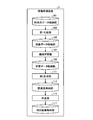
- FIG. 2 is a diagram illustrating a main processing flow according to the first embodiment.
- FIG. 3 is a diagram for explaining normalization of time series data.
- FIG. 4 is a diagram for explaining generation of an extended attractor.
- FIG. 5 is a diagram illustrating an example of the value of ⁇ .
- FIG. 6 is a diagram illustrating a processing flow of the extension vector generation processing.
- FIG. 7 is a diagram illustrating an example of a barcode diagram.
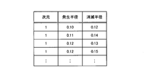
- FIG. 8 is a diagram illustrating an example of barcode data.
- FIG. 9 is a diagram for explaining the relationship between the barcode data and the Vetch series.
- FIG. 10 is a diagram illustrating an example of a persistent section.
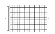
- FIG. 11 is a diagram for explaining the feature image.
- FIG. 12 is a diagram illustrating a main processing flow according to the first embodiment.
- FIG. 13 is a schematic diagram illustrating an example of a CNN according to the first embodiment.
- FIG. 14 is a diagram for explaining the relationship between labels and weight matrices.
- FIG. 15 is a diagram for explaining the calculation of statistics.
- FIG. 16 is a diagram for explaining the generation of the relevance vector.
- FIG. 17 is a diagram illustrating a main processing flow according to the first embodiment.
- FIG. 18 is a diagram showing a pattern for the first relation data.
- FIG. 19 is a diagram showing a pattern for the second relation data.
- FIG. 20 is a diagram illustrating a pattern for the third relational data and a pattern for the fourth relational data.
- FIG. 20 is a diagram illustrating a pattern for the third relational data and a pattern for the fourth relational data.
- FIG. 21 is a diagram illustrating a specific example of time-series data.
- FIG. 22 is a diagram illustrating a specific example of time-series data.
- FIG. 23 is a diagram illustrating a specific example of time-series data.
- FIG. 24 is a diagram illustrating a specific example of time-series data.
- FIG. 25 is a diagram illustrating a specific example of time-series data.
- FIG. 26 is a diagram illustrating a specific example of time-series data.
- FIG. 27 is a diagram illustrating a specific example of time-series data.
- FIG. 28 is a diagram illustrating a specific example of time-series data.
- FIG. 29 is a diagram illustrating the relationship between the degree of association and the contribution parameter.
- FIG. 29 is a diagram illustrating the relationship between the degree of association and the contribution parameter.
- FIG. 30 is a diagram illustrating a main processing flow according to the second embodiment.
- FIG. 31 is a diagram illustrating an example of a learning model according to the second embodiment.
- FIG. 32 is a functional block diagram of the information processing apparatus according to the third embodiment.
- FIG. 33 is a diagram illustrating a main process flow according to the third embodiment.
- FIG. 34 is a diagram illustrating an example of an input vector.
- FIG. 35 is a diagram illustrating a main processing flow according to the third embodiment.
- FIG. 36 is a diagram illustrating a main processing flow according to the third embodiment.
- FIG. 37 is a functional block diagram of the information processing apparatus according to the fourth embodiment.
- FIG. 38 is a diagram illustrating a main processing flow according to the fourth embodiment.
- FIG. 39 is a diagram for explaining calculation of the degree of association in the fourth embodiment.
- FIG. 40 is a functional block diagram of a computer.
- FIG. 1 is a functional block diagram of the information processing apparatus 1 according to the first embodiment.
- the information processing apparatus 1 includes a time-series data storage unit 101, a first generation unit 103, an image data storage unit 105, a machine learning unit 107, a learning data storage unit 109, a second generation unit 111, and a degree of association.
- a storage unit 113, a determination unit 115, and a determination result storage unit 117 are included.
- the first generation unit 103, the machine learning unit 107, the second generation unit 111, and the determination unit 115 are configured so that, for example, a program loaded in the memory 2501 illustrated in FIG. 40 is executed by a CPU (Central Processing Unit) 2503 illustrated in FIG. Realized by being executed.
- the time series data storage unit 101, the image data storage unit 105, the learning data storage unit 109, the relevance level storage unit 113, and the determination result storage unit 117 are stored in, for example, an HDD (Hard Disk Drive) 2505 or a memory 2501 shown in FIG. Provided.
- HDD Hard Disk Drive
- the first generation unit 103 executes processing based on the data stored in the time series data storage unit 101 and stores the processing result in the image data storage unit 105.
- the machine learning unit 107 executes processing based on the data stored in the image data storage unit 105 and stores the processing result in the learning data storage unit 109.
- the second generation unit 111 executes processing based on the data stored in the learning data storage unit 109 and stores the processing result in the relevance degree storage unit 113.
- the determination unit 115 executes processing based on the data stored in the association degree storage unit 113 and stores the processing result in the determination result storage unit 117.
- Data stored in the time-series data storage unit 101 includes, for example, biological data (time-series data such as heart rate, brain wave, pulse or body temperature), wearable sensor data (gyro sensor, acceleration sensor, geomagnetic sensor, etc.) Series data), financial data (time series data such as interest rates, prices, balance of payments or stock prices), natural environment data (time series data such as temperature, humidity or carbon dioxide concentration), or social data (labor statistics or population statistics) Etc.).
- biological data time-series data such as heart rate, brain wave, pulse or body temperature
- wearable sensor data gyro sensor, acceleration sensor, geomagnetic sensor, etc.
- financial data time series data such as interest rates, prices, balance of payments or stock prices
- natural environment data time series data such as temperature, humidity or carbon dioxide concentration
- social data labor statistics or population statistics
- time series data storage unit 101 stores a plurality of data sets including a plurality of time series data.
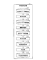
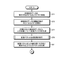
- FIG. 2 is a diagram illustrating a processing flow of processing executed by the information processing apparatus 1 according to the first embodiment.
- the first generation unit 103 identifies one data set among a plurality of data sets stored in the time-series data storage unit 101. Then, the first generation unit 103 translates each of the plurality of time-series data included in the identified data set so that the average of the values becomes 0 (FIG. 2: step S1).
- the first generation unit 103 performs normalization so that the amplitude widths of all time-series data for which the process of step S1 is executed are the same (step S3).
- the first generation unit 103 generates an extended attractor from a plurality of normalized time series data for each value of ⁇ (step S7).
- the first generation unit 103 stores the generated extended attractor in the memory 2501.
- ⁇ is a contribution parameter.
- x i (1 ⁇ i ⁇ (k + 2)) is a value of the first time series data
- y j (1 ⁇ j ⁇ (k + 2)) is a value of the second time series data.
- FIG. 4 is a diagram for explaining generation of an extended attractor.
- the generation of extended attractors is based on the Turkens embedding theorem.
- ⁇ 3 in the example of equation (2)
- the value of N and the value of ⁇ are not limited to the example of Expression (2).
- the contribution parameter ⁇ is, for example, a real number that satisfies 0 ⁇ ⁇ ⁇ 1, and is a parameter that adjusts the size of the time-series data value.
- the range of ⁇ may not be such a range.
- a plurality of values set at regular intervals are used.
- step S9 the 1st production
- the extended vector generation process will be described with reference to FIGS.
- the first generation unit 103 identifies one unprocessed value among the values of the contribution parameter ⁇ (FIG. 6: step S41).
- the first generation unit 103 reads the extended attractor for the value specified in step S41 from the memory 2501 (step S43).
- the first generation unit 103 generates barcode data from the extended attractor for each hole dimension (hereinafter referred to as hole dimension) by persistent homology processing (step S45).
- “Homology” is a technique for expressing the characteristics of an object by the number of holes of m (m ⁇ 0) dimensions.
- the “hole” referred to here is an element of a homology group.
- a zero-dimensional hole is a connected component, a one-dimensional hole is a hole (tunnel), and a two-dimensional hole is a cavity.
- the number of holes in each dimension is called the Betch number.
- the “persistent homology” is a technique for characterizing the transition of the m-dimensional hole in the target (here, the extended attractor), and the characteristics regarding the arrangement of the points can be examined by the persistent homology.
- each point in the object is gradually inflated into a spherical shape, and the time when each hole occurs (represented by the radius of the sphere at the time of occurrence) and the time of disappearance (by the radius of the sphere at the time of disappearance) Specified).
- a bar code diagram as shown in FIG. 7 can be generated by using the generation radius and the extinction radius of the hole.
- the horizontal axis represents the radius, and each line segment corresponds to one hole.
- the radius corresponding to the left end of the line segment is the generation radius of the hole, and the radius corresponding to the right end of the line segment is the disappearance radius of the hole.
- the line segment is called a persistent section. From such a bar code diagram, for example, it can be seen that there are two holes when the radius is 0.18.
- FIG. 8 shows an example of data for generating a barcode diagram (hereinafter referred to as barcode data).
- the barcode data includes a numerical value representing the hole dimension, the generation radius of the hole, and the disappearance radius of the hole.
- step S45 barcode data is generated for each hole dimension.
- the similar relationship between barcode data generated from a certain extended attractor and barcode data generated from another extended attractor is equivalent to the similar relationship between extended attractors. Therefore, the relationship between the extended attractor and the barcode data is a one-to-one relationship.
- the extended attractor is the same, the generated barcode data is the same. Conversely, if the barcode data is the same, the extended attractor is also the same. Further, when the extended attractors are similar, the barcode data is also similar, so that the conditions necessary for machine learning are satisfied. When the extended attractor is different, the bar code data is also different.
- the first generation unit 103 deletes the data of the persistent section whose length is less than the predetermined length from the barcode data generated in step S45 (step S47).
- the length of the persistent section is calculated by (annihilation radius ⁇ generation radius).
- the predetermined length is, for example, the length of time (hereinafter referred to as a block) obtained by dividing the time from when a zero-dimensional hole is generated until it disappears into K.
- the length is not limited to one block, and a plurality of blocks may have a predetermined length.
- the origin of the short time from occurrence to disappearance is mostly caused by noise. If the data of the persistent section whose length is less than the predetermined length is deleted, the influence of noise can be mitigated, so that the classification performance can be improved. However, it is assumed that the object of deletion is persistent section data having a dimension of 1 or more.
- step S47 If there is noise, a one-dimensional or more hole may occur for a short time. If the process of step S47 is executed, the data generated in both cases will be substantially the same, so the influence of noise can be removed.
- the similarity relationship between the barcode data after deletion is not strictly equivalent to the similarity relationship between the original barcode data. If the deletion is not performed, the similarity relationship is equivalent.
- the first generation unit 103 integrates the barcode data, and generates an extension vector from the integrated barcode data (step S48).
- An extension vector is a series of Betch numbers.
- the first generation unit 103 since the barcode data is generated for each hole dimension, the first generation unit 103 generates a single piece of barcode data by integrating a plurality of hole dimension barcode data.
- the series of the number of vetches is data indicating the relationship between the radius (that is, time) of the sphere and the number of the vetches in the persistent homology. With reference to FIG. 9, the relationship between the barcode data and the generated sequence of the number of vetches will be described.
- the upper graph is a graph generated from the barcode data, and the horizontal axis represents the radius.
- the lower graph is a graph generated from a series of the number of vetches, the vertical axis represents the number of vetches, and the horizontal axis represents time.
- the number of holes represents the number of holes.
- the number of holes existing at the radius corresponding to the broken line is 10, so in the lower graph, the number of holes is broken.
- the corresponding number of vetches is also ten.
- the number of vetches is counted for each block. Since the lower graph is a pseudo time-series data graph, the value on the horizontal axis itself is not meaningful.
- the same series can be obtained from the same barcode data. That is, the same sequence is obtained if the original set of points is the same. However, there are very rare cases where the same sequence can be obtained from different barcodes.
- this barcode data is data relating to holes of one or more dimensions.
- the persistent section p1 starts at time t1 and ends at time t2, and the persistent section p2 starts at time t2 and ends at time t3.
- the persistent section p4 starts at time t1 and ends at time t3. It is assumed that the persistent section p3 in both cases is exactly the same.
- the similarity between a series of vetch numbers generated from one barcode data and a series of vetch numbers generated from another barcode data is the same as the above-mentioned rare case. It is equivalent to the similarity between code data. From the above, although the definition of the distance between the data changes, the similarity relationship between the series of Betch numbers generated from the barcode data is almost equivalent to the similarity relationship between the original extended attractors.
- the first generation unit 103 determines whether there is an unprocessed value among the values of ⁇ (step S49). When there is an unprocessed value (step S49: Yes route), the process returns to step S41. If there is no unprocessed value (step S49: No route), the process returns to the caller.
- the barcode data generated by persistent homology processing is difficult to use as input for machine learning because the number of barcodes is not constant. Therefore, in the present embodiment, the barcode data is converted into a series of Betch numbers so that it can be used as an input for machine learning.
- the influence of noise can be removed.
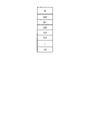
- the first generation unit 103 generates a feature image by combining the plurality of extension vectors generated in step S9 in the column direction in the order of the value of ⁇ (step S11).
- the generated feature image is stored in the image data storage unit 105. Then, the process proceeds to step S13 in FIG.
- FIG. 11 is a diagram illustrating an example of a feature image.
- a square figure represents a cell, and each cell stores the number of vetches that are elements of an expansion vector.
- One row corresponds to one extension vector. Therefore, in the example of FIG. 11, 11 extension vectors are combined, and the feature image corresponds to a matrix having 11 rows.
- the number of elements of the extension vector is 15, but the number is not limited.
- the machine learning unit 107 executes machine learning using CNN (Convolutional Neural Network) on the feature image generated in step S11 (step S13).
- CNN Convolutional Neural Network
- the machine learning unit 107 executes machine learning based on the feature image and its label.
- the machine learning unit 107 stores a result of machine learning (for example, an updated weight matrix) in the learning data storage unit 109.
- step S17 the processing after step S17 is executed.
- the second generation unit 111 identifies one unprocessed label among the plurality of labels related to the classification (step S17).
- FIG. 13 is a schematic diagram illustrating an example of the CNN according to the first embodiment.
- an operation such as convolution is executed with the feature image generated in step S11 as an input.
- the number of labels is 2, but the number of labels may be 3 or more.
- the second generation unit 111 reads, from the learning data storage unit 109, the elements of the weight matrix between the final feature layer and the identification layer for the label specified in step S17. Then, the second generation unit 111 calculates the absolute value of the read element (step S19).
- FIG. 14 is a diagram for explaining the relationship between labels and weight matrices.
- the CNN since the value of each cell of each unit in the final feature layer is multiplied by the weight in the weight matrix W n, the weight for each cell is read in step S19.
- the absolute value of the weight is also called activity.
- the second generation unit 111 calculates an absolute value statistic (for example, an average value or a maximum value) calculated in step S19 for each row of each weight matrix between the final feature layer and the identification layer (step S21). .
- an absolute value statistic for example, an average value or a maximum value
- FIG. 15 is a diagram for explaining the calculation of the statistics of activity. Since the image data of each unit of the final feature layer corresponds to the image data obtained by compressing the feature image generated in step S11, the vertical axis corresponds to the contribution parameter ⁇ . As will be described later, in the present embodiment, the correlation between a plurality of time-series data is specified based on the relationship between the contribution parameter ⁇ and the degree of relevance. Therefore, as shown in FIG. Is calculated. Therefore, for example, if the number of units of the final feature layer is 2, the absolute value statistic calculated in step S19 is calculated for each row of the two weight matrices. That is, a vector is generated for each unit of the final feature layer.
- the second generation unit 111 calculates, for each row, a statistic (for example, average, sum, or maximum value) of element values between units for the final feature layer vector. Then, the second generation unit 111 generates a vector having the calculated statistic as an element (step S23).
- a statistic for example, average, sum, or maximum value
- the second generation unit 111 generates a vector having the calculated statistic as an element (step S23).
- the value of each element of the vector generated in step S23 is handled as the degree of relevance.
- the degree of association is a value that represents the degree of influence of the cell on the target classification.
- FIG. 16 is a diagram for explaining generation of a relevance vector.
- the number of elements (that is, the number of rows) of the vector generated as a result of the processing in step S21 is the same between units. Therefore, in step S23, the value statistic is calculated as the relevance for each row, and one relevance vector is generated.
- the second generation unit 111 specifies the maximum value and minimum value of the relevance vector elements generated in step S23, and the positions (for example, element numbers) of the maximum and minimum values (step S25).
- the second generation unit 111 stores the relevance degree vector, the specified maximum value, minimum value, and positions of the maximum value and the minimum value in the relevance degree storage unit 113. The process proceeds to step S27 in FIG.
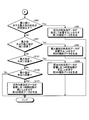
- the determination unit 115 reads information stored in the association degree storage unit 113. Then, the determination unit 115 determines whether the ratio of the maximum value to the minimum value is equal to or less than a predetermined value (FIG. 17: Step S27).
- the predetermined value is, for example, 1.2. That the ratio of the maximum value to the minimum value is equal to or less than the predetermined value means that the difference between the maximum value and the minimum value is relatively small.
- step S27 Yes route
- the determination unit 115 executes the following process. Specifically, the determination unit 115 generates first relational data indicating that both time series data independently affect the classification for the label specified in step S17 (step S28). Are stored in the determination result storage unit 117. Then, the process proceeds to step S37.
- FIG. 18 is a diagram showing a pattern for the first relational data.
- the vertical axis represents the degree of association
- the horizontal axis represents the contribution parameter ⁇ .
- the degree of relevance when the value of ⁇ is medium (if ⁇ is in the range of 0 ⁇ ⁇ ⁇ 1, when ⁇ is about 0.5) is also the same as the degree of relevance at both ends. Therefore, it is considered that there is no time correlation between the time series data.
- the determination unit 115 executes the following process. Specifically, the determination unit 115 determines whether the maximum value and the minimum value are located at the end of the relevance vector (step S29).
- the determination unit 115 executes the following processing. Specifically, the determination unit 115 generates second relational data indicating that the time-series data on the maximum value side affects the classification for the label specified in step S17 (step S30), The related data is stored in the determination result storage unit 117. Then, the process proceeds to step S37.
- FIG. 19A and FIG. 19B are diagrams showing patterns for the second relational data.
- the vertical axis represents the degree of association
- the horizontal axis represents the contribution parameter ⁇ .
- the determination unit 115 executes the following processing. Specifically, the determination unit 115 determines whether the maximum value is located at the center of the relevance vector (step S31).
- step S31 Yes route
- the determination unit 115 executes the following process. Specifically, the determination unit 115 determines the third relationship data indicating that both time series data affects the classification of the label specified in step S17 and that there is a correlation between the time series data. Generate (step S32), and store the third relation data in the determination result storage unit 117. Then, the process proceeds to step S37.
- FIG. 20 (a) is a diagram showing a pattern for the third relational data.
- the vertical axis represents the degree of association
- the horizontal axis represents the contribution parameter ⁇ . If the maximum value is located at the center of the relevance vector, the relevance values at both ends are considered to be relatively small. In that case, single time-series data may affect the classification of the target label. There is no. Since the maximum value is located at the center of the relevance vector, it is considered that there is a time correlation between the time series data.
- the determination unit 115 executes the following processing. Specifically, the determination unit 115 determines whether the minimum value is located at the center of the relevance vector (step S33).
- step S33: Yes route the determination unit 115 executes the following processing. Specifically, the determination unit 115 obtains fourth relation data indicating that both time series data influences the classification of the label specified in step S17 and that there is no correlation between the time series data. Generate (step S35), and store the fourth relation data in the determination result storage unit 117. On the other hand, when the minimum value is not located at the center of the relevance vector (step S33: No route), the process proceeds to step S37.
- FIG. 20B is a diagram showing a pattern for the fourth relational data.
- the vertical axis represents the degree of association
- the horizontal axis represents the contribution parameter ⁇ .
- the second generation unit 111 determines whether there is an unprocessed label (step S37). If there is an unprocessed label (step S37: Yes route), the process returns to step S17 in FIG. On the other hand, when there is no unprocessed label (step S37: No route), the process ends.
- the related data stored in the determination result storage unit 117 is displayed on the display device or transmitted to another terminal or the like, and is confirmed by the user.
- a feature image reflecting the features of each of a plurality of time-series data is generated.
- the feature image generated by the method of the present embodiment is suitable for machine learning.
- noise is removed in the feature image generation process, the accuracy of machine learning can be improved.
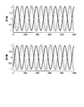
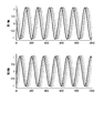
- FIGS. 21 to 28 show the first time-series data (the “first axis” time-series data in FIGS. 21 to 28), and the lower parts of FIGS. Eye time-series data (time-series data of “second axis” in FIGS. 21 to 28) is shown.
- Time series data having the same line type is included in the same data set.
- the time-series data of the thick line on the first axis in FIG. 21 is included in the same data set as the time-series data of the thick line on the second axis in FIG.
- label 1 is assigned when the combination of the time-series data of the first axis and the time-series data of the second axis is the combination shown in FIG. 21, and the time-series data of the first axis Label 2 is given when the combination with the time-series data of the second axis is the combination shown in FIG.
- the amplitude of the entire time series data on the first axis is about 1, and the amplitude of the time series data on the second axis is given randomly.
- the phase of the time series data on the first axis and the phase of the time series data on the second axis are randomly given.
- the amplitude of the entire time series data on the first axis is about 0.5, and the amplitude of the time series data on the second axis is randomly given.
- the phase of the time series data on the first axis and the phase of the time series data on the second axis are randomly given.
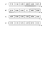
- FIG. 29A shows the relevance vector calculated by executing the processing of the present embodiment for the plurality of data sets shown in FIG. 21 and FIG.
- the ratio of the maximum value (0.138) to the minimum value (0.075) is larger than a predetermined value (1.2 here) and the value of ⁇ is the smallest.
- the maximum value of relevance appears and the value of ⁇ is the largest, the minimum value of relevance appears. Since this pattern corresponds to the pattern shown in FIG. 19A, only the time-series data on the first axis, which is the time-series data on the maximum value side, affects the classification (that is, the time-series data on the second axis). Is irrelevant to the classification). *
- label 1 is assigned when the combination of the time-series data of the first axis and the time-series data of the second axis is the combination shown in FIG.
- Label 2 is given when the combination with the time-series data of the second axis is the combination shown in FIG.
- the amplitude of the time-series data on the first axis is about 1
- the amplitude of the time-series data on the second axis is about 0.5. is there.
- the phase of the time series data on the first axis and the phase of the time series data on the second axis are randomly given.
- the amplitude of the time-series data on the first axis is about 0.5
- the amplitude of the time-series data on the second axis is about 1.
- the phase of the time series data on the first axis and the phase of the time series data on the second axis are randomly given.
- FIG. 29B shows a relevance vector calculated by executing the processing of the present embodiment for the plurality of data sets shown in FIGS.
- the maximum value of the degree of association is 0.105
- the minimum value of the degree of association is 0.091. Since the ratio of the maximum value to the minimum value is a predetermined value (1.2 here) or less, this pattern corresponds to the pattern shown in FIG. That is, it can be seen that both time-series data on the first axis and time-series data on the second axis affect the classification. In this case, it is possible to classify by at least one of the time series data.
- label 1 is assigned when the combination of the time-series data of the first axis and the time-series data of the second axis is the combination shown in FIG.
- Label 2 is given when the combination with the time-series data of the second axis is the combination shown in FIG.
- both the amplitude of the time-series data on the first axis and the amplitude of the time-series data on the second axis are about 1, or Both the amplitude of the time-series data on one axis and the amplitude of the time-series data on the second axis are about 0.5.
- the phase of the time series data on the first axis and the phase of the time series data on the second axis are randomly given.
- the amplitude of the time-series data on the first axis is about 1 and the amplitude of the time-series data on the second axis is about 0.5, or
- the amplitude of the time-series data on the first axis is about 0.5, and the amplitude of the time-series data on the second axis is about 1.
- the phase of the time series data on the first axis and the phase of the time series data on the second axis are randomly given.
- FIG. 29C shows a relevance vector calculated by executing the processing of the present embodiment for the plurality of data sets shown in FIG. 25 and FIG.
- the maximum value of the degree of association is 0.074
- the minimum value of the degree of association is 0.055. Since the ratio of the maximum value to the minimum value is larger than a predetermined value (here, 1.2) and the minimum value is located in a cell close to the center cell, this pattern corresponds to the pattern shown in FIG. there's a possibility that. That is, both the time-series data on the first axis and the time-series data on the second axis affect the classification (that is, both time-series data are necessary), but it is considered that they do not have time correlation.
- a predetermined value here, 1.2
- label 1 is assigned when the combination of the time-series data of the first axis and the time-series data of the second axis is the combination shown in FIG. 27, and the time-series data of the first axis Label 2 is given when the combination with the time-series data of the second axis is the combination shown in FIG.
- both the amplitude of the time-series data on the first axis and the amplitude of the time-series data on the second axis are about 1, and
- the phase of the time series data and the phase of the second axis time series data are the same.
- both the amplitude of the time-series data on the first axis and the amplitude of the time-series data on the second axis are about 1, and the time-series data of the second axis
- the phase is shifted by a half phase from the phase of the time-series data on the first axis.
- FIG. 29 (d) shows vectors of relevance calculated by executing the processing of the present embodiment for the plurality of data sets shown in FIG. 27 and FIG.
- the maximum value of the relevance level is 0.320
- the minimum value of the relevance level is 0.118. Since the ratio of the maximum value to the minimum value is larger than a predetermined value (1.2 in this case) and the maximum value is located in the center cell, this pattern corresponds to the pattern shown in FIG. That is, it can be seen that both the time-series data on the first axis and the time-series data on the second axis affect the classification (that is, both time-series data are necessary), and both have time correlation. .
- the present embodiment it is possible to specify the correlation between a plurality of time-series data for a target label. For example, if only one of the two time series data is found to affect the classification, the other time series data can be excluded from the acquisition and analysis of values, so that adverse effects on the classification can be avoided.
- the time and cost required for data acquisition and analysis can be reduced.
- the time series data can be selected from the viewpoint of the ease of data acquisition, etc. Acquisition time and cost can be reduced.
- the time and cost required for analysis can be reduced.
- machine learning using CNN is used and the relationship between cells in the feature image is taken into consideration, so that the accuracy of learning is increased compared to other embodiments described below. Will be able to.
- Emodiment 2 In the first embodiment, machine learning using CNN is executed on a feature image, but the machine learning method is not limited to CNN. Hereinafter, a method for directly learning feature images will be described with reference to FIGS. 30 and 31.
- the part different from the process of the first embodiment is the process after the terminal A, so only the process after the terminal A will be described below.
- Machine learning in the second embodiment is called machine learning using a single-layer learning model.
- the machine learning unit 107 performs machine learning using a single-layer learning model on the feature image generated in step S11 (FIG. 30: step S51).
- the machine learning unit 107 stores a result of machine learning (for example, an updated weight matrix) in the learning data storage unit 109.
- FIG. 31 is a diagram illustrating an example of a learning model according to the second embodiment.
- machine learning is performed on the value of each cell in the feature image.
- the value of each cell is multiplied by the weight for the identification layer.
- step S53 is executed after the processing of step S51 is executed for each of the plurality of data sets and it is confirmed that the machine learning has sufficiently progressed.
- the second generation unit 111 identifies one unprocessed label among the plurality of labels related to the classification (step S53).
- the second generation unit 111 extracts the weight for each cell in the feature image from the learning data storage unit 109 for the label specified in step S53 (step S55).
- the second generation unit 111 calculates the variance for each cell in the feature image (step S57). If the process up to step S11 is executed for a plurality of data sets, a plurality of feature images are generated, and therefore, for each cell, a variance is calculated from a plurality of values.
- the second generation unit 111 calculates the degree of association for each cell in the feature image based on the calculated variance and the absolute value of the extracted weight (step S59). For example, if the variance of the cell (x, y) is v x, y and the absolute value of the weight is w x, y , the second generation unit 111 sets the relevance of the cell (x, y) to v x , y * w Calculated as x, y .
- the second generation unit 111 generates a relevance vector by calculating a relevance statistic (for example, an average or maximum value) for each row (step S61), and stores the generated vector in the relevance storage unit 113. To do. Then, the process proceeds to step S27 in FIG.
- FIG. 32 is a functional block diagram of the information processing apparatus 1 according to the third embodiment.
- the information processing apparatus 1 includes a time-series data storage unit 101, a first generation unit 103, a vector data storage unit 119, a machine learning unit 107, a learning data storage unit 109, a second generation unit 111, and a degree of association.
- a storage unit 113, a determination unit 115, and a determination result storage unit 117 are included.
- the first generation unit 103, the machine learning unit 107, the second generation unit 111, and the determination unit 115 are realized, for example, by executing a program loaded in the memory 2501 illustrated in FIG. 40 by the CPU 2503 illustrated in FIG. Is done.
- the time series data storage unit 101, the vector data storage unit 119, the learning data storage unit 109, the relevance degree storage unit 113, and the determination result storage unit 117 are provided in, for example, the HDD 2505 or the memory 2501 illustrated in FIG.
- the first generation unit 103 executes processing based on the data stored in the time-series data storage unit 101, and stores the processing result in the vector data storage unit 119.
- the machine learning unit 107 executes processing based on the data stored in the vector data storage unit 119 and stores the processing result in the learning data storage unit 109.
- the second generation unit 111 executes processing based on the data stored in the learning data storage unit 109 and stores the processing result in the relevance degree storage unit 113.
- the determination unit 115 executes processing based on the data stored in the association degree storage unit 113 and stores the processing result in the determination result storage unit 117.
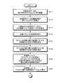
- FIG. 33 is a diagram illustrating a processing flow of processing executed by the information processing apparatus 1 according to the third embodiment.
- the first generation unit 103 identifies one data set among a plurality of data sets stored in the time-series data storage unit 101. Then, the first generation unit 103 translates each of the plurality of time-series data included in the identified data set so that the average value becomes 0 (FIG. 33: step S71).
- the first generation unit 103 performs normalization so that the amplitude widths of all time-series data for which the process of step S71 is performed are the same (step S73).
- the first generation unit 103 generates an extended attractor from a plurality of normalized time series data for each value of ⁇ (step S77).
- the first generation unit 103 stores the generated extended attractor in the memory 2501.
- the generation of the extended attractor is the same as that in the first embodiment.
- the first generation unit 103 executes extended vector generation processing using the extended attractor generated in step S77 (step S79).
- the extended vector generation process is the same as that described with reference to FIGS. 6 to 10, and the description thereof is omitted here.
- the first generation unit 103 generates an input vector by combining the plurality of extension vectors generated in step S79 in the row direction in the order of the value of ⁇ (step S81), and generates the input vector as a vector. Store in the data storage unit 119. Then, the process proceeds to step S83 in FIG.
- FIG. 34 is a diagram illustrating an example of an input vector.
- a square figure represents a vector element, and the number of vetches is stored in each element.
- a vector having seven elements corresponds to one extension vector. By concatenating such extension vectors, one input vector is generated.
- the machine learning unit 107 performs machine learning using the SVM on the input vector generated in step S81 (step S83).
- the machine learning unit 107 stores the machine learning result in the learning data storage unit 109.
- step S85 the processing of steps S71 to S83 is executed for one data set of the plurality of data sets has been shown, but actually, the processing is executed for each of the plurality of data sets. Then, after confirming that the machine learning has sufficiently progressed, the processes in and after step S85 are executed.
- the second generation unit 111 calculates an average value and a variance for each element of the input vector (step S85). If the process up to step S83 is executed for a plurality of data sets, a plurality of input vectors are generated, and thus the average and variance of values are calculated for each element.
- the second generation unit 111 generates a vector having the average value calculated in step S85 as the value of each element. Then, the second generation unit 111 calculates the generated vector classification score as a reference classification score using the result of machine learning using SVM (step S87). *
- the second generation unit 111 For each element of the vector generated in step S87, the second generation unit 111 changes the classification score when the value of only the element is changed to (average + variance) or (average ⁇ variance), and performs machine learning using SVM. Calculation is performed using the result (step S89).
- the second generation unit 111 calculates the relevance of each element as the difference between the classification score calculated in step S89 and the reference classification score (step S91), and stores the relevance in the relevance storage 113. Then, the process proceeds to step S93 in FIG.
- the determination unit 115 reads the information stored in the relevance degree storage unit 113. Then, the determination unit 115 determines whether the ratio of the maximum value to the minimum value is equal to or less than a predetermined value (FIG. 36: Step S93).
- the predetermined value is, for example, 1.2. That the ratio of the maximum value to the minimum value is equal to or less than the predetermined value means that the difference between the maximum value and the minimum value is relatively small.
- the determination unit 115 executes the following process. Specifically, the determination unit 115 generates first relationship data indicating that both time series data influences the classification independently (step S95), and the first relationship data is determined as the determination result storage unit 117. To store. Then, the process ends.
- the determination unit 115 executes the following processing. Specifically, the determination unit 115 determines whether the maximum value and the minimum value are located at the end of the relevance vector (step S97).
- the determination unit 115 executes the following processing. Specifically, the determination unit 115 generates second relationship data indicating that the time-series data on the maximum value side affects the classification (step S99), and the second relationship data is stored in the determination result storage unit 117. Store. Then, the process ends. *
- the determination unit 115 executes the following process. Specifically, the determination unit 115 determines whether the maximum value is located at the center of the relevance vector (step S101).
- the determination unit 115 executes the following processing. Specifically, the determination unit 115 generates third relationship data indicating that both time-series data have an influence on the classification and that there is a correlation between the time-series data (step S103). Are stored in the determination result storage unit 117. Then, the process ends.
- the determination unit 115 executes the following processing. Specifically, the determination unit 115 determines whether the minimum value is located at the center of the relevance vector (step S105).
- the determination unit 115 executes the following processing. Specifically, the determination unit 115 generates fourth relationship data indicating that both time-series data affect the classification and that there is no correlation between the time-series data (step S107). Are stored in the determination result storage unit 117. Then, the process ends. If the minimum value is not located at the center of the relevance vector (step S105: No route), the process ends. The related data stored in the determination result storage unit 117 is displayed on the display device or transmitted to another terminal or the like, and is confirmed by the user.
- machine learning using SVM can specify the correlation between a plurality of time-series data while improving the generalization performance.
- the relationship with the label is not described, but the processing may be executed for each label also in the third embodiment.
- the degree of association is calculated based on the result of machine learning.
- the degree of association is calculated by a method other than machine learning.
- FIG. 37 is a functional block diagram of the information processing apparatus 1 according to the fourth embodiment.
- the information processing apparatus 1 includes a time-series data storage unit 101, a first generation unit 103, a first data storage unit 121, a data processing unit 123, a second data storage unit 125, a second generation unit 111, The association degree storage unit 113, the determination unit 115, and the determination result storage unit 117 are included.
- the first generation unit 103, the data processing unit 123, the second generation unit 111, and the determination unit 115 are realized by a program loaded in the memory 2501 illustrated in FIG. 40 being executed by the CPU 2503 illustrated in FIG. Is done.
- the time-series data storage unit 101, the first data storage unit 121, the second data storage unit 125, the relevance degree storage unit 113, and the determination result storage unit 117 are provided, for example, in the HDD 2505 or the memory 2501 illustrated in FIG.
- the first generation unit 103 executes processing based on the data stored in the time-series data storage unit 101, and stores the processing result in the first data storage unit 121.
- the data processing unit 123 executes processing based on the data stored in the first data storage unit 121 and stores the processing result in the second data storage unit 125.
- the second generation unit 111 executes processing based on the data stored in the second data storage unit 125 and stores the processing result in the relevance degree storage unit 113.
- the determination unit 115 executes processing based on the data stored in the association degree storage unit 113 and stores the processing result in the determination result storage unit 117.
- FIG. 38 is a diagram illustrating a processing flow of processing executed by the information processing apparatus 1 according to the fourth embodiment. Here, the process will be described on the assumption that there are two labels.
- the first generation unit 103 identifies one data set among a plurality of data sets stored in the time-series data storage unit 101. Then, the first generation unit 103 translates each of the plurality of time-series data included in the identified data set so that the average value becomes 0 (FIG. 38: step S111).
- the first generation unit 103 performs normalization so that the amplitude widths of all time-series data for which the process of step S111 is performed are the same (step S113).
- the first generation unit 103 generates an extended attractor from a plurality of normalized time series data for each value of ⁇ (step S117).
- the first generation unit 103 stores the generated extended attractor in the memory 2501.
- the generation of the extended attractor is the same as that in the first embodiment.
- the first generation unit 103 executes extended vector generation processing using the extended attractor generated in step S117 (step S119).
- the extended vector generation process is the same as that described with reference to FIGS. 6 to 10, and the description thereof is omitted here.
- the data processing unit 123 calculates the average and variance of each element of the extension vector belonging to the label 1 classification among the plurality of extension vectors stored in the first data storage unit 121 by the process of step S119 (step S121). ).
- the data processing unit 123 calculates the average and variance of each element of the extension vector belonging to the classification of the label 2 among the plurality of extension vectors stored in the first data storage unit 121 by the process of step S119 (step S123).
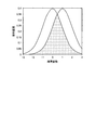
- the data processing unit 123 calculates, for each element, the area S of the portion where the two normal distributions overlap, assuming that the distribution for the label 1 and the distribution for the label 2 are normal distributions (step S125).
- the data processing unit 123 stores the area S for each element in the second data storage unit 125.
- step S125 for example, for two normal distributions as shown in FIG. 39, an area S that is an overlapping portion (hatched portion) is calculated for each element.
- the horizontal axis represents a random variable
- the vertical axis represents a probability density.
- the second generation unit 111 calculates the relevance level for the label 1 as (1-S) (step S127), and stores the relevance level for the label 1 in the relevance level storage unit 113.
- the relevance level for label 2 is similarly calculated as (1-S) and stored in the relevance level storage unit 113.
- the relevance level for label 1 is calculated as an average value of relevance levels for other labels. For example, when the number of labels is 3, the relevance level for label 1 is calculated as an average value of the relevance level for label 2 and the relevance level for label 3.
- the relevance vector is generated for label 1 and label 2 by the processing in step S127. Thereafter, the processing after the terminal E shown in FIG. 36 is executed for each label.
- the present invention is not limited to this.
- the functional block configuration of the information processing apparatus 1 described above may not match the actual program module configuration.
- the data configuration described above is an example, and it does not have to be the above configuration. Further, in the processing flow, the processing order can be changed if the processing result does not change. Further, it may be executed in parallel.
- the information processing apparatus 1 described above is a computer apparatus, and as shown in FIG. 40, a display controller 2507 connected to a memory 2501, a CPU 2503, an HDD 2505, a display device 2509, and a removable disk 2511.
- a drive device 2513, an input device 2515, and a communication control unit 2517 for connecting to a network are connected by a bus 2519.
- An operating system (OS: Operating System) and an application program for performing processing in this embodiment are stored in the HDD 2505, and are read from the HDD 2505 to the memory 2501 when executed by the CPU 2503.
- the CPU 2503 controls the display control unit 2507, the communication control unit 2517, and the drive device 2513 according to the processing content of the application program, and performs a predetermined operation.
- data in the middle of processing is mainly stored in the memory 2501, but may be stored in the HDD 2505.
- an application program for performing the above-described processing is stored in a computer-readable removable disk 2511 and distributed, and installed in the HDD 2505 from the drive device 2513.
- the HDD 2505 may be installed via a network such as the Internet and the communication control unit 2517.
- Such a computer apparatus realizes various functions as described above by organically cooperating hardware such as the CPU 2503 and the memory 2501 described above and programs such as the OS and application programs. .
- the data generation method includes (A) a persistence for a set of points represented by coordinates generated by a plurality of time-series data and the contribution rates of the plurality of time-series data. By the stent homology processing, a Betch number sequence corresponding to the contribution rate is generated. (B) A feature image is generated from a plurality of Betch number sequences generated for each of the plurality of contribution rates. (C) And a process of generating machine learning data in which classifications corresponding to a plurality of time-series data are associated.
- ⁇ Feature information suitable for machine learning for multiple time series data can be generated.
- the processing may further include generating (E) second data on the correlation between the plurality of time-series data regarding the specific classification based on the first data.
- Correlation of multiple time series data can be specified for a specific classification.
- the machine learning data may be machine learning data based on a convolutional neural network.
- (d1) based on the absolute value of the element of the weight matrix between the final feature layer and the identification layer included in the machine learning data, a plurality of degrees of association with a specific classification It may be calculated for each value of the contribution rate.
- the machine learning based on the convolutional neural network considers the positional relationship between the pixels included in the feature image as compared with other machine learning, so that the classification performance of the machine learning can be improved.
- the weight matrix between the final feature layer and the discrimination layer directly affects each classification in the discrimination layer, the degree of relevance for a specific classification in the discrimination layer can be calculated appropriately by executing the processing described above. It becomes like this.
- machine learning data may be machine learning data based on a single layer learning model.
- ⁇ Learning can be performed directly on the first data.
- each of the plurality of time-series data is based on the maximum value and minimum value of the relevance included in the first data, and the positions of the maximum value and the minimum value.
- Each of first relational data indicating that it influences a specific classification independently, second relational data indicating that any one of a plurality of time series data affects a specific classification, and each of a plurality of time series data Affects the specific classification, and the third relation data indicating that the plurality of time-series data have time correlation, or each of the plurality of time-series data affects the specific classification, and the plurality of times Fourth relational data indicating that the series data does not have time correlation may be generated.
- the first relation data is generated, and (e12) the maximum value and the minimum value are the first value.
- the second relationship data is generated, and (e13) the maximum value is located at the center of the relevance level column included in the first data
- the third relationship data may be generated, and (e14) the fourth relationship data may be generated when the minimum value is located at the center of the relevance column included in the first data.
- the plurality of time series data may be a plurality of normalized time series data.
- the data generation apparatus provides a persistence for a set of points represented by coordinates generated by (F) a plurality of time-series data and the contribution rates of the plurality of time-series data.
- a first generation unit (a first generation unit in the embodiment) that generates a vetch number sequence corresponding to a contribution rate by a stent homology process and generates a feature image from a plurality of vetch number sequences respectively generated for a plurality of contribution rates.
- the 1 generation unit 103 is an example of the first generation unit), (G) a second generation unit that generates machine learning data that associates feature images with classifications corresponding to a plurality of time-series data (
- the machine learning unit 107 according to the embodiment is an example of a second generation unit.
- a program for causing the processor to perform the processing according to the above method can be created.
- the program is, for example, a computer-readable storage medium such as a flexible disk, CD-ROM, magneto-optical disk, semiconductor memory, or hard disk. It is stored in a storage device.
- the intermediate processing result is temporarily stored in a storage device such as a main memory.
Landscapes
- Engineering & Computer Science (AREA)
- Theoretical Computer Science (AREA)
- Physics & Mathematics (AREA)
- Data Mining & Analysis (AREA)
- Software Systems (AREA)
- General Physics & Mathematics (AREA)
- Evolutionary Computation (AREA)
- General Engineering & Computer Science (AREA)
- Artificial Intelligence (AREA)
- Computer Vision & Pattern Recognition (AREA)
- Computing Systems (AREA)
- Mathematical Physics (AREA)
- Life Sciences & Earth Sciences (AREA)
- Medical Informatics (AREA)
- Computational Linguistics (AREA)
- Health & Medical Sciences (AREA)
- Biomedical Technology (AREA)
- Biophysics (AREA)
- General Health & Medical Sciences (AREA)
- Molecular Biology (AREA)
- Bioinformatics & Computational Biology (AREA)
- Evolutionary Biology (AREA)
- Bioinformatics & Cheminformatics (AREA)
- Information Retrieval, Db Structures And Fs Structures Therefor (AREA)
- Image Analysis (AREA)
Abstract
本データ生成方法は、複数の時系列データと、複数の時系列データそれぞれの寄与率とにより生成される座標で表された点の集合に対するパーシステントホモロジ処理により、寄与率に対応したベッチ数系列を生成し、複数の寄与率に対してそれぞれ生成された複数のベッチ数系列から特徴画像を生成し、特徴画像と、複数の時系列データに対応した分類とを対応付けた機械学習データを生成する処理を含む。
Description
本発明は、時系列データの処理技術に関する。
時系列データに対する機械学習が行われている。例えば、人に装着されたウエアラブルセンサにより取得された時系列データを学習データとし、かつ、時系列データが取得された時点における人の状態を教師データとして、学習モデルに対する機械学習をコンピュータに実行させる。そして、機械学習された学習モデルを利用し、新たな時系列データが取得された時点における人の状態をコンピュータに推定させる。
時系列データに対する機械学習に関して、或る文献は以下のような技術を開示する。具体的には、図形化手法に基づき時系列データが図形化され、図形化の結果に対して、位相幾何学に基づくデータ分析手法の一つである位相的データ解析(Topological Data Analysis)が実行される。そして、位相的データ解析の結果に対して、DNN(Deep Neural Network)を用いた機械学習が実行される。
但し、上記文献に記載の技術は、単一の時系列データに対する機械学習の技術であるので、複数の時系列データに対する機械学習に適した技術ではない。
富士通株式会社、"人々の安心安全な暮らしを支える新しいAI「時系列ディープラーニング」"、[online]、平成28年3月10日、[平成28年12月1日検索]、インターネット<URL:http://journal.jp.fujitsu.com/2016/03/10/01/>
本発明の目的は、1つの側面では、複数の時系列データに対する機械学習に適した特徴情報を生成することである。
一態様に係るデータ生成方法は、複数の時系列データと、複数の時系列データそれぞれの寄与率とにより生成される座標で表された点の集合に対するパーシステントホモロジ処理により、寄与率に対応したベッチ数系列を生成し、複数の寄与率に対してそれぞれ生成された複数のベッチ数系列から特徴画像を生成し、特徴画像と、複数の時系列データに対応した分類とを対応付けた機械学習データを生成する処理を含む。
1つの側面では、複数の時系列データに対する機械学習に適した特徴情報を生成できる。
[実施の形態1]
図1は、第1の実施の形態の情報処理装置1の機能ブロック図である。情報処理装置1は、時系列データ格納部101と、第1生成部103と、画像データ格納部105と、機械学習部107と、学習データ格納部109と、第2生成部111と、関連度格納部113と、判定部115と、判定結果格納部117とを含む。
図1は、第1の実施の形態の情報処理装置1の機能ブロック図である。情報処理装置1は、時系列データ格納部101と、第1生成部103と、画像データ格納部105と、機械学習部107と、学習データ格納部109と、第2生成部111と、関連度格納部113と、判定部115と、判定結果格納部117とを含む。
第1生成部103、機械学習部107、第2生成部111および判定部115は、例えば、図40に示したメモリ2501にロードされたプログラムが図40に示したCPU(Central Processing Unit)2503により実行されることで実現される。時系列データ格納部101、画像データ格納部105、学習データ格納部109、関連度格納部113および判定結果格納部117は、例えば、図40に示したHDD(Hard Disk Drive)2505又はメモリ2501に設けられる。
第1生成部103は、時系列データ格納部101に格納されているデータに基づき処理を実行し、処理結果を画像データ格納部105に格納する。機械学習部107は、画像データ格納部105に格納されているデータに基づき処理を実行し、処理結果を学習データ格納部109に格納する。第2生成部111は、学習データ格納部109に格納されているデータに基づき処理を実行し、処理結果を関連度格納部113に格納する。判定部115は、関連度格納部113に格納されているデータに基づき処理を実行し、処理結果を判定結果格納部117に格納する。
時系列データ格納部101に格納されているデータは、例えば、生体データ(心拍数、脳波、脈拍或いは体温などの時系列データ)、ウエアラブルセンサのデータ(ジャイロセンサ、加速度センサ或いは地磁気センサなどの時系列データ)、金融データ(金利、物価、国際収支或いは株価などの時系列データ)、自然環境のデータ(気温、湿度或いは二酸化炭素濃度などの時系列データ)、又は社会データ(労働統計或いは人口統計などのデータ)等である。但し、時系列データは、少なくとも以下のルールに従って変化するデータであるとする。

例えば、不規則な時系列データ又は手書き文字の軌跡などの人為的な動きに関するデータは、本実施の形態の対象外であるとする。また、時系列データ格納部101には、複数の時系列データを含むデータセットが複数格納されているとする。
図2は、第1の実施の形態の情報処理装置1が実行する処理の処理フローを示す図である。
第1生成部103は、時系列データ格納部101に格納されている複数のデータセットのうち1つのデータセットを特定する。そして、第1生成部103は、特定したデータセットに含まれる複数の時系列データの各々を、値の平均が0になるように平行移動する(図2:ステップS1)。
第1生成部103は、ステップS1の処理が実行された全時系列データの振幅の幅が同じになるように正規化を実行する(ステップS3)。
複数の時系列データが異なる種類の時系列データである場合には軸のスケールが異なるので、時系列データの生の値をそのまま利用することは問題である。例えば図3に示すように、時系列データt1の値の変動が時系列データt2の値の変動より大きい場合であっても、分類に与える影響に関しても時系列データt1の方が大きいとは限らないので、軸のスケールが異なっていると誤った学習が行われる可能性がある。そこで、ステップS3の処理により軸のスケールを一致させることで、この問題を解消することができる。
第1生成部103は、αの各値について、正規化された複数の時系列データから拡張アトラクタを生成する(ステップS7)。第1生成部103は、生成した拡張アトラクタをメモリ2501に格納する。
例えば、時系列データの数が2つである場合には以下のような拡張アトラクタが生成される。
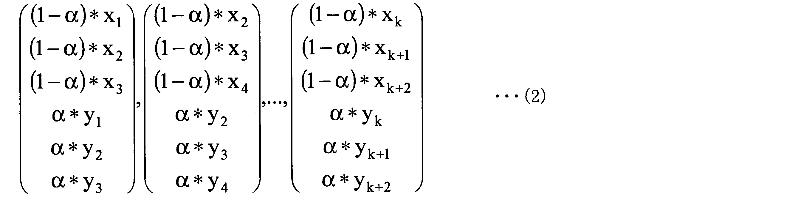
αは寄与パラメータである。xi(1≦i≦(k+2))は第1の時系列データの値であり、yj(1≦j≦(k+2))は第2の時系列データの値である。
図4は、拡張アトラクタの生成について説明するための図である。拡張アトラクタの生成はターケンスの埋め込み定理に基づく。第1の時系列データから取り出されたN個(Nは埋め込み次元である。式(2)の例ではN=3)の値に(1-α)が乗じられ、第2の時系列データから取り出されたN個の値にαが乗じられ、それらの値は1つの点の座標の成分になる。式(2)の例ではτ=1であるため1つおきに要素が取り出されている。但し、Nの値およびτの値は式(2)の例には限られない。
寄与パラメータαは、例えば、0≦α≦1を満たす実数であり、時系列データの値の大きさを調整するパラメータである。但し、αの範囲はこのような範囲でなくてもよい。本実施の形態においては、例えば図5に示すように、一定の間隔で設定された複数の値が使用される。
そして、第1生成部103は、ステップS7において生成された拡張アトラクタを用いて、拡張ベクトル生成処理を実行する(ステップS9)。拡張ベクトル生成処理については、図6乃至図10を用いて説明する。
第1生成部103は、寄与パラメータαの値のうち未処理の値を1つ特定する(図6:ステップS41)。
第1生成部103は、ステップS41において特定した値についての拡張アトラクタを、メモリ2501から読み出す(ステップS43)。
第1生成部103は、パーシステントホモロジ処理によって、拡張アトラクタからバーコードデータを穴の次元(以下、穴次元と呼ぶ)毎に生成する(ステップS45)。
「ホモロジ」とは、対象の特徴をm(m≧0)次元の穴の数によって表現する手法である。ここで言う「穴」とはホモロジ群の元のことであり、0次元の穴は連結成分であり、1次元の穴は穴(トンネル)であり、2次元の穴は空洞である。各次元の穴の数はベッチ数と呼ばれる。
「パーシステントホモロジ」とは、対象(ここでは、拡張アトラクタ)におけるm次元の穴の遷移を特徴付けるための手法であり、パーシステントホモロジによって点の配置に関する特徴を調べることができる。この手法においては、対象における各点が球状に徐々に膨らまされ、その過程において各穴が発生した時刻(発生時の球の半径で表される)と消滅した時刻(消滅時の球の半径で表される)とが特定される。
穴の発生半径と消滅半径とを使用することで、例えば図7に示すようなバーコード図を生成することができる。図7において、横軸は半径を表し、各線分は1つの穴に対応する。線分の左端に対応する半径は穴の発生半径であり、線分の右端に対応する半径は穴の消滅半径である。線分はパーシステント区間と呼ばれる。このようなバーコード図から、例えば半径が0.18である時には2つの穴が存在するということがわかる。
図8に、バーコード図を生成するためのデータ(以下、バーコードデータと呼ぶ)の一例を示す。図8の例では、穴次元を表す数値と、穴の発生半径と、穴の消滅半径とがバーコードデータに含まれる。ステップS45において、バーコードデータは穴次元毎に生成される。
以上のような処理を実行すれば、或る拡張アトラクタから生成されるバーコードデータと他の拡張アトラクタから生成されるバーコードデータとの類似関係は、拡張アトラクタ間の類似関係と等価である。よって、拡張アトラクタとバーコードデータとの関係は1対1の関係である。
すなわち、拡張アトラクタが同じであれば、生成されるバーコードデータは同じである。逆に、バーコードデータが同じであれば、拡張アトラクタも同じである。また、拡張アトラクタが類似している場合にはバーコードデータも類似するため、機械学習に必要な条件が満たされる。拡張アトラクタが異なる場合には、バーコードデータも異なる。
なお、パーシステントホモロジの詳細については、例えば「平岡裕章、『タンパク質構造とトポロジー パーシステントホモロジー群入門』、共立出版」を参照されたい。
図6の説明に戻り、第1生成部103は、長さが所定長未満であるパーシステント区間のデータを、ステップS45において生成されたバーコードデータから削除する(ステップS47)。なお、パーシステント区間の長さは、(消滅半径-発生半径)によって算出される。所定長は、例えば、0次元の穴が発生してから消滅するまでの時間をK等分した時間(以下、ブロックと呼ぶ)の長さである。但し、1ブロックの長さに限られるわけではなく、複数ブロックの長さを所定長としてもよい。
発生から消滅までの時間が短い元は、ノイズによって発生するものがほとんどである。長さが所定長未満であるパーシステント区間のデータを削除すれば、ノイズの影響を緩和することができるので、分類性能を向上させることができるようになる。但し、削除の対象は次元が1以上であるパーシステント区間のデータであるとする。
ノイズが発生した場合においては、僅かな時間だけ1次元以上の穴が発生することがある。ステップS47の処理を実行すれば、両ケースにおいて生成されるデータはほぼ同じになるので、ノイズの影響を取り除くことができるようになる。
なお、長さが所定長未満であるパーシステント区間のデータが削除されるので、削除後のバーコードデータ間の類似関係は、元のバーコードデータ間の類似関係と厳密には等価ではない。削除が行われない場合には、類似関係は等価である。
図6の説明に戻り、第1生成部103は、バーコードデータを統合し、統合されたバーコードデータから拡張ベクトルを生成する(ステップS48)。拡張ベクトルはベッチ数の系列である。
上で述べたように、バーコードデータは穴次元毎に生成されるので、第1生成部103は、複数の穴次元のバーコードデータを統合することで1塊のバーコードデータを生成する。ベッチ数の系列は、パーシステントホモロジにおける球の半径(すなわち時間)とベッチ数との関係を示すデータである。図9を用いて、バーコードデータと生成されるベッチ数の系列との関係について説明する。上段のグラフはバーコードデータから生成されるグラフであり、横軸が半径を表す。下段のグラフはベッチ数の系列から生成されるグラフであり、縦軸はベッチ数を表し、横軸は時間を表す。上で述べたように、ベッチ数は穴の数を表しており、例えば上段のグラフにおいて破線に対応する半径の時には存在している穴の数が10であるので、下段のグラフにおいては破線に対応するベッチ数も10である。ベッチ数は、ブロック毎に計数される。なお、下段のグラフは疑似的な時系列データのグラフであるので、横軸の値自体が意味を持つわけではない。
基本的には、同じバーコードデータからは同じ系列が得られる。すなわち、元の点の集合が同じであれば同じ系列が得られる。但し、異なるバーコードから同じ系列が得られるケースが極めて稀に発生する。
例えば図10に示すようなバーコードデータを考える。このバーコードデータは1以上の次元の穴に関するデータであるとする。図10(a)のケースにおいては、パーシステント区間p1が時刻t1で開始し、かつ、時刻t2で終了し、パーシステント区間p2が時刻t2で開始し、かつ、時刻t3で終了する。一方、図10(b)のケースにおいては、パーシステント区間p4が時刻t1で開始し、かつ、時刻t3で終了する。両ケースにおけるパーシステント区間p3は全く同じであるとする。
このような場合、両ケースにおけるバーコードデータからは全く同じ系列が得られるので、両ケースを区別することができない。しかし、このような現象が発生する可能性は極めて低い。また、両ケースの点の集合は元々似ており、機械学習による分類に与える影響が極めて小さいので、上記のような現象が発生しても問題は無い。
従って、或るバーコードデータから生成されるベッチ数の系列と、別のバーコードデータから生成されるベッチ数の系列との類似関係は、上で述べた稀なケースが発生しなければ、バーコードデータ間の類似関係と等価である。以上から、データ間の距離の定義は変わるものの、バーコードデータから生成されるベッチ数の系列間の類似関係は、元の拡張アトラクタ間の類似関係とほぼ等価である。
図6の説明に戻り、第1生成部103は、αの値のうち未処理の値が有るか判定する(ステップS49)。未処理の値が有る場合(ステップS49:Yesルート)、ステップS41の処理に戻る。未処理の値が無い場合(ステップS49:Noルート)、処理は呼び出し元に戻る。
以上のように、パーシステントホモロジ処理を実行すれば、拡張アトラクタにおける点の位置関係を、バーコードデータに反映することができる。パーシステントホモロジ処理によって生成されたバーコードデータは、バーコードの本数が一定ではないため、そのままでは機械学習の入力とすることが難しい。そこで本実施の形態においては、バーコードデータをベッチ数の系列に変換することで、機械学習の入力とすることを可能にしている。
また、上で述べたように、本実施の形態によればノイズの影響を取り除くことができる。
図2の説明に戻り、第1生成部103は、ステップS9において生成された複数の拡張ベクトルを、αの値の大きさの順に列方向に結合することで特徴画像を生成し(ステップS11)、生成した特徴画像を画像データ格納部105に格納する。そして処理は端子Aを介して図12のステップS13に移行する。
図11は、特徴画像の一例を示す図である。正方形の図形はセルを表し、各セルには拡張ベクトルの要素であるベッチ数が格納される。1つの行が1つの拡張ベクトルに対応する。従って、図11の例においては、11個の拡張ベクトルが結合されており、特徴画像は11の行を有する行列に相当する。図11においては拡張ベクトルの要素の数が15であるが、数に限定は無い。
図12の説明に移行し、機械学習部107は、ステップS11において生成された特徴画像に対して、CNN(Convolutional Neural Network)を用いた機械学習を実行する(ステップS13)。ここでは、機械学習部107は、特徴画像とそのラベルとに基づく機械学習を実行する。機械学習部107は、機械学習の結果(例えば更新後の重み行列等)を学習データ格納部109に格納する。
なお、説明を簡単にするため複数のデータセットのうち1つのデータセットについてステップS1乃至S13の処理が実行される例を示したが、実際には、複数のデータセットの各々について処理が実行される。そして、機械学習が十分に進んだことが確認されたうえで、ステップS17以降の処理が実行される。
第2生成部111は、分類に関する複数のラベルのうち未処理のラベルを1つ特定する(ステップS17)。
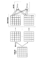
図13は、第1の実施の形態におけるCNNの一例を示す模式図である。第1の実施の形態の機械学習においては、ステップS11において生成された特徴画像を入力として、畳み込み等の演算が実行される。最終特徴層と識別層との間は全結合である。図13の例においてはラベルの数は2であるが、ラベルの数が3以上であってもよい。
第2生成部111は、ステップS17において特定したラベルについて、最終特徴層と識別層との間の重み行列の要素を、学習データ格納部109から読み出す。そして、第2生成部111は、読み出した要素の絶対値を算出する(ステップS19)。
図14は、ラベルと重み行列との関係を説明するための図である。CNNにおいては、最終特徴層における各ユニットの各セルの値に重み行列Wnにおける重みが乗じられるので、ステップS19においては各セルについての重みが読み出される。なお、重みの絶対値は活性度とも呼ばれる。
第2生成部111は、最終特徴層と識別層との間の各重み行列の各行について、ステップS19において算出した絶対値の統計量(例えば、平均値又は最大値)を算出する(ステップS21)。
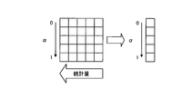
図15は、活性度の統計量の算出について説明するための図である。最終特徴層の各ユニットの画像データは、ステップS11において生成された特徴画像を圧縮した画像データに相当するので、縦軸は寄与パラメータαに対応している。後述のように、本実施の形態においては寄与パラメータαと関連度との関係に基づき複数の時系列データの相関関係が特定されるので、図15に示すように、αの各値について統計量が算出される。従って、例えば最終特徴層のユニット数が2であれば、2つの重み行列それぞれの各行について、ステップS19において算出された絶対値の統計量が算出される。すなわち、最終特徴層の各ユニットについてベクトルが生成される。
第2生成部111は、最終特徴層のベクトルについて、ユニット間で要素の値の統計量(例えば、平均、総和又は最大値)を行毎に算出する。そして、第2生成部111は、算出した統計量を要素とするベクトルを生成する(ステップS23)。第1の実施の形態においては、ステップS23において生成されたベクトルの各要素の値を関連度として取り扱う。関連度とは、対象の分類に対してセルが及ぼす影響の度合いを表す値である。
図16は、関連度のベクトルの生成について説明するための図である。ステップS21の処理の結果として生成されたベクトルの要素数(すなわち行数)はユニット間で同一である。従って、ステップS23においては、値の統計量が行毎に関連度として算出され、関連度のベクトルが1つ生成される。
第2生成部111は、ステップS23において生成した関連度のベクトルの要素の最大値、最小値、並びに最大値および最小値の位置(例えば要素番号)を特定する(ステップS25)。第2生成部111は、関連度のベクトルと、特定した最大値、最小値、並びに最大値および最小値の位置とを関連度格納部113に格納する。処理は端子Bを介して図17のステップS27に移行する。
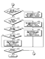
図17の説明に移行し、判定部115は、関連度格納部113に格納されている情報を読み出す。そして、判定部115は、最小値に対する最大値の割合が所定値以下であるか判定する(図17:ステップS27)。所定値とは、例えば1.2である。最小値に対する最大値の割合が所定値以下であることは、最大値と最小値との差が比較的小さいことを意味する。
最小値に対する最大値の割合が所定値以下である場合(ステップS27:Yesルート)、判定部115は、以下の処理を実行する。具体的には、判定部115は、ステップS17において特定されたラベルについての分類に両方の時系列データが独立して影響することを示す第1の関係データを生成し(ステップS28)、第1の関係データを判定結果格納部117に格納する。そして処理はステップS37に移行する。
図18は、第1の関係データについてのパターンを示す図である。図18において、縦軸は関連度を表し、横軸は寄与パラメータαを表す。最小値に対する最大値の割合が所定値以下である場合には、αの値が比較的小さいとき(すなわち、一方の時系列データの値に乗じられる寄与パラメータの値が比較的大きい場合)と、αの値が比較的大きいとき(すなわち、他方の時系列データの値に乗じられる寄与パラメータの値が比較的大きい場合)とで、関連度が同程度になる。このような場合には、対象のラベルについての分類に両方の時系列データが影響を及ぼしていると考えられる。そして、αの値の大きさが中程度であるとき(仮にαの範囲が0≦α≦1であれば、αが約0.5であるとき)の関連度も両端の関連度と同程度であるので、時系列データの間に時間相関が無いと考えられる。
一方、最小値に対する最大値の割合が所定値以下ではない場合(ステップS27:Noルート)、判定部115は、以下の処理を実行する。具体的には、判定部115は、最大値および最小値が関連度のベクトルの端に位置するか判定する(ステップS29)。
最大値および最小値が関連度のベクトルの端に位置する場合(ステップS29:Yesルート)、判定部115は、以下の処理を実行する。具体的には、判定部115は、ステップS17において特定されたラベルについての分類に最大値側の時系列データが影響することを示す第2の関係データを生成し(ステップS30)、第2の関係データを判定結果格納部117に格納する。そして処理はステップS37に移行する。
図19(a)及び図19(b)は、第2の関係データについてのパターンを示す図である。図19(a)及び図19(b)において、縦軸は関連度を表し、横軸は寄与パラメータαを表す。最大値および最小値が関連度のベクトルの端に位置する場合、関連度と寄与パラメータαとの関係はおおよそ図19(a)又は図19(b)に示すような関係である。このような場合には、対象のラベルについての分類には、関連度の最大値側の時系列データが影響すると考えられる。そして、時系列データ間の時間相関は無いと考えられる。
一方、最大値および最小値の少なくともいずれかが関連度のベクトルの端に位置しない場合(ステップS29:Noルート)、判定部115は、以下の処理を実行する。具体的には、判定部115は、最大値が関連度のベクトルの中央に位置するか判定する(ステップS31)。
最大値が関連度のベクトルの中央に位置する場合(ステップS31:Yesルート)、判定部115は、以下の処理を実行する。具体的には、判定部115は、ステップS17において特定されたラベルについての分類に両方の時系列データが影響し、かつ、時系列データ間に相関関係があることを示す第3の関係データを生成し(ステップS32)、第3の関係データを判定結果格納部117に格納する。そして処理はステップS37に移行する。
図20(a)は、第3の関係データについてのパターンを示す図である。図20(a)において、縦軸は関連度を表し、横軸は寄与パラメータαを表す。最大値が関連度のベクトルの中央に位置する場合、両端の関連度の値が比較的小さくなると考えられ、その場合には対象のラベルについての分類に対して単独の時系列データが影響することはない。そして、最大値が関連度のベクトルの中央に位置することから、時系列データ間に時間相関が有ると考えられる。
一方、最大値が関連度のベクトルの中央に位置しない場合(ステップS31:Noルート)、判定部115は、以下の処理を実行する。具体的には、判定部115は、最小値が関連度のベクトルの中央に位置するか判定する(ステップS33)。
最小値が関連度のベクトルの中央に位置する場合(ステップS33:Yesルート)、判定部115は、以下の処理を実行する。具体的には、判定部115は、ステップS17において特定されたラベルについての分類に両方の時系列データが影響し、かつ、時系列データ間に相関関係が無いことを示す第4の関係データを生成し(ステップS35)、第4の関係データを判定結果格納部117に格納する。一方、最小値が関連度のベクトルの中央に位置しない場合(ステップS33:Noルート)、処理はステップS37に移行する。
図20(b)は、第4の関係データについてのパターンを示す図である。図20(b)において、縦軸は関連度を表し、横軸は寄与パラメータαを表す。最小値が関連度のベクトルの中央に位置する場合、両端の関連度の値が比較的大きくなると考えられ、その場合には対象のラベルについての分類に対して時系列データ単独で影響する。そして、最小値が関連度のベクトルの中央に位置することから、時系列データ間に時間相関が無いと考えられる。
第2生成部111は、未処理のラベルが有るか判定する(ステップS37)。未処理のラベルが有る場合(ステップS37:Yesルート)、処理は端子Cを介して図12のステップS17に戻る。一方、未処理のラベルが無い場合(ステップS37:Noルート)、処理は終了する。なお、判定結果格納部117に格納された関係データは表示装置に表示され又は他の端末等に送信され、ユーザにより確認される。
以上のように、本実施の形態によれば、複数の時系列データそれぞれの特徴が反映された特徴画像が生成されるようになる。複数の時系列データそのものを機械学習の入力とすることは難しいが、本実施の形態の方法により生成された特徴画像は機械学習に適している。また、特徴画像の生成過程においてノイズが取り除かれるため、機械学習の精度を高めることが可能である。
以下では、時系列データ間の相関関係の特定について、図21乃至図29に示した具体例を用いて説明を追加する。
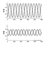
図21乃至図28の上段には1つ目の時系列データ(図21乃至図28における「第1軸」の時系列データ)が示されており、図21乃至図28の下段には2つ目の時系列データ(図21乃至図28における「第2軸」の時系列データ)が示されている。線種が同じである時系列データは同じデータセットに含まれる。例えば、図21の第1軸の太線の時系列データは、図21の第2軸の太線の時系列データと同じデータセットに含まれる。
まず、図21、図22及び図29(a)を用いて、第1の例について説明する。第1の例においては、第1軸の時系列データと第2軸の時系列データとの組合せが図21に示した組み合わせである場合にラベル1が付与され、第1軸の時系列データと第2軸の時系列データとの組合せが図22に示した組み合わせである場合にラベル2が付与される。
より具体的には、図21に示すように、第1軸の全時系列データの振幅は約1であり、第2軸の時系列データの振幅はランダムに与えられている。第1軸の時系列データの位相及び第2軸の時系列データの位相はランダムに与えられている。
また、図22に示すように、第1軸の全時系列データの振幅は約0.5であり、第2軸の時系列データの振幅はランダムに与えられている。第1軸の時系列データの位相及び第2軸の時系列データの位相はランダムに与えられている。
図21及び図22に示した複数のデータセットについて本実施の形態の処理を実行することで算出された関連度のベクトルを図29(a)に示す。図29(a)に示した例においては、最小値(0.075)に対する最大値(0.138)の割合が所定値(ここでは1.2)より大きく、αの値が最も小さい場合に関連度の最大値が出現し、かつ、αの値が最も大きい場合に関連度の最小値が出現している。このパターンは図19(a)に示したパターンに相当するので、最大値側の時系列データである第1軸の時系列データのみが分類に影響を及ぼす(すなわち、第2軸の時系列データは分類に無関係)ことがわかる。
図23、図24及び図29(b)を用いて、第2の例について説明する。第2の例においては、第1軸の時系列データと第2軸の時系列データとの組合せが図23に示した組み合わせである場合にラベル1が付与され、第1軸の時系列データと第2軸の時系列データとの組合せが図24に示した組み合わせである場合にラベル2が付与される。
より具体的には、図23に示すように、各データセットについて、第1軸の時系列データの振幅は約1であり、かつ、第2軸の時系列データの振幅は約0.5である。第1軸の時系列データの位相及び第2軸の時系列データの位相はランダムに与えられている。
また、図24に示すように、各データセットにおいて、第1軸の時系列データの振幅は約0.5であり、かつ、第2軸の時系列データの振幅は約1である。第1軸の時系列データの位相及び第2軸の時系列データの位相はランダムに与えられている。
図23及び図24に示した複数のデータセットについて本実施の形態の処理を実行することで算出された関連度のベクトルを図29(b)に示す。図29(b)に示した例においては、関連度の最大値は0.105であり、関連度の最小値は0.091である。最小値に対する最大値の割合が所定値(ここでは1.2)以下であるので、このパターンは図18に示したパターンに相当する。つまり、第1軸の時系列データおよび第2軸の時系列データの両方が分類に影響を及ぼすことがわかる。この場合、少なくともいずれかの時系列データによって分類をすることが可能である。
図25、図26及び図29(c)を用いて、第3の例について説明する。第3の例においては、第1軸の時系列データと第2軸の時系列データとの組合せが図25に示した組み合わせである場合にラベル1が付与され、第1軸の時系列データと第2軸の時系列データとの組合せが図26に示した組み合わせである場合にラベル2が付与される。
より具体的には、図25に示すように、各データセットについて、第1軸の時系列データの振幅と第2軸の時系列データの振幅との両方が約1であるか、又は、第1軸の時系列データの振幅と第2軸の時系列データの振幅との両方が約0.5である。第1軸の時系列データの位相及び第2軸の時系列データの位相はランダムに与えられている。
また、図26に示すように、各データセットについて、第1軸の時系列データの振幅が約1であり、かつ、第2軸の時系列データの振幅が約0.5であるか、又は、第1軸の時系列データの振幅が約0.5であり、かつ、第2軸の時系列データの振幅が約1である。第1軸の時系列データの位相及び第2軸の時系列データの位相はランダムに与えられている。
図25及び図26に示した複数のデータセットについて本実施の形態の処理を実行することで算出された関連度のベクトルを図29(c)に示す。図29(c)に示した例においては、関連度の最大値は0.074であり、関連度の最小値は0.055である。最小値に対する最大値の割合が所定値(ここでは1.2)より大きく、かつ、最小値が中央のセルに近いセルに位置するので、このパターンは図20(b)に示したパターンに相当する可能性がある。つまり、第1軸の時系列データおよび第2軸の時系列データの両方が分類に影響を及ぼす(すなわち、両方の時系列データが必要である)が両者は時間相関を有しないと考えられる。
図27、図28及び図29(d)を用いて、第4の例について説明する。第4の例においては、第1軸の時系列データと第2軸の時系列データとの組合せが図27に示した組み合わせである場合にラベル1が付与され、第1軸の時系列データと第2軸の時系列データとの組合せが図28に示した組み合わせである場合にラベル2が付与される。
より具体的には、図27に示すように、各データセットについて、第1軸の時系列データの振幅と第2軸の時系列データの振幅との両方が約1であり、第1軸の時系列データの位相と第2軸の時系列データの位相とが同じである。
また、図28に示すように、各データセットについて、第1軸の時系列データの振幅と第2軸の時系列データの振幅との両方が約1であり、第2軸の時系列データの位相は第1軸の時系列データの位相と半位相分ずれている。
図27及び図28に示した複数のデータセットについて本実施の形態の処理を実行することで算出した関連度のベクトルを図29(d)に示す。図29(d)に示した例においては、関連度の最大値は0.320であり、関連度の最小値は0.118である。最小値に対する最大値の割合が所定値(ここでは1.2)より大きく、かつ、最大値が中央のセ ルに位置するので、このパターンは図20(a)に示したパターンに相当する。つまり、第1軸の時系列データおよび第2軸の時系列データの両方が分類に影響を及ぼし(すなわち、両方の時系列データが必要であり)、かつ、両者は時間相関を有することがわかる。
以上のように、本実施の形態によれば、対象のラベルについて複数の時系列データの相関関係を特定することができるようになる。例えば、2つの時系列データのうち一方のみが分類に影響することが判明した場合、他方の時系列データを値の取得および解析の対象から外すことができるので、分類への悪影響を回避できるとともに、データの取得および解析に要する時間およびコストを短縮することができる。また、例えば、2つの時系列データのうちいずれか一方の時系列データのみで分類が可能である場合、データの取得の容易さ等の観点から時系列データを選択することができるので、データの取得にかかる時間及びコストを減らすことができるようになる。また、解析に要する時間およびコストも削減することができるようになる。また、例えば、2つの時系列データの両方が必要であることが判明した場合、時間軸を揃えて2つの時系列データを取得するべきであるか否かを事前に把握できるので、センサ等の設定を誤ってしまうことを防ぐことができる。
また、第1の実施の形態においてはCNNを用いた機械学習が利用され、特徴画像におけるセル間の関係が考慮されるため、以下で説明する他の実施形態と比較して学習の精度を高めることができるようになる。
[実施の形態2]
第1の実施の形態においては特徴画像に対してCNNを用いた機械学習が実行されるが、機械学習の方法はCNNには限られない。以下では、図30及び図31を用いて、特徴画像を直接学習させる方法について説明する。なお、第2の実施の形態の処理において第1の実施の形態の処理と異なる部分は端子A以降の処理であるので、端子A以降の処理のみ以下で説明する。第2の実施の形態における機械学習を、単層の学習モデルを用いた機械学習と呼ぶ。
第1の実施の形態においては特徴画像に対してCNNを用いた機械学習が実行されるが、機械学習の方法はCNNには限られない。以下では、図30及び図31を用いて、特徴画像を直接学習させる方法について説明する。なお、第2の実施の形態の処理において第1の実施の形態の処理と異なる部分は端子A以降の処理であるので、端子A以降の処理のみ以下で説明する。第2の実施の形態における機械学習を、単層の学習モデルを用いた機械学習と呼ぶ。
まず、機械学習部107は、ステップS11において生成された特徴画像に対して、単層の学習モデルを用いた機械学習を実行する(図30:ステップS51)。機械学習部107は、機械学習の結果(例えば更新後の重み行列等)を学習データ格納部109に格納する。
図31は、第2の実施の形態における学習モデルの一例を示す図である。第2の実施の形態においては、特徴画像における各セルの値そのものに対する機械学習が実行される。各セルの値には識別層への重みが乗じられる。
ステップS53以降の処理は、複数のデータセットの各々についてステップS51の処理が実行され、かつ、機械学習が十分に進んだことが確認された後に実行される。
第2生成部111は、分類に関する複数のラベルのうち未処理のラベルを1つ特定する(ステップS53)。
第2生成部111は、ステップS53において特定したラベルについて、特徴画像における各セルについての重みを学習データ格納部109から抽出する(ステップS55)。
第2生成部111は、特徴画像における各セルについて、分散を算出する(ステップS57)。複数のデータセットについてステップS11までの処理が実行されれば複数の特徴画像が生成されるので、各セルについて、複数の値から分散が算出される。
第2生成部111は、特徴画像における各セルについて、算出した分散と抽出した重みの絶対値とに基づき関連度を算出する(ステップS59)。例えば、セル(x,y)の分散をvx,yとし、かつ、重みの絶対値をwx,yとすると、第2生成部111は、セル(x,y)の関連度をvx,y*wx,yとして算出する。
第2生成部111は、各行について関連度の統計量(例えば、平均又は最大値)を算出することで関連度のベクトルを生成し(ステップS61)、生成したベクトルを関連度格納部113に格納する。そして処理は端子Bを介して図17のステップS27に移行する。
以上のような処理を実行すれば、例えばCNNを実行することが適切ではない場合においても、複数の時系列データの相関を特定することができるようになる。
[実施の形態3]
第3の実施の形態においては拡張ベクトルから生成されたデータに対してSVM(Support Vector Machine)を用いた機械学習が実行される。
第3の実施の形態においては拡張ベクトルから生成されたデータに対してSVM(Support Vector Machine)を用いた機械学習が実行される。
図32は、第3の実施の形態の情報処理装置1の機能ブロック図である。情報処理装置1は、時系列データ格納部101と、第1生成部103と、ベクトルデータ格納部119と、機械学習部107と、学習データ格納部109と、第2生成部111と、関連度格納部113と、判定部115と、判定結果格納部117とを含む。
第1生成部103、機械学習部107、第2生成部111および判定部115は、例えば、図40に示したメモリ2501にロードされたプログラムが図40に示したCPU2503により実行されることで実現される。時系列データ格納部101、ベクトルデータ格納部119、学習データ格納部109、関連度格納部113および判定結果格納部117は、例えば、図40に示したHDD2505又はメモリ2501に設けられる。
第1生成部103は、時系列データ格納部101に格納されているデータに基づき処理を実行し、処理結果をベクトルデータ格納部119に格納する。機械学習部107は、ベクトルデータ格納部119に格納されているデータに基づき処理を実行し、処理結果を学習データ格納部109に格納する。第2生成部111は、学習データ格納部109に格納されているデータに基づき処理を実行し、処理結果を関連度格納部113に格納する。判定部115は、関連度格納部113に格納されているデータに基づき処理を実行し、処理結果を判定結果格納部117に格納する。
図33は、第3の実施の形態の情報処理装置1が実行する処理の処理フローを示す図である。
第1生成部103は、時系列データ格納部101に格納されている複数のデータセットのうち1つのデータセットを特定する。そして、第1生成部103は、特定したデータセットに含まれる複数の時系列データの各々を、値の平均が0になるように平行移動する(図33:ステップS71)。
第1生成部103は、ステップS71の処理が実行された全時系列データの振幅の幅が同じになるように正規化を実行する(ステップS73)。
第1生成部103は、αの各値について、正規化された複数の時系列データから拡張アトラクタを生成する(ステップS77)。第1生成部103は、生成した拡張アトラクタをメモリ2501に格納する。拡張アトラクタの生成は、第1の実施の形態と同様である。
第1生成部103は、ステップS77において生成された拡張アトラクタを用いて、拡張ベクトル生成処理を実行する(ステップS79)。拡張ベクトル生成処理については、図6乃至図10を用いて説明したとおりであるので、ここでは説明を省略する。
第1生成部103は、ステップS79において生成された複数の拡張ベクトルを、αの値の大きさの順に行方向に結合することで入力ベクトルを生成し(ステップS81)、生成した入力ベクトルをベクトルデータ格納部119に格納する。そして処理は端子Dを介して図35のステップS83に移行する。
図34は、入力ベクトルの一例を示す図である。正方形の図形はベクトルの要素を表し、各要素にはベッチ数が格納される。図34の例では7つの要素を有するベクトルが1つの拡張ベクトルに対応する。このような拡張ベクトルが連結されることで、1つの入力ベクトルが生成される。
図35の説明に移行し、機械学習部107は、ステップS81において生成された入力ベクトルに対して、SVMを用いた機械学習を実行する(ステップS83)。機械学習部107は、機械学習の結果を学習データ格納部109に格納する。
なお、説明を簡単にするため複数のデータセットのうち1つのデータセットについてステップS71乃至S83の処理が実行される例を示したが、実際には、複数のデータセットの各々について処理が実行される。そして、機械学習が十分に進んだことが確認されたうえで、ステップS85以降の処理が実行される。
第2生成部111は、入力ベクトルの各要素について、値の平均値および分散を算出する(ステップS85)。複数のデータセットについてステップS83までの処理が実行されれば複数の入力ベクトルが生成されるので、各要素について、値の平均および分散が算出される。
第2生成部111は、ステップS85において算出した平均値を各要素の値とするベクトルを生成する。そして、第2生成部111は、SVMを用いた機械学習の結果を用いて、生成したベクトルの分類スコアを基準分類スコアとして算出する(ステップS87)。
第2生成部111は、ステップS87において生成したベクトルの各要素について、当該要素のみ値を(平均+分散)又は(平均-分散)に変更した場合の分類スコアを、SVMを用いた機械学習の結果を用いて算出する(ステップS89)。
第2生成部111は、各要素の関連度を、ステップS89において算出した分類スコアと基準分類スコアとの差として算出し(ステップS91)、関連度格納部113に格納する。そして処理は端子Eを介して図36のステップS93に移行する。
図36の説明に移行し、判定部115は、関連度格納部113に格納されている情報を読み出す。そして、判定部115は、最小値に対する最大値の割合が所定値以下であるか判定する(図36:ステップS93)。所定値とは、例えば1.2である。最小値に対する最大値の割合が所定値以下であることは、最大値と最小値との差が比較的小さいことを意味する。
最小値に対する最大値の割合が所定値以下である場合(ステップS93:Yesルート)、判定部115は、以下の処理を実行する。具体的には、判定部115は、両方の時系列データが分類に独立して影響することを示す第1の関係データを生成し(ステップS95)、第1の関係データを判定結果格納部117に格納する。そして処理は終了する。
一方、最小値に対する最大値の割合が所定値以下ではない場合(ステップS93:Noルート)、判定部115は、以下の処理を実行する。具体的には、判定部115は、最大値および最小値が関連度のベクトルの端に位置するか判定する(ステップS97)。
最大値および最小値が関連度のベクトルの端に位置する場合(ステップS97:Yesルート)、判定部115は、以下の処理を実行する。具体的には、判定部115は、最大値側の時系列データが分類に影響することを示す第2の関係データを生成し(ステップS99)、第2の関係データを判定結果格納部117に格納する。そして処理は終了する。
一方、最大値および最小値の少なくともいずれかが関連度のベクトルの端に位置しない場合(ステップS97:Noルート)、判定部115は、以下の処理を実行する。具体的には、判定部115は、最大値が関連度のベクトルの中央に位置するか判定する(ステップS101)。
最大値が関連度のベクトルの中央に位置する場合(ステップS101:Yesルート)、判定部115は、以下の処理を実行する。具体的には、判定部115は、分類に両方の時系列データが影響し、かつ、時系列データ間に相関関係があることを示す第3の関係データを生成し(ステップS103)、第3の関係データを判定結果格納部117に格納する。そして処理は終了する。
一方、最大値が関連度のベクトルの中央に位置しない場合(ステップS101:Noルート)、判定部115は、以下の処理を実行する。具体的には、判定部115は、最小値が関連度のベクトルの中央に位置するか判定する(ステップS105)。
最小値が関連度のベクトルの中央に位置する場合(ステップS105:Yesルート)、判定部115は、以下の処理を実行する。具体的には、判定部115は、分類に両方の時系列データが影響し、かつ、時系列データ間に相関関係が無いことを示す第4の関係データを生成し(ステップS107)、第4の関係データを判定結果格納部117に格納する。そして処理は終了する。また、最小値が関連度のベクトルの中央に位置しない場合(ステップS105:Noルート)、処理は終了する。なお、判定結果格納部117に格納された関係データは表示装置に表示され又は他の端末等に送信され、ユーザにより確認される。
以上のように、SVMを用いた機械学習により、汎化性能を高めつつ、複数の時系列データの相関関係を特定することができるようになる。なお、説明を簡単にするためラベルとの関係が述べられていないが、第3の実施の形態においても、各ラベルについて処理が実行されてもよい。
[実施の形態4]
第1乃至第3の実施の形態においては機械学習の結果に基づき関連度が算出されるが、第4の実施の形態においては、機械学習以外の方法で関連度が算出される。
第1乃至第3の実施の形態においては機械学習の結果に基づき関連度が算出されるが、第4の実施の形態においては、機械学習以外の方法で関連度が算出される。
図37は、第4の実施の形態の情報処理装置1の機能ブロック図である。情報処理装置1は、時系列データ格納部101と、第1生成部103と、第1データ格納部121と、データ処理部123と、第2データ格納部125と、第2生成部111と、関連度格納部113と、判定部115と、判定結果格納部117とを含む。
第1生成部103、データ処理部123、第2生成部111および判定部115は、例えば、図40に示したメモリ2501にロードされたプログラムが図40に示したCPU2503により実行されることで実現される。時系列データ格納部101、第1データ格納部121、第2データ格納部125、関連度格納部113および判定結果格納部117は、例えば、図40に示したHDD2505又はメモリ2501に設けられる。
第1生成部103は、時系列データ格納部101に格納されているデータに基づき処理を実行し、処理結果を第1データ格納部121に格納する。データ処理部123は、第1データ格納部121に格納されているデータに基づき処理を実行し、処理結果を第2データ格納部125に格納する。第2生成部111は、第2データ格納部125に格納されているデータに基づき処理を実行し、処理結果を関連度格納部113に格納する。判定部115は、関連度格納部113に格納されているデータに基づき処理を実行し、処理結果を判定結果格納部117に格納する。
図38は、第4の実施の形態の情報処理装置1が実行する処理の処理フローを示す図である。ここでは、ラベルが2つであることを前提として処理を説明する。
第1生成部103は、時系列データ格納部101に格納されている複数のデータセットのうち1つのデータセットを特定する。そして、第1生成部103は、特定したデータセットに含まれる複数の時系列データの各々を、値の平均が0になるように平行移動する(図38:ステップS111)。
第1生成部103は、ステップS111の処理が実行された全時系列データの振幅の幅が同じになるように正規化を実行する(ステップS113)。
第1生成部103は、αの各値について、正規化された複数の時系列データから拡張アトラクタを生成する(ステップS117)。第1生成部103は、生成した拡張アトラクタをメモリ2501に格納する。拡張アトラクタの生成は、第1の実施の形態と同様である。
第1生成部103は、ステップS117において生成された拡張アトラクタを用いて、拡張ベクトル生成処理を実行する(ステップS119)。拡張ベクトル生成処理については、図6乃至図10を用いて説明したとおりであるので、ここでは説明を省略する。
なお、説明を簡単にするため複数のデータセットのうち1つのデータセットについてステップS111乃至S119の処理が実行される例を示したが、実際には、複数のデータセットの各々について処理が実行されて複数の拡張ベクトルが生成される。
そして、データ処理部123は、ステップS119の処理によって第1データ格納部121に格納された複数の拡張ベクトルのうちラベル1の分類に属する拡張ベクトルの各要素の平均および分散を算出する(ステップS121)。
データ処理部123は、ステップS119の処理によって第1データ格納部121に格納された複数の拡張ベクトルのうちラベル2の分類に属する拡張ベクトルの各要素の平均および分散を算出する(ステップS123)。
データ処理部123は、各要素について、ラベル1についての分布とラベル2についての分布とを正規分布と仮定して2つの正規分布が重なる部分の面積Sを算出する(ステップS125)。データ処理部123は、各要素についての面積Sを第2データ格納部125に格納する。ステップS125においては、例えば図39に示すような2つの正規分布について、重なっている部分(ハッチされた部分)である面積Sが各要素について算出される。なお、図39において横軸は確率変数を表し、縦軸は確率密度を表す。
第2生成部111は、ラベル1に関する関連度を(1-S)として算出し(ステップS127)、ラベル1に関する関連度を関連度格納部113に格納する。なお、ラベル2に関する関連度も、同様に(1-S)として算出され、関連度格納部113に格納される。ラベルの数が3以上である場合には、ラベル1に関する関連度は、他のラベルに対する関連度の平均値として算出される。例えばラベルの数が3である場合、ラベル1に関する関連度は、ラベル2に対する関連度とラベル3に対する関連度との平均値として算出される。
ステップS127の処理により、ラベル1及びラベル2について関連度のベクトルが生成される。以降、各ラベルについて図36に示した端子E以降の処理が実行される。
以上のような処理を実行すれば、機械学習を実行しない場合においても、複数の時系列データの相関関係を特定することができるようになる。
以上本発明の一実施の形態を説明したが、本発明はこれに限定されるものではない。例えば、上で説明した情報処理装置1の機能ブロック構成は実際のプログラムモジュール構成に一致しない場合もある。
また、上で説明したデータ構成は一例であって、上記のような構成でなければならないわけではない。さらに、処理フローにおいても、処理結果が変わらなければ処理の順番を入れ替えることも可能である。さらに、並列に実行させるようにしても良い。
なお、上で述べた情報処理装置1は、コンピュータ装置であって、図40に示すように、メモリ2501とCPU2503とHDD2505と表示装置2509に接続される表示制御部2507とリムーバブル・ディスク2511用のドライブ装置2513と入力装置2515とネットワークに接続するための通信制御部2517とがバス2519で接続されている。オペレーティング・システム(OS:Operating System)及び本実施例における処理を実施するためのアプリケーション・プログラムは、HDD2505に格納されており、CPU2503により実行される際にはHDD2505からメモリ2501に読み出される。CPU2503は、アプリケーション・プログラムの処理内容に応じて表示制御部2507、通信制御部2517、ドライブ装置2513を制御して、所定の動作を行わせる。また、処理途中のデータについては、主としてメモリ2501に格納されるが、HDD2505に格納されるようにしてもよい。本発明の実施例では、上で述べた処理を実施するためのアプリケーション・プログラムはコンピュータ読み取り可能なリムーバブル・ディスク2511に格納されて頒布され、ドライブ装置2513からHDD2505にインストールされる。インターネットなどのネットワーク及び通信制御部2517を経由して、HDD2505にインストールされる場合もある。このようなコンピュータ装置は、上で述べたCPU2503、メモリ2501などのハードウエアとOS及びアプリケーション・プログラムなどのプログラムとが有機的に協働することにより、上で述べたような各種機能を実現する。
以上述べた本発明の実施の形態をまとめると、以下のようになる。
本実施の形態の第1の態様に係るデータ生成方法は、(A)複数の時系列データと、複数の時系列データそれぞれの寄与率とにより生成される座標で表された点の集合に対するパーシステントホモロジ処理により、寄与率に対応したベッチ数系列を生成し、(B)複数の寄与率に対してそれぞれ生成された複数のベッチ数系列から特徴画像を生成し、(C)特徴画像と、複数の時系列データに対応した分類とを対応付けた機械学習データを生成する処理を含む。
複数の時系列データに対する機械学習に適した特徴情報を生成できるようになる。
また、本データ生成方法は、(D)生成された機械学習データに基づき、複数の分類のうち特定の分類への影響の度合いを表す関連度と寄与率との関係についての第1のデータを生成し、(E)第1のデータに基づき、特定の分類に関して、複数の時系列データの相関関係についての第2のデータを生成する処理をさらに含んでもよい。
特定の分類に関して複数の時系列データの相関関係を特定することができるようになる。
また、機械学習データは、畳み込みニューラルネットワークに基づく機械学習データであってもよい。そして、第1のデータを生成する処理において、(d1)機械学習データに含まれる、最終特徴層と識別層との間の重み行列の要素の絶対値に基づき、特定の分類に対する関連度を複数の寄与率の値それぞれについて算出してもよい。
畳み込みニューラルネットワークに基づく機械学習は、他の機械学習と比較して、特徴画像に含まれる画素間の位置関係が考慮されるので、機械学習の分類性能を向上させることができるようになる。また、最終特徴層と識別層との間の重み行列は識別層における各分類に直接影響するので、上で述べた処理を実行すれば、識別層における特定の分類に対する関連度を適切に算出できるようになる。
また、機械学習データは、単層の学習モデルに基づく機械学習データであってもよい。
第1のデータに対して直接学習を実行できるようになる。
また、第2のデータを生成する処理において、(e1)第1のデータに含まれる関連度の最大値、最小値、並びに最大値及び最小値の位置に基づき、複数の時系列データの各々が独立して特定の分類に影響することを示す第1の関係データ、複数の時系列データのうちいずれかが特定の分類に影響することを示す第2の関係データ、複数の時系列データの各々が特定の分類に影響し、かつ、複数の時系列データが時間相関を有することを示す第3の関係データ、又は複数の時系列データの各々が特定の分類に影響し、かつ、複数の時系列データが時間相関を有しないことを示す第4の関係データを生成してもよい。
また、第2のデータを生成する処理において、(e11)最小値に対する最大値の割合が所定値以下である場合に、第1の関係データを生成し、(e12)最大値及び最小値が第1のデータに含まれる関連度の列の端に位置する場合に、第2の関係データを生成し、(e13)最大値が第1のデータに含まれる関連度の列の中央に位置する場合に、第3の関係データを生成し、(e14)最小値が第1のデータに含まれる関連度の列の中央に位置する場合に、第4の関係データを生成してもよい。
また、複数の時系列データは正規化された複数の時系列データであってもよい。
複数の時系列データを平等に取り扱うことができるようになる。
本実施の形態の第2の態様に係るデータ生成装置は、(F)複数の時系列データと、複数の時系列データそれぞれの寄与率とにより生成される座標で表された点の集合に対するパーシステントホモロジ処理により、寄与率に対応したベッチ数系列を生成し、複数の寄与率に対してそれぞれ生成された複数のベッチ数系列から特徴画像を生成する第1生成部(実施の形態における第1生成部103は、上記第1生成部の一例である)と、(G)特徴画像と、複数の時系列データに対応した分類とを対応付けた機械学習データを生成する第2生成部(実施の形態における機械学習部107は、第2生成部の一例である)とを有する。
なお、上記方法による処理をプロセッサに行わせるためのプログラムを作成することができ、当該プログラムは、例えばフレキシブルディスク、CD-ROM、光磁気ディスク、半導体メモリ、ハードディスク等のコンピュータ読み取り可能な記憶媒体又は記憶装置に格納される。尚、中間的な処理結果はメインメモリ等の記憶装置に一時保管される。
1 情報処理装置 101 時系列データ格納部
103 第1生成部 105 画像データ格納部
107 機械学習部 109 学習データ格納部
111 第2生成部 113 関連度格納部
115 判定部 117 判定結果格納部
119 ベクトルデータ格納部 121 第1データ格納部
123 データ処理部 125 第2データ格納部
103 第1生成部 105 画像データ格納部
107 機械学習部 109 学習データ格納部
111 第2生成部 113 関連度格納部
115 判定部 117 判定結果格納部
119 ベクトルデータ格納部 121 第1データ格納部
123 データ処理部 125 第2データ格納部
Claims (9)
- コンピュータに、
複数の時系列データと、前記複数の時系列データそれぞれの寄与率とにより生成される座標で表された点の集合に対するパーシステントホモロジ処理により、前記寄与率に対応したベッチ数系列を生成し、
複数の寄与率に対してそれぞれ生成された複数のベッチ数系列から特徴画像を生成し、
前記特徴画像と、前記複数の時系列データに対応した分類とを対応付けた機械学習データを生成する、
処理を実行させるデータ生成プログラム。 - 前記コンピュータに、
生成された前記機械学習データに基づき、複数の分類のうち特定の分類への影響の度合いを表す関連度と前記寄与率との関係についての第1のデータを生成し、
前記第1のデータに基づき、前記特定の分類に関して、前記複数の時系列データの相関関係についての第2のデータを生成する、
処理をさらに実行させる請求項1記載のデータ生成プログラム。 - 前記機械学習データは、畳み込みニューラルネットワークに基づく機械学習データであり、
前記第1のデータを生成する処理において、
前記機械学習データに含まれる、最終特徴層と識別層との間の重み行列の要素の絶対値に基づき、前記特定の分類に対する関連度を前記複数の寄与率の値それぞれについて算出する、
請求項2記載のデータ生成プログラム。 - 前記機械学習データは、単層の学習モデルに基づく機械学習データである、
請求項1記載のデータ生成プログラム。 - 前記第2のデータを生成する処理において、
前記第1のデータに含まれる関連度の最大値、最小値、並びに最大値及び最小値の位置に基づき、前記複数の時系列データの各々が独立して前記特定の分類に影響することを示す第1の関係データ、前記複数の時系列データのうちいずれかが前記特定の分類に影響することを示す第2の関係データ、前記複数の時系列データの各々が前記特定の分類に影響し、かつ、前記複数の時系列データが時間相関を有することを示す第3の関係データ、又は前記複数の時系列データの各々が前記特定の分類に影響し、かつ、前記複数の時系列データが時間相関を有しないことを示す第4の関係データを生成する、
請求項2記載のデータ生成プログラム。 - 前記第2のデータを生成する処理において、
前記最小値に対する前記最大値の割合が所定値以下である場合に、前記第1の関係データを生成し、
前記最大値及び前記最小値が前記第1のデータに含まれる関連度の列の端に位置する場合に、前記第2の関係データを生成し、
前記最大値が前記第1のデータに含まれる関連度の列の中央に位置する場合に、前記第3の関係データを生成し、
前記最小値が前記第1のデータに含まれる関連度の列の中央に位置する場合に、前記第4の関係データを生成する、
請求項5記載のデータ生成プログラム。 - 前記複数の時系列データは正規化された複数の時系列データである、
請求項1乃至6のいずれか1つ記載のデータ生成プログラム。 - コンピュータが、
複数の時系列データと、前記複数の時系列データそれぞれの寄与率とにより生成される座標で表された点の集合に対するパーシステントホモロジ処理により、前記寄与率に対応したベッチ数系列を生成し、
複数の寄与率に対してそれぞれ生成された複数のベッチ数系列から特徴画像を生成し、
前記特徴画像と、前記複数の時系列データに対応した分類とを対応付けた機械学習データを生成する、
処理を実行するデータ生成方法。 - 複数の時系列データと、前記複数の時系列データそれぞれの寄与率とにより生成される座標で表された点の集合に対するパーシステントホモロジ処理により、前記寄与率に対応したベッチ数系列を生成し、複数の寄与率に対してそれぞれ生成された複数のベッチ数系列から特徴画像を生成する第1生成部と、
前記特徴画像と、前記複数の時系列データに対応した分類とを対応付けた機械学習データを生成する第2生成部と、
を有するデータ生成装置。
Priority Applications (1)
| Application Number | Priority Date | Filing Date | Title |
|---|---|---|---|
| US16/554,886 US11120302B2 (en) | 2017-03-03 | 2019-08-29 | Data generation apparatus, data generation method, and non-transitory computer-readable storage medium for storing program |
Applications Claiming Priority (2)
| Application Number | Priority Date | Filing Date | Title |
|---|---|---|---|
| JP2017040325A JP6844327B2 (ja) | 2017-03-03 | 2017-03-03 | データ生成方法、データ生成装置及びデータ生成プログラム |
| JP2017-040325 | 2017-03-03 |
Related Child Applications (1)
| Application Number | Title | Priority Date | Filing Date |
|---|---|---|---|
| US16/554,886 Continuation US11120302B2 (en) | 2017-03-03 | 2019-08-29 | Data generation apparatus, data generation method, and non-transitory computer-readable storage medium for storing program |
Publications (1)
| Publication Number | Publication Date |
|---|---|
| WO2018159558A1 true WO2018159558A1 (ja) | 2018-09-07 |
Family
ID=63370857
Family Applications (1)
| Application Number | Title | Priority Date | Filing Date |
|---|---|---|---|
| PCT/JP2018/007041 Ceased WO2018159558A1 (ja) | 2017-03-03 | 2018-02-26 | データ生成方法、データ生成装置及びデータ生成プログラム |
Country Status (3)
| Country | Link |
|---|---|
| US (1) | US11120302B2 (ja) |
| JP (1) | JP6844327B2 (ja) |
| WO (1) | WO2018159558A1 (ja) |
Cited By (1)
| Publication number | Priority date | Publication date | Assignee | Title |
|---|---|---|---|---|
| CN114091204A (zh) * | 2021-11-25 | 2022-02-25 | 重庆大学 | 基于高斯重合度指标的轴承健康指标构建方法及系统 |
Families Citing this family (5)
| Publication number | Priority date | Publication date | Assignee | Title |
|---|---|---|---|---|
| JP6834602B2 (ja) | 2017-03-03 | 2021-02-24 | 富士通株式会社 | データ生成方法、データ生成装置及びデータ生成プログラム |
| WO2020039522A1 (ja) * | 2018-08-22 | 2020-02-27 | 日本電気株式会社 | 情報処理装置、情報処理方法及びプログラム |
| JP7467292B2 (ja) * | 2020-03-13 | 2024-04-15 | 東京エレクトロン株式会社 | 解析装置、解析方法及び解析プログラム |
| TWI895368B (zh) * | 2020-03-13 | 2025-09-01 | 日商東京威力科創股份有限公司 | 解析裝置、解析方法及解析程式 |
| EP3933528B1 (en) * | 2020-06-30 | 2024-10-02 | Bull SAS | Predicting system in additive manufacturing process by machine learning algorithms |
Citations (2)
| Publication number | Priority date | Publication date | Assignee | Title |
|---|---|---|---|---|
| US9430688B1 (en) * | 2015-03-25 | 2016-08-30 | The Boeing Company | Overlapping multi-signal classification |
| JP2017097643A (ja) * | 2015-11-25 | 2017-06-01 | 富士通株式会社 | 機械学習プログラム、機械学習方法及び情報処理装置 |
Family Cites Families (15)
| Publication number | Priority date | Publication date | Assignee | Title |
|---|---|---|---|---|
| DE68926958T2 (de) | 1988-12-02 | 1997-04-03 | Nohmi Bosai Ltd | Feueralarmsystem |
| JP2755973B2 (ja) | 1988-12-02 | 1998-05-25 | 能美防災株式会社 | 火災警報装置 |
| JP3608043B2 (ja) | 2000-07-18 | 2005-01-05 | トヨタ自動車株式会社 | 観測量学習方法 |
| JP2004310500A (ja) | 2003-04-08 | 2004-11-04 | Nippon Steel Corp | 時系列連続データの将来予測方法、装置、コンピュータプログラム及び記録媒体 |
| JP3913715B2 (ja) | 2003-06-18 | 2007-05-09 | 株式会社東芝 | 不良検出方法 |
| JP4750444B2 (ja) | 2005-03-24 | 2011-08-17 | 株式会社日立ハイテクノロジーズ | 外観検査方法及びその装置 |
| US20070036434A1 (en) * | 2005-08-15 | 2007-02-15 | Peter Saveliev | Topology-Based Method of Partition, Analysis, and Simplification of Dynamical Images and its Applications |
| JP4148524B2 (ja) | 2005-10-13 | 2008-09-10 | インターナショナル・ビジネス・マシーンズ・コーポレーション | 相関性を評価するシステム、および、その方法 |
| JP2008041940A (ja) | 2006-08-07 | 2008-02-21 | Hitachi High-Technologies Corp | Sem式レビュー装置並びにsem式レビュー装置を用いた欠陥のレビュー方法及び欠陥検査方法 |
| US7987150B1 (en) | 2007-02-09 | 2011-07-26 | Siglaz | Method and apparatus for automated rule-based sourcing of substrate microfabrication defects |
| JP5533196B2 (ja) | 2010-04-27 | 2014-06-25 | 株式会社リコー | 座標平面におけるデータ点分布領域の識別方法及びその識別プログラム |
| KR101808819B1 (ko) | 2011-08-16 | 2017-12-13 | 삼성전자주식회사 | 테스트 맵 분류 방법 및 그것을 이용하는 제조 공정 조건 설정 방법 |
| US10650508B2 (en) | 2014-12-03 | 2020-05-12 | Kla-Tencor Corporation | Automatic defect classification without sampling and feature selection |
| JP6816481B2 (ja) * | 2016-12-02 | 2021-01-20 | 富士通株式会社 | 削減条件特定方法、削減条件特定プログラム及び削減条件特定装置 |
| JP6834602B2 (ja) * | 2017-03-03 | 2021-02-24 | 富士通株式会社 | データ生成方法、データ生成装置及びデータ生成プログラム |
-
2017
- 2017-03-03 JP JP2017040325A patent/JP6844327B2/ja active Active
-
2018
- 2018-02-26 WO PCT/JP2018/007041 patent/WO2018159558A1/ja not_active Ceased
-
2019
- 2019-08-29 US US16/554,886 patent/US11120302B2/en active Active
Patent Citations (2)
| Publication number | Priority date | Publication date | Assignee | Title |
|---|---|---|---|---|
| US9430688B1 (en) * | 2015-03-25 | 2016-08-30 | The Boeing Company | Overlapping multi-signal classification |
| JP2017097643A (ja) * | 2015-11-25 | 2017-06-01 | 富士通株式会社 | 機械学習プログラム、機械学習方法及び情報処理装置 |
Cited By (1)
| Publication number | Priority date | Publication date | Assignee | Title |
|---|---|---|---|---|
| CN114091204A (zh) * | 2021-11-25 | 2022-02-25 | 重庆大学 | 基于高斯重合度指标的轴承健康指标构建方法及系统 |
Also Published As
| Publication number | Publication date |
|---|---|
| JP2018147155A (ja) | 2018-09-20 |
| US20190385020A1 (en) | 2019-12-19 |
| JP6844327B2 (ja) | 2021-03-17 |
| US11120302B2 (en) | 2021-09-14 |
Similar Documents
| Publication | Publication Date | Title |
|---|---|---|
| WO2018159558A1 (ja) | データ生成方法、データ生成装置及びデータ生成プログラム | |
| JP7070255B2 (ja) | 異常判別プログラム、異常判別方法および異常判別装置 | |
| CN110232678B (zh) | 一种图像不确定度预测方法、装置、设备及存储介质 | |
| CN108229679A (zh) | 卷积神经网络去冗余方法及装置、电子设备和存储介质 | |
| CN113222123A (zh) | 模型训练方法、装置、设备及计算机存储介质 | |
| JP7131351B2 (ja) | 学習方法、学習プログラムおよび学習装置 | |
| CN106663184A (zh) | 人脸数据验证的方法和系统 | |
| CN113096137B (zh) | 一种oct视网膜图像领域适应分割方法及系统 | |
| Soni et al. | A critical review on nature inspired optimization algorithms | |
| US11417072B2 (en) | Automated fitting of multiple articles of personal protection equipment concurrently worn by a user | |
| CN114495241A (zh) | 一种图像识别方法及装置、电子设备、存储介质 | |
| JP2018092349A (ja) | 削減条件特定方法、削減条件特定プログラム及び削減条件特定装置 | |
| JP6950504B2 (ja) | 異常候補抽出プログラム、異常候補抽出方法および異常候補抽出装置 | |
| CN111695614B (zh) | 一种动态监测的传感器布局与多源信息融合方法和及系统 | |
| JP7409390B2 (ja) | 運動認識方法、運動認識プログラムおよび情報処理装置 | |
| EP4095794A1 (en) | Exercise recognition method, exercise recognition program, and information processing device | |
| Geronimo et al. | Academic stress of students in higher education using machine learning: A systematic literature review | |
| JP7234742B2 (ja) | 特徴量抽出方法、特徴量抽出プログラムおよび特徴量抽出装置 | |
| Cum et al. | Evaluation of machine learning models for water stress detection using stem impedance | |
| Lakhera et al. | Diabetic retinopathy classification using PSOSVM based deep learning model | |
| CN116704264B (zh) | 动物分类方法、分类模型训练方法、存储介质及电子设备 | |
| Fidan et al. | Classification of dermatological data with self organizing maps and support vector machine | |
| Olmo et al. | Association rule mining using a multi-objective grammar-based ant programming algorithm | |
| Dong et al. | Measurement method of plant phenotypic parameters based on image deep learning | |
| CN114663943A (zh) | 基于多任务神经网络的人脸状态检测方法 |
Legal Events
| Date | Code | Title | Description |
|---|---|---|---|
| 121 | Ep: the epo has been informed by wipo that ep was designated in this application |
Ref document number: 18760349 Country of ref document: EP Kind code of ref document: A1 |
|
| NENP | Non-entry into the national phase |
Ref country code: DE |
|
| 122 | Ep: pct application non-entry in european phase |
Ref document number: 18760349 Country of ref document: EP Kind code of ref document: A1 |