WO2016181542A1 - 温度測定装置、温度測定方法および温度測定プログラム - Google Patents
温度測定装置、温度測定方法および温度測定プログラム Download PDFInfo
- Publication number
- WO2016181542A1 WO2016181542A1 PCT/JP2015/063838 JP2015063838W WO2016181542A1 WO 2016181542 A1 WO2016181542 A1 WO 2016181542A1 JP 2015063838 W JP2015063838 W JP 2015063838W WO 2016181542 A1 WO2016181542 A1 WO 2016181542A1
- Authority
- WO
- WIPO (PCT)
- Prior art keywords
- stokes component
- temperature
- stokes
- component
- optical fiber
- Prior art date
- Legal status (The legal status is an assumption and is not a legal conclusion. Google has not performed a legal analysis and makes no representation as to the accuracy of the status listed.)
- Ceased
Links
Images














Classifications
-
- G—PHYSICS
- G01—MEASURING; TESTING
- G01K—MEASURING TEMPERATURE; MEASURING QUANTITY OF HEAT; THERMALLY-SENSITIVE ELEMENTS NOT OTHERWISE PROVIDED FOR
- G01K11/00—Measuring temperature based upon physical or chemical changes not covered by groups G01K3/00, G01K5/00, G01K7/00 or G01K9/00
- G01K11/32—Measuring temperature based upon physical or chemical changes not covered by groups G01K3/00, G01K5/00, G01K7/00 or G01K9/00 using changes in transmittance, scattering or luminescence in optical fibres
-
- G—PHYSICS
- G01—MEASURING; TESTING
- G01K—MEASURING TEMPERATURE; MEASURING QUANTITY OF HEAT; THERMALLY-SENSITIVE ELEMENTS NOT OTHERWISE PROVIDED FOR
- G01K11/00—Measuring temperature based upon physical or chemical changes not covered by groups G01K3/00, G01K5/00, G01K7/00 or G01K9/00
- G01K11/32—Measuring temperature based upon physical or chemical changes not covered by groups G01K3/00, G01K5/00, G01K7/00 or G01K9/00 using changes in transmittance, scattering or luminescence in optical fibres
- G01K11/324—Measuring temperature based upon physical or chemical changes not covered by groups G01K3/00, G01K5/00, G01K7/00 or G01K9/00 using changes in transmittance, scattering or luminescence in optical fibres using Raman scattering
Definitions
- This case relates to a temperature measurement device, a temperature measurement method, and a temperature measurement program.
- the present case has been made in view of the above problems, and an object thereof is to provide a temperature measuring device, a temperature measuring method, and a temperature measuring program capable of correcting a measured temperature.
- the temperature measurement device detects a first Stokes component and a first anti-Stokes component from backscattered light when light is incident on the first end of the optical fiber, and transmits light to the second end of the optical fiber.
- a predetermined region including a detector that detects a second Stokes component and a second anti-Stokes component from backscattered light when the light enters, and a sample point of a partial region on the first end side of the optical fiber.
- a correction unit that replaces the first anti-Stokes component and the second Stokes component with values corresponding to the first anti-Stokes component, the first Stokes component, and the first Inch Stokes component, and a measuring unit for measuring a temperature in said sample points using said second Stokes component, and the second anti-Stokes component after it has been replaced by the correcting unit.
- Measured temperature can be corrected.
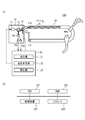
- (A) is the schematic showing the whole structure of the temperature measuring device which concerns on embodiment
- (b) is a block diagram for demonstrating the hardware constitutions of a control part. It is a figure showing the component of backscattered light.
- (A) is a figure which illustrates the relationship between the elapsed time after light-pulse emission by a laser, and the light intensity of a Stokes component and an anti-Stokes component
- (b) shows the detection result of (a), and Formula (1). It is the temperature calculated using.
- Detailed procedure of double-end method Represents the advantages of the double-ended method. An example of response when a part of the optical fiber is immersed in hot water of about 55 ° C. at room temperature of about 24 ° C. is shown.
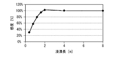
- FIG. 6 It is a figure which illustrates the result obtained from FIG. 6 and Formula (3).
- the typical example of an impulse response is illustrated.
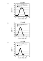
- (A)-(c) is a figure which illustrates a comparison with the output waveform estimated from the impulse response with respect to each immersion length, and the output waveform actually obtained.
- For the two 20 cm high temperature application sections a section not applied at the center is provided, and the calculated value of the output waveform when the width of the section is gradually changed is illustrated.
- An example of the temperature distribution when a pulse is incident from one end obtained by backward Raman scattered light detection is shown.
- FIG. 12 is a diagram in which temperatures are calculated by averaging Stokes components and anti-Stokes components of two signals incident from both ends of FIG. 11. The measurement accuracy is exemplified quantitatively.
- FIG. 10 is a diagram illustrating a Stokes component and an anti-Stokes component, which are original signals for calculating the temperature distribution illustrated in FIGS. 9A to 9C.
- (A) to (c) are other data in which a section different from FIG. 16 is immersed in hot water when a light pulse is incident from the first end.
- FIG. 17 is an enlarged view of 4800 m to 5100 m in FIG.
- FIG. 17 is an enlarged view of 4800 m to 5100 m in FIG.
- FIG. 17 is a diagram illustrating a comparison of Pearson's product moment correlation coefficient and Spearman's rank correlation coefficient with respect to the data of FIG. 16. It is another example of the flowchart performed when a correction
- (A) And (b) is a figure which illustrates another example of application. It is a figure which illustrates another example of application.
- (A)-(d) is a figure which illustrates a calculation result. It is a figure which shows the relationship between the number of one side average elements of 01A and 02A. It is a figure which shows the relationship between the number of one side average elements of 01A and 02A. It is a figure which illustrates the temperature calculation result of a double end system. It is a figure which illustrates the temperature calculation result of a double end system. It is a figure which shows the quantitative comparison of the temperature distribution before and behind a process.
- (A)-(d) is a figure which illustrates a calculation result.
- FIG. 1A is a schematic diagram illustrating an overall configuration of a temperature measuring apparatus 100 according to the embodiment.
- the temperature measuring device 100 includes a measuring machine 10, a control unit 20, and the like.
- the temperature measuring device 100 is connected to the optical fiber 30.
- the measuring device 10 includes a laser 11, a beam splitter 12, an optical switch 13, a filter 14, a plurality of detectors 15a and 15b, and the like.
- the control unit 20 includes an instruction unit 21, a temperature measurement unit 22, a correction unit 23, and the like.
- FIG. 1B is a block diagram for explaining the hardware configuration of the control unit 20.
- the control unit 20 includes a CPU 101, a RAM 102, a storage device 103, an interface 104, and the like. Each of these devices is connected by a bus or the like.
- a CPU (Central Processing Unit) 101 is a central processing unit.
- the CPU 101 includes one or more cores.
- a RAM (Random Access Memory) 102 is a volatile memory that temporarily stores programs executed by the CPU 101, data processed by the CPU 101, and the like.
- the storage device 103 is a nonvolatile storage device.
- the storage device 103 for example, a ROM (Read Only Memory), a solid state drive (SSD) such as a flash memory, a hard disk driven by a hard disk drive, or the like can be used.
- a ROM Read Only Memory
- SSD solid state drive
- the CPU 101 executes the temperature measurement program stored in the storage device 103
- an instruction unit 21, a temperature measurement unit 22, a correction unit 23, and the like are realized in the control unit 20.
- the instruction unit 21, the temperature measurement unit 22, and the correction unit 23 may be hardware such as a dedicated circuit.
- the laser 11 is a light source such as a semiconductor laser, and emits laser light in a predetermined wavelength range in accordance with an instruction from the instruction unit 21.
- the laser 11 emits light pulses (laser pulses) at predetermined time intervals.
- the beam splitter 12 makes the optical pulse emitted from the laser 11 enter the optical switch 13.
- the optical switch 13 is a switch for switching the emission destination of the incident optical pulse, and injects the optical pulse alternately into the first end and the second end of the optical fiber 30 at a constant period in accordance with an instruction from the instruction unit 21.
- the length of the optical fiber 30 is L meters (m)
- the position of the first end is 0 meters (m)
- the position of the second end is L meters (m).
- the light pulse incident on the optical fiber 30 propagates through the optical fiber 30.
- the light pulse gradually attenuates and propagates through the optical fiber 30 while generating forward scattered light traveling in the propagation direction and back scattered light (returned light) traveling in the feedback direction.
- the backscattered light passes through the optical switch 13 and enters the beam splitter 12 again.
- the backscattered light incident on the beam splitter 12 is emitted to the filter 14.
- the filter 14 is a WDM coupler or the like, and extracts a long wavelength component (a Stokes component described later) and a short wavelength component (an anti-Stokes component described later) from the backscattered light.
- the detectors 15a and 15b are light receiving elements.
- the detector 15a converts the received light intensity of the short wavelength component of the backscattered light into an electrical signal and transmits it to the temperature measurement unit 22 and the correction unit 23.
- the detector 15 b converts the received light intensity of the long wavelength component of the backscattered light into an electrical signal and transmits it to the temperature measurement unit 22 and the correction unit 23.
- the correction unit 23 corrects the anti-Stokes component.
- the temperature measurement unit 22 performs temperature measurement using the Stokes component and the anti-Stokes component.
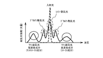
- FIG. 2 is a diagram showing components of backscattered light.
- backscattered light is roughly classified into three types. These three types of light are in order of increasing light intensity and closer to the incident light wavelength, such as Rayleigh scattered light used for OTDR (optical pulse tester), Brillouin scattered light used for strain measurement, temperature measurement, etc.
- Raman scattered light used in The Raman scattered light is generated by the interference between the lattice vibration in the optical fiber 30 that changes according to the temperature and the light. Short-wavelength components called anti-Stokes components are generated by the strengthening interference, and long-wavelength components called Stokes components are generated by the weakening interference.
- FIG. 3A is a diagram illustrating the relationship between the elapsed time after light pulse emission by the laser 11 and the light intensity of the Stokes component (long wavelength component) and the anti-Stokes component (short wavelength component).
- the elapsed time corresponds to the propagation distance in the optical fiber 30 (position in the optical fiber 30).
- the light intensities of the Stokes component and the anti-Stokes component both decrease with elapsed time. This is because the light pulse gradually attenuates and propagates through the optical fiber 30 while generating forward scattered light and back scattered light.
- the light intensity of the anti-Stokes component is stronger than the Stokes component at a position where the temperature is high in the optical fiber 30, and compared to the Stokes component at a position where the temperature is low. Become weaker. Therefore, the temperature at each position in the optical fiber 30 can be detected by detecting both components with the detectors 15a and 15b and using the difference in characteristics between the two components.
- the region showing the maximum is a region where the optical fiber 30 is intentionally heated with a dryer or the like in FIG.
- region which shows minimum is an area
- the temperature measurement unit 22 measures the temperature from the Stokes component and the anti-Stokes component for each elapsed time. Thereby, the temperature of each position in the optical fiber 30 can be measured.
- the temperature measurement unit 22 measures the temperature at each position in the optical fiber 30 by calculating the temperature according to the following formula (1), for example.
- FIG. 3B shows the temperature calculated using the detection result of FIG. 3A and the above equation (1).
- the horizontal axis of FIG.3 (b) is the position in the optical fiber 30 calculated based on elapsed time.
- the temperature at each position in the optical fiber 30 can be measured by detecting the Stokes component and the anti-Stokes component.
- the laser 11 makes an optical pulse incident on the optical fiber 30 at a constant period.
- the spatial resolution is improved as the pulse width of the light pulse is narrowed.
- the temperature can be measured by the above equation (1).
- the incident position is alternately switched between the first end and the second end at a constant cycle as in the present embodiment, the anti-Stokes light amount and the Stokes light amount are averaged at the position of each optical fiber 30 (calculation of the average value). )do it.
- This switching method is called “loop measurement”, “double end measurement”, “dual end measurement”, or the like (hereinafter referred to as a double end method).
- the above formula (1) may be changed to the following formula (2).
- the anti-Stokes light amount and the Stokes light amount may be averaged at each position of the optical fiber 30 in the above formula (1).
- the offset and gain can be set by using an average value or a larger value at the time of measurement at the end, or by newly calibrating.
- Temperature Gain / ⁇ Offset-2 ⁇ ln (Average anti-Stokes light quantity / Average Stokes light quantity ⁇ (2)
- Fig. 4 shows the detailed procedure of the double-ended method.
- “01S” indicates a Stokes component when an optical pulse is incident from the first end (0 ⁇ L).
- “01A” indicates an anti-Stokes component when an optical pulse is incident from the first end (0 ⁇ L).
- “02S” indicates a Stokes component when an optical pulse is incident from the second end (L ⁇ 0).
- “02A” indicates an anti-Stokes component when an optical pulse is incident from the second end (L ⁇ 0).
- “02S” and “02A” can be obtained by inverting the light intensity “02S ′” and “02A ′” detected when the light pulse is incident from the second end with respect to the elapsed time. it can. The position can be unified by this inversion.
- Fig. 5 shows the advantages of the double-ended method. If excessive bending occurs in the path, transmission loss occurs, and the light intensity sharply decreases at that point. When the light intensity sharply decreases, the ratio between the Stokes component and the anti-Stokes component changes, and the temperature calculated by the above equation (2) usually shifts in the decreasing direction.
- the end-end method that is not a double-end method (hereinafter referred to as a single-end method)
- the bending loss point to the second end On the side the output temperature for the same applied temperature decreases.
- the pulse propagates from the second end (L meter) side to the first end (0 meter) side
- the output temperature with respect to the same applied temperature decreases from the bending loss point to the first end side.
- the temperature of the first end or the second end can be calibrated using a resistance temperature detector for calibration.
- a resistance temperature detector for calibration.
- difference of a value may arise far from the calibrated location.
- the double end method the following merits can be obtained by taking an average. (1) The steep change before and after the bending loss point can be canceled, that is, the change in the length direction of the loss can be eliminated. (2) Since each starting temperature calibrated with a single-ended type resistance temperature detector and the temperature at the same position in the double-ended type should not change, the gain and offset value can be recalibrated to do so.
- the optical fiber currently distributed does not have a non-uniform refractive index due to improved performance, transmission loss of different sizes may occur due to bending, tension, connector connection, etc. when laying on each target. Therefore, in order to accurately measure the temperature in the single-ended method, it is preferable to assign a unique calibration value to the section after each loss occurs. However, it is not possible to compensate for the loss that occurred during the measurement, but in the double-ended method, the occurrence of transmission loss affects the length of use, which is not desirable, but you do not have to worry about whether or not accurate measurement is possible. Good.
- FIG. 6 shows a response example when a part of the optical fiber 30 is immersed in hot water of about 55 ° C. at a room temperature of about 24 ° C.
- the peak temperature is 55 ° C. which is the same as that of hot water at about 2 m or more. Therefore, in order to measure an accurate temperature, it is preferable to lengthen the temperature measurement target section.
- the sensitivity of the measurement system is defined by the following equation (3).
- Sensitivity (peak temperature at hot water immersion position-room temperature measured with fiber before and after immersion position) / applied temperature x 100 (%) (3)
- FIG. 7 a slight overshoot is observed. This is because the impulse response of the system is not Gaussian and has a negative component close to a sinc function and a higher-order peak, as will be described later.
- the minimum length at which the sensitivity is 100% or can be considered is referred to as the minimum heating length.
- the impulse response of the system is obtained.
- FIG. 8 illustrates a typical example of the determined impulse response.
- the impulse response can be regarded as a waveform that has been subjected to window function processing such that a position away from the center is attenuated cleanly in a sinc function.
- the overshoot of the sensitivity curve in FIG. 7 is caused by this impulse response waveform. If this impulse response is convoluted with the applied temperature distribution along the length direction of the optical fiber 30, the output can be predicted almost accurately.
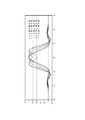
- FIGS. 9A to 9C are diagrams illustrating a comparison between an output waveform estimated from an impulse response for each immersion length and an actually obtained output waveform. As illustrated in FIGS. 9A to 9C, the output waveform can be predicted almost accurately. In the 3.25 m immersion of FIG. 9A, the peak is flattened due to interference between impulse response convolutions.
- FIG. 10 a section not applied to the center is provided for the two high temperature application sections of 20 cm (that is, in the case of immersion in hot water, it is taken out into the air), and the width of the section is gradually changed.
- the minimum temperature in the central non-heating section becomes equal to the reference temperature, that is, the interference of the impulse response waveform can be ignored. This is a case where the width is larger than the interval width, for example, about the primary component width.
- the zeroth-order component width is centered on that position. It is preferable to pay attention to the temperature change in the above-described range and the primary component width or less.
- the light pulse propagates while gradually spreading and attenuating due to the influence of wavelength spread, incident angle of view, scattering, and the like. Therefore, it is preferable that the impulse response is measured and calculated at the center position when the fiber having the maximum usable length described in the specification of the optical fiber 30 is connected, or the impulse response is measured at the near end, the center, or the far end. It is preferable to take measures such as taking the average of the places.
- a plurality of ranges in which the difference between the convolution and the output data as illustrated in FIGS. are preferably measured, calculated and stored at the center position of each section, and the stored impulse response is used for each section. Since the impulse response waveform changes slightly with the passage of time due to laser degradation or the like, it is preferable to calibrate the impulse response at the same position as the first acquisition for every predetermined period in order to measure temperature with higher accuracy. .
- FIG. 11 shows an example of a temperature distribution when a pulse is incident from one end obtained by detection of backward Raman scattered light.
- the waveform when entering from the first end (0 meter) illustrated in FIG. 1 and the waveform when entering from the second end (L meter) are illustrated in an overlapping manner.
- the variation in the measured temperature is small near the first end, and the variation in the measured temperature increases toward the second end.
- the variation in measured temperature is small near the second end, and the variation in measured temperature increases toward the first end.
- the vicinity of 3000 m where the temperature change is large is a connector connection position where cleaning is insufficient, and the 4900 m point is a place immersed in hot water.
- the optical fiber 30 is wound around a plurality of bobbins to form a path, and since the average temperatures thereof are slightly different, a plurality of steps are generated. As can be seen from FIG. 11, the further away from the light source, the larger the variation and the lower the measurement accuracy.
- FIG. 12 shows the temperature obtained by averaging (calculating an average value) the Stokes component and the anti-Stokes component of the two signals incident from both ends of FIG.
- the averaging calculates an average value
- the Stokes component and the anti-Stokes component of the two signals incident from both ends of FIG. By the averaging, the decrease in the measurement accuracy of the end point is moderated as compared with FIG. 11, but does not reach the end point on the good side.
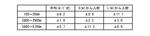
- FIG. 13 quantitatively illustrates the measurement accuracy. This is the value of the standard deviation 3 ⁇ calculated using the values of 100 m for each of the three flat portions where there is no temperature change. It can be confirmed that the average (loop type) is an average value of the value when incident from 0 (m) and the value when incident from L (m).
- a bandpass filter that cuts both low and high frequencies (and midrange) other than the required signal band, and a noise model are designed, and an effective signal band is determined based on it.
- applications such as adaptive filters to extract.
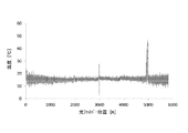
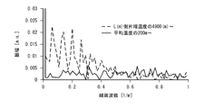
- FIG. 14 the temperature distribution of the immersion section of the L meter side one end with less noise extracted from FIG. 11 and the flat temperature portion near 200 m extracted from FIG. 12 are illustrated. The fluctuation of the temperature of the flat temperature part is due to noise.
- the measurement of the double end method is performed, as described above, in addition to the problem that the measurement accuracy of the end near the light source is poor compared to the vicinity of the center. There is a problem in that attenuation of the signal component itself is unavoidable even if some filtering process is added for relaxation.
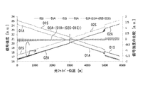
- FIG. 16 illustrates Stokes components and anti-Stokes components, which are original signals for calculating the temperature distribution illustrated in FIGS. 9A to 9C.
- the Stokes component “01S” and the anti-Stokes component “01A” when the light pulse is incident on the first end the Stokes component “02S” and the anti-Stokes component “01” when the light pulse is incident on the second end.
- 02A "is exemplified.
- the following formula (4) is illustrated on the second axis. 02A- (01A + (02S-01S)) (4)
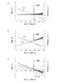
- FIGS. 17 (a) to 17 (c) are other data in which a section different from that in FIG. 16 is immersed in hot water when a light pulse is incident from the first end (0 ⁇ L). While FIG. 17A shows an appropriate temperature distribution, the difference between FIG. 17B and FIG. 17C is whether the temperature continues to increase or decreases as the far end is reached. Has occurred. The amount of attenuation in the length direction of the anti-Stokes component is changed so as to be small in FIG. 17B and large in FIG. Regardless of the single-ended method or double-ended method, the output temperature distribution must be substantially the same except for noise components. Therefore, the correction of the loss of the anti-Stokes component is adjusted so as to have a distribution as shown in FIG. In this case, the attenuation values in the length direction of the Stokes component and the anti-Stokes component are substantially equal.
- FIGS. 17A to 17C is a case where an optical pulse is incident from the first end (0 ⁇ L), but even when an optical pulse is incident from the second end (L ⁇ 0). The same can be said. Therefore, since the total attenuation from the incident end to the exit end is the same for both the incident from the 0 (m) side and the incident from the L (m) side, the equation (4) in FIG. It can be seen that it is probable that the value is almost zero.
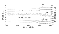
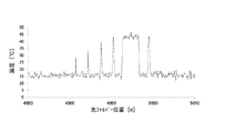
- FIG. 18 (a) and 18 (b) show enlarged views of 4800m to 5100m in FIG. FIG. 18B is different from FIG. 16 and illustrates the measured temperature obtained using the following equation (5).
- the signal intensity is lower when the light pulse is incident from the first end side, and the noise is reduced.
- FIG. 18 (a) and FIG. 18 (b) it appears that it is changing with a certain variation regardless of the influence of the temperature change. Accordingly, it can be said that 01A can be estimated to a certain extent using the other three components together with the estimation from FIGS. 17 (a) to 17 (c).
- FIG. 19 attention is now focused on the Stokes component (01S in FIG. 18A) and the anti-Stokes component (01A in FIG. 18A) when the pulse is incident from the first end (0 ⁇ L).
- the value of Pearson's product-moment correlation coefficient is shown in a data range of ⁇ 2 m centering on the current position.
- 01A considering 01A as a reference, if at least one pair of three signals 01S, 02A, and 02S has a high correlation, it is considered that a significant temperature change has occurred. It is done. That is, when the correlation is low, it is considered that the temperature does not change or is changing slowly, so that even if estimation using the above three components is performed, there is no difference in output.
- the noise component is the next largest.
- the change in temperature means that the Stokes component and the anti-Stokes component change in synchronization with the length direction of the optical fiber 30.
- the synchronization range can be limited, it can be considered that the other regions do not change with respect to the temperature of the adjacent fiber position on the light source side, or that the inclination changes gently.
- Optical fiber temperature measurement by detection of back Raman scattered light may show approximately the same minimum heating length response within a certain interval.
- the fiber having the minimum heating length is heated more than around the constant temperature, a waveform almost the same as the impulse response of FIG. 6 is obtained.
- the range interference range
- the range that affects the surroundings within the range of the 0th-order component width where the gradient is reversed and the 1st-order component width where the amplitude is attenuated to almost zero.
- the maximum averaging range is set as “a range of the zeroth-order component width or more and the first-order component width or less in which the amplitude is attenuated to substantially zero”, and the number of averaging elements corresponding to the magnitude of the correlation ( Noise is reduced by determining an averaging range) and replacing the averaged position with a value averaged around the currently focused position in accordance with the number of averaged elements. Further, when an optical pulse is incident from the 0 meter (first end) side, the vicinity of the L meter (second end) is the far end.
- FIG. 20 is an example of a flowchart executed when the temperature measuring device 100 measures the temperature.
- the optical fiber 30 is used.
- the temperature measuring apparatus 100 executes the flowchart of FIG. 20 for each of the three sections.
- the correction unit 23 determines whether or not the section of the focused optical fiber is the first section that is 1/3 or less of the total length of the optical fiber 30 (step S1). When it is determined as “Yes” in step S1, the correction unit 23 sets the predetermined range set to be not less than the zeroth-order component width and not more than the first-order component width of the minimum heating length response waveform with each sample point in the first section as the center. The magnitude of the correlation (specified range) is obtained for each sample point. The sample point is a temperature measurement target point in the length direction of the optical fiber 30. First, the correction unit 23 obtains a correlation coefficient between 02S and 01S and a correlation coefficient between 02S and 01A at each sample point, and holds the smaller correlation coefficient as ⁇ — 02S (step S2). Next, the correction unit 23 obtains the correlation coefficient between 02A and 01S and the correlation coefficient between 02A and 01A at each sample point, and holds the smaller correlation coefficient as ⁇ — 02A (step S3).
- Pearson's product moment correlation coefficient can be used.
- the Pearson product moment correlation coefficient in the case of 02A and 01S is expressed by the following equation (6).
- Correlation coefficient ⁇ (covariance of 02A in the same range as 01S in the specified range) / (standard deviation of 01S in the same range) / (standard deviation of 02A in the same range) (6)
- the Pearson product moment correlation coefficient centered on the sample point k of the optical fiber 30 is ⁇ [k]
- the 01S array is 01S [k]
- the 02A array is 02A [k]
- the number of samples in the specified range is n
- the above formula (6) can be specifically expressed as the following formula (7).
- the modified Spearman rank correlation coefficient when using the modified Spearman rank correlation coefficient, first, in the specified range (n in the above formula (7)), 01S and 02A are ranked among the n. Pearson's product moment correlation coefficient is used for the ranks. When there is the same rank, the correction formula is used. Usually, the Stokes component and the anti-Stokes component hardly occur at the same rank, and therefore, the process of making the first occurrence higher may be used.
- ⁇ 3.6 m is set as a range that matches the above condition, and comparison of Pearson's product-moment correlation coefficient and Spearman's rank correlation coefficient with respect to the data in FIG. Is illustrated in FIG.
- the Pearson product moment correlation coefficient is 1 or ⁇ 1
- a perfect correlation a high correlation of 0.7 to less than 1 in absolute value
- a correlation of 0.4 to less than 0.7, 2 to less than 0.4 is treated as low correlation
- 0.2 or less is treated as no correlation.
- the slope of Spearman changes more in the region of 0.2 or less where there is no correlation, it is almost 1: 1 for the value of 0.3 or more in the low correlation range. Produces equivalent results. If it is standardized, it may be made by itself or of course using other correlation coefficients.
- the correction unit 23 determines whether or not the correlation coefficient ⁇ — 02A is equal to or less than a predetermined value (for example, 0.2 or less) at each sample point (step S4). When it is determined as “Yes” in step S4, the correction unit 23 replaces 02A with the alternative 02A at the sample point (step S5).
- a predetermined value for example, 0.2 or less
- the alternative 02A can be represented by the following formula (8).
- Alternative 02A 01A + (AVERAGE1 (02S) ⁇ 01S) + (AVERAGE2 (02A) ⁇ AVERAGE2 (01A)) ⁇ (AVERAGE2 (02S) ⁇ AVERAGE2 (01S)) (8)
- AVERAGE1 is an average whose interval is variable according to the signal quality of the sample point of interest.
- AVERAGE2 is an average of fixed widths centered on the sample point currently focused on.
- the correction unit 23 determines the averaging range of AVERAGE 1 according to the small correlation coefficient between 02S and 01S and the small correlation coefficient between 02S and 01A.
- an integer sample obtained by rounding 1 / ⁇ — 02S may be used as the average range of AVERAGE1.
- the average range of AVERAGE 1 becomes larger as the correlation coefficient of the position currently focused on is smaller.
- the upper limit value of the averaging range of AVERAGE 1 is preferably in the range of the zeroth-order component width or more and the first-order component width in which the amplitude is attenuated to almost zero as described above.
- the alternative 02A uses the second term with AVERAGE1 (02S) as 02S in the formula “02A ⁇ (01A + (02S-01S)” used to describe the second axis in FIG.
- the slight offset value AVERAGE2 (02A)-(AVERAGE2 (01A)-(AVERAGE2 (02S) -AVERAGE2 (01S))) in item 2 is subtracted.
- the average range is larger than the average range of AVERAGE 1 at the center.
- step S5 After the execution of step S5 or when determined “No” in step S4, the temperature measurement unit 22 uses the average value of 01S and 02S as the average Stokes component and the average value of 01A and 02A as the anti-Stokes component. Then, the temperature is measured using the above formula (2) (step S6). That is, if “Yes” is determined in step S4, the temperature is calculated after 02A is replaced with alternative 02A, and if “No” is determined in step S4, 02A is replaced with alternative 02A. Without calculating the temperature.
- the reliability value is relatively weighted with less noise, and noise can be removed.
- the larger one may be used and an average may be used. The smaller one means that the data other than the one that seems to be a temperature change is averaged, and the larger one means that the slight change data buried in the noise is not removed as much as possible. That's it.
- the correction unit 23 determines whether or not the section of the optical fiber of interest is a third section that is 2/3 or more of the total length of the optical fiber 30 (Step S ⁇ b> 1). S7).
- 02S corresponds to 01S
- 02A corresponds to 01A. Therefore, if “Yes” is determined in Step S7, the correction unit 23 replaces 02S and 01S, replaces 02A and 01A, and performs the same processing as Steps S2 to S6 (Step S8). Therefore, when the correlation coefficient ⁇ _01A is a predetermined value (for example, 0.2 or less), 01A is replaced with an alternative 01A of the following formula (9).
- the first term and the second term on the right side use the above-mentioned three signals, and the third term is a correction term for the slightly generated offset.
- the slight offset term is not exactly divided into the correction of the attenuation amount of the anti-Stokes component with respect to the Stokes component in the case of the single-end method described with reference to FIGS. This is the same when a light pulse is incident from the opposite L meter (second end) side. Therefore, the offset component is removed using a wide averaging range AVERAGE2.
- the alternative 01A Is obtained by subtracting this component, and the same can be said for the alternative 02A in the first section described above, where the alternative 01A is expressed by the following formula (10). Is equal to equation (9).
- Alternative 01A 02A + (AVERAGE1 (01S) ⁇ 02S) + (AVERAGE2 (02S) ⁇ AVERAGE2 (01S)) ⁇ (AVERAGE2 (02A) ⁇ AVERAGE2 (01A)) (10)
- the temperature measurement unit 22 sets the average value of 01S and 02S as an average Stokes component, and sets the average value of 01A and 02A as an anti-Stokes component, and the above equation (2). Using this, the temperature is measured (step S9).
- the reciprocal of the magnitude of the correlation coefficient is used as an index of the averaging range, but the reciprocal may not necessarily be used.
- the averaging range may be relatively narrowed as the correlation coefficient is large, and the averaging range may be relatively large as the correlation coefficient is small.
- the averaging range of AVERAGE 1 may be a fixed interval regardless of the signal quality of the sample points.
- the procedure for determining whether to replace 02A with the alternative 02A using ⁇ _02A in step S4 the procedure for determining whether to replace 01A with the alternative 01A using ⁇ _01A in step S8 are exactly the same, and AVERAGE2 It is also the same that the averaging range of is larger than the averaging range of AVERAGE1.
- FIG. 22 is another example of a flowchart executed when the temperature measuring unit 100 measures the temperature.
- FIG. 22 is different from FIG. 20 in that, when “No” is determined in step S4, the averaging ranges of 02S and 02A are each an integer sample rounded to 1 / ⁇ — 02S on one side and averaged. This is a point to be replaced with a value (step S10).
- step S10 step S6 is executed.
- FIG. 23 is another example of a flowchart executed when the temperature measuring apparatus 100 measures the temperature.
- the difference between FIG. 23 and FIG. 22 will be described.
- the optical fiber 30 is divided into a first section, a third section in the center, and an L meter (second end) where the measurement precision near 0 meter (first end) is poor.
- the correction unit 23 executes the flowchart of FIG. 23 for each of the five sections.
- the correcting unit 23 determines whether or not the section of the focused optical fiber is the first section that is 1/5 or less of the total length of the optical fiber 30 (step S11). If it is determined as “Yes” in step S11, the correction unit 23 executes steps S12 to S14 of the same processing as steps S2 to S4.
- the predetermined value used in step S14 is referred to as a first threshold value.
- amendment part 23 performs step S15 of the process similar to step S5.
- step S14 determines whether or not the correlation coefficient ⁇ — 02A is equal to or larger than a second threshold value (for example, 0.55) larger than the value 1 used in step S14. (Step S16). If it is determined as “Yes” in step S16 or after execution of step S15, step S17 of the same process as step S6 is executed. If “No” is determined in step S16, step S18 of the same process as step S10 is executed. After execution of step S18, step S17 is executed. In S16, even if ⁇ _02A is equal to or greater than the second threshold value, ⁇ _02S may be a small value. In this case, similarly to S18, the averaged range on one side may be replaced with a value averaged as an integer part rounded to 1 / ⁇ — 02S.
- a second threshold value for example, 0.55
- the correcting unit 23 determines whether or not the section of the optical fiber of interest is 4/5 or more of the total length of the optical fiber 30 (Step S19). If “Yes” is determined in step S19, the same processing as in steps S12 to S18 is executed after the procedure of replacing 02S and 01S and replacing 02A and 01A in steps S12 to S18 ( Step S20).
- step S21 determines whether or not the section of interest is 2/5 or less of the total length of the optical fiber 30 or 3/5 or more. Determination is made (step S21). If “Yes” in step S21 and 2/5 or less of the total length, the same processing as in steps S12 to S18 is executed. However, different values are used as the threshold for the correlation coefficient and the averaging upper limit. If “Yes” in step S21 and 3/5 or more of the total length, the same processing as in step S20 is executed. However, different values are used as the threshold for the correlation coefficient and the averaging upper limit. Thereby, the correction
- the averaging range is set to be equal to or smaller than the primary component width of the minimum heating length. This is due to the possibility that the averaged signal is greatly affected by the crosstalk of adjacent signals beyond that.
- the obtained correlation coefficient is ⁇ 1
- it is usually classified as perfect correlation, but in the present application, it is treated as noise. This is because, for example, when the temperature rises, both Stokes and anti-Stokes protrude upward, and when the temperature decreases, both protrude downward. In this case, the anti-Stokes will not have a shape that inverts the Stokes component upside down. In such a case, it is usually a noise state or a poorly connected connector or a fiber with a large refractive index difference. This is because it is only for fusion or connector connection.
- the division is set to 3 or 5.
- two divisions divided at the center four divisions obtained by further halving each division, and eight divisions that are half of the division may be used.
- 01S, 01A, 02S, and 02A all have no central section in which the temperature is calculated without any processing.
- the correlation coefficient between 02A and 01S in a predetermined region including sample points of a partial region on the first end side When at least one of the correlation coefficients between 02A and 01A is equal to or less than the threshold value, 02A is replaced with an alternative value corresponding to 01S, 01A, and 02S. In this case, when noise appears large in 02A, 02A is replaced with a value corresponding to 01S, 01A, and 02S with less noise. Thereby, noise of 02A can be reduced.
- 01S and 01A are components immediately before 02A with respect to the switch by the optical switch 13.
- the components are not limited to just before and may be components before 02A.
- the component after 02A may be sufficient.
- 02S and 02A are preferably components immediately before 01A with respect to the switch by the optical switch 13, but are not limited to just before and may be components before 01A.
- the component after 01A may be sufficient.
- the condition for replacement of 02A may be whether or not at least one of 02A and 01A, 02S and 01S, 02S and 01A is equal to or less than a threshold.
- the replacement condition for 01A may be, for example, whether or not at least one of 01S and 02A, 01A and 02A, 01S and 02S, 01S and 02A is equal to or less than a threshold value.
- the average value of the Stokes component and the anti-Stokes component is obtained in the averaging range, but it is only necessary to suppress the variation in data in the range. Therefore, other averages such as an arithmetic average considering weighting, a geometric average, and a harmonic average may be used. In addition, when obtaining an average value of 01S and 02S and an average value of 01A and 02A, an arithmetic average considering weighting may be used.
- the temperature measurement apparatus 100 can be applied to various temperature measurement objects.
- FIG. 24 it is conceivable to lay an optical fiber in a branch pipe of a high-temperature and high-pressure raw material transport pipe.
- heat insulation and protection are provided by the racking material and the outer metal plate, so even if leakage occurs due to corrosion of the connection joint, it does not lead to a serious situation that leads to fire accidents, etc. Often not found. Therefore, it is wrapped around the connection joint of the optical fiber, and by comparing the correlation between changes in the temperature at each optical fiber position, even if the outside air temperature or the internal temperature / pressure changes, the leakage of the connection can be accurately performed.
- Presence or absence can be detected early.
- a means for comparing the correlation between the temperatures of the respective optical fiber positions there is a method of generating a dispersion covariance matrix using the temperature of each optical fiber position as an element and performing an outlier test by a method such as Mahalanobis distance or MSD method.
- FIG. 25 exemplifies application to a method of measuring the passing air temperature by a number of winding parts manufactured with a single optical fiber. Each wound portion is wound around the same place several times with substantially the same diameter and is connected to the adjacent wound portion. What temperature distribution should be obtained if the average temperature of each winding unit is acquired using the measuring device 10 and the control unit 20 according to the above embodiment and gradation is generated as the representative temperature of the center position coordinates of each winding unit? It is possible to measure whether or not the wind passes through the sheet / frame where the fiber is laid. As the number of turns wound around each winding part is increased, the number of measurement points to be averaged is increased and the apparent measurement accuracy is improved, so that a desired measurement accuracy can be obtained in a short time measurement.
- the attenuation of the incident pulse is reduced, so that the measurement accuracy is improved.
- the output temperature data itself is required to be highly accurate. If the above embodiment is applied, this requirement can be realized.
- FIGS. 26 (a) and 26 (b) exemplify an example in which a fiber net in which a large number of winding parts manufactured using heat-resistant fibers are connected is laid on the surface of the melting furnace. Each fiber net is connected, but the fiber at the inlet end and the outlet end of the two nets at the end is connected to the measuring machine 10 and the control unit 20 to perform a double-end measurement.
- the relationship between the positions of the nets 1 to 3 and the temperature distribution is displayed in the two-dimensional gradation shown in FIG. 26B, and the generated two-dimensional gradation is generated at a position corresponding to the direction of each net with respect to the reference direction of the melting furnace. By fitting, the surface temperature of the melting furnace can be visualized easily.
- the Mahalanobis distance is calculated using the time transition of the relative relationship between the temperature changes of the winding portions of each net, as in the application example of FIG. Even in the case of analyzing a sign of abnormality from a change or a change in a value calculated by the MSD method, temperature measurement can be performed with high accuracy.
- FIGS. 27 (a) and 27 (b) illustrate application to a system that performs air conditioning management using optical fibers laid in a straight line above the server rack in the data center.
- installation may not be permitted for server racks. Therefore, as illustrated in FIGS. 27A and 27B, the optical fiber is laid in a straight line or a certain amount of meandering to the exhaust surface side, etc., on the intake surface of the server rack. Then, the temperature of the rack part is measured in advance by some method, and the length of the optical fiber corresponding to the upper part of each rack is determined by associating the number of margins with the installed optical fiber. Set the alarm threshold.
- the server rack is generally about 60 cm or 70 cm.
- the number of measurement points is only one or two points. is required.
- temperature measurement can be performed with high accuracy.
- control that can increase the margin by increasing the air conditioning becomes possible, and both energy saving and safety can be achieved.
- FIG. 28 illustrates the application to the cultivation of high-quality fruits and theft prevention in a greenhouse.
- the example of FIG. 28 is based on the premise of cultivation of crown melon, for example.
- An optical fiber for measuring soil temperature, ambient temperature, fruit temperature, etc. is installed, and an optical fiber for humidity management using the same principle as a moisture meter is installed, and temperature and temperature are measured using Raman scattering. Humidity can be measured.
- the measurement accuracy of the system is required to be good.
- the time value transition of each temperature is managed in detail and integrated value management is performed to perform good growth, it is required that the measurement accuracy of the system is also good. This requirement can be realized by using the above embodiment.
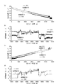
- FIG. 29A shows a comparison between 01S and 01A before and after processing.
- FIG. 29A although variation was observed on the far end side before the processing, the variation was suppressed after the processing.
- FIG. 29 (b) is an enlarged view of the vicinity of a region immersed in hot water.
- FIG. 29B especially for the anti-Stokes component, the variation before the processing was greatly suppressed after the processing.
- FIG. 29 (c) is a comparison before and after processing for 02S and 02A.
- FIG. 29C although variation was observed in the vicinity of 0 (m) which is the far end, the variation was suppressed after processing.
- FIG. 29 (d) is an enlargement of a region immersed in hot water. As illustrated in FIG. 29 (d), it is slightly improved as compared with FIG. 29 (b), but it is almost no processing. This is because the noise component is small because of the near end.
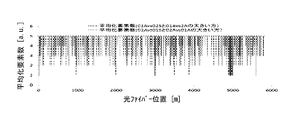
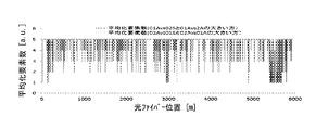
- FIG. 30 and 31 show the relationship between the number of one-side average elements of 01A and 02A determined based on the processing of FIGS. 22 and 23.
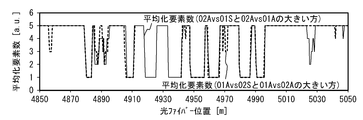
- FIG. 31 is a partially enlarged view of FIG.
- the number of one-side average elements corresponds to 1 / ⁇ _01A and 1 / ⁇ _02A.
- the alternative 01A and the alternative 02A are used in sections of 3/5 or more and sections of less than 2/5, respectively.
- FIG. 31 is compared with FIG. 29 (a) to FIG. 29 (d), and it can be seen that when the temperature change occurs and both the Stokes component and the anti-Stokes component change, both take almost the same value.
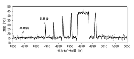
- FIGS. 32 and 33 show the double-ended temperature calculated from FIGS. 29 (a) to 29 (d), 30 and 31.
- FIG. Looking at FIG. 32 and FIG. 33 which is an enlarged view of the portion immersed in hot water, it can be seen that the noise component is suppressed without losing the temperature change component.
- the temperature in FIGS. 32 and 33 was calculated by the above equation (2). Since the number of averaging elements is 1 at a position where the correlation coefficient is 1, the temperature before and after the treatment does not change. Therefore, since the gain and the offset value used after the substitution processing need to be the same as those used before the substitution processing, they are expressed by the following formula (11).
- Processed temperature Gain / ⁇ Offset-2 ⁇ ln (Processed average anti-Stokes light quantity / Processed average Stokes light quantity) ⁇ (11)
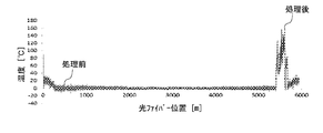
- FIG. 34 shows a quantitative comparison of the temperature distribution before and after the treatment. Since there is no change before and after the process in any case at the temperature change position, the standard deviation value 3 ⁇ at the flat portion is compared. As illustrated in FIG. 34, the value does not change in the normal temperature calculation section of 2800 m to 2900 m, but noise suppression of 83% or more is achieved in the processed section. In the case of the suppression effect of 83% obtained by the processing of the above embodiment, the measurement accuracy is 1 / 5.9. Therefore, in the case of the same measurement accuracy, the measurement time is set to 35 before the processing. , The image is compressed so that it becomes 1 after processing. Further, in the measurement by the double end method in FIG. 11, the positions of 100 m to 200 m and 5600 m to 5700 m are three times as large as the measurement accuracy of the center 2800 m to 2900 m position. In addition, the measurement accuracy on both sides is doubled.
- Example 1 A specific example of a temperature distribution obtained at a measurement object and a measurement cycle different from Example 1 will be described.
- the applied processing method is almost the same as that in the first embodiment, but the section is set to two overlapping sections of less than 3/5 of the total length and 2/5 or more. Thereby, in the overlapped section, if the magnitude of the correlation is small, all of 01A, 01S, 02A and 02S are replaced.
- FIG. 35 (a) to FIG. 35 (d) illustrate calculation results.
- FIG. 35A shows a comparison between 01S and 01A before and after processing.
- FIG. 35B is an enlarged view of the vicinity of the heating region.
- FIG. 35 (b) especially for the anti-Stokes component, the variation before the processing was greatly suppressed after the processing.
- FIG. 35 (c) is a comparison before and after the process for 02S and 02A.
- FIG. 35 (d) is an enlargement of a region immersed in hot water.
- the process is slightly improved as compared with FIG. 35B, but almost no processing. This is because the noise component is small because of the near end.
- FIG. 36 and 37 show the relationship between the number of one-side average elements of 01A and 02A determined based on the processing of FIGS. 22 and 23.
- FIG. 37 is a partially enlarged view of FIG. It corresponds to 1 / ⁇ _01A and 1 / ⁇ _02A, and when the number of averaging elements is 3 or more, the alternative 01A and the alternative 02A are used in a section of 2/5 or more and a section of less than 3/5, respectively. Yes.
- FIG. 37 is compared with FIGS. 35 (a) to 35 (d), and when the temperature change occurs and both the Stokes component and the anti-Stokes component change, both take almost the same value. However, because the change in 01S is considered noise for small temperature changes during large temperature changes, the number of averaging elements associated with 02A is somewhat larger than that associated with 01A.
- FIGS. 38 and 39 show the temperature calculated from the double-end method of FIGS. 35 (a) to 35 (d), 36 and 37.
- FIG. 40 illustrates a quantitative comparison of the temperature distribution before and after the treatment. Since there is no change before and after the process in any case at the temperature change position, the standard deviation value 3 ⁇ at the flat portion is compared. Due to the overlap, slight improvement was seen even in the middle 2800m to 2900m. In the central section, noise is superimposed on both 01A and 02A, so it is considered that there was not much improvement even if the values were replaced with each other. On the other hand, noise suppression of 86% or more is achieved in the sections on both sides. On the contrary, the accuracy of both sides is 1.5 times or more by the processing of the above embodiment.
Landscapes
- Physics & Mathematics (AREA)
- General Physics & Mathematics (AREA)
- Measuring Temperature Or Quantity Of Heat (AREA)
Abstract
Description
図1(a)は、実施形態に係る温度測定装置100の全体構成を表す概略図である。図1(a)で例示するように、温度測定装置100は、測定機10、制御部20などを備える。温度測定装置100は、光ファイバ30に接続されている。測定機10は、レーザ11、ビームスプリッタ12、光スイッチ13、フィルタ14、複数の検出器15a,15bなどを備える。制御部20は、指示部21、温度測定部22、補正部23などを備える。
温度=ゲイン/{オフセット-2×ln(アンチストークス光量/ストークス光量}} (1)
温度=ゲイン/{オフセット-2×ln(平均アンチストークス光量/平均ストークス光量}} (2)
感度=(お湯浸漬位置のピーク温度-浸漬位置前後のファイバで測定した室温)/印加温度×100(%) (3)
図6および上記式(3)から得られる結果を図7に示す。図7で例示するように、わずかにオーバーシュートが見られる。これは、後述するように、システムのインパルス応答がガウシアンではなく、sinc関数に近い負の成分および高次のピークを持つ波形のためである。感度100%となる、もしくはみなせる最小長さを最小加熱長と称する。
02A-(01A+(02S-01S)) (4)
01A-(02A+(01S-02S)) (5))
相関係数α=(指定範囲の01Sと同範囲の02Aの共分散)/(同範囲の01Sの標準偏差)/(同範囲の02Aの標準偏差) (6)

代替02A=01A+(AVERAGE1(02S)-01S)+(AVERAGE2(02A)-AVERAGE2(01A))-(AVERAGE2(02S)-AVERAGE2(01S)) (8)
AVERAGE1は、現在着目しているサンプル点の信号品質に応じて区間が可変の平均である。AVERAGE2は、現在着目しているサンプル点を中心とした固定幅の平均である。補正部23は、02Sと01Sとの相関係数の小ささ、および02Sと01Aとの相関係数の小ささに応じてAVERAGE1の平均化範囲を決める。例えば、1/α_02Sを四捨五入して得た整数サンプル分をAVERAGE1の平均化範囲としてもよい。この場合、現在着目している位置の相関係数が小さければ小さい程AVERAGE1の平均化範囲は大きくなる。ただし、AVERAGE1の平均化範囲の上限値は上記のように、0次成分幅以上かつ振幅がほぼゼロに減衰する1次成分幅以下の範囲とすることが好ましい。
代替01A=02A-(02S-AVERAGE1(01S))-(AVERAGE2(02A)-AVERAGE2(01A))+(AVERAGE2(02S)-AVERAGE2(01S)) (9)
代替01A=02A+(AVERAGE1(01S)-02S)+(AVERAGE2(02S)-AVERAGE2(01S))-(AVERAGE2(02A)-AVERAGE2(01A)) (10)
上記実施形態に係る温度測定装置100は、様々な温度測定対象に適用することができる。例えば、図24で例示するように、高温高圧の原料輸送配管の枝配管に光ファイバを敷設することが考えられる。このような高温高圧の配管では、ラッキング材および外側金属板により保温・保護がなされているため、接続継手部の腐食により漏洩が発生しても、火災事故等につながる甚大な状況にまで至らないと発見されない場合が多い。そこで、光ファイバの接続継手部に巻きつけておき、各光ファイバ位置の温度どうしの変化の相関関係を比較することで外気温や内部の温度・圧力が変化した場合でも正確に接続部の漏洩の有無を早期に検知することができる。各光ファイバ位置の温度どうしの相関関係を比較する手段として、各光ファイバ位置の温度を要素として分散共分散行列を生成し、マハラノビス距離やMSD法といった手法で外れ値検定を行う方法がある。
処理後温度=ゲイン/{オフセット-2×ln(処理後平均アンチストークス光量/処理後平均ストークス光量)} (11)
Claims (12)
- 光ファイバの第1端に光が入射する場合の後方散乱光から第1ストークス成分および第1アンチストークス成分を検出し、前記光ファイバの第2端に光が入射する場合の後方散乱光から第2ストークス成分および第2アンチストークス成分を検出する検出器と、
前記光ファイバの前記第1端側の一部の領域のサンプル点を含む所定領域において、前記第1ストークス成分および前記第1アンチストークス成分と、前記第2アンチストークス成分との相関の少なくともいずれかの大きさが閾値以下の場合に、前記第2アンチストークス成分を、前記第1ストークス成分と、前記第1アンチストークス成分と、前記第2ストークス成分とに応じた値に置き換える補正部と、
前記第1ストークス成分、前記第1アンチストークス成分、前記第2ストークス成分、および前記補正部によって置き換えられた後の前記第2アンチストークス成分を用いて前記サンプル点における温度を測定する測定部と、を備えることを特徴とする温度測定装置。 - 光源からの光を前記第1端と前記第2端とに交互に入射する光スイッチを備え、
前記補正部は、前記光スイッチから前記第1端に前記光が入射される場合の第1ストークス成分および第1アンチストークス成分と、次に前記光スイッチから前記第2端に前記光が入射される場合の第2アンチストークス成分との相関の少なくともいずれかの大きさが前記閾値以下の場合に、前記第2アンチストークス成分を、前記第1ストークス成分と、前記第1アンチストークス成分と、前記第2アンチストークス成分と同じタイミングで検出された第2ストークス成分とに応じた値に置き換えることを特徴とする請求項1記載の温度測定装置。 - 前記補正部は、前記第2アンチストークス成分を、前記第1ストークス成分と、前記第1アンチストークス成分と、前記第2ストークス成分とに応じた値に置き換える場合に、前記第2ストークス成分として、前記サンプル点を含む所定の可変範囲における前記第2ストークス成分を平滑化した値を用い、
前記可変範囲は、前記サンプル点における、前記第1ストークス成分および前記第1アンチストークス成分と、前記第2ストークス成分との相関の少なくともいずれかの大きさに応じた長さの範囲であることを特徴とする請求項1または2記載の温度測定装置。 - 前記補正部は、前記相関が小さいほど前記可変範囲を長くすることを特徴とする請求項3記載の温度測定装置。
- 前記補正部は、前記可変範囲に上限を設定することを特徴とする請求項3または4記載の温度測定装置。
- 前記補正部は、前記第2アンチストークス成分を、前記第1ストークス成分と、前記第1アンチストークス成分と、前記第2ストークス成分とに応じた値に置き換える場合に、さらに、前記サンプル点を含む所定の固定範囲における前記第1ストークス成分、前記第1アンチストークス成分、前記第2ストークス成分および前記第2アンチストークス成分を平滑化した値を用いることを特徴とする請求項1~5のいずれか一項に記載の温度測定装置。
- 前記補正部は、前記相関が閾値以上であれば、前記第2アンチストークス成分を置き換えないことを特徴とする請求項1~6のいずれか一項に記載の温度測定装置。
- 前記相関の大きさとして、Pearsonの積率相関係数を用いることを特徴とする請求項1~7のいずれか一項に記載の温度測定装置。
- 前記相関の大きさとして、Spearmanの順位積率相関係数を用いることを特徴とする請求項1~7のいずれか一項に記載の温度測定装置。
- 前記所定領域は、前記サンプル点の周囲の光ファイバを一定温度とし、前記サンプル点を中心とした最小加熱長区間に該一定温度と異なる一定の温度を付与した際に得られる温度分布の半値幅よりも大きく、1次成分幅よりも小さい領域であることを特徴とする請求項1~9のいずれか一項に記載の温度測定装置。
- 光ファイバの第1端に光が入射する場合の後方散乱光から第1ストークス成分および第1アンチストークス成分を検出し、前記光ファイバの第2端に光が入射する場合の後方散乱光から第2ストークス成分および第2アンチストークス成分を、検出器を用いて検出し、
前記光ファイバの前記第1端側の一部の領域のサンプル点を含む所定領域において、前記第1ストークス成分および前記第1アンチストークス成分と、前記第2アンチストークス成分との相関の少なくともいずれかの大きさが閾値以下の場合に、前記第2アンチストークス成分を、前記第1ストークス成分と、前記第1アンチストークス成分と、前記第2ストークス成分とに応じた値に置き換え、
前記第1ストークス成分、前記第1アンチストークス成分、前記第2ストークス成分、および置き換えられた後の前記第2アンチストークス成分を用いて前記サンプル点における温度を測定する、ことを特徴とする温度測定方法。 - コンピュータに、
光ファイバの第1端に光が入射する場合の後方散乱光から第1ストークス成分および第1アンチストークス成分を検出し、前記光ファイバの第2端に光が入射する場合の後方散乱光から第2ストークス成分および第2アンチストークス成分を検出する処理と、
前記光ファイバの前記第1端側の一部の領域のサンプル点を含む所定領域において、前記第1ストークス成分および前記第1アンチストークス成分と、前記第2アンチストークス成分との相関の少なくともいずれかの大きさが閾値以下の場合に、前記第2アンチストークス成分を、前記第1ストークス成分と、前記第1アンチストークス成分と、前記第2ストークス成分とに応じた値に置き換える処理と、
前記第1ストークス成分、前記第1アンチストークス成分、前記第2ストークス成分、および置き換えられた後の前記第2アンチストークス成分を用いて前記サンプル点における温度を測定する処理と、を実行させることを特徴とする温度測定プログラム。
Priority Applications (5)
| Application Number | Priority Date | Filing Date | Title |
|---|---|---|---|
| JP2017517556A JP6376287B2 (ja) | 2015-05-13 | 2015-05-13 | 温度測定装置、温度測定方法および温度測定プログラム |
| AU2015394728A AU2015394728B2 (en) | 2015-05-13 | 2015-05-13 | Temperature measurement device, temperature measurement method, and temperature measurement program |
| PCT/JP2015/063838 WO2016181542A1 (ja) | 2015-05-13 | 2015-05-13 | 温度測定装置、温度測定方法および温度測定プログラム |
| CN201580079711.5A CN107615028B (zh) | 2015-05-13 | 2015-05-13 | 温度测量装置、温度测量方法和存储介质 |
| US15/789,408 US10704964B2 (en) | 2015-05-13 | 2017-10-20 | Temperature measurement device, temperature measurement method, and computer-readable non-transitory medium |
Applications Claiming Priority (1)
| Application Number | Priority Date | Filing Date | Title |
|---|---|---|---|
| PCT/JP2015/063838 WO2016181542A1 (ja) | 2015-05-13 | 2015-05-13 | 温度測定装置、温度測定方法および温度測定プログラム |
Related Child Applications (1)
| Application Number | Title | Priority Date | Filing Date |
|---|---|---|---|
| US15/789,408 Continuation US10704964B2 (en) | 2015-05-13 | 2017-10-20 | Temperature measurement device, temperature measurement method, and computer-readable non-transitory medium |
Publications (1)
| Publication Number | Publication Date |
|---|---|
| WO2016181542A1 true WO2016181542A1 (ja) | 2016-11-17 |
Family
ID=57248953
Family Applications (1)
| Application Number | Title | Priority Date | Filing Date |
|---|---|---|---|
| PCT/JP2015/063838 Ceased WO2016181542A1 (ja) | 2015-05-13 | 2015-05-13 | 温度測定装置、温度測定方法および温度測定プログラム |
Country Status (5)
| Country | Link |
|---|---|
| US (1) | US10704964B2 (ja) |
| JP (1) | JP6376287B2 (ja) |
| CN (1) | CN107615028B (ja) |
| AU (1) | AU2015394728B2 (ja) |
| WO (1) | WO2016181542A1 (ja) |
Cited By (1)
| Publication number | Priority date | Publication date | Assignee | Title |
|---|---|---|---|---|
| WO2019176000A1 (ja) * | 2018-03-14 | 2019-09-19 | 富士通株式会社 | 検出装置、温度分布測定装置および検出装置の製造方法 |
Families Citing this family (5)
| Publication number | Priority date | Publication date | Assignee | Title |
|---|---|---|---|---|
| JP6561747B2 (ja) * | 2015-10-05 | 2019-08-21 | 富士通株式会社 | 温度測定装置、温度測定方法および温度測定プログラム |
| CN112747430A (zh) * | 2020-12-30 | 2021-05-04 | 深圳市利拓光电有限公司 | 基于激光设备的室内温度调控方法、装置及设备 |
| WO2023019273A1 (en) * | 2021-08-13 | 2023-02-16 | Veolia Nuclear Solutions, Inc. | Systems and methods for vitrification process control |
| CN114577367B (zh) * | 2022-05-06 | 2022-09-16 | 苏州光格科技股份有限公司 | 一种光纤温度传感器标定的方法、装置和计算机设备 |
| JP2024150208A (ja) * | 2023-04-10 | 2024-10-23 | 横河電機株式会社 | 測定装置、測定方法および測定プログラム |
Citations (3)
| Publication number | Priority date | Publication date | Assignee | Title |
|---|---|---|---|---|
| JPH01232228A (ja) * | 1988-03-14 | 1989-09-18 | Tokyo Electric Power Co Inc:The | 光ファイバ後方散乱光の受信信号処理方法 |
| JP2010156549A (ja) * | 2008-12-26 | 2010-07-15 | Fujitsu Ltd | 温度測定システム及び光ファイバ接続方法 |
| JP2014173877A (ja) * | 2013-03-06 | 2014-09-22 | Yokogawa Electric Corp | 光ファイバ温度分布測定装置 |
Family Cites Families (19)
| Publication number | Priority date | Publication date | Assignee | Title |
|---|---|---|---|---|
| GB8520827D0 (en) | 1985-08-20 | 1985-09-25 | York Ventures & Special Optica | Fibre-optic sensing devices |
| JP2709834B2 (ja) | 1988-10-31 | 1998-02-04 | 株式会社フジクラ | 火災検知用光ファイバ |
| JP2575324B2 (ja) * | 1991-03-02 | 1997-01-22 | 株式会社フジクラ | 光ファイバ式温度分布測定装置 |
| JPH04332835A (ja) | 1991-05-08 | 1992-11-19 | Agency Of Ind Science & Technol | 分布温度データの補正処理方法 |
| KR0133488B1 (en) * | 1993-01-06 | 1998-04-23 | Toshiba Kk | Temperature distribution detector using optical fiber |
| JPH0712655A (ja) | 1993-06-29 | 1995-01-17 | Toshiba Corp | 測定システム |
| JP2002267242A (ja) | 2001-03-09 | 2002-09-18 | Shinko Kogyo Co Ltd | 空気調和機の中央管理システム |
| JP2003014554A (ja) | 2001-07-02 | 2003-01-15 | Mitsubishi Cable Ind Ltd | 温度測定システム |
| JP2003057126A (ja) | 2001-08-10 | 2003-02-26 | Fujikura Ltd | 光ファイバ式分布型温度測定装置 |
| WO2008047329A2 (en) * | 2006-10-19 | 2008-04-24 | University Of Johannesburg | Method and apparatus for distributed sensing with strokes-locked reference laser |
| WO2009011766A1 (en) * | 2007-07-18 | 2009-01-22 | Sensortran, Inc. | Dual source auto-correction in distributed temperature systems |
| CA2738627A1 (en) * | 2008-09-27 | 2010-04-01 | Sensortran, Inc. | Auto-correcting or self-calibrating dts temperature sensing sytems and methods |
| EP2431719B1 (en) | 2009-05-01 | 2018-07-04 | Fujitsu Limited | Temperature measurement system and temperature measurement method |
| US9335224B2 (en) * | 2010-08-13 | 2016-05-10 | Qorex Llc | High temperature fiber optic turnaround |
| JP2013092388A (ja) | 2011-10-24 | 2013-05-16 | Yokogawa Electric Corp | ファイバ温度分布測定装置 |
| CN102914385B (zh) * | 2012-11-16 | 2014-12-31 | 威海北洋电气集团股份有限公司 | 分布式光纤温度传感器及其应用 |
| JP5742861B2 (ja) * | 2013-02-28 | 2015-07-01 | 横河電機株式会社 | 光ファイバ温度分布測定装置 |
| CA2976620C (en) * | 2015-02-17 | 2022-02-08 | Fujitsu Limited | Determination device, determination method, and determination program |
| FR3041425B1 (fr) * | 2015-09-22 | 2017-10-06 | Inst Francais Des Sciences Et Tech Des Transp De L'amenagement Et Des Reseaux | Systeme de mesure et capteur de temperature et/ou de deformation par analyse de retroreflexion brillouin |
-
2015
- 2015-05-13 JP JP2017517556A patent/JP6376287B2/ja active Active
- 2015-05-13 WO PCT/JP2015/063838 patent/WO2016181542A1/ja not_active Ceased
- 2015-05-13 AU AU2015394728A patent/AU2015394728B2/en active Active
- 2015-05-13 CN CN201580079711.5A patent/CN107615028B/zh active Active
-
2017
- 2017-10-20 US US15/789,408 patent/US10704964B2/en active Active
Patent Citations (3)
| Publication number | Priority date | Publication date | Assignee | Title |
|---|---|---|---|---|
| JPH01232228A (ja) * | 1988-03-14 | 1989-09-18 | Tokyo Electric Power Co Inc:The | 光ファイバ後方散乱光の受信信号処理方法 |
| JP2010156549A (ja) * | 2008-12-26 | 2010-07-15 | Fujitsu Ltd | 温度測定システム及び光ファイバ接続方法 |
| JP2014173877A (ja) * | 2013-03-06 | 2014-09-22 | Yokogawa Electric Corp | 光ファイバ温度分布測定装置 |
Cited By (2)
| Publication number | Priority date | Publication date | Assignee | Title |
|---|---|---|---|---|
| WO2019176000A1 (ja) * | 2018-03-14 | 2019-09-19 | 富士通株式会社 | 検出装置、温度分布測定装置および検出装置の製造方法 |
| JPWO2019176000A1 (ja) * | 2018-03-14 | 2021-01-14 | 富士通株式会社 | 検出装置、温度分布測定装置および検出装置の製造方法 |
Also Published As
| Publication number | Publication date |
|---|---|
| AU2015394728B2 (en) | 2019-05-02 |
| AU2015394728A1 (en) | 2017-11-09 |
| JPWO2016181542A1 (ja) | 2018-03-01 |
| JP6376287B2 (ja) | 2018-08-22 |
| CN107615028A (zh) | 2018-01-19 |
| US20180058948A1 (en) | 2018-03-01 |
| CN107615028B (zh) | 2019-12-10 |
| US10704964B2 (en) | 2020-07-07 |
Similar Documents
| Publication | Publication Date | Title |
|---|---|---|
| JP6384602B2 (ja) | 温度測定装置、温度測定方法および温度測定プログラム | |
| JP6481756B2 (ja) | 温度測定装置、温度測定方法および温度測定プログラム | |
| JP6376287B2 (ja) | 温度測定装置、温度測定方法および温度測定プログラム | |
| US8636408B2 (en) | Temperature measurement system and temperature measurement method | |
| EP2913646B1 (en) | Temperature measuring system and abnormality detecting method | |
| US20130100984A1 (en) | Opticalfiber temperature distribution measurement apparatus | |
| CA2711223A1 (en) | Methods and systems for extending the range of fiber optic distributed temperature sensing (dts) systems | |
| US10247622B2 (en) | Temperature measurement device and temperature measurement method | |
| JP5664658B2 (ja) | 温度測定システム及び温度測定方法 | |
| CN108760078B (zh) | 分布式光纤测温方法和系统 | |
| JP6791374B2 (ja) | 温度測定装置、温度測定方法および温度測定プログラム | |
| CN111337160A (zh) | 一种基于双端解调的分布式光纤测温系统 | |
| HK1241456B (zh) | 光纤温度分布测量系统和光纤温度分布测量方法 |
Legal Events
| Date | Code | Title | Description |
|---|---|---|---|
| 121 | Ep: the epo has been informed by wipo that ep was designated in this application |
Ref document number: 15891866 Country of ref document: EP Kind code of ref document: A1 |
|
| ENP | Entry into the national phase |
Ref document number: 2017517556 Country of ref document: JP Kind code of ref document: A |
|
| ENP | Entry into the national phase |
Ref document number: 2015394728 Country of ref document: AU Date of ref document: 20150513 Kind code of ref document: A |
|
| NENP | Non-entry into the national phase |
Ref country code: DE |
|
| 122 | Ep: pct application non-entry in european phase |
Ref document number: 15891866 Country of ref document: EP Kind code of ref document: A1 |