WO2016152618A1 - 制御モデルのパラメータと外乱との同時推定方法、及びこの同時推定方法を用いた制御対象の制御方法 - Google Patents
制御モデルのパラメータと外乱との同時推定方法、及びこの同時推定方法を用いた制御対象の制御方法 Download PDFInfo
- Publication number
- WO2016152618A1 WO2016152618A1 PCT/JP2016/057948 JP2016057948W WO2016152618A1 WO 2016152618 A1 WO2016152618 A1 WO 2016152618A1 JP 2016057948 W JP2016057948 W JP 2016057948W WO 2016152618 A1 WO2016152618 A1 WO 2016152618A1
- Authority
- WO
- WIPO (PCT)
- Prior art keywords
- disturbance
- value
- control model
- control
- parameter
- Prior art date
- Legal status (The legal status is an assumption and is not a legal conclusion. Google has not performed a legal analysis and makes no representation as to the accuracy of the status listed.)
- Ceased
Links
Images




































Classifications
-
- G—PHYSICS
- G05—CONTROLLING; REGULATING
- G05B—CONTROL OR REGULATING SYSTEMS IN GENERAL; FUNCTIONAL ELEMENTS OF SUCH SYSTEMS; MONITORING OR TESTING ARRANGEMENTS FOR SUCH SYSTEMS OR ELEMENTS
- G05B13/00—Adaptive control systems, i.e. systems automatically adjusting themselves to have a performance which is optimum according to some preassigned criterion
- G05B13/02—Adaptive control systems, i.e. systems automatically adjusting themselves to have a performance which is optimum according to some preassigned criterion electric
Definitions
- the present invention relates to a dynamic system to which disturbance is applied, and relates to an estimation method capable of simultaneously estimating a parameter and disturbance of a control model, and a control method of a control target using this estimation method.
- the accuracy of the control model is important.
- the accuracy of the control model is necessary for, for example, determining the feedforward amount and determining the feedback gain.
- Patent Document 1 in a collision detection method using a disturbance estimation observer, a disturbance is estimated using a disturbance estimation observer configured for a speed loop, and a collision of an industrial robot or the like is detected based on the estimated disturbance.
- Patent Document 1 is a technique for estimating only a disturbance.
- Patent Document 2 discloses a method for tuning parameters of a control model in an autonomous control method and control system. That is, Patent Document 2 is a technique for adjusting a control model by estimating only parameters of the control model (not estimating disturbance).
- Patent Document 3 in the mold level control method for continuous casting, the disturbance is estimated with a disturbance observer, the observer output is calculated so as to cancel the estimated disturbance, and the opening command value obtained by adding the observer output is A method of controlling the opening degree of a dish sliding nozzle is disclosed. That is, Patent Document 3 is a technique for estimating a sliding nozzle opening command value by estimating only a disturbance (no parameter is estimated).
- Patent Document 4 in the control object identification method, the characteristics of the control object are estimated from a predetermined input signal for identification that is determined in advance and the output signal of the control object, and from the estimated characteristics of the control object, the future A method is disclosed in which a state of a controlled object is predicted and the predicted state of the controlled object is corrected until the constraint is satisfied with respect to the constraint to create a controlled object model. That is, Patent Document 4 is a technique for creating a control model by inputting a predetermined input signal, estimating only the parameters of the control model (not estimating disturbance).
- Patent Document 5 discloses an error between a process output simulation value calculated by a process model to which process external input data is input and a collected process output value in a process model parameter adjustment apparatus, adjustment support apparatus and method. A method for identifying the value of a parameter so as to minimize is disclosed. That is, Patent Document 5 is a technique for estimating only a parameter of a control model (not estimating a disturbance) and identifying a parameter value.
- Patent Document 6 in a control device that controls a plant using a ⁇ modulation algorithm, a disturbance estimated value c1 applied to a control model to be controlled, which is expressed in Expression (2) of the document, A method of sequentially identifying with a model parameter identifier so as to eliminate a modeling error is disclosed.
- the equation (2) in the same document is a linear equation, and is not disclosed in the case of non-linearity.
- it cannot be expressed by one equation such as Equation (2) in the same document for example, when it has a dead time or when it cannot be expressed in a linear form with respect to a model parameter, it will correspond. Not.
- Patent Document 7 discloses a simulation model identification method and a program for identifying the magnitude of the disturbance of a plurality of parameters based on the residual between the model output and the output of the actual machine. That is, in Patent Document 7, as described in paragraph [0021] of FIG. 3 and FIG. 3, a plurality of disturbance models are prepared, and an optimum value of a magnitude to be multiplied by the output of the disturbance model is obtained. (Disturbance is not estimated).
- Patent Document 8 discloses a method for compensating a disturbance by calculating a disturbance compensation amount from a position command or the like to a driving unit and adding the calculated disturbance compensation amount to an input to the driving unit in a position control device. ing. Since Patent Document 8 uses, as an example, Expression (5) described in paragraph [0028] of the same document, it is impossible to estimate a disturbance having an arbitrary time series pattern.
- Patent Document 9 in a control device that controls a plant using a ⁇ modulation algorithm, a disturbance estimated value c1 applied to a control model to be controlled, represented by Expression (2) of the document, A method of sequentially identifying the partial model parameter identifier so as to eliminate the modeling error is disclosed.
- Patent Document 9 is a technology developed from Patent Document 6 described above, and the disturbances and parameters obtained in the same document are delayed in time.
- Patent Document 10 in the disturbance estimation device, the control target model estimation device, the feedforward amount estimation device, and the control device, the plurality of operation conditions are based on a plurality of disturbance waveforms respectively measured under a plurality of operation conditions.
- a method for estimating the disturbance waveform of other different operating conditions is disclosed. That is, Patent Document 10 estimates a disturbance waveform under different operating conditions based on a disturbance waveform stored in advance, and cannot estimate a disturbance having an arbitrary time-series pattern. Yes.
- Patent Document 11 in the frequency estimation apparatus, method and program in the molten metal level control system of a continuous casting machine, the frequency of disturbance is estimated by the successive least squares method (RLS method), and the disturbance frequency is estimated by the nonlinear optimization method.
- RLS method successive least squares method
- a method for estimating frequency components is disclosed. That is, Patent Document 11 is a method for estimating only a disturbance.
- Patent Document 12 discloses a method for adjusting a proportional gain, an integration time, and a derivative time of a PID controller by PSO (Particle Swarm Optimization) in a PID adjustment device and a PID adjustment program.
- PSO particle Swarm Optimization
- Non-Patent Document 1 discloses a technique related to identification and estimation of a linear time-invariant system affected by a periodic disturbance in identifying a linear time-invariant system affected by a periodic disturbance and estimating the disturbance.
- Non-Patent Document 1 has practical limitations such as that the disturbance is periodic and the target system is limited to a linear time-invariant system.
- Non-Patent Document 2 discloses a technique related to simultaneous estimation of parameters and disturbance by independent component analysis in simultaneous estimation of parameters and disturbance by independent component analysis. By the way, Non-Patent Document 2 needs to satisfy the conditions for applying independent component analysis, such as a difference in statistical properties of signals.
- Non-Patent Document 3 discloses a technique for simultaneous estimation in research on simultaneous estimation of inertia error and frictional disturbance using an observer. However, Non-Patent Document 3 is performed assuming a disturbance model, but it may be different from the actual disturbance. Non-Patent Document 4 simultaneously estimates a parameter of a disturbance of unknown magnitude and a parameter of a controller in a disturbance suppression FRIT method using input / output data generated by the disturbance.
- the disturbance of Non-Patent Document 4 is an impulse-like disturbance and has a limitation, so it can be considered that it is different from an actual disturbance.
- Non-Patent Document 5 discloses a PID controller adjustment method of a multivariable control system in PID control. However, although Non-Patent Document 5 uses a disturbance, the disturbance is not estimated.
- the following problems have occurred. For example, if a control abnormality such as hunting, steady deviation, or slow convergence has occurred, know if the cause of the abnormality is due to the control system or disturbance There is a need. This is because the measures to be taken differ depending on the cause of the abnormality. For example, if it is caused by the control system, it is necessary to decrease the gain, and if it is caused by disturbance, it is necessary to increase the gain.
- control system parameters may be uncertain for analog devices or older equipment. That is, the parameter value of the control system may not be highly accurate. In the case of uncertain parameters, the control model itself may not be obtained or may be inaccurate, and disturbance estimation may not be possible or may be inaccurate. Therefore, it is impossible or inaccurate to design a control system based on the control model.
- the amount of data to be measured may be small because the measurement time of the obtained data is short.
- the target value (SV), control amount (PV), and operation amount (MV) of the controller are often stored as operation data, but other values are often not stored. .
- the controlled object when configured in order of gain, first-order lag, integrator, low-pass filter, and dead time, for example, the value between the first-order lag and the integrator is not stored. For this reason, input / output data is not obtained for each element, and each element cannot be estimated (or identified) individually. Therefore, it is desirable to estimate from limited input / output data.
- Identity refers to [Seto Sagara, Kageo Akizuki, Takayoshi Nakamizo, Toru Katayama, “System Identification”, Society of Instrument and Control Engineers, November 10, 1987, 3rd edition, P.4] As described, this means “determining the parameters of a given model or the frequency response and impulse response of a system based on input / output data of a real system”. For example, when the structure of the control model is determined and the parameters of the control model are identified, the process is the same as the parameter estimation.
- the estimation means “determining an indeterminate value”.
- parameter estimation or identification in an open loop such as an unstable system is difficult.
- the control model is constructed with a deviation system from the steady value, the steady value of the manipulated variable (MV) is unknown. However, if the steady value of the manipulated variable (MV) is not known, the actual value cannot be reproduced by the simulation using the control model.
- the deviation system is described in [Akira Naganaga, Haruyoshi Yada, "A Method for Determining Weight Matrix in Optimal Servo Design", IEEJ Transactions C, 120, 12, 2000, P.2101]. As described above, it shall mean “a system in which the deviation from the steady state is a new variable”.
- the deviation from the steady value of the manipulated variable is a new manipulated variable
- the difference from the steady value of the state quantity is a new state quantity
- the difference from the target value of the controlled variable is new. It will be the target value.
- the definition of the state quantity will be described later.
- the controlled object is not necessarily a linear system.
- the present invention has been made in view of the problems as described above, and a simultaneous estimation method of a parameter and a disturbance of a control model capable of estimating a disturbance and a parameter simultaneously and more accurately, and this It is an object of the present invention to provide a control method capable of controlling a control system using a result estimated by the simultaneous estimation method.
- the simultaneous estimation method for parameters and disturbances of the control model of the present invention is a method for simultaneously estimating the parameters in the control model and the disturbances input to the controlled object represented by the control model, wherein the disturbances are temporally estimated.
- An evaluation function including a time series value of actual data in the control target and a time series value of simulation result data obtained by simulating the control model is given to the control model as a series variable value.
- the disturbance and the parameter are estimated simultaneously so as to be maximized or minimized.
- the present invention it is possible to simultaneously estimate disturbance and parameters in the control model by using a control model that can be simulated. Then, the simulation result data and the actual data coincide with each other, and an accurate disturbance can be obtained.
- the present invention it is possible to estimate the disturbance and parameters regardless of whether the controlled object is a linear system, non-linear system, distributed parameter system, or switching system (for example, furnace top pressure control).
- the present invention can estimate disturbances and parameters without using a special signal for identification.
- the present invention it is possible to determine whether the cause of the control abnormality is due to control or due to disturbance. Further, the present invention can estimate disturbance without delay. Since the present invention is an off-line calculation, a filter such as a disturbance estimation observer is not necessary. Moreover, although the disturbance added to a control model is not restricted to a specific function or pattern, the disturbance which has arbitrary time series patterns can be estimated by using this invention.
- the disturbance and the parameter can be easily estimated. According to the present invention, it is possible to estimate parameters and disturbances even when there are few actual data, such as after starting up equipment in a factory, or even when actual data is non-stationary data. In the present invention, parameters and disturbances can be estimated even if the items of actual data obtained are limited to target values (SV), controlled variables (PV), manipulated variables (MV). .
- the present invention can be used for design support, operation management support, scenario simulation, software sensor observer, model-based control, short-term process optimization, long-term process optimization, education / operation training, and the like. According to the present invention, it is possible to estimate parameters and disturbances without satisfying the conditions for applying independent component analysis.
- the simultaneous estimation method for parameters and disturbances of a control model of the present invention is a method for simultaneously estimating parameters in a control model and disturbances input to a control target represented by the control model, wherein the disturbances are time series variables.
- the disturbances are time series variables.
- the time series value of the actual data in the controlled object, the time series value of the simulation result data obtained by simulating the control model, and the time series variable of the disturbance are estimated at the same time so that the evaluation function including the value is maximized or minimized.
- the disturbance error and the parameter error may increase.
- the error increases. This can be prevented.
- at least one of a control amount (PV) and an operation amount (MV) is given to the evaluation function as performance data and simulation result data.
- SV target value
- PV control amount
- MV operation amount
- a disturbance after applying a filter that cuts the frequency component is included in the evaluation function.
- the disturbance can be appropriately estimated by applying a low-pass filter or a band stop filter to the filter of the present invention.
- a low-pass filter or a band stop filter There may be an infinite number of combinations of parameters and disturbances.
- the present invention for example, it is possible to avoid calculating a solution that all control fluctuations are caused by disturbances.
- the steady deviation of the disturbance can be reduced by using the present invention.
- the steady-state deviation of the disturbance means an average value of the estimated time series values of the disturbance.
- the parameter when there are a plurality of groups of time series values of the actual data, the parameter has a parameter having a value common to all the groups of the actual data, and a value linked to each group of the actual data
- the time series value of the simulation result data is introduced into the evaluation function, and the disturbance is introduced into the evaluation function as a time series variable value linked to each group of the actual data.
- an optimal solution can be easily obtained and accurately estimated because, for example, the frequency component included in the state quantity variation changes.
- the identification of the linear system in the present invention is similar to the necessity of PE (Persistently Exciting).
- PE Persistently Exciting
- an unknown initial value is adopted as the parameter.
- the initial value can be estimated not only when the simulation is started from the steady state but also when the unsteady state is the initial state.
- an unknown steady value is adopted as the parameter.
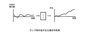
- the differential value of the disturbance is introduced into an evaluation function, and the integrated value is given to the control model after integrating the differential value of the disturbance.
- the present invention having this configuration, even when the disturbance applied to the control model is a ramp, it can be estimated more accurately.
- the control target control method of the present invention is characterized in that the control target is controlled using at least a parameter of the parameter and disturbance estimated by the simultaneous estimation method of the control model parameter and disturbance described above. .
- the present invention since accurate parameters and disturbances are used when controlling the controlled object, it is possible to improve the control performance. That is, in the present invention, the feedback compensation, feedforward compensation, gain table, and the like are optimized based on the control model and disturbance, so that the control performance can be improved.
- MV manipulated variable
- the disturbance and the parameter can be estimated simultaneously and more accurately.
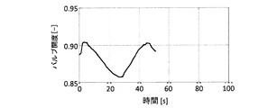
- FIG. 4 is a diagram showing estimated disturbances and simulation results, and is a diagram showing a relationship between a valve opening degree with respect to time (s) during control by a controller B; It is the figure which showed the estimated disturbance and the simulation result, and is the figure which showed the relationship of the hot_water
- FIG. 4 is a diagram showing estimated disturbances and simulation results, and is a diagram showing a relationship between a valve opening degree with respect to time (s) during control by a controller B; It is the figure which showed the estimated disturbance and the simulation result, and is the figure which showed the relationship of the hot_water
- FIG. It is the figure which showed the estimated disturbance and the simulation result, and is the figure which showed the relationship of the hot_water
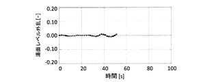
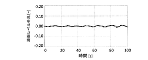
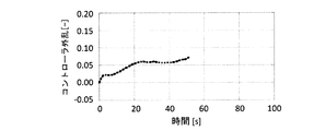
- FIG. It is the figure which showed the estimated disturbance and the simulation result, and is the figure which showed the relationship of the disturbance of the molten metal surface level with respect to time (s) at the time of control by the controller A.
- It is the figure which showed the estimated disturbance and the simulation result and is the figure which showed the relationship of the disturbance of the molten metal surface level with respect to time (s) at the time of control by the controller B.
- FIG. 1 shows a control model when the object is a continuous system.
- control model refers to a representation of a dynamic object that follows the laws of nature so that it can be simulated.
- the control system for the top pressure of the blast furnace 17 is expressed by a state equation (including time integration calculation for obtaining the mass of gas), a flow rate characteristic of a valve, a control switching function, etc.
- the hot water level control system of the continuous casting machine 30 is represented by an integrator, a first-order delay, or the like.
- This control model is expressed by a continuous system shown below or expressed by a discrete system described later.
- the control model may include not only differential equations but also differential algebraic equations.
- the control model may be not only a lumped parameter system but also a distributed parameter system.
- Such a control model can be created using, for example, Simulink (Simulink is a registered trademark of The MathWorks, Inc.), which is public software, The MathWorks, Inc.
- Simulink is a registered trademark of The MathWorks, Inc.
- An example of the continuous control model is shown in equations (1) to (4).
- each variable and each function are as follows.
- t indicates time.
- x (t) is an mx ⁇ 1 vector of a time series function.
- the component indicates a function of all the state quantities in the control model that can be simulated.
- the state quantity is a minimum subset of the system variable group that can represent the state of the entire system at an arbitrary time. For example, in the case of a linear system, it becomes an output signal of the integrator. It is also sometimes called a state variable.
- state quantities In the field of automatic control, these state quantities often represent state quantities to be controlled, but in the present invention, they represent state quantities of all the components of the control model. In other words, in the present invention, in addition to the state quantities to be controlled, the state quantities of the controllers 7 to 9 and 40, and the state quantities of filters and integrators added at the time of optimization are included as necessary.
- x0 is a vector of m x rows and 1 column, and is an initial value of x (t).
- r (t) is a vector of m r rows and 1 column of the time series function.
- known inputs are shown among the inputs applied to the control model.
- Each component is, for example, a target value, a known disturbance, a known value that affects the control model (for example, a steady blast furnace gas flow rate in the top pressure control of the blast furnace 17, that is, a nominal blast furnace gas flow rate, The casting speed of the continuous casting machine 30).
- d (t) is an md ⁇ 1 vector of a time series function.
- Each component is a function of unknown input among the inputs applied to the control model, that is, a variable indicating disturbance.
- p is a vector of m p rows and 1 column, and is a parameter to be adjusted.
- the gain, time constant, dead time, steady value, initial value of state quantity, etc. included in the control model are included as necessary for adjustment.
- these gains can be included.
- p is a time-series value, it can be a parameter that changes with time. Furthermore, it is possible to use a polygonal line gain according to the deviation as a parameter.
- y (t) is the vector of m y rows and one column of the time series function.
- Each component is a function of a variable with which time-series performance data is obtained and matched with data of a time-series simulation result.
- variables for example, in the case of process control, there are an operation amount and a control amount.
- time-series performance data is obtained and there is a variable to be matched with the data of the time-series simulation result, it may be added.
- dd (t) is a vector of m d rows and one column of the time series function. Each component is a function of a variable after an operation such as a filter or integration is performed on the disturbance d (t). For components that do not require an operation such as a filter, interpolation or the like may be performed as necessary, and d (t) may be used as it is as dd (t).
- fc () is a control model for calculating a state quantity in a continuous system. For example, in the case of a linear system, it is composed of three elements, each of which includes a differential equation (including a differential algebraic equation), an output equation, and an expression for operating a filter, an integral, etc. against disturbance. Become.
- cc ineq () is a vector of functions of m ccineq rows and 1 column, and is an inequality constraint expression.
- cc eq () is a vector of functions of m c ceq ⁇ 1 column, and is an equality constraint expression.
- the control model is not particularly limited as long as it is a model that can be simulated with r (t) and d (t) as inputs and y (t) and dd (t) as outputs.
- Fig. 2 shows the control model for discrete systems.
- An example of a discrete control model is shown in equations (5) to (8).
- each variable and each function are as follows.
- the simulation result is stored at the same time interval as the actual data.
- a state quantity is the smallest subset of system variables that can represent the state of the entire system at any given time. For example, in the case of a linear system, the output signal is a delay element z- 1 indicating a delay in the sampling period. In the field of automatic control, these state quantities often represent state quantities to be controlled. In the present embodiment, these state quantities represent state quantities of all the components of the control model. That is, in the present embodiment, in addition to the state quantities to be controlled, the state quantities of the controllers 7 to 9 and 40, and the state quantities of filters and integrators added at the time of optimization are included as necessary. To do.
- x0 is a vector of m x rows and 1 column, and is an initial value of x i .
- Each component has a count i, for example, a target value, a known disturbance, a known value that affects the control model (for example, a steady-state blast furnace gas flow rate in the top pressure control of the blast furnace 17, that is, a nominal value. Blast furnace gas flow rate, casting speed of the continuous casting machine 30) and the like.
- Each component represents an unknown, i.e. disturbance, of the inputs applied to the control model at count i.
- p is a vector of m p rows and 1 column, and is a parameter to be adjusted.
- the gain, time constant, dead time, steady value, initial value of state quantity, etc. included in the control model are included as necessary for adjustment.
- these gains can be included.
- p is a time-series value, it can be a parameter that changes with time. Furthermore, it is possible to use a polygonal line gain according to the deviation as a parameter.
- Each component is a variable that matches the time-series performance data and the data of the time-series simulation result with the count i. For example, in the case of process control, there are an operation amount and a control amount. In addition, if time-series performance data is obtained and there is a variable to be matched with the data of the time-series simulation result, it may be added.
- the corresponding component of dj may be used as the component of dd i .
- fd () is a control model for calculating a state quantity in a discrete system, and corresponds to the above-described continuous system fc ().
- cd ineq () is a vector of functions of m cdineq rows and 1 column, and is an inequality constraint expression.
- cd eq () is a function vector of m cdeq ⁇ 1 column, and is an equality constraint equation.
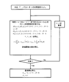
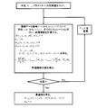
- FIG. 3 is a flowchart of the method for simultaneously estimating the parameters of the control model and the disturbance according to the present invention.
- optimization of parameters and disturbances will be described by taking the case of a discrete control model as an example, but the same process is performed in the case of a continuous control model.
- the conversion from the continuous control model to the discrete control model can be performed using a known method, for example, bilinear conversion or zero-order hold.
- the initial value of the disturbance dj and the initial value of the parameter p are set.
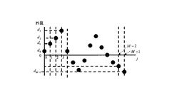
- M functions that are 1 for j and 0 for j are selected as the basis function of the disturbance.
- the orthogonal function such as a discrete Fourier transform and discrete wavelet transform may be selected as the base.
- a linearly independent function may be selected as the basis.
- the simulation can be performed using, for example, Simulink made by The MathWorks, Inc. (Simulink is a registered trademark of The MathWorks, Inc.), which is public software.
- each variable is as follows.
- Each component is a variable of the actual data at the count i when the time-series actual data and the data of the time-series simulation result are matched.
- y i is a variable of simulation result data.
- W y is a matrix of m y rows m y column shows the time series of actual data, the weight of the case to match the time series of the simulation result data.
- a symmetric quasi-positive definite matrix is used.
- W dd is a matrix of m d rows and m d columns, and indicates the weights of variables after operations such as filtering and integration are performed on the disturbance.
- a symmetric quasi-positive definite matrix is used.
- the optimization calculation is performed using a known method, for example, a sequential quadratic programming method.
- Optimization Toolbox is a registered trademark of The MathWorks, Inc.
- Matlab is a registered trademark of The MathWorks, Inc. manufactured by The MathWorks, Inc. It is good to do.
- the evaluation function J does not converge as a result of the optimization calculation, d j and p are changed, and the simulation and the calculation of the evaluation function J are repeated again. If the evaluation function J has converged as a result of the optimization calculation, the obtained d j is set as the optimum value d j opt of the disturbance, p is set as the optimum value p opt of the parameter, and the calculation is terminated.
- a plurality of combinations of the initial value of the disturbance dj and the initial value of the parameter p are set, the flow of FIG. 3 is executed, and the disturbance when the value of the evaluation function is the smallest
- the optimal value d j opt and the optimal parameter value p opt may be adopted.
- FIG. 3 is a flowchart assuming a known sequential quadratic programming method or the like, but other optimization methods such as a known GA (Genetic algorithm) and PSO (Particle Swarm Optimization) may be used. Further, the control system can be designed using the obtained optimum value d j opt of the disturbance and optimum value p opt of the parameter.
- GA Genetic algorithm
- PSO Particle Swarm Optimization
- control parameters of PID control are adjusted by using the results obtained by the method of simultaneous estimation of the parameters of the control model and the disturbance of the present embodiment in the methods of Patent Document 12 and Non-Patent Document 5 described above. Can do. Even in the case of a controller other than the PID control, similarly, the control parameter can be adjusted by using the result obtained by the simultaneous estimation method of the parameter of the control model and the disturbance according to the present embodiment.
- this program is implemented in public software such as Simulink Control Design (Matlab is a registered trademark of The MathWorks, Inc.) such as Matlab (Matlab is a registered trademark of The MathWorks, Inc.) manufactured by The MathWorks, Inc.
- the control parameter can be adjusted by applying the simultaneous estimation method of the parameter of the control model and the disturbance.
- feedforward compensation can be performed using a known method.
- the disturbance input to the controlled object is given to the control model as a time series variable value, and the time series value of the actual data in the controlled object and the simulation obtained by simulating the control model.
- the present invention provides the control model with the disturbance input to the controlled object as a time series variable value, and the simulation result obtained by simulating the time series value of the actual data in the controlled object and the control model This is a method of simultaneously estimating the disturbance and the parameters of the control model so that the evaluation function including the time series value of the data and the time series variable value of the disturbance is maximized or minimized.
- At least one of the controlled variable (PV) and the manipulated variable (MV) is given to the evaluation function as actual data and simulation result data.
- the disturbance after applying the filter that cuts the frequency component is included in the evaluation function.
- parameters having parameters common to all groups of actual data and parameters having values linked to each group of actual data are introduced into the evaluation function as time series variable values linked to each group of the actual data.
- unknown initial values are employed as the above parameters.
- unknown steady values are employed as the above parameters.
- the control target can be controlled by using at least the parameter and the parameter estimated by the simultaneous estimation method of the parameter and the disturbance of the control model according to the present invention.
- a method for controlling a controlled object using the simultaneous estimation method for parameters and disturbances of the control model of the present embodiment will be described with three specific examples.
- the first example is a method for determining the feedforward compensation amount by simultaneously estimating the disturbance and the parameter for the operation method of the bypass valves 6a and 6b in the top pressure power generation facility 1 of the blast furnace 17 which is one of steel processes. explain.
- the furnace top pressure power generation facility 1 of the blast furnace 17 collects gas (blast furnace gas) discharged at the furnace top of the blast furnace 17 and generates power using the collected blast furnace gas.
- a blast furnace gas flow path 4 for collecting gas is provided.
- the blast furnace gas flow path 4 is connected to a dust collection facility for removing dust contained in the blast furnace gas.
- This dust collection equipment is a dust catcher (not shown) or a ring slit washer (RSW), and dust and the like can be removed by passing blast furnace gas through these.
- the ring slit washer (RSW) is configured by connecting a plurality (for example, three) of ring slit elements 2 (RSE) in parallel.
- the blast furnace gas flow path 4 on the downstream side of the RSE 2 is provided with a mist separator (not shown) and is branched into at least two flow paths.
- the first flow path is a main flow path that passes through the power generation unit 3 (TRT) that generates power with blast furnace gas, and the second flow path is between the gas inlet side and the gas outlet side of the TRT 3.
- TRT power generation unit 3
- It is a bypass channel that is connected separately from the main channel.
- the bypass channel 5 is provided with two bypass valves 6a and 6b in parallel.
- a silencer 18 for silencing the blast furnace gas is provided on the downstream side of the bypass flow path where the bypass valves 6a and 6b are installed.
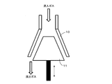
- the RSE 2 includes a conical tube 10 through which a blast furnace gas flows, and a movable cone-shaped (conical) movable portion 11 inserted into the conical tube 10.
- the movable part 11 is controlled by the furnace top pressure controller 7 shown in FIG. Specifically, the furnace top pressure controller 7 obtains the operation amount of the movable part 11 based on the actual value of the furnace top pressure and the target value of the furnace top pressure, and moves the movable part 11 based on the operation amount. Let That is, the furnace top pressure controller 7 operates the interval between the conical tube 10 and the movable part 11 and adjusts the flow rate of the blast furnace gas to pass so that the furnace top pressure becomes a target value.
- the flow rate and pressure of the blast furnace gas are adjusted by changing the gap between the two by the valve mechanism 16a configured by the movable portion 11 and the conical tube 10 (case).
- the inflowing gas contains fine water droplets, and when passing through the gap, the flow velocity increases, so that fine dust and water droplets can adhere and be removed.
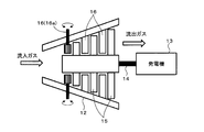
- the TRT 3 power generation unit
- the TRT 3 includes a moving blade 15 provided on a shaft 14 (rotor) of a turbine directly connected to the generator 13, and a stationary blade 16 fixed to the casing 12 side. Yes.
- a part of the stationary blade 16 is configured by a blade valve 16a (valve mechanism) whose angle can be changed, and the blade angle (valve angle) is changed by the TRT pre-pressure controller 8 shown in FIG. It can be done.
- the TRT pre-pressure controller 8 obtains the operation amount of the blade valve 16a and the like based on the actual value of the pre-pressure and the target value of the pre-pressure, and changes the angle of the blade valve 16a based on the operation amount.
- the gas flow rate passing through the TRT 3 is adjusted so that the pre-pressure becomes the target value.
- the blast furnace gas which is an inflow gas
- the moving blade 15 rotates the shaft 14 of the turbine.
- the turbine shaft 14 is connected to a generator 13 and generates power.
- the foremost stationary blade 16 is a blade valve 16a whose angle can be changed, and the flow rate and pressure of the blast furnace gas can be adjusted.
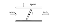
- the bypass valves 6 a and 6 b are valves called butterfly valves, and the degree of opening of the bypass valve (valve is changed by rotating the circular disk around the axis to change the angle. Can be changed.
- the bypass valve pre-pressure controller 9 shown in FIG.
- the flow rate of gas passing through the bypass channel 5 is adjusted, that is, the pre-pressure is controlled to the target value.
- the first bypass valve 6a has a valve opening controlled by feedforward compensation (FF compensation), and the second bypass valve 6b has a combination of feedforward compensation (FF compensation) and feedback compensation (FB compensation).
- the valve opening is controlled.
- 5 shows an example in which two bypass valves 6a and 6b are installed in the bypass channel 5, but the present invention is not limited to this example, and one bypass valve is provided in the bypass channel, or Three or more may be installed. Further, the bypass valves 6a and 6b may be valves other than the butterfly valve. Further, when there is no furnace top pressure control system such as RSE2, the TRT 3 and the bypass valves 6a and 6b control the furnace top pressure.
- the blast furnace gas discharged from the furnace top of the blast furnace 17 normally flows through the TRT 3 and is then recovered to the blast furnace gas holder.
- the turbine is rotated by blast furnace gas to generate power.
- the bypass valves 6a and 6b are controlled by normal FF compensation and FB compensation.
- the CV values of the bypass valves 6a and 6b are set so that the flow rate by the feedforward compensation of the bypass valves 6a and 6b becomes equal to the flow rate of the blast furnace gas flowing in the power generation unit 3 obtained by calculation. And calculating the feedforward compensation amount of the opening degree of the bypass valves 6a and 6b, and applying the calculated feedforward compensation amount to the bypass valves 6a and 6b, so that the blast furnace gas at the time of emergency stop can be used as the bypass valves 6a and 6b. Trying to escape to the side.
- the parameters in the control model and the disturbances input to the control target (bypass valves 6a and 6b) represented by the control model are estimated at the same time.
- To obtain an accurate feedforward compensation amount the processing at the time of emergency stop will be described in detail when the flow rate flowing through the bypass valves 6a and 6b is 0 (zero) before the TRT emergency stop.
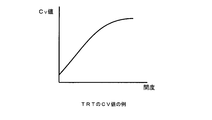
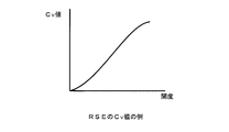
- the CV value will be described. 9-11, respectively, show examples of TRT3, the bypass valve 6a, 6b, C V values or C V value corresponding value of RSE2.
- the opening is an angle of the blade valve 16a, an angle of the butterfly valve, and a gap (displacement amount) in the valve mechanism 16a (the movable portion 11 and the conical tube 10) in the RSE2.
- the opening degree may be expressed as a percentage by normalizing the angles and displacements of TRT3, bypass valves 6a, 6b, and RSE2.
- the characteristics of the CV values of the bypass valves 6a and 6b are the same.
- the characteristics of the CV values of the bypass valves 6a and 6b may be different.
- the CV value is calculated according to the P.A. of the publicly known literature “Revised 2nd edition, practical handbook of industrial process control valves, Yamatake Corporation, control valve handbook compilation committee, Nihon Kogyo Shuppan, 2012”. As described in 52, this is a value called a capacity coefficient, and is a numerical value expressed by [USgal / min], which is a volume flow rate through which water having a specific gravity of 1 passes as a valve differential pressure of 1 [psi].
- the CV value in the present invention is at least the opening degree of the valve mechanism (blade valve 16a, bypass valves 6a, 6b, RSE2, etc.), the inlet pressure, and the fluid flowing through the valve mechanism 16a. Any value may be used as long as it indicates the relationship with the flow rate, and the flow rate can be obtained from the opening, or the opening can be obtained from the flow.
- the CV value in the present invention includes a value corresponding to the CV value.
- the pressure on the outlet side of the valve mechanism 16a, the temperature of the fluid, and the like may or may not be used in an expression indicating the relationship with the flow rate of the fluid flowing through the valve mechanism 16a. In the following description, it is not necessary to input an unused value. Further, the pressure on the inlet side or the pressure on the outlet side of the valve mechanism 16a includes the pressure when the pipes and the silencer 18 constituting the flow path are included.
- the bypass valve 6b is compensated for feedback so that the previous pressure target value and the previous pressure actual value coincide with each other, and until the gas having the same flow rate as the gas flowing in the TRT 3 flows to the bypass valves 6a and 6b. 6b will be opened.
- the flow rate of the bypass valve 6 is smaller than the flow rate flowing to the original TRT 3 until the opening degree of the bypass valve 6 reaches a steady value. For this reason, as shown in FIG. 12, the mass of the blast furnace gas between RSE2 and a bypass valve will increase, and the pressure of this part, ie, a pre-pressure, will increase temporarily. Furthermore, when the pre-pressure (in other words, the back pressure of RSE2) increases, the flow rate flowing through RSE2 temporarily decreases, the mass of the blast furnace gas between blast furnace 17 and RSE2 increases, and the top pressure also increases. Will increase.
- FIG. 13 shows a block diagram of control of the bypass valves 6a and 6b of the present invention.
- the feedforward compensation amount to the bypass valves 6a and 6b is quantitatively determined using the CV value of the TRT3 and the CV values of the bypass valves 6a and 6b.
- the feedforward compensation amount is applied only to one bypass valve, but in the present invention, the feedforward compensation amount is applied to a plurality of bypass valves 6a and 6b.
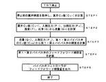
- FIG. 14 is a flowchart for obtaining the feedforward compensation amount.
- the bypass valves 6a and 6b are closed, and the entire amount of blast furnace gas flows to the TRT3 side.
- the opening degree of the blade valve 16a (referred to as the blade valve opening degree) is acquired, and the CV value (referred to as the blade valve CV value) of the blade valve 16a is calculated according to FIG. This is STEP1 in FIG.
- Each parameter P 1 , P 2 , T, G, a T is an actual value obtained from a sensor or the like, a value obtained from a simulation, a value provided by the manufacturer of the bypass valves 6a and 6b itself, or the like. This is a value obtained by unit conversion in accordance with non-dimensionalization. Then, after calculating Tsubasaben C V values the flow rate of (C VT) and blast furnace gas (Q T), calculates the opening degree of the bypass valve 6a, 6b. This is STEP 3 in FIG.
- the opening degree of one bypass valve (second bypass valve 6b) is provisionally determined and the opening degree of the other bypass valve (first bypass valve 6a) is obtained.
- first bypass valve 6a the opening degree of the second bypass valve 6b is 42%.
- the characteristics of the first bypass valve 6a and the characteristics of the second bypass valve 6b are the same and have the characteristics shown in FIG.
- CV value (C VB ) of bypass valves 6a and 6b, flow rate of bypass valves 6a and 6b (Q B [ ⁇ ]), inlet side pressure (pre-pressure) of bypass valves 6a and 6b (P 1 [ ⁇ ]), Equation (11) is established for the temperature (T [° C.]) of the blast furnace gas flowing through the bypass valves 6a and 6b.
- Each parameter P 1 , T, G, a B is an actual value obtained from a sensor or the like, a value obtained from a simulation, a value provided by the manufacturer of the bypass valves 6a and 6b itself, or dimensionless. It is a value that is unit-converted according to conversion. Because the degree of opening of the second bypass valve 6b is 42%, it is possible to obtain a C VB2 from relationship opening and CV value (C VB), a C V value of the second bypass valve 6b shown in FIG. 10 . Then, CVB2 obtained in FIG. 10 and T, P 1 , G, a B can be substituted into Expression (11) to obtain Q B2 that is the flow rate of the second bypass valve 6b.
- the characteristics of the first bypass valve 6a are the same as those of the second bypass valve 6b.
- the first bypass valve 6a can be used for the first bypass valve 6a.
- C VB1 that is the C V value to be obtained can be obtained.
- the opening degree of the first bypass valve 6a can be obtained using CVB1 obtained by the equation (11) and FIG.
- each flow rate is a non-dimensional flow rate [Nm 3 / h] in a standard state or a non-dimensional mass flow rate [kg / s].
- the feedforward compensation amount of the bypass valves 6a and 6b is calculated. This is STEP4 in FIG.
- “feed forward compensation amount calculated opening”.
- the bypass valve pre-pressure controller 9 When the setting of the feedforward compensation amount is completed, the bypass valve pre-pressure controller 9 outputs the feedforward compensation amount. This is STEP5 in FIG.
- the power generation unit 3 includes the valve mechanism 16a (wing portion) that can adjust the flow rate (Q T ) of the blast furnace gas flowing in the power generation unit 3.
- the flow rate of the blast furnace gas before emergency stop of the power generation unit 3 is calculated based on the opening degree of the valve mechanism 16a and the CV value.
- FIG. 15 shows the result when the present invention is implemented, which is an ideal control situation.
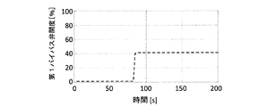
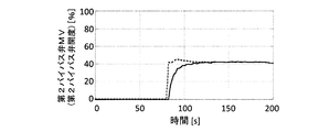
- the feedforward compensation amount of the second bypass valve 6b (the lowest stage in FIG. 15) and the feedforward compensation amount of the first bypass valve 6a (second from the bottom in FIG. 15) are optimized.
- the entire amount of blast furnace gas that has flowed to the TRT 3 side will immediately flow to the bypass flow path by feedforward compensation.
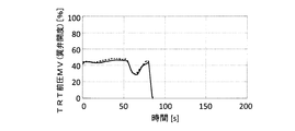
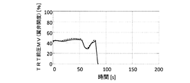
- variation of a pre-pressure (2nd from the top in FIG. 15) is suppressed, and also the fluctuation
- the accuracy of the CV value of the power generation unit 3 and the CV values of the bypass valves 6a and 6b affects the accuracy of the feedforward compensation amount.
- the CV value of the power generation unit 3 is influenced by the pipes 4 and 5, the influence of the upstream / downstream equipment (such as the silencer 18), and the influence of the temporal change of the furnace top pressure power generation equipment 1 (gas component, piping) Change). Therefore, C V value of the power generation unit 3 to be used when calculating the feedforward compensation amount, and the bypass valve 6a, for C V value 6b, nominal values (manufacturer provides the values, when installing equipment Calculated etc. ) Need to be corrected.
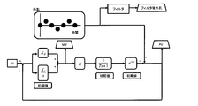
- FIG. 16 shows a control model of the furnace top pressure and the pre-pressure.
- the furnace top pressure and pre-pressure control models correspond to equations (1) and (2) that are continuous control models, but in reality, Simulink made by The MathWorks, Inc., which is public software. (When Simulink is a registered trademark of The MathWorks, Inc.), it is discretized and corresponds to Equations (5) and (6).
- the equation of state between the blast furnace and the RSW is as follows.
- the mass of the blast furnace gas is obtained by time integration of “blast furnace gas flow rate at the top of the furnace ⁇ blast furnace gas flow rate at the RSE”.
- the equation of state between the RSW and the inlet is as follows.
- the mass of the blast furnace gas is obtained by time integration of “blast furnace gas flow rate at RSE ⁇ blast furnace gas flow rate at TRT ⁇ blast furnace gas flow rate at the first bypass valve ⁇ blast furnace gas flow rate at the second bypass valve”.
- the output from the furnace top pressure controller 7 corresponds to the opening of the furnace top pressure MV or RSE2.
- the output from the TRT pre-pressure controller 8 corresponds to the TRT pre-pressure MV or the blade valve opening.
- the output from the bypass valve pre-pressure controller 9 corresponds to the bypass valve pre-pressure MV or the bypass valve opening.
- the furnace top pressure SV is a furnace top pressure target value
- the pre-pressure SV is a pre-pressure target value.
- the nominal CV value shown in FIG. 11 is used as the RSE nominal flow rate characteristic.
- the CV value on the vertical axis in FIG. 11 indicates the flow rate [1 / s] itself.
- the flow rate is the flow rate in the standard state or the mass flow rate, but the mass is made dimensionless as described above. If the furnace top pressure MV is input, the flow rate of RSE2 is output.
- the nominal CV value shown in FIG. 9 is used as the TRT nominal flow rate characteristic. Enter the TRT before pressure MV, it obtains a C V value, since the C V value and the formula (10), the flow rate of TRT3 is output.
- the nominal CV value shown in FIG. 10 is used as the second bypass valve flow rate characteristic. The bypass valve pre-pressure MV is input, the CV value is obtained, and the flow rate of the second bypass valve 6b is output from the CV value and Expression (11).
- the nominal CV value shown in FIG. 10 is used as the first bypass valve flow rate characteristic.
- the FF compensation amount is input, the CV value is obtained, and the flow rate of the first bypass valve 6a is output from the CV value and Expression (11).
- the nominal flow rate is a known nominal blast furnace gas flow rate. This nominal flow rate is a constant value of the blast furnace gas flow rate and is a constant value. A disturbance is applied to the steady value when the raw material is charged.
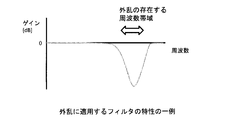
- the filter of this specific example employs a filter having a large gain in the low frequency region and a small gain in the high frequency region as shown in FIG.
- This filter is designed to reduce the gain in a high frequency region where disturbance exists.
- a first-order lag filter with a time constant of 100 [s] is used.
- the corner frequency is 1.59 ⁇ 10 ⁇ 3 [Hz] (period 628 [s]).
- the filter by applying the filter to the disturbance to be estimated, the high-frequency disturbance is reduced in the signal after the filter is applied, and the reduced high-frequency disturbance is not evaluated by an evaluation function described later. That is, by using the above-described filter, the value of the high-frequency disturbance before applying the filter can be increased and can be estimated at the time of optimization.
- the low-frequency disturbance signal is not attenuated, and therefore is evaluated by an evaluation function described later.
- the value of the low-frequency disturbance before the filter application becomes a small value by optimization.
- disturbances in the high frequency region are estimated as large values as disturbances.
- K CR, K CB2, K R, K T, K B is to be estimated, which is a parameter of the control model.
- K CR and K CB2 assume a case where the PID controllers 7 and 9 have an unknown gain.
- K R , K T , and K B are assumed to require correction coefficients for the characteristics of RSE2, TRT3, and bypass valves 6a and 6b.
- the blast furnace gas flow rate disturbance is a disturbance mainly showing a fluctuation that the flow rate of the blast furnace gas decreases when iron ore or coke is charged (charged) into the blast furnace 17.
- the blast furnace gas flow rate disturbance includes a change in the blast furnace gas flow rate due to a turbulence of the gas flow in the blast furnace 17 or the like.
- the value of the blast furnace gas flow rate disturbance with a count corresponding to the value at each time in the time series is a variable.
- the subscript “actual result” means an already obtained actual value
- “simulation” means a simulation value.
- the first term to the fifth term of the equation (18) are terms for making the simulation value coincide with the actual value for y i , specifically, the control amount (PV) and the operation amount (MV). This is a term for matching results and simulations.
- the sixth term of Equation (18) is a term for bringing the disturbance after applying the filter close to 0 (zero).
- Constraint conditions are as follows and correspond to equation (7).
- furnace top pressure control in this specific example is a form that embodies the general form. Next, the furnace top pressure control in this example will be specifically described.
- x0 (initial value) is not a variable but a fixed value.
- the initial value of the mass of the blast furnace gas between the top of the furnace and the RSW, and the initial value of the mass of the blast furnace gas between the RSW, the TRT 3 and the bypass valves 6a and 6b are the pressure, volume, Since the temperature is known, the calculated value is obtained from the equation of state.
- r i The components of r i (known input) are nominal blast furnace gas flow rate, furnace top pressure target value (SV), pre-pressure target value (SV), blast furnace gas temperature at the location where the temperature is used, TRT3 / bypass valve 6a. , 6b back pressure, and FF compensation amount (in the conventional control).
- m r 6.
- d j (unknown input) is the disturbance to be estimated and is the blast furnace gas flow disturbance applied to the nominal blast furnace gas flow.
- m d 1.
- M 41.
- the components of y i are the furnace top pressure control amount (PV), the pre-pressure control amount (PV), the furnace top pressure manipulated variable (MV), and the TRT pre-pressure manipulated variable (MV). ), The operation amount (MV) of the bypass valve pre-pressure.
- m y 5.
- dd i value after performing an operation such as filter or integration on the disturbance
- m d 1. fd () is a control model for calculating a state quantity in a discrete system, and is a model obtained by discretizing the model shown in FIG.
- Simulink Simulink is a registered trademark of The MathWorks, Inc.
- the MathWorks, Inc. which is public software, is used for discretization and calculation.
- weights of the evaluation function are as shown in the following equations (20) and (21), respectively.
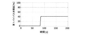
- the actual value is used for the feedforward amount of the first bypass valve 6a.
- the blade valve opening is set to 0 (zero) which is the same value as the actual result after the trip.
- the shut-off valve in front of TRT3 is closed so that the flow rate flowing through TRT3 becomes zero, so the flow rate flowing through TRT3 is set to zero.
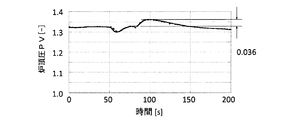
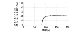
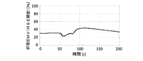
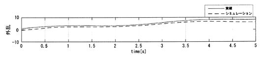
- the blast furnace gas flow rate disturbance at this time is estimated as shown in the graph (thick broken line) shown in FIG. 18F. It can be seen that the steady-state deviation of the disturbance is almost 0 (zero), and the disturbance in the high frequency region having a period of about 20 seconds is estimated. 18A to 18E and FIG. 18G show other performance data (solid line) and simulation result data (broken line). As described above, the accurate feedforward compensation amount can be obtained by correcting the CV value based on the equation (22).
- FIG. 19 shows data of a simulation result when accurate feedforward compensation is applied.
- the already estimated disturbance is used for the simulation.
- the parameters already estimated are used.
- 19A to 19E and FIG. 19G show other result data (solid line) and simulation result data (broken line).
- the target furnace top pressure is 1.325 [ ⁇ ]
- the fluctuation of the furnace top pressure is It can be seen that 0.036 in FIG. 18A is reduced to 0.011 in FIG. 19A.
- the PID controllers 7 to 9 can be used for gain adjustment of the PID controllers 7 to 9 by using the above-described simultaneous estimation method.
- a gain that does not saturate can be selected for the magnitude and speed of the manipulated variable (MV) affected by the disturbance.
- the estimated disturbance can be used for equipment diagnosis and the like.
- controller design such as H ⁇ control and observer.
- FIG. 20 shows a result of an example in which the second bypass valve 6b is gradually closed while the first bypass valve 6a is closed.
- the estimated disturbance is shown in the graph of FIG. 20F (thick broken line). It can be seen that the steady-state deviation of the disturbance is almost 0 (zero), and a high-frequency disturbance having a period of about 40 seconds is estimated.
- 20A to 20E and FIG. 20G show other actual values (solid lines) and simulation results (broken lines).
- K CB2 may be set as follows using cd eq () (equal constraint equation).
- parameters and disturbances can be appropriately estimated by changing the simulation conditions and changing the parameters to be estimated in accordance with the operation conditions.
- the disturbance and parameters are estimated simultaneously to identify the cause of the control deviation. Further, a method for adjusting the control system will be described.
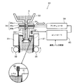
- a molten steel hole 34 through which the molten steel X in the tundish 33 is discharged to the mold 31 is formed at the bottom of the tundish 33.
- An immersion nozzle 35 is provided so as to communicate with the molten steel hole 34, and the tip of the immersion nozzle 35 is inserted into the mold 31.
- a slide valve 36 for adjusting the flow rate of the molten steel X flowing down in the immersion nozzle 35 is provided at the bottom of the tundish 33 and at the root of the immersion nozzle 35 so as to be adjacent to the molten steel hole 34.
- the slide valve 36 has a fixed plate-like upper plate 36a and lower plate 36b made of a fixed refractory, and a moving plate-like intermediate plate 36c made of a fixed refractory.
- the lower surface of the upper plate 36a and the upper surface of the intermediate plate 36c are in surface contact, and the upper surface of the intermediate plate 36c slides in the horizontal direction on the lower surface of the upper plate 36a.
- the relationship between the lower plate 36b and the intermediate plate 36c is the same as the relationship between the upper plate 36a and the intermediate plate 36c, except that the vertical positional relationship is different.
- the upper plate 36a, the lower plate 36b, and the intermediate plate 36c are provided with flow-down holes 37 (valves) through which the molten steel X that passes through in the vertical direction and is discharged from the tundish 33 is passed.
- the intermediate plate 36c is connected to an electrohydraulic cylinder 39 (actuator) whose rod extends and contracts in the horizontal direction.
- the intermediate plate 36c By extending and contracting the rod of the electrohydraulic cylinder 39, the intermediate plate 36c includes an upper plate 36a and a lower plate 36b.
- the cross-sectional area of the flow-down hole 37 (valve cross-sectional area) changes, and the flow rate of the molten steel X flowing down is variable.
- a hot water level meter 38 for measuring the hot water level in the mold 31 is provided above the mold 31.
- the molten metal level refers to the height of the molten steel surface (molten metal surface) in the mold 31.
- the continuous casting machine 30 includes a control unit 40 (controller) that applies the calculated amount to the slide valve 36.
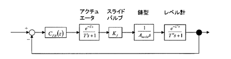
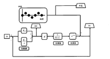
- FIG. 22 is a block diagram of a hot water surface level control system (also simply referred to as a level control system) in the mold 31 performed by the control unit 40.
- C FB (z) is a feedback controller and is a function of the delay element z ⁇ 1.
- the actuator 39 and the molten metal level meter 38 are each represented by “first order delay + dead time”, and are discretized during simulation.
- Simulink (Simulink is a registered trademark of The MathWorks, Inc.) made by The MathWorks, Inc., which is public software, can be used for the simulation.
- Slide valve 36 is represented by the gain of the flow rate coefficient K f.
- the mold 31 is represented by an integrator whose gain is a reciprocal of the mold cross-sectional area A mold .
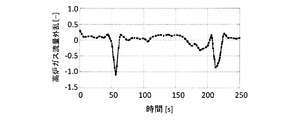
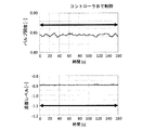
- FIG. 23 shows an example of an abnormal state in which the hot water surface level is hunting with a steady deviation.
- the slide valve opening graph shows the actual value.
- the solid line indicates the actual value (PV of the molten metal surface level control), and the alternate long and short dash line indicates the target value (SV of the molten metal surface level control).
- the controller A controls from time 0 to about 50 seconds.
- the controller B controls between about 50 to 160 seconds.
- hunting with a period of about 40 seconds occurs.
- the hot water surface level target value is -1.02 [-] (dashed line) ([-] indicates a non-dimensional value).
- the actual surface level value oscillates around about ⁇ 0.95 [ ⁇ ], and an offset occurs in the level deviation.
- Possible causes of hunting and steady deviation include disturbance (for example, disturbance due to bulging, etc.), control hunting (for example, control gain is too high, time constant is too long, dead time is too long, control gain is unknown Are present in the loop), hardware abnormal operation (unexpected operation), and the like. However, since both the disturbance and the control system parameters are unknown, it is difficult to identify the cause of the abnormality.
- disturbance for example, disturbance due to bulging, etc.
- control hunting for example, control gain is too high, time constant is too long, dead time is too long, control gain is unknown Are present in the loop
- hardware abnormal operation unexpected operation
- the cause of this level control abnormality is determined by estimating the parameters of the control model and the disturbance applied to the control model.
- the main component of the disturbance at the molten metal surface level is a disturbance (bulging disturbance) caused by the solidified shell called bulging bulging or denting between the rolls 32 below the mold 31 to change the height of the molten metal surface of the mold 31.
- the frequency of this disturbance is casting speed / roll 32 spacing.
- the filter c in FIG. 24 is a filter applied to the differential value of the disturbance applied to the controller 40 (the differential value of the controller disturbance) as shown in FIG.
- the shape of the filter is the same as in FIG.
- the estimation is based on the assumption that the differential value of the disturbance includes a component having a period of around 13.5 seconds. As will be described later, as a result, it was estimated that there was no controller disturbance of this period. That is, it was confirmed that the disturbance in the vicinity of the period of 13.5 seconds is a molten metal level disturbance. As shown in FIG. 27, the disturbance applied to the controller 40 is integrated, and a ramp-shaped disturbance can be expressed.
- the case where the control is performed by the controller A (40) and the case where the control is performed by the controller B (40) are extracted as different data. That is, there are a plurality of groups of time-series values of performance data. In this example, there will be two groups. Controllers A and B (40) are expressed by the following equations.
- z ⁇ 1 means a delay element of the sampling period as described above.
- Z-nod means a delay element of time corresponding to the nod sampling period.
- each coefficient is known and has the following value.
- u 1init_k , u 2init_k , u are respectively set to z ⁇ 1 , z ⁇ 2 , z ⁇ 3 , and z ⁇ 4 of the numerator of Expression (25) as initial values of the respective delay elements of the denominator.
- the flow coefficient / mold cross-sectional area which is the gain to be controlled, was determined as follows.
- the next primary delay means a primary delay component to be controlled, and is expressed by a primary delay “1 / (T lag ⁇ s + 1)”.
- the time constant T lag is a parameter and includes one state quantity.
- the time constant of the actuator 39 is ignored because it is small, and it is assumed that there is a first-order lag between the hot water surface level true value and the hot water surface level observation value.
- This first order delay includes the characteristics of the sensor and the characteristics of the filter added to the sensor. In the simulation, it is discretized and solved as appropriate.
- the gain k plant indicates an unknown gain of the control target, and in this specific example, represents the unknown gain of the entire control target including the fluctuation amount of the flow coefficient Kf and the fluctuation amount due to other dynamic characteristics. k plant is 1 if it matches the control model.
- the operation amount (MV) obtained from the equation (25) is the operation amount for the deviation system, and 0 (zero) is used as a reference. Therefore, a value obtained by adding a steady value in the initial state is a slide valve obtained by simulation. Opening degree.
- the “water surface level target value”, “water surface level”, and “valve opening” shown in FIG. 24 and the like are the “water surface level SV” and “water surface level” of the level control system, respectively.
- k con , T lag , T delay , and k plant are common parameters, and the rest are individual parameters.
- the common parameter is a parameter used as a common value in the model when a plurality of performance data is used.
- it is a parameter having a value common to all groups of performance data.
- An individual parameter is a parameter used as an individual value in a model when using a plurality of performance data. That is, it is a parameter having a value that is linked to each group of performance data.
- the unknown initial value means an unknown value to be given at the initial stage of the simulation.
- the unknown steady value is an unknown value among the steady values to be given when a deviation system is configured as a control system and simulation is performed.
- the value at the count corresponding to the value of each time in the time series is used as a variable.
- the second disturbance is a disturbance that is applied until the control computer outputs the manipulated variable (MV) and then the slide valve opening actually changes.
- the second disturbance is estimated to be a ramp-shaped disturbance because the molten metal surface level has a steady deviation.
- the second disturbance was later confirmed by an investigation as a result of a signal being lost in the operation signal transmission path.
- the differential value of the disturbance is a value at a count corresponding to the value at each time in the time series as a variable.
- two result data are used, that is, the result data when controlled by the controller A (40) and the result data when controlled by the controller B (40).
- the disturbance is separate for each performance data and uses a separate disturbance.
- the individual disturbance is a disturbance that is used as an individual time-series value for each result data when a simulation is performed using a plurality of result data. That is, it is a time series variable value that is linked to each group of performance data.
- the evaluation function of this specific example was determined as follows. In other words, parameters common to models corresponding to two performance data are assumed to be common variables, and different parameters are estimated as different variables. Since disturbances are different, they are estimated separately. Then, the following expression (28) was used as an evaluation function for parameters in the control model.
- the 1st term and the 2nd term are terms for making the hot water level and the valve opening coincide with each other in the actual results and the simulation.
- the sampling period of the result data and the simulation result data is 1 second.
- Constraint conditions of the control model are as follows.
- the hot water level control in this specific example is a specific form of the general form that is expanded when the number of data is one and the number of data is plural.
- x ki state quantity
- x ki state quantity
- Delay element depending on discretization method
- delay element of dead time element number depends on sampling time of discretization
- controller disturbance The number of state quantities depends on the simulation method.
- x0 k (initial value) is an initial value of eight delay elements (numerator 4 + denominator 4) of the controller 40, an initial value of a delay element corresponding to the integrator of the template 31, and a delay element corresponding to an integrator of the first-order delay Is the initial value of the delay element of the dead time element. Note that the initial value of the delay element corresponding to the integrator applied to the differential value of the controller disturbance is zero.
- r ki (known input) is a surface level SV (level target value) corresponding to each k.
- the reason why the time interval of the disturbance variable is longer than 1 second of the sampling period of the actual data and the simulation result data is to allow the disturbance variable to be reduced. For example, when the temporal change of the disturbance is expected to be smooth, the time interval of the disturbance variable can be increased, and the amount of calculation for optimization can be reduced.
- dd ki is a value after a filter or integration operation is performed on the disturbance, a value after applying a low-pass filter to the differential value of the controller disturbance (filtered controller disturbance differential value), and a band stop on the level disturbance It is a value after applying the filter (post-filter level disturbance).
- fd () is a control model for calculating a state quantity in a discrete system, and is a control model obtained by discretization from the model shown in FIG.
- Simulink Simulink is a registered trademark of The MathWorks, Inc.
- the MathWorks, Inc. which is public software
- the discrete equations in this specific example are described on the assumption that they are solved with a fixed sampling period. However, the sampling period may be variable as possible with the above software.
- the integrator in the control model is discretized and calculated in the software.
- the parameter evaluation function in the control model is the following expression (30) obtained by expanding expression (9) corresponding to a plurality of actual data.
- each variable is as follows.
- N is the number of performance data.
- Each component is actual data when the time-series actual data and the simulation result data at the count i are matched.
- W yk is a matrix of m yk rows and m yk columns. Shows the weight of simulation result data.
- W ddk is a matrix of m dk rows and m dk columns. Indicates the weight of the value after operations such as filtering and integration are performed on the disturbance.
- a symmetric quasi-positive definite matrix is assumed. Specific numerical values are as follows.
- the disturbance corresponding to the two performance data at this time is estimated as shown in the graphs (thick broken lines) in FIGS. 29E to 29H.
- the controller disturbance shown to FIG. 29G and FIG. 29H the value after integrating is displayed.
- the estimated level disturbance is small, it is estimated that small bulging occurs in the continuous casting machine 30.
- the bulging disturbance is estimated to have a period of about 13.5 seconds.
- the steady-state deviation of the hot water level disturbance is estimated to be almost 0 (zero). Further, it is estimated that a ramp-like disturbance is applied as the controller disturbance.
- a lamp-like disturbance and a small disturbance having a superimposed period of about 40 seconds are applied as the controller disturbance.
- These disturbances in the frequency band are outside the frequency band where the disturbance differential value is expected to exist, and the disturbance differential value is estimated as a small value.
- the disturbance in the vicinity of the period of about 13.5 seconds expected to exist is not estimated, and the disturbance in the vicinity of the period of 13.5 seconds is assumed to be a level disturbance rather than a controller disturbance.
- the third example is an example in which the evaluation function does not include the time series variable value of the disturbance.
- 1 in the third example is a control object configured by a gain K, a first-order delay of a time constant T, and a dead time L as shown in FIG.
- PI control is used as a controller, a proportional gain K P, the integral gain and K I.
- Laginit_ the initial value of primary delay tv
- delayinit_ the initial value of the dead time tv
- the initial value of the integral element of the controller to Iinit_ tv.
- continuous elements are discretized during simulation. Also, let the disturbance be d (t).
- ⁇ ⁇ Determine the parameters of the control model and the true value of the disturbance as shown in the following equation (36). Note that _tv is a subscript indicating a true value.
- 32A to 32D show the true value parameters and actual data in the case of true value disturbances.
- the true value or the simulation result using the true value is used as the result data.
- the parameters of the control model and the disturbance are back-calculated from the result data.
- the disturbance of the performance data includes a ramp-like disturbance and an offset.
- the subscript “actual result” means an already obtained actual value
- “simulation” means a simulation value
- the first term and the second term of the equation (37) are terms for making the simulation value coincide with the actual value for y i , specifically, the control amount (PV) and the operation amount (MV). ) Is a term for matching the actual results with the simulation.
- x0 (initial value) is the initial value of the state quantity when the integrator of the time constant and the integrator of the PID controller are discretized, and the initial value of the state quantity when the dead time is discretized.
- the component of r i (known input) is a target value (SV).
- m r 1.
- d j (unknown input) is a disturbance to be estimated.
- m d 1.
- M 26.
- y i (variables to be matched)
- y i (variables to be matched)
- m y 2.
- fd () is a control model for calculating a state quantity in a discrete system, and is a model obtained by discretizing the model shown in FIG.
- discretization and calculation are performed using Simulink (Simulink is a registered trademark of The MathWorks, Inc.) made by The MathWorks, Inc., which is public software.
- weights of the evaluation function are as shown in the following formulas (39) and (40), respectively.
- optimization is performed based on the flowchart shown in FIG. It should be noted that the initial value of optimization is given within a range satisfying the constraint condition, and the case where optimization is performed a plurality of times and the value of the minimum evaluation function is 0.00 is adopted. In addition, the initial value at this time is as the following formula (41).
- 33A to 33D show simulation results after optimization.
- SV is giving the same SV as a result at the time of simulation.
- FIGS. 33A to 33D as can be seen from the evaluation function value being 0.00, for PV and MV, the actual results and the time series values of the simulation match.
- the parameter of the obtained control model is as the following formula (42).
- the estimated disturbance coincides with the actual disturbance.
- the evaluation function further includes a time series variable value of disturbance in the first example of the third example, that is, the third example 2
- the reason for studying is that, as in the case of the second example, accurate parameters and disturbances cannot be estimated unless the time series variable values of disturbances are evaluated.
- Equation (43) is a term for bringing the disturbance closer to 0 (zero). Further, the constraint conditions are the same as those in the equation (38).
- this example is a form that embodies the general form. Only the difference from 1 in the above-described third example will be described below.
- dd i has the same value as the disturbance d j at the same time. In order to obtain dd i from dj , interpolation or the like may be performed.
- Equation (39) The weight of the evaluation function is as shown in Equation (39) and Equation (44) below, respectively.
- optimization is performed based on the flowchart of FIG. It should be noted that the initial value of optimization is given within a range that satisfies the constraint conditions, and the case where optimization is performed a plurality of times and the value of the minimum evaluation function is 1.19 ⁇ 10 4 is employed. In addition, the initial value at this time is as the following formula (45).
- Figures 35A-D show simulation results after optimization.
- SV is giving the same SV as a result at the time of simulation.
- FIGS. 35A to 35D for PV and MV, the actual results and the time series values of the simulation match.
- the obtained parameters are as shown in the following equation (46).
- the disturbance can be estimated more accurately by applying a filter.
- the filter is a first-order lag element with a time constant of 30 [s].
- the parameters of the control model and the true value of the disturbance are the same as in equation (36).
- 32A to 32D show the true value parameter and the actual data in the case of the true value disturbance.
- the disturbance of the performance data includes a ramp disturbance and an offset.
- Equation (47) is a term for bringing the filtered disturbance closer to 0 (zero). Since the disturbance component is reduced by the filter and is not evaluated, the disturbance itself can take a large value. For this reason, a more accurate disturbance can be estimated. Further, the constraint conditions are the same as those in the equation (38). In summary, this example is a form that embodies the general form. Only the difference from 2 in the above-described third example will be described below.
- dd i is a disturbance after applying a filter to the disturbance d j .
- the weights of the evaluation functions are as shown in Expression (39) and Expression (48) below, respectively.
- optimization is performed based on the flowchart of FIG. It should be noted that the initial value of optimization is given within a range that satisfies the constraint conditions, and the case where optimization is performed a plurality of times and the value of the minimum evaluation function is 3.33 ⁇ 10 2 is employed. The initial value at this time is as shown in the following equation (49).
- Figures 37A-D show the simulation results after optimization.
- SV is giving the same SV as a result at the time of simulation.
- FIGS. 37A to 37D for PV and MV, the actual results and the time series values of the simulation match.
- the obtained parameters are as shown in the following formula (50).
- Furnace top pressure power generation equipment Ring slit element (RSE) 3 Power generation section (TRT, top pressure generator) 4 Blast Furnace Gas Channel 5 Bypass Channel 6 Bypass Valve 6a First Bypass Valve 6b Second Bypass Valve 7 Furnace Top Pressure Controller 8 TRT Pre-Pressure Controller 9 Bypass Valve Pre-Pressure Controller 10 Conical Tube 11 Movable Part 12 Casing 13 Generator 14 Turbine shaft (rotor) 15 Rotor blade 16 Stator blade 16a Blade valve (valve mechanism) 17 Blast Furnace 18 Silencer 30 Continuous Casting Machine 31 Mold 32 Roll 33 Tundish 34 Molten Steel Hole 35 Immersion Nozzle 36 Slide Valve 36a Upper Plate 36b Lower Plate 36c Intermediate Plate 37 Flow Down Hole (Valve) 38 Hot water level meter 39 Electro-hydraulic cylinder (actuator) 40 Controller (Controller) X Molten steel
Landscapes
- Engineering & Computer Science (AREA)
- Health & Medical Sciences (AREA)
- Artificial Intelligence (AREA)
- Computer Vision & Pattern Recognition (AREA)
- Evolutionary Computation (AREA)
- Medical Informatics (AREA)
- Software Systems (AREA)
- Physics & Mathematics (AREA)
- General Physics & Mathematics (AREA)
- Automation & Control Theory (AREA)
- Feedback Control In General (AREA)
Abstract
制御モデル内のパラメータと制御モデルが表す制御対象へ入力される外乱とを同時に推定する方法であって、外乱を時系列変数値として、制御モデルに与えることとし、制御対象における実績データの時系列値と、制御モデルをシミュレーションすることで得られたシミュレーション結果のデータの時系列値を含む評価関数が、最大又は最小となるように、前記外乱と前記パラメータとを同時に推定することを特徴とする。
Description
本発明は、外乱が加わる動的システムに関し、制御モデルのパラメータと外乱とを同時に推定することのできる推定方法と、この推定方法を用いた制御対象の制御方法に関する。
自然法則に従う動的な対象をモデル化し、モデルに基づいた制御(モデルベースド制御)を行う際には、その制御モデルの精度が重要である。制御モデルの精度は、例えば、フィードフォワード量の決定や、フィードバックゲインの決定に必要である。
また、アクチュエータの飽和を避けるために、制御モデルに加わる外乱も同時に精度よく知る必要がある。その理由としては、例えば、外乱が大きいと、フィードバックゲインを大きくすることができず、アクチュエータの飽和を避けることができないため、外乱も精度よく推定する必要がある。
また、アクチュエータの飽和を避けるために、制御モデルに加わる外乱も同時に精度よく知る必要がある。その理由としては、例えば、外乱が大きいと、フィードバックゲインを大きくすることができず、アクチュエータの飽和を避けることができないため、外乱も精度よく推定する必要がある。
さらに、制御系に異常状態(例えば、ハンチング、定常偏差が生じる等)が発生しているときには、その異常の原因が制御系に起因するものか、又は外乱に起因するものかによっては、講じる対策が異なるため、制御モデルの制御パラメータと、制御モデルに加わる外乱を同時に推定する必要がある。例えば、制御系による起因であれば、制御ゲインを小さくする必要があり、外乱による起因であれば、制御ゲインを大きくすることが考えられるからである。
また、プロセスの最適化や異常診断等の他の用途にも、制御モデル(制御パラメータ)の精度や、制御モデルに加わる外乱の精度が重要となる。
このような、制御モデルに基づいて制御系を制御する技術としては、特許文献1~特許文献12、非特許文献1~非特許文献5に開示された技術がある。
特許文献1には、外乱推定オブザーバによる衝突検出方法において、速度ループに対して構成された外乱推定オブザーバを用いて外乱を推定して、この推定した外乱に基づいて産業用ロボット等の衝突を検出する方法が開示されている。すなわち、特許文献1は、外乱のみを推定する技術である。
このような、制御モデルに基づいて制御系を制御する技術としては、特許文献1~特許文献12、非特許文献1~非特許文献5に開示された技術がある。
特許文献1には、外乱推定オブザーバによる衝突検出方法において、速度ループに対して構成された外乱推定オブザーバを用いて外乱を推定して、この推定した外乱に基づいて産業用ロボット等の衝突を検出する方法が開示されている。すなわち、特許文献1は、外乱のみを推定する技術である。
特許文献2には、自律的制御方法および制御システムにおいて、制御モデルのパラメータをチューニングする方法が開示されている。すなわち、特許文献2は、制御モデルのパラメータのみを推定して(外乱は推定せず)、制御モデルを調整する技術である。
特許文献3には、連続鋳造の鋳型内湯面レベル制御方法において、外乱オブザーバで外乱を推定し、推定した外乱を打ち消すようにオブザーバ出力を計算し、オブザーバ出力を加算した開度指令値で、タンディッシュのスライディングノズルの開度を制御する方法が開示されている。すなわち、特許文献3は、外乱のみを推定して(パラメータは推定せず)、スライディングノズルの開度指令値を算出する技術である。
特許文献3には、連続鋳造の鋳型内湯面レベル制御方法において、外乱オブザーバで外乱を推定し、推定した外乱を打ち消すようにオブザーバ出力を計算し、オブザーバ出力を加算した開度指令値で、タンディッシュのスライディングノズルの開度を制御する方法が開示されている。すなわち、特許文献3は、外乱のみを推定して(パラメータは推定せず)、スライディングノズルの開度指令値を算出する技術である。
特許文献4には、制御対象同定方法において、予め定められた所定の同定用入力信号及び、制御対象の出力信号から制御対象の特性を推定し、推定された制御対象の特性などから、未来の制御対象の状態を予測し、予測された制御対象の状態が制約に対して満足するまで修正して制御対象モデルを作成する方法が開示されている。すなわち、特許文献4は、所定の入力信号を入力し、制御モデルのパラメータのみを推定して(外乱は推定せず)、制御モデルを作成する技術である。
特許文献5には、プロセスモデルのパラメータ調整装置、調整支援装置及び方法において、プロセス外部入力データが入力されたプロセスモデルにより計算されるプロセス出力シミュレーション値と、収集されているプロセス出力値との誤差を最小にするように、パラメータの値を同定する方法が開示されている。すなわち、特許文献5は、制御モデルのパラメータのみを推定して(外乱は推定せず)、パラメータの値を同定する技術である。
なお、一般に、同文献の段落[0002]~[0010]に記載されているように、現実のプロセスを詳細に模擬することのできるプロセスシミュレータがあれば、設計支援、運転管理支援、シナリオシミュレーション、ソフトウエアセンサー・オブザーバ、モデルベース制御、短期のプロセス最適化、長期のプロセス最適化、教育/運転訓練等が可能である。
特許文献6には、ΔΣ変調アルゴリズムを用いてプラントを制御する制御装置において、同文献の式(2)に表されている、制御対象の制御モデルに印加されている外乱推定値c1を、部分モデルパラメータ同定器により、モデル化誤差がなくなるように、逐次的に同定する方法が開示されている。
ところで、特許文献6は、逐次的に同定するため、同文献の段落[0044]に記載されているように、収束時間が短縮されるとはいえ、実際にはモデルパラメータの最適値への収束時間がかかるものとなっている。すなわち、同文献で得られる外乱やパラメータは、時間的に遅れた値となる。また、同文献の式(2)は線形の式であり、非線形の場合は開示されていない。また、同文献の式(2)のような1つの式で表せない場合、例えば、むだ時間を有する場合や、モデルパラメータに対して、線形式で表せない場合には、対応するものとはなっていない。
ところで、特許文献6は、逐次的に同定するため、同文献の段落[0044]に記載されているように、収束時間が短縮されるとはいえ、実際にはモデルパラメータの最適値への収束時間がかかるものとなっている。すなわち、同文献で得られる外乱やパラメータは、時間的に遅れた値となる。また、同文献の式(2)は線形の式であり、非線形の場合は開示されていない。また、同文献の式(2)のような1つの式で表せない場合、例えば、むだ時間を有する場合や、モデルパラメータに対して、線形式で表せない場合には、対応するものとはなっていない。
特許文献7には、シミュレーションモデルの同定方法およびそのプログラムにおいて、モデル出力と実機の出力との残差に基づいて、複数パラメータの外乱の大きさを同定する方法が開示されている。すなわち、特許文献7は、同文献の段落[0021]や図3に記載されているように、複数の外乱モデルを用意して、その外乱モデルの出力に乗算する大きさの最適値を求めるものである(外乱は推定せず)。
特許文献8には、位置制御装置において、駆動手段への位置指令等から外乱補償量を算出し、算出された外乱補償量を駆動手段への入力に足し合わせて外乱を補償する方法が開示されている。この特許文献8は、例として、同文献の段落[0028]に記載されている式(5)用いるため、任意の時系列パターンをもつ外乱を推定することはできないものとなっている。
特許文献9には、ΔΣ変調アルゴリズムを用いてプラントを制御する制御装置おいて、同文献の式(2)に表されている、制御対象の制御モデルに印加されている外乱推定値c1を、部分モデルパラメータ同定器により、モデル化誤差がなくなるように、逐次的に同定する方法が開示されている。ところで、特許文献9は、上記した特許文献6を発展させた技術であり、同文献で得られる外乱やパラメータは、時間的に遅れた値となっている。
特許文献10には、外乱推定装置、制御対象モデル推定装置、フィードフォワード量推定装置および制御装置において、複数の運転条件でそれぞれ計測される複数の外乱波形に基づいて、その複数の運転条件とは異なる他の運転条件の外乱波形を推定する方法が開示されている。すなわち、特許文献10は、予め記憶された外乱波形に基づいて、異なる他の運転条件の外乱波形を推定するものであり、任意の時系列パターンをもつ外乱を推定することはできないものとなっている。
特許文献11には、連続鋳造機の湯面レベル制御系における周波数推定装置、方法及びプログラムにおいて、逐次最小2乗法(RLS法)により、外乱の周波数を推定し、非線形最適化手法により、外乱の周波数成分を推定する方法が開示されている。すなわち、特許文献11は、外乱のみを推定する方法である。
特許文献12には、PID調整装置およびPID調整プログラムにおいて、PSO(Particle Swarm Optimization)により、PID調節器の比例ゲイン、積分時間、微分時間を調整する方法が開示されている。ところで、特許文献12は、外乱を用いているものの、その外乱は推定されたものではない。
特許文献12には、PID調整装置およびPID調整プログラムにおいて、PSO(Particle Swarm Optimization)により、PID調節器の比例ゲイン、積分時間、微分時間を調整する方法が開示されている。ところで、特許文献12は、外乱を用いているものの、その外乱は推定されたものではない。
非特許文献1には、周期外乱の影響を受ける線形時不変システムの同定と外乱の推定において、周期外乱の影響を受ける線形時不変システムの同定と外乱の推定に関する技術が開示されている。ところで、非特許文献1は、外乱が周期的であり、対象となるシステムが線形時不変なものに限定されるなど、実用上の制限がある。
非特許文献2には、独立成分分析によるパラメータと外乱の同時推定において、独立成分分析によるパラメータと外乱の同時推定に関する技術が開示されている。ところで、非特許文献2は、信号の統計的性質に差があること等、独立成分分析を適用するための条件を満たす必要がある。
非特許文献2には、独立成分分析によるパラメータと外乱の同時推定において、独立成分分析によるパラメータと外乱の同時推定に関する技術が開示されている。ところで、非特許文献2は、信号の統計的性質に差があること等、独立成分分析を適用するための条件を満たす必要がある。
非特許文献3には、オブザーバを用いたイナーシャ誤差及び摩擦外乱の同時推定に関する研究において、同時推定の技術が開示されている。ところが、非特許文献3は、外乱のモデルを仮定して行っているが、実際の外乱とは異なることが考えられる。
非特許文献4には、外乱によって生成された入出力データを用いた外乱抑制FRIT法において、大きさが未知の外乱のパラメータと制御器のパラメータを同時推定している。ところで、非特許文献4の外乱は、インパルス状外乱であり、制限があるので、実際の外乱と異なることが考えられる。
非特許文献4には、外乱によって生成された入出力データを用いた外乱抑制FRIT法において、大きさが未知の外乱のパラメータと制御器のパラメータを同時推定している。ところで、非特許文献4の外乱は、インパルス状外乱であり、制限があるので、実際の外乱と異なることが考えられる。
非特許文献5には、PID制御において、多変数制御系のPID調節計調整法が開示されている。ところが、非特許文献5では、外乱を用いているものの、その外乱は推定されたものではない。
金子修、木村和暉、林祐樹、山本茂、「周期外乱の影響をうける線形時不変システムの同定と外乱の推定」、電気学会論文誌C、一般社団法人電気学会 、2014年7月1日、第134巻、第7号、P.917-923
杉本謙二、宮浦恭弘、「独立成分分析によるパラメータと外乱の同時推定」、第44回自動制御連合講演会前刷、2001年11月22日、P.610-611
岡部弘佑、小黒龍一、蘭林峰、「オブザーバを用いたイナーシャ誤差及び摩擦外乱の同時推定に関する研究」、電気学会産業応用部門大会(CD-ROM)、2011年9月6日、論文番号2-32
増田士朗、武田郷平、「外乱によって生成された入出力データを用いた外乱抑制FRIT法」、電気学会論文誌C、一般社団法人電気学会、2011年11月、第131巻、第4号、P.788-793
システム制御情報学会編、須田信英著者代表「PID制御」朝倉書店、1992年7月20日、P.144
ところで、制御系の評価や設計等においては、以下に述べる問題が生じていた。
例えば、ハンチングが生じたり、定常偏差が生じたり、収束が遅かったりするなどの制御異常が発生している場合、異常の原因が制御系に起因するものか、又は外乱に起因するものかを知る必要がある。なぜならば、異常の原因によって、講じる対策が異なるためである。例えば、制御系起因ならゲインを下げる必要があり、外乱起因ならゲインを上げる必要がある。
例えば、ハンチングが生じたり、定常偏差が生じたり、収束が遅かったりするなどの制御異常が発生している場合、異常の原因が制御系に起因するものか、又は外乱に起因するものかを知る必要がある。なぜならば、異常の原因によって、講じる対策が異なるためである。例えば、制御系起因ならゲインを下げる必要があり、外乱起因ならゲインを上げる必要がある。
アナログ機器や、古い設備などでは、制御系のパラメータの値が不確かな場合がある。すなわち、制御系のパラメータの値が高精度ではないことがある。不確かなパラメータの場合、制御モデル自体が得られなかったり、不精確となったりして、外乱の推定が不可能、または、不精確となってしまう虞がある。それ故、その制御モデルに基づいた制御系の設計も不可能、または、不精確となってしまう。
また、制御系を最初に適用させた時などは、得られるデータの測定時間が短いため、測定されるデータの量が少ないという場合がある。
さらに、制御系では、コントローラの目標値(SV)、制御量(PV)、操作量(MV)は、操業データとして保存されていることが多いが、その他の値は保存されていないことが多い。
さらに、制御系では、コントローラの目標値(SV)、制御量(PV)、操作量(MV)は、操業データとして保存されていることが多いが、その他の値は保存されていないことが多い。
例えば、制御対象が、ゲイン、一次遅れ、積分器、ローパスフィルタ、むだ時間の要素で順に構成されている場合、例えば一次遅れと積分器の間の値は保存されていない。このため、各要素については、入出力データが得られていないことになり、各要素を個別に推定(あるいは同定)することはできない。そこで、限定された入出力データから推定するようにしておくことが望ましい。
ここで、同定とは、[相良節夫、秋月影雄、中溝高好、片山徹、「システム同定」社団法人計測自動制御学会、1987年11月10日発行、第3版、P.4]に記載されているように、「実システムの入出力データに基づいて、与えられたモデルのパラメータ、あるいはシステムの周波数応答、インパルス応答を決定すること」をいうものとする。例えば、制御モデルの構造が決定しており、その制御モデルのパラメータを同定する場合は、パラメータ推定と同じとなる。
また、推定とは、「未確定の値を決定すること」をいうものとする。
そして、パラメータ推定に関し、ステップ信号、M系列信号、インパルス信号などの信号を、対象に加えることは、生産設備等においては製品の品質維持等の観点から、難しい場合がある。また、不安定系など、開ループでのパラメータ推定(あるいは同定)は困難である。
そして、パラメータ推定に関し、ステップ信号、M系列信号、インパルス信号などの信号を、対象に加えることは、生産設備等においては製品の品質維持等の観点から、難しい場合がある。また、不安定系など、開ループでのパラメータ推定(あるいは同定)は困難である。
それ故、操業上、閉ループでのパラメータ推定が望ましい。さらに、通常の操業条件でのパラメータ推定がより望ましい。
操業の初期状態は、定常状態になるまでの前であったり、外乱が印加した状態であったりするので、得られた操業データ(制御量(PV)、操作量(MV)等)の初期値は、定常値とは異なる値となっている。これらの初期値も一致させなければ、制御モデルを用いたシミュレーションで、実績値を再現することはできない。
操業の初期状態は、定常状態になるまでの前であったり、外乱が印加した状態であったりするので、得られた操業データ(制御量(PV)、操作量(MV)等)の初期値は、定常値とは異なる値となっている。これらの初期値も一致させなければ、制御モデルを用いたシミュレーションで、実績値を再現することはできない。
また、制御モデルを、定常値からの偏差系で構築した場合、操作量(MV)の定常値が不明となっている。しかし、操作量(MV)の定常値を知っておかなければ、制御モデルを用いたシミュレーションで、実績値を再現することはできない。
ここで、偏差系とは、[長縄明大、矢田晴義、「最適サーボ設計における重み行列決定の一手法」電気学会論文誌C、120巻、12号、平成12年、P.2101]に記載されているように、「定常時との偏差を新たに変数とした系」をいうものとする。
ここで、偏差系とは、[長縄明大、矢田晴義、「最適サーボ設計における重み行列決定の一手法」電気学会論文誌C、120巻、12号、平成12年、P.2101]に記載されているように、「定常時との偏差を新たに変数とした系」をいうものとする。
例えば、線形時不変系の場合、操作量の定常値との偏差を新たな操作量に、状態量の定常値との差を新たな状態量に、制御量の目標値との差を新たな目標値とすることとなる。なお、状態量の定義については、後述することとする。
ところで、制御対象は、線形系とは限らない。例えば、ゲインが変化する場合や、切り換えを含む場合等、非線形な場合がある。また、シミュレーションが可能であっても、線形系に関する推定(あるいは同定)理論が使えない場合もある。
ところで、制御対象は、線形系とは限らない。例えば、ゲインが変化する場合や、切り換えを含む場合等、非線形な場合がある。また、シミュレーションが可能であっても、線形系に関する推定(あるいは同定)理論が使えない場合もある。
また、制御系を設計する場合、制御モデルのパラメータが不精確であれば、得られるコントローラが不適切になる場合がある。また、例えば、外乱の大きさを評価せずに、ハイゲインコントローラを設計してしまうと、操作量の飽和が生じることとなり、制御の不安定化につながる虞がある。
そこで、本発明は、上記のような課題に鑑みてなされたものであり、外乱とパラメータとを同時且つより精確に推定することができる制御モデルのパラメータと外乱との同時推定方法、及び、この同時推定方法で推定された結果を用いて制御系の制御を行うことのできる制御方法を提供することを目的とする。
そこで、本発明は、上記のような課題に鑑みてなされたものであり、外乱とパラメータとを同時且つより精確に推定することができる制御モデルのパラメータと外乱との同時推定方法、及び、この同時推定方法で推定された結果を用いて制御系の制御を行うことのできる制御方法を提供することを目的とする。
上記課題を解決するため、本発明においては以下の技術的手段を講じている。
即ち、本発明の制御モデルのパラメータと外乱との同時推定方法は、制御モデル内のパラメータと当該制御モデルが表す制御対象へ入力される外乱とを同時に推定する方法であって、前記外乱を時系列変数値として、前記制御モデルに与えることとし、前記制御対象における実績データの時系列値と、前記制御モデルをシミュレーションすることで得られたシミュレーション結果のデータの時系列値を含む評価関数が、最大又は最小となるように、前記外乱と前記パラメータとを同時に推定することを特徴とする。
即ち、本発明の制御モデルのパラメータと外乱との同時推定方法は、制御モデル内のパラメータと当該制御モデルが表す制御対象へ入力される外乱とを同時に推定する方法であって、前記外乱を時系列変数値として、前記制御モデルに与えることとし、前記制御対象における実績データの時系列値と、前記制御モデルをシミュレーションすることで得られたシミュレーション結果のデータの時系列値を含む評価関数が、最大又は最小となるように、前記外乱と前記パラメータとを同時に推定することを特徴とする。
本発明によれば、シミュレーション可能な制御モデルを用いることで、外乱と制御モデル内のパラメータを同時に推定することが可能である。そしてシミュレーション結果のデータと実績データとが一致することとなり、精確な外乱を得ることが可能である。また、本発明は、制御対象が線形系でも、非線形でも、分布定数系でも、切り換え系(例えば、炉頂圧制御)でも、外乱とパラメータを推定することが可能である。本発明は、同定用の特別な信号を用いずに、外乱とパラメータを推定することが可能である。
本発明によれば、制御異常の原因が、制御起因か、若しくは、外乱起因かを判断することができる。また、本発明は、外乱を遅れなく推定することができる。なお、本発明はオフライン計算であるので、外乱推定オブザーバのようなフィルタは不要である。また、制御モデルに加わる外乱は、特定の関数やパターンに限られないのではあるが、本発明を用いることで、任意の時系列パターンを持つ外乱を推定することができる。
本発明においては、パラメータ推定のために、外乱を与える必要はないので、容易に外乱とパラメータを推定することが可能である。本発明によれば、工場内の設備立上げ後のような、実績データが数少ない場合や、実績データが非定常データであった場合においても、パラメータと外乱を推定することが可能である。
本発明においては、得られる実績データの項目が、目標値(SV)、制御量(PV)、操作量(MV)のように限られていても、パラメータと外乱を推定することが可能である。本発明は、設計支援、運転管理支援、シナリオシミュレーション、ソフトウエアセンサー・オブザーバ、モデルベース制御、短期のプロセス最適化、長期のプロセス最適化、教育/運転訓練等に用いることが可能である。本発明によれば、独立成分分析を適用するための条件を満足することなく、パラメータと外乱を推定することが可能である。
本発明においては、得られる実績データの項目が、目標値(SV)、制御量(PV)、操作量(MV)のように限られていても、パラメータと外乱を推定することが可能である。本発明は、設計支援、運転管理支援、シナリオシミュレーション、ソフトウエアセンサー・オブザーバ、モデルベース制御、短期のプロセス最適化、長期のプロセス最適化、教育/運転訓練等に用いることが可能である。本発明によれば、独立成分分析を適用するための条件を満足することなく、パラメータと外乱を推定することが可能である。
本発明の制御モデルのパラメータと外乱との同時推定方法は、制御モデル内のパラメータと当該制御モデルが表す制御対象へ入力される外乱とを同時に推定する方法であって、前記外乱を時系列変数値として、前記制御モデルに与えることとし、前記制御対象における実績データの時系列値と、前記制御モデルをシミュレーションすることで得られたシミュレーション結果のデータの時系列値と、前記外乱の時系列変数値とを含む評価関数が、最大又は最小となるように、前記外乱と前記パラメータとを同時に推定することを特徴とする。
本発明によれば、外乱の時系列変数値が含まれていないときに、外乱の誤差とパラメータの誤差とが大きくなる場合があるが、この構成を有する本発明によれば、誤差が大きくなることを防止することができる。
好ましくは、前記評価関数には、実績データおよびシミュレーション結果のデータとして、制御量(PV)、操作量(MV)の少なくとも一つが与えられているとよい。
好ましくは、前記評価関数には、実績データおよびシミュレーション結果のデータとして、制御量(PV)、操作量(MV)の少なくとも一つが与えられているとよい。
この構成を有する本発明によれば、保存されている実績データが目標値(SV)、制御量(PV)、操作量(MV)といった数少ない場合でも、パラメータと外乱を推定することが可能である。
好ましくは、前記外乱に周波数成分が存在する場合には、当該周波数成分をカットするフィルタを適用した後の外乱が前記評価関数へ含まれるとよい。
好ましくは、前記外乱に周波数成分が存在する場合には、当該周波数成分をカットするフィルタを適用した後の外乱が前記評価関数へ含まれるとよい。
本発明のフィルタに、ローパスフィルタやバンドストップフィルタを適用することで、外乱を適切に推定することができる。なお、パラメータと外乱の組み合わせは無数にある場合があるが、本発明を用いることで、例えば、制御の変動がすべて外乱により生じているという解を算出することを避けることができる。また、外乱が高周波に存在する場合、本発明を用いることで、外乱の定常偏差を小さくすることができる。なお、外乱の定常偏差とは、推定された外乱の時系列値の平均値のことをいうものとする。
好ましくは、前記実績データの時系列値が複数群、存在する場合においては、前記パラメータを前記実績データの全ての群にて共通する値をもつパラメータと、前記実績データの各群に連動する値をもつパラメータとに分離した上で、シミュレーション結果のデータの時系列値を評価関数へ導入すると共に、前記外乱を実績データの各群に連動する時系列変数値として評価関数へ導入するとよい。
この構成を有する本発明によれば、状態量の変動に含まれる周波数成分が変化する等により、最適解が得られやすく、精確に推定することが可能である。なお、本発明における線形系の同定では、PE性(Persistently Exciting)が必要ということと類似している。
好ましくは、前記パラメータとして、未知の初期値が採用されるとよい。
好ましくは、前記パラメータとして、未知の初期値が採用されるとよい。
この構成を有する本発明によれば、定常状態からシミュレーションを始める場合は勿論のこと、非定常な状態が初期状態の場合においても、初期値を推定することができる。
好ましくは、前記パラメータとして、未知の定常値が採用されるとよい。
この構成を有する本発明によれば、制御モデルが偏差系の場合であっても、推定することができる。
好ましくは、前記パラメータとして、未知の定常値が採用されるとよい。
この構成を有する本発明によれば、制御モデルが偏差系の場合であっても、推定することができる。
好ましくは、前記外乱がランプ状である場合には、前記外乱の微分値を評価関数へ導入すると共に、前記外乱の微分値を積分した上で、当該積分値を前記制御モデルに与えるとよい。
この構成を有する本発明によれば、制御モデルに加わる外乱がランプ状の場合であっても、より精確に推定することができる。
この構成を有する本発明によれば、制御モデルに加わる外乱がランプ状の場合であっても、より精確に推定することができる。
本発明の制御対象の制御方法は、上記の制御モデルのパラメータと外乱との同時推定方法で推定されたパラメータと外乱とのうち少なくともパラメータを用いて、前記制御対象を制御することを特徴とする。
本発明によれば、制御対象を制御する際に、精確なパラメータや外乱を用いているので、制御性能を向上させることが可能である。すなわち、本発明においては、フィードバック補償、フィードフォワード補償、ゲインテーブル等を制御モデルや外乱に基づいて適正化しているので、制御性能を向上させることが可能である。
本発明によれば、制御対象を制御する際に、精確なパラメータや外乱を用いているので、制御性能を向上させることが可能である。すなわち、本発明においては、フィードバック補償、フィードフォワード補償、ゲインテーブル等を制御モデルや外乱に基づいて適正化しているので、制御性能を向上させることが可能である。
本発明によれば、制御対象に加わる外乱を定量的に見積もることができるため、操作量(MV)が飽和しないような制御系を設計することができる。
本発明によれば、外乱とパラメータとを同時、且つより精確に推定することができる。
以下、本発明に係る制御モデルのパラメータと外乱との同時推定方法の実施形態を、図を基に説明する。なお、本発明においては、制御対象が線形系とは限らないので、線形系に限らないこととする。
まず、制御モデルについて、説明する。
図1に、対象が連続系の場合の制御モデルを示す。
まず、制御モデルについて、説明する。
図1に、対象が連続系の場合の制御モデルを示す。
ここで、制御モデルとは、自然法則に従う動的な対象をシミュレーション可能なように表したものをいうものとする。
例えば、後述する具体例のように、高炉17の炉頂圧の制御系を、状態方程式(ガスの質量を求める時間積分計算を含む。)・弁の流量特性・制御の切り換え機能等で表したり、連続鋳造機30の湯面レベルの制御系を、積分器・一次遅れ等で表したりしたものである。この制御モデルは、以下に示す連続系で表現されたり、後述する離散系で表現されたりする。また、制御モデルに、微分方程式だけでなく、微分代数方程式を含んでもよい。さらに、制御モデルは、集中定数系だけでなく、分布定数系でもよい。
例えば、後述する具体例のように、高炉17の炉頂圧の制御系を、状態方程式(ガスの質量を求める時間積分計算を含む。)・弁の流量特性・制御の切り換え機能等で表したり、連続鋳造機30の湯面レベルの制御系を、積分器・一次遅れ等で表したりしたものである。この制御モデルは、以下に示す連続系で表現されたり、後述する離散系で表現されたりする。また、制御モデルに、微分方程式だけでなく、微分代数方程式を含んでもよい。さらに、制御モデルは、集中定数系だけでなく、分布定数系でもよい。
このような制御モデルは、例えば、公用ソフトウェアであるThe MathWorks,Inc.製のSimulink(Simulinkは、The MathWorks,Inc.の登録商標)を用いて作成することができる。そして、連続系の制御モデルの一例を、式(1)~式(4)に示す。

ここで、各変数や各関数は次の通りである。
tは、時刻を示す。
x(t)は、時系列関数のmx行1列のベクトルである。成分は、シミュレーション可能な制御モデルの中のすべての状態量の関数を示す。状態量とは、任意の時点でシステム全体の状態を表せるシステム変数群の最小の部分集合である。例えば線形系の場合は、積分器の出力信号となる。また、状態変数と呼ばれることもある。
tは、時刻を示す。
x(t)は、時系列関数のmx行1列のベクトルである。成分は、シミュレーション可能な制御モデルの中のすべての状態量の関数を示す。状態量とは、任意の時点でシステム全体の状態を表せるシステム変数群の最小の部分集合である。例えば線形系の場合は、積分器の出力信号となる。また、状態変数と呼ばれることもある。
これら状態量は、自動制御の分野では、制御対象の状態量を表すことが多いが、本発明では、制御モデルの構成要素すべての状態量を表すこととする。すなわち、本発明においては、制御対象の状態量に加えて、必要に応じて、コントローラ7~9,40の状態量や、最適化時に付加するフィルタや積分器等の状態量を含むこととする。
x0は、mx行1列のベクトルであり、x(t)の初期値である。
x0は、mx行1列のベクトルであり、x(t)の初期値である。
r(t)は、時系列関数のmr行1列のベクトルである。なお、本発明においては、制御モデルに加えられる入力のうち、既知のものを示す。各成分は、例えば、目標値や、既知の外乱、制御モデルに影響を与える既知の値(例えば、高炉17の炉頂圧制御での定常時の高炉ガス流量、すなわち、公称高炉ガス流量や、連続鋳造機30の鋳造速度など)等の関数である。
d(t)は、時系列関数のmd行1列のベクトルである。各成分は、制御モデルに加えられる入力のうち、未知のもの、すなわち、外乱を示す変数の関数となる。
pは、mp行1列のベクトルであり、調整すべきパラメータである。本発明においては、調整の必要に応じて、制御モデルに含まれるゲイン、時定数、むだ時間、定常値、状態量の初期値等を含むこととする。なお、コントローラ7~9,40のゲインが未知のときは、このゲインを含めることもできる。また、pを、時系列の値とすれば、時間とともに変化するパラメータとすることもできる。さらに、偏差に応じた折れ線ゲインをパラメータとすること等も可能である。
pは、mp行1列のベクトルであり、調整すべきパラメータである。本発明においては、調整の必要に応じて、制御モデルに含まれるゲイン、時定数、むだ時間、定常値、状態量の初期値等を含むこととする。なお、コントローラ7~9,40のゲインが未知のときは、このゲインを含めることもできる。また、pを、時系列の値とすれば、時間とともに変化するパラメータとすることもできる。さらに、偏差に応じた折れ線ゲインをパラメータとすること等も可能である。
y(t)は、時系列関数のmy行1列のベクトルである。各成分は、時系列の実績データが得られ、かつ、時系列のシミュレーション結果のデータと一致させる変数の関数である。変数として、例えばプロセス制御の場合、操作量、制御量が挙げられる。また、他にも、時系列の実績データが得られ、かつ、時系列のシミュレーション結果のデータと一致させたい変数があれば、加えればよい。
dd(t)は、時系列関数のmd行1列のベクトルである。各成分は、外乱d(t)に、フィルタや積分等の操作を行った後の変数の関数である。なお、フィルタ等の操作が不要な成分については、必要に応じて補間等を行い、d(t)をそのままdd(t)として用いればよい。
fc()は、連続系において、状態量を計算する制御モデルである。例えば、線形系の場合には、3つの要素から構成され、その3つの要素はそれぞれ、微分方程式(微分代数方程式を含む)、出力方程式と、外乱に対してフィルタや積分等の操作する式となる。
fc()は、連続系において、状態量を計算する制御モデルである。例えば、線形系の場合には、3つの要素から構成され、その3つの要素はそれぞれ、微分方程式(微分代数方程式を含む)、出力方程式と、外乱に対してフィルタや積分等の操作する式となる。
ccineq()は、mccineq行1列の関数のベクトルであり、不等式制約式である。
cceq()は、mcceq行1列の関数のベクトルであり、等式制約式である。
なお、上記の制御モデルは、r(t)、d(t)を入力とし、y(t)、dd(t)を出力とするシミュレーション可能なモデルであれば、特に限定はしない。
cceq()は、mcceq行1列の関数のベクトルであり、等式制約式である。
なお、上記の制御モデルは、r(t)、d(t)を入力とし、y(t)、dd(t)を出力とするシミュレーション可能なモデルであれば、特に限定はしない。
図2に、離散系の場合の制御モデルを示す。そして、離散系の制御モデルの一例を、式(5)~式(8)に示す。

ここで、各変数や各関数は次の通りである。
i(i=0,…,L-1)は、実績データのサンプリング時間毎のカウントを示す。本実施形態では、シミュレーション結果を実績データと同じ時間間隔で保存するものとする。
j(j=0,…,M-1)は、外乱のサンプリング時間毎のカウントを示す。なお、(i=0)と(j=0)は、初期時刻に相当し、(i=L-1)と(j=M-1)は、最終時刻に相当するものとする。
i(i=0,…,L-1)は、実績データのサンプリング時間毎のカウントを示す。本実施形態では、シミュレーション結果を実績データと同じ時間間隔で保存するものとする。
j(j=0,…,M-1)は、外乱のサンプリング時間毎のカウントを示す。なお、(i=0)と(j=0)は、初期時刻に相当し、(i=L-1)と(j=M-1)は、最終時刻に相当するものとする。
xiは、mx行1列のベクトル(i=0,…,L-1)であり、成分は、カウントiでの、シミュレーション可能な制御モデルの中のすべての状態量である。状態量は、任意の時点でシステム全体の状態を表せるシステム変数群の最小の部分集合である。例えば、線形系の場合は、サンプリング周期の遅れを示す遅延要素z―1の出力信号となる。
これら状態量は、自動制御の分野では、制御対象の状態量を表すことが多いが、本実施形態では、制御モデルの構成要素すべての状態量を表すこととする。すなわち、本実施形態においては、制御対象の状態量に加えて、必要に応じて、コントローラ7~9,40の状態量や、最適化時に付加するフィルタや積分器等の状態量を含むこととする。
これら状態量は、自動制御の分野では、制御対象の状態量を表すことが多いが、本実施形態では、制御モデルの構成要素すべての状態量を表すこととする。すなわち、本実施形態においては、制御対象の状態量に加えて、必要に応じて、コントローラ7~9,40の状態量や、最適化時に付加するフィルタや積分器等の状態量を含むこととする。
なお、連続系の場合のmxと、離散系の場合のmxとは、離散化方法の違い等により同じ値でない場合がある。
x0は、mx行1列のベクトルであり、xiの初期値である。
riは、mr行1列のベクトル(i=0,…,L-1)であり、制御モデルに加えられる入力のうち、既知のものを示す。各成分は、カウントiでの、例えば、目標値や、既知の外乱、制御モデルに影響を与える既知の値(例えば、高炉17の炉頂圧制御での定常時の高炉ガス流量、すなわち、公称高炉ガス流量や、連続鋳造機30の鋳造速度。)等である。
x0は、mx行1列のベクトルであり、xiの初期値である。
riは、mr行1列のベクトル(i=0,…,L-1)であり、制御モデルに加えられる入力のうち、既知のものを示す。各成分は、カウントiでの、例えば、目標値や、既知の外乱、制御モデルに影響を与える既知の値(例えば、高炉17の炉頂圧制御での定常時の高炉ガス流量、すなわち、公称高炉ガス流量や、連続鋳造機30の鋳造速度。)等である。
djは、md行1列のベクトル(j=0,…,M-1)である。各成分は、カウントiでの、制御モデルに加えられる入力のうち、未知のもの、すなわち、外乱を示す。
pは、mp行1列のベクトルであり、調整すべきパラメータである。本発明においては、調整の必要に応じて、制御モデルに含まれるゲイン、時定数、むだ時間、定常値、状態量の初期値等を含むこととする。なお、コントローラ7~9,40のゲインが未知のときは、このゲインを含めることもできる。また、pを、時系列の値とすれば、時間とともに変化するパラメータとすることもできる。さらに、偏差に応じた折れ線ゲインをパラメータとすること等も可能である。
pは、mp行1列のベクトルであり、調整すべきパラメータである。本発明においては、調整の必要に応じて、制御モデルに含まれるゲイン、時定数、むだ時間、定常値、状態量の初期値等を含むこととする。なお、コントローラ7~9,40のゲインが未知のときは、このゲインを含めることもできる。また、pを、時系列の値とすれば、時間とともに変化するパラメータとすることもできる。さらに、偏差に応じた折れ線ゲインをパラメータとすること等も可能である。
yiは、my行1列のベクトル(i=0,…,L-1)である。各成分は、カウントiでの、時系列の実績データと、時系列のシミュレーション結果のデータとを一致させる変数である。例えば、プロセス制御の場合、操作量、制御量が挙げられる。また、他にも、時系列の実績データが得られ、かつ、時系列のシミュレーション結果のデータと一致させたい変数があれば、加えればよい。
ddiは、md行1列のベクトル(i=0,…,L-1)である。各成分は、カウントiでの、外乱djに、必要に応じて、フィルタや積分等の操作を行った後の変数である。なお、フィルタ等の操作が不要な成分については、必要に応じて、時刻を合わせる補間等を行い、djの対応する成分を、ddiの成分として用いればよい。
fd()は、離散系において、状態量を計算する制御モデルであり、上記した連続系のfc()に対応している。
fd()は、離散系において、状態量を計算する制御モデルであり、上記した連続系のfc()に対応している。
cdineq()は、mcdineq行1列の関数のベクトルであり、不等式制約式である。
cdeq()は、mcdeq行1列の関数のベクトルであり、等式制約式である。
なお、上記した制御モデルは、ri、djを入力とし、yi、ddiを出力とするシミュレーション可能なモデルであれば、特に限定しない。
cdeq()は、mcdeq行1列の関数のベクトルであり、等式制約式である。
なお、上記した制御モデルは、ri、djを入力とし、yi、ddiを出力とするシミュレーション可能なモデルであれば、特に限定しない。
図3に、本発明にかかる制御モデルのパラメータと外乱との同時推定方法のフローチャート図を示す。
後の説明のため、離散系の制御モデルの場合を例に挙げてパラメータと外乱の最適化を説明するが、連続系の制御モデルの場合も同様の処理過程を有する。
なお、連続系の制御モデルから離散系の制御モデルへの変換は、公知の手法、例えば、双一次変換や0次ホールドを用いて変換することができる。
後の説明のため、離散系の制御モデルの場合を例に挙げてパラメータと外乱の最適化を説明するが、連続系の制御モデルの場合も同様の処理過程を有する。
なお、連続系の制御モデルから離散系の制御モデルへの変換は、公知の手法、例えば、双一次変換や0次ホールドを用いて変換することができる。
まず、外乱djの初期値と、パラメータpの初期値とを設定する。
ここで、図4に示すように、外乱dj(j=0,…,M-1)は、時系列のデータの各点を変数とした時系列変数値である。すなわち、外乱dj(j=0,…,M-1)の値が、推定すべき変数である。なお、(j=0)が初期時刻、(j=M-1)が、最終時刻に対応する。
ここで、図4に示すように、外乱dj(j=0,…,M-1)は、時系列のデータの各点を変数とした時系列変数値である。すなわち、外乱dj(j=0,…,M-1)の値が、推定すべき変数である。なお、(j=0)が初期時刻、(j=M-1)が、最終時刻に対応する。
この場合、外乱の基底関数として、jのとき1であり、jでないときは0であるM個の関数を選んでいることとなる。他に、外乱djを表す方法として、離散フーリエ変換や離散ウェーブレット変換のような直交する関数を基底として選んでもよい。また、直交していなくても、一次独立な関数を、基底として選んでもよい。
次に、i=0(j=0と同時刻、初期時刻に相当)から、i=L-1(j=M-1と同時刻、最終時刻に相当)までのシミュレーションを、式(5)~式(8)を用いて行う。シミュレーションには、例えば、公用ソフトウェアであるThe MathWorks,Inc.製のSimulink(Simulinkは、The MathWorks,Inc.の登録商標)を用いて行うことができる。
次に、i=0(j=0と同時刻、初期時刻に相当)から、i=L-1(j=M-1と同時刻、最終時刻に相当)までのシミュレーションを、式(5)~式(8)を用いて行う。シミュレーションには、例えば、公用ソフトウェアであるThe MathWorks,Inc.製のSimulink(Simulinkは、The MathWorks,Inc.の登録商標)を用いて行うことができる。
続いて、評価関数を計算する。

ここで、各変数は次の通りである。
yactual iは、my行1列のベクトル(i=0,…,L-1)である。各成分は、時系列の実績データと、時系列のシミュレーション結果のデータとを一致させる場合の、カウントiでの、実績データの変数である。なお、yiが、シミュレーション結果のデータの変数となる。
yactual iは、my行1列のベクトル(i=0,…,L-1)である。各成分は、時系列の実績データと、時系列のシミュレーション結果のデータとを一致させる場合の、カウントiでの、実績データの変数である。なお、yiが、シミュレーション結果のデータの変数となる。
Wyは、my行my列の行列であり、時系列の実績データと、時系列のシミュレーション結果のデータとを一致させる場合の重みを示す。本実施形態においては、対称な準正定行列とする。
Wddは、md行md列の行列であり、外乱にフィルタや積分等の操作を行った後の変数の重みを示す。本実施形態においては、対称な準正定行列とする。
Wddは、md行md列の行列であり、外乱にフィルタや積分等の操作を行った後の変数の重みを示す。本実施形態においては、対称な準正定行列とする。
次に、評価関数Jが収束したか否かを判断する。収束の判断の一例は、評価関数Jが、dj、pを変更する1ループの間の変化量が所定の値より小さくなった場合である。
ところで、最適化計算は、公知の方法、例えば逐次二次計画法を用いて行うこととしている。例えば、公用ソフトウェア、The MathWorks,Inc.製のMatlab(Matlabは、The MathWorks,Inc.の登録商標)のOptimization Toolbox(Optimization Toolboxは、The MathWorks,Inc.の登録商標)を用いて、最適化計算を行うとよい。
ところで、最適化計算は、公知の方法、例えば逐次二次計画法を用いて行うこととしている。例えば、公用ソフトウェア、The MathWorks,Inc.製のMatlab(Matlabは、The MathWorks,Inc.の登録商標)のOptimization Toolbox(Optimization Toolboxは、The MathWorks,Inc.の登録商標)を用いて、最適化計算を行うとよい。
そして、最適化計算の結果、評価関数Jが収束していなければ、dj、pを変更して、再び、シミュレーションと評価関数Jの計算を繰り返す。
最適化計算の結果、評価関数Jが収束していれば、得られたdjを外乱の最適値dj optとし、pをパラメータの最適値poptとして、計算を終了する。
なお、ローカルミニマムに陥る場合には、外乱djの初期値と、パラメータpの初期値との組み合わせを複数個設定し、図3のフローを実行し、評価関数の値が最も小さい場合の外乱の最適値dj optとパラメータの最適値poptとを採用すればよい。
最適化計算の結果、評価関数Jが収束していれば、得られたdjを外乱の最適値dj optとし、pをパラメータの最適値poptとして、計算を終了する。
なお、ローカルミニマムに陥る場合には、外乱djの初期値と、パラメータpの初期値との組み合わせを複数個設定し、図3のフローを実行し、評価関数の値が最も小さい場合の外乱の最適値dj optとパラメータの最適値poptとを採用すればよい。
なお、図3は、公知の逐次二次計画法等を想定したフローチャート図としているが、他の最適化手法、例えば、公知のGA(Genetic algorithm)、PSO(Particle Swarm Optimization)でもよい。
さらに、得られた外乱の最適値dj optとパラメータの最適値poptを利用して、制御系の設計が可能である。
さらに、得られた外乱の最適値dj optとパラメータの最適値poptを利用して、制御系の設計が可能である。
例えば、上記の特許文献12や非特許文献5の手法に、本実施形態の制御モデルのパラメータと外乱との同時推定方法で得られた結果を用いることで、PID制御の制御パラメータを調整することができる。なお、PID制御以外の制御器であっても、同様に、本実施形態の制御モデルのパラメータと外乱との同時推定方法で得られた結果を用いることで、制御パラメータを調整することができる。
また、The MathWorks,Inc.製のMatlab(Matlabは、The MathWorks, Inc.の登録商標)のSimulink Control Design(Simulink Control Designは、The MathWorks,Inc.の登録商標)等の公用ソフトウェアに、本実施形態の制御モデルのパラメータと外乱との同時推定方法を適用させることで、制御パラメータの調整が可能である。
また、本実施形態においては、精確なモデルが得られているため、例えば、公知の方法を用いてフィードフォワード補償が可能となる。
また、本実施形態においては、精確なモデルが得られているため、例えば、公知の方法を用いてフィードフォワード補償が可能となる。
まとめると、本発明は、制御対象へ入力される外乱を時系列変数値として、制御モデルに与えることとし、制御対象における実績データの時系列値と、制御モデルをシミュレーションすることで得られたシミュレーション結果のデータの時系列値を含む評価関数が、最大又は最小となるように、外乱と制御モデルのパラメータとを同時に推定する方法である。
また、本発明は、制御対象へ入力される外乱を時系列変数値として、制御モデルに与えることとし、制御対象における実績データの時系列値と、制御モデルをシミュレーションすることで得られたシミュレーション結果のデータの時系列値と、外乱の時系列変数値とを含む評価関数が、最大又は最小となるように、外乱と制御モデルのパラメータとを同時に推定する方法である。
ここで、上記の評価関数には、実績データおよびシミュレーション結果のデータとして、制御量(PV)、操作量(MV)の少なくとも一つが与えられている。また、上記の外乱に周波数成分が存在する場合には、当該周波数成分をカットするフィルタを適用した後の外乱が評価関数へ含まれることとしている。
さらに、上記の実績データの時系列値が複数群、存在する場合においては、パラメータを実績データの全ての群にて共通する値をもつパラメータと、実績データの各群に連動する値をもつパラメータとに分離した上で、評価関数へ導入すると共に、外乱を実績データの各群に連動する時系列変数値として評価関数へ導入することとしている。
さらに、上記の実績データの時系列値が複数群、存在する場合においては、パラメータを実績データの全ての群にて共通する値をもつパラメータと、実績データの各群に連動する値をもつパラメータとに分離した上で、評価関数へ導入すると共に、外乱を実績データの各群に連動する時系列変数値として評価関数へ導入することとしている。
また、上記のパラメータとして、未知の初期値が採用されている。さらに、上記のパラメータとして、未知の定常値が採用されている。
また、上記の外乱がランプ状である場合には、外乱の微分値を評価関数へ導入すると共に、外乱の微分値を積分した上で、当該積分値を制御モデルに与えることとしている。
以上述べた方法に従って、制御モデルのパラメータ及び、制御対象へ入力される外乱を推定することで、同時、且つより精確に推定することができる。
また、上記の外乱がランプ状である場合には、外乱の微分値を評価関数へ導入すると共に、外乱の微分値を積分した上で、当該積分値を制御モデルに与えることとしている。
以上述べた方法に従って、制御モデルのパラメータ及び、制御対象へ入力される外乱を推定することで、同時、且つより精確に推定することができる。
本発明にかかる制御モデルのパラメータと外乱との同時推定方法で推定されたパラメータと外乱とのうち少なくともパラメータを用いることで、制御対象を制御することができる。
続いて、本実施形態の制御モデルのパラメータと外乱との同時推定方法を用いて制御対象を制御する方法を、3つの具体例を挙げて説明する。
[1例目]
1例目は、鉄鋼プロセスの1つである高炉17の炉頂圧発電設備1におけるバイパス弁6a,6bの操作方法について、外乱とパラメータとを同時推定し、フィードフォワード補償量を決定する方法について説明する。
続いて、本実施形態の制御モデルのパラメータと外乱との同時推定方法を用いて制御対象を制御する方法を、3つの具体例を挙げて説明する。
[1例目]
1例目は、鉄鋼プロセスの1つである高炉17の炉頂圧発電設備1におけるバイパス弁6a,6bの操作方法について、外乱とパラメータとを同時推定し、フィードフォワード補償量を決定する方法について説明する。
まず、高炉17の炉頂圧発電設備1の概略について、図を基に説明する。
図5に示すように、高炉17の炉頂圧発電設備1は、高炉17の炉頂で排出されたガス(高炉ガス)を回収し、回収した高炉ガスを用いて発電を行うもので、高炉ガスを回収する高炉ガス流路4を備えている。
高炉ガス流路4には、高炉ガスに含まれるダスト等を除去する集塵設備が接続されている。この集塵設備は、ダストキャッチャー(図示省略)やリングスリットウォッシャー(RSW)であり、これらの内部に高炉ガスを通すことにより、ダスト等を除去することができる。このうち、リングスリットウォッシャー(RSW)は、複数(例えば、3つ)のリングスリットエレメント2(RSE)を並列に接続することにより構成されている。
図5に示すように、高炉17の炉頂圧発電設備1は、高炉17の炉頂で排出されたガス(高炉ガス)を回収し、回収した高炉ガスを用いて発電を行うもので、高炉ガスを回収する高炉ガス流路4を備えている。
高炉ガス流路4には、高炉ガスに含まれるダスト等を除去する集塵設備が接続されている。この集塵設備は、ダストキャッチャー(図示省略)やリングスリットウォッシャー(RSW)であり、これらの内部に高炉ガスを通すことにより、ダスト等を除去することができる。このうち、リングスリットウォッシャー(RSW)は、複数(例えば、3つ)のリングスリットエレメント2(RSE)を並列に接続することにより構成されている。
また、RSE2の下流側の高炉ガス流路4には、ミストセパレータ(図示省略)が設けられ、少なくとも2つの流路に枝分かれしている。1つ目の流路は、高炉ガスにより発電を行う発電部3(TRT)を通過するメイン流路であり、2つ目の流路は、TRT3のガス入側とガス出側との間をメイン流路とは別に結ぶバイパス流路である。このバイバス流路5には、並列して、2つのバイパス弁6a,6bが設けられている。バイパス流路であって、バイパス弁6a,6bを設置した下流側には、高炉ガスの消音のためのサイレンサ18が設けられている。
次に、上記した各装置(RSE2、TRT3、バイバス弁)について、詳しく説明する。
図8に示すように、RSE2は、高炉ガスが流れる円錐管10と、この円錐管10に挿入された移動自在なコーン状(円錐状)の可動部11とを備えている。可動部11は、図5に示す炉頂圧コントローラ7により制御される。具体的には、炉頂圧コントローラ7は、炉頂圧の実績値と、炉頂圧の目標値とに基づき、可動部11の操作量を求め、この操作量に基づいて可動部11を移動させる。即ち、炉頂圧コントローラ7は、円錐管10と可動部11との間隔を操作し、炉頂圧が目標値になるように、通過する高炉ガス流量を調整する。
図8に示すように、RSE2は、高炉ガスが流れる円錐管10と、この円錐管10に挿入された移動自在なコーン状(円錐状)の可動部11とを備えている。可動部11は、図5に示す炉頂圧コントローラ7により制御される。具体的には、炉頂圧コントローラ7は、炉頂圧の実績値と、炉頂圧の目標値とに基づき、可動部11の操作量を求め、この操作量に基づいて可動部11を移動させる。即ち、炉頂圧コントローラ7は、円錐管10と可動部11との間隔を操作し、炉頂圧が目標値になるように、通過する高炉ガス流量を調整する。
つまり、RSE2では、可動部11と円錐管10(ケース)とで構成された弁機構16aによって、両者間の間隙が変化することで、高炉ガスの流量や圧力を調整する。なお、流入ガスには細かな水滴が含まれており、間隙を通過する際に、流速が増えることにより、細かなダストと水滴が付着して、除塵することができる。
図6に示すように、TRT3(発電部)は、発電機13に直結するタービンの軸14(ロータ)に設けられた動翼15と、ケーシング12側に固定された静翼16とを備えている。
図6に示すように、TRT3(発電部)は、発電機13に直結するタービンの軸14(ロータ)に設けられた動翼15と、ケーシング12側に固定された静翼16とを備えている。
また、静翼16の一部は、角度を変更することができる翼弁16a(弁機構)で構成されており、図5に示すTRT前圧コントローラ8によって翼の角度(弁の角度)が変更できるようになっている。具体的には、TRT前圧コントローラ8は、前圧の実績値と前圧の目標値とに基づき、翼弁16a等の操作量を求め、この操作量に基づいて翼弁16aの角度を変更し、これにより、前圧が目標値になるように、TRT3を通過するガス流量を調整する。
つまり、流入ガスである高炉ガスがタービンに吸気され、静翼16と動翼15を通過する際に、動翼15がタービンの軸14を回転させる。タービンの軸14は発電機13に接続されており、電力を発生させる。最前段の静翼16は、前述のように、角度が変えられる翼弁16aとなっており、高炉ガスの流量や圧力を調整することができる。
図7に示すように、バイパス弁6a,6bは、バタフライ弁と呼ばれる弁であり、円状のディスクを軸芯周りで回動させて角度を変更することにより、当該バイバス弁の開度(弁開度という)を変更することができる。バイパス弁6a,6bでは、図5に示すバイパス弁前圧コントローラ9が、前圧の実績値と前圧の目標値とに基づき、バイパス弁6a,6bの操作量を求め、この操作量に基づいて弁開度を変更することによって、バイバス流路5を通過するガス流量を調整する、即ち、前圧を目標値に制御する。
図7に示すように、バイパス弁6a,6bは、バタフライ弁と呼ばれる弁であり、円状のディスクを軸芯周りで回動させて角度を変更することにより、当該バイバス弁の開度(弁開度という)を変更することができる。バイパス弁6a,6bでは、図5に示すバイパス弁前圧コントローラ9が、前圧の実績値と前圧の目標値とに基づき、バイパス弁6a,6bの操作量を求め、この操作量に基づいて弁開度を変更することによって、バイバス流路5を通過するガス流量を調整する、即ち、前圧を目標値に制御する。
なお、第1バイパス弁6aは、フィードフォワード補償(FF補償)により、弁開度が制御され、第2バイパス弁6bは、フィードフォワード補償(FF補償)とフィードバック補償の(FB補償)の組み合わせにより、弁開度が制御される。また、図5では、バイパス弁6a,6bをバイバス流路5に2つ設置した例を示しているが、この例に限定されることなく、バイパス流路に、バイバス弁を1つ、または、3つ以上設置してもよい。また、バイパス弁6a,6bは、バタフライ弁以外の弁であってもよい。また、RSE2等の炉頂圧の制御系が存在しない場合には、TRT3やバイパス弁6a,6bが炉頂圧を制御することとなる。
以上、炉頂圧発電設備1によれば、高炉17の炉頂から排出される高炉ガスは、通常はTRT3を流れ、その後、高炉ガスホルダへと回収されることとなる。TRT3では高炉ガスによりタービンが回転し発電が行われる。
ここで、TRT3の保守作業を行うために、TRT3に流す高炉ガスを停止する状況が発生する。その場合には、徐々に時間をかけ、高炉ガスをバイパス流路へ流すようにする。このとき、バイパス弁6a,6bは通常のFF補償及びFB補償によりコントロールされる。
ここで、TRT3の保守作業を行うために、TRT3に流す高炉ガスを停止する状況が発生する。その場合には、徐々に時間をかけ、高炉ガスをバイパス流路へ流すようにする。このとき、バイパス弁6a,6bは通常のFF補償及びFB補償によりコントロールされる。
このように、TRT3に高炉ガスを流すことにより、発電を続けることができるが、何らかの事情で、TRT3を緊急停止する必要がある。緊急停止する場合は、保守作業の場合とは異なり、即座にTRT3を停止することから、前圧が急激に上昇して、炉頂圧も大きくなってしまう。炉頂圧の上昇は、高炉17の安定操業の妨げとなる。
そのため、本発明では、TRT3を緊急停止した場合でも、前圧、即ち、炉頂圧の上昇を抑えて、緊急停止による炉頂圧の変動が発生しない対策を講じている。詳しくは、本発明では、緊急停止する前の高炉ガスの流量を計算する。そのうえで、緊急停止時には、バイパス弁6a,6bのフィードフォワード補償による流量が、計算して得られた発電部3内を流れる高炉ガスの流量と等しくなるように、バイパス弁6a,6bのCV値を用いて、バイパス弁6a,6bの開度のフィードフォワード補償量を算出し、算出したフィードフォワード補償量をバイパス弁6a,6bに適用することで、緊急停止時の高炉ガスをバイパス弁6a,6b側に逃がすこととしている。
そのため、本発明では、TRT3を緊急停止した場合でも、前圧、即ち、炉頂圧の上昇を抑えて、緊急停止による炉頂圧の変動が発生しない対策を講じている。詳しくは、本発明では、緊急停止する前の高炉ガスの流量を計算する。そのうえで、緊急停止時には、バイパス弁6a,6bのフィードフォワード補償による流量が、計算して得られた発電部3内を流れる高炉ガスの流量と等しくなるように、バイパス弁6a,6bのCV値を用いて、バイパス弁6a,6bの開度のフィードフォワード補償量を算出し、算出したフィードフォワード補償量をバイパス弁6a,6bに適用することで、緊急停止時の高炉ガスをバイパス弁6a,6b側に逃がすこととしている。
本発明では、良好な制御精度を得るために、制御モデル内のパラメータと、当該制御モデルが表す制御対象(バイパス弁6a,6b)へ入力される外乱とを同時に推定して、制御モデルの精度を向上させて、精確なフィードフォワード補償量を得ることとしている。
続いて、緊急停止時における処理について、TRT緊急停止前に、バイパス弁6a,6bに流れる流量が0(ゼロ)の場合を詳しく説明する。
続いて、緊急停止時における処理について、TRT緊急停止前に、バイパス弁6a,6bに流れる流量が0(ゼロ)の場合を詳しく説明する。
まず、CV値について説明する。
図9~11は、それぞれ、TRT3、バイパス弁6a,6b、RSE2のCV値またはCV値相当の値の例を示している。ここで、開度は、翼弁16aの角度、バタフライ弁の角度、RSE2における弁機構16a(可動部11及び円錐管10)における間隙(変位量)である。なお、開度は、TRT3、バイパス弁6a,6b、RSE2のそれぞれの角度や変位を正規化し、パーセント表示で表してもよい。
図9~11は、それぞれ、TRT3、バイパス弁6a,6b、RSE2のCV値またはCV値相当の値の例を示している。ここで、開度は、翼弁16aの角度、バタフライ弁の角度、RSE2における弁機構16a(可動部11及び円錐管10)における間隙(変位量)である。なお、開度は、TRT3、バイパス弁6a,6b、RSE2のそれぞれの角度や変位を正規化し、パーセント表示で表してもよい。
簡便に説明するために、バイパス弁6a,6bのそれぞれのCV値の特性は、同じとする。なお、バイパス弁6a,6bのそれぞれのCV値の特性は、異なっていてもよい。
CV値は、公知文献の「改訂第2版,工業プロセス用調節弁の実技ハンドブック,(株)山武,調節弁ハンドブック編纂委員会,日本工業出版,2012年」のP.52に記されているように、容量係数と呼ばれる値であり、比重1の水を弁差圧1[psi]として通過する体積流量を[USgal/min]であらわした数値である。なお、本発明でのCV 値は、定義にかかわらず、少なくとも弁機構(翼弁16a、バイパス弁6a,6b、RSE2等)の開度と、入側の圧力と、弁機構16aを流れる流体の流量との関係を示し、開度から流量を求めることができ、あるいは、流量から開度を求めることができる値であればよい。
CV値は、公知文献の「改訂第2版,工業プロセス用調節弁の実技ハンドブック,(株)山武,調節弁ハンドブック編纂委員会,日本工業出版,2012年」のP.52に記されているように、容量係数と呼ばれる値であり、比重1の水を弁差圧1[psi]として通過する体積流量を[USgal/min]であらわした数値である。なお、本発明でのCV 値は、定義にかかわらず、少なくとも弁機構(翼弁16a、バイパス弁6a,6b、RSE2等)の開度と、入側の圧力と、弁機構16aを流れる流体の流量との関係を示し、開度から流量を求めることができ、あるいは、流量から開度を求めることができる値であればよい。
すなわち、本発明でのCV値は、CV値相当の値を含むものとする。弁機構16aの出側の圧力や、流体の温度等は、弁機構16aを流れる流体の流量との関係を示す式の中で、用いられても、用いられなくてもよい。以後の説明で、用いられない値の入力は不要となる。
また、弁機構16aの入側の圧力または出側の圧力は、流路を構成する配管やサイレンサ18を間に含めた場合の圧力を含むこととする。理由は、入側の圧力または出側の圧力の箇所にセンサがなく、配管の上流側や下流側にセンサがあったり、さらに途中の配管に弁やサイレンサ18が設置されている場合があったりするからである。
また、弁機構16aの入側の圧力または出側の圧力は、流路を構成する配管やサイレンサ18を間に含めた場合の圧力を含むこととする。理由は、入側の圧力または出側の圧力の箇所にセンサがなく、配管の上流側や下流側にセンサがあったり、さらに途中の配管に弁やサイレンサ18が設置されている場合があったりするからである。
続いて、従来の場合のTRT緊急停止時の制御の例を説明する。フィードフォワード補償を1つのバイパス弁6にのみ適用する場合である。
TRT3を緊急停止する場合は、当該TRT3の上流側に設けられた遮断弁(非表示)が閉じ、同時に、翼弁16aの開度が0(ゼロ)まで閉じ、TRT3を流れる高炉ガス流量は0となる。翼弁16aが閉じると同時に、バイパス弁6aは、フィードフォワード補償により開く。バイパス弁6bは、前圧目標値と前圧実績値が一致するようなフィードバック補償がなされ、TRT3に流れていたガスと同流量のガスがバイパス弁6a、6bに流れるようになるまで、バイパス弁6bを開けていくこととなる。
TRT3を緊急停止する場合は、当該TRT3の上流側に設けられた遮断弁(非表示)が閉じ、同時に、翼弁16aの開度が0(ゼロ)まで閉じ、TRT3を流れる高炉ガス流量は0となる。翼弁16aが閉じると同時に、バイパス弁6aは、フィードフォワード補償により開く。バイパス弁6bは、前圧目標値と前圧実績値が一致するようなフィードバック補償がなされ、TRT3に流れていたガスと同流量のガスがバイパス弁6a、6bに流れるようになるまで、バイパス弁6bを開けていくこととなる。
このとき、バイパス弁6の開度が定常値に達するまでは、バイパス弁6の流量は、元のTRT3へ流れる流量より少ないこととなる。このため、図12に示すように、RSE2とバイパス弁の間の高炉ガスの質量が増加することとなり、この部分の圧力、すなわち、前圧が一時的に増加する。さらに、前圧(言い換えれば、RSE2の背圧)が増加することにより、RSE2を流れる流量が一時的に減少し、高炉17とRSE2との間の高炉ガスの質量が増加し、炉頂圧も増加することとなる。
炉頂圧の増加は、高炉ガスの放散等を生じ、安定操業上好ましくない。また、前圧の一時的な増加により除塵能力が低下するため、前圧設定値を高くすること、すなわち、発電量を増加することができない。このように従来では、フィードフォワード補償量が不足しており、フィードフォワード補償量を適切に決定し、バイパス弁に適切にフィードフォワード補償できれば、炉頂圧や前圧の変動を抑制できる。
次に、本発明おける緊急停止について説明する。
図13は、本発明のバイパス弁6a,6bの制御のブロック図を示している。
本発明では、従来の手法とは異なり、バイパス弁6a,6bへのフィードフォワード補償量を、TRT3のCV値と、バイパス弁6a,6bのCV値とを用いて定量的に定めている。また、従来ではフィードフォワード補償量を1つのバイパス弁のみに適用していたが、本発明では、複数のバイパス弁6a,6bに適用している。
図13は、本発明のバイパス弁6a,6bの制御のブロック図を示している。
本発明では、従来の手法とは異なり、バイパス弁6a,6bへのフィードフォワード補償量を、TRT3のCV値と、バイパス弁6a,6bのCV値とを用いて定量的に定めている。また、従来ではフィードフォワード補償量を1つのバイパス弁のみに適用していたが、本発明では、複数のバイパス弁6a,6bに適用している。
図14は、フィードフォワード補償量を求めるフローチャートである。
TRT3の緊急停止前は、バイパス弁6a,6bは閉鎖していて、高炉ガスの全量がTRT3側に流れる状況である。本発明では、翼弁16aの開度(翼弁開度という)を取得し、図9により、翼弁16aのCV値(翼弁CV値という)を計算する。ここが図14のSTEP1である。
TRT3の緊急停止前は、バイパス弁6a,6bは閉鎖していて、高炉ガスの全量がTRT3側に流れる状況である。本発明では、翼弁16aの開度(翼弁開度という)を取得し、図9により、翼弁16aのCV値(翼弁CV値という)を計算する。ここが図14のSTEP1である。
次に、翼弁CV値(CVT)、入側圧力(前圧)(P1[-])、出側圧力(背圧)(P2[-])、温度(T[℃])、比重(G[-])から、TRT3を流れる高炉ガスの流量(QT[-])を計算する。ここで、[-]は、無次元化したことを示す。ここが図14のSTEP2である。
具体的には、式(10)を用いて、高炉ガスの流量(QT[-])を求める。
具体的には、式(10)を用いて、高炉ガスの流量(QT[-])を求める。

なお、各パラメータP1,P2,T,G,aTは、センサ等から得られた実績値、シミュレーションから得られた値、バイパス弁6a,6bのメーカーから提供された値等そのもの、あるいは、無次元化に合わせて単位変換した値である。
次に、翼弁CV値(CVT)及び高炉ガスの流量(QT)を算出した後、バイパス弁6a,6bの開度を計算する。ここが図14のSTEP3である。
次に、翼弁CV値(CVT)及び高炉ガスの流量(QT)を算出した後、バイパス弁6a,6bの開度を計算する。ここが図14のSTEP3である。
さて、バイパス弁6a,6bの開度の計算方法について説明する。この方法では、一方のバイパス弁(第2バイパス弁6b)の開度を仮決めしたうえで、他方のバイパス弁(第1バイパス弁6a)の開度を求めることとしている。例えば、第2バイパス弁6bの開度を、42%とした場合について説明する。この説明では、第1バイパス弁6aの特性と第2バイパス弁6bの特性とは同じであって、図10に示す特性を有しているとする。
バイパス弁6a,6bのCV値(CVB)、バイパス弁6a,6bの流量(QB[-])、バイパス弁6a,6bの入側圧力(前圧)(P1[-])、バイパス弁6a,6bに流れる高炉ガスの温度(T[℃])について、式(11)が成り立つ。

なお、各パラメータP1,T,G,aBは、センサ等から得られた実績値、シミュレーションから得られた値、バイパス弁6a,6bのメーカーから提供された値等そのもの、あるいは、無次元化に合わせて単位変換した値である。
第2バイパス弁6bの開度が42%であるため、図10に示す開度及びCV値(CVB)の関係から、第2バイパス弁6bのCV値であるCVB2を得ることができる。そして、図10により得られたCVB2と、T,P1,G,aBを、式(11)に代入して、第2バイパス弁6bの流量であるQB2を求めることができる。
第2バイパス弁6bの開度が42%であるため、図10に示す開度及びCV値(CVB)の関係から、第2バイパス弁6bのCV値であるCVB2を得ることができる。そして、図10により得られたCVB2と、T,P1,G,aBを、式(11)に代入して、第2バイパス弁6bの流量であるQB2を求めることができる。
ここで、高炉ガスの流量(QT)については、式(12)が成立することから、第2バイパス弁6bの流量であるQB2と、予め得られた高炉ガスの流量QTとを用いて、第1バイパス弁6aの流量であるQB1を求める。

第1バイパス弁6aの特性は、第2バイパス弁6bと同じ特性としており、QB1,T,P1,G,aBを式(11)に適用することにより、第1バイパス弁6aに対応するCV値であるCVB1を得ることができる。式(11)により得られたCVB1と、図10とを用いて、第1バイパス弁6aの開度を得ることができる。
なお、この実施形態では、各流量は、標準状態での流量[Nm3/h]を無次元化したもの、あるいは、質量の流量[kg/s]を無次元化したものとしている。このように、緊急停止前の高炉ガス流量と等しくすることによって、同じ状態での流量が等しいことを意味する。
なお、この実施形態では、各流量は、標準状態での流量[Nm3/h]を無次元化したもの、あるいは、質量の流量[kg/s]を無次元化したものとしている。このように、緊急停止前の高炉ガス流量と等しくすることによって、同じ状態での流量が等しいことを意味する。
以上、開度の計算法の例を説明したが、この例に限られるものではない。バイパス弁6a,6bが2つでなく、3つ以上の場合でも同様に計算することができる。
なお、2つ以上のバイパス弁6a,6bを1つのバイパス弁6として扱うスプリットレンジ制御(例えば、改訂第2版 工業プロセス用調節弁の実技ハンドブック,(株)山武,調節弁ハンドブック編纂委員会P.237)を行っている場合には、1つのバイパス弁6とみなした場合のCV値を求めることで、同様に計算することができる。
なお、2つ以上のバイパス弁6a,6bを1つのバイパス弁6として扱うスプリットレンジ制御(例えば、改訂第2版 工業プロセス用調節弁の実技ハンドブック,(株)山武,調節弁ハンドブック編纂委員会P.237)を行っている場合には、1つのバイパス弁6とみなした場合のCV値を求めることで、同様に計算することができる。
さて、バイパス弁6a,6b(第1バイパス弁6a、第2バイパス弁6b)の開度を求めた後は、図14に示すように、バイパス弁6a,6bのフィードフォワード補償量を計算する。ここが図14のSTEP4である。
第1バイパス弁6a、第2バイパス弁6bそれぞれについて、TRT緊急停止前の開度が0(ゼロ)の場合、「フィードフォワード補償量=計算された開度」となる。また、TRT緊急停止前に、オフセット等により、バイパス弁6a,6bの開度に0でない開度初期値が存在する場合には、バイパス弁6a,6bそれぞれについて、「バイパス弁のフィードフォワード補償量=計算された開度-TRT緊急停止前の開度初期値」とすればよい。
第1バイパス弁6a、第2バイパス弁6bそれぞれについて、TRT緊急停止前の開度が0(ゼロ)の場合、「フィードフォワード補償量=計算された開度」となる。また、TRT緊急停止前に、オフセット等により、バイパス弁6a,6bの開度に0でない開度初期値が存在する場合には、バイパス弁6a,6bそれぞれについて、「バイパス弁のフィードフォワード補償量=計算された開度-TRT緊急停止前の開度初期値」とすればよい。
フィードフォワード補償量の設定が終了すると、バイパス弁前圧コントローラ9がフィードフォワード補償量を出力する。ここが図14のSTEP5である。
以上、上記した実施形態では、発電部3(TRT)が、当該発電部3内を流れる高炉ガスの流量(QT)を調整可能とする弁機構16a(翼部)を備えており、発電部3の弁機構16aの開度とCV値とを基に、発電部3を緊急停止する前の高炉ガスの流量を計算している。そして、バイパス弁6a,6bのフィードフォワード補償による流量が、計算して得られた発電部3内を流れる高炉ガスの流量と等しくなるように、バイパス弁6a,6bのCV値を用いて、バイパス弁6a,6bの開度のフィードフォワード補償量を算出し、算出したフィードフォワード補償量をバイパス弁6a,6bに適用している。
以上、上記した実施形態では、発電部3(TRT)が、当該発電部3内を流れる高炉ガスの流量(QT)を調整可能とする弁機構16a(翼部)を備えており、発電部3の弁機構16aの開度とCV値とを基に、発電部3を緊急停止する前の高炉ガスの流量を計算している。そして、バイパス弁6a,6bのフィードフォワード補償による流量が、計算して得られた発電部3内を流れる高炉ガスの流量と等しくなるように、バイパス弁6a,6bのCV値を用いて、バイパス弁6a,6bの開度のフィードフォワード補償量を算出し、算出したフィードフォワード補償量をバイパス弁6a,6bに適用している。
図15は、本発明を実施した場合の結果を示しており、理想的な制御状況である。
本発明では、第2バイパス弁6bのフィードフォワード補償量(図15中の最下段)と、第1バイパス弁6aのフィードフォワード補償量(図15中の下から2つ目)が適正化され、TRT3側に流れていた高炉ガスの全量が、フィードフォワード補償により速やかに、バイパス流路に流れることになる。このため、図15に示すように、前圧の変動(図15中の上から2つ目)が抑制され、さらに、炉頂圧の変動(図15中の最上段)を抑制することができる。
本発明では、第2バイパス弁6bのフィードフォワード補償量(図15中の最下段)と、第1バイパス弁6aのフィードフォワード補償量(図15中の下から2つ目)が適正化され、TRT3側に流れていた高炉ガスの全量が、フィードフォワード補償により速やかに、バイパス流路に流れることになる。このため、図15に示すように、前圧の変動(図15中の上から2つ目)が抑制され、さらに、炉頂圧の変動(図15中の最上段)を抑制することができる。
ところで、発電部3のCV値およびバイパス弁6a,6bのCV値の精度は、フィードフォワード補償量の精度に影響を与える。この発電部3のCV値は、配管4,5の影響や、上流側・下流側の設備(サイレンサ18等)の影響や、炉頂圧発電設備1の経時変化の影響(ガス成分、配管変更など)等を受ける。このため、フィードフォワード補償量を算出する際に用いる発電部3のCV値、およびバイパス弁6a,6bのCV値については、公称の値(メーカー提供の値、設備設置時の計算値等)から補正する必要がある。
以下、発電部3のCV値、およびバイパス弁6a,6bのCV値の補正方法について説明する。
図16に、炉頂圧および前圧の制御モデルを示す。なお、炉頂圧および前圧の制御モデルは、連続系の制御モデルである式(1)、式(2)に相当するが、実際には、公用ソフトウェアであるThe MathWorks,Inc.製のSimulink(Simulinkは、The MathWorks, Inc.の登録商標)を用いてシミュレーションを行うと、離散化されるので、式(5)、式(6)に対応していることとなる。
図16に、炉頂圧および前圧の制御モデルを示す。なお、炉頂圧および前圧の制御モデルは、連続系の制御モデルである式(1)、式(2)に相当するが、実際には、公用ソフトウェアであるThe MathWorks,Inc.製のSimulink(Simulinkは、The MathWorks, Inc.の登録商標)を用いてシミュレーションを行うと、離散化されるので、式(5)、式(6)に対応していることとなる。
高炉-RSW間の状態方程式は、次の通りである。なお、高炉ガスの質量は、「炉頂での高炉ガス流量-RSEでの高炉ガス流量」を時間積分して求める。
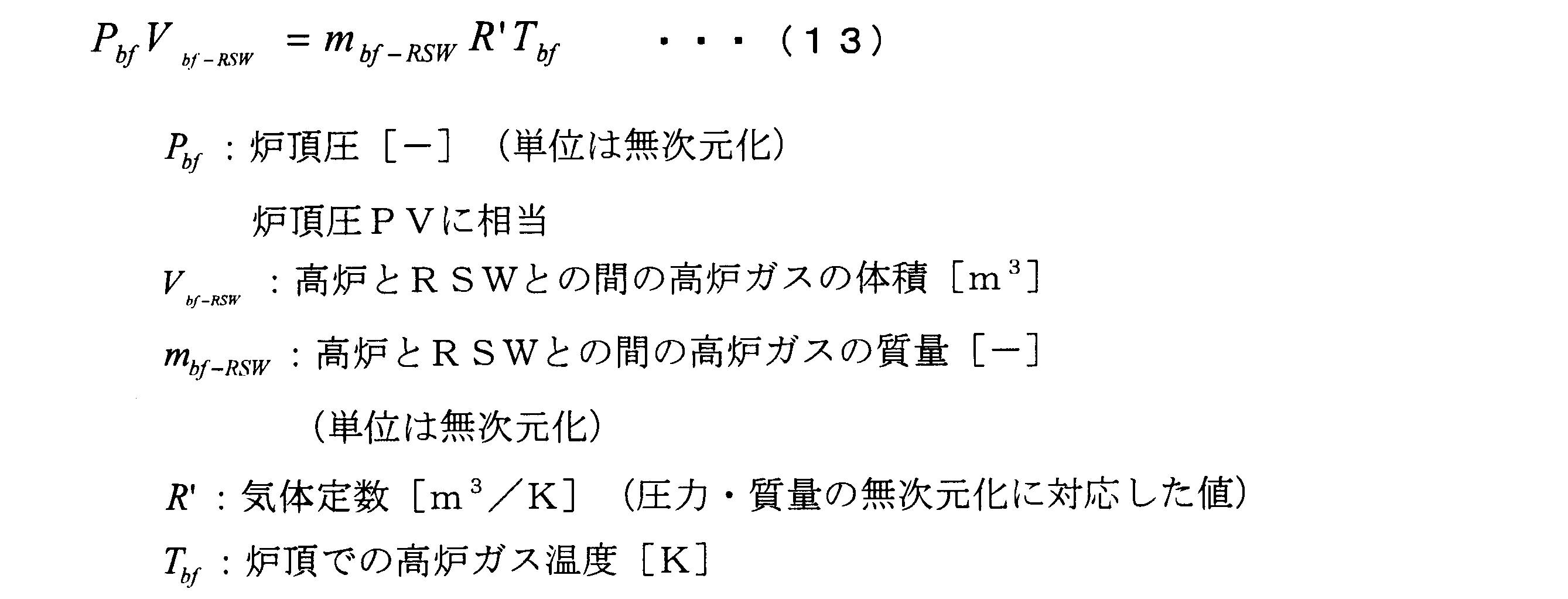
RSW-入口間の状態方程式は、次の通りである。なお、高炉ガスの質量は、「RSEでの高炉ガス流量-TRTでの高炉ガス流量-第1バイパス弁での高炉ガス流量-第2バイパス弁での高炉ガス流量」を時間積分して求める。

炉頂圧コントローラ7、TRT前圧コントローラ8、バイパス弁前圧コントローラ9に関しては、PIDコントローラを採用しており、このコントローラ部分の制御モデルは次の通りである。なお、ゲインは既知とする。

式(15)においては、炉頂圧コントローラ7からの出力が、炉頂圧MV、あるいは、RSE2の開度に相当する。

式(16)においては、TRT前圧コントローラ8からの出力が、TRT前圧MV、あるいは、翼弁開度に相当する。

式(17)においては、バイパス弁前圧コントローラ9からの出力が、バイパス弁前圧MV、あるいは、バイパス弁開度に相当する。
なお、炉頂圧SVは炉頂圧目標値であり、前圧SVは前圧目標値である。
一方、RSE公称流量特性として、図11に示す公称CV値を用いる。なお、RSE2では、図11の縦軸のCV値は流量[1/s]そのものを指すものとする。なお、流量は、標準状態での流量、または、質量の流量としているが、前述のように質量は無次元化している。炉頂圧MVを入力すれば、RSE2の流量が出力される。
なお、炉頂圧SVは炉頂圧目標値であり、前圧SVは前圧目標値である。
一方、RSE公称流量特性として、図11に示す公称CV値を用いる。なお、RSE2では、図11の縦軸のCV値は流量[1/s]そのものを指すものとする。なお、流量は、標準状態での流量、または、質量の流量としているが、前述のように質量は無次元化している。炉頂圧MVを入力すれば、RSE2の流量が出力される。
TRT公称流量特性として、図9に示す公称CV値を用いる。TRT前圧MVを入力し、CV値を求め、このCV値と式(10)とから、TRT3の流量が出力される。
第2バイパス弁流量特性として、図10に示す公称CV値を用いる。バイパス弁前圧MVを入力し、CV値を求め、このCV値と式(11)とから、第2バイパス弁6bの流量が出力される。
第2バイパス弁流量特性として、図10に示す公称CV値を用いる。バイパス弁前圧MVを入力し、CV値を求め、このCV値と式(11)とから、第2バイパス弁6bの流量が出力される。
第1バイパス弁流量特性として、図10に示す公称CV値を用いる。FF補償量を入力し、CV値を求め、このCV値と式(11)とから、第1バイパス弁6aの流量が出力される。
なお、公称流量は、既知の公称高炉ガス流量である。この公称流量は、高炉ガス流量の定常値とし、一定の値とする。この定常値に対して、原料装入時等に外乱が印加することとなる。
なお、公称流量は、既知の公称高炉ガス流量である。この公称流量は、高炉ガス流量の定常値とし、一定の値とする。この定常値に対して、原料装入時等に外乱が印加することとなる。
ところで、本具体例のフィルタは、図17に示すような低周波域でゲインが大きく、高周波域でゲインが小さくなるようなフィルタを採用している。このフィルタは、外乱が存在する高周波域で、ゲインを小さくするようにしている。本例では、時定数100[s]の一次遅れのフィルタとしている。折点周波数は、1.59×10⁻³[Hz](周期628[s])である。
このように、推定すべき外乱に上記のフィルタを適用することで、フィルタ適用後の信号で高周波外乱が小さくなり、その小さくなった高周波外乱は後述の評価関数で評価されないこととなる。
すなわち、上記のフィルタを用いることで、最適化の際に、フィルタ適用前の高周波外乱の値は大きくなることができ、推定可能となる。
すなわち、上記のフィルタを用いることで、最適化の際に、フィルタ適用前の高周波外乱の値は大きくなることができ、推定可能となる。
なお、フィルタ適用後においても、低周波外乱の信号は減衰しないので、後述の評価関数で評価されることとなり、フィルタ適用前の低周波外乱の値は、最適化により小さな値となる。
以上をまとめると、外乱として、主に高周波域の外乱が、大きな値として推定されることとなる。
以上をまとめると、外乱として、主に高周波域の外乱が、大きな値として推定されることとなる。
一方、KCR,KCB2,KR,KT,KBは、推定されるべき、制御モデルのパラメータである。
なお、KCR,KCB2は、PIDコントローラ7,9に未知のゲインがある場合を想定している。また、KR,KT,KBは、RSE2、TRT3、バイパス弁6a,6bの特性に補正係数が必要な場合を想定している。
なお、KCR,KCB2は、PIDコントローラ7,9に未知のゲインがある場合を想定している。また、KR,KT,KBは、RSE2、TRT3、バイパス弁6a,6bの特性に補正係数が必要な場合を想定している。
ここで、高炉ガス流量外乱は、主に、鉄鉱石やコークスを高炉17に投入(装入)する際に、高炉ガス流量が減少するという変動を示した外乱である。なお、高炉ガス流量外乱には、高炉17内のガスの流れの乱れ等により、高炉ガス流量が変化することも含まれる。
図4に示すように、高炉ガス流量外乱を、時系列の各時刻の値に対応したカウントでの値を変数とする。
図4に示すように、高炉ガス流量外乱を、時系列の各時刻の値に対応したカウントでの値を変数とする。
制御モデル内のパラメータの評価関数としては、次の式(18)を用いた。
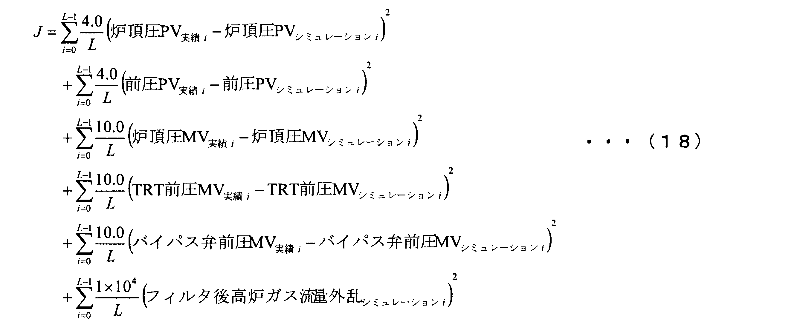
ここで、式(18)において、添え字の「実績」は既に得られている実績値を意味し、「シミュレーション」は、シミュレーション値を意味する。
式(18)の第1項~第5項は、yiについて、シミュレーション値を実績値に一致させるための項であり、具体的には、制御量(PV)と、操作量(MV)を、実績とシミュレーションで一致させるための項である。なお、式(18)の第6項は、フィルタ適用後の外乱を、0(ゼロ)に近づけるための項である。
式(18)の第1項~第5項は、yiについて、シミュレーション値を実績値に一致させるための項であり、具体的には、制御量(PV)と、操作量(MV)を、実績とシミュレーションで一致させるための項である。なお、式(18)の第6項は、フィルタ適用後の外乱を、0(ゼロ)に近づけるための項である。
制約条件については、次の通りであり、式(7)に対応する。

なお、各制約条件については、パラメータの取り得る値を考慮して、広めに設定している。
以上をまとめると、本具体例における炉頂圧制御は、一般形を具体化した形となっている。
次に、本具体例における炉頂圧制御について、具体的に説明する。
以上をまとめると、本具体例における炉頂圧制御は、一般形を具体化した形となっている。
次に、本具体例における炉頂圧制御について、具体的に説明する。
xi(状態量)の成分は、高炉-RSW間の高炉ガスの質量と、RSW-入口間の高炉ガスの質量とを求めるための2つの積分器、各PIDコントローラ7~9の積分器を離散化した場合の状態量となる。例えば、[1/s=サンプリング時間/(1-z-1)]と離散化した場合には、mx=5であるが、離散化方法により異なる。なお、L=101とした。
x0(初期値)については、この実施例では、変数とせず、固定値とする。炉頂とRSWとの間の高炉ガスの質量の初期値、及びRSWとTRT3とバイパス弁6a,6bとの間の高炉ガスの質量の初期値は、時刻が0のときの、圧力、体積、温度が既知であるため、状態方程式から得られる計算値とする。
また、各PIDコントローラ7~9のIゲインの積分器の初期値は、時刻が0のときの操作量(MV)が得られているため、Pゲイン、Dゲインを近似的に無視すると、操作量(MV)から逆算できるため、この値を採用する。例えば、「Iゲイン×積分器=操作量(MV)」であり、Iゲイン、積分器の順に掛け算がなされて操作量(MV)が得られる場合には、その得られた操作量(MV)が初期値となる。
また、各PIDコントローラ7~9のIゲインの積分器の初期値は、時刻が0のときの操作量(MV)が得られているため、Pゲイン、Dゲインを近似的に無視すると、操作量(MV)から逆算できるため、この値を採用する。例えば、「Iゲイン×積分器=操作量(MV)」であり、Iゲイン、積分器の順に掛け算がなされて操作量(MV)が得られる場合には、その得られた操作量(MV)が初期値となる。
ri(既知の入力)の成分は、公称高炉ガス流量、炉頂圧の目標値(SV)、前圧の目標値(SV)、温度を用いる箇所での高炉ガス温度、TRT3・バイパス弁6a,6bの背圧、(従来制御での)FF補償量とする。この場合、mr=6である。
dj(未知の入力)は、推定すべき外乱であり、公称高炉ガス流量に印加する、高炉ガス流量外乱である。この場合、md=1である。なお、M=41とした。
dj(未知の入力)は、推定すべき外乱であり、公称高炉ガス流量に印加する、高炉ガス流量外乱である。この場合、md=1である。なお、M=41とした。
p(推定すべきパラメータ)は、図16中のKCR,KCB2,KR,KT,KBである。この場合、mp=5である。
yi(一致すべき変数)の成分は、炉頂圧の制御量(PV)と、前圧の制御量(PV)、炉頂圧の操作量(MV)、TRT前圧の操作量(MV)、バイパス弁前圧の操作量(MV)としている。my=5である。
yi(一致すべき変数)の成分は、炉頂圧の制御量(PV)と、前圧の制御量(PV)、炉頂圧の操作量(MV)、TRT前圧の操作量(MV)、バイパス弁前圧の操作量(MV)としている。my=5である。
ddi(外乱にフィルタや積分等の操作を行った後の値)は、上記の高炉ガス流量外乱にフィルタを適用した後のフィルタ後高炉ガス流量外乱である。上述のように、md=1である。
fd()は、離散系において、状態量を計算する制御モデルであり、図16に示すモデルが離散化されたモデルである。ここでは、公用ソフトウェアであるThe MathWorks,Inc.製のSimulink(Simulinkは、The MathWorks,Inc.の登録商標)を用いて、離散化と計算を行っている。
fd()は、離散系において、状態量を計算する制御モデルであり、図16に示すモデルが離散化されたモデルである。ここでは、公用ソフトウェアであるThe MathWorks,Inc.製のSimulink(Simulinkは、The MathWorks,Inc.の登録商標)を用いて、離散化と計算を行っている。
なお、離散系の方程式は、固定サンプリング周期で解くことを前提として説明しているが、上記ソフトウェアで可能なように、サンプリング周期は可変でもよい。また、モデル内の積分器は、上記ソフトウェアでは、離散化されて計算されることとなる。
cdineq()は、不等式制約式であり、上記の式(19)である(mcdineq=92)。
cdeq()は、等式制約式であるが、本具体例では用いていない(mcdeq=0)。
cdineq()は、不等式制約式であり、上記の式(19)である(mcdineq=92)。
cdeq()は、等式制約式であるが、本具体例では用いていない(mcdeq=0)。
評価関数の重みは、それぞれ、以下の式(20)、式(21)のようになる。

図3のフローチャートに基づき、最適化の結果、次のパラメータを得た。ここで、第1バイパス弁6aのフィードフォワード量は実績値を用いている。また、翼弁開度は、トリップ後に実績と同じ値の0(ゼロ)としている。さらに、トリップ後には、TRT3を流れる流量が0となるようにTRT3の前の遮断弁が閉じられるので、TRT3を流れる流量を0としている。

また、このときの高炉ガス流量外乱は、図18Fに示すグラフ(太破線)のように、推定される。外乱の定常偏差はほぼ0(ゼロ)であり、周期が約20秒の高周波域の外乱が推定されていることがわかる。なお、図18A~E、図18Gの各グラフに、他の実績データ(実線)とシミュレーション結果のデータ(破線)を示す。
このように、式(22)に基づいて、CV値を補正し、精確なフィードフォワード補償量を得ることができる。
このように、式(22)に基づいて、CV値を補正し、精確なフィードフォワード補償量を得ることができる。
図19に、精確なフィードフォワード補償を適用した場合のシミュレーション結果のデータを示す。ここで、図19Fのグラフ(太破線)に示すように、外乱として、既に推定されたものをシミュレーションに使用する。また、既に推定されたパラメータを使用する。
なお、図19A~E、図19Gの各グラフに、他の実績データ(実線)とシミュレーション結果のデータ(破線)を示す。図19Aの炉頂圧の制御量(PV)の実績データ、及びシミュレーション結果のデータを示すグラフを参照すると、目標の炉頂圧が1.325[-]であるので、炉頂圧変動が、図18A中の0.036から、図19A中の0.011へと低減されていることがわかる。
なお、図19A~E、図19Gの各グラフに、他の実績データ(実線)とシミュレーション結果のデータ(破線)を示す。図19Aの炉頂圧の制御量(PV)の実績データ、及びシミュレーション結果のデータを示すグラフを参照すると、目標の炉頂圧が1.325[-]であるので、炉頂圧変動が、図18A中の0.036から、図19A中の0.011へと低減されていることがわかる。
なお、他に、上記した同時推定方法を用いて、PIDコントローラ7~9のゲイン調整等に使用することができる。例えば、外乱の影響を受ける操作量(MV)の大きさや速度について、飽和しないようなゲインを選ぶことができる。また、推定された外乱を、設備診断等に用いることもできる。さらに、H∞制御やオブザーバ等のコントローラ設計に用いることができる。
以上述べた具体例では、制御系を切り換えるという非定常時のデータを用いて、パラメータと外乱を同時に推定したが、制御系の切り換えを伴わない非定常時の場合でも推定ができることを、変形例として以下に示す。
[変形例]
図20に、第1バイパス弁6aを閉じたまま、第2バイパス弁6bを徐々に閉めていく場合の例の結果を示す。図20Fのグラフ(太破線)には、推定された外乱が示されている。外乱の定常偏差はほぼ0(ゼロ)であり、また、周期が約40秒の高周波域の外乱が推定されていることがわかる。なお、図20A~E、図20Gの各グラフには、他の実績値(実線)とシミュレーション結果(破線)が示されている。
[変形例]
図20に、第1バイパス弁6aを閉じたまま、第2バイパス弁6bを徐々に閉めていく場合の例の結果を示す。図20Fのグラフ(太破線)には、推定された外乱が示されている。外乱の定常偏差はほぼ0(ゼロ)であり、また、周期が約40秒の高周波域の外乱が推定されていることがわかる。なお、図20A~E、図20Gの各グラフには、他の実績値(実線)とシミュレーション結果(破線)が示されている。
ここで、評価関数と不等式制約条件は、式(18)、(19)と同じである。
なお、第2バイパス弁6bの操作量(MV)には、実績値を与えているため、KCB2は、推定すべきパラメータに含まれない。このことから、KCB2をcdeq()(等式制約式)で次のように設定しておけばよい。
なお、第2バイパス弁6bの操作量(MV)には、実績値を与えているため、KCB2は、推定すべきパラメータに含まれない。このことから、KCB2をcdeq()(等式制約式)で次のように設定しておけばよい。

そして、図3のフローチャート図に基づき、最適化を行う。その結果、以下に示す式(24)のようなパラメータを得た。ここで、なお、第1バイパス弁6a、第2バイパス弁6bの開度は、実績値をそのまま用いている。

このように、操業条件に合わせて、シミュレーション条件を変え、また、推定すべきパラメータを変更することで、パラメータや外乱を適切に推定することができる。
[2例目]
続いて、具体例の2例目について、説明する。2例目は、鉄鋼プロセスの1つである連続鋳造機30の鋳型31内にある溶鋼Xの湯面レベルを制御する方法について、外乱とパラメータとを同時推定し、制御偏差が生じる原因を特定し、さらに、制御系を調整する方法について説明する。
[2例目]
続いて、具体例の2例目について、説明する。2例目は、鉄鋼プロセスの1つである連続鋳造機30の鋳型31内にある溶鋼Xの湯面レベルを制御する方法について、外乱とパラメータとを同時推定し、制御偏差が生じる原因を特定し、さらに、制御系を調整する方法について説明する。
図21に示す如く、タンディッシュ33の底部には、タンディッシュ33内の溶鋼Xを鋳型31へ排出する溶鋼孔34が形成されている。この溶鋼孔34に連通するように浸漬ノズル35が設けられ、浸漬ノズル35の先端部は鋳型31内に挿入されるものとなっている。タンディッシュ33の底部であって、浸漬ノズル35の根本には、溶鋼孔34に隣接するように、浸漬ノズル35内を流下する溶鋼Xの流量を調整するスライドバルブ36が設けられている。
スライドバルブ36は、定形耐火物で構成された固定の板状の上プレート36a、下プレート36bと、定形耐火物で構成された移動する板状の中間プレート36cとを有している。 上プレート36aの下面と中間プレート36cの上面とは面接触していて、中間プレート36cの上面は、上プレート36aの下面を水平方向に摺動するようになっている。なお、下プレート36bと中間プレート36cとの関係は、上下の位置関係が異なる点を除いて、上プレート36aと中間プレート36cとの関係と同じである。上プレート36a、下プレート36bと中間プレート36cとには、上下に貫通していてタンディッシュ33から排出された溶鋼Xを通す流下孔37(バルブ)が設けられている。
中間プレート36cは、ロッドが水平方向に伸縮する電気油圧シリンダ39(アクチュエータ)に連結されていて、この電気油圧シリンダ39のロッドを伸縮させることで、中間プレート36cは、上プレート36aと下プレート36bとの間を水平方向に摺動し、流下孔37の断面積(バルブ断面積)が変化し、流下する溶鋼Xの流量が可変とされる。さらに、図21に示す如く、鋳型31の上方には、鋳型31内の湯面レベルを計測する湯面レベル計38が設けられている。なお、湯面レベルとは、鋳型31内の溶鋼表面(湯面)の高さのことをいう。加えて、この湯面レベル計38の計測結果などを基に、鋳型31内の湯面レベルを目標値に一致させるべく、スライドバルブ36の位置、言い換えれば電気油圧シリンダ39の伸縮量を算出し、算出された量をスライドバルブ36へ適用する制御部40(コントローラ)が、連続鋳造機30には備えられている。
図22は、制御部40で行われる鋳型31内の湯面レベル制御系(単に、レベル制御系と呼ぶこともある)のブロック図を示したものである。
図22において、CFB(z)がフィードバックコントローラであり、遅延要素z-1の関数である。なお、遅延要素がない場合(動特性がない場合)も含むものとする。アクチュエータ39や湯面レベル計38は、それぞれ「一次遅れ+むだ時間」で表され、シミュレーション時には、離散化される。
図22において、CFB(z)がフィードバックコントローラであり、遅延要素z-1の関数である。なお、遅延要素がない場合(動特性がない場合)も含むものとする。アクチュエータ39や湯面レベル計38は、それぞれ「一次遅れ+むだ時間」で表され、シミュレーション時には、離散化される。
シミュレーションには、既述のように、公用ソフトウェアであるThe MathWorks,Inc.製のSimulink(Simulinkは、The MathWorks,Inc.の登録商標)を用いることができる。スライドバルブ36は、流量係数Kfのゲインで表される。鋳型31は、鋳型断面積Amoldの逆数をゲインとする積分器で表される。
図23に、湯面レベルが定常偏差を持ってハンチングしている異常状態の一例を示す。
図23に、湯面レベルが定常偏差を持ってハンチングしている異常状態の一例を示す。
スライドバルブ開度のグラフ(実線)は、実績値を示す。湯面レベルのグラフは、実線が実績値(湯面レベル制御のPV)を示し、一点鎖線が、目標値(湯面レベル制御のSV)を示す。
時刻0~約50秒の間は、コントローラA(40)が制御している。時刻約50~160秒の間は、コントローラB(40)が制御している。湯面レベルのグラフを見てわかるように、周期が約40秒のハンチングを生じている。さらに、湯面レベル目標値(湯面レベルSV)が、-1.02[-](一点鎖線)であるのに対して([-]は無次元化した値であることを示す。)、湯面レベル実績値は、約-0.95[-]を中心に振動しており、レベル偏差にオフセットを生じている。これらのハンチングと定常偏差が制御上の問題である。
時刻0~約50秒の間は、コントローラA(40)が制御している。時刻約50~160秒の間は、コントローラB(40)が制御している。湯面レベルのグラフを見てわかるように、周期が約40秒のハンチングを生じている。さらに、湯面レベル目標値(湯面レベルSV)が、-1.02[-](一点鎖線)であるのに対して([-]は無次元化した値であることを示す。)、湯面レベル実績値は、約-0.95[-]を中心に振動しており、レベル偏差にオフセットを生じている。これらのハンチングと定常偏差が制御上の問題である。
ハンチングと定常偏差の原因の候補として、外乱(例えば、バルジング等による外乱)、制御によるハンチング(例えば、制御ゲインが高すぎる、時定数が長すぎる、むだ時間が長すぎる、把握していない制御ゲインがループ内に存在する等)、ハードウェアの異常動作(想定外の動作)等が挙げられる。しかし、外乱と制御系パラメータの両方が不明であるため、異常原因の特定が困難であった。
そこで、制御モデルのパラメータと、その制御モデルに加わる外乱の推定により、このレベル制御異常の原因を特定することとした。
図24に、連続鋳造機30の湯面レベル制御系の制御モデルと外乱を示す。
図24中のフィルタsは、図25に示すようなバンドストップフィルタとしている。具体的には、(s2+ωb 2)/(s2+2ζbωbs+ωb 2),ωb=2π/13.5,ζb=0.8としている。すなわち、湯面レベル外乱の周期は、13.5秒近傍としている。湯面レベルの外乱の主な成分は、バルジングと呼ばれる凝固殻が、鋳型31下方のロール32の間で膨らんだり凹んだりすることで、鋳型31の湯面高さが変わることによる外乱(バルジング外乱)であり、この外乱の周波数は、鋳造速度/ロール32間隔である。
図24に、連続鋳造機30の湯面レベル制御系の制御モデルと外乱を示す。
図24中のフィルタsは、図25に示すようなバンドストップフィルタとしている。具体的には、(s2+ωb 2)/(s2+2ζbωbs+ωb 2),ωb=2π/13.5,ζb=0.8としている。すなわち、湯面レベル外乱の周期は、13.5秒近傍としている。湯面レベルの外乱の主な成分は、バルジングと呼ばれる凝固殻が、鋳型31下方のロール32の間で膨らんだり凹んだりすることで、鋳型31の湯面高さが変わることによる外乱(バルジング外乱)であり、この外乱の周波数は、鋳造速度/ロール32間隔である。
ロール32間隔が一定でない場合は、バルジングを生じる部分のロール32間隔の最大・最小から、周波数の最小・最大を求め、この最小・最大の間の周波数の信号をストップするようなフィルタとすればよい。
図24中のフィルタcは、図26に示すように、コントローラ40に加わる外乱の微分値(コントローラ外乱の微分値)に適用するフィルタである。フィルタの形は、図25と同じとしている。外乱の微分値に周期が13.5秒近傍の成分が含まれていると予想して推定することとなる。なお、後述のように、結果として、この周期のコントローラ外乱は存在しないと推定された。すなわち、周期13.5秒近傍の外乱は、湯面レベル外乱であることが確認された。コントローラ40に加わる外乱は、図27に示すように、積分され、ランプ状の外乱を表現することができる。
図24中のフィルタcは、図26に示すように、コントローラ40に加わる外乱の微分値(コントローラ外乱の微分値)に適用するフィルタである。フィルタの形は、図25と同じとしている。外乱の微分値に周期が13.5秒近傍の成分が含まれていると予想して推定することとなる。なお、後述のように、結果として、この周期のコントローラ外乱は存在しないと推定された。すなわち、周期13.5秒近傍の外乱は、湯面レベル外乱であることが確認された。コントローラ40に加わる外乱は、図27に示すように、積分され、ランプ状の外乱を表現することができる。
続いて、本具体例の制御モデルについて、説明する。
コントローラA,B(40)は、k=0,1に対応する。ここで、コントローラA(40)で制御している場合と、コントローラB(40)で制御している場合を、それぞれ別のデータとして切出すこととする。すなわち、実績データの時系列値が複数群存在する場合である。この例では、2つの群が存在することとなる。コントローラA,B(40)は、次の式で表される。
コントローラA,B(40)は、k=0,1に対応する。ここで、コントローラA(40)で制御している場合と、コントローラB(40)で制御している場合を、それぞれ別のデータとして切出すこととする。すなわち、実績データの時系列値が複数群存在する場合である。この例では、2つの群が存在することとなる。コントローラA,B(40)は、次の式で表される。

なお、z-1は、既述のように、サンプリング周期の時間の遅延要素を意味している。また、z-nodは、nodサンプリング周期分の時間の遅延要素を意味している。
ここで、各係数は既知であり、次の値としている。
ここで、各係数は既知であり、次の値としている。

各kの場合に、分母分子のそれぞれの遅延要素の初期値として、式(25)の分子のz-1,z-2,z-3,z-4にそれぞれ、u1init_k,u2init_k,u3init_k,u4init_k(k=0,1)を代入し、式(25)の分母のz-1,z-2,z-3,z-4にそれぞれ、y1init_k,y2init_k,y3init_k,y4init_k(k=0,1)を代入する。これにより、コントローラ40の出力の初期値を計算することができる。
コントローラ40の未知のゲインを、kconとする。例えば、コントローラ40の仕様が明確でない場合等を想定している。
制御対象のゲインである流量係数/鋳型断面積は、次のように決定した。
制御対象のゲインである流量係数/鋳型断面積は、次のように決定した。

次の積分器は、1/sで表され、出力の初期値をlevelinit_k(k=0,1)とする。
次の一次遅れは、制御対象の一次遅れ成分を意味し、一次遅れ「1/(Tlag・s+1)」で表され、時定数Tlagがパラメータであり、状態量を1つ含んでいるため、出力の初期値をlevellaginit_k(k=0,1)とする。
次の一次遅れは、制御対象の一次遅れ成分を意味し、一次遅れ「1/(Tlag・s+1)」で表され、時定数Tlagがパラメータであり、状態量を1つ含んでいるため、出力の初期値をlevellaginit_k(k=0,1)とする。
この制御モデルでは、アクチュエータ39の時定数は小さいとして無視し、湯面レベル真値と湯面レベル観測値との間に一次遅れがあるものとしている。この一次遅れには、センサの特性と、センサに追加されたフィルタの特性とを含むものとする。なお、シミュレーション時には、適宜、離散化され解かれることとなる。
次のむだ時間要素は、制御対象のむだ時間の成分を意味し、むだ時間Tdelay[s]前の値を現在の値とする要素である。シミュレーションの初期には、過去の値を初期値として与える必要があり、過去のTdelay[s]前までの初期値をleveldelayinit_k(k=0,1)とするものとする。
次のむだ時間要素は、制御対象のむだ時間の成分を意味し、むだ時間Tdelay[s]前の値を現在の値とする要素である。シミュレーションの初期には、過去の値を初期値として与える必要があり、過去のTdelay[s]前までの初期値をleveldelayinit_k(k=0,1)とするものとする。
この制御モデルでは、アクチュエータ39のむだ時間は小さいとして無視し、湯面レベル真値と湯面レベル観測値との間にむだ時間があるものとしている。このむだ時間には、センサの特性、フィルタの特性、制御のサンプリング周期の特性等を含むものとする。なお、シミュレーション時には、適宜、離散化され解かれることとなる。
ゲインkplantは、制御対象の未知のゲインを示し、本具体例では、流量係数Kfの変動分や他の動特性による変動分を合わせた制御対象全体の未知ゲインを表す。kplantは、制御モデルと一致していれば1である。
ゲインkplantは、制御対象の未知のゲインを示し、本具体例では、流量係数Kfの変動分や他の動特性による変動分を合わせた制御対象全体の未知ゲインを表す。kplantは、制御モデルと一致していれば1である。
開度定常値MVsteady_k(k=0,1)は、バルブ開度の定常値である。式(25)から得られる操作量(MV)は、偏差系に対する操作量で、0(ゼロ)が基準になるため、初期の状態での定常値を加えた値が、シミュレーションで得られるスライドバルブ開度となる。
本具体例では、図24などに示されている「湯面レベル目標値」、「湯面レベル」、「バルブ開度」が、それぞれ、レベル制御系の「湯面レベルSV」、「湯面レベルPV」、「湯面レベルMV」となる。
本具体例では、図24などに示されている「湯面レベル目標値」、「湯面レベル」、「バルブ開度」が、それぞれ、レベル制御系の「湯面レベルSV」、「湯面レベルPV」、「湯面レベルMV」となる。
以上より、推定すべきパラメータは、u1init_k,u2init_k,u3init_k,u4init_k,y1init_k,y2init_k ,y3init_k,y4init_k(k=0,1),kcon,levelinit_k(k=0,1),Tlag,levellaginit_k(k=0,1),Tdelay,leveldelayinit_k(k=0,1),kplant,MVsteady_k(k=0,1)となる。
この中で、kcon,Tlag,Tdelay,kplantが、共通パラメータであり、残りが個別のパラメータとなる。ここで、共通パラメータとは、複数の実績データを用いるときに、モデル内で共通の値として用いられるパラメータである。すなわち、実績データのすべての群にて共通する値をもつパラメータである。個別のパラメータとは、複数の実績データを用いるときに、モデル内で個別の値として用いられるパラメータである。すなわち、実績データの各群に連動する値をもつパラメータである。
この中で、kcon,Tlag,Tdelay,kplantが、共通パラメータであり、残りが個別のパラメータとなる。ここで、共通パラメータとは、複数の実績データを用いるときに、モデル内で共通の値として用いられるパラメータである。すなわち、実績データのすべての群にて共通する値をもつパラメータである。個別のパラメータとは、複数の実績データを用いるときに、モデル内で個別の値として用いられるパラメータである。すなわち、実績データの各群に連動する値をもつパラメータである。
また、u1init_k,u2init_k,u3init_k,u4init_k,y1init_k,y2init_k,y3init_k,y4init_k(k=0,1),levelinit_k(k=0,1),levellaginit_k(k=0,1),leveldelayinit_k(k=0,1),MVsteady_k(k=0,1)が、未知の初期値となる。ここで、未知の初期値とは、シミュレーションの初期に与えるべき値のうち、未知のものをいう。
さらに、MVsteady_k(k=0,1)は、未知の定常値である。未知の定常値とは、制御系として偏差系を構成し、シミュレーションをする際に与えるべき定常値のうち、未知のものをいう。
続いて、本具体例において、推定すべき外乱は、湯面レベルに加わる外乱と、スライドバルブ開度に加わるランプ状の外乱との2つである。
続いて、本具体例において、推定すべき外乱は、湯面レベルに加わる外乱と、スライドバルブ開度に加わるランプ状の外乱との2つである。
1つ目の湯面レベルに加わる外乱は、よく知られたバルジングに起因する外乱dlevel k j (k=0,1、j=0,…,Mk-1)であり、図4に示すように、時系列の各時刻の値に対応したカウントでの値を変数とする。この1つ目の外乱に、既述のように、フィルタsを適用した後のフィルタ後レベル外乱dlevelfilterd k j (k=0,1、j=0,…,Mk-1)を、後述のように評価する。
2つ目の外乱は、制御用のコンピュータが操作量(MV)を出力し、その後、実際にスライドバルブ開度の変化となるまでに印加する外乱である。
図23に示すように、2つ目の外乱は、湯面レベルが定常偏差を持っていることから、ランプ状の外乱であると推定されたものである。なお、この2つ目の外乱は、調査により、操作信号の伝達経路で信号が欠落することにより発生したことが後程確認された。
図23に示すように、2つ目の外乱は、湯面レベルが定常偏差を持っていることから、ランプ状の外乱であると推定されたものである。なお、この2つ目の外乱は、調査により、操作信号の伝達経路で信号が欠落することにより発生したことが後程確認された。
本具体例では、スライドバルブ開度に加わる外乱の微分値(コントローラ外乱の微分値)、d(ドット)MV k j(k=0,1、j=0,…,Mk-1)を推定することとしている。図4に示すように、外乱の微分値を、時系列の各時刻の値に対応したカウントでの値を変数とした。この外乱の微分値に、既述のように、フィルタcを適用した後のフィルタ後コントローラ外乱微分値d(ドット)MVfilterd k j(k=0,1、j=0,…,Mk-1)を、後述のように評価する。
なお、本具体例では、2つの実績データ、すなわち、コントローラA(40)で制御している場合の実績データと、コントローラB(40)で制御している場合の実績データとを用いているため、外乱は各実績データに対して別々であり且つ個別の外乱を用いている。個別の外乱とは、複数の実績データを用いてシミュレーションを行うときに、実績データ毎に個別の時系列の値として用いられる外乱である。すなわち、実績データの各群に連動する時系列変数値である。
本具体例の評価関数は、次のように定めた。すなわち、2つの実績データに対応するモデルで共通なパラメータは共通の変数とし、別々のパラメータは別の変数として推定することとしている。外乱については、別々なので、それぞれ別に推定することとなる。
そして、制御モデル内のパラメータの評価関数としては、次の式(28)を用いた。
そして、制御モデル内のパラメータの評価関数としては、次の式(28)を用いた。
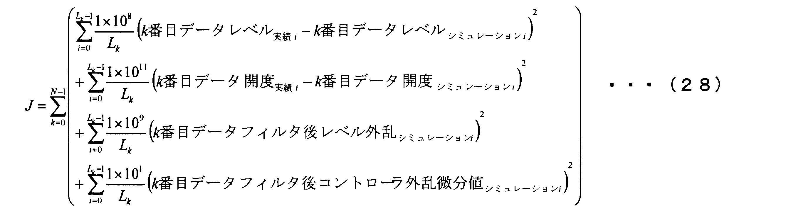
第1項、第2項は、湯面レベルとバルブ開度とを、実績とシミュレーションで一致させるための項である。第3項、第4項は、フィルタ後レベル外乱と、フィルタ後コントローラ外乱微分値とを0(ゼロ)に近づけるための項である。なお、N=2,L0=52,L1=101である。実績データと、シミュレーション結果のデータのサンプリング周期は、1秒である。
制御モデルの制約条件は、次の通りである。
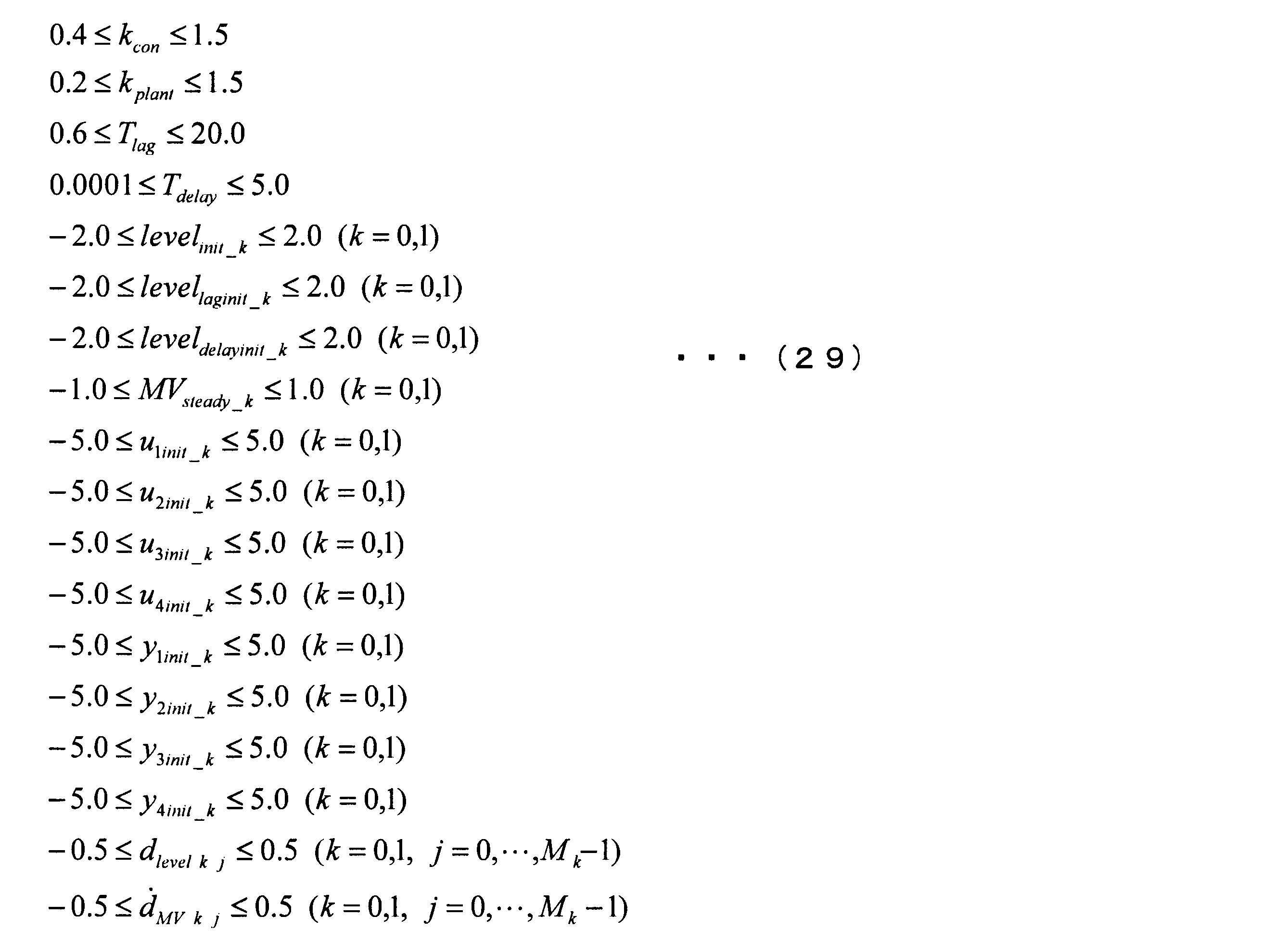
各制約条件については、パラメータの取り得る値を考慮して、広めに設定している。
以上をまとめると、本具体例における湯面レベル制御は、データ数が1つの場合を、データ数が複数の場合に拡張した一般形を、具体化した形となっている。
次に、本具体例における湯面レベル制御について、具体的に説明する。
xki(状態量)は、各k(k=0,1)について、コントローラ40の遅延要素の8個(分子4+分母4)、鋳型31の積分器1個に対応する遅延要素(離散化の方法に依存する)、一次遅れの積分器1個に対応する遅延要素(離散化の方法に依存する)、むだ時間要素の遅延要素(数は、離散化のサンプリング時間に依存する)、コントローラ外乱に対する積分器1個に対応する遅延要素である(状態量の数はシミュレーション方法に依存する。)。
以上をまとめると、本具体例における湯面レベル制御は、データ数が1つの場合を、データ数が複数の場合に拡張した一般形を、具体化した形となっている。
次に、本具体例における湯面レベル制御について、具体的に説明する。
xki(状態量)は、各k(k=0,1)について、コントローラ40の遅延要素の8個(分子4+分母4)、鋳型31の積分器1個に対応する遅延要素(離散化の方法に依存する)、一次遅れの積分器1個に対応する遅延要素(離散化の方法に依存する)、むだ時間要素の遅延要素(数は、離散化のサンプリング時間に依存する)、コントローラ外乱に対する積分器1個に対応する遅延要素である(状態量の数はシミュレーション方法に依存する。)。
x0k(初期値)は、コントローラ40の遅延要素の8個(分子4+分母4)の初期値、鋳型31の積分器に対応する遅延要素の初期値、一次遅れの積分器に対応する遅延要素の初期値、むだ時間要素の遅延要素の初期値である。なお、コントローラ外乱の微分値に適用する積分器に対応する遅延要素の初期値は0とした。
rki(既知の入力)は、各kに対応した湯面レベルSV(レベル目標値)である。
rki(既知の入力)は、各kに対応した湯面レベルSV(レベル目標値)である。
dkj(未知の入力)は、推定すべき外乱であり、コントローラ外乱の微分値と、レベル外乱との2つである(k毎にmdk=2)。
パラメータとしては、図4のように、時系列の各時刻の値を変数とし、M0=20,M1=40とした。外乱の変数の時間間隔が、実績データやシミュレーション結果のデータのサンプリング周期1秒より長いのは、外乱の変数を減らすことを可能とするためである。例えば、外乱の時間的変化が滑らかと予想される場合には、外乱の変数の時間間隔を長くとることができ、最適化のための計算量を減らすことができる。
パラメータとしては、図4のように、時系列の各時刻の値を変数とし、M0=20,M1=40とした。外乱の変数の時間間隔が、実績データやシミュレーション結果のデータのサンプリング周期1秒より長いのは、外乱の変数を減らすことを可能とするためである。例えば、外乱の時間的変化が滑らかと予想される場合には、外乱の変数の時間間隔を長くとることができ、最適化のための計算量を減らすことができる。
p(推定すべきパラメータ)は、既述のように、u1init_k,u2init_k,u3init_k,u4init_k,y1init_k,y2init_k,y3init_k,y4init_k(k=0,1),kcon,levelinit_k(k=0,1),Tlag,levellaginit_k(k=0,1),Tdelay,leveldelayinit_k(k=0,1),kplant,MVsteady_k(k=0,1)となる(mp=28)。
ykiは、一致すべき変数であり、湯面レベルPV(湯面レベル)、湯面レベルMV(バルブ開度)としている(k毎にmyk=2)。
ddkiは、外乱にフィルタや積分等の操作を行った後の値であり、コントローラ外乱の微分値にローパスフィルタを適用した後の値(フィルタ後コントローラ外乱微分値)と、レベル外乱にバンドストップフィルタを適用した後の値(フィルタ後レベル外乱)である。
ddkiは、外乱にフィルタや積分等の操作を行った後の値であり、コントローラ外乱の微分値にローパスフィルタを適用した後の値(フィルタ後コントローラ外乱微分値)と、レベル外乱にバンドストップフィルタを適用した後の値(フィルタ後レベル外乱)である。
fd()は、離散系において、状態量を計算する制御モデルであり、図24に示すモデルから離散化して得られる制御モデルである。本具体例では、公用ソフトウェアであるThe MathWorks,Inc.製のSimulink(Simulinkは、The MathWorks,Inc.の登録商標)を用いて行っている。
なお、本具体例の離散系の方程式は、固定サンプリング周期で解くことを前提として説明しているが、上記ソフトウェアで可能なように、サンプリング周期は可変でよい。また、制御モデル内の積分器は、上記ソフトウェアにおいて、離散化されて計算されることとなる。
なお、本具体例の離散系の方程式は、固定サンプリング周期で解くことを前提として説明しているが、上記ソフトウェアで可能なように、サンプリング周期は可変でよい。また、制御モデル内の積分器は、上記ソフトウェアにおいて、離散化されて計算されることとなる。
cdineq()は、不等式制約式であり、上記の式(29)である(mcdineq=296)。
cdeq()は、等式制約式であるが、本具体例では用いていない(mcdeq=0)。
制御モデル内のパラメータの評価関数は、式(9)を、複数の実績データに対応して、拡張した次の式(30)となる。
cdeq()は、等式制約式であるが、本具体例では用いていない(mcdeq=0)。
制御モデル内のパラメータの評価関数は、式(9)を、複数の実績データに対応して、拡張した次の式(30)となる。

ここで、各変数は次の通りである。
Nは、実績データの数である。
yactual k iは、k番目のデータの、myk行1列のベクトル(i=0,・・・,Lk-1)。各成分は、カウントiでの、時系列の実績データと、シミュレーション結果のデータとを一致させる場合の、実績データである。
Nは、実績データの数である。
yactual k iは、k番目のデータの、myk行1列のベクトル(i=0,・・・,Lk-1)。各成分は、カウントiでの、時系列の実績データと、シミュレーション結果のデータとを一致させる場合の、実績データである。
Wykは、myk行myk列の行列。シミュレーション結果のデータの重みを示す。本具体例では、対称な準正定行列とする。
Wddkは、mdk行mdk列の行列。外乱にフィルタや積分等の操作を行った後の値の重みを示す。本具体例では、対称な準正定行列とする。
具体的な数値は、次のようになる。
Wddkは、mdk行mdk列の行列。外乱にフィルタや積分等の操作を行った後の値の重みを示す。本具体例では、対称な準正定行列とする。
具体的な数値は、次のようになる。
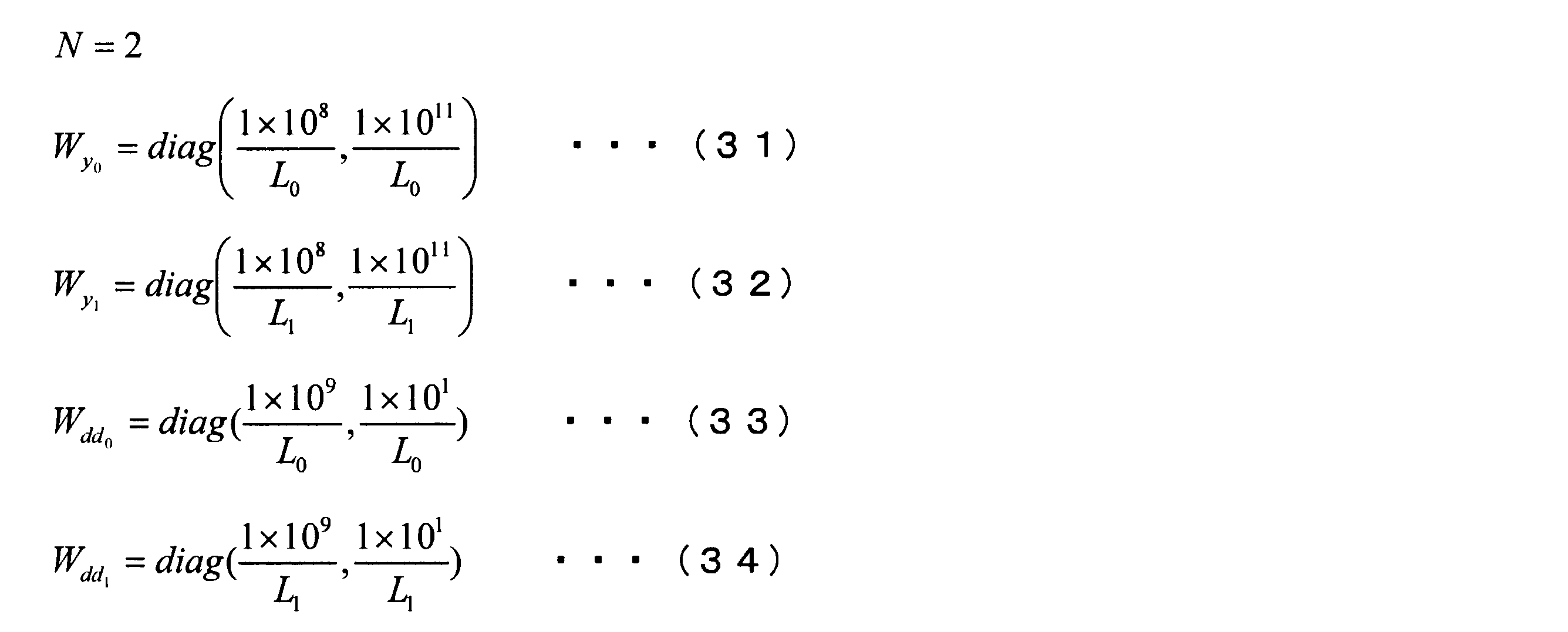
図28のフローチャート図に基づいた最適化計算を行い、その結果、以下に示すパラメータを得た。

また、このときの2つの実績データに対応する外乱は、図29E~図29Hのグラフ(太破線)のように推定される。なお、図29G、図29Hに示すコントローラ外乱については、積分した後の値を表示している。図29E、図29Fに示すように、推定されたレベル外乱が小さいことから、連続鋳造機30において、小さなバルジングが発生していることが推測される。バルジング外乱は、周期が約13.5秒と推定されている。また、湯面レベル外乱の定常偏差はほぼ0(ゼロ)と推定されている。また、コントローラ外乱として、ランプ状の外乱が印加されていることが推測される。細かくは、コントローラ外乱として、ランプ状の外乱と、重畳した周期約40秒の小さな外乱が印加していると推定されている。これらの周波数帯域の外乱は、外乱微分値が存在すると予想した周波数帯域外にあり、外乱微分値が小さな値として推定されていることとなる。なお、存在すると予想した周期約13.5秒近傍の外乱は、推定されておらず、周期13.5秒近傍の外乱は、コントローラ外乱ではなく、レベル外乱であると推測される。
ちなみに、外乱の時系列値を評価しない場合、すなわち、Wdd0,Wdd1が零行列の場合には、レベル外乱がランプ状であるような想定外の推定結果が得られた。したがって、外乱の時系列値を評価しない場合、外乱が大きくなる解がある場合には、外乱の大きさに制限を加えることが望ましい。すなわち、外乱の時系列値を評価する方が望ましい。
なお、図29A~図29Dは、実績データ(実線)とシミュレーション結果のデータ(破線)である。一点鎖線は、目標値を示している。
なお、図29A~図29Dは、実績データ(実線)とシミュレーション結果のデータ(破線)である。一点鎖線は、目標値を示している。
以上の推定結果から、制御コンピュータからスライドバルブ開度までの信号経路に異常があることが推測される。なお、既述のように、実際に異常が存在したことが確認されている。
また、周期約40秒の振動は、主に、制御対象の位相遅れによる制御起因であると推定される。
また、周期約40秒の振動は、主に、制御対象の位相遅れによる制御起因であると推定される。
そこで、信号経路上の異常に対策を実施し、制御対象の位相遅れを除く処理を行った。
その結果、図30に示すように、この周期約40秒の大きな振動はなくなり、レベル精
度を向上させることができた。
なお、制御モデル内のパラメータと、その制御モデルに加わる外乱が得られているので、従来のPID制御を適用する場合に、ゲイン調整を行い、制御することも、既述のように可能である。
[3例目]
さて、具体例の3例目について、3つ例を挙げて説明する。この3例目は、評価関数に外乱の時系列変数値を含まない例である。
(3例目の1)
まず、3例目の1は、図31に示すように、ゲインK、時定数Tの一次遅れ、むだ時間Lで構成された制御対象である。なお、コントローラとしてPI制御が使用され、比例ゲインをKP、積分ゲインをKIとする。また、一次遅れの初期値をlaginit_tv、むだ時間の初期値をdelayinit_tv、コントローラの積分要素の初期値をIinit_tvとする。また、連続系の要素は、シミュレーション時に離散化されることとなる。また、外乱をd(t)とおく。
その結果、図30に示すように、この周期約40秒の大きな振動はなくなり、レベル精
度を向上させることができた。
なお、制御モデル内のパラメータと、その制御モデルに加わる外乱が得られているので、従来のPID制御を適用する場合に、ゲイン調整を行い、制御することも、既述のように可能である。
[3例目]
さて、具体例の3例目について、3つ例を挙げて説明する。この3例目は、評価関数に外乱の時系列変数値を含まない例である。
(3例目の1)
まず、3例目の1は、図31に示すように、ゲインK、時定数Tの一次遅れ、むだ時間Lで構成された制御対象である。なお、コントローラとしてPI制御が使用され、比例ゲインをKP、積分ゲインをKIとする。また、一次遅れの初期値をlaginit_tv、むだ時間の初期値をdelayinit_tv、コントローラの積分要素の初期値をIinit_tvとする。また、連続系の要素は、シミュレーション時に離散化されることとなる。また、外乱をd(t)とおく。
次の式(36)のように、制御モデルのパラメータと、外乱の真値を決定する。なお、_tvは、真値を示す添え字である。

図32A~Dに、真値のパラメータと、真値の外乱の場合の実績データを示す。なお、ここでは、真値、または、真値を用いたシミュレーション結果を、実績データとしている。本具体例では、この実績データから、制御モデルのパラメータと外乱とを逆算することを考えている。なお、実績データの外乱は、ランプ状外乱やオフセットを含んでいることとしている。
評価関数としては、次の式(37)を用いた。

ここでは、式(37)において、添え字の「実績」は、既に得られている実績値を意味し、「シミュレーション」は、シミュレーション値を意味する。
また、式(37)の第1項~第2項は、yiについて、シミュレーション値を実績値に一致させるための項であり、具体的には、制御量(PV)と、操作量(MV)を、実績とシミュレーションで一致させるための項である。
また、式(37)の第1項~第2項は、yiについて、シミュレーション値を実績値に一致させるための項であり、具体的には、制御量(PV)と、操作量(MV)を、実績とシミュレーションで一致させるための項である。
なお、式(37)では、外乱を評価していない。式(9)で、Wdd=0とした場合に相当し、評価関数が外乱の時系列変数値を含まないこととなる。
制約条件については、次の式(38)の通りであり、式(7)に対応する。
制約条件については、次の式(38)の通りであり、式(7)に対応する。
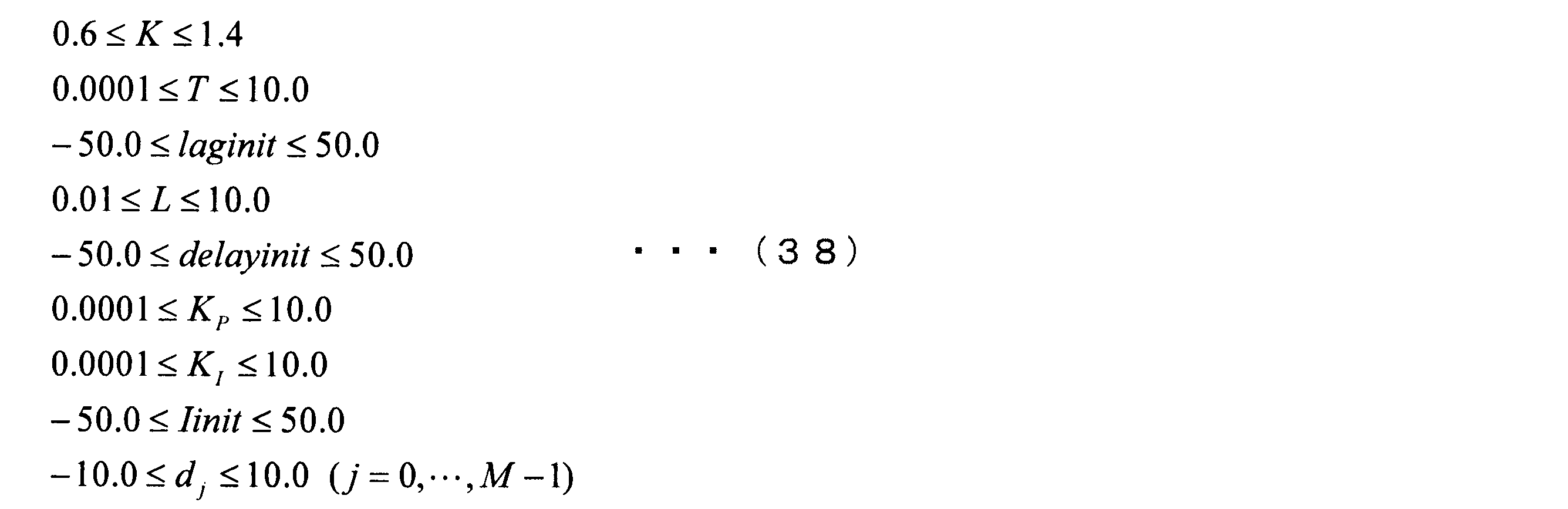
なお、各制約条件については、パラメータの取り得る値を考慮して、広めに設定している。
以上をまとめると、本具体例は、一般形を具体化した形となっている。以下に、本具体例の詳細を説明する。
xi(状態量)の成分は、まず、時定数の積分器、PIDコントローラの積分器を離散化した場合の状態量である。さらに、むだ時間を離散化した場合の状態量、例えば、むだ時間1秒をサンプリング時間0.1秒で離散化した場合には過去の10点の10個の状態量がある。mxは、離散化方法やむだ時間により異なることとなる。なお、L=51とした。
以上をまとめると、本具体例は、一般形を具体化した形となっている。以下に、本具体例の詳細を説明する。
xi(状態量)の成分は、まず、時定数の積分器、PIDコントローラの積分器を離散化した場合の状態量である。さらに、むだ時間を離散化した場合の状態量、例えば、むだ時間1秒をサンプリング時間0.1秒で離散化した場合には過去の10点の10個の状態量がある。mxは、離散化方法やむだ時間により異なることとなる。なお、L=51とした。
x0(初期値)については、時定数の積分器とPIDコントローラの積分器を離散化した場合の状態量の初期値、むだ時間を離散化した場合の状態量の初期値である。
ri(既知の入力)の成分は、目標値(SV)である。この場合、mr=1である。
dj(未知の入力)は、推定すべき外乱である。この場合、md=1である。なお、M=26とした。
ri(既知の入力)の成分は、目標値(SV)である。この場合、mr=1である。
dj(未知の入力)は、推定すべき外乱である。この場合、md=1である。なお、M=26とした。
p(推定すべきパラメータ)は、K,T,L,KP,KI,laginit,delayinit,Iinitとである。この場合、mp=8である。
yi(一致すべき変数)の成分は、PVとMVとしている。my=2である。
fd()は、離散系において、状態量を計算する制御モデルであり、図31に示すモデルが離散化されたモデルである。ここでは、公用ソフトウェアである、The MathWorks,Inc.製のSimulink(Simulinkは、The MathWorks,Inc.の登録商標)を用いて、離散化と計算を行っている。
yi(一致すべき変数)の成分は、PVとMVとしている。my=2である。
fd()は、離散系において、状態量を計算する制御モデルであり、図31に示すモデルが離散化されたモデルである。ここでは、公用ソフトウェアである、The MathWorks,Inc.製のSimulink(Simulinkは、The MathWorks,Inc.の登録商標)を用いて、離散化と計算を行っている。
なお、離散系の方程式は、固定サンプリング周期で解くことを前提として説明しているが、上記ソフトウェアで可能なように、サンプリング周期は可変でもよい。また、モデル内の積分器は、上記ソフトウェアでは、離散化されて計算されることとなる。
cdineq()は、不等式制約式であり、上記の式(12)である(mcdineq=68)。
cdeq()は、等式制約式であるが、本具体例では用いていない(mcdeq=0)。
cdineq()は、不等式制約式であり、上記の式(12)である(mcdineq=68)。
cdeq()は、等式制約式であるが、本具体例では用いていない(mcdeq=0)。
評価関数の重みは、それぞれ、以下の式(39)、式(40)のようになる。

図3に示しているフローチャートに基づき、最適化を行う。なお、最適化の初期値は、制約条件を満足する範囲で与えて、複数回最適化を行い、最小の評価関数の値0.00を持つ場合を採用した。
なお、このときの初期値は、次の式(41)の通りである。
なお、このときの初期値は、次の式(41)の通りである。
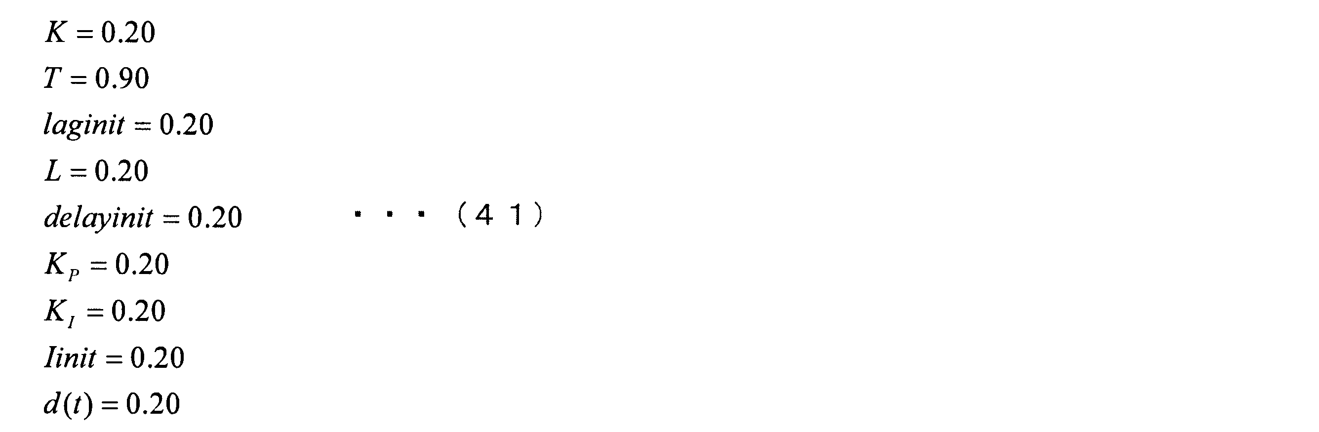
図33A~Dに、最適化後のシミュレーション結果を示す。なお、SVは、シミュレーション時に実績と同じSVを与えている。
図33A~Dに示すように、評価関数値が0.00となっていることからわかるように、PV,MVについては、実績とシミュレーションの時系列値が一致している。得られた制御モデルのパラメータは、次の式(42)の通りである。
図33A~Dに示すように、評価関数値が0.00となっていることからわかるように、PV,MVについては、実績とシミュレーションの時系列値が一致している。得られた制御モデルのパラメータは、次の式(42)の通りである。
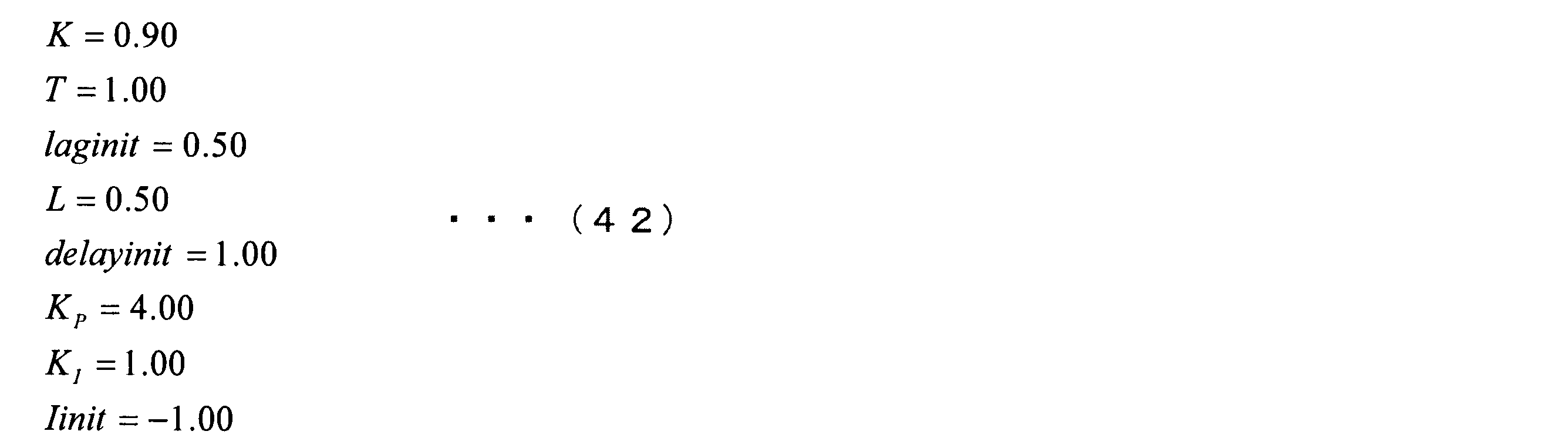
なお、外乱については、図33Dのグラフにあるように、推定された外乱は、実績の外乱と一致している。
(3例目の2)
続いて、3例目の1の例において、さらに評価関数が外乱の時系列変数値を含む場合の推定の例、すなわち3例目の2について説明する。なお、検討する理由としては、2例目の場合のように、外乱の時系列変数値を評価しないと、精確なパラメータや外乱を推定できない場合があるからである。
(3例目の2)
続いて、3例目の1の例において、さらに評価関数が外乱の時系列変数値を含む場合の推定の例、すなわち3例目の2について説明する。なお、検討する理由としては、2例目の場合のように、外乱の時系列変数値を評価しないと、精確なパラメータや外乱を推定できない場合があるからである。
図34に従って、外乱を評価する場合を説明する。
なお、制御モデルのパラメータ、外乱の真値は、式(36)と同じとする。図32A~Dが、真値のパラメータと、真値の外乱の場合の実績データを示す。なお、実績データの外乱は、ランプ状外乱やオフセットを含んでいる。
評価関数としては、次の式(43)を用いた。
なお、制御モデルのパラメータ、外乱の真値は、式(36)と同じとする。図32A~Dが、真値のパラメータと、真値の外乱の場合の実績データを示す。なお、実績データの外乱は、ランプ状外乱やオフセットを含んでいる。
評価関数としては、次の式(43)を用いた。

なお、式(43)の第3項は、外乱を0(ゼロ)に近づけるための項である。また、制約条件については、式(38)と同じである。
以上をまとめると、本具体例は、一般形を具体化した形となっている。既述の3例目の1との違いのみを、以下に説明する。
ddiは、外乱djと、同時刻で同じ値を持っている。なお、djからddiを求めるには、補間等を行うとよい。
以上をまとめると、本具体例は、一般形を具体化した形となっている。既述の3例目の1との違いのみを、以下に説明する。
ddiは、外乱djと、同時刻で同じ値を持っている。なお、djからddiを求めるには、補間等を行うとよい。
評価関数の重みは、それぞれ、式(39)と、以下の式(44)のようになる。

図3のフローチャートに基づき、最適化を行う。なお、最適化の初期値は、制約条件を満足する範囲で与えて、複数回最適化を行い、最小の評価関数の値、1.19×10⁴を持つ場合を採用した。
なお、このときの初期値は、次の式(45)の通りである。
なお、このときの初期値は、次の式(45)の通りである。

図35A~Dに、最適化後のシミュレーション結果を示す。なお、SVは、シミュレーション時に実績と同じSVを与えている。図35A~Dに示すように、PV,MVについては、実績とシミュレーションの時系列値が一致している。得られたパラメータは次の式(46)の通りである。

以上より、ゲインで33%、時定数で29%、むだ時間で6%の誤差がある。
また、外乱についても、図35Dのグラフに示すように、推定された外乱は、実績の外乱と誤差があることがわかる。
なお、外乱に対する重みWddを小さくすると、外乱の推定値の精度が良くなるが、最適化の収束に時間がかかる傾向にある。
また、外乱についても、図35Dのグラフに示すように、推定された外乱は、実績の外乱と誤差があることがわかる。
なお、外乱に対する重みWddを小さくすると、外乱の推定値の精度が良くなるが、最適化の収束に時間がかかる傾向にある。
したがって、本具体例では、外乱に単純に重みを掛けて評価した場合、若干の誤差を持つが、制御モデルのパラメータと外乱の推定は可能である。
(3例目の3)
続いて、3例目の2の例において、外乱に周波数が存在する場合に、当該周波数成分をカットするフィルタを適用し、評価関数が、フィルタ適用後の外乱の時系列変数値を含む場合の推定の例、すなわち3例目の3について説明する。
(3例目の3)
続いて、3例目の2の例において、外乱に周波数が存在する場合に、当該周波数成分をカットするフィルタを適用し、評価関数が、フィルタ適用後の外乱の時系列変数値を含む場合の推定の例、すなわち3例目の3について説明する。
本具体例は、フィルタを適用することにより、外乱をより精確に推定できる。
図36に示すように、フィルタ適用後の外乱を評価する場合を説明する。フィルタは、時定数30[s]の一次遅れ要素である。
制御モデルのパラメータ、外乱の真値は、式(36)と同じとする。図32A~Dが、真値のパラメータと、真値の外乱の場合の実績データを示す。なお、実績データの外乱は、ランプ状外乱やオフセットを含んでいる。
図36に示すように、フィルタ適用後の外乱を評価する場合を説明する。フィルタは、時定数30[s]の一次遅れ要素である。
制御モデルのパラメータ、外乱の真値は、式(36)と同じとする。図32A~Dが、真値のパラメータと、真値の外乱の場合の実績データを示す。なお、実績データの外乱は、ランプ状外乱やオフセットを含んでいる。
評価関数としては、次の式(47)を用いた。

なお、式(47)の第3項は、フィルタ後の外乱を0(ゼロ)に近づけるための項である。外乱の成分はフィルタにより低減され、評価されないため、外乱自体は大きな値を取ることができる。このため、より精確な外乱を推定可能となる。
また、制約条件については、式(38)と同じである。
以上をまとめると、本具体例は、一般形を具体化した形となっている。既述の3例目の2との違いのみを、以下に説明する。
また、制約条件については、式(38)と同じである。
以上をまとめると、本具体例は、一般形を具体化した形となっている。既述の3例目の2との違いのみを、以下に説明する。
ddiは、外乱djにフィルタを適用した後の外乱である。
評価関数の重みは、それぞれ、式(39)と、以下の式(48)のようになる。
評価関数の重みは、それぞれ、式(39)と、以下の式(48)のようになる。

図3のフローチャートに基づき、最適化を行う。なお、最適化の初期値は、制約条件を満足する範囲で与えて、複数回最適化を行い、最小の評価関数の値3.33×10²を持つ場合を採用した。
なお、このときの初期値は、次の式(49)の通りである。
なお、このときの初期値は、次の式(49)の通りである。

図37A~Dに、最適化後のシミュレーション結果を示す。なお、SVは、シミュレーション時に実績と同じSVを与えている。図37A~Dに示すように、PV,MVについては、実績とシミュレーションの時系列値が一致している。得られたパラメータは次の式(50)の通りである。

以上より、ゲインで4.4%、時定数で4.4%、むだ時間で0.7%だけの誤差しかない。
また、外乱についても、図37Dのグラフにあるように、推定された外乱は、ランプ状であっても、ほぼ一致している。
したがって、本具体例では、外乱にフィルタを適用して評価した場合、外乱を精度よく推定可能であることがわかる。
また、外乱についても、図37Dのグラフにあるように、推定された外乱は、ランプ状であっても、ほぼ一致している。
したがって、本具体例では、外乱にフィルタを適用して評価した場合、外乱を精度よく推定可能であることがわかる。
以上、今回開示された実施形態はすべての点で例示であって制限的なものではないと考えられるべきである。本発明の範囲は上記した説明ではなくて特許請求の範囲によって示され、特許請求の範囲と均等の意味及び範囲内でのすべての変更が含まれることが意図される。
本出願は、2015年3月24日出願の日本特許出願(特願2015-061059)、及び2016年1月12日出願の日本特許出願(特願2016-003776)に基づくものであり、その内容はここに参照として取り込まれる。
1 炉頂圧発電設備
2 リングスリットエレメント(RSE)
3 発電部(TRT、炉頂圧発電機)
4 高炉ガス流路
5 バイバス流路
6 バイパス弁
6a 第1バイパス弁
6b 第2バイパス弁
7 炉頂圧コントローラ
8 TRT前圧コントローラ
9 バイパス弁前圧コントローラ
10 円錐管
11 可動部
12 ケーシング
13 発電機
14 タービンの軸(ロータ)
15 動翼
16 静翼
16a 翼弁(弁機構)
17 高炉
18 サイレンサ
30 連続鋳造機
31 鋳型
32 ロール
33 タンディッシュ
34 溶鋼孔
35 浸漬ノズル
36 スライドバルブ
36a 上プレート
36b 下プレート
36c 中間プレート
37 流下孔(バルブ)
38 湯面レベル計
39 電気油圧シリンダ(アクチュエータ)
40 制御部(コントローラ)
X 溶鋼
2 リングスリットエレメント(RSE)
3 発電部(TRT、炉頂圧発電機)
4 高炉ガス流路
5 バイバス流路
6 バイパス弁
6a 第1バイパス弁
6b 第2バイパス弁
7 炉頂圧コントローラ
8 TRT前圧コントローラ
9 バイパス弁前圧コントローラ
10 円錐管
11 可動部
12 ケーシング
13 発電機
14 タービンの軸(ロータ)
15 動翼
16 静翼
16a 翼弁(弁機構)
17 高炉
18 サイレンサ
30 連続鋳造機
31 鋳型
32 ロール
33 タンディッシュ
34 溶鋼孔
35 浸漬ノズル
36 スライドバルブ
36a 上プレート
36b 下プレート
36c 中間プレート
37 流下孔(バルブ)
38 湯面レベル計
39 電気油圧シリンダ(アクチュエータ)
40 制御部(コントローラ)
X 溶鋼
Claims (9)
- 制御モデル内のパラメータと当該制御モデルが表す制御対象へ入力される外乱とを同時に推定する方法であって、前記外乱を時系列変数値として、前記制御モデルに与えることとし、前記制御対象における実績データの時系列値と、前記制御モデルをシミュレーションすることで得られたシミュレーション結果のデータの時系列値を含む評価関数が、最大又は最小となるように、前記外乱と前記パラメータとを同時に推定することを特徴とする制御モデルのパラメータと外乱との同時推定方法。
- 制御モデル内のパラメータと当該制御モデルが表す制御対象へ入力される外乱とを同時に推定する方法であって、前記外乱を時系列変数値として、前記制御モデルに与えることとし、前記制御対象における実績データの時系列値と、前記制御モデルをシミュレーションすることで得られたシミュレーション結果のデータの時系列値と、前記外乱の時系列変数値とを含む評価関数が、最大又は最小となるように、前記外乱と前記パラメータとを同時に推定することを特徴とする制御モデルのパラメータと外乱との同時推定方法。
- 前記評価関数には、実績データおよびシミュレーション結果のデータとして、制御量(PV)、操作量(MV)の少なくとも一つが与えられていることを特徴とする請求項1又は2に記載の制御モデルのパラメータと外乱との同時推定方法。
- 前記外乱に周波数成分が存在する場合には、当該周波数成分をカットするフィルタを適用した後の外乱が前記評価関数へ含まれることを特徴とする請求項1~3のいずれか一項に記載の制御モデルのパラメータと外乱との同時推定方法。
- 前記実績データの時系列値が複数群、存在する場合においては、前記パラメータを前記実績データの全ての群にて共通する値をもつパラメータと、前記実績データの各群に連動する値をもつパラメータとに分離した上で、シミュレーション結果のデータの時系列値を評価関数へ導入すると共に、前記外乱を実績データの各群に連動する時系列変数値として評価関数へ導入することを特徴とする請求項1~4のいずれか一項に記載の制御モデルのパラメータと外乱との同時推定方法。
- 前記パラメータとして、未知の初期値が採用されることを特徴とする請求項1~5のいずれか一項に記載の制御モデルのパラメータと外乱との同時推定方法。
- 前記パラメータとして、未知の定常値が採用されることを特徴とする請求項1~6のいずれか一項に記載の制御モデルのパラメータと外乱との同時推定方法。
- 前記外乱がランプ状である場合には、前記外乱の微分値を評価関数へ導入すると共に、前記外乱の微分値を積分した上で、当該積分値を前記制御モデルに与えることを特徴とする請求項2~7のいずれか一項に記載の制御モデルのパラメータと外乱との同時推定方法。
- 請求項1~8のいずれか一項に記載された制御モデルのパラメータと外乱との同時推定方法で推定されたパラメータと外乱とのうち少なくともパラメータを用いて、前記制御対象を制御することを特徴とする制御対象の制御方法。
Applications Claiming Priority (4)
| Application Number | Priority Date | Filing Date | Title |
|---|---|---|---|
| JP2015061059 | 2015-03-24 | ||
| JP2015-061059 | 2015-03-24 | ||
| JP2016003776A JP6084312B2 (ja) | 2015-03-24 | 2016-01-12 | 制御モデルのパラメータと外乱との同時推定方法、及びこの同時推定方法を用いた制御対象の制御方法。 |
| JP2016-003776 | 2016-01-12 |
Publications (1)
| Publication Number | Publication Date |
|---|---|
| WO2016152618A1 true WO2016152618A1 (ja) | 2016-09-29 |
Family
ID=56978072
Family Applications (1)
| Application Number | Title | Priority Date | Filing Date |
|---|---|---|---|
| PCT/JP2016/057948 Ceased WO2016152618A1 (ja) | 2015-03-24 | 2016-03-14 | 制御モデルのパラメータと外乱との同時推定方法、及びこの同時推定方法を用いた制御対象の制御方法 |
Country Status (1)
| Country | Link |
|---|---|
| WO (1) | WO2016152618A1 (ja) |
Cited By (2)
| Publication number | Priority date | Publication date | Assignee | Title |
|---|---|---|---|---|
| TWI677771B (zh) * | 2017-02-10 | 2019-11-21 | 日商三菱日立電力系統股份有限公司 | 模擬結果之評價裝置及方法 |
| TWI720585B (zh) * | 2019-06-14 | 2021-03-01 | 日商東芝三菱電機產業系統股份有限公司 | 資料收集裝置 |
-
2016
- 2016-03-14 WO PCT/JP2016/057948 patent/WO2016152618A1/ja not_active Ceased
Non-Patent Citations (3)
| Title |
|---|
| MANABU KANO ET AL., DEPLOYMENT OF E-FRIT IN CHEMICAL PROCESS INDUSTRY, vol. 52, no. 10, 10 October 2013 (2013-10-10), pages 898 - 903, ISSN: 0453-4662 * |
| OSAMU KANEKO ET AL.: "Identification of Linear Time-Invariant Systems under Periodic Disturbance with its Estimation", THE TRANSACTIONS OF THE INSTITUTE OF ELECTRICAL ENGINEERS OF JAPAN C, vol. 134, no. 7, 1 July 2014 (2014-07-01), pages 917 - 923, XP055317061, ISSN: 0385-4221 * |
| SHIRO MASUDA ET AL.: "An FRIT Method for Disturbance Attenuation Using Input-Output Data Generated from Disturbance Responses", THE TRANSACTIONS OF THE INSTITUTE OF ELECTRICAL ENGINEERS OF JAPAN C, vol. 131, no. 4, 1 April 2011 (2011-04-01), pages 788 - 793, ISSN: 0385-4221 * |
Cited By (2)
| Publication number | Priority date | Publication date | Assignee | Title |
|---|---|---|---|---|
| TWI677771B (zh) * | 2017-02-10 | 2019-11-21 | 日商三菱日立電力系統股份有限公司 | 模擬結果之評價裝置及方法 |
| TWI720585B (zh) * | 2019-06-14 | 2021-03-01 | 日商東芝三菱電機產業系統股份有限公司 | 資料收集裝置 |
Similar Documents
| Publication | Publication Date | Title |
|---|---|---|
| JP6084312B2 (ja) | 制御モデルのパラメータと外乱との同時推定方法、及びこの同時推定方法を用いた制御対象の制御方法。 | |
| EP2737374B1 (en) | Integrated linear/non-linear hybrid process controller | |
| CN106575104B (zh) | 使用无线过程信号的模型预测控制 | |
| CN118954657B (zh) | 基于动态过滤算法的矿井水微砂分离系统及方法 | |
| JP5817940B2 (ja) | 制御装置の設計方法および制御装置 | |
| CA2411378A1 (en) | Multi-variable matrix process control | |
| JP6111913B2 (ja) | 制御パラメータ調整システム | |
| EP2296063A2 (en) | System and method for predicting future disturbances in model predictive control applications | |
| CN120650774B (zh) | 一种热力管道的室内温度实时调控方法及其控制系统 | |
| Tseng et al. | Digital shadow identification from feed drive structures for virtual process planning | |
| CN114265368B (zh) | 航空发动机伺服控制系统组合状态自适应估计方法 | |
| JP4396541B2 (ja) | 電動機制御装置の制御パラメータ感度解析装置および電動機制御装置の制御パラメータ設定方法 | |
| Saibabu et al. | Synthesis of model predictive controller for an identified model of MIMO process | |
| Laghrouche et al. | Pressure and friction observer-based backstepping control for a VGT pneumatic actuator | |
| CN114237199A (zh) | 基于自适应比较器的航空发动机执行回路故障检测方法 | |
| WO2016152618A1 (ja) | 制御モデルのパラメータと外乱との同時推定方法、及びこの同時推定方法を用いた制御対象の制御方法 | |
| Liu et al. | Velocity estimation of robot manipulators: An experimental comparison | |
| JP2006227793A5 (ja) | ||
| CN120701640B (zh) | 一种适用复杂情况的液压升降系统同步控制系统及方法 | |
| JP2005275588A (ja) | 電動機制御装置制御パラメータ感度解析装置 | |
| Wu et al. | A comprehensive decoupling control strategy for a gas flow facility based on active disturbance rejection generalized predictive control | |
| KR20190001477A (ko) | 최적 듀얼 제어를 위한 방법과 체계 | |
| JP6372217B2 (ja) | 連続鋳造鋳型内の湯面変動の状態推定方法、及び、装置 | |
| CN119268692A (zh) | 一种半球谐振陀螺仪姿态漂移误差补偿方法 | |
| CN106371419A (zh) | 用于监视控制回路的运行的诊断装置和诊断方法 |
Legal Events
| Date | Code | Title | Description |
|---|---|---|---|
| 121 | Ep: the epo has been informed by wipo that ep was designated in this application |
Ref document number: 16768521 Country of ref document: EP Kind code of ref document: A1 |
|
| NENP | Non-entry into the national phase |
Ref country code: DE |
|
| 122 | Ep: pct application non-entry in european phase |
Ref document number: 16768521 Country of ref document: EP Kind code of ref document: A1 |