WO2011148639A1 - 分子間力のシミュレーション手法 - Google Patents
分子間力のシミュレーション手法 Download PDFInfo
- Publication number
- WO2011148639A1 WO2011148639A1 PCT/JP2011/002927 JP2011002927W WO2011148639A1 WO 2011148639 A1 WO2011148639 A1 WO 2011148639A1 JP 2011002927 W JP2011002927 W JP 2011002927W WO 2011148639 A1 WO2011148639 A1 WO 2011148639A1
- Authority
- WO
- WIPO (PCT)
- Prior art keywords
- potential
- calculation
- interaction
- model
- molecules
- Prior art date
- Legal status (The legal status is an assumption and is not a legal conclusion. Google has not performed a legal analysis and makes no representation as to the accuracy of the status listed.)
- Ceased
Links
Images





Classifications
-
- G—PHYSICS
- G16—INFORMATION AND COMMUNICATION TECHNOLOGY [ICT] SPECIALLY ADAPTED FOR SPECIFIC APPLICATION FIELDS
- G16C—COMPUTATIONAL CHEMISTRY; CHEMOINFORMATICS; COMPUTATIONAL MATERIALS SCIENCE
- G16C10/00—Computational theoretical chemistry, i.e. ICT specially adapted for theoretical aspects of quantum chemistry, molecular mechanics, molecular dynamics or the like
Definitions
- the present invention relates to a calculation method for obtaining an interaction between molecules by performing a molecular simulation (simulation based on a molecular dynamics method) using a computer, and in particular, a potential obtained by combining an electrostatic interaction potential and a non-bonding action potential. It is a calculation method that can be created and applied to molecular motion simulations of polymers and is suitable for evaluation of new materials, etc., and it has high calculation accuracy and convergence of calculation even for model systems in which charges such as hydrogen bonds mainly work
- the present invention relates to a high-speed intermolecular interaction calculation method.
- Patent Document 1 discloses a method of building a filler molecule model and measuring the interaction from the distance between the models. However, since it is a molecular model, there is a problem that the interaction regarding each individual atom is “rounded” and cannot be measured in detail.
- Patent Document 2 discloses a method for calculating the adsorption energy between carbon molecules and surrounding molecules based on carbon molecules. However, the surrounding molecules are also modeled, and there is a problem that it is impossible to measure in detail the interaction between atoms that are truly involved in adsorption and other surrounding atoms.
- the calculation objects of Patent Documents 1 and 2 are limited between fillers or between low-molecular model compounds obtained by virtually decomposing a carbon model and a polymer.
- a detailed charge structure or coarse structure at the atomic level in a united atom modem is used. Since the calculation that reflects the charge structure over the entire polymer in the visualization model and the molecular motion state of the molecules existing in the system cannot be performed, the influence of the electrostatic interaction potential of the model system in which charges such as hydrogen bonds mainly act is affected. It is a model calculation system with high calculation accuracy and high convergence speed.
- an object of the present invention is to solve the above-mentioned problems of the prior art, and has high calculation accuracy even when applied to a model system in which charges such as hydrogen bonds mainly act using a computer, and the convergence speed of calculation is high. It is to provide a method for calculating a fast non-bonded interaction potential. Still another object is to provide a molecular interaction calculation method that can be applied to a molecular motion simulation of a polymer by using the non-bonded interaction potential and is suitable for evaluation of a new material.
- the present inventor diligently studied the numerical calculation of a calculation model system under the action of Coulomb force, found a calculation method of non-bonded interaction potential, and completed the present invention.
- the calculation method of the non-bonded interaction potential of the present invention is a calculation method for calculating the non-bonded interaction potential by performing a simulation by a molecular dynamics method using a computer. Selecting molecules and using them as model molecules; Obtaining the charge of the model molecule, applying the obtained charge to each molecule, calculating the non-bonded interaction potential (A) by moving the model molecule in a three-dimensional manner in the system, A step of calculating a non-bonded interaction potential (B) under the action of a non-Coulomb force by moving the model molecule three-dimensionally in the system with zero electrostatic interaction, and the calculated non-bonded interaction And calculating a Lennard-Jones potential (C) by comparing the potential (A) with the non-bonded interaction potential (B) under the non-Coulomb force action.
- the intermolecular interaction calculation method of the present invention includes a step of applying to a molecule existing in the system based on the correction term (C) of the Lennard-Jones potential.
- the model molecule preferably includes any one of calculation units made of a polymer.
- a calculation method for a non-bonded interaction potential that has high calculation accuracy and high calculation convergence speed even when applied to a model system in which charges such as hydrogen bonds mainly act using a computer. It becomes possible to do.
- an intermolecular interaction calculation method that can be applied to a molecular motion simulation of a polymer by applying the non-bonded interaction potential and is suitable for evaluation of a new material. It becomes possible to do.
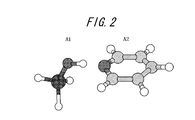
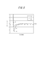
- FIG. 3 is a schematic diagram showing non-bonding interaction potentials (P1, P3) and electrostatic interaction potentials (P2, P4) between atoms constituting the model molecule A1-A2. It is a schematic diagram showing the structure of model molecules A1-A2. It is a schematic diagram which shows the non-bonding interaction potential (P5: A, P6: B) and electrostatic interaction potential (P7) between model molecules. It is a schematic diagram showing the structure of model molecules C1-C2. It is a comparison figure which shows the non-bonding interaction potential (P5: A, P8: C) between model molecules. It is explanatory drawing which shows the non-bonding potential (LJ type) between general particles.
- FIG. 7 is a diagram showing a configuration of a non-bonded interaction potential and intermolecular interaction calculation system as one embodiment of the calculation method of the present invention
- FIG. 8 shows a non-bonded interaction potential and molecules shown in FIG. It is explanatory drawing of the electric system principal part structure of the computer which comprises an interaction calculation system.
- the computer 2 includes a computer main body 3 that performs calculation of non-bonding interaction potential and intermolecular interaction calculation in accordance with a pre-stored processing program, and an input device 4 such as a keyboard for inputting various conditions for analysis. And a display 5 for displaying calculation results of the computer main body 3 and the like. Further, the computer main body 3 includes a recording medium driving unit 6 (hereinafter referred to as the driving unit 6) into which the recording medium 7 can be inserted and removed.
- the driving unit 6 recording medium driving unit 6
- the computer 2 includes a CPU (Central Processing Unit) 3a that controls the operation of the entire apparatus, a ROM 3b that stores various programs including a control program for controlling the computer 2, various parameters, and the like, A RAM 3c that temporarily stores various data, an HDD (hard disk drive) 3d that stores various data and processing programs, an operation input detection unit 3e that detects an operation on the input device 4, and various information on the display 5 A display driver 3f for controlling the display of the recording medium and a recording medium I / F unit 3g for inputting / outputting data to / from the recording medium 7 mounted on the drive unit 6.
- a CPU Central Processing Unit
- ROM 3b that stores various programs including a control program for controlling the computer 2, various parameters, and the like
- a RAM 3c that temporarily stores various data
- an HDD (hard disk drive) 3d that stores various data and processing programs
- an operation input detection unit 3e that detects an operation on the input device 4
- a display driver 3f for controlling the display of the recording medium and a recording medium I
- the CPU 3a, ROM 3b, RAM 3c, HDD 3d, operation input detection unit 3e, display driver 3f, and recording medium I / F unit 3g are connected to each other via a system bus BUS 3h. Therefore, the CPU 3a accesses the ROM 3b, RAM 3c, HDD 3d, displays various information on the display 5 via the display driver 3f, and the recording medium 7 attached to the drive unit 6 via the recording medium I / F unit 3g. Each can be accessed. Further, the CPU 3a can always grasp the key operation on the input device 4.
- processing programs, data, and the like can be read from and written to the recording medium 7 using the drive unit 6. Therefore, various processing programs and data may be recorded in the recording medium 7 in advance, and each processing program recorded in the recording medium 7 may be executed via the drive unit 6. Further, each processing program recorded in the recording medium 7 may be stored (installed) in the HDD 3d and executed. Furthermore, data or a program may be exchanged and executed with an external server device (not shown) connected to the simulation device 1. Examples of the input device 4 include a keyboard, a mouse, and a touch panel.
- Examples of the recording medium 7 include a recording tape, a floppy (registered trademark) disk, an optical disk such as a CD-ROM and a DVD, and a magneto-optical disk such as an MD and an MO. Further, a corresponding read / write device may be used.
- the configuration of the non-bonded interaction potential and intermolecular interaction calculation system 1 shown in FIG. 7 is an example, and a known configuration can be appropriately changed as necessary.
- molecular dynamics (MD) calculation is a kind of simulation using a computer device, and is an aggregate of many atoms or molecules based on the molecular structure of the polymer material to be analyzed.
- a model in which particles are arranged is set, and Newton's equation of motion is applied as if all the arranged particles obey classical mechanics, and the movement of all particles at each time is tracked.
- the microscopic motion of the particles can be tracked as accurately as possible, and the properties and motions of the substance can be clarified without depending on the experimental results. Further, by adjusting the tracking time and the like, an accurate simulation result that does not depend on the initial arrangement of particles can be obtained.
- a force based on a Lennard-Jones (LJ) potential is generally used as a force acting between particles.
- the LJ potential U (r) is expressed by Equation 1.
- U (r) 4 ⁇ [( ⁇ 0 / r) 12 ⁇ ( ⁇ 0 / r) 6 ] Equation 1
- r is the distance between particles.
- ⁇ 0 is a reference length.
- ⁇ is a coefficient reflecting interparticle forces.
- the -6th power gravitational force term is due to the dispersion force between two atoms, that is, the interaction between dipoles and dipoles, while the -12th power repulsion term is the repulsive force due to the overlap of electron clouds, that is, Pauli exclusion. It is by the law.
- U (r) when r is ⁇ 0 or less, U (r) is a very large value of 0 or more, and when r> ⁇ 0 , U (r) is 0 or less. Value.
- U (r) takes the minimum value ⁇ . Since the force acting between the particles is expressed by potential differentiation, a large repulsive force is generated between the particles under the condition of r ⁇ 2 1/6 ⁇ 0 under the LJ potential U (r), and r> 2 1 / In the state of 6 ⁇ 0 , attractive force is generated between particles.
- the parameter ⁇ 0 of the LJ potential U (r) corresponds to the sum of the radii of adjacent particles, and can be interpreted as corresponding to the particle diameter between the same type of particles.
- a method of changing the upper limit distance (cutoff distance) for calculating these potentials is generally performed.
- the upper limit distance (cut-off distance) is generally set to 2.5 ⁇ 0. It is what.
- a force based on Coulomb's law is generally used as an electrostatic interaction potential as a force acting between charged particles.
- Coulomb force F c (r) is expressed by Equation 2.
- F c (r) (1 / 4 ⁇ 0 ) [Q 1 ⁇ Q 2 / r 2 ] Equation 2
- r is the distance between particles.
- ⁇ 0 is the dielectric constant of vacuum
- Q 1 and Q 2 are the electric charges of each particle.
- Q 1 and Q 2 are negative values between different kinds of charges and represent attractive forces, and the same kinds of charges are positive values and represent repulsive forces.
- the size of a calculation unit of a large-scale calculation system includes a calculation method for each atom and a calculation method using coarse graining.
- Coarse graining is one of the methods for calculating a system composed of a large number of atoms, and is a calculation method using an aggregate of a plurality of atoms or molecules as a calculation unit. Coarse graining greatly reduces the number of calculation units, and a system consisting of a large number of atoms can be handled by a general general-purpose computer. However, if the coarse-graining is too rough, the characteristics of the molecular structure are lost and problems such as slipping through occur, and therefore an appropriate coarse-graining level needs to be selected.
- the united atom model that handles carbon atoms and hydrogen atoms as one aggregate is useful for examining the effects of hydrogen bonds in detail.
- the united atom model it is possible to examine in detail the electrostatic interaction due to charges in hydrogen bonds and the like that cannot be obtained in Patent Documents 1 and 2, down to the atomic level.
- Create a monomer unit (the simplest unit in which multiple atoms coexist) in a system for confirming the interaction between molecules, set the charge and LJ potential for each coarse-grained particle, and perform calculations Is preferred.
- a polymer material such as a rubber material is a polymer in which rubber molecules such as isoprene composed of a plurality of atoms are polymerized in a chain, and the molecules constituting the polymer are intertwined with each other. And make a system. It is not realistic to handle a huge amount of atoms with a computer one by one. In view of this, coarse-graining in a fine-grained calculation unit that is a calculation unit of roughness that can be handled by a computer and that can grasp the characteristics of the polymer system that is the purpose of calculation is used for the calculation.
- Coarse-grained molecular dynamics that represents a system to be simulated as a system in which a large number of coarse-grained units that aggregate multiple atoms or molecules are gathered, and that performs simulation by calculating the interaction between the coarse-grained units. It can be used to simulate large-scale systems over a long period of time. For example, in the case of a rubber molecule in which isoprene is polymerized, polyisoprene in which a predetermined number of isoprene is polymerized in a chain form is used as a coarse-grained unit, and this coarse-grained unit is combined in a plurality of chains to represent a rubber molecule. Rubber molecules can be assembled to represent a rubber material.
- the number of particles is approximately 1/10 to 1/100, and the calculation time for the interaction between particles is proportional to the square of the number of particles. 1/10 2 to 1/10 4, weight also shorter time 1/10 2 to 1/10 3, the time step that is inversely proportional to the square root of the mass can be 10-30 times and faster, even combining size 5 -10 times, spatial scale can be expanded to 5-10 times.
- modified polymers are used, and these need to be modeled.
- the modified polymer refers to a material component having a property that a part of the polymer, preferably a terminal portion thereof, is chemically bonded to the filler or has a high affinity.
- a modified polymer having an amine functional group chemically bonded to carbon black or having a high affinity at the terminal a modified polymer having an alkoxy functional group or silanol functional group chemically bonded to silica or having a high affinity at the terminal, or an amine functional group
- a modified polymer having an alkoxy functional group and a silanol functional group at the same time a modified polymer having an alkoxy functional group and a silanol functional group at the same time.
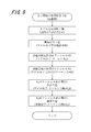
- FIG. 9 is a flowchart showing an intermolecular interaction calculation processing procedure performed by the non-bonded interaction potential and intermolecular interaction calculation system 1 in one embodiment
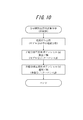
- FIG. 10 is performed by a conventional intermolecular interaction calculation system. It is a flowchart which shows the procedure in one embodiment of a calculation process.
- the CPU 3a executes the following processing according to each processing program loaded into the RAM 3c as necessary.
- Step 1 Selection of model molecule
- Two molecules are selected from a plurality of molecules existing in the system, and these are used as model molecules.
- a monomer unit (the simplest unit in which a plurality of atoms coexist) is created as a calculation unit. This is because the reference potential (A) reflecting the effect of electric charges is calculated at high speed while reducing the calculation load.
- Monomer unit data is transmitted from the input device 4 or the recording medium 7 or the like to the computer 2, and upon receiving a start signal, arithmetic processing or the like is performed by the CPU 3a or the like.
- the model molecule preferably includes at least one calculation unit made of a polymer. This is because such a polymer model molecule has a plurality of similar sequences, so that modeling is easy and calculation is easy at high speed. Therefore, it is useful for polymer evaluation, particularly for new material evaluation. However, it can also be applied to interactions with small molecules.
- the model molecule is described as one model molecule, there is no charge bias and the charge amount is zero.
- the model molecule is described locally, there is a charge bias, and the charge bias has anisotropy. More preferably, it contains a model molecule. When the model intermolecular distance is less than ⁇ 0 , the repulsive force due to the overlap of electron clouds is dominant and the electrostatic interaction can be ignored.
- the distance between model molecules is about the diameter of a model molecule of about ⁇ 0 to 2 ⁇ 0, the difference in Coulomb force due to the difference between the positive charge and the negative charge polarized in the model molecule is significant, and the electrostatic interaction becomes significant.
- the distance between the model molecules exceeds the cutoff distance of about 2.5 ⁇ 0, the difference in the Coulomb force due to the difference between the positive charge and the negative charge polarized in the model molecule becomes small, and the whole model molecule is zero as a whole. It can be regarded as an electric charge. It can be seen that the shape of the potential function approaches the LJ potential.
- the inventors have found that the electrostatic interaction potential can be approximated by providing a correction term with the LJ potential.
- the electrostatic interaction potential (FIGS. 1P2 and P4) between the single charged atoms that make up the model molecule (FIG. 2) cannot be approximated at all by the LJ potential.
- FIG. 3P5 it has been found that by calculating between model molecules that are polarized and have both positive and negative charges, it can be approximated to a function form close to the LJ potential (FIG. 3P5).
- a high-precision approximation with the LJ potential correction term (C, FIG. 5P8) by adjusting the interaction parameters only for a few particles in the model molecule where electrostatic interactions tend to appear significantly (FIG. 4).
- the interaction parameters can be set only for a few particles in the model molecule where electrostatic interactions tend to appear remarkably. Adjustment is a technology that cannot be easily conceived. Furthermore, surprisingly, not only the qualitative aspect of calculation accuracy but also the cut-off distance can be set by adjusting the interaction parameter, and a remarkable effect can be obtained in terms of the quantitative aspect of calculation speed. This is unexpected and not easily conceived by those skilled in the art.
- the model molecule having anisotropy in the electric charge can be reversed by generating a rotational moment by electrostatic interaction. This is because a model molecule in which the same kind of charges are close to each other can be easily rotated to a stable energy state at high speed, so that a calculation result with high accuracy in conformity with an actual system can be obtained at high speed.
- Step 2 Charge application to model molecule
- the charge of the model molecule is obtained, and the obtained charge is applied to each molecule.
- a charge numerical calculation method such as a molecular orbital method.
- the molecular orbital method is a method using quantum mechanics, which clarifies the structure and physical properties of a target molecule by solving Schrodinger's wave equation.
- the monomer unit data transmitted to the computer 2 is subjected to arithmetic processing by the CPU 3a or the like by molecular orbital method software (CNDO, INDO, MINDO, PM3, Gaussian, etc.), and each monomer unit particle (atom, Charges are set in atomic groups and coarse-grained units.
- the calculation is completed by recording numerical data relating to the charge, which is the calculation result performed by the CPU 3a, etc., from the RAM 3c to the recording medium 7, etc.
- the charge to be applied is described as one model molecule as a whole, the charge is not biased and the amount of charge is zero.
- the model molecule is described locally, there is a charge bias, and the charge bias is anisotropic. It is preferable to include a model molecule having a property. This is because the calculation with the LJ potential correction term (C) with high calculation accuracy is possible, and the calculation speed can be increased by setting the cutoff distance or the like.
- the model molecule having anisotropy in the electric charge can be reversed by generating a rotational moment by electrostatic interaction. This is because it can easily transition to a stable energy state at high speed, so that a high-precision calculation result that matches the actual system can be obtained at high speed.
- Step 3 Calculation of non-bonded interaction potential (A) between model molecules
- the non-bonding interaction potential (A) is calculated by moving the model molecule three-dimensionally in the system. Specifically, the data relating to the position and movement of the monomer unit transmitted to the computer 2 and the data relating to the charge obtained in step 2 are processed by the CPU 3a or the like using the LJ potential and electrostatic interaction calculation software, and the model is obtained.
- the non-bond interaction potential (A) between the molecules is calculated, and the calculation result performed by the CPU 3a or the like is recorded from the RAM 3c to the recording medium 7 or the like, thereby completing the calculation.
- Step 4 Calculation of non-bonded interaction potential (B) between model molecules
- the electrostatic interaction is set to 0, and the model molecule is moved three-dimensionally in the system to calculate the non-bonding interaction potential (B) under the non-Coulomb force action.
- “setting the electrostatic interaction to 0” means using the data of charge 0 without using the charge application data in step 2.
- the data relating to the position and movement of the monomer unit whose charge data is 0 transmitted to the computer 2 is processed by the CPU 3a or the like using the LJ potential calculation software, and the non-bonding interaction potential between the model molecules.
- (B) is calculated, and the calculation result performed by the CPU 3a or the like is recorded on the recording medium 7 or the like from the RAM 3c, thereby completing the calculation.
- Step 5 Calculation of non-bonded interaction potential correction term (C) between model molecules
- the LJ potential correction term (C) is calculated by comparing the non-bond interaction potential (A) with the non-bond interaction potential (B) under the non-Coulomb force action.
- calculating the LJ potential correction term (C) means calculating the LJ potential (C) corrected at the same time.
- “compare” means performing comparison calculation by parameter fitting calculation or the like. For example, in a simple model system, it is possible to cope by comparing by arithmetic calculation such as simple subtraction.
- the CPU 3a is calculated by calculation software based on data on the non-bonded interaction potential (A) transmitted from the recording medium 7 or the like to the computer 2 and the non-bonded interaction potential (B) under the non-Coulomb force action.
- the corrected non-bonding interaction LJ potential (C) between the model molecules is calculated simultaneously with the correction term, and the calculation result performed by the CPU 3a etc. is recorded from the RAM 3c to the recording medium 7 etc. To finish the calculation.
- Step 6 Application of non-bonded interaction LJ potential correction term (C) to molecules in system
- the Coulomb force-corrected LJ-type non-bonded interaction LJ potential correction term (C) obtained in step 5 is applied to molecules existing in the system.
- the numerical data regarding is recorded from the RAM 3c to the recording medium 7 or the like, thereby completing the calculation.
- the amount of change in the energy of the entire system becomes, for example, 1/1000 (installed value) in the unit time (set time)
- new material evaluation can be performed using the generated calculation result.
- Example 1 As a computer, a workstation using an Intel CPU Xeron 3.0 GHz was used. As numerical calculation software, cogac 6.1 by OCTA project was used. As a system for confirming electrostatic interaction, one unit of each of the SiO monomer and the pyridine monomer was selected as the model molecule A1-A2 (step 1: see FIG. 2). Charges were set for each particle (SiO monomer: Si, O, H atom, pyridine monomer: CH atomic group, N atom) as calculated by molecular orbital method software (Gaussian) (step 2).
- SiO monomer Si, O, H atom
- pyridine monomer CH atomic group, N atom
- the position of the SiO monomer was fixed, the pyridine monomer was moved, and the non-bonding interaction potential (A) under the action of Coulomb force acting between them was calculated (step 3: see FIG. 3P5).
- the reference length ⁇ 0 of the LJ potential is shown in the upper part of Table 1
- the charge having the anisotropy shown in Table 2 was used for the charge used for calculating the Coulomb potential.
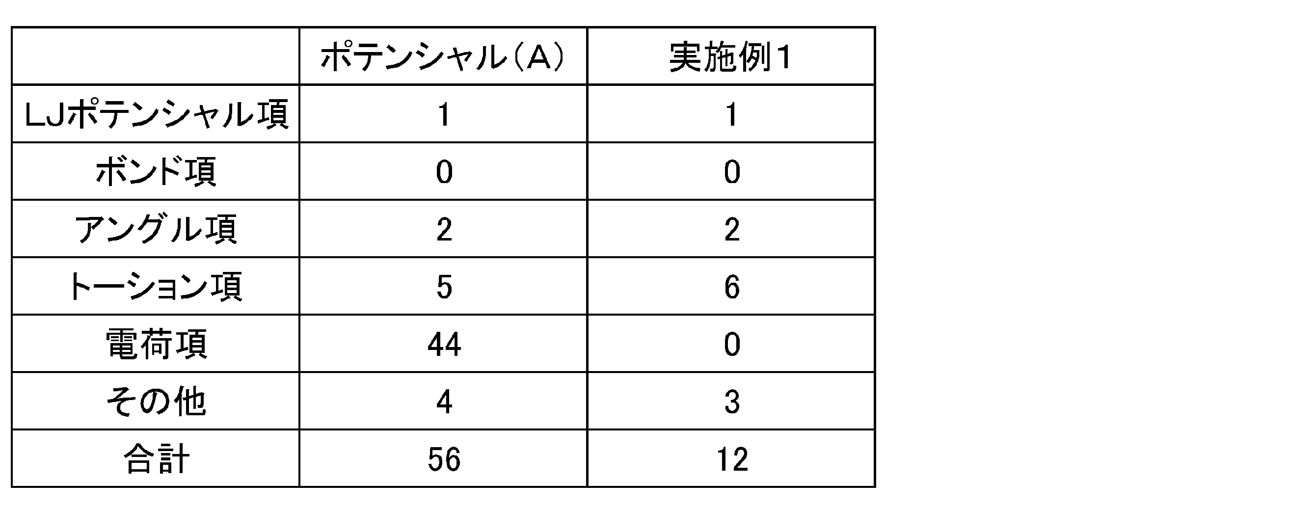
- Table 4 shows the calculation time required for calculating the potential (A).
- Table 4 shows the calculation time required for 140,000 steps between monomers in terms of seconds.
- the charge is set to 0 (eliminates electrostatic interaction), the position of the SiO monomer is fixed again, the pyridine monomer is moved, and the non-bonding interaction potential under the non-Coulomb force action acting between them (B) was calculated (step 4: see FIG. 3P6).
- calculation model C1-C2 parameters of a plurality of particles (here, SiO monomer: 1 atom each of Si, O, and H, pyridine monomer: CH atom group ⁇ 2, 6 particles of N atom: see FIG. 4) are corrected.
- an LJ potential correction term (C) in which the Coulomb force was corrected was calculated (Step 5: see FIG. 5P8).
- the LJ potential correction term (C) and potential (A) obtained by sequentially setting the parameters of a plurality of particles were compared and calculated.
- Table 3 shows the corrected LJ potential (C) parameters.
- the calculation time required for the calculation is shown in Table 4, and the calculation result is shown in FIG.
- Table 1 shows the parameters of the LJ potential (A).
- the reference length ⁇ 0 of the LJ potential (A) between the atoms is shown in the upper part of Table 1, and the parameter ⁇ of the LJ potential (A) is shown in the lower part of Table 1.
- Table 2 shows the charge setting values. Here, the numbers assigned to the respective atoms are shown in FIG.
- Table 3 shows the corrected LJ potential (C) parameters.
- the reference length ⁇ 0 of the LJ potential (C) between each atom is common to the LJ potential (A) shown in the upper part of Table 1.
- the parameter ⁇ of the LJ potential (C) is shown in Table 3 from the values shown in the lower part of Table 1 only between the atoms marked with circles in FIG. The value was changed to the calculated value.
- the numbers assigned to the respective atoms are shown in FIG.
- Table 4 shows the calculation time required to calculate the corrected LJ potential (C) shown in Example 1 and the calculation time required to calculate the potential (A), which is a conventional technique.
- the calculation time required to calculate 140,000 steps for each monomer is shown in seconds for each term.
- the calculation element shown in Example 1 is a model molecule with one molecule
- the calculation speed can be quantitatively compared.
- a set time is set.
- the potential (A) which is the prior art, did not converge, and the calculation speed could not be compared quantitatively.
- the corrected LJ potential (C) as an example, the calculation sufficiently converged in a calculation time required for normal LJ potential calculation, for example, 8 hours. Since the number of constituent elements of the molecule is 4000 times (in the case of 20 polymers) compared to the model molecule of one molecule, it is estimated that the calculation speed has been increased by about 30 times.
- the threshold cut-off distance
- the threshold can be set especially in the calculation of the charge term in a system with a large number of calculation elements. This is because the difference in the calculation amount exponentially increases with or without the threshold as the calculation scale increases, so the difference in calculation speed increases exponentially. This is considered to have led to a qualitative difference in the result of being incomputable.
Landscapes
- Engineering & Computer Science (AREA)
- Computing Systems (AREA)
- Theoretical Computer Science (AREA)
- Physics & Mathematics (AREA)
- Health & Medical Sciences (AREA)
- General Health & Medical Sciences (AREA)
- Spectroscopy & Molecular Physics (AREA)
- Life Sciences & Earth Sciences (AREA)
- Bioinformatics & Cheminformatics (AREA)
- Bioinformatics & Computational Biology (AREA)
- Management, Administration, Business Operations System, And Electronic Commerce (AREA)
Abstract
静電相互作用ポテンシャルと非結合作用ポテンシャルを組み合わせたポテンシャルを作成し、水素結合のような電荷が主として作用するモデル系に関しても計算精度が高く、かつ、計算の収束速度が速い分子間相互作用計算手法を提供することを目的とする。 解決手段としては、系内に存在する複数の分子のうちから2分子をモデル分子とする工程と、前記モデル分子の電荷を求めて分子に付与する工程と、非結合相互作用ポテンシャル(A)を算出する工程と、非結合相互作用ポテンシャル(B)を算出する工程と、前記非結合相互作用ポテンシャル(A)と前記非クーロン力作用下での非結合相互作用ポテンシャル(B)を比較してLennard-Jonesポテンシャル補正項(C)を算出する工程と、を有することを特徴とする。
Description
本発明は、計算機を用いて分子シミュレーション(分子動力学法によるシミュレーション)を行うことで分子間の相互作用を求める計算手法に関し、特に、静電相互作用ポテンシャルと非結合作用ポテンシャルを組み合わせたポテンシャルを作成し高分子の分子運動シミュレーションなどに適応可能で、新規材料の評価などに好適な計算手法であって、水素結合のような電荷が主として作用するモデル系に関しても計算精度が高くかつ計算の収束速度が速い分子間相互作用計算手法に関するものである。
従来からゴムや樹脂等の高分子ポリマーにカーボンブラックやシリカ等のフィラーを配合すると補強効果があることが知られており、高分子ポリマーにフィラーを配合したゴム材料等の高分子材料が、例えば、自動車用タイヤ等の高分子材料製品に適用されている。前記高分子材料は、高分子を含む材料であれば特に限定されないが、好ましくは天然ゴム、合成ゴム、合成樹脂等を含む有機高分子材料が好適である。このようなフィラー充填ゴム等の高分子材料では、分子動力学法(特許文献1参照)や第一計算原理(特許文献2参照)に基づくシミュレーション方法等が行われている。
特許文献1にはフィラー分子のモデルを構築し、モデル間距離から相互作用を測定する方法が開示されている。但し、分子モデルであることから、内在する個々の原子に関する相互作用は「まるめ」られており、詳細には測定できないという問題がある。
また、特許文献2にはカーボン分子を基準として、それらと周囲の分子との吸着エネルギーを算出する方法が開示されている。但し、周囲分子もモデル化されており、周囲分子のうち真に吸着に関与する原子とその他の周囲原子との相互作用については詳細に測定できないという問題がある。
また、これら特許文献1~2の計算対象は、フィラー同士間やカーボンモデルと高分子を仮想分解した低分子モデル化合物間に限られ、例えばユナイテッドアトムモデムでの原子レベルの詳細な電荷構造や粗視化モデルでの高分子全体にわたる電荷構造や系に存在する分子の分子運動状態を反映した計算ができないため、水素結合のような電荷が主として作用するモデル系の静電相互作用ポテンシャルの影響を計算精度が高くかつ計算の収束速度が速く考慮できないモデル計算系である。
また、特許文献2にはカーボン分子を基準として、それらと周囲の分子との吸着エネルギーを算出する方法が開示されている。但し、周囲分子もモデル化されており、周囲分子のうち真に吸着に関与する原子とその他の周囲原子との相互作用については詳細に測定できないという問題がある。
また、これら特許文献1~2の計算対象は、フィラー同士間やカーボンモデルと高分子を仮想分解した低分子モデル化合物間に限られ、例えばユナイテッドアトムモデムでの原子レベルの詳細な電荷構造や粗視化モデルでの高分子全体にわたる電荷構造や系に存在する分子の分子運動状態を反映した計算ができないため、水素結合のような電荷が主として作用するモデル系の静電相互作用ポテンシャルの影響を計算精度が高くかつ計算の収束速度が速く考慮できないモデル計算系である。
一方、近年の材料技術、解析技術、計算技術の進歩により、極性基含有高分子などの新しい材料と充填剤表面の相互作用や充填剤表面自体の詳細についても、従来は計算が困難であり寄与も小さいとみなされていたが、水素結合のような電荷が主として作用するモデルについて、数原子程度の小規模計算モデル系ながら数値計算が試みられ、電荷の寄与も無視しえない大きさがあることが分かってきた(図1aのP2、図1bのP4参照)。ここで、静電相互作用ポテンシャルとしてはクーロンの法則が、非結合作用ポテンシャルとしてはLenard-Jones(LJ)ポテンシャルが広く用いられている。
しかし、クーロンの法則とLJポテンシャルを単純に組み合わせ又は両方を作用させたポテンシャルによる計算方法では、電荷を考慮して分子動力学を用いる場合、もともと大きい計算量がさらに数十倍以上となって計算負荷が膨大となる。このため、水素結合のような電荷が主として作用するモデルでは、高分子などの大規模計算が困難であるという問題がある。
しかし、クーロンの法則とLJポテンシャルを単純に組み合わせ又は両方を作用させたポテンシャルによる計算方法では、電荷を考慮して分子動力学を用いる場合、もともと大きい計算量がさらに数十倍以上となって計算負荷が膨大となる。このため、水素結合のような電荷が主として作用するモデルでは、高分子などの大規模計算が困難であるという問題がある。
クーロンの法則をLJポテンシャルで近似することも考えられるが、両者の性質が大きく相違するため、単純に近似できる形ではないという問題がある。なぜなら、静電相互作用は粒子間の電荷の組み合わせにより、正と負の値をもつ(図1のbP4、図1aのP2参照)が、LJポテンシャル(図1aのP1、図1bのP3参照)では正と負の両方を1つの式で表現することはできないからである。さらに、静電相互作用は距離rの2乗に反比例するのに対し、LJポテンシャルはrの12乗に反比例する斥力とrの6乗に反比例する引力で表わされるため、そもそも容易に近似できる形ではない(図1参照)という問題がある。
さらに、計算の高速化に関しては、LJポテンシャルでは、影響を無視できる範囲をしきい値(カットオフ距離)として計算範囲を狭め計算の高速化が実施できるのに対し、クーロンの法則では、遠距離まで影響があるためしきい値を小さく設定できず計算の高速化が困難であるという問題がある(図1aP2、図1bのP4参照)。高速化のためには、並列計算化などの対応方法もあるが、計算コストが飛躍的に増大するという問題がある。
このように、大規模計算に対する要望は大きいものの、確立した計算手法はいまだ得られていないのが現状である。
さらに、計算の高速化に関しては、LJポテンシャルでは、影響を無視できる範囲をしきい値(カットオフ距離)として計算範囲を狭め計算の高速化が実施できるのに対し、クーロンの法則では、遠距離まで影響があるためしきい値を小さく設定できず計算の高速化が困難であるという問題がある(図1aP2、図1bのP4参照)。高速化のためには、並列計算化などの対応方法もあるが、計算コストが飛躍的に増大するという問題がある。
このように、大規模計算に対する要望は大きいものの、確立した計算手法はいまだ得られていないのが現状である。
そこで、本発明の目的は、上記従来技術の問題を解決し、計算機を用いて水素結合のような電荷が主として作用するモデル系に適用しても計算精度が高く、かつ、計算の収束速度が速い非結合相互作用ポテンシャルの計算手法を提供することにある。さらに他の目的は、該非結合相互作用ポテンシャルを用いることで高分子の分子運動シミュレーションなどに適応可能で、新規材料の評価などに好適な分子間相互作用計算手法を提供することにある。
本発明者は、上記課題を解決すべく、クーロン力作用下の計算モデル系の数値計算を鋭意検討し、非結合相互作用ポテンシャルの計算手法を見出し、本発明を完成させるに至った。
本発明の非結合相互作用ポテンシャルの計算手法は、計算機を用いて分子動力学法によるシミュレーションを行うことで非結合相互作用ポテンシャルを求める計算手法において、系内に存在する複数の分子のうちから2分子を選択しそれらをモデル分子とする工程と、
前記モデル分子の電荷を求めて、求まった電荷をそれぞれの分子に付与する工程と、前記モデル分子を系内で3次元的に動かすことで非結合相互作用ポテンシャル(A)を算出する工程と、静電相互作用を0として、前記モデル分子を系内で3次元的に動かすことで非クーロン力作用下の非結合相互作用ポテンシャル(B)を算出する工程と、算出された前記非結合相互作用ポテンシャル(A)と前記非クーロン力作用下での非結合相互作用ポテンシャル(B)とを比較演算することで、Lennard-Jonesポテンシャル(C)を算出する工程と、を有することを特徴とする。
前記モデル分子の電荷を求めて、求まった電荷をそれぞれの分子に付与する工程と、前記モデル分子を系内で3次元的に動かすことで非結合相互作用ポテンシャル(A)を算出する工程と、静電相互作用を0として、前記モデル分子を系内で3次元的に動かすことで非クーロン力作用下の非結合相互作用ポテンシャル(B)を算出する工程と、算出された前記非結合相互作用ポテンシャル(A)と前記非クーロン力作用下での非結合相互作用ポテンシャル(B)とを比較演算することで、Lennard-Jonesポテンシャル(C)を算出する工程と、を有することを特徴とする。
本発明の分子間相互作用計算手法は、前記Lennard-Jonesポテンシャルの補正項(C)を基に、系内に存在する分子に適用する工程を有する。
また、前記モデル分子は高分子からなる計算単位をいずれか1つを含むことが好ましい。
また、前記モデル分子は高分子からなる計算単位をいずれか1つを含むことが好ましい。
本発明によれば、計算機を用いて水素結合のような電荷が主として作用するモデル系に適用しても計算精度が高く、かつ、計算の収束速度が速い非結合相互作用ポテンシャルの計算手法を提供することが可能となる。さらに、本発明の他の態様によれば、該非結合相互作用ポテンシャルを適用することで高分子の分子運動シミュレーションなどに適応可能で、新規材料の評価などに好適な分子間相互作用計算手法を提供することが可能となる。
以下に、図を参照しながら、本発明の計算手法を詳細に説明する。図7は、本発明の計算手法の一実施態様となる非結合相互作用ポテンシャル及び分子間相互作用計算システムの構成を示す図であり、図8は、図7に示す非結合相互作用ポテンシャル及び分子間相互作用計算システムを構成するコンピュータの電気系要部構成の説明図である。
図7に示す非結合相互作用ポテンシャル及び分子間相互作用計算システム1は、コンピュータ2から構成されている。コンピュータ2は、予め記憶された処理プログラムに従って非結合相互作用ポテンシャル及び分子間相互作用計算の演算等をするコンピュータ本体3と、解析を行う際の各種条件を入力するためのキーボード等の入力装置4と、コンピュータ本体3の演算結果等を表示するディスプレイ5とから構成されている。また、コンピュータ本体3には、記録媒体7が挿抜等可能な記録媒体駆動ユニット6(以下、駆動ユニット6という)を具えている。
また、コンピュータ2は、図8に示す通り、装置全体の動作を司るCPU(中央処理装置)3aと、コンピュータ2を制御する制御プログラムを含む各種プログラムや各種パラメーター等が予め記憶されたROM3bと、各種データを一時的に記憶するRAM3cと、各種データや各処理プログラムを記憶するHDD(ハードディスクドライブ)3dと、入力装置4への操作を検出する操作入力検出部3eと、ディスプレイ5への各種情報の表示を制御するディスプレイドライバ3fと、駆動ユニット6に装着された記録媒体7とのデータの入出力を行う記録媒体I/F部3gとを具えている。
CPU3a、ROM3b、RAM3c、HDD3d、操作入力検出部3e、ディスプレイドライバ3f及び記録媒体I/F部3gは、システムバスBUS3hを介して相互に接続されている。従って、CPU3aは、ROM3b、RAM3c、HDD3dへのアクセス、ディスプレイドライバ3fを介したディスプレイ5への各種情報の表示、記録媒体I/F部3gを介しての駆動ユニット6に装着された記録媒体7へのアクセスを各々行うことができる。また、CPU3aは、入力装置4に対するキー操作を常時把握できる。
なお、各種処理プログラム及びデータ等は、駆動ユニット6を用いて記録媒体7に対して読み書き可能である。従って、各種処理プログラム及びデータ等を予め記録媒体7に記録しておき、駆動ユニット6を介して記録媒体7に記録された各処理プログラムを実行してもよい。また、記録媒体7に記録された各処理プログラムをHDD3dへ格納(インストール)して実行するようにしてもよい。さらに、シミュレーション装置1に接続された図示しない外部のサーバ装置とのデータやプログラム等をやりとりして実行するようにしてもよい。
また、入力装置4としては、キーボード、マウス、タッチパネル等がある。記録媒体7としては、記録テープ、フロッピー(登録商標)ディスク、CD-ROMやDVD等の光ディスクや、MD、MO等の光磁気ディスクがあり、これらを用いるときには、上記駆動ユニット6に代えてまたはさらに対応する読み書き装置を用いればよい。
また、入力装置4としては、キーボード、マウス、タッチパネル等がある。記録媒体7としては、記録テープ、フロッピー(登録商標)ディスク、CD-ROMやDVD等の光ディスクや、MD、MO等の光磁気ディスクがあり、これらを用いるときには、上記駆動ユニット6に代えてまたはさらに対応する読み書き装置を用いればよい。
ここで、図7に示す非結合相互作用ポテンシャル及び分子間相互作用計算システム1の構成は一例であり、公知の構成を必要に応じて適宜変更することができる。
高分子のシミュレーションには、分子動力学が広く用いられているが計算量が大きいため、時間・空間スケールが制限される。特に電荷を考慮した場合は、計算負荷が膨大になる。このため、水素結合のような電荷が主として作用するモデルでは、大規模計算が困難である。
本発明では、電荷による計算負荷を低減させるためのポテンシャルエネルギー作成法を確立した。広く使用されているポテンシャルに電荷によるポテンシャルを補正することで、全エネルギーを電荷有りと同等に保つ。これにより、電荷によるエネルギーを考慮しつつも、電荷を考慮しない場合と同等の計算負荷とすることが可能となり、計算速度が格段に向上する。
本発明では、電荷による計算負荷を低減させるためのポテンシャルエネルギー作成法を確立した。広く使用されているポテンシャルに電荷によるポテンシャルを補正することで、全エネルギーを電荷有りと同等に保つ。これにより、電荷によるエネルギーを考慮しつつも、電荷を考慮しない場合と同等の計算負荷とすることが可能となり、計算速度が格段に向上する。
ここで、分子動力学(Molecular Dynamics:MD)計算とは、コンピュータ装置を用いたシミュレーションの一種であり、解析の対象となる高分子材料の分子構造に基づいて多数の原子又は分子等の集合体からなる粒子を配置したモデルを設定し、配置した全ての粒子が古典力学に従うものとしてニュートンの運動方程式を適用し、各時刻における全ての粒子の動きを追跡する手法である。該分子動力学計算によれば、粒子の微視的な運動をできる限り正確に追跡することができ、実験結果などに頼らずに、物質の性質や運動を明らかにすることができる。また、追跡時間等を調節することにより、粒子の初期配置に依存しない正確なシミュレーション結果を得ることができる。
分子動力学法に基づくシミュレーションとしては、粒子間に働く力として、Lennard-Jones(LJ)ポテンシャルに基づくものが一般的に用いられている。
LJポテンシャルU(r)は、式1で表される。
U(r)=4ε[(σ0/r)12-(σ0/r)6] 式1
式1で、rは粒子間の距離である。σ0は基準長である。εは粒子間力を反映した係数である。-6乗の引力項は二つの原子の間の分散力、すなわち双極子 - 双極子間の相互作用によるものであり、-12乗の斥力項は電子雲の重なりによって反発力、すなわちパウリの排他律によるものである。
LJポテンシャルU(r)は、式1で表される。
U(r)=4ε[(σ0/r)12-(σ0/r)6] 式1
式1で、rは粒子間の距離である。σ0は基準長である。εは粒子間力を反映した係数である。-6乗の引力項は二つの原子の間の分散力、すなわち双極子 - 双極子間の相互作用によるものであり、-12乗の斥力項は電子雲の重なりによって反発力、すなわちパウリの排他律によるものである。
図1P1、P3、図3P6及び図6に示すように、rがσ0以下では、U(r)は0以上の非常に大きな値となり、r>σ0では、U(r)は0以下の値となる。r=21/6σ0でU(r)は極小値-εをとる。粒子間に働く力は、ポテンシャルの微分で表わされるため、LJポテンシャルU(r)の下では、r≦21/6σ0の状態では粒子間に大きな斥力が発生し、r>21/6σ0の状態では粒子間に引力が発生する。即ち、LJポテンシャルU(r)のパラメーターσ0は、隣接する粒子の半径の和に相当し、同種類の粒子間では粒子の直径に相当すると解釈できる。
また、引力、斥力を調整するには、これらのポテンシャルを計算する上限距離(カットオフ距離)を変更する方法が一般的に行われている。斥力のみとする場合には、21/6σ0=1.122σ0を上限距離(カットオフ距離)とし、引力を考慮する場合には、一般に上限距離(カットオフ距離)を2.5σ0とするものである。
また、引力、斥力を調整するには、これらのポテンシャルを計算する上限距離(カットオフ距離)を変更する方法が一般的に行われている。斥力のみとする場合には、21/6σ0=1.122σ0を上限距離(カットオフ距離)とし、引力を考慮する場合には、一般に上限距離(カットオフ距離)を2.5σ0とするものである。
分子動力学法に基づくシミュレーションとしては、荷電粒子間に働く力として、静電相互作用ポテンシャルとしてクーロンの法則に基づくものが一般的に用いられている。
クーロン力Fc(r)は、式2で表される。
Fc(r)=(1/4πε0)[Q1・Q2/r2] 式2
式2で、rは粒子間の距離である。ε0は真空の誘電率、Q1、Q2は各粒子の有する電荷である。図1aP2、bP4に示すように、Q1・Q2は異種の電荷間では負の値となって引力を表わし、同種の電荷同士で正の値となって斥力を表わす。静電相互作用が距離rの2乗に反比例するため、LJポテンシャル(P1、P3)と比べて、そのカットオフ距離2.5σ0においてもLJポテンシャルよりも数桁大きい力が作用し、LJポテンシャルより遠くまで力が及ぶことから、計算時にLJポテンシャルと整合したカットオフ距離を設けることが難しい。
クーロン力Fc(r)は、式2で表される。
Fc(r)=(1/4πε0)[Q1・Q2/r2] 式2
式2で、rは粒子間の距離である。ε0は真空の誘電率、Q1、Q2は各粒子の有する電荷である。図1aP2、bP4に示すように、Q1・Q2は異種の電荷間では負の値となって引力を表わし、同種の電荷同士で正の値となって斥力を表わす。静電相互作用が距離rの2乗に反比例するため、LJポテンシャル(P1、P3)と比べて、そのカットオフ距離2.5σ0においてもLJポテンシャルよりも数桁大きい力が作用し、LJポテンシャルより遠くまで力が及ぶことから、計算時にLJポテンシャルと整合したカットオフ距離を設けることが難しい。
大規模計算する系の計算単位の大きさとしては、原子1つ1つについて計算する方法、粗視化を行って計算する方法がある。粗視化とは、多数の原子からなる系を計算する方法の1つであり、複数の原子又は分子等の集合体を計算単位とする計算方法である。粗視化によって、計算単位数が大幅に減少し、多数の原子からなる系を通常の汎用計算機で扱うことが可能となる。ただし、粗視化が荒すぎると、分子構造の特徴が失われ、すり抜け等の問題を生ずるため、適正な粗視化レベルの選択を要する。たとえば、水素結合のような電荷が主として作用するモデルでは、炭素原子と水素原子を1つの集合体として取り扱うユナイテッドアトムモデルが水素結合の影響を詳細に検討するのに有用である。ユナイテッドアトムモデルを適用することで、特許文献1~2では得られない水素結合などにおける電荷による静電相互作用を原子レベルまで詳細に検討できる。分子間の相互作用を確認する系において、モノマー単位(複数の原子が共存する最も単純な単位)を作成して、粗視化したそれぞれの粒子に電荷とLJポテンシャルを設定して計算を行うことが好適である。また、ゴム材料などの高分子材料では、複数の原子からなるイソプレン等のゴム分子が鎖状に多数重合した高分子であり、高分子を構成する分子が互いに絡み合っており、高分子が多数集合して系をなしている。膨大な量の原子の挙動を逐一計算機で扱うことは現実的ではない。そこで、計算機で扱える粗さの計算単位であり、かつ、計算目的である高分子系としての特性が把握できるきめ細かさの計算単位での粗視化が計算に用いられる。
複数の原子又は分子等をまとめた粗視化ユニットが多数集合した系としてシミュレーション対象の系を表し、粗視化ユニット間の相互作用を計算することによってシミュレーションを実行する粗視化分子動力学が利用されており、大規模な系を長時間にわたってシミュレーションできる。例えば、イソプレンが重合したゴム分子の場合、所定数のイソプレンが鎖状に重合したポリイソプレンを粗視化ユニットとし、この粗視化ユニットを複数鎖状に結合させてゴム分子を表し、多数のゴム分子を集合させてゴム材料を表すことができる。数個のモノマーユニットからなる集合体を1粒子(1粗視化ユニット)とする場合、粒子数はおよそ1/10~1/100となり、粒子数の二乗に比例する粒子間相互作用の計算時間は1/102~1/104、質量も1/102~1/103と短時間化でき、質量の平方根に反比例するタイムステップは10-30倍と高速化でき、結合サイズも5-10倍、空間スケールも5-10倍に拡大できる。
フィラー充填ゴム系において、特にフィラーにシリカを用いたものにおいては、変性ポリマーなどが用いられ、これらをモデル化する必要がある。ここで、変性ポリマーとは、ポリマーの一部、好適にはその末端部がフィラーと化学結合する若しくは親和性が高い性質を有する材料成分をいう。例えば、末端にカーボンブラックと化学結合する若しくは親和性が高いアミン官能基を有する変性ポリマー、末端にシリカと化学結合する若しくは親和性が高いアルコキシ官能基やシラノール官能基を有する変性ポリマー、アミン官能基とアルコキシ官能基やシラノール官能基を同時に有する変性ポリマーが挙げられる。
次に、非結合相互作用ポテンシャル及び分子間相互作用計算システム1が実行する計算手法の内容を説明する。図9は、非結合相互作用ポテンシャル及び分子間相互作用計算システム1が行う分子間相互作用計算処理の手順を示す一実施態様におけるフローチャートであり、図10は従来の分子間相互作用計算システムが行う計算処理の一実施態様における手順を示すフローチャートである。CPU3aは、必要に応じてRAM3cにロードした各処理プログラムに従って、以下の処理を実行する。
[工程1:モデル分子の選択]
系内に存在する複数の分子のうちから2分子を選択しそれらをモデル分子とする。分子間の相互作用を確認する系において、計算単位としてモノマー単位(複数の原子が共存する最も単純な単位)を作成する。計算負荷を低減しつつ電荷の作用を反映した基準となるポテンシャル(A)を高速で計算するためである。入力装置4または記録媒体7等からコンピュータ2へモノマー単位データが送信され、開始信号を受けて、CPU3a等で演算処理等が行われる。
系内に存在する複数の分子のうちから2分子を選択しそれらをモデル分子とする。分子間の相互作用を確認する系において、計算単位としてモノマー単位(複数の原子が共存する最も単純な単位)を作成する。計算負荷を低減しつつ電荷の作用を反映した基準となるポテンシャル(A)を高速で計算するためである。入力装置4または記録媒体7等からコンピュータ2へモノマー単位データが送信され、開始信号を受けて、CPU3a等で演算処理等が行われる。
ここで、モデル分子が、高分子からなる計算単位を少なくとも1つを含むことが好ましい。かかる高分子のモデル分子は複数の類似配列を持つため、モデル化が容易で高速で計算しやすいからである。このため、高分子の評価、特に新規材料評価に有用である。但し、低分子との相互作用にも応用は可能である。
また、モデル分子が、モデル分子の全体を1つとして記述すると電荷に偏りがなく電荷量ゼロであり、モデル分子を局所的に記述すると電荷の偏りがあり、該電荷の偏りに異方性があるモデル分子を含むことがさらに好ましい。モデル分子間距離がσ0以下だと電子雲の重なりによる反発力が支配的で静電相互作用は無視しえる。モデル分子間距離がσ0~2σ0程度のモデル分子の直径程度である場合、モデル分子内で分極した正電荷と負電荷の距離差によるクーロン力の違いが有意となり静電相互作用が顕著に現れ、さらにモデル分子間距離が2.5σ0程度のカットオフ距離を越えるとモデル分子内で分極した正電荷と負電荷の距離差によるクーロン力の違いがわずかになりモデル分子全体が一体としてゼロ電荷とみなせる。ポテンシャル関数の形がLJポテンシャルに近づくことがわかる。
また、モデル分子が、モデル分子の全体を1つとして記述すると電荷に偏りがなく電荷量ゼロであり、モデル分子を局所的に記述すると電荷の偏りがあり、該電荷の偏りに異方性があるモデル分子を含むことがさらに好ましい。モデル分子間距離がσ0以下だと電子雲の重なりによる反発力が支配的で静電相互作用は無視しえる。モデル分子間距離がσ0~2σ0程度のモデル分子の直径程度である場合、モデル分子内で分極した正電荷と負電荷の距離差によるクーロン力の違いが有意となり静電相互作用が顕著に現れ、さらにモデル分子間距離が2.5σ0程度のカットオフ距離を越えるとモデル分子内で分極した正電荷と負電荷の距離差によるクーロン力の違いがわずかになりモデル分子全体が一体としてゼロ電荷とみなせる。ポテンシャル関数の形がLJポテンシャルに近づくことがわかる。
さらに驚くべきことに、発明者は静電相互作用ポテンシャルをLJポテンシャルにより補正項を設けることで近似できることを見出した。モデル分子(図2)を構成する単一の電荷を帯びた原子間の静電相互作用ポテンシャル(図1P2及びP4)はLJポテンシャルによってまったく近似し得ない。ところが、分極して正負の両電荷を有するモデル分子間で計算することにより、概算的にLJポテンシャルに近い関数形にできる(図3P5)ことを見出した。その上、静電相互作用が顕著に現出されやすいモデル分子中の粒子数個に関してだけ相互作用パラメーターを調整する(図4)ことによってLJポテンシャル補正項(C、図5P8)による高精度の近似ができることを新たに見出した。従来の技術では、系全体の相互作用パラメーターを一体に調整することが一般常識とされているため、静電相互作用が顕著に現出されやすいモデル分子中の粒子数個に関してだけ相互作用パラメーターを調整することは、容易に想到しえない技術である。さらに、驚くべきことに、該相互作用パラメーターの調整により計算精度という質的な面だけでなく、さらにカットオフ距離の設定が可能になり計算速度という量的な面にも顕著な効果が得られることは、当業者に予想しえない意外なものであり、容易には着想しえないものである。
また、前記電荷の偏りに異方性があるモデル分子が静電相互作用によって回転モーメントを生じて反転運動できることが特に好ましい。同種の電荷同士が近接したモデル分子が回転することで容易に高速に安定したエネルギー状態に遷移できるため、現実の系に即した精度の高い計算結果を高速で得られるためである。
また、前記電荷の偏りに異方性があるモデル分子が静電相互作用によって回転モーメントを生じて反転運動できることが特に好ましい。同種の電荷同士が近接したモデル分子が回転することで容易に高速に安定したエネルギー状態に遷移できるため、現実の系に即した精度の高い計算結果を高速で得られるためである。
[工程2:モデル分子への電荷付与]
上記モデル分子の電荷を求めて、求まった電荷をそれぞれの分子に付与する。例えば、分子軌道法等の電荷数値計算法を用いて電荷を求めて付与することが好ましい。ここで、分子軌道法とは量子力学を用いる方法で、目的分子についてシュレディンガーの波動方程式を解くことによって構造や物性などを明らかにするものである。具体的には、コンピュータ2へ送信されたモノマー単位データを分子軌道法ソフト(CNDO、INDO、MINDO、PM3、Gaussianなど)によりCPU3a等で演算処理等を行って、モノマー単位の各粒子(原子、原子団、粗視化単位)に電荷を設定する。CPU3a等が行った計算結果である電荷に関する数値データをRAM3cから記録媒体7等へ記録することで計算を終了する。
ここで、付与する電荷が、モデル分子の全体を1つとして記述すると電荷に偏りがなく電荷量ゼロであり、モデル分子を局所的に記述すると電荷の偏りがあり、該電荷の偏りに異方性があるモデル分子を含むことが好ましい。計算精度の高いLJポテンシャル補正項(C)による計算が可能となり、カットオフ距離の設定等による計算速度の高速化が可能となるからである。また、前記電荷の偏りに異方性があるモデル分子が静電相互作用によって回転モーメントを生じて反転運動できることが特に好ましい。容易に高速に安定したエネルギー状態に遷移できるため、現実の系に即した精度の高い計算結果を高速で得られるためである。
上記モデル分子の電荷を求めて、求まった電荷をそれぞれの分子に付与する。例えば、分子軌道法等の電荷数値計算法を用いて電荷を求めて付与することが好ましい。ここで、分子軌道法とは量子力学を用いる方法で、目的分子についてシュレディンガーの波動方程式を解くことによって構造や物性などを明らかにするものである。具体的には、コンピュータ2へ送信されたモノマー単位データを分子軌道法ソフト(CNDO、INDO、MINDO、PM3、Gaussianなど)によりCPU3a等で演算処理等を行って、モノマー単位の各粒子(原子、原子団、粗視化単位)に電荷を設定する。CPU3a等が行った計算結果である電荷に関する数値データをRAM3cから記録媒体7等へ記録することで計算を終了する。
ここで、付与する電荷が、モデル分子の全体を1つとして記述すると電荷に偏りがなく電荷量ゼロであり、モデル分子を局所的に記述すると電荷の偏りがあり、該電荷の偏りに異方性があるモデル分子を含むことが好ましい。計算精度の高いLJポテンシャル補正項(C)による計算が可能となり、カットオフ距離の設定等による計算速度の高速化が可能となるからである。また、前記電荷の偏りに異方性があるモデル分子が静電相互作用によって回転モーメントを生じて反転運動できることが特に好ましい。容易に高速に安定したエネルギー状態に遷移できるため、現実の系に即した精度の高い計算結果を高速で得られるためである。
[工程3:モデル分子間の非結合相互作用ポテンシャル(A)の算出]
上記モデル分子を系内で3次元的に動かすことで非結合相互作用ポテンシャル(A)を算出する。具体的には、コンピュータ2へ送信されたモノマー単位の位置及び運動に関するデータと工程2で得た電荷に関するデータをLJポテンシャル及び静電相互作用計算ソフトによりCPU3a等で演算処理等を行って、モデル分子間の非結合相互作用ポテンシャル(A)を算出し、CPU3a等が行った計算結果をRAM3cから記録媒体7等へ記録することで計算を終了する。
上記モデル分子を系内で3次元的に動かすことで非結合相互作用ポテンシャル(A)を算出する。具体的には、コンピュータ2へ送信されたモノマー単位の位置及び運動に関するデータと工程2で得た電荷に関するデータをLJポテンシャル及び静電相互作用計算ソフトによりCPU3a等で演算処理等を行って、モデル分子間の非結合相互作用ポテンシャル(A)を算出し、CPU3a等が行った計算結果をRAM3cから記録媒体7等へ記録することで計算を終了する。
[工程4:モデル分子間の非結合相互作用ポテンシャル(B)の算出]
静電相互作用を0として、前記モデル分子を系内で3次元的に動かすことで非クーロン力作用下の非結合相互作用ポテンシャル(B)を算出する。ここで、「静電相互作用を0として」とは、工程2の電荷付与のデータを用いないで電荷0のデータを用いることをいう。具体的には、コンピュータ2へ送信された電荷データが0であるモノマー単位の位置及び運動に関するデータをLJポテンシャル計算ソフトによりCPU3a等で演算処理等を行って、モデル分子間の非結合相互作用ポテンシャル(B)を算出し、CPU3a等が行った計算結果をRAM3cから記録媒体7等へ記録することで計算を終了する。
静電相互作用を0として、前記モデル分子を系内で3次元的に動かすことで非クーロン力作用下の非結合相互作用ポテンシャル(B)を算出する。ここで、「静電相互作用を0として」とは、工程2の電荷付与のデータを用いないで電荷0のデータを用いることをいう。具体的には、コンピュータ2へ送信された電荷データが0であるモノマー単位の位置及び運動に関するデータをLJポテンシャル計算ソフトによりCPU3a等で演算処理等を行って、モデル分子間の非結合相互作用ポテンシャル(B)を算出し、CPU3a等が行った計算結果をRAM3cから記録媒体7等へ記録することで計算を終了する。
[工程5:モデル分子間の非結合相互作用ポテンシャル補正項(C)の算出]
非結合相互作用ポテンシャル(A)と前記非クーロン力作用下での非結合相互作用ポテンシャル(B)を比較してLJポテンシャル補正項(C)を算出する。なお、LJポテンシャル補正項(C)を算出することは、同時に補正されたLJポテンシャル(C)を算出することを意味する。
ここで、「比較して」とは、パラメータフィッティング計算等によって比較計算を行うことをいう。例えば単純なモデル系においては簡単な引き算などの算術計算によって比較して対応することが可能である。必要な計算精度を確保した上で、算術計算による比較計算で対応可能なように単純化したモデル系を用いることが計算結果を解析する観点及び計算速度を速める観点から好ましい。
具体的には、記録媒体7等からコンピュータ2へ送信された非結合相互作用ポテンシャル(A)と前記非クーロン力作用下での非結合相互作用ポテンシャル(B)に関するデータを基に計算ソフトによりCPU3a等で演算処理等を行って、補正項と同時にモデル分子間の補正された非結合相互作用LJポテンシャル(C)を算出し、CPU3a等が行った計算結果をRAM3cから記録媒体7等へ記録することで計算を終了する。
非結合相互作用ポテンシャル(A)と前記非クーロン力作用下での非結合相互作用ポテンシャル(B)を比較してLJポテンシャル補正項(C)を算出する。なお、LJポテンシャル補正項(C)を算出することは、同時に補正されたLJポテンシャル(C)を算出することを意味する。
ここで、「比較して」とは、パラメータフィッティング計算等によって比較計算を行うことをいう。例えば単純なモデル系においては簡単な引き算などの算術計算によって比較して対応することが可能である。必要な計算精度を確保した上で、算術計算による比較計算で対応可能なように単純化したモデル系を用いることが計算結果を解析する観点及び計算速度を速める観点から好ましい。
具体的には、記録媒体7等からコンピュータ2へ送信された非結合相互作用ポテンシャル(A)と前記非クーロン力作用下での非結合相互作用ポテンシャル(B)に関するデータを基に計算ソフトによりCPU3a等で演算処理等を行って、補正項と同時にモデル分子間の補正された非結合相互作用LJポテンシャル(C)を算出し、CPU3a等が行った計算結果をRAM3cから記録媒体7等へ記録することで計算を終了する。
[工程6:系内の分子への非結合相互作用LJポテンシャル補正項(C)の適用]
工程5で求めたクーロン力補正LJ型の非結合相互作用LJポテンシャル補正項(C)を系内に存在する分子に適用する。初期配置を行い、分子動力学計算を行う。系全体が持つエネルギーの収束(時系列的な変化が設置値より少ないと判断される時)をもって計算が収束したと判断し、CPU3a等が行った計算結果である系内に存在する多数の分子に関する数値データをRAM3cから記録媒体7等へ記録することで計算を終了する。単位時間(設定した時間)で系全体のエネルギーの変化量が初期の例えば1/1000(設置した値)になった時を計算収束時と判断する。さらに、生成させた計算結果を用いて、新規材料評価を行うことができる。
工程5で求めたクーロン力補正LJ型の非結合相互作用LJポテンシャル補正項(C)を系内に存在する分子に適用する。初期配置を行い、分子動力学計算を行う。系全体が持つエネルギーの収束(時系列的な変化が設置値より少ないと判断される時)をもって計算が収束したと判断し、CPU3a等が行った計算結果である系内に存在する多数の分子に関する数値データをRAM3cから記録媒体7等へ記録することで計算を終了する。単位時間(設定した時間)で系全体のエネルギーの変化量が初期の例えば1/1000(設置した値)になった時を計算収束時と判断する。さらに、生成させた計算結果を用いて、新規材料評価を行うことができる。
以下に、実施例を挙げて本発明を更に詳しく説明するが、本発明は下記の実施例に何ら限定されるものではない。
(実施例1)
計算機として、Intel社製CPU Xeron3.0GHzを使用したワークステーションを用いた。数値計算ソフトとしては、OCTAプロジェクトによるcognac6.1を用いた。
静電相互作用を確認する系として、モデル分子A1-A2としてSiOモノマーとピリジンモノマーそれぞれ1単位を選択した(工程1:図2参照)。分子軌道法ソフト(Gaussian)で計算して各粒子(SiOモノマー:Si、O、H原子、ピリジンモノマー:CH原子団、N原子)に電荷を設定した(工程2)。SiOモノマーの位置を固定し、ピリジンモノマーを移動させ、両者の間に働くクーロン力作用下の非結合相互作用ポテンシャル(A)を算出した(工程3:図3P5参照)。ここで、LJポテンシャルの基準長σ0を表1上段に、LJポテンシャルのパラメーターεを表1下段に示す。また、上限距離(カットオフ距離)=5.0σ0に設定した。クーロンポテンシャルの計算に用いる電荷は表2に示す異方性のある値を用いた。また、ポテンシャル(A)の算出に要した計算時間を表4に示す。ここで、表4はモノマー同士140,000ステップに要した計算時間を項別に秒単位で示したものである。
計算機として、Intel社製CPU Xeron3.0GHzを使用したワークステーションを用いた。数値計算ソフトとしては、OCTAプロジェクトによるcognac6.1を用いた。
静電相互作用を確認する系として、モデル分子A1-A2としてSiOモノマーとピリジンモノマーそれぞれ1単位を選択した(工程1:図2参照)。分子軌道法ソフト(Gaussian)で計算して各粒子(SiOモノマー:Si、O、H原子、ピリジンモノマー:CH原子団、N原子)に電荷を設定した(工程2)。SiOモノマーの位置を固定し、ピリジンモノマーを移動させ、両者の間に働くクーロン力作用下の非結合相互作用ポテンシャル(A)を算出した(工程3:図3P5参照)。ここで、LJポテンシャルの基準長σ0を表1上段に、LJポテンシャルのパラメーターεを表1下段に示す。また、上限距離(カットオフ距離)=5.0σ0に設定した。クーロンポテンシャルの計算に用いる電荷は表2に示す異方性のある値を用いた。また、ポテンシャル(A)の算出に要した計算時間を表4に示す。ここで、表4はモノマー同士140,000ステップに要した計算時間を項別に秒単位で示したものである。
次に、電荷を0に設定して(静電相互作用をなくす)、再度SiOモノマーの位置を固定し、ピリジンモノマーを移動させ、両者の間に働く非クーロン力作用下の非結合相互作用ポテンシャル(B)を算出した(工程4:図3P6参照)。計算モデルC1-C2として、複数の粒子(ここでは、SiOモノマー:Si、O、H各1原子、ピリジンモノマー:CH原子団×2、N原子の6粒子:図4参照)のパラメーターを補正して、クーロン力を補正したLJポテンシャル補正項(C)を算出した(工程5:図5P8参照)。複数の粒子のパラメーターを逐次設定することで得られたLJポテンシャル補正項(C)とポテンシャル(A)を比較して計算した。補正したLJポテンシャル(C)のパラメーターを表3に示す。算出に要した計算時間を表4に、計算結果を図5に示す。
表1にLJポテンシャル(A)のパラメータを示す。各原子間におけるLJポテンシャル(A)の基準長σ0を表1上段に、LJポテンシャル(A)のパラメーターεを表1下段に示す。
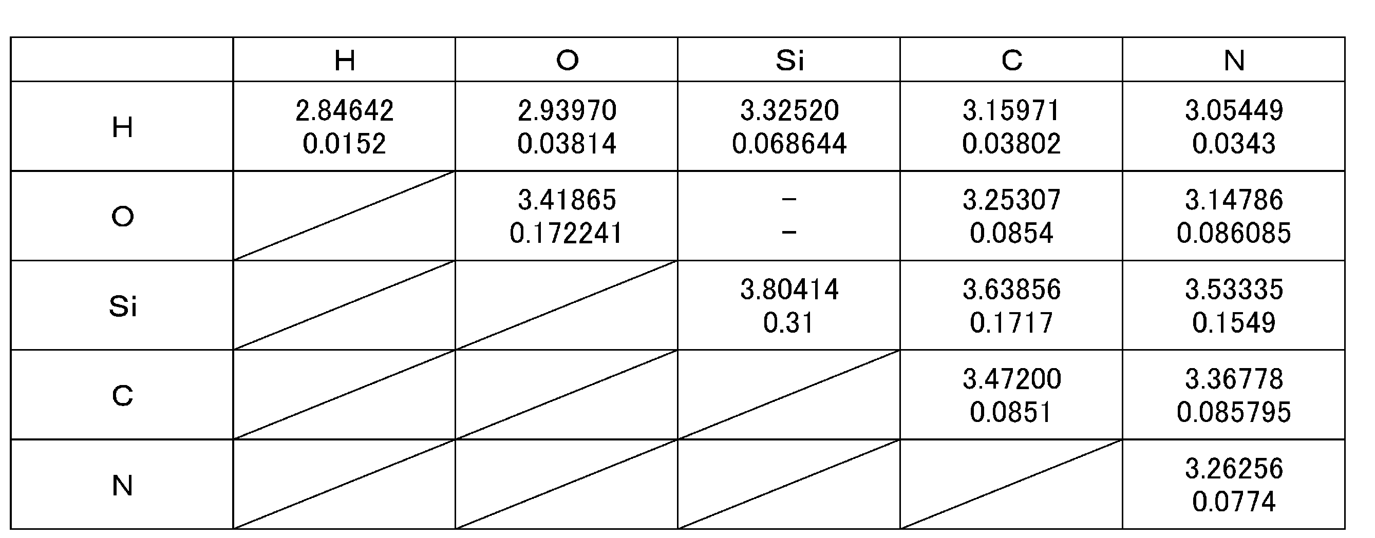
表2に電荷の設定値を示す。ここで各原子に付与した番号は図4(b)に示す。
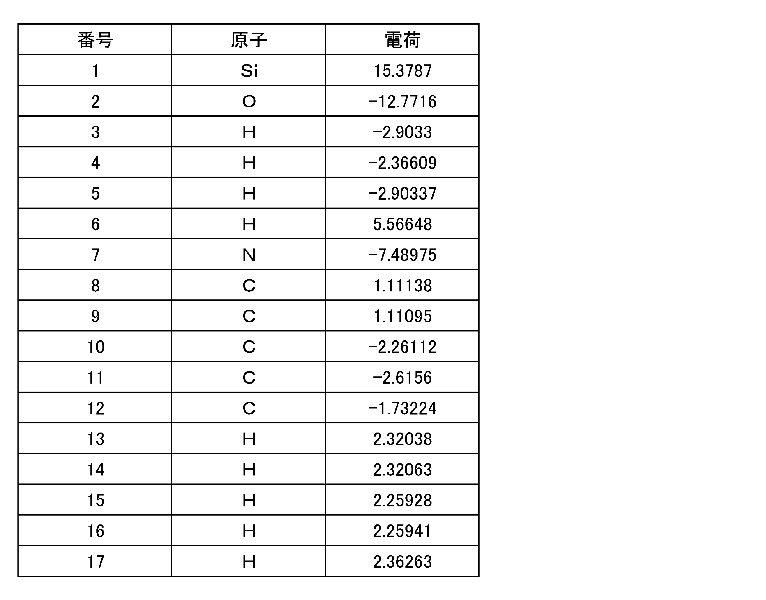
表3に補正したLJポテンシャル(C)のパラメーターを表3に示す。各原子間におけるLJポテンシャル(C)の基準長σ0は表1上段に示したLJポテンシャル(A)と共通である。図4(a)で丸印を付けた原子間、つまり、表3に示した番号の原子間の組み合わせに限りLJポテンシャル(C)のパラメーターεを表1下段に示した値から表3に示した値に変更して計算した。ここで各原子に付与した番号は図4(b)に示す。
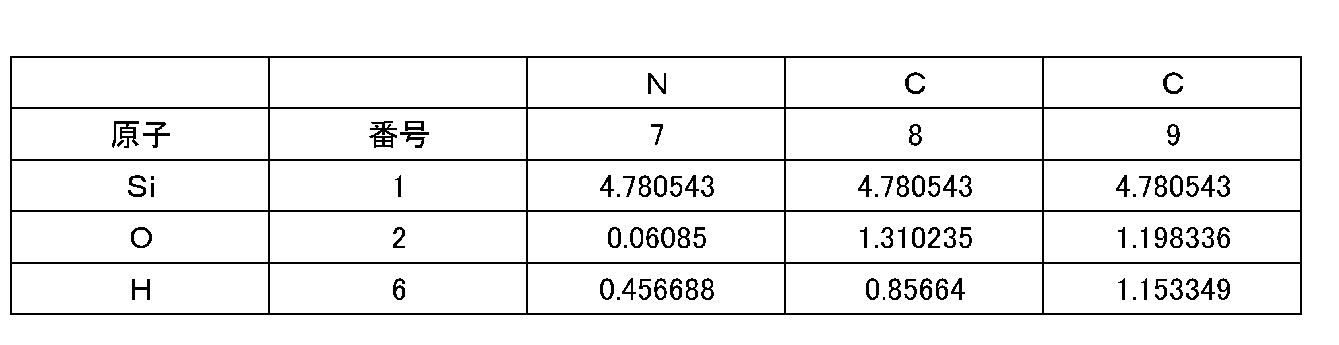
表4に実施例1に示した補正したLJポテンシャル(C)の算出に要した計算時間と、従来技術であるポテンシャル(A)の算出に要した計算時間を表4に示す。表4において、モノマー同士について140,000ステップ計算するのに要した計算時間を項別に秒単位で示したものである。
(計算精度の評価)
計算の精度はモノマー同士の単純な系におけるポテンシャル(A)と(C)の計算結果の一致度合いによって評価した。
計算の精度はモノマー同士の単純な系におけるポテンシャル(A)と(C)の計算結果の一致度合いによって評価した。
(計算速度の評価)
所定ステップ数の計算に要する計算時間により計算速度を評価した。
所定ステップ数の計算に要する計算時間により計算速度を評価した。
モデル分子に対する実施例1である補正したLJポテンシャル(C)と従来技術であるポテンシャル(A)の計算速度を比べると、実施例1の計算速度は合計時間で4.7倍速いことがわかる。LJポテンシャル項と電荷項の合計計算時間を比較すると、実施例1の計算速度は従来技術より45倍高速になっており、ここが両者の速度差の主要因であることがわかる。補正したLJポテンシャル(C)において、電荷の効果を含めたLJポテンシャル項の計算に要する時間が、従来技術におけるLJポテンシャルのみの計算時間と同程度で計算されるためである。一方、従来技術であるポテンシャル(A)では電荷項の計算にさらに多くの時間を費やさねばならないため、計算速度が著しく遅くなる。
なお、実施例1に示した計算要素が1分子同士のモデル分子では計算速度の量的な対比ができたが、分子数を20倍にした系や高分子モデルを想定した系では、設定時間内に従来技術であるポテンシャル(A)は計算収束せず、計算速度を量的に比較することができなかった。実施例である補正したLJポテンシャル(C)においては、通常のLJポテンシャル計算に要する計算時間例えば8時間で十分に計算が収束した。
分子の構成要素数が1分子同士のモデル分子と比べて4000倍(ポリマーを20分子の場合)であることから、30倍程度計算速度が高速化していたと推定される。これは、計算要素数が大きい系において特に電荷項の計算にてしきい値(カットオフ距離)を設定できたため、計算対象がしきい値内の構成要素のみに限定でき、計算量を圧倒的に縮減できたからであり、計算規模が大きくなるほどしきい値の有無で計算量の差が指数的に増大するため、計算速度の差は指数的に大きくなり、実施例では計算可能、従来技術では計算不能という結果の質的な差異に繋がったものと考察される。
分子の構成要素数が1分子同士のモデル分子と比べて4000倍(ポリマーを20分子の場合)であることから、30倍程度計算速度が高速化していたと推定される。これは、計算要素数が大きい系において特に電荷項の計算にてしきい値(カットオフ距離)を設定できたため、計算対象がしきい値内の構成要素のみに限定でき、計算量を圧倒的に縮減できたからであり、計算規模が大きくなるほどしきい値の有無で計算量の差が指数的に増大するため、計算速度の差は指数的に大きくなり、実施例では計算可能、従来技術では計算不能という結果の質的な差異に繋がったものと考察される。
1 システム
2 コンピュータ
3 コンピュータ本体
4 入力装置(キーボード)
5 ディスプレイ
6 記録媒体駆動ユニット
7 記録媒体
P1 N-O原子間の非結合相互作用(LJ)ポテンシャル曲線
P2 N-O原子間の静電相互作用(クーロン)ポテンシャル曲線
P3 N-Si原子間の非結合相互作用(LJ)ポテンシャル曲線
P4 N-Si原子間の静電相互作用(クーロン)ポテンシャル曲線
P5 モデル分子A1-A2間の非結合相互作用ポテンシャル(A)曲線
P6 モデル分子A1-A2間の非結合相互作用(LJ)ポテンシャル(B)曲線
P7 モデル分子A1-A2間の静電相互作用(クーロン)ポテンシャル曲線
P8 モデル分子C1-C2間のLJポテンシャル補正項(C)曲線
2 コンピュータ
3 コンピュータ本体
4 入力装置(キーボード)
5 ディスプレイ
6 記録媒体駆動ユニット
7 記録媒体
P1 N-O原子間の非結合相互作用(LJ)ポテンシャル曲線
P2 N-O原子間の静電相互作用(クーロン)ポテンシャル曲線
P3 N-Si原子間の非結合相互作用(LJ)ポテンシャル曲線
P4 N-Si原子間の静電相互作用(クーロン)ポテンシャル曲線
P5 モデル分子A1-A2間の非結合相互作用ポテンシャル(A)曲線
P6 モデル分子A1-A2間の非結合相互作用(LJ)ポテンシャル(B)曲線
P7 モデル分子A1-A2間の静電相互作用(クーロン)ポテンシャル曲線
P8 モデル分子C1-C2間のLJポテンシャル補正項(C)曲線
Claims (3)
- 計算機を用いて分子動力学法によるシミュレーションを行うことで非結合相互作用ポテンシャルを求める計算手法において、
系内に存在する複数の分子のうちから2分子を選択しそれらをモデル分子とする工程と、
前記モデル分子の電荷を求めて、求まった電荷をそれぞれの分子に付与する工程と、
前記モデル分子を系内で3次元的に動かすことで非結合相互作用ポテンシャル(A)を算出する工程と、
静電相互作用を0として、前記モデル分子を系内で3次元的に動かすことで非クーロン力作用下の非結合相互作用ポテンシャル(B)を算出する工程と、
算出された前記非結合相互作用ポテンシャル(A)と前記非クーロン力作用下での非結合相互作用ポテンシャル(B)とを比較演算することで、Lennard-Jonesポテンシャル(C)を算出する工程と、
を有することを特徴とする非結合相互作用ポテンシャルの計算手法。 - 請求項1に記載の前記Lennard-Jonesポテンシャルの補正項(C)を基に、系内に存在する分子に適用する工程を有することを特徴とする分子間相互作用計算手法。
- 前記モデル分子は高分子からなる計算単位をいずれか一つを含むことを特徴とする請求項1又は2に記載の計算手法。
Applications Claiming Priority (2)
| Application Number | Priority Date | Filing Date | Title |
|---|---|---|---|
| JP2010119880A JP2011248541A (ja) | 2010-05-25 | 2010-05-25 | 分子間力のシミュレーション手法 |
| JP2010-119880 | 2010-05-25 |
Publications (1)
| Publication Number | Publication Date |
|---|---|
| WO2011148639A1 true WO2011148639A1 (ja) | 2011-12-01 |
Family
ID=45003638
Family Applications (1)
| Application Number | Title | Priority Date | Filing Date |
|---|---|---|---|
| PCT/JP2011/002927 Ceased WO2011148639A1 (ja) | 2010-05-25 | 2011-05-25 | 分子間力のシミュレーション手法 |
Country Status (2)
| Country | Link |
|---|---|
| JP (1) | JP2011248541A (ja) |
| WO (1) | WO2011148639A1 (ja) |
Cited By (6)
| Publication number | Priority date | Publication date | Assignee | Title |
|---|---|---|---|---|
| JP2013238535A (ja) * | 2012-05-16 | 2013-11-28 | Sumitomo Rubber Ind Ltd | 高分子材料のシミュレーション方法 |
| JP2014206915A (ja) * | 2013-04-15 | 2014-10-30 | 住友ゴム工業株式会社 | 高分子材料のシミュレーション方法 |
| WO2014198080A1 (zh) * | 2013-06-09 | 2014-12-18 | Zhang Shunxin | 一种分子间相互作用力的分析方法 |
| EP2704048A3 (en) * | 2012-08-31 | 2018-03-21 | Sumitomo Rubber Industries, Ltd. | Method for simulating polymer material |
| CN109270590A (zh) * | 2018-10-22 | 2019-01-25 | 中国地震局地壳应力研究所 | 非均匀椭球地球地震和地表载荷库伦应力计算方法 |
| CN110459272A (zh) * | 2019-08-19 | 2019-11-15 | 中南大学 | 一种基于力匹配的铝电解熔盐体系力场拟合方法 |
Families Citing this family (4)
| Publication number | Priority date | Publication date | Assignee | Title |
|---|---|---|---|---|
| JP5592921B2 (ja) * | 2012-06-21 | 2014-09-17 | 住友ゴム工業株式会社 | 高分子材料のシミュレーション方法 |
| JP5530480B2 (ja) * | 2012-07-05 | 2014-06-25 | 住友ゴム工業株式会社 | 高分子材料のシミュレーション方法 |
| JP7658079B2 (ja) * | 2020-11-26 | 2025-04-08 | 住友ゴム工業株式会社 | 高分子材料の相互作用の解析方法 |
| JP7690824B2 (ja) * | 2021-09-07 | 2025-06-11 | 住友ゴム工業株式会社 | 高分子材料のシミュレーション方法 |
Citations (2)
| Publication number | Priority date | Publication date | Assignee | Title |
|---|---|---|---|---|
| JP2005208930A (ja) * | 2004-01-22 | 2005-08-04 | Sumitomo Rubber Ind Ltd | フィラー間相互作用のシミュレーション方法 |
| JP2007149075A (ja) * | 2005-10-27 | 2007-06-14 | Toray Ind Inc | 粗視化分子シミュレーション用点電荷決定方法 |
-
2010
- 2010-05-25 JP JP2010119880A patent/JP2011248541A/ja active Pending
-
2011
- 2011-05-25 WO PCT/JP2011/002927 patent/WO2011148639A1/ja not_active Ceased
Patent Citations (2)
| Publication number | Priority date | Publication date | Assignee | Title |
|---|---|---|---|---|
| JP2005208930A (ja) * | 2004-01-22 | 2005-08-04 | Sumitomo Rubber Ind Ltd | フィラー間相互作用のシミュレーション方法 |
| JP2007149075A (ja) * | 2005-10-27 | 2007-06-14 | Toray Ind Inc | 粗視化分子シミュレーション用点電荷決定方法 |
Cited By (8)
| Publication number | Priority date | Publication date | Assignee | Title |
|---|---|---|---|---|
| JP2013238535A (ja) * | 2012-05-16 | 2013-11-28 | Sumitomo Rubber Ind Ltd | 高分子材料のシミュレーション方法 |
| EP2704048A3 (en) * | 2012-08-31 | 2018-03-21 | Sumitomo Rubber Industries, Ltd. | Method for simulating polymer material |
| JP2014206915A (ja) * | 2013-04-15 | 2014-10-30 | 住友ゴム工業株式会社 | 高分子材料のシミュレーション方法 |
| WO2014198080A1 (zh) * | 2013-06-09 | 2014-12-18 | Zhang Shunxin | 一种分子间相互作用力的分析方法 |
| CN104240563A (zh) * | 2013-06-09 | 2014-12-24 | 张顺信 | 一种分子间相互作用力的分析方法 |
| CN109270590A (zh) * | 2018-10-22 | 2019-01-25 | 中国地震局地壳应力研究所 | 非均匀椭球地球地震和地表载荷库伦应力计算方法 |
| CN110459272A (zh) * | 2019-08-19 | 2019-11-15 | 中南大学 | 一种基于力匹配的铝电解熔盐体系力场拟合方法 |
| CN110459272B (zh) * | 2019-08-19 | 2023-03-31 | 中南大学 | 一种基于力匹配的铝电解熔盐体系力场拟合方法 |
Also Published As
| Publication number | Publication date |
|---|---|
| JP2011248541A (ja) | 2011-12-08 |
Similar Documents
| Publication | Publication Date | Title |
|---|---|---|
| WO2011148639A1 (ja) | 分子間力のシミュレーション手法 | |
| JP5548180B2 (ja) | 高分子材料のシミュレーション方法 | |
| Zhang et al. | Modelling large-scale landslide using a GPU-accelerated 3D MPM with an efficient terrain contact algorithm | |
| Abbas et al. | Micromechanical modeling of the viscoelastic behavior of asphalt mixtures using the discrete-element method | |
| Li et al. | Meshfree particle methods | |
| Gates et al. | Computational materials: multi-scale modeling and simulation of nanostructured materials | |
| JP4594043B2 (ja) | ゴム材料のシミュレーション方法 | |
| JP2012177609A (ja) | 高分子材料のモデル作成方法 | |
| US9081921B2 (en) | Method for simulating rubber compound | |
| Hou et al. | Study on the microscopic friction between tire and asphalt pavement based on molecular dynamics simulation | |
| Clayton et al. | Nanoparticle orientation distribution analysis and design for polymeric piezoresistive sensors | |
| US20140309975A1 (en) | Analysis device and simulation method | |
| Falk et al. | Multiscale simulation to determine rubber friction on asphalt surfaces | |
| Yan et al. | A multiscale computational framework for the analysis of graphene involving geometrical and material nonlinearities | |
| Yang et al. | Molecular dynamics simulation based size and rate dependent constitutive model of polystyrene thin films | |
| JP5592921B2 (ja) | 高分子材料のシミュレーション方法 | |
| Berry et al. | Lees-Edwards boundary conditions for the multi-sphere discrete element method | |
| JP6244773B2 (ja) | 複合材料の解析用モデルの作成方法、複合材料の解析用コンピュータプログラム、複合材料のシミュレーション方法及び複合材料のシミュレーション用コンピュータプログラム | |
| Zhao et al. | Simulation of elastic and fatigue properties of epoxy/SiO2 particle composites through molecular dynamics | |
| JP5782604B2 (ja) | 情報処理装置及びプログラム | |
| JP6746971B2 (ja) | 複合材料の解析方法及び複合材料の解析用コンピュータプログラム | |
| JP2010287042A (ja) | 回転体のシミュレーション方法、装置及びプログラム | |
| WO2016013640A1 (ja) | 特定物質の解析用モデルの作成方法、特定物質の解析用モデルの作成用コンピュータプログラム、特定物質のシミュレーション方法及び特定物質のシミュレーション用コンピュータプログラム | |
| JP2020085692A (ja) | ゴム材料のシミュレーション方法 | |
| JP2007149075A (ja) | 粗視化分子シミュレーション用点電荷決定方法 |
Legal Events
| Date | Code | Title | Description |
|---|---|---|---|
| 121 | Ep: the epo has been informed by wipo that ep was designated in this application |
Ref document number: 11786342 Country of ref document: EP Kind code of ref document: A1 |
|
| NENP | Non-entry into the national phase |
Ref country code: DE |
|
| 122 | Ep: pct application non-entry in european phase |
Ref document number: 11786342 Country of ref document: EP Kind code of ref document: A1 |