WO2011046212A1 - 画像解析方法および画像解析装置 - Google Patents
画像解析方法および画像解析装置 Download PDFInfo
- Publication number
- WO2011046212A1 WO2011046212A1 PCT/JP2010/068192 JP2010068192W WO2011046212A1 WO 2011046212 A1 WO2011046212 A1 WO 2011046212A1 JP 2010068192 W JP2010068192 W JP 2010068192W WO 2011046212 A1 WO2011046212 A1 WO 2011046212A1
- Authority
- WO
- WIPO (PCT)
- Prior art keywords
- image
- value
- analysis
- data
- frame
- Prior art date
- Legal status (The legal status is an assumption and is not a legal conclusion. Google has not performed a legal analysis and makes no representation as to the accuracy of the status listed.)
- Ceased
Links
Images








Classifications
-
- G—PHYSICS
- G06—COMPUTING OR CALCULATING; COUNTING
- G06T—IMAGE DATA PROCESSING OR GENERATION, IN GENERAL
- G06T7/00—Image analysis
- G06T7/97—Determining parameters from multiple pictures
-
- G—PHYSICS
- G01—MEASURING; TESTING
- G01N—INVESTIGATING OR ANALYSING MATERIALS BY DETERMINING THEIR CHEMICAL OR PHYSICAL PROPERTIES
- G01N21/00—Investigating or analysing materials by the use of optical means, i.e. using sub-millimetre waves, infrared, visible or ultraviolet light
- G01N21/62—Systems in which the material investigated is excited whereby it emits light or causes a change in wavelength of the incident light
- G01N21/63—Systems in which the material investigated is excited whereby it emits light or causes a change in wavelength of the incident light optically excited
- G01N21/64—Fluorescence; Phosphorescence
- G01N21/645—Specially adapted constructive features of fluorimeters
- G01N21/6456—Spatial resolved fluorescence measurements; Imaging
- G01N21/6458—Fluorescence microscopy
-
- G—PHYSICS
- G06—COMPUTING OR CALCULATING; COUNTING
- G06T—IMAGE DATA PROCESSING OR GENERATION, IN GENERAL
- G06T2207/00—Indexing scheme for image analysis or image enhancement
- G06T2207/10—Image acquisition modality
- G06T2207/10056—Microscopic image
-
- G—PHYSICS
- G06—COMPUTING OR CALCULATING; COUNTING
- G06T—IMAGE DATA PROCESSING OR GENERATION, IN GENERAL
- G06T2207/00—Indexing scheme for image analysis or image enhancement
- G06T2207/10—Image acquisition modality
- G06T2207/10064—Fluorescence image
-
- G—PHYSICS
- G06—COMPUTING OR CALCULATING; COUNTING
- G06T—IMAGE DATA PROCESSING OR GENERATION, IN GENERAL
- G06T2207/00—Indexing scheme for image analysis or image enhancement
- G06T2207/30—Subject of image; Context of image processing
- G06T2207/30004—Biomedical image processing
- G06T2207/30024—Cell structures in vitro; Tissue sections in vitro
Definitions
- the present invention relates to an image analysis method and an image analysis apparatus.
- Non-Patent Documents 1 and 2 have been proposed as Raster Image Correlation Spectroscopy (RICS).
- RANS Raster Image Correlation Spectroscopy
- a fluorescence image composed of a raster scan image of one frame or more is acquired.
- an area of interest is determined in the sample to be image-analyzed, and the area is repeatedly scanned by the raster scanning method to obtain an image composed of a plurality of frames of fluorescence intensity.
- the fluorescence intensity in the frame is expressed as data in pixel units.
- Pieces of pixel data have different acquisition times and acquisition positions, so that the acquisition times and acquisition positions corresponding to the data are different.
- correlation characteristics due to molecular fluctuations can be obtained by performing spatial correlation analysis using the data of these pixels.
- the diffusion constant and the number of molecules can be obtained from the correlation characteristics of the molecules.
- the pixel time and line time are determined by the scanning speed and cannot be changed after the image is acquired. For this reason, in order to appropriately obtain the molecular diffusion constant and the like, it is necessary to estimate an appropriate pixel time and line time before image acquisition. However, since the molecular diffusion time of most samples is unknown, it is difficult to estimate the pixel time and line time settings in advance.
- An object of the present invention is to provide an RICS image analysis method capable of performing spatial correlation analysis with high accuracy even in an analysis region having a small number of pixels and extending an observable diffusion time.
- An image analysis method includes: an image acquisition step of acquiring a plurality of frames of images each including a plurality of pixels in which pixel data of each image is acquired in time series; An analysis region setting step for setting an analysis region for the image, an image selection step for selecting a selection image of two or more frames to be used for analysis from the images of the plurality of frames, and an analysis region in the same image of the selection image
- An analysis region setting step for setting an analysis region for the image
- an image selection step for selecting a selection image of two or more frames to be used for analysis from the images of the plurality of frames, and an analysis region in the same image of the selection image
- the product-sum calculation of data pairs of two pixels having the same acquisition time interval is performed for all of the selected images, and two pixels having the same acquisition time interval in the analysis region of two different images of the selected image And calculating a correlation value by performing a product-sum calculation of the data pairs.
- a RICS image analysis method capable of performing spatial correlation analysis with high accuracy even in an analysis region having a small number of pixels and extending an observable diffusion time.
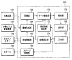
- FIG. 1 schematically shows an image analysis device according to an embodiment of the invention.
- the functional block of the control part shown by FIG. 1 is shown.
- 3 is a flowchart of image analysis according to an embodiment of the present invention.
- frame acquired in time series used for an image analysis is shown.
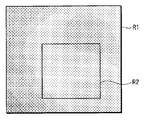
- the observation area and the analysis area are shown.
- frame classified into the several group is shown typically.
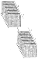
- An image of a plurality of frames divided into a plurality of blocks is schematically shown.
- the product-sum calculation of the correlation calculation in the image of the ⁇ frame is schematically shown.
- the sum of products calculation of the correlation calculation between the images of the ⁇ frame and the ( ⁇ + 1) frame is schematically shown.
- the product-sum calculation of the correlation calculation between the images of the ⁇ frame and the ( ⁇ + 2) frame is schematically shown.
- the sum of products calculation of the correlation calculation between the images of the ⁇ frame and the p frame is schematically shown.
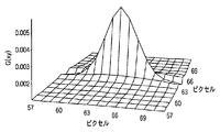
- the variables ⁇ , ⁇ , ⁇ in the equations (1) to (4) and the frame used for the calculation are shown. It is the image which showed the calculation result of the spatial correlation value by RICS with respect to a small molecule
- numerator is shown. It is the image which showed the calculation result of the spatial correlation value by RICS with respect to a big molecule
- the fitting result of the spatial correlation value by RICS for a large molecule is shown.
- the result of comparing the diffusion constant (D) of the EGFP solution while changing the ROI size in the analysis region is shown.
- FIG. 1 schematically shows an image analysis apparatus according to an embodiment of the present invention.
- This image analysis apparatus is configured based on a scanning confocal optical microscope for fluorescence observation of a sample.
- the image analysis apparatus 100 is necessary for image analysis, a light irradiation unit 110 that irradiates the sample S with excitation light, a light detection unit 130 that detects light emitted from a measurement point in the sample S, and the like. And a sample stage 190 that supports the sample S.
- the sample S is accommodated in a sample container such as a microplate or a slide glass, and is placed on the sample stage 190.
- the sample stage 190 supports the sample S so as to be movable in the lateral direction (xy direction) and the height direction (z direction) with respect to the light irradiation unit 110 and the light detection unit 130.
- the sample stage 190 includes three stepping motors whose output axes are orthogonal to each other, and the sample S can be moved in the xyz direction by these stepping motors.
- the image analysis apparatus 100 is a multiple light irradiation / multiple light detection type.
- the light irradiation unit 110 includes an n-channel light source system 111, and the light detection unit 130 correspondingly includes an n-channel detection system 131.
- Each of the n-channel detection systems 131 detects fluorescence generated by the excitation light emitted from the n-channel light source system 111.
- the n channel includes channel 1, channel 2,... Channel n. The channel differs depending on the type of excitation light.
- the n-channel light source system 111 of the light irradiation unit 110 includes light sources 112a, ..., 112n, collimating lenses 114a, ..., 114n, and dichroic mirrors 116a, ..., 116n.
- the light sources 112a,..., 112n emit excitation light for exciting the fluorescent dye contained in the sample S to emit light (fluorescence) from the sample S.
- the wavelengths of the excitation light emitted from the light sources 112a,..., 112n are different from each other corresponding to the type of fluorescent dye contained in the sample S.
- the light sources 112a,..., 112n are constituted by, for example, laser light sources having an oscillation wavelength suitable for the fluorescent dye in the sample S.
- the collimating lenses 114a,..., 114n collimate the excitation light emitted from the light sources 112a,.
- the dichroic mirrors 116a,..., 116n reflect the excitation light that has passed through the collimating lenses 114a,.
- Each of the dichroic mirrors 116a,..., 116n transmits the excitation light incident from above in FIG. 1 and reflects the excitation light incident from the right side in FIG.
- the excitation lights having different wavelengths respectively emitted from the light sources 112a,..., 112n are combined into one beam after passing through the dichroic mirror 116a.
- the dichroic mirror 116n does not need to transmit the excitation light, and may be changed to a simple mirror.
- the light irradiation unit 110 further includes a dichroic mirror 122, a galvano mirror 124, an objective lens 126, and an objective lens driving mechanism 128.
- the dichroic mirror 122 reflects the excitation light from the light source system 111 toward the galvanometer mirror 124 and transmits the fluorescence emitted from the sample S.
- the galvanometer mirror 124 reflects the excitation light toward the objective lens 126 and changes the reflection direction thereof.
- the objective lens 126 converges the excitation light and irradiates the measurement point in the sample S, and takes in the light from the measurement point in the sample S.
- An objective lens 126 having a large NA (numerical aperture) is used to form a minute confocal region (measurement point).
- the confocal region thus obtained has a substantially cylindrical shape with a diameter of about 0.6 ⁇ m and a length of about 2 ⁇ m.
- the galvanometer mirror 124 constitutes an xy scanning mechanism that scans measurement points in the xy direction.
- the xy scanning mechanism may be configured using an acousto-optic modulation element (AOM), a polygon mirror, a hologram scanner, or the like in addition to using a galvano mirror.
- AOM acousto-optic modulation element
- the objective lens driving mechanism 128 moves the objective lens 126 along the optical axis. Thereby, the measurement point is moved in the z direction. That is, the objective lens driving mechanism 128 constitutes a z scanning mechanism that scans the measurement point in the z direction.
- the light detection unit 130 shares the objective lens 126, the galvano mirror 124, and the dichroic mirror 122 with the light irradiation unit 110.
- the light detection unit 130 further includes a converging lens 132, a pinhole 134, and a collimating lens 136.
- the converging lens 132 converges the light transmitted through the dichroic mirror 122.
- the pinhole 134 is disposed at the focal point of the converging lens 132. That is, the pinhole 134 is in a conjugate position with respect to the measurement point in the sample S, and selectively allows only light from the measurement point to pass through.
- the collimating lens 136 collimates the light that has passed through the pinhole 134.
- the light that has passed through the collimator lens 136 enters the n-channel detection system 131.
- the n-channel detection system 131 includes dichroic mirrors 138a, ..., 138n, fluorescent filters 140a, ..., 140n, and photodetectors 142a, ..., 142n.
- the dichroic mirrors 138a,..., 138n selectively reflect light having a wavelength in the vicinity of the fluorescent wavelength region generated from the sample S by the excitation light from the light sources 112a,.
- the dichroic mirror 138n does not need to transmit light, and may be changed to a simple mirror.
- the fluorescence filters 140a,..., 140n block the light having an undesired wavelength component from the light reflected by the dichroic mirrors 138a,..., 138n, respectively, and are generated by the excitation light from the light sources 112a,. Only the fluorescence is selectively transmitted.
- the fluorescence transmitted through the fluorescent filters 140a,..., 140n is incident on the photodetectors 142a,.
- the photodetectors 142a,..., 142n output signals corresponding to the intensity of incident light. That is, the photodetectors 142a,..., 142n output fluorescence intensity signals from the measurement points in the sample S.
- the control unit 160 is constituted by a personal computer, for example.
- the control unit 160 acquires, stores, and displays the fluorescence image of the observation region of the sample S, waits for input of the number of frames (number of frames) of the acquired fluorescence image and the setting of the analysis region, image analysis (calculation of correlation value), diffusion time Etc. are estimated.
- the control unit 160 controls the galvano mirror 124 that is an xy scanning mechanism, the objective lens driving mechanism 128 that is a z scanning mechanism, the sample stage 190, and the like.
- the control unit 160 includes a scan control unit 162, an image forming unit 164, a storage unit 166, a display unit 168, an input unit 170, an analysis region setting unit 172, an image selection unit 174, and a data extraction unit 176.
- An analysis unit 178 and a stage control unit 180 are included.
- the scanning control unit 162, the image forming unit 164, the storage unit 166, the stage control unit 180, the galvano mirror 124, the objective lens driving mechanism 128, the sample stage 190, and the photodetector 142 constitute an image acquisition unit.
- the data extraction unit 176 and the analysis unit 178 constitute an arithmetic unit.
- the scanning control unit 162 controls the galvanometer mirror 124 so as to raster scan the irradiation position of the excitation light with respect to the sample S when acquiring the fluorescence image of the sample S.
- the scanning control unit 162 also controls the objective lens driving mechanism 128 so that the irradiation position of the excitation light is z-scanned with respect to the sample S if necessary.
- the image forming unit 164 forms a fluorescent image of the sample S from the information on the irradiation position of the excitation light input from the scanning control unit 162 and the output signals of the photodetectors 142a,. Thereby, a fluorescence image is acquired.
- the storage unit 166 sequentially stores the fluorescent images formed by the image forming unit 164.
- the display unit 168 displays the fluorescence image of the sample S and the analysis result.
- the input unit 170 includes, for example, a mouse and a keyboard, and constitutes a GUI in cooperation with the display unit 168. This GUI is used for setting the number of acquired frames, the observation area, and the analysis area.
- the stage control unit 180 controls the sample stage 190 according to the input information from the input unit 170 in order to set an observation region, for example.
- the analysis area setting unit 172 sets an analysis area according to the input information from the input unit 170.
- the image selection unit 174 selects fluorescent images of two or more frames used for analysis according to the input information from the input unit 170.
- the data extraction unit 176 extracts necessary data from the fluorescence image stored in the storage unit 166 based on the input information from the analysis region setting unit 172 and the image selection unit 174. Necessary data includes two pairs of data of two pixels having the same acquisition time interval in the analysis region of the same image of the fluorescence image selected by the image selection unit 174 and two different images selected by the image selection unit 174. A data pair of two pixels having the same acquisition time interval in the analysis region of one image.
- the data included in the plurality of data pairs may be, for example, data of all pixels or data of some pixels of all fluorescent images stored in the storage unit 166 or stored in the storage unit 166. The data of all pixels or the data of some pixels of a part of the fluorescent image that is being recorded may be used. Data extraction is performed according to equations (1) to (4) described later.
- the analysis unit 178 calculates a correlation value described later on the data extracted by the data extraction unit 176.
- excitation light emitted from light sources 112a,..., 112n passes through collimating lenses 114a,..., 114n, dichroic mirrors 116a,.
- the measurement point is irradiated.
- the measurement point irradiated with the excitation light is raster scanned in the xy direction by the galvanometer mirror 124. If necessary, z scanning is performed by the objective lens driving mechanism 128.
- the sample S that has received the excitation light emits fluorescence from the measurement point.
- Light from the sample S (including undesired reflected light in addition to fluorescence) reaches the pinhole 134 through the objective lens 126, the galvanometer mirror 124, the dichroic mirror 122, and the converging lens 132.
- the pinhole 134 Since the pinhole 134 is at a position conjugate with the measurement point, only light from the measurement point in the sample S passes through the pinhole 134.
- the light that has passed through the pinhole 134 that is, the light from the measurement point in the sample S, enters the n-channel detection system 131 through the collimator lens 136.
- the light incident on the n-channel detection system 131 is separated (that is, spectrally separated) by the dichroic mirrors 138a,..., 138n, and unwanted components are removed by the fluorescent filters 140a,. .
- the fluorescent filters 140a As a result, only the fluorescence generated by the excitation light from the light sources 112a,..., 112n enters the photodetectors 142a,.
- Each of the photodetectors 142a,..., 142n outputs incident light, that is, a fluorescence intensity signal indicating the intensity of fluorescence emitted from a measurement point in the sample S.
- This fluorescence intensity signal is input to the image forming unit 164.
- the image forming unit 164 processes the input fluorescence intensity signal in synchronism with position information in the xy direction (and z direction) for each raster scan (and z scan), and the focal plane in the sample S
- a fluorescent image of one frame (a flat surface or a curved surface where the measurement point has moved) is formed.
- the formed fluorescent image is stored in the storage unit 166.
- the series of operations described here is repeated for the set number of frames to be acquired, and a fluorescence image having the set number of frames is acquired.
- Each fluorescent image is composed of a plurality of pixels from which pixel data is acquired in time series.
- the fluorescent image stored in the storage unit 166 is processed as necessary and displayed on the display unit 168.
- the spatial correlation calculation formula used in this embodiment is an extension of the conventional spatial correlation calculation formula so that a sufficient number of data and a sufficient delay time can be obtained.
- Equation (1) represents a spatial autocorrelation calculation formula used for analysis of RICS used in the present embodiment. Equation (1) is an example of an autocorrelation calculation equation for channel 1.
- G sa is the RICS spatial autocorrelation value
- I 1 ⁇ is the fluorescence intensity data (pixel data) of the ⁇ frame of channel 1
- I 1 ( ⁇ + ⁇ ) is the fluorescence intensity data of the ( ⁇ + ⁇ ) frame of channel 1 (Pixel data)
- x and y are the spatial coordinates of the measurement point
- ⁇ and ⁇ are the amount of change in the spatial coordinate from the measurement point
- M 1 ⁇ 1 ( ⁇ + ⁇ ) is the product sum of the ⁇ frame of channel 1 and the ( ⁇ + ⁇ ) frame of channel 1 number of calculations
- a 1 is an average value.
- ⁇ and ( ⁇ + ⁇ ) are both parameters indicating the frame subject to product-sum calculation.
- ⁇ and ⁇ are for selecting a fluorescence image to be used for correlation analysis with respect to a plurality of frames of fluorescence images.
- ⁇ indicates one frame to be subjected to product-sum calculation, and ⁇ is a parameter introduced for time extension, and indicates a delay in the number of frames with respect to ⁇ .
- q represents the total number of frames used for spatial correlation calculation.
- p represents the number of frames that determines the maximum delay time in the spatial correlation calculation. The maximum possible value of p is q-1.
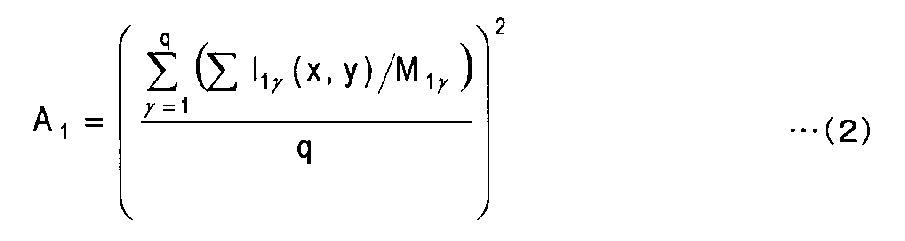
- Mean value A 1 for example is expressed by the following equation (2).
- M 1 ⁇ is the number of data used for the calculation of the ⁇ -th frame of channel 1.
- Equation for calculating the average value A 1 is not limited to Equation (2).
- Mean value A 1 may be calculated using any formula other known.
- Equation (3) represents a spatial cross-correlation calculation formula used for RICS analysis used in this embodiment. Equation (3) is an example of a cross-correlation calculation formula for channel 1 and channel 2.
- G sc is the RICS spatial cross-correlation value
- I 1 ⁇ is the fluorescence intensity data (pixel data) of the ⁇ frame of channel 1
- I 2 ( ⁇ + ⁇ ) is the fluorescence intensity data of the ( ⁇ + ⁇ ) frame of channel 2.
- x and y are the spatial coordinates of the measurement point
- ⁇ and ⁇ are the amount of change in the spatial coordinate from the measurement point
- M 1 ⁇ 2 ( ⁇ + ⁇ ) is the product sum calculation of the ⁇ frame of channel 1 and the ( ⁇ + ⁇ ) frame of channel 2 number of, a 2 is an average value.
- ⁇ and ⁇ indicate the delay of the number of frames with respect to one frame of the product-sum calculation target and ⁇ , respectively, as in the equation (1).
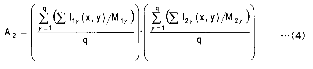
- Mean value A 2 for example is expressed by the following equation (4).
- M 1 ⁇ is the number of data used for calculation of the ⁇ frame of channel 1
- M 2 ⁇ is the number of data used for calculation of the ⁇ frame of channel 2.
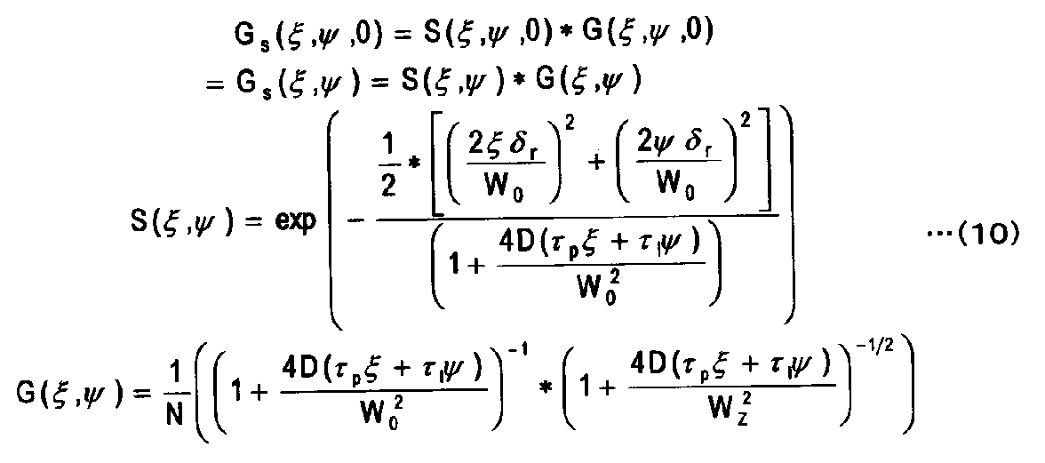
- Equation (5) represents a fitting equation used for analysis of RICS used in the present embodiment.
- G s is the RICS spatial correlation value (spatial autocorrelation value G sa or spatial cross-correlation value G sc ), S is the influence of scanning in the RICS analysis, G is the influence of time delay in the RICS analysis, and D is Diffusion constant, ⁇ r is the pixel size, N is the number of molecules, W 0 is the lateral radius of the excitation laser beam, W Z is the longitudinal radius of the excitation laser beam, ⁇ p is the pixel time, ⁇ l is the line time, ⁇ f is the frame time.
- ⁇ p is a shift in acquisition time between pixels. That is, the pixel time ⁇ p is a time required to acquire data for one pixel.
- ⁇ l is an acquisition time shift (line time) between the first pixel of an arbitrary line and the first pixel of the next line. That is, the line time ⁇ 1 means the time required to scan one line.
- ⁇ f is a shift in acquisition time between the first pixel of an arbitrary frame and the first pixel of the next frame. That is, the frame time ⁇ f means the time required to scan one frame.
- I 1 is the fluorescence intensity data (pixel data) of the same frame of channel 1
- x and y are the spatial coordinates of the measurement point
- ⁇ and ⁇ are the amount of change in the spatial coordinates from the measurement point
- M 11 is This is the number of product-sum calculations in the same frame of channel 1.
- Mean value A 1 is expressed by the following equation (7).
- M 1 is the number of data used for calculation in the same frame of channel 1.
- I 1 is the fluorescence intensity data (pixel data) of the frame used for the calculation of channel 1
- I 2 is the fluorescence intensity data (pixel data) of the frame used for the calculation of channel 2
- x and y are the measurements
- the spatial coordinates of the points, ⁇ , ⁇ are the amount of change in the spatial coordinates from the measurement point
- M 12 is the number of product-sum calculations of data in channel 1 and channel 2.
- Mean value A 2 is expressed by the following equation (9).
- M 1 is the number of data used for calculation in the frame used for calculation of channel 1
- M 2 is the number of data used for calculation in the frame used for calculation of channel 2.
- Step S1 The observation area of the sample S and the number of frames of the fluorescent image to be acquired are set. Fluorescence images of the set number of frames in the set observation area are acquired in time series. The fluorescence image is acquired by the same scanning method for the same observation region. In other words, when one set of scanning is performed from the irradiation of light toward a predetermined direction to the irradiation of light toward the predetermined direction again, at least two sets or more of the analysis region are scanned.
- FIG. 4 schematically shows a plurality of frames of fluorescent images used for image analysis.
- the plurality of frames of fluorescent images used for image analysis may be all or some of the images acquired in step S1.
- a plurality of frames of fluorescent images used for image analysis are simply referred to as a plurality of frames of fluorescent images.
- F k represents the fluorescence image of the k-th frame in one channel.
- Each fluorescent image is composed of a plurality of pixels from which pixel data is acquired in time series. Pixel data is, for example, fluorescence intensity obtained from a two-dimensional or three-dimensional observation region.
- Step S2 As shown in FIG. 5, a region (analysis region) R2 to be analyzed is set with respect to a region (observation region) R1 of the fluorescence image used for image analysis.
- the analysis region R2 is not limited to a part of the observation region R1, and may coincide with the observation region R1.
- the analysis area R2 is set as an observation area R1, that is, a scanning area in step S1 by default in terms of application. This step is not necessary when analyzing the entire observation region R1.
- Step S3 A plurality of frames of fluorescent images are classified based on data information changes. For example, the segment values of the analysis region R2 of the plurality of frames of fluorescence images are calculated, and the plurality of frames of fluorescence images are classified into a plurality of groups based on the calculated segment values.
- the segment value is, for example, a statistical value of pixel data in the analysis region R2, and is any one of a maximum value, a minimum value, an average value, a relative difference, and a relative ratio of pixel data in the analysis region R2.
- Pixel data is, for example, fluorescence intensity obtained from a two-dimensional or three-dimensional observation region.
- the relative difference is, for example, a difference between a maximum value and a minimum value.
- FIG. 6 schematically shows images of analysis regions of fluorescent images of a plurality of frames classified into a plurality of groups.
- Fa k represents the image of the analysis area of the k-th frame of the fluorescent image.
- D a , D b , D c , D d , D e , and D f represent segment values in the analysis region of the fluorescence image.
- Fa 1 , Fa 2 , Fa 79 , and Fa 80 are classified into the same group
- Fa 3 , Fa 74 , and Fa 75 are classified into the same group
- Fa 4 , Fa 71 , Fa 72 , Fa 73 Are classified into the same group
- Fa 5 , Fa 76 , Fa 77 and Fa 78 are classified into the same group
- Fa 6 and Fa 7 are classified into the same group
- Fa 8 , Fa 9 and Fa 10 are classified into the same group.
- Step S4 An average image of the analysis area is calculated for each group.
- the average image may be an average value of all images included in each group, or may be an average value of some images included in each group.
- the average image is calculated by calculating the number of images included in each group and calculating the average image of each group based on the calculated number of images.
- an average value of pixel data is calculated for each pixel constituting the analysis region for all images included in each group. Then, an image composed of an average value of data of each pixel calculated for each pixel may be used as the average image.
- Step S5 The average image is subtracted from each image in the analysis region for each group. Thereby, unnecessary data superimposed on the image in common is removed. For example, the influence of large molecules and immobile molecules can be removed.
- the pixel data of the average image is subtracted from the pixel data of each image, and an image composed of the calculated values is obtained. You only have to get it.
- the average value is added to each image in the analysis area for each group. This compensates for a decrease in luminance value that has been decreased by subtraction.
- a minimum value may be added instead.
- the image calculated through the subtraction of the average image and the addition of the average value will be referred to as a reconstructed image of the analysis area.
- the reconstructed image of the analysis region of the kth frame is assumed to be Fb k .
- the average images of the analysis regions of the fluorescence images corresponding to the segment values D a , D b , D c , D d , D e , and D f are respectively represented as A a , A b , A c , A d , A e , A Let f .
- a a , A b , A c , A d , A e , and A f have already been added with corresponding average values. In this case, in the example of FIG.
- steps S3, S4, S5 May be omitted.
- Step S6 In order to determine the value of p, first the diffusion time is estimated. The estimation of the diffusion time is performed by analyzing the RICS using the equations (6) to (10). Specifically, correlation values G s with respect to different delay times are obtained using equations (6) to (9). Then, from the relationship between the delay time and the correlation value G s , the diffusion constant and the number of molecules are obtained using Equation (10).
- D is a diffusion constant
- ⁇ is a diffusion time
- W 0 is a lateral radius of the excitation laser beam.
- the diffusion time obtained using the equations (6) to (10) shows an appropriate diffusion time. This is because when the maximum delay time is larger than twice the diffusion time, the fitting can be sufficiently performed using the equation (10). However, when the object of analysis is a molecule with a long diffusion time, even if fitting is performed using Equation (10), the diffusion time obtained from the result does not necessarily match the actual diffusion time. In this case, the diffusion time is only an estimate.
- Step S7 In order to determine the value of p, next, p is calculated
- ⁇ D is the estimated diffusion time
- ⁇ max is the maximum value of the change in spatial coordinates in one frame
- n is an integer of 2 or more (n ⁇ 2).
- Step S8 The final value q of the parameter ⁇ is determined.
- the value of q must satisfy q> p as described above.
- the value of q is determined so as to satisfy the following expression (13) when the analysis region is m ⁇ m, for example.
- Step S9 The reconstructed image calculated in step S5 is divided into a plurality of blocks based on the value of q determined in step S5. Further, the plurality of blocks are ordered, and the first block is set as a calculation target of the spatial correlation calculation in the subsequent step S10.
- FIG. 7 schematically shows a reconstructed image of the analysis region of the fluorescence image of a plurality of frames divided into a plurality of blocks.
- FIG. 7 shows an example in which the reconstructed images Fb 1 to Fb 80 in the analysis region of the fluorescence image of 80 frames are divided into 10 blocks B 1 to B 10 every 8 frames. .
- Step S10 A spatial correlation value is calculated for the block to be calculated.
- the formulas (1) and (2) when calculating the spatial autocorrelation value, use the formulas (1) and (2) to calculate the spatial autocorrelation value, and when calculating the spatial crosscorrelation value, formula (3) and the formula (4) spatial crosscorrelation. Use a formula.
- the data of each pixel used for calculating the correlation value may be the data of the pixel itself, or may be a statistical value of data of a plurality of pixels including the pixel.
- the plurality of pixels may be, for example, a pixel of interest and a pixel adjacent thereto.
- the statistical value may be, for example, any one of an average value, a maximum value, a minimum value, a relative difference, an absolute difference, and a relative ratio of pixel data. What statistics are used depends on what information is desired to be obtained by RICS analysis.
- the correlation value may be calculated by reconstructing the images based on the pixel data, and calculating the correlation values for the reconstructed images. For example, the data of adjacent pixels is added to halve the number of pixel data. Alternatively, the data of one pixel is divided into a plurality of pieces. Originally, once the image is acquired, the number of pixel data does not increase, but it cannot be acquired on the assumption that the intensity of the acquired pixel data spreads around the pixel data in a Gaussian distribution. Supplement pixel data. Although the number of pixel data is not essentially increasing, it looks better.
- the value of ⁇ is changed to 0, 1, 2,... .., P- ⁇ in order, and for each value of ⁇ , ⁇ and ⁇ are changed in order.
- the analysis region R2 is a region of 256 pixels ⁇ 256 pixels, ⁇ and ⁇ are sequentially changed to 0, 1, 2,.
- FIG. 8 schematically shows the product-sum calculation in G s (2, 4, 0). This calculation is a correlation calculation between data of pixels in the analysis region R2 of the reconstructed image of the same frame ( ⁇ th frame). In this calculation, the final value that ⁇ can take is q.
- FIG. 9 schematically shows the product-sum calculation in G s (2, 4, 1).
- This calculation is a correlation calculation between the data of the pixels in the analysis region R2 of the image of different frames. Specifically, this is a correlation calculation between the pixel data in the analysis region R2 of the reconstructed image of the ⁇ frame and the pixel data in the analysis region R2 of the reconstructed image of the ( ⁇ + 1) frame. In this calculation, the final value that ⁇ can take is q-1.
- FIG. 10 schematically shows the product-sum calculation in G s (2, 4, 2). That is, the correlation calculation between the pixel data in the analysis region R2 of the reconstructed image of the ⁇ frame and the pixel data in the analysis region R2 of the reconstructed image of the ( ⁇ + 2) frame is shown. In this calculation, the final value that ⁇ can take is q ⁇ 2.
- FIG. 11 schematically shows the product-sum calculation in G s (2, 4, p). That is, the correlation calculation between the pixel data in the analysis region R2 of the reconstructed image of the ⁇ -th frame and the pixel data in the analysis region R2 of the re-constructed image of the p-th frame is shown. In this calculation, the final value that ⁇ can take is q ⁇ p.
- FIG. 12 shows the variables ⁇ , ⁇ , ⁇ in the equations (1) to (4) and the frame used for the calculation. From FIG. 12, it can be seen that the delay time is extended in the calculation using the equations (1) to (4) according to the present embodiment. Specifically, the delay time is extended beyond 256 ⁇ p + 255 ⁇ l to 256 ⁇ p + 255 ⁇ l + p ⁇ f .
- the delay time means the difference between the acquisition time of one pixel and the acquisition time of another pixel.
- one correlation value G s is obtained for one delay time.
- the correlation value G s increases as the delay time decreases, and the correlation value G s decreases as the delay time increases.
- Step S11 It is determined whether the block to be calculated is the last block. If the block to be calculated is not the final block, the block to be calculated is changed to the next block, and the process returns to step S10. If the calculation target block is the last block, the process proceeds to the next step S12.
- Step S12 An average value of the plurality of spatial correlation values calculated in step S11 is calculated.
- Step S13 The spatial correlation value calculated in step S12 is fitted by equation (5).
- the diffusion time is estimated by fitting using equation (5). Specifically, the autocorrelation value Gsa or the cross-correlation value Gsc with respect to different delay times is obtained using equations (1) to (4). Then, from the relationship between the autocorrelation value Gsa or the cross-correlation value Gsc and the delay time, the diffusion constant and the number of molecules are obtained using Equation (5).
- the fitting by the equation (5) is to estimate the optimal number of molecules or diffusion constant in a two-dimensional or three-dimensional observation region while varying the diffusion constant D and the number of molecules N.
- the diffusion time can be obtained from the obtained diffusion constant.
- Step S14 Display and save the calculation results. Specifically, the spatial correlation average value obtained in step S12 and the fitting result of the spatial correlation value obtained in step S14 are displayed.
- An example of the analysis result is shown in FIGS.
- FIG. 13 is an image showing the calculation result of the spatial correlation value for a small molecule in luminance
- FIG. 14 shows the fitting result
- FIG. 15 is an image showing the calculation result of the spatial correlation value for a large molecule in luminance
- FIG. 16 shows the fitting result.
- steps S3 to S5 images of a plurality of frames are classified into several groups according to changes in the frame data.
- the average image is subtracted every time.
- steps S3 to S5 avoid calculating and subtracting one average image from the frames where the effects of different large molecules and immobile molecules coexist, classify the effects of large molecules and immobile molecules in advance, and average images for each classified group Is calculated and subtracted.
- the influence of large molecules and immobile molecules is removed in the right place.
- FIG. 17 shows the result of comparing the diffusion constant (D) of the EGFP solution (the dye solution diluted with distilled water) while changing the ROI size in the analysis region.
- D diffusion constant
- the larger the ROI size in the analysis region the closer to the diffusion constant 90 (theoretical value) of the EGFP solution, and the smaller the ROI size in the analysis region, the more the diffusion constant 90 (theoretical value) of the EGFP solution. ) Is far away. That is, it can be seen that the more the pixel data, the closer to the correct result (theoretical value) (measured value).
- step S10 in the spatial correlation value calculation in step S10, instead of calculating one correlation value by product-sum calculation for two pixels in the analysis region of one frame image, a plurality of frames (q The product-sum calculation is continuously performed on two pixels in the analysis region of the image of the frame) to calculate one correlation value.
- a plurality of frames q The product-sum calculation is continuously performed on two pixels in the analysis region of the image of the frame.
- the data used for calculating the correlation value is not limited to the data in one frame of image, and one correlation value can be calculated. The number of data used increases. Therefore, RICS analysis can be performed with high accuracy.
- the delay times of the equations (1) to (4) used in the calculation of the spatial correlation value in step S10 are extended by the parameter ⁇ .
- the observable diffusion time can be extended without adjusting the pixel time and the line time.
- the diffusion time suitable for the sample can be estimated using the already acquired data without re-collecting data. This makes it possible to calculate an appropriate diffusion time for both molecules having a large diffusion time and molecules having a small diffusion time.
- the image acquired by the raster scan has been described.
- the image is not limited to the image acquired by the raster scan, and the pixel data is obtained from a plurality of pixels acquired in time series. And may be obtained by other scanning methods.
- DESCRIPTION OF SYMBOLS 100 ... Image analysis apparatus 110 ... Light irradiation part, 112a, ..., 112n ... Light source, 114a, ..., 114n ... Collimate lens, 116a, ..., 116n ... Dichroic mirror, 122 ... Dichroic mirror, 124 ... Galvano mirror, 126 ... Objective lens, 128 ... Objective lens drive mechanism, 130 ... Photodetector, 132 ... Converging lens, 134 ... Pinhole, 136 ... Collimate lens, 138a, ..., 138n ... Dichroic mirror, 140a, ..., 140n ... Fluorescent filter, 142a ,..., 142 n...
- Photodetector 160... Control unit, 162... Scanning control unit, 164 ... image forming unit, 166... Storage unit, 168 ... display unit, 170 ... input unit, 172. Image selection unit, 176 ... data extraction unit, 178 ... analysis unit, 180 ... stage Control unit, 190 ... sample stage, R1 ... observation area, R2 ... the analysis region.
Landscapes
- Engineering & Computer Science (AREA)
- Computer Vision & Pattern Recognition (AREA)
- Physics & Mathematics (AREA)
- General Physics & Mathematics (AREA)
- Theoretical Computer Science (AREA)
- Investigating, Analyzing Materials By Fluorescence Or Luminescence (AREA)
- Image Analysis (AREA)
- Measurement Of The Respiration, Hearing Ability, Form, And Blood Characteristics Of Living Organisms (AREA)
Abstract
S1:複数フレームの画像を時系列的に取得する。各画像は、ピクセルのデータが時系列的に取得された複数のピクセルからなる。S2:各画像に対して解析領域を設定する。S10:複数フレームの画像の中から解析に利用する2フレーム以上の選定画像を選定し、相関値を計算する。相関値の計算は、選定画像の同一画像の解析領域内の取得時間間隔が同じ二つのピクセルのデータペアの積和計算を前記選定画像のすべてに対して行なうとともに、選定画像の異なる二つの画像の前記解析領域内の取得時間間隔が同じ二つのピクセルのデータペアの積和計算を行なうことにより行なう。
Description
本発明は、画像解析方法および画像解析装置に関する。
従来、ラスターイメージ相関分光法(RICS:Raster Image Correlation Spectroscopy)として非特許文献1,2に示すような方法が提案されている。この画像解析方法において、1フレーム以上のラスター走査画像からなる蛍光画像を取得する。つまり、画像解析したい試料において、興味を持っている領域を決め、その領域をラスター走査方式で繰り返し走査し、複数フレームの蛍光強度からなる画像を取得する。フレーム中の蛍光強度はピクセル単位でデータとして表わされている。
これらのピクセル単位のデータ(ピクセルのデータ)は、それぞれ取得された時間および取得された位置が異なるため、各データに対応する取得時間および取得位置はずれている。
したがって、これらのピクセルのデータを用いて、空間相関解析することで、分子の揺らぎによる相関特性を得ることができる。ここで、分子の相関特性からは、拡散定数や分子数を求めることができる。
このように、空間相関解析することで、分子拡散時間や、分子数等を評価することができるため、分子間の相互作用を観察することが可能である。
「Measuring Fast Dynamics in Solutions and Cells with a Laser Scanning Microscope」, Michelle A. Digman, Claire M. Brown, Parijat Sengupta, Paul W. Wiseman, Alan R. Horwitz, and Enrico Gratton, Biophysical Journal, Vol.89, P1317-1327, August 2005.
「Fluctuation Correlation Spectroscopy with a Laser-Scanning Microscope: Exploiting the Hidden Time Structure」, Michelle A. Digman, Parijat Sengupta, Paul W. Wiseman, Claire M. Brown, Alan R. Horwitz, and Enrico Gratton, Biophysical Journal: Biophysical Letters, L33-36, 2005.
従来、RICSの空間相関解析において、一つのRICSの解析結果を得るためには、1フレームの画像を構成するピクセルのデータだけを用いる。これは、1フレーム以上の画像を取得した場合であっても同様で、一つのRICSの解析結果を得るためには、1フレームの画像を構成するピクセルのデータだけを用いる。
しかし、細胞観察のような細胞の核、膜、質などの異なる局所的な解析領域に限定してRICSの解析を行なう場合、解析領域に含まれるピクセル数が少なくなり、解析結果の精度が低下するという問題が生じる。何故なら、RICSの空間相関演算は統計計算の一種で、データ数が多いほど精度が高く、データ数が少ないほど誤差が大きくなるためである。つまり、空間相関解析をする領域に含まれるデータ数が少なすぎると、統計計算の結果としてのRICSの解析精度が低下してしまう。
また、分子拡散時間が短い分子を観察するには、1ピクセルのデータを得るのに要するピクセル時間と1ラインを走査するのに要するライン時間とを小さく設定する必要がある。これは、ピクセル時間とライン時間を大きく設定すると、分子拡散時間に対するピクセル間の取得時間のずれが大きくなり、十分な回数の相関計算をすることができなくなるからである。一方、分子拡散時間が長い分子を観察するには、ピクセル時間とライン時間を大きく設定する必要がある。これは、ピクセル時間とライン時間を小さく設定すると、実際の分子拡散時間が、1フレームで観察可能な分子拡散時間の最大値を越え、分子拡散時間を算出することができなくなるからである。
ピクセル時間とライン時間は、走査速度によって決まるので、画像を取得した後に変更することはできない。このため、分子の拡散定数等を適切に得るには、画像取得の前に、適切なピクセル時間およびライン時間を推測する必要が生じる。しかし、ほとんどのサンプルの分子拡散時間は未知数であるため、事前にピクセル時間およびライン時間の設定を推測することは難しい。
本発明の目的は、ピクセル数の少ない解析領域に対しても高い精度で空間相関解析を行なえるとともに観察可能な拡散時間を拡張可能なRICSの画像解析方法を提供することである。
本発明による画像解析方法は、各画像のピクセルのデータが時系列的に取得された複数のピクセルからなる複数フレームの画像を時系列的に取得する画像取得ステップと、前記複数フレームの各画像に対して解析領域を設定する解析領域設定ステップと、前記複数フレームの画像の中から解析に利用する2フレーム以上の選定画像を選定する画像選定ステップと、前記選定画像の同一画像の前記解析領域内の取得時間間隔が同じ二つのピクセルのデータペアの積和計算を前記選定画像のすべてに対して行なうとともに、前記選定画像の異なる二つの画像の前記解析領域内の取得時間間隔が同じ二つのピクセルのデータペアの積和計算を行なって相関値を計算する演算ステップとを有している。
本発明によれば、ピクセル数の少ない解析領域に対しても高い精度で空間相関解析を行なえるとともに観察可能な拡散時間を拡張可能なRICSの画像解析方法が提供される。
以下、図面を参照しながら本発明の実施形態について説明する。
[装置構成]
図1は、本発明の実施形態による画像解析装置を概略的に示している。この画像解析装置は、試料の蛍光観察のための走査型共焦点光学顕微鏡をベースに構成されている。
図1は、本発明の実施形態による画像解析装置を概略的に示している。この画像解析装置は、試料の蛍光観察のための走査型共焦点光学顕微鏡をベースに構成されている。
図1に示すように、画像解析装置100は、試料Sに励起光を照射する光照射部110と、試料S内の測定点から発せられる光を検出する光検出部130と、画像解析に必要な制御を行なう制御部160と、試料Sを支持する試料ステージ190とを有している。
試料Sはマイクロプレートやスライドガラスなどの試料容器に収容され、試料ステージ190に載置される。試料ステージ190は、たとえば、試料Sを光照射部110および光検出部130に対して横方向(xy方向)および高さ方向(z方向)に移動可能に支持する。たとえば、試料ステージ190は、出力軸が互いに直交する三つのステッピング・モーターを含んでおり、これらのステッピング・モーターによって試料Sをxyz方向に移動し得る。
画像解析装置100は、多重光照射・多重光検出型である。このため、光照射部110はnチャンネルの光源系111を含み、これに対応して光検出部130はnチャンネルの検出系131を含んでいる。nチャンネルの検出系131は、それぞれ、nチャンネルの光源系111から射出された励起光によって生成された蛍光を検出する。ここで、nチャンネルは、チャンネル1、チャンネル2、・・・チャンネルnによって構成される。チャンネルは、励起光の種類によってそれぞれ異なる。
光照射部110のnチャンネルの光源系111は、光源112a,…,112nとコリメートレンズ114a,…,114nとダイクロイックミラー116a,…,116nとを含んでいる。光源112a,…,112nは、試料Sに含まれる蛍光色素を励起して試料Sから光(蛍光)を発せさせるための励起光を発する。光源112a,…,112nから発せられる励起光の波長は、試料Sに含まれる蛍光色素の種類に対応して、互いに相違している。光源112a,…,112nは、たとえば、試料S中の蛍光色素に合った発振波長のレーザー光源で構成される。コリメートレンズ114a,…,114nは、それぞれ、光源112a,…,112nから発せられた励起光をコリメートする。ダイクロイックミラー116a,…,116nは、それぞれ、コリメートレンズ114a,…,114nを通過した励起光を同じ方向に反射する。ダイクロイックミラー116a,…,116nは、それぞれ、図1の上方から入射する励起光を透過し、図1の右方から入射する励起光を反射する。その結果、光源112a,…,112nからそれぞれ射出された異なる波長の励起光は、ダイクロイックミラー116aの通過後に一本のビームに合成される。ダイクロイックミラー116nは、励起光を透過する必要がないので、単なるミラーに変更されてもよい。
光照射部110はさらに、ダイクロイックミラー122とガルバノミラー124と対物レンズ126と対物レンズ駆動機構128を含んでいる。ダイクロイックミラー122は、光源系111からの励起光をガルバノミラー124に向けて反射し、試料Sから発せられる蛍光を透過する。ガルバノミラー124は、励起光を対物レンズ126に向けて反射するとともに、その反射方向を変更する。対物レンズ126は、励起光を収束して試料S内の測定点に照射するとともに、試料S内の測定点からの光を取り込む。対物レンズ126には、微小な共焦点領域(測定点)の形成のために、NA(開口数)の大きいものが使用される。これにより得られる共焦点領域の大きさは、直径0.6μm程度、長さ2μm程度の略円筒状となる。ガルバノミラー124は、測定点をxy方向に走査するxy走査機構を構成している。xy走査機構は、ガルバノミラーを使用して構成するほかに、音響光学変調素子(AOM)やポリゴンミラー、ホログラムスキャナーなどを使用して構成してもよい。対物レンズ駆動機構128は、対物レンズ126を光軸に沿って移動させる。これにより、測定点がz方向に移動される。つまり、対物レンズ駆動機構128は、測定点をz方向に走査するz走査機構を構成している。
光検出部130は、対物レンズ126とガルバノミラー124とダイクロイックミラー122を光照射部110と共有している。光検出部130はさらに、収束レンズ132とピンホール134とコリメートレンズ136とを含んでいる。収束レンズ132は、ダイクロイックミラー122を透過した光を収束する。ピンホール134は、収束レンズ132の焦点に配置されている。つまり、ピンホール134は、試料S内の測定点に対して共役な位置にあり、測定点からの光だけを選択的に通す。コリメートレンズ136は、ピンホール134を通過した光を平行にする。コリメートレンズ136を通過した光は、nチャンネルの検出系131に入射する。
nチャンネルの検出系131は、ダイクロイックミラー138a,…,138nと蛍光フィルター140a,…,140nと光検出器142a,…,142nとを含んでいる。
ダイクロイックミラー138a,…,138nは、それぞれ、光源112a,…,112nからの励起光によって試料Sから生成された蛍光の波長域付近の波長の光を選択的に反射する。ダイクロイックミラー138nは、光を透過する必要がないので、単なるミラーに変更されてもよい。蛍光フィルター140a,…,140nは、それぞれ、ダイクロイックミラー138a,…,138nによって反射された光から、不所望な波長成分の光を遮断し、光源112a,…,112nからの励起光によって生成された蛍光だけを選択的に透過する。蛍光フィルター140a,…,140nを透過した蛍光はそれぞれ光検出器142a,…,142nに入射する。光検出器142a,…,142nは、入射した光の強度に対応した信号を出力する。すなわち、光検出器142a,…,142nは、試料S内の測定点からの蛍光強度信号を出力する。
制御部160はたとえばパーソナルコンピューターで構成される。制御部160は、試料Sの観察領域の蛍光画像の取得と記憶と表示、取得する蛍光画像のフレーム数(枚数)や解析領域の設定の入力待ち、画像解析(相関値の算出)、拡散時間の推定などを行なう。また制御部160は、xy走査機構であるガルバノミラー124、z走査機構である対物レンズ駆動機構128、試料ステージ190などの制御を行なう。
図1に示される制御部の機能ブロックを図2に示す。制御部160は、図2に示すように、走査制御部162と画像形成部164と記憶部166と表示部168と入力部170と解析領域設定部172と画像選定部174とデータ抽出部176と解析部178とステージ制御部180とを含んでいる。ここで、走査制御部162と画像形成部164と記憶部166とステージ制御部180と上述したガルバノミラー124と対物レンズ駆動機構128と試料ステージ190と光検出器142とが画像取得部を構成し、データ抽出部176と解析部178とが演算部を構成する。
走査制御部162は、試料Sの蛍光画像を取得する際、励起光の照射位置を試料Sに対してラスター走査するようにガルバノミラー124を制御する。走査制御部162はまた、必要であれば、励起光の照射位置を試料Sに対してz走査するように対物レンズ駆動機構128を制御する。画像形成部164は、走査制御部162から入力される励起光の照射位置の情報と光検出器142a,…,142nの出力信号とから試料Sの蛍光画像を形成する。これにより、蛍光画像が取得される。記憶部166は、画像形成部164で形成された蛍光画像を順次記憶する。表示部168は、試料Sの蛍光画像や解析結果を表示する。入力部170は、たとえばマウスやキーボードを含み、表示部168と共同してGUIを構成する。このGUIは、取得フレーム数や観察領域や解析領域の設定などに利用される。ステージ制御部180は、たとえば観察領域を設定するために、入力部170からの入力情報にしたがって試料ステージ190を制御する。解析領域設定部172は、入力部170からの入力情報にしたがって解析領域を設定する。画像選定部174は、入力部170からの入力情報にしたがって、解析に利用する2フレーム以上の蛍光画像を選定する。データ抽出部176は、解析領域設定部172と画像選定部174からの入力情報に基づいて、記憶部166に記憶されている蛍光画像から必要なデータを抽出する。必要なデータは、画像選定部174によって選定された蛍光画像の同一画像の前記解析領域内の取得時間間隔が同じ二つのピクセルのデータペアと、画像選定部174によって選定された選定画像の異なる二つの画像の前記解析領域内の取得時間間隔が同じ二つのピクセルのデータペアである。これら複数のデータペアに含まれるデータは、たとえば、記憶部166に記憶されているすべての蛍光画像のすべてのピクセルのデータまたは一部のピクセルのデータであってよく、あるいは、記憶部166に記憶されている一部の蛍光画像のすべてのピクセルのデータまたは一部のピクセルのデータであってもよい。データの抽出は、後述する式(1)~式(4)にしたがって行なわれる。解析部178は、データ抽出部176によって抽出されたデータに対して後述する相関値の演算を行なう。
図1において、光源112a,…,112nから発せられた励起光は、コリメートレンズ114a,…,114nとダイクロイックミラー116a,…,116nとダイクロイックミラー122とガルバノミラー124と対物レンズ126を経て試料S内の測定点に照射される。励起光が照射される測定点は、ガルバノミラー124によってxy方向にラスター走査される。さらに必要であれば、対物レンズ駆動機構128によってz走査される。励起光を受けた試料Sは測定点から蛍光を発する。試料Sからの光(蛍光のほかに不所望な反射光などを含む)は、対物レンズ126とガルバノミラー124とダイクロイックミラー122と収束レンズ132を経てピンホール134に至る。ピンホール134は測定点と共役な位置にあるため、試料S内の測定点からの光だけがピンホール134を通過する。ピンホール134を通過した光すなわち試料S内の測定点からの光はコリメートレンズ136を経てnチャンネルの検出系131に入射する。nチャンネルの検出系131に入射した光は、ダイクロイックミラー138a,…,138nによって波長にしたがって分離される(つまり分光される)とともに、蛍光フィルター140a,…,140nによって不所望な成分が除去される。その結果、光源112a,…,112nからの励起光によって生成された蛍光だけが光検出器142a,…,142nにそれぞれ入射する。光検出器142a,…,142nは、それぞれ、入射光すなわち試料S内の測定点から発せられた蛍光の強度を示す蛍光強度信号を出力する。この蛍光強度信号は画像形成部164に入力される。画像形成部164は、1回のラスター走査(およびz走査)ごとに、入力される蛍光強度信号をxy方向(およびz方向)の位置情報に同期させて処理して、試料S内の焦点面(測定点が移動した平面または曲面)の1フレームの蛍光画像を形成する。形成された蛍光画像は、記憶部166に保存される。ここに述べた一連の動作は、設定された取得するフレーム数だけ繰り返され、設定されたフレーム数の蛍光画像が取得される。各蛍光画像は、ピクセルのデータが時系列的に取得された複数のピクセルからなる。
記憶部166に保存された蛍光画像は、必要に応じて処理され、表示部168に表示される。たとえば、測定点のz位置を変えて複数フレームの蛍光画像を取得し、それらを合成して三次元画像を形成し、これを表示部168に表示することも可能である。
[空間相関計算式]
本実施形態において使用する空間相関計算式は、十分なデータ数と十分な遅延時間とが得られるように、従来の空間相関計算式を拡張したものである。
本実施形態において使用する空間相関計算式は、十分なデータ数と十分な遅延時間とが得られるように、従来の空間相関計算式を拡張したものである。
次式(1)は、本実施形態において使用するRICSの解析に使用する空間自己相関計算式を表している。式(1)は、チャンネル1の自己相関計算式の例である。

ここで、GsaはRICSの空間自己相関値、I1γはチャンネル1のγフレーム目の蛍光強度データ(ピクセルのデータ)、I1(γ+η)はチャンネル1の(γ+η)フレーム目の蛍光強度データ(ピクセルのデータ)、x,yは測定点の空間的座標、ξ,ψは測定点からの空間的座標の変化量、γは1以上の整数(γ=1,2,…,q)、ηは0以上q未満の整数(η=0,1,…,p(<q))、M1γ1(γ+η)は、チャンネル1のγフレーム目とチャンネル1の(γ+η)フレーム目との積和計算の回数、A1は平均値である。
γと(γ+η)は共に積和計算の対象となるフレームを示すパラメータである。言い換えれば、γとηは、複数フレームの蛍光画像に対して、相関解析に利用する蛍光画像を選定するためのものである。γは、積和計算の対象の一方のフレームを示し、ηは、時間拡張のために導入されたパラメータであり、γに対するフレーム数の遅れを示している。qは、空間相関計算に使用するフレームの総数を表している。pは、空間相関計算における最大の遅延時間を決めるフレーム数を表している。pの取り得る最大の値はq-1である。
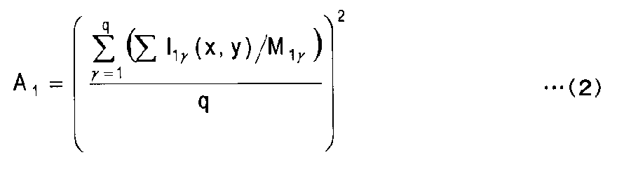
平均値A1は、たとえば次式(2)で表される。
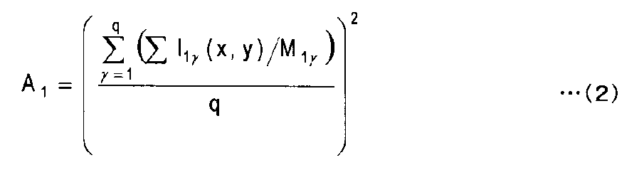
ここで、M1γは、チャンネル1のγフレーム目の計算に使用するデータ数である。
平均値A1の算出式は式(2)に限定されない。平均値A1は、他の周知の任意の計算式を使用して算出されてもよい。
次式(3)は、本実施形態において使用するRICSの解析に使用する空間相互相関計算式を表している。式(3)は、チャンネル1とチャンネル2の相互相関計算式の例である。

ここで、GscはRICSの空間相互相関値、I1γはチャンネル1のγフレーム目の蛍光強度データ(ピクセルのデータ)、I2(γ+η)はチャンネル2の(γ+η)フレーム目の蛍光強度データ(ピクセルのデータ)、x,yは測定点の空間的座標、ξ,ψは測定点からの空間的座標の変化量、γは1以上の整数(γ=1,2,…,q)、ηは0以上q未満の整数(η=0,1,…,p(<q))、M1γ2(γ+η)は、チャンネル1のγフレーム目とチャンネル2の(γ+η)フレーム目の積和計算の回数、A2は平均値である。
γとηは、式(1)の同様に、それぞれ、積和計算の対象の一方のフレームと、γに対するフレーム数の遅れを示している。
平均値A2は、たとえば次式(4)で表される。
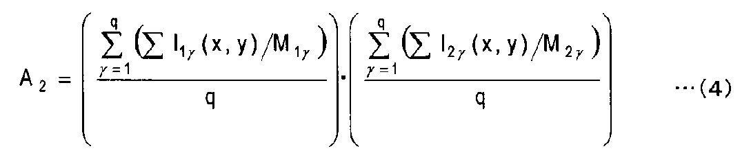
ここで、M1γは、チャンネル1のγフレーム目の計算に使用するデータ数、M2γは、チャンネル2のγフレーム目の計算に使用するデータ数である。
次式(5)は、本実施形態において使用するRICSの解析に使用するフィッティング式を表している。

ここで、GsはRICSの空間相関値(空間自己相関値Gsaまたは空間相互相関値Gsc)、SはRICSの解析におけるスキャンの影響、GはRICSの解析における時間遅延の影響、Dは拡散定数、δrはピクセルサイズ、Nは分子数、W0は励起レーザビームの横方向の半径、WZは励起レーザビームの縦方向の半径、τpはピクセル時間、τlはライン時間、τfはフレーム時間である。
ここで、τpはピクセル間の取得時間のずれである。すなわち、ピクセル時間τpは、1ピクセルのデータを取得するのに要する時間である。またτlは、任意のラインの最初のピクセルと、その次のラインの最初のピクセルとの間の取得時間のずれ(ライン時間)である。すなわち、ライン時間τlは、1ラインを走査するのに要する時間を意味する。またτfは、任意のフレームの最初のピクセルと、その次のフレームの最初のピクセルとの間の取得時間のずれである。すなわち、フレーム時間τfは、1フレームを走査するのに要する時間を意味する。
式(1)~式(4)において、γは、γ=1,2,…,qと表され、ηは、η=0,1,…,pと表され、pとqの間には、p<qの関係がある。q=1の場合(1フレームだけのデータで空間相関計算を行なう場合)、p=0となり、ηの取り得る値は0だけとなる。この場合、本実施形態においてRICSの解析に使用する空間相関計算式とフィッティング式は、η=0の場合には、従来のRICSの解析に使用する空間相関計算式とフィッティング式と同じになる。すなわち、η=0のとき、式(1)の空間自己相関計算式は次式(6)で表される。

ここで、I1はチャンネル1の同一フレームの蛍光強度データ(ピクセルのデータ)、x,yは測定点の空間的座標、ξ,ψは測定点からの空間的座標の変化量、M11はチャンネル1の同一フレーム中の積和計算の回数である。
平均値A1は、次式(7)で表される。

ここで、M1は、チャンネル1の同一フレーム中の計算に使用するデータ数である。
また、式(3)の空間相互相関計算式は次式(8)で表される。

ここで、I1はチャンネル1の計算に使用するフレームの蛍光強度データ(ピクセルのデータ)、I2はチャンネル2の計算に使用するフレームの蛍光強度データ(ピクセルのデータ)、x,yは測定点の空間的座標、ξ,ψは測定点からの空間的座標の変化量、M12はチャンネル1とチャンネル2中のデータの積和計算の回数である。
平均値A2は、次式(9)で表される。

ここで、ここで、M1は、チャンネル1の計算に使用するフレーム中の計算に使用するデータ数、M2は、チャンネル2の計算に使用するフレーム中の計算に使用するデータ数である。
また、式(5)のフィッティング式は次式(10)で表される。
[測定手順]
以下、図3を参照しながら画像解析の手順について説明する。また、各ステップについて、適宜、図4~図12を参照しながら説明する。
以下、図3を参照しながら画像解析の手順について説明する。また、各ステップについて、適宜、図4~図12を参照しながら説明する。
(ステップS1)
試料Sの観察領域と取得する蛍光画像のフレーム数を設定する。設定した観察領域の設定したフレーム数の蛍光画像を時系列的に取得する。蛍光画像の取得は、同一の観察領域に対して同一の走査方法によって行なう。すなわち、所定の方向に向けて光を照射した後、再び当該所定の方向に向けて光を照射するまでを1セットの走査とした場合、少なくとも2セット以上、解析領域が走査される。
試料Sの観察領域と取得する蛍光画像のフレーム数を設定する。設定した観察領域の設定したフレーム数の蛍光画像を時系列的に取得する。蛍光画像の取得は、同一の観察領域に対して同一の走査方法によって行なう。すなわち、所定の方向に向けて光を照射した後、再び当該所定の方向に向けて光を照射するまでを1セットの走査とした場合、少なくとも2セット以上、解析領域が走査される。
画像解析に使用する複数フレームの蛍光画像を模式的に図4に示す。画像解析に使用する複数フレームの蛍光画像は、ステップS1で取得した画像の全部であってもよく、また一部であってもよい。以下では、画像解析に使用する複数フレームの蛍光画像を単に複数フレームの蛍光画像と呼ぶ。図4において、Fkは、一つのチャンネルにおけるkフレーム目の蛍光画像を表している。各蛍光画像は、ピクセルのデータが時系列的に取得された複数のピクセルからなる。ピクセルのデータは、たとえば、2次元または3次元の観察領域から得られた蛍光強度である。
(ステップS2)
図5に示すように、画像解析に使用する蛍光画像の領域(観察領域)R1に対して解析する領域(解析領域)R2を設定する。解析領域R2は、観察領域R1の一部に限定されるものではなく、観察領域R1に一致していてもよい。解析領域R2は、アプリケーション的にはデフォルトで観察領域R1すなわちステップS1における走査領域に設定されている。観察領域R1の全体を解析する場合には、このステップは不要である。
図5に示すように、画像解析に使用する蛍光画像の領域(観察領域)R1に対して解析する領域(解析領域)R2を設定する。解析領域R2は、観察領域R1の一部に限定されるものではなく、観察領域R1に一致していてもよい。解析領域R2は、アプリケーション的にはデフォルトで観察領域R1すなわちステップS1における走査領域に設定されている。観察領域R1の全体を解析する場合には、このステップは不要である。
(ステップS3)
複数フレームの蛍光画像をデータ情報変化に基づいて分類する。たとえば、複数フレームの蛍光画像の解析領域R2の区分値をそれぞれ算出し、算出した区分値に基づいて複数フレームの蛍光画像を複数グループに分類する。区分値は、たとえば、解析領域R2のピクセルのデータの統計値であり、解析領域R2のピクセルのデータの最大値、最小値、平均値、相対差、相対比のいずれかである。ピクセルのデータは、たとえば、2次元または3次元の観察領域から得られた蛍光強度である。相対差は、たとえば、最大値と最小値との差である。
複数フレームの蛍光画像をデータ情報変化に基づいて分類する。たとえば、複数フレームの蛍光画像の解析領域R2の区分値をそれぞれ算出し、算出した区分値に基づいて複数フレームの蛍光画像を複数グループに分類する。区分値は、たとえば、解析領域R2のピクセルのデータの統計値であり、解析領域R2のピクセルのデータの最大値、最小値、平均値、相対差、相対比のいずれかである。ピクセルのデータは、たとえば、2次元または3次元の観察領域から得られた蛍光強度である。相対差は、たとえば、最大値と最小値との差である。
複数グループに分類された複数フレームの蛍光画像の解析領域の画像を模式的に図6に示す。図6において、Fakはkフレーム目の蛍光画像の解析領域の画像を表している。Da,Db,Dc,Dd,De,Dfは、蛍光画像の解析領域の区分値を表している。ここでは、一例として、区分値は6種類あるとしている。図6の例では、Fa1,Fa2,Fa79,Fa80が同じグループに分類され、Fa3,Fa74,Fa75が同じグループに分類され、Fa4,Fa71,Fa72,Fa73が同じグループに分類され、Fa5,Fa76,Fa77,Fa78が同じグループに分類され、Fa6,Fa7が同じグループに分類され、Fa8,Fa9,Fa10が同じグループに分類されている。
(ステップS4)
グループごとに解析領域の平均画像を算出する。平均画像は、各グループに含まれる全ての画像の平均値であってもよく、または各グループに含まれる一部の画像の平均値であってもよい。たとえば、平均画像の算出は、各グループに含まれる画像の数を算出し、算出した画像の数に基づいて各グループの平均画像を算出する。
グループごとに解析領域の平均画像を算出する。平均画像は、各グループに含まれる全ての画像の平均値であってもよく、または各グループに含まれる一部の画像の平均値であってもよい。たとえば、平均画像の算出は、各グループに含まれる画像の数を算出し、算出した画像の数に基づいて各グループの平均画像を算出する。
より具体的には、各グループに含まれる全ての画像について、解析領域を構成するピクセルごとに、ピクセルのデータの平均値を算出する。そして、ピクセルごとに算出された各ピクセルのデータの平均値からなる画像を平均画像としてよい。
さらに、グループごとの平均画像のすべてのピクセルの平均値を算出する。
(ステップS5)
グループごとに解析領域の各画像から平均画像を減算する。これにより画像に共通に重畳する不要なデータが除去される。たとえば、大きい分子や不動分子などの影響を取り除かれる。解析領域の各画像から平均画像を減算するには、たとえば、解析領域を構成するピクセルごとに、各画像のピクセルのデータから平均画像のピクセルのデータを減算し、算出された値からなる画像を得ればよい。
グループごとに解析領域の各画像から平均画像を減算する。これにより画像に共通に重畳する不要なデータが除去される。たとえば、大きい分子や不動分子などの影響を取り除かれる。解析領域の各画像から平均画像を減算するには、たとえば、解析領域を構成するピクセルごとに、各画像のピクセルのデータから平均画像のピクセルのデータを減算し、算出された値からなる画像を得ればよい。
さらに、グループごとに解析領域の各画像に平均値を加算する。これにより減算によって低下した輝度値の低下が補われる。ここでは、平均値を加算する例をあげたが、これに代えて、最小値を加算してもよい。
以下、このように平均画像の減算と平均値の加算を経て算出された画像を解析領域の再構築画像と呼ぶことにする。
ここで、kフレーム目の解析領域の再構築画像をFbkとする。また、区分値Da,Db,Dc,Dd,De,Dfに対応する蛍光画像の解析領域の平均画像をそれぞれAa,Ab,Ac,Ad,Ae,Afとする。ここで、Aa,Ab,Ac,Ad,Ae,Afはそれぞれ相応の平均値を加算済みのものとする。このようにした場合、図6の例では、再構築画像は、Fb1=Fa1-Aa,Fb2=Fa2-Aa,Fb3=Fa3-Ab,Fb4=Fa4-Ac,Fb5=Fa5-Ad,Fb6=Fa6-Ae,Fb7=Fa7-Ae,Fb8=Fa8-Af,Fb9=Fa9-Af,Fb10=Fa10-Af,…,Fb71=Fa71-Ac,Fb72=Fa72-Ac,Fb73=Fa73-Ac,Fb74=Fa74-Ab,Fb75=Fa75-Ab,Fb76=Fa76-Ad,Fb77=Fa77-Ad,Fb78=Fa78-Ad,Fb79=Fa79-Aa,Fb80=Fa80-Aaとなる。
画像解析に使用する蛍光画像の解析領域の画像が同種類のものであること、言い換えれば解析領域のデータ情報変化が実質的にないことがあらかじめ分かっている場合には、ステップS3,S4,S5は省略してよい。
(pとqの値について)
式(1)~(4)の空間相関計算を実施するにあたってpとqの値を決定する必要がある。前述したように、pは、空間相関計算における最大の遅延時間を決めるフレーム数を表し、qは、空間相関計算に使用するフレームの総数を表している。pとqの値が大きいほど、計算に使用するデータ数は多くなるので、計算結果の精度つまり信頼度は増加するが、計算に要する時間は長くなる。反対に、pとqの値が小さいほど、計算に使用するデータ数は少なくなるので、計算に要する時間は短くなるが、計算結果の精度つまり信頼度は低下する。このような理由から、pとqの値は、十分な精度の計算結果が得られる範囲において、なるべく小さく設定するとよい。
式(1)~(4)の空間相関計算を実施するにあたってpとqの値を決定する必要がある。前述したように、pは、空間相関計算における最大の遅延時間を決めるフレーム数を表し、qは、空間相関計算に使用するフレームの総数を表している。pとqの値が大きいほど、計算に使用するデータ数は多くなるので、計算結果の精度つまり信頼度は増加するが、計算に要する時間は長くなる。反対に、pとqの値が小さいほど、計算に使用するデータ数は少なくなるので、計算に要する時間は短くなるが、計算結果の精度つまり信頼度は低下する。このような理由から、pとqの値は、十分な精度の計算結果が得られる範囲において、なるべく小さく設定するとよい。
(ステップS6)
pの値を決定するため、まず、拡散時間を推定する。拡散時間の推定は、式(6)~(10)を使用してRICSの解析をすることにより行なう。具体的には、式(6)~式(9)を使用して、異なる遅延時間に対する相関値Gsをそれぞれ求める。そして、遅延時間と相関値Gsとの関係から、式(10)を使用して、拡散定数と分子数を求める。
pの値を決定するため、まず、拡散時間を推定する。拡散時間の推定は、式(6)~(10)を使用してRICSの解析をすることにより行なう。具体的には、式(6)~式(9)を使用して、異なる遅延時間に対する相関値Gsをそれぞれ求める。そして、遅延時間と相関値Gsとの関係から、式(10)を使用して、拡散定数と分子数を求める。
式(10)において、遅延時間がゼロのときは(ξ=0、ψ=0)、Sは1であり、Gsは1/Nで表せる。したがって、分子数を求めることができる。
拡散定数と拡散時間との関係は次式(11)で表される。この式(11)に基づいて、先に求めた拡散定数から拡散時間を求めることができる。

ここで、Dは拡散定数、τは拡散時間、W0は励起レーザビームの横方向の半径を意味する。
なお、解析の対象が拡散時間の短い分子である場合には、式(6)~式(10)を使用して得られる拡散時間は適切な拡散時間を示している。最大の遅延時間が拡散時間の2倍よりも大きい場合、式(10)を用いて十分にフィッティングできるからである。しかし、解析の対象が拡散時間の長い分子である場合には、式(10)を用いてフィッティングしても、そこから得られる拡散時間は、必ずしも、実際の拡散時間と一致しない。この場合、拡散時間は推定値に過ぎない。
(ステップS7)
pの値を決定するため、次に、次式(12)を使用してpを求める。

pの値を決定するため、次に、次式(12)を使用してpを求める。
ここで、τDは推定拡散時間、ξmax,ψmaxは、1フレーム中の空間的座標の変化の最大値、nは2以上の整数(n≧2)である。
一般に、相関値の算出には、最大の遅延時間が、拡散時間の2倍程度あればよいとされている。最大の遅延時間が、拡散時間の2倍よりも短いと、式(5)を用いて適切にフィッティングすることが困難となる。したがって、少なくともn=2とした上で、式(11)を用いて、pを算出すれば、式(5)を用いて適切にフィッティングすることができると考えられる。ただし、解析結果に求められる精度に応じて、nを3以上の整数に設定してもよい。これにより、式(11)を満足するpを用いた式(1)~式(4)を使用したRICSの解析であれば、適切な解析結果が得られると考えられる。
(ステップS8)
パラメータγの最終値qを決定する。qの値は、前述したように、q>pを満足するものでなければならない。qの値は、たとえば、解析領域がm×mの場合、次式(13)を満足するように決める。

パラメータγの最終値qを決定する。qの値は、前述したように、q>pを満足するものでなければならない。qの値は、たとえば、解析領域がm×mの場合、次式(13)を満足するように決める。
(ステップS9)
ステップS5において算出された再構築画像を、ステップS5において決定したqの値に基づいて複数ブロックに分割する。また、複数ブロックを順序づけ、最初のブロックを、続くステップS10における空間相関計算の計算対象に設定する。
ステップS5において算出された再構築画像を、ステップS5において決定したqの値に基づいて複数ブロックに分割する。また、複数ブロックを順序づけ、最初のブロックを、続くステップS10における空間相関計算の計算対象に設定する。
複数ブロックに分割された複数フレームの蛍光画像の解析領域の再構築画像を模式的に図7に示す。図7には、一例として、80フレームの蛍光画像の解析領域の再構築画像Fb1~Fb80が、8フレームずつ、10個のブロックB1~B10に分割された例が示されている。
(ステップS10)
計算対象のブロックに対して空間相関値を計算する。空間自己相関値を計算する場合は式(1)と式(2)の空間自己相関計算式を使用し、空間相互相関値を計算する場合は式(3)と式(4)の空間相互相関計算式を使用する。
計算対象のブロックに対して空間相関値を計算する。空間自己相関値を計算する場合は式(1)と式(2)の空間自己相関計算式を使用し、空間相互相関値を計算する場合は式(3)と式(4)の空間相互相関計算式を使用する。
相関値の計算に使用する各ピクセルのデータは、そのピクセルのデータそのものであってもよいし、そのピクセルを含む複数のピクセルのデータの統計値であってもよい。複数のピクセルは、たとえば、注目のピクセルおよびこれに隣接するピクセルであってよい。統計値は、たとえば、ピクセルのデータの平均値、最大値、最小値、相対差、絶対差、相対比のいずれかであってよい。どのような統計値を使用するかは、RICSの解析によってどのような情報を得たいかによって決める。
また相関値の計算は、ピクセルのデータに基づいて画像をそれぞれ構成し直し、構成し直した画像について相関値を計算してもよい。たとえば、隣のピクセルのデータ同士を足して、ピクセルのデータの数を半分にする。または、一つのピクセルのデータを複数に分割する。本来ならば、一度画像を取得するとピクセルのデータの数は増えないが、取得したピクセルのデータの強度がそのピクセルのデータの周囲にガウシアン分布で広がっていると仮定して、本来取得できていないピクセルのデータを補う。本質的にピクセルのデータの数が増えている訳ではないが、見た目が良くなる。
式(1)~式(4)を使用する計算は、ηの値を0,1,2,…,pと順に変えつつ、ηの各値に対して、さらにγの値を1,2,…,p-ηと順に変えつつ、さらにγの各値に対して、ξ,ψを順に変えつつ行なう。たとえば、解析領域R2が256ピクセル×256ピクセルの領域である場合、ξ,ψをそれぞれ0,1,2,…,255と順に変える。
たとえば、η=0,γ=1,ψ=0に対して、ξを0,1,2,…,255と1ずつ増やしながら、ξの各値について計算処理を行ない、次にψを1増やし、η=0,γ=1,ψ=1に対して、ξを0,1,2,…,255と1ずつ増やしながら、ξの各値について計算処理を行ない、この計算処理をψ=255になるまで繰り返す。その後、γを1増やし、η=0,γ=2,ψ=0に対して、ξを0,1,2,…,255と1ずつ増やしながら、ξの各値について計算処理を行ない、次に、η=0,γ=2,ψ=1に対して、ξを0,1,2,…,255と1ずつ増やしながら、ξの各値について計算処理を行ない、この計算処理をψ=255になるまで繰り返す。この計算処理をψ=255になるまで繰り返す。この計算処理はγを1ずつ増やしながら、γ=qになるまで繰り返す。
その後、ηを1増やし、η=1,γ=1,ψ=0に対して、ξを0,1,2,…,255と1ずつ増やしながら、ξの各値について計算処理を行ない、次にψを1増やし、η=1,γ=1,ψ=1に対して、ξを0,1,2,…,255と1ずつ増やしながら、ξの各値について計算処理を行ない、この計算処理をψ=255になるまで繰り返す。その後、γを1増やし、η=1,γ=2,ψ=0に対して、ξを0,1,2,…,255と1ずつ増やしながら、ξの各値について計算処理を行ない、次に、η=1,γ=2,ψ=1に対して、ξを0,1,2,…,255と1ずつ増やしながら、ξの各値について計算処理を行ない、この計算処理をψ=255になるまで繰り返す。この計算処理をψ=255になるまで繰り返す。この計算処理はγを1ずつ増やしながら、γ=q-1になるまで繰り返す。
以降、ηを1ずつ増やしながらηの各値に対して、γを1ずつ増やしながら、同様の計算処理を、γ=q-ηになるまで繰り返す。この計算処理は、ηを1ずつ増やしながら、η=pになるまで繰り返す。
図8は、Gs(2,4,0)中の積和計算を模式的に示している。この計算は、同一フレーム(γフレーム目)の再構築画像の解析領域R2内のピクセルのデータ間の相関計算である。この計算において、γの取り得る最終値はqである。
図9は、Gs(2,4,1)中の積和計算を模式的に示している。この計算は、異なるフレームの画像の解析領域R2内のピクセルのデータの間の相関計算である。具体的には、γフレーム目の再構築画像の解析領域R2内のピクセルのデータと(γ+1)フレーム目の再構築画像の解析領域R2内のピクセルのデータとの間の相関計算である。この計算において、γの取り得る最終値はqー1である。
図10は、Gs(2,4,2)中の積和計算を模式的に示している。つまり、γフレーム目の再構築画像の解析領域R2内のピクセルのデータと(γ+2)フレーム目の再構築画像の解析領域R2内のピクセルのデータとの間の相関計算を示している。この計算において、γの取り得る最終値はqー2である。
図11は、Gs(2,4,p)中の積和計算を模式的に示している。つまり、γフレーム目の再構築画像の解析領域R2内のピクセルのデータとpフレーム目の再構築画像の解析領域R2内のピクセルのデータとの間の相関計算を示している。この計算において、γの取り得る最終値はqーpである。
図12は、式(1)~式(4)における変数ξ,ψ,ηと計算に使用するフレームを示している。図12から、本実施形態による式(1)~式(4)を使用した計算では、遅延時間が拡張されていることがわかる。具体的には、遅延時間は、256τp+255τlを超えて、256τp+255τl+pτfまで拡大されている。
ここで、遅延時間とは、一つのピクセルの取得時間と別のピクセルの取得時間との差を意味している。たとえば、(ξ,ψ,η)=(1,1,0)と、(ξ,ψ,η)=(4,2,0)との遅延時間は、(4-1)τp+(2-1)τl+(0-0)τfで表される。
そして、一つの遅延時間に対して、一つの相関値Gsが得られる。ここで、理想的には、遅延時間が小さいほど、相関値Gsは大きくなり、遅延時間が大きいほど、相関値Gsは小さくなる。
(ステップS11)
計算対象のブロックが最終ブロックであるかを判断する。計算対象のブロックが最終ブロックでない場合には、計算対象のブロックを次のブロックに変更してステップS10に戻る。また計算対象のブロックが最終ブロックであい場合には、次のステップS12に進む。
計算対象のブロックが最終ブロックであるかを判断する。計算対象のブロックが最終ブロックでない場合には、計算対象のブロックを次のブロックに変更してステップS10に戻る。また計算対象のブロックが最終ブロックであい場合には、次のステップS12に進む。
(ステップS12)
ステップS11において計算された複数の空間相関値の平均値を計算する。
ステップS11において計算された複数の空間相関値の平均値を計算する。
(ステップS13)
ステップS12において計算された空間相関値を式(5)によってフィッティングする。
ステップS12において計算された空間相関値を式(5)によってフィッティングする。
式(5)によってフィッティングすることにより拡散時間の推定をする。具体的には、式(1)~式(4)を使用して、異なる遅延時間に対する自己相関値Gsaまたは相互相関値Gscをそれぞれ求める。そして、自己相関値Gsaまたは相互相関値Gscと遅延時間との関係から、式(5)を使用して、拡散定数と分子数を求める。
式(5)において、遅延時間がゼロのときは(ξ=0,ψ=0,η=0)、Sは1であり、自己相関値Gsaまたは相互相関値Gscは1/Nで表せる。したがって、分子数を求めることができる。
未知数である拡散定数Dと分子数Nを変動させながら、測定値として得られる相関値Gsaまたは相関値Gscと理論値として得られるGsとの差が最小となるように、適切な拡散定数Dと分子数Nを求める。このように、式(5)によるフィッティングとは、拡散定数Dと分子数Nを変動させながら、2次元または3次元の観察領域における、最適な、分子数または拡散定数を推定することである。
拡散定数と拡散時間との関係を示す式(11)に基づいて、求めた拡散定数から拡散時間を求めることができる。
(ステップS14)
計算結果を表示し保存する。具体的には、ステップS12で得た空間相関平均値と、ステップS14で得た空間相関値のフィッティング結果を表示する。解析結果の一例を図13~図16に示す。図13は、小さい分子に対する空間相関値の計算結果を輝度で示した画像であり、図14は、そのフィッティング結果を示している。また図15は、大きい分子に対する空間相関値の計算結果を輝度で示した画像であり、図16は、そのフィッティング結果を示している。
計算結果を表示し保存する。具体的には、ステップS12で得た空間相関平均値と、ステップS14で得た空間相関値のフィッティング結果を表示する。解析結果の一例を図13~図16に示す。図13は、小さい分子に対する空間相関値の計算結果を輝度で示した画像であり、図14は、そのフィッティング結果を示している。また図15は、大きい分子に対する空間相関値の計算結果を輝度で示した画像であり、図16は、そのフィッティング結果を示している。
RICSのような画像データを計算の元とする空間的相関解析において、本実施形態では、ステップS3~S5において、複数フレームの画像をフレームデータの変化に応じていくつかのグループに分類し、グループごとに平均画像の減算処理を行なっている。つまり、異なる大きい分子や不動分子の影響が混在するフレームから一つの平均画像を算出して減算処理することを避け、大きい分子や不動分子の影響を事前に分類し、分類したグループごとに平均画像を算出して減算処理している。これにより、フレームデータの変化に応じたグループごとに、大きい分子や不動分子の影響が適材適所に除去される。
従来、RICSのような画像データを計算の元とする空間的相関解析では、1フレームの画像の解析領域中のピクセルのデータを用いて一つの相関値を計算する。しかし、細胞観察のような細胞の核、膜、質などの異なる局所的な解析領域に限定してRICSの解析を行なう場合、解析領域が小さくなる。解析領域が小さくなると、積和計算に利用できるピクセルデータの数(たとえば8×8)が減少する。このため、解析領域が非常に小さくなると、相関値が適切に算出できなくなる。図17は、EGFP溶液(色素液を蒸留水で希釈したもの)の拡散定数(D)を解析領域のROIサイズを変えながら比較した結果を示している。図17において、ROIサイズ=256は、解析領域内に256×256のピクセル数が含まれていることを意味する。図17から分かるように、解析領域のROIサイズが大きいほど、EGFP溶液の拡散定数90(理論値)に近い値を示し、解析領域のROIサイズが小さいほど、EGFP溶液の拡散定数90(理論値)から遠い値を示している。すなわち、ピクセルのデータが多いほど、正しい結果(理論値)に近い値(測定値)が得られることが分かる。
これに対して本実施形態では、ステップS10における空間相関値計算において、1フレームの画像の解析領域内の二つのピクセルに対する積和計算によって一つの相関値を計算するのではなく、複数フレーム(qフレーム)の画像の解析領域内の二つのピクセルに対して積和計算を継続的に行なって一つの相関値を計算する。このように複数フレームの画像のデータを使用して一つの相関値を計算するので、相関値の計算に使用するデータが1フレームの画像中のデータに制限されず、一つの相関値の計算に使用するデータの数が増大する。このため、高い精度でRICSの解析を行なえる。
さらに本実施形態では、ステップS10における空間相関値計算において使用する式(1)~(4)は、パラメータηによって遅延時間の拡張が図られている。これにより、ピクセル時間とライン時間を調整することなく、観察可能な拡散時間を拡張できる。このため、データ収集をし直さなくても、すでに取得したデータを用いて試料に適した拡散時間を推測することができる。これにより、大きい拡散時間の分子についても、小さい拡散時間の分子についても、適切な拡散時間を算出することが可能となる。
これまで、図面を参照しながら本発明の実施形態を述べたが、本発明は、これらの実施形態に限定されるものではなく、その要旨を逸脱しない範囲において様々な変形や変更が施されてもよい。
また実施形態では、ラスター走査によって取得された画像について説明したが、画像は、ラスター走査によって取得されたものに限定されるものではなく、ピクセルのデータが時系列的に取得された複数のピクセルからなる画像であればよく、他の走査方法によって取得されたものであってもよい。
100…画像解析装置、110…光照射部、112a,…,112n…光源、114a,…,114n…コリメートレンズ、116a,…,116n…ダイクロイックミラー、122…ダイクロイックミラー、124…ガルバノミラー、126…対物レンズ、128…対物レンズ駆動機構、130…光検出部、132…収束レンズ、134…ピンホール、136…コリメートレンズ、138a,…,138n…ダイクロイックミラー、140a,…,140n…蛍光フィルター、142a,…,142n…光検出器、160…制御部、162…走査制御部、164…画像形成部、166…記憶部、168…表示部、170…入力部、172…解析領域設定部、174…画像選定部、176…データ抽出部、178…解析部、180…ステージ制御部、190…試料ステージ、R1…観察領域、R2…解析領域。
Claims (24)
- 各画像のピクセルのデータが時系列的に取得された複数のピクセルからなる複数フレームの画像を時系列的に取得する画像取得ステップと、
前記複数フレームの各画像に対して解析領域を設定する解析領域設定ステップと、
前記複数フレームの画像の中から解析に利用する2フレーム以上の選定画像を選定する画像選定ステップと、
前記選定画像の同一画像の前記解析領域内の取得時間間隔が同じ二つのピクセルのデータペアの積和計算を前記選定画像のすべてに対して行なうとともに、前記選定画像の異なる二つの画像の前記解析領域内の取得時間間隔が同じ二つのピクセルのデータペアの積和計算を行なって相関値を計算する演算ステップとを有している画像解析方法。 - 前記解析領域の区分値を算出する区分値算出ステップと、
前記複数フレームの画像を前記区分値に基づいて複数グループに分類する分類ステップと、
前記グループごとに前記解析領域の平均画像を算出する平均画像算出ステップと、
前記グループごとに前記解析領域の各画像から前記平均画像を減算して前記解析領域の再構築画像を算出する再構築画像算出ステップとをさらに有し、
前記演算ステップは、再構築画像に対して相関値を計算する、請求項1に記載の画像解析方法。 - 前記複数フレームの画像を複数ブロックに分割するステップをさらに有し、
前記演算ステップは、前記複数ブロックごとに相関値を計算し、
前記複数ブロックごとに計算された相関値の平均値を計算するステップをさらに有している、請求項1または2に記載の画像解析方法。 - 前記データペアの各々は、前記ピクセルのデータの統計値であり、前記統計値は、前記ピクセルのデータの平均値、最大値、最小値、相対差、絶対差、相対比のいずれかである、請求項1ないし請求項3のいずれかひとつに記載の画像解析方法。
- 前記ピクセルのデータは、2次元または3次元の観察領域から得られた蛍光強度である、請求項1ないし請求項4のいずれかひとつに記載の画像解析方法。
- 前記演算ステップは、前記ピクセルのデータに基づいて、前記複数の画像をそれぞれ構成し直し、構成し直した画像について相関値を演算する、請求項1ないし5のいずれかひとつに記載の画像解析方法。
- 前記画像は、走査型顕微鏡によって得られたものである、請求項1ないし6のいずれかひとつに記載の画像解析方法。
- 前記演算ステップは、次式(1)を用いて、2次元または3次元の観察領域の自己相関の計算を行なう、

- 前記平均値A1は次式(2)で表される、
- 前記演算ステップは、次式(3)を用いて、2次元または3次元の観察領域の相互相関値の計算を行なう、

- 平均値A2は、たとえば次式(4)で表される、
- 前記演算ステップは、次式(5)を用いて、前記空間相関値の計算結果をフィッティングし、分子数または拡散定数を推定する、

- 各画像のピクセルのデータが時系列的に取得された複数のピクセルからなる複数フレームの画像を時系列的に取得する画像取得部と、
前記複数フレームの各画像に対して解析領域を設定する解析領域設定部と、
前記複数フレームの画像の中から解析に利用する2フレーム以上の選定画像を選定する画像選定部と、
前記選定画像の同一画像の前記解析領域内の取得時間間隔が同じ二つのピクセルのデータペアの積和計算を前記選定画像のすべてに対して行なうとともに、前記選定画像の異なる二つの画像の前記解析領域内の取得時間間隔が同じ二つのピクセルのデータペアの積和計算を行なって相関値を計算する演算部とを有している画像解析装置。 - 前記演算部は、
前記解析領域の区分値を算出し、
前記複数フレームの画像を前記区分値に基づいて複数グループに分類し、
前記グループごとに前記解析領域の平均画像を算出し、
前記グループごとに前記解析領域の各画像から前記平均画像を減算して前記解析領域の再構築画像を算出し、
再構築画像に対して相関値を計算する、請求項13に記載の画像解析装置。 - 前記演算部は、
前記複数フレームの画像を複数ブロックに分割し、
前記複数ブロックごとに相関値を計算し、
前記複数ブロックごとに計算された相関値の平均値を計算する、請求項13または14に記載の画像解析装置。 - 前記データペアの各々は、前記ピクセルのデータの統計値であり、前記統計値は、前記ピクセルのデータの平均値、最大値、最小値、相対差、絶対差、相対比のいずれかである、請求項13ないし15のいずれかひとつに記載の画像解析装置。
- 前記ピクセルのデータは、2次元または3次元の観察領域から得られた蛍光強度である、請求項13ないし16のいずれかひとつに記載の画像解析装置。
- 前記演算部は、前記ピクセルのデータに基づいて、前記複数の画像をそれぞれ構成し直し、構成し直した画像について相関値を演算する、請求項13ないし17のいずれかひとつに記載の画像解析装置。
- 前記画像は、走査型顕微鏡によって得られたものである、請求項13ないし18のいずれかひとつに記載の画像解析装置。
- 前記演算部は、次式(1)を用いて、2次元または3次元の観察領域の自己相関の計算を行なう、

- 前記平均値A1は次式(2)で表される、
- 前記演算部は、次式(3)を用いて、2次元または3次元の観察領域の相互相関値の計算を行なう、

- 平均値A2は、たとえば次式(4)で表される、

- 前記演算部は、次式(5)を用いて、前記空間相関値の計算結果をフィッティングし、分子数または拡散定数を推定する、

Applications Claiming Priority (2)
| Application Number | Priority Date | Filing Date | Title |
|---|---|---|---|
| JP2009238442A JP5508809B2 (ja) | 2009-10-15 | 2009-10-15 | 画像解析方法および画像解析装置 |
| JP2009-238442 | 2009-10-15 |
Publications (2)
| Publication Number | Publication Date |
|---|---|
| WO2011046212A1 true WO2011046212A1 (ja) | 2011-04-21 |
| WO2011046212A9 WO2011046212A9 (ja) | 2011-07-07 |
Family
ID=43876261
Family Applications (1)
| Application Number | Title | Priority Date | Filing Date |
|---|---|---|---|
| PCT/JP2010/068192 Ceased WO2011046212A1 (ja) | 2009-10-15 | 2010-10-15 | 画像解析方法および画像解析装置 |
Country Status (2)
| Country | Link |
|---|---|
| JP (1) | JP5508809B2 (ja) |
| WO (1) | WO2011046212A1 (ja) |
Cited By (2)
| Publication number | Priority date | Publication date | Assignee | Title |
|---|---|---|---|---|
| WO2013069393A1 (ja) * | 2011-11-10 | 2013-05-16 | オリンパス株式会社 | 画像解析方法および画像解析装置 |
| EP2623957A4 (en) * | 2010-10-29 | 2016-01-27 | Olympus Corp | IMAGE ANALYSIS METHOD AND IMAGE ANALYSIS DEVICE |
Families Citing this family (1)
| Publication number | Priority date | Publication date | Assignee | Title |
|---|---|---|---|---|
| JP2012008055A (ja) * | 2010-06-25 | 2012-01-12 | Olympus Corp | 画像解析方法および画像解析装置 |
Citations (5)
| Publication number | Priority date | Publication date | Assignee | Title |
|---|---|---|---|---|
| JP2004108892A (ja) * | 2002-09-17 | 2004-04-08 | Olympus Corp | 蛍光分光分析装置 |
| JP2006078377A (ja) * | 2004-09-10 | 2006-03-23 | Olympus Corp | 光信号解析方法 |
| JP2008276191A (ja) * | 2007-05-02 | 2008-11-13 | Olympus Corp | 蛍光顕微鏡装置 |
| JP2010217716A (ja) * | 2009-03-18 | 2010-09-30 | Victor Co Of Japan Ltd | 電子機器 |
| JP2010237116A (ja) * | 2009-03-31 | 2010-10-21 | Olympus Corp | 画像解析方法および画像解析装置 |
Family Cites Families (5)
| Publication number | Priority date | Publication date | Assignee | Title |
|---|---|---|---|---|
| JPH0993588A (ja) * | 1995-09-28 | 1997-04-04 | Toshiba Corp | 動画像処理方法 |
| JP5161427B2 (ja) * | 2006-02-20 | 2013-03-13 | 株式会社東芝 | 画像撮影装置、画像処理装置及びプログラム |
| WO2008087869A1 (ja) * | 2007-01-16 | 2008-07-24 | Olympus Corporation | 蛍光信号解析装置および蛍光信号解析方法 |
| JP5208824B2 (ja) * | 2009-03-18 | 2013-06-12 | オリンパス株式会社 | 画像取得装置、画像取得方法及びプログラム |
| JP5566055B2 (ja) * | 2009-07-10 | 2014-08-06 | オリンパス株式会社 | 画像解析方法および画像解析装置 |
-
2009
- 2009-10-15 JP JP2009238442A patent/JP5508809B2/ja active Active
-
2010
- 2010-10-15 WO PCT/JP2010/068192 patent/WO2011046212A1/ja not_active Ceased
Patent Citations (5)
| Publication number | Priority date | Publication date | Assignee | Title |
|---|---|---|---|---|
| JP2004108892A (ja) * | 2002-09-17 | 2004-04-08 | Olympus Corp | 蛍光分光分析装置 |
| JP2006078377A (ja) * | 2004-09-10 | 2006-03-23 | Olympus Corp | 光信号解析方法 |
| JP2008276191A (ja) * | 2007-05-02 | 2008-11-13 | Olympus Corp | 蛍光顕微鏡装置 |
| JP2010217716A (ja) * | 2009-03-18 | 2010-09-30 | Victor Co Of Japan Ltd | 電子機器 |
| JP2010237116A (ja) * | 2009-03-31 | 2010-10-21 | Olympus Corp | 画像解析方法および画像解析装置 |
Non-Patent Citations (1)
| Title |
|---|
| MICHELLE A. DIGMAN ET AL.: "Measuring Fast Dynamics in Solutions and Cells with a Laser Scanning Microscope", BIOPHYSICAL JOURNAL, vol. 89, August 2005 (2005-08-01), pages 1317 - 1327, XP002557976 * |
Cited By (5)
| Publication number | Priority date | Publication date | Assignee | Title |
|---|---|---|---|---|
| EP2623957A4 (en) * | 2010-10-29 | 2016-01-27 | Olympus Corp | IMAGE ANALYSIS METHOD AND IMAGE ANALYSIS DEVICE |
| US9330338B2 (en) | 2010-10-29 | 2016-05-03 | Olympus Corporation | Image analysis method and image analysis device |
| WO2013069393A1 (ja) * | 2011-11-10 | 2013-05-16 | オリンパス株式会社 | 画像解析方法および画像解析装置 |
| JP2013104674A (ja) * | 2011-11-10 | 2013-05-30 | Olympus Corp | 画像解析方法および画像解析装置 |
| US9262667B2 (en) | 2011-11-10 | 2016-02-16 | Olympus Corporation | Image analysis method and image analysis apparatus |
Also Published As
| Publication number | Publication date |
|---|---|
| WO2011046212A9 (ja) | 2011-07-07 |
| JP2011085486A (ja) | 2011-04-28 |
| JP5508809B2 (ja) | 2014-06-04 |
Similar Documents
| Publication | Publication Date | Title |
|---|---|---|
| US8908993B2 (en) | Image analysis method and image analysis apparatus | |
| JP5489469B2 (ja) | 蛍光信号解析装置および蛍光信号解析方法 | |
| JP5508808B2 (ja) | 画像解析方法および画像解析装置 | |
| US20220205919A1 (en) | Widefield, high-speed optical sectioning | |
| JP5468805B2 (ja) | 画像解析方法および画像解析装置 | |
| JP2012008055A5 (ja) | ||
| WO2012056580A1 (ja) | 画像解析方法および画像解析装置 | |
| CN105247346A (zh) | 光谱显微镜装置 | |
| JP5566055B2 (ja) | 画像解析方法および画像解析装置 | |
| CN114442298A (zh) | 用于捕获图像数据的设备和方法 | |
| WO2013080808A1 (ja) | 画像処理装置、顕微鏡システム、画像処理方法、及び画像処理プログラム | |
| JP5856814B2 (ja) | 画像解析方法および画像解析装置 | |
| JP5508809B2 (ja) | 画像解析方法および画像解析装置 | |
| CN103180718B (zh) | 图像分析方法以及图像分析装置 | |
| JP5489541B2 (ja) | 画像解析方法および画像解析装置 |
Legal Events
| Date | Code | Title | Description |
|---|---|---|---|
| 121 | Ep: the epo has been informed by wipo that ep was designated in this application |
Ref document number: 10823480 Country of ref document: EP Kind code of ref document: A1 |
|
| NENP | Non-entry into the national phase |
Ref country code: DE |
|
| 122 | Ep: pct application non-entry in european phase |
Ref document number: 10823480 Country of ref document: EP Kind code of ref document: A1 |