WO2011007485A1 - 光学系および撮像装置 - Google Patents
光学系および撮像装置 Download PDFInfo
- Publication number
- WO2011007485A1 WO2011007485A1 PCT/JP2010/002986 JP2010002986W WO2011007485A1 WO 2011007485 A1 WO2011007485 A1 WO 2011007485A1 JP 2010002986 W JP2010002986 W JP 2010002986W WO 2011007485 A1 WO2011007485 A1 WO 2011007485A1
- Authority
- WO
- WIPO (PCT)
- Prior art keywords
- optical system
- optical
- region
- imaging portion
- low
- Prior art date
- Legal status (The legal status is an assumption and is not a legal conclusion. Google has not performed a legal analysis and makes no representation as to the accuracy of the status listed.)
- Ceased
Links
Images










Classifications
-
- G—PHYSICS
- G02—OPTICS
- G02B—OPTICAL ELEMENTS, SYSTEMS OR APPARATUS
- G02B13/00—Optical objectives specially designed for the purposes specified below
- G02B13/18—Optical objectives specially designed for the purposes specified below with lenses having one or more non-spherical faces, e.g. for reducing geometrical aberration
-
- G—PHYSICS
- G02—OPTICS
- G02B—OPTICAL ELEMENTS, SYSTEMS OR APPARATUS
- G02B13/00—Optical objectives specially designed for the purposes specified below
- G02B13/24—Optical objectives specially designed for the purposes specified below for reproducing or copying at short object distances
-
- G—PHYSICS
- G02—OPTICS
- G02B—OPTICAL ELEMENTS, SYSTEMS OR APPARATUS
- G02B9/00—Optical objectives characterised both by the number of the components and their arrangements according to their sign, i.e. + or -
- G02B9/34—Optical objectives characterised both by the number of the components and their arrangements according to their sign, i.e. + or - having four components only
- G02B9/36—Optical objectives characterised both by the number of the components and their arrangements according to their sign, i.e. + or - having four components only arranged + -- +
- G02B9/38—Optical objectives characterised both by the number of the components and their arrangements according to their sign, i.e. + or - having four components only arranged + -- + both - components being meniscus
- G02B9/42—Optical objectives characterised both by the number of the components and their arrangements according to their sign, i.e. + or - having four components only arranged + -- + both - components being meniscus two - components being compound
Definitions
- the present invention relates to an optical system and an imaging apparatus.
- a dual-focus optical system is known in which it can be considered that the focal point is located at two points before and after the original focal point in the optical axis direction (see, for example, Patent Document 1).
- a bifocal lens system is known in which object points with different object point distances can be simultaneously imaged without moving parts (see, for example, Patent Document 2).
- a technique is known in which the optical transfer function of the optical system is kept substantially constant within a certain range from the focal position by using a phase mask (see, for example, Patent Document 3).
- a technique is known in which an optical transfer function of optical imaging is substantially unchanged with respect to a focal aberration by an optical element that changes the phase of the wavefront (see, for example, Patent Document 4).
- Patent Document 1 Japanese Patent Application Laid-Open No. 7-84221 Patent Document 2 Japanese Patent Application Laid-Open Publication No. 2003-270526 Patent Document 3 Japanese Patent Publication No. 11-500235 Japanese Patent Application Laid-Open No. 2006-523330
- an optical system is a low image formation having an optical parameter that provides an image formation characteristic lower than an image formation characteristic provided by an optical parameter of another region.
- the optical transfer function of the optical system with respect to light from an object point passing through the low imaging portion and other regions is substantially the same regardless of the distance to the object point.
- the optical system may spread the light from the object point passing through the low imaging portion and other regions to substantially the same size regardless of the distance to the object point.
- the low imaging portion may be a region including the optical axis, and the other region may be a region not including the optical axis around the low imaging portion.
- the low imaging portion is formed in a partial region including the optical axis of at least one surface of at least one lens of the optical system, and has imaging characteristics given by the optical parameters of the region not including the optical axis of the surface. It may have optical parameters that give low imaging properties.
- the low imaging portion may have a curved surface shape that provides imaging characteristics lower than the imaging properties provided by the curved surface shape of the region that does not include the optical axis.
- the reference radius of curvature of the low imaging portion may be larger than the reference radius of curvature of other regions.
- the reference radius of curvature of the low imaging portion may be substantially infinite.
- a and b may satisfy 0.08 ⁇ a / b ⁇ 0.60.
- a and b may satisfy 0.11 ⁇ a / b ⁇ 0.43.
- the back focus value fb1 due to the curved surface shape in the low imaging portion, the back focus value fb2 due to the curved surface shape in the other region, and the F number value FN of the optical system are 2.4 ⁇ (fb2 / fb1) ⁇ FN. ⁇ 2.87 may be satisfied.
- the imaging apparatus includes the optical system and a light receiving unit that receives light that has passed through the lens system.
- the light receiving unit has a plurality of light receiving elements respectively corresponding to the plurality of pixels, the plurality of pixels each receive light transmitted through one color of at least three color filters, and the optical system receives three colors of light.
- the size may be larger than a pixel block formed by three adjacent pixels that receive light.
- FIG. 2 is a diagram illustrating a lens configuration of a lens system 110.
- FIG. It is a figure which shows the image height and defocus dependence of the spot diagram in Numerical Example 1.
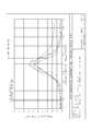
- FIG. It is a figure which shows the depth versus MTF in Numerical Example 1.
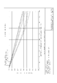
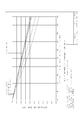
- FIG. It is a figure which shows the spatial frequency versus MTF in Numerical Example 1 with a diffraction limit.
- FIG. 6 is a diagram showing another lens configuration of the lens system 110.
- FIG. 6 is a diagram showing still another lens configuration of the lens system 110. It is a figure which shows the image height and defocus dependence of the spot diagram in Numerical Example 3. It is a figure which shows the depth versus MTF in the numerical Example 3. FIG. It is a figure which shows the spatial frequency versus MTF in Numerical Example 3 with a diffraction limit.
- FIG. 6 is a diagram showing still another lens configuration of the lens system 110.
- FIG. 6 is a diagram showing still another lens configuration of the lens system 110. It is a figure which shows the image height and defocus dependence of the spot diagram in Numerical Example 5. FIG. It is a figure which shows the depth versus MTF in the numerical Example 5. FIG. It is a figure which shows the spatial frequency versus MTF in Numerical Example 5 with a diffraction limit.
- FIG. 6 is a diagram showing still another lens configuration of the lens system 110.
- FIG. 6 is a diagram showing still another lens configuration of the lens system 110. It is a figure which shows the image height and defocus dependence of the spot diagram in Numerical Example 6. It is a figure which shows the depth versus MTF in the numerical Example 6. FIG. It is a figure which shows the spatial frequency versus MTF in the numerical Example 6 with a diffraction limit.
- FIG. 6 is a diagram showing still another lens configuration of the lens system 110.
- FIG. 1 shows an example of a block configuration of an imaging apparatus 100 according to an embodiment.
- the imaging apparatus 100 includes a lens system 110, a light receiving unit 120 that receives light that has passed through the lens system 110, a correction unit 140, an image processing unit 145, and an output unit 150.
- the lens system 110 has substantially the same optical transfer function regardless of the distance to the object point.
- the optical characteristics of the lens system 110 will be qualitatively described with reference to FIG. 2B. Also, an embodiment will be described with reference to FIGS. 3A to 9D.
- the light receiving unit 120 has a plurality of light receiving elements arranged two-dimensionally. Each of the plurality of light receiving elements receives light that has passed through the lens system 110, and outputs a light reception signal having a magnitude corresponding to the amount of light received.
- the correction unit 140 acquires a digital light reception signal obtained by A / D converting the light reception signals output from the plurality of light receiving elements.
- This digital light reception signal can be regarded as a value that is substantially linear with respect to the amount of light received by a plurality of light receiving elements.
- the correction unit 140 performs correction processing on the image represented by the acquired digital light reception signal. For example, the correction unit 140 corrects the image based on the pixel value corresponding to each light receiving element, the position of each light receiving element, and the optical transfer function of the lens system 110. As described above, the correction unit 140 corrects the image obtained by the light received by the light receiving unit 120 based on the optical transfer function of the lens system 110.
- the image processing unit 145 performs image processing on the image corrected by the correction unit 140. Examples of image processing performed by the image processing unit 145 include color balance processing, ⁇ conversion, color synchronization processing, contour correction processing, and color correction processing.
- the output unit 150 outputs an image obtained by processing by the image correction unit 140 and the image processing unit 145.
- the output unit 150 may display the obtained processed image.
- the output unit 150 may record the processed image on a recording medium.
- the output unit 150 may send the processed image to the communication line.
- the output unit 150 may compress the processed image and output the compressed processed image.
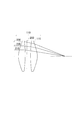
- FIG. 2A schematically shows the imaging characteristics of the ideal lens system.
- the light ray 210, the light ray 220, and the light ray 230 from the object point at infinity on the optical axis are imaged at one point on the optical axis. If the image plane is located at the main imaging point, a single point image can be obtained. However, if the image plane is defocused from the main imaging point, the spread of the point image will increase according to the defocus amount. .
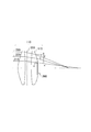
- FIG. 2B qualitatively shows an example of the optical characteristics of the lens system 110 in one embodiment.
- the lens system 110 has a substantially flat low imaging region 260 on the optical surface on the image side of the lens 115 closest to the image plane.
- the low imaging region 260 is a circular cross-sectional region centered on the optical axis.
- the lens system 110 is assumed to have the same optical parameters as the ideal lens system described with reference to FIG. 2A except that the lens system 110 has a low imaging region 260.
- the light ray 220 and the light ray 230 are light rays that do not pass through the low imaging region 260, and are imaged at one point on the optical axis by the lens system 110, similarly to the ideal lens system.
- the light ray 210 is assumed to be a light ray that passes through a position farthest from the optical axis on the low imaging region 260.
- the light ray 210 intersects the optical axis at a position farther from the image formation point of the light rays 220 and 230 due to the presence of the low image formation region 260. Further, other light rays passing through other heights on the low imaging region 260 intersect the optical axis at a position further away from the intersection between the light ray 210 and the optical axis.
- the lens system 110 there is no image plane position where a single point image can be obtained, and a point image having a certain extent can be obtained regardless of the position of the image plane on the optical axis.
- the spread point image can be substantially restored to a single point image.
- the lens system 110 it can be expected that even if the image plane position is defocused, the change in the spread of the point image according to the defocus amount can be significantly reduced as compared with the ideal lens system. If the spread of the point image becomes substantially constant at an image plane position within a predetermined range in the optical axis direction, any point image obtained at the image plane position within the range is transmitted in reverse, for example, corresponding to the predetermined image plane position. By the function restoration process, it can be restored to a point image that is approximately one point. In this case, it can be said that the lens system 110 substantially has a relatively deep depth of focus.
- the relationship between the heights a and b through which the light passes and the heights a ′ and b ′ of the light projected onto the pupil plane 250 is generally proportional.
- the comparison is made at the ratio of a / b.
- a / b a ′ / b ′ is generally obtained, it is possible to make a comparison with a value (a ′ / b ′) converted to the pupil plane. It is.
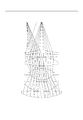
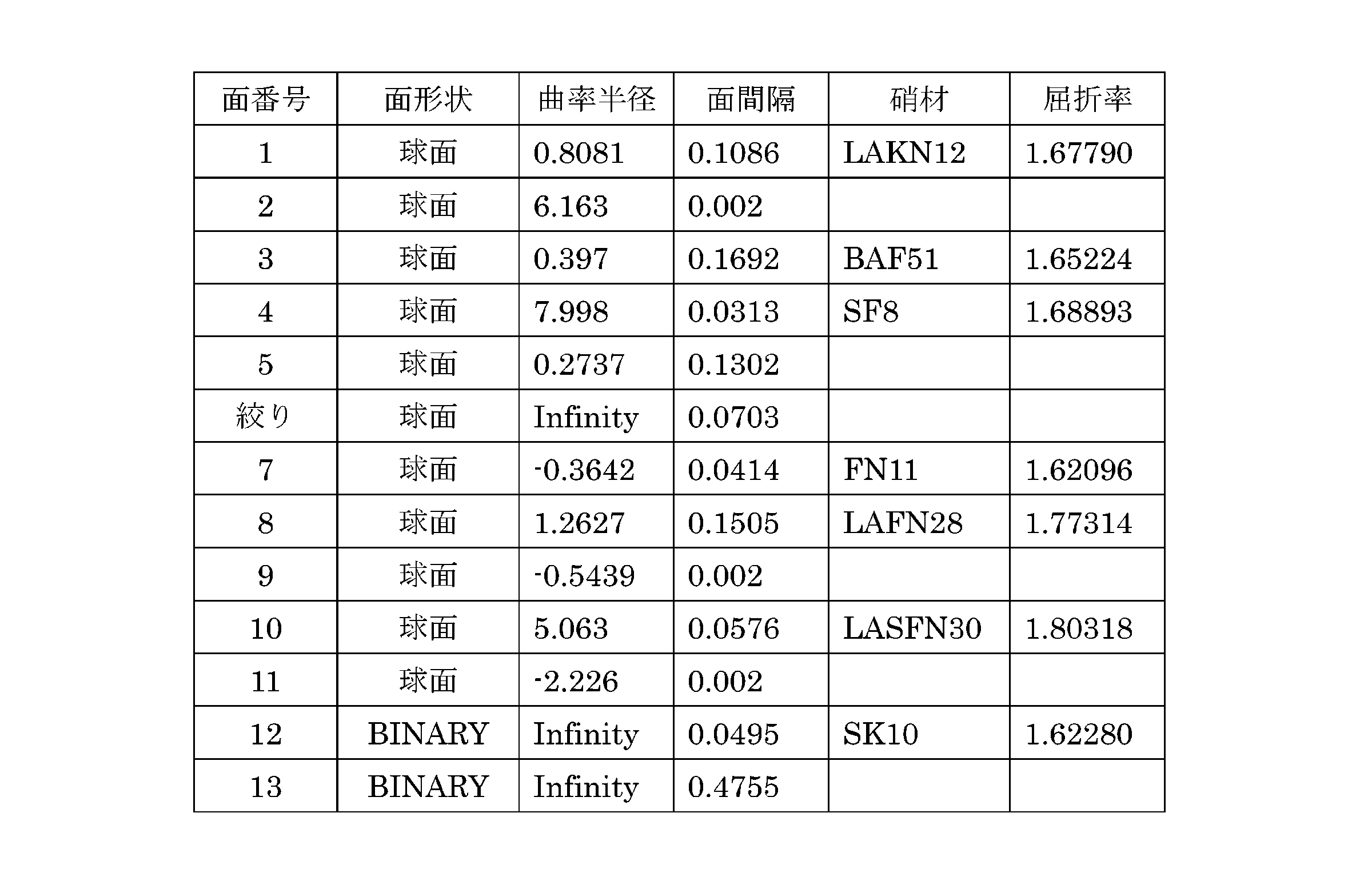
- FIG. 3A shows the lens configuration of the lens system 110.
- Table 1 shows the values of specifications of Numerical Example 1 of the lens system 110 shown in FIG. 3A.
- the surface number, surface shape, radius of curvature, surface interval, glass material, and refractive index indicate the following specifications.
- the surface number i indicates the i-th optical surface counted from the object side.
- the surface number corresponding to the surface representing the aperture is indicated as “aperture”.
- the surface shape indicates “spherical surface” when the optical surface is spherical, “aspherical surface” when the optical surface is aspherical, and the like.
- the radius of curvature indicates the radius of curvature of the i-th optical surface.
- the surface separation indicates the surface separation on the axis between the i-th optical surface and the (i + 1) -th optical surface from the object side.
- the refractive index indicates the refractive index with respect to d-line (587.562 nm) of a glass material having the i-th optical surface on the object side.
- the curvature radius Infinity indicates that the optical surface is a plane (perpendicular to the optical axis).
- the surface shape BINARY indicates that the optical surface is defined by two different surface shape parameters.
- the specifications of surface number 12 and surface number 13 in Numerical Example 1 are shown in Tables 2 and 3, respectively.
- radius of curvature, cone constant, H 4 , H 6 , H 8 , and H 10 indicate the specifications of the optical surface defined by the surface number. That is, the radius of curvature and the conical constant indicate the reference radius of curvature of the optical surface.
- H4, H6, H8, and H10 indicate fourth-order, sixth-order, eighth-order, and tenth-order aspheric expansion coefficients, respectively. That is, Hn represents an nth-order aspheric expansion coefficient. The same applies to other tables.
- the zig z of the optical surface is expressed by the following equation.
- 3B to 3D show spot diagram diagrams and MTF characteristics as the imaging characteristics of Numerical Example 1.
- FIG. Also in other numerical examples described later, imaging characteristics similar to the spot diagram and MTF characteristics described below are shown.
- FIG. 3B shows the image height and defocus dependence of the spot diagram in Numerical Example 1.
- the spot diameter has a relatively constant size with respect to defocus. It should be noted that a predetermined spread is observed at defocus 0. Note that the position of defocus 0 is determined from the balance with the peripheral performance in the vicinity of the position on the optical axis where the value of the center MTF reaches a peak.
- FIG. 3C shows depth versus MTF in Numerical Example 1. Referring to this figure, it can be seen that the maximum value of MTF is relatively low, about 0.57. It can also be seen that the distribution of MTF is relatively wide, and there is a considerable intensity response at the defocused position.
- the depth of focus of the lens system is often evaluated by a width having a predetermined ratio (for example, 20%) of intensity with respect to the maximum MTF value in the distribution of depth versus MTF.
- imaging can be performed with a sensitivity corresponding to the above-described relatively low MTF value, and in the image restoration processing, processing for substantially raising the MTF value is performed. Therefore, also in this lens system 110, the depth of focus can be evaluated at an MTF value having a predetermined value with respect to the maximum MTF value. Since the MTF distribution is relatively wide as shown in the figure, it can be seen that the present numerical example has a relatively long depth of focus. The actual evaluation value of the depth of focus will be described later together with other numerical examples.
- Table 5 and Table 6 show the specifications of the zones of surface number 12 and surface number 13 in Numerical Example 2.
- the specifications in Table 5 and Table 6 are the same as the specifications in Table 2 and Table 3, and thus the description thereof is omitted. Similar specifications are shown for the specifications of each zone in the numerical examples described below.
- FIG. 4B to 4D show spot diagram diagrams and MTF characteristics as imaging characteristics of Numerical Example 2.
- FIG. 4B shows the image height and defocus dependence of the spot diagram in Numerical Example 2. Referring to this figure, it should be noted that a predetermined spread is recognized at defocus 0.
- FIG. 4D shows the spatial frequency versus MTF in Numerical Example 1 together with the diffraction limit. It can be seen that it has a frequency response up to a relatively high frequency region. For this reason, it turns out that the high frequency signal can be restored by the restoration process.
- FIG. 5A shows still another lens configuration of the lens system 110.
- Table 7 shows the values of specifications of Numerical Example 3 of the lens system 110 shown in FIG. 5A.
- Table 8 and Table 9 show the specifications of the zones of surface number 12 and surface number 13 in Numerical Example 3.
- FIG. 5B to 5D show spot diagram diagrams and MTF characteristics as the imaging characteristics of Numerical Example 4.
- FIG. 5B shows the image height and defocus dependence of the spot diagram in Numerical Example 4. Referring to this figure, it should be noted that a predetermined spread of the spot diagram is observed at defocus 0.
- FIG. 5C shows depth versus MTF in Numerical Example 4. Referring to this figure, it can be seen that the maximum value of MTF is relatively low, about 0.46, and the MTF distribution is relatively wide. Therefore, it can be seen that it has a relatively deep depth of focus.
- FIG. 5D shows the spatial frequency versus MTF in Numerical Example 4 together with the diffraction limit. Referring to this figure, it can be seen that the spatial frequency pair MTF is relatively matched regardless of the image height. It can also be seen that the frequency response is relatively high.
- FIG. 6A shows still another lens configuration of the lens system 110.
- Table 10 shows values of specifications of the numerical example 4 of the lens system 110 illustrated in FIG. 6A.
- Table 11 and Table 12 show the specifications of the zones of surface number 12 and surface number 13 in the numerical value example 4.
- FIG. 6B to 6D show spot diagram diagrams and MTF characteristics as the imaging characteristics of Numerical Example 4.
- FIG. 6B shows the image height and defocus dependence of the spot diagram in Numerical Example 4. Referring to this figure, it should be noted that a predetermined spread of the spot diagram is observed at defocus 0.
- FIG. 6C shows depth versus MTF in Numerical Example 4. Referring to this figure, it can be seen that the maximum value of MTF is relatively low, about 0.62, and the MTF distribution is relatively wide. Therefore, it can be seen that it has a relatively deep depth of focus.
- FIG. 6D shows the spatial frequency versus MTF in Numerical Example 5 together with the diffraction limit. Referring to this figure, it can be seen that the spatial frequency pair MTF is relatively matched regardless of the image height. It can also be seen that the frequency response is relatively high.
- FIG. 7A shows still another lens configuration of the lens system 110.
- Table 10 shows values of specifications of Numerical Example 5 of the lens system 110 illustrated in FIG. 7A.
- Table 14 and Table 15 show the specifications of the zones of the surface number 12 and the surface number 13 in this numerical example 5.
- FIG. 7B to 7D show spot diagram diagrams and MTF characteristics as imaging characteristics of Numerical Example 5.
- FIG. 7B shows the image height and defocus dependence of the spot diagram in Numerical Example 5. Referring to this figure, it should be noted that a predetermined spread of the spot diagram is observed at defocus 0.
- FIG. 7C shows depth versus MTF in Numerical Example 5. Referring to this figure, it can be seen that the maximum value of MTF is relatively low, about 0.65, and the MTF distribution is relatively wide. Therefore, it can be seen that it has a relatively deep depth of focus.
- FIG. 7D shows the spatial frequency versus MTF in Numerical Example 5 together with the diffraction limit. Referring to this figure, it can be seen that the spatial frequency pair MTF is relatively matched regardless of the image height. It can also be seen that the frequency response is relatively high.
- FIG. 8A shows still another lens configuration of the lens system 110.
- Table 16 shows values of specifications of Numerical Example 6 of the lens system 110 illustrated in FIG. 8A.
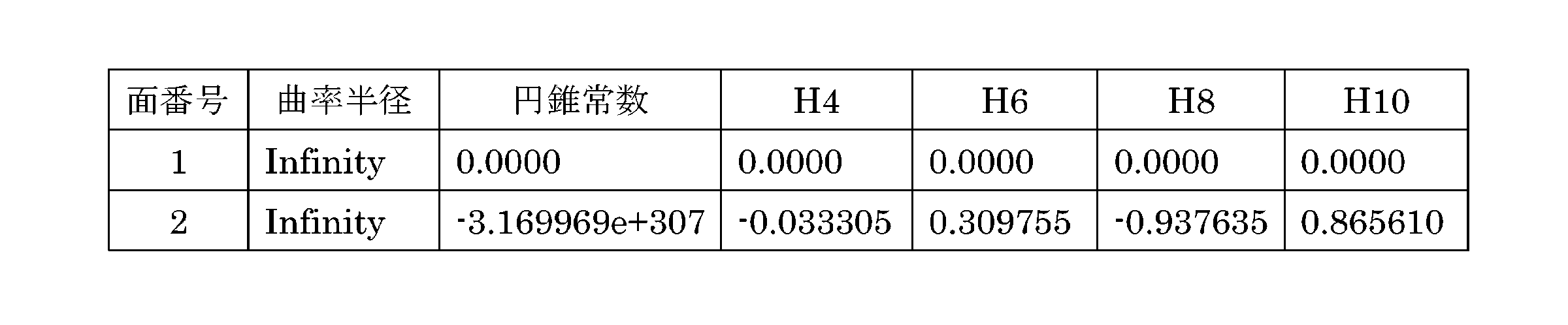
- Table 17 and Table 18 show the specifications of each zone of surface number 1 and surface number 2 in this numerical example 6.
- the aspheric surface data of surface number 5-12 of the aspheric surface in Numerical Example 6 are shown in Table 19A to Table 19D.
- a reference radius of curvature which is one parameter that defines the surface shape of the aspheric surface, is described.
- FIG. 8B to 8D show spot diagram diagrams and MTF characteristics as imaging characteristics of Numerical Example 6.
- FIG. 8B shows the image height and defocus dependence of the spot diagram in Numerical Example 6. Referring to this figure, it should be noted that a predetermined spread of the spot diagram is observed at defocus 0.
- FIG. 8C shows depth versus MTF in Numerical Example 6. Referring to this figure, it can be seen that the maximum value of MTF is relatively low, about 0.52, and the MTF distribution is relatively wide. Therefore, it can be seen that it has a relatively deep depth of focus.
- FIG. 8D shows the spatial frequency versus MTF in Numerical Example 6 together with the diffraction limit.
- the flat region is formed on the lens located closest to the object side. Even if a flat region is not formed on the lens located closest to the image side, a lens system having a relatively deep depth of focus can be designed. In the region not including the optical axis, aberration originally exists, and in the lens design, it is easier to control the imaging characteristics than in the region including the optical axis. For this reason, even when the predetermined pass / fail area including the optical axis is flat, the spread of the spot can be made substantially constant by appropriately designing the optical parameters in the area around the flat area. is there.
- FIG. 9A shows still another lens configuration of the lens system 110.
- Table 20 shows values of specifications of Numerical Example 7 of the lens system 110 illustrated in FIG. 9A.
- a zone within a radius of 0.025 mm from the optical axis is defined by a polynomial, and the surrounding zone is an aspherical surface with a radius of 0.08 mm.
- Table 21 shows the specifications of each zone of surface number 12 in this numerical example 7.
- the aspheric surface data of surface number 3-12 of the aspheric surface in Numerical Example 7 are shown in Tables 22A to 22D.
- FIG. 9B to 9D show spot diagram diagrams and MTF characteristics as imaging characteristics of Numerical Example 7.
- FIG. 9B shows the image height and defocus dependence of the spot diagram in Numerical Example 7. Referring to this figure, it should be noted that a predetermined spread of the spot diagram is observed at defocus 0.
- FIG. 9C shows depth versus MTF in Numerical Example 7. Referring to this figure, it can be seen that the maximum value of MTF is relatively low, about 0.72, and the distribution of MTF is relatively wide. Therefore, it can be seen that it has a relatively deep depth of focus.
- FIG. 9D shows the spatial frequency versus MTF in Numerical Example 7 together with the diffraction limit. Referring to this figure, it can be seen that the frequency response is relatively high. For this reason, it is understood that a high frequency signal can be restored by the restoration process.
- FIG. 10A shows a lens system corresponding to the lens system according to Numerical Example 1-5.
- Table 23 shows values of specifications of the numerical examples of the lens system 110 shown in FIG. 10A.
- FIG. 10B to 10D show spot diagram diagrams and MTF characteristics as imaging characteristics of the present numerical example.
- FIG. 10B shows the image height and defocus dependence of the spot diagram in this numerical example. Referring to this figure, it can be seen that the spot diagram is relatively small at defocus 0. FIG. Further, it can be seen that the defocus dependence is remarkably large as compared with the lens system according to Numerical Example 1-5.
- FIG. 10D shows the spatial frequency versus MTF in this numerical example together with the diffraction limit.
- the paraxial light has a frequency response close to the diffraction limit.
- the frequency response is relatively different for different image heights.
- an optical system having a relatively deep depth of focus can be designed by forming a low imaging portion in the central region including the optical axis. .
- Table 24A and Table 24B show the depth of focus when the diameter of the low imaging portion is varied in the numerical example.
- This table shows the numerical example number, the height (a) of the low imaging portion, the first index value (a / b), and the depth of focus.
- the first index value is determined by the ratio (a / b) of the maximum height (b) of the on-axis light beam passing through the lens having the low imaging portion and the height of the low imaging portion.
- the width at which the MTF value becomes the predetermined evaluation reference MTF value was defined as the depth of focus.
- the evaluation standard MTF value was set to a value that is approximately 20% of the maximum MTF value.
- a relatively deep depth of focus was obtained for any size a.
- a relatively deep depth of focus was obtained when the first index value a / b was 0.05 or more and 0.77 or less.
- the first index value is preferably 0.05 or more and 0.77 or less.
- the first index value is 0.08 or more and 0.60 or less
- a relatively long depth of focus is obtained in the case of more optical systems of Numerical Examples 1 to 7.
- the first index value is preferably set to 0.08 or more and 0.60 or less.
- the first index value is 0.11 or more and 0.43 or less
- a relatively long depth of focus is obtained in the case of more optical systems of Numerical Examples 1 to 7. That is, it can be said that it is more desirable that the first index value is 0.11 or more and 0.43 or less when the purpose is to increase the depth of focus.
- Table 25 shows the second index value that affects the depth of focus in the numerical example.
- This table shows the numerical example number, the focal length (f1) of the region including the low imaging portion, the back focus (fb1) of the region including the low imaging portion, and the reference curvature of the region not including the low imaging portion.
- the focal length (f2) corresponding to the radius, the back focus (fb2) corresponding to the reference curvature radius, the entrance pupil diameter, the F number (FN), and the second index value are shown.
- the second index value is determined by (fb2 / fb1) ⁇ FN.
- the second index value is preferably in the range of 2.4 to 2.87.
- the position of the low imaging region is not limited to the location. Regardless of the position of the surface having the low imaging region, the same effect can be obtained with respect to the performance on the optical axis as long as the predetermined range of the present invention is satisfied.
- the low image formation region when there is a low image formation region at a position far from the stop, the low image formation region mainly affects the image formation characteristics near the optical axis, and the lower the position of the low image formation region is, the lower the result is. Since the influence of the image area also affects the peripheral performance, it is possible to appropriately select the position of the low imaging area in consideration of the balance with the peripheral performance.
- Imaging device 115 lenses 120 light receiving part 140 Correction part 145 Image processing unit 150 output section 210 rays 220 rays 230 rays 260 Low imaging area
Landscapes
- Physics & Mathematics (AREA)
- General Physics & Mathematics (AREA)
- Optics & Photonics (AREA)
- Lenses (AREA)
Abstract
光学系であって、他の領域の光学パラメータが与える結像特性よりも低い結像特性を与える光学パラメータを有する低結像部を有し、前記低結像部および前記他の領域を通過する物点からの光に対する前記光学系の光学伝達関数が、物点までの距離によらず略同一である。光学系は、低結像部および他の領域を通過する物点からの光を、物点までの距離によらず略同一の大きさに広げてよい。低結像部は、光軸を含む領域であり、他の領域は、低結像部の周囲の光軸を含まない領域であってよい。
Description
本発明は、光学系および撮像装置に関する。
本来の焦点の光軸方向前後の2点に焦点が位置するとみなすことができるとした二重焦点光学系が知られている(例えば、特許文献1参照。)。また、物点距離が異なる物点に対して、可動部なしで同時に撮像することができるとした二重焦点レンズ系が知られている(例えば、特許文献2参照。)。また、位相マスクを使用することによって光学システムの光伝達関数を焦点位置から或るレンジ内で実質的に一定に留める技術が知られている(例えば、特許文献3参照。)。また、波面の位相を変更する光学素子により焦点関係の収差に対して光学結像の光学伝達関数を実質的に不変とする技術が知られている(例えば、特許文献4参照。)。
特許文献1 特開平7-84221号公報
特許文献2 特開2003-270526号公報
特許文献3 特表平11-500235号公報
特許文献4 特表2006-523330号公報
特許文献1 特開平7-84221号公報
特許文献2 特開2003-270526号公報
特許文献3 特表平11-500235号公報
特許文献4 特表2006-523330号公報
上記二重焦点の光学系では、物点距離が異なる2点の被写体については鮮明な被写体像を得ることが期待できるが、その他の物点距離の被写体の像はぼけてしまう場合があるという課題があった。また、上記位相マスクを用いた光学系では、位相マスクおよびレンズを有する光学系の光学特性はレンズの光軸に関して非対称であるので、レンズ、位相マスク、および受光素子をきちんとアライメントしなければ適切に復元された画像を得ることができないという課題があった。
上記課題を解決するために、本発明の第1の態様においては、光学系であって、他の領域の光学パラメータが与える結像特性よりも低い結像特性を与える光学パラメータを有する低結像部を有し、低結像部および他の領域を通過する物点からの光に対する光学系の光学伝達関数が、物点までの距離によらず略同一である。
光学系は、低結像部および他の領域を通過する物点からの光を、物点までの距離によらず略同一の大きさに広げてよい。
低結像部は、光軸を含む領域であり、他の領域は、低結像部の周囲の光軸を含まない領域であってよい。
低結像部は、光学系が有する少なくとも1のレンズの少なくとも1の面の光軸を含む一部領域に形成され、当該面の光軸を含まない領域の光学パラメータが与える結像特性よりも低い結像特性を与える光学パラメータを有してよい。
低結像部は、光軸を含まない領域の曲面形状が与える結像特性よりも低い結像特性を与える曲面形状を有してよい。
低結像部の基準曲率半径は、他の領域の基準曲率半径より大きくてよい。
低結像部の基準曲率半径は実質的に無限大であってよい。
低結像部の高さaと、低結像部を有する面を通過する軸上光線の最大の高さbとが、0.05≦b/a≦0.77を満たしてよい。
aとbとが、0.08≦a/b≦0.60を満たしてよい。
aとbとが、0.11≦a/b≦0.43を満たしてよい。
低結像部における曲面形状によるバックフォーカスの値fb1、他の領域の曲面形状によるバックフォーカスの値fb2、および、光学系のFナンバーの値FNが、2.4≦(fb2/fb1)×FN≦2.87を満たしてよい。
本発明の第2の態様においては、撮像装置であって、上記光学系と、レンズ系を通過した光を受光する受光部とを備える。
受光部は、複数の画素にそれぞれ対応する複数の受光素子を有し、複数の画素はそれぞれ少なくとも3色のカラーフィルタの1色を透過した光を受光し、光学系は、3色の光を受光する近接した3個の画素より形成される画素ブロックより大きい大きさに広げてよい。
なお、上記の発明の概要は、本発明の必要な特徴の全てを列挙したものではない。また、これらの特徴群のサブコンビネーションもまた、発明となりうる。
以下、発明の実施の形態を通じて本発明を説明するが、以下の実施形態は請求の範囲にかかる発明を限定するものではない。また、実施形態の中で説明されている特徴の組み合わせの全てが発明の解決手段に必須であるとは限らない。
図1は、一実施形態に係る撮像装置100のブロック構成の一例を示す。撮像装置100は、レンズ系110、レンズ系110を通過した光を受光する受光部120、補正部140、画像処理部145、および出力部150を備える。レンズ系110は、物点までの距離によらず略同一な光学伝達関数を有する。レンズ系110の光学特性については、図2Bに関連して定性的に説明する。また、図3Aから図9Dに関連して実施例を説明する。
受光部120は、2次元的に配置された複数の受光素子を有する。複数の受光素子のそれぞれは、レンズ系110を通過した光を受光して、受光量に応じた大きさの受光信号を出力する。
補正部140は、複数の受光素子から出力された受光信号をA/D変換して得られたデジタルの受光信号を取得する。本デジタルの受光信号は、複数の受光素子の受光量に実質的に線形な値とみなすことができる。補正部140は、取得したデジタルの受光信号により表される画像に補正処理を施す。例えば、補正部140は、各受光素子に対応する画素値、各受光素子の位置、及びレンズ系110の光学的伝達関数に基づいて、画像を補正する。このように、補正部140は、レンズ系110の光学伝達関数に基づいて、受光部120が受光した光により得られた画像を補正する。
画像処理部145は、補正部140によって補正された画像に画像処理を施す。画像処理部145が施す画像処理としては、カラーバランス処理、γ変換、色同時化処理、輪郭補正処理、色補正処理などを例示することができる。
出力部150は、画像補正部140および画像処理部145により処理されて得られた画像を出力する。例えば、出力部150は、得られた処理画像を表示してよい。また、出力部150は、記録媒体に処理画像を記録してよい。他にも、出力部150は、通信回線に処理画像を送出してよい。なお、出力部150は、処理画像を圧縮して、圧縮された処理画像を出力してもよい。
図2Aは、理想レンズ系による結像特性を模式的に示す。理想レンズ系によれば、光軸上の無限遠物点からの光線210、光線220、および、光線230は、いずれも光軸上の一点に結像する。本結像点に像面が位置していれば一点の点像が得られるが、像面を本結像点からデフォーカスさせると、デフォーカス量に応じて点像の広がりは拡大してしまう。
図2Bは、一実施形態におけるレンズ系110の光学特性の一例を定性的に示す。レンズ系110は、像面に最も近いレンズ115の像側の光学面に、実質的に平坦な低結像領域260を有している。ここでは、低結像領域260は、光軸を中心とする円形の断面領域であるとする。レンズ系110は、低結像領域260を有する点を除いて、図2Aで説明した理想レンズ系と同じ光学パラメータを有するとする。
光線220および光線230は、低結像領域260を通過しない光線であり、理想レンズ系と同様に、レンズ系110により光軸上の一点に結像される。光線210は、低結像領域260上において光軸から最も離れた位置を通過する光線であるとする。光線210は、低結像領域260が存在することにより、光線220および光線230の結像点より遠方で光軸と交わる。また、低結像領域260上の他の高さを通過する他の光線は、光線210と光軸との交点よりさらに遠方の位置で光軸と交わる。
レンズ系110によれば、一点の点像が得られるような像面位置は存在せず、光軸上のどの位置に像面をとっても、ある程度の広がりを有する点像が得られる。レンズ系110による光学伝達関数の逆伝達関数に対応する復元処理を広がった点像に施すことで、広がった点像は実質的に一点の点像に復元され得る。
また、レンズ系110によれば、像面位置をデフォーカスさせても、デフォーカス量に応じた点像の広がりの変化を、理想レンズ系に比べると著しく低減できることが期待できる。光軸方向の所定範囲内の像面位置で点像の広がりが略一定となれば、その範囲内の像面位置で得られたどの点像も、例えば所定の像面位置に対応する逆伝達関数の復元処理により、近似的に一点となる点像に復元され得る。この場合、レンズ系110は、比較的に深い焦点深度を実質的に有しているといえる。
なお、近軸光と比べると、周辺光はその収差量をレンズの光学パラメータで調整することは比較的に容易である。したがって、低結像領域260を光軸近傍に形成することで、点像の広がりをデフォーカスに対して略一定となるレンズ系を比較的に容易に設計することができる。なお、以後の説明において、低結像領域260を通過する光線の最大高さをa、低結像領域260を有する面を通過する軸上光線の最大の高さをbとして、レンズ系110の光学特性を評価する評価指標として用いる。
尚、図2Bにおいて、前記光線の通過する高さaおよびbと前記光線の高さを瞳面250に投射した光線の高さa'およびb'の関係は、概ね比例関係にある。本発明の実施例は、a/bの比率で比較するが、概ねa/b=a'/b'となるので、瞳面に換算した値(a'/b')で比較することも可能である。
図3Aは、レンズ系110のレンズ構成を示す。表1には、図3Aに示すレンズ系110の数値実施例1の諸元の値を示す。

本数値実施例1および後に説明する各数値実施例の諸元表において、面番号、面形状、曲率半径、面間隔、硝材、および屈折率は、それぞれ以下の諸元を示す。
すなわち、面番号iは、物体側から数えてi番面の光学面を示す。絞りを表す面に対応する面番号には「絞り」と示される。面形状は、光学面が球面である場合には「球面」、非球面である場合には「非球面」などを示す。
曲率半径は、第i番面の光学面の曲率半径を示す。面間隔は物体側から第i番目の光学面と第i+1番目の光学面との間の軸上の面間隔を示す。屈折率は物体側に第i番目の光学面を有する硝材のd線(587.562nm)に対する屈折率を示す。なお、曲率半径Infinityは、当該光学面が平面(光軸に垂直)であることを示す。
数値実施例1において、面形状BINARYは、当該光学面が異なる2つの面形状パラメータで規定されることを示す。本数値実施例1における面番号12および面番号13の諸元は、それぞれ表2および表3に示される。


表2および表3において、曲率半径、円錐常数、H4、H6、H8、H10は、面番号で定められる光学面の諸元を示す。すなわち、曲率半径および円錐常数は、光学面の基準の曲率半径を示す。H4、H6、H8、およびH10は、それぞれ、4次、6次、8次、および、10次の非球面展開係数を示す。すなわち、Hnは、n次の非球面展開係数を示す。このことは、他の表でも同様である。なお、光学面のザグzは、以下の式で表される。
図3B~図3Dには、数値実施例1の結像特性として、スポットダイアグラム図およびMTF特性が示される。後に説明する他の数値実施例においても、以下に説明するスポットダイアグラムおよびMTF特性と同様の結像特性が示される。
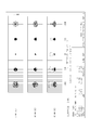
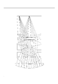
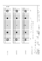
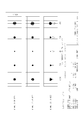
図3Bは、数値実施例1におけるスポットダイアグラムの像高およびデフォーカス依存性を示す。本図を参照すると、各像高において、デフォーカスに対してスポット径は比較的に一定の大きさを有していることがわかる。デフォーカス0において所定の広がりが認められることに注目されるべきである。なお、デフォーカス0の位置は、中心MTFの値がピークとなる光軸上の位置近傍において周辺性能とのバランスから決定される。
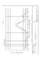
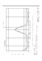
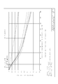
図3Cは、数値実施例1における深度対MTFを示す。本図を参照すると、MTFの最大値が約0.57程度と比較的に低くなっていることがわかる。また、MTFの分布が比較的に幅広になっており、デフォーカスした位置にも相当強度の応答を有することがわかる。
レンズ系の焦点深度は、多くの場合、深度対MTFの分布において、最大MTF値に対する所定割合(例えば、20%)の強度を持つ幅で評価される。本数値実施例1おいては、上記の比較的に低いMTF値に応じた感度で撮像することができるとともに、像復元処理では実質的にMTF値を持ち上げる処理が施される。したがって、このレンズ系110においても、最大MTF値に対して所定の値を有するMTF値において、焦点深度を評価することができる。本図に示されるようにMTFの分布が比較的に幅広になっていることから、本数値実施例においては比較的に長い焦点深度を有していることがわかる。実際の焦点深度の評価値については、他の数値実施例とともに後述する。
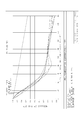
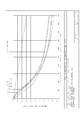
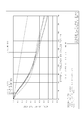
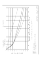
図3Dは、数値実施例1における空間周波数対MTFを、回折限界とともに示す。本図を参照すると、像高によらず比較的に一致した空間周波数対MTFを有することがわかる。このため、同じ復元処理パラメータを用いてもアーチファクトの発生を抑制することができる。また、本図から、比較的に高周波領域まで周波数応答を有することがわかる。このため、復元処理により高周波の信号を復元できることがわかる。
図4Aは、レンズ系110の他のレンズ構成を示す。表4には、図4Aに示すレンズ系110の数値実施例2の諸元の値を示す。
本数値実施例2における面番号12および面番号13の各ゾーンの諸元は、表5および表6に示される。表5および表6の諸元は、表2および表3の諸元と同様であるので、説明を省略する。以後説明する数値実施例の各ゾーンの諸元についても同様の諸元が示される。


図4B~図4Dには、数値実施例2の結像特性として、スポットダイアグラム図およびMTF特性が示されている。図4Bは、数値実施例2におけるスポットダイアグラムの像高およびデフォーカス依存性を示す。本図を参照して、デフォーカス0において所定の広がりが認められることに注目されるべきである。
図4Cは、数値実施例2における深度対MTFを示す。本図を参照すると、MTFの最大値が約0.57程度と比較的に低くなっており、MTFの分布が比較的に幅広になっていることがわかる。したがって、比較的に深い焦点深度を有することがわかる。
図4Dは、数値実施例2における空間周波数対MTFを、回折限界とともに示す。本図を参照すると、像高によらず比較的に一致した空間周波数対MTFを有することがわかる。また、比較的に高周波領域まで周波数応答を有することがわかる。
図4Dは、数値実施例1における空間周波数対MTFを、回折限界とともに示す。比較的に高周波領域まで周波数応答を有することがわかる。このため、復元処理により高周波の信号を復元できることがわかる。
図5Aは、レンズ系110の更なる他のレンズ構成を示す。表7には、図5Aに示すレンズ系110の数値実施例3の諸元の値を示す。
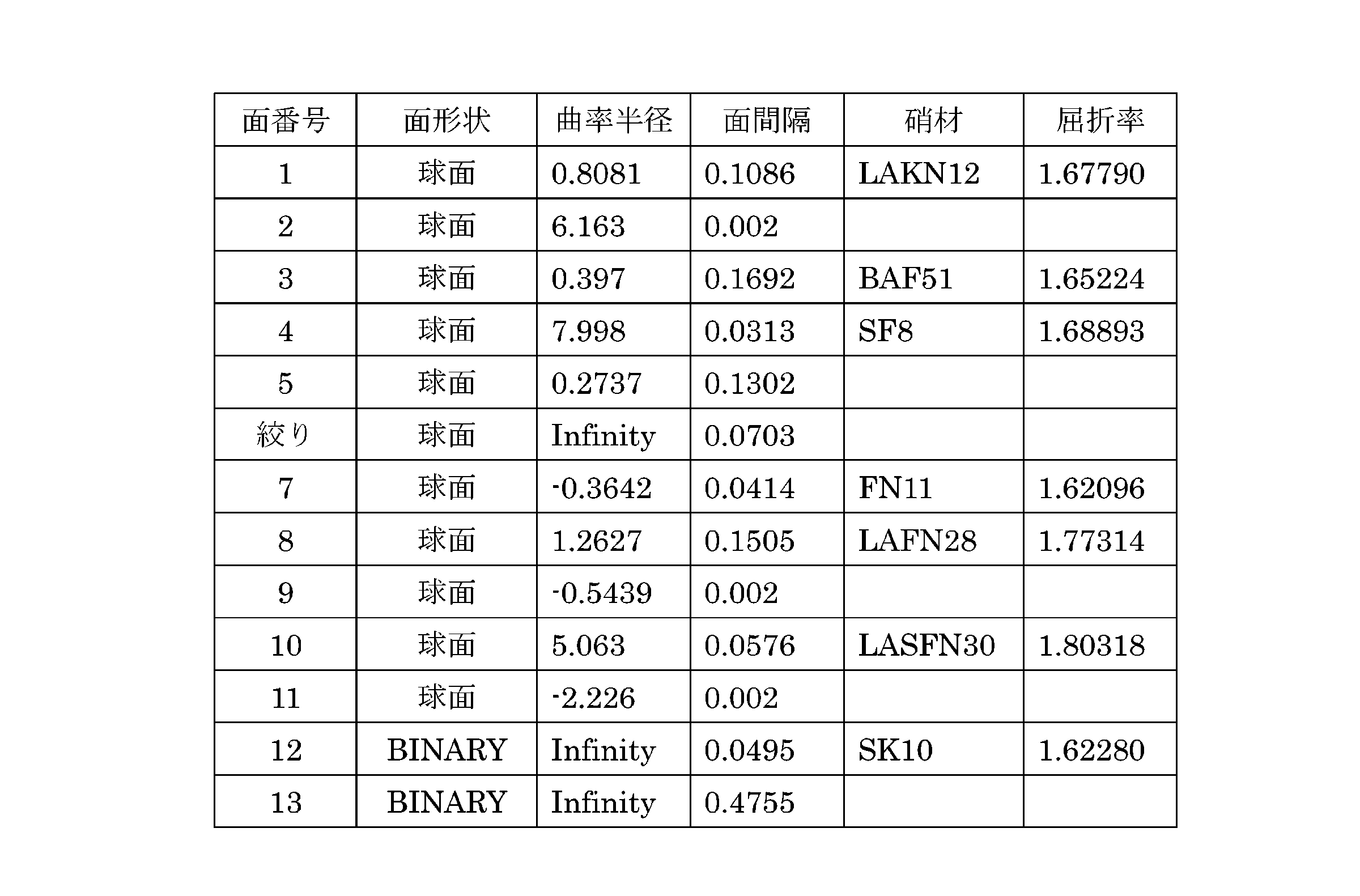
本数値実施例3における面番号12および面番号13の各ゾーンの諸元は、表8および表9に示される。


図5B~図5Dには、数値実施例4の結像特性として、スポットダイアグラム図およびMTF特性が示されている。図5Bは、数値実施例4におけるスポットダイアグラムの像高およびデフォーカス依存性を示す。本図を参照して、デフォーカス0においてスポットダイアグラムの所定の広がりが認められることに注目されるべきである。
図5Cは、数値実施例4における深度対MTFを示す。本図を参照すると、MTFの最大値が約0.46程度と比較的に低くなっており、MTFの分布が比較的に幅広になっていることがわかる。したがって、比較的に深い焦点深度を有することがわかる。
図5Dは、数値実施例4における空間周波数対MTFを、回折限界とともに示す。本図を参照すると、像高によらず比較的に一致した空間周波数対MTFを有することがわかる。また、比較的に高周波領域まで周波数応答を有することがわかる。
図6Aは、レンズ系110の更なる他のレンズ構成を示す。表10には、図6Aに示すレンズ系110の数値実施例4の諸元の値を示す。
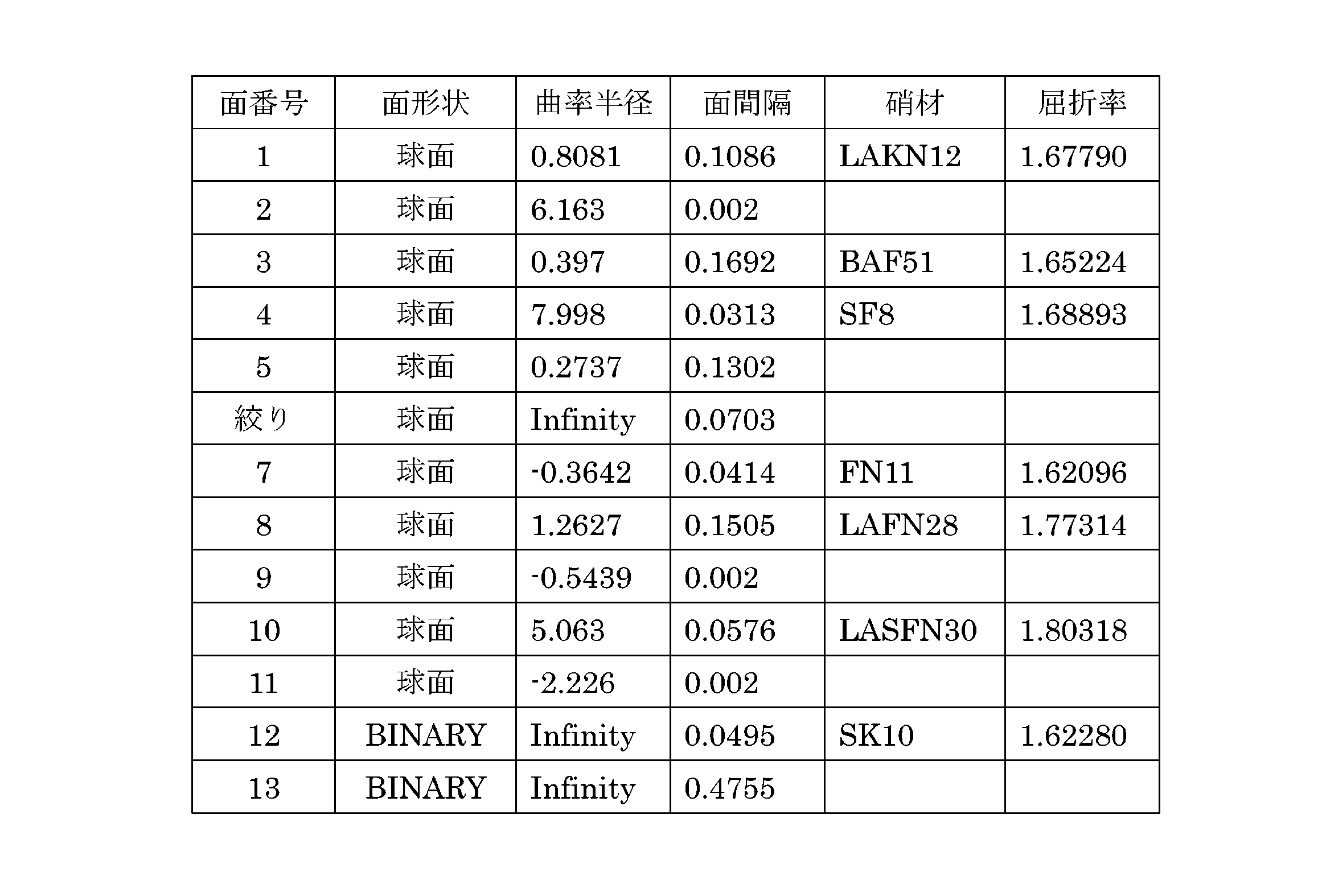
本数値実施例4における面番号12および面番号13の各ゾーンの諸元は、表11および表12に示される。


図6B~図6Dには、数値実施例4の結像特性として、スポットダイアグラム図およびMTF特性が示されている。図6Bは、数値実施例4におけるスポットダイアグラムの像高およびデフォーカス依存性を示す。本図を参照して、デフォーカス0においてスポットダイアグラムの所定の広がりが認められることに注目されるべきである。
図6Cは、数値実施例4における深度対MTFを示す。本図を参照すると、MTFの最大値が約0.62程度と比較的に低くなっており、MTFの分布が比較的に幅広になっていることがわかる。したがって、比較的に深い焦点深度を有することがわかる。
図6Dは、数値実施例5における空間周波数対MTFを、回折限界とともに示す。本図を参照すると、像高によらず比較的に一致した空間周波数対MTFを有することがわかる。また、比較的に高周波領域まで周波数応答を有することがわかる。
図7Aは、レンズ系110の更なる他のレンズ構成を示す。表10には、図7Aに示すレンズ系110の数値実施例5の諸元の値を示す。
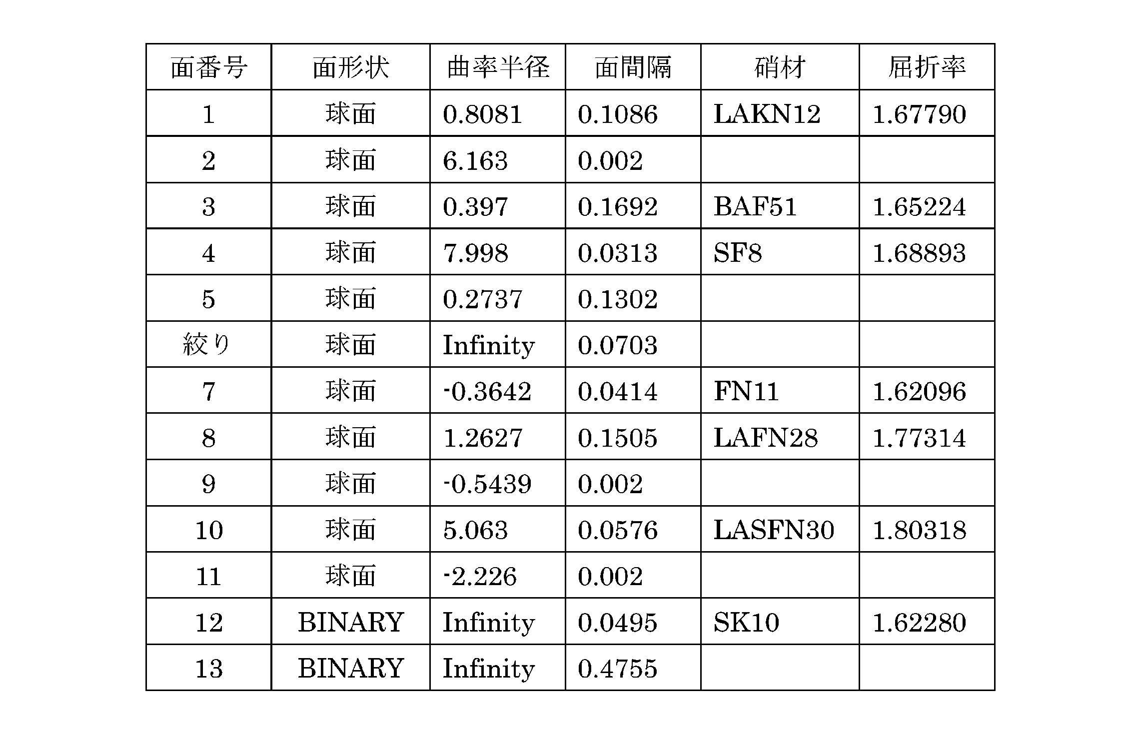
本数値実施例5における面番号12および面番号13の各ゾーンの諸元は、表14および表15に示される。
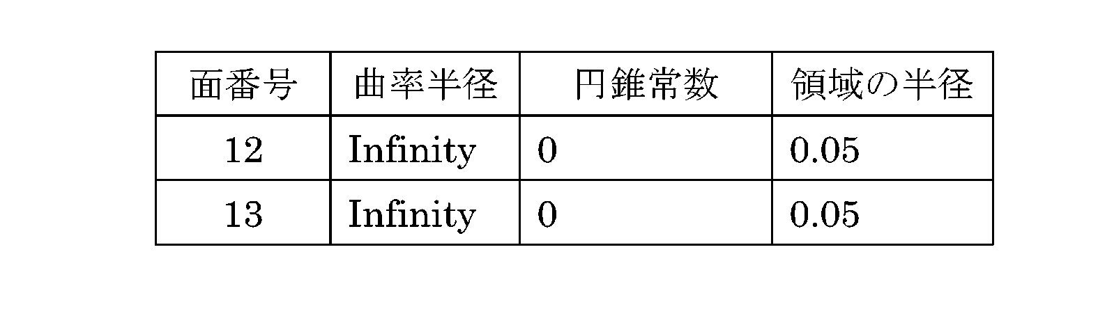

図7B~図7Dには、数値実施例5の結像特性として、スポットダイアグラム図およびMTF特性が示されている。図7Bは、数値実施例5におけるスポットダイアグラムの像高およびデフォーカス依存性を示す。本図を参照して、デフォーカス0においてスポットダイアグラムの所定の広がりが認められることに注目されるべきである。
図7Cは、数値実施例5における深度対MTFを示す。本図を参照すると、MTFの最大値が約0.65程度と比較的に低くなっており、MTFの分布が比較的に幅広になっていることがわかる。したがって、比較的に深い焦点深度を有することがわかる。
図7Dは、数値実施例5における空間周波数対MTFを、回折限界とともに示す。本図を参照すると、像高によらず比較的に一致した空間周波数対MTFを有することがわかる。また、比較的に高周波領域まで周波数応答を有することがわかる。
図8Aは、レンズ系110の更なる他のレンズ構成を示す。表16には、図8Aに示すレンズ系110の数値実施例6の諸元の値を示す。

本数値実施例6における面番号1および面番号2の各ゾーンの諸元は、表17および表18に示される。

本数値実施例6における非球面の面番号5-12の非球面データは、表19A~表19Dに示される。なお、非球面の面番号に対応する曲率半径の欄には、非球面の面形状を規定する一パラメータである基準曲率半径が記載される。


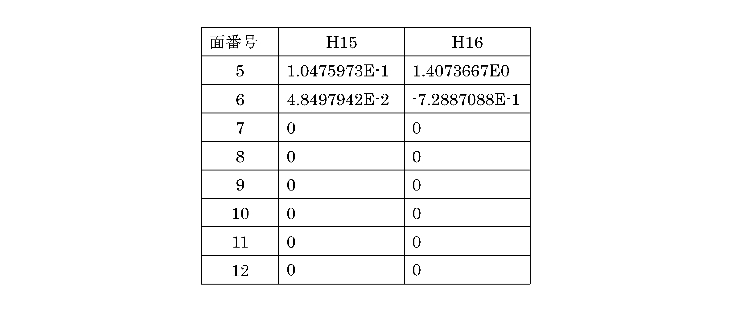
図8B~図8Dには、数値実施例6の結像特性として、スポットダイアグラム図およびMTF特性が示されている。図8Bは、数値実施例6におけるスポットダイアグラムの像高およびデフォーカス依存性を示す。本図を参照して、デフォーカス0においてスポットダイアグラムの所定の広がりが認められることに注目されるべきである。
図8Cは、数値実施例6における深度対MTFを示す。本図を参照すると、MTFの最大値が約0.52程度と比較的に低くなっており、MTFの分布が比較的に幅広になっていることがわかる。したがって、比較的に深い焦点深度を有することがわかる。
図8Dは、数値実施例6における空間周波数対MTFを、回折限界とともに示す。本図を参照すると、像高によらず比較的に一致した空間周波数対MTFを有することがわかる。また、比較的に高周波領域まで周波数応答を有することがわかる。このため、復元処理により高周波の信号を復元できることができることがわかる。
本数値実施例6では、平坦領域は最も物体側に位置するレンズに形成されている。最も像側に位置するレンズに平坦領域が形成されなくとも、比較的に深い焦点深度を有するレンズ系を設計することができる。光軸を含まない領域では元々収差が存在しており、レンズ設計において光軸を含む領域よりも比較的に結像特性を制御し易い。このため、光軸を含む所定の良否域が平坦な場合であっても、平坦領域の周囲の領域の光学パラメータを適切に設計することで、スポットの広がりを略一定にすることができる場合がある。
図9Aは、レンズ系110の更なる他のレンズ構成を示す。表20には、図9Aに示すレンズ系110の数値実施例7の諸元の値を示す。なお、面番号12の光学面は、光軸から半径0.025mm以内のゾーンは多項式で定められ、その周囲のゾーンは、半径0.08mmの非球面となっている。

本数値実施例7における面番号12の各ゾーンの諸元は、表21に示される。
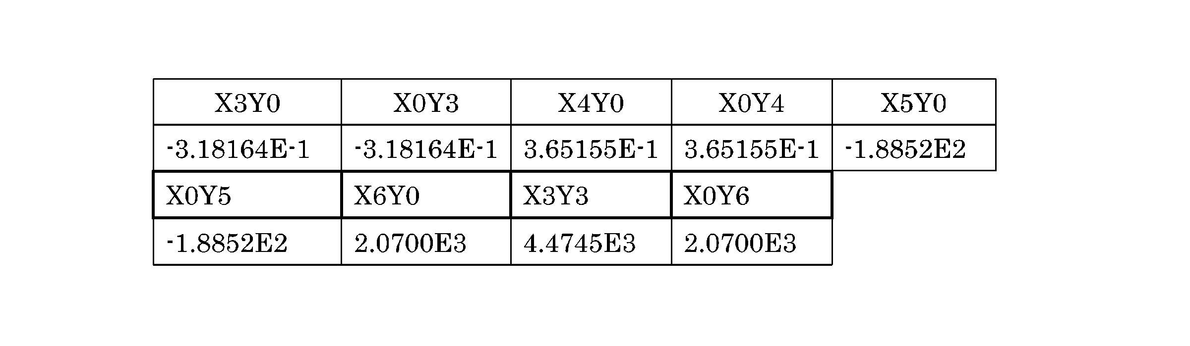
XnYmに対応する欄には、光軸を原点としてx座標についてn次、y座標についてm次の次数の項に対する係数が示されている。すなわち、光学面のザグzは、以下の式で表される。

上式を展開すると以下ように表される。

上式の係数Aiが、表21の各欄の係数に対応する。
本数値実施例7における非球面の面番号3-12の非球面データは、表22A~表22Dに示される。
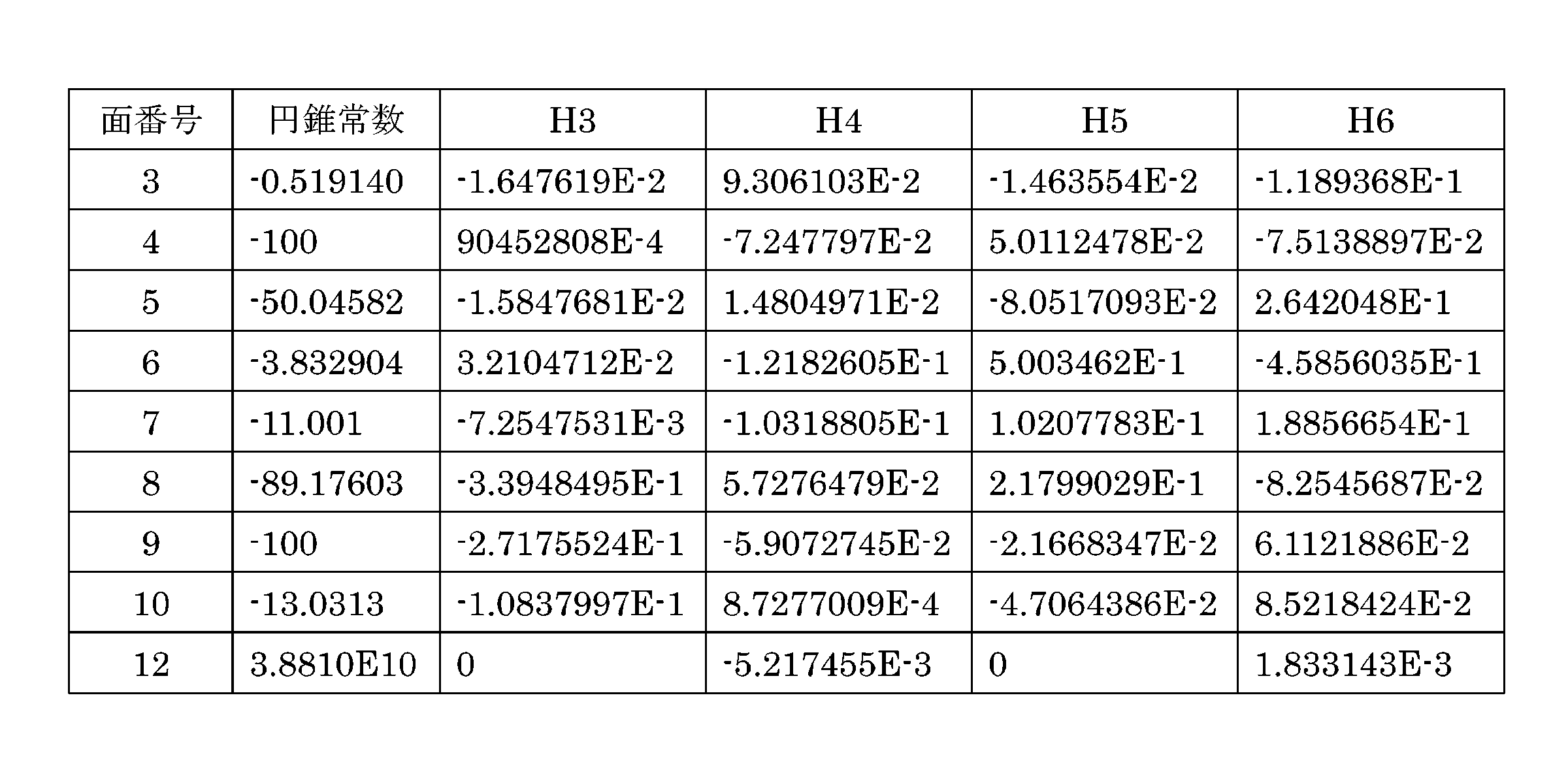
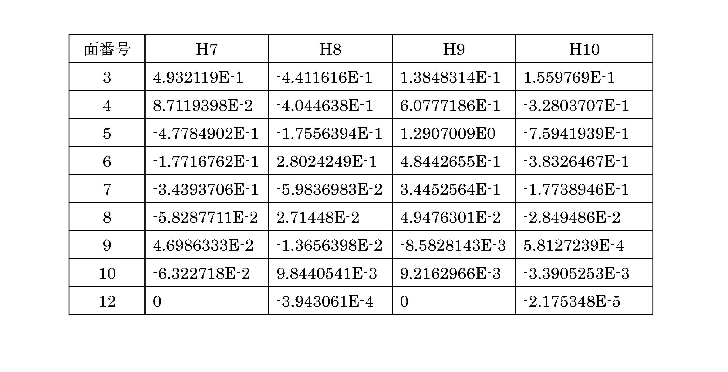

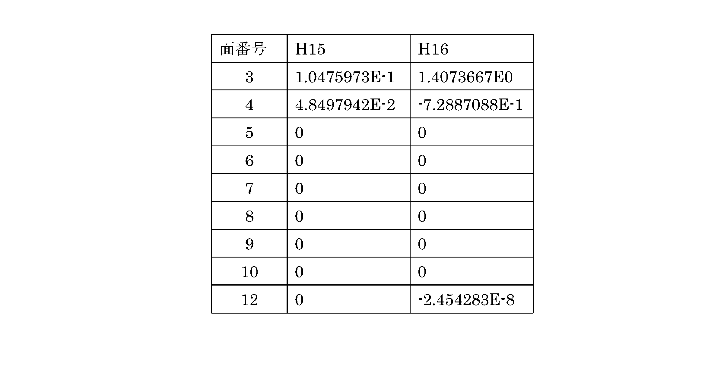
図9B~図9Dには、数値実施例7の結像特性として、スポットダイアグラム図およびMTF特性が示されている。図9Bは、数値実施例7におけるスポットダイアグラムの像高およびデフォーカス依存性を示す。本図を参照して、デフォーカス0においてスポットダイアグラムの所定の広がりが認められることに注目されるべきである。
図9Cは、数値実施例7における深度対MTFを示す。本図を参照すると、MTFの最大値が約0.72程度と比較的に低くなっており、MTFの分布が比較的に幅広になっていることがわかる。したがって、比較的に深い焦点深度を有することがわかる。
図9Dは、数値実施例7における空間周波数対MTFを、回折限界とともに示す。本図を参照すると、比較的に高周波領域まで周波数応答を有することがわかる。このため、復元処理により高周波の信号を復元できることができることがわかる。
本数値実施例7から、光軸近傍の領域が平坦面でなくとも、比較的に深い焦点深度を有するレンズ系を設計できることがわかる。
ここで参考のため、数値実施例1-7に係るレンズ系において低結像部を有しないレンズ構成の実施例を示す。図10Aには、数値実施例1-5に係るレンズ系に対応するレンズ系を示す。表23には、図10Aに示すレンズ系110の数値実施例の諸元の値を示す。

図10B~図10Dには、本数値実施例の結像特性として、スポットダイアグラム図およびMTF特性が示されている。図10Bは、本数値実施例におけるスポットダイアグラムの像高およびデフォーカス依存性を示す。本図を参照すると、デフォーカス0においてスポットダイアグラムが比較的に小さいことがわかる。また、数値実施例1-5に係るレンズ系と比べると、デフォーカス依存性が著しく大きいことがわかる。
図10Cは、本数値実施例における深度対MTFを示す。本図を参照すると、MTFの最大値が約0.86程度と比較的に高くなっており、MTFの分布が比較的に幅狭になっていることがわかる。したがって、焦点深度は比較的に狭いことがわかる。
図10Dは、本数値実施例における空間周波数対MTFを、回折限界とともに示す。本図を参照すると、近軸光に対しては回折限界に近い周波数応答を有することがわかる。しかしながら、異なる像高に対して周波数応答が比較的に大きく異なっていることがわかる。
以上数値実施例1-7に例示したように、光軸を含む中央領域に低結像部を形成することにより、比較的に深い焦点深度を持つ光学系を設計することができることが示された。
表24Aおよび表24Bは、上記数値実施例において低結像部の径を異ならせた場合の焦点深度を示す。
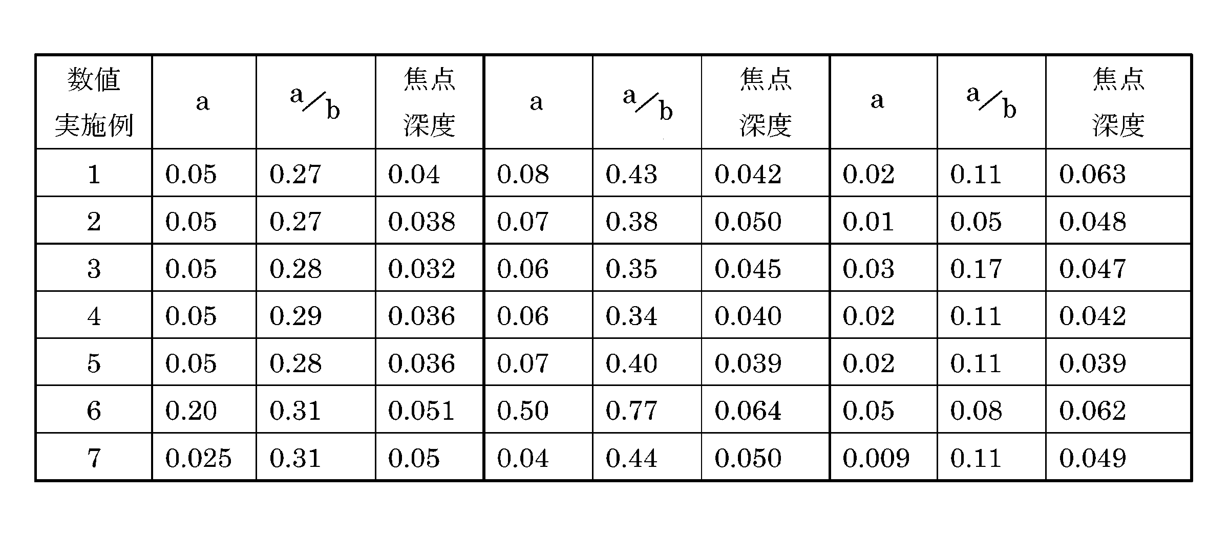
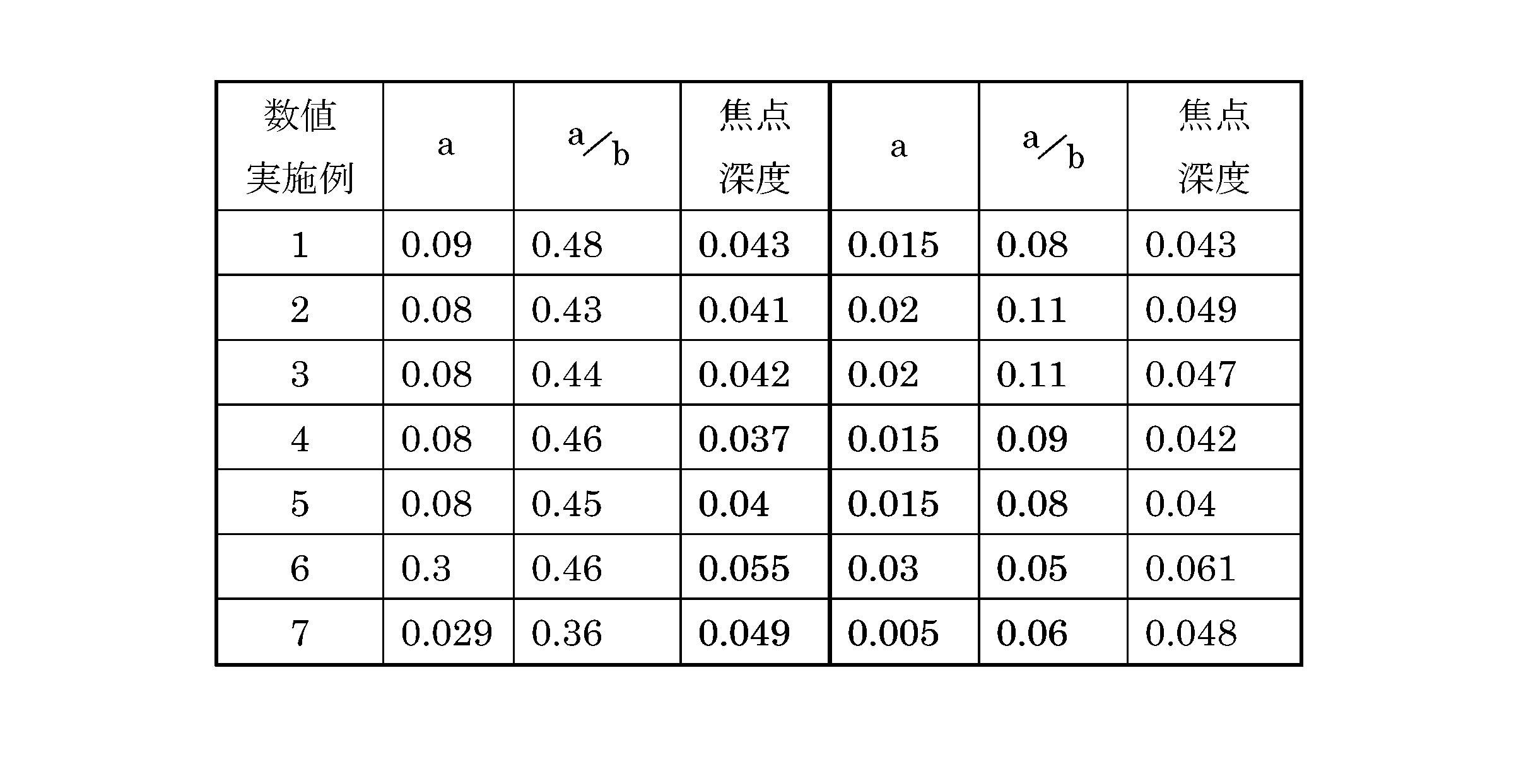
本表は、数値実施例の番号、低結像部の高さ(a)、第1指標値(a/b)、および、焦点深度が示されている。第1指標値は、低結像部を有するレンズを通過する軸上光線の最大高さ(b)と低結像部の高さの比(a/b)で定めるとする。深度対MTF値のMTF分布において、MTF値が所定の評価基準MTF値となる幅を、焦点深度とした。評価基準MTF値には、およそ最大MTF値の20%となる値にとった。
本表に示すように、いずれの大きさのaについても、比較的に深い焦点深度が得られた。ここで第1指標値a/bが0.05以上0.77以下の場合に、比較的に深い焦点深度が得られた。焦点深度を深くすることを目的とした場合に、第1指標値を0.05以上0.77以下とすることがよい。
また、第1指標値が0.08以上0.60以下である場合には、数値実施例1~7のより多くの光学系の場合において比較的に長い焦点深度が得られている。すなわち、焦点深度を深くすることを目的とした場合に、第1指標値を0.08以上0.60以下とすることが望ましいといえる。
特に、第1指標値が0.11以上0.43以下である場合に、数値実施例1~7のより多くの光学系の場合において、比較的に長い焦点深度が得られている。すなわち、焦点深度を深くすることを目的とした場合に、第1指標値を0.11以上0.43以下とすることがより望ましいといえる。
表25は、上記数値実施例において焦点深度に影響を与える第2指標値を示す。本表には、数値実施例の番号、低結像部を含む領域の焦点距離(f1)、低結像部を含む領域のバックフォーカス(fb1)、低結像部を含まない領域の基準曲率半径に対応する焦点距離(f2)、当該基準曲率半径に対応するバックフォーカス(fb2)、入射瞳径、Fナンバー(FN)、および、第2指標値を示す。

第2指標値は、(fb2/fb1)×FNで定めるとする。上記数値実施例1-7において、第2指標値が2.4から2.87までの間で、深い焦点深度が得られた。すなわち、焦点深度を深くすることを目的とした場合に、第2指標値は2.4以上2.87以下の範囲内であることが好ましい。
以上この発明の実施例として、低結像領域が、最も像側の第1レンズの像側の面および最も像側位置するレンズに設けたものを例示した。しかし、当該低結像領域の位置は当該箇所に限定されるものではない。低結像領域を有する面の位置にかかわらず、この発明の所定の範囲を満足する限り、光軸上の性能に関しては同じ効果が得られる。一方、絞りから離れた位置に低結像領域がある場合、低結像領域は主に光軸近傍の結像特性に対して影響を及ぼし、低結像領の位置が絞りに近づくほど低結像領域の影響が周辺性能へも影響を及ぼすようになるので、周辺性能とのバランスを考慮して、低結像領の位置を適宜選択することが可能である。
以上、本発明を実施の形態を用いて説明したが、本発明の技術的範囲は上記実施の形態に記載の範囲には限定されない。上記実施の形態に、多様な変更または改良を加えることが可能であることが当業者に明らかである。その様な変更または改良を加えた形態も本発明の技術的範囲に含まれ得ることが、請求の範囲の記載から明らかである。
請求の範囲、明細書、および図面中において示した装置、システム、プログラム、および方法における動作、手順、ステップ、および段階等の各処理の実行順序は、特段「より前に」、「先立って」等と明示しておらず、また、前の処理の出力を後の処理で用いるのでない限り、任意の順序で実現しうることに留意すべきである。請求の範囲、明細書、および図面中の動作フローに関して、便宜上「まず、」、「次に、」等を用いて説明したとしても、この順で実施することが必須であることを意味するものではない。
110 レンズ系
100 撮像装置
115 レンズ
120 受光部
140 補正部
145 画像処理部
150 出力部
210 光線
220 光線
230 光線
260 低結像領域
100 撮像装置
115 レンズ
120 受光部
140 補正部
145 画像処理部
150 出力部
210 光線
220 光線
230 光線
260 低結像領域
Claims (15)
- 他の領域の光学パラメータが与える結像特性よりも低い結像特性を与える光学パラメータを有する低結像部を有し、
前記低結像部および前記他の領域を通過する物点からの光に対する光学伝達関数が、物点までの距離によらず略同一である
光学系。 - 前記光学系は、前記低結像部および前記他の領域を通過する物点からの光を、物点までの距離によらず略同一の大きさに広げる
請求項1に記載の光学系。 - 前記低結像部は、光軸を含む領域であり、前記他の領域は、前記低結像部の周囲の光軸を含まない領域である
請求項1または2に記載の光学系。 - 前記低結像部は、前記光学系が有する少なくとも1のレンズの少なくとも1の面の前記光軸を含む一部領域に形成され、当該面の前記光軸を含まない領域の光学パラメータが与える結像特性よりも低い結像特性を与える光学パラメータを有する
請求項3に記載の光学系。 - 前記低結像部は、前記光軸を含まない領域の曲面形状が与える結像特性よりも低い結像特性を与える曲面形状を有する
請求項4に記載の光学系。 - 前記低結像部の基準曲率半径は、前記他の領域の基準曲率半径より大きい
請求項5に記載の光学系。 - 前記低結像部の基準曲率半径は実質的に無限大である
請求項5に記載の光学系。 - 前記低結像部は、像面に最も近いレンズの像側の光学面に形成される
請求項7に記載の光学系。 - 前記低結像部は、最も物体側に位置するレンズに形成される
請求項7に記載の光学系。 - 前記低結像部の高さaと、前記低結像部を有する面を軸上光線が通過する最大高さbとが、
0.05≦a/b≦0.77
を満たす請求項6に記載の光学系。 - 前記aと、前記bとが、
0.08≦a/b≦0.60
を満たす請求項10に記載の光学系。 - 前記aと、前記bとが、
0.11≦a/b≦0.43
を満たす請求項11に記載の光学系。 - 前記低結像部における曲面形状によるバックフォーカスの値fb1、前記他の領域の曲面形状によるバックフォーカスの値fb2、および、前記光学系のFナンバーの値FNが、
2.4≦(fb2/fb1)×FN≦2.87
を満たす請求項6に記載の光学系。 - 請求項1から13のいずれかに記載の光学系と、
前記光学系を通過した光を受光する受光部と
を備える撮像装置。 - 前記受光部は、複数の画素にそれぞれ対応する複数の受光素子を有し、前記複数の画素はそれぞれ少なくとも3色のカラーフィルタの1色を透過した光を受光し、
前記光学系は、前記3色の光を受光する近接した3個の画素より形成される画素ブロックより大きく広げたことを特徴とする
請求項14に記載の撮像装置。
Applications Claiming Priority (2)
| Application Number | Priority Date | Filing Date | Title |
|---|---|---|---|
| JP2009167303A JP2011022358A (ja) | 2009-07-15 | 2009-07-15 | 光学系および撮像装置 |
| JP2009-167303 | 2009-07-15 |
Publications (1)
| Publication Number | Publication Date |
|---|---|
| WO2011007485A1 true WO2011007485A1 (ja) | 2011-01-20 |
Family
ID=43449097
Family Applications (1)
| Application Number | Title | Priority Date | Filing Date |
|---|---|---|---|
| PCT/JP2010/002986 Ceased WO2011007485A1 (ja) | 2009-07-15 | 2010-04-26 | 光学系および撮像装置 |
Country Status (2)
| Country | Link |
|---|---|
| JP (1) | JP2011022358A (ja) |
| WO (1) | WO2011007485A1 (ja) |
Families Citing this family (1)
| Publication number | Priority date | Publication date | Assignee | Title |
|---|---|---|---|---|
| JP2015004883A (ja) * | 2013-06-21 | 2015-01-08 | 株式会社リコー | 結像光学系および撮像システムおよび撮像方法 |
Citations (2)
| Publication number | Priority date | Publication date | Assignee | Title |
|---|---|---|---|---|
| JP2007122055A (ja) * | 2005-10-27 | 2007-05-17 | Samsung Electro-Mechanics Co Ltd | 多重曲率レンズを具備する光学システム及びその形成方法 |
| JP2009010783A (ja) * | 2007-06-28 | 2009-01-15 | Kyocera Corp | 撮像装置 |
-
2009
- 2009-07-15 JP JP2009167303A patent/JP2011022358A/ja not_active Withdrawn
-
2010
- 2010-04-26 WO PCT/JP2010/002986 patent/WO2011007485A1/ja not_active Ceased
Patent Citations (2)
| Publication number | Priority date | Publication date | Assignee | Title |
|---|---|---|---|---|
| JP2007122055A (ja) * | 2005-10-27 | 2007-05-17 | Samsung Electro-Mechanics Co Ltd | 多重曲率レンズを具備する光学システム及びその形成方法 |
| JP2009010783A (ja) * | 2007-06-28 | 2009-01-15 | Kyocera Corp | 撮像装置 |
Also Published As
| Publication number | Publication date |
|---|---|
| JP2011022358A (ja) | 2011-02-03 |
Similar Documents
| Publication | Publication Date | Title |
|---|---|---|
| US10359606B2 (en) | Optical image capturing system | |
| US8054368B2 (en) | Imaging system, imaging apparatus, portable terminal apparatus, onboard apparatus, and medical apparatus | |
| US9971127B2 (en) | Optical image capturing system | |
| US20180335609A1 (en) | Optical image capturing system | |
| US9217851B2 (en) | Zoom lens and image pickup device including the same | |
| US9989738B2 (en) | Optical image capturing system | |
| US9897781B2 (en) | Optical image capturing system | |
| US10095006B2 (en) | Optical image capturing system | |
| US9651722B2 (en) | Optical system and optical apparatus | |
| US20180188492A1 (en) | Optical image capturing system | |
| CN107589534B (zh) | 一种透镜系统及镜头 | |
| US11480763B2 (en) | Optical image capturing system | |
| JP2015203850A (ja) | 赤外線撮像装置 | |
| US10268020B2 (en) | Optical image capturing system | |
| US11221459B2 (en) | Imaging optical system and imaging apparatus | |
| JP4796666B2 (ja) | 撮像装置およびそれを用いた測距装置 | |
| US20190278054A1 (en) | Optical image capturing system | |
| JP2009169092A (ja) | 光学系および撮像装置 | |
| WO2020017258A1 (ja) | レンズ系、撮像装置及び撮像システム | |
| US10877249B2 (en) | Optical image capturing system | |
| US20210223511A1 (en) | Optical image capturing system | |
| US10338346B2 (en) | Optical image capturing system | |
| JP2019124823A5 (ja) | 撮像光学系および撮像装置 | |
| JP2018106159A (ja) | フルフレームセンサを有するカメラの最高撮像品質のコンパクトカメラレンズ | |
| CN100394803C (zh) | 色差校正成像光学系统 |
Legal Events
| Date | Code | Title | Description |
|---|---|---|---|
| 121 | Ep: the epo has been informed by wipo that ep was designated in this application |
Ref document number: 10799549 Country of ref document: EP Kind code of ref document: A1 |
|
| NENP | Non-entry into the national phase |
Ref country code: DE |
|
| 122 | Ep: pct application non-entry in european phase |
Ref document number: 10799549 Country of ref document: EP Kind code of ref document: A1 |