EP3716200A1 - Image processing apparatus and method for use in an autofocus system - Google Patents
Image processing apparatus and method for use in an autofocus system Download PDFInfo
- Publication number
- EP3716200A1 EP3716200A1 EP19194731.6A EP19194731A EP3716200A1 EP 3716200 A1 EP3716200 A1 EP 3716200A1 EP 19194731 A EP19194731 A EP 19194731A EP 3716200 A1 EP3716200 A1 EP 3716200A1
- Authority
- EP
- European Patent Office
- Prior art keywords
- image
- input
- output
- images
- baseline estimate
- Prior art date
- Legal status (The legal status is an assumption and is not a legal conclusion. Google has not performed a legal analysis and makes no representation as to the accuracy of the status listed.)
- Granted
Links
Images


Classifications
-
- G—PHYSICS
- G06—COMPUTING OR CALCULATING; COUNTING
- G06T—IMAGE DATA PROCESSING OR GENERATION, IN GENERAL
- G06T5/00—Image enhancement or restoration
- G06T5/73—Deblurring; Sharpening
-
- G—PHYSICS
- G02—OPTICS
- G02B—OPTICAL ELEMENTS, SYSTEMS OR APPARATUS
- G02B21/00—Microscopes
- G02B21/06—Means for illuminating specimens
- G02B21/08—Condensers
- G02B21/12—Condensers affording bright-field illumination
-
- G—PHYSICS
- G02—OPTICS
- G02B—OPTICAL ELEMENTS, SYSTEMS OR APPARATUS
- G02B21/00—Microscopes
- G02B21/24—Base structure
- G02B21/241—Devices for focusing
- G02B21/244—Devices for focusing using image analysis techniques
-
- G—PHYSICS
- G02—OPTICS
- G02B—OPTICAL ELEMENTS, SYSTEMS OR APPARATUS
- G02B7/00—Mountings, adjusting means, or light-tight connections, for optical elements
- G02B7/28—Systems for automatic generation of focusing signals
- G02B7/36—Systems for automatic generation of focusing signals using image sharpness techniques, e.g. image processing techniques for generating autofocus signals
- G02B7/38—Systems for automatic generation of focusing signals using image sharpness techniques, e.g. image processing techniques for generating autofocus signals measured at different points on the optical axis, e.g. focussing on two or more planes and comparing image data
-
- G—PHYSICS
- G03—PHOTOGRAPHY; CINEMATOGRAPHY; ANALOGOUS TECHNIQUES USING WAVES OTHER THAN OPTICAL WAVES; ELECTROGRAPHY; HOLOGRAPHY
- G03B—APPARATUS OR ARRANGEMENTS FOR TAKING PHOTOGRAPHS OR FOR PROJECTING OR VIEWING THEM; APPARATUS OR ARRANGEMENTS EMPLOYING ANALOGOUS TECHNIQUES USING WAVES OTHER THAN OPTICAL WAVES; ACCESSORIES THEREFOR
- G03B13/00—Viewfinders; Focusing aids for cameras; Means for focusing for cameras; Autofocus systems for cameras
- G03B13/32—Means for focusing
- G03B13/34—Power focusing
- G03B13/36—Autofocus systems
-
- G—PHYSICS
- G06—COMPUTING OR CALCULATING; COUNTING
- G06F—ELECTRIC DIGITAL DATA PROCESSING
- G06F17/00—Digital computing or data processing equipment or methods, specially adapted for specific functions
- G06F17/10—Complex mathematical operations
- G06F17/11—Complex mathematical operations for solving equations, e.g. nonlinear equations, general mathematical optimization problems
- G06F17/13—Differential equations
-
- G—PHYSICS
- G06—COMPUTING OR CALCULATING; COUNTING
- G06F—ELECTRIC DIGITAL DATA PROCESSING
- G06F17/00—Digital computing or data processing equipment or methods, specially adapted for specific functions
- G06F17/10—Complex mathematical operations
- G06F17/15—Correlation function computation including computation of convolution operations
-
- G—PHYSICS
- G06—COMPUTING OR CALCULATING; COUNTING
- G06T—IMAGE DATA PROCESSING OR GENERATION, IN GENERAL
- G06T5/00—Image enhancement or restoration
- G06T5/10—Image enhancement or restoration using non-spatial domain filtering
-
- G—PHYSICS
- G06—COMPUTING OR CALCULATING; COUNTING
- G06T—IMAGE DATA PROCESSING OR GENERATION, IN GENERAL
- G06T5/00—Image enhancement or restoration
- G06T5/20—Image enhancement or restoration using local operators
-
- G—PHYSICS
- G06—COMPUTING OR CALCULATING; COUNTING
- G06T—IMAGE DATA PROCESSING OR GENERATION, IN GENERAL
- G06T5/00—Image enhancement or restoration
- G06T5/60—Image enhancement or restoration using machine learning, e.g. neural networks
-
- G—PHYSICS
- G06—COMPUTING OR CALCULATING; COUNTING
- G06T—IMAGE DATA PROCESSING OR GENERATION, IN GENERAL
- G06T5/00—Image enhancement or restoration
- G06T5/70—Denoising; Smoothing
-
- G—PHYSICS
- G06—COMPUTING OR CALCULATING; COUNTING
- G06T—IMAGE DATA PROCESSING OR GENERATION, IN GENERAL
- G06T7/00—Image analysis
- G06T7/0002—Inspection of images, e.g. flaw detection
- G06T7/0012—Biomedical image inspection
-
- G—PHYSICS
- G06—COMPUTING OR CALCULATING; COUNTING
- G06V—IMAGE OR VIDEO RECOGNITION OR UNDERSTANDING
- G06V10/00—Arrangements for image or video recognition or understanding
- G06V10/20—Image preprocessing
- G06V10/30—Noise filtering
-
- H—ELECTRICITY
- H04—ELECTRIC COMMUNICATION TECHNIQUE
- H04L—TRANSMISSION OF DIGITAL INFORMATION, e.g. TELEGRAPHIC COMMUNICATION
- H04L25/00—Baseband systems
- H04L25/02—Details ; arrangements for supplying electrical power along data transmission lines
- H04L25/0202—Channel estimation
- H04L25/024—Channel estimation channel estimation algorithms
- H04L25/025—Channel estimation channel estimation algorithms using least-mean-square [LMS] method
-
- H—ELECTRICITY
- H04—ELECTRIC COMMUNICATION TECHNIQUE
- H04N—PICTORIAL COMMUNICATION, e.g. TELEVISION
- H04N23/00—Cameras or camera modules comprising electronic image sensors; Control thereof
- H04N23/60—Control of cameras or camera modules
- H04N23/67—Focus control based on electronic image sensor signals
- H04N23/675—Focus control based on electronic image sensor signals comprising setting of focusing regions
-
- H—ELECTRICITY
- H04—ELECTRIC COMMUNICATION TECHNIQUE
- H04N—PICTORIAL COMMUNICATION, e.g. TELEVISION
- H04N25/00—Circuitry of solid-state image sensors [SSIS]; Control thereof
- H04N25/60—Noise processing, e.g. detecting, correcting, reducing or removing noise
- H04N25/61—Noise processing, e.g. detecting, correcting, reducing or removing noise the noise originating only from the lens unit, e.g. flare, shading, vignetting or "cos4"
- H04N25/615—Noise processing, e.g. detecting, correcting, reducing or removing noise the noise originating only from the lens unit, e.g. flare, shading, vignetting or "cos4" involving a transfer function modelling the optical system, e.g. optical transfer function [OTF], phase transfer function [PhTF] or modulation transfer function [MTF]
-
- G—PHYSICS
- G01—MEASURING; TESTING
- G01S—RADIO DIRECTION-FINDING; RADIO NAVIGATION; DETERMINING DISTANCE OR VELOCITY BY USE OF RADIO WAVES; LOCATING OR PRESENCE-DETECTING BY USE OF THE REFLECTION OR RERADIATION OF RADIO WAVES; ANALOGOUS ARRANGEMENTS USING OTHER WAVES
- G01S13/00—Systems using the reflection or reradiation of radio waves, e.g. radar systems; Analogous systems using reflection or reradiation of waves whose nature or wavelength is irrelevant or unspecified
- G01S13/88—Radar or analogous systems specially adapted for specific applications
- G01S13/89—Radar or analogous systems specially adapted for specific applications for mapping or imaging
-
- G—PHYSICS
- G01—MEASURING; TESTING
- G01S—RADIO DIRECTION-FINDING; RADIO NAVIGATION; DETERMINING DISTANCE OR VELOCITY BY USE OF RADIO WAVES; LOCATING OR PRESENCE-DETECTING BY USE OF THE REFLECTION OR RERADIATION OF RADIO WAVES; ANALOGOUS ARRANGEMENTS USING OTHER WAVES
- G01S15/00—Systems using the reflection or reradiation of acoustic waves, e.g. sonar systems
- G01S15/88—Sonar systems specially adapted for specific applications
- G01S15/89—Sonar systems specially adapted for specific applications for mapping or imaging
-
- G—PHYSICS
- G01—MEASURING; TESTING
- G01S—RADIO DIRECTION-FINDING; RADIO NAVIGATION; DETERMINING DISTANCE OR VELOCITY BY USE OF RADIO WAVES; LOCATING OR PRESENCE-DETECTING BY USE OF THE REFLECTION OR RERADIATION OF RADIO WAVES; ANALOGOUS ARRANGEMENTS USING OTHER WAVES
- G01S7/00—Details of systems according to groups G01S13/00, G01S15/00, G01S17/00
- G01S7/02—Details of systems according to groups G01S13/00, G01S15/00, G01S17/00 of systems according to group G01S13/00
- G01S7/41—Details of systems according to groups G01S13/00, G01S15/00, G01S17/00 of systems according to group G01S13/00 using analysis of echo signal for target characterisation; Target signature; Target cross-section
- G01S7/417—Details of systems according to groups G01S13/00, G01S15/00, G01S17/00 of systems according to group G01S13/00 using analysis of echo signal for target characterisation; Target signature; Target cross-section involving the use of neural networks
-
- G—PHYSICS
- G01—MEASURING; TESTING
- G01V—GEOPHYSICS; GRAVITATIONAL MEASUREMENTS; DETECTING MASSES OR OBJECTS; TAGS
- G01V1/00—Seismology; Seismic or acoustic prospecting or detecting
- G01V1/28—Processing seismic data, e.g. for interpretation or for event detection
- G01V1/36—Effecting static or dynamic corrections on records, e.g. correcting spread; Correlating seismic signals; Eliminating effects of unwanted energy
-
- G—PHYSICS
- G02—OPTICS
- G02B—OPTICAL ELEMENTS, SYSTEMS OR APPARATUS
- G02B21/00—Microscopes
- G02B21/06—Means for illuminating specimens
- G02B21/08—Condensers
- G02B21/086—Condensers for transillumination only
-
- G—PHYSICS
- G02—OPTICS
- G02B—OPTICAL ELEMENTS, SYSTEMS OR APPARATUS
- G02B21/00—Microscopes
- G02B21/24—Base structure
- G02B21/241—Devices for focusing
-
- G—PHYSICS
- G02—OPTICS
- G02B—OPTICAL ELEMENTS, SYSTEMS OR APPARATUS
- G02B21/00—Microscopes
- G02B21/36—Microscopes arranged for photographic purposes or projection purposes or digital imaging or video purposes including associated control and data processing arrangements
- G02B21/365—Control or image processing arrangements for digital or video microscopes
-
- G—PHYSICS
- G02—OPTICS
- G02B—OPTICAL ELEMENTS, SYSTEMS OR APPARATUS
- G02B3/00—Simple or compound lenses
- G02B3/12—Fluid-filled or evacuated lenses
- G02B3/14—Fluid-filled or evacuated lenses of variable focal length
-
- G—PHYSICS
- G06—COMPUTING OR CALCULATING; COUNTING
- G06T—IMAGE DATA PROCESSING OR GENERATION, IN GENERAL
- G06T2207/00—Indexing scheme for image analysis or image enhancement
- G06T2207/10—Image acquisition modality
- G06T2207/10056—Microscopic image
-
- G—PHYSICS
- G06—COMPUTING OR CALCULATING; COUNTING
- G06T—IMAGE DATA PROCESSING OR GENERATION, IN GENERAL
- G06T2207/00—Indexing scheme for image analysis or image enhancement
- G06T2207/10—Image acquisition modality
- G06T2207/10068—Endoscopic image
-
- G—PHYSICS
- G06—COMPUTING OR CALCULATING; COUNTING
- G06T—IMAGE DATA PROCESSING OR GENERATION, IN GENERAL
- G06T2207/00—Indexing scheme for image analysis or image enhancement
- G06T2207/10—Image acquisition modality
- G06T2207/10072—Tomographic images
-
- G—PHYSICS
- G06—COMPUTING OR CALCULATING; COUNTING
- G06T—IMAGE DATA PROCESSING OR GENERATION, IN GENERAL
- G06T2207/00—Indexing scheme for image analysis or image enhancement
- G06T2207/10—Image acquisition modality
- G06T2207/10132—Ultrasound image
-
- G—PHYSICS
- G06—COMPUTING OR CALCULATING; COUNTING
- G06T—IMAGE DATA PROCESSING OR GENERATION, IN GENERAL
- G06T2207/00—Indexing scheme for image analysis or image enhancement
- G06T2207/20—Special algorithmic details
- G06T2207/20048—Transform domain processing
- G06T2207/20056—Discrete and fast Fourier transform, [DFT, FFT]
-
- G—PHYSICS
- G06—COMPUTING OR CALCULATING; COUNTING
- G06T—IMAGE DATA PROCESSING OR GENERATION, IN GENERAL
- G06T2207/00—Indexing scheme for image analysis or image enhancement
- G06T2207/20—Special algorithmic details
- G06T2207/20081—Training; Learning
-
- G—PHYSICS
- G06—COMPUTING OR CALCULATING; COUNTING
- G06T—IMAGE DATA PROCESSING OR GENERATION, IN GENERAL
- G06T2207/00—Indexing scheme for image analysis or image enhancement
- G06T2207/20—Special algorithmic details
- G06T2207/20084—Artificial neural networks [ANN]
-
- G—PHYSICS
- G06—COMPUTING OR CALCULATING; COUNTING
- G06T—IMAGE DATA PROCESSING OR GENERATION, IN GENERAL
- G06T2207/00—Indexing scheme for image analysis or image enhancement
- G06T2207/20—Special algorithmic details
- G06T2207/20172—Image enhancement details
- G06T2207/20182—Noise reduction or smoothing in the temporal domain; Spatio-temporal filtering
-
- G—PHYSICS
- G06—COMPUTING OR CALCULATING; COUNTING
- G06T—IMAGE DATA PROCESSING OR GENERATION, IN GENERAL
- G06T2207/00—Indexing scheme for image analysis or image enhancement
- G06T2207/30—Subject of image; Context of image processing
- G06T2207/30004—Biomedical image processing
- G06T2207/30024—Cell structures in vitro; Tissue sections in vitro
Definitions
- the invention relates to an image processing apparatus and method for use in an autofocus system, in particular a passive autofocus system, such as an autofocus system in a microscope or endoscope.
- a software-based, passive autofocus compares the contrast of a set of stacked input images which have been acquired at different focus positions / focus distances to find the sharpest input image.
- the sharpest input image then defines the best focus distance or is used as an output image to be displayed to a user.
- An apparatus and a method based on this kind of autofocus may be used to both find the focus, i.e. find the best focus place, and hold the focus, i.e. keep a moving object in focus.
- contrast-based autofocus is the high computational burden.
- Another disadvantage is that the result is not optimum for diffuse samples.
- an image processing apparatus for determining a focused output image in an autofocus system, in particular a passive autofocus and/or software autofocus system, wherein the image processing apparatus is configured to retrieve a set of input images; to compute at least one baseline image for at least one, preferably each, input image of the set of input images, the at least one baseline estimate representing image structures having a length scale larger than a predetermined image feature length scale; to compute a set of output images; to compute each output image of the set of output images based on one of (a) a different input image of the set of input images and at least one baseline estimate for this input image (b) and the at least one baseline estimate for a respective different input image; and to determine one output image of the set of output images as the focused output image.
- an image processing method for providing a focused output image in an autofocus system comprising the steps of retrieving the set of input images; computing at least one baseline estimate for an output image of the set of output images, the at least one baseline estimate representing image structures having a length scale larger than a predetermined image feature length scale; computing a set of output images; the step computing the set of output images comprising the step of: computing each output image of the set of output images based on one of (a) a different input image of the set of input images and the at least one baseline estimate for this input image, and (b) the at least one baseline estimate for a respective different input image; and selecting one output image of the set of output images as the focused output image.
- the object is further solved by a non-transitory computer readable medium storing a program causing a computer to execute the claimed method; by a computer program with a program code for performing the claimed method, when the computer program is run on a processor; by an output image being the result of executing the claimed method; and/or by a neural network device or a machine learning device trained by input and output image data, where the output image data are created from the input image data by the claimed method.
- Both the image processing apparatus and the method make use of a baseline estimate.
- an imaging system which might comprise an optical system and a camera
- only those features will be rendered sharply that are in the focal region of the optical system. Items that are not in the focal region are blurred.
- the 'content' of the input image is supposed to reside in such a case in the in-focus contribution, i.e. the features that are in the focal region.
- the out-of-focus contribution to the image leads to artifacts that are not removed by standard engines and methods for image sharpening such as deconvolution.
- the out-of-focus contribution may be represented as a baseline of the input image, i.e. by a smooth, gradual, low-frequency change involving larger length scales of image features. This mirrors the diffuse character of the out-of-focus contribution to the input image.
- the in-focus component may be represented as a high-frequency variation about the baseline, where the variation comprises high-frequency changes and correspondingly features of a smaller length scale. This mirrors the sharp changes in contrast over short distances that are encountered in sharply focused input images.
- Computing the baseline estimate allows to predict the out-of-focus component and thus to obtain more reliably the focused output image.
- the above apparatus and method may be further improved by adding one or more of the features that are described in the following.
- Each of the following features may be added to the image processing method, the observation device and/or the image processing apparatus independently of the other features.
- each feature has its own advantageous technical effect, as is explained hereinafter.
- the term 'image' relates to any kind of data that can be visualized as an image.
- the terms 'input image' and 'input image data' or 'digital input image data', and 'output image' and 'output image data' or 'digital output image data' are used synonymously as, ultimately, the images and their content are defined by the (digital) image data.
- the image data may be discrete values and be real-valued, i.e. be represented by floating-point numbers, or be integer-valued.
- the term 'color' in general may relate to an input signal strength or intensity at a particular wavelength or in a particular wavelength band.
- the wavelength may refer to a frequency spectrum or a spatial spectrum.
- the term 'color' is not necessarily restricted to image input data, but may also relate to other types of input data such as listed further below.
- the term 'color space' equally is not restricted to input image data but may designate any set of input image data that has been recorded at different- overlapping or non-overlapping -wavelengths or wavelength bands.
- a wavelength in this context may correspond to a spatial or a temporal wavelength, i.e. be related to a temporal or spatial frequency.
- the set of wavelengths or wavelength bands, in which the input or output signal is recorded corresponds to the 'color space'. Each one of these wavelengths or wavelength bands constitutes a separate 'channel' or 'color channel'.
- an input image may contain or consist of preferably digital input image data representing visible and/or non-visible light recordings, input sonar, sound and/or ultrasound data, input radar data, input spectroscopy and/or spectral data including cepstra, input microwave data, input vibrational data, such as seismographic data, input tomography data of any kind of tomography and statistical data such as stock exchange data, as well as any combination thereof.
- the input images may be one of one-dimensional, two-dimensional, three-dimensional and N -dimensional.
- An input image may be a monochrome image or a color image such as an RGB, multispectral or hyperspectral image.
- An output image may contain or consist of preferably digital output image data representing visible and/or non-visible light recordings, output sonar, sound or ultrasound data, output radar data, output spectroscopy and/or spectral data including cepstra, output microwave data, output vibrational data, such as seismographic data, and statistical data, such as stock exchange data, as well as any combination thereof.
- the output image data may be one of one-dimensional, two-dimensional, three-dimensional and N -dimensional.
- the output image data may be output for further processing.
- the input image is preferably an N -dimensional array I ( x i ), where N is an integer larger than 2.
- the term x i is a shortcut notation for a tuple ⁇ x 1 ;...; x N ⁇ containing N location values and representing a discrete location x i - or the position vector to that location - in the array.
- the location x i may be represented by a pixel or a preferably coherent set of pixels in the input image data.
- the discrete location x i denotes e.g.
- x i the location is indicated simply by x i .
- the notation x i is used for the spatial domain and the notation u i for the frequency domain, although the same operations for estimation, isolation and/or removal of the baseline estimate may be used in the frequency and the spatial domain.
- the input image may be a color image, a monochrome image or a color or monochrome stereoscopic images having at least two stereoscopic channels, a left stereoscopic channel and a right stereoscopic channel.
- I ( x i ) can be any value or combination of values at the location x i , such as a value representing an intensity of a color or 'channel' in a color space, e.g. the intensity of the color R in RGB space, or a combined intensity of more than one color, e.g. R + G + B 3 in RGB color space.
- Input images that have been recorded by a multispectral or hyperspectral camera may contain more than three channels. The same is true for other types of input images.
- each color may be considered as constituting a separate input image and thus separate input image data.
- more than three channels may be represented by the input image data.
- Each channel may represent a different spectrum or spectral range of the light spectrum.
- more than three channels may be used to represent the visible-light spectrum.
- each channel may represent a different fluorescent spectrum.
- each fluorescence spectrum of one fluorophore may be represented by a different channel of the input image data.
- different channels may be used for fluorescence which is selectively triggered by illumination on one hand and auto-fluorescence which may be generated as a by-product or as a secondary effect of the triggered fluorescence on the other. Additional channels may cover the NIR and IR ranges.
- a channel may not necessarily contain intensity data, but may represent other kind of data related to the image of the object.
- a channel may contain fluorescent lifetime data that are representative of the fluorescence lifetime after triggering at a particular location in the image.
- the apparatus and method may start from the assumption that the in-focus contributions have a high spatial frequency and e.g. are responsible for intensity and/or color changes which take place over a short distance in the input image data.
- the out-of-focus contributions are assumed to have low spatial frequency, i.e. lead to predominantly gradual intensity and/or color changes that extend over larger areas of the input image data. Thus, the out-of-focus contribution is reflected in a baseline of the input image data.
- the out-of-focus component I II ( x i ) can be considered as a more or less smooth baseline on which the in-focus components are superimposed as features having high spatial frequency.
- the baseline is estimated using a fit to the input image data.
- the fit i.e. the baseline estimate f ( x i )
- the baseline estimation data may also be a hypercube array having N dimensions and ( M 1 ⁇ ⁇ ⁇ M N ) elements and thus have the same dimensionality as the input image data.
- the baseline estimation described may be used not only to remove the baseline estimate from the input image, but to separate a low-frequency/large-scale features contribution I II ( x i ) from a high-frequency/small-scale features contribution I I ( x i ). These two components may then be processed and, ultimately, analyzed separately.
- spectral data in particular hyperspectral data, large-scale baseline spectral features may be separated from small-scale spectral features.
- the input image data may e.g. represent a spectrum, cepstrum or a plurality of spectra or cepstra.
- the baseline estimate may thus be used to extract and/or eliminate either small-scale or large-scale (baseline) signal content in the spatial or frequency domain.
- a least-square minimization criterion is preferably used, which is to be minimized for the fit.
- the exact formulation of the least-square minimization criterion determines the characteristics of the fit and thus of the baseline estimate.
- An improper choice of a least-square minimization criterion may cause the baseline estimate to not represent the out-of-focus component with sufficient accuracy.
- the least-square minimization criterion may comprise a penalty term.
- the penalty term is used to penalize an unwanted behavior of the baseline estimate, such as representing components of the input image data which have high frequency content and therefore are thought to belong to the in-focus component of the input image data.
- the output image O ( x i ) may be obtained from the baseline estimate and the input image.
- the output image O ( x i ) is preferably also represented by a discrete digital-data array having dimension N and M 1 ⁇ ⁇ ⁇ M N elements and thus has preferably the same dimensionality as the input image and/or the baseline estimate.
- the fit may be a polynomial fit to the input image data.
- a separate polynomial may be computed.
- the polynomial fit may be done simultaneously in a plurality of dimensions, depending on the dimensions of the input image data.
- the optimum value for the maximum polynomial order K depends on the required smoothness of the baseline estimate. For a smooth baseline, the polynomial order must be set as low as possible, whereas fitting a highly irregular background may require a higher order.
- the baseline estimate may consist only of the polynomial coefficients a i,k .
- a polynomial fit might be difficult to control and not be precise because the only parameter that allows adjustment to the input image data is the maximum polynomial order.
- the polynomial order can only take integer values. It might therefore not always be possible to find an optimum baseline estimate.
- a non-optimum polynomial fit may exhibit local minima in the baseline estimation, which might lead to annoying artifacts.
- the fit to the input image data may be a spline fit, in particular a smoothing spline.
- a spline fit usually delivers more reliable results than a polynomial fit because it is simpler to control, e.g. in terms of smoothness, and robust to noise and creates less artifacts.
- the spline fit is computationally more complex than the polynomial fit because each pixel or, more generally, input signal value must be varied for minimizing the least-square minimization criterion.
- the least-square minimization criterion, the cost function and the penalty term are preferably scalar values.
- the cost function represents the difference between the input image I ( x i ) and the baseline estimate f ( x i ).
- the L 2 -norm ⁇ ⁇ ( x i ) ⁇ 2 is a scalar value.
- the difference between the input image and the baseline estimate is truncated, e.g. by using a truncated difference term.
- a truncated difference term reduces the effects of peaks in the input image data on the baseline estimate. Such a reduction is beneficial if the in-focus contribution is assumed to reside in the peaks of I ( x i ) . Due to the truncated difference term, peaks in the input image data that deviate from the baseline estimate more than a predetermined constant threshold value s will be "ignored" in the cost function by truncating their penalty on the fit, in particular the spline fit, to the threshold value.
- the truncated quadratic may be symmetric or asymmetric.
- the truncated difference term is denoted by ⁇ ( ⁇ ( x i )) in the following.
- the in-focus contributions may be only or at least predominantly contained in the peaks in the input image, i.e. the bright spots of an image. This may be reflected by choosing a truncated quadratic term which is asymmetric and allows the fit, in particular the spline fit, to follow the valleys but not the peaks in the input image data.
- a symmetric truncated quadratic may be used instead of the asymmetric truncated quadratic.
- the penalty term P ( f ( x i )) in the least-square minimization criterion M ( f ( x i )) may take any form that introduces a penalty if the baseline estimate is fitted to data that are considered to belong to the in-focus component I 1 ( x i ).
- a penalty is created in that the penalty term increases in value if the in-focus component in the input image is represented in the baseline estimate.
- the penalty term may be a term that becomes large if the spatial frequency of the baseline estimate becomes large.
- Such a term may be in one embodiment a roughness penalty term which penalizes non-smooth baseline estimate that deviate from a smooth baseline.
- a roughness penalty term effectively penalizes the fitting of data having high spatial frequency.
- a deviation from a smooth baseline may lead to large values in at least one of the first derivative, i.e. the steepness or gradient, and the second derivative, i.e. the curvature, of the baseline estimate.
- the roughness penalty term may contain at least one of a first spatial derivative of the baseline estimate, in particular the square and/or absolute value of the first spatial derivative, and a second derivative of the baseline estimate, in particular the square and/or absolute value of the second spatial derivative. More generally, the penalty term may contain a spatial derivative of any arbitrary order of the baseline estimate, or any linear combination of spatial derivatives of the baseline estimate. Different penalty terms may be used in different dimensions.
- This penalty term is a scalar function that penalizes a large rate of change in the gradient of the baseline estimate or, equivalently, a high curvature, and thus favors smooth estimates. It may therefore be termed as roughness penalty term.
- ⁇ j is a regularization length scale and ⁇ j 2 is a discrete operator for computing the second derivative in the j -th dimension. The sum over j allows to use different terms in different dimensions.
- the units of the regularization length scale ⁇ j and the squared derivative operator need to cancel each other.
- each order of derivatives may be assigned a different regularization length scale, as e.g. in the following example of penalty term involving a combination of a first-order and second-order derivative with respective regularization length scales:
- the regularization length scale separates image features into features that belong to the out-of-focus contribution from features that belong to the in-focus contribution. Image features having a length scale larger than the length scale reflected in the regularization length scale will be reflected in the baseline estimate. Image features that have a length scale that is smaller than the length scale are not reflected in the baseline estimate.
- an image feature length scale fl that e.g. may be predetermined or set by a user, e.g.
- f I ( x i ) and f II ( x i ) are computed, where, for one baseline estimate, f I ( x i ), a first image feature length scale fl I , and for the other baseline estimate, f II ( x i ), a second image feature length scale fl II was used in the respective regularization length scale with fl I > fl II , then f II ( x i ) - f I ( x i ) yields those structures in the image of which the length scales are between fl I and fl II .
- the penalty term may contain a feature-extracting, in particular linear, filter or a linear combination of such filters.
- Feature-extracting filters may be a Sobel-filter, a Laplace-filter, and/or a FIR filter, e.g. a high-pass or band-pass spatial filter having a pass-band for high spatial frequencies.
- a two-dimensional input image such as a color image, multispectral image or hyperspectral image, which has a plurality of different color channels
- the wavelength or color may form a third dimension, if the color channels are not regarded separately.
- a separate image feature length scale which reflects a spectral length scale is then assigned to this dimension.
- Such an image feature length scale may be used to assign abrupt color changes to the "in-focus” component and long-range color changes to the "out-of-focus” component.
- another dimension may relate to the third spatial dimension, for which another image feature length scale may be defined.
- the least-square minimization criterion M ( f ( x i )) may be minimized using known methods.
- a preferably iterative minimization scheme may be used.
- a half-quadratic minimization scheme may be used.
- the baseline estimator engine may comprise a minimization engine, which in particular may be a half-quadratic minimization engine.
- the minimization scheme or engine may comprise an iteration mechanism having two iteration stages.
- the minimization scheme may e.g. comprise at least part of the LEGEND algorithm, which is computationally efficient.
- the LEGEND algorithm is described in Idier, J. (2401): Convex Half-Quadratic Criteria and Interacting Variables for Image Restoration, IEEE Transactions on Image Processing, 10(7), p. 1001-1009 , and in Mazet, V., Carteret, C., Bire, D, Idier, J., and Humbert, B. (2405): Background Removal from Spectra by Designing and Minimizing a Non-Quadratic Cost Function, Chemometrics and Intelligent Laboratory Systems, 76, p. 151-163 . Both articles are herewith incorporated by reference in their entirety.
- the LEGEND algorithm introduces discrete auxiliary data d ( x i ) that are preferably of the same dimensionality as the input image data.
- the auxiliary data are updated at each iteration depending on the latest initial baseline estimate, the truncated quadratic term and the input image data.
- the least-square minimization criterion is minimized using two iterative steps until a convergence criterion is met.
- a suitable convergence criterion may, for example, be that the sum of the differences between the current baseline estimate and the previous baseline estimate across all locations x i is smaller than a predetermined threshold.
- an initial set of baseline estimation data for the baseline estimate is defined.
- the baseline estimate f ( l ) ( x i ) are updated based on the previously calculated auxiliary data d ( l ) ( x i ), the baseline estimate f ( l -1) ( x i ) from the previous iteration ( l - 1) and on the penalty term P ( x i ).
- the baseline estimate f ( l ) ( x i ) may be minimizing a minimization criterion M ( f ( x i )) which has been modified for the LEGEND algorithm by including the auxiliary data.
- [ ⁇ I ( x i ) - f ( l -1) ( x i ) + d ( l ) ( x i ) ⁇ 2 + P ( f ( x i )] represents the modified minimization criterion.
- the second step of the LEGEND algorithm is modified using a convolution instead of a matrix computation. This greatly reduces the computational effort.
- the updated baseline estimate f ( l ) ( x i ) is computed directly by convolving a Green's function with the sum of the input image data and the updated auxiliary data.
- This step reduces the computational burden significantly as compared to the traditional LEGEND algorithm.
- the reduced computational burden results from the fact that according to the inventive second iterative step, a convolution is computed. This computation can be efficiently carried out using an FFT algorithm. Moreover, the second iterative step may make full use of an array processor, such as a graphics processing unit or an FPGA due to the FFT algorithm.
- the computational problem is reduced from ( M x ⁇ M y ) 2 to M x ⁇ M y if the input image data and all other arrays are two-dimensional. For a general N -dimensional case, the computational burden is reduced from ( M 1 ⁇ ⁇ ⁇ M N ) 2 dimensional matrix calculations to the computation of a FFT with ( M 1 ⁇ ⁇ M N ) -dimensional arrays
- a (2 k ⁇ 2 k ) output image may be computed in 50 ms and less.
- the upper index D ( j ) indicates that there may be a different penalty array for each dimension j.
- the discrete penalty array D i , m j corresponds to the discrete representation of the functional derivative ⁇ P j f x i ⁇ f x i , m of the penalty term P ( j ) ( f ( x i )) that is used for the j -th dimension.
- the differentiation can be carried out numerically by a convolution D i , m j ⁇ P j x i , m , where D i , m j is the discrete array for computing the functional derivative ⁇ ⁇ f x i , m .
- a big advantage of the above Green's function is that any form of penalty term P ( f ( x i )) may benefit from the fast computation of the second iterative step in the minimization engine.
- any penalty term for obtaining a good baseline estimate may be used.
- the image processing apparatus may be configured to compute at least one baseline estimate f ( x i ), for an input image I ( x i ).
- a common baseline estimate f ( x i ) may be used for two or more input images, if these input images differ by less than a predetermined amount. For example, a correlation of the two or more input images may be computed and, if the correlation is above a predefined threshold, the same baseline estimate is used. This decreases the computational burden.
- the set of input images that is retrieved by the image processing apparatus may represent a stack of input images that were recorded e.g. by a microscope or an endoscope, at different focus distances of an objective, such as an autofocus objective.
- the set may comprise N input images I 1 ( x i )... I N ( x i ) .
- the set of input images may represent a stack of input images that were recorded e.g. by a microscope or an endoscope at different positions in a plane perpendicular to an optical axis of an optical system, in particular of an objective of the optical system, especially an autofocus objective, or to the focus distance or, equivalently, parallel to the focus plane, i.e.
- the set of input images, or subsequent sets of input images may represent a time-varying object, different input images of a time-invariant object, such as input images taken with different focal lengths, from different positions, and/or in different colors, or any combination thereof.
- the image processing apparatus may be configured to remove the at least one baseline estimate f ( x i ) from the respective input image of the set, for which the baseline estimate has been computed. If this step is repeated for each of the input images of the set, a set of output images is obtained. As a result, an output image is obtained for each input image.
- N input images N output images O 1 ( x i )... O N ( x i ) are obtained.
- the set of output images is de-blurred when the out-of-focus component is removed, e.g. by subtraction, as described above.
- the de-blurred output images allow a more reliable determination of the output image that is in focus, i.e. the focused output image O AF ( x i ).
- the focused output image may be determined using only features that have a certain length scale. If the determination of the focused output image is to be based on features that have a length scale which is larger than the image feature length scale fl, the baseline estimate may be directly used as the output image. If the determination of the focused output image is to be based on features that have a length scale which is smaller than the image feature length scale, the selection is based on an output image which is computed by removing the baseline estimate from the respective input image.
- two baseline estimates f I ( x i ) based on a first length scale fl I , j and f II ( x i ) based on a different second image feature length scale fl II,j may be computed and subtracted for each input image to obtain a respective output image.
- the image feature length scales may be independent of the direction j.
- the focused output image may be determined from the set of output images by using a focus function.
- Focus functions are e.g. described in Groen, F.C.; Young, I.T.; Ligthart G. (1985): A Comparison of Different Focus Functions for Use in Autofocus Algorithms, in: Cytometry 1985, 6(2): 81-91 , which is herewith incorporated by reference in its entirety.
- the focus function may comprise at least one focus function of the following list:
- focus is to be understood broadly as not only comprising the identification of the output image that is sharpest but also as the identification of the output image that contains a certain pattern and/or the sharpest and/or brightest and/or best correlating representation of a pattern, such as for object tracking.
- that output image may be selected as a focused output image O AF ( x i ) that has the lowest information entropy.
- a static or variable pattern may be used.
- the pattern may be predetermined by a user.
- a previously-selected focused output image may be used as a pattern, automatically or set by the user.
- Any output image of the set of output images may be post-processed before selecting the focused output image from the set.
- the post-processing may comprise at least one of deconvolution, histogram modification, unsharp masking, edge enhancement, noise reduction, and/or image morphology techniques to enhance the sharpness of images, such as top-hat transformations.
- the input images may be pre-processed before computing the baseline estimate.
- a top-hat transform may be carried out on one or more, or all input images.
- the pre-processing of an input image may comprise at least one of deconvolution, histogram modification, unsharp masking, edge enhancement, noise reduction, and processing to increase sharpness.
- the pre-processing serves to optimize the image quality.
- the pre-processing may further comprise filtering at least parts of an input image e.g. using image analysis workflows and/or machine learning.
- the image processing apparatus may further be configured to control an autofocus objective depending on the focused output image, such as depending on the location of the focused output image in the set of output images, or on a focus distance, in which the input image, which resulted in the output image that was selected as the focused output image, was recorded.
- the input image and/or the output image may comprise depth data which are representative of the focus distance of a focal plane, in which the respective input image was recorded.
- the image apparatus may be configured to control the autofocus objective depending on the depth data.
- the image processing apparatus may be configured to control an imaging system to record a set of input images centered around the focal plane of the input image that resulted in the focused output image, e.g. by a (motorized) xy-movement of a specimen holder or a specimen table of the imaging system.
- the image processing apparatus may be configured to control movement of the field of view relative to a probe volume or probe depending on the focused output image.
- the input image and/or the output image derived from the input image may contain positional information representing a position parallel to the focal plane, preferably in addition to depth data as described above.
- the image processing apparatus may be configured to move the field of view and the probe volume relative to each other depending on the focused output image. In doing so, an object may be tracked and be kept in a predetermined position, e.g. the center, of the field of view.
- the image processing apparatus may further comprise an image processor, which may be configured to compute the baseline estimate.
- the image processor may comprise a baseline estimator engine.
- the baseline estimator engine may be adapted to compute a baseline estimate and to obtain an output image from the baseline estimate.
- the baseline estimator engine may comprise a discrete representation of least-square minimization criterion ( M ( x i )).
- the image processor, the baseline estimator engine and the minimization engine may each be implemented in hardware, in software or as a combination or hardware and software.
- at least one of the image processor, the baseline estimator engine, and the minimization engine may be at least partly be implemented by a subroutine, a section of a general-purpose processor, such as a CPU, and/or a dedicated processor such as a CPU, GPU, FPGA, vector processor and/or ASIC.
- the apparatus may comprise an image storage section. More specifically, the image processor may comprise the image storage section.
- the signal storage section may be configured to contain the input image data, at least temporarily.
- the signal storage section may be implemented purely in hardware or in software, or as a combination of hardware and software.
- the storage section may be an array of data or a subroutine.
- the storage section may comprise a hard disk, a memory device and comprise volatile and non-volatile memory, in which the array and/or subroutine is stored.
- the apparatus may comprise an input section. More specifically, the image processor may comprise the input section.
- the input section may be adapted to retrieve the input image.
- the input section may be implemented purely in hardware or in software, or as a combination of hardware and software.
- the input section may be a software function, e.g. a data transfer protocol, and comprise an array of data which serves as an interface for data transfer.
- the input section may comprise at least one standardized connector such as a USB, HDMI and/or DisplayPort connector.
- the apparatus may comprise an output section. More specifically, the image processor may comprise the output section.
- the output section may be adapted to output the output image.
- the output section may be implemented purely in hardware or in software, or as a combination of hardware and software.
- the output section may be a software function, e.g. a data transfer protocol, and comprise an array of data which serves as an interface for data transfer.
- the output section may comprise at least one standardized connector such as a USB, HDMI and/or DisplayPort connector.
- the image processing apparatus may be part of a microscope or endoscope, which preferably comprises an autofocus objective.
- the autofocus objective is preferably configured to be controlled by the image processing apparatus depending on the focused output image.
- the observation device may comprise an actuating system for moving a probe relative to a field of view of an objective.
- the image processing apparatus may be configured to control the position of the field of view relative to the probe by operating the actuator system. For example, a set of subsequent input images may be recorded centered around the location, here in the x-, y- and possibly also the z-direction of the previous focused output image.
- Another way of implementing the baseline estimation and autofocus algorithm is to train a machine learning device such as an artificial neural network, e. g. a convolutional neural network, using pairs of input image data and output image data, where the output image data have been generated using an embodiment of the above described method.
- a machine learning device which has been trained this way, or, equivalently, a copy of such a trained device can be regarded as an implementation of the method which has been used to generate the training pairs of input and output image data.
- the apparatus and method provide best results if the input image I ( x i ) are - in the case of input image data as input image data - not convolved or deconvolved before the removal of the out-of-focus or in-focus component. Any deconvolution provides the best results if the image to be deconvolved is preprocessed by having the baseline estimate removed or corresponding to the baseline estimate.
- the input image data and the output image data are input image data and output image data respectively for the purpose of explaining the advantages of the invention.
- any other type of image data may be used instead of or in addition to image data without any changes to the baseline estimate.
- the image processing apparatus 1 may be part of an observation device 2, such as an endoscope (not shown) or a microscope 2a.
- an observation device 2 such as an endoscope (not shown) or a microscope 2a.
- a microscope 2a is shown as an example of an observation device 2.
- the observation device 2 may comprise an imaging system 4, which is adapted to capture input image data 6, e.g. with one or more cameras 8, preferably in digital format.
- the camera may comprise an image sensor 9.
- the image sensor may comprise a photon detector, a photo diode, a line sensor, a sensor array, a monochrome, a CCD, an RGB, a multispectral or a hyperspectral line or array sensor which records the input image data 6 in one or more color channels 10, wherein each channel 10 preferably represents a different light spectrum range of electromagnetic radiation.
- the input image data 6 are also designated as input image I ( x i ) in the following.
- the imaging system 4 or, more specifically, its camera 8 may be configured to capture a stack or set 11, or subsequent stacks or sets 11, of input images I ( x i ) .
- the set 11 contains N input images I 1 ( x i )... I N ( x i ).
- I 1 ( x i ) the imaging system 4 or, more specifically, its camera 8 may be configured to capture a stack or set 11, or subsequent stacks or sets 11, of input images I ( x i ) .
- the set 11 contains N input images I 1 ( x i )... I N ( x i ).
- the imaging system 4 may comprise an autofocus system 13.
- the autofocus system 13 is preferably a passive autofocus system, i.e. it has no active sensor for measuring the focus distance 12, but may also be an active autofocus system. Further, the autofocus system 13 is preferably software-based.
- the image processing apparatus 1 may be a part of the autofocus system 13.
- the observation device and/or the autofocus system may comprise an autofocus objective 14.
- three channels 10, e.g. a R-channel, a G-channel and a B-channel may be provided to represent a visible-light, or white-light, color input image of an object 15.
- more than three channels 10 may be used per input image in at least one of the visible light range, the IR light range, the NIR light range and the ultraviolet light range.
- the input image data 6 may be considered as being two-dimensional if a single channel 10 is contained in a two-dimensional image.
- the input image may have a higher dimensionality than two if more than two channels 10 are considered as constituting the input image I ( xi ) and/or if the input image data 6 represent a three-dimensional array, such as a three-dimensional image.
- the object 15 is located in a probe volume 16 of the imaging system 4.
- the probe volume is configured to receive the object 15 to be inspected by the apparatus 1.
- the probe volume should be located in a field of view 17 of the imaging system 4, in particular of the objective 14.
- the observation apparatus may comprise an actuator system 18, which is configured to move the field of view 17 and the probe volume 16 or the object 15 relative to each other and/or relative to the autofocus objective.
- the actuator system may comprise e.g. an electric motor to move the object and/or part of the imaging system, such as the objective 14 in a direction perpendicular to the focus distance or parallel to a focal plane. This movement may occur simultaneously or synchronized with a change of the focus distance 12.
- the object 15 may comprise animate and/or inanimate matter.
- the object 15 may further comprise one or more fluorescent materials, such as at least one fluorophore 20.
- a multispectral or hyperspectral camera may have a channel 10 for each different fluorescence spectrum of the fluorescent materials in the object 15.
- each fluorophore 20 may be represented by at least one channel 10 which is matched to the fluorescence spectrum triggered by an illumination system 19.
- separate channels 10 may be provided for auto-fluorescence spectra or for spectra of secondary fluorescence, which is triggered by fluorescence excited by the illumination system 19, or for lifetime fluorescence data.
- the illumination system 19 may also or solely emit white light or any other composition of light without triggering fluorescence in the object 15.
- the microscope 2 may be adapted to excite fluorescence e.g. of fluorophores 20 within an object 15 with light having a suitable fluorescence excitation wavelength by the illumination system 19.
- the illumination system 19 may be arranged opposite the imaging system 4 with respect to the probe volume 16 and/or on the same side as the imaging system 4.
- the illumination system 19 is arranged on the same side as the imaging system 4, its light may be guided through the autofocus objective 14, through which also the input image data 6 are acquired.
- the illumination system 19 may comprise or consist of one or more flexible light guides to direct light onto the object 15 from one or more different directions.
- a suitable blocking filter (not shown) may be arranged in the light path in front of the camera 8 or the autofocus objective 14, e.g to suppress glare. In case of fluorescence, a blocking filter preferably blocks only the illumination wavelength and allows the fluorescent light of the at least one fluorophore 20 in the object 15 to pass to the camera 8.
- the illumination system is arranged opposite the probe volume 16, its light may pass through the probe volume 16.
- the input image data 6 can be captured by any kind of microscope, in particular with a fluorescence light microscope operable in a wide-field mode and/or using a confocal laser scanning microscope, or by any kind of endoscope.
- the set 11 of input images may be captured by e.g. using light-field technology, z-stacking in microscopes, images obtained by a SPIM microscope, a SCAPE microscope, moving the field of view and the probe or probe volume relative to each other or relative to the objective 14 in a direction perpendicular to the focus distance and/or parallel to a focal plane, and/or a three-dimensional reconstruction of images obtained by a SPIM microscope.
- Each input image of the set 11 represents a different focus plane 22.
- each focus plane 22 may be considered as a two-dimensional grey value or color input image 6.
- Each plane may comprise several channels 10.
- the autofocus system 13 is preferably configured to capture an input image I ( x i ) automatically in a predetermined focal plane.
- the index of the input image in the set 11 is omitted in the following.
- the input image data 6 are a digital representation of a quantity I ( x i ), such as an intensity, where x i represents a location in the input image data 6 and I is the quantity at that location which constitutes the input image.
- the term x i is a shortcut notation for a tuple ⁇ x 1 ; ⁇ ; x N ⁇ containing N dimensions and representing a discrete location x i in the discrete input image data.
- a location x i may be a pixel or a preferably coherent set of pixels in the input image data.
- the discrete location x i denotes e.g.
- I ( x i ) may contain ( M 1 ⁇ ⁇ ⁇ M N ) elements.
- I ( x i ) may be an array of discrete real-valued, e.g. represented as digital floating-point numbers, or of integer-valued data.
- the image processing apparatus 1 may further comprise a storage section 24 which is adapted to contain, at least temporarily, the input image data 6.
- the storage section 24 may comprise a volatile or non-volatile memory, such as a cache memory of a CPU 25 of an e.g. general-purpose computing device 26, such as a PC, and/or of a GPU 27.
- the storage section 24 may further comprise RAM, a hard disk drive or an exchangeable storage section, such as a USB stick or an SD card.
- the storage section 24 may comprise any combination of these types of memory.
- the storage section may also be implemented as a software device, e.g. as a subroutine, function or an array.
- an input section 28 may be provided.
- the input section 28 may comprise standardized connection means 30, such as standardized data exchange protocols, hardware connectors and/or wireless connections, or any combination thereof. Examples of standardized connectors which may be connected to the camera 8 are HDMI, USB and RJ45 connectors.
- the input section may be implemented in software, e.g. as a subroutine, function or array, which serves as a software interface for the transfer of data.
- the input section 28 may be part of the image processing apparatus 1.
- the image processing apparatus 1 may be configured to compute for each input image I ( x i ) in the set 11 an output image O ( x i ), so that a stack or set 31 of output images is obtained from the set of input images.
- N input images I 1 ( x i )... I N ( x i ) N output images O 1 ( x i )... O N ( x i ) are computed.
- the indices are omitted for the output images in the following to keep the notation simple.
- the image processing apparatus 1 may further comprise an output section 32 which may comprise standardized connection means 34, such as standardized data exchange protocols, hardware connectors and/or wireless connections, each configured to output output image data 35 to one or more displays 37.
- the output image data 35 have preferably the same dimensionality as the input image data 6, and are represented by a discrete array of discrete values, forming an output image O ( x i ).
- the output image data 35 may be real or integer-valued.
- the output section may be implemented in software, e.g. as a subroutine, function or array, which serves as a software interface for the transfer of data.
- the output section 32 may be part of the image processing apparatus 1.
- an image processor 38 For computing an output image O ( x i ) from an input image I ( x i ), an image processor 38 may be provided.
- the image processor 38 may be at least partly hardware, at least partly software and/or a combination of both hardware and software.
- the image processor 38 may comprise at least one of a CPU 25 and a GPU 27 of a general-purpose computing device 26, as well as data structures and sections that have been coded in software and temporarily exist as structural entities in the CPU 25 and/or the GPU 27 in an operational state.
- the image processor 38 may also comprise additional hardware such as memory and/or one or more ASICs which have been specifically designed in carrying out operations required for the image processing apparatus and method.
- the image processor 38 may comprise a baseline estimator engine 40. The following holds for any of the input images in the set 11.
- the input image I ( x i ) may be assumed to be composed additively from an in-focus component I II ( x i ) , which contains the in-focus component, i.e. structures of the object 15 that lie within the focus plane 22 of the input image, and an out-of-focus component I I ( x i ), which may mainly contain light from the background, i.e. light from outside the focus plane 22.
- I I ( x i ) nor I II ( x i ) are known and therefore have to be estimated.
- the out-of-focus component I II ( x i ) is smooth and consists of or comprises predominantly components having low spatial frequency, i.e. large spatial extent.
- the out-of-focus component thus represents a baseline about which the in-focus component I 1 ( x i ) fluctuates at a higher spatial frequency.
- the out-of-focus component I II ( x i ) is assumed to be smooth and as having large length scales; the in-focus component I I ( x i ) is, by contrast, assumed not to be smooth and to contain at least one of peaks and valleys.
- the information of interest may reside either in I 1 ( x i ) or in I II ( x i )
- An estimate for the out-of-focus component I II ( x i ) is represented by a baseline estimate f ( x i ).
- the baseline estimate is a discrete array of baseline estimation data 44 that has preferably the same dimensionality as the input image.
- the baseline estimate f ( x i ) may be at least temporarily present in the storage section 24.
- the set 11 of input images results in a set 45 of baseline estimates. If it is determined, e.g.
- each baseline estimate f ( x i ) may be stored at least temporarily in the storage section.
- each baseline estimate is associated with one input image of the set 11.
- the in-focus component here represented as O ( x i ) may be obtained by removing, in particular, subtracting the baseline estimate f ( x i ) from the input image I ( x i ) at each location x i .
- the image processing apparatus 1 may be configured to preprocess at least one input image, preferably all input images, I ( x i ) of a set 11. For example, the image apparatus 1 may be configured to apply a top-hat transform to the at least one input image I ( x i ) . In addition or alternatively, the image processing apparatus 1 may be configured to apply in the pre processing a filter, unsharp masking, histogram equalization, morphological filtering, and other methods for enhancing the image quality.
- the baseline estimator engine 40 is configured to compute the baseline estimate f ( x i ) by a fit to at least a subset of the input image data 6 which make up an input image I ( x i ) .
- the fit to at least the subset of the input image data is a spline fit.
- the baseline estimator engine 40 may comprise a minimization engine 46, which may, for example, be a subroutine or a combination of a hardwired algorithm and a matching software.
- the minimization engine 46 may be configured to execute a minimization scheme and, towards this end, may comprise two iteration stages 48, 50.
- the minimization engine 46 comprises a convolution to compute the baseline estimate f ( x i ) in the second iteration stage 50.
- the image processor 38 includes an array processor such as a GPU 27.
- the image processor comprises the minimization engine 46.
- various parameters of the baseline estimator engine 40 may be defined by a user, e.g. using a graphical user interface 62 ( Fig. 1 ).
- the parameters may comprise the type of fit to the input image data 6 that is to be performed by the baseline estimator engine 40. For example, a user may choose between a polynomial fit and a spline fit of the baseline estimation data 44 to the input image data 6.
- the penalty term determines the shape of the baseline estimate by penalizing the representation of components of the in-focus contribution I I ( x i ) in the baseline estimate.
- the user may be presented with a selection of various penalty terms that penalize non-smooth characteristics of the baseline estimate.
- the penalty term may be a high-pass spatial frequency filter for the baseline estimation data 44, which gets larger if the baseline estimate contains components having high spatial frequency.
- Other penalty terms may include a gradient of the baseline estimate.
- Another example of a penalty term may be the curvature of the baseline estimate.
- feature extracting filters such as a Sobel, Laplace and/or FIR band-pass, high-pass or low-pass filter may be selected by the user as penalty term.
- a linear combination of any of the above may be selected. Different penalty terms may be selected for different dimensions or for different channels of the input image data 6.
- the operator ⁇ j represents a first-order derivative or gradient in the dimension j.
- the user may be presented with a selection and select any order and combination of derivatives of the baseline estimate. For example, the user may select a second-order derivative ⁇ j 2 instead of the above first-order derivative, a combination of a first and a second-order derivative, or a combined second-order derivative ⁇ i , j 2 in two directions x i and x j .
- the parameters to be specified by the user further comprise an array ⁇ j of direction-dependent regularization length scales for each direction or dimension j.
- the direction-dependent regularization length scale ⁇ j represents a direction-dependent length scale such as an image feature length scale fl j .
- a feature in the image that has a length scale in direction x j that is smaller than the corresponding image feature length scale fl j is considered to belong to the in-focus contribution and not to the baseline. Structures in the input image having a length larger than the image feature length scale in the respective direction j are considered to belong to the baseline.
- the regularization length scale and thus the image feature length scale may be different in each direction.
- the penalty term P ( f ( x i )) is a scalar value
- the product of the regularization length scale, ⁇ j , and the general operator ⁇ ( i ) ( f ( x i ,m )) must be scalar.
- the regularization length scale has the unit [length] 2 .
- the user may further select whether he wants to have image features that have a length scale larger than the specified image feature length scale or smaller than the specified image feature length scale regarded as the content of interest.
- the baseline estimate needs to be removed from the input image to obtain the desired content.
- the user may select a first and a second image feature length scale, fl I,j and fl II,j , fl I,j ⁇ fl II,j , or corresponding regularization length scale ⁇ I,j and ⁇ II,j , which may also be direction-independent and in this case be formulated as ⁇ I and ⁇ II , or fl I and fl II , respectively.
- a different baseline estimate f I ( x i ) and f II ( x i ) may be computed from the resulting, different, penalty term.
- image features having a length scale larger than the feature image length scale fl I are contained whereas in the baseline estimate f II ( x i ) image features having a length scale larger than the feature length scale fl II are contained.
- Image feature having a length scale smaller than the first and the second image feature length scale are not represented in the respective baseline estimate or at least strongly suppressed.
- Specifying two different image feature length scales allows to compute an output image O ( x i ) in which only features of a length scale are represented that falls within the range limited by the two image feature length scales simply by removing, in particular subtracting, one baseline estimate f I ( x i ) from the other, f II ( x i ).
- the user may specify a pattern Q ( x i ) for which to search in the set 31 of output images.
- the pattern may e.g. be an image of an object 15 or a part thereof.
- the pattern may be a mitochondrion.
- the user may choose between a symmetric and asymmetric, in particular truncated, quadratic term ⁇ ( ⁇ (x i )) , which also determines the shape of the baseline estimate by specifying the effect of large peaks on the baseline estimate.
- a value for the truncation may also be specified by the user.
- the threshold value defines a maximum deviation between the input image data and the baseline estimate. Peaks above the baseline estimate do not attract the baseline estimate more than a peak which deviates by the threshold value.
- the user may select a convergence criterion and/or a threshold value t which has to be reached by the convergence criterion.
- the data are initialized in step 64 for the iterative minimization scheme 66.
- the minimization scheme 66 comprises the first iteration stage 48 and the second iteration stage 50.
- the minimization scheme 66 as carried out by the minimization engine 46 may be the LEGEND algorithm. However, it is preferred to modify the second step of the LEGEND algorithm may be modified to significantly reduce the computational burden.
- the second iterative stage 50 is entered after initializing the data at step 64.
- the first estimate f (1) ( x i ) of the baseline estimate is computed by using a convolution of the input image data with a Green's function G ( x i ).
- the index in parenthesis indicates the iteration index.
- the parameter ⁇ is a constant which may have been specified by the user.
- the minimization scheme 66 proceeds to iterative step 48 using the updated baseline estimate f ( l ) ( x i ).
- the iterative minimization scheme 66 is carried out by the minimization engine 46 until a convergence criterion 68 is met.
- any other minimization scheme may be used, e.g. a minimization scheme described in Wag, G. et al. (2014): Morphological Background Detection and Illumination Normalization of Text Image with Poor Lighting, PLoS One, 2019, 9 (II), e110991 .
- the above steps 64 to 68 are carried out twice, once for each different image feature length scale, resulting in two baseline estimates f I ( x i ) and f II ( x i ) , one baseline estimate for each different image feature length scale.
- step 70 the output image O ( x i ) is obtained from the respective input image. How the output image is computed depends on the user settings.
- Step 70 may further contain a post-processing of the output image.
- the post-processing may comprise any automatic image enhancement such as at least one of unsharp masking, deconvolution, edge enhancement, histogram modification and noise reduction.
- the steps 64 to 70 are carried out for each input image of the set 11, so that for each input image I ( x i ) an output image O ( x i ) is obtained.
- Step 72 relates to identifying the focused output image O AF ( x i ) in the set 36 that defines the result of the autofocusing procedure.
- the output image O AF ( x i ) several focus functions may be applied independently from another or in any combination, depending of the application and the user settings.
- the focused output image O AF ( x i ) may e.g. be selected by computing a correlation between the pattern Q ( x i ), or perform any other kind of pattern-matching.
- the output image, in which the pattern-matching results in the highest correlation may be selected.
- a focus function of this type may in particular be used to identify or track features across subsequently recorded sets 11 of input images.
- the output image of the set 36 may be selected as focused output image O AF ( x i ) that has the highest contrast, either overall or in one or more color channels, and/or in one or more predetermined or automatically determined regions.
- the output image of the set 36 may be selected as focused output image O AF ( x i ) that has an information entropy that is below a predetermined, e.g. user-specified, threshold.
- the output image of the set 36 may be selected as focused output image O AF ( x i ) that has the highest intensity and/or narrowest intensity distribution overall or in one or more color channels.
- the output image of the set 36 may be selected as focused output image O AF ( x i ) that has the highest correlation with the previously selected output image from the previous set of input images.
- the output image that lies in the middle may be selected as focused output image O AF ( x i ). If two output images satisfy the focus function, the one with the smallerfocus distance may be selected.
- the selected output image O ( x i ), i.e. O AF ( x i ), is stored, e.g. in storage section 24, and/or displayed, e.g. on display 37.
- the selected focused output image O AF ( x i ) may be processed further, e.g. undergo deconvolution, unsharp masking or any other image enhancement, that has not yet been performed on the output images O ( x i ).
- a baseline estimate f n ( x i ) is obtained using preferably the same image feature length scale fl.
- Each output image O n ( x i ) is computed as described above from the respective at least one baseline estimate f n ( x i ) or f I ( x i ) , f II ( x i ), or the respective input image I n ( x i ) and its baseline estimate f n ( x i ).
- Fig. 5 shows a set 11 of three input images I I ( x i ), I II ( x i ), and I III ( x i ) which were obtained by focus stacking using a microscope.
- the input images are blurred due to a strong out-of-focus component. The blur makes it difficult to determine the correct focused image.
- Fig. 6 shows three output images O I ( x i ), O II ( x i ), and O III ( x i ), which have been obtained from the respective input image I I ( x i ), I II ( x i ) , and I III ( x i ) of Figure 5 by computing a respective baseline estimate f I ( x i ), f II ( x i ), and f III ( x i ) based on an image feature length scale fl, which was chosen to be the same for all three input images.
- the output images in the set 31 contain significantly less blur, which allows for the determination of a focused image much easier and with greater certainty than by using the original input images.
- the focused image is determined using a focus function, for example, by selecting the output image of the set 31 which has the highest contrast.
- output image O 2 ( x i ) is determined as the focused output image O AF ( x i ) .
- any number of input images may be contained in the set 11 to produce the corresponding amount of output images in the set 31.
- the image processing apparatus may be configured to store a baseline estimate of an input image, e.g. in the storage device, and to compute a correlation between two different input images and to determine if the correlation exceeds a predetermined threshold. If it is determined by the image processing apparatus that the predetermined threshold is exceeded or not exceeded depending on the correlation measure, the image apparatus may be configured to retrieve the stored baseline estimate of the correlating, previously obtained input image and apply it to compute the output image corresponding to the newly obtained input image.
- the image processing apparatus may be configured to control the actuator system 18 to move the field of view 17 and the probe volume 16/object 15 relative to each other and/or the autofocus objective 14 to change the focus distance 12, depending on the focused output image O AF ( x i ) and/or the input image from which the focused output image was derived.
- each input image or output image may contain positional data, which is representative for a focus distance, a z position and/or a ( x,y ) position.
- the focus distance 12 and/or the relative position of the field of view 17 and the object 15 may be controlled by the image processing apparatus depending on the positional data of the focused output image or the corresponding input image.
- the image processing apparatus 1 may be configured to generate a focus-distance control signal which is representative of the focus distance to be set by e.g. an autofocus objective 14, depending on the positional data.
- the image processing apparatus 1 may be configured to generate an object positioning signal which is representative of the relative position of the field of view and the object to be set by e.g. the actuator system 18.
- the observation device 2 may be configured to record a subsequent set 11 of input images depending on the focused output image derived from the previous set 11 of input images.
- the subsequent set 11 of input images may centered about the position of the focused output image of the previous set.
- the observation device 2 may further be configured to move the probe volume relative and the field of view relative to each other depending on the focused output image, the input image from which the focused output image was derived, and/or the positional data in the focused input image or the input image from which the focused output image was derived.
- the device 2 may be configured to adjust the focus distance 12 depending on the focused output image, the input image from which the focused output image was derived, and/or the positional data in the focused input image or the input image from which the focused output image was derived.
- aspects have been described in the context of an apparatus, it is clear that these aspects also represent a description of the corresponding method, where a block or device corresponds to a method step or a feature of a method step. Analogously, aspects described in the context of a method step also represent a description of a corresponding block or item or feature of a corresponding apparatus.
- Some or all of the method steps may be executed by (or using) a hardware apparatus, like for example, a processor, a microprocessor, a programmable computer or an electronic circuit. In some embodiments, some one or more of the most important method steps may be executed by such an apparatus.
- embodiments of the image processing apparatus can be implemented fully in hardware orfully in software, or in a combination of both software and hardware.
- the implementation can be performed using a non-transitory storage medium such as a digital storage medium, for example a floppy disc, a DVD, a Blu-Ray, a CD, a ROM, a PROM, and EPROM, an EEPROM or a FLASH memory, having electronically readable control signals stored thereon, which cooperate (or are capable of cooperating) with a programmable computer system such that the respective method is performed. Therefore, the digital storage medium may be computer readable.
- Some embodiments according to the invention comprise a data carrier having electronically readable control signals, which are capable of cooperating with a programmable computer system, such that one of the methods described herein is performed.
- embodiments of the present invention can be implemented as a computer program product with a program code, the program code being operative for performing one of the methods when the computer program product runs on a computer.
- the program code may, for example, be stored on a machine readable carrier.
- inventions comprise the computer program for performing one of the methods described herein, stored on a machine readable carrier.
- an embodiment of the present invention is, therefore, a computer program having a program code for performing one of the methods described herein, when the computer program runs on a computer.
- a further embodiment of the present invention is, therefore, a storage medium (or a data carrier, or a computer-readable medium) comprising, stored thereon, the computer program for performing one of the methods described herein when it is performed by a processor.
- the data carrier, the digital storage medium or the recorded medium are typically tangible and/or non-transitionary.
- a further embodiment of the present invention is an apparatus as described herein comprising a processor and the storage medium.
- a further embodiment of the invention is, therefore, a data stream or a sequence of signals representing the computer program for performing one of the methods described herein.
- the data stream or the sequence of signals may, for example, be configured to be transferred via a data communication connection, for example, via the internet.
- a further embodiment comprises a processing means, for example, a computer or a programmable logic device, configured to, or adapted to, perform one of the methods described herein.
- a processing means for example, a computer or a programmable logic device, configured to, or adapted to, perform one of the methods described herein.
- a further embodiment comprises a computer having installed thereon the computer program for performing one of the methods described herein.
- a further embodiment according to the invention comprises an apparatus or a system configured to transfer (for example, electronically or optically) a computer program for performing one of the methods described herein to a receiver.
- the receiver may, for example, be a computer, a mobile device, a memory device or the like.
- the apparatus or system may, for example, comprise a file server for transferring the computer program to the receiver.
- a programmable logic device for example, a field programmable gate array
- a field programmable gate array may cooperate with a microprocessor in order to perform one of the methods described herein.
- the methods are preferably performed by any hardware apparatus.
Landscapes
- Engineering & Computer Science (AREA)
- Physics & Mathematics (AREA)
- General Physics & Mathematics (AREA)
- Theoretical Computer Science (AREA)
- Mathematical Physics (AREA)
- Mathematical Analysis (AREA)
- Computational Mathematics (AREA)
- Pure & Applied Mathematics (AREA)
- Mathematical Optimization (AREA)
- Computer Vision & Pattern Recognition (AREA)
- Optics & Photonics (AREA)
- Data Mining & Analysis (AREA)
- Multimedia (AREA)
- Chemical & Material Sciences (AREA)
- Analytical Chemistry (AREA)
- Signal Processing (AREA)
- General Engineering & Computer Science (AREA)
- Algebra (AREA)
- Databases & Information Systems (AREA)
- Software Systems (AREA)
- Medical Informatics (AREA)
- Computing Systems (AREA)
- Power Engineering (AREA)
- Operations Research (AREA)
- Quality & Reliability (AREA)
- Radiology & Medical Imaging (AREA)
- Nuclear Medicine, Radiotherapy & Molecular Imaging (AREA)
- General Health & Medical Sciences (AREA)
- Health & Medical Sciences (AREA)
- Computer Networks & Wireless Communication (AREA)
- Image Processing (AREA)
- Image Analysis (AREA)
- Investigating Or Analysing Materials By Optical Means (AREA)
- Microscoopes, Condenser (AREA)
- Focusing (AREA)
- Instruments For Viewing The Inside Of Hollow Bodies (AREA)
- Automatic Focus Adjustment (AREA)
- Endoscopes (AREA)
- Apparatus For Radiation Diagnosis (AREA)
- Complex Calculations (AREA)
Abstract
Description
- The invention relates to an image processing apparatus and method for use in an autofocus system, in particular a passive autofocus system, such as an autofocus system in a microscope or endoscope.
- In particular in wide-field microscopy, a software-based, passive autofocus compares the contrast of a set of stacked input images which have been acquired at different focus positions / focus distances to find the sharpest input image. The sharpest input image then defines the best focus distance or is used as an output image to be displayed to a user. An apparatus and a method based on this kind of autofocus may be used to both find the focus, i.e. find the best focus place, and hold the focus, i.e. keep a moving object in focus.
- One disadvantage of the contrast-based autofocus is the high computational burden. Another disadvantage is that the result is not optimum for diffuse samples.
- There is therefore a need for a quick and reliable, especially passive, in particular software-based autofocus, that works well for diffuse probes and can be used both for finding and holding the focus.
- This need is addressed by an image processing apparatus for determining a focused output image in an autofocus system, in particular a passive autofocus and/or software autofocus system, wherein the image processing apparatus is configured to retrieve a set of input images; to compute at least one baseline image for at least one, preferably each, input image of the set of input images, the at least one baseline estimate representing image structures having a length scale larger than a predetermined image feature length scale; to compute a set of output images; to compute each output image of the set of output images based on one of (a) a different input image of the set of input images and at least one baseline estimate for this input image (b) and the at least one baseline estimate for a respective different input image; and to determine one output image of the set of output images as the focused output image.
- The above need is further addressed by an image processing method for providing a focused output image in an autofocus system, comprising the steps of retrieving the set of input images; computing at least one baseline estimate for an output image of the set of output images, the at least one baseline estimate representing image structures having a length scale larger than a predetermined image feature length scale; computing a set of output images; the step computing the set of output images comprising the step of: computing each output image of the set of output images based on one of (a) a different input image of the set of input images and the at least one baseline estimate for this input image, and (b) the at least one baseline estimate for a respective different input image; and selecting one output image of the set of output images as the focused output image.
- The object is further solved by a non-transitory computer readable medium storing a program causing a computer to execute the claimed method; by a computer program with a program code for performing the claimed method, when the computer program is run on a processor; by an output image being the result of executing the claimed method; and/or by a neural network device or a machine learning device trained by input and output image data, where the output image data are created from the input image data by the claimed method.
- Both the image processing apparatus and the method make use of a baseline estimate. When a two-dimensional image of a three-dimensional region is recorded using an imaging system which might comprise an optical system and a camera, only those features will be rendered sharply that are in the focal region of the optical system. Items that are not in the focal region are blurred. The 'content' of the input image is supposed to reside in such a case in the in-focus contribution, i.e. the features that are in the focal region. The out-of-focus contribution to the image leads to artifacts that are not removed by standard engines and methods for image sharpening such as deconvolution.
- The out-of-focus contribution may be represented as a baseline of the input image, i.e. by a smooth, gradual, low-frequency change involving larger length scales of image features. This mirrors the diffuse character of the out-of-focus contribution to the input image. The in-focus component may be represented as a high-frequency variation about the baseline, where the variation comprises high-frequency changes and correspondingly features of a smaller length scale. This mirrors the sharp changes in contrast over short distances that are encountered in sharply focused input images.
- Computing the baseline estimate allows to predict the out-of-focus component and thus to obtain more reliably the focused output image.
- The above apparatus and method may be further improved by adding one or more of the features that are described in the following. Each of the following features may be added to the image processing method, the observation device and/or the image processing apparatus independently of the other features. Moreover, each feature has its own advantageous technical effect, as is explained hereinafter.
- The term 'image' relates to any kind of data that can be visualized as an image. The terms 'input image' and 'input image data' or 'digital input image data', and 'output image' and 'output image data' or 'digital output image data' are used synonymously as, ultimately, the images and their content are defined by the (digital) image data. The image data may be discrete values and be real-valued, i.e. be represented by floating-point numbers, or be integer-valued.
- The term 'color' in general may relate to an input signal strength or intensity at a particular wavelength or in a particular wavelength band. The wavelength may refer to a frequency spectrum or a spatial spectrum. The term 'color' is not necessarily restricted to image input data, but may also relate to other types of input data such as listed further below. The term 'color space' equally is not restricted to input image data but may designate any set of input image data that has been recorded at different- overlapping or non-overlapping -wavelengths or wavelength bands. A wavelength in this context may correspond to a spatial or a temporal wavelength, i.e. be related to a temporal or spatial frequency. The set of wavelengths or wavelength bands, in which the input or output signal is recorded, corresponds to the 'color space'. Each one of these wavelengths or wavelength bands constitutes a separate 'channel' or 'color channel'.
- For example, an input image may contain or consist of preferably digital input image data representing visible and/or non-visible light recordings, input sonar, sound and/or ultrasound data, input radar data, input spectroscopy and/or spectral data including cepstra, input microwave data, input vibrational data, such as seismographic data, input tomography data of any kind of tomography and statistical data such as stock exchange data, as well as any combination thereof. The input images may be one of one-dimensional, two-dimensional, three-dimensional and N-dimensional. An input image may be a monochrome image or a color image such as an RGB, multispectral or hyperspectral image.
- An output image may contain or consist of preferably digital output image data representing visible and/or non-visible light recordings, output sonar, sound or ultrasound data, output radar data, output spectroscopy and/or spectral data including cepstra, output microwave data, output vibrational data, such as seismographic data, and statistical data, such as stock exchange data, as well as any combination thereof. The output image data may be one of one-dimensional, two-dimensional, three-dimensional and N-dimensional. The output image data may be output for further processing.
- The input image is preferably an N-dimensional array I(xi ), where N is an integer larger than 2. The term xi is a shortcut notation for a tuple {x 1;...;xN } containing N location values and representing a discrete location xi - or the position vector to that location - in the array. The location xi may be represented by a pixel or a preferably coherent set of pixels in the input image data. The discrete location xi denotes e.g. a pair of discrete location variables {x 1 ; x 2} in the case of two-dimensional input image data and a triplet of discrete location variables {x 1 ; x 2 ; x 3} in the case of three-dimensional input image data. In the i-th dimension, the array may contain Mi locations, i.e. xi = {x i,1,...,xi,M
i }. in total, I(xi ) may contain (M 1 × ··· × MN ) elements. As, in the following, no reference will be made to a concrete location or a concrete dimension, the location is indicated simply by xi. The notation xi is used for the spatial domain and the notation ui for the frequency domain, although the same operations for estimation, isolation and/or removal of the baseline estimate may be used in the frequency and the spatial domain. - The input image may be a color image, a monochrome image or a color or monochrome stereoscopic images having at least two stereoscopic channels, a left stereoscopic channel and a right stereoscopic channel.
- I(xi ) can be any value or combination of values at the location xi , such as a value representing an intensity of a color or 'channel' in a color space, e.g. the intensity of the color R in RGB space, or a combined intensity of more than one color, e.g.

- For example, two-dimensional input images in a three-color RGB format may be regarded as three independent sets of two-dimensional input image data I(xi ) = {IR (xi ); IG (xi ); IB (xi )}, where IR (xi ) represents a value such as the intensity of the color R, IG (xi ) represents a value such as the intensity of the color G and IB (xi ) represents a value such as the intensity of the color B. Alternatively, each color may be considered as constituting a separate input image and thus separate input image data.
- If the input image data have been recorded using a multispectral camera or a hyperspectral camera, more than three channels may be represented by the input image data. Each channel may represent a different spectrum or spectral range of the light spectrum. For example, more than three channels may be used to represent the visible-light spectrum.
- If the object contained fluorescent materials, such as at least one fluorophore or at least one auto-fluorescing substance, each channel may represent a different fluorescent spectrum. For example, if a plurality of fluorescing fluorophores is present in the input image data, each fluorescence spectrum of one fluorophore may be represented by a different channel of the input image data. Moreover, different channels may be used for fluorescence which is selectively triggered by illumination on one hand and auto-fluorescence which may be generated as a by-product or as a secondary effect of the triggered fluorescence on the other. Additional channels may cover the NIR and IR ranges. A channel may not necessarily contain intensity data, but may represent other kind of data related to the image of the object. For example, a channel may contain fluorescent lifetime data that are representative of the fluorescence lifetime after triggering at a particular location in the image. In general, the input image data may thus have the form

- The apparatus and method may start from the assumption that the in-focus contributions have a high spatial frequency and e.g. are responsible for intensity and/or color changes which take place over a short distance in the input image data. The out-of-focus contributions are assumed to have low spatial frequency, i.e. lead to predominantly gradual intensity and/or color changes that extend over larger areas of the input image data. Thus, the out-of-focus contribution is reflected in a baseline of the input image data.
- Starting from this assumption, the intensity and/or color changes across the input image data may be separated additively into a high spatial frequency in-focus component II (xi ) and a low, here spatial, frequency out-of-focus or baseline component III (xi ) as

- Due to its low spatial frequency, the out-of-focus component III (xi ) can be considered as a more or less smooth baseline on which the in-focus components are superimposed as features having high spatial frequency. Preferably, the baseline is estimated using a fit to the input image data. Computationally, the fit, i.e. the baseline estimate f(xi ), is represented by discrete baseline estimation data. The baseline estimation data may also be a hypercube array having N dimensions and (M 1 × ··· × MN ) elements and thus have the same dimensionality as the input image data.
- In more general terms, the baseline estimation described may be used not only to remove the baseline estimate from the input image, but to separate a low-frequency/large-scale features contribution III (xi ) from a high-frequency/small-scale features contribution II (xi ). These two components may then be processed and, ultimately, analyzed separately. For example, in spectral data, in particular hyperspectral data, large-scale baseline spectral features may be separated from small-scale spectral features.
- The same deliberations of course apply if, instead of a spatial frequency, a temporal frequency is considered. In this case, the input image data may e.g. represent a spectrum, cepstrum or a plurality of spectra or cepstra. The baseline estimate may thus be used to extract and/or eliminate either small-scale or large-scale (baseline) signal content in the spatial or frequency domain.
- For computing the baseline estimate, a least-square minimization criterion is preferably used, which is to be minimized for the fit. The exact formulation of the least-square minimization criterion determines the characteristics of the fit and thus of the baseline estimate. An improper choice of a least-square minimization criterion may cause the baseline estimate to not represent the out-of-focus component with sufficient accuracy.
- In order to ensure that the baseline estimate is an accurate representation of the out-of-focus or baseline contributions in the input image data and to avoid that the baseline estimate is fitted to the in-focus contributions, the least-square minimization criterion may comprise a penalty term. The penalty term is used to penalize an unwanted behavior of the baseline estimate, such as representing components of the input image data which have high frequency content and therefore are thought to belong to the in-focus component of the input image data.
- Once the baseline estimate has been determined and thus a baseline estimate f(xi ) for III (xi ) has been obtained, the output image O(xi ) may be obtained from the baseline estimate and the input image. In particular, the output image may be computed by subtracting the baseline estimate from the input image:

- The output image O(xi ) is preferably also represented by a discrete digital-data array having dimension N and M 1 × ··· × MN elements and thus has preferably the same dimensionality as the input image and/or the baseline estimate.
- In one particular instance, the fit may be a polynomial fit to the input image data. In particular, the baseline estimate f(xi ) may be represented by a K-order polynomial in any of the N dimensions i:

- The optimum value for the maximum polynomial order K depends on the required smoothness of the baseline estimate. For a smooth baseline, the polynomial order must be set as low as possible, whereas fitting a highly irregular background may require a higher order.
- In the case of a polynomial fit, the baseline estimate may consist only of the polynomial coefficients ai,k . However, a polynomial fit might be difficult to control and not be precise because the only parameter that allows adjustment to the input image data is the maximum polynomial order. The polynomial order can only take integer values. It might therefore not always be possible to find an optimum baseline estimate. A non-optimum polynomial fit may exhibit local minima in the baseline estimation, which might lead to annoying artifacts.
- Therefore, according to another advantageous embodiment, the fit to the input image data may be a spline fit, in particular a smoothing spline. A spline fit usually delivers more reliable results than a polynomial fit because it is simpler to control, e.g. in terms of smoothness, and robust to noise and creates less artifacts. On the other hand, the spline fit is computationally more complex than the polynomial fit because each pixel or, more generally, input signal value must be varied for minimizing the least-square minimization criterion.
- According to one embodiment, the least-square minimization criterion M(f(xi )) may have the following form:

- In one particular instance, the cost function represents the difference between the input image I(xi ) and the baseline estimate f(xi ). For example, if ε(xi ) denotes the difference term between the input image and the baseline estimate as


- The L 2-norm ∥ε(xi )∥2 is a scalar value. An example of a cost function is:

- For improving the accuracy of the baseline estimate, it may be of advantage if the difference between the input image and the baseline estimate is truncated, e.g. by using a truncated difference term. A truncated difference term reduces the effects of peaks in the input image data on the baseline estimate. Such a reduction is beneficial if the in-focus contribution is assumed to reside in the peaks of I(xi ). Due to the truncated difference term, peaks in the input image data that deviate from the baseline estimate more than a predetermined constant threshold value s will be "ignored" in the cost function by truncating their penalty on the fit, in particular the spline fit, to the threshold value. Thus, the baseline estimate will follow such peaks only to a limited amount. The truncated quadratic may be symmetric or asymmetric. The truncated difference term is denoted by ϕ(ε(xi )) in the following.
- In some applications, the in-focus contributions may be only or at least predominantly contained in the peaks in the input image, i.e. the bright spots of an image. This may be reflected by choosing a truncated quadratic term which is asymmetric and allows the fit, in particular the spline fit, to follow the valleys but not the peaks in the input image data. For example, the asymmetric truncated quadratic ϕ(ε(xi )) may be of the form

- If, in another particular application, valleys, i.e. dark areas or regions having low values in the input image, are also to be considered as in-focus contributions, a symmetric truncated quadratic may be used instead of the asymmetric truncated quadratic. For example, the symmetric truncated quadratic may have the following form:


- The penalty term P(f(xi )) in the least-square minimization criterion M(f(xi )) may take any form that introduces a penalty if the baseline estimate is fitted to data that are considered to belong to the in-focus component I 1(xi ). A penalty is created in that the penalty term increases in value if the in-focus component in the input image is represented in the baseline estimate.
- If e.g. one assumes that the out-of-focus component I 2(xi ) is considered to have low spatial frequency, the penalty term may be a term that becomes large if the spatial frequency of the baseline estimate becomes large.
- Such a term may be in one embodiment a roughness penalty term which penalizes non-smooth baseline estimate that deviate from a smooth baseline. Such a roughness penalty term effectively penalizes the fitting of data having high spatial frequency.
- According to another aspect, a deviation from a smooth baseline may lead to large values in at least one of the first derivative, i.e. the steepness or gradient, and the second derivative, i.e. the curvature, of the baseline estimate. Therefore, the roughness penalty term may contain at least one of a first spatial derivative of the baseline estimate, in particular the square and/or absolute value of the first spatial derivative, and a second derivative of the baseline estimate, in particular the square and/or absolute value of the second spatial derivative. More generally, the penalty term may contain a spatial derivative of any arbitrary order of the baseline estimate, or any linear combination of spatial derivatives of the baseline estimate. Different penalty terms may be used in different dimensions.
- For example, the penalty term P(f(xi )) may be formed as

- This penalty term is a scalar function that penalizes a large rate of change in the gradient of the baseline estimate or, equivalently, a high curvature, and thus favors smooth estimates. It may therefore be termed as roughness penalty term. In the above formula, γj is a regularization length scale and

- In the discrete, the differentiation may be computed efficiently using a convolution. For example,

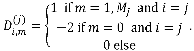
- Alternatively, the penalty term P(f(xi )) may be formed as

- This is a penalty term that penalizes small-scale features and large gradients in the baseline estimate. It should be noted that, as xi,m and f(xi ) are both discrete, the differentiation can be carried out by convolution with a derivative array ∂ j . The operator ∂ j represents a discrete first-order derivative or gradient operator in the dimension j.
- As the penalty term is a scalar quantity, the units of the regularization length scale γj and the squared derivative operator need to cancel each other. As the nth derivative


- The regularization length scale separates image features into features that belong to the out-of-focus contribution from features that belong to the in-focus contribution. Image features having a length scale larger than the length scale reflected in the regularization length scale will be reflected in the baseline estimate. Image features that have a length scale that is smaller than the length scale are not reflected in the baseline estimate. Thus, by setting the regularization length scale to an image feature length scale fl, that e.g. may be predetermined or set by a user, e.g. γj = fl 2 for a first-order derivative of the baseline estimate in the penalty term or γj = fl 4 for a second-order derivative of the baseline estimate in the penalty term, structures of a certain size may be chosen to be reflected in the baseline estimate. In more general terms, the regularization length scale is a function of the image feature length scale, γj = γj (flj ), with the feature length preferably being the sole variable.
- If, for a single input image, two different baselines fI (xi ) and fII (xi ) are computed, where, for one baseline estimate, fI (x i), a first image feature length scale flI , and for the other baseline estimate, fII (xi ), a second image feature length scale flII was used in the respective regularization length scale with flI > flII, then fII (xi ) - fI (xi ) yields those structures in the image of which the length scales are between flI and flII.
- Instead of or in addition to a derivative or a linear combination of derivatives of the baseline estimate, the penalty term may contain a feature-extracting, in particular linear, filter or a linear combination of such filters. Feature-extracting filters may be a Sobel-filter, a Laplace-filter, and/or a FIR filter, e.g. a high-pass or band-pass spatial filter having a pass-band for high spatial frequencies.
- It should be noted in this context, that in a two-dimensional input image, such as a color image, multispectral image or hyperspectral image, which has a plurality of different color channels, the wavelength or color may form a third dimension, if the color channels are not regarded separately. A separate image feature length scale which reflects a spectral length scale is then assigned to this dimension. Such an image feature length scale may be used to assign abrupt color changes to the "in-focus" component and long-range color changes to the "out-of-focus" component.
- Moreover, in a three-dimensional color, multispectral and hyperspectral image, another dimension may relate to the third spatial dimension, for which another image feature length scale may be defined.
- In such a general formulation, the penalty term for the j-th dimension may contain general operators ζ (j) and be expressed as

- The least-square minimization criterion M(f(xi )) may be minimized using known methods. In one instance, a preferably iterative minimization scheme may be used. In particular a half-quadratic minimization scheme may be used. For performing the minimization, the baseline estimator engine may comprise a minimization engine, which in particular may be a half-quadratic minimization engine. The minimization scheme or engine may comprise an iteration mechanism having two iteration stages.
- The minimization scheme may e.g. comprise at least part of the LEGEND algorithm, which is computationally efficient. The LEGEND algorithm is described in Idier, J. (2401): Convex Half-Quadratic Criteria and Interacting Variables for Image Restoration, IEEE Transactions on Image Processing, 10(7), p. 1001-1009, and in Mazet, V., Carteret, C., Bire, D, Idier, J., and Humbert, B. (2405): Background Removal from Spectra by Designing and Minimizing a Non-Quadratic Cost Function, Chemometrics and Intelligent Laboratory Systems, 76, p. 151-163. Both articles are herewith incorporated by reference in their entirety.
- Other minimization schemes which may be applied for computing the baseline estimate are described in Wang, G. et al. (2014): Morphological Background Detection and Illumination Normalization of Text Image with Poor Lighting, PLoS One, 2019, 9 (II), e110991, which is incorporated by reference in its entirety.
- The LEGEND algorithm introduces discrete auxiliary data d(xi ) that are preferably of the same dimensionality as the input image data. The auxiliary data are updated at each iteration depending on the latest initial baseline estimate, the truncated quadratic term and the input image data.
- In the LEGEND algorithm, the least-square minimization criterion is minimized using two iterative steps until a convergence criterion is met.
- A suitable convergence criterion may, for example, be that the sum of the differences between the current baseline estimate and the previous baseline estimate across all locations xi is smaller than a predetermined threshold.
- In a further improvement, the convergence criterion may be expressed as

- As a starting step in the LEGEND algorithm, an initial set of baseline estimation data for the baseline estimate is defined.
- The LEGEND algorithm may be started by selecting a starting set of coefficients ak for a first baseline estimate

- If a spline fit is used, the initial condition for starting the LEGEND algorithm may be d(xi ) = 0, f(xi ) = I(xi ) and the iteration is started by entering at the second iterative step.
- In the first iterative step, the auxiliary data may be updated as follows:

- In a second iterative step, the baseline estimate f (l)(xi ) are updated based on the previously calculated auxiliary data d (l)(xi ), the baseline estimate f (l-1)(xi ) from the previous iteration (l - 1) and on the penalty term P(xi ).
- The baseline estimate f (l)(xi ) may be minimizing a minimization criterion M(f(xi )) which has been modified for the LEGEND algorithm by including the auxiliary data.
- In particular, the updated baseline estimate may be computed using the following formula in the second iterative LEGEND step:

- The second iterative step may update the baseline estimate using the following matrix computation:


- The two iteration steps for updating d (l)(xi ) and f (l)(xi ) are repeated until the convergence criterion is met.
- According to a highly preferable aspect, the second step of the LEGEND algorithm is modified using a convolution instead of a matrix computation. This greatly reduces the computational effort.
- More particularly, it is preferred that the updated baseline estimate f (l)(xi ) is computed directly by convolving a Green's function with the sum of the input image data and the updated auxiliary data.
- According to a more concrete aspect of the inventive solution, the second iterative step of the LEGEND algorithm may be replaced by the following iterative step, where the updated baseline estimate f (l)(xi ) is computed in the l-th iteration using a Green's function G(xi ) as follows

- This step reduces the computational burden significantly as compared to the traditional LEGEND algorithm.
- The reduced computational burden results from the fact that according to the inventive second iterative step, a convolution is computed. This computation can be efficiently carried out using an FFT algorithm. Moreover, the second iterative step may make full use of an array processor, such as a graphics processing unit or an FPGA due to the FFT algorithm. The computational problem is reduced from (Mx × My )2 to Mx × My if the input image data and all other arrays are two-dimensional. For a general N-dimensional case, the computational burden is reduced from (M 1×···×MN )2 dimensional matrix calculations to the computation of a FFT with (M 1×··· ×MN ) -dimensional arrays
- Thus, the computation and removal of the baseline estimate may be carried out very quickly, preferably in real time for two-dimensional input image data. A (2k × 2k) output image may be computed in 50 ms and less.
- In one specific embodiment, the Green's function may have the form


- In general, the discrete penalty array


- A big advantage of the above Green's function is that any form of penalty term P(f(xi )) may benefit from the fast computation of the second iterative step in the minimization engine. Thus, in the embodiment which uses the Green's function, any penalty term for obtaining a good baseline estimate may be used.
- For the general formulation of the penalty term


- For example, if the penalty term is


- With any variant of the above-described computational schemes, the image processing apparatus may be configured to compute at least one baseline estimate f(xi ), for an input image I(xi ). However, a common baseline estimate f(xi ) may be used for two or more input images, if these input images differ by less than a predetermined amount. For example, a correlation of the two or more input images may be computed and, if the correlation is above a predefined threshold, the same baseline estimate is used. This decreases the computational burden.
- The set of input images that is retrieved by the image processing apparatus may represent a stack of input images that were recorded e.g. by a microscope or an endoscope, at different focus distances of an objective, such as an autofocus objective. The set may comprise N input images I 1(xi )...IN (xi ). Alternatively or additionally, the set of input images may represent a stack of input images that were recorded e.g. by a microscope or an endoscope at different positions in a plane perpendicular to an optical axis of an optical system, in particular of an objective of the optical system, especially an autofocus objective, or to the focus distance or, equivalently, parallel to the focus plane, i.e. that are shifted in the x-/y-direction, i.e. in a direction parallel to the focal plane or, equivalently, perpendicular to the focus distance. Such an auto-focus system may be used to track objects that move. The set of input images, or subsequent sets of input images may represent a time-varying object, different input images of a time-invariant object, such as input images taken with different focal lengths, from different positions, and/or in different colors, or any combination thereof.
- The image processing apparatus may be configured to remove the at least one baseline estimate f(xi ) from the respective input image of the set, for which the baseline estimate has been computed. If this step is repeated for each of the input images of the set, a set of output images is obtained. As a result, an output image is obtained for each input image. Thus, from N input images N output images O 1(xi )...ON (xi ) are obtained.
- The set of output images is de-blurred when the out-of-focus component is removed, e.g. by subtraction, as described above. The de-blurred output images allow a more reliable determination of the output image that is in focus, i.e. the focused output image OAF (xi ).
- By adjusting the image feature length scale fl, the focused output image may be determined using only features that have a certain length scale. If the determination of the focused output image is to be based on features that have a length scale which is larger than the image feature length scale fl, the baseline estimate may be directly used as the output image. If the determination of the focused output image is to be based on features that have a length scale which is smaller than the image feature length scale, the selection is based on an output image which is computed by removing the baseline estimate from the respective input image. If the selection of the focused output image is to be based on features that have a length scale which is within a certain range, two baseline estimates fI (xi ) based on a first length scale fl I,j and fII (xi ) based on a different second image feature length scale flII,j may be computed and subtracted for each input image to obtain a respective output image. The image feature length scales may be independent of the direction j.
- The focused output image may be determined from the set of output images by using a focus function. Focus functions are e.g. described in Groen, F.C.; Young, I.T.; Ligthart G. (1985): A Comparison of Different Focus Functions for Use in Autofocus Algorithms, in: Cytometry 1985, 6(2): 81-91, which is herewith incorporated by reference in its entirety.
- In particular, the focus function may comprise at least one focus function of the following list:
- Computation of an amount of entropy, for example information entropy, contained in the input image and/or the output image;
- Computation of a contrast in at least part of the input image and/or the output image;
- Computation of an intensity and/or intensity distribution in at least part of the input image and/or the output image;
- Computation of a phase correlation;
- Computation of a correlation with a predetermined pattern.
- As can be seen from the above, the term "focus" is to be understood broadly as not only comprising the identification of the output image that is sharpest but also as the identification of the output image that contains a certain pattern and/or the sharpest and/or brightest and/or best correlating representation of a pattern, such as for object tracking.
- For example, that output image may be selected as a focused output image OAF (xi ) that has the lowest information entropy.
- For pattern correlation, a static or variable pattern may be used. For example, the pattern may be predetermined by a user. Alternatively, a previously-selected focused output image may be used as a pattern, automatically or set by the user.
- Any output image of the set of output images may be post-processed before selecting the focused output image from the set. The post-processing may comprise at least one of deconvolution, histogram modification, unsharp masking, edge enhancement, noise reduction, and/or image morphology techniques to enhance the sharpness of images, such as top-hat transformations.
- Likewise, the input images may be pre-processed before computing the baseline estimate. For example, a top-hat transform may be carried out on one or more, or all input images. Further, the pre-processing of an input image may comprise at least one of deconvolution, histogram modification, unsharp masking, edge enhancement, noise reduction, and processing to increase sharpness. The pre-processing serves to optimize the image quality. The pre-processing may further comprise filtering at least parts of an input image e.g. using image analysis workflows and/or machine learning.
- The image processing apparatus may further be configured to control an autofocus objective depending on the focused output image, such as depending on the location of the focused output image in the set of output images, or on a focus distance, in which the input image, which resulted in the output image that was selected as the focused output image, was recorded. For example, the input image and/or the output image may comprise depth data which are representative of the focus distance of a focal plane, in which the respective input image was recorded. The image apparatus may be configured to control the autofocus objective depending on the depth data.
- For example, the image processing apparatus may be configured to control an imaging system to record a set of input images centered around the focal plane of the input image that resulted in the focused output image, e.g. by a (motorized) xy-movement of a specimen holder or a specimen table of the imaging system.
- For object tracking, the image processing apparatus may be configured to control movement of the field of view relative to a probe volume or probe depending on the focused output image. In such an embodiment, the input image and/or the output image derived from the input image, may contain positional information representing a position parallel to the focal plane, preferably in addition to depth data as described above.
- For example, the image processing apparatus may be configured to move the field of view and the probe volume relative to each other depending on the focused output image. In doing so, an object may be tracked and be kept in a predetermined position, e.g. the center, of the field of view.
- The image processing apparatus may further comprise an image processor, which may be configured to compute the baseline estimate. The image processor may comprise a baseline estimator engine. The baseline estimator engine may be adapted to compute a baseline estimate and to obtain an output image from the baseline estimate. The baseline estimator engine may comprise a discrete representation of least-square minimization criterion (M(xi )).
- The image processor, the baseline estimator engine and the minimization engine may each be implemented in hardware, in software or as a combination or hardware and software. For example, at least one of the image processor, the baseline estimator engine, and the minimization engine may be at least partly be implemented by a subroutine, a section of a general-purpose processor, such as a CPU, and/or a dedicated processor such as a CPU, GPU, FPGA, vector processor and/or ASIC.
- The apparatus may comprise an image storage section. More specifically, the image processor may comprise the image storage section. The signal storage section may be configured to contain the input image data, at least temporarily. The signal storage section may be implemented purely in hardware or in software, or as a combination of hardware and software. For example, the storage section may be an array of data or a subroutine. Alternatively or additionally, the storage section may comprise a hard disk, a memory device and comprise volatile and non-volatile memory, in which the array and/or subroutine is stored.
- The apparatus may comprise an input section. More specifically, the image processor may comprise the input section. The input section may be adapted to retrieve the input image. The input section may be implemented purely in hardware or in software, or as a combination of hardware and software. For example, the input section may be a software function, e.g. a data transfer protocol, and comprise an array of data which serves as an interface for data transfer. Alternatively or additionally, the input section may comprise at least one standardized connector such as a USB, HDMI and/or DisplayPort connector.
- The apparatus may comprise an output section. More specifically, the image processor may comprise the output section. The output section may be adapted to output the output image. The output section may be implemented purely in hardware or in software, or as a combination of hardware and software. For example, the output section may be a software function, e.g. a data transfer protocol, and comprise an array of data which serves as an interface for data transfer. Alternatively or additionally, the output section may comprise at least one standardized connector such as a USB, HDMI and/or DisplayPort connector.
- The image processing apparatus may be part of a microscope or endoscope, which preferably comprises an autofocus objective. The autofocus objective is preferably configured to be controlled by the image processing apparatus depending on the focused output image.
- The observation device may comprise an actuating system for moving a probe relative to a field of view of an objective. The image processing apparatus may be configured to control the position of the field of view relative to the probe by operating the actuator system. For example, a set of subsequent input images may be recorded centered around the location, here in the x-, y- and possibly also the z-direction of the previous focused output image.
- Another way of implementing the baseline estimation and autofocus algorithm is to train a machine learning device such as an artificial neural network, e. g. a convolutional neural network, using pairs of input image data and output image data, where the output image data have been generated using an embodiment of the above described method. A machine learning device which has been trained this way, or, equivalently, a copy of such a trained device can be regarded as an implementation of the method which has been used to generate the training pairs of input and output image data.
- It is to be noted that the apparatus and method provide best results if the input image I(xi ) are - in the case of input image data as input image data - not convolved or deconvolved before the removal of the out-of-focus or in-focus component. Any deconvolution provides the best results if the image to be deconvolved is preprocessed by having the baseline estimate removed or corresponding to the baseline estimate.
- Next, the image processing apparatus, the image processing method and the observation device are further described by way of example only using a sample embodiment, which is also shown in the drawings. In the drawings, the same reference numerals are used for features which correspond to each other with respect to at least one of function and design.
- The combination of features shown in the enclosed embodiment is for explanatory purposes only and can be modified. For example, a feature of the embodiment having a technical effect that is not needed for a specific application may be omitted. Likewise, a feature which is not shown to be part of the embodiment may be added if the technical effect associated with this feature is needed for a particular application.
- In the following examples, the input image data and the output image data are input image data and output image data respectively for the purpose of explaining the advantages of the invention. As is clear from above, any other type of image data may be used instead of or in addition to image data without any changes to the baseline estimate.
- Fig. 1
- shows a schematic representation of an embodiment of an image processing apparatus for use in an autofocus system, an autofocus system and an observation device comprising and autofocus system;
- Fig. 2
- shows a schematic representation of input image data, an in-focus contribution in the input image data, an out-of-focus contribution in the input image data, baseline estimation data and output image data.
- Fig. 3
- shows a schematic rendition of a flow chart for an embodiment of an autofocus based on a baseline estimation;
- Fig. 4
- shows detail IV of
Fig. 3 ; - Fig. 5
- shows a schematic rendition of a set of input images; and
- Fig. 6
- shows a schematic rendition of a set of output images.
- First, the structure and function of an image processing apparatus 1 and method is explained with reference to
Fig. 1 . The image processing apparatus 1 may be part of anobservation device 2, such as an endoscope (not shown) or a microscope 2a. Just for the purpose of explanation, a microscope 2a is shown as an example of anobservation device 2. For the purpose of the apparatus and method, there is no difference between endoscopes of microscopes. - The
observation device 2 may comprise animaging system 4, which is adapted to captureinput image data 6, e.g. with one ormore cameras 8, preferably in digital format. The camera may comprise animage sensor 9. The image sensor may comprise a photon detector, a photo diode, a line sensor, a sensor array, a monochrome, a CCD, an RGB, a multispectral or a hyperspectral line or array sensor which records theinput image data 6 in one ormore color channels 10, wherein eachchannel 10 preferably represents a different light spectrum range of electromagnetic radiation. Theinput image data 6 are also designated as input image I(xi ) in the following. - In particular, the
imaging system 4 or, more specifically, itscamera 8 may be configured to capture a stack or set 11, or subsequent stacks or sets 11, of input images I(xi ). Theset 11 contains N input images I 1(xi )...IN (xi ). Thus, at least some of the input images of a set are captured at different focus distances 12. - For automatically finding a focus or holding a focus, the
imaging system 4 may comprise anautofocus system 13. Theautofocus system 13 is preferably a passive autofocus system, i.e. it has no active sensor for measuring thefocus distance 12, but may also be an active autofocus system. Further, theautofocus system 13 is preferably software-based. The image processing apparatus 1 may be a part of theautofocus system 13. The observation device and/or the autofocus system may comprise anautofocus objective 14. - In the case of a CCD camera recording in RGB color space, for example, three
channels 10, e.g. a R-channel, a G-channel and a B-channel, may be provided to represent a visible-light, or white-light, color input image of anobject 15. In the case of a multi- or hyperspectral camera, more than threechannels 10 may be used per input image in at least one of the visible light range, the IR light range, the NIR light range and the ultraviolet light range. - The
input image data 6 may be considered as being two-dimensional if asingle channel 10 is contained in a two-dimensional image. The input image may have a higher dimensionality than two if more than twochannels 10 are considered as constituting the input image I(xi) and/or if theinput image data 6 represent a three-dimensional array, such as a three-dimensional image. - The
object 15 is located in aprobe volume 16 of theimaging system 4. The probe volume is configured to receive theobject 15 to be inspected by the apparatus 1. For this, the probe volume should be located in a field ofview 17 of theimaging system 4, in particular of the objective 14. - The observation apparatus may comprise an
actuator system 18, which is configured to move the field ofview 17 and theprobe volume 16 or theobject 15 relative to each other and/or relative to the autofocus objective. The actuator system may comprise e.g. an electric motor to move the object and/or part of the imaging system, such as the objective 14 in a direction perpendicular to the focus distance or parallel to a focal plane. This movement may occur simultaneously or synchronized with a change of thefocus distance 12. - The
object 15 may comprise animate and/or inanimate matter. Theobject 15 may further comprise one or more fluorescent materials, such as at least onefluorophore 20. A multispectral or hyperspectral camera may have achannel 10 for each different fluorescence spectrum of the fluorescent materials in theobject 15. For example, each fluorophore 20 may be represented by at least onechannel 10 which is matched to the fluorescence spectrum triggered by anillumination system 19. - Alternatively or additionally,
separate channels 10 may be provided for auto-fluorescence spectra or for spectra of secondary fluorescence, which is triggered by fluorescence excited by theillumination system 19, or for lifetime fluorescence data. Of course, theillumination system 19 may also or solely emit white light or any other composition of light without triggering fluorescence in theobject 15. Themicroscope 2 may be adapted to excite fluorescence e.g. offluorophores 20 within anobject 15 with light having a suitable fluorescence excitation wavelength by theillumination system 19. Theillumination system 19 may be arranged opposite theimaging system 4 with respect to theprobe volume 16 and/or on the same side as theimaging system 4. - If the
illumination system 19 is arranged on the same side as theimaging system 4, its light may be guided through theautofocus objective 14, through which also theinput image data 6 are acquired. Theillumination system 19 may comprise or consist of one or more flexible light guides to direct light onto theobject 15 from one or more different directions. A suitable blocking filter (not shown) may be arranged in the light path in front of thecamera 8 or theautofocus objective 14, e.g to suppress glare. In case of fluorescence, a blocking filter preferably blocks only the illumination wavelength and allows the fluorescent light of the at least onefluorophore 20 in theobject 15 to pass to thecamera 8. - If the illumination system is arranged opposite the
probe volume 16, its light may pass through theprobe volume 16. - It is apparent - without limitation to the general - that the
input image data 6 can be captured by any kind of microscope, in particular with a fluorescence light microscope operable in a wide-field mode and/or using a confocal laser scanning microscope, or by any kind of endoscope. - The
set 11 of input images may be captured by e.g. using light-field technology, z-stacking in microscopes, images obtained by a SPIM microscope, a SCAPE microscope, moving the field of view and the probe or probe volume relative to each other or relative to the objective 14 in a direction perpendicular to the focus distance and/or parallel to a focal plane, and/or a three-dimensional reconstruction of images obtained by a SPIM microscope. Each input image of theset 11 represents adifferent focus plane 22. In the case of a three-dimensional image, eachfocus plane 22 may be considered as a two-dimensional grey value orcolor input image 6. Each plane may compriseseveral channels 10. Theautofocus system 13 is preferably configured to capture an input image I(xi ) automatically in a predetermined focal plane. For the sake of simplicity, the index of the input image in theset 11 is omitted in the following. - The
input image data 6 are a digital representation of a quantity I(xi ), such as an intensity, where xi represents a location in theinput image data 6 and I is the quantity at that location which constitutes the input image. The term xi is a shortcut notation for a tuple {x 1 ; ···;xN } containing N dimensions and representing a discrete location xi in the discrete input image data. A location xi may be a pixel or a preferably coherent set of pixels in the input image data. The discrete location xi denotes e.g. a pair of discrete location variables {x 1 ; x 2} in the case of two-dimensional input image data and a triplet of discrete location variables {x 1 ; x 2 ; x 3} in the case of three-dimensional input image data. In the i-th dimension, the array may contain Mi locations, i.e. xi = {x i,1 ,...,xi,Mi }. In total, I(xi ) may contain (M 1 × ··· × MN ) elements. I(xi ) may be an array of discrete real-valued, e.g. represented as digital floating-point numbers, or of integer-valued data. - The image processing apparatus 1 may further comprise a
storage section 24 which is adapted to contain, at least temporarily, theinput image data 6. Thestorage section 24 may comprise a volatile or non-volatile memory, such as a cache memory of aCPU 25 of an e.g. general-purpose computing device 26, such as a PC, and/or of a GPU 27. Thestorage section 24 may further comprise RAM, a hard disk drive or an exchangeable storage section, such as a USB stick or an SD card. Thestorage section 24 may comprise any combination of these types of memory. Alternatively or additionally, the storage section may also be implemented as a software device, e.g. as a subroutine, function or an array. - For retrieving the
set 11 of input images, aninput section 28 may be provided. Theinput section 28 may comprise standardized connection means 30, such as standardized data exchange protocols, hardware connectors and/or wireless connections, or any combination thereof. Examples of standardized connectors which may be connected to thecamera 8 are HDMI, USB and RJ45 connectors. Alternatively or additionally, the input section may be implemented in software, e.g. as a subroutine, function or array, which serves as a software interface for the transfer of data. Theinput section 28 may be part of the image processing apparatus 1. - The image processing apparatus 1 may be configured to compute for each input image I(xi ) in the set 11 an output image O(xi ), so that a stack or set 31 of output images is obtained from the set of input images. Thus, for N input images I 1(xi )...IN (xi ), N output images O 1(xi )...ON (xi ) are computed. Again, the indices are omitted for the output images in the following to keep the notation simple.
- The image processing apparatus 1 may further comprise an
output section 32 which may comprise standardized connection means 34, such as standardized data exchange protocols, hardware connectors and/or wireless connections, each configured to outputoutput image data 35 to one or more displays 37. Theoutput image data 35 have preferably the same dimensionality as theinput image data 6, and are represented by a discrete array of discrete values, forming an output image O(xi ). Theoutput image data 35 may be real or integer-valued. Alternatively or additionally, the output section may be implemented in software, e.g. as a subroutine, function or array, which serves as a software interface for the transfer of data. Theoutput section 32 may be part of the image processing apparatus 1. - For computing an output image O(xi ) from an input image I(xi ), an
image processor 38 may be provided. Theimage processor 38 may be at least partly hardware, at least partly software and/or a combination of both hardware and software. For example, theimage processor 38 may comprise at least one of aCPU 25 and a GPU 27 of a general-purpose computing device 26, as well as data structures and sections that have been coded in software and temporarily exist as structural entities in theCPU 25 and/or the GPU 27 in an operational state. Theimage processor 38 may also comprise additional hardware such as memory and/or one or more ASICs which have been specifically designed in carrying out operations required for the image processing apparatus and method. - Before continuing the further description of
Fig. 1 , the general principle of processing an input image I(xi ) of aset 11 is explained with reference toFig. 2 . For estimating the baseline f(xi ) of an input image I(xi ), theimage processor 38 may comprise abaseline estimator engine 40. The following holds for any of the input images in theset 11. - The input image I(xi ) may be assumed to be composed additively from an in-focus component III (xi ), which contains the in-focus component, i.e. structures of the
object 15 that lie within thefocus plane 22 of the input image, and an out-of-focus component II (xi ), which may mainly contain light from the background, i.e. light from outside thefocus plane 22. Neither II (xi ) nor III (xi ) are known and therefore have to be estimated. - For estimating II (xi ) and III (xi ), it is assumed that the out-of-focus component III (xi ) is smooth and consists of or comprises predominantly components having low spatial frequency, i.e. large spatial extent. The out-of-focus component thus represents a baseline about which the in-focus component I 1(xi ) fluctuates at a higher spatial frequency. The out-of-focus component III (xi ) is assumed to be smooth and as having large length scales; the in-focus component II (xi ) is, by contrast, assumed not to be smooth and to contain at least one of peaks and valleys. Depending on the application, the information of interest may reside either in I 1(xi ) or in III (xi )
- An estimate for the out-of-focus component III (xi ) is represented by a baseline estimate f(xi ). The baseline estimate is a discrete array of baseline estimation data 44 that has preferably the same dimensionality as the input image. The baseline estimate f(xi ) may be at least temporarily present in the
storage section 24. As at least one baseline estimate f(xi ) is computed for each input image, theset 11 of input images results in a set 45 of baseline estimates. If it is determined, e.g. by computing a correlation, that two input images I(xi ) do not deviate from one another beyond a predetermined threshold, a baseline estimate f(xi ) which has already been computed for one of the two input images I(xi ) may be used for the other of the two input images I(xi ). For this, each baseline estimate f(xi ) may be stored at least temporarily in the storage section. In the set 45, each baseline estimate is associated with one input image of theset 11. - Once the baseline estimate has been computed, the in-focus component, here represented as O(xi ) may be obtained by removing, in particular, subtracting the baseline estimate f(xi ) from the input image I(xi ) at each location xi .
- The image processing apparatus 1 may be configured to preprocess at least one input image, preferably all input images, I(xi ) of a
set 11. For example, the image apparatus 1 may be configured to apply a top-hat transform to the at least one input image I(xi ). In addition or alternatively, the image processing apparatus 1 may be configured to apply in the pre processing a filter, unsharp masking, histogram equalization, morphological filtering, and other methods for enhancing the image quality. - The
baseline estimator engine 40 is configured to compute the baseline estimate f(xi ) by a fit to at least a subset of theinput image data 6 which make up an input image I(xi ). Preferably, the fit to at least the subset of the input image data is a spline fit. - For a computationally efficient spline fit, the
baseline estimator engine 40 may comprise a minimization engine 46, which may, for example, be a subroutine or a combination of a hardwired algorithm and a matching software. The minimization engine 46 may be configured to execute a minimization scheme and, towards this end, may comprise twoiteration stages - Preferably, the minimization engine 46 comprises a convolution to compute the baseline estimate f(xi ) in the
second iteration stage 50. As the convolution can be computed more efficiently on an array processor using a FFT, it is preferred that theimage processor 38 includes an array processor such as a GPU 27. In operation, the image processor comprises the minimization engine 46. - With reference to
Fig. 3 , the steps of computing an output image O(xi ) from an input image I(xi ) are described as they are performed by the image processing apparatus 1. - In a
first step 60, various parameters of thebaseline estimator engine 40, which need to be preset, may be defined by a user, e.g. using a graphical user interface 62 (Fig. 1 ). The parameters may comprise the type of fit to theinput image data 6 that is to be performed by thebaseline estimator engine 40. For example, a user may choose between a polynomial fit and a spline fit of the baseline estimation data 44 to theinput image data 6. - Further, the user may choose between a variety of penalty terms P(f(xi )) which are used in the minimization scheme. The penalty term determines the shape of the baseline estimate by penalizing the representation of components of the in-focus contribution II (xi ) in the baseline estimate.
- For example, the user may be presented with a selection of various penalty terms that penalize non-smooth characteristics of the baseline estimate. For instance, the penalty term may be a high-pass spatial frequency filter for the baseline estimation data 44, which gets larger if the baseline estimate contains components having high spatial frequency. Other penalty terms may include a gradient of the baseline estimate. Another example of a penalty term may be the curvature of the baseline estimate. Further, feature extracting filters, such as a Sobel, Laplace and/or FIR band-pass, high-pass or low-pass filter may be selected by the user as penalty term. Further, a linear combination of any of the above may be selected. Different penalty terms may be selected for different dimensions or for different channels of the
input image data 6. - The general representation of the penalty term is as follows

- In the following, it is assumed that the user selects a gradient-based roughness penalty term based on the gradient of the baseline estimate f(xi,m ) having the following form

- This penalty term penalizes large gradients in the baseline estimate. The operator ∂ j represents a first-order derivative or gradient in the dimension j. However, the user may be presented with a selection and select any order and combination of derivatives of the baseline estimate. For example, the user may select a second-order derivative


- Using the above gradient-based penalty term, the parameters to be specified by the user further comprise an array γj of direction-dependent regularization length scales for each direction or dimension j. The direction-dependent regularization length scale γj represents a direction-dependent length scale such as an image feature length scale flj. A feature in the image that has a length scale in direction xj that is smaller than the corresponding image feature length scale flj is considered to belong to the in-focus contribution and not to the baseline. Structures in the input image having a length larger than the image feature length scale in the respective direction j are considered to belong to the baseline. As is clear from the index j of γj , the regularization length scale and thus the image feature length scale may be different in each direction. Of course, there may also be used just one constant image feature length scale and/or one constant regularization length scale for any direction. The user may be prompted to input either the regularization length scale or the image feature length scale. The latter is preferred as it is more intuitive for the user and independent of the exact formulation of the penalty term.
- As the penalty term P(f(xi )) is a scalar value, the product of the regularization length scale, γj , and the general operator ζ (i)(f(x i,m)) must be scalar. If the general operator is for example a gradient, the regularization length scale has the unit [length]2. If the general operator is a second-order derivative, the regularization length scale has the unit [length]4. In this embodiment where a gradient is used, the regularization length scale has the unit [length]2and is thus equal to the square of the image feature length scale

- The user may further select whether he wants to have image features that have a length scale larger than the specified image feature length scale or smaller than the specified image feature length scale regarded as the content of interest. In the former case, the baseline estimate itself will be regarded as output image, O(xi ) = f(xi ), in the latter case, the baseline estimate needs to be removed from the input image to obtain the desired content.
- Further, the user may select a first and a second image feature length scale, flI,j and flII,j, flI,j ≠ flII,j, or corresponding regularization length scale γI,j and γII,j, which may also be direction-independent and in this case be formulated as γI and γII, or flI and flII, respectively. For each of the first and the second image feature length scale, a different baseline estimate fI (xi ) and fII (xi ) may be computed from the resulting, different, penalty term. In the baseline estimate fI (xi ), image features having a length scale larger than the feature image length scale flI are contained whereas in the baseline estimate fII (xi ) image features having a length scale larger than the feature length scale flII are contained. Image feature having a length scale smaller than the first and the second image feature length scale are not represented in the respective baseline estimate or at least strongly suppressed.
- Specifying two different image feature length scales allows to compute an output image O(xi ) in which only features of a length scale are represented that falls within the range limited by the two image feature length scales simply by removing, in particular subtracting, one baseline estimate fI (xi ) from the other, fII (xi ).
- Further, the user may specify a pattern Q(xi ) for which to search in the set 31 of output images. The pattern may e.g. be an image of an
object 15 or a part thereof. For example, the pattern may be a mitochondrion. - Further, the user may choose between a symmetric and asymmetric, in particular truncated, quadratic term ϕ(ε(xi )), which also determines the shape of the baseline estimate by specifying the effect of large peaks on the baseline estimate. A value for the truncation may also be specified by the user.
- For example, the user may select the following asymmetric, truncated quadratic:

- Finally, the user may select a convergence criterion and/or a threshold value t which has to be reached by the convergence criterion.
- After the user-definable parameters for the
baseline estimator engine 40 have been set, the data are initialized instep 64 for theiterative minimization scheme 66. -
Fig. 4 , detail IV ofFig. 3 is shown to explain theminimization scheme 66 in closer detail. Theminimization scheme 66 comprises thefirst iteration stage 48 and thesecond iteration stage 50. - In principle, the
minimization scheme 66 as carried out by the minimization engine 46 may be the LEGEND algorithm. However, it is preferred to modify the second step of the LEGEND algorithm may be modified to significantly reduce the computational burden. - In the shown embodiment, the second
iterative stage 50 is entered after initializing the data atstep 64. At this point, the first estimate f (1)(xi ) of the baseline estimate is computed by using a convolution of the input image data with a Green's function G(xi ). The index in parenthesis indicates the iteration index.
- For the gradient-based penalty term used in this embodiment, the Green's function is defined as follows:


- Then, in the
first iteration stage 48, an updated version of auxiliary data d (l)(xi ) may be computed using the current baseline estimate f (l-1)(xi ) as follows:
- The parameter α is a constant which may have been specified by the user.
- Next, in the second
iterative stage 50, the updated baseline estimate f (l-1)(xi ) is computed using the updated auxiliary data d (l)(xi ) of the current iteration (l) as follows
- In the next step, it is checked whether the
convergence criterion 68 is met. If this is not the case, theminimization scheme 66 proceeds toiterative step 48 using the updated baseline estimate f (l)(xi ). - The
iterative minimization scheme 66 is carried out by the minimization engine 46 until aconvergence criterion 68 is met. In the embodiment, the following convergence criterion is used as an example:
convergence criterion 68 is met, it is assumed that the baseline estimate been successfully computed. - Instead of the above minimization scheme for the baseline estimation, any other minimization scheme may be used, e.g. a minimization scheme described in Wag, G. et al. (2014): Morphological Background Detection and Illumination Normalization of Text Image with Poor Lighting, PLoS One, 2019, 9 (II), e110991.
- If two different image feature length scales flI,j and flII,j have been specified by the user, the
above steps 64 to 68 are carried out twice, once for each different image feature length scale, resulting in two baseline estimates fI (xi ) and fII (xi ), one baseline estimate for each different image feature length scale. In other words, one baseline estimate fI (xi ) is computed using the regularization length scale

- In
step 70, the output image O(xi ) is obtained from the respective input image. How the output image is computed depends on the user settings. - If, for example, the user has selected that the features of the image he is interested in have a length scale smaller than the selected image feature length scale fl, the baseline estimate f(xi ) is removed, in particular subtracted, O(xi ) = I(xi ) - f(xi ), from the input image data I(xi ) to obtain the output image data O(xi ) in
step 70. - If the user has selected that he is interested in the features that are larger than the image feature length scale, the output image is set to be equal to the baseline estimate, O(xi ) = f(xi ) in
step 70. - If the user is interested in features in an input image that have a length scale between the two specified image feature length scales flI and flII, wherein flII > flI , then the baseline estimate based on the larger image feature length scale is subtracted from the baseline estimate based on the smaller image feature length scale, O(xi ) = fI (xi ) - fII (xi ).
-
Step 70 may further contain a post-processing of the output image. The post-processing may comprise any automatic image enhancement such as at least one of unsharp masking, deconvolution, edge enhancement, histogram modification and noise reduction. - The
steps 64 to 70 are carried out for each input image of theset 11, so that for each input image I(xi ) an output image O(xi ) is obtained. -
Step 72 relates to identifying the focused output image OAF (xi ) in theset 36 that defines the result of the autofocusing procedure. For selecting the output image OAF (xi ) several focus functions may be applied independently from another or in any combination, depending of the application and the user settings. - The focused output image OAF (xi ) may e.g. be selected by computing a correlation between the pattern Q(xi ), or perform any other kind of pattern-matching. The output image, in which the pattern-matching results in the highest correlation may be selected. A focus function of this type may in particular be used to identify or track features across subsequently recorded sets 11 of input images.
- The output image of the
set 36 may be selected as focused output image OAF (xi ) that has the highest contrast, either overall or in one or more color channels, and/or in one or more predetermined or automatically determined regions. - The output image of the
set 36 may be selected as focused output image OAF (xi ) that has an information entropy that is below a predetermined, e.g. user-specified, threshold. - The output image of the
set 36 may be selected as focused output image OAF (xi ) that has the highest intensity and/or narrowest intensity distribution overall or in one or more color channels. - Other focus functions are e.g. described in Groen, F.C.; Young, I.T., Ligthart, G.(1985): A Comparison of Different Focus Functions for Use in Autofocus Algorithms, in: Cytometry, 1985 6(2), 81-91, which is herewith interpreted by reference in its entirety.
- The output image of the
set 36 may be selected as focused output image OAF (xi ) that has the highest correlation with the previously selected output image from the previous set of input images. - If there are more than two output images which satisfy the focus function, the output image that lies in the middle may be selected as focused output image OAF (xi ). If two output images satisfy the focus function, the one with the smallerfocus distance may be selected.
- In step 74, the selected output image O(xi ), i.e. OAF (xi ), is stored, e.g. in
storage section 24, and/or displayed, e.g. ondisplay 37. Before being displayed, the selected focused output image OAF (xi ) may be processed further, e.g. undergo deconvolution, unsharp masking or any other image enhancement, that has not yet been performed on the output images O(xi ). - If the
imaging system 4 acquiressubsequent sets 11, e.g. continuously, thesteps 64 to 74 are carried out for each set, preferably in real time. Thus, for each of the input images In (xi ) of theset 11, n = 1 ...N, a baseline estimate fn (xi ) is obtained using preferably the same image feature length scale fl. Each output image On (xi ) is computed as described above from the respective at least one baseline estimate fn (xi ) or fI (xi ), fII (xi ), or the respective input image In (xi ) and its baseline estimate fn (xi ). -
Fig. 5 shows aset 11 of three input images II (xi ), III (xi ), and IIII (xi ) which were obtained by focus stacking using a microscope. The input images are blurred due to a strong out-of-focus component. The blur makes it difficult to determine the correct focused image. -
Fig. 6 shows three output images OI (xi ), OII (xi ), and OIII (xi ), which have been obtained from the respective input image II (xi ), III (xi ), and IIII (xi ) ofFigure 5 by computing a respective baseline estimate fI (xi ), fII (xi ), and fIII (xi ) based on an image feature length scale fl, which was chosen to be the same for all three input images. The baseline estimate fn (xi ), was then removed, in particular subtracted, from the respective input image In (xi ) to obtain the respective output image On (xi ), n = 1,2,3. As can be seen fromFig. 6 , the output images in the set 31 contain significantly less blur, which allows for the determination of a focused image much easier and with greater certainty than by using the original input images. The focused image is determined using a focus function, for example, by selecting the output image of the set 31 which has the highest contrast. In the example ofFig. 6 , output image O 2(xi ) is determined as the focused output image OAF (xi ). - Of course, any number of input images may be contained in the
set 11 to produce the corresponding amount of output images in the set 31. - If two or more input images in a
set 11 or across several input images have only minor differences, the same baseline estimate may be used for each of these input images. This saves computational costs. For example, the image processing apparatus may be configured to store a baseline estimate of an input image, e.g. in the storage device, and to compute a correlation between two different input images and to determine if the correlation exceeds a predetermined threshold. If it is determined by the image processing apparatus that the predetermined threshold is exceeded or not exceeded depending on the correlation measure, the image apparatus may be configured to retrieve the stored baseline estimate of the correlating, previously obtained input image and apply it to compute the output image corresponding to the newly obtained input image. - The image processing apparatus may be configured to control the
actuator system 18 to move the field ofview 17 and theprobe volume 16/object 15 relative to each other and/or theautofocus objective 14 to change thefocus distance 12, depending on the focused output image OAF (xi ) and/or the input image from which the focused output image was derived. For this, each input image or output image may contain positional data, which is representative for a focus distance, a z position and/or a (x,y) position. Thefocus distance 12 and/or the relative position of the field ofview 17 and theobject 15 may be controlled by the image processing apparatus depending on the positional data of the focused output image or the corresponding input image. The image processing apparatus 1 may be configured to generate a focus-distance control signal which is representative of the focus distance to be set by e.g. anautofocus objective 14, depending on the positional data. Alternatively or additionally, the image processing apparatus 1 may be configured to generate an object positioning signal which is representative of the relative position of the field of view and the object to be set by e.g. theactuator system 18. - In particular, the
observation device 2 may be configured to record asubsequent set 11 of input images depending on the focused output image derived from theprevious set 11 of input images. In particular, thesubsequent set 11 of input images may centered about the position of the focused output image of the previous set. - The
observation device 2 may further be configured to move the probe volume relative and the field of view relative to each other depending on the focused output image, the input image from which the focused output image was derived, and/or the positional data in the focused input image or the input image from which the focused output image was derived. - Alternatively or additionally, the
device 2 may be configured to adjust thefocus distance 12 depending on the focused output image, the input image from which the focused output image was derived, and/or the positional data in the focused input image or the input image from which the focused output image was derived. - As used herein the term "and/or" includes any and all combinations of one or more of the associated listed items and may be abbreviated as "/".
- Although some aspects have been described in the context of an apparatus, it is clear that these aspects also represent a description of the corresponding method, where a block or device corresponds to a method step or a feature of a method step. Analogously, aspects described in the context of a method step also represent a description of a corresponding block or item or feature of a corresponding apparatus. Some or all of the method steps may be executed by (or using) a hardware apparatus, like for example, a processor, a microprocessor, a programmable computer or an electronic circuit. In some embodiments, some one or more of the most important method steps may be executed by such an apparatus.
- Depending on certain implementation requirements, embodiments of the image processing apparatus can be implemented fully in hardware orfully in software, or in a combination of both software and hardware. The implementation can be performed using a non-transitory storage medium such as a digital storage medium, for example a floppy disc, a DVD, a Blu-Ray, a CD, a ROM, a PROM, and EPROM, an EEPROM or a FLASH memory, having electronically readable control signals stored thereon, which cooperate (or are capable of cooperating) with a programmable computer system such that the respective method is performed. Therefore, the digital storage medium may be computer readable.
- Some embodiments according to the invention comprise a data carrier having electronically readable control signals, which are capable of cooperating with a programmable computer system, such that one of the methods described herein is performed.
- Generally, embodiments of the present invention can be implemented as a computer program product with a program code, the program code being operative for performing one of the methods when the computer program product runs on a computer. The program code may, for example, be stored on a machine readable carrier.
- Other embodiments comprise the computer program for performing one of the methods described herein, stored on a machine readable carrier.
- In other words, an embodiment of the present invention is, therefore, a computer program having a program code for performing one of the methods described herein, when the computer program runs on a computer.
- A further embodiment of the present invention is, therefore, a storage medium (or a data carrier, or a computer-readable medium) comprising, stored thereon, the computer program for performing one of the methods described herein when it is performed by a processor. The data carrier, the digital storage medium or the recorded medium are typically tangible and/or non-transitionary. A further embodiment of the present invention is an apparatus as described herein comprising a processor and the storage medium.
- A further embodiment of the invention is, therefore, a data stream or a sequence of signals representing the computer program for performing one of the methods described herein. The data stream or the sequence of signals may, for example, be configured to be transferred via a data communication connection, for example, via the internet.
- A further embodiment comprises a processing means, for example, a computer or a programmable logic device, configured to, or adapted to, perform one of the methods described herein.
- A further embodiment comprises a computer having installed thereon the computer program for performing one of the methods described herein.
- A further embodiment according to the invention comprises an apparatus or a system configured to transfer (for example, electronically or optically) a computer program for performing one of the methods described herein to a receiver. The receiver may, for example, be a computer, a mobile device, a memory device or the like. The apparatus or system may, for example, comprise a file server for transferring the computer program to the receiver.
- In some embodiments, a programmable logic device (for example, a field programmable gate array) may be used to perform some or all of the functionalities of the methods described herein. In some embodiments, a field programmable gate array may cooperate with a microprocessor in order to perform one of the methods described herein. Generally, the methods are preferably performed by any hardware apparatus.
-
- 1
- image processing apparatus
- 2
- observation device
- 2a
- microscope
- 4
- imaging system
- 6
- input image data
- 8
- camera
- 9
- image sensor
- 10
- channel
- 11
- set of input images
- 12
- focus distance
- 13
- autofocus system
- 14
- autofocus objective
- 15
- object
- 16
- probe volume
- 17
- field of view
- 18
- actuator system
- 19
- illumination system
- 20
- fluorophore
- 22
- focus plane
- 24
- storage section
- 25
- CPU
- 26
- computing device
- 27
- GPU
- 28
- input section
- 30
- connection means of input section
- 32
- output section
- 34
- connection means of output section
- 35
- output image data
- 36
- set of output images
- 37
- display
- 38
- image processor
- 40
- baseline estimator engine
- 44
- baseline estimation data
- 45
- set of baseline estimates
- 46
- minimization engine
- 48
- first iteration stage
- 50
- second iteration stage
- 60
- setup of baseline estimation parameters
- 62
- graphical user interface
- 64
- initializing of minimization engine and scheme
- 66
- minimization engine and scheme
- 68
- convergence criterion
- 70
- computation of output image data
- 72
- post-processing operation
- 74
- display
Claims (21)
- Image processing apparatus (1) for determining a focused output image (OAF (xi )) in an autofocus system (13), in particular a passive autofocus system (13),
wherein the image processing apparatus (1) is configured- to retrieve a set (11) of input images (I(xi ));- to compute at least one baseline estimate (f(xi )) for at least one [preferably each] input image of the set of input images, the at least one baseline estimate representing image structures having a length scale larger than a predetermined image feature length scale (flj );- to compute a set (31) of output images (O(xi ));- to compute each output image of the set of output images based on one of (a) a different input image of the set of input images and the at least one baseline estimate for this input image and (b) the at least one baseline estimate for a respective different input image; and- to determine one output image of the set of output images as the focused output image. - Image processing apparatus (1) according to claim 1, wherein the image processing apparatus (1) is configured- to remove the at least one baseline estimate (f(xi )) from the respective input image (I(xi )) to obtain an output image (O(xi )) of the set (31) of output images.
- Image processing apparatus (1) according to claim 1 or 2, wherein the image processing apparatus (1) is configured- to compute for an input image (I(xi )) of the set of input images a first baseline estimate (fI (xi )) based on a first predetermined image feature length scale (fl I,j ) and a second baseline estimate (fII (xi )) based on a second image feature length scale (flI,j ), the second image feature length scale being different from the first image feature length scale, and- to compute an output image (O(xi )) based on the first and the second baseline estimate.
- Image processing apparatus (1) according to claim 3, wherein the image processing apparatus is configured- to remove the baseline estimate (fII (xi )) based on a larger image feature length scale (flII ) from the baseline estimate (fI (xi )) based on a smaller image feature length scale (flI ).
- Image processing apparatus (1) according to any one of claims 1 to 4, wherein the image processing apparatus (1) is configured- to obtain a baseline estimate (f(xi )) as an output image (O(xi )) of the set (31) of output images.
- Image processing apparatus (1) according to any one of claims 1 to 5, wherein the image processing apparatus (1) is configured- to compute the baseline estimate (f(xi )) using a least-square minimization criterion for the baseline estimate (M(f(xi ))), the least-square minimization criterion comprising a scalar combination of the image feature length scale and a derivative of the baseline estimate.
- Image processing apparatus (1) according to claim 6, wherein the least-square minimization criterion (M(f(xi ))) comprises a penalty term (P(f(xi ))), the penalty term containing the image feature length scale (flj ).
- Image processing apparatus (1) according to any one of claims 1 to 7, wherein the apparatus (1) is configured to use a focus function to determine the one output image (OAF (xi )) of the set of output images O(xi ) as a focused image.
- Image processing apparatus (1) according to claim 8, wherein the focus function comprises at least one focus function of the following list:- computation of an amount of entropy contained in the input image and/or the output image;- computation of a contrast in at least a part of the input image and/or the output image;- computation of an intensity and/or an intensity distribution in at least part of the input image and/or the output image;- computation of a phase correlation;- computation of a correlation with a predetermined pattern.
- Image processing apparatus (1) according to any one of claims 1 to 9, wherein the apparatus (1) is configured to pre-process at least one input image (I(xi )) of the set (11) of input images (I(xi )) using a top-hat transform.
- Image processing apparatus (1) according to any one of claims 1 to 10, wherein the apparatus (1) is configured to pre-process at least one input image (I(xi )) of the set of input images to improve image quality and/or for filtering.
- Autofocus system (13) comprising an image processing apparatus (1) according to any one of claims 1 to 11, and an imaging system (4) comprising an image sensor (9) and an autofocus objective (14).
- Observation device (2) comprising one of an image processing apparatus (1) according to any one of claims 1 to 11 and an autofocus system according to claim 12, and a display (37), the display being configured to display the focused output image (OAF (xi )).
- Observation device (2) according to claim 13, the observation device being one of a microscope (2a) and an endoscope.
- Image processing method, for determining a focused output image (OAF (xi )) in an autofocus system (13), in particular a passive autofocus system (13), the method comprising the steps of- retrieving a set (11) of input images (I(xi ));- computing at least one baseline estimate (f(xi )) for at least one input image of the set of input images, the at least one baseline estimate representing image structures having a length scale larger than a predetermined image feature length scale (flj );- computing a set (31) of output images (O(xi ));- the step computing the set of output images comprising the step of:
computing each output image of the set of output images based on one of (a) a different input image of the set of input images and the at least one baseline estimate for this input image and (b) the at least one baseline estimate for a respective different input image; and- selecting one output image of the set of output images as the focused output image. - Image processing method according to claim 15, wherein the step of retrieving the set (11) of input images (I(xi )) comprises the step of automatically capturing at least some input images of the set of input images at different focus distances (12) and/or different relative positions of a field of view (12) and an object (15).
- Autofocusing method, comprising the image processing method of claim 15 or 16 and the step of displaying the selected output image (OAF (xi )).
- Computer program with a program code for performing the method according to claim 15 or 16 when the computer program runs on a processor.
- Non-transitory computer readable medium storing a computer program causing a computer to execute the image processing method according to claim 15 or 16.
- Machine learning device for use in an autofocus system, trained by sets of input images and selected output images, wherein the selected output images are created from the set of input images by method according to claim 15 or 16.
- Focused output image (OAF (xi )) being the result of the method according to claim 15 or 16.
Priority Applications (4)
| Application Number | Priority Date | Filing Date | Title |
|---|---|---|---|
| PCT/EP2020/074219 WO2021038103A1 (en) | 2018-03-29 | 2020-08-31 | Image processing apparatus and method for use in an autofocus system |
| US17/637,480 US12106454B2 (en) | 2018-03-29 | 2020-08-31 | Image processing apparatus and method for use in an autofocus system |
| CN202080061266.0A CN114424102B (en) | 2018-03-29 | 2020-08-31 | Image processing apparatus and method for use in an automatic focusing system |
| JP2022513394A JP7589236B2 (en) | 2018-03-29 | 2020-08-31 | Image processing apparatus and method for use in an autofocus system - Patents.com |
Applications Claiming Priority (4)
| Application Number | Priority Date | Filing Date | Title |
|---|---|---|---|
| DE102018204943 | 2018-03-29 | ||
| PCT/EP2018/067244 WO2019185174A1 (en) | 2018-03-29 | 2018-06-27 | Apparatus and method, particularly for microscopes and endoscopes, using baseline estimation and half-quadratic minimization for the deblurring of images |
| PCT/EP2019/058084 WO2019185912A1 (en) | 2018-03-29 | 2019-03-29 | Apparatus and method for baseline estimation in input signal data |
| PCT/EP2019/058089 WO2019185916A1 (en) | 2018-03-29 | 2019-03-29 | Apparatus and method using baseline estimation and half-quadratic minimization for the deblurring of signal data |
Publications (2)
| Publication Number | Publication Date |
|---|---|
| EP3716200A1 true EP3716200A1 (en) | 2020-09-30 |
| EP3716200B1 EP3716200B1 (en) | 2023-10-11 |
Family
ID=62751006
Family Applications (8)
| Application Number | Title | Priority Date | Filing Date |
|---|---|---|---|
| EP18734549.1A Active EP3571663B1 (en) | 2018-03-29 | 2018-06-27 | Apparatus and method, particularly for microscopes and endoscopes, using baseline estimation and half-quadratic minimization for the deblurring of images |
| EP20185781.0A Pending EP3742391A1 (en) | 2018-03-29 | 2018-06-27 | Apparatus and computer-implemented method using baseline estimation and half-quadratic minimization for the deblurring of images |
| EP19712818.4A Pending EP3776453A1 (en) | 2018-03-29 | 2019-03-29 | Apparatus and method using baseline estimation and half-quadratic minimization for the deblurring of signal data |
| EP19712815.0A Active EP3776452B1 (en) | 2018-03-29 | 2019-03-29 | Apparatus and method for baseline estimation in input signal data |
| EP19181836.8A Pending EP3588430A1 (en) | 2018-03-29 | 2019-06-21 | Image processing apparatus and method for enhancing a phase distribution |
| EP19182090.1A Active EP3588432B1 (en) | 2018-03-29 | 2019-06-24 | Signal processing apparatus and method for enhancing a digital input signal |
| EP19185002.3A Active EP3716199B1 (en) | 2018-03-29 | 2019-07-08 | Signal processing apparatus and method using local length scales for deblurring |
| EP19194731.6A Active EP3716200B1 (en) | 2018-03-29 | 2019-08-30 | Image processing apparatus and method for use in an autofocus system |
Family Applications Before (7)
| Application Number | Title | Priority Date | Filing Date |
|---|---|---|---|
| EP18734549.1A Active EP3571663B1 (en) | 2018-03-29 | 2018-06-27 | Apparatus and method, particularly for microscopes and endoscopes, using baseline estimation and half-quadratic minimization for the deblurring of images |
| EP20185781.0A Pending EP3742391A1 (en) | 2018-03-29 | 2018-06-27 | Apparatus and computer-implemented method using baseline estimation and half-quadratic minimization for the deblurring of images |
| EP19712818.4A Pending EP3776453A1 (en) | 2018-03-29 | 2019-03-29 | Apparatus and method using baseline estimation and half-quadratic minimization for the deblurring of signal data |
| EP19712815.0A Active EP3776452B1 (en) | 2018-03-29 | 2019-03-29 | Apparatus and method for baseline estimation in input signal data |
| EP19181836.8A Pending EP3588430A1 (en) | 2018-03-29 | 2019-06-21 | Image processing apparatus and method for enhancing a phase distribution |
| EP19182090.1A Active EP3588432B1 (en) | 2018-03-29 | 2019-06-24 | Signal processing apparatus and method for enhancing a digital input signal |
| EP19185002.3A Active EP3716199B1 (en) | 2018-03-29 | 2019-07-08 | Signal processing apparatus and method using local length scales for deblurring |
Country Status (7)
| Country | Link |
|---|---|
| US (6) | US11854166B2 (en) |
| EP (8) | EP3571663B1 (en) |
| JP (6) | JP7391865B2 (en) |
| CN (6) | CN111937032B (en) |
| DE (1) | DE202018006284U1 (en) |
| ES (1) | ES2820228T3 (en) |
| WO (7) | WO2019185174A1 (en) |
Families Citing this family (18)
| Publication number | Priority date | Publication date | Assignee | Title |
|---|---|---|---|---|
| ES2820228T3 (en) * | 2018-03-29 | 2021-04-20 | Leica Microsystems | Apparatus and method, particularly for microscopes and endoscopes, using baseline estimation and semi-quadratic minimization to eliminate image blurring |
| WO2020060501A1 (en) * | 2018-09-17 | 2020-03-26 | Koc Universitesi | A method and apparatus for detecting nanoparticles and biological molecules |
| EP3633534A1 (en) * | 2018-10-04 | 2020-04-08 | Thales Dis France SA | A connected device adapted to measure at least a physical quantity |
| EP3726459B1 (en) * | 2019-04-17 | 2022-02-16 | Leica Instruments (Singapore) Pte. Ltd. | Signal to noise ratio adjustment circuit, signal to noise ratio adjustment method and signal to noise ratio adjustment program |
| EP3795100B1 (en) * | 2019-09-20 | 2025-02-19 | Dornier MedTech Systems GmbH | A method for monitoring a coupling quality of an interface between a therapeutic device and a patient |
| WO2021188839A1 (en) * | 2020-03-20 | 2021-09-23 | The Regents Of The University Of California | Single-shot autofocusing of microscopy images using deep learning |
| DE102020204615A1 (en) | 2020-04-09 | 2021-10-14 | Leica Microsystems Cms Gmbh | Inclined plane microscope with improved collection efficiency |
| EP4217709B1 (en) * | 2020-09-22 | 2025-07-09 | Becton, Dickinson and Company | Methods for continuous measurement of baseline noise in a flow cytometer and systems for same |
| WO2022133496A1 (en) * | 2020-12-17 | 2022-06-23 | Lumenuity, Llc | Methods and systems for image correction and processing in high-magnification photography exploiting partial reflectors |
| EP4312808A1 (en) * | 2021-05-03 | 2024-02-07 | The Cleveland Clinic Foundation | Machine vision needle counting imaging tray |
| CN113504503B (en) * | 2021-08-05 | 2022-03-01 | 中国人民解放军战略支援部队航天工程大学 | Ambiguity resolution method for rotary multi-baseline phase interferometer |
| EP4413349A1 (en) | 2021-10-05 | 2024-08-14 | Leica Microsystems CMS GmbH | Sample carrier and method for imaging a sample |
| DE102023104144A1 (en) | 2023-02-20 | 2024-08-22 | Leica Microsystems Cms Gmbh | Data processing device for a digital imaging device, microscope and microscopy method |
| US20240430567A1 (en) * | 2023-06-20 | 2024-12-26 | Google Llc | Depth-Histogram Based Autofocus |
| DE102023118112A1 (en) | 2023-07-10 | 2025-01-16 | Leica Microsystems Cms Gmbh | Data processing device and method for correcting image shading |
| WO2025042925A1 (en) * | 2023-08-21 | 2025-02-27 | Dolby Laboratories Licensing Corporation | Image enhancement using implicit tensor-product b-spline modeling |
| DE102023135636A1 (en) * | 2023-12-18 | 2025-06-18 | Karl Storz Se & Co. Kg | Imaging device, in particular endoscopic, exoscopic and/or microscopic imaging device |
| CN118520236B (en) * | 2024-07-23 | 2024-09-27 | 杭州珈晟生物数字技术有限公司 | Signal noise suppression method for prism coupling SPR detector |
Citations (3)
| Publication number | Priority date | Publication date | Assignee | Title |
|---|---|---|---|---|
| US4958920A (en) * | 1988-08-20 | 1990-09-25 | Carl-Zeiss-Stiftung | Process and apparatus for the automatic focusing of microscopes |
| US20070248268A1 (en) * | 2006-04-24 | 2007-10-25 | Wood Douglas O | Moment based method for feature indentification in digital images |
| US20090263002A1 (en) * | 2008-04-17 | 2009-10-22 | Ruprecht-Karls-Universitat Heidelberg | Wave field microscope with sub-wavelength resolution and methods for processing microscopic images to detect objects with sub-wavelength dimensions |
Family Cites Families (45)
| Publication number | Priority date | Publication date | Assignee | Title |
|---|---|---|---|---|
| US5121443A (en) * | 1989-04-25 | 1992-06-09 | Spectra-Physics, Inc. | Neural net system for analyzing chromatographic peaks |
| JPH063268A (en) | 1992-06-23 | 1994-01-11 | Toshiba Ceramics Co Ltd | Infrared absorption spectroscopic method for interstitial oxygen or substituted carbon concentration of silicon wafer |
| US6058322A (en) | 1997-07-25 | 2000-05-02 | Arch Development Corporation | Methods for improving the accuracy in differential diagnosis on radiologic examinations |
| NL1016034C2 (en) | 2000-08-03 | 2002-02-08 | Tno | Method and system for identifying and quantifying chemical components of a mixture of materials to be investigated. |
| AU2002952483A0 (en) | 2002-11-05 | 2002-11-21 | Silverbrook Research Pty Ltd | Methods and Systems (NPW009) |
| US7457708B2 (en) * | 2003-03-13 | 2008-11-25 | Agilent Technologies Inc | Methods and devices for identifying related ions from chromatographic mass spectral datasets containing overlapping components |
| EP1716537B1 (en) * | 2004-02-11 | 2009-03-11 | Philips Intellectual Property & Standards GmbH | Apparatus and method for the processing of sectional images |
| WO2007027893A2 (en) * | 2005-08-30 | 2007-03-08 | The Regents Of The University Of California, Santa Cruz | Kernel regression for image processing and reconstruction |
| US20070196856A1 (en) * | 2006-02-23 | 2007-08-23 | Allergan, Inc. | Methods of determining activity of ryanodine receptor modulators |
| SG10201505321RA (en) * | 2007-01-05 | 2015-08-28 | Myskin Inc | System, device and method for dermal imaging |
| US20090092319A1 (en) | 2007-10-03 | 2009-04-09 | Olympus Corporation | Phase-information extraction method |
| US7983852B2 (en) | 2008-10-21 | 2011-07-19 | Thermo Finnigan Llc | Methods of automated spectral peak detection and quantification without user input |
| US8199248B2 (en) | 2009-01-30 | 2012-06-12 | Sony Corporation | Two-dimensional polynomial model for depth estimation based on two-picture matching |
| US8645090B2 (en) * | 2009-05-14 | 2014-02-04 | Agilent Technologies, Inc. | Automated baseline removal of signal |
| WO2011106527A2 (en) * | 2010-02-24 | 2011-09-01 | Ampersand International, Inc. | Method for noise filtering based on confidence interval evaluation |
| DE102010003552B4 (en) * | 2010-03-31 | 2012-03-22 | Universitätsklinikum Freiburg | Method for homogenizing the resolution in magnetic resonance tomography images using non-linear coding fields |
| US8045046B1 (en) | 2010-04-13 | 2011-10-25 | Sony Corporation | Four-dimensional polynomial model for depth estimation based on two-picture matching |
| CN102156967B (en) * | 2011-04-11 | 2012-10-17 | 上海交通大学 | Multi-scale local image interpolation method |
| DE102012201286B4 (en) * | 2012-01-30 | 2025-07-24 | Carl Zeiss Microscopy Gmbh | Microscope and method for wavelength-selective and spatially high-resolution microscopy |
| JP6009787B2 (en) | 2012-03-16 | 2016-10-19 | 株式会社東芝 | Optimal imaging position detection method, optimal imaging position detection apparatus, photomask manufacturing method, and semiconductor device manufacturing method |
| CA2872502C (en) * | 2012-05-04 | 2021-05-18 | Rearden, Llc | System and methods for coping with doppler effects in distributed-input distributed-output wireless systems |
| US9715098B2 (en) * | 2012-05-31 | 2017-07-25 | The Board Of Trustees Of The University Of Illinois | Sparse deconvolution spatial light microscopy in two and three dimensions |
| CN103118323A (en) * | 2012-12-28 | 2013-05-22 | 中国科学院声学研究所 | Web feature service system (WFS) initiative room compensation method and system based on plane wave decomposition (PWD) |
| CN103093436B (en) * | 2013-01-29 | 2015-07-01 | 南京理工大学 | Blurring kernel multi-scale iteration estimation method using directional derivative of image local structure |
| US9456141B2 (en) * | 2013-02-22 | 2016-09-27 | Lytro, Inc. | Light-field based autofocus |
| WO2015047462A2 (en) * | 2013-06-03 | 2015-04-02 | The Regents Of The University Of California | Artifact removal techniques with signal reconstruction |
| US9478049B2 (en) * | 2013-09-30 | 2016-10-25 | Koninklijke Philips N.V. | Method for local adjustment of regularization parameters for image quality optimization in fully 3D iterative CT reconstruction |
| JP6362415B2 (en) * | 2014-05-22 | 2018-07-25 | オリンパス株式会社 | Autofocus device and microscope system |
| US9524567B1 (en) * | 2014-06-22 | 2016-12-20 | InstaRecon | Method and system for iterative computed tomography reconstruction |
| CN104123558B (en) * | 2014-06-30 | 2017-10-13 | 中国地质科学院矿产资源研究所 | Multi-source distributed remote sensing discrimination method and system for geothermal resources |
| US20160062952A1 (en) * | 2014-09-03 | 2016-03-03 | Science Software Co., Ltd. | Measurement precision evaulation device, method, and computable readable medium |
| CN104596636B (en) * | 2014-12-29 | 2018-03-27 | 广西科技大学 | Method for sound field separation |
| US9786092B2 (en) * | 2015-02-18 | 2017-10-10 | The Regents Of The University Of California | Physics-based high-resolution head and neck biomechanical models |
| JP6597062B2 (en) * | 2015-08-31 | 2019-10-30 | 株式会社Jvcケンウッド | Noise reduction device, noise reduction method, noise reduction program |
| MX374903B (en) * | 2015-09-25 | 2025-03-06 | Fraunhofer Ges Forschung | ENCODER AND METHOD FOR ENCODING AN AUDIO SIGNAL WITH REDUCED BACKGROUND NOISE USING LINEAR PREDICTIVE CODING. |
| EP3156937A1 (en) * | 2015-10-15 | 2017-04-19 | Université Paris Est Créteil | Method for analysing a numerical image obtained by microscopy |
| WO2017081542A2 (en) * | 2015-11-11 | 2017-05-18 | Scopio Lab Ltd. | Computational microscopes and methods for generating an image under different illumination conditions |
| CN107170007B (en) * | 2016-03-02 | 2019-12-27 | 钰立微电子股份有限公司 | Image device with image defocusing function and method for generating defocused image |
| KR101862490B1 (en) * | 2016-12-13 | 2018-05-29 | 삼성전기주식회사 | image correct processor and computer readable recording medium |
| JP6957197B2 (en) | 2017-05-17 | 2021-11-02 | キヤノン株式会社 | Image processing device and image processing method |
| JP2019053588A (en) | 2017-09-15 | 2019-04-04 | キヤノン株式会社 | Image processing apparatus, image processing method and program |
| WO2019068201A1 (en) * | 2017-10-06 | 2019-04-11 | The Governing Council Of The University Of Toronto | Methods and systems for 3d structure estimation using non-uniform refinement |
| ES2820228T3 (en) * | 2018-03-29 | 2021-04-20 | Leica Microsystems | Apparatus and method, particularly for microscopes and endoscopes, using baseline estimation and semi-quadratic minimization to eliminate image blurring |
| EP3903092A4 (en) * | 2018-12-26 | 2022-02-16 | The Regents of the University of California | SYSTEMS AND METHODS FOR TWO-DIMENSIONAL FLUORESCENCE WAVE PROPAGATION ON SURFACES USING DEPTH LEARNING |
| EP4216161A1 (en) * | 2022-01-24 | 2023-07-26 | Leica Microsystems CMS GmbH | Apparatus, method and machine learning product for computing a baseline estimate |
-
2018
- 2018-06-27 ES ES18734549T patent/ES2820228T3/en active Active
- 2018-06-27 DE DE202018006284.7U patent/DE202018006284U1/en active Active
- 2018-06-27 EP EP18734549.1A patent/EP3571663B1/en active Active
- 2018-06-27 EP EP20185781.0A patent/EP3742391A1/en active Pending
- 2018-06-27 WO PCT/EP2018/067244 patent/WO2019185174A1/en not_active Ceased
-
2019
- 2019-03-29 US US17/042,195 patent/US11854166B2/en active Active
- 2019-03-29 JP JP2020552395A patent/JP7391865B2/en active Active
- 2019-03-29 US US17/042,194 patent/US11669940B2/en active Active
- 2019-03-29 WO PCT/EP2019/058089 patent/WO2019185916A1/en not_active Ceased
- 2019-03-29 EP EP19712818.4A patent/EP3776453A1/en active Pending
- 2019-03-29 CN CN201980023895.1A patent/CN111937032B/en active Active
- 2019-03-29 WO PCT/EP2019/058084 patent/WO2019185912A1/en not_active Ceased
- 2019-03-29 EP EP19712815.0A patent/EP3776452B1/en active Active
- 2019-03-29 CN CN201980023893.2A patent/CN111937031B/en active Active
- 2019-03-29 JP JP2020552393A patent/JP7436379B2/en active Active
- 2019-06-21 EP EP19181836.8A patent/EP3588430A1/en active Pending
- 2019-06-24 EP EP19182090.1A patent/EP3588432B1/en active Active
- 2019-07-08 EP EP19185002.3A patent/EP3716199B1/en active Active
- 2019-08-30 EP EP19194731.6A patent/EP3716200B1/en active Active
-
2020
- 2020-06-19 CN CN202080045891.6A patent/CN114041162B/en active Active
- 2020-06-19 CN CN202080045519.5A patent/CN114008613A/en active Pending
- 2020-06-19 WO PCT/EP2020/067117 patent/WO2020260152A1/en not_active Ceased
- 2020-06-19 JP JP2021576073A patent/JP7638910B2/en active Active
- 2020-06-19 JP JP2021576699A patent/JP7577696B2/en active Active
- 2020-06-19 US US17/621,710 patent/US12315119B2/en active Active
- 2020-06-19 WO PCT/EP2020/067096 patent/WO2020254574A1/en not_active Ceased
- 2020-06-19 US US17/620,777 patent/US12260529B2/en active Active
- 2020-07-08 US US17/625,099 patent/US20220327670A1/en not_active Abandoned
- 2020-07-08 CN CN202080050240.6A patent/CN114097002A/en active Pending
- 2020-07-08 WO PCT/EP2020/069224 patent/WO2021005098A1/en not_active Ceased
- 2020-07-08 JP JP2022501010A patent/JP7566864B2/en active Active
- 2020-08-31 WO PCT/EP2020/074219 patent/WO2021038103A1/en not_active Ceased
- 2020-08-31 CN CN202080061266.0A patent/CN114424102B/en active Active
- 2020-08-31 JP JP2022513394A patent/JP7589236B2/en active Active
- 2020-08-31 US US17/637,480 patent/US12106454B2/en active Active
Patent Citations (3)
| Publication number | Priority date | Publication date | Assignee | Title |
|---|---|---|---|---|
| US4958920A (en) * | 1988-08-20 | 1990-09-25 | Carl-Zeiss-Stiftung | Process and apparatus for the automatic focusing of microscopes |
| US20070248268A1 (en) * | 2006-04-24 | 2007-10-25 | Wood Douglas O | Moment based method for feature indentification in digital images |
| US20090263002A1 (en) * | 2008-04-17 | 2009-10-22 | Ruprecht-Karls-Universitat Heidelberg | Wave field microscope with sub-wavelength resolution and methods for processing microscopic images to detect objects with sub-wavelength dimensions |
Non-Patent Citations (8)
| Title |
|---|
| GROEN F C A ET AL: "A Comparison of Different Focus Functions for Use in Autofocus Algorithms", CYTOMETRY, ALAN LISS, NEW YORK, US, vol. 6, no. 2, 1 March 1985 (1985-03-01), pages 81 - 91, XP002613738, ISSN: 0196-4763, [retrieved on 20050308], DOI: 10.1002/CYTO.990060202 * |
| GROEN, F.C.YOUNG, I.T.LIGTHART G.: "A Comparison of Different Focus Functions for Use in Autofocus Algorithms", CYTOMETRY 1985, vol. 6, no. 2, 1985, pages 81 - 91, XP002613738, doi:10.1002/cyto.990060202 |
| GROEN, F.C.YOUNG, I.T.LIGTHART, G.: "A Comparison of Different Focus Functions for Use in Autofocus Algorithms", CYTOMETRY, vol. 6, no. 2, 1985, pages 81 - 91, XP002613738, doi:10.1002/cyto.990060202 |
| IDIER, J.: "Convex Half-Quadratic Criteria and Interacting Variables for Image Restoration", IEEE TRANSACTIONS ON IMAGE PROCESSING, vol. 10, no. 7, pages 1001 - 1009, XP011025808 |
| MAZET, V.CARTERET, C.BIRE, DIDIER, J.HUMBERT, B.: "Background Removal from Spectra by Designing and Minimizing a Non-Quadratic Cost Function", CHEMOMETRICS AND INTELLIGENT LABORATORY SYSTEMS, vol. 76, pages 151 - 163 |
| SONG W ET AL: "Assessing mitochondrial morphology and dynamics using fluorescence wide-field microscopy and 3D image processing", METHODS, ACADEMIC PRESS, NL, vol. 46, no. 4, 1 December 2008 (2008-12-01), pages 295 - 303, XP025681212, ISSN: 1046-2023, [retrieved on 20081024], DOI: 10.1016/J.YMETH.2008.10.003 * |
| WANG, G. ET AL.: "Morphological Background Detection and Illumination Normalization of Text Image with Poor Lighting", PLOS ONE, vol. 9, no. II, 2014, pages e110991 |
| YIM JONGHWA ET AL: "Enhancing the Performance of Convolutional Neural Networks on Quality Degraded Datasets", 2017 INTERNATIONAL CONFERENCE ON DIGITAL IMAGE COMPUTING: TECHNIQUES AND APPLICATIONS (DICTA), IEEE, 29 November 2017 (2017-11-29), pages 1 - 8, XP033287317, DOI: 10.1109/DICTA.2017.8227427 * |
Also Published As
Similar Documents
| Publication | Publication Date | Title |
|---|---|---|
| US12106454B2 (en) | Image processing apparatus and method for use in an autofocus system | |
| JP5675419B2 (en) | Image generating apparatus and image generating method | |
| WO2019148142A2 (en) | Method and apparatus for extending depth of field during fluorescence microscopy imaging | |
| JP5846895B2 (en) | Image processing system and microscope system including the same |
Legal Events
| Date | Code | Title | Description |
|---|---|---|---|
| PUAI | Public reference made under article 153(3) epc to a published international application that has entered the european phase |
Free format text: ORIGINAL CODE: 0009012 |
|
| STAA | Information on the status of an ep patent application or granted ep patent |
Free format text: STATUS: THE APPLICATION HAS BEEN PUBLISHED |
|
| AK | Designated contracting states |
Kind code of ref document: A1 Designated state(s): AL AT BE BG CH CY CZ DE DK EE ES FI FR GB GR HR HU IE IS IT LI LT LU LV MC MK MT NL NO PL PT RO RS SE SI SK SM TR |
|
| AX | Request for extension of the european patent |
Extension state: BA ME |
|
| STAA | Information on the status of an ep patent application or granted ep patent |
Free format text: STATUS: REQUEST FOR EXAMINATION WAS MADE |
|
| 17P | Request for examination filed |
Effective date: 20210326 |
|
| RBV | Designated contracting states (corrected) |
Designated state(s): AL AT BE BG CH CY CZ DE DK EE ES FI FR GB GR HR HU IE IS IT LI LT LU LV MC MK MT NL NO PL PT RO RS SE SI SK SM TR |
|
| STAA | Information on the status of an ep patent application or granted ep patent |
Free format text: STATUS: EXAMINATION IS IN PROGRESS |
|
| 17Q | First examination report despatched |
Effective date: 20221201 |
|
| REG | Reference to a national code |
Ref country code: DE Ref legal event code: R079 Free format text: PREVIOUS MAIN CLASS: G06T0005000000 Ipc: G06T0005200000 Ref country code: DE Ref legal event code: R079 Ref document number: 602019039032 Country of ref document: DE Free format text: PREVIOUS MAIN CLASS: G06T0005000000 Ipc: G06T0005200000 |
|
| GRAP | Despatch of communication of intention to grant a patent |
Free format text: ORIGINAL CODE: EPIDOSNIGR1 |
|
| STAA | Information on the status of an ep patent application or granted ep patent |
Free format text: STATUS: GRANT OF PATENT IS INTENDED |
|
| RIC1 | Information provided on ipc code assigned before grant |
Ipc: G06T 5/00 20060101ALI20230420BHEP Ipc: G06T 5/20 20060101AFI20230420BHEP |
|
| INTG | Intention to grant announced |
Effective date: 20230511 |
|
| P01 | Opt-out of the competence of the unified patent court (upc) registered |
Effective date: 20230414 |
|
| GRAS | Grant fee paid |
Free format text: ORIGINAL CODE: EPIDOSNIGR3 |
|
| GRAA | (expected) grant |
Free format text: ORIGINAL CODE: 0009210 |
|
| STAA | Information on the status of an ep patent application or granted ep patent |
Free format text: STATUS: THE PATENT HAS BEEN GRANTED |
|
| AK | Designated contracting states |
Kind code of ref document: B1 Designated state(s): AL AT BE BG CH CY CZ DE DK EE ES FI FR GB GR HR HU IE IS IT LI LT LU LV MC MK MT NL NO PL PT RO RS SE SI SK SM TR |
|
| REG | Reference to a national code |
Ref country code: GB Ref legal event code: FG4D |
|
| REG | Reference to a national code |
Ref country code: CH Ref legal event code: EP |
|
| REG | Reference to a national code |
Ref country code: DE Ref legal event code: R096 Ref document number: 602019039032 Country of ref document: DE |
|
| REG | Reference to a national code |
Ref country code: IE Ref legal event code: FG4D |
|
| REG | Reference to a national code |
Ref country code: LT Ref legal event code: MG9D |
|
| REG | Reference to a national code |
Ref country code: NL Ref legal event code: MP Effective date: 20231011 |
|
| REG | Reference to a national code |
Ref country code: AT Ref legal event code: MK05 Ref document number: 1620969 Country of ref document: AT Kind code of ref document: T Effective date: 20231011 |
|
| PG25 | Lapsed in a contracting state [announced via postgrant information from national office to epo] |
Ref country code: NL Free format text: LAPSE BECAUSE OF FAILURE TO SUBMIT A TRANSLATION OF THE DESCRIPTION OR TO PAY THE FEE WITHIN THE PRESCRIBED TIME-LIMIT Effective date: 20231011 |
|
| PG25 | Lapsed in a contracting state [announced via postgrant information from national office to epo] |
Ref country code: GR Free format text: LAPSE BECAUSE OF FAILURE TO SUBMIT A TRANSLATION OF THE DESCRIPTION OR TO PAY THE FEE WITHIN THE PRESCRIBED TIME-LIMIT Effective date: 20240112 |
|
| PG25 | Lapsed in a contracting state [announced via postgrant information from national office to epo] |
Ref country code: IS Free format text: LAPSE BECAUSE OF FAILURE TO SUBMIT A TRANSLATION OF THE DESCRIPTION OR TO PAY THE FEE WITHIN THE PRESCRIBED TIME-LIMIT Effective date: 20240211 |
|
| PG25 | Lapsed in a contracting state [announced via postgrant information from national office to epo] |
Ref country code: LT Free format text: LAPSE BECAUSE OF FAILURE TO SUBMIT A TRANSLATION OF THE DESCRIPTION OR TO PAY THE FEE WITHIN THE PRESCRIBED TIME-LIMIT Effective date: 20231011 |
|
| PG25 | Lapsed in a contracting state [announced via postgrant information from national office to epo] |
Ref country code: AT Free format text: LAPSE BECAUSE OF FAILURE TO SUBMIT A TRANSLATION OF THE DESCRIPTION OR TO PAY THE FEE WITHIN THE PRESCRIBED TIME-LIMIT Effective date: 20231011 |
|
| PG25 | Lapsed in a contracting state [announced via postgrant information from national office to epo] |
Ref country code: ES Free format text: LAPSE BECAUSE OF FAILURE TO SUBMIT A TRANSLATION OF THE DESCRIPTION OR TO PAY THE FEE WITHIN THE PRESCRIBED TIME-LIMIT Effective date: 20231011 |
|
| PG25 | Lapsed in a contracting state [announced via postgrant information from national office to epo] |
Ref country code: LT Free format text: LAPSE BECAUSE OF FAILURE TO SUBMIT A TRANSLATION OF THE DESCRIPTION OR TO PAY THE FEE WITHIN THE PRESCRIBED TIME-LIMIT Effective date: 20231011 Ref country code: IS Free format text: LAPSE BECAUSE OF FAILURE TO SUBMIT A TRANSLATION OF THE DESCRIPTION OR TO PAY THE FEE WITHIN THE PRESCRIBED TIME-LIMIT Effective date: 20240211 Ref country code: GR Free format text: LAPSE BECAUSE OF FAILURE TO SUBMIT A TRANSLATION OF THE DESCRIPTION OR TO PAY THE FEE WITHIN THE PRESCRIBED TIME-LIMIT Effective date: 20240112 Ref country code: ES Free format text: LAPSE BECAUSE OF FAILURE TO SUBMIT A TRANSLATION OF THE DESCRIPTION OR TO PAY THE FEE WITHIN THE PRESCRIBED TIME-LIMIT Effective date: 20231011 Ref country code: BG Free format text: LAPSE BECAUSE OF FAILURE TO SUBMIT A TRANSLATION OF THE DESCRIPTION OR TO PAY THE FEE WITHIN THE PRESCRIBED TIME-LIMIT Effective date: 20240111 Ref country code: AT Free format text: LAPSE BECAUSE OF FAILURE TO SUBMIT A TRANSLATION OF THE DESCRIPTION OR TO PAY THE FEE WITHIN THE PRESCRIBED TIME-LIMIT Effective date: 20231011 Ref country code: PT Free format text: LAPSE BECAUSE OF FAILURE TO SUBMIT A TRANSLATION OF THE DESCRIPTION OR TO PAY THE FEE WITHIN THE PRESCRIBED TIME-LIMIT Effective date: 20240212 |
|
| PG25 | Lapsed in a contracting state [announced via postgrant information from national office to epo] |
Ref country code: SE Free format text: LAPSE BECAUSE OF FAILURE TO SUBMIT A TRANSLATION OF THE DESCRIPTION OR TO PAY THE FEE WITHIN THE PRESCRIBED TIME-LIMIT Effective date: 20231011 Ref country code: RS Free format text: LAPSE BECAUSE OF FAILURE TO SUBMIT A TRANSLATION OF THE DESCRIPTION OR TO PAY THE FEE WITHIN THE PRESCRIBED TIME-LIMIT Effective date: 20231011 Ref country code: PL Free format text: LAPSE BECAUSE OF FAILURE TO SUBMIT A TRANSLATION OF THE DESCRIPTION OR TO PAY THE FEE WITHIN THE PRESCRIBED TIME-LIMIT Effective date: 20231011 Ref country code: NO Free format text: LAPSE BECAUSE OF FAILURE TO SUBMIT A TRANSLATION OF THE DESCRIPTION OR TO PAY THE FEE WITHIN THE PRESCRIBED TIME-LIMIT Effective date: 20240111 Ref country code: LV Free format text: LAPSE BECAUSE OF FAILURE TO SUBMIT A TRANSLATION OF THE DESCRIPTION OR TO PAY THE FEE WITHIN THE PRESCRIBED TIME-LIMIT Effective date: 20231011 Ref country code: HR Free format text: LAPSE BECAUSE OF FAILURE TO SUBMIT A TRANSLATION OF THE DESCRIPTION OR TO PAY THE FEE WITHIN THE PRESCRIBED TIME-LIMIT Effective date: 20231011 |
|
| PG25 | Lapsed in a contracting state [announced via postgrant information from national office to epo] |
Ref country code: DK Free format text: LAPSE BECAUSE OF FAILURE TO SUBMIT A TRANSLATION OF THE DESCRIPTION OR TO PAY THE FEE WITHIN THE PRESCRIBED TIME-LIMIT Effective date: 20231011 |
|
| REG | Reference to a national code |
Ref country code: DE Ref legal event code: R097 Ref document number: 602019039032 Country of ref document: DE |
|
| PG25 | Lapsed in a contracting state [announced via postgrant information from national office to epo] |
Ref country code: CZ Free format text: LAPSE BECAUSE OF FAILURE TO SUBMIT A TRANSLATION OF THE DESCRIPTION OR TO PAY THE FEE WITHIN THE PRESCRIBED TIME-LIMIT Effective date: 20231011 |
|
| PG25 | Lapsed in a contracting state [announced via postgrant information from national office to epo] |
Ref country code: SK Free format text: LAPSE BECAUSE OF FAILURE TO SUBMIT A TRANSLATION OF THE DESCRIPTION OR TO PAY THE FEE WITHIN THE PRESCRIBED TIME-LIMIT Effective date: 20231011 |
|
| PG25 | Lapsed in a contracting state [announced via postgrant information from national office to epo] |
Ref country code: SM Free format text: LAPSE BECAUSE OF FAILURE TO SUBMIT A TRANSLATION OF THE DESCRIPTION OR TO PAY THE FEE WITHIN THE PRESCRIBED TIME-LIMIT Effective date: 20231011 Ref country code: SK Free format text: LAPSE BECAUSE OF FAILURE TO SUBMIT A TRANSLATION OF THE DESCRIPTION OR TO PAY THE FEE WITHIN THE PRESCRIBED TIME-LIMIT Effective date: 20231011 Ref country code: RO Free format text: LAPSE BECAUSE OF FAILURE TO SUBMIT A TRANSLATION OF THE DESCRIPTION OR TO PAY THE FEE WITHIN THE PRESCRIBED TIME-LIMIT Effective date: 20231011 Ref country code: IT Free format text: LAPSE BECAUSE OF FAILURE TO SUBMIT A TRANSLATION OF THE DESCRIPTION OR TO PAY THE FEE WITHIN THE PRESCRIBED TIME-LIMIT Effective date: 20231011 Ref country code: EE Free format text: LAPSE BECAUSE OF FAILURE TO SUBMIT A TRANSLATION OF THE DESCRIPTION OR TO PAY THE FEE WITHIN THE PRESCRIBED TIME-LIMIT Effective date: 20231011 Ref country code: DK Free format text: LAPSE BECAUSE OF FAILURE TO SUBMIT A TRANSLATION OF THE DESCRIPTION OR TO PAY THE FEE WITHIN THE PRESCRIBED TIME-LIMIT Effective date: 20231011 Ref country code: CZ Free format text: LAPSE BECAUSE OF FAILURE TO SUBMIT A TRANSLATION OF THE DESCRIPTION OR TO PAY THE FEE WITHIN THE PRESCRIBED TIME-LIMIT Effective date: 20231011 |
|
| PLBE | No opposition filed within time limit |
Free format text: ORIGINAL CODE: 0009261 |
|
| STAA | Information on the status of an ep patent application or granted ep patent |
Free format text: STATUS: NO OPPOSITION FILED WITHIN TIME LIMIT |
|
| 26N | No opposition filed |
Effective date: 20240712 |
|
| PG25 | Lapsed in a contracting state [announced via postgrant information from national office to epo] |
Ref country code: SI Free format text: LAPSE BECAUSE OF FAILURE TO SUBMIT A TRANSLATION OF THE DESCRIPTION OR TO PAY THE FEE WITHIN THE PRESCRIBED TIME-LIMIT Effective date: 20231011 |
|
| PG25 | Lapsed in a contracting state [announced via postgrant information from national office to epo] |
Ref country code: SI Free format text: LAPSE BECAUSE OF FAILURE TO SUBMIT A TRANSLATION OF THE DESCRIPTION OR TO PAY THE FEE WITHIN THE PRESCRIBED TIME-LIMIT Effective date: 20231011 |
|
| REG | Reference to a national code |
Ref country code: CH Ref legal event code: PL |
|
| PG25 | Lapsed in a contracting state [announced via postgrant information from national office to epo] |
Ref country code: LU Free format text: LAPSE BECAUSE OF NON-PAYMENT OF DUE FEES Effective date: 20240830 |
|
| PG25 | Lapsed in a contracting state [announced via postgrant information from national office to epo] |
Ref country code: MC Free format text: LAPSE BECAUSE OF FAILURE TO SUBMIT A TRANSLATION OF THE DESCRIPTION OR TO PAY THE FEE WITHIN THE PRESCRIBED TIME-LIMIT Effective date: 20231011 Ref country code: CH Free format text: LAPSE BECAUSE OF NON-PAYMENT OF DUE FEES Effective date: 20240831 |
|
| REG | Reference to a national code |
Ref country code: BE Ref legal event code: MM Effective date: 20240831 |
|
| PG25 | Lapsed in a contracting state [announced via postgrant information from national office to epo] |
Ref country code: BE Free format text: LAPSE BECAUSE OF NON-PAYMENT OF DUE FEES Effective date: 20240831 |
|
| PG25 | Lapsed in a contracting state [announced via postgrant information from national office to epo] |
Ref country code: IE Free format text: LAPSE BECAUSE OF NON-PAYMENT OF DUE FEES Effective date: 20240830 |
|
| PG25 | Lapsed in a contracting state [announced via postgrant information from national office to epo] |
Ref country code: FI Free format text: LAPSE BECAUSE OF FAILURE TO SUBMIT A TRANSLATION OF THE DESCRIPTION OR TO PAY THE FEE WITHIN THE PRESCRIBED TIME-LIMIT Effective date: 20231011 |
|
| PGFP | Annual fee paid to national office [announced via postgrant information from national office to epo] |
Ref country code: DE Payment date: 20250827 Year of fee payment: 7 |
|
| PGFP | Annual fee paid to national office [announced via postgrant information from national office to epo] |
Ref country code: GB Payment date: 20250826 Year of fee payment: 7 |
|
| PGFP | Annual fee paid to national office [announced via postgrant information from national office to epo] |
Ref country code: FR Payment date: 20250825 Year of fee payment: 7 |
|
| PG25 | Lapsed in a contracting state [announced via postgrant information from national office to epo] |
Ref country code: CY Free format text: LAPSE BECAUSE OF FAILURE TO SUBMIT A TRANSLATION OF THE DESCRIPTION OR TO PAY THE FEE WITHIN THE PRESCRIBED TIME-LIMIT; INVALID AB INITIO Effective date: 20190830 |
|
| PG25 | Lapsed in a contracting state [announced via postgrant information from national office to epo] |
Ref country code: HU Free format text: LAPSE BECAUSE OF FAILURE TO SUBMIT A TRANSLATION OF THE DESCRIPTION OR TO PAY THE FEE WITHIN THE PRESCRIBED TIME-LIMIT; INVALID AB INITIO Effective date: 20190830 |