EP3450638A1 - Control of a water distribution network - Google Patents

Abstract

A water supply network includes nodal components and edge components, with the edge components carrying water between the nodal components. At least one of the edge components is controllable with respect to their flow behavior for water. A method for controlling the water supply network includes steps of determining a planning horizon comprising a number of time slices; determining upper and lower bounds for feeds and anticipated withdrawals of water in the time slices; determining possible operating configurations of the at least one edge component; determining energy costs for driving the edge component in the time slices; determining allowed states of node components; determining current states (initial states) of edge or node components; and determining a control plan for the at least one edge component based on the determined information such that a predetermined water balance is maintained in each time slice over the time average. The control plan comprises a chronological sequence of activations of the at least one edge component and allows a transition between different activations of the at least one edge component only once in each time slice and once at a transition from one time slice to the next.

Description

The present invention relates to a water supply network. In particular, the invention relates to the control of components of a water supply network.

State of the art

A water supply network is set up to provide water to a large number of private and / or commercial users. The water supply network can be modeled by distinguishing between node and edge components, where water transport is via the edge components between node components. Nodal components can be feeders such as wells, wells, or external water suppliers; Water consumers; Water tanks, such as tanks or basins; and water collection points. Edge components may be represented by pipes, pumps or valves.

The water supply network is controlled by influencing the flow of water through the individual components. There are numerous constraints to consider. For example, certain components are analog, others only binary controllable. Certain combinations of controls of several components may be inadmissible. In order to operate the water supply network economically, as uniform as possible a control of the components is generally advantageous. For example, an energy demand may be minimized if a medium speed pump is operated continuously, rather than periodically operating at high speed and then off again. In particular, it is therefore necessary to minimize overall costs, which include energy costs and switching costs, while at the same time ensuring the supply of water to consumers.

Existing planning systems for controlling a water supply network are often based on simplified models that, for example, do not consider only integer state or decision variables. Such a control scheme may require the additional application of a heuristic in order to allow the calculated control of the component components to be allowed. For example, a valve may be affected that can only be either open or closed. A broken variable for the state of the valve must then be adjusted. Frequently, other variables must be adjusted in order to compensate for the effect registered by the fitting.

An object underlying the invention is to provide an improved technique for controlling a water supply network. The invention solves this problem by means of the subjects of the independent claims. Subclaims give preferred embodiments again.

A water supply network includes nodal components and edge components, with the edge components carrying water between the nodal components. At least one of the edge components is controllable with respect to their flow behavior for water. A method for controlling the water supply network includes steps of determining a planning horizon comprising a number of time slices; determining upper and lower limits for feeds of water into the water supply network in the time slices; determining probable withdrawals of water from the water supply network in the time slices; determining possible operating configurations of the at least one edge component; determining energy costs for driving the at least one controllable edge component in the time slices; determining allowed states of node components of the water supply network; determining current states (initial states) of components of the water supply network; and determining a control plan for the at least one controllable edge component on the basis of the determined information such that a predetermined water balance of the water supply network is maintained in each time slice in the time average. The control plan comprises a time sequence of activations of the at least one edge component. The control plan allows a transition between different activations of the at least one edge component only once in each time slice and once at a transition from one time slice to the next time slice. In particular, the transition may include switching or changing an operating configuration of an edge element.

An operating configuration preferably includes the configuration of an edge component of the water supply network. In particular, the configuration may include an activation state of a controllable component and further an energy absorption of the edge component or a flow through the edge component. The operating configuration of the water supply network may include operating configurations of all edge components.

A controllable edge component may be active, being driven and receiving energy, or not active or passive, being uncontrolled and not consuming energy. A transition from the active to the passive state or vice versa is called switching or switching operation. A circuit may also include a transition between two active operating configurations, which are associated in particular with different sized energy inputs.

The invention is based on the recognition that it is not only necessary to ensure the supply of consumers with water for efficient and economic control of the water supply network and to minimize energy consumption for a controllable component, but also advantageously to protect an edge component as much as possible, by minimizing their switching operations. The component may comprise, for example, an electric drive and in particular comprise a pump or similar device. The electric drive may comprise, for example, an asynchronous motor having a considerable power, for example in the range of several tens or several hundred kilowatts. When the asynchronous motor is switched on, there is a slip of 100% between a magnetic and a mechanical speed and a large proportion of the slip can be converted into heat instead of torque. The electrical drive of the component can therefore be thermally stressed each time it is switched on, so that its life can be reduced. By minimizing switching operations, the life of the edge element can be significantly increased.

The method may provide a rough planning in the form of the control plan, wherein an actual control of the water supply network in dependence on technical parameters, in particular an actual inflow or outflow of water and optionally from a water level of a water tank, can be performed. For example, the planning horizon can be one or more days, and a timeslice can be one hour, for example.

The further transitions between different activations of several edge components preferably take place simultaneously. As a result, ancillary conditions can be met, which is predetermined by the configuration or architecture of the water supply network. For example, the switching on of a pump can cause a flow of water into a node component, which is connected to a further controllable edge component and thus should also be controlled.

The control plan can be created for several controllable edge components, with the time sequences of the controls of the edge component being matched to one another. This allows the movement of water through the water supply network by controlling the controllable edge components to be reflected better.

The control plan may be determined such that an amount of water stored in a timeslice at a nodal component corresponds to the amount of water stored in a preceding time slice in the nodal component, plus an inflowing amount of water and minus a draining amount of water. These and other constraints can easily be incorporated into the determination of the tax plan. In practice many ancillary conditions can be formulated which can ensure that the control plan can be used directly to control the water supply network and that the intermediate step of adaptation or validation is not required.

The possible states or state combinations of the edge and / or node components may model physical conditions or limits within which the water supply network can be operated. For example, barriers may be coupled to the flow rates of the pumps in each state and the associated energy consumptions, or barriers to the tank levels for each time slice.

An operating configuration preferably includes an allowable flow rate of water and allowable power consumption of a controllable edge component.

The node components may include a tank, and a state of the tank may relate to an interval of allowable levels. The storage function of a tank can thus be modeled or exploited in an improved way.

The at least one edge component may comprise an active device whose energy consumption is dependent on its activation, wherein the control plan is determined such that the sum of the energy recordings of all edge components over the entire planning horizon is as small as possible. So Operating costs of the edge components can be further reduced.

The control plan may be determined such that costs associated with circuits of an edge component are minimized as much as possible. Maintenance costs for the controlled edge component can thus be further reduced.

The at least one edge component may comprise an active device whose energy consumption is dependent on its activation. The control plan can be determined in such a way that the sum of the energy recordings of all edge components over the entire planning horizon is as small as possible. The economy of the water supply network can be increased. Furthermore, the life of an edge component can also be increased by a gentle operation with few circuits.

Multiple controllable edge components may include active devices, and the timing of the edge component drives may be determined so that a total power of the active edge components does not exceed a predetermined power. As a result, it can be considered that a power supply usually allows the simultaneous operation of only a subset of the edge components. If the connected load of the power supply network were exceeded, then a shutdown could take place, so that the connected edge components can no longer be operated.

The at least one controllable edge component may comprise an active device whose energy intake may be negative. Such a device may in particular comprise a turbine. Other node or edge elements can also be easily modeled based on the given definitions. The method can thus also be used on a complex or extraordinary water supply network.

The control plan can be determined in particular by means of a mixed integer linear program. Such a program has powerful solvers that typically run as a program on a commercial computer. The solvers allow a quick and efficient search of an optimized solution within a very large search space. Any optimization criteria or constraints that can be described in the form of linear functions can be taken into account. If non-linear constraints are to be used, the solver must be selected appropriately (MINLP: Mixed Integer Nonlinear Programming), which, however, may require considerably more computing power or a correspondingly longer search time, so that in practice this is often impractical.

Given enough computing power or running time, an existing optimal solution can always be found. Even before, a less good solution can be found, which can be improved by further optimization. For a particular solution, it is usually known how far their quality is from a theoretically achievable quality ("gap"). A decision between accepting a provided solution - or a provided control plan - and further optimizing can therefore be made better.

A device for controlling the water supply network described above comprises a processing device that is configured to perform a method described herein. The device can be advantageously used to provide a control plan on the basis of which the water supply network can then be controlled. In this case, the determination of the control plan can be made independently of an operation control of the water supply network. Different control devices can thereby be better adapted to their respective purposes.

The device may further comprise an interface for connection to the at least one edge component, wherein the processing device is adapted to control the edge component in dependence on the particular control plan. The device can also take over the actual control of the water supply network, wherein usually not only the control plan is processed, but in the context of the specifications of the control plan and in dependence on current parameters of the water supply network, the control is performed. Effectively, a cost and wear-optimized control of the network can be effected.

• Fig. 1 ein beispielhaftes Wasserversorgungsnetz; und
• Fig. 2 ein Ablaufdiagramm eines exemplarischen Verfahrens zum Steuern eines Wasserversorgungsnetzes

darstellt.The above-described characteristics, features, and advantages of this invention, as well as the manner in which they are achieved, will become clearer and more clearly understood in connection with the following description of the embodiments which will be described in connection with the drawings

• Fig. 1 an exemplary water supply network; and
• Fig. 2 a flowchart of an exemplary method for controlling a water supply network

represents.

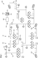
FIG. 1 shows a water supply network 100, which may be, for example, a municipal supply network for the supply of drinking or service water. The water supply network 100 comprises node components 105 and edge components 110, wherein an edge component 110 transports water between two node components 105.

Exemplary nodal components 105 include a tank 115, a water feeder 120, a water consumer 125, and a water distribution point 130. The water feeder 120, also referred to simply as feeder 120, typically includes a well, a source, or a delivery point other water network. A volume of water that flows from a feeder 120 into the water supply network 100 per time can usually not be influenced or only between predetermined limits. A water consumer 125 typically involves an end user, such as a private household, a commercial facility, or a public tapping point. How much water is withdrawn by the water consumer 125 from the water distribution network 100 can be at least approximately predicted, but an actual withdrawal can always deviate from a prognosis. A water distribution point 130 has n ports for edge components 110 and is also called an n-manifold or n-piece, where n is usually ≥ 2. For example, a T-shaped water distribution point 130 may also be called 3-manifold or 3-piece.

An edge component 110 may be controllable and in particular comprise a valve 135, a pump 140 or a turbine 145, or may not be controllable and may comprise approximately a pipeline 150. Among the controllable edge components 110, there are usually those which receive energy depending on their driving, in particular a pump 140, and those which absorb energy only during an adjustment, such as a valve 135, or are completely passive like the conduit 150. A pump 140 can only be switchable, so it can either be driven in a first operating configuration so that it operates and consumes energy, or it can not be driven in a second operating configuration so that it does not work and does not consume energy. It can also be a multi-stage or analog controllable in their performance pump 140 may be provided. In this case, the pump 140 may have more than two operating configurations. The performance of the pump can be done by controlling a particular electric drive or, for example, via the control of a coupling element such as a hydrodynamic torque converter. Infinitely controllable pumps 140 may also be provided by interval specifications for flow rate and Energy consumption in any number of different operating configurations are modeled and controlled.

A pump 140 may be powered by a utility 155, which typically includes a connection or transfer point of a utility grid. In some cases, the utility 155 may also include, for example, a local generator or other energy converter. A plurality of pumps 140 may be combined in a pumping station 160. In this case, the pumps 140 may be of a similar design, that is to say with the same pumping direction and pumping capacity, or different pumps 140 may be logically or physically enclosed. A turbine 145 operates substantially inversely with a pump 140, thus converting water flow into mechanical or electrical energy. Several turbines 145 may be combined in a turbine station 165, which may be formed analogous to a pumping station 160.

A controller 168 is provided to determine a control plan 170. The control device 168 preferably comprises a processing device, which may be designed in particular as a programmable microcomputer. The control plan 170 comprises a chronological sequence of activations of at least one controllable edge component 110 of the water supply network 100, in particular an edge component 110, which receives energy as a pump 140 depending on its activation. The control plan 170 is preferably a rough planning, ie does not lay down all aspects of Control of the water supply network in advance, but initially creates only a framework on the basis of which a control can be performed depending on current parameters of the water supply network 100, in particular on the basis of actual withdrawals, actual inflows and actual water levels in tanks 115th

The control plan 170 preferably relates to a predetermined planning horizon 175 that may be divided into individual time slices 180. The planning horizon 175 may be, for example one or more days, wherein a timeslice 180 may be, for example, one hour. The time slices 180 are preferably the same length and completely fill the planning horizon 175. The planning horizon 175 always extends into the future, so that with the advent of a time slice 180, a new time slice 180 can emerge in the farthest future within the planning horizon 175. The control plan 170 can only be determined for the newly added timeslice 180 or always for all time slices 180 of the planning horizon 175.
The water supply network 100 may be controlled based on a particular control plan 170. In one embodiment, one or more dedicated control devices are provided for this purpose, which may be arranged in particular in a decentralized manner, and to which preferably at least a part of the particular control plan is provided. In another embodiment, the controller 168 includes an interface 185 for connection to at least one of the controllable edge components 110 and is configured to provide a matching control signal to the edge component 110 via the interface 185.

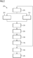
FIG. 2 FIG. 3 shows a flow chart of a method 200 for controlling a water supply network 100, such as that of FIG FIG. 1 , Individual steps of the method 200 may be performed in a sequence other than that indicated. In particular, the method 200 may be executed, in whole or in part, on the controller 168. For this purpose, the control device 168 may comprise a programmable microcomputer or microcontroller and the method 200 may be present at least partially in the form of a computer program product with program code means. The method 200 is tightly coupled to the controller 168 so that features or benefits may be transferred from the method 200 to the apparatus 168, or vice versa.

In a step 205, the planning horizon 175 and the time slices 180 are preferably determined. This provision may be repeated on subsequent runs of the method 200 or the previously determined result be adopted.

In a step 210, feed limits of the water feeders 120 are preferably determined. In particular, an upper and a lower limit can be determined, either for all water feeders 120 or for a group or a single water feed 120. In parallel, withdrawals by water consumers 125 are preferably determined or predicted. In particular, the prediction can be determined based on historical values or parameters such as an expected temperature or. The determinations of steps 210 and 215 are preferably performed for each of the time slices 180.

In a step 220, possible operating configurations can be determined. In this case, an operating configuration preferably comprises the configuration of an edge component 110 of the water supply network 100. The configuration may in particular comprise an activation state of a controllable edge component 110 and also an energy absorption of the edge component 110 or a flow through the edge component 110. The total of all possible operating configurations of all node components 110 may include Structure or architecture of the water supply network 100 logically reflect.

In step 225 energy costs may be determined. These may be dependent on a point in time, so that they can be determined individually for the time slices 180. Optionally, energy costs can also be determined by different providers, so that later a cheaper provider can be selected. The energy cost is relevant to the energy received by, for example, a pump 140 when it is energized to deliver water between node devices 105 of the water service network 100.

In a step 227, states of node components 105 per time slice may be determined. The node components 105 may in particular comprise a tank 105 and the state of the tank may relate to admissibility barriers at its filling or water level, z. B. maximum container volume or minimum level.

In a step 230, initial states of components of the water supply network 100 may be determined. As a result, an operating state of the water supply network 100 can be reflected. The initial states may include, for example, controls of components, positions of valves, or levels of tanks 115.

Steps 205-230 generally involve determining information necessary for the actual deployment of a control plan 170. In principle, the steps 205 to 230 can also be carried out in parallel or in any order.

Based on the collected information, in a step 235, the control plan 170 may be determined. The control plan 170 preferably includes all previously determined time slices 180. The specific determination of the control plan 170 is preferably carried out as an optimization within a search space which is predetermined by the restrictions described above. The optimization can be carried out in particular by means of a mixed-integer program, as will be explained in more detail below.

In a step 240, the particular control plan 170 may be provided, for example by being forwarded in parts or completely to a control device for controlling the water supply network 100. Alternatively, the control plan 170 may also be output to a person for control or reference, for example in numerical or graphical form.

In a step 245, the control plan 170, in particular in the context of a current time slice 180, can be performed by controlling the water supply network on the basis of the control plan 170. The control may be by means of the device 165 or other device. At the same time, a further rough planning can be carried out by repeating the method 200.

Hereinafter, an embodiment of the method 200 for controlling a water supply network will be detailed. In this case, a mathematical notation is used, which is particularly suitable for implementation by means of a mixed integer program, which, for example, with the aid of a commercial solver such. B. Scip, CPLEX or Gurobi can be solved in order to obtain optimized as a planning result values for the variables of the model. Mixed integer linear programs can be easily extended and adjusted, for example by additional constraints.

designations

For the definition of the mathematical model we introduce the following terms.

  Menge aller in die Knotenkomponente v eingehenden Kantenkomponenten e, d. h. bei positivem Fluss durch die Kantenkomponente e fließt das Wasser in die Knotenkomponente v hinein
$E_v^{-}$

  Menge aller aus der Knotenkomponente v ausgehenden Kantenkomponenten e, d. h. bei positivem Fluss durch die Kante e fließt das Wasser aus dem Knoten v heraus
E_v   Menge aller mit der Knotenkomponente v inzidenten Kantenkomponenten, d. h. $E_v=E_v^{+}\cup E_v^{-}$

C_e   Menge aller technischen Konfigurationen c, in denen die Kantenkomponente e betrieben werden kann. Eine Konfiguration legt dabei eine untere und eine obere Schranke für die zulässigen Flussraten fest (vgl. unten eingeführte Parameter ${\mathrm{\varphi }}_{e,c}^{\mathit{min}}$

und ${\mathrm{\varphi }}_{e,c}^{\mathit{max}})$

Quantities (identifier: Latin capital letters)
T = { t ₁ , t ₂ , ..., t _n } set of overlap-free and immediately adjacent time slices into which the planning horizon is divided; the indices correspond to the associated temporal sorting of these time slices, ie t ₁ denotes the first time slice, t _n the last one.
V Quantity of node components v in the water network (ie, the amount of all tanks, water feeders, water consumers, water distribution points, etc.)
E Amount of edge components e in the water network (ie amount of all pumps, valves, piping etc.)
$e_v^{+}$

The quantity of all edge components e coming into the node component v , ie, with positive flow through the edge component e , the water flows into the node component v
$e_v^{-}$

The set of all edge components e emanating from the node component v , ie, if there is a positive flow through the edge e , the water flows out of the node v
E _v set of all edge components incident to the node component v , ie $e_v=e_v^{+}\cup e_v^{-}$

C _e set of all technical configurations c in which the edge component e can be operated. A configuration defines a lower and an upper limit for the permissible flow rates (see parameters introduced below) ${\mathrm{\phi }}_{e.c}^{\mathit{min}}$

and ${\mathrm{\phi }}_{e.c}^{\mathit{Max}})$

  Zeitscheibe, die der Zeitscheibe t unmittelbar vorangeht $\left(t\in T\backslash \left\{t_1\right\}\right),$

d. h. ${\mathrm{\theta }}_{t_2}^{-1}=t_1$

${\sigma }_{v,t}^{\mathit{min}}$

  Minimal zulässiges gespeichertes Wasservolumen (gemessen z. B. in m³) in der Knotenkomponente v während der Zeitscheibe t und insbesondere auch zum Ende der Zeitscheibe t; für alle Knotenkomponenten, die keine Tanks sind, gilt stets ${\sigma }_{v,t}^{\mathit{min}}=0$

${\sigma }_{v,t}^{\mathit{max}}$

  Maximal zulässiges gespeichertes Wasservolumen (gemessen z. B. in m³) in der Knotenkomponente v während der Zeitscheibe t und insbesondere auch zum Ende der Zeitscheibe t; für alle Knotenkomponenten, die keine Tanks sind, gilt stets ${\sigma }_{v,t}^{\mathit{max}}=0$

${\sigma }_v^{\mathit{ini}}$

  Initial (d. h. zum Beginn des Planungshorizonts) gespeichertes Wasservolumen (gemessen z. B. in m³) in der Knotenkomponente v; für alle Knotenkomponenten, die keine Tanks sind, gilt stets ${\sigma }_v^{\mathit{ini}}=0$

${\mathrm{\rho }}_{v,t}^{\mathit{min}}$

  Minimale Wasser-Verbrauchsrate (gemessen z. B. in m³/s) für die Knotenkomponente ν während der Zeitscheibe t. Für Wasserverbraucher ist dieser Wert stets positiv, für Wassereinspeiser dagegen negativ. Bei negativen Werten dreht sich die Logik von "min" und "max" um. Für Tanks und Wasserverteilungspunkte gilt stets ${\mathrm{\rho }}_{v,t}^{\mathit{min}}=0$

${\mathrm{\rho }}_{v,t}^{\mathit{max}}$

  Maximale Wasser-Verbrauchsrate (gemessen z. B. in m³/s) für die Knotenkomponente v während der Zeitscheibe t (für Wasserverbraucher ist dieser Wert stets positiv, für Wassereinspeiser dagegen negativ. Bei negativen Werten dreht sich die Logik von "min" und "max" um. Für Tanks und Wasserverteilungspunkte gilt stets ${\mathrm{\rho }}_{v,t}^{\mathit{max}}=0$

${\mathrm{\kappa }}_e^{\mathit{ini}}$

  Initiale Betriebskonfiguration der Kantenkomponente e
${\mathrm{\varphi }}_{e,c}^{\mathit{min}}$

  Minimale Wasser-Flussrate (gemessen z. B. in m³/s) durch die Kantenkomponente e in der Betriebskonfiguration c (negative Werte kennzeichnen hier einen Wasserfluss entgegen der Orientierung der Kanten-Orientierung; will man dies vermeiden, so muss ${\mathrm{\varphi }}_{e,c}^{\mathit{min}}$

folglich nichtnegativ gewählt werden)
${\mathrm{\varphi }}_{e,c}^{\mathit{max}}$

  Maximale Wasser-Flussrate (gemessen z. B. in m³/s) durch die Kantenkomponente e in der Betriebskonfiguration c
${\mathrm{\omega }}_e^{\mathit{sw}}$

  Kostensatz pro Schaltung der Kantenkomponente e (≠ 0 nur für Pumpen)
${\mathrm{\omega }}_{e,t}^{\mathit{en}}$

  Kostensatz pro kWh Energie, die beim Betrieb der Kantenkomponente e während der Zeitscheibe t verbraucht wird
${\mathrm{\pi }}_{e,c}^{\mathit{min}}$

  Minimale elektrische Leistung (gemessen in kW) der Kantenkomponente e in der Betriebskonfiguration c, die zusammen mit der minimalen Flussrate ${\mathrm{\varphi }}_{e,c}^{\mathit{min}}$

anfällt; für Ventile und Rohre gilt stets ${\pi }_{e,c}^{\mathit{min}}=0$

${\mathrm{\pi }}_{e,c}^{\mathit{max}}$

  Maximale elektrische Leistung (gemessen in kW) der Kantenkomponente e in der Betriebskonfiguration c, die zusammen mit der maximalen Flussrate ${\mathrm{\varphi }}_{e,c}^{\mathit{max}}$

anfällt; für Ventile und Rohre gilt stets ${\mathrm{\pi }}_{e,c}^{\mathit{max}}=0$

Parameter (identifier: Greek lowercase and uppercase letters)
τ _t Duration of the time slice t (measured in s)
${\mathrm{\theta }}_t^{-1}$

Time slice immediately preceding the time slice t $\left(t\in T\backslash \left\{t_1\right\}\right).$

ie ${\mathrm{\theta }}_{t_2}^{-1}=t_1$

${\sigma }_{v.t}^{\mathit{min}}$

Minimum permissible stored water volume (measured, for example, in m ³ ) in the node component v during the time slice t and in particular also at the end of the time slice t ; for all node components that are not tanks, always applies ${\sigma }_{v.t}^{\mathit{min}}=0$

${\sigma }_{v.t}^{\mathit{Max}}$

Maximum permissible stored water volume (measured, for example, in m ³ ) in the node component v during the time slice t and in particular also at the end of the time slice t ; for all node components that are not tanks, always applies ${\sigma }_{v.t}^{\mathit{Max}}=0$

${\sigma }_v^{\mathit{ini}}$

Initial (ie at the beginning of the planning horizon) stored water volume (measured, for example, in m ³ ) in the node component v ; for all node components that are not tanks, always applies ${\sigma }_v^{\mathit{ini}}=0$

${\mathrm{\rho }}_{v.t}^{\mathit{min}}$

Minimum water consumption rate (measured eg in m ³ / s) for the node component ν during the time slice t . For water consumers, this value is always positive, but negative for water feeders. For negative values, the logic turns from "min" and "max". For tanks and water distribution points always applies ${\mathrm{\rho }}_{v.t}^{\mathit{min}}=0$

${\mathrm{\rho }}_{v.t}^{\mathit{Max}}$

Maximum water consumption rate (measured eg in m ³ / s) for the node component v during the time slice t (for water consumers this value is always positive, for water feeders it is negative.) For negative values the logic of "min" and "max." For tanks and water distribution points always applies ${\mathrm{\rho }}_{v.t}^{\mathit{Max}}=0$

${\mathrm{\kappa }}_e^{\mathit{ini}}$

Initial operating configuration of edge component e
${\mathrm{\phi }}_{e.c}^{\mathit{min}}$

Minimum water flow rate (measured, for example, in m ³ / s) by the edge component e in the operating configuration c (negative values indicate a flow of water contrary to the orientation of the edge orientation; ${\mathrm{\phi }}_{e.c}^{\mathit{min}}$

consequently not negatively selected)
${\mathrm{\phi }}_{e.c}^{\mathit{Max}}$

Maximum water flow rate (measured, for example, in m ³ / s) by the edge component e in the operating configuration c
${\mathrm{\omega }}_e^{\mathit{sw}}$

Cost rate per circuit of the edge component e (≠ 0 only for pumps)
${\mathrm{\omega }}_{e.t}^{\mathit{s}}$

Cost rate per kWh of energy consumed during operation of the edge component e during the time slice t
${\mathrm{\pi }}_{e.c}^{\mathit{min}}$

Minimum electrical power (measured in kW) of the edge component e in the operating configuration c , which together with the minimum flow rate ${\mathrm{\phi }}_{e.c}^{\mathit{min}}$

accrues; for valves and pipes always applies ${\pi }_{e.c}^{\mathit{min}}=0$

${\mathrm{\pi }}_{e.c}^{\mathit{Max}}$

Maximum electrical power (measured in kW) of the edge component e in the operating configuration c , which together with the maximum flow rate ${\mathrm{\phi }}_{e.c}^{\mathit{Max}}$

accrues; for valves and pipes always applies ${\mathrm{\pi }}_{e.c}^{\mathit{Max}}=0$

  Variable für die Dauer (gemessen in s), in der die Kantenkomponente e vor dem potentiellen Schaltvorgang der Komponente in Zeitscheibe t in der Zustands-Konfiguration c betrieben wird (e ∈ E, t ∈ T, c ∈ C_e )
$0\le d_{e,t,c}^2\le {\tau }_t$

  Variable für die Dauer (gemessen in s), in der die Kantenkomponente e nach dem potentiellen Schaltvorgang der Komponente in Zeitscheibe t in der Zustands-Konfiguration c betrieben wird (e ∈ E, t ∈ T, c ∈ C_e )
0 ≤ s_t ≤ τ_t   Variable für den potentiellen Schaltzeitpunkt (gemessen in s) der Kantenkomponenten während der Zeitscheibe t (t ∈ T). Da die Schaltungen für alle mit einer Knotenkomponente v inzidenten Kantenkomponenten zeitgleich erfolgen müssen und wir ohne Einschränkung der Allgemeinheit nur zusammenhängende Wassernetzwerke betrachten, ist der potentielle Schaltzeitpunkt für alle Kantenkomponenten stets derselbe. Die Variable ist daher nicht von e abhängig
$f_{e,t,c}^1$

  Variable für den Wasserfluss (gemessen z. B. in m³) durch die Kantenkomponente e vor dem potentiellen Schaltvorgang der Komponente in Zeitscheibe t in der Betriebszustands-Konfiguration c (e ∈ E, t ∈ T, c ∈ C_e )
$f_{e,t,c}^2$

  Variable für den Wasserfluss (gemessen z. B. in m³) durch die Kantenkomponente e nach einem möglichen Schaltvorgang der Komponente in Zeitscheibe t in der Betriebszustands-Konfiguration c (e ∈ E, t ∈ T, c ∈ C_e )
$g_{e,t,c}^1$

  Variable für den Energieverbrauch (gemessen in kWh) der Kantenkomponente e vor einem möglichen Schaltvorgang der Komponente in Zeitscheibe t in der Betriebszustands-Konfiguration c (e ∈ E, t ∈ T, c ∈ C_e ); der Energieverbrauch $g_{e,t,c}^1$

ist dabei mit dem zugehörigen Wasserfluss $f_{e,t,c}^1$

korreliert
$g_{e,t,c}^2$

  Variable für den Energieverbrauch (gemessen in kWh) der Kantenkomponente e nach dem potentiellen Schaltvorgang der Komponente in Zeitscheibe t in der Betriebszustands-Konfiguration c (e ∈ E, t ∈ T, c ∈ C_e ); der Energieverbrauch $g_{e,t,c}^2$

ist dabei mit dem zugehörigen Wasserfluss $f_{e,t,c}^2$

korreliert
$k_{e,t,c}^1\in \left\{0,1\right\}$

  Binär-Variable für die Entscheidung, in welcher Zustands-Konfiguration c die Kantenkomponente e vor dem potentiellen Schaltvorgang der Komponente in Zeitscheibe t betrieben wird (e ∈ E, t ∈ T, c ∈ C_e ); im Fall $k_{e,t,c}^1=1$

ist vor dem potentiellen Schaltvorgang die Konfiguration c aktiv, ansonsten eine andere Konfiguration c' ≠ c
$k_{e,t,c}^2\in \left\{0,1\right\}$

  Binär-Variable für die Entscheidung, in welcher Zustands-Konfiguration c die Kantenkomponente e nach dem potentiellen Schaltvorgang der Komponente in Zeitscheibe t betrieben wird (e ∈ E, t ∈ T, c ∈ C_e ); im Fall $k_{e,t,c}^2=1$

1 ist nach dem potentiellen Schaltvorgang die Konfiguration c aktiv, ansonsten eine andere Konfiguration c' ≠ c
0 ≤ m_e,t ≤ 1  Indikator-Variable, die anzeigt, ob es während der Zeitscheibe t bei der Kantenkomponente e zu einem Schaltvorgang kam oder nicht (e ∈ E, t ∈ T). Wenn ja, nimmt die Variable aufgrund der Nebenbedingungen automatisch den Wert 1 an, wenn nein den Wert 0. Man muss die Variable also nicht explizit als binär deklarieren
0 ≤ n_e,t ≤ 1  Indikator-Variable, die anzeigt, ob es beim Zeitscheibenübergang von der vorangegangenen Zeitscheibe ${\mathrm{\theta }}_t^{-1}$

zur Zeitscheibe t bei der Kantenkomponente e zu einem Schaltvorgang kam oder nicht (e ∈ E, t ∈ T\{t ₁}). Wenn ja, nimmt die Variable aufgrund der Nebenbedingungen automatisch den Wert 1 an, wenn nein den Wert 0. Man muss die Variable also nicht explizit als binär deklarieren
$u_{v,t}^1$

  Variable für den Wasserverbrauch (gemessen z. B. in m³) in der Knotenkomponente v vor dem potentiellen Schaltzeitpunkt während der Zeitscheibe t(v ∈ V, t ∈ T); ein negativer Wert für $u_{v,t}^1$

entspricht somit de facto einer Wassereinspeisung.
$u_{v,t}^2$

  Variable für den Wasserverbrauch (gemessen z. B. in m³) in der Knotenkomponente v nach dem potentiellen Schaltzeitpunkt während der Zeitscheibe t(v ∈ V, t ∈ T); ein negativer Wert für $u_{v,t}^2$

entspricht somit de facto einer Wassereinspeisung.
$w_{v,t}^{\mathit{end}}$

  Variable für das gespeicherte Wasservolumen (gemessen z. B. in m³) in der Knotenkomponente v zum Ende der Zeitscheibe t(v ∈ V, t ∈ T)
$w_{v,t}^s$

  Variable für das gespeicherte Wasservolumen (gemessen z. B. in m³) in der Knotenkomponente v zum Zeitpunkt des potentiellen Schaltzeitpunkts während der Zeitscheibe t(v ∈ V, t ∈ T) Variables (identifier: Latin lowercase letters)
$0\le d_{e.t.c}^1\le {\tau }_t$

Variable for the duration (measured in s), in which the edge component e is operated before the potential switching operation of the component in time slice t in the state configuration c ( e ∈ E, t ∈ T, c ∈ C _e )
$0\le d_{e.t.c}^2\le {\tau }_t$

Variable for the duration (measured in s), in which the edge component e is operated after the potential switching operation of the component in time slice t in the state configuration c ( e ∈ E, t ∈ T, c ∈ C _e )
0 ≤ s _t ≤ τ _t Variable for the potential switching time (measured in s) of the edge components during the time slice t ( t ∈ T ). Since the circuits for all incident with a node component v edge components must be done at the same time and we consider without restriction of generality only contiguous water networks, the potential switching time for all edge components is always the same. The variable is therefore not dependent on e
$f_{e.t.c}^1$

Variable for the water flow (measured, for example, in m ³ ) by the edge component e before the potential switching operation of the component in time slice t in the operating state configuration c ( e E, t E T, c E C _e )
$f_{e.t.c}^2$

Variable for the water flow (measured, for example, in m ³ ) by the edge component e after a possible switching operation of the component in time slice t in the operating state configuration c ( e E, t E T, c E C _e )
$G_{e.t.c}^1$

Variable for the energy consumption (measured in kWh) of the edge component e before a possible switching operation of the component in time slice t in the operating state configuration c ( e ∈ E, t ∈ T, c ∈ C _e ); the energy consumption $G_{e.t.c}^1$

is with the associated water flow $f_{e.t.c}^1$

correlated
$G_{e.t.c}^2$

Variable for the energy consumption (measured in kWh) of the edge component e after the potential switching operation of the component in time slice t in the operating state configuration c ( e ∈ E, t ∈ T, c ∈ C _e ); the energy consumption $G_{e.t.c}^2$

is with the associated water flow $f_{e.t.c}^2$

correlated
$k_{e.t.c}^1\in \left\{0,1\right\}$

Binary variable for the decision in which state configuration c the edge component e is operated before the potential switching operation of the component in time slice t ( e ∈ E, t ∈ T, c ∈ C _e ); in the case $k_{e.t.c}^1=1$

is the configuration c active before the potential switching operation, otherwise another configuration c ' ≠ c
$k_{e.t.c}^2\in \left\{0,1\right\}$

Binary variable for the decision in which state configuration c the edge component e is operated after the potential switching operation of the component in time slice t ( e ∈ E, t ∈ T, c ∈ C _e ); in the case $k_{e.t.c}^2=1$

1, the configuration c is active after the potential switching operation, otherwise a different configuration c ' ≠ c
0 ≤ m _{e, t} ≤ 1 Indicator variable indicating whether or not switching occurred during the time slice t for the edge component e ( e ∈ E, t ∈ T ) . If so, the variable automatically assumes the value 1 due to the constraints, if not the value 0. Therefore you do not need to explicitly declare the variable as binary
0 ≤ n _{e, t} ≤ 1 Indicator variable indicating whether it is at the time slicing transition from the previous time slice ${\mathrm{\theta }}_t^{-1}$

to the time slice t at the edge component e came to a switching process or not ( e ∈ E, t ∈ T \ { t ₁ }) . If so, the variable automatically assumes the value 1 due to the constraints, if not the value 0. Therefore you do not need to explicitly declare the variable as binary
$u_{v.t}^1$

Variable for water consumption (measured eg in m ³ ) in the node component v before the potential switching time during the time slice t ( v ∈ V, t ∈ T ); a negative value for $u_{v.t}^1$

thus corresponds de facto to a water feed.
$u_{v.t}^2$

Variable for the water consumption (measured eg in m ³ ) in the node component v after the potential switching time during the time slice t ( v ∈ V, t ∈ T ); a negative value for $u_{v.t}^2$

thus corresponds de facto to a water feed.
$w_{v.t}^{\mathit{end}}$

Variable for the stored volume of water (measured, for example, in m ³ ) in the node component v at the end of the time slice t ( v ∈ V , t ∈ T )
$w_{v.t}^s$

Variable for the stored water volume (measured eg in m ³ ) in the node component v at the time of the potential switching time point during the time slice t ( v ∈ V, t ∈ T )

Mathematical model in the form of a mixed-integer linear program

In the following, the constraints and the objective function of a mixed-integer linear program are gradually introduced. For this purpose, the required mathematical formulas are first defined in each case, an explanation of the associated logic for a better understanding is made in the connection.

unter den Nebenbedingungen (1), (2), ..., (24)With the formulas introduced, and taking into account value ranges of the variables, the following minimization problem arises: $$\mathrm{Minimize}\left(25\right)+\left(26\right)$$

under the constraints (1), (2), ..., (24)

Numerically referenced equations in this statement are described or derived in more detail below.

constraints

This section introduces the constraints of the mixed-integer program that define the allowed search space for the scheduling problem. Not all specified constraints must be met in all embodiments of the method and other or additional constraints may apply. $${\sigma }_{v.t}^{\mathit{min}}\le w_{v.t}^{\mathit{end}}\le {\sigma }_{v.t}^{\mathit{Max}}\left(v\in V.t\in T\right)$$

sorgt die Bedingung (1) dafür, dass nur in Tanks tatsächlich Wasser gespeichert werden kann. Für Tanks entspricht eine untere Schranke in der Regel einem Mindest- oder Sicherheitsfüllstand und eine obere Schranke einem physikalischen Fassungsvermögen. $${\sigma }_{v,t}^{\mathit{min}}\le w_{v,t}^s\le {\sigma }_{v,t}^{\mathit{max}}\left(v\in V,t\in T\right)$$

Secondary condition (1) defines for all end times of the time slices t a lower and an upper bound for the amount of water stored in the node component v . As applies to all node components except the tanks ${\mathrm{\sigma }}_{v.t}^{\mathit{min}}={\mathrm{\sigma }}_{v.t}^{\mathit{Max}}=0.$

Condition (1) ensures that only in tanks can water actually be stored. For tanks, a lower barrier usually corresponds to a minimum or safety level and an upper bound of physical capacity. $${\sigma }_{v.t}^{\mathit{min}}\le w_{v.t}^s\le {\sigma }_{v.t}^{\mathit{Max}}\left(v\in V.t\in T\right)$$

Secondary condition (2) analogously to (1) defines for all potential switching times of the edge components within all time slices t a lower and an upper limit for the amount of water stored in the node component v . These barriers correspond in our model without limitation of generality to those for the end times. $${\rho }_{v.t}^{\mathit{min}}\cdot s_t\le u_{v.t}^1\le {\rho }_{v.t}^{\mathit{Max}}\cdot s_t\left(v\in V.t\in T\right)$$

Secondary condition (3) defines for all time slices t and all node components v a lower and an upper bound for the water consumption averaged from the time step start to the potential switching time of the edge components in this node. The water consumption is measured on the basis of a product of rate and duration, for example in cubic meters. For tanks and N-pieces, the water consumption can be fixed to zero by the parameter specifications. For end users, the upper and lower bounds can be fixed to the respective predicted water consumption rates in the respective time step. Only with the feeders can thus result in real interval conditions that reflect the minimum and maximum water output of a water source. $${\rho }_{v.t}^{\mathit{min}}\cdot \left({\tau }_t-s_t\right)\le u_{v.t}^2\le {\rho }_{v.t}^{\mathit{Max}}\cdot \left({\tau }_t-s_t\right)\left(v\in V.t\in T\right)$$

Secondary condition (4) analogously to (3) defines for all time slices t and all node components v a lower and an upper bound for the water consumption averaged from the potential switching time of the edge components up to the time step end in this node. $${\phi }_{e.c}^{\mathit{min}}\cdot d_{e.t.c}^1\le f_{e.t.c}^1\le {\phi }_{e.c}^{\mathit{Max}}\cdot d_{e.t.c}^1\left(e\in e.t\in T.c\in C_e\right)$$

Secondary condition (5) defines for all time slices t , each edge component e and each associated operating configuration c a lower and upper bound for the respective water flow averaged by e from the time step beginning to the potential switching time of the edge components within the time step. The water flow is measured on the basis of a product of rate and duration, for example in cubic meters. Are pumps z. B. off (operating state "pump off"), the flow for this configuration using the barrier parameters is preferably fixed to zero. $${\phi }_{e.c}^{\mathit{min}}\cdot d_{e.t.c}^2\le f_{e.t.c}^2\le {\phi }_{e.c}^{\mathit{Max}}\cdot d_{e.t.c}^2\left(e\in e.t\in T.c\in C_e\right)$$

Secondary condition (6) analogously to (5) defines for all time slices t , each edge component e and each associated operating configuration c a lower and an upper bound for the respective water flow averaged by e from the potential switching time of the edge components up to the time step end. $$w_{v.t_1}^s={\sigma }_v^{\mathit{ini}}-u_{v.t_1}^1+\underset{e\in e_v^{+}}{\Sigma }\underset{e\in C_e}{\Sigma }{f}_{e.t_1.c}^1-\underset{e\in e_v^{-}}{\Sigma }\underset{e\in C_e}{\Sigma }{f}_{e.t_1.c}^1\left(v\in V\right)$$

das um die Durchflussmengen durch die in v eingehenden Kantenkomponenten bis zu diesem Zeitpunkt vergrößert und um den Wasserverbrauch des Knotens und die Durchflussmengen durch die aus v ausgehenden Kantenkomponenten bis zu diesem Zeitpunkt verringert wird. Zu beachten ist dabei, dass der Wasserverbrauch auch negativ sein kann, beispielsweise bei einem Einspeiser. Das Gleiche gilt unter Umständen auch für den Wasserfluss durch die Kantenkomponenten. Das jeweilige Vorzeichen sorgt dafür, dass die zugehörigen Wassermengen korrekt zur Wasser-Bilanz-Gleichung beitragen. Im Hinblick auf den Wasserfluss durch die Kantenkomponenten sei zusätzlich angemerkt, dass durch die Nebenbedingungen (10), (13) und (5) dafür gesorgt werden kann, dass es bei der Summierung über alle Betriebszustände jeweils nur höchstens einen Summanden ungleich null geben kann, da sich jede Kantenkomponente bis zum ersten Schaltzeitpunkt nur in einem einzigen Betriebszustand befinden kann. $$w_{v,t}^{\mathit{end}}=w_{v,t}^s-u_{v,t}^2+\sum _{e\in E_v^{+}}\sum _{e\in C_e}{f}_{e,t,c}^2-\sum _{e\in E_v^{-}}\sum _{e\in C_e}{f}_{e,t,c}^2\left(v\in V,t\in T\right)$$

Secondary condition (7) describes the water balance equation for all node components v from the start of the planning horizon (first time step) to the first potential switching time, which is usually within the first time slice. The volume of water stored in v at this first potential switching instant results from the initial volume ${\mathrm{\sigma }}_v^{\mathit{ini}}.$

up to this point in time, and by the water consumption of the node and the flow rates through the outgoing v out edge components until this time is reduced by the flow rates through the incoming edge components in v . It should be noted that the water consumption can also be negative, for example, in a feeder. The same may also apply to the flow of water through the edge components. The respective Sign ensures that the associated amounts of water contribute correctly to the water balance equation. With regard to the flow of water through the edge components, it should additionally be noted that the secondary conditions (10), (13) and (5) can ensure that, when summing over all operating states, there can only be at most one non-zero summand, since each edge component can only be in a single operating state by the first switching time. $$w_{v.t}^{\mathit{end}}=w_{v.t}^s-u_{v.t}^2+\underset{e\in e_v^{+}}{\Sigma }\underset{e\in C_e}{\Sigma }{f}_{e.t.c}^2-\underset{e\in e_v^{-}}{\Sigma }\underset{e\in C_e}{\Sigma }{f}_{e.t.c}^2\left(v\in V.t\in T\right)$$

Secondary condition (8) has the same balancing logic as constraint (7). However, it describes for all node components v and all time slices t the transition of the volume of water stored in v from the time of the potential switching time within the time slice to the end of the associated time slice. $$w_{v.t}^s=w_{v.{\theta }_t^{-1}}^{\mathit{end}}-u_{v.t}^1+\underset{e\in e_v^{+}}{\Sigma }\underset{e\in C_e}{\Sigma }{f}_{e.t.c}^1-\underset{e\in e_v^{-}}{\Sigma }\underset{e\in C_e}{\Sigma }{f}_{e.t.c}^1\left(v\in V.t\in T\backslash \left\{t_1\right\}\right)$$

bis zum potentiellen Schaltzeitpunkt der Nachfolger-Zeitscheibe t. $$k_{e,t,{\kappa }_e^{\mathit{ini}}}^1=1\left(e\in E\right)$$

Secondary condition (9) also has the same accounting logic as constraint (7). However, it describes for all node components v and all time slices t, with the exception of the first time slice, the transition of the water volume stored in v from the end time of the predecessor time slice ${\theta }_{\mathit{t}}^{-1}$

until the potential switching time of the successor time slice t . $$k_{e.t.{\kappa }_e^{\mathit{ini}}}^1=1\left(e\in e\right)$$

$$\sum _{c\in C_e}{k}_{e,t,c}^1=1\left(e\in E,t\in T\right)$$

Secondary condition (10) fixes the operating configuration for all edge components e at the beginning of the first time slice to the initial operating state ${\mathrm{\kappa }}_e^{\mathit{ini}}\mathrm{,}$

$$\underset{c\in C_e}{\Sigma }{k}_{e.t.c}^1=1\left(e\in e.t\in T\right)$$

um Binärvariablen handelt, die nur den Wert 0 oder 1 annehmen können, besagt Nebenbedingung (11), dass es stets genau eine eindeutig festgelegte Betriebs-Konfiguration c für jede Kantenkomponente e geben muss, die vom jeweiligen Beginn einer Zeitscheibe t bis zum zugehörigen potentiellen Schaltzeitpunkt innerhalb der Zeitscheibe aktiv ist. Alle anderen möglichen Betriebs-Konfigurationen der Kantenkomponente e bleiben somit in diesem Zeitraum inaktiv. $$\sum _{c\in C_e}{k}_{e,t,c}^2=1\left(e\in E,t\in T\right)$$

As it is the variables $k_{e.t.c}^1$

are binary variables that can only take the value 0 or 1, constraint (11) implies that there must always be exactly one clearly defined operating configuration c for each edge component e , from the respective beginning of a time slice t to the associated potential switching time within the time slice is active. All other possible operating configurations of the edge component e thus remain inactive during this period. $$\underset{c\in C_e}{\Sigma }{k}_{e.t.c}^2=1\left(e\in e.t\in T\right)$$

Secondary condition (12) is analogous to secondary condition (11), but deals with the time period from the potential switching time to the end of the respective time slice. Together with (11), (12) thus implies that in each time slice at most two operating configurations can be active, one each before and one after the potential switching time. If this is the same configuration, it can not effectively be switched and there is only one active configuration in that time slice. $$d_{e.t.c}^1\le {\tau }_t\cdot k_{e.t.c}^1\left(e\in e.t\in T.c\in C_e\right)$$

so ist diese Dauer automatisch auf 0 fixiert. Ist sie aktiv, so kann sie maximal die Länge der Zeitscheibe t betragen. Da aufgrund von (11) nur eine Konfiguration aktiv ist, kann somit auch höchstens einer Konfiguration eine positive Dauer zugeordnet werden. $$d_{e,t,c}^2\le {\tau }_t\cdot k_{e,t,c}^2\left(e\in E,t\in T,c\in C_e\right)$$

Secondary condition (13) represents for the first subsection of each time slice t , ie the time interval from the start to the potential switching time of the current time slice t , an upper limit for the duration over which the edge components e are located in the operating configuration c . If configuration c is not active in this period (ie $k_{e.t.c}^1=0).$

so this duration is automatically fixed to 0. If it is active, it can be at most the length of the time slice t . Since only one configuration is active due to (11), at most one configuration can therefore be assigned a positive duration. $$d_{e.t.c}^2\le {\tau }_t\cdot k_{e.t.c}^2\left(e\in e.t\in T.c\in C_e\right)$$

Secondary condition (14) is formulated analogously to secondary condition (13) and treats the respective second portion of each time slice t , that is to say from the potential switching time point to the end of the time slice. $$\underset{c\in C_e}{\Sigma }\left(d_{e.t.c}^1+d_{e.t.c}^2\right)={\tau }_t\left(e\in e.t\in T\right)$$

Secondary condition (15) ensures for all edge components e and all time slices t that the two durations of the active operating configurations of edge component e for the time periods before and after the potential switching time each add up to the total duration of the time slice, thus ensuring that exactly one operating configuration is active at any time in the planning horizon. $$s_t=\underset{c\in C_e}{\Sigma }{d}_{e.t.c}^1\left(t\in T\right)$$

$$m_{e,t}\ge k_{e,t,c}^2-k_{e,t,c}^1\left(e\in E,t\in T,c\in C_e\right)$$

Secondary condition (16) serves to determine the potential switching time for each time slice t . Because of (10) and (13), only a single one of the summands can be unequal to zero. The duration associated with this summation for the active time of the corresponding operating configuration corresponds to the switching time within the time slice, measured since the start of the time slice. $$m_{e.t}\ge k_{e.t.c}^1-k_{e.t.c}^2\left(e\in e.t\in T.c\in C_e\right)$$

$$m_{e.t}\ge k_{e.t.c}^2-k_{e.t.c}^1\left(e\in e.t\in T.c\in C_e\right)$$

und $k_{e,t,c}^2$

für alle Betriebs-Konfigurationen c denselben Wert und die untere Schranke besitzt den Wert 0. Fand hingegen eine Schaltung statt, so unterscheiden sich die Werte für die Variablen $k_{e,t,c}^1$

und $k_{e,t,c}^2$

genau für die beiden aktiven Betriebskonfigurationen. Die beiden Differenzen auf den rechten Seiten der Ungleichungen (17) und (18) betragen dann also 1 und -1, sodass sich insgesamt die untere Schranke 1 ergibt. Da in der Zielfunktion eine Schaltung mit Kosten belegt werden können, die dann zu minimieren sind, werden die Werte der Variablen m_e,t in der berechneten Lösung bevorzugt stets minimal gewählt, d. h. identisch mit der zugehörigen unteren Schranke. Somit ergibt sich aus der Optimierung, dass die Variablen m_e,t in der Optimallösung stets den Wert 0 oder den Wert 1 annehmen, ohne explizit als binär deklariert worden zu sein. $$n_{e,t}\ge k_{e,t,c}^1-k_{e,{\theta }_t^{-1},c}^2\left(e\in E,t\in T\backslash \left\{t_1\right\},c\in C_e\right)$$

$$n_{e,t}\ge k_{e,{\theta }_t^{-1},c}^2-k_{e,t,c}^1\left(e\in E,t\in T\backslash \left\{t_1\right\},c\in C_e\right)$$

The constraints (17) and (18) in combination represent a lower bound for the number of circuits within a time slice, ie, it is checked whether the edge component e at the potential switching time within the time slice t actually a circuit took place or not. If there was no circuit, then the variables have $k_{e.t.c}^1$

and $k_{e.t.c}^2$

For all operating configurations, c has the same value and the lower limit has the value 0. However, if a circuit was used, the values differ for the variables $k_{e.t.c}^1$

and $k_{e.t.c}^2$

exactly for the two active operating configurations. The two differences on the right-hand side of the inequalities (17) and (18) are then 1 and -1, so that the lower bound 1 results overall. Since in the objective function a circuit can be assigned costs which are then to be minimized, the values of the variables m _{e, t} in the calculated solution are preferably always chosen to be minimal, ie identical to the associated lower limit. Thus, it results from the optimization that the variables m _{e, t} in the optimal solution always assume the value 0 or the value 1, without being explicitly declared as binary. $$n_{e.t}\ge k_{e.t.c}^1-k_{e.{\theta }_t^{-1}.c}^2\left(e\in e.t\in T\backslash \left\{t_1\right\}.c\in C_e\right)$$

$$n_{e.t}\ge k_{e.{\theta }_t^{-1}.c}^2-k_{e.t.c}^1\left(e\in e.t\in T\backslash \left\{t_1\right\}.c\in C_e\right)$$

The constraint pair (19) and (20) have the same logic as the constraint pair (17) and (18). The difference lies in the fact that not the circuits within the time slices are checked, but the transition from the predecessor time slice to its successor time slice. Since an immediate switching of the initial operating configuration at time 0 is usually not provided (at most as a circuit "within" the time slice), the first time slice in the constraints (19) and (20) is respectively excluded. $$G_{e.t.c}^1={\pi }_{e.c}^{\mathit{min}}\cdot d_{e.t.c}^1\cdot \frac{1}{3600}\cdot \frac{H}{s}\left(e\in e.t\in T.c\in C_e:{\phi }_{e.c}^{\mathit{min}}={\phi }_{e.c}^{\mathit{Max}}\right)$$

Secondary condition (21) defines for each time slice t the energy consumption up to the potential switching time associated with the operation of the edge component e in the operating configuration c , if c prescribes a unique operating point, in particular with regard to a flow rate and thus also with respect to a performance. This is calculated from the product of the service belonging to c and the activity duration of this operating configuration. It should also be noted that the time unit must be converted from seconds to hours to indicate the energy in kWh. $$G_{e.t.c}^1=\left({\pi }_{e.c}^{\mathit{min}}\cdot d_{e.t.c}^1+\frac{{\pi }_{e.c}^{\mathit{Max}}-{\pi }_{e.c}^{\mathit{min}}}{{\phi }_{e.c}^{\mathit{Max}}-{\phi }_{e.c}^{\mathit{min}}}\cdot \left(f_{e.t.c}^1-{\phi }_{e.c}^{\min }\cdot d_{e.t.c}^1\right)\right)\cdot \cdot \frac{1}{3600}\cdot \frac{H}{s}\left(e\in e.t\in T.c\in C_e:{\mathrm{\phi }}_{e.c}^{\mathit{min}}\ne {\mathrm{\phi }}_{e.c}^{\mathit{Max}}\right)$$

Secondary condition (22) defines for each time slice t the energy consumption up to the potential switching time associated with the operation of the edge component e in the operating configuration c , if c instead of a unique operating point a true interval of possible operating points, in particular with respect to a flow rate and thus also with regard to a service.

passende Leistung angenommen wird, dass sie dieselbe relative Position innerhalb des Leistungsintervalls $\left[{\mathrm{\pi }}_{e,c}^{\mathit{min}},{\mathrm{\pi }}_{e,c}^{\mathit{max}}\right]$

einnimmt wie die zu $f_{e,t,c}^1$

gehörende Flussrate im Flussraten-Intervall $\left[{\mathrm{\varphi }}_{e,c}^{\mathit{min}},{\mathrm{\varphi }}_{e,c}^{\mathit{max}}\right]\mathrm{.}$

Liegt also die entsprechende Flussrate genau in der Mitte des zugehörigen Intervalls, dann liegt auch die Leistung in ihrem zugehörigen Intervall. Dieser Sachverhalt wird durch die in (22) enthaltene Geradengleichung umgesetzt. Aus der so ermittelten Leistung kann darüber hinaus durch Multiplikation mit der Dauer der zugehörige Energieverbrauch ermittelt werden. Dabei ist zu beachten, dass für $f_{e,t,c}^1$

diese Multiplikation bereits implizit in Nebenbedingung (5) erfolgt sein kann. Auch hier kann wobei analog zu (21) eine Umrechnung der Zeiteinheit von Sekunden in Stunden erforderlich sein, um die Leistung in kWh zu erhalten. $$g_{e,t,c}^2={\pi }_{e,c}^{\mathit{max}}\cdot d_{e,t,c}^2\cdot \frac{1}{3600}\cdot \frac{h}{s}\left(e\in E,t\in T,c\in C_e:{\mathrm{\varphi }}_{e,c}^{\mathit{min}}\ne {\mathrm{\varphi }}_{e,c}^{\mathit{max}}\right)$$

The idea behind the equation is that for the chosen flow rate $f_{e.t.c}^1$

matching power is assumed to have the same relative position within the power interval $\left[{\mathrm{\pi }}_{e.c}^{\mathit{min}},{\mathrm{\pi }}_{e.c}^{\mathit{Max}}\right]$

occupies like that $f_{e.t.c}^1$

associated flow rate in the flow rate interval $\left[{\mathrm{\phi }}_{e.c}^{\mathit{min}},{\mathrm{\phi }}_{e.c}^{\mathit{Max}}\right]\mathrm{,}$

So if the corresponding flow rate is exactly in the middle of the associated interval, then the power lies in their associated interval. This situation is implemented by the straight-line equation contained in (22). In addition, from the power determined in this way, the associated energy consumption can be determined by multiplying by the duration. It should be noted that for $f_{e.t.c}^1$

this multiplication already implicitly can be done in constraint (5). Again, analogous to (21), it may be necessary to convert the time unit from seconds to hours in order to obtain the power in kWh. $$G_{e.t.c}^2={\pi }_{e.c}^{\mathit{Max}}\cdot d_{e.t.c}^2\cdot \frac{1}{3600}\cdot \frac{H}{s}\left(e\in e.t\in T.c\in C_e:{\mathrm{\phi }}_{e.c}^{\mathit{min}}\ne {\mathrm{\phi }}_{e.c}^{\mathit{Max}}\right)$$

Secondary condition (23) is the analogue to secondary condition (21) for the period from the potential switching time to the end of the associated time slice t . $$G_{e.t.c}^2=\left({\pi }_{e.c}^{\mathit{min}}\cdot d_{e.t.c}^2+\frac{{\pi }_{e.c}^{\mathit{Max}}-{\pi }_{e.c}^{\mathit{min}}}{{\phi }_{e.c}^{\mathit{Max}}-{\phi }_{e.c}^{\mathit{min}}}\cdot \left(f_{e.t.c}^2-{\phi }_{e.c}^{\min }\cdot d_{e.t.c}^2\right)\right)\cdot \cdot \frac{1}{3600}\cdot \frac{H}{s}\left(e\in e.t\in T.c\in C_e:{\mathit{\phi }}_{e.c}^{\mathit{min}}\ne {\mathit{\phi }}_{e.c}^{\mathit{Max}}\right)$$

Secondary condition (24) is the analog of constraint (22) for the period from the potential switching time to the end of the associated time slice t .

objective function

This section defines the target function to be optimized. As already stated above, the objective function is based on a cost function that is to be minimized. $$\underset{e\in e}{\Sigma }{\omega }_e^{\mathit{sw}}\cdot \left(\underset{t\in T}{\Sigma }{m}_{e.t}+\underset{t\in T\backslash \left\{t_1\right\}}{\Sigma }{n}_{e.t}\right)$$

multipliziert und anschließend die Summe über alle Kantenkomponenten gebildet. De facto ist man jedoch nur an der Minimierung der Schaltungen von Pumpen interessiert und wählt daher bevorzugt ${\mathrm{\omega }}_e^{\mathit{sw}}=0$

für alle Kantenkomponenten, die keine Pumpen oder Turbinen sind. $$\sum _{c\in E}\sum _{t\in T}{\omega }_{e,t}^{\mathit{en}}\cdot \left(\sum _{c\in C_e}\left(g_{e,t,c}^1+g_{e,t,c}^2\right)\right)$$

Formula (25) describes the costs associated with the circuits of all edge components e . For this, for each edge component e, the number of all circuits determined with the variables m _{e, t} and n _{e, t} with the associated cost set ${\mathrm{\omega }}_e^{\mathit{sw}}$

multiplied and then formed the sum over all edge components. De facto, however, one is only interested in minimizing the circuits of pumps and therefore chooses preferred ${\mathrm{\omega }}_e^{\mathit{sw}}=0$

for all edge components that are not pumps or turbines. $$\underset{c\in e}{\Sigma }\underset{t\in T}{\Sigma }{\omega }_{e.t}^{\mathit{s}}\cdot \left(\underset{c\in C_e}{\Sigma }\left(G_{e.t.c}^1+G_{e.t.c}^2\right)\right)$$

und dann mit dem entsprechenden Energiekostensatz ${\mathrm{\omega }}_{e,t}^{\mathit{en}}$

multipliziert. Anschließend wird Summe über alle Einzelkosten in den jeweiligen Zeitschritten und für alle Kantenkomponenten gebildet, um die Gesamt-Energiekosten zu erhalten.Formula (26) describes the energy costs resulting from the operating strategy of the edge components. For this purpose, the energy consumption of each edge component e in each possible operating configuration c and in each time step t is calculated (this corresponds $G_{e.t.c}^1+G_{e.t.c}^2)$

and then with the corresponding one Energy cost rate ${\mathrm{\omega }}_{e.t}^{\mathit{s}}$

multiplied. Subsequently, the sum over all individual costs in the respective time steps and for all edge components is formed in order to obtain the total energy costs.

Expansion and customization options for new model variants

The approach of determining the operating strategy of a water supply network by means of a mixed-integer linear program offers the advantage of high flexibility, which is manifested in particular by a multiplicity of adaptation possibilities in the definition of secondary conditions and the design of a target function.

In the following, optional extensions of the procedure described above are briefly presented. The options are purely exemplary and represent a variety of possible variants and embodiments of the method. A detailed mathematical formulation is omitted in this section.

Synchronization of operating configurations of the edge components

Instead of optimizing the edge components individually as individual and independent components, it may be useful, for. B. Pumps in pumping stations for which also operating configurations can be defined. For example, for a pump station with three functionally identical pumps A, B and C, the configurations "all pumps off", "only pump A on", "pumps A and B on" and "all pumps on" can be defined. The introduction of such a pumping station can serve both to allow only technically meaningful state combinations of edge components, as well as help to save in the optimization of computer time, since z. B. equivalent state combinations of edge components (symmetries) can be avoided. The combinatorics of Under certain circumstances planning problems can be drastically reduced. A corresponding group formation is also conceivable for combinations of any other edge components.

Summary of several operating configurations in state classes

In addition to this idea of extension, a concrete operating configuration of the edge components can also be summarized in a condition class. For example, for a pumping station with three different pumps A, B and C, the condition class "exactly one pump is active" could be introduced, in which the three concrete operating configurations "only pump A is on", "only pump B is on" and " only pump C is to be summarized. This can also be very helpful in the definition of the technically meaningful combinations of operating configurations of the edge components for the reduction of the combinatorics.

Predefined active state classes

In some scheduling instances, it may be desirable not to give the optimizer full discretion over certain aspects of the solution. Instead, it may be desirable to predetermine some decisions already by a fixation or partial fixation. An example of this would be a maintenance of a pumping station, where all pumps must be switched off. In this case, the maintenance can be placed on one or more corresponding time slices and there operating configurations of all pumps can be predefined on "pump off". The same can be done for the condition classes described above. For example, it could simply be required for a pumping station that the status class "all pumps off" must be active in the time slices belonging to the maintenance. The associated state fixes or state fixes can then be given to the optimizer as additional constraints, so that these specifications must be taken into account in the optimization.

Differentiation of circuits

In the model introduced above, there is initially only a general type of circuit. In practice, it may be interesting that it is more important to avoid pump on / off circuits than to minimize circuitry between different operational operational configurations. This can also be integrated into the specified model by introducing different circuit variables, which are provided with correspondingly different cost rates in the target function.

water costs

Of course, the water consumption in the node components (in particular the feeders) can be evaluated by means of a cost function and integrated into the target function, so that the costs associated with the flow of water are also included in the optimization. This requires on the input side of data corresponding cost rates for water per volume at the different feeders. It also time series can be supported if the prices are not constant in time.

Turbines for energy production

In our model description, only three types of edge components have been introduced: pipes, valves and pumps. This approach can be easily extended by turbines. Turbines are interpreted as "inverse pumps" and thus allow the integration of an energy recovery option. The "energy consumption" associated with turbines is thus to be modeled negatively.

Total daily output of water sources

In addition to the water delivery rates dependent on the time slices, the total capacity for the water delivery of feeders, which is valid in the considered planning horizon, can also be modeled and included in the optimization, for B. by the specification of a maximum daily total delivery.

Restriction of energy availability

In the above model, the energy required to operate the pumps is assumed to be unlimited. Of course, upper limits for energy consumption can also be integrated into the model. For this purpose, for example, it would be possible to increase the allocation of the pumps to energy suppliers, which only guarantees a certain maximum delivery performance in the planning horizon.

Only tanks connected by pipes

Due to a lack of consideration of water pressures in the water supply network and the temporal aggregation, the presented model is a possibility for the rough planning of the water supply network or its control. Nevertheless, other physical conditions can be integrated into this model, the absence of which could otherwise lead to unrealistic planning results. An example of this are tanks that are connected to each other exclusively via pipes. In this case, additional conditions may be introduced to ensure that the level of these tanks must always be at the same level above sea level.

Analysis of inadmissible planning scenarios

The described mathematical model includes many upper and lower bounds that set the value ranges for the variables. It is therefore easy to create instances which do not have an acceptable solution because the chosen barriers do not match. In this case, so-called soft constraints can be made of the hard, ie unchangeable constraints by allowing a violation of the barriers, but this excess is charged at very high cost in the objective function. In this way it is possible, when planning a water supply network, a subnetwork or a component, to obtain a statement about which manipulated variables should be rotated in order, in the case of an inadmissible instance, to adapt to an operational system with as few adaptations as possible. To get architecture.

Although the invention has been further illustrated and described in detail by the preferred embodiment, the invention is not limited by the disclosed examples, and other variations can be derived therefrom by those skilled in the art without departing from the scope of the invention.

Claims (13)

A method (200) of controlling a water supply network (100) comprising node components (105) and edge components (110), wherein the edge components (110) transport water between the node components (105), wherein at least one of the edge components (110) has flow characteristics water controllable, and wherein the method (200) comprises the steps of: Determining (205) a planning horizon comprising a number of time slices; - determining (210) upper and lower limits for feeds of water into the water supply network (100) in the time slices; Determining (215) probable withdrawals of water from the water supply network (100) in the time slices; - determining (220) possible operational configurations of the at least one edge component (110); - determining (225) energy costs for driving the controllable edge components (110) in the time slices; - determining (227) allowable states of node components (105) of the water supply network (100); - determining (230) initial states of components (105, 110) of the water supply network (100); - determining (235) a control plan (170) for the at least one controllable edge component (110) based on the determined information such that a predetermined water balance of the water supply network (100) is maintained in each time slice (180) on average over time; - wherein the control plan (170) comprises a time sequence of activations of the at least one edge component (105); characterized in that - The control plan (170) a transition between different controls of the at least one edge component (110) allowed only once in each time slice and once at a transition from one time slice to the next. Method (200) according to claim 1, wherein the further transitions between different activations of several edge components (110) occur simultaneously. Method (200) according to claim 1 or 2, wherein the control plan (170) is created for a plurality of controllable edge components (110) and the time sequences of the activations of the edge components (110) are coordinated with one another. The method (200) of any of the preceding claims, wherein the control plan (170) is determined such that a quantity of water stored in a time slice (180) at a node component (105) in the node component (105) in a the preceding time slice (180) stored amount of water, plus an inflowing amount of water and less a draining amount of water. The method (200) of any one of the preceding claims, wherein an operating configuration comprises a permissible flow rate of water and allowable energy consumption of a controllable edge component (110). The method (200) of any of the preceding claims, wherein the node components (105) comprise a tank and a state of the tank relates to an interval of allowable levels. Method (200) according to one of the preceding claims, wherein the at least one edge component (110) comprises an active device (140) whose energy consumption depends on its activation and wherein the control plan (170) is determined such that the sum of the energy pickups of all edge components (110) over the entire planning horizon (175) is as small as possible. Method (200) according to one of the preceding claims, wherein the control plan (170) is determined in such a way that costs associated with the circuits of an edge component (110) are minimized as far as possible. Method (200) according to one of the preceding claims, wherein the at least one edge component (110) comprises at least one active device (140) and the time sequences of the activations of the edge components (110) are determined such that a total power of the active edge components (140 ) does not exceed a predetermined power. Method (200) according to one of the preceding claims, wherein one of the controllable edge components (110) comprises an active device (145) whose energy consumption can be negative. The method (200) of any of the preceding claims, wherein the control plan (170) is determined by a mixed-integer linear program. An apparatus (168) for controlling a water supply network (100) comprising node components (105) and edge components (110), wherein the edge components (110) transport water between the node components (105), wherein at least one of the edge components (110) has flow characteristics water controllable, and wherein the device (168) comprises processing means adapted to in a number of time slices (180) into which a planning horizon (175) is divided, - based on upper and lower limits for the supply of water to the water supply network (100) - and anticipated withdrawals of water from the water supply network (100) in the time slices; - possible operating configurations of the at least one edge component (110); - Energy costs for controlling the controllable edge components (110) in the time slices (180); permissible states of node components (105) of the water supply network (100); and Initial states of components (105, 110) of the water supply network (100) - Determine a control plan (170) for at least one of the controllable edge components (110) such that a predetermined water balance of the water supply network (100) is maintained in each time slice (180) in the time average; - wherein the control plan (170) allows a time sequence of transitions between different activations of the at least one controllable edge components (110) only once in each time slice (180) and once at a transition from one time slice (180) to the next. The apparatus (168) of claim 12, further comprising an interface (185) for connection to the at least one edge component (110), wherein the processing means (168) is adapted to drive the edge component (110) in response to the particular control plan (170) ,

Images