EP3086470A1 - Verfahren zum erstellen einer koppelmatrix zum abstimmen von filtern und vorrichtung zum abstimmen von filtern - Google Patents
Verfahren zum erstellen einer koppelmatrix zum abstimmen von filtern und vorrichtung zum abstimmen von filtern Download PDFInfo
- Publication number
- EP3086470A1 EP3086470A1 EP16162141.2A EP16162141A EP3086470A1 EP 3086470 A1 EP3086470 A1 EP 3086470A1 EP 16162141 A EP16162141 A EP 16162141A EP 3086470 A1 EP3086470 A1 EP 3086470A1
- Authority
- EP
- European Patent Office
- Prior art keywords
- matrix
- coupling matrix
- filter
- current
- similarity transformation
- Prior art date
- Legal status (The legal status is an assumption and is not a legal conclusion. Google has not performed a legal analysis and makes no representation as to the accuracy of the status listed.)
- Granted
Links
Images


Classifications
-
- H—ELECTRICITY
- H03—ELECTRONIC CIRCUITRY
- H03H—IMPEDANCE NETWORKS, e.g. RESONANT CIRCUITS; RESONATORS
- H03H7/00—Multiple-port networks comprising only passive electrical elements as network components
- H03H7/01—Frequency selective two-port networks
- H03H7/0153—Electrical filters; Controlling thereof
-
- H—ELECTRICITY
- H03—ELECTRONIC CIRCUITRY
- H03H—IMPEDANCE NETWORKS, e.g. RESONANT CIRCUITS; RESONATORS
- H03H7/00—Multiple-port networks comprising only passive electrical elements as network components
- H03H7/01—Frequency selective two-port networks
- H03H7/0123—Frequency selective two-port networks comprising distributed impedance elements together with lumped impedance elements
-
- H—ELECTRICITY
- H03—ELECTRONIC CIRCUITRY
- H03J—TUNING RESONANT CIRCUITS; SELECTING RESONANT CIRCUITS
- H03J1/00—Details of adjusting, driving, indicating, or mechanical control arrangements for resonant circuits in general
- H03J1/0008—Details of adjusting, driving, indicating, or mechanical control arrangements for resonant circuits in general using a central processing unit, e.g. a microprocessor
-
- H—ELECTRICITY
- H03—ELECTRONIC CIRCUITRY
- H03J—TUNING RESONANT CIRCUITS; SELECTING RESONANT CIRCUITS
- H03J3/00—Continuous tuning
-
- H—ELECTRICITY
- H04—ELECTRIC COMMUNICATION TECHNIQUE
- H04B—TRANSMISSION
- H04B3/00—Line transmission systems
- H04B3/02—Details
- H04B3/04—Control of transmission; Equalising
-
- H—ELECTRICITY
- H01—ELECTRIC ELEMENTS
- H01P—WAVEGUIDES; RESONATORS, LINES, OR OTHER DEVICES OF THE WAVEGUIDE TYPE
- H01P1/00—Auxiliary devices
- H01P1/20—Frequency-selective devices, e.g. filters
- H01P1/207—Hollow waveguide filters
- H01P1/208—Cascaded cavities; Cascaded resonators inside a hollow waveguide structure
Definitions
- the present application relates to a device for tuning tuners of filters and corresponding methods.
- the present application describes a method with which a coupling matrix can be created with less time and computation effort.
- the coupling matrix created in this way can reproduce the physical structure of a filter to be matched very precisely.
- resonator filters i.a. Waveguide filters must, after manufacture or during operation, e.g. Adaptive filters for cognitive radio applications, are tuned to meet the specified specifications.
- the task of tuning is to adjust the couplings and resonance frequencies of the resonators. Due to the complexity of the interaction of these parameters, the coordination is difficult and so far associated with high time / computational effort.
- Known approaches for tuning filters have, in particular, disadvantages with regard to the effort required for the tuning or the preparation of the voting devices, the convergence and / or the mapping of the physical structure of the filter by means of coupling matrices.
- the method should have good convergence properties, require less computation and time and create a coupling matrix that maps the physical structure of the filter as accurately as possible. In terms of computation and time, it would be particularly advantageous if the method requires no training for predetermined filter, since then there is also a better flexibility in terms of tuning different filters.
- a method for creating a matched coupling matrix of a filter or for mapping a physical structure of a filter may include the steps of measuring scattered parameter data of the filter, approximating the measured scattering parameter data using rational functions, constructing an original coupling matrix based on the rational functions, and constructing a matched coupling matrix that maps the physical structure of the filter based on the original coupling matrix.
- the last step may also be referred to as adapting / reconfiguring the coupling matrix to be matched to the physical structure of the filter (the coupling matrix to be adapted can be iteratively adapted or created starting from the original coupling matrix).
- the measurement of the scattering parameter data may include measuring a filter to be tuned by means of a network analyzer.
- the scattering parameter data can be measured particularly preferably as a function of the frequency.
- the scattering parameter data may include, for example, the measured values of a two-port; but also play more complex circuits.
- An example of the step of approximation may include that the scattering parameters are transformed into Y-parameters, for example, and then further processed, for example, by means of the method "vector fitting” (the “vector fitting” is described by, for example) Gustavsen and A. Semlyen, “Rational approximation of frequency domain responses by vector fitting", IEEE Trans. Power Del., Vol. 14, no. 3, 1999 ). Other algorithms or methods can also be used.
- the approximation can be preceded by an optional step "deembedding the measured data" to further increase the reliability and accuracy of the method. Deembeding is especially preferred when the approximation is performed on a model of rational functions of low order (eg, smaller N), since these models do not time delays at the filter gates (not exactly enough) can map; It should be noted that the order of the rational model should be equal to the order of the real filter in order to obtain a physically meaningful model. In a model with low-order rational functions, it is possible to improve the accuracy of the mapping by "de-embedding" possible time delays. Preferably, the "deembedding" is carried out by known methods.
- the creation of the (original) coupling matrix (which generally does not yet represent the physical structure of the measured filter) from the rational functions can be done in different ways.
- a preferred example for the creation of the coupling matrix is, for example, of V. Miraftab and M. Yu "Advanced Coupling Matrix and Admittance Function Synthesis Techniques for Dissipative Microwave Filters” in IEEE TRANSACTIONS ON MICROWAVE THEORY AND TECHNIQUES, VOL. 57, NO. 10, pp. 2429-2438 (October 2009 ).
- the result is a fully populated coupling matrix with complex values.
- the real parts of the values describe capacitive and inductive couplings of the resonators of the filter, as well as self-coupling effects.
- the coupling matrix generated to date does not yet reflect the real topology of the filter and is therefore still being adapted or reconfigured in this respect according to the method described here.
- the first step is the creation of an original coupling matrix, followed by the step of adapting to the topology of the measured filter.
- the coupling matrix values of the original coupling matrix are correlated with the measured values.
- step of creating a coupling matrix from the rational functions first provides an original coupling matrix, hereinafter denoted by "L”.
- step of creation or reconfiguration or adaptation then provides a customized coupling matrix, marked with "M”, which reflects the physical structure of the filter.
- the adjusted coupling matrix is changed during the adaptation / reconfiguration, but the originally created coupling matrix is not.
- the result of the method described here is the adapted coupling matrix ("M") whose (initial) structural deviation from a given structure can be minimized iteratively.
- the procedural reconfiguration or adaptation of the original coupling matrix makes it possible that the physical structure of the filter can be replicated very accurately and with less time and computational effort. Good convergence is achieved.
- the method described here has the advantages that the topology of the filter can be mapped very accurately and high convergence is achieved.
- the time and computation effort for the adaptation of the coupling matrix is also reduced by not generating a training overhead or the like, e.g. in approaches with neural networks is required.
- the step of creating the adapted coupling matrix may comprise iteratively a structure deviation indicating a deviation between the adapted coupling matrix (hereinafter also referred to as "coupling matrix" as distinguished from “original coupling matrix”) and a physical structure of the filter to be mapped is minimized.
- a structure matrix can be given which can reproduce the physical structure of the filter to be imaged.
- the structure deviation can be determined on the basis of the (adapted) coupling matrix and the structure matrix.
- the structural deviation can be determined from a difference between (adapted) coupling matrix and structure matrix.
- the structural deviation may preferably be a scalar that indicates a difference between the coupling matrix and a structure matrix or a coupling matrix that was calculated with the structure matrix.
- “Iterative minimization” should particularly preferably include that the structural deviation or its value is minimized in recurrent loop passes of sub-steps of the reconfiguration-preferably as far as possible until a global or at least local minimum could be found.
- the structure matrix may be a binary matrix, that is, constructed to contain only "0" and "1" as element values.
- the structure matrix may preferably have the preferred and predetermined matrix structure of the coupling matrix.
- the structure matrix preferably has elements with value "0” placed in such a way that at this point the elements of the coupling matrix disappear during the reconfiguration.
- a "1" can be provided at these locations of the structure matrix, where couplings and the like of the coupling matrix should be preserved.
- the deviation between the desired physical structure of the filter and the coupling matrix is represented by the structure deviation value. This value thus indicates how well the current (during the iteration) coupling matrix already corresponds to the desired, final adapted coupling matrix (as the desired product of the iteration / reconfiguration).
- the operator " ⁇ ” denotes an elemental product (Frobenius product).
- an index can be used to distinguish current values from current matrices and values / matrices that are / were current in an iteration run before or after.
- the equation given above (as well as the other equations used here) can be provided with indices accordingly.
- the present method thus makes it possible to calculate a quality parameter that can be evaluated with little effort, the structural deviation, which indicates the quality of the coupling matrix with regard to the topology of the filter to be mapped and which can be minimized iteratively.
- the step of creating the adapted coupling matrix may comprise the substeps of: determining a current iteration solution (or modification) of the adapted coupling matrix M based on an actual (modification of) the similarity transformation matrix Q and the original coupling matrix, and / or determining a current one Iteration solution of the structural deviation ⁇ .
- the values M i , Q i and ⁇ i should be used or calculated here.
- the coupling matrix M i is modified further during the iterations to finally achieve the desired minimization of the structural deviation.
- the original coupling matrix (or a matrix-decomposed sub-matrix of this), which was obtained from the rational functions and does not yet reproduce the topology of the filter, becomes constant and unchanged.
- test steps may be provided which check the achievement / fulfillment of predetermined termination conditions and, if necessary, determine the termination or the end of the minimization.
- a step for increasing i by the value "1" can be provided after each loop pass. Particularly preferably, this step of increasing i take place after the test procedure. Additional steps to increase i may optionally be provided.
- an advantage of the aspect of the method described herein is that the original coupling matrix is decomposed so that the similarity transformation matrix can be obtained, which can then be varied / modified.
- the similarity transformation matrix may be a rotation matrix.
- Previously known methods vary the originally created coupling matrix itself, which leads to undesirable effects with regard to the scattering parameters, since these are changed when the coupling matrix changes itself, so that the computation and time expenditure increases and the convergence becomes worse.
- a variety of boundary conditions must be adhered to during the optimization of the scattering parameters. This is advantageously not necessary in the method described here, which envisages the optimization of the similarity transformation matrix, since the scattering parameters remain unchanged.
- the similarity transformation matrix may be constructed to have the property not to alter the measured scattering parameters during the iteration / reconfiguration.
- the arrangement of the filter poles and zeroes may be invariant with respect to the modification of the similarity transformation matrix during the minimization of the pattern deviation.
- determining a current (modification of) the similarity transformation matrix based on a gradient g of the previously current similarity transformation matrix and a predetermined one Step size ⁇ are performed.
- the minimization of the structural deviation can be performed with relatively little computational effort by means of a gradient method.
- the use of a gradient method to minimize structural deviation is a particularly preferred option of the method described herein.
- alternative methods for minimizing the structural deviation can also be used, for example, a genetic algorithm for minimizing the structural deviation can also be used.
- the above modification of the similarity transformation matrix may be based on a gradient of the formerly current similarity transformation matrix from a second iteration / run, i. for example, be carried out from an iteration with i ⁇ 2.
- the second and subsequent (modification (s) of the) similarity transformation matrices can be calculated in this way.
- i 1, i. for a first similarity transformation matrix, a starting value may preferably be given, i. the first similarity transformation matrix may be obtained other than the equation below, e.g. through a matrix decomposition of L.
- the new current or further modification of the similarity transformation matrix can be calculated such that the previously valid similarity transformation matrix and the gradient of this previously valid similarity transformation matrix are used for the calculation.
- the parameter ⁇ can be freely selectable and specify a step size which determines how far during an iteration run in the direction of the gradient should be gone.
- a starting value for ⁇ is already predetermined or input at the start of the adaptation of the coupling matrix.
- the gradient is preferably recalculated for each pass, ie one step at a time can be provided for the calculation of g during an iteration run, which can be particularly preferably arranged before the calculation of the next modification of the similarity transformation matrix.
- the gradient g can optionally and alternatively also be kept as a constant over the iterations, if it had been determined once after the first pass. In this case, the equations concerned must be adjusted so that a constant is used for the gradient.
- the constant gradient g according to the above-mentioned optional alternative can be used with particular preference during optimization as long as steps in the direction of the gradient still lead to a smaller structural deviation. If this condition is no longer met, the gradient should be adjusted or redefined.
- f m, n denote the individual elements of the matrix f.
- the sub-step for calculating f m, n must be performed frequently according to the number of elements of f. For example, for an N * N matrix, N 2 times.
- the matrix V is an auxiliary quantity.
- L is the original coupling matrix.
- S is the matrix of the physical filter structure to be achieved.
- the matrix J m, n is constructed such that all but the m, n element which is "1", all other elements are "0".
- the method may further comprise: comparing the current iteration solution of the structural deviation ⁇ with a predetermined limit ⁇ limit , and / or comparing the (current) step size ⁇ with a predetermined limit value ⁇ limit .
- a predetermined limit value can be specified as desired. Preferably, however, very small values are set in order to ensure the highest possible accuracy. Values of ⁇ limit ⁇ 10 -5 are preferred, more preferably ⁇ limit ⁇ 10 -10 , and most preferably ⁇ limit ⁇ 10 -12 is set.
- the comparison of the step size for the current iteration run with a predetermined limit ⁇ limit can preferably be made after each adaptation of the similarity transformation matrix or each calculation of the coupling matrix M.
- the threshold for the step size is preferably ⁇ limit ⁇ 10 -1 , more preferably ⁇ limit is set to ⁇ 10 -4 . Most preferably, ⁇ limit ⁇ 10 -5 is set.
- the advantage of checking the step size is that local minima can be identified.
- the minimization of the structural deviation can be terminated in at least two different conditions.
- the minimization can be ended if the current value for ⁇ falls below the limit ⁇ limit .
- the minimization may be terminated if the current step size is less than ⁇ limit . In the latter case, it is reliably and reliably determined that a local minimum was found.
- the method may comprise querying whether the current structural deviation is greater than that of the preceding iteration step, particularly preferably if the structural deviation is greater than the predetermined limit value and / or the increment ⁇ is greater than the predetermined limit value. Most preferably, the two structural deviations of the current and previous run are compared with each other when both the structural deviation is greater than the predetermined threshold and the step size ⁇ is greater than the predetermined threshold. This further check request can ensure that actually a minimization takes place.
- a further sub-step may be provided.
- This may include "undoing the last step," which may specifically include undoing the (last, previous) adaptation / modification of the similarity transformation matrix.
- this may mean that the similarity transformation matrix is reset to its previous state or that the current modification of the similarity transformation matrix is recalculated with a new increment.
- the step size ⁇ can also be adapted and, with particular preference, reduced in size.
- the step size ⁇ can be reduced in size automatically. It can be provided, for example, that the increment ⁇ is automatically halved, reduced by one power of ten or changed in another way. However, a manual adjustment can also be provided.
- the method may include resetting the similarity transformation matrix to the previous iteration step and decreasing the step size ⁇ if the current / last pattern deviation is greater than that of the previous iteration step. This allows to ensure that the minimization is not in the "wrong Direction, and in fact minimizing the structural deviation, thus further increasing the safety of the method in terms of the reliability of the results and the convergence.
- indices for distinguishing the iterations
- the iteration may be terminated when a (current) structural deviation is less than the predetermined threshold and / or (most preferred is the "or" option), the (current) increment ⁇ is less than the predetermined threshold.
- the end of the minimization is determined securely detectable.
- the start of the iteration can be based thereon or the first iteration solution of the coupling matrix M 1 can be determined by means of a first similarity transformation matrix, which can result from a matrix decomposition of the original coupling matrix L.
- the first similarity transformation matrix may be the shape 1 0 ... 0 0 0 ⁇ Q innnen T ⁇ 0 0 0 0 ... 0 1 exhibit.
- the inner matrix (submatrix) Q INNEN may be a similarity transformation matrix.
- the above-mentioned form of the similarity transformation matrix may indicate the most general form with which the method presented here so it is feasible that the scatter parameter values are not changed during minimization.
- the good convergence can advantageously be achieved here and at the same time it can be prevented that the method for adapting the coupling matrix leads to complex arithmetic operations and, if necessary, the result could not be accurate enough.
- the above-mentioned form of the similarity transformation matrix has two preferred properties: The generalized eigenvalues of the matrix pencil (L, I) remain unchanged during the transformation or matrix decomposition. The eigenvalues are equal to the transmission poles of the filter. This property is achieved by the similarity transformation matrix describing a similarity transformation. Furthermore, the transmission and reflection "zeros" remain unchanged during the transformation. The position of these zeros is affected by the eigenvalues of corresponding minor. This property is achieved by transforming the minor similarity transformations as well.
- the determination of the first iteration solution of the coupling matrix M 1 can be carried out by means of the unit matrix I as the first (start) similarity transformation matrix Q 1 .
- the first iteration solution of the coupling matrix M 1 can be determined such that the original Coupling matrix is decomposed by means of a generalized eigenvalue decomposition with the matrix tuft (L, I), so that the resulting transformation matrix has the form given above 1 0 ... 0 0 0 0 ⁇ Q innnen T ⁇ 0 0 0 0 ... 0 1 receives.
- the decomposition and subsequent change of the similarity transformation matrix during the minimization of the structural deviation has the advantage that the scattering parameter values are not changed during the minimization.
- orthonormalization of the modified similarity transformation matrix may be performed after the modification of the similarity transformation matrix.
- This preferred further step can prevent that small deviations of the similarity transformation matrix after its adaptation along the gradient in the step before, can be compensated.
- the Gram-Schmidt method for the orthonormalization of the adapted similarity transformation matrix is particularly preferably carried out here. The accuracy of the method can thus be further increased.
- the step S5 indicated in the figures may comprise the substeps (wherein the equations given above with corresponding indices "i" can be used for the corresponding steps): determining a first coupling matrix M 1 based on a predetermined first similarity transformation matrix Q. 1 , which is the identity matrix, and the original coupling matrix from step S4. Calculating the first structure deviation based on the first coupling matrix M 1 . Check (optional) if the first structure deviation is smaller than a specified limit value. If not, a first gradient g 1 is calculated and i is increased to the value "2".
- the Modification of the similarity transformation matrix Q 2 orthonormalized.
- the further modified coupling matrix M i (using Q i and the original coupling matrix) and the further modified structure deviation ⁇ i is calculated and checked as to whether the further modified structure deviation ⁇ i is smaller than the predetermined limit value. If this is not the case, it is checked whether the increment used for the calculation of the modification of the similarity transformation matrix was small enough. If this is not the case, it is checked whether the current value of the structure deviation is greater than the previously valid value.
- the checking steps may also be deviating, e.g. in a different order.
- the step size can first be checked before the structural deviation is compared with a limit value.
- the further modified coupling matrix M i + 1 (by Q i + 1 and the original coupling matrix) and the further modified structure deviation ⁇ i + 1 is calculated and checked whether the further modified structure deviation ⁇ i + 1 is smaller than the predetermined limit value. If this is not the case, it is checked whether the increment used for the calculation of the modification of the similarity transformation matrix was small enough. If this is not the case, it is checked whether the current value of the structure deviation is greater than the previously valid value. If so, the similarity transformation matrix is reset and recalculated at a reduced increment. If not, i is increased by the value "1" and a further modified value of the gradient g i is determined.
- a method may also be provided for tuning a filter which may use the matched coupling matrix to tune the filter made by a method according to at least one of the preceding aspects. More preferably, the above-discussed method aspects for tuning a filter may thus be incorporated into a method that uses the coupling matrix after tuning to set / tune a filter.
- a device for creating a matched coupling matrix of a filter and / or for tuning a filter by means of a matched coupling matrix may be provided here.
- the means for establishing the matched coupling matrix may include: one or more means for measuring scattering parameter data of the filter, one or more means for approximating the measured scattering parameter data by means of rational functions, one or more means for constructing the original coupling matrix based on the rational functions, and / or to create the adapted coupling matrix (which is adapted to the physical structure of the filter).
- the device for tuning the filter may include the means for establishing the matched coupling matrix and one or more means for tuning the filter based on the matched coupling matrix.
- the means for tuning the filter may be, for example, a tuning screw or the like. Tuning can be automated or manual.
- the means for measuring scatter parameter data may be a network analyzer.
- the means for approximating, creating the coupling matrices may be one or more computers / computers.
- a computer program product may be provided with computer program means that may be stored on a computer readable medium and executable by a computer, wherein the computer program means may include executable instructions that may cause the computer to perform the steps of at least one of to carry out the aforementioned method aspects.
- a method is presented here which has good convergence, generates less computational effort and can reproduce very accurately the physical structure of the filter to be matched by means of a matched coupling matrix. Furthermore, a corresponding device for carrying out the method for tuning the filter and / or for adapting the coupling matrix and a corresponding computer program product are described.
- a higher reliability and speed of the method can thus be achieved by means of the method (s) described here, the device (s) and the corresponding computer program products.
- This allows the use of appropriate adaptive filters in multifunctional and / or cognitive radio systems in which built-in electrical or mechanical tuning elements are automatically adjusted in quasi-real-time to the requirements of the application.
- higher productivity can be achieved after production due to reduced time requirements.
- the general applicability of the method eliminates the expense of prior training of a specialized algorithm (such as neural networks).
- the method can also be used for lossy filters.
- Fig. 1a shows first generally the structure of a filter F, for example with three resonators (nodes 1, 2 and 3). These resonators are coupled with each other with the coupling strength c xy (drawn edges).
- the structure graph can be represented equivalently as a parameter set in the form of a matrix, the so-called coupling matrix L.
- FIG. 1b shows a coupling matrix L which is the structure graph of FIG. 1a corresponding maps.
- the diagonal entries f1 to f3 here describe a possible deviation of the resonant frequency of the resonator from the center frequency.
- the entries can also be equal to "0".
- the corresponding couplings or coupling strengths c xy the FIG. 1a are entered element by element in the matrix.
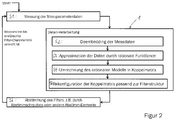
- FIG. 2 shows an example of a sequence of steps or a process for tuning a filter F.
- This method also includes a method for creating a coupling matrix M, which reflects the topology of the filter F.
- the scatter parameter data are measured here (step S1).
- a network analyzer A see FIG. FIG. 5 ) are used, with which the tuned filter F is measured.
- the measured scattering parameter data in a device for data processing, for example.
- a computer 1 (s. FIG. 5 ). This can be done via a data line or wireless connection or manually, for example by means of transport and dubbing on / from a storage means.
- the data processing then includes, as exemplified in FIG. 2 is shown, first a step S2, which is referred to as "deembedding" of the measurement data.
- the measured scatter parameter data may include time delays that are different from a Time delays may originate at the gates of the filter. By means of “deembedding" these time delays can be removed.
- the "deembedding" can be carried out by means of known methods and is preferably carried out in the cases in which models of rational functions with low order are used in step S3, since these models can not reliably map time delays.
- step S3 the already mentioned mapping or approximation of the scatter parameter data takes place by means of rational functions.
- first of all Y-parameters can be obtained from the scattering parameter data, from which the rational functions can then be determined by means of rational approximation.
- a previously known algorithm for the rational approximation used in step S3 is the "vector fitting algorithm” (eg. Gustavsen and A. Semlyen, "Rational approximation of frequency domain responses by vector fitting", IEEE Trans. Power Del., Vol. 14, no. 3, 1999 ).
- vector fitting algorithm eg. Gustavsen and A. Semlyen, “Rational approximation of frequency domain responses by vector fitting", IEEE Trans. Power Del., Vol. 14, no. 3, 1999.
- Other algorithms or methods can also be used.
- step S4 is carried out, which provides for a conversion of the rational model / functions into an original coupling matrix L.
- This conversion or the extraction of the original coupling matrix L can preferably by means of the V. Miraftab et. al. in "Generalized lossy microwave filter coupling matrix synthesis and design using mixed technologies" in IEEE Transactions on Microwave Theory and Techniques, vol. 56, no. 12, December 2008 described method. Other algorithms or methods can also be used.
- step S4 is therefore the original coupling matrix L, which, however, does not yet reflect the physical structure of the filter to be tuned and is therefore not yet suitable for the highly accurate tuning / tuning of a filter. Therefore, according to the method, a further step S5 follows, which involves an adaptation / reconfiguration of the original Coupling matrix L provides. The step S5 enables the physical filter structure to be imaged to be reproduced very accurately.
- the step S5 comprises a plurality of sub-steps which take place against the background of FIGS. 3a and 3b will be explained in detail below.
- step S5 there is a coupling matrix M, which very accurately reflects the physical structure of the filter F to be matched, so that the tuning of the filter F can then take place in step S6.
- This can be automated or manual, e.g. You can use tuning screws as a tuning tool.
- the method of tuning the filter F optionally provides after step S6 for the above-described steps to continue in a loop until a predetermined desired filter characteristic has been achieved. However, it may also be determined that only one pass of steps S1-S6 should take place, in particular if a particularly short tuning duration is to be prioritized.
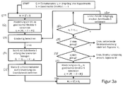
- step S5 of FIG. 2 based on FIG. 3a closer, which, how FIG. 3a are arranged in a loop, so that the adaptation of the adaptation of the coupling matrix M i can be carried out iteratively.
- a first similarity transformation matrix Q 1 a structure matrix S, which maps the predetermined desired physical structure of the filter, and the original and to be formed coupling matrix L are transferred.
- the first coupling matrix M i is consequently the first (modification of) the coupling matrix M 1 .
- the matrix decomposition can also be carried out differently. For example.
- the first similarity transformation matrix Q 1 can also be calculated to have the eigenvectors of the original coupling matrix L.
- the decomposition has the advantage that a subsequent minimization of a structure value deviation ⁇ i of the coupling matrix M takes place on the basis of a change in the similarity transformation matrix Q i .
- the original coupling matrix L created in step S4 is not changed.
- the similarity transformation matrix Q i is shaped in such a way that the scattering parameter data is not changed during the minimization of the structural deviation ⁇ i .
- the computational effort can thus be reduced considerably, the generation of a multiplicity of local minima can be prevented, and at the same time very accurate results can be achieved in the mapping of the physical structure of the filter F.
- S is the (structure) matrix representing the desired physical structure of the filter F.
- This matrix S contains "0" elements at the points where the elements of the matrix M should disappear.
- the remaining elements contain "1".
- the product shown is an elemental product and the equation (2) shown above gives a scalar, the structural deviation ⁇ i , which indicates the deviation of the current coupling matrix M i from the structure S to be achieved.
- the structural deviation ⁇ i should be minimized in the further passage of step S5.
- Equation (3) requires, in addition to the current similarity transformation matrix Q i, a matrix f.
- the matrix f contains the elements f m, n , which are to be calculated according to equation (4).
- the equation (4) for calculating f m, n is accordingly performed as many times as the number of elements of the matrix f. For example, for an N * N matrix, this would be N 2 times.
- the matrix V of Equation (5) represents an auxiliary variable, which is conveniently given with V instead of V i sake.
- L is the original coupling matrix and in equation (4) the current matrix M i is given M for the sake of simplicity.
- S is the (structure) matrix of the physical filter structure to be achieved.
- the matrix J m, n is constructed such that all but the m, n element which is "1", all other elements are "0".
- step S53 thus provides a statement as to which direction the similarity transformation matrix Q i should be adapted. Based on this information, a change in the similarity transformation matrix Q i is then performed in step S54.
- Step S54 of FIG. 3 if i has been incremented by the value "1" before step S54, the fit is based on a previously valid similarity transformation matrix Q i-1 . In the first pass and based on the example according to FIG. 3 For example, the similarity transformation matrix Q i-1 would be the one at the start of step S5 given / inputted unit matrix I.
- ⁇ is a step size which may also be predetermined. However, a user can also enter a value for the step size manually.
- the value of the step size can preferably be chosen / set arbitrarily at the start of step S5 or S54.
- Step S54 may be followed by step S55, which performs orthonormalization of the similarity transformation matrix Q i , which may be necessary and / or advantageous after the adaptation of these in step S54 in order to increase the accuracy of the method according to step S5.
- the Gram-Schmidt method is applied in step S55.
- a query that serves to determine whether the method has already yielded a satisfactory minimization result for the structural deviation ⁇ or whether further runs are necessary.
- it is checked in a first query in step S58 whether the just-determined structural deviation ⁇ i , the current one, is small enough. This is preferably done by means of a comparison between the current Structure deviation ⁇ i and a predetermined limit ⁇ limit . If the current structural deviation ⁇ i is below, then it can be established that the desired structure of the coupling matrix has been reached and the method according to step S5 can be ended.
- a test step S59 queries whether the (current) step size ⁇ has been selected to be small enough. Also a comparison with a threshold value ⁇ boundary is preferably used. If the increment ⁇ is smaller than the limit ⁇ limit , a local minimum has been reached and the remaining structural deviation can be retained. The process of step S5 may be terminated.
- step S510 follows, with which a previously valid value of the structural deviation ⁇ i-1 is compared with the current value ⁇ i .
- FIG. 3 shows here by way of example the comparison of ⁇ 2 with ⁇ 1 .
- the step size ⁇ can be reduced in accordance with step S511.
- a user arbitrarily specifies how the reduction is to take place.
- the calculation rule for the reduction can also be pre-stored and the reduction can thus be carried out automatically.
- step S511 may include resetting the similarity transformation matrix; namely to the previously valid index "i-1", ie the last performed step S54 can be reversed. Subsequently, a newly modified similarity transformation matrix Q i can then be calculated by means of the reduced step size ⁇ in step S 54.
- step S510 is followed by another run starting with step S53, where "i" after the recalculation of the gradient in step S53 by the value "1" can be increased.
- step size can be constant be maintained, if an adjustment according to step S511 should not be considered necessary.
- FIG. 3b a modification of the method according to step S5, wherein the modification is in particular that the index "i" is increased at another time or at another point in the process. That's how it shows FIG. 3b in that the index "i" is already increased before the calculation of the gradient, ie before step S53, and after the tests according to steps S58-S510. Accordingly, the indices of the equations used were adjusted as FIG. 3b also shows.
- the step S5 with its sub-steps described above can preferably be executed by a device designed for this purpose, for example a computer 1 and / or a computer program product.
- the computer 1 may for this purpose have means that can perform the corresponding data processing 1c.
- These means 1c are preferably calculation modules which can perform the data processing in an automated manner in accordance with steps S2-S5.
- a tuning robot 7 or the like To the computer 1, a tuning robot 7 or the like. Be connected, which carries out the tuning of the filter F based on the adapted coupling matrix M.
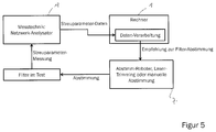
- FIG. 5 shows an exemplary system with measurement technique for measuring the filter F, eg a network analyzer A. The measurement technique can automatically transmit the detected scatter parameter data to the computer 1, which is adapted to the steps S2-S4.
- the computer 1 can, for example, execute the steps S2-S4 immediately after receipt of the measured data.
- the computer 1 can then passed on to a connected with signal and / or data line to the computer 1 tuning means 7 a recommendation for tuning the filter F.
- This recommendation includes at least the adapted coupling matrix M as a result of step S5.
- the tuning means 7 eg a tuning robot or a laser trimming device
- the filter F is then tuned and then re-measured, such as FIG. 5 further shows.
- the in FIG. 5 The process within the voting system shown by the arrows can be iterative. It can also be provided that after the first pass of the loop according to FIG. 5 is canceled.
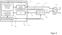
- FIG. 4 An application example of the method described here or the corresponding device / system is of FIG. 4 demonstrated. That's how it shows FIG. 4 the use of an adaptive filter F in a multifunctional radio system in which built-in electrical or mechanical tuning elements are automatically adjusted in quasi-real-time to the requirements of the application.
- a frequency agile transceiver module 1a has a means 1b which can transmit test waveforms via an optional transmission amplifier 8 to a transceiver switch 2. This is done according to FIG. 4 via a first data connection 4.
- Data / signals received by the transmission / reception switch 2 can be received by the transmission / reception module 1a via a second data connection 5.
- the means 1b is further adapted to determine the amplitude and phase of the received signals at a plurality of frequency points and to pass this information to a data processing means 1c.
- the data processing means 1c carries out the steps according to the method described here, in particular S2-S5, preferably S5, and adjusts the adaptive filter F via a third data connection 6, in particular according to the results of step S5.
- a feedback path 3 between the first data connection 4 can be provided switchable, preferably between a position before (in the signal flow direction) the transmitting amplifier 8 and before (in the signal flow direction) the adaptive filter F runs.
- Another application of the methods / devices described herein allows e.g. a vote of a filter F for its production, especially with reduced time and thus higher productivity.
- the device and the computer program product eliminates the expense of prior training of a specialized algorithm (e.g., neural network). Lossy filters can be tuned.
- a parameter set with an arbitrary structure can be reshaped so that it is comparable to the physical structure of the filter. This allows more robust and faster method of parameter extraction.
Landscapes
- Engineering & Computer Science (AREA)
- Computer Networks & Wireless Communication (AREA)
- Signal Processing (AREA)
- Computer Hardware Design (AREA)
- Microelectronics & Electronic Packaging (AREA)
- Complex Calculations (AREA)
Abstract
Description
- Die vorliegende Anmeldung betrifft eine Vorrichtung zum Abstimmen (Tunen) von Filtern und entsprechende Verfahren. Insbesondere beschreibt die vorliegende Anmeldung ein Verfahren, mit dem eine Koppelmatrix mit weniger Zeit- und Rechenaufwand erstellt werden kann. Die so erstellte Koppelmatrix kann die physikalische Struktur eines abzustimmenden Filters sehr genau wiedergeben.
- Viele kommerziell eingesetzte Resonator-Filter, u.a. Hohlleiterfilter, müssen nach der Fertigung oder im Betrieb, wie z.B. Adaptive Filter für Kognitive-Radio-Anwendungen, abgestimmt werden, damit sie die vorgegebenen Spezifikationen erfüllen. Die Aufgabe der Abstimmung (Tuning) besteht in der Einstellung der Kopplungen und Resonanzfrequenzen der Resonatoren. Aufgrund der Komplexität des Zusammenwirkens dieser Parameter ist die Abstimmung schwierig und bislang mit hohem Zeit-/Rechenaufwand verbunden. Bekannte Ansätze zur Abstimmung von Filtern haben insbesondere Nachteile im Hinblick auf den Aufwand, der für die Abstimmung oder die Vorbereitung der Abstimmungsvorrichtungen notwendig ist, der Konvergenz und/oder der Abbildung der physikalischen Struktur des Filters mittels Koppelmatrizen.
- Es existieren Ansätze für das Abstimmen bzw. den Abgleich von Filtern, die auf neuralen Netzen basieren, die auf die abzugleichende Struktur trainiert wurden. Beispielsweise beschreibt J. J. Michalski "Artificial Neural Networks Approach in Microwave Filter Tuning", Progress In Electromagnetics Research M, Vol. 13, 2010 einen solchen Ansatz. Die so vorab trainierten Vorrichtungen bzw. neuronalen Netze sind dann allerdings nur für die trainierte Struktur anwendbar, so dass deren Flexibilität im Hinblick auf verschiedene Filterstrukturen stark eingeschränkt ist oder sogar keine Flexibilität vorhanden ist. Ferner wäre es wünschenswert, den Aufwand für die vorab durchzuführenden Trainings einsparen zu können.
- Ferner sind Verfahren zur Abstimmung von Filtern bekannt, die den Ansatz einer Parameterextraktion aus Messdaten verwenden, wie z.B.
US 2006/202775 A1 undUS 2009/121802 A1 . Die dabei verwendeten Optimierungsverfahren haben jedoch Nachteile im Hinblick auf ihre Konvergenzeigenschaft. Amari et al. beschreiben die bekannten Parameterextraxtionen als schwierig handhabbar im Hinblick auf deren Konvergenzeigenschaften (S. Amari et. al.: "Adaptive Synthesis and Design of Resonator Filters with Source/Load-Multiresonator Coupling", IEEE Transcations on Microwave theory and techniques, vol. 50, no. 8, August 2002). - Zwar beschreiben V. Miraftab et. al. robustere Verfahren zur Parameterextraktion ("Generalized lossy microwave filter coupling matrix synthesis and design using mixed technologies" in IEEE Transcations on Microwave theory and techniques, vol. 56, no. 12, December 2008), jedoch wird bei diesen Verfahren ein Parametersatz erzeugt, der in seiner Struktur nicht dem physikalischen Aufbau des Filters entspricht bzw. diesen nicht abbildet. Dieser Ansatz kann deshalb alleine nicht für die Filter-Abstimmung herangezogen sein.
- Es besteht Bedarf für ein Verfahren zur Erstellung einer Koppelmatrix, die für die Abstimmung eines Filters herangezogen werden kann, sowie ein Verfahren, eine entsprechende Vorrichtung und ein entsprechendes Computerprogrammprodukt zur Abstimmung eines Filters basierend auf dieser Koppelmatrix. Das Verfahren sollte gute Konvergenzeigenschaften aufweisen, weniger Rechen- und Zeitaufwand erfordern und eine Koppelmatrix erstellen können, die die physikalische Struktur des Filters möglichst genau abbildet. Im Hinblick auf den Rechen- und Zeitaufwand wäre es insbesondere von Vorteil, wenn das Verfahren kein Training für vorbestimmte Filter benötigt, da dann auch eine bessere Flexibilität im Hinblick auf das Abstimmen verschiedener Filter gegeben ist.
- Diese Aufgabe wird von den hier beschriebenen Verfahren gemäß den Ansprüchen 1 und 13, sowie dem Vorrichtungsanspruch 14 und dem Computerprogrammanspruch 15 gelöst. Bevorzugte Weiterentwicklungen werden von den abhängigen Ansprüchen 2-12 beschrieben.
- Gemäß einem Aspekt wird hier ein Verfahren zum Erstellen einer angepassten Koppelmatrix eines Filters bzw. zum Abbilden einer physikalischen Struktur eines Filters beschrieben. Das Verfahren kann die Schritte umfassen: Messen von Streuparameterdaten des Filters, Approximation der gemessenen Streuparameterdaten mittels rationaler Funktionen, Erstellen einer ursprünglichen Koppelmatrix basierend auf den rationalen Funktionen und Erstellen einer angepassten Koppelmatrix, die die physikalische Struktur des Filters abbildet, basierend auf der ursprünglichen Koppelmatrix. Der letzte Schritt kann auch als ein Anpassen/Rekonfigurieren der anzupassenden Koppelmatrix auf die physikalische Struktur des Filters bezeichnet werden (die anzupassende Koppelmatrix kann dabei ausgehend von der ursprünglichen Koppelmatrix iterativ angepasst bzw. erstellt werden).
- Das Messen der Streuparameterdaten kann umfassen, dass ein abzustimmender (zu "tune"-ender) Filter mittels eines Netzwerkanalysators vermessen wird. Die Streuparameterdaten können besonders bevorzugt als Funktion der Frequenz gemessen werden. Die Streuparameterdaten können beispielsweise die Messwerte eines Zweitor umfassen; aber auch komplexere Schaltungen wiedergeben.
- Ein Beispiel für den Schritt der Approximation kann umfassen, dass die Streuparameter beispielsweise in Y-Parameter transformiert werden und diese dann beispielsweise mittels des Verfahrens "vector fitting" weiterverarbeitet werden (das "vector fitting" wird bspw. beschrieben von B. Gustavsen und A. Semlyen, "Rational approximation of frequency domain responses by vector fitting", IEEE Trans. Power Del., vol. 14, no. 3, 1999). Andere Algorithmen bzw. Verfahren können ebenfalls herangezogen werden.
- Der Approximation kann zur weiteren Erhöhung der Zuverlässigkeit und Genauigkeit des Verfahrens ein optionaler Schritt "Deembedding der Messdaten" vorgeschaltet werden. Das "Deembeding" wird besonders bevorzugt, wenn die Approximation auf einem Model rationaler Funktionen geringer Ordnung (z.B. kleiner N) durchgeführt wird, da diese Modelle Zeitverzögerungen an den Filtertoren nicht (nicht genau genug) abbilden können; wobei anzumerken ist, dass die Ordnung des rationalen Modells gleich der Ordnung des realen Filters sein sollte, um ein physikalisch sinnvolles Modell zu erhalten. Bei einem Modell mit rationalen Funktionen geringer Ordnung kann mittels des "Deembedings" möglicher Zeitverzögerungen eine Verbesserung der Genauigkeit der Abbildung erreicht werden. Bevorzugt wird das "Deembedding" mit bekannten Verfahren durchgeführt.
- Das Erstellen der (ursprünglichen) Koppelmatrix (die im Allgemeinen die physikalische Struktur des vermessenen Filters noch nicht abbildet/wiedergibt) aus den rationalen Funktionen kann auf unterschiedliche Weise erfolgen. Ein bevorzugtes Beispiel für die Erstellung der Koppelmatrix wird beispielsweise von V. Miraftab und M. Yu "Advanced Coupling Matrix and Admittance Function Synthesis Techniques for Dissipative Microwave Filters" in IEEE TRANSACTIONS ON MICROWAVE THEORY AND TECHNIQUES, VOL. 57, NO. 10, pp. 2429-2438 (Oktober 2009) beschrieben. Das Ergebnis ist eine vollständig besetzte Koppelmatrix mit komplexen Werten. Die Realteile der Werte beschreiben dabei kapazitive und induktive Kopplungen der Resonatoren des Filters, genauso wie Selbstkopplungseffekte. Imaginäre Teile der Diagonalelemente beschreiben hingegen Verluste innerhalb der Resonatoren. Jedoch sei an dieser Stelle noch einmal darauf hingewiesen, dass die bis dato erzeugte Koppelmatrix noch nicht die reale Topologie des Filters wiedergibt und deshalb in dieser Hinsicht gemäß dem hier beschriebenen Verfahren noch angepasst bzw. rekonfiguriert wird. Mit anderen Worten erfolgt verfahrensgemäß zunächst der Schritt der Erstellung einer ursprünglichen Koppelmatrix, der dann der Schritt des Anpassens auf die Topologie des vermessenen Filters folgt. Bei der Rekonfiguration bzw. bei der Erstellung der angepassten Koppelmatrix werden die Koppelmatrixwerte der ursprünglichen Koppelmatrix mit den gemessenen Werten korreliert.
- Es sei noch einmal festgehalten, dass der Schritt des Erstellens einer Koppelmatrix aus den rationalen Funktionen zunächst eine ursprüngliche Koppelmatrix, nachfolgend mit "L" gekennzeichnet, liefert. Der nachfolgende Schritt der Erstellung bzw. Rekonfiguration bzw. Anpassung liefert dann eine angepasste Koppelmatrix, mit "M" gekennzeichnet, die die physikalische Struktur des Filters wiederspiegelt.
- Die angepasste Koppelmatrix wird während der Anpassung/Rekonfiguration verändert, die ursprünglich erstellte Koppelmatrix hingegen nicht. Das Ergebnis des hier beschriebenen Verfahrens ist die angepasste Koppelmatrix ("M"), deren (anfängliche) Strukturabweichung von einer vorgegebenen Struktur iterativ minimiert werden kann.
- Die verfahrensgemäße Rekonfiguration bzw. Anpassung der ursprünglichen Koppelmatrix ermöglicht es, dass die physikalische Struktur des Filters sehr genau und mit weniger Zeit- und Rechenaufwand nachgebildet werden kann. Es wird eine gute Konvergenz erreicht. Mit anderen Worten umfasst das hier beschriebene Verfahren die Vorteile, dass die Topologie des Filters sehr genau abgebildet werden kann und eine hohe Konvergenz erreicht wird. Im Übrigen wird der Zeit- und Rechenaufwand für die Anpassung der Koppelmatrix auch dadurch reduziert, dass kein Traningsaufwand oder dergleichen anfällt, der z.B. bei Ansätzen mit neuronalen Netzen erforderlich wird.
- Gemäß einem bevorzugten Aspekt kann der Schritt des Erstellens der angepassten Koppelmatrix umfassen, dass eine Strukturabweichung, die eine Abweichung zwischen der angepassten Koppelmatrix (nachfolgend auch nur "Koppelmatrix" im Unterschied zu "ursprüngliche Koppelmatrix") und einer abzubildenden physikalischen Struktur des Filters angibt, iterativ minimiert wird.
- Gemäß einem besonders bevorzugten Aspekt kann eine Strukturmatrix vorgegeben werden, die die abzubildende physikalische Struktur des Filters wiedergeben kann. Die Strukturabweichung kann auf Basis der (angepassten) Koppelmatrix und der Strukturmatrix ermittelt werden. Besonders bevorzugt kann die Strukturabweichung aus einer Differenz zwischen (angepasster) Koppelmatrix und Strukturmatrix ermittelt werden. Bei der Iteration wird dabei ganz besonders bevorzugt für jeden Iterationsdurchlauf eine minimierte Strukturabweichung berechnet, wobei jeweils eine weitere Modifikation der angepassten Koppelmatrix herangezogen wird.
- Mit anderen Worten kann die Strukturabweichung bevorzugt ein Skalar sein, der eine Differenz zwischen der Koppelmatrix und einer Strukturmatrix bzw. einer Koppelmatrix, die mit der Strukturmatrix verrechnet wurde, angibt.
- "Iterative Minimierung" soll besonders bevorzugt umfassen, dass die Strukturabweichung bzw. deren Wert in wiederkehrenden Schleifendurchläufen von Unterschritten der Rekonfiguration minimiert wird - möglichst bevorzugt bis ein globales oder zumindest lokales Minimum gefunden werden konnte.
- Beispielsweise kann die Strukturmatrix eine binäre Matrix sein, das heißt so aufgebaut sein, dass sie ausschließlich "0" und "1" als Elementwerte enthält. Die Strukturmatrix kann bevorzugt die bevorzugte und vorbestimmte Matrixstruktur der Koppelmatrix aufweisen. Dabei weist die Strukturmatrix bevorzugt Elemente mit Wert "0" derart platziert auf, dass an dieser Stelle die Elemente der Koppelmatrix während der Rekonfiguration verschwinden. Mit anderen Worten kann an diesen Stellen der Strukturmatrix eine "1" vorgesehen sein, wo Kopplungen und dgl. der Koppelmatrix erhalten bleiben sollen.
- Die Abweichung zwischen dem gewünschten bzw. zu erreichenden physikalischen Aufbau des Filters und der Koppelmatrix wird von dem Strukturabweichungswert wiedergegeben. Dieser Wert gibt somit an, wie gut die aktuelle (während der Iteration) Koppelmatrix der angestrebten, finalen angepassten Koppelmatrix (als gewünschtes Produkt der Iteration/Rekonfiguration) bereits entspricht.
- Gemäß einem besonders bevorzugten Aspekt kann die Strukturabweichung mittels ε :=|| M - S ∘ M | ermittelt werden. Hier bezeichnet der Operator "○" ein elementweises Produkt (Frobenius-Produkt). Beachtlich ist, dass für die Unterscheidung von aktuellen Werten bzw. aktuellen Matrizen und Werten/Matrizen, die in einem Iterationsdurchlauf vorher oder nachher aktuell sind/waren, ein Index verwendet werden kann. Beispielsweise kann der Index "i" verwendet werden, der bevorzugt eine ganze Zahl aus dem Bereich i = 1, 2, 3, ..., n annehmen kann. Dann kann "i" einen aktuellen Wert oder eine aktuelle Matrix kennzeichnen. Die oben angegebene Gleichung (wie auch die weiteren hier verwendeten Gleichungen) kann entsprechend mit Indizes versehen werden.
- Das vorliegende Verfahren erlaubt es somit, dass ein mit wenig Aufwand auswertbarer Qualitätsparameter, die Strukturabweichung, berechnet werden kann, der die Qualität der Koppelmatrix im Hinblick auf die abzubildenden Topologie des Filters anzeigt und der iterativ minimiert werden kann.
- Gemäß einem bevorzugten Aspekt kann der Schritt des Erstellens der angepassten Koppelmatrix die folgenden Unterschritte umfassen: Ermitteln einer aktuellen Iterationslösung (oder Modifikation) der angepassten Koppelmatrix M basierend auf einer aktuellen (Modifikation der) Ähnlichkeitstransformationsmatrix Q und der ursprünglichen Koppelmatrix, und/oder Ermitteln einer aktuellen Iterationslösung der Strukturabweichung ε.
- Wenn für die aktuellen Werte/Matrizen der Index "i" eingesetzt wird, so wären hier bspw. die Werte Mi, Qi und εi heranzuziehen bzw. zu berechnen. In diesem Fall startete der oben genannte Aspekt besonders bevorzugt von einem Startpunkt mit i = 1. Alle weiteren Berechnungsschritte und/oder (Schleifen-)Durchläufe mit i = 2, 3, 4, etc. der genannten Schritte können sich analog anschließen. Die Koppelmatrix Mi wird während der Iterationen immer weiter modifiziert, um schließlich die gewünschte Minimierung der Strukturabweichung zu erreichen. Konstant und nicht verändert wird hingegen die ursprüngliche Koppelmatrix (bzw. eine matrixzerlegte Untermatrix dieser), die aus den rationalen Funktionen gewonnen wurde und noch nicht die Topologie des Filters wiedergibt.
- Nach jedem Durchlauf der genannten Schritte und bevorzugt nach einer oder jeder Ermittlung der aktuellen Strukturabweichung können ein oder mehrere Prüfschritte vorgesehen sein, die das Erreichen/Erfüllen vorbestimmter Abbruchbedingungen prüfen und ggf. den Abbruch bzw. das Ende der Minimierung festlegen. Weiterhin kann nach jedem Schleifendurchlauf ein Schritt zur Erhöhung von i um den Wert "1" vorgesehen sein. Besonders bevorzugt kann dieser Schritt des Erhöhens von i nach dem Prüfvorgang erfolgen. Zusätzliche Schritte zur Erhöhung von i können optional vorgesehen sein.
- Ein Vorteil des hier beschriebenen Aspektes des Verfahrens ist, dass die ursprüngliche Koppelmatrix so zerlegt wird, dass die Ähnlichkeitstransformationsmatrix gewonnen werden kann, die dann variiert/modifiziert werden kann. Besonders bevorzugt kann die Ähnlichkeitstransformationsmatrix eine Rotationsmatrix sein. Vorbekannte Verfahren hingegen variieren die ursprünglich erstellte Koppelmatrix selbst, was zu unerwünschten Effekten im Hinblick auf die Streuparameter führt, da diese bei einer Änderung der Koppelmatrix selbst verändert werden, so dass sich der Rechen- und Zeitaufwand erhöht und die Konvergenz schlechter wird. So müssen bei den vorbekannten Verfahren vielfältige Randbedingungen an die Streuparameter während der Optimierung eingehalten werden. Dies ist bei dem hier beschriebenen Verfahren, das die Optimierung der Ähnlichkeitstransformationsmatrix vorsieht, vorteilhafterweise nicht notwendig, da die Streuparameter dabei unverändert bleiben.
- Bevorzugt kann die Ähnlichkeitstransformationsmatrix so erstellt werden, dass sie die Eigenschaft aufweist, die gemessenen Streuparameter während der Iteration/Rekonfiguration nicht zu verändern. Mit anderen Worten kann die Anordnung der Filterpole und Nullstellen invariant im Hinblick auf die Modifikation der Ähnlichkeitstransformationsmatrix während der Minimierung der Strukturabweichung sein. Somit kann das hier beschriebene Verfahren besonders vorteilhaft verhindern, dass Streuparameter verändert werden, was u. a. zur Generierung von vielen lokalen Minima führte. Der Aufwand für die Durchführung des Verfahrens kann folglich gesenkt werden und die Konvergenz verbessert werden.
- Gemäß einem bevorzugten Aspekt kann das Ermitteln einer aktuellen (Modifikation der) Ähnlichkeitstransformationsmatrix basierend auf einem Gradienten g der vormals aktuellen Ähnlichkeitstransformationsmatrix und einer vorbestimmten Schrittweite δ durchgeführt werden. Somit kann die Minimierung der Strukturabweichung mit relativ geringem Rechenaufwand mittels eines Gradientenverfahrens durchgeführt werden. Die Verwendung eines Gradientenverfahrens zur Minimierung der Strukturabweichung ist eine besonders bevorzugte Option des hier beschriebenen Verfahrens. Alternative Verfahren zur Minimierung der Strukturabweichung können allerdings auch herangezogen werden, bspw. kann auch ein genetischer Algorithmus für die Minimierung der Strukturabweichung verwendet werden.
- Ganz besonders bevorzugt kann die oben genannte Modifikation der Ähnlichkeitstransformationsmatrix basierend auf einem Gradienten der vormals aktuellen Ähnlichkeitstransformationsmatrix ab einer zweiten Iteration/Durchlauf, d.h. bspw. ab einer Iteration mit i ≥ 2 durchgeführt werden. Mit anderen Worten können die zweite und nachfolgende (Modifikation(en) der) Ähnlichkeitstransformationsmatrizen derart berechnet werden. Für i = 1, d.h. für eine erste Ähnlichkeitstransformationsmatrix, kann bevorzugt ein Startwert vorgegeben werden, d.h. die erste Ähnlichkeitstransformationsmatrix kann abweichend von der unten genannten Gleichung gewonnen werden, z.B. durch eine Matrixzerlegung von L.
- Indizes für den Gradienten und die Ähnlichkeitstransformationsmatrizen werden in der unten folgenden Gleichung nicht angegeben, diese können entsprechend der Erhöhung des Iterationsindexes "i" eingesetzt werden. Die neue aktuelle bzw. weitere Modifikation der Ähnlichkeitstransformationsmatrix kann insbesondere so berechnet werden, dass die zuvor gültige Ähnlichkeitstransformationsmatrix und der Gradient dieser zuvor gültigen Ähnlichkeitstransformationsmatrix für die Berechnung heranzogen werden. Somit kann die neue aktuelle Modifikation der Ähnlichkeitstransformationsmatrix besonders bevorzugt mittels der Gleichung Q i := Q - δ · g ermittelt werden.
- Bevorzugt kann der Parameter δ frei wählbar sein und eine Schrittweite angeben, die bestimmt wie weit bei einem Iterationsdurchlauf in die Richtung des Gradienten gegangen werden soll. Bevorzugt wird ein Startwert für δ bereits beim Start des Anpassens der Koppelmatrix vorbestimmt oder eingegeben. Der Gradient wird bevorzugt für jeden Durchlauf neu berechnet, d.h. es kann jeweils ein Schritt zur Berechnung von g während eines Iterationsdurchlaufes vorgesehen sein, der besonders bevorzugt vor der Berechnung der nächsten Modifikation der Ähnlichkeitstransformationsmatrix angeordnet sein kann. Der Gradient g kann optional und alternativ auch als Konstante über die Iterationen hinweg beibehalten werden, wenn dieser nach dem ersten Durchlauf einmal ermittelt worden war. In diesem Fall müssen die betroffenen Gleichungen so angepasst werden, dass eine Konstante für den Gradienten eingesetzt wird. Der konstante Gradient g gemäß der oben genannten optionalen Alternative kann besonders bevorzugt während der Optimierung solange verwendet werden, wie Schritte in Richtung des Gradienten noch zu einer kleineren Strukturabweichung führen. Wenn diese Bedingung nicht mehr erfüllt ist, sollte der Gradient angepasst bzw. neu bestimmt werden.
- Die Berechnung des Gradienten gi erfolgt bevorzugt wie folgt:

- Hier ist beachtlich, dass der Index "i" eingesetzt wurde und kennzeichnet, dass die jeweils aktuellen Werte/Matrizen einzusetzen sind. Ferner bezeichnet fm,n die einzelnen Elemente der Matrix f sind. Somit muss der Unterschritt zur Berechnung von fm,n entsprechend häufig der Anzahl der Elemente von f durchgeführt werden. Bei einer N*N-Matrix z.B. N2-mal. Die Matrix V ist eine Hilfsgröße. L ist die ursprüngliche Koppelmatrix. S ist die Matrix der zu erreichenden physikalischen Filterstruktur. Die Matrix Jm,n ist so aufgebaut, dass außer dem m,n-Element, das "1" ist, alle weiteren Elemente "0" sind.
- Das oben beschriebene Berechnen eines Gradienten und einer Minimierung der Strukturabweichung basierend auf dem Gradientenverfahren machen es möglich, dass sehr "feinfühlig" nach einem Minimum gesucht werden kann, ohne dass dazu ein großer Rechenaufwand notwendig wäre.
- Gemäß einem bevorzugten Aspekt kann das Verfahren weiter umfassen: Vergleichen der aktuellen Iterationslösung der Strukturabweichung ε mit einem vorbestimmten Grenzwert εGrenz, und/oder Vergleichen der (aktuellen) Schrittweite δ mit einem vorbestimmten Grenzwert δGrenz.
- Die obigen Vergleichsschritte können bereits bei i = 1 erfolgen, bevorzugt direkt nach dem Schritt des Ermittelns der aktuellen Strukturabweichung. Die erste Prüfung kann allerdings auch erst erstmals bei i > 1, z.B. i = 2, durchgeführt werden, um zu prüfen, ob die Anpassung der Matrix abgeschlossen werden kann.
- Ein vorbestimmter Grenzwert kann beliebig vorgegeben werden. Bevorzugt werden allerdings sehr kleine Werte gesetzt, um eine möglichst hohe Genauigkeit zu gewährleisten. Werte von εGrenz < 10-5 werden bevorzugt, noch bevorzugter wird εGrenz < 10-10 gesetzt und ganz besonders bevorzugt wird εGrenz ≤ 10-12 gesetzt.
- Das Vergleichen der Schrittweite für den aktuellen Iterationsdurchlauf mit einem vorbestimmten Grenzwert δGrenz kann bevorzugt nach jedem Anpassen der Ähnlichkeitstransformationsmatrix bzw. jeder Berechnung der Koppelmatrix M erfolgen. Der Grenzwert für die Schrittweite ist bevorzugt δGrenz < 10-1, noch bevorzugter wird δGrenz < 10-4 gesetzt. Ganz besonders bevorzugt wird δGrenz ≤ 10-5 gesetzt.
- Der Vorteil des Prüfens der Schrittweite liegt darin, dass lokale Minima identifiziert werden können. So kann die Minimierung der Strukturabweichung auf zumindest zwei unterschiedliche Bedingungen hin beendet werden. Einerseits kann die Minimierung beendet werden, wenn der aktuelle Wert für ε den Grenzwert εGrenz unterschreitet. Zusätzlich oder bevorzugt alternativ kann die Minimierung beendet werden, wenn die aktuelle Schrittweite kleiner ist als δGrenz. Im letzten Fall wird sicher und zuverlässig festgestellt, dass ein lokales Minimum gefunden wurde.
- Weiterhin kann das Verfahren ein Abfragen umfassen, ob die aktuelle Strukturabweichung größer ist als die des vorangegangenen Iterationsschrittes, besonders bevorzugt wenn die Strukturabweichung größer als der vorbestimmter Grenzwert ist und/oder die Schrittweite δ größer ist als der vorbestimmte Grenzwert. Ganz besonders bevorzugt werden die beiden Strukturabweichungen des aktuellen und vorangegangenen Durchlaufes miteinander verglichen, wenn sowohl die Strukturabweichung größer als der vorbestimmter Grenzwert ist als auch die Schrittweite δ größer ist als der vorbestimmte Grenzwert. Diese weitere Prüfabfrage kann sicherstellen, dass auch tatsächlich eine Minimierung stattfindet.
- Wird bei diesem Abfrageschritt festgestellt, dass der aktuelle Strukturabweichungswert größer als der vorangegangene ist, so kann ein weiterer Unterschritt vorgesehen sein. Dieser kann umfassen, dass "der letzte Schritt rückgängig gemacht" wird, was insbesondere umfassen kann, dass die (letzte, vorangegangene) Anpassung/Modifikation der Ähnlichkeitstransformationsmatrix rückgängig gemacht wird. Bspw. kann dies bedeuten, dass die Ähnlichkeitstransformationsmatrix wieder auf den zuvor gültigen Stand zurückgesetzt wird oder dass die aktuelle Modifikation der Ähnlichkeitstransformationsmatrix mit neuer Schrittweite neu berechnet wird. Besonders bevorzugt kann gleichzeitig mit dem Zurücksetzen der Ähnlichkeitstransformationsmatrix auch die Schrittweite δ angepasst und besonders bevorzugt verkleinert werden. Beispielsweise kann die Schrittweite δ automatisiert verkleinert werden. Es kann bspw. vorgesehen sein, dass die Schrittweite δ automatisch halbiert, um eine Zehnerpotenz reduziert oder auf eine andere Art und Weise verändert wird. Ein manuelles Anpassen kann allerdings auch vorgesehen sein.
- Mit anderen Worten kann das Verfahren ein Zurücksetzen der Ähnlichkeitstransformationsmatrix auf den vorangegangenen Iterationsschritt und Verkleinern der Schrittweite δ umfassen, wenn die aktuelle/letzte Strukturabweichung größer ist als die des vorangegangenen Iterationsschrittes. Dies erlaubt es sicherzustellen, dass die Minimierung nicht in die "falsche Richtung" läuft und tatsächlich eine Minimierung der Strukturabweichung erfolgt. Die Sicherheit des Verfahrens im Hinblick auf die Ergebniszuverlässigkeit und die Konvergenz werden somit weiter erhöht.
- Bei Verwendung von Indizes zur Unterscheidung der Iterationen kann nach dem Ende der Prüfschritte oder vor dem Start der Berechnung von einer weiteren Iterationslösung der Koppelmatrix besonders bevorzugt ein Schritt vorgesehen sein, der den Indexwert um den Wert "1" erhöht. Zusätzlich oder alternativ können weitere Schritte zur Erhöhung vorgesehen sein. Gemäß einem besonders bevorzugten Aspekt kann ein einzelner Schritt zur Erhöhung des Indexes i um den Wert "1" vor dem Berechnen des neuen Gradienten in einem Durchlauf ab i = 2 vorgesehen sein.
- Gemäß einem bevorzugten Aspekt kann die Iteration beendet werden, wenn eine (aktuelle) Strukturabweichung kleiner als der vorbestimmte Grenzwert ist und/oder (besonders bevorzugt wird die "oder"-Option), die (aktuelle) Schrittweite δ kleiner als der vorbestimmte Grenzwert ist. Somit wird das Ende der Minimierung sicher feststellbar festgelegt.
- Der Start der Iteration kann gemäß einem bevorzugten Aspekt darauf basieren bzw. die erste Iterationslösung der Koppelmatrix M1 kann mittels einer ersten Ähnlichkeitstransformationsmatrix ermittelt werden, die aus einer Matrixzerlegung der ursprünglichen Koppelmatrix L resultieren kann. Die erste Ähnlichkeitstransformationsmatrix kann die Form

- Dabei ist die Beschreibung der Eingangs- und Ausgangstore des Filters auf die äußersten Zeilen und Spalten verteilt, damit diese bei der Transformation während der Minimierung der Strukturabweichung nicht verändert werden. Die innere Matrix (Submatrix) QINNEN kann wiederrum eine Ähnlichkeitstransformationsmatrix sein. Die oben angegebene Form der Ähnlichkeitstransformationsmatrix kann die allgemeinste Form angeben, mit der das hier vorgestellte Verfahren so durchführbar ist, dass die Streuparameterwerte während der Minimierung nicht geändert werden. Dadurch kann hier vorteilhaft die gute Konvergenz erreicht werden und gleichzeitig verhindert werden, dass das Verfahren zur Anpassung der Koppelmatrix zu komplexen Rechenoperationen führt und ggf. das Ergebnis nicht genau genug werden könnte.
- Die oben angegebene Form der Ähnlichkeitstransformationsmatrix hat zwei bevorzugte Eigenschaften: Die verallgemeinerten Eigenwerte des Matrixbüschels (Matrix pencil) (L, I) bleiben während der Transformation bzw. Matrixzerlegung unverändert. Die Eigenwerte sind gleich den Übertragungspolen des Filters. Diese Eigenschaft wird dadurch erreicht, dass die Ähnlichkeitstransformationsmatrix eine Ähnlichkeitstransformation beschreibt. Ferner bleiben die Übertragungs- und Reflektions"nullen" während der Transformation unverändert. Die Position dieser Nullen wird von den Eigenwerten von entsprechenden Minoren beeinflusst. Diese Eigenschaft wird dadurch erreicht, dass auch die Transformationen der Minore Ähnlichkeitstransformationen sind.
- Die oben genannten Eigenschaften der oben angegebenen Ähnlichkeitstransformationsmatrix ermöglichen, dass Filterpole und Nullen nicht geändert werden, wenn die Minimierung durchgeführt wird.
- Gemäß einem besonders bevorzugten Aspekt kann die Ermittlung der ersten Iterationslösung der Koppelmatrix M1 mittels der Einheitsmatrix I als erste (Start-)Ähnlichkeitstransformationsmatrix Q1 durchgeführt werden. Die Zerlegung der Koppelmatrix L ergibt dann folglich eine N+2 Koppelmatrix und eine Ähnlichkeitstransformation in Form der Einheitsmatrix I als erste Ähnlichkeitstransformationsmatrix Q1 gemäß Mi := Qi TLQi mit i = 1 für den Start der Minimierung, Q1 in diesem Fall als die Einheitsmatrix I und L die umzuformende Koppelmatrix bzw. ursprüngliche Koppelmatrix zum Start der Minimierung.
- Gemäß einem weiteren besonders bevorzugten Aspekt kann die erste Iterationslösung der Koppelmatrix M1 so ermittelt werden, dass die ursprüngliche Koppelmatrix mittels einer verallgemeinerten Eigenwertzerlegung mit dem Matrix-Büschel (L,I) zerlegt wird, so dass die resultierende Transformationsmatrix die oben angegebenen Form

- Die Zerlegung und anschließende Änderung der Ähnlichkeitstransformationsmatrix während der Minimierung der Strukturabweichung hat den Vorteil, dass die Streuparameterwerte während der Minimierung nicht geändert werden.
- Gemäß einem besonders bevorzugten Aspekt kann nach der Modifikation der Ähnlichkeitstransformationsmatrix eine Orthonormalisierung der modifizierten Ähnlichkeitstransformationsmatrix durchgeführt werden. Dieser bevorzugte weitere Schritt kann verhindern, dass kleine Abweichungen der Ähnlichkeitstransformationsmatrix nach deren Anpassung entlang des Gradienten im Schritt zuvor, ausgeglichen werden können. Besonders bevorzugt wird hier beispielsweise das Gram-Schmidt-Verfahren für die Orthonormalisierung der angepassten Ähnlichkeitstransformationsmatrix durchgeführt. Die Genauigkeit des Verfahrens kann somit weiter erhöht werden.
- Gemäß einem besonders bevorzugten Aspekt kann der in den Figuren bezeichnete Schritt S5 die Unterschritte aufweisen (wobei die oben angegeben Gleichungen mit entsprechenden Indizes "i" für die entsprechenden Schritte verwendet werden können): Ermitteln einer ersten Koppelmatrix M1 basierend auf einer vorgegebenen ersten Ähnlichkeitstransformationsmatrix Q1, die die Einheitsmatrix ist, und der ursprünglichen Koppelmatrix aus Schritt S4. Berechnen der ersten Strukturabweichung basierend auf der ersten Koppelmatrix M1. Prüfen (optional), ob die erste Strukturabweichung kleiner ist als ein vorgegebener Grenzwert. Falls nicht, wird ein erster Gradient g1 berechnet und i auf den Wert "2" erhöht. Anschließend wird eine (zweite) Modifikation der Ähnlichkeitstransformationsmatrix Q2 mittels des zuvor berechneten Gradienten und der zuvor gültigen Ähnlichkeitstransformationsmatrix, bei i = 2 ist dies Q1, ermittelt. Optional wird die Modifikation der Ähnlichkeitstransformationsmatrix Q2 orthonormalisiert. Danach wird die weiter geänderte Koppelmatrix Mi (mittels Qi und der ursprünglichen Koppelmatrix) und die weiter geänderte Strukturabweichung εi berechnet und geprüft, ob die weiter geänderte Strukturabweichung εi kleiner als der vorgegebene Grenzwert ist. Wenn dies nicht der Fall ist, wird geprüft, ob die für die Berechnung der Modifikation der Ähnlichkeitstransformationsmatrix herangezogene Schrittweite klein genug war. Falls dies nicht der Fall ist, wird geprüft, ob der aktuelle Wert der Strukturabweichung größer ist als der zuvor gültige Wert. Falls dies der Fall ist, wird die Ähnlichkeitstransformationsmatrix zurückgesetzt und mit verkleinerter Schrittweite neu berechnet. Falls nicht, wird i um den Wert "1" erhöht und ein weiterer geänderter Wert des Gradienten gi ermittelt. Weiterhin wird eine weitere Modifikation der Ähnlichkeitstransformationsmatrix Qi basierend auf gi und Qi-1 (optionalerweise wird Qi auch orthonormalisiert), eine weiter geänderte Koppelmatrix Mi (mittels Qi und der ursprünglichen Koppelmatrix) und eine weiter geänderte Strukturabweichung εi mit i = 3 berechnet. Anschließend werden die vorgenannten drei Prüfschritte wiederholt. Falls ein weiterer Durchlauf notwendig werden sollte, wird i wiederrum um den Wert "1" erhöht und es erfolgt ein Start bei der Neuberechnung des weiter geänderten Gradienten gi mit den nachfolgenden Schritten wie oben beschrieben.
- Es sei angemerkt, dass die Prüfungsschritte auch abweichend vorgesehen sein können, z.B. in einer abweichenden Reihenfolge. Beispielsweise kann zunächst die Schrittweite geprüft werden, bevor die Strukturabweichung mit einem Grenzwert verglichen wird.
- Ein weiterer besonders bevorzugter Aspekt des in den Figuren bezeichneten Schrittes S5 kann die Unterschritte umfassen (wobei die oben angegeben Gleichungen mit entsprechenden Indizes "i" für die entsprechenden Schritte verwendet werden können): Ermitteln einer ersten Koppelmatrix M1 basierend auf einer vorgegebenen ersten Ähnlichkeitstransformationsmatrix Q1, die die Einheitsmatrix ist, und der ursprünglichen Koppelmatrix aus Schritt S4. Berechnen der ersten Strukturabweichung basierend auf der ersten Koppelmatrix M1. und eines ersten Gradienten g1. Anschließend wird eine (zweite) Modifikation der Ähnlichkeitstransformationsmatrix Qi+1=2 mittels des zuvor berechneten Gradienten und der zuvor gültigen Ähnlichkeitstransformationsmatrix Qi ermittelt. Optional wird die Modifikation der Ähnlichkeitstransformationsmatrix Q2 orthonormalisiert. Danach wird die weiter geänderte Koppelmatrix Mi+1 (mittels Qi+1 und der ursprünglichen Koppelmatrix) und die weiter geänderte Strukturabweichung εi+1 berechnet und geprüft, ob die weiter geänderte Strukturabweichung εi+1 kleiner als der vorgegebene Grenzwert ist. Wenn dies nicht der Fall ist, wird geprüft, ob die für die Berechnung der Modifikation der Ähnlichkeitstransformationsmatrix herangezogene Schrittweite klein genug war. Falls dies nicht der Fall ist, wird geprüft, ob der aktuelle Wert der Strukturabweichung größer ist als der zuvor gültige Wert. Falls dies der Fall ist, wird die Ähnlichkeitstransformationsmatrix zurückgesetzt und mit verkleinerter Schrittweite neu berechnet. Falls nicht, wird i um den Wert "1" erhöht und ein weiterer geänderter Wert des Gradienten gi ermittelt. Weiterhin wird eine weitere Modifikation der Ähnlichkeitstransformationsmatrix Qi+1 basierend auf gi und Qi (optionalerweise wird Qi+1 auch orthonormalisiert), eine weiter geänderte Koppelmatrix Mi+1 (mittels Qi+1 und der ursprünglichen Koppelmatrix) und eine weiter geänderte Strukturabweichung εi+1 mit i = 2 berechnet. Anschließend werden die vorgenannten drei Prüfschritte wiederholt. Falls ein weiterer Durchlauf notwendig werden sollte, wird i wiederrum um den Wert "1" erhöht und es erfolgt ein Start bei der Neuberechnung des weiter geänderten Gradienten gi mit den nachfolgenden Schritten wie oben beschrieben.
- Gemäß einem weiteren bevorzugten Aspekt kann hier auch ein Verfahren zum Abstimmen eines Filters vorgesehen sein, das die angepasste Koppelmatrix verwenden kann, um den Filter abzustimmen (zu "tunen"), die mittels eines Verfahrens nach zumindest einem der voranstehenden Aspekte erstellt wurde. Besonders bevorzugt können die oben erläuterten Verfahrensaspekte zum Abstimmen eines Filters folglich in ein Verfahren eingegliedert sein, das die Koppelmatrix nach der Abstimmung zum Einstellen/Abstimmen eines Filters heranzieht.
- Gemäß einem weiteren Aspekt kann eine Vorrichtung zum Erstellen einer angepassten Koppelmatrix eines Filters und/oder zum Abstimmen eines Filters mittels einer angepassten Koppelmatrix hier vorgesehen sein. Die Vorrichtung zum Erstellen der angepassten Koppelmatrix kann aufweisen: ein oder mehr Mittel zum Messen von Streuparameterdaten des Filters, ein oder mehr Mittel zum Approximieren der gemessenen Streuparameterdaten mittels rationaler Funktionen, ein oder mehr Mittel zum Erstellen der ursprünglichen Koppelmatrix basierend auf den rationalen Funktionen und/oder zum Erstellen der angepassten Koppelmatrix (die auf die physikalische Struktur des Filters angepasst ist). Die Vorrichtung zum Tunen des Filters kann die Vorrichtung zum Erstellen der angepassten Koppelmatrix und ein oder mehr Mittel zum Abstimmen des Filters basierend auf der angepassten Koppelmatrix aufweisen. Das Mittel zum Abstimmen des Filters kann beispielsweise eine Abstimmschraube oder dgl. sein. Das Abstimmen kann automatisiert oder manuell erfolgen. Das Mittel zum Messen von Streuparameterdaten kann ein Netzwerkanalysator sein. Die Mittel zum Approximieren, Erstellen der Koppelmatrizen können ein oder mehrere Rechner/Computer sein.
- Gemäß einem weiteren Aspekt kann ein Computerprogrammprodukt mit Computerprogrammmitteln hier vorgesehen sein, die auf einem computerlesbaren Medium speicherbar sein können und von einem Computer ausführbar sein können, wobei die Computerprogrammmittel ausführbare Anweisungen enthalten können, die den Computer dazu veranlassen können, die Schritte gemäß zumindest einem der vorstehend genannten Verfahrensaspekte auszuführen.
- Zusammenfassend wird hier ein Verfahren vorgestellt, das eine gute Konvergenz aufweist, weniger Rechenaufwand erzeugt und die physikalische Struktur des Filters, der abzustimmen ist, mittels einer angepassten Koppelmatrix sehr genau wiedergeben kann. Weiterhin werden eine entsprechende Vorrichtung zum Durchführen des Verfahrens zum Abstimmen des Filters und/oder zum Anpassen der Koppelmatrix und ein entsprechendes Computerprogrammprodukt beschrieben.
- Gegenüber reiner Optimierung oder Abstimmung von Hand kann somit mittels der hier beschriebenen Verfahren(s), der Vorrichtung(en) und den entsprechenden Computerprogrammprodukten eine höhere Zuverlässigkeit und Geschwindigkeit des Verfahrens erreicht werden. Dies ermöglicht die Verwendung entsprechender adaptiver Filter in multifunktionalen und/oder kognitiven Funksystemen, in denen eingebaute elektrische oder mechanische Abstimmelemente automatisch in quasi-Echtzeit den Anforderungen der Anwendung angepasst werden. In Anwendungen der Filterabstimmung kann nach der Fertigung durch reduzierten Zeitbedarf eine höhere Produktivität erreicht werden. Durch die allgemeine Einsetzbarkeit des Verfahrens fällt der Aufwand für vorheriges Training eines spezialisierten Algorithmus (wie z.B. bei neuronalen Netzen) weg. Das Verfahren ist auch für verlustbehaftete Filter einsetzbar.
- Das hier dargelegte Verfahren und die dazugehörige Vorrichtung/Computerprogrammprodukt werden im Folgenden exemplarisch mit Bezug auf die beigefügten, schematischen Zeichnungen beschrieben. Es zeigen
- Fig. 1
- die beispielhafte Struktur eines Filter mit drei Resonatoren und einem Eingangs- und Ausgangstor (
Fig. 1a ), sowie eine Darstellung des Strukturgraphen ausFig. 1a als Parametersatz in Form einer Matrix (Fig. 1b ), - Fig. 2
- ein Verfahren zur Abstimmung eines Filters,
- Fig. 3a
- ein Verfahren zur Rekonfiguration einer Koppelmatrix während eines Abstimmungsverfahrens,
- Fig. 3b
- ein Verfahren zur Rekonfiguration einer Koppelmatrix während eines Abstimmungsverfahrens, und
- Figs. 4 und 5
- Anwendungsbeispiele eines Abstimmungsverfahrens.
- Im Folgenden werden verschiedene Beispiele detailliert und unter Bezugnahme auf die Figuren beschrieben. Gleiche bzw. ähnliche Elemente in den Figuren werden hierbei mit gleichen Bezugszeichen bezeichnet. Die vorliegende Vorrichtung und die Verfahren sind jedoch nicht auf die beschriebenen Kombinationen von Merkmalen begrenzt. Vielmehr sollen auch weitere Modifikationen und Kombinationen von Merkmalen verschiedener Beispiele im Rahmen des Schutzumfangs der unabhängigen Ansprüche umfasst sein.
-
Fig. 1a zeigt zunächst allgemein die Struktur eines Filters F, beispielhaft mit drei Resonatoren (Knoten 1, 2 und 3). Diese Resonatoren sind untereinander mit der Koppelstärke cxy verkoppelt (eingezeichnete Kanten). Der Filter F ist über die Ein- und Ausgangstore (Knoten S=Quelle und L=Last) mit der Umgebung verbunden. - Der Strukturgraph lässt sich äquivalent als Parametersatz in Form einer Matrix darstellen, die sog. Koppelmatrix L.
Figur 1b zeigt eine Koppelmatrix L, die den Strukturgraph derFigur 1a entsprechend abbildet. Die Diagonaleinträge f1 bis f3 beschreiben hier eine mögliche Abweichung der Resonanzfrequenz des Resonators von der Mittenfrequenz. Die Einträge können auch gleich "0" sein. Weiterhin ist ersichtlich, dass die entsprechenden Kopplungen bzw. Koppelstärken cxy derFigur 1a in der Matrix elementweise eingetragen sind. -
Figur 2 zeigt nun beispielhaft eine Abfolge von Schritten bzw. einen Prozess zur Abstimmung eines Filters F. Dieses Verfahren enthält zudem ein Verfahren zur Erstellung einer Koppelmatrix M, die die Topologie des Filters F wiederspiegelt. Zunächst werden hier zum Start des Verfahrens, das bevorzugt als eine Schleife aufgebaut sein kann, die Streuparameterdaten gemessen (Schritt S1). Beispielsweise kann dazu ein Netzwerkanalysator A (s.Figur 5 ) herangezogen werden, mit dem der abzustimmende Filter F vermessen wird. - Anschließend werden die gemessenen Streuparameterdaten in eine Vorrichtung zur Datenverarbeitung, bspw. einen Rechner 1 (s.
Figur 5 ), eingegeben. Dies kann über eine Datenleitung oder Funkverbindung erfolgen oder auch manuell, z.B. mittels Transport und Überspielen auf/von einem Speichermittel. Die Datenverarbeitung umfasst dann, wie beispielhaft inFigur 2 gezeigt wird, zunächst einen Schritt S2, der als "Deembedding" der Messdaten bezeichnet wird. Die gemessenen Streuparameterdaten können Zeitverzögerungen enthalten, die von einer Zeitverzögerungen an den Toren des Filters stammen können. Mittels "Deembedding" können diese Zeitverzögerungen entfernt werden. Das "Deembedding" kann mittels bekannter Verfahren durchgeführt werden und erfolgt bevorzugt in den Fällen, in denen Modelle rationaler Funktionen mit niedriger Ordnung in Schritt S3 herangezogen werden, da diese Modelle Zeitverzögerungen nicht zuverlässig abbilden können. - In einem weiteren Schritt S3 erfolgt dann die bereits angesprochene Abbildung bzw. Approximation der Streuparameterdaten mittels rationaler Funktionen. Beispielsweise können für die Beschreibung der Messdaten mittels rationaler Funktionen zunächst Y-Parameter aus den Streuparameterdaten gewonnen werden, aus denen dann mittels rationaler Approximation die rationalen Funktionen ermittelt werden können. Ein vorbekannter und bevorzugt in Schritt S3 verwendeter Algorithmus für die rationale Approximation ist der "Vektor Fitting Algorithm" (bspw. B. Gustavsen und A. Semlyen, "Rational approximation of frequency domain responses by vector fitting", IEEE Trans. Power Del., vol. 14, no. 3, 1999). Andere Algorithmen bzw. Verfahren können ebenfalls herangezogen werden.
- Nachdem die rationalen Funktionen aufgestellt wurden, wird der Schritt S4 ausgeführt, der eine Umrechnung des rationalen Modells/Funktionen in eine ursprüngliche Koppelmatrix L vorsieht. Diese Umrechnung bzw. die Extraktion der ursprünglichen Koppelmatrix L kann bevorzugt mittels dem von V. Miraftab et. al. in "Generalized lossy microwave filter coupling matrix synthesis and design using mixed technologies" in IEEE Transcations on Microwave theory and techniques, vol. 56, no. 12, December 2008 beschriebenen Verfahren erfolgen. Andere Algorithmen bzw. Verfahren können auch herangezogen werden.
- Das Ergebnis des Schrittes S4 ist somit die ursprüngliche Koppelmatrix L, die jedoch noch nicht die physikalische Struktur des abzustimmenden Filters wiederspiegelt und deshalb noch nicht zum hochgenauen Abstimmen/Einstellen eines Filters geeignet ist. Deshalb schließt sich verfahrensgemäß ein weiterer Schritt S5 an, der eine Anpassung/Rekonfiguration der ursprünglichen Koppelmatrix L vorsieht. Der Schritt S5 ermöglicht es, dass die abzubildende physikalische Filterstruktur sehr genau wiedergegeben werden kann.
- Der Schritt S5 umfasst mehrere Unterschritte, die vor dem Hintergrund der
Figuren 3a und3b unten im Detail erläutert werden sollen. - Nach dem Schritt S5 liegt eine Koppelmatrix M vor, die die physikalische Struktur des abzustimmenden Filters F sehr genau wiederspiegelt, so dass dann im Schritt S6 das Abstimmen des Filters F erfolgen kann. Dies kann automatisiert oder von Hand erfolgen, z.B. können dazu Abstimmschrauben als Abstimmmittel verwendet werden.
- Das Verfahren zur Abstimmung des Filters F sieht nach dem Schritt S6 optional vor, dass die vorbeschriebenen Schritte in einer Schleife so lange weiter durchgeführt werden, bis eine vorbestimmte erwünsche Filter-Charakteristik erreicht worden ist. Es kann allerdings auch bestimmt sein, dass nur ein Durchlauf der Schritte S1-S6 erfolgen soll, insbesondere wenn eine besonders kurze Abstimmdauer priorisiert werden soll.
- Nachfolgend werden nun die Unterschritte des Schrittes S5 der
Figur 2 anhand derFigur 3a näher beleuchtet, die, wieFigur 3a zeigt, in einer Schleife angeordnet sind, so dass die Anpassung des Anpassung der Koppelmatrix Mi iterativ erfolgen kann. Zum Start werden eine erste Ähnlichkeitstransformationsmatrix Q1, eine Strukturmatrix S, die die vorbestimmte gewünschte physikalische Struktur des Filters abbildet, und die ursprüngliche und umzuformende Koppelmatrix L übergeben. In Schritt S51 wird zum Start des Verfahrens gemäß Schritt S5 eine Koppelmatrix Mi mit "i"=1 definiert. Nach dem Start ist die erste Koppelmatrix Mi folglich die erste (Modifikation der) Koppelmatrix M1. Schritt S51 umfasst eine Matrixzerlegung von Lgemäß (1):
- Die Zerlegung im ersten Schritt, bei i=1, erfolgt bevorzugt, und wie das Feld "Start" in
Figur 2 anzeigt, so, dass Q1 die Einheitsmatrix I ist und L die zuvor in Schritt S4 aufgestellte ursprüngliche Koppelmatrix L. Damit entspricht M1 der ursprüngliche Koppelmatrix L. Die Matrixzerlegung kann auch abweichend davon durchgeführt werden. Bspw. kann die erste Ähnlichkeitstransformationsmatrix Q1 auch so berechnet werden, dass sie die Eigenvektoren der ursprünglichen Koppelmatrix L aufweist. - Die Zerlegung bringt den Vorteil mit sich, dass eine nachfolgende Minimierung einer Strukturwertabweichung εi der Koppelmatrix M basierend auf einer Änderung der Ähnlichkeitstransformationsmatrix Qi erfolgt. Die ursprüngliche Koppelmatrix L, die in Schritt S4 erstellt wurde, wird hingegen nicht geändert. Die Ähnlichkeitstransformationsmatrix Qi ist dabei so geformt, dass die Streuparameterdaten während der Minimierung der Strukturabweichung εi nicht geändert werden. Der Rechenaufwand kann folglich erheblich reduziert werden, die Entstehung einer Vielzahl lokaler Minima kann verhindert werden und gleichzeitig können sehr genauen Ergebnissen bei der Abbildung der physikalischen Struktur des Filters F erzielt werden.
- Die genannte Strukturabweichung εi wird erstmals im Schritt S52 ermittelt; und zwar basierend auf der Gleichung (2)

- Die Minimierung der Strukturabweichung εi erfolgt mittels eines Gradientenverfahrens, das in den
Figuren 3a und3b gezeigt ist. Dazu wird zunächst in einem Schritt S53 der aktuelle Gradient gi der aktuellen Ähnlichkeitstransformationsmatrix Qi berechnet. Der Begriff "aktuell" soll insbesondere den Wert eines "aktuellen Iterationsdurchlaufes" des Schrittes S5 bezeichnen bzw. inFigur 3a den Wert mit dem Index "i". Die Berechnung des Gradienten gi erfolgt basierend auf den Gleichungen (3)-(5):
- Die Gleichung (3) benötigt neben der aktuellen Ähnlichkeitstransformationsmatrix Qi eine Matrix f. Die Matrix f enthält die Elemente fm,n, die gemäß Gleichung (4) zu berechnen sind. Die Gleichung (4) zur Berechnung von fm,n wird entsprechend so häufig durchgeführt, wie die Anzahl der Elemente der Matrix f ist. Bei einer N*N-Matrix wäre dies z.B. N2-mal. Die Matrix V der Gleichung (5) stellt eine Hilfsgröße dar, die der Einfachheit halber mit V statt Vi angegeben wird. Ferner ist anzumerken, dass L die ursprüngliche Koppelmatrix ist und in Gleichung (4) die aktuelle Matrix Mi der Einfachheit halber mit M angegeben wird. S ist die (Struktur-)Matrix der zu erreichenden physikalischen Filterstruktur. Die Matrix Jm,n ist so aufgebaut, dass außer dem m,n-Element, das "1" ist, alle weiteren Elemente "0" sind.
- Die Gleichung (3) gemäß Schritt S53 liefert somit eine Aussage darüber, in welche Richtung die Ähnlichkeitstransformationsmatrix Qi angepasst werden soll. Basierend auf dieser Information wird dann im Schritt S54 eine Änderung der Ähnlichkeitstransformationsmatrix Qi durchgeführt. Schritt S54 der
Figur 3 zeigt hier die Anpassung basierend auf einer zuvor gültigen Ähnlichkeitstransformationsmatrix Qi-1, wenn i vor dem Schritt S54 um den Wert "1" erhöht worden ist. Im ersten Durchlauf und basierend auf dem Beispiel gemäßFigur 3 wäre die Ähnlichkeitstransformationsmatrix Qi-1 die beim Start von Schritt S5 übergebene/eingegebene Einheitsmatrix I. Die Gleichung (6) zum Ändern der Ähnlichkeitstransformationsmatrix Qi lautet:
- In Gleichung (6) ist δ eine Schrittweite, die ebenfalls vorgegeben bzw. vorbestimmt sein kann. Ein Anwender kann einen Wert für die Schrittweite jedoch auch manuell eingeben können. Der Wert der Schrittweite kann zum Start von Schritt S5 bzw. S54 bevorzugt beliebig gewählt/gesetzt werden.
- An den Schritt S54 kann sich der Schritt S55 anschließen, der eine Orthonormalisierung der Ähnlichkeitstransformationsmatrix Qi durchführt, die nach der Anpassung dieser in Schritt S54 notwendig und/oder von Vorteil sein kann, um die Genauigkeit des Verfahrens gemäß Schritt S5 zu erhöhen. Bevorzugt wird das Gram-Schmidt-Verfahren im Schritt S55 angewendet.
-
Figur 3a zeigt nun, dass eine zweite Modifikation der Koppelmatrix Mi (i=2) in Schritt S56 berechnet wird, wiederrum basierend auf der ursprünglich erstellten Koppelmatrix L, die für das hier beschriebene Verfahren nicht verändert wird, und basierend auf der zuvor angepassten Ähnlichkeitstransformationsmatrix Qi. Wenn das Verfahren gemäß Schritt S5 mit der Einheitsmatrix I als Matrix Q1 startet, so würde die Koppelmatrix M2 basierend auf der einmal modifizierten Einheitsmatrix I, der Ähnlichkeitstransformationsmatrix Q2, ermittelt. Die Gleichung entspricht dabei der Gleichung (1) aus Schritt S51. Die neu ermittelte Koppelmatrix M2 wird anschließend in Schritt S57 analog zu Schritt S52 herangezogen, um die geänderte Strukturabweichung ε2 zu berechnen, s. dazu die Gleichung (2). - Danach schließt sich gemäß dem beispielhaften Ablauf der
Figur 3a ein Abfragen an, das dazu dient, festzustellen, ob das Verfahren bereits ein befriedigendes Minimierungsergebnis für die Strukturabweichung ε ergeben hat oder ob weitere Durchläufe notwendig sind. Dazu wird in einer ersten Abfrage in Schritt S58 geprüft, ob die soeben ermittelte Strukturabweichung εi, die aktuelle, klein genug ist. Bevorzugt erfolgt dies mittels eines Vergleiches zwischen der aktuellen Strukturabweichung εi und einem vorbestimmten Grenzwert εGrenz. Liegt die aktuelle Strukturabweichung εi darunter, so kann festgestellt werden, dass die gewünschte Struktur der Koppelmatrix erreicht worden ist und das Verfahren gemäß Schritt S5 kann beendet werden. - Andernfalls folgt ein Prüfschritt S59, der abfragt, ob die (aktuelle) Schrittweite δ klein genug gewählt worden war. Auch dazu wird bevorzugt ein Vergleich mit einem Grenzwert δGrenz herangezogen. Ist die Schrittweite δ kleiner als der Grenzwert δGrenz so wurde ein lokales Minimum erreicht und die verbleibende Strukturabweichung kann beibehalten bleiben. Das Verfahren gemäß Schritt S5 kann beendet werden.
- Andernfalls, falls auch Schritt S59 ein negatives Prüfergebnis ergibt, folgt ein Schritt S510, mit dem ein zuvor gültiger Wert der Strukturabweichung εi-1 mit dem aktuellen Wert εi verglichen wird.
Figur 3 zeigt hier beispielhaft den Vergleich von ε2 mit ε1. Ist der aktuelle Wert, hier ε2, größer, so kann gemäß Schritt S511 die Schrittweite δ verkleinert werden. Bevorzugt gibt ein Anwender beliebig vor, wie die Verkleinerung erfolgen soll. Die Rechenvorschrift für die Verkleinerung kann jedoch auch vorgespeichert sein und die Verkleinerung somit automatisiert durchgeführt werden. Weiterhin kann Schritt S511 umfassen, dass die Ähnlichkeitstransformationsmatrix wieder zurückgesetzt wird; und zwar auf die zuvor gültige mit Index "i-1", d.h. der zuletzt durchgeführte Schritt S54 kann rückgängig gemacht werden. Anschließend kann dann eine neu modifizierte Ähnlichkeitstransformationsmatrix Qi mittels der verkleinerten Schrittweite δ in Schritt S54 errechnet werden. - Falls der aktuelle Wert der Strukturabweichung εi jedoch kleiner als der vorangegangene sein sollte, so schließt sich an den Schritt S510 ein weiterer Durchlauf startend mit Schritt S53 an, wobei "i" nach der Neuberechnung des Gradienten in Schritt S53 um den Wert "1" erhöht werden kann.
- Falls der Gradient g der Gradient des ersten Durchlaufes, d.h. g1, konstant bleiben soll, so können weitere Durchläufe mit S54 starten. Die Schrittweite kann konstant beibehalten werden, falls nicht eine Anpassung gemäß Schritt S511 für notwendig erachtet werden sollte.
- Weiterhin zeigt
Figur 3b eine Abwandlung des Verfahrens gemäß Schritt S5, wobei die Abwandlung insbesondere darin besteht, dass der Index "i" zu einem anderen Zeitpunkt bzw. an einer anderen Stelle im Verfahren erhöht wird. So zeigt dieFigur 3b , dass der Index "i" bereits vor der Berechnung des Gradienten, d.h. vor Schritt S53, und nach den Prüfungen gemäß den Schritten S58-S510 erhöht wird. Entsprechend wurden die Indizes der verwendeten Gleichungen angepasst, wieFigur 3b ebenfalls zeigt. - Andere Abwandlungen bzw. Abweichungen von der Abfolge der Schritte je Durchlauf können optional auch möglich sein, solange eine Minimierung der Strukturabweichung εi mittels der Abänderung der Ähnlichkeitstransformationsmatrix Qi, wie beschrieben, erfolgt und der Erfolg dieser Minimierung regelmäßig geprüft wird, z.B. in jedem Iterationsdurchlauf, in jedem zweiten oder dgl. Bei Abwandlungen der Abfolge können Änderungen der Gleichungen, insbesondere im Hinblick auf die verwendeten Indizes, notwendig sein, so wie dies beispielhaft für die Abwandlung gemäß
Figur 3b inFigur 3b vorgeführt wird. - Der Schritt S5 mit seinen oben beschriebenen Unterschritten kann bevorzugt von einer dazu eingerichteten Vorrichtung, z.B. einem Rechner 1 und/oder einem Computerprogrammprodukt ausgeführt werden. Der Rechner 1 kann dazu Mittel aufweisen, die die entsprechende Datenverarbeitung 1c ausführen können. Bevorzugt sind diese Mittel 1c Rechenmodule, die die Datenverarbeitung gemäß Schritten S2-S5 automatisiert durchführen können. An den Rechner 1 kann ein Abstimmroboter 7 oder dgl. angeschlossen sein, der die Abstimmung des Filters F basierend auf der angepassten Koppelmatrix M ausführt.
Figur 5 zeigt ein beispielhaftes System mit Messtechnik zur Vermessung des Filters F, z.B. einem Netzwerkanalysator A. Die Messtechnik kann die erfassten Streuparameterdaten automatisch an den Rechner 1 übermitteln, der dazu eingerichtet ist, die Schritte S2-S4 auszuführen. Der Rechner 1 kann bspw. unmittelbar nach Erhalt der Messdaten die Schritte S2-S4 ausführen. Der Rechner 1 kann danach an ein mit Signal- und/oder Datenleitung an den Rechner 1 angeschlossenes Abstimmmittel 7 eine Empfehlung für die Abstimmung des Filters F weitergegeben. Diese Empfehlung beinhaltet zumindest die anpasste Koppelmatrix M als Ergebnis des Schrittes S5. Mittels des Abstimmmittels 7 (z.B. ein Abstimmroboter oder eine Lasertrimmingeinrichtung) und/oder manuellem Abstimmen wird der Filter F dann abgestimmt und danach neu vermessen, wieFigur 5 weiter zeigt. Der inFigur 5 mittels den Pfeilen gezeigte Ablauf innerhalb des Abstimmsystems kann iterativ erfolgen. Es kann auch vorgesehen sein, dass nach dem ersten Durchlauf der Schleife gemäßFigur 5 abgebrochen wird. - Ein Anwendungsbeispiel des hier beschriebenen Verfahrens bzw. der entsprechenden Vorrichtung/System wird von
Figur 4 aufgezeigt. So zeigt dieFigur 4 die Verwendung eines adaptiven Filters F in einem multifunktionalen Funksystem, in dem eingebaute elektrische oder mechanische Abstimmelemente automatisch in quasi-Echtzeit den Anforderungen der Anwendung angepasst werden. Konkret zeigt dieFigur 4 beispielhaft, dass ein frequenzagiles Sende-/Empfangsmodul 1a ein Mittel 1b aufweist, das Test-Wellenformen über einen optionalen Sendeverstärker 8 an einen Sende-/Empfangsschalter 2 senden kann. Dies erfolgt gemäßFigur 4 über eine erste Datenverbindung 4. Daten/Signale, die von dem Sende-/Empfangsschalter 2 empfangen werden, können über eine zweite Datenverbindung 5 von dem Sende-/Empfangsmodul 1a empfangen werden. Dazu werden diese über einen adaptiven Filter F geleitet und optional auch über einen rauscharmen Verstärker LNA. Das Mittel 1b ist ferner dazu eingerichtet, die Amplitude und Phase der empfangenen Signale an mehreren Frequenzpunkten zu bestimmen und diese Informationen an ein Datenverarbeitungsmittel 1c weiterzugeben. Das Datenverarbeitungsmittel 1c führt die Schritte gemäß dem hier beschriebenen Verfahren, insbesondere S2-S5, bevorzugt S5, aus und passt über eine dritte Datenverbindung 6 den adaptiven Filter F an - insbesondere gemäß den Ergebnissen des Schrittes S5. Ferner kann auch ein Rückkoppelpfad 3 zwischen der ersten Datenverbindung 4 zuschaltbar vorgesehen sein, der bevorzugt zwischen einer Position vor (in Signalflussrichtung) dem Sendeverstäker 8 und vor (in Signalflussrichtung) dem adaptiven Filter F verläuft. Der Aufbau zusammen mit dem hier beschriebenen Verfahren/Vorrichtung erlaubt es somit, dass der adaptive Filter F automatisch in quasi-Echtzeit den Anforderungen der Anwendung angepasst werden kann. - Eine weitere Anwendung der hier beschriebenen Verfahren/Vorrichtungen erlaubt z.B. eine Abstimmung eines Filter F nach dessen Fertigung, insbesondere mit reduziertem Zeitbedarf und damit höherer Produktivität.
- Abschließend kann zusammengefasst werden, dass durch die allgemeine Einsetzbarkeit der hier beschriebenen Verfahren, der Vorrichtung und des Computerprogrammproduktes der Aufwand für ein vorangehendes Training eines spezialisierten Algorithmus' (z.B. neuronales Netz) wegfällt. Verlustbehaftete Filter können abgestimmt werden. Es kann zudem ein Parametersatz mit beliebiger Struktur so umgeformt werden, dass dieser mit dem physikalischen Aufbau des Filters vergleichbar ist. Dadurch können robustere und schnellere Verfahren zur Parameterextraktion angewandt werden.
Claims (15)
- Verfahren zum Erstellen einer angepassten Koppelmatrix (M) zum Abbilden einer physikalischen Struktur eines Filters (F) umfassend- Messen von Streuparameterdaten des Filters (F),- Approximation der gemessenen Streuparameterdaten mittels rationaler Funktionen,- Erstellen einer ursprünglichen Koppelmatrix (L) basierend auf den rationalen Funktionen, und- Erstellen einer angepassten Koppelmatrix (M), die die physikalische Struktur des Filters (F) abbildet, basierend auf der ursprünglichen Koppelmatrix (L).
- Verfahren gemäß Anspruch 1, wobei der Schritt des Erstellens der angepassten Koppelmatrix (M) umfasst, dass eine Strukturabweichung (ε), die eine Abweichung zwischen der Koppelmatrix (M) und einer abzubildenden physikalischen Struktur des Filters angibt, iterativ minimiert wird.
- Verfahren gemäß Anspruch 2, wobei eine Strukturmatrix (S) vorgegeben wird, die die abzubildenden physikalische Struktur des Filters wiedergibt, und eine Strukturabweichung (ε) auf Basis einer Differenz zwischen der Koppelmatrix (M) und der Strukturmatrix (S) ermittelt wird.
- Verfahren gemäß einem der vorangehenden Ansprüche, wobei der Schritt des Erstellens der angepassten Koppelmatrix (M) die folgenden Schritte umfasst:- Ermitteln einer aktuellen Iterationslösung der angepassten Koppelmatrix (M) basierend auf einer aktuellen Ähnlichkeitstransformationsmatrix (Q) und einer ursprünglichen Koppelmatrix (L), und- Ermitteln einer aktuellen Iterationslösung der Strukturabweichung (ε).
- Verfahren gemäß Anspruch 4, weiter umfassend- Vergleichen der aktuellen Iterationslösung der aktuellen Strukturabweichung (ε) mit einem vorbestimmter Grenzwert (εGrenz),- Vergleichen der Schrittweite (δ) mit einem vorbestimmten Grenzwert (δGrenz),- Abfragen, ob die aktuelle Strukturabweichung (ε) größer ist als eine Strukturabweichung (ε) des vorangegangenen Iterationsschrittes, wenn die aktuelle Strukturabweichung (ε) größer als der vorbestimmter Grenzwert (εGrenz) ist und die Schrittweite (δ) größer ist als der vorbestimmte Grenzwert (δGrenz), und- Zurücksetzen der Ähnlichkeitstransformationsmatrix auf die des vorangegangenen Iterationsschrittes und Verkleinern der Schrittweite (δ), wenn die aktuelle Strukturabweichung (ε) größer ist als die Strukturabweichung (ε) des vorangegangenen Iterationsschrittes.
- Verfahren gemäß Anspruch 5, wobei die Iteration beendet wird, wenn eine aktuelle Strukturabweichung (ε) kleiner als der vorbestimmte Grenzwert (εGrenz) ist oder die Schrittweite (δ) kleiner als der vorbestimmte Grenzwert (δGrenz) ist.
- Verfahren gemäß Anspruch 4, wobei ab i ≥ 2 eine aktuelle Ähnlichkeitstransformationsmatrix (Q) basierend auf einem aktuellen Gradienten (g) und einer vorbestimmten Schrittweite (δ) mittels Qi := Q - δ · g ermittelt wird, wobei Q die vormals aktuelle Ähnlichkeitstransformationsmatrix und das Ergebnis der Gleichung die neue aktuelle Ähnlichkeitstransformationsmatrix angeben.
- Verfahren gemäß Anspruch 4, wobei eine erste Iterationslösung der Koppelmatrix (M1) mittels einer ersten Ähnlichkeitstransformationsmatrix (Q1) ermittelt wird, die aus einer Matrixzerlegung der ursprünglichen Koppelmatrix (L) resultiert, wobei die erste Ähnlichkeitstransformationsmatrix (Q1) die Form

- Verfahren gemäß Anspruch 4, wobei für die Ermittlung der ersten Iterationslösung der Koppelmatrix (M1) die Einheitsmatrix (I) als erste Ähnlichkeitstransformationsmatrix (Q1) vorgegeben wird.
- Verfahren gemäß Anspruch 4, wobei für die Ermittlung der ersten Iterationslösung der Koppelmatrix (M1) die ursprüngliche Koppelmatrix (L) mittels einer verallgemeinerten Eigenwertzerlegung zerlegt wird.
- Verfahren gemäß Anspruch 7, wobei nach Ermittlung einer neuen aktuellen Ähnlichkeitstransformationsmatrix (Q) eine Orthonormalisierung dieser Ähnlichkeitstransformationsmatrix (Q) durchgeführt wird.
- Verfahren nach zumindest einem der voranstehenden Ansprüche, wobei die Strukturabweichung (ε) mittels ε := |M - S ∘ M| ermittelt wird.
- Verfahren zum Abstimmen eines Filters basierend auf einer angepassten Koppelmatrix (M), die mittels eines Verfahrens nach zumindest einem der voranstehenden Ansprüche erstellt wurde.
- Vorrichtung zum Abstimmen eines Filters mittels einer Koppelmatrix (L, M), mit- einem Mittel zum Messen von Streuparameterdaten des Filters (F),- einem Mittel zum Approximieren der gemessenen Streuparameterdaten mittels rationaler Funktionen,- einem Mittel zum Erstellen einer Koppelmatrix (L) basierend auf den rationalen Funktionen,- einem Mittel zum Erstellen einer angepassten Koppelmatrix (M), die die physikalische Struktur des Filters (F) wiedergibt, basierend auf der Koppelmatrix (L), und- einem Mittel zum Abstimmen des Filters basierend auf der angepassten Koppelmatrix (M).
- Computerprogrammprodukt mit Computerprogrammmitteln, die auf einem computerlesbaren Medium speicherbar sind und von einem Computer ausführbar sind, wobei die Computerprogrammmittel ausführbare Anweisungen enthalten, die den Computer dazu veranlassen, die Schritte gemäß zumindest einem der Ansprüche 1-13 auszuführen.
Applications Claiming Priority (1)
| Application Number | Priority Date | Filing Date | Title |
|---|---|---|---|
| DE102015207243.6A DE102015207243B3 (de) | 2015-04-21 | 2015-04-21 | Verfahren zum Erstellen einer Koppelmatrix zum Abstimmen von Filtern und Vorrichtung zum Abstimmen von Filtern |
Publications (3)
| Publication Number | Publication Date |
|---|---|
| EP3086470A1 true EP3086470A1 (de) | 2016-10-26 |
| EP3086470B1 EP3086470B1 (de) | 2017-10-25 |
| EP3086470B8 EP3086470B8 (de) | 2017-12-13 |
Family
ID=55640579
Family Applications (1)
| Application Number | Title | Priority Date | Filing Date |
|---|---|---|---|
| EP16162141.2A Not-in-force EP3086470B8 (de) | 2015-04-21 | 2016-03-24 | Verfahren zum erstellen einer koppelmatrix zum abstimmen von filtern und vorrichtung zum abstimmen von filtern |
Country Status (2)
| Country | Link |
|---|---|
| EP (1) | EP3086470B8 (de) |
| DE (1) | DE102015207243B3 (de) |
Cited By (5)
| Publication number | Priority date | Publication date | Assignee | Title |
|---|---|---|---|---|
| CN113745789A (zh) * | 2020-05-29 | 2021-12-03 | 上海特普瑞通讯科技有限公司 | 一种滤波器调试中间阶段的调试方法和系统 |
| CN114597623A (zh) * | 2022-03-07 | 2022-06-07 | 东莞亿安软件有限公司 | 滤波器辅助调试方法、调试装置、存储介质 |
| CN115184716A (zh) * | 2022-09-13 | 2022-10-14 | 苏州畅恒通信科技有限公司 | 用于射频滤波器或双工器电性能检测的载具差异修正方法 |
| CN116204759A (zh) * | 2022-12-27 | 2023-06-02 | 电子科技大学 | 滤波器耦合矩阵的提取方法及相关装置 |
| CN116663476A (zh) * | 2023-05-26 | 2023-08-29 | 苏州泰莱微波技术有限公司 | 一种高阶高温超导滤波器及其电路拓扑结构快速设计方法 |
Families Citing this family (2)
| Publication number | Priority date | Publication date | Assignee | Title |
|---|---|---|---|---|
| WO2019201454A1 (en) * | 2018-04-20 | 2019-10-24 | Fraunhofer-Gesellschaft zur Förderung der angewandten Forschung e.V. | Method for determining element values of filter structure |
| CN110866356A (zh) * | 2019-11-12 | 2020-03-06 | 中国电子科技集团公司第二十九研究所 | 一种基于混合寻优算法的滤波器耦合矩阵解耦变换方法 |
Citations (1)
| Publication number | Priority date | Publication date | Assignee | Title |
|---|---|---|---|---|
| US20060202775A1 (en) | 2004-11-30 | 2006-09-14 | Superconductor Technologies, Inc. | Systems and methods for tuning filters |
-
2015
- 2015-04-21 DE DE102015207243.6A patent/DE102015207243B3/de not_active Expired - Fee Related
-
2016
- 2016-03-24 EP EP16162141.2A patent/EP3086470B8/de not_active Not-in-force
Patent Citations (2)
| Publication number | Priority date | Publication date | Assignee | Title |
|---|---|---|---|---|
| US20060202775A1 (en) | 2004-11-30 | 2006-09-14 | Superconductor Technologies, Inc. | Systems and methods for tuning filters |
| US20090121802A1 (en) | 2004-11-30 | 2009-05-14 | Superconductor Technologies, Inc. | Systems and Methods for Tuning Filters |
Non-Patent Citations (12)
| Title |
|---|
| "Generalized lossy microwave filter coupling matrix synthesis and design using mixed technologies", IEEE TRANSCATIONS ON MICROWAVE THEORY AND TECHNIQUES, vol. 56, no. 12, December 2008 (2008-12-01) |
| ALEJANDRO GARCIA-LAMPEREZ ET AL: "Fast direct electromagnetic optimization of a microwave filter without diagonal cross-couplings through model extraction", MICROWAVE CONFERENCE, 2003. 33RD EUROPEAN, IEEE, 2 October 2003 (2003-10-02), pages 1361 - 1364, XP032392034, ISBN: 978-1-58053-834-3, DOI: 10.1109/EUMA.2003.340873 * |
| B. GUSTAVSEN; A. SEMLYEN: "Rational approximation of frequency domain responses by vector fitting", IEEE TRANS. POWER DEL., vol. 14, no. 3, 1999, XP011089133 |
| GARCIA-LAMPEREZ A ET AL: "Efficient electromagnetic optimization of microwave filters and multiplexers using rational models", IEEE TRANSACTIONS ON MICROWAVE THEORY AND TECHNIQUES, IEEE SERVICE CENTER, PISCATAWAY, NJ, US, vol. 52, no. 2, 1 February 2004 (2004-02-01), pages 508 - 521, XP011506756, ISSN: 0018-9480, DOI: 10.1109/TMTT.2003.822021 * |
| J. J. MICHALSKI: "Artificial Neural Networks Approach in Microwave Filter Tuning", PROGRESS IN ELECTROMAGNETICS RESEARCH M, vol. 13, 2010, XP055300534, DOI: doi:10.2528/PIERM10053105 |
| KOZAKOWSKI P ET AL: "Eigenvalue Approach to Synthesis of Prototype Filters With Source/Load Coupling", IEEE MICROWAVE AND WIRELESS COMPONENTS LETTERS, IEEE SERVICE CENTER, NEW YORK, NY, US, vol. 15, no. 2, 1 February 2005 (2005-02-01), pages 98 - 100, XP011126445, ISSN: 1531-1309, DOI: 10.1109/LMWC.2004.842838 * |
| MAHBOUBEH ESMAEILI ET AL: "Diagnosis and tuning of multiple coupled resonator filters", ELECTRICAL ENGINEERING (ICEE), 2010 18TH IRANIAN CONFERENCE ON, IEEE, PISCATAWAY, NJ, USA, 11 May 2010 (2010-05-11), pages 124 - 129, XP031706878, ISBN: 978-1-4244-6760-0 * |
| S. AMARI ET AL: "Adaptive synthesis and design of resonator filters with source/load-multiresonator coupling", IEEE TRANSACTIONS ON MICROWAVE THEORY AND TECHNIQUES., vol. 50, no. 8, 1 August 2002 (2002-08-01), US, pages 1969 - 1978, XP055300538, ISSN: 0018-9480, DOI: 10.1109/TMTT.2002.801348 * |
| S. AMARI: "Adaptive Synthesis and Design of Resonator Filters with Source/Load-Multiresonator Coupling", IEEE TRANSCATIONS ON MICROWAVE THEORY AND TECHNIQUES, vol. 50, no. 8, August 2002 (2002-08-01), XP055300538, DOI: doi:10.1109/TMTT.2002.801348 |
| SMAIN AMARI: "Synthesis of Cross-Coupled Resonator Filters Using an Analytical Gradient-BasedOptimization Technique", IEEE TRANSACTIONS ON MICROWAVE THEORY AND TECHNIQUES, IEEE SERVICE CENTER, PISCATAWAY, NJ, US, vol. 48, no. 9, 1 September 2000 (2000-09-01), XP011038055, ISSN: 0018-9480 * |
| V. MIRAFTAB: "Generalized lossy microwave filter coupling matrix synthesis and design using mixed technologies", IEEE TRANSCATIONS ON MICROWAVE THEORY AND TECHNIQUES, vol. 56, no. 12, December 2008 (2008-12-01), XP011238464, DOI: doi:10.1109/TMTT.2008.2008267 |
| V. MIRAFTAB; M. YU: "Advanced Coupling Matrix and Admittance Function Synthesis Techniques for Dissipative Microwave Filters", IEEE TRANSACTIONS ON MICROWAVE THEORY AND TECHNIQUES, vol. 57, no. 10, October 2009 (2009-10-01), pages 2429 - 2438, XP011276096, DOI: doi:10.1109/TMTT.2009.2029625 |
Cited By (7)
| Publication number | Priority date | Publication date | Assignee | Title |
|---|---|---|---|---|
| CN113745789A (zh) * | 2020-05-29 | 2021-12-03 | 上海特普瑞通讯科技有限公司 | 一种滤波器调试中间阶段的调试方法和系统 |
| CN114597623A (zh) * | 2022-03-07 | 2022-06-07 | 东莞亿安软件有限公司 | 滤波器辅助调试方法、调试装置、存储介质 |
| CN114597623B (zh) * | 2022-03-07 | 2024-03-19 | 东莞亿安软件有限公司 | 滤波器辅助调试方法、调试装置、存储介质 |
| CN115184716A (zh) * | 2022-09-13 | 2022-10-14 | 苏州畅恒通信科技有限公司 | 用于射频滤波器或双工器电性能检测的载具差异修正方法 |
| CN115184716B (zh) * | 2022-09-13 | 2022-11-29 | 苏州畅恒通信科技有限公司 | 用于射频滤波器或双工器电性能检测的载具差异修正方法 |
| CN116204759A (zh) * | 2022-12-27 | 2023-06-02 | 电子科技大学 | 滤波器耦合矩阵的提取方法及相关装置 |
| CN116663476A (zh) * | 2023-05-26 | 2023-08-29 | 苏州泰莱微波技术有限公司 | 一种高阶高温超导滤波器及其电路拓扑结构快速设计方法 |
Also Published As
| Publication number | Publication date |
|---|---|
| DE102015207243B3 (de) | 2016-07-14 |
| EP3086470B1 (de) | 2017-10-25 |
| EP3086470B8 (de) | 2017-12-13 |
Similar Documents
| Publication | Publication Date | Title |
|---|---|---|
| EP3086470B1 (de) | Verfahren zum erstellen einer koppelmatrix zum abstimmen von filtern und vorrichtung zum abstimmen von filtern | |
| DE69324052T2 (de) | Neuronalnetzwerk-Lernsystem | |
| DE102016007404B4 (de) | Servosteuervorrichtung mit Funktion zur Online-Optimierung der Regelungsverstärkung unter Verwendung einer Bewertungsfunktion | |
| DE102022106892A1 (de) | Optische senderabstimmung durch maschinelles lernen und referenzparameter | |
| DE102017125256A1 (de) | Suche nach einer neuronalen Architektur | |
| DE112020004471T5 (de) | Folgerungsvorrichtung, Trainingsvorrichtung, Folgerungsverfahren und Trainingsverfahren | |
| DE112018005200B4 (de) | Vorverarbeitungsverfahren und vorrichtung für fingerabdruckdaten zum verbessern eines lokalisierungsmodells | |
| DE69630433T2 (de) | Gerät und Verfahren zur Berechnung der Intensität eines elektromagnetischen Feldes | |
| DE102014101718A1 (de) | Verfahren zum Kalibrieren eines vektoriellen Netzwerk-Analysators | |
| DE102014200355A1 (de) | Verfahren und Vorrichtung zum Heizen mit Mikrowellen | |
| EP2881181A1 (de) | Verfahren zur Bestimmung von elektrischen Parametern einer Abstimmeinheit für einen Ultraschallwandler | |
| DE102015205055B4 (de) | Ermitteln einer Systemfrequenz bei der MR-Bildgebung | |
| DE19962764A1 (de) | Abstimmungsverfahren für Filter mit mehreren gekoppelten Resonatoren | |
| DE102023125854A1 (de) | Code-analysevorrichtung und code-analyseverfahren unter verwendung des modifizierten bedingungs-/entscheidungsüberdeckung (mcdc) verfahrens | |
| DE10205916B4 (de) | Verfahren zur Bestimmung von Hopf-Bifurkationspunkten einer periodischen Zustandsbeschreibung eines technischen Systems | |
| DE69827285T2 (de) | Verfahren und system zur annäherung von verteilten konstanten | |
| EP0502850A1 (de) | Hf-impuls-kaskade zur erzeugung von nmr-spektren. | |
| DE102005020318B4 (de) | Verfahren zum Ermitteln eines Modells für ein elektrisches Netzwerk und Verwendung des Verfahrens | |
| DE2831107B2 (de) | ||
| EP3396919A1 (de) | Verfahren zur datenübertragung von einem gerät an ein datenverwaltungsmittel, vermittlungseinheit, gerät und system | |
| DE102021132025A1 (de) | Verfahren zum Bestimmen ähnlicher Szenarien, Trainingsverfahren und Trainingssteuergerät | |
| DE102018128644B4 (de) | Verfahren und Messgerät zum Entfernen von einem ungewollten Signalanteil aus einem Messsignal | |
| DE60309298T2 (de) | Verfahren und anordnung zur automatischen einstellung von einrichtungen mit einstellelementen und entsprechendes computerprogrammprodukt und entsprechendes computerlesbares speichermedium | |
| DE102020213889A1 (de) | Verfahren zum Validieren von Simulationsmodellen | |
| DE102023205538B4 (de) | Verfahren für eine Bereitstellung wenigstens eines Alterungsparameters einer Batterie |
Legal Events
| Date | Code | Title | Description |
|---|---|---|---|
| PUAI | Public reference made under article 153(3) epc to a published international application that has entered the european phase |
Free format text: ORIGINAL CODE: 0009012 |
|
| AK | Designated contracting states |
Kind code of ref document: A1 Designated state(s): AL AT BE BG CH CY CZ DE DK EE ES FI FR GB GR HR HU IE IS IT LI LT LU LV MC MK MT NL NO PL PT RO RS SE SI SK SM TR |
|
| AX | Request for extension of the european patent |
Extension state: BA ME |
|
| STAA | Information on the status of an ep patent application or granted ep patent |
Free format text: STATUS: REQUEST FOR EXAMINATION WAS MADE |
|
| 17P | Request for examination filed |
Effective date: 20170420 |
|
| RBV | Designated contracting states (corrected) |
Designated state(s): AL AT BE BG CH CY CZ DE DK EE ES FI FR GB GR HR HU IE IS IT LI LT LU LV MC MK MT NL NO PL PT RO RS SE SI SK SM TR |
|
| GRAP | Despatch of communication of intention to grant a patent |
Free format text: ORIGINAL CODE: EPIDOSNIGR1 |
|
| STAA | Information on the status of an ep patent application or granted ep patent |
Free format text: STATUS: GRANT OF PATENT IS INTENDED |
|
| INTG | Intention to grant announced |
Effective date: 20170620 |
|
| GRAS | Grant fee paid |
Free format text: ORIGINAL CODE: EPIDOSNIGR3 |
|
| GRAA | (expected) grant |
Free format text: ORIGINAL CODE: 0009210 |
|
| STAA | Information on the status of an ep patent application or granted ep patent |
Free format text: STATUS: THE PATENT HAS BEEN GRANTED |
|
| REG | Reference to a national code |
Ref country code: DE Ref legal event code: R108 Ref document number: 502016000227 Country of ref document: DE |
|
| AK | Designated contracting states |
Kind code of ref document: B1 Designated state(s): AL AT BE BG CH CY CZ DE DK EE ES FI FR GB GR HR HU IE IS IT LI LT LU LV MC MK MT NL NO PL PT RO RS SE SI SK SM TR |
|
| REG | Reference to a national code |
Ref country code: GB Ref legal event code: FG4D Free format text: NOT ENGLISH |
|
| REG | Reference to a national code |
Ref country code: CH Ref legal event code: EP |
|
| REG | Reference to a national code |
Ref country code: AT Ref legal event code: REF Ref document number: 940790 Country of ref document: AT Kind code of ref document: T Effective date: 20171115 |
|
| REG | Reference to a national code |
Ref country code: IE Ref legal event code: FG4D Free format text: LANGUAGE OF EP DOCUMENT: GERMAN |
|
| REG | Reference to a national code |
Ref country code: DE Ref legal event code: R096 Ref document number: 502016000227 Country of ref document: DE |
|
| RBV | Designated contracting states (corrected) |
Designated state(s): AL AT BE BG CH CY CZ DK EE ES FI FR GB GR HR HU IE IS IT LI LT LU LV MC MK MT NL NO PL PT RO RS SE SI SK SM TR |
|
| REG | Reference to a national code |
Ref country code: DE Ref legal event code: R107 Ref document number: 502016000227 Country of ref document: DE |
|
| REG | Reference to a national code |
Ref country code: NL Ref legal event code: MP Effective date: 20171025 |
|
| REG | Reference to a national code |
Ref country code: LT Ref legal event code: MG4D |
|
| REG | Reference to a national code |
Ref country code: FR Ref legal event code: PLFP Year of fee payment: 3 |
|
| PG25 | Lapsed in a contracting state [announced via postgrant information from national office to epo] |
Ref country code: NL Free format text: LAPSE BECAUSE OF FAILURE TO SUBMIT A TRANSLATION OF THE DESCRIPTION OR TO PAY THE FEE WITHIN THE PRESCRIBED TIME-LIMIT Effective date: 20171025 |
|
| PG25 | Lapsed in a contracting state [announced via postgrant information from national office to epo] |
Ref country code: ES Free format text: LAPSE BECAUSE OF FAILURE TO SUBMIT A TRANSLATION OF THE DESCRIPTION OR TO PAY THE FEE WITHIN THE PRESCRIBED TIME-LIMIT Effective date: 20171025 Ref country code: LT Free format text: LAPSE BECAUSE OF FAILURE TO SUBMIT A TRANSLATION OF THE DESCRIPTION OR TO PAY THE FEE WITHIN THE PRESCRIBED TIME-LIMIT Effective date: 20171025 Ref country code: FI Free format text: LAPSE BECAUSE OF FAILURE TO SUBMIT A TRANSLATION OF THE DESCRIPTION OR TO PAY THE FEE WITHIN THE PRESCRIBED TIME-LIMIT Effective date: 20171025 Ref country code: NO Free format text: LAPSE BECAUSE OF FAILURE TO SUBMIT A TRANSLATION OF THE DESCRIPTION OR TO PAY THE FEE WITHIN THE PRESCRIBED TIME-LIMIT Effective date: 20180125 Ref country code: SE Free format text: LAPSE BECAUSE OF FAILURE TO SUBMIT A TRANSLATION OF THE DESCRIPTION OR TO PAY THE FEE WITHIN THE PRESCRIBED TIME-LIMIT Effective date: 20171025 |
|
| PG25 | Lapsed in a contracting state [announced via postgrant information from national office to epo] |
Ref country code: GR Free format text: LAPSE BECAUSE OF FAILURE TO SUBMIT A TRANSLATION OF THE DESCRIPTION OR TO PAY THE FEE WITHIN THE PRESCRIBED TIME-LIMIT Effective date: 20180126 Ref country code: LV Free format text: LAPSE BECAUSE OF FAILURE TO SUBMIT A TRANSLATION OF THE DESCRIPTION OR TO PAY THE FEE WITHIN THE PRESCRIBED TIME-LIMIT Effective date: 20171025 Ref country code: IS Free format text: LAPSE BECAUSE OF FAILURE TO SUBMIT A TRANSLATION OF THE DESCRIPTION OR TO PAY THE FEE WITHIN THE PRESCRIBED TIME-LIMIT Effective date: 20180225 Ref country code: RS Free format text: LAPSE BECAUSE OF FAILURE TO SUBMIT A TRANSLATION OF THE DESCRIPTION OR TO PAY THE FEE WITHIN THE PRESCRIBED TIME-LIMIT Effective date: 20171025 Ref country code: BG Free format text: LAPSE BECAUSE OF FAILURE TO SUBMIT A TRANSLATION OF THE DESCRIPTION OR TO PAY THE FEE WITHIN THE PRESCRIBED TIME-LIMIT Effective date: 20180125 Ref country code: HR Free format text: LAPSE BECAUSE OF FAILURE TO SUBMIT A TRANSLATION OF THE DESCRIPTION OR TO PAY THE FEE WITHIN THE PRESCRIBED TIME-LIMIT Effective date: 20171025 |
|
| PG25 | Lapsed in a contracting state [announced via postgrant information from national office to epo] |
Ref country code: SK Free format text: LAPSE BECAUSE OF FAILURE TO SUBMIT A TRANSLATION OF THE DESCRIPTION OR TO PAY THE FEE WITHIN THE PRESCRIBED TIME-LIMIT Effective date: 20171025 Ref country code: DK Free format text: LAPSE BECAUSE OF FAILURE TO SUBMIT A TRANSLATION OF THE DESCRIPTION OR TO PAY THE FEE WITHIN THE PRESCRIBED TIME-LIMIT Effective date: 20171025 Ref country code: CY Free format text: LAPSE BECAUSE OF FAILURE TO SUBMIT A TRANSLATION OF THE DESCRIPTION OR TO PAY THE FEE WITHIN THE PRESCRIBED TIME-LIMIT Effective date: 20171025 Ref country code: CZ Free format text: LAPSE BECAUSE OF FAILURE TO SUBMIT A TRANSLATION OF THE DESCRIPTION OR TO PAY THE FEE WITHIN THE PRESCRIBED TIME-LIMIT Effective date: 20171025 Ref country code: EE Free format text: LAPSE BECAUSE OF FAILURE TO SUBMIT A TRANSLATION OF THE DESCRIPTION OR TO PAY THE FEE WITHIN THE PRESCRIBED TIME-LIMIT Effective date: 20171025 |
|
| PG25 | Lapsed in a contracting state [announced via postgrant information from national office to epo] |
Ref country code: SM Free format text: LAPSE BECAUSE OF FAILURE TO SUBMIT A TRANSLATION OF THE DESCRIPTION OR TO PAY THE FEE WITHIN THE PRESCRIBED TIME-LIMIT Effective date: 20171025 Ref country code: PL Free format text: LAPSE BECAUSE OF FAILURE TO SUBMIT A TRANSLATION OF THE DESCRIPTION OR TO PAY THE FEE WITHIN THE PRESCRIBED TIME-LIMIT Effective date: 20171025 Ref country code: IT Free format text: LAPSE BECAUSE OF FAILURE TO SUBMIT A TRANSLATION OF THE DESCRIPTION OR TO PAY THE FEE WITHIN THE PRESCRIBED TIME-LIMIT Effective date: 20171025 |
|
| PLBE | No opposition filed within time limit |
Free format text: ORIGINAL CODE: 0009261 |
|
| STAA | Information on the status of an ep patent application or granted ep patent |
Free format text: STATUS: NO OPPOSITION FILED WITHIN TIME LIMIT |
|
| PG25 | Lapsed in a contracting state [announced via postgrant information from national office to epo] |
Ref country code: MT Free format text: LAPSE BECAUSE OF FAILURE TO SUBMIT A TRANSLATION OF THE DESCRIPTION OR TO PAY THE FEE WITHIN THE PRESCRIBED TIME-LIMIT Effective date: 20171025 |
|
| 26N | No opposition filed |
Effective date: 20180726 |
|
| PG25 | Lapsed in a contracting state [announced via postgrant information from national office to epo] |
Ref country code: SI Free format text: LAPSE BECAUSE OF FAILURE TO SUBMIT A TRANSLATION OF THE DESCRIPTION OR TO PAY THE FEE WITHIN THE PRESCRIBED TIME-LIMIT Effective date: 20171025 Ref country code: MC Free format text: LAPSE BECAUSE OF FAILURE TO SUBMIT A TRANSLATION OF THE DESCRIPTION OR TO PAY THE FEE WITHIN THE PRESCRIBED TIME-LIMIT Effective date: 20171025 |
|
| REG | Reference to a national code |
Ref country code: BE Ref legal event code: MM Effective date: 20180331 |
|
| REG | Reference to a national code |
Ref country code: IE Ref legal event code: MM4A |
|
| PG25 | Lapsed in a contracting state [announced via postgrant information from national office to epo] |
Ref country code: LU Free format text: LAPSE BECAUSE OF NON-PAYMENT OF DUE FEES Effective date: 20180324 |
|
| PG25 | Lapsed in a contracting state [announced via postgrant information from national office to epo] |
Ref country code: IE Free format text: LAPSE BECAUSE OF NON-PAYMENT OF DUE FEES Effective date: 20180324 |
|
| PG25 | Lapsed in a contracting state [announced via postgrant information from national office to epo] |
Ref country code: BE Free format text: LAPSE BECAUSE OF NON-PAYMENT OF DUE FEES Effective date: 20180331 |
|
| REG | Reference to a national code |
Ref country code: CH Ref legal event code: PL |
|
| PG25 | Lapsed in a contracting state [announced via postgrant information from national office to epo] |
Ref country code: CH Free format text: LAPSE BECAUSE OF NON-PAYMENT OF DUE FEES Effective date: 20190331 Ref country code: LI Free format text: LAPSE BECAUSE OF NON-PAYMENT OF DUE FEES Effective date: 20190331 |
|
| PG25 | Lapsed in a contracting state [announced via postgrant information from national office to epo] |
Ref country code: TR Free format text: LAPSE BECAUSE OF FAILURE TO SUBMIT A TRANSLATION OF THE DESCRIPTION OR TO PAY THE FEE WITHIN THE PRESCRIBED TIME-LIMIT Effective date: 20171025 |
|
| PG25 | Lapsed in a contracting state [announced via postgrant information from national office to epo] |
Ref country code: PT Free format text: LAPSE BECAUSE OF FAILURE TO SUBMIT A TRANSLATION OF THE DESCRIPTION OR TO PAY THE FEE WITHIN THE PRESCRIBED TIME-LIMIT Effective date: 20171025 |
|
| PG25 | Lapsed in a contracting state [announced via postgrant information from national office to epo] |
Ref country code: RO Free format text: LAPSE BECAUSE OF FAILURE TO SUBMIT A TRANSLATION OF THE DESCRIPTION OR TO PAY THE FEE WITHIN THE PRESCRIBED TIME-LIMIT Effective date: 20171025 Ref country code: HU Free format text: LAPSE BECAUSE OF FAILURE TO SUBMIT A TRANSLATION OF THE DESCRIPTION OR TO PAY THE FEE WITHIN THE PRESCRIBED TIME-LIMIT; INVALID AB INITIO Effective date: 20160324 Ref country code: MK Free format text: LAPSE BECAUSE OF NON-PAYMENT OF DUE FEES Effective date: 20171025 |
|
| PG25 | Lapsed in a contracting state [announced via postgrant information from national office to epo] |
Ref country code: AL Free format text: LAPSE BECAUSE OF FAILURE TO SUBMIT A TRANSLATION OF THE DESCRIPTION OR TO PAY THE FEE WITHIN THE PRESCRIBED TIME-LIMIT Effective date: 20171025 |
|
| REG | Reference to a national code |
Ref country code: AT Ref legal event code: MM01 Ref document number: 940790 Country of ref document: AT Kind code of ref document: T Effective date: 20210324 |
|
| PG25 | Lapsed in a contracting state [announced via postgrant information from national office to epo] |
Ref country code: AT Free format text: LAPSE BECAUSE OF NON-PAYMENT OF DUE FEES Effective date: 20210324 |
|
| PGFP | Annual fee paid to national office [announced via postgrant information from national office to epo] |
Ref country code: GB Payment date: 20240320 Year of fee payment: 9 |
|
| PGFP | Annual fee paid to national office [announced via postgrant information from national office to epo] |
Ref country code: FR Payment date: 20240328 Year of fee payment: 9 |
|
| GBPC | Gb: european patent ceased through non-payment of renewal fee |
Effective date: 20250324 |
|
| PG25 | Lapsed in a contracting state [announced via postgrant information from national office to epo] |
Ref country code: GB Free format text: LAPSE BECAUSE OF NON-PAYMENT OF DUE FEES Effective date: 20250324 |
|
| PG25 | Lapsed in a contracting state [announced via postgrant information from national office to epo] |
Ref country code: FR Free format text: LAPSE BECAUSE OF NON-PAYMENT OF DUE FEES Effective date: 20250331 |