EP0681270A1 - Object trajectory determination process and device for carrying out this process - Google Patents

Abstract

A signal (10) recording stage, an extraction stage (11) for determined parts of the signal and a stage (12) for dividing by class for the whole of the signal parts previously extracted are provided. Each class represents a potential trajectory. A selection stage (13,14) selects a sub-assembly of classes which satisfy the constraints linked to the type of network observed. A selection stage (15) selects from amongst the classes representing the potential trajectories those satisfying the constraints to derive the real trajectories of the objects. <IMAGE>

Description

Technical area

The present invention relates to a method of tracking objects and a device for implementing this method.

State of the art

The trajectography of objects concerns the study of the temporal and spatial trajectories of moving objects, for example moving particles. It makes it possible to induce various physical properties on the objects or the phenomena to which they are connected (speed, acceleration, magnetic moment, etc.). The trajectography of objects consists first of all in recording their position at several distinct and consecutive instants, separated by fixed time intervals: each recording is called a fragment. In a second step, we analyze all the fragments by segmenting them into classes (a class brings together several fragments) to reconstruct the trajectories of the objects.

Pattern recognition from fragments

Methods having as their object the recognition of shapes from fragments are described in various articles of the known art, and in particular in those cited below.

An article by A. Sha'ashua and S. Ullmann, entitled "Structural saliency: the detection of globally salient structures using a locally connected network" (proceedings of the Second International Conference on Computer Vision, pages 321-327, 1988), describes a measure of salience based on the curvature and variation of curvature of the fragments (which are segments), salience being the property that certain forms have of attracting visual attention, without requiring a complete visual scan of the image to be which they belong. The problem is formalized in the form of an optimization problem, in which it is a question of maximizing the measure of overall salience of the image and is solved by a relaxation method and not a neuromimetic method.

An article by P. Parent and SW Zucker, entitled "Trace inference, curvature consistency and curve detection" (IEEE Transactions on Pattem Analysis and Machine Intelligence, vol. 11, no. 8, pages 823-839, 1989) makes it possible to recognize a curve from a pixel map, a gradient map (tangents) and a map of the curvatures of the original image. They formulate the problem of the recognition of curves in terms of global optimization problem. They define coefficients between basic fragments and use a constraint function based on the cocircularity of neighboring tangents and on a consistency relationship between curvatures. A measurement called cocircularity support then calculates the salience of each element, which is used in a functional to be minimized. The method will tend to select the fragments constituting smooth curves. The resolution method used is the iterative relaxation method.

Object Trajectography

• une grande sensibilité aux paramètres. Le résultat final est très dépendant des paramètres pondérant les différents termes de l'équation de l'énergie ;
• non satisfaction des contraintes. Le réseau optimisant une fonction, qui code globalement le problème, on ne peut pas assurer que toutes les contraintes seront rigoureusement satisfaites. En d'autres termes, la solution peut contenir des éléments ne satisfaisant pas les contraintes. La solution finale peut donc être de mauvaise qualité ;
• temps de calcul prohibitif. L'algorithme de calcul ne réalise aucun prétraitement. Si l'image contient n attributs, le réseau sera composé de n² neurones, soit n⁴ poids synaptiques à déterminer. Les temps de calcul requis sont donc très importants. C'est d'ailleurs la raison pour laquelle cet algorithme n'a été implanté que sur des problèmes de très petite dimension.

An article by C. Peterson, entitled "Track finding with neural networks" (Nuclear Instruments and Methods in Physics Research, vol. A279, pages 537-545, 1989), presents a neuromimetic algorithm for finding the trajectories of particles in experiments of particle physics. The algorithm is based on a Hopfield-type neural network and on neuron update equations from the mean field theory. The problem of tracking particles is formalized as the search for trajectories (objects) composed of the greatest number of points (fragments) forming smooth and straight curves. A neuron of the network being associated with each pair of fragments, the problem amounts to looking for curves formed by pairs of contiguous fragments, of the same direction and as aligned as possible. An energy E, a weighted function of the terms associated with these criteria coding the quality of the solution, makes it possible to obtain the evolution equations of the synaptic coefficients of the neural network. At the convergence of the network, the energy E is optimized. The following faults can be noted:

• great sensitivity to parameters. The final result is very dependent on the parameters weighting the different terms of the energy equation;
• non satisfaction of constraints. The network optimizing a function, which codes the problem globally, we cannot assure that all the constraints will be rigorously satisfied. In other words, the solution may contain elements that do not meet the constraints. The final solution may therefore be of poor quality;
• prohibitive calculation time. The calculation algorithm does not perform any preprocessing. If the image contains n attributes, the network will be composed of n² neurons, ie n⁴ synaptic weights to be determined. The required computing times are therefore very important. This is also the reason why this algorithm has only been implemented on very small problems.

An article by A. Cenedese, G. Romano, A. Paglialunga and M. Terlizzi, entitled "Neural net for trajectories recognition in a flow" (proceedings of the Sixth International Symposium on Applications of Laser Techniques to Fluid Mechanics, pages 27.1.1 -27.1.5, 1992) presents a neuromimetic method for recognition of trajectories in fluid mechanics. The network used is a multilayer network based on a model provided by the Carpenter-Grossberg classifier. In this type of network, the synaptic weights are calculated without a supervisor. The algorithm works with a sequence of images. Learning, and therefore the calculation of synaptic weights, is carried out using a certain number of images of the sequence. Then the speed field can be determined. The neuromimetic network described in this article is a learning network. The major drawback of this method is therefore that, during the recording time of the sequence, the speed of the fluid in motion analyzed must be stationary. On the other hand, the method requires a very long computation time and uses many parameters whose estimation is ad hoc. Finally, in the current state, the proposed algorithm requires significant validation.

• sensibilité aux paramètres,
• non satisfaction des contraintes,
• temps de calcul prohibitif.

An article by M. Gyulassy and M. Harlander, entitled "Elastic tracking and neural network algorithms for complex pattern recognition" (Computer Physics Communications, vol. 66, pages 31-46, 1991), proposes a elastic tracking algorithm to determine trajectories of particle physics experiments. In the elastic tracking approach, a trajectory is a helical object, which is in a shape that best fits the data, ie the fragments. The propeller can be seen as being electrically charged and being attracted to fragments which have a charge of opposite sign. The concept of elastic tracking is involved in the calculation of synaptic weights. The neural network used is the same network as that used by C. Peterson in the article cited above. Only the calculation of the synaptic weights is modified, each synaptic weight then taking into account the quality of the adjustable trajectory on the neurons connected by this synaptic weight. This method has the same drawbacks as the method of C. Peterson:

• sensitivity to parameters,
• non-satisfaction of constraints,
• prohibitive calculation time.

Neuromimetic networks

These networks have been widely studied for several years and various applications have been developed, in particular for solving optimization problems, and pattern recognition.

Neuromimetic networks use digital information and are systems that perform calculations inspired by the behavior of physiological neurons. A neuromimetic model is characterized by three basic components: a formal neural network, an activation rule and an evolutionary dynamic.

The network is made up of a set of formal neurons. A formal neuron is a calculation unit consisting of an input, called potential (noted u ) and an output, corresponding to a level of digital activation (noted p ). At every instant, the activation level of each neuron is communicated to the other neurons. Neurons are indeed connected together by weighted connections, called synaptic weights. The weight of the connection between the output of neuron i and the input of neuron j is noted w _ij . The total amount of input activation u _j that neuron j receives other neurons at all times is used by this neuron to update its output. It is sometimes called the potential (or activation potential) of neuron j .

The activation rule for a neuromimetic network is a local procedure that each neuron follows by updating its activation level according to the activation context of the other neurons. The output of a neuron is thus given by a non-linear transfer function applied to the potential. This non-linear function can be a threshold function, also called Mac-Cullogh and Pitts function, and defined, for the neuron i considered at date t , by:

The dynamics of evolution is the rule allowing the updating of neurons. At the start ( t = 0), the neuron outputs are drawn randomly (0 or 1). Then the network evolves by updating its neurons. To update a neuron i at time t , we calculate its potential on this date; $${\mathit{\text{u}}}_{\mathit{\text{i}}}\text{((}\mathit{\text{t}}\text{) =}{\mathit{\text{u}}}_{\mathit{\text{i}}}\text{((}\mathit{\text{t}}\text{-1) + Δ}{\mathit{\text{u}}}_{\mathit{\text{i}}}\text{((}\mathit{\text{t}}\text{)}$$

The variation in potential Δ u _i ( t ) will correspond to the dynamics of evolution. Different models exist in the known art to define this dynamic. According to the sign of Δ u _i ( t ) between two updates of neuron i , we say that the neuron is inhibited (negative potential variation which tends to set the output to 0) or excited (positive potential variation which tends to set the output to 1). If its potential is strictly positive, the neuron sets its output to 1: it is activated. If its potential is strictly negative, it sets its output to 0: it is deactivated. If its potential is zero, the value of the output remains unchanged. Thus, the output of neuron i may have to change between two updates. The network is said to have converged if, for each neuron, no update changes the potential of the neuron.

• asynchrone : un neurone est mis à jour à la fois. La nouvelle sortie calculée lors de sa mise à jour sert à la mise à jour des autres neurones. Les neurones peuvent être mis à jour séquentiellement dans un ordre fixé (on parle de mode asynchrone séquentiel) ou aléatoirement (on parle de mode asynchrone aléatoire) ;
• synchrone : tous les neurones sont mis à jour simultanément ;
• synchrone par bloc : on met à jour de façon synchrone des blocs de neurones.

The convergence mode is defined by the order in which the neurons are updated. Its choice is of great importance for the quality of convergence. The convergence mode can be:

• asynchronous: one neuron is updated at a time. The new output calculated during its update is used to update the other neurons. Neurons can be updated sequentially in a fixed order (we speak of asynchronous sequential mode) or randomly (we speak of asynchronous random mode);
• synchronous: all the neurons are updated simultaneously;
• synchronous by block: blocks of neurons are updated synchronously.

We will now present some evolution dynamics designed to solve optimization problems.

The model that served as the basis for the main neural optimization algorithms is the model presented by J. Hopfield and D. Tank in the article entitled "Neural computation of decizions in optimization problems" (Biological Cybernetics, vol. 52, pages: 141 -152, 1985). They define an energy function E:

• si la dynamique d'évolution du réseau est : $$\text{Δ}{\mathit{\text{u}}}_{\mathit{\text{i}}}\text{(}\mathit{\text{t}}\text{)= -}\frac{\text{Δ}\mathit{\text{E}}}{\text{Δ}{\mathit{\text{p}}}_{\mathit{\text{i}}}}\text{(}\mathit{\text{t}}\text{)}$$
  
• si la règle d'activation utilisée est celle de Mc Culloch-Pitts,
• et si la matrice des poids synaptiques est symétrique (w _ij = w _ji ),
• alors, pour tout neurone i , et à toute date t : $$\frac{\text{Δ}\mathit{\text{E}}}{\text{Δ}\mathit{\text{t}}}\text{(}\mathit{\text{t}}\text{) ≦ 0}$$
  

The neural outputs p _i are analog, between 0 and 1, and I _i represents an input bias. This energy can be seen as the physical energy of a spin glass system. The energy E coding the problem, the problem amounts to minimizing this energy at the convergence of the network. J. Hopfield, in an article entitled "Neural networks and physical systems with emergent collective computational abilities" (proceedings of the National Academy of Sciences, vol. 79, pages 2554-2558, 1982) demonstrates (Hopfield's theorem) that:

• if the network evolution dynamics is: $$\text{Δ}{\mathit{\text{u}}}_{\mathit{\text{i}}}\text{((}\mathit{\text{t}}\text{) = -}\frac{\text{Δ}\mathit{\text{E}}}{\text{Δ}{\mathit{\text{p}}}_{\mathit{\text{i}}}}\text{((}\mathit{\text{t}}\text{)}$$
  
• if the activation rule used is that of Mc Culloch-Pitts,
• and if the matrix of synaptic weights is symmetrical ( w _ij = w _ji ),
• then, for any neuron i , and at any date t : $$\frac{\text{Δ}\mathit{\text{E}}}{\text{Δ}\mathit{\text{t}}}\text{((}\mathit{\text{t}}\text{) ≦ 0}$$
  

Thus the energy will decrease, during the evolution of the system, until reaching a minimum.

More generally, the authors cited above propose, to solve optimization problems, to express energy as a weighted sum of a cost function and a constrained function (also called Lagrangian formulation of the problem): $$\mathit{\text{E}}\text{=}{\mathit{\text{E}}}_{\mathit{\text{cost}}}\text{+ λ.}{\mathit{\text{E}}}_{\mathit{\text{constraints}}}$$

The stress energy is all the higher as the constraints linked to the problem will not be satisfied. Likewise, cost energy quantifies the quality of the solution. This method has the defect of not guaranteeing perfect satisfaction of the constraints. It offers a solution which is a compromise between minimizing the cost and meeting the constraints.

Most of the known trajectory determination methods generate trajectories from a priori knowledge based on the nature of the trajectory records (number of points, shape of the trajectory sought) and certain trajectories found are erroneous.

None of the neuromimetic methods presented in the state of the art succeeds in treating life-size problems.

None of these methods guarantees the satisfaction of all the constraints of the problem.

• garantisse la satisfaction de toutes les contraintes du problème ;
• soit applicable à tout signal réel de taille quelconque ;
• et qui puisse avantageusement utiliser un réseau neuromimétique original.

The object of the invention is to propose a method of trajectography of objects making it possible to determine the local trajectories of objects which can be of similar natures between them from recordings of spatial positions of the objects at known dates which:

• guarantee the satisfaction of all the constraints of the problem;
• be applicable to any real signal of any size;
• and which can advantageously use an original neuromimetic network.

Statement of the invention

• une étape d'enregistrement de signaux composés de fragments caractéristiques des positions des objets à différents instants, de parties qui présentent la même nature que les fragments mais qui sont du bruit, et de parties attribuables au bruit sans confusion possible ;
• une étape d'extraction de parties de signaux ayant la même nature que les fragments et détermination de caractéristiques leur étant associées, à partir des connaissances a priori sur leur nature et sur les trajectoires recherchées ;
• une étape de répartition de l'ensemble des parties de signaux précédemment extraits en classes, chaque classe représentant une trajectoire potentielle et comprenant un nombre prédéterminé de fragments ;
• une étape de sélection d'un sous-ensemble de classes qui satisfait des contraintes liées au type de phénomène observé comportant :
  • · la génération d'un ensemble de n-uplets constitués d'un sous-ensemble de n classes,
  • · la mesure de la compatibilité des classes assemblées en n-uplets par une première fonction analytique déterminée à partir des contraintes liées au type de phénomène observé et au dispositif d'acquisition,
  • · la mesure de la qualité des n-uplets par une seconde fonction analytique, déterminée à partir des contraintes liées au phénomène observé et au dispositif d'acquisition ;
• une étape de sélection parmi les classes représentant les trajectoires potentielles de celles satisfaisant les contraintes, par un procédé d'optimisation sous contraintes d'au moins du (ou des) critère(s) précédents en utilisant les mesures précédentes de compatibilité et de qualité, de façon à obtenir les trajectoires "réelles" des objets.

The invention relates to a method for obtaining trajectories of moving objects, by optimizing at least one criterion of the physics of the phenomenon observed, characterized in that it comprises the following steps:

• a step of recording signals composed of fragments characteristic of the positions of objects at different times, of parts which have the same nature as the fragments but which are noise, and of parts attributable to noise without possible confusion;
• a step of extracting parts of signals having the same nature as the fragments and determining the characteristics associated with them, from a priori knowledge of their nature and of the trajectories sought;
• a step of distributing the set of parts of signals previously extracted into classes, each class representing a potential trajectory and comprising a predetermined number of fragments;
• a step of selecting a subset of classes which satisfies the constraints linked to the type of phenomenon observed, comprising:
  • · The generation of a set of n-tuples made up of a subset of n classes,
  • · The measurement of the compatibility of the classes assembled in n-tuples by a first analytical function determined from the constraints linked to the type of phenomenon observed and to the acquisition device,
  • · The measurement of the quality of the tuples by a second analytical function, determined from the constraints linked to the observed phenomenon and to the acquisition device;
• a step of selection from among the classes representing the potential trajectories of those satisfying the constraints, by a method of optimization under constraints of at least the previous criterion (s) using the previous measures of compatibility and quality, so as to obtain the "real" trajectories of the objects.

The invention thus proposes a more robust method because it takes into account the nature of the phenomenon studied as the incompatibilities between the different trajectories or the global movement of objects.

In this definition of the invention, the term “nature” of a fragment for example means the shape of the corresponding signal part. This nature is known a priori. For example in a one-dimensional problem, the nature of the fragment can be assimilated to a peak. In a two-dimensional problem, nature can be a task. A priori knowledge also relates to the number of fragments constituting a trajectory and therefore a class.

Regarding the "n-tuples", the n is determined according to the available calculation time, the number of objects, the nature of the trajectories, the speed ... For example, the classes are grouped in pairs (n = 2).

Advantageously in the first step, the position of the objects is recorded at several distinct and consecutive times, separated by fixed time intervals.

Advantageously, the last step of selecting subsets of mutually compatible forms is carried out using a neural network.

Advantageously during the recording step, when it is possible to work in real time, the processing for conditioning the signals obtained comprises a sub-step for storing the signals. These signals can be preprocessed before their storage.

Advantageously, the method of the invention can be used for the extraction of determined forms in a noisy environment.

• un dispositif d'enregistrement ;
• un module d'extraction de caractéristiques ;
• un module de génération de trajectoires potentielles ;
• un module de mise en forme du problème ;
• un module de résolution du problème d'optimisation.

The invention also relates to a device for implementing this method, characterized in that it comprises:

• a recording device;
• a feature extraction module;
• a module for generating potential trajectories;
• a problem shaping module;
• an optimization problem solving module.

• un étage d'échantillonnage de signaux ;
• un étage d'acquisition ;
• un étage d'enregistrement.

Advantageously, the recording device comprises:

• a signal sampling stage;
• an acquisition stage;
• a recording stage.

Advantageously, the device comprises a network of neurons.

• une première mémoire table des sorties pi des neurones recevant la sortie d'un circuit de tirage d'un entier allant de 1 à N ;
• une seconde mémoire des relations entre objets ;
• une troisième mémoire table des potentiels des neurones ;
• une quatrième mémoire table des dernières variations des potentiels des neurones
• un premier circuit de calcul permettant de calculer A.p _i .T({p _i }) ;
• un second circuit de calcul permettant de calculer B.(1-p _i ).S({p _j }) ;
• un troisième circuit de calcul permettant de calculer C.R({p _j }) ;

ces trois circuits de calculs étant reliés aux sorties des deux premières mémoires ;

• un dispositif d'interruption relié à la sortie du troisième circuit de calcul et aux sorties de la quatrième mémoire ;
• un premier additionneur recevant les sorties des deux premiers circuits de calcul et du dispositif d'interruption ;
• un second additionneur recevant les sorties de la troisième mémoire et du premier additionneur ;
• un circuit de fonction de seuillage à sortie binaire recevant la sortie du second additionneur.

In a first embodiment, the neural network comprises:

• a first memory table of the outputs pi of the neurons receiving the output of a circuit for drawing an integer ranging from 1 to N ;
• a second memory of the relationships between objects;
• a third memory memory of the potentials of the neurons;
• a fourth memory table of the latest variations in neuron potentials
• a first calculation circuit making it possible to calculate A. p _i . T ({ p _i });
• a second calculation circuit making it possible to calculate B. (1- p _i ). S ({ p _j });
• a third calculation circuit making it possible to calculate C. R ({ p _j });

these three calculation circuits being connected to the outputs of the first two memories;

• an interrupt device connected to the output of the third calculation circuit and to the outputs of the fourth memory;
• a first adder receiving the outputs of the first two calculation circuits and the interrupt device;
• a second adder receiving the outputs of the third memory and the first adder;
• a binary output thresholding function circuit receiving the output of the second adder.

• une première mémoire table des valeurs des sorties p _i des neurones ;
• une seconde mémoire liste des voisins de chaque neurone ;
• une troisième mémoire relation entre les objets ;
• une quatrième mémoire des potentiels des neurones ;
• une cinquième mémoire contenant la valeur courante de la fonction qualité E ;
• un premier circuit de calcul permettant de calculer la variation de potentiel à appliquer au neurone i ;
• un second circuit de calcul permettant de calculer la variation de potentiel à appliquer aux neurones voisins du neurone i ;
• un premier additionneur recevant les sorties du premier circuit de calcul et de la quatrième mémoire ;
• au moins un second additionneur recevant les sorties du second circuit de calcul et de la quatrième mémoire ;
• au moins deux circuits fonctions de seuillage binaire F reliés respectivement aux sorties de ces deux additionneurs.

In a second embodiment, the neural network comprises:

• a first memory table of the values of the outputs p _i of the neurons;
• a second memory listing the neighbors of each neuron;
• a third memory relationship between the objects;
• a fourth memory of the potentials of neurons;
• a fifth memory containing the current value of the quality function E;
• a first calculation circuit making it possible to calculate the variation in potential to be applied to neuron i ;
• a second calculation circuit making it possible to calculate the variation in potential to be applied to the neurons neighboring neuron i ;
• a first adder receiving the outputs of the first calculation circuit and the fourth memory;
• at least one second adder receiving the outputs of the second calculation circuit and of the fourth memory;
• at least two binary thresholding function circuits F respectively connected to the outputs of these two adders.

By formalizing the problem in the form of a global optimization problem under constraints and by using the neuromimetic networks described, we can guarantee a good quality of the solution chosen, quality hitherto not achieved by the other known art.

• la qualité des résultats est très peu dépendante des paramètres (coefficients de pondération des contraintes λ _k , paramètres inhérents à chaque fonction de contraintes strictes f _k (i,j) ou à chaque critère g _k (i,j)). Ces coefficients n'ont pas besoin d'être ajustés finement ;
• le procédé de l'invention utilise les propriétés et caractéristiques du phénomène étudié. La solution est donc dirigée de manière juste ;
• les contraintes strictes inhérentes au phénomène étudié sont absolument satisfaites. A la convergence du réseau, la satisfaction de toutes les contraintes est garantie ;
• les calculs numériques internes au module de planification nécessitent uniquement des opérations logiques et arithmétiques simples (+, -, *, /, comparaisons), dues au fait que les neurones utilisés sont binaires. Ceci rend possible la réalisation de matériel ("hardware") spécifique ;
• la vitesse de convergence est très rapide.

Compared to known art, the invention presented combines the following advantages:

• the quality of the results is very little dependent on the parameters (weighting coefficients of the constraints λ _k , parameters inherent to each function of strict constraints f _k ( i , j ) or to each criterion g _k ( i , j )). These coefficients do not need to be finely adjusted;
• the method of the invention uses the properties and characteristics of the phenomenon studied. The solution is therefore directed fairly;
• the strict constraints inherent in the phenomenon studied are absolutely satisfied. At the convergence of the network, the satisfaction of all the constraints is guaranteed;
• the numerical calculations internal to the planning module only require simple logical and arithmetic operations (+, -, *, /, comparisons), due to the fact that the neurons used are binary. This makes it possible to produce specific hardware;
• the speed of convergence is very fast.

Brief description of the drawings

• FIG. 1 illustrates the different stages of the method of the invention;
• Figures 2, 3 and 4 illustrate the device for implementing the method of the invention;
• FIGS. 5 and 6 illustrate a neuron and a first network of neurons associated with the device for implementing the method of the invention;
• FIG. 7 illustrates a second neural network associated with the device for implementing the method of the invention;
• Figures 8, 9, 10 and 11 illustrate an example of the results of the various treatments carried out in the method of the invention.

Detailed description of embodiments

The lexicon located at the end of the description is part of the description.

• dans une première étape 10, des signaux sont enregistrés. Ces signaux sont appelés des fragments. Ils représentent l'enregistrement des trajectoires des objets, chaque trajectoire étant constituée d'une succession temporelle de fragments ;
• une seconde étape 11 du procédé consiste à extraire les caractéristiques (positions, formes, etc.) des divers fragments. La connaissance du phénomène étudié et du dispositif d'enregistrement donnent des connaissances a priori sur la nature des fragments et sur les trajectoires recherchées ;
• dans une troisième étape 12 les connaissances a priori sur les fragments permettent de segmenter l'ensemble des fragments en classes, chacune d'elles étant caractéristique de la trajectoire potentielle d'un objet. Une classe particulière correspond aux fragments que le procédé n'a pas associés à des objets. Tous les fragments de cette classe sont considérés comme du bruit, au sens du traitement du signal. A ce stade du procédé, les classes ne sont pas nécessairement deux à deux disjointes. Un certain nombre de trajectoires (ou classes) sont erronées. La suite du procédé a pour but de les déterminer et de les éliminer. Le nombre de trajectoires potentielles, satisfaisant les contraintes liées à l'enregistrement, croît exponentiellement avec le nombre d'objets et avec le nombre de fragments enregistrés pour chaque objet ;
• afin d'éliminer les classes, issues de la troisième étape, qui ne correspondent pas à de véritables trajectoires d'objets, une quatrième étape 13, 14 a pour but de définir un problème d'optimisation dont la solution correspond à des trajectoires réelles d'objets. La connaissance du phénomène étudié et du dispositif d'enregistrement permet de définir une fonction à maximiser et des contraintes que la solution doit satisfaire. La fonction mesure une qualité globale des trajectoires retenues par le procédé. Elle est calculée à partir de mesures de qualité de chaque paire de classes possible. L'identification de trajectoires d'objets par groupement de fragments peut alors être vue comme la recherche, parmi l'ensemble des trajectoires potentielles, du sous-ensemble de trajectoires potentielles satisfaisant un ensemble de contraintes et dont l'interprétation maximise une fonction de qualité. Ce problème est un problème d'optimisation globale sous contraintes ;
• l'utilisation par exemple d'un réseau neuromimétique constitue la cinquième étape du procédé. Il permet de résoudre ce problème rapidement, en garantissant la satisfaction de toutes les contraintes et en optimisant la qualité de la solution.

The method of the invention comprises five steps, illustrated in FIG. 1:

• in a first step 10, signals are recorded. These signals are called fragments. They represent the recording of the trajectories of objects, each trajectory being made up of a temporal succession of fragments;
• a second step 11 of the method consists in extracting the characteristics (positions, shapes, etc.) of the various fragments. Knowledge of the phenomenon studied and of the recording device gives a priori knowledge of the nature of the fragments and of the trajectories sought;
• in a third step 12 the a priori knowledge of fragments makes it possible to segment all of the fragments into classes, each of which is characteristic of the potential trajectory of an object. A particular class corresponds to the fragments that the process has not associated with objects. All fragments of this class are considered noise, in the sense of signal processing. At this stage of the process, the classes are not necessarily two to two disjoint. A certain number of trajectories (or classes) are erroneous. The purpose of the rest of the process is to determine and eliminate them. The number of potential trajectories, satisfying the constraints linked to recording, increases exponentially with the number of objects and with the number of fragments recorded for each object;
• in order to eliminate the classes, resulting from the third stage, which do not correspond to true trajectories of objects, a fourth stage 13, 14 aims to define an optimization problem whose solution corresponds to real trajectories d 'objects. Knowledge of the phenomenon studied and of the recording device makes it possible to define a function to be maximized and the constraints that the solution must satisfy. The function measures an overall quality of the trajectories selected by the process. It is calculated from quality measures of each possible pair of classes. The identification of trajectories of objects by grouping of fragments can then be seen as the search, among all of the potential trajectories, for the subset of potential trajectories satisfying a set of constraints and whose interpretation maximizes a quality function. . This problem is a problem of global optimization under constraints;
• the use for example of a neuromimetic network constitutes the fifth step of the process. It solves this problem quickly, by ensuring the satisfaction of all constraints and by optimizing the quality of the solution.

The final result found provides the identification of the trajectories actually present in the initial signals.

• le phénomène étudié ;
• les caractéristiques du phénomène étudié ;
• les caractéristiques du dispositif d'enregistrement ;
• une fonction de mesure de la satisfaction des contraintes par paire de trajectoires ;
• une fonction de mesure de la qualité du groupement de deux trajectoires ;
• une fonction de mesure de la qualité globale des trajectoires retenues.

Thus the method of the invention uses the following context:

• the phenomenon studied;
• the characteristics of the phenomenon studied;
• the characteristics of the recording device;
• a function for measuring the satisfaction of constraints by pair of trajectories;
• a function for measuring the quality of the grouping of two trajectories;
• a function for measuring the overall quality of the trajectories selected.

• un écoulement de fluide, par vélocimétrie par imagerie particulaire Afin d'analyser le comportement d'un fluide, on ensemence celui-ci avec des particules qui vont suivre le fluide. On enregistre sur une image le déplacement des particules présentes dans un fluide. A partir des fragments de déplacement, on entend déterminer la trajectoire de chaque particule et déterminer les caractéristiques du phénomène étudié. Des applications existent en mécanique des fluides (vélocimétrie par imagerie particulaire), en physique des hautes énergies (suivi de particules) et en toute discipline utilisant du suivi d'objets ou repérage de trajectoires ;
• des collisions de particules en physique des particules. Par exemple, une matrice tridimensionnelle de fils est insérée dans la chambre d'expérience, ces fils électriques ayant la caractéristique de détecter tout passage de particule ionisée. Les signaux enregistrent des impulsions temporelles (i.e. diracs) de passage des particules à travers cette matrice de maillage. Il s'agit de reconstituer les trajectoires à partir de ces impulsions temporelles ;
• tout phénomène nécessitant un suivi de trajectoires d'objets.

The phenomena studied can be for example:

• a flow of fluid, by velocimetry by particle imaging In order to analyze the behavior of a fluid, it is seeded with particles which will follow the fluid. The displacement of the particles present in a fluid is recorded on an image. From the displacement fragments, we intend to determine the trajectory of each particle and determine the characteristics of the phenomenon studied. Applications exist in fluid mechanics (velocimetry by particle imaging), in high energy physics (particle tracking) and in any discipline using object tracking or trajectory tracking;
• particle collisions in particle physics. For example, a three-dimensional matrix of wires is inserted into the experiment chamber, these electrical wires having the characteristic of detecting any passage of ionized particle. The signals record temporal pulses (ie diracs) of passage of the particles through this mesh matrix. This involves reconstructing the trajectories from these temporal impulses;
• any phenomenon requiring tracking of object trajectories.

• les caractéristiques macroscopiques d'un fluide ;
• les caractéristiques d'un flux particulaire ;
• la nature des objets ;
• la nature des trajectoires locales recherchées (rectilignes, circulaires, etc.) ;
• les incompatibilités ou compatibilités entre trajectoires. Cela découle d'hypothèses sur les phénomènes, suivant que l'on suppose que les objets peuvent ou non se diviser ;
• la présence de zones particulières (tourbillons, par exemple).

The characteristics of the phenomenon studied correspond to the physical laws governing the expected trajectories and to the characteristics existing between trajectories. These are for example:

• the macroscopic characteristics of a fluid;
• the characteristics of a particulate flow;
• the nature of the objects;
• the nature of the local trajectories sought (rectilinear, circular, etc.);
• incompatibilities or compatibilities between trajectories. This follows from hypotheses on phenomena, depending on whether one supposes that objects can or cannot divide;
• the presence of specific zones (vortices, for example).

The characteristics of the recording device are related to the type of recording device used. These characteristics provide a set of constraints.

The function of measuring the satisfaction of the constraints of a pair of trajectories makes it possible, from the characteristics of the recording device and of the phenomenon studied, to analyze and quantify the way in which each pair of trajectories found after step 12 of the The method of the invention satisfies the constraints linked to the characteristics of the recording device and of the phenomenon studied.

The quality measurement function of a pair of trajectories uses certain characteristics of the recording device and of the phenomenon studied. Based on these characteristics, it evaluates the quality of each pair of trajectories found at the end of step 12.

The overall quality of the interpretation is measured by a function of the quality measures, calculated for each pair of trajectories.

• un dispositif d'enregistrement 20 ayant pour objet l'acquisition et l'enregistrement du phénomène étudié sous forme de signaux S ;
• un module d'extraction 21 des caractéristiques de fragments constituant les trajectoires des objets, à partir des signaux. Il fournit la liste des éléments fragmentaires présents dans les signaux et leurs caractéristiques ;
• un module 22 de génération de trajectoires potentielles à partir de la liste de fragments et des caractéristiques du dispositif d'enregistrement et du phénomène étudié ;
• un module 23 de mise en forme du problème comme un problème d'optimisation. Les contraintes sur la solution sont définies de la manière suivante : pour chaque trajectoire potentielle, on détermine avec quelles autres trajectoires potentielles elle est incompatible. La fonction à maximiser nécessite de calculer un coefficient de qualité avec chaque trajectoire potentielle compatible. Ce module va utiliser deux fonctions : une fonction mesurant la satisfaction des contraintes et une fonction mesurant la qualité des paires de trajectoires. Il génère la liste des paires de trajectoires mutuellement incompatibles et la liste des mesures de qualité des paires de trajectoires ;
• un module 24 de résolution d'un problème d'optimisation sous contraintes. Ce module a pour objet de trouver, parmi les trajectoires potentielles extraites par le module 22 de génération de trajectoires potentielles, un sous-ensemble de trajectoires potentielles qui sont deux à deux compatibles, lequel sous-ensemble maximise une fonction, appelée qualité globale de l'interprétation, des coefficients de qualité définis pour chaque paire de trajectoires. Deux cas sont à distinguer :
  • · soit les qualités des paires de trajectoires compatibles sont binaires. Dans ce cas, le problème revient à chercher le plus grand ensemble de trajectoires potentielles mutuellement compatibles,
  • · soit les qualités des paires de trajectoires compatibles sont des nombres réels entre 0 et 1.

The device for implementing this method, as shown in FIG. 2, comprises:

• a recording device 20 having for object the acquisition and recording of the phenomenon studied in the form of signals S;
• an extraction module 21 of the characteristics of fragments constituting the trajectories of the objects, from the signals. It provides a list of the fragmentary elements present in the signals and their characteristics;
• a module 22 for generating potential trajectories from the list of fragments and characteristics of the recording device and of the phenomenon studied;
• a module 23 for shaping the problem as an optimization problem. The constraints on the solution are defined as follows: for each potential trajectory, we determine with which other potential trajectories it is incompatible. The function to be maximized requires calculating a quality coefficient with each compatible potential trajectory. This module will use two functions: a function measuring the satisfaction of the constraints and a function measuring the quality of the pairs of trajectories. It generates the list of pairs of mutually incompatible trajectories and the list of quality measures of pairs of trajectories;
• a module 24 for solving an optimization problem under constraints. The object of this module is to find, among the potential trajectories extracted by the module 22 for generating potential trajectories, a subset of potential trajectories which are two by two compatible, which subset maximizes a function, called global quality of the 'interpretation, quality coefficients defined for each pair of trajectories. Two cases are to be distinguished:
  • · Either the qualities of the pairs of compatible trajectories are binary. In this case, the problem amounts to looking for the largest set of mutually compatible potential trajectories,
  • · Either the qualities of the pairs of compatible trajectories are real numbers between 0 and 1.

Advantageously, to solve the optimization problem, neuromimetic networks are used.

Depending on whether we are in one case or the other, the neuromimetic network which solves the problem is different, in terms of equations for updating the potentials of neurons, dynamics and the associated device.

We will now study each of the steps of the process of the invention:

Signal recording step (10)

The object of the recording device 20 is to acquire and record the phenomenon studied, in the form of signals containing fragmentary information on the trajectories of the objects present in the phenomenon studied. It is shown in Figure 3.

• soit les enregistrements aux diverses dates sont tous enregistrés sur le même support (ce qui augmente la complexité du problème). Le support est par exemple une image, un signal électrique, une photographie ;
• soit les enregistrements aux diverses dates sont réalisés sur des supports distincts. Le support est par exemple une séquence d'images (une image par date d'enregistrement), une matrice de signaux électriques.

The nature of the recorded signals can be of two types:

• or the recordings on the various dates are all recorded on the same medium (which increases the complexity of the problem). The support is for example an image, an electrical signal, a photograph;
• or the recordings on the various dates are made on separate media. The support is for example a sequence of images (one image per recording date), a matrix of electrical signals.

• des points ;
• des taches ;
• des segments de droite ;
• des portions de courbes paramétrées ;
• des impulsions temporelles (diracs) ;
• etc.

These signals will contain fragments of the trajectories to be reconstructed. The nature of these fragments can be:

• points ;
• stain ;
• line segments;
• portions of parameterized curves;
• temporal impulses (diracs);
• etc.

The recording device 20 comprises a first stage: the signal acquisition stage 30. Depending on the type of signal recorded, the acquisition stage can be: a CCD, a video camera, an infrared camera, or any other imaging sensor, or an electronic device, etc.

• dans le cas de signaux de type image : numérisation et mémorisation des signaux qui permet d'obtenir des signaux numériques ;
• dans le cas de signaux de type électrique : compression et mémorisation.

It has a second stage: the signal recording stage 31 which differs according to the type of signal recorded. For example :

• in the case of image type signals: digitization and storage of the signals which makes it possible to obtain digital signals;
• in the case of electrical signals: compression and storage.

As regards the rate of acquisition of the system corresponding to the acquisition stage, we preferably choose a rate adapted to the order of magnitude of the phenomenon that we want to study: for example, to identify a trajectory of displacement perceptible to the eye, the acquisition rate will be of the order of 25 images per second. To detect slow movements, the acquisition rate is reduced. To detect very fast movements, higher acquisition rates are used.

• directement lié au système d'acquisition (la caméra échantillonne le mouvement en enregistrant une séquence d'images ; de même pour la matrice de fils électroniques des détecteurs électriques de physique des hautes énergies) ;
• un dispositif permettant d'illuminer le phénomène étudié de façon cadencée et d'enregistrer le mouvement des objets à la cadence d'illumination. Ainsi seront enregistrés les fragments des trajectoires aux instants d'illumination. Pratiquement, on peut par exemple utiliser des lasers pulsés, des caches, placés devant une source lumineuse de lumière blanche constante, permettant de stroboscoper la lumière, etc.

On the other hand, an additional stage is sometimes necessary depending on the type of application: the sampling stage of the phenomenon 32. To record fragments of trajectories of objects, it may be necessary to sample the phenomenon at a known frequency. For example, in particle imaging velocimetry, a succession of fragments of the trajectories of the particles present in the analyzed fluid is recorded. The sampling frequency may vary over time: the delays between two successive recordings may differ. For example, in particle imaging velocimetry, this allows you to determine the direction of speed of each object. The fragments of trajectories will make it possible to induce characteristics (position, speed, direction of speed, etc.) of the particles at the moments when each fragment is recorded. The sampling stage of the phenomenon can be:

• directly linked to the acquisition system (the camera samples the movement by recording a sequence of images; similarly for the matrix of electronic wires of high energy physics electric detectors);
• a device making it possible to illuminate the phenomenon studied in a cadenced manner and to record the movement of objects at the rate of illumination. Thus will be recorded the fragments of the trajectories at the instants of illumination. In practice, it is possible, for example, to use pulsed lasers, covers, placed in front of a light source of constant white light, allowing to strobe light, etc.

• la nature des fragments enregistrés (par exemple : points, taches, ellipsoïdes, segments, arcs de courbes paramétrées, impulsions temporelles) ;
• le nombre de fragments enregistrés pour chaque trajectoire (par exemple : le nombre de fragments enregistrés pour chaque trajectoire de particules dans l'application de vélocimétrie par imagerie particulaire) ;
• la dimension des fragments enregistrés.

The recording device provides a set of features, called features of the recording device. These characteristics provide indications on:

• the nature of the fragments recorded (for example: points, spots, ellipsoids, segments, arcs of parameterized curves, time pulses);
• the number of fragments recorded for each trajectory (for example: the number of fragments recorded for each particle trajectory in the application of velocimetry by particle imaging);
• the size of the recorded fragments.

Signal fragments extraction step (11)

The signal recorded by the recording device contains the fragments of the trajectories to be recognized. The purpose of the module 21 for extracting signal fragments is to extract, from signals recorded with the recording device, all of the fragments contained in these signals. At the end of this module, a list of fragments and their characteristics will be provided.

• des techniques de filtrage ;
• des techniques de segmentation ;
• des techniques de binarisation ;
• des techniques de recherche de centre de gravité par recherche de connexité ;
• des techniques d'analyse de formes à partir de moments d'inerties ;
• des techniques d'extraction d'objets paramétrés (segments, points, etc.) ;
• des techniques d'analyse d'histogramme de niveaux de gris ;
• des techniques de lissage ;
• des techniques d'ajustement des données par des fonctions paramétrées ;
• des techniques utilisant l'information de texture ;
• etc.

Fragment extraction methods will vary depending on the type of signal processed and the type of fragment expected. For example, they can use:

• filtering techniques;
• segmentation techniques;
• binarization techniques;
• techniques for finding the center of gravity by searching for connectedness;
• techniques of shape analysis from moments of inertia;
• techniques for extracting parameterized objects (segments, points, etc.);
• grayscale histogram analysis techniques;
• smoothing techniques;
• techniques for adjusting data by parameterized functions;
• techniques using texture information;
• etc.

The characteristics that can be assigned to each fragment are, for example: position, analytical form parameters (examples: radius of a circle, side of a square), the average gray level, the length, the orientation , etc.

Step for generating potential trajectories (12)

The module 22 for generating potential trajectories receives as input a list of fragments and their respective characteristics, as well as the characteristics of the recording device and the characteristics of the phenomenon studied. The purpose of this module is to reconstruct, from this data, potential trajectories. A trajectory is defined as a class of fragments. In other words, a form is constituted by a grouping of fragments satisfying the constraints linked to the characteristics of the recording device and to the characteristics of the phenomenon studied.

groupements de p fragments, seul un nombre inconnu a priori x de groupements remplit les contraintes liées aux caractéristiques du dispositif d'enregistrement et aux caractéristiques du phénomène étudié. Pour éviter l'énumération exhaustive des C $\genfrac{}{}{0ex}{}{\mathit{\text{p}}}{\mathit{\text{n}}}$

groupements, on peut contraindre la recherche dans l'ensemble des fragments par exemple par :

• recherche dans des voisinages donnés : on considère que seulement les fragments spatialement ou temporellement (en fonction de l'application) proches peuvent être groupés. Ainsi, considérant un fragment donné, on va considérer uniquement les fragments présents dans un certain voisinage centré sur lui. Parmi ces fragments, on retiendra ceux satisfaisant les contraintes ;
• extrapolation linéaire de déplacement, par exemple dans une application de vélocimétrie par imagerie particulaire, utilisant une séquence d'images : une extrapolation linéaire de déplacement pendant une étape est utilisée comme une approximation de chemin à l'étape suivante. Dans l'étape i + 1, les positions des particules sont scannées pour rechercher les particules non déjà assignées à l'intérieur d'un intervalle autour de la position extrapolée, à partir de la connaissance du déplacement déterminé entre l'étape i - 1 et l'étape i .

If a trajectory is composed of p fragments ( p is a characteristic of the recording device) and if n fragments ( n > p ) have been extracted from the signals by the fragment extraction module, among the C $\genfrac{}{}{0ex}{}{\mathit{\text{p}}}{\mathit{\text{not}}}$

groups of p fragments, only an a priori unknown number x of groups fulfills the constraints related to the characteristics of the recording device and to the characteristics of the phenomenon studied. To avoid exhaustive enumeration of C $\genfrac{}{}{0ex}{}{\mathit{\text{p}}}{\mathit{\text{not}}}$

groupings, one can constrain the search in all the fragments for example by:

• search in given neighborhoods: it is considered that only the fragments spatially or temporally (depending on the application) close can be grouped. Thus, considering a given fragment, we will consider only the fragments present in a certain neighborhood centered on him. Among these fragments, we will retain those satisfying the constraints;
• linear extrapolation of displacement, for example in a velocimetry application by particulate imagery, using a sequence of images: a linear extrapolation of displacement during a stage is used as an approximation of path in the following stage. In step i + 1, the positions of the particles are scanned to find particles that are not already assigned within an interval around the extrapolated position, based on the knowledge of the displacement determined between step i - 1 and step i .

• des méthodes utilisant des stratégies de recherche arborescentes appelées "branch-and-bound". Afin de diminuer l'espace de recherche de toutes les combinaisons possibles de fragments, il est possible d'établir des heuristiques liées aux contraintes. Ces heuristiques vont permettre d'établir quelles sont les sortes de combinaisons qui ne peuvent être envisagées ;
• des méthodes utilisant des réseaux de neurones spécialisés pour les problèmes d'optimisation combinatoire. La fonction énergie que le réseau va être chargé de minimiser transcrit les contraintes et sera d'autant plus faible que les combinaisons retenues satisfont les contraintes liées au dispositif d'enregistrement et au phénomène étudié ;
• ou toute autre méthode permettant de sélectionner, parmi les C $\genfrac{}{}{0ex}{}{\mathit{\text{p}}}{\mathit{\text{n}}}$
  
  combinaisons possibles, les x groupements de fragments satisfaisant les contraintes.

The methods used to group the fragments into classes and merge them into trajectories can be, for example:

• methods using tree search strategies called "branch-and-bound". In order to reduce the search space for all possible combinations of fragments, it is possible to establish heuristics linked to constraints. These heuristics will make it possible to establish what are the kinds of combinations which cannot be envisaged;
• methods using specialized neural networks for combinatorial optimization problems. The energy function that the network will be responsible for minimizing transcribes the constraints and will be all the more weak as the combinations chosen satisfy the constraints linked to the recording device and the phenomenon studied;
• or any other method allowing to select, among the C $\genfrac{}{}{0ex}{}{\mathit{\text{p}}}{\mathit{\text{not}}}$
  
  possible combinations, the x groupings of fragments satisfying the constraints.

Thus, from a priori knowledge on the characteristics of the phenomenon studied and on the recording device, and on the other hand from the list of fragments extracted from recorded signals, it will be possible to generate a set of trajectories potential.

However, these local constraints can lead to the generation of trajectories satisfying the constraints, but erroneous in the sense of the phenomenon studied. In other words, classes of fragments may not not be trajectories of objects actually present in the phenomenon studied.

• il réalise des modules complémentaires afin d'améliorer la qualité de l'interprétation proposée :
  • · module de mesure des compatibilités ou des incompatibilités et de la qualité d'un ensemble de trajectoires,
  • · module de recherche d'un ensemble de trajectoires mutuellement compatibles, dont l'interprétation a une qualité maximale ;
• ces modules discriminent les classes de fragments erronées par rapport à ceux correspondant à des trajectoires d'objets effectivement présents dans le phénomène étudié.

To our knowledge, all the processes stop at this stage, whatever the methods they use and sometimes improve their results by smoothing techniques, averaging and interpolation of values. The originality of the process described in the present invention resides in that:

• it produces additional modules to improve the quality of the interpretation offered:
  • · Module for measuring compatibilities or incompatibilities and the quality of a set of trajectories,
  • · Search module for a set of mutually compatible trajectories, the interpretation of which is of maximum quality;
• these modules discriminate the classes of erroneous fragments compared to those corresponding to trajectories of objects actually present in the phenomenon studied.

Step of determining the constraints and calculating the qualities between pairs of signals (13, 14)

• des contraintes strictes, dites de compatibilité ou d'incompatibilités (binaires, tout ou rien), que toute paire de trajectoires dans la solution doit satisfaire ;
• des critères permettant de quantifier la façon dont une paire de trajectoires potentielles contribue à la qualité de l'interprétation résultant de leur appartenance à la solution.

Knowledge of the phenomenon studied and of the data recording device provides a certain amount of data on the trajectories of expected objects. We can deduce :

• strict constraints, called compatibility or incompatibilities (binary, all or nothing), that any pair of trajectories in the solution must satisfy;
• criteria to quantify how a pair of potential trajectories contributes to the quality of the interpretation resulting from their belonging to the solution.

• dans un écoulement de mécanique des fluides, deux particules très voisines ne peuvent se déplacer dans un sens opposé. Donc les trajectoires correspondantes ne peuvent avoir des sens opposés ;
• en vélocimétrie par imagerie particulaire, on peut considérer que deux trajectoires constitués de n points (où chaque point est la position de la particule considérée à un instant donné) ne peuvent avoir un point en commun ;
• dans une expérience de chambre à fils de détecteur électronique en physique des particules, une particule (et la trajectoire qui lui correspond) ne peut aller que dans un sens donné.

Strict constraints are constraints on pairs of paths and with binary values. They define incompatibilities or compatibilities that may exist between the trajectories of objects. For example :

• in a flow of fluid mechanics, two very close particles cannot move in an opposite direction. Therefore the corresponding trajectories cannot have opposite directions;
• in particle imagery velocimetry, we can consider that two trajectories made up of n points (where each point is the position of the particle considered at a given time) cannot have a point in common;
• In an experiment with an electronic detector wire chamber in particle physics, a particle (and the trajectory which corresponds to it) can only go in a given direction.

These constraints will be represented by functions f _k ( i , j ) which are a function of the characteristics of the trajectories i and j .

• en mécanique des fluides, en océanographie ou en météorologie, deux particules voisines doivent avoir des vitesses similaires. En mécanique des fluides notamment, cette propriété sera d'autant plus forte que la viscosité du fluide sera importante ;
• dans ces mêmes disciplines, on observe que des particules appartenant à des mêmes structures (partie laminaire d'un écoulement, tourbillon) ont un même centre de courbure ;
• en physique des particules, les signaux issus des détecteurs électroniques de particules fournissent l'indication que la courbe associée à la trajectoire d'une particule a une forme analytique souvent connue.

Knowledge of the phenomenon studied and of the recording device provides knowledge of the relationships that may exist between trajectories. So, for example:

• in fluid mechanics, oceanography or meteorology, two neighboring particles must have similar speeds. In fluid mechanics in particular, this property will be all the stronger the greater the viscosity of the fluid;
• in these same disciplines, we observe that particles belonging to the same structures (laminar part of a flow, vortex) have the same center of curvature;
• In particle physics, the signals from electronic particle detectors provide the indication that the curve associated with the trajectory of a particle has an often known analytical form.

In an implementation, it is considered, at the end of the module for generating potential trajectories, to have generated N trajectories. Figure 4 shows the implementation of the incompatibility and quality measurement module between pairs of signals.

où f _k (i,j) est la fonction de contraintes strictes associée à la contrainte k. Par exemple, les fonctions de contraintes strictes pourront être :

où i et j. sont des vecteurs représentant respectivement les fragments i et j.
Si i et j sont de sens opposé, alors la valeur retournée par f₁(i,j) est 1 ; les fragments i et j sont incompatibles.

We define a function for measuring the satisfaction of the constraints F ₁ ( i , j ) for the tuple, for example the pair of trajectories ( i , j ). This function has binary values indicating either compatibility ( F ₁ ( i , j ) = 0) or the incompatibility ( F ₁ ( i , j ) = 1) between the trajectories i and j . It is defined between the neighboring potential paths i and j ; we denote V ( i ) a neighborhood of i . This function is written for example:

where f _k ( i , j ) is the function of strict constraints associated with the constraint k . For example, the functions of strict constraints could be:

where i and j . are vectors representing the fragments i and j respectively .
If i and j are in opposite directions, then the value returned by f ₁ ( i , j ) is 1; fragments i and j are incompatible.

In the case of application in velocimetry by particulate imagery, if the fragments i and j share a point, they are said to be incompatible.

où g _k (i,j) est une fonction relative au critère k et F₂(i,j) ε[0,1]. Ce terme tend a être d'autant plus élevé que les trajectoires (i,j) sont cohérentes au sens du phénomène étudié. Les coefficients λ _k sont des réels positifs et non nuls, qui pondèrent l'importance des critères entre eux. Par exemple, on peut avoir, pour expression des critères :

• dans le cas d'application en vélocimétrie par imagerie particulaire : $$\mathit{\text{g}}\text{₁(}\mathit{\text{i}}\text{,}\mathit{\text{j}}\text{) = 1 -}\frac{{\text{Γ(ϑ}}_{\mathit{\text{i}}}{\text{,ϑ}}_{\mathit{\text{j}}}\text{)}}{\text{π/2}}$$
  
  où :
     ϑ _i et ϑ _j sont les orientations des trajectoires potentielles i et j,
     Γ(ϑ _i ,ϑ _j ) est l'angle intérieur formé par les trajectoires (segments de droite) i et j.
  Par cette expression, seront privilégiées les paires de trajectoires les plus alignées possible.
  
  où d _ij est la distance entre les trajectoires i et j et α est un coefficient proportionnel à la variance mesurée sur les distances entre toutes les trajectoires extraites. Par cette fonction, seront privilégiés des objets proches l'un de l'autre ;
• dans le cas d'application en physique des particules : $$\mathit{\text{g}}\text{₃(}\mathit{\text{i}}\text{,}\mathit{\text{j}}\text{) =}\frac{{\text{cos}}^{\mathit{\text{n}}}{\text{ϑ}}_{\mathit{\text{ij}}}}{{\mathit{\text{r}}}_{\mathit{\text{ij}}}}$$
  

où ϑ _ij est l'angle entre les trajectoires i et j, r _ij est la longueur du vecteur somme des segments i et j, et n est un nombre entier. Par cette fonction, seront privilégiées les trajectoires constituées de segments courts et qui suivent des courbes lisses.The quality coefficient between several, for example two, compatible trajectories i and j is measured by a function F ₂. It returns a real value, between 0 and 1 which is all the higher as the pair of trajectories ( i , j ) has a high probability of belonging to an interpretation solution of maximum quality. In other words, F ₂ ( i , j ) will be all the higher as the trajectories ( i , j ) are trajectories of objects actually present in the phenomenon studied. This function is defined by:

where g _k ( i , j ) is a function relating to the criterion k and F ₂ ( i , j ) ε [0,1]. This term tends to be all the higher as the trajectories ( i , j ) are consistent in the sense of the phenomenon studied. The coefficients λ _k are positive reals and not zero, which weigh the importance of the criteria between them. For example, we can have, for expression of the criteria:

• in the case of velocimetry by particle imaging: $$\mathit{\text{g}}\text{₁ (}\mathit{\text{i}}\text{,}\mathit{\text{j}}\text{) = 1 -}\frac{{\text{Γ (ϑ}}_{\mathit{\text{i}}}{\text{, ϑ}}_{\mathit{\text{j}}}\text{)}}{\text{π / 2}}$$
  
  or :
  ϑ _i and ϑ _j are the orientations of the potential trajectories i and j ,
  Γ (ϑ _i , ϑ _j ) is the interior angle formed by the trajectories (line segments) i and j .
  This expression will give priority to the pairs of trajectories that are as aligned as possible.
  
  where d _ij is the distance between the trajectories i and j and α is a coefficient proportional to the variance measured over the distances between all the extracted trajectories. By this function, objects close to each other will be privileged;
• in the case of application in particle physics: $$\mathit{\text{g}}\text{₃ (}\mathit{\text{i}}\text{,}\mathit{\text{j}}\text{) =}\frac{{\text{cos}}^{\mathit{\text{not}}}{\text{ϑ}}_{\mathit{\text{ij}}}}{{\mathit{\text{r}}}_{\mathit{\text{ij}}}}$$
  

where ϑ _ij is the angle between the trajectories i and j , r _ij is the length of the sum vector of the segments i and j , and n is an integer. This function will give priority to trajectories made up of short segments which follow smooth curves.

If one wishes to manipulate binary numbers (in order to simplify the resolution of the problems in the following stages), it is advisable to binarize, in an additional stage, the measurements returned by F ₂.

The functions F ₁ ( i , j ) and F ₂ ( i , j ) allow respectively to determine the incompatibility or the compatibility existing between the trajectories i and j and to measure the coherence between the trajectories i and j compared to the phenomenon studied .

• cas où F₂ retourne des valeurs binaires. Dans ce cas, si pour deux trajectoires i et j, F₂(i,j) = 0, alors on considère que les trajectoires i et j sont incompatibles. Le problème revient alors à rechercher le plus grand ensemble de trajectoires mutuellement compatibles, autrement dit le plus grand sous-graphe indépendant du graphe des incompatibilités dont les noeuds sont les trajectoires potentielles et les arêtes expriment les incompatibilités ;
• cas où F₂ retourne des valeurs réelles (par exemple entre 0 et 1). Considérant x trajectoires parmi les N trajectoires potentielles, on définit une fonction de qualité F _q de l'interprétation des trajectoires sélectionnées utilisant les mesures de qualité pour chaque paire de trajectoires. F _q est définie de telle sorte qu'elle a une valeur d'autant plus élevée que, parmi les trajectoires potentielles sélectionnées, beaucoup de trajectoires seront des trajectoires effectives.

At the stage of formalization of the problem in the form of global optimization problem under constraints, we have a list of potential trajectories, the list of pairs of trajectories incompatible with each other (in the sense of the phenomenon studied and of the recording device) and measuring the quality of each pair of trajectories. The interpretation adopted at the end of the process should only include the trajectories of objects actually present in the phenomenon studied. However, the constraints defined previously made it possible to establish a list of pairs of potential trajectories, such that each of the trajectories of the given pair cannot be retained in the solution if the other trajectory is already retained there, ie the list of potential trajectories. mutually incompatible. On the other hand, they made it possible to quantify the quality of each pair of trajectories. Two cases are then to be considered:

• case where F ₂ returns binary values. In this case, if for two trajectories i and j , F ₂ ( i , j ) = 0, then we consider that the trajectories i and j are incompatible. The problem then comes down to finding the largest set of mutually compatible trajectories, in other words the largest independent subgraph of the incompatibility graph whose nodes are the potential trajectories and the edges express the incompatibilities;
• case where F ₂ returns real values (for example between 0 and 1). Considering x trajectories among the N potential trajectories, we define a quality function F _q of the interpretation of the selected trajectories using the quality measures for each pair of trajectories. F _q is defined in such a way that it has a value all the higher that, among the potential trajectories selected, many trajectories will be effective trajectories.

où F₂(i,j) est la fonction de mesure de la qualité d'une paire de trajectoires (i,j), et p _i = 1 si la trajectoire i est sélectionnée comme faisant partie de la solution retenue. En résumé, le problème peut s'exprimer comme la recherche, parmi les N trajectoires potentielles générées, du sous-ensemble de trajectoires maximisant la fonction de qualité F _q , fonction des F₂(i,j), et satisfaisant les contraintes : $$\text{∀(}\mathit{\text{i}}\text{,}\mathit{\text{j}}\text{)ε<1,}\mathit{\text{N}}\text{>²,}{\mathit{\text{p}}}_{\mathit{\text{i}}}\text{=}{\mathit{\text{p}}}_{\mathit{\text{j}}}\text{= 1 ⇒}\mathit{\text{F}}\text{₁(}\mathit{\text{i}}\text{,}\mathit{\text{j}}\text{)=}\mathit{\text{F}}\text{₁(}\mathit{\text{j}}\text{,}\mathit{\text{i}}\text{) = 0}$$

Searching for a solution containing only trajectories actually present in the phenomenon studied therefore amounts to looking for trajectories which are all compatible with each other and which contribute to maximizing the quality measure F _q . It is a problem of global optimization under constraints. For example, we can choose for F _q :

where F₂ ( i , j ) is the function of measuring the quality of a pair of trajectories ( i , j ), and p _i = 1 if the trajectory i is selected as part of the chosen solution. In summary, the problem can be expressed as the search, among the N potential trajectories generated, for the subset of trajectories maximizing the quality function F _q , function of F ₂ ( i , j ), and satisfying the constraints: $$\text{∀ (}\mathit{\text{i}}\text{,}\mathit{\text{j}}\text{) ε <1,}\mathit{\text{NOT}}\text{> ²,}{\mathit{\text{p}}}_{\mathit{\text{i}}}\text{=}{\mathit{\text{p}}}_{\mathit{\text{j}}}\text{= 1 ⇒}\mathit{\text{F}}\text{₁ (}\mathit{\text{i}}\text{,}\mathit{\text{j}}\text{) =}\mathit{\text{F}}\text{₁ (}\mathit{\text{j}}\text{,}\mathit{\text{i}}\text{) = 0}$$

Solving the optimization problem under constraints (15)

In the fifth step, we solve the optimization problem defined in steps 13 and 14. Two cases are to be considered.

a) The quality coefficients F ₂ ( i , j ) are binary.

• 1) Construction d'un réseau de neurones récursif à partir des trajectoires potentielles et des relations entre les trajectoires potentielles en associant à chaque trajectoire potentielle la sortie binaire d'un neurone formel p _i (t) :
     p _i (t) = 1 ⇒ la trajectoire potentielle appartient au sous-ensemble recherché.
     p _i (t) = 0 ⇒ la trajectoire potentielle n'appartient pas au sous-ensemble recherché.
• 2) Utilisation d'un procédé d'interruption afin d'obtenir des sous-ensembles de trajectoires potentielles deux à deux en relation tels que chaque chaque sous-ensemble trouvé ne peut pas être inclus dans un plus grand le contenant. On passe d'un sous-ensemble à un autre en essayant d'augmenter sa taille.
• 3) Initialisation de la sortie (par exemple à 0) et du potentiel de chaque neurone de telle sorte qu'ils vérifient, pour chaque neurone i :
     p _i (t) = 1 ⇔ u _i (t = 0) ≧ 0
     p _i (t) = 0 ⇔ u _i (t = 1) ≦ 0
• 4) Exploitation dynamique récursive du réseau : on réalise une mise à jour asynchrone (par exemple aléatoire ou séquentielle) de l'ensemble des neurones du réseau dans un certain ordre, en balayant les neurones les uns après les autres en appliquant à leur potentiel une correction préalablement calculée, correction dépendant des valeurs des sorties des autres neurones et des relations existant entre les trajectoires potentielles. A chaque fois que le réseau a convergé, on obtient après décodage des sorties des neurones un sous-ensemble de trajectoires potentielles deux à deux non incompatibles (i.e. deux à deux compatibles) qui est mémorisé. Globalement, après décodage des sorties des neurones, on obtient une liste de sous-ensembles de trajectoires potentielles deux à deux non en relation, chacun de ces sous-ensembles ne pouvant être inclus dans un plus grand.
• 5) Choix parmi les sous-ensembles listés du plus grand par comparaison des tailles

A first formal neural network is used and capable of determining a subset of potential trajectories two by two non-incompatible of maximum quality, where the quality is measured as the number of potential trajectories in the subset found. We have the following stages:

• 1) Construction of a recursive neural network from potential trajectories and relationships between potential trajectories in associating with each potential trajectory the binary output of a formal neuron p _i ( t ):
  p _i ( t ) = 1 ⇒ the potential trajectory belongs to the subset sought.
  p _i ( t ) = 0 ⇒ the potential trajectory does not belong to the subset sought.
• 2) Use of an interruption process in order to obtain subsets of potential trajectories two by two in relation such that each each subset found cannot be included in a larger container. We go from one subset to another while trying to increase its size.
• 3) Initialization of the output (for example at 0) and of the potential of each neuron so that they verify, for each neuron i :
  p _i ( t ) = 1 ⇔ u _i ( t = 0) ≧ 0
  p _i ( t ) = 0 ⇔ u _i ( t = 1) ≦ 0
• 4) Recursive dynamic exploitation of the network: an asynchronous update (for example random or sequential) of all the neurons of the network is carried out in a certain order, by scanning the neurons one after the other by applying to their potential a correction calculated beforehand, correction dependent on the values of the outputs of the other neurons and on the relationships existing between the potential trajectories. Each time the network has converged, we obtain after decoding the neuron outputs a subset of potential trajectories two by two non-incompatible (ie two by two compatible) which is memorized. Overall, after decoding the neuron outputs, we obtain a list of subsets of potential trajectories two by two not related, each of these subsets cannot be included in a larger one.
• 5) Choice from the largest listed subsets by size comparison

Recursive dynamic exploitation of this first neural network .

• un terme a pour but d'inhiber le neurone i si celui-ci est activé et que la trajectoire potentielle associée est incompatible avec au moins une des trajectoires potentielles correspondant aux neurones activés à la date où il est considéré. Autrement dit, si la sortie p _i du neurone i à la date t vaut 1(p _i (t) = 1), alors cette correction est donnée par :
  
  où T est une fonction des sorties p _i (t) des neurones à la date t qui correspondent à des trajectoires potentielles incompatibles avec la trajectoire potentielle associé au neurone i . Par exemple :
  
  avec N le nombre de trajectoires potentielles
     e _ij = 1 si les trajectoires potentielles i et j sont incompatibles
     e _ij = 0 si les trajectoires potentielles i et j ne sont pas incompatibles (donc sont compatibles)
     h : R → {0,1}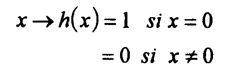
  
  ou :
  
  où deg(i) est le nombre de trajectoires potentielles avec lesquelles la trajectoire potentielle i est incompatible ;
• un terme a pour but d'exciter le neurone si celui-ci est désactivé et que la trajectoire potentielle associée n'est pas incompatible avec toutes les trajectoires potentielles correspondant aux neurones activés à la date où il est considéré. Autrement dit, si la sortie p _i du neurone i considéré vaut 0 à la date t(p _i (t)=0), alors cette correction est donnée par :
  
  où S est une fonction des sorties p _j (t) des autres neurones à la date t qui correspondent à des trajectoires potentielles incompatibles avec la trajectoire potentielle associée au neurone i . Par exemple :
  
     h : / R → {0,1} / R étant l'ensemble des réels
  
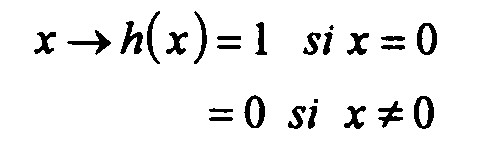
• ensuite, si le réseau a été mis à jour moins d'un certain nombre de fois préalablement fixé depuis la dernière convergence, alors on applique une excitation pour essayer d'augmenter, à la convergence suivante, la taille du sous-ensemble de trajectoires potentielles déterminé lors de la dernière convergence du réseau.

The correction to be applied to the potential u _i of a neuron i at a date t is determined . It is given by a linear combination of two terms:

• the purpose of a term is to inhibit neuron i if it is activated and the associated potential trajectory is incompatible with at least one of the potential trajectories corresponding to the neurons activated on the date it is considered. In other words, if the output p _i of neuron i at date t is equal to 1 ( p _i ( t ) = 1), then this correction is given by:
  
  where T is a function of the outputs p _i ( t ) of the neurons at date t which correspond to potential trajectories incompatible with the potential trajectory associated with neuron i . For example :
  
  with N the number of potential trajectories
  e _ij = 1 if the potential trajectories i and j are incompatible
  e _ij = 0 if the potential trajectories i and j are not incompatible (therefore are compatible)
  h : R → {0,1}
  
  or :
  
  where deg ( i ) is the number of potential trajectories with which the potential trajectory i is incompatible;
• the purpose of a term is to excite the neuron if it is deactivated and the associated potential trajectory is not incompatible with all the potential trajectories corresponding to the neurons activated on the date it is considered. In other words, if the output p _i of the neuron i considered is worth 0 at the date t ( p _i ( t ) = 0), then this correction is given by:
  
  where S is a function of the outputs p _j ( t ) of other neurons at date t which correspond to potential trajectories incompatible with the potential trajectory associated with neuron i . For example :
  
  h : / R → {0,1} / R being the set of reals
  
• then, if the network has been updated less than a certain number of times previously fixed since the last convergence, then an excitation is applied to try to increase, at the next convergence, the size of the subset of potential trajectories determined during the last convergence of the network.

Par exemple :

où :
   δ retourne 1 si le réseau de neurones a été mis à jour moins d'un certain nombre de fois fixé depuis la dernière convergence,
   l retoume 1 si N - deg(i) est supérieur à la plus grande taille des sous-ensembles de trajectoires potentielles trouvées jusqu'à la date t ;
   0 sinon.Otherwise, an interrupt process stops taking into account this excitation. This excitation can be written in the form:

For example :

or :
δ returns 1 if the neural network has been updated less than a certain number of times fixed since the last convergence,
l returns 1 if N - deg ( i ) is greater than the largest size of the subsets of potential trajectories found up to date t ;
0 otherwise.

The network therefore alternates pulsation phases (when this last excitation is taken into account) and relaxation phases (when the interruption process stops taking into account the excitation). During the relaxation phase, the network converges. Once the network has converged, an excitation is again applied (pulsation phase).

We thus alternate pulsation and relaxation phases a number of times, set by the user (depending on the time he has to find a solution, the quality of the solution he is looking for). At the end of each relaxation phase (at convergence), the neurons whose output is worth 1 encode a subset of potential trajectories two by two which are not incompatible, that is to say two by two compatible.

où A, B et C sont des réels positifs. Avantageusement, on prend A = B = C = 1.In general, the potential variation equations can be written, for all i belonging to {1, N }:

where A , B and C are positive reals. Advantageously, we take A = B = C = 1.

• on borne le potentiel entre des valeurs de l'ordre de grandeur des corrections à.appliquer au potentiel quand le neurone est mis à jour ;
• on borne les valeurs des potentiels entre -10^-∞ et 10^-∞ : ainsi toute correction strictement négative à appliquer sur le potentiel d'un neurone activé le désactive, et toute correction strictement positive à appliquer sur le potentiel d'un neurone désactivé l'active.

Advantageously, the potential of each neuron is bounded between two values set by the user to accelerate convergence. For example :

• the potential is bounded between values of the order of magnitude of the corrections to be applied to the potential when the neuron is updated;
• the values of the potentials are bounded between -10 ^-∞ and 10 ^-∞ : thus any strictly negative correction to be applied to the potential of an activated neuron deactivates it, and any strictly positive correction to be applied to the potential of a deactivated neuron l 'active.

Figure 5 illustrates a neuron i . FIG. 6 gives a first neural network associated with the device for implementing the method of the invention.

• une première mémoire 40 table des valeurs des sorties p _i des neurones recevant la sortie d'un circuit 39 de choix d'un entier allant de 1 à N ;
• une seconde mémoire 41 des relations entre objets ;
• une troisième mémoire 42 table des potentiels des neurones ;
• une quatrième mémoire 51 table des dernières variations de potentiels des neurones ;
• un premier circuit de calcul 43 permettant de calculer
  
• un second circuit de calcul 44 permettant de calculer
  
• un troisième circuit de calcul 45 permettant de calculer
  

ces trois circuits de calculs étant reliés aux sorties des deux premières mémoires ;

• un dispositif d'interruption 46 relié à la sortie du troisième circuit de calcul et aux sorties de la quatrième mémoire ;
• un premier additionneur 47 recevant les sorties des deux premiers circuits de calcul et du dispositif d'interruption ;
• un second additionneur 48 recevant les sorties de la troisième mémoire et du premier additionneur ;
• un circuit de fonction de seuillage à sortie binaire 49 recevant la sortie du second additionneur.

This first network includes:

• a first memory 40 table of the values of the outputs p _i of the neurons receiving the output of a circuit 39 for choosing an integer ranging from 1 to N ;
• a second memory 41 of the relationships between objects;
• a third memory 42 table of the potentials of the neurons;
• a fourth memory 51 table of the last variations of potentials of the neurons;
• a first calculation circuit 43 making it possible to calculate
  
• a second calculation circuit 44 making it possible to calculate
  
• a third calculation circuit 45 making it possible to calculate
  

these three calculation circuits being connected to the outputs of the first two memories;

• an interrupt device 46 connected to the output of the third calculation circuit and to the outputs of the fourth memory;
• a first adder 47 receiving the outputs of the first two calculation circuits and of the interruption device;
• a second adder 48 receiving the outputs of the third memory and of the first adder;
• a binary output thresholding function circuit 49 receiving the output of the second adder.

This network also includes a clock 50 connected to a random generator 51 connected to the circuit 39 for drawing an integer ranging from 1 to N.

The neural network evolves in asynchronous mode: one neuron is updated at a time.

We can demonstrate that a neural network thus defined converges (that is to say that there exists a date t for which ∀ i , ∀ t '> t , Δ u _i ( t ') = 0), in asynchronous mode at the end of each relaxation phase and that at convergence, all the strict constraints are satisfied.

b) The quality coefficients are reals

des sorties des neurones. On a les étapes suivantes :

• 1) Construction d'un réseau de neurones récursifs à partir des trajectoires potentielles et des relations entre les trajectoires potentielles en associant à chaque trajectoire potentielle la sortie binaire d'un neurone formel p _i ( _t ) :
     p _i (t) = 1 ⇒ la trajectoire potentielle appartient au sous-ensemble recherché,
     p _i (t) = 0 ⇒ la trajectoire potentielle n'appartient pas au sous-ensemble recherché.
• 2) Utilisation d'un procédé d'inhibition afin d'obtenir des sous-ensembles de trajectoires potentielles deux à deux non incompatibles. On passe d'un sous-ensemble à un autre en essayant d'augmenter la qualité de la solution.
• 3) Initialisation de la sortie et du potentiel associé à chaque neurone de telle sorte qu'ils vérifient, pour chaque neurone, les conditions suivantes :
  • sur les sorties des neurones : si on initialise un neurone i avec une sortie qui vaut 1 (neurone activé), alors les neurones j correspondant à des trajectoires potentielles incompatibles avec la trajectoire potentielle i (e _ij = 1) doivent être désactivés. $$\text{(}{\mathit{\text{p}}}_{\mathit{\text{i}}}\text{(}\mathit{\text{t}}\text{= 0)= 1) ⇒ (∀}\mathit{\text{j}}\text{ε{1,...,}\mathit{\text{N}}\text{} }{\mathit{\text{e}}}_{\mathit{\text{ij}}}\text{= 1 ⇒}{\mathit{\text{p}}}_{\mathit{\text{j}}}\text{(}\mathit{\text{t}}\text{= 0) = 0)}$$
    
  • sur les potentiels :
       p _i (t = 0) = 1 ⇔ u _i (t = 0) ≧ 0
       p _i (t = 0) = 0 ⇔ u _i (t = 0) ≦ 0
• 4) Exploitation dynamique récursive du réseau : on réalise une mise à jour de l'ensemble des neurones du réseau dans un certain ordre (par exemple aléatoire ou séquentiel) en considérant simultanément les neurones d'un bloc constitué d'un neurone i (centre) et les neurones voisins associés aux trajectoires potentielles incompatibles avec la trajectoire potentielle i (neurones j pour lesquels e _ij = 1).
  Pour mettre à jour ce bloc, on applique simultanément aux potentiels des neurones du bloc des corrections dépendantes des valeurs des sorties des autres neurones et des relations existant entre les trajectoires potentielles. L'expression mathématique de la correction à appliquer au potentiel d'un neurone diffère suivant qu'il est considéré comme centre d'un bloc ou comme voisin d'un centre d'un autre bloc.
  Les corrections sont définies de telle sorte que dès qu'un neurone i est activé, tous les neurones j vérifiant e _ij = 1 sont désactivés au même instant.
  L'exploitation dynamique génère des sous-ensembles de trajectoires potentielles deux à deux non incompatibles (donc deux à deux compatibles), chacun des sous-ensembles pouvant être associé à un maximum local de la fonction qualité.
  A chaque fois que le réseau a convergé, on obtient après décodage des sorties des neurones, un sous-ensemble de trajectoires potentielles deux à deux non incompatibles (donc deux à deux compatibles) maximisant (localement) la fonction qualité. On mémorise chacun de ces sous-ensembles. Globalement on obtient une liste de sous-ensembles solutions
• 5) Choix parmi les sous-ensembles listés du meilleur par comparaison des qualités

A second network of formal neurons is used and capable of determining a subset of potential trajectories two by two non-incompatible of maximum quality, where the quality is measured by any function

neuron outputs. We have the following stages:

• 1) Construction of a recursive neural network from potential trajectories and relationships between potential trajectories by associating with each potential trajectory the binary output of a formal neuron p _i ( _t ):
  p _i ( t ) = 1 ⇒ the potential trajectory belongs to the subset sought,
  p _i ( t ) = 0 ⇒ the potential trajectory does not belong to the subset sought.
• 2) Use of an inhibition process in order to obtain subsets of potential trajectories two by two that are not incompatible. We go from one subset to another while trying to increase the quality of the solution.
• 3) Initialization of the output and of the potential associated with each neuron so that they verify, for each neuron, the following conditions:
  • on the neuron outputs: if we initialize a neuron i with an output which is equal to 1 (activated neuron), then the neurons j corresponding to potential trajectories incompatible with the potential trajectory i ( e _ij = 1) must be deactivated. $$\text{((}{\mathit{\text{p}}}_{\mathit{\text{i}}}\text{((}\mathit{\text{t}}\text{= 0) = 1) ⇒ (∀}\mathit{\text{j}}\text{ε {1, ...,}\mathit{\text{NOT}}\text{}}{\mathit{\text{e}}}_{\mathit{\text{ij}}}\text{= 1 ⇒}{\mathit{\text{p}}}_{\mathit{\text{j}}}\text{((}\mathit{\text{t}}\text{= 0) = 0)}$$
    
  • on potentials :
    p _i ( t = 0) = 1 ⇔ u _i ( t = 0) ≧ 0
    p _i ( t = 0) = 0 ⇔ u _i ( t = 0) ≦ 0
• 4) Recursive dynamic exploitation of the network: we update all the neurons in the network in a certain order (for example random or sequential) by simultaneously considering the neurons of a block made up of a neuron i (center ) and the neighboring neurons associated with the potential trajectories incompatible with the potential trajectory i (neurons j for which e _ij = 1).
  To update this block, we apply simultaneously to the potentials of the neurons of the block corrections dependent on the values of the outputs of the other neurons and on the relationships existing between the potential trajectories. The mathematical expression of the correction to be applied to the potential of a neuron differs according to whether it is considered as the center of a block or as a neighbor of a center of another block.
  The corrections are defined such that as soon as a neuron i is activated, all the neurons j verifying e _ij = 1 are deactivated at the same time.
  Dynamic exploitation generates subsets of potential trajectories two by two which are not incompatible (therefore two by two compatible), each of the subsets being able to be associated with a local maximum of the quality function.
  Each time the network has converged, we obtain after decoding the neuron outputs, a subset of potential trajectories two by two non-incompatible (therefore two by two compatible) maximizing (locally) the quality function. Each of these subsets is memorized. Overall we obtain a list of solution subsets
• 5) Choice among the listed subsets of the best by comparison of the qualities

Recursive dynamic exploitation of this second neural network

We update the "block" of neurons ( i and the neurons j incompatible with i) corresponding synchronously (all the neurons of the block are updated simultaneously) by considering neuron i as "center" of the block and the neurons j as "neighbors" of the center.

The dynamic exploitation therefore consists in scanning all the blocks of neurons in a certain order (asynchronous dynamics) and in updating the neurons of each block in a synchronous manner: we speak of synchronous dynamics by block or block-synchronous.

Determination of the correction to be applied to the potential u _i of a neuron i on a date t

It differs according to whether the neuron whose potential is to be corrected is considered as the center of a block or as a neighbor of another center.

• si le neurone i est activé, on laisse le bloc inchangé ;
• si le neurone i est désactivé, on exécute les étapes qui suivent :
  • · on mémorise la valeur de la mesure de la qualité obtenue à la date
    
  • · on teste l'évolution suivante du réseau : on active le neurone i et on désactive les neurones j voisins si ceux-ci sont activés. On en déduit la variation de la mesure de la qualité correspondante

• A) La correction à appliquer au potentiel du neurone i est donnée par une combinaison linéaire de deux termes :
     - un terme qui a pour but d'exciter le neurone i , s'il est désactivé avec une certaine probabilité en fonction de la valeur de
  
  Par exemple l'excitation peut être donnée par :
  • · max
    
  • ·
    
  • · une procédure de Metropolis à une certaine température dans une méthode de recuit simulé,
  • · une procédure de Creutz à une certaine énergie dans une méthode de recuit microcanonique.
  
  Si le réseau a été mis à jour moins d'un certain nombre de fois depuis la dernière convergence, alors on applique une inhibition pour essayer d'augmenter, à la convergence suivante, la qualité du sous-ensemble de trajectoires potentielles déterminé lors de la dernière convergence du réseau. Autrement un procédé d'interruption stoppe la prise en compte de cette inhibition.
  Par exemple, cette inhibition peut consister à :
  • · inhiber un certain nombre de neurones, fixé par l'utilisateur, tirés aléatoirement,
  • · inhiber un nombre aléatoire de neurones tirés aléatoirement,
  • · inhiber des neurones parmi ceux qui correspondent à des trajectoires potentielles incompatibles avec beaucoup d'autres.
  
  Globalement, le réseau alterne des phases de pulsation (quand cette dernière inhibition est prise en compte) et des phases de relaxation (quand le procédé d'interruption stoppe la prise en compte de l'inhibition). Au cours de la phase de relaxation, le réseau converge. Une fois que le réseau a convergé, on applique à nouveau une inhibition (phase de pulsation). On alterne ainsi des phases de pulsation et de relaxation un certain nombre de fois, fixé par l'utilisateur (en fonction du temps qu'il a pour trouver une solution, de la qualité de la solution qu'il recherche). A l'issue de chaque phase de relaxation, c'est-à-dire à chaque convergence, les neurones dont la sortie vaut 1 codent un sous-ensemble de trajectoires potentielles deux à deux non en relation.
• B) La correction à appliquer au potentiel du neurone j voisin de i à la date t est donnée par un terme qui a pour but d'inhiber le neurone j d'une quantité égale à l'excitation reçue par le neurone i à la même date. Par exemple, l'inhibition peut être donnée par :
  • ·
    
    si l'excitation sur i à t vaut
    
  • ·
    
    si l'excitation sur i à t vaut

When we consider a block of neurons with center i and neighbors V = { j } (for all j in V , e _ij = 1) at date t , we look at whether neuron i is activated or not:

• if neuron i is activated, the block is left unchanged;
• if neuron i is deactivated, the following steps are carried out:
  • · The value of the quality measurement obtained on the date is memorized
    
  • · We test the following evolution of the network: we activate neuron i and deactivate neighboring neurons j if these are activated. We deduce the variation of the corresponding quality measure

• A) The correction to be applied to the potential of neuron i is given by a linear combination of two terms:
  - a term which aims to excite neuron i , if it is deactivated with a certain probability as a function of the value of
  
  For example, excitement can be given by:
  • · Max
    
  • ·
    
  • · A Metropolis procedure at a certain temperature in a simulated annealing method,
  • · A Creutz procedure at a certain energy in a microcanonical annealing method.
  
  If the network has been updated less than a certain number of times since the last convergence, then an inhibition is applied to try to increase, at the next convergence, the quality of the subset of potential trajectories determined during the last convergence of the network. Otherwise an interrupt process stops taking this inhibition into account.
  For example, this inhibition can consist of:
  • · Inhibit a number of neurons, set by the user, randomly drawn,
  • · Inhibit a random number of neurons randomly drawn,
  • · Inhibit neurons among those that correspond to potential trajectories incompatible with many others.
  
  Overall, the network alternates pulsation phases (when this last inhibition is taken into account) and relaxation phases (when the interruption process stops taking into account the inhibition). During the relaxation phase, the network converges. Once the network has converged, an inhibition (pulse phase) is again applied. We thus alternate pulsation and relaxation phases a number of times, set by the user (depending on the time he has to find a solution, the quality of the solution he is looking for). At the end of each relaxation phase, that is to say at each convergence, the neurons whose output is equal to 1 code a subset of potential trajectories two by two not in relation.
• B) The correction to be applied to the potential of neuron j near i on date t is given by a term which aims to inhibit neuron j by an amount equal to the excitation received by neuron i at the same dated. For example, inhibition can be given by:
  • ·
    
    if the excitation on i at t is worth
    
  • ·
    
    if the excitation on i at t is worth

• on borne le potentiel entre des valeurs de l'ordre de grandeur des corrections à appliquer au potentiel quand le neurone est mis à jour ;
• on borne les valeurs des potentiels entre -10^-∞ et 10^-∞ : ainsi toute correction strictement négative à appliquer sur le potentiel d'un neurone activé le désactive et toute correction strictement positive à appliquer sur le potentiel d'un neurone désactivé l'active.

Advantageously, the potential of each neuron is bounded between two values set by the user to accelerate convergence. For example :

• the potential is bounded between values of the order of magnitude of the corrections to be applied to the potential when the neuron is updated;
• we limit the values of the potentials between -10 ^-∞ and 10 ^-∞ : thus any strictly negative correction to be applied to the potential of an activated neuron deactivates it and any strictly positive correction to be applied to the potential of a deactivated neuron active.

• une première mémoire 55 table des valeurs des sorties p _i des neurones ;
• une seconde mémoire 56 table des voisins de chaque neurone ;
• une troisième mémoire 57 des relations entre les objets ;
• une quatrième mémoire 58 des potentiels des neurones ;
• une cinquième mémoire 67 ;
• un premier circuit de calcul 59 permettant de calculer la variation de potentiel à appliquer au neurone i ;
• un second circuit de calcul 60 permettant de calculer la variation de potentiel à appliquer aux neurones voisins du neurone i ;
• un premier additionneur 61 recevant les sorties du premier circuit de calcul et de la quatrième mémoire ;
• au moins un second 62 additionneur recevant les sorties du second circuit de calcul et de la quatrième mémoire ;
• au moins deux circuits 64 et 65 fonctions de seuillage binaire F reliés respectivement aux sorties de ces deux additionneurs.

Figure 7 shows a device associated with the second neural network. This second network includes:

• a first memory 55 table of the values of the outputs p _i of the neurons;
• a second memory 56 table of neighbors of each neuron;
• a third memory 57 of the relationships between the objects;
• a fourth memory 58 of the potentials of the neurons;
• a fifth memory 67;
• a first calculation circuit 59 making it possible to calculate the variation in potential to be applied to neuron i ;
• a second calculation circuit 60 making it possible to calculate the variation in potential to be applied to the neurons neighboring neuron i ;
• a first adder 61 receiving the outputs of the first calculation circuit and the fourth memory;
• at least a second adder 62 receiving the outputs of the second calculation circuit and of the fourth memory;
• at least two circuits 64 and 65 binary thresholding functions F respectively connected to the outputs of these two adders.

In the case of a digital device these different elements are connected (directly or indirectly) to a clock.

The algorithms described above have been applied to many images of fluid mechanics. A trajectory in these images is made up of three consecutive and aligned points. The ambiguity on the direction is removed by the use of a particular coding of the pulses: the duration between the first two pulses is equal to twice the duration between the two second pulses.

We will now study an example of the results of the various treatments carried out in the process of the invention, by successively considering the two cases analyzed above.

a) Case where the quality coefficients ( F ₂ ( i , j )) are real

Figures 8, 9 and 10 show the results of the different treatments performed. Thus, Figure 8 shows the original image. The size of this image is 1500 * 1000 pixels. FIG. 9 presents the potential trajectories which were generated at the end of step 12. From the original image 8, 6664 points were extracted and 1303 potential trajectories (triplets of points) were generated. The processing (steps 11 and 12) required 1030ms, on a standard workstation of the SUN SPARC 10 type. The time required to perform steps 13 and 14 (determination of the constraints and calculation of the qualities between pairs of signals) required 2390ms . Finally the last stage of the processing required 2880ms, a total for the total image processing of 6290ms. FIG. 10 represents the final result provided by the algorithm using real quality coefficients. In this image 775 particle trajectories have been recognized.

b) Case where the quality coefficients ( F ₂ ( i , j)) are binary

The initial image and the image of the potential triplets generated are the same as above, namely FIGS. 8 and 9 respectively. The result of the neuromimetic network processing provides image 11. 510 trajectories were extracted in 1 min 4680 ms (time required for steps 13, 14 and 15).

LEXICON Object

An object has a physical reality. It is for example a particle, an air bubble, a glitter, a star, ... The process aims to automatically determine the trajectories of various objects over time.

Fragment

A fragment is a record of the position in space of an object on a certain date. The method processes a set of fragments.

Fragment class

The process will segment all of the fragments into classes, each of which is characteristic of a single object recorded at various times. A particular class corresponds to the fragments that the process has not associated with objects. All fragments of this class are considered noise, in the sense of signal processing. The classes must be two to two disjoint. The number of fragments in a characteristic class of an object is an input to the process: it is the number of times at which recordings are made.

Path

A trajectory is a class of fragments associated with an object.

Neuron

• on calcule une correction Δu _i(t) à appliquer au potentiel u _i (t + 1)= u _i (t)+ Δu _i (t) ;
• on met à jour la sortie :

   si u _i (t + 1) > 0 alors p _i (t + 1) = 1
   si u _i (t + 1) < 0 alors p _i (t + 1) = 0

neurone activé

p _i = 1

neurone désactivé

p _i = 0

A neuron i is defined by a potential u _i and by a binary output p _i . When, during dynamic network operation, the neuron is considered at date t , then:

• we calculate a correction Δ u _i ( t ) to apply to the potential u _i ( t + 1) = u _i ( t ) + Δ u _i ( t );
• we update the output:

if u _i ( t + 1)> 0 then p _i ( t + 1) = 1
if u _i ( t + 1) <0 then p _i ( t + 1) = 0

activated neuron

p _i = 1

neuron disabled

p _i = 0

Relationship

Expression of the compatibility of two potential trajectories in a velocimetry application, of two resource / demand pairs in a resource allocation application, and more generally an edge between the nodes of a graph, ...

We have a set of potential trajectories from which we seek to extract a subset verifying a certain property based on relations between the potential trajectories. Considered two by two, there exists or not a relation (resulting from an application) between the potential trajectories.

If a potential trajectory i is in relation to a potential trajectory j , then e _ij = 1. Otherwise e _ij = 0. ( e _ij ) is the matrix of the relations between the potential trajectories.

Claims (13)

Method for obtaining trajectories of moving objects, by optimizing at least one criterion from the physics of the phenomenon observed, characterized in that it comprises the following steps: - A step (10) of recording signals composed of fragments characteristic of the positions of objects at different times, of parts which have the same nature as the fragments but which are noise and parts attributable to noise without possible confusion; a step (11) of extracting parts of signals having the same nature as the fragments and determining the characteristics associated therewith, from a priori knowledge of their nature and of the trajectories sought; - a step (12) of distributing all the parts of signals previously extracted into classes, each class representing a potential trajectory and comprising a predetermined number of fragments; a step (13, 14) of selecting a subset of classes which satisfies the constraints linked to the type of network observed, comprising: · The generation of a set of n-tuples made up of a subset of n classes, · The measurement of the compatibility of the classes assembled in n-tuples by a first analytical function ( F 1), determined from the constraints related to the type of phenomenon observed and to the acquisition device, · The measurement of the quality of the tuples by a second analytical function ( F 2), determined from the constraints linked to the observed phenomenon and to the acquisition device; a step (15) of selection from among the classes representing the potential trajectories of those satisfying the constraints, by a method of optimization under constraints of the previous criterion (s), using the previous compatibility measures and of quality, so as to obtain the "real" trajectories of the objects. Method according to claim 1, characterized in that in the first step the position of the objects is recorded at several distinct and consecutive times, separated by fixed time intervals. A method according to claim 1, characterized in that during the recording step, when it is impossible to work in real time, the processing for conditioning the signals obtained comprises a substep of memorizing the signals. Method according to claim 3, characterized in that the signals are preprocessed before their storage. Method according to claim 1, characterized in that the tuples are pairs. Method according to claim 1, characterized in that the last step of selecting subsets of mutually compatible forms is carried out using a neural network. Method according to any one of the preceding claims, characterized in that it can be used for the extraction of given forms in a noisy environment. Method according to any one of the preceding claims, characterized in that the objects are particles. Device for implementing the method according to any one of the preceding claims, characterized in that it comprises: - a recording device (20); - a feature extraction module (21); - a module for generating potential trajectories (22); - a problem shaping module (23); - a module for solving the optimization problem (24). Device according to claim 9, characterized in that the recording device (20) comprises: - a signal sampling stage (31); - an acquisition stage (30); - a recording stage (31). Device according to claim 9, characterized in that the optimization problem solving module (24) comprises a neural network. Device according to claim 11, characterized in that this neuron network comprises: - a first memory (40) table of the outputs p _i of the neurons receiving the output of a circuit for choosing an integer ranging from 1 to N ; - a second memory (41) of the relationships between objects; - a third memory (42) table of the potentials of the neurons; - A fourth memory (51) table of the last variations of the potentials of the neurons; - a first calculation circuit (43) for calculating

- a second calculation circuit (44) for calculating

- a third calculation circuit (45) for calculating

these three calculation circuits being connected to the outputs of the first two memories; - an interrupt device (46) connected to the output of the third calculation circuit and to the outputs of the fourth memory; - a first adder (47) receiving the outputs of the first two calculation circuits and of the interruption device; - a second adder (48) receiving the outputs of the third memory and of the first adder; - a binary output thresholding function circuit (49) receiving the output of the second adder. Device according to claim 11, characterized in that this neural network comprises: - a circuit for choosing an integer between 1 and N - a first memory (55) table of the values of the outputs p _i of the neurons; - a second memory (56) list of the neighbors of each neuron; - a third memory (57) relation between the objects; - A fourth memory (58) of the potentials of the neurons; - a fifth memory (67) containing the current value of the measurement E to be optimized; - a first calculation circuit (59) for calculating the variation in potential to be applied to the neuron; - a second calculation circuit (60) making it possible to calculate the variation in potential to be applied to the neurons neighboring neuron i ; - a first adder (61) receiving the outputs of the first calculation circuit and of the fourth memory; - at least one second adder (62, 63) receiving the outputs of the second calculation circuit and of the fourth memory; - at least two binary thresholding function circuits F (64 and 65) connected respectively to the outputs of these two adders.

Images