EP2943935B1 - Estimation of the movement of an image - Google Patents
Estimation of the movement of an image Download PDFInfo
- Publication number
- EP2943935B1 EP2943935B1 EP14703136.3A EP14703136A EP2943935B1 EP 2943935 B1 EP2943935 B1 EP 2943935B1 EP 14703136 A EP14703136 A EP 14703136A EP 2943935 B1 EP2943935 B1 EP 2943935B1
- Authority
- EP
- European Patent Office
- Prior art keywords
- term
- image
- points
- data
- estimation
- Prior art date
- Legal status (The legal status is an assumption and is not a legal conclusion. Google has not performed a legal analysis and makes no representation as to the accuracy of the status listed.)
- Active
Links
- 230000033001 locomotion Effects 0.000 title claims description 70
- 238000000034 method Methods 0.000 claims description 66
- 239000013598 vector Substances 0.000 claims description 66
- 230000033228 biological regulation Effects 0.000 claims description 21
- 230000001788 irregular Effects 0.000 claims description 9
- 238000004590 computer program Methods 0.000 claims description 4
- 238000006073 displacement reaction Methods 0.000 description 24
- 238000004364 calculation method Methods 0.000 description 17
- 239000011159 matrix material Substances 0.000 description 17
- 238000001914 filtration Methods 0.000 description 5
- 230000003750 conditioning effect Effects 0.000 description 3
- 238000009499 grossing Methods 0.000 description 3
- 241000897276 Termes Species 0.000 description 2
- 230000001364 causal effect Effects 0.000 description 2
- 238000006243 chemical reaction Methods 0.000 description 2
- 230000003247 decreasing effect Effects 0.000 description 2
- 230000003287 optical effect Effects 0.000 description 2
- 230000002123 temporal effect Effects 0.000 description 2
- LZDYZEGISBDSDP-UHFFFAOYSA-N 2-(1-ethylaziridin-1-ium-1-yl)ethanol Chemical compound OCC[N+]1(CC)CC1 LZDYZEGISBDSDP-UHFFFAOYSA-N 0.000 description 1
- 230000001133 acceleration Effects 0.000 description 1
- 238000007796 conventional method Methods 0.000 description 1
- 238000009795 derivation Methods 0.000 description 1
- 238000009792 diffusion process Methods 0.000 description 1
- 230000010354 integration Effects 0.000 description 1
- 230000000717 retained effect Effects 0.000 description 1
- 238000007493 shaping process Methods 0.000 description 1
- 230000006641 stabilisation Effects 0.000 description 1
- 238000011105 stabilization Methods 0.000 description 1
- 230000001960 triggered effect Effects 0.000 description 1
Images


Classifications
-
- H—ELECTRICITY
- H04—ELECTRIC COMMUNICATION TECHNIQUE
- H04N—PICTORIAL COMMUNICATION, e.g. TELEVISION
- H04N19/00—Methods or arrangements for coding, decoding, compressing or decompressing digital video signals
- H04N19/50—Methods or arrangements for coding, decoding, compressing or decompressing digital video signals using predictive coding
- H04N19/503—Methods or arrangements for coding, decoding, compressing or decompressing digital video signals using predictive coding involving temporal prediction
- H04N19/51—Motion estimation or motion compensation
- H04N19/513—Processing of motion vectors
-
- G—PHYSICS
- G06—COMPUTING; CALCULATING OR COUNTING
- G06T—IMAGE DATA PROCESSING OR GENERATION, IN GENERAL
- G06T7/00—Image analysis
- G06T7/20—Analysis of motion
- G06T7/269—Analysis of motion using gradient-based methods
-
- G—PHYSICS
- G06—COMPUTING; CALCULATING OR COUNTING
- G06T—IMAGE DATA PROCESSING OR GENERATION, IN GENERAL
- G06T7/00—Image analysis
- G06T7/20—Analysis of motion
- G06T7/254—Analysis of motion involving subtraction of images
-
- G—PHYSICS
- G06—COMPUTING; CALCULATING OR COUNTING
- G06T—IMAGE DATA PROCESSING OR GENERATION, IN GENERAL
- G06T7/00—Image analysis
- G06T7/20—Analysis of motion
- G06T7/277—Analysis of motion involving stochastic approaches, e.g. using Kalman filters
-
- H—ELECTRICITY
- H04—ELECTRIC COMMUNICATION TECHNIQUE
- H04N—PICTORIAL COMMUNICATION, e.g. TELEVISION
- H04N19/00—Methods or arrangements for coding, decoding, compressing or decompressing digital video signals
- H04N19/42—Methods or arrangements for coding, decoding, compressing or decompressing digital video signals characterised by implementation details or hardware specially adapted for video compression or decompression, e.g. dedicated software implementation
- H04N19/43—Hardware specially adapted for motion estimation or compensation
-
- H—ELECTRICITY
- H04—ELECTRIC COMMUNICATION TECHNIQUE
- H04N—PICTORIAL COMMUNICATION, e.g. TELEVISION
- H04N5/00—Details of television systems
- H04N5/14—Picture signal circuitry for video frequency region
- H04N5/144—Movement detection
- H04N5/145—Movement estimation
-
- G—PHYSICS
- G06—COMPUTING; CALCULATING OR COUNTING
- G06T—IMAGE DATA PROCESSING OR GENERATION, IN GENERAL
- G06T2207/00—Indexing scheme for image analysis or image enhancement
- G06T2207/10—Image acquisition modality
- G06T2207/10016—Video; Image sequence
Definitions
- the invention relates to the field of image processing, and more particularly to the field of motion estimation within a captured image sequence.
- a sensor When a sensor captures a sequence of successive images, for example in the case of a video, it is known to perform an overall motion estimation between images. This motion estimation is intended to determine the overall motion affecting the sequence of images between successive pairs of images of the sequence and may correspond to the determination of the movement of the line of sight of the sensor used.
- Such global motion estimation makes it possible, in particular, to implement image stabilization, image denoising, or even super-resolution algorithms.
- this type of processing can be substantially disturbed when the captured scene includes objects that are movable in the scene during the sequence of images in question.
- Image processing systems are then based on the implementation of a motion estimation no longer global but dense, also called "local motion estimation”.
- a dense motion estimation consists in estimating the motion at each point P ( x , y ), or pixel, of the images of the captured sequence. More precisely, a displacement field d ( x , y ) is defined from two images and corresponds to the vectors to be applied respectively to each point of the first image to obtain the corresponding point of the second image.
- the field of speed v ( x , y ) can be interesting.
- This velocity field is also called optical flow and is formed by the set of velocity vectors at a given moment of each point of the image. This velocity field is a function of the derivative of the displacement field with respect to a fixed reference.
- I x there t I x + dx , there + dy , t + dt
- I x there t I x + dx , there + dy , t + dt
- I x , y , t is a luminous intensity value (hereinafter referred to as "intensity") of a point P (x , y) of the scene at a time t of capture of an image called the preceding image I k -1 .
- next image I k is captured at a time t + dt and dt then corresponds to the time interval between the two images I k -1 , I k .
- (dx, dy) d ( x , y ) denotes the displacement vector of the point P (x , y) between the instants t and t + dt .
- the Horn-Schunck method imposes a hypothesis of regularity of the velocity field which limits its efficiency in the presence of discontinuities of the velocity field. Its resolution is also done by gradient descent and is therefore slow.
- Lucas-Kanade method assumes the local constancy of the velocity field. It is robust to noise but has the disadvantage of being sparse, that is to say that it does not make it possible to estimate the velocity fields at the points in the vicinity of which the intensity vector spatial gradient is locally uniform.
- substantially uniform is meant that the intensity vector spatial gradients at the different points of the neighborhood considered are either substantially parallel to each other or substantially zero.
- substantially zero is meant that the norm of a vector spatial gradient of intensity considered is lower than the noise of the image.
- any of the scalar components for example ⁇ I ⁇ x or ⁇ I ⁇ there ) of the vector (intensity) spatial gradient, which is a vector.
- vector intensity intensity gradient and “vector intensity spatial gradient” will also be used interchangeably.
- any of the scalar components for example ⁇ I ⁇ x ⁇ I ⁇ there or ⁇ I ⁇ t ) of the vector-intensity (intensity) spatio-temporal gradient.
- the invention aims to improve the situation.
- a first aspect of the invention proposes a motion estimation method in a series of images captured by an image sensor, said series of images comprising at least one preceding image I k -1 and a next image I k, images with points which are associated intensity data.
- the method comprises an estimated motion vector estimation step V , performed at a plurality of points of an image chosen from the list consisting of the previous image I k -1 and the following image I k .
- the estimation step includes, for each of the points P of said plurality of points of an image, an operation of minimizing a functional J of motion vectors V.
- the functional J comprises a sum of at least one term term term data and a term term regulation term.
- the term of the data is a function of spatio-temporal gradients of intensity data associated with a plurality of points of a neighborhood ⁇ P of a point P.
- the term of the data is a function of the spatial gradients. vector temporals of associated intensity data (i.e., each of their scalar components).
- the control term has a finite value at least in each of the points P of said plurality of points of an image at which the minimization of the data term provides an irregular solution.
- a solution is irregular if the minimization of the term of attachment to the data does not make it possible to estimate a single solution.
- the term data includes a product of a term called weighting term and a term term term of attachment to the data, the weighting term being a function of a degree of regularity of estimated motion vectors V , the term of attachment to the datum being a function of spatio-temporal gradients of intensity data associated with a plurality of points of a neighborhood ⁇ P of a point P.
- the term of attachment to the data is a function of the vector spatio-temporal gradients of associated intensity data (that is, of each of their scalar components).
- Previous image and “next image” of a series of captured images, two images that follow each other chronologically in the series of images considered. These two images that follow can be consecutive (that is to say, not be separated by any intermediate captured image) or else spaced apart by one or more intermediate captured images. No limitation is attached to the spacing between the previous image and the next image considered here.
- estimate of estimated motion vectors is intended to mean an estimation method making it possible to provide estimated motion vectors for each part of the image, with more or less precision. An image movement can thus be estimated at each point of the image for example.
- This type of motion estimation makes it possible to represent in particular the movement of moving objects that could pass through the images of the series of captured images.
- those skilled in the art know in particular the methods of Lucas-Kanade and Horn-Schunck.
- a first method consists in solving the equation of the least-squares motion on a local window.
- a second method extracted from the article by Berthold KP Horn and Brian G. Schunck, "Determining optical flow” (ARTIFICAL INTELLIGENCE, 1981), consists of a minimization of a functional including a term of attachment to the data comprising the square of the apparent motion equation, and a regularization term including the square of the local variation of the field.
- data refers to the set of intensity data of the points of an image.
- the "data term” and the “data term” are terms that are a function of the spatio-temporal gradients of intensity at points in a neighborhood ⁇ 0 of a point P 0 ( x 0 , y 0 ).
- the extent of this neighborhood ⁇ 0 for example the maximum distance of the points comprised in this neighborhood with respect to the point P 0 , as well as a weighting of each of these points in a calculation of term of attachment to the datum may be variables according to the conditions of use of the process.
- regulation term is meant a term having a finite value at least in each of the points P 0 of the image at which the minimization of the term of the data provides an irregular solution.
- the minimization of the data term provides an uneven solution in homogeneous regions and regions of low angular diversity.
- the homogeneous regions are regions of substantially constant intensity and therefore in which the modules of the vector spatial gradients of the intensities are substantially zero (below a determined threshold, which may correspond to a noise level).
- the associated vector spatial gradients of intensity at different points in the region are substantially parallel.
- the angular diversity is measured for example by the variance of the set of angles defined respectively by a pair of gradients, for all possible pairs of gradients chosen in all of the gradients considered.
- a region of low angular diversity is a region in which the angular diversity of the vector intensity spatial gradients associated with the various points of the region is substantially zero (below a determined threshold, which may correspond to a noise level).
- a finite value of a term is a real or imaginary value, unique and not infinite. Such a finite value may be defined prior to an estimation step or computable by means of a regular function defined on an interval having a point P 0 .
- a regulation term thus makes it possible to smooth a motion vector field by providing a solution to the problem of minimizing a functional at the levels of the points of an image where the minimization of a term of attachment to the datum makes it impossible to estimate a single solution.
- weighting term is meant a term for weighting the relative importance of terms of attachment to the data and of regulation terms, the weighting being performed as a function of a spatial gradient of the intensity data in a neighborhood of a point P 0 .
- the weighting is performed according to a vector spatial gradient of the intensity data in a neighborhood of a point P 0 .
- estimated degree of motion vector regularity is meant a function of the variance of the estimated motion vector field.
- the invention also relates to a system for processing a series of images captured by an image sensor, said series of images comprising at least one preceding image I k -1 and a following image I k , the images each having points with associated intensity data
- the system comprising an estimation circuit adapted to estimate estimated motion vectors V at a plurality of points of an image selected from the list constituted by the preceding image I k -1 and the following image I k, said estimate comprising, for each of the points P of said plurality of points of an image, a minimization operation of a functional element J of motion vectors V , the functional J comprising a sum of at least one term of the data and a regulation term, the term of the data being a function of spatio-temporal gradients of intensity data associated with a plurality of points of a neighborhood ⁇ P of a point P, the regulation term having at least one finite value at each of the points P of said plurality of points of an image at which the minimization of the term of the data provides an irregular solution, the
- the subject of the invention is also a computer program comprising instructions able to implement a method as described above, when executing this program by a circuit of a series processing system. Images captured by an image sensor.
- the invention finally relates to a non-transitory recording medium on which is stored a computer program as described above.
- the speed field can be assumed locally constant on a neighborhood ⁇ 0 of each point P 0 ( x 0 , y 0 ) .
- Solving the system of least squares equation (5) requires inverting a 2x2 size matrix. This inversion is only possible at points having an angular diversity of spatial gradients of sufficiently high intensity, as specified above, for example points in the vicinity of which there are at least two points including spatial gradients vector of light intensity have substantially distinct directions.
- an image 1 may for example be formed of a clear homogeneous region 2 as well as of a dark homogeneous region 3 of generally rectangular shape.
- a first neighborhood 4 having for example the general shape of a disc centered on one of the vertices of the dark homogeneous region 3, will therefore comprise vector spatial gradients of intensity in two different directions 4a and 4b, for example following the horizontal direction and the vertical direction. A displacement of the dark homogeneous region 3 can then be completely determined in this vicinity.
- a second neighborhood 5, similar in shape to the first neighborhood 4 and located for example at one of the vertical edges of the dark homogeneous 3, comprises a vector spatial gradient of the intensity only in a direction 5a, for example the horizontal direction.
- the displacement of the homogeneous dark region 3 can not be completely determined.
- a third neighborhood 6 also of similar shape to the first neighborhood 4, is for example located entirely in the light homogeneous region 2. In this vicinity 6, the vector spatial gradient of the intensity is substantially zero and the estimate of the field of displacement is therefore impossible.
- J v x v there x 0 there 0 ⁇ v x v there ⁇ x there ⁇ ⁇ 0 W x - x 0 , there - there 0 ⁇ I ⁇ x x there v x x 0 there 0 + ⁇ I ⁇ there x there v there x 0 there 0 + ⁇ I ⁇ t 2 + ⁇ 2 v x - v ⁇ x 2 + v there - v ⁇ there 2
- This functional has three terms: a term of attachment to the data, a term of weighting according to the degree of regularity of the estimated field and a term of regulation, which will now be detailed.
- the functional consists of the product of the weighting term and the term of attachment to the datum, to which is added the term of regulation.
- ⁇ x there ⁇ ⁇ 0 W x - x 0 , there - there 0 ⁇ I ⁇ x x there v x x 0 there 0 + ⁇ I ⁇ there x there v there x 0 there 0 + ⁇ I ⁇ t 2 of the above equation (6) is a term of attachment to the datum which takes into account the local constancy of the velocity field in a neighborhood ⁇ 0 of the point P 0 ( x 0 , y 0 ) , in a manner similar to the functional H of equation (5) above.
- the minimization of this term makes it possible to estimate a velocity field as a function of the spatio-temporal gradients of the luminous intensity.
- ⁇ ( v x , v y ) of the preceding equation (6) is a weighting term as a function of the degree of regularity of the estimated field of the term of attachment to the datum. This term makes it possible to reduce the importance of the term of attachment to the data in the homogeneous and one-dimensional regions.
- a function of the form ⁇ ((var ( v x , v y )) can be used for the term ⁇ ( v x , v y ), the function being a decreasing function with a value between 0 and 1 and var (v x , v y ) being the variance of the velocity field at the point P 0 ( x 0 , y 0 ) or in a neighborhood of the point P 0 ( x 0 , y 0 ).
- velocity field is irregular, the variance var ( v x , v y ) is high and the weighting term is close to 0. If, instead, the estimate is regular, the variance is small and the weighting term will be close 1.
- a weighting term ⁇ ( v x , v y) may be used where v x and v y are averages of the velocity field on a neighborhood of the point P 0 ( x 0 , y 0 ).
- ⁇ x ⁇ 1 / (1+ ( x / 0.02) 2 ) which is a decreasing function with values between 0 and 1.
- weighting term may be used as soon as they provide a low-value term in areas where the estimate provided by the term attachment to the data is unreliable.
- the weighting term can in particular include a weighting term of the homogeneous regions, for example of the form ⁇ ( ⁇ + / g ) where ⁇ is a positive increasing function on [0, + ⁇ [, ⁇ + is a function of the spatio gradients -temporels intensity (e.g., greater eigenvalue of the matrix P gradients of which is detailed below) and g is a weighting threshold value.
- ⁇ is a positive increasing function on [0, + ⁇ [, ⁇ + is a function of the spatio gradients -temporels intensity (e.g., greater eigenvalue of the matrix P gradients of which is detailed below) and g is a weighting threshold value.
- ⁇ is a positive increasing function on [0, + ⁇ [, ⁇ + is a function of the spatio gradients -temporels intensity (e.g., greater eigenvalue of the matrix P gradients of which is detailed below)
- g is a weighting
- ⁇ 2 ( v x - v x) + ( v y - v y ) 2 ) of the above equation (6) is a control term.
- Average values v x and v there correspond to the average values of the velocity field components on a neighborhood of the point P 0 ( x 0 , y 0 ) respectively taken along the axis Ox and the axis Oy .
- the regulation term makes it possible to replace the estimation of the velocity field provided by the term of attachment to the datum by the average value of said field over a neighborhood of the point P 0 ( x 0 , y 0 ).
- this replacement is performed only at the points P 0 ( x 0 , y 0 ) for which said estimate is irregular due either to an absence of gradient (that is, substantially zero gradients) or substantially parallel vector spatial gradients.
- the least squares functional J at the point P 0 ( x 0 , y 0 ) of equation (6) is minimized by a matrix method.
- This method consists in putting the functional J in matrix form before deriving it and canceling this derivative to obtain a solution of the speed field at the iteration n : V n .
- the sums ⁇ of the matrix P can be understood as being the sums of the points P i (x i, y i) of the neighborhood ⁇ 0 of the point P 0 (x 0, y 0), and the terms W and spatial gradients -temporal intensity are taken at said points P i ( x i , y i ) .
- W correspond to the window function W 0 ( x , y ) defined above, which makes it possible to weight on all the points of the neighborhood ⁇ 0 of the point P 0 ( x 0 , y 0 ).
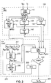
- a motion estimation method comprises two steps, a preliminary calculation step 100 followed by an iterative calculation step of the speed field 200.
- This series of images comprises at least one previous image I k-1 and a subsequent image I k .
- the first step 100 is to initialize the basic terms.
- It comprises a first operation 110 for calculating the spatio-temporal derivatives of the intensity from the preceding images I k-1 and following I k .
- the points of the image may be chosen as corresponding to the points of the previous image, the next image or in a repository different from the two images.
- the matrix Q - ⁇ W 2 I x I t - ⁇ W 2 I there I t is evaluated.
- a fourth operation 140 makes it possible to calculate the regulation matrix R for example in the manner detailed above in equation (10).
- a fifth operation 150 may comprise the determination of a weighting level of the homogeneous regions on the basis of the eigenvalues of the matrix P.
- the homogeneous regions correspond in fact to the regions in which the eigenvalues of the matrix P are small values, and a weighting threshold value for the eigenvalues of the matrix P can therefore be fixed to allow weighting of the homogeneous regions.
- motion vectors are estimated at a plurality of points of an image chosen from the preceding image I k-1 and the following image I k .
- a set 201 of values of the velocity field v x , v y at each point P 0 ( x 0 , y 0 ) of the image is firstly initialized. These values correspond to the speed field V 0 at the iteration 0.
- a second operation 220 will consist of a calculation of the weighting term ⁇ ( V n ), which calculation may use the average values of the field determined during the first operation 210 detailed above.
- a third operation 230 consists in solving the equation (10) for obtaining the new velocity field V n +1 of the step n + 1 from the matrices determined during the preliminary step 100 as well as results of the first 210 and second 220 operations of the calculation step 200.
- a fourth step 240 the opportunity to stop the iterative calculation is evaluated against a predefined criterion.
- This criterion can constitute to compare the number n of the current iteration with a maximum iteration number n max , that is to say to evaluate the condition n ⁇ n max .
- the iterative calculation step 200 ends and returns the last estimated velocity field V n max .
- the counter of the number of iteration n is incremented during a fifth step 250 and the estimated speed field V n serves as an initial value for a new calculation of step 200. It is therefore used as initial value for a new operation 210 for determining the averages of the velocity field.
- the following operations 220, 230, 240 are then repeated.
- Another criterion for the fourth step 240 may comprise the comparison of a difference between the speed field obtained at the end of the third step 230 V n +1 and the speed field obtained at the previous iteration V n .
- a criterion may consist in evaluating the following condition ⁇ V n +1 - V n ⁇ ⁇ ⁇ where ⁇ is a predefined value.
- the first-order development (2) of the apparent motion constraint equation (1) detailed above is valid only for small displacements, for example of the order of the pixel. To measure large displacements, it is therefore advantageous to perform a multi-scale calculation.
- the multi-scale motion estimation method 400 is applied to a series of images I i , for i integer between 1 and N , this series of images comprising at least one preceding image I k-1 and a following image I k .
- a first step 410 the previous images I k-1 and following I k are scaled to give images scaled I k-1 s , I k s .
- This step may include applying an anti-aliasing filter and then decimating the image.
- An anti-aliasing filter is sometimes also referred to as an anti-aliasing filter or anti-aliasing filter and consists in removing, before decimation, frequencies greater than half the decimation frequency.
- the images may also be pre-filtered to filter the high frequencies, for example by pyramidal filters.
- one of the images for example the following image set to the scale I n s is recaled according to the displacement field D c determined at the previous iteration, to give a next image scaled up I n s, d .
- the displacement field D c and the scale Scl are initialized to zero.
- a third step 430 comprises executing a motion estimation method according to an embodiment of the present invention comprising two steps, a preliminary calculation step 100 followed by an iterative calculation step of the speed field 200. as described above in relation to the figure 3 .
- the previous and next images input to said method correspond to the previous images scaled I k-1 s and scaled next scaled I k s, d .
- This method makes it possible to estimate an estimate V of the residual velocity field between the images rescaled at a given scale.
- a fourth step 440 for converting the residual velocity field V into a residual displacement field D r is performed.
- This step may for example include a temporal integration.
- the function c can for example be of the form c : x ⁇ 1 / (1+ ( x / k ) 2 ) where k is a filtering capacity, for example taken equal to 1 or depending on the noise level local.
- the calculation of this equation can be done by an explicit Euler scheme with fixed pitch, the calculation of the divergence term being carried out by a Perona-Malik numerical scheme.
- a selection criterion is applied to determine whether it is necessary to re-iterate on a different scale.
- This criterion may for example be a criterion depending on the total displacement field D t obtained or a criterion depending on the number or the value of the scale Scl .
- a scaling step 470 can be executed. This step may comprise a shaping operation of the displacement field D c at the next iteration, starting from the total displacement field D t . Step 470 may further include an operation of updating the scale parameter Scl to the new value of the scale parameter.
- An alternative embodiment of the multi-scale motion estimation method 400 above may not include the second reset step 420.
- a field estimate such as that of the third step 430 is then made at each scale and the final displacement field will be composed from the fields estimated at each scale and considered reliable according to a criterion of conditioning.
- This matrix is a real symmetric matrix of size 2x2 and a criterion of good conditioning can for example be a function of the ratio between the two eigenvalues of the matrix M , for example ⁇ + ⁇ - ⁇ 10.
- the estimated motion field can have either a reliable value supplied by an estimation on a fine scale is a reliable value estimated at a coarser scale and multiplied and zoomed in by the appropriate scale factor.
- an estimation method it is possible to filter the displacement field obtained temporally, the moving objects usually moving with low accelerations.
- a pyramidal filter of order 3 on recalibrated or non-recalibrated images.
- causal predictive filtering that is to say, predicting the displacement field at a given instant from the previous estimations, for example by assuming a moving speed of the moving objects in the constant image.
- Predictive causal filtering makes it possible to estimate a datum from the previous ones and a model that can possibly be adjusted.
- a classic example is Kalman filtering and the skilled person can use any known variant of the state of the art.
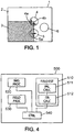
- the figure 4 illustrates a system 500 for processing a series of images captured by an image sensor adapted to implement a method according to an embodiment of the present invention.
- a system 500 may advantageously correspond to an on-board electronic card.
- circuits 510, 511, 512 may for example comprise microprocessors, programmable logic circuits such as FPGAs, ASICs or "Application-Specific Integrated Circuit” or logic integrated circuits of another type.
- circuits may for example comprise microprocessors, programmable logic circuits such as FPGAs, ASICs or "Application-Specific Integrated Circuit” or logic integrated circuits of another type.
- the steps of a method as described above are repeated, at each reiteration, they are applied by considering the following image of the previous iteration as a previous image and considering an image that follows said next image of the previous iteration as the next image.
- the figure 5a is indicative of a first source image with a group of four white rectangles and a small isolated rectangle to the right of the group.
- the figure 5b illustrates a second source image having the same group and single rectangle, the group of four rectangles being moved, relative to the first source image, by one pixel to the right of the image and two pixels down from the image and the isolated rectangle being moved two pixels down and two pixels to the right of the image.
- the figure 5c represents an estimate of the horizontal velocity field obtained following the execution of a method according to an embodiment of the present invention.
- the horizontal component of the estimated motion vectors is indicated at each point of the image by a gray level intensity value varying between white (the highest value of the horizontal component of the motion vector estimated at the point of the image considered) and black (lower value of the horizontal component of the motion vector estimated at the point of the image considered).
- figure 5d is an illustration of an estimate of the vertical velocity field obtained following the execution of a method according to an embodiment of the present invention.
- the vertical component of the estimated motion vectors is indicated at each point of the image by a gray level intensity value varying between white (the highest value of the vertical component of the motion vector estimated at the point of the image considered) and black (lower value of the vertical component of the motion vector estimated at the point of the image considered).
Description
L'invention se rapporte au domaine du traitement d'image, et plus particulièrement au domaine de l'estimation de mouvement au sein d'une séquence d'images captées.The invention relates to the field of image processing, and more particularly to the field of motion estimation within a captured image sequence.
Lorsqu'un capteur capte une séquence d'images successives, par exemple dans le cas d'une vidéo, il est connu d'effectuer une estimation de mouvement globale inter images. Cette estimation de mouvement vise à déterminer le mouvement global affectant la séquence d'images entre des couples d'images successives de la séquence et peut correspondre à la détermination du mouvement de l'axe de visée du capteur utilisé.When a sensor captures a sequence of successive images, for example in the case of a video, it is known to perform an overall motion estimation between images. This motion estimation is intended to determine the overall motion affecting the sequence of images between successive pairs of images of the sequence and may correspond to the determination of the movement of the line of sight of the sensor used.
Une telle estimation de mouvement global permet notamment la mise en oeuvre d'une stabilisation d'images, de débruitage d'images, ou encore d'algorithmes de super-résolution.Such global motion estimation makes it possible, in particular, to implement image stabilization, image denoising, or even super-resolution algorithms.
Toutefois, ce type de traitement peut être sensiblement perturbé lorsque la scène captée comprend des objets qui sont mobiles dans la scène au cours de la séquence d'images en question.However, this type of processing can be substantially disturbed when the captured scene includes objects that are movable in the scene during the sequence of images in question.
Des systèmes de traitement d'images reposent alors sur la mise en oeuvre d'une estimation de mouvement non plus globale mais dense, encore appelée « estimation de mouvement local ».Image processing systems are then based on the implementation of a motion estimation no longer global but dense, also called "local motion estimation".
Une estimation de mouvement dense consiste à estimer le mouvement en chaque point P(x,y), ou pixel, des images de la séquence captée. Plus précisément, un champ de déplacement
Outre le champ de déplacement
Les méthodes d'estimation de mouvement dense sont ainsi basées sur l'hypothèse de conservation de la luminance pour chaque point de la scène qui est traduite par l'équation de contrainte du mouvement apparent (ECMA) : ![]()
![]()
Pour déterminer le champ de vitesses ![]()

![]()
L'équation (2) peut s'écrire comme suit : ![]()
![]()
On peut enfin écrire l'équation (3) comme suit : ![]()
![]()
Afin d'estimer le vecteur de mouvement en un point P(x,y), il convient donc de résoudre cette équation (3). Cette équation ne suffit cependant pas à elle seule à déterminer le mouvement : c'est ce qui est appelé un problème « mal posé ».In order to estimate the motion vector at a point P ( x , y ), this equation (3) must be solved. This equation, however, is not enough in itself to determine the movement: it is what is called a "badly posed" problem.
Pour contourner cette difficulté, il convient d'imposer des contraintes supplémentaires sur la solution cherchée, par exemple des hypothèses de régularité locale du champ de vitesses, et différentes méthodes sont connues pour procéder à cette estimation, telles par exemple que la méthode de Horn-Schunck et la méthode de Lucas-Kanade.To circumvent this difficulty, it is necessary to impose additional constraints on the solution sought, for example hypotheses of local regularity of the velocity field, and different methods are known to make this estimation, such as for example that the method of Horn- Schunck and the Lucas-Kanade method.
Ces méthode, decrites par exemple dans
La méthode de Horn-Schunck impose une hypothèse de régularité du champ de vitesses qui limite son efficacité en présence de discontinuités du champ de vitesses. Sa résolution se fait en outre par descente de gradient et est par conséquent lente.The Horn-Schunck method imposes a hypothesis of regularity of the velocity field which limits its efficiency in the presence of discontinuities of the velocity field. Its resolution is also done by gradient descent and is therefore slow.
La méthode de Lucas-Kanade suppose la constance locale du champ de vitesses. Elle est robuste au bruit mais présente l'inconvénient d'être éparse c'est-à-dire qu'elle ne permet pas d'estimer les champs de vitesse au niveau des points dans le voisinage desquels le gradient spatial vectoriel d'intensité est uniforme localement.The Lucas-Kanade method assumes the local constancy of the velocity field. It is robust to noise but has the disadvantage of being sparse, that is to say that it does not make it possible to estimate the velocity fields at the points in the vicinity of which the intensity vector spatial gradient is locally uniform.
Par « uniforme localement », on entend que les gradients spatiaux vectoriel d'intensité au niveau des différents points du voisinage considéré sont soit sensiblement parallèles entre eux, soit sensiblement nuls. Par sensiblement nul on entend que la norme d'un gradient spatial vectoriel d'intensité considéré est inférieure au bruit de l'image.By "locally uniform" is meant that the intensity vector spatial gradients at the different points of the neighborhood considered are either substantially parallel to each other or substantially zero. By substantially zero is meant that the norm of a vector spatial gradient of intensity considered is lower than the noise of the image.
Dans la suite, on entend par gradient spatial (d'intensité) l'une quelconque des composantes scalaires (par exemple ![]()
![]()
![]()
![]()
On emploiera également de façon interchangeable l'expression « gradient spatial vectoriel d'intensité » et « gradient spatial d'intensité vectoriel ».The term "vector intensity intensity gradient" and "vector intensity spatial gradient" will also be used interchangeably.
Dans la suite, on entend par gradient spatio-temporel (d'intensité) l'une quelconque des composantes scalaires (par exemple ![]()
![]()
![]()
![]()
![]()
![]()
Il est possible de combiner les procédés de Horn-Schunck et de Lucas-Kanade, comme cela est détaillé par exemple dans l'article « Lucas/Kanade Meets Horn/Schunck: Combining Local and Global Optic Flow Methods » de A. Brunh, J. Weickert et C. Schnörr. Cette méthode présente cependant elle aussi des inconvénients tels que le coût de calcul lié à la méthode de résolution itérative utilisée dans cette méthode, ou la pondération fixe d'un terme appelé terme d'attache à la donnée qui ne tient pas compte du degré de régularité du champ de déplacement calculé.It is possible to combine the methods of Horn-Schunck and Lucas-Kanade, as detailed for example in the article "Lucas / Kanade Meets Horn / Schunck: Combining Local and Global Optic Flow Methods" by A. Brunh, J Weickert and C. Schnörr. However, this method also has disadvantages such as the calculation cost related to the iterative resolution method used in this method, or the fixed weighting of a term called attachment term to the data which does not take into account the degree of regularity of the calculated displacement field.
L'invention vise à améliorer la situation.The invention aims to improve the situation.
A cet effet, un premier aspect de l'invention propose un procédé d'estimation de mouvement dans une série d'images captées par un capteur d'image, ladite série d'images comportant au moins une image précédente I k-1 et une image suivante Ik , les images comportant des points auxquels sont associées des données d'intensité.For this purpose, a first aspect of the invention proposes a motion estimation method in a series of images captured by an image sensor, said series of images comprising at least one preceding image I k -1 and a next image I k, images with points which are associated intensity data.
Le procédé comporte une étape d'estimation de vecteurs de mouvement estimé V, réalisée en une pluralité de points d'une image choisie parmi la liste constituée par l'image précédente I k-1 et l'image suivante Ik .The method comprises an estimated motion vector estimation step V , performed at a plurality of points of an image chosen from the list consisting of the previous image I k -1 and the following image I k .
L'étape d'estimation comprend, pour chacun des points P de ladite pluralité de points d'une image, une opération de minimisation d'une fonctionnelle J de vecteurs de mouvement V.The estimation step includes, for each of the points P of said plurality of points of an image, an operation of minimizing a functional J of motion vectors V.
La fonctionnelle J comporte une somme d'au moins un terme dit terme des données et un terme dit terme de régulation.The functional J comprises a sum of at least one term term term data and a term term regulation term.
Le terme des données est fonction de gradients spatio-temporels de données d'intensité associées à une pluralité de points d'un voisinage Ω P d'un point P. Selon un mode de réalisation, le terme des données est fonction des gradients spatio-temporels vectoriels de données d'intensité associées (c'est-à-dire de chacune de leurs composantes scalaires).The term of the data is a function of spatio-temporal gradients of intensity data associated with a plurality of points of a neighborhood Ω P of a point P. According to one embodiment, the term of the data is a function of the spatial gradients. vector temporals of associated intensity data (i.e., each of their scalar components).
Le terme de régulation a une valeur finie au moins en chacun des points P de ladite pluralité de points d'une image aux niveaux desquels la minimisation du terme des données fournit une solution irrégulière.The control term has a finite value at least in each of the points P of said plurality of points of an image at which the minimization of the data term provides an irregular solution.
Une solution est irrégulière si la minimisation du terme d'attache à la donnée ne permet pas d'estimer une solution unique.A solution is irregular if the minimization of the term of attachment to the data does not make it possible to estimate a single solution.
Le terme des données comporte un produit d'un terme dit terme de pondération et d'un terme dit terme d'attache à la donnée,
le terme de pondération étant fonction d'un degré de régularité de vecteurs de mouvement V estimés,
le terme d'attache à la donnée étant fonction de gradients spatio-temporels de données d'intensité associées à une pluralité de points d'un voisinage Ω P d'un point P. Selon un mode de réalisation, le terme d'attache à la donnée est fonction des gradients spatio-temporels vectoriels de données d'intensité associées (c'est-à-dire de chacune de leurs composantes scalaires).The term data includes a product of a term called weighting term and a term term term of attachment to the data,
the weighting term being a function of a degree of regularity of estimated motion vectors V ,
the term of attachment to the datum being a function of spatio-temporal gradients of intensity data associated with a plurality of points of a neighborhood Ω P of a point P. According to one embodiment, the term of attachment to the data is a function of the vector spatio-temporal gradients of associated intensity data (that is, of each of their scalar components).
On entend ici par les termes « image précédente » et « image suivante » d'une série d'images captées, deux images qui se suivent chronologiquement dans la série d'images considérée. Ces deux images qui se suivent peuvent être consécutives (c'est-à-dire n'être séparées par aucune image captée intermédiaire) ou bien encore espacées entre elles par une ou plusieurs images captées intermédiaires. Aucune limitation n'est attachée à l'espacement entre l'image précédente et l'image suivante considérées ici.Here is meant by the terms "previous image" and "next image" of a series of captured images, two images that follow each other chronologically in the series of images considered. These two images that follow can be consecutive (that is to say, not be separated by any intermediate captured image) or else spaced apart by one or more intermediate captured images. No limitation is attached to the spacing between the previous image and the next image considered here.
On entend par les termes « estimation de vecteurs de mouvement estimé », un procédé d'estimation permettant de fournir des vecteurs de mouvements estimés pour chaque partie de l'image, avec plus ou moins de précision. Un mouvement d'image peut ainsi être estimé en chaque point de l'image par exemple. Ce type d'estimation de mouvement permet de représenter notamment le mouvement d'objets mobiles qui pourraient traverser les images de la série d'images captées. Parmi les méthodes classiques présentes dans la littérature, l'homme du métier connait notamment les méthodes de Lucas-Kanade et de Horn-Schunck.The term "estimation of estimated motion vectors" is intended to mean an estimation method making it possible to provide estimated motion vectors for each part of the image, with more or less precision. An image movement can thus be estimated at each point of the image for example. This type of motion estimation makes it possible to represent in particular the movement of moving objects that could pass through the images of the series of captured images. Among the conventional methods present in the literature, those skilled in the art know in particular the methods of Lucas-Kanade and Horn-Schunck.
Une première méthode consiste en une résolution de l'équation du mouvement apparent aux moindres carrés sur une fenêtre locale. Une deuxième méthode, extraite de l'article de Berthold K. P. Horn et Brian G. Schunck, « Determining optical flow » (ARTIFICAL INTELLIGENCE, 1981), consiste en une minimisation d'une fonctionnelle comportant un terme d'attache à la donnée comprenant le carré de l'équation du mouvement apparent, et un terme de régularisation comprenant le carré de la variation locale du champ.A first method consists in solving the equation of the least-squares motion on a local window. A second method, extracted from the article by Berthold KP Horn and Brian G. Schunck, "Determining optical flow" (ARTIFICAL INTELLIGENCE, 1981), consists of a minimization of a functional including a term of attachment to the data comprising the square of the apparent motion equation, and a regularization term including the square of the local variation of the field.
On entend par « la donnée » l'ensemble des données d'intensité des points d'une image.The term "data" refers to the set of intensity data of the points of an image.
Le « terme des données » et le « terme d'attache à la donnée ») sont des termes fonction des gradients spatio-temporels de l'intensité au niveau des points situés dans un voisinage Ω0 d'un point P 0(x 0,y 0). The "data term" and the "data term" are terms that are a function of the spatio-temporal gradients of intensity at points in a neighborhood Ω 0 of a point P 0 ( x 0 , y 0 ).
L'étendue de ce voisinage Ω0, par exemple la distance maximale des points compris dans ce voisinage par rapport au point P 0 , ainsi qu'une pondération de chacun de ces points dans un calcul de terme d'attache à la donnée peuvent être variables suivant les conditions d'utilisation du procédé.The extent of this neighborhood Ω 0 , for example the maximum distance of the points comprised in this neighborhood with respect to the point P 0 , as well as a weighting of each of these points in a calculation of term of attachment to the datum may be variables according to the conditions of use of the process.
On entend par terme de régulation, un terme ayant une valeur finie au moins en chacun des points P 0 de l'image au niveau desquels la minimisation du terme des données fourni une solution irrégulière.By regulation term is meant a term having a finite value at least in each of the points P 0 of the image at which the minimization of the term of the data provides an irregular solution.
La minimisation du terme des données fournit par exemple une solution irrégulière dans les régions homogènes et dans les régions de faible diversité angulaire. Les régions homogènes sont des régions d'intensité sensiblement constante et donc dans lesquelles les modules des gradients spatiaux vectoriels des intensités sont sensiblement nuls (inférieurs à un seuil déterminé, pouvant correspondre à un niveau de bruit). Dans une région de faible diversité angulaire les gradients spatiaux vectoriels associés d'intensité aux différents points de la région sont sensiblement parallèles.For example, the minimization of the data term provides an uneven solution in homogeneous regions and regions of low angular diversity. The homogeneous regions are regions of substantially constant intensity and therefore in which the modules of the vector spatial gradients of the intensities are substantially zero (below a determined threshold, which may correspond to a noise level). In a region of low angular diversity, the associated vector spatial gradients of intensity at different points in the region are substantially parallel.
La diversité angulaire est mesurée par exemple par la variance de l'ensemble des angles définis respectivement par une paire de gradients, pour toutes les paires de gradients possibles choisies dans l'ensemble de tous les gradients considérés.The angular diversity is measured for example by the variance of the set of angles defined respectively by a pair of gradients, for all possible pairs of gradients chosen in all of the gradients considered.
Une région de faible diversité angulaire est une région dans laquelle la diversité angulaire des gradients spatiaux d'intensité vectoriels associés aux différents points de la région est sensiblement nulle (inférieure à un seuil déterminé, pouvant correspondre à un niveau de bruit).A region of low angular diversity is a region in which the angular diversity of the vector intensity spatial gradients associated with the various points of the region is substantially zero (below a determined threshold, which may correspond to a noise level).
Une valeur finie d'un terme (par exemple un terme de régulation) est une valeur réelle ou imaginaire, unique et non infinie. Une telle valeur finie peut être définie préalablement à une étape d'estimation ou calculable au moyen d'une fonction régulière définie sur un intervalle comportant un point P 0. Un terme de régulation permet donc de lisser un champ de vecteurs de mouvement en fournissant une solution au problème consistant à minimiser une fonctionnelle aux niveaux des points d'une image où la minimisation d'un terme d'attache à la donnée ne permet pas d'estimer une solution unique.A finite value of a term (for example a regulation term) is a real or imaginary value, unique and not infinite. Such a finite value may be defined prior to an estimation step or computable by means of a regular function defined on an interval having a point P 0 . A regulation term thus makes it possible to smooth a motion vector field by providing a solution to the problem of minimizing a functional at the levels of the points of an image where the minimization of a term of attachment to the datum makes it impossible to estimate a single solution.
On entend par terme de pondération un terme permettant de pondérer l'importance relative de termes d'attache à la donnée et de termes de régulation, la pondération étant effectuée en fonction d'un gradient spatial des données d'intensité dans un voisinage d'un point P 0. Selon un mode de réalisation, la pondération est effectuée en fonction d'un gradient spatial vectoriel des données d'intensité dans un voisinage d'un point P 0.By weighting term is meant a term for weighting the relative importance of terms of attachment to the data and of regulation terms, the weighting being performed as a function of a spatial gradient of the intensity data in a neighborhood of a point P 0 . According to one embodiment, the weighting is performed according to a vector spatial gradient of the intensity data in a neighborhood of a point P 0 .
On entend par degré de régularité de vecteurs de mouvement estimé, une fonction de la variance du champ de vecteur de mouvement estimé.By estimated degree of motion vector regularity is meant a function of the variance of the estimated motion vector field.
Dans des modes de réalisation possibles de l'invention, on peut éventuellement avoir recours en outre à l'une et/ou à l'autre des dispositions suivantes :
- l'opération de minimisation est réitérée au moins une fois ;
- lors d'une itération n+1 de l'opération de minimisation, le terme de régulation comporte une fonction de vecteurs de mouvement estimé V obtenus à l'itération précédente n ;
- lors d'une itération n+1 de l'opération de minimisation, le terme de pondération comporte une fonction d'une variance locale de vecteurs de mouvement estimé V vobtenus à l'itération précédente n ;
- l'opération de minimisation de la fonctionnelle comporte une minimisation des moindres carrés ;
- le procédé comprend en outre une étape de mise à l'échelle d'images de la série d'images, ladite étape de mise à l'échelle étant réalisée préalablement à l'étape d'estimation de vecteurs de mouvement estimé V ;
- l'étape de mise à l'échelle et l'étape d'estimation sont réitérées pour au moins deux échelles différentes d'images de la série d'images ;
- le procédé comprend en outre une étape de recalage de l'image suivante Ik , réalisée après l'étape de mise à l'échelle et avant l'étape de minimisation, l'étape de recalage comprenant, pour une itération n+1 desdites étapes de mise à l'échelle, de recalage et d'estimation, le recalage de l'image suivante Ik sur la base des vecteurs de mouvement estimé V obtenus à l'itération précédente n ;
- les vecteurs de mouvement estimé V obtenus à une itération n+1 sont conservés s'ils vérifient un critère de fiabilité d'estimation et remplacé par une fonction des vecteurs de mouvement estimé V obtenus à l'itération précédente n s'ils ne vérifient pas ledit critère.
- the minimization operation is repeated at least once;
- during an iteration n + 1 of the minimization operation, the regulation term includes an estimated motion vector function V obtained at the preceding iteration n ;
- during an iteration n +1 of the minimization operation, the weighting term includes a function of a local variance of estimated motion vectors V vobtenus at the preceding iteration n ;
- the functional minimization operation includes least squares minimization;
- the method further comprises a step of scaling images of the series of images, said scaling step being performed prior to the estimation step of estimated motion vectors V ;
- the scaling step and the estimating step are repeated for at least two different scales of images in the series of images;
- the method further comprises a step of resetting the next image I k , carried out after the scaling step and before the minimization step, the resetting step comprising, for an iteration n +1 of said scaling, resetting and estimating steps, resetting the next image I k on the basis of the estimated motion vectors V obtained at the previous iteration n ;
- the estimated motion vectors V obtained at an iteration n +1 are retained if they satisfy a criterion of estimation reliability and replaced by a function of the estimated motion vectors V obtained at the previous iteration n if they do not check said criterion.
L'invention a également pour objet un système de traitement d'une série d'images captées par un capteur d'image, ladite série d'images comportant au moins une image précédente I k-1 et une image suivante Ik , les images comportant chacune des points auxquels sont associées des données d'intensité,
le système comportant un circuit d'estimation adaptée pour estimer des vecteurs de mouvement estimé V en une pluralité de points d'une image choisie parmi la liste constituée par l'image précédente I k-1 et l'image suivante Ik ,
ladite estimation comportant, pour chacun des points P de ladite pluralité de points d'une image, une opération de minimisation d'une fonctionnelle J de vecteurs de mouvement V,
la fonctionnelle J comportant une somme d'au moins un terme des données et un terme de régulation,
le terme des données étant fonction de gradients spatio-temporels de données d'intensité associées à une pluralité de points d'un voisinage Ω P d'un point P,
le terme de régulation ayant une valeur finie au moins en chacun des points P de ladite pluralité de points d'une image aux niveaux desquels la minimisation du terme des données fournit une solution irrégulière,
le terme des données comportant un produit d'un terme de pondération et d'un terme d'attache à la donnée,
le terme de pondération étant fonction d'un degré de régularité de vecteurs de mouvement V estimés,
le terme d'attache à la donnée étant fonction de gradients spatio-temporels de données d'intensité associées à une pluralité de points d'un voisinage Ω P d'un point P.The invention also relates to a system for processing a series of images captured by an image sensor, said series of images comprising at least one preceding image I k -1 and a following image I k , the images each having points with associated intensity data,
the system comprising an estimation circuit adapted to estimate estimated motion vectors V at a plurality of points of an image selected from the list constituted by the preceding image I k -1 and the following image I k,
said estimate comprising, for each of the points P of said plurality of points of an image, a minimization operation of a functional element J of motion vectors V ,
the functional J comprising a sum of at least one term of the data and a regulation term,
the term of the data being a function of spatio-temporal gradients of intensity data associated with a plurality of points of a neighborhood Ω P of a point P,
the regulation term having at least one finite value at each of the points P of said plurality of points of an image at which the minimization of the term of the data provides an irregular solution,
the term of the data comprising a product of a weighting term and a term of attachment to the datum,
the weighting term being a function of a degree of regularity of estimated motion vectors V ,
the term attachment to the data being a function of spatio-temporal gradients of intensity data associated with a plurality of points of a neighborhood Ω P of a point P.
L'invention a encore pour objet un programme d'ordinateur comprenant des instructions aptes à mettre en oeuvre un procédé tel que décrit ci-dessus, lors d'une exécution de ce programme par un circuit d'un système de traitement d'une série d'images captées par un capteur d'image.The subject of the invention is also a computer program comprising instructions able to implement a method as described above, when executing this program by a circuit of a series processing system. images captured by an image sensor.
L'invention a enfin pour objet un support d'enregistrement non transitoire sur lequel est stocké un programme d'ordinateur tel que décrit ci-dessus.The invention finally relates to a non-transitory recording medium on which is stored a computer program as described above.
D'autres caractéristiques et avantages de l'invention apparaîtront encore à la lecture de la description qui va suivre. Celle-ci est purement illustrative et doit être lue en regard des dessins annexés sur lesquels :
- la
figure 1 illustre les principales étapes d'un procédé d'estimation de mouvement selon un mode de réalisation de la présente invention ; - la
figure 2 illustre une mise en oeuvre d'un procédé d'estimation selon un mode de réalisation de la présente invention ; - la
figure 3 illustre une autre mise en oeuvre d'un procédé d'estimation selon un mode de réalisation de la présente invention ; - la
figure 4 illustre un dispositif de traitement comprenant des moyens adaptés pour mettre en oeuvre un procédé selon un mode de réalisation de la présente invention ; et - les
figures 5a, 5b, 5c et 5d illustrent respectivement une première image source, une seconde image source, une estimation du champ de vitesse horizontal obtenue suite à l'exécution d'un procédé selon un mode de réalisation de la présente invention et une estimation du champ de vitesse vertical obtenue suite à l'exécution d'un procédé selon un mode de réalisation de la présente invention.
- the
figure 1 illustrates the main steps of a motion estimation method according to an embodiment of the present invention; - the
figure 2 illustrates an implementation of an estimation method according to an embodiment of the present invention; - the
figure 3 illustrates another implementation of an estimation method according to an embodiment of the present invention; - the
figure 4 illustrates a processing device comprising means adapted to implement a method according to an embodiment of the present invention; and - the
Figures 5a, 5b, 5c and 5d respectively illustrate a first source image, a second source image, an estimation of the horizontal velocity field obtained following the execution of a method according to an embodiment of the present invention and an estimation of the vertical velocity field obtained following the carrying out a method according to an embodiment of the present invention.
De façon similaire à la méthode de Lucas-Kanade décrite dans la thèse de Bruce D. Lucas réalisée à l'université de Carnegie Mellon et publiée en 1984 sous le titre « Generalized image matching by the method of différences », le champ de vitesse peut être supposé localement constant sur un voisinage Ω0 de chaque point P 0(x 0,y0 ) . Similar to the Lucas-Kanade method described in the Bruce D. Lucas thesis done at Carnegie Mellon University and published in 1984 under the title "Generalized image matching by the method of differences", the speed field can be assumed locally constant on a neighborhood Ω 0 of each point P 0 ( x 0 , y 0 ) .
Il est alors possible de résoudre l'équation (4) par une méthode de minimisation des moindres carrés, de sorte à déterminer une valeur du champ de vitesse 
La fonction fenêtre W permet d'effectuer une pondération sur l'ensemble des points du voisinage Ω du point P 0(x 0,y 0). Elle peut par exemple être telle que ∑W = 1, par exemple W = [1 2 1]T[1 2 1]/42.The window function W makes it possible to weight on all the points of the neighborhood Ω of the point P 0 ( x 0 , y 0 ). It can for example be such that Σ W = 1, for example W = [1 2 1] T [1 2 1] / 4 2 .
Résoudre le système de l'équation (5) aux moindres carrés nécessite d'inverser une matrice de taille 2x2. Cette inversion n'est possible qu'au niveau de points présentant une diversité angulaire de gradients spatiaux de l'intensité suffisamment élevée, comme précisé ci-avant, par exemple de points dans le voisinage desquels il existe au moins deux points dont les gradients spatiaux vectoriels d'intensité lumineuse ont des directions sensiblement distinctes.Solving the system of least squares equation (5) requires inverting a 2x2 size matrix. This inversion is only possible at points having an angular diversity of spatial gradients of sufficiently high intensity, as specified above, for example points in the vicinity of which there are at least two points including spatial gradients vector of light intensity have substantially distinct directions.
Ainsi, en référence à la
Un premier voisinage 4, ayant par exemple la forme générale d'un disque centré sur l'un des sommets de la région homogène foncée 3, comprendra donc des gradients spatiaux vectoriels de l'intensité selon deux directions différentes 4a et 4b, par exemple suivant la direction horizontale et la direction verticale. Un déplacement de la région homogène foncée 3 pourra alors être complètement déterminée dans ce voisinage.A
Un deuxième voisinage 5, de forme similaire au premier voisinage 4 et situé par exemple au niveau de l'une des arrêtes verticales de la homogène foncée 3, ne comprend un gradient spatial vectoriel de l'intensité que selon une direction 5a, par exemple la direction horizontale. Le déplacement de la région homogène foncée 3 ne peut donc pas être complètement déterminé.A
Enfin, un troisième voisinage 6, également de forme similaire au premier voisinage 4, est par exemple situé en totalité dans la région homogène claire 2. Dans ce voisinage 6, le gradient spatial vectoriel de l'intensité est sensiblement nul et l'estimation du champ de déplacement est donc impossible.Finally, a
Il existe ainsi deux types de régions dans lesquelles l'estimation du champ de vitesse par une méthode de Lucas-Kanade n'est pas possible :
- les régions dans lesquelles l'intensité lumineuse est homogène (faible gradient spatial de l'intensité suivant toutes les directions) et dans lesquels il n'est donc pas possible d'estimer le champ de vitesse, et
- les régions dans lesquelles l'intensité lumineuse ne varie que suivant une direction (gradients spatiaux vectoriels de l'intensité sensiblement orientés suivant une même direction pour tous les points de la région), par exemple les bords unidimensionnels, régions dans lesquelles seule une composante du champ de vitesse n'est estimable de façon fiable.
- regions in which the luminous intensity is homogeneous (low spatial gradient of intensity in all directions) and in which it is therefore not possible to estimate the velocity field, and
- regions in which the luminous intensity varies only in one direction (vector spatial gradients of intensity substantially oriented in the same direction for all points in the region), for example the one-dimensional edges, regions in which only one component of the velocity field is estimable reliably.
Pour réaliser une minimisation en tout point, il est avantageux de minimiser la fonctionnelle J suivante en chaque point P 0(x 0,y 0) de l'image : 
Cette fonctionnelle comporte trois termes : un terme d'attache à la donnée, un terme de pondération en fonction du degré de régularité du champ estimé et un terme de régulation, qui vont maintenant être détaillés.This functional has three terms: a term of attachment to the data, a term of weighting according to the degree of regularity of the estimated field and a term of regulation, which will now be detailed.
La fonctionnelle est constituée du produit du terme de pondération et du terme de d'attache à la donnée, auquel est ajouté le terme de régulation.The functional consists of the product of the weighting term and the term of attachment to the datum, to which is added the term of regulation.
Le terme 
Le terme φ(vx ,vy ) de l'équation (6) précédente est un terme de pondération en fonction du degré de régularité du champ estimé du terme d'attache à la donnée. Ce terme permet de réduire l'importance du terme d'attache à la donnée dans les régions homogènes et unidimensionnelles.The term φ ( v x , v y ) of the preceding equation (6) is a weighting term as a function of the degree of regularity of the estimated field of the term of attachment to the datum. This term makes it possible to reduce the importance of the term of attachment to the data in the homogeneous and one-dimensional regions.
Comme détaillé ci-avant, dans les régions homogènes et unidimensionnelles, l'estimation du champ de vitesse fournie par le terme d'attache à la donnée est irrégulière et sujette à caution.As detailed above, in the homogeneous and one-dimensional regions, the estimation of the velocity field provided by the term attachment to the data is irregular and questionable.
A titre d'exemple, une fonction de la forme ϕ((var(vx ,vy )) pourra être employée pour le terme φ(vx ,vy ), la fonction étant une fonction décroissante à valeur entre 0 et 1 et var(vx ,vy ) étant la variance du champ de vitesse au point P 0(x 0,y 0) ou dans un voisinage du point P 0(x 0,y 0). Ainsi, lorsque l'estimation du champ de vitesse est irrégulière, la variance var(vx ,vy ) est élevée et le terme de pondération est proche de 0. Si, au contraire, l'estimation est régulière, la variance est faible et le terme de pondération sera proche de 1. Dans le cas où un voisinage du point P 0(x 0,y 0) est considéré, un terme de pondération φ(
A titre d'exemple, on pourra utiliser ϕ:x→1/(1+(x/0.02)2) qui est bien une fonction décroissante à valeurs entre 0 et 1.For example, we can use φ : x → 1 / (1+ ( x / 0.02) 2 ) which is a decreasing function with values between 0 and 1.
D'autres formes du terme de pondération pourront être utilisées dès qu'elles fournissent un terme de faible valeur dans les régions où l'estimation fournie par le terme d'attache à la donnée est peu fiable.Other forms of the weighting term may be used as soon as they provide a low-value term in areas where the estimate provided by the term attachment to the data is unreliable.
Le terme de pondération peut en particulier comporter un terme de pondération des régions homogènes par exemple de la forme ψ(λ +/g) où ψ est une fonction croissante positive sur [0,+∞[, λ+ est une fonction des gradients spatio-temporels de l'intensité (par exemple la valeur propre supérieure de la matrice des gradients P qui est détaillée plus loin) et g, est une valeur seuil de pondération. A titre d'exemple, on pourra utiliser une fonction ψ de la forme ψ:x→1/(1+(0.2/x)2)The weighting term can in particular include a weighting term of the homogeneous regions, for example of the form ψ ( λ + / g ) where ψ is a positive increasing function on [0, + ∞ [, λ + is a function of the spatio gradients -temporels intensity (e.g., greater eigenvalue of the matrix P gradients of which is detailed below) and g is a weighting threshold value. For example, we can use a function ψ of the form ψ : x → 1 / (1+ (0.2 / x ) 2 )
Le terme λ 2(
Le terme de régulation permet de remplacer l'estimation du champ de vitesse fournie par le terme d'attache à la donnée par la valeur moyenne dudit champ sur un voisinage du point P 0(x 0,y 0).The regulation term makes it possible to replace the estimation of the velocity field provided by the term of attachment to the datum by the average value of said field over a neighborhood of the point P 0 ( x 0 , y 0 ).
Grâce au terme de pondération détaillé ci-avant, ce remplacement est effectué uniquement au niveau des points P 0(x 0,y 0) pour lesquels ladite estimation est irrégulière par suite soit d'une absence de gradient (c'est-à-dire des gradients sensiblement nuls), soit de gradients spatiaux vectoriels sensiblement parallèles.With the weighting term detailed above, this replacement is performed only at the points P 0 ( x 0 , y 0 ) for which said estimate is irregular due either to an absence of gradient (that is, substantially zero gradients) or substantially parallel vector spatial gradients.
D'autres formes du terme de régulation pourront être utilisées, de façon à fournir un terme permettant d'obtenir une valeur du champ de vitesse cohérente avec les valeurs du champ de vitesse estimées dans le voisinage du point P 0(x 0,y 0).Other forms of the regulation term may be used, so as to provide a term for obtaining a value of the velocity field consistent with the values of the velocity field estimated in the vicinity of the point P 0 ( x 0 , y 0). ).
A titre d'exemple, les valeurs moyennes du champ de vitesse pourront être obtenues par application d'un filtre pyramidal F d'ordre 5 au champ de vitesse: 
La résolution du système est réalisée de façon itérative pour chaque point P 0(x 0,y 0) de l'image, afin d'obtenir une estimation V du champ de vitesse V = limn→+∞ Vn The resolution of the system is performed iteratively for each point P 0 ( x 0 , y 0 ) of the image, in order to obtain an estimate V of the velocity field V = lim n → + ∞ V n
A chaque itération n, la fonctionnelle des moindres carrés J au point P 0(x 0,y 0) de l'équation (6) est minimisée par une méthode matricielle. Cette méthode consiste à mettre la fonctionnelle J sous forme matricielle avant de la dériver et d'annuler cette dérivée pour obtenir une solution du champ de vitesse à l'itération n : Vn .At each iteration n , the least squares functional J at the point P 0 ( x 0 , y 0 ) of equation (6) is minimized by a matrix method. This method consists in putting the functional J in matrix form before deriving it and canceling this derivative to obtain a solution of the speed field at the iteration n : V n .
La dérivation et l'annulation de la dérivée mènent à résoudre l'équation suivante : 
![]()
![]()
![]()


![]()
![]()
![]()
Les équations définissant le terme de régularisation sont ici : 
On peut, de façon avantageuse, privilégier la régularisation non pas suivant 

Il est en outre possible de déterminer une moyenne pondérée de la direction du gradient vectoriel sur le voisinage Ω0 ce qui revient à trouver les valeurs et vecteurs propres de la matrice P.It is also possible to determine a weighted average of the direction of the vector gradient on the neighborhood Ω 0 , which amounts to finding the values and eigenvectors of the matrix P.
On peut inverser la matrice de l'équation (7) pour la résoudre et obtenir le champ de vitesse à l'itération n + 1 : ![]()


![]()
Les sommes ∑ de la matrice P peuvent être comprises comme étant des sommes sur les points Pi (xi ,yi ) du voisinage Ω0 du point P 0(x 0,y 0), et les termes W et les gradients spatio-temporels de l'intensité sont pris au niveau desdits points Pi (xi ,yi ). The sums Σ of the matrix P can be understood as being the sums of the points P i (x i, y i) of the neighborhood Ω 0 of the point P 0 (x 0, y 0), and the terms W and spatial gradients -temporal intensity are taken at said points P i ( x i , y i ) .
Les termes W correspondent à la fonction fenêtre W 0(x,y) définie ci-avant, qui permet d'effectuer une pondération sur l'ensemble des points du voisinage Ω0 du point P 0(x 0,y 0).The terms W correspond to the window function W 0 ( x , y ) defined above, which makes it possible to weight on all the points of the neighborhood Ω 0 of the point P 0 ( x 0 , y 0 ).
En référence à la
On considère ici une série d'images Ii , pour i entier compris entre 1 et N. Cette série d'images comprend au moins une image précédente Ik-1 et une image suivante Ik .We consider here a series of images I i , for i integer between 1 and N. This series of images comprises at least one previous image I k-1 and a subsequent image I k .
La première étape 100 consiste à initialiser les termes de base.The
Elle comporte une première opération 110 de calcul des dérivées spatio-temporelles de l'intensité à partir des images précédente Ik-1 et suivante Ik. Cette étape consiste donc à calculer les termes ![]()
![]()
![]()
![]()
![]()
![]()
![]()
![]()
Une deuxième opération 120 consiste à déterminer la matrice 
Au cours d'une troisième opération 130, la matrice 
Une quatrième opération 140 permet de calculer la matrice de régulation R par exemple de la façon détaillée ci-avant dans l'équation (10).A
Enfin, une cinquième opération 150 peut comporter la détermination d'un niveau de pondération des régions homogènes sur la base des valeurs propres de la matrice P. Les régions homogènes correspondent en effet aux régions dans lesquelles les valeurs propres de la matrice P sont de faibles valeurs, une valeur seuil de pondération pour les valeurs propres de la matrice P peut donc être fixée pour permettre de pondérer les régions homogènes.Finally, a
Au cours d'une deuxième étape 200, des vecteurs de mouvement sont estimés en une pluralité de points d'une image choisie parmi l'image précédente Ik-1 et l'image suivante Ik.During a
Un ensemble 201 de valeurs du champ de vitesse vx , vy en chaque point P 0(x 0,y 0) de l'image est tout d'abord initialisé. Ces valeurs correspondent au champ de vitesse V 0 à l'itération 0.A
La deuxième étape 200 comprend ensuite une première opération 210 consistant à déterminer les moyennes du champ de vitesse 
Une deuxième opération 220 va consister en un calcul du terme de pondération φ(Vn ), calcul qui peut utiliser les valeurs moyennes du champ déterminées au cours de la première opération 210 détaillée ci-avant.A
Puis, une troisième opération 230 consiste en la résolution de l'équation (10) permettant d'obtenir le nouveau champ de vitesse V n+1 de l'étape n+1 à partir des matrices déterminées au cours de l'étape préliminaire 100 ainsi que des résultats des première 210 et deuxième 220 opérations de l'étape de calcul 200.Then, a
Dans une quatrième étape 240, l'opportunité d'arrêter le calcul itératif est évaluée face à un critère prédéfini. Ce critère peut constituer à comparer le numéro n de l'itération en cours avec un nombre d'itération maximal n max, c'est-à-dire évaluer la condition n ≤ n max.In a
Dans le cas où le nombre d'itération prévu est atteint, l'étape de calcul itératif 200 se termine et retourne le dernier champ de vitesse estimé V n max.In the case where the expected iteration number is reached, the
Dans le cas contraire, le compteur du nombre d'itération n est incrémenté au cours d'une cinquième étape 250 et le champ de vitesse estimé Vn sert de valeur initiale à un nouveau calcul de l'étape 200. Il est donc utilisé comme valeur initiale pour une nouvelle opération 210 de détermination des moyennes du champ de vitesse. Les opérations suivantes 220, 230, 240 sont alors réitérées.In the opposite case, the counter of the number of iteration n is incremented during a
Un autre critère pour la quatrième étape 240 peut comprendre la comparaison d'un écart entre le champ de vitesse obtenu à l'issu de la troisième étape 230 V n+1 et le champ de vitesse obtenu à l'itération précédente Vn . A titre d'exemple un critère peut consister à évaluer la condition suivante ∥V n+1 - Vn ∥ ≤ ε où ε est une valeur prédéfinie.Another criterion for the
En se référant maintenant à la
Le développement au premier ordre (2) de l'équation de contrainte du mouvement apparent (1) détaillée ci-avant n'est valable que pour de petits déplacements, par exemple de l'ordre du pixel. Pour mesurer de grands déplacements, il est donc avantageux de procéder à un calcul multi-échelle.The first-order development (2) of the apparent motion constraint equation (1) detailed above is valid only for small displacements, for example of the order of the pixel. To measure large displacements, it is therefore advantageous to perform a multi-scale calculation.
Le procédé d'estimation de mouvement multi-échelle 400 est appliqué à une série d'images Ii , pour i entier compris entre 1 et N, cette série d'images comprenant au moins une image précédente Ik-1 et une image suivante Ik .The multi-scale
Au cours d'une première étape 410, les images précédente Ik-1 et suivante Ik sont mises à l'échelle pour donner des images mises à l'échelle Ik-1 s , Ik s . Cette étape peut comprendre l'application d'un filtre anti-repliement puis la décimation de l'image.During a
Un filtre anti-repliement est parfois dénommé aussi filtre anticrénelage ou filtre antialiasing et consiste à retirer, avant décimation les fréquences supérieures à la moitié de la fréquence de décimation. Les images pourront également être pré-filtrées pour filtrer les hautes fréquences, par exemple par des filtres pyramidaux.An anti-aliasing filter is sometimes also referred to as an anti-aliasing filter or anti-aliasing filter and consists in removing, before decimation, frequencies greater than half the decimation frequency. The images may also be pre-filtered to filter the high frequencies, for example by pyramidal filters.
Au cours d'une deuxième étape 420 et dans le cas où une première itération du procédé 400 a déjà été effectuée, une des images, par exemple l'image suivante mise à l'échelle In s est recalée en fonction du champ de déplacement Dc déterminé à l'itération précédente, pour donner une image suivante mise à l'échelle recalée In s,d .During a
Dans le cas où le procédé est à sa première itération, le champ de déplacement Dc et l'échelle Scl sont initialisé à zéro.In the case where the method is at its first iteration, the displacement field D c and the scale Scl are initialized to zero.
Une troisième étape 430 comprend l'exécution d'un procédé d'estimation de mouvement selon un mode de réalisation de la présente invention comprenant deux étapes, une étape de calculs préliminaires 100 suivie d'une étape de calcul itératif du champ de vitesse 200, tel que décrit ci-avant en relation avec la
Puis, une quatrième étape 440 de conversion du champ de vitesse résiduel V en un champ de déplacement résiduel Dr est effectuée. Cette étape peut par exemple comprendre une intégration temporelle.Then, a
Une cinquième étape 450 comprend la sommation vectorielle avec lissage du champ de déplacement résiduel Dr et du champ de déplacement Dc déterminé à l'itération précédente pour donner un champ de déplacement total Dt , au moyen de l'équation formelle suivante : ![]()
![]()
La sommation vectorielle avec lissage peut comprendre plusieurs méthodes de régularisation du champ avant ou après interpolation et sommation. Il est par exemple possible d'appliquer un filtre linéaire (par exemple un filtre pyramidal de faible taille comme celui de l'équation (11)), un filtre non-linéaire (comme une moyenne pondérée des points du voisinage), un filtrage médian ou une diffusion non-linéaire à capacité variable. Une diffusion non-linéaire à capacité variable est fondée sur une équation aux dérivées partielles similaire à l'équation de la chaleur : ![]()
![]()
La fonction c, appelée capacité, peut par exemple être de la forme c:x→1/(1+(x/k)2) où k est une capacité de filtrage, par exemple prise égale à 1 ou dépendant du niveau de bruit local. Le calcul de cette équation peut se faire par un schéma d'Euler explicite à pas fixe, le calcul du terme de divergence étant effectué par un schéma numérique de Perona-Malik.The function c , called capacitance, can for example be of the form c : x → 1 / (1+ ( x / k ) 2 ) where k is a filtering capacity, for example taken equal to 1 or depending on the noise level local. The calculation of this equation can be done by an explicit Euler scheme with fixed pitch, the calculation of the divergence term being carried out by a Perona-Malik numerical scheme.
Au cours d'une sixième étape 460, un critère de sélection est appliqué pour déterminer s'il est nécessaire de procéder à une nouvelle itération à une échelle différente. Ce critère peut par exemple être un critère fonction du champ de déplacement total Dt obtenu ou un critère fonction du nombre ou de la valeur de l'échelle Scl.In a
Dans le cas où une nouvelle itération est effectuée, une étape 470 de changement d'échelle peut être exécutée. Cette étape peut comprendre une opération de mise en forme du champ de déplacement Dc à l'itération suivante, à partir du champ de déplacement total Dt . L'étape 470 peut en outre comprendre une opération de mise à jour du paramètre d'échelle Scl à la nouvelle valeur du paramètre d'échelle.In the case where a new iteration is performed, a scaling
Un mode de réalisation alternatif du procédé d'estimation de mouvement multi-échelle 400 ci-dessus peut ne pas comprendre la deuxième étape 420 de recalage. Une estimation de champ telle que celle de la troisième étape 430 est alors réalisée à chaque échelle et le champ de déplacement final sera composé à partir des champs estimés à chaque échelle et considérés comme fiables selon un critère de conditionnement.An alternative embodiment of the multi-scale
Un tel critère de conditionnement peut par exemple être fondé sur les valeurs propres de la matrice M = φ(Vn )2 P + R détaillée dans l'équation (9) ci-avant. Cette matrice est une matrice symétrique réelle de taille 2x2 et un critère de bon conditionnement peut par exemple être fonction du rapport entre les deux valeurs propres de la matrice M, par exemple ![]()
![]()
Ainsi, pour chaque point P 0(x 0,y 0) de l'image, le champ de mouvement estimé pourra avoir soit une valeur fiable fournie par une estimation à une échelle fine soit une valeur fiable estimée à une échelle plus grossière et multipliée et zoomée par le facteur d'échelle qui convient.Thus, for each point P 0 (x 0, y 0) of the image, the estimated motion field can have either a reliable value supplied by an estimation on a fine scale is a reliable value estimated at a coarser scale and multiplied and zoomed in by the appropriate scale factor.
Une fois un procédé d'estimation exécuté, il est possible de filtrer temporellement le champ de déplacement obtenu, les objets mobiles se déplaçant usuellement avec des accélérations faibles. On peut par exemple utiliser à cette fin un filtre pyramidal d'ordre 3 sur des images recalée ou non recalées. Il est aussi possible d'utiliser un filtrage prédictif causal, c'est-à-dire prévoyant le champ de déplacement à un instant donné à partir des précédentes estimations, par exemple en supposant une vitesse de déplacement des objets mobiles dans l'image constante. Un filtrage prédictif causal permet d'estimer une donnée à partir des précédentes et d'un modèle qui peut éventuellement être ajusté. Un exemple classique est le filtrage de Kalman et l'homme du métier pourra en utiliser toute variante connue de l'état de la technique.Once an estimation method has been executed, it is possible to filter the displacement field obtained temporally, the moving objects usually moving with low accelerations. For example, it is possible to use for this purpose a pyramidal filter of
Enfin, il aussi possible d'utiliser un terme d'attache à la donnée dans le domaine fréquentiel et non pas spatial. Une telle méthode est similaire à la méthode Gabor et emploie des filtres de Gabor connus de l'homme du métier.Finally, it is also possible to use a term of attachment to the data in the frequency domain and not in the spatial domain. Such a method is similar to the Gabor method and employs Gabor filters known to those skilled in the art.
Le système d'attache à la donnée est alors le suivant : 
![]()
![]()
La
Un tel système 500 comprend :
- un
premier circuit 510 d'estimation de champ pouvant par exemple comprendre un circuit de calculs préliminaires 511 et un circuit de calcul itératif 512.
- a first
field estimation circuit 510 may, for example, comprise apreliminary calculation circuit 511 and aniterative calculation circuit 512.
Ces circuits 510, 511, 512 peuvent par exemple comprendre des micro-processeurs, des circuits logiques programmables tels que des FPGA, des ASIC ou « Application-Specific Integrated Circuit » ou des circuits intégrés logiques d'un autre type.These
Il peut en outre comprendre :
- un circuit de traitement d'images 520, adapté pour réaliser des opérations de mise à l'échelle ou de recalage d'une image.
- un circuit de traitement des
champs 530 adapté pour réaliser des opérations sur les champs de vitesse ou les champs de déplacement, par exemple la conversion d'un champ de vitesse en un champ de mouvement, la sommation vectorielle avec lissage de champs de déplacement ou le passage à l'échelle suivante. - un circuit de contrôle 540 adapté, d'une part, pour déclencher et contrôler une séquence d'étapes d'un procédé tel que décrit ci-avant en commandant les circuits d'estimation de
champ 510, de traitement d'images 520 et de traitement deschamps 530 et, d'autre part, pour décider si ledit procédé doit être réitéré et pour déclencher à nouveau la séquence si tel est le cas.
- an
image processing circuit 520, adapted to perform operations of scaling or image registration. - a suitable 530 field processing circuit to perform operations on the velocity fields or displacement fields, for example the conversion of a velocity field into a motion field, the vector summation with smoothing of displacement fields or the following scaling.
- a
control circuit 540 adapted, on the one hand, to trigger and control a sequence of steps of a method as described above by controlling thefield estimation circuit 510, theimage processing circuit 520 and the processing of thefields 530 and, secondly, to decide whether said method is to be reiterated and to re-trigger the sequence if this is the case.
Ces circuits peuvent par exemple comprendre des micro-processeurs, des circuits logiques programmables tels que des FPGA, des ASIC ou « Application-Specific Integrated Circuit » ou des circuits intégrés logiques d'un autre type.These circuits may for example comprise microprocessors, programmable logic circuits such as FPGAs, ASICs or "Application-Specific Integrated Circuit" or logic integrated circuits of another type.
Si la séquence d'étapes est déclenchée et contrôlée à nouveau, les étapes peuvent être appliquées aux mêmes images précédente et suivante.If the sequence of steps is triggered and checked again, the steps can be applied to the same previous and next images.
Dans une variante, si les étapes d'un procédé tel que décrit ci-avant sont réitérées, à chaque réitération, elles sont appliquées en considérant l'image suivante de l'itération précédente en tant qu'image précédente et en considérant une image qui suit ladite image suivante de l'itération précédente en tant qu'image suivante.$In a variant, if the steps of a method as described above are repeated, at each reiteration, they are applied by considering the following image of the previous iteration as a previous image and considering an image that follows said next image of the previous iteration as the next image.
En se référant à présent aux
La
La
La
Sur cette figure, la composante horizontale des vecteurs de mouvement estimé est indiquée en chacun des points de l'image par une valeur d'intensité de niveau de gris variant entre blanc (plus forte valeur de la composante horizontale du vecteur de mouvement estimé au point de l'image considéré) et noir (plus faible valeur de la composante horizontale du vecteur de mouvement estimé au point de l'image considéré).In this figure, the horizontal component of the estimated motion vectors is indicated at each point of the image by a gray level intensity value varying between white (the highest value of the horizontal component of the motion vector estimated at the point of the image considered) and black (lower value of the horizontal component of the motion vector estimated at the point of the image considered).
Enfin, la
Sur cette figure, la composante verticale des vecteurs de mouvement estimé est indiquée en chacun des points de l'image par une valeur d'intensité de niveau de gris variant entre blanc (plus forte valeur de la composante verticale du vecteur de mouvement estimé au point de l'image considéré) et noir (plus faible valeur de la composante verticale du vecteur de mouvement estimé au point de l'image considéré).In this figure, the vertical component of the estimated motion vectors is indicated at each point of the image by a gray level intensity value varying between white (the highest value of the vertical component of the motion vector estimated at the point of the image considered) and black (lower value of the vertical component of the motion vector estimated at the point of the image considered).
Claims (12)
- Method for estimation of motion in a series of images captured by an image sensor where said series of images comprises at least one preceding image I k-1 and one following image Ik and the images comprise points with which are associated brightness data:where said method comprises a step of estimating the estimated motion vectors, done at a plurality of image points chosen among the list made up by the previous image I k-1 and the following image Ik ;where said estimation step includes, for each of the points of said plurality of points of an image, an operation of minimization of a functional of motion vectors;where the functional comprises a sum of at least one data term and one regulation term;where the data term is a function of spatial-temporal gradients of brightness data associated with a plurality of points from a neighborhood of a point;where the regulation term has at least one finite value for each of the points of said plurality of points of an image in the area of which the minimization of the data term provides an irregular solution;said method being characterized in that the data term comprises a product of a weighting term and a data linkage term;where the weighting term is a function of the degree of regularity of the estimated motion vectors;where the data linkage term is a function of spatial-temporal gradients of brightness data associated with a plurality of points from a neighborhood of a point.
- Method according to claim 1, wherein the minimization operation is reiterated at least once.
- Method according to the preceding claim, wherein during an iteration n+1 of the minimization operation, the regulation term is a function of estimated motion vectors resulting from the preceding iteration n.
- Method according to any one of claims 2 and 3, wherein during an iteration n+1 of the minimization operation, the weighting term is a function of a local variance of estimated motion vectors resulting from the preceding iteration n.
- Method according to any one of the preceding claims, wherein the operation of minimization of the functional comprises a least-squares minimization.
- Method according to any one of the preceding claims additionally comprising a step of scaling images from the image series, where said step of scaling is done prior to the step of estimated motion vector estimation.
- Method according to claim 6, wherein the scaling step and the estimation step are iterated for at least two different image scales of the image series.
- Method according to claim 7, additionally comprising a step of registering the following image Ik , done after the scaling step and before the minimization step, where the registration step comprises, for an iteration n+1 of said scaling steps, registration and estimation steps, the registering of the following image (Ik ) over the base of estimated motion vectors resulting from the preceding iteration n.
- Method according to claim 7, wherein the estimated motion vectors resulting from an iteration n+1 are stored if they satisfy an estimation reliability criterion and replaced by a function of the estimated motion vectors resulting from the preceding iteration if they do not satisfy said criterion n.
- System for processing a series of images captured by an image sensor, where said series of images comprises at least one preceding image I k-1 and one following image Ik , where the images each comprise points with which are associated brightness data;
where the system comprises an estimation circuit suited for estimating the estimated motion vectors at a plurality of points from an image selected among the list made up by the preceding image I k-1 and the following image Ik ;
where said estimation comprises, for each of the points of said plurality of points of an image, an operation of minimization of a functional of motion vectors;
where the functional comprises a sum of at least one data term and one regulation term;
where the data term is a function of spatial-temporal gradients of brightness data associated with a plurality of points from a neighborhood of a point;
where the regulation term has at least one finite value for each of the points of said plurality of points of an image in the area of which the minimization of the data term provides an irregular solution;
where the data term comprises a product of a weighting term and a data linkage term,
where the weighting term is a function of the degree of regularity of the estimated motion vectors;
where the data linkage term is a function of spatial-temporal gradients of brightness data associated with a plurality of points from a neighborhood of a point. - Computer program comprising instructions suited for implementing a method according to any one of claims 1 to 9, during execution of this program by circuit from a system for processing a series of images captured by an image sensor.
- A medium for nonvolatile recording on which a computer program according to claim 11 is stored.
Applications Claiming Priority (2)
| Application Number | Priority Date | Filing Date | Title |
|---|---|---|---|
| FR1350271A FR3001073B1 (en) | 2013-01-11 | 2013-01-11 | MOVEMENT ESTIMATION OF AN IMAGE |
| PCT/FR2014/050049 WO2014108652A1 (en) | 2013-01-11 | 2014-01-10 | Estimation of the movement of an image |
Publications (2)
| Publication Number | Publication Date |
|---|---|
| EP2943935A1 EP2943935A1 (en) | 2015-11-18 |
| EP2943935B1 true EP2943935B1 (en) | 2017-03-08 |
Family
ID=48692571
Family Applications (1)
| Application Number | Title | Priority Date | Filing Date |
|---|---|---|---|
| EP14703136.3A Active EP2943935B1 (en) | 2013-01-11 | 2014-01-10 | Estimation of the movement of an image |
Country Status (6)
| Country | Link |
|---|---|
| US (1) | US9510013B2 (en) |
| EP (1) | EP2943935B1 (en) |
| CA (1) | CA2897674C (en) |
| FR (1) | FR3001073B1 (en) |
| IL (1) | IL239838A (en) |
| WO (1) | WO2014108652A1 (en) |
Families Citing this family (2)
| Publication number | Priority date | Publication date | Assignee | Title |
|---|---|---|---|---|
| US10499870B2 (en) * | 2017-05-19 | 2019-12-10 | The Chinese University Of Hong Kong | Methods and apparatuses for quantifying vascular fluid motions from DSA |
| US10564174B2 (en) * | 2017-09-06 | 2020-02-18 | Pixart Imaging Inc. | Optical sensing apparatuses, method, and optical detecting module capable of estimating multi-degree-of-freedom motion |
Family Cites Families (3)
| Publication number | Priority date | Publication date | Assignee | Title |
|---|---|---|---|---|
| FR2648254B2 (en) * | 1988-09-23 | 1991-08-30 | Thomson Csf | METHOD AND DEVICE FOR ESTIMATING MOTION IN A SEQUENCE OF MOVED IMAGES |
| WO2008099399A2 (en) * | 2007-02-14 | 2008-08-21 | Technion Research And Development Foundation Ltd. | Over-parameterized variational optical flow method |
| US9307251B2 (en) * | 2009-08-19 | 2016-04-05 | Sharp Laboratories Of America, Inc. | Methods and systems for determining data-adaptive weights for motion estimation in a video sequence |
-
2013
- 2013-01-11 FR FR1350271A patent/FR3001073B1/en not_active Expired - Fee Related
-
2014
- 2014-01-10 CA CA2897674A patent/CA2897674C/en active Active
- 2014-01-10 WO PCT/FR2014/050049 patent/WO2014108652A1/en active Application Filing
- 2014-01-10 EP EP14703136.3A patent/EP2943935B1/en active Active
- 2014-01-10 US US14/760,414 patent/US9510013B2/en active Active
-
2015
- 2015-07-08 IL IL239838A patent/IL239838A/en active IP Right Grant
Non-Patent Citations (1)
| Title |
|---|
| None * |
Also Published As
| Publication number | Publication date |
|---|---|
| EP2943935A1 (en) | 2015-11-18 |
| US9510013B2 (en) | 2016-11-29 |
| WO2014108652A1 (en) | 2014-07-17 |
| FR3001073A1 (en) | 2014-07-18 |
| CA2897674C (en) | 2016-07-05 |
| IL239838A (en) | 2016-11-30 |
| IL239838A0 (en) | 2015-08-31 |
| US20150358637A1 (en) | 2015-12-10 |
| CA2897674A1 (en) | 2014-07-17 |
| FR3001073B1 (en) | 2016-05-06 |
Similar Documents
| Publication | Publication Date | Title |
|---|---|---|
| EP3138079B1 (en) | Method of tracking shape in a scene observed by an asynchronous light sensor | |
| EP2795580B1 (en) | Method of estimating optical flow on the basis of an asynchronous light sensor | |
| EP1694058A1 (en) | Image capture method and device comprising local motion estimation | |
| EP3271869B1 (en) | Method for processing an asynchronous signal | |
| FR3011368A1 (en) | METHOD AND DEVICE FOR REINFORCING THE SHAPE OF THE EDGES FOR VISUAL IMPROVEMENT OF THE RENDER BASED ON DEPTH IMAGES OF A THREE-DIMENSIONAL VIDEO STREAM | |
| EP3221841A1 (en) | Method and device for the real-time adaptive filtering of noisy depth or disparity images | |
| EP2930659A1 (en) | Method for detecting points of interest in a digital image | |
| EP1746486B1 (en) | Process for detecting movement of an entity fitted with an image sensor and a device for implementing it | |
| EP1998288A1 (en) | Method for determining the movement of an entity equipped with an image sequence sensor, associated computer program, module and optical mouse. | |
| EP2943935B1 (en) | Estimation of the movement of an image | |
| EP0410826B1 (en) | Iterative motion estimation process, between a reference image and a current image, and device for canying out the process | |
| CA3105372C (en) | Processing of impulse noise in a video sequence | |
| EP1746487B1 (en) | Process and device for detection of movement of an entity fitted with an image sensor | |
| EP3072110B1 (en) | Method for estimating the movement of an object | |
| WO2019081587A1 (en) | Image restoration method | |
| FR2955007A1 (en) | ESTIMATION OF GLOBAL MOVEMENT AND DENSE | |
| Cho | Motion blur removal from photographs | |
| EP1371958A1 (en) | Method and apparatus for extracting the spectral signature of a point target | |
| WO2022233977A1 (en) | Method for processing images | |
| FR3103940A1 (en) | Image processing method and device | |
| FR3102263A1 (en) | PROCESS FOR DETERMINING THE STATE OF A SYSTEM AND DEVICE IMPLEMENTING THE SAID METHODS | |
| FR3075437A1 (en) | IMAGE SYNTHESIS METHOD | |
| FR3051066A1 (en) | METHOD FOR RESTORING IMAGES | |
| Hutchison | Signed coded exposure sequences for velocity and shape estimation from a single photo | |
| WO2015052290A1 (en) | Statistical estimation of digital image equalisation parameters |
Legal Events
| Date | Code | Title | Description |
|---|---|---|---|
| PUAI | Public reference made under article 153(3) epc to a published international application that has entered the european phase |
Free format text: ORIGINAL CODE: 0009012 |
|
| 17P | Request for examination filed |
Effective date: 20150702 |
|
| AK | Designated contracting states |
Kind code of ref document: A1 Designated state(s): AL AT BE BG CH CY CZ DE DK EE ES FI FR GB GR HR HU IE IS IT LI LT LU LV MC MK MT NL NO PL PT RO RS SE SI SK SM TR |
|
| AX | Request for extension of the european patent |
Extension state: BA ME |
|
| DAX | Request for extension of the european patent (deleted) | ||
| RAP1 | Party data changed (applicant data changed or rights of an application transferred) |
Owner name: SAFRAN ELECTRONICS & DEFENSE |
|
| RIC1 | Information provided on ipc code assigned before grant |
Ipc: H04N 19/43 20140101ALI20160719BHEP Ipc: G06T 7/20 20060101AFI20160719BHEP Ipc: H04N 5/14 20060101ALI20160719BHEP Ipc: H04N 19/513 20140101ALI20160719BHEP |
|
| GRAP | Despatch of communication of intention to grant a patent |
Free format text: ORIGINAL CODE: EPIDOSNIGR1 |
|
| INTG | Intention to grant announced |
Effective date: 20160916 |
|
| GRAS | Grant fee paid |
Free format text: ORIGINAL CODE: EPIDOSNIGR3 |
|
| GRAA | (expected) grant |
Free format text: ORIGINAL CODE: 0009210 |
|
| AK | Designated contracting states |
Kind code of ref document: B1 Designated state(s): AL AT BE BG CH CY CZ DE DK EE ES FI FR GB GR HR HU IE IS IT LI LT LU LV MC MK MT NL NO PL PT RO RS SE SI SK SM TR |
|
| REG | Reference to a national code |
Ref country code: GB Ref legal event code: FG4D Free format text: NOT ENGLISH |
|
| REG | Reference to a national code |
Ref country code: CH Ref legal event code: EP Ref country code: AT Ref legal event code: REF Ref document number: 874144 Country of ref document: AT Kind code of ref document: T Effective date: 20170315 |
|
| REG | Reference to a national code |
Ref country code: IE Ref legal event code: FG4D Free format text: LANGUAGE OF EP DOCUMENT: FRENCH |
|
| REG | Reference to a national code |
Ref country code: DE Ref legal event code: R096 Ref document number: 602014007386 Country of ref document: DE |
|
| REG | Reference to a national code |
Ref country code: NL Ref legal event code: FP |
|
| REG | Reference to a national code |
Ref country code: SE Ref legal event code: TRGR |
|
| REG | Reference to a national code |
Ref country code: LT Ref legal event code: MG4D |
|
| PG25 | Lapsed in a contracting state [announced via postgrant information from national office to epo] |
Ref country code: FI Free format text: LAPSE BECAUSE OF FAILURE TO SUBMIT A TRANSLATION OF THE DESCRIPTION OR TO PAY THE FEE WITHIN THE PRESCRIBED TIME-LIMIT Effective date: 20170308 Ref country code: GR Free format text: LAPSE BECAUSE OF FAILURE TO SUBMIT A TRANSLATION OF THE DESCRIPTION OR TO PAY THE FEE WITHIN THE PRESCRIBED TIME-LIMIT Effective date: 20170609 Ref country code: NO Free format text: LAPSE BECAUSE OF FAILURE TO SUBMIT A TRANSLATION OF THE DESCRIPTION OR TO PAY THE FEE WITHIN THE PRESCRIBED TIME-LIMIT Effective date: 20170608 Ref country code: HR Free format text: LAPSE BECAUSE OF FAILURE TO SUBMIT A TRANSLATION OF THE DESCRIPTION OR TO PAY THE FEE WITHIN THE PRESCRIBED TIME-LIMIT Effective date: 20170308 Ref country code: LT Free format text: LAPSE BECAUSE OF FAILURE TO SUBMIT A TRANSLATION OF THE DESCRIPTION OR TO PAY THE FEE WITHIN THE PRESCRIBED TIME-LIMIT Effective date: 20170308 |
|
| REG | Reference to a national code |
Ref country code: AT Ref legal event code: MK05 Ref document number: 874144 Country of ref document: AT Kind code of ref document: T Effective date: 20170308 |
|
| PG25 | Lapsed in a contracting state [announced via postgrant information from national office to epo] |
Ref country code: RS Free format text: LAPSE BECAUSE OF FAILURE TO SUBMIT A TRANSLATION OF THE DESCRIPTION OR TO PAY THE FEE WITHIN THE PRESCRIBED TIME-LIMIT Effective date: 20170308 Ref country code: LV Free format text: LAPSE BECAUSE OF FAILURE TO SUBMIT A TRANSLATION OF THE DESCRIPTION OR TO PAY THE FEE WITHIN THE PRESCRIBED TIME-LIMIT Effective date: 20170308 Ref country code: BG Free format text: LAPSE BECAUSE OF FAILURE TO SUBMIT A TRANSLATION OF THE DESCRIPTION OR TO PAY THE FEE WITHIN THE PRESCRIBED TIME-LIMIT Effective date: 20170608 Ref country code: ES Free format text: LAPSE BECAUSE OF FAILURE TO SUBMIT A TRANSLATION OF THE DESCRIPTION OR TO PAY THE FEE WITHIN THE PRESCRIBED TIME-LIMIT Effective date: 20170308 |
|
| PG25 | Lapsed in a contracting state [announced via postgrant information from national office to epo] |
Ref country code: AT Free format text: LAPSE BECAUSE OF FAILURE TO SUBMIT A TRANSLATION OF THE DESCRIPTION OR TO PAY THE FEE WITHIN THE PRESCRIBED TIME-LIMIT Effective date: 20170308 Ref country code: EE Free format text: LAPSE BECAUSE OF FAILURE TO SUBMIT A TRANSLATION OF THE DESCRIPTION OR TO PAY THE FEE WITHIN THE PRESCRIBED TIME-LIMIT Effective date: 20170308 Ref country code: SK Free format text: LAPSE BECAUSE OF FAILURE TO SUBMIT A TRANSLATION OF THE DESCRIPTION OR TO PAY THE FEE WITHIN THE PRESCRIBED TIME-LIMIT Effective date: 20170308 Ref country code: CZ Free format text: LAPSE BECAUSE OF FAILURE TO SUBMIT A TRANSLATION OF THE DESCRIPTION OR TO PAY THE FEE WITHIN THE PRESCRIBED TIME-LIMIT Effective date: 20170308 Ref country code: RO Free format text: LAPSE BECAUSE OF FAILURE TO SUBMIT A TRANSLATION OF THE DESCRIPTION OR TO PAY THE FEE WITHIN THE PRESCRIBED TIME-LIMIT Effective date: 20170308 |
|
| PG25 | Lapsed in a contracting state [announced via postgrant information from national office to epo] |
Ref country code: SM Free format text: LAPSE BECAUSE OF FAILURE TO SUBMIT A TRANSLATION OF THE DESCRIPTION OR TO PAY THE FEE WITHIN THE PRESCRIBED TIME-LIMIT Effective date: 20170308 Ref country code: IS Free format text: LAPSE BECAUSE OF FAILURE TO SUBMIT A TRANSLATION OF THE DESCRIPTION OR TO PAY THE FEE WITHIN THE PRESCRIBED TIME-LIMIT Effective date: 20170708 Ref country code: PT Free format text: LAPSE BECAUSE OF FAILURE TO SUBMIT A TRANSLATION OF THE DESCRIPTION OR TO PAY THE FEE WITHIN THE PRESCRIBED TIME-LIMIT Effective date: 20170710 Ref country code: PL Free format text: LAPSE BECAUSE OF FAILURE TO SUBMIT A TRANSLATION OF THE DESCRIPTION OR TO PAY THE FEE WITHIN THE PRESCRIBED TIME-LIMIT Effective date: 20170308 |
|
| REG | Reference to a national code |
Ref country code: DE Ref legal event code: R097 Ref document number: 602014007386 Country of ref document: DE |
|
| REG | Reference to a national code |
Ref country code: FR Ref legal event code: PLFP Year of fee payment: 5 |
|
| PLBE | No opposition filed within time limit |
Free format text: ORIGINAL CODE: 0009261 |
|
| STAA | Information on the status of an ep patent application or granted ep patent |
Free format text: STATUS: NO OPPOSITION FILED WITHIN TIME LIMIT |
|
| PG25 | Lapsed in a contracting state [announced via postgrant information from national office to epo] |
Ref country code: DK Free format text: LAPSE BECAUSE OF FAILURE TO SUBMIT A TRANSLATION OF THE DESCRIPTION OR TO PAY THE FEE WITHIN THE PRESCRIBED TIME-LIMIT Effective date: 20170308 |
|
| 26N | No opposition filed |
Effective date: 20171211 |
|
| PG25 | Lapsed in a contracting state [announced via postgrant information from national office to epo] |
Ref country code: SI Free format text: LAPSE BECAUSE OF FAILURE TO SUBMIT A TRANSLATION OF THE DESCRIPTION OR TO PAY THE FEE WITHIN THE PRESCRIBED TIME-LIMIT Effective date: 20170308 |
|
| REG | Reference to a national code |
Ref country code: CH Ref legal event code: PL |
|
| PG25 | Lapsed in a contracting state [announced via postgrant information from national office to epo] |
Ref country code: MT Free format text: LAPSE BECAUSE OF FAILURE TO SUBMIT A TRANSLATION OF THE DESCRIPTION OR TO PAY THE FEE WITHIN THE PRESCRIBED TIME-LIMIT Effective date: 20170308 |
|
| PG25 | Lapsed in a contracting state [announced via postgrant information from national office to epo] |
Ref country code: LU Free format text: LAPSE BECAUSE OF NON-PAYMENT OF DUE FEES Effective date: 20180110 |
|
| REG | Reference to a national code |
Ref country code: IE Ref legal event code: MM4A |
|
| REG | Reference to a national code |
Ref country code: BE Ref legal event code: MM Effective date: 20180131 |
|
| PG25 | Lapsed in a contracting state [announced via postgrant information from national office to epo] |
Ref country code: LI Free format text: LAPSE BECAUSE OF NON-PAYMENT OF DUE FEES Effective date: 20180131 Ref country code: CH Free format text: LAPSE BECAUSE OF NON-PAYMENT OF DUE FEES Effective date: 20180131 Ref country code: BE Free format text: LAPSE BECAUSE OF NON-PAYMENT OF DUE FEES Effective date: 20180131 |
|
| PG25 | Lapsed in a contracting state [announced via postgrant information from national office to epo] |
Ref country code: IE Free format text: LAPSE BECAUSE OF NON-PAYMENT OF DUE FEES Effective date: 20180110 |
|
| PG25 | Lapsed in a contracting state [announced via postgrant information from national office to epo] |
Ref country code: MC Free format text: LAPSE BECAUSE OF FAILURE TO SUBMIT A TRANSLATION OF THE DESCRIPTION OR TO PAY THE FEE WITHIN THE PRESCRIBED TIME-LIMIT Effective date: 20170308 |
|
| PG25 | Lapsed in a contracting state [announced via postgrant information from national office to epo] |
Ref country code: TR Free format text: LAPSE BECAUSE OF FAILURE TO SUBMIT A TRANSLATION OF THE DESCRIPTION OR TO PAY THE FEE WITHIN THE PRESCRIBED TIME-LIMIT Effective date: 20170308 |
|
| PG25 | Lapsed in a contracting state [announced via postgrant information from national office to epo] |
Ref country code: CY Free format text: LAPSE BECAUSE OF FAILURE TO SUBMIT A TRANSLATION OF THE DESCRIPTION OR TO PAY THE FEE WITHIN THE PRESCRIBED TIME-LIMIT Effective date: 20170308 Ref country code: HU Free format text: LAPSE BECAUSE OF FAILURE TO SUBMIT A TRANSLATION OF THE DESCRIPTION OR TO PAY THE FEE WITHIN THE PRESCRIBED TIME-LIMIT; INVALID AB INITIO Effective date: 20140110 Ref country code: MK Free format text: LAPSE BECAUSE OF NON-PAYMENT OF DUE FEES Effective date: 20170308 |
|
| PG25 | Lapsed in a contracting state [announced via postgrant information from national office to epo] |
Ref country code: AL Free format text: LAPSE BECAUSE OF FAILURE TO SUBMIT A TRANSLATION OF THE DESCRIPTION OR TO PAY THE FEE WITHIN THE PRESCRIBED TIME-LIMIT Effective date: 20170308 |
|
| PGFP | Annual fee paid to national office [announced via postgrant information from national office to epo] |
Ref country code: IT Payment date: 20230103 Year of fee payment: 10 Ref country code: DE Payment date: 20221220 Year of fee payment: 10 |
|
| PGFP | Annual fee paid to national office [announced via postgrant information from national office to epo] |
Ref country code: GB Payment date: 20231219 Year of fee payment: 11 |
|
| PGFP | Annual fee paid to national office [announced via postgrant information from national office to epo] |
Ref country code: SE Payment date: 20231219 Year of fee payment: 11 Ref country code: NL Payment date: 20231219 Year of fee payment: 11 Ref country code: FR Payment date: 20231219 Year of fee payment: 11 |