EP3138079B1 - Method of tracking shape in a scene observed by an asynchronous light sensor - Google Patents

Description

The present invention relates to methods for searching and tracking moving objects in scenes observed by optical sensors.

Among the known techniques for locating objects in images, there are iterative algorithms looking for the nearest points, that is to say of ICP ("Iterative Closest Point") type. These ICP algorithms are known for their efficiency in applications such as range data registration, 3D reconstruction, object tracking and motion analysis. See for example the article "Efficient Variants of the ICP Algorithm" by S. Rusinkiewicz and M. Levoy, 3rd International Lecture on 3D Digital Imaging and Modeling, June 2001, pp. 145-152 .

The principle of an ICP algorithm is to use a set of points serving as a model delimiting the object's outline in order to match it with a set of points that are part of the acquired data. A transformation between the known set-model and the set of data points is estimated to express their geometric relationships by minimizing an error function. The pursuit of an arbitrary form can be solved by an ICP technique when provided with a model of this form.

où la somme porte sur l'ensemble des points x_i du motif, est remplacée par une solution itérative dans laquelle on part d'une estimation initiale de la transformation T, et chaque itération consiste à prendre au hasard un point x_i du motif, à trouver son point correspondant y_i dans l'image et à mettre à jour la transformation T par soustraction d'un terme proportionnel au gradient ∇∥y_i - Tx_i∥² relativement aux paramètres de translation et de rotation de la transformation T. Lorsque la transformation T devient stationnaire d'une itération à l'autre, les itérations s'arrêtent et T est conservée comme estimation finale de la transformation permettant de repérer le motif dans l'image.Article "Iterative Estimation of Rigid Body Transformations - Application to Robust Object Tracking and Iterative Closest Point," by M. Hersch, et al., Journal of Mathematical Imaging and Vision, 2012, Vol. 43, No. 1, pp 1-9 , presents an iterative method for the execution of the ICP algorithm. To determine a rigid spatial transformation T making it possible to locate in an image a pattern defined by a set of points {x _i } to which correspond respectively points {y _i } of the image, the conventional solution form analytique ("closed form") , consisting in searching for the transformation T by minimizing an error criterion of the form ${\displaystyle \underset{i}{\Sigma }{\Vert {\mathrm{there}}_{\mathrm{i}}-T{\mathrm{x}}_{\mathrm{i}}\Vert }^2}$

where the sum relates to the set of points x _i of the pattern, is replaced by an iterative solution in which one starts from an initial estimate of the transformation T, and each iteration consists in taking at random a point x _i of the pattern, to find his corresponding point y _i in the image and to update the transformation T by subtraction of a term proportional to the gradient ∇∥y _i - T x _i ∥ ² relative to the translation and rotation parameters of the transformation T. When the transformation T becomes stationary from an iteration to the the other, the iterations stop and T is retained as the final estimate of the transformation for locating the pattern in the image.

In the traditional vision based on successively acquired images, the cadence of the images of the camera (of the order of 60 images per second, for example) is often insufficient for ICP techniques. Repetitive calculation of the same information in successive images also limits the real-time performance of ICP algorithms. In practice, they are confined to cases of detection of simple shapes that do not move too quickly.

Unlike conventional cameras that record successive images at regular sampling times, biological retinas transmit little redundant information on the scene to be viewed asynchronously. Asynchronous event-based vision sensors deliver compressed digital data as events. A presentation of such sensors can be found in Activity-Driven, Event-Based Vision Sensors, T. Delbrück, et al., Proceedings of 2010 IEEE International Symposium on Circuits and Systems (ISCAS), pp. 2426-2429 . Event-based vision sensors have the advantage of removing redundancy, reducing latency and increasing the dynamic range compared to conventional cameras.

The output of such a vision sensor may consist, for each pixel address, in a sequence of asynchronous events representative of changes in reflectance of the scene as they occur. Each pixel of the sensor is independent and detects changes of intensity greater than a threshold since the emission of the last event (for example a contrast of 15% on the logarithm of the intensity). When the intensity change exceeds the set threshold, an ON or OFF event is generated by the pixel as the intensity increases or decreases. Some asynchronous sensors associate detected events with light intensity measurements. Since the sensor is not sampled on a clock like a conventional camera, it can report the sequencing of events with a very high temporal accuracy (for example of the order of 1 μs). If we use such a sensor to reconstruct a sequence of images, we can achieve a frame rate of several kilohertz, against a few tens of hertz for conventional cameras.

Event-based vision sensors have promising prospects, and it is desirable to provide effective methods for tracking moving objects from signals provided by such sensors.

In "Fast sensory motor control based on event-based hybrid neuromorphic-procedural system", ISCAS 2007, New Orleans, 27-30 May 2007 pp. 845-848, T. Delbrück and P. Lichtsteiner describe a cluster tracker algorithm that can be used, for example, to control a soccer goalkeeper robot using an event-based vision sensor. Each cluster models a moving object as an event source. Events that fall in the cluster change the position of the cluster. A cluster is considered visible only if it has received a number of events greater than a threshold.

In "Asynchronous event-based visual tracking for steady haptic feedback in microrobotics", Z. Ni, et al., IEEE Transactions on Robotics, 2012, Vol. 28, No. 5, pp. 1081-1089 , it is presented an event-based version of the ICP algorithm, which is based on the minimization of a cost function in analytical form.

There is a need for a method of shape tracking that is fast and of good time accuracy.

• recevoir de l'information asynchrone d'un capteur de lumière ayant une matrice de pixels disposée en regard de la scène, l'information asynchrone comprenant, pour chaque pixel de la matrice, des événements successifs provenant dudit pixel ; et
• mettre à jour un modèle représentant la forme poursuivie d'un objet après détection d'événements attribués audit objet dans l'information asynchrone.

There is provided a method of shape tracking in a scene, comprising:

• receiving asynchronous information from a light sensor having a pixel array disposed opposite the scene, the asynchronous information comprising, for each pixel of the array, successive events from said pixel; and
• updating a model representing the continued shape of an object after detecting events attributed to said object in the asynchronous information.

• associer un point du modèle à l'événement détecté par minimisation d'un critère de distance par rapport au pixel de la matrice d'où provient l'événement détecté ; et
• déterminer le modèle mis à jour en fonction du pixel de la matrice d'où provient l'événement détecté et du point associé et indépendamment des associations effectuées avant la détection dudit événement.

The update includes, following the detection of an event:

• associating a point of the model with the detected event by minimizing a distance criterion with respect to the pixel of the matrix from which the detected event originates; and
• determining the updated model according to the pixel of the matrix from which the detected event and the associated point originates and independently of the associations made before the detection of said event.

The matching of the points observed with the model is not performed in a grouped manner after acquisition of a complete image or even of a sufficient number of events with respect to the shape pursued in the scene. The continuation of forms by the iterative algorithm is done much faster, as the asynchronous events arrive.

où:

• p[ev] désigne la position dans la matrice du pixel d'où est provenu un événement ev ;
• A[ev] désigne le point du modèle associé à l'événement ev ;
• F_t(.) désigne la transformation spatiale ;
• D(.,.) est une mesure de distance dans le plan de la matrice ;
• et la somme porte sur un certain nombre d'associations (p[ev] ↔ A[ev]) qui ont pu être effectuées.

Determining the spatial transformation for updating the model is usually based on minimizing a cost function of the form: $${\displaystyle \Sigma D\left(p\left[\mathit{ev}\right],F_t\left(\mathrm{AT}\left[\mathit{ev}\right]\right)\right)}$$

or:

• p [ev] denotes the position in the matrix of the pixel from which an ev event originated;
• A [ev] designates the point of the model associated with the event ev;
• F _t (.) Denotes spatial transformation;
• D (.,.) Is a measure of distance in the plane of the matrix;
• and the sum relates to a certain number of associations (p [ev] ↔ A [ev]) which could be carried out.

In the proposed method, the approach is different because it takes into account the association between the current event and the point of the model associated with it, but not the previous associations. While the cost function can not be minimized on this basis alone, each iteration makes it possible to compute a corrective term, in the manner of a gradient descent, which is applied to the model to converge it to the solution that continues. well shape in the scene. This convergence is ensured, even though the object is in motion, thanks to the dynamics and the high number of events that cause this movement.

To filter acquisition noise, it is possible to refrain from updating the model when no point of the model is located at a distance less than a threshold with respect to the pixel from which a detected event originates, which in this case is not attributed to the object.

• estimer un plan de déplacement de l'objet, le plan de déplacement étant estimé dans un espace à trois dimensions, à savoir deux dimensions spatiales correspondant à deux directions de la matrice de pixels et une dimension temporelle, par minimisation d'un critère de distance par rapport à un ensemble de points marquant des événements détectés qui ont été attribués à l'objet au cours d'une fenêtre temporelle se terminant à un instant courant ; et
• suite à la détection d'un événement, tenir compte du plan de déplacement estimé de l'objet pour décider d'attribuer ou non l'événement à l'objet.

An interesting embodiment of the method further comprises:

• estimate a plane of displacement of the object, the displacement plane being estimated in a three-dimensional space, namely two spatial dimensions corresponding to two directions of the pixel matrix and a temporal dimension, by minimizing a distance criterion with respect to a set of points marking detected events that have been assigned to the object during a time window ending at a current time; and
• following the detection of an event, take into account the estimated movement plan of the object to decide whether or not to attribute the event to the object.

The properties of this "displacement plane" allow several useful processes, especially in the case where several objects have respective shapes continued in the scene, each of the objects having a respective model updated after detection of events attributed to it and an estimated travel plan.

It is thus possible, following the detection of an event attributable to at least two of the objects, to calculate respective distances, in the three-dimensional space, between a point marking the detected event and the displacement planes respectively estimated for said objects. objects, and assign the detected event to the object for which the calculated distance is minimal. This makes it possible to combine spatial and temporal constraints to remove ambiguities between several objects to which a detected event is attributable.

Another possibility is to estimate a statistical distribution of distances between the plane of movement of the object and the points marking the detected events that have been attributed to the object, then, after detection of an event, take into account the plane of estimated displacement of the object and the estimated statistical distribution to decide whether or not to attribute the event to the object. This makes it possible to take into account the possible movement of the background of the scene when the asynchronous sensor is itself in motion. In particular, it is possible to determine an interval of admissible values of distance according to the estimated statistical distribution, and not assigning a detected event to the object if the point marking this event detected in the three-dimensional space has, relative to the estimated displacement plane, a distance falling outside the range of permissible values of distance.

Other features can be provided when several objects have respective shapes continued in the scene, each of the objects having a respective pattern updated after detection of events assigned to it.

Thus, if following the detection of an event, only one of the objects fulfills the condition of having in its model a point having a distance less than a threshold with respect to the pixel of the matrix from which the detected event originates, the detected event can be assigned to this object.

Following the detection of an event attributable to at least two of the objects, it is possible to take into account spatial constraints to remove the ambiguity. It is thus possible to associate with the detected event, for each object to which the detected event is attributable, a point of the model of this object by minimizing a respective distance criterion with respect to the pixel of the matrix from which the object originates. detected event, and assign the detected event to the object for which the minimized distance criterion is the lowest. An alternative is to not affect the detected event to any of the objects.

Another variant is to assign the detected event to each of the objects to which the detected event is attributable. The updating of the models of the objects to which the detected event is assigned may optionally be performed with weights depending on the distance criteria respectively minimized for said objects.

Following the detection of an event attributable to at least two objects, it is still possible to take into account temporal constraints to remove the ambiguity. For each object, it is thus possible to estimate a rate of events assigned to it and to memorize the moment at which the last event that has been assigned to it has been detected. An event attributable to at least two objects is then attributed to that of the objects for which the product of the event rate estimated by the time interval between the memorized instant and the instant of detection of the event is the highest. close to 1.

In one embodiment of the method, the determination of the updated model includes an estimate of a spatial transformation defined by a set of parameters, and an application of the estimated spatial transformation to the model. The estimation of the spatial transformation comprises a calculation of the parameters of the spatial transformation as a function of the gradient of a distance, in the plane of the pixel matrix, between the pixel of the matrix from which the detected event originates and a obtained by applying the spatial transformation to the model point associated with the detected event.

et ΔT₀ = cp - R_Δθ0 [cm], où p désigne le pixel de la matrice d'où provient l'événement détecté, m désigne le point du modèle associé à l'événement détecté, c désigne le centre de la rotation, cp désigne un vecteur allant de c à p, cm désigne un vecteur allant de c à m, et R_Δθ0 [.] est la rotation de centre c et d'angle Δθ₀.A special case is where the spatial transformation is a rigid transformation, including translation and rotation in the plane of the pixel array. One possibility is to take for translating a .DELTA.T vector equal to - η ₁ .∇ _T f (Δθ _{0, 0} .DELTA.T) and for a rotation angle Δθ equal to - η _{2 .∇} θ f (Δθ _0, DT ₀₎ where η ₁ and η ₂ are predefined positive convergence steps and Δθ ₀ and ΔT ₀ are particular values of the rotation angle and the translation vector. For example, we can take ${\mathrm{<figure-callout\; id="0"\; label="\Delta \theta "\; filenames="imgf0003.png,imgf0005.png"\; state="\{\{state\}\}">\Delta \theta </figure-callout>}}_0=\widehat{\mathit{mcp}}$

and ΔT ₀ = cp - R _{Δθ 0} [cm], where p denotes the pixel of the matrix from which the detected event originates, m denotes the point of the model associated with the detected event, c denotes the center of the rotation, cp denotes a vector ranging from c to p, cm denotes a vector ranging from c to m, and R _{Δθ 0} [.] is the rotation of center c and angle Δθ ₀ .

Another case of interest is that where the spatial transformation is an affine transformation, further including an application of respective scaling factors along two axes included in the pixel matrix. The scaling factors s _x , s _y along the two axes x, y can be calculated as s _x = 1 + η _3. (| P _x | - | m _x |) and s _y = 1 + η ₃ . | p _y | - | m _y |), respectively, where η ₃ is a predefined positive convergence step, p _x and p _y are the coordinates along the x and y axes of the matrix pixel from which the event originates detected, and m _x and m _y are the coordinates along the x and y axes of the model point associated with the detected event.

Another aspect of the present invention relates to a shape tracking device in a scene, comprising a computer configured to execute a method as defined above from asynchronous information received from a light sensor.

• la figure 1 est un schéma synoptique d'un dispositif adapté à la mise en oeuvre de l'invention ;
• la figure 2A est un diagramme montrant un exemple de profil d'intensité lumineuse au niveau d'un pixel d'un capteur asynchrone ;
• la figure 2B montre un exemple de signal délivré par le capteur asynchrone en réponse au profil intensité de la figure 2A ;
• la figure 2C illustre la reconstruction du profil intensité à partir du signal de la figure 2B ;
• les figures 3A-B sont des diagrammes analogues à ceux des figures 2A-B illustrant un mode d'acquisition lumineuse utilisable dans un autre exemple de réalisation du procédé ;
• la figure 4 est un schéma synoptique d'un capteur asynchrone de lumière de type ATIS ;
• la figure 5 est un diagramme montrant des événements générés par un capteur asynchrone placé en regard d'une scène comportant une étoile tournante ;
• la figure 6A et une vue d'un équipement utilisé pour tester le fonctionnement du procédé de poursuite de forme selon l'invention ;
• la figure 6B montre un exemple de carte d'accumulation d'événements obtenue dans la configuration de la figure 5A ;
• la figure 7 montre différentes images pour illustrer le fonctionnement d'un algorithme ICP dans l'exemple d'une étoile tournante ;
• la figure 8 est un organigramme d'un exemple d'algorithme qui ne représente pas un mode de réalisation de l'invention ;
• les figures 9 et 10 sont des diagrammes montrant des éléments géométriques - la figure 9 ne représente pas un mode de réalisation de l'invention ;
• la figure 11 est un organigramme d'un exemple d'algorithme utilisable dans d'autres mises en oeuvre de l'invention ;
• la figure 12 est un diagramme illustrant un mode de calcul de transformation spatiale lors d'une itération d'un mode de réalisation d'un procédé selon la figure 11;
• la figure 13 est un graphique montrant les points d'un espace à trois dimensions, incluant deux dimensions spatiales et une dimension temporelle, où sont enregistrés les événements attribués à une arête en mouvement dans le champ de vision d'un capteur asynchrone, et leur interpolation par un plan de déplacement ;
• la figure 14 est un organigramme d'un exemple de procédure utilisable à l'étape 44 de la figure 11 ;
• les figures 15 et 16 sont des organigrammes d'exemples de procédures utilisables à l'étape 56 de la figure 14 ;
• la figure 17 est un graphique montrant une distribution de distances entre des événements et un plan de déplacement du type de celui montré sur la figure 13 ;
• la figure 18 est un organigramme d'une procédure utilisable pour estimer un intervalle de valeurs admissibles de distance tel que représenté sur la figure 17 ;
• la figure 19 est un graphique indiquant des erreurs de poursuite constatées en appliquant trois méthodes de poursuite différentes dans une expérience réalisée dans les conditions des figures 6 et 7 ;
• la figure 20 est un diagramme illustrant la poursuite de trois formes d'objets dans un exemple d'exécution de l'invention ;
• la figure 21 est un graphique illustrant les résultats d'une expérience réalisée en prenant en compte des facteurs d'échelle s_x, s_y dans la transformation spatiale appliquée au modèle d'un objet dans une réalisation de l'invention ;
• la figure 22 montre des images obtenues dans une autre expérimentation de l'invention ;
• les figures 23 et 24 sont des graphiques indiquant des erreurs de poursuite constatées en appliquant deux méthodes de poursuite différentes dans l'expérimentation de la figure 22 ;
• les figures 25 et 26 sont des graphiques illustrant deux mode possibles de levée d'ambiguïté entre plusieurs objets dans une autre expérimentation de l'invention ;
• les figure 27-32 sont des graphiques indiquant les vitesses de modèles observés lors de la poursuite de deux formes d'objets en mouvement selon six méthodes différentes dans la même expérimentation que les figures 25-26 ;
• la figure 33 est un graphique montrant deux plans de déplacement suivant la figure 13, utilisés pour décider de l'attribution d'événements aux objets dans le cadre de la poursuite dans les résultats sont montrés sur la figure 32 ; et
• les figure 34 et 35 sont des graphiques montrant des vitesses de modèle obtenues dans deux expérimentations de l'invention dans lesquelles le capteur asynchrone était lui-même en mouvement.

Other features and advantages of the present invention will appear in the description below, with reference to the accompanying drawings, in which:

• the figure 1 is a block diagram of a device adapted to the implementation of the invention;
• the Figure 2A is a diagram showing an example of a light intensity profile at a pixel of an asynchronous sensor;
• the Figure 2B shows an example of signal delivered by the asynchronous sensor in response to the intensity profile of the Figure 2A ;
• the Figure 2C illustrates the reconstruction of the intensity profile from the signal of the Figure 2B ;
• the Figures 3A-B are diagrams similar to those of Figures 2A-B illustrating a light acquisition mode that can be used in another embodiment of the method;
• the figure 4 is a block diagram of an asynchronous ATIS type light sensor;
• the figure 5 is a diagram showing events generated by an asynchronous sensor placed next to a rotating star scene;
• the Figure 6A and a view of equipment used to test the operation of the shape tracking method according to the invention;
• the Figure 6B shows an example of event accumulation map obtained in the configuration of the Figure 5A ;
• the figure 7 shows different images to illustrate the operation of an ICP algorithm in the example of a rotating star;
• the figure 8 is a flowchart of an exemplary algorithm that does not represent an embodiment of the invention;
• the Figures 9 and 10 are diagrams showing geometric elements - the figure 9 does not represent an embodiment of the invention;
• the figure 11 is a flowchart of an exemplary algorithm that can be used in other implementations of the invention;
• the figure 12 is a diagram illustrating a spatial transformation calculation mode during an iteration of an embodiment of a method according to the figure 11 ;
• the figure 13 is a graph showing the points of a three-dimensional space, including two spatial dimensions and one time dimension, where the events assigned to a moving edge in the field of view of an asynchronous sensor are recorded, and their interpolation by a travel plan;
• the figure 14 is a flowchart of an example of procedure usable at step 44 of the figure 11 ;
• the figures 15 and 16 are flowcharts of examples of procedures usable at step 56 of the figure 14 ;
• the figure 17 is a graph showing a distance distribution between events and a displacement plane of the type shown on the figure 13 ;
• the figure 18 is a flowchart of a procedure that can be used to estimate an interval of allowable range values as shown on the figure 17 ;
• the figure 19 is a graph showing tracking errors found by applying three different tracking methods in an experiment conducted under Figures 6 and 7 ;
• the figure 20 is a diagram illustrating the continuation of three forms of objects in an exemplary embodiment of the invention;
• the figure 21 is a graph illustrating the results of an experiment performed by taking into account scaling factors s _x , s _y in the spatial transformation applied to the model of an object in one embodiment of the invention;
• the figure 22 shows images obtained in another experiment of the invention;
• the figures 23 and 24 are graphs indicating tracking errors found by applying two different tracking methods in the experimentation of the figure 22 ;
• the Figures 25 and 26 are graphs illustrating two possible ways of removing ambiguity between several objects in another experiment of the invention;
• the Figure 27-32 are graphs showing model speeds observed when tracking two moving object shapes using six different methods in the same experiment as the Figures 25-26 ;
• the figure 33 is a graph showing two planes of displacement following the figure 13 , used to decide the assignment of events to objects as part of the pursuit in the results are shown on the figure 32 ; and
• the figure 34 and 35 are graphs showing model speeds obtained in two experiments of the invention in which the asynchronous sensor was itself in motion.

The device represented on the figure 1 comprises an event-based asynchronous vision sensor 10 placed facing a scene and receiving the light flux of the scene through an acquisition optics 15 comprising one or more lenses. The sensor 10 is placed in the image plane of the acquisition optics 15. It comprises a group of photosensitive elements organized in a matrix of pixels. Each pixel corresponding to a photosensitive element produces successive events depending on the variations of light in the scene.

A computer 20 processes the asynchronous information from the sensor 10, that is to say the event sequences ev (p, t) received asynchronously from the different pixels p, to extract information F _t from some forms evolving in the scene. The computer 20 operates on digital signals. It can be implemented by programming an appropriate processor. A hardware implementation of the computer 20 using specialized logic circuits (ASIC, FPGA, etc.) is also possible.

For each pixel p of the array, the sensor 10 generates an event-based asynchronous signal sequence from the light variations felt by the pixel in the scene appearing in the field of view of the sensor.

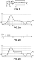
The asynchronous sensor makes an acquisition for example according to the principle illustrated by the Figures 2A-C . The information delivered by the sensor comprises a succession of instants t _k (k = 0, 1, 2, ...) at which an activation threshold Q is reached. The Figure 2A shows an example of a light intensity profile P1 seen by a pixel of the sensor matrix. Whenever this intensity increases by an amount equal to the activation threshold Q from what it was at time t _k , a new moment t _{k + 1} is identified and a positive line (level +1 on the Figure 2B ) is issued at this time t _{k + 1} . Symmetrically, each time the intensity of the pixel decreases by the quantity Q from what it was at time t _k , a new moment t _{k + 1} is identified and a negative line (level -1 on the Figure 2B ) is issued at this time t _{k + 1} . The asynchronous signal sequence for the pixel then consists of a succession of positive or negative pulses or lines ("spikes") positioned in time at times t _k depending on the light profile for the pixel. These lines can be represented mathematically by Dirac peaks positive or negative and each characterized by a transmission instant t _k and a sign bit. The output of the sensor 10 is then in the form of an address-event representation (AER). The Figure 2C shows the intensity profile P2 that we are able to reconstruct as an approximation of the profile P1 by integration in time of the asynchronous signal of the Figure 2B .

The activation threshold Q can be fixed, as in the case of Figures 2A-C , or adaptive depending on the light intensity, as in the case of Figures 3A-B . For example, the threshold ± Q can be compared to changes in the logarithm of light intensity for the generation of an event ± 1.

For example, the sensor 10 may be a dynamic vision sensor (DVS) of the kind described in "At 128x128 120 dB 15 μs Latency Asynchronous Temporal Contrast Vision Sensor," P. Lichtsteiner, et al., IEEE Journal of Solid-State Circuits, Vol. 43, No. 2, February 2008, pp. 566-576 , or in the patent application US 2008/0135731 A1 . The dynamics of a retina (minimum duration between action potentials) of the order of a few milliseconds can be approximated with a DVS of this type. The performance in dynamics is in any case much greater than that which can be achieved with a conventional video camera having a realistic sampling frequency. It should be noted that the form of the asynchronous signal delivered for a pixel by the DVS 10, which constitutes the input signal of the computer 20, may be different from a succession of Dirac peaks, the events represented being able to have a width any amplitude or waveform in this asynchronous event-based signal.

Another example of an asynchronous sensor advantageously usable in the context of the present invention is the time-based asynchronous time-based image sensor (ATIS), a description of which is given in the article. A QVGA 143 dB Dynamic Range Frame-Free PWM Image Sensor with Lossless Pixel-Level Compression Video and Time-Domain CDS, C. Posch, et al., IEEE Journal of Solid-State Circuits, Vol. 46, No. 1, January 2011, pp. 259-275 .

The figure 4 illustrates the principle of ATIS. A pixel 16 of the matrix constituting the sensor comprises two photosensitive elements 17a, 17b, such as photodiodes, respectively associated with electronic detection circuits 18a, 18b. The sensor 17a and its circuit 18a have a similar operation to those of the previously mentioned DVS. They produce a pulse P ₀ when the light intensity received by the photodiode 17a varies by a predefined quantity. The pulse P ₀ marking this intensity change triggers the electronic circuit 18b associated with the other photodiode 17b. This circuit 18b then generates a first pulse P ₁ then a second pulse P _{2 as} soon as a given amount of light (number of photons) is received by the photodiode 17b. The time difference δt between the pulses P ₁ and P ₂ is inversely proportional to the light intensity received by the pixel 16 just after the appearance of the pulse P ₀ . Asynchronous information from the ATIS is another form of AER representation, comprising two pulse trains for each pixel: the first pulse train P ₀ indicates the times when the light intensity has changed beyond the detection threshold, while the second train consists of pulses P ₁ and P ₂ whose time difference δt indicates the corresponding light intensities, or gray levels. An event ev (p, t) coming from a pixel 16 of position p in the matrix of the ATIS then comprises two types of information: a temporal information given by the position of the pulse P ₀ , giving the instant t of the event, and a gray level information given by the time difference δt between the pulses P ₁ and P ₂ .

par le mouvement d'une étoile tournant à vitesse angulaire constante comme schématisé dans l'encadré A. La majeure partie de ces points se répartissent à proximité d'une surface de forme générale hélicoïdale. En outre, la figure montre un certain nombre d'événements à distance de la surface hélicoïdale qui sont mesurés sans correspondre au mouvement effectif de l'étoile. Ces événements sont du bruit d'acquisition.In the case where the sensor 10 consists of a two-dimensional array of pixels, the events from the pixels can be placed in a three-dimensional space-time representation such as that presented on FIG. figure 5 . In this figure, each point identifies an event ev (p, t) generated asynchronously at a time t at a pixel p of the sensor, of position $p=\left(\begin{array}{c}x\\ \mathrm{there}\end{array}\right),$

by the motion of a star rotating at constant angular velocity as shown schematically in Box A. The majority of these points are distributed near a surface of helical general shape. In addition, the figure shows a number of events at a distance from the helical surface that are measured without corresponding to the actual motion of the star. These events are acquisition noise.

The principle of an ICP algorithm is to use a set of points forming a model representing the shape of an object, for example describing the outline of this object, to match it with a set of points provided by data of acquisition, then calculate the geometric relation between this set of points and the model by minimizing an error function.

The Figure 6A shows the equipment used in an experiment of the invention, the sensor 10, for example DVS or ATIS type, being placed in front of a turntable 11 on which is designed a star shape. The sensor 10 acquires data from the rotation of the star shape on the tray. By way of comparison and illustration, the Figure 6B shows schematically the events observed during a time interval of the order of a few microseconds, superimposed on the black form of the star.

The figure 7 shows, by way of illustration, an example of continuation of the star shape. In this figure, the top row is a conventional image sequence showing the star in rotation on its plateau, as in the case of the Figure 6A . The middle row shows event accumulation maps, i.e., the projection of all events occurring over a period of time on a plane, regardless of the precise times of event detection in the period of time. Finally, the bottom row shows the matching of the model (shown in solid lines) with the acquisition points. In the left column (a), we see an initial state where the star begins its rotation. The algorithm tries to match the model with the nearest events. An initial position of the model not too far from the events is useful for the algorithm to converge towards the global minimum. In column (b), the star goes to near the initial position of the model, and this converges towards the position of the star. Finally, in columns (c) and (d), the star continues to rotate and the model is updated by applying a rotation R _Δθ and a translation ΔT whose parameters are calculated by minimizing an error function.

In the case where the scene is observed by an event-based asynchronous sensor rather than a conventional camera, events are received with accurate dating as they occur. An ICP-type algorithm does not need to wait for information on the entire scope of the scene to handle all the events it contains simultaneously.

où Δt est un temps de persistance. Après que l'intervalle de temps Δt s'est écoulé suite à l'activation d'un événement, cet événement est éliminé de l'ensemble S(t).An event ev (p, t) describes an activity in the spatio-temporal domain. In the event-based version of the ICP algorithm illustrated on the figure 8 it is considered, in a similar way to biological neurons, that each event has an influence for a certain period of time after its appearance. This temporal property of events can be introduced as a persistence function. We then denote S (t) the spatio-temporal set of events that are active at a time t: $$\mathrm{S}\left(\mathrm{t}\right)=\left\{\mathrm{ev}\left(\mathrm{p},\mathrm{t}\text{'}\right)/0<\mathrm{t}-\mathrm{t}\text{'}\le \mathrm{.delta.t}\right\}$$

where Δt is a persistence time. After the time interval Δt has elapsed following the activation of an event, this event is eliminated from the set S (t).

Matching the points between the model and the acquisition data is the most demanding step in computing resources. We denote G (t) the set of positions of the points of the two-dimensional model defining the shape of the object at a time t. The association between the acquisition points and the points of the model can be performed sequentially. Each time a new event is activated, it is mapped to an element of G (t), preferably to an element of G (t) that has not already been associated with an event of S (t). We can add at this step the verification of a distance criterion to reject noise or other points that are not part of the desired form.

Since the sensor is asynchronous, the number of associated points varies quite strongly. There are typically a few points to a few hundred associated points during the persistence time Δt. This is very different from the conventional frame-based approach. Stationary objects do not generate any stimulus so there is no need to update their position. When the scene has little movement, only a small amount of compute resources are used, whereas in highly dynamic situations the algorithm requires its full capacity to update the information.

In the example of the figure 8 , we denote by P (n) and T (n) the position and the detection time of the nth event retained for updating the position information of the model, and M (n) the point of the model associated with this n -th event. The detection times T (n) are initialized to arbitrarily large values before starting the algorithm (T (n) = + ∞). When detecting an event ev (p, t) at time t, the integer index a designates the oldest event in S (t) while the integer index b designates the most recent event in S (t), that is S (t) = {ev (P (a), T (a)), ev (P (a + 1), T (a + 1)), ..., ev (P ( b), T (b))}. The model G (t) is simply denoted by G, and we denote by M the set of points of the model which have been associated with the events of S (t), ie M = {M (a), M (a + 1), ..., M (b)}. At initialization of the algorithm (step 20), the integer indexes a and b are respectively initialized to 1 and to 0.

In the version of the algorithm shown on the figure 8 , the spatial transformation F _t which corresponds the points of the model to the positions of the detected events is periodically estimated, by a conventional solution in analytical form, for example by singular value decomposition (SVD). In step 21, the algorithm waits for new events from the sensor 10 until the update period of the spatial transformation has elapsed.

Following receipt of an event ev (p, t) coming from a pixel of position p in the matrix at time t (step 22), two operations are performed: update of the set S (t) and association with the detected event of a model G point. In the loop 23-24, events dating more than Δt are eliminated from S (t): the test 23 looks at whether the time T (a) is greater than at t - Δt. If T (a) is not greater than t - Δt, the number a is incremented by one unit in step 24 and the test 23 is reiterated. Events that are too old are eliminated when T (a)> t - Δt on test 23.

The algorithm then proceeds to associate a point of G with the new event in step 25. This associated point is the one whose position m is closest to the pixel p from which the event ev (p , t) among the points in the model that have not already been associated with a point of the set S (t), that is, among the points of the set GM: $$m=\underset{q\in \mathrm{BOY\; WUT}-M}{\mathit{Arg}\min }\left[d\left(p,q\right)\right]$$

The distance criterion d (.,.) Used at this step 25 is for example the Euclidean distance in the plane of the matrix. Before deciding whether the event ev (p, t) will be included in the set S (t), the algorithm examines in step 26 whether the minimized distance is less than a threshold d _max . For example, we can choose the threshold d _max as corresponding to 6 pixels. A different threshold value can naturally be used if tests show that it is better for a particular application. If d (p, m) ≥ d _max , the event is discarded and the algorithm returns to step 21 waiting for the next event.

If the event is assigned to the sought object (d (p, m) <d _max in test 26), the index b is incremented by one unit in step 27, then the detection time t, the position p of this event and the point m of the model which has just been associated with it are recorded as T (b), P (b) and M (b) in step 28. The processing following the detection of the Event ev (p, t) is then completed and the algorithm returns to step 21 waiting for the next event.

At the expiration of the update period of the spatial transformation, a test is performed to ensure that a sufficient number of events are in the set S (t) to contribute to the update. , for example L = 5 events. Thus, if b <a + L - 1 (test 30), no update is performed and the algorithm returns to step 21 waiting for the next event.

If there are enough events (b ≥ a + L - 1), a minimization operation 31 is performed to choose a rotation angle Δθ and a vector of ΔT translation in the case where the spatial transformation F _t , which one looks for from the model G, is the combination of a rotation R _Δθ of angle Δθ and a translation of vector ΔT.

The figure 9 specifies the notation used here. We denote H the point pattern defining the shape pursued in the scene, placed at a fixed position, and O the center of gravity of this set of points H. At a time t, this pattern H has moved in a translation of vector T and a rotation angle θ around its center of gravity O, which gives the model G = G (t) to which reference is made when processing a received event at time t. The treatment gives rise to the estimation of variations Δθ, ΔT of the rotation angle θ and of the translation vector T.

qui est un cas particulier de l'expression (1) où les paramètres à estimer sont l'angle Δθ de la rotation R_Δθ, définie par la matrice $R_{\mathrm{\Delta }\theta }=\left[\begin{array}{cc}\cos \mathrm{\Delta }\theta & -\sin \mathrm{\Delta }\theta \\ \sin \mathrm{\Delta }\theta & \cos \mathrm{\Delta }\theta \end{array}\right],$

et les coordonnées du vecteur ΔT. Dans l'expression (4), les notations cP(n) et cM(n) représentent les vecteurs ayant pour origine le centre c de la rotation R_Δθ et pointant respectivement vers P(n) et M(n). La position du centre c de la rotation R_Δθ peut être définie par rapport au modèle G(t). Par exemple, on peut placer le point c au centre de gravité des points du modèle G(t), comme représenté sur la figure 9 (le vecteur T de la translation globale est alors égal au vecteur Oc).The minimization operation 31 consists in finding the parameters Δθ, ΔT which minimize a distance criterion such as for example a sum of the form: $${{\displaystyle \underset{\mathrm{not}=\mathrm{at}}{\overset{b}{\Sigma }}\Vert \mathit{cP}\left(\mathrm{not}\right)-R_{\mathrm{\Delta }\theta }\left[\mathit{cM}\left(\mathrm{not}\right)\right]-\mathrm{\Delta }T\Vert }}^2$$

which is a particular case of the expression (1) where the parameters to be estimated are the angle Δθ of the rotation R _Δθ , defined by the matrix $R_{\mathrm{\Delta }\theta }=\left[\begin{array}{cc}\cos \mathrm{\Delta }\theta & -\sin \mathrm{\Delta }\theta \\ \sin \mathrm{\Delta }\theta & \cos \mathrm{\Delta }\theta \end{array}\right],$

and the coordinates of the vector ΔT. In expression (4), the notation cP (n) and cM (n) represent vectors originating from the center c of the rotation R _Δθ and pointing respectively to P (n) and M (n). The position of the center c of the rotation R _Δθ can be defined with respect to the model G (t). For example, we can place the point c at the center of gravity of the points of the model G (t), as represented on the figure 9 (The vector T of the global translation is then equal to the vector Oc).

The spatial transformation F _t composed of the rotation R _Δθ and the translation ΔT is here the one that moves the model G (t) to bring it closer to the pixels in which events recently taken into account have been detected. ie events of the set S (t). This is what the figure 10 , where the + signs represent the positions of the pixels P (n) where the events of S (t) have been detected, the signs • represent the positions of the points M (n) of the model G that have been associated with these events, and BOY WUT' represents the next model, of center c ', which places the points M (n) as close as possible to the pixels P (n) and results from a displacement of G according to the rotation R _Δθ and the vector translation ΔT.

The rotation R _Δθ and the translation ΔT which minimize the criterion (4) translate the movement of the form corresponding to the model G between the update time of the spatial transformation and the previous update time. In step 32, the same transformation is applied to the points of the sets G and M to update these two sets. Each position X of the model G (or of the set M) is replaced by a position Y such that cY = R _Δθ [cX] + ΔT. After this step 32, the algorithm returns to step 21 waiting for the next event.

The spatial transformations F _t thus characterized by the angles Δθ of successively estimated rotations R _Δθ and by the corresponding translation vectors ΔT represent the movements of the shape pursued in the scene. Their parameters are the outputs of the calculator 20 of the figure 1 . It is possible to accumulate the values Δθ and ΔT successively determined to obtain the angles θ and the translation vectors T defined with respect to the fixed reference position of the form H.

The embodiment illustrated by the figure 8 to control the update rate of the tracking information of the shape sought in the scene, i.e. parameters of the spatial transformation F _t . Typically, this update frequency corresponds to a periodicity of between 10 μs and 1 ms. It can therefore be much faster than the frame frequencies of conventional cameras.

The persistence time Δt is set according to the dynamic content of the scene. In an implementation based on SVD calculations, it is desirable that the time interval Δt be long enough for the set S (t) to keep a complete contour of the desired moving object, so that almost all the points of contour can be mapped to events. On the other hand, a too long duration Δt increases the computational load, and does not allow to pursue fast objects. The duration Δt is typically chosen between 10 μs and 20 ms.

Another approach to the shape continuation in the scene seen by the asynchronous sensor 10 is illustrated by the figure 11 . In this approach, which provides a better dynamic while requiring less computation, the spatial transformation F _t which makes it possible to update the updated model is determined according to the pixel p of the matrix from which a detected event ev (p, t) (as long as this event has been assigned to the searched object) and the associated point m, independently of the associations made before detecting the event ev (p, t).

In the representation of the figure 11 , we consider that a number K of objects are searched in the scene observed by the asynchronous sensor. These objects are numbered by an integer k (k = 1, 2, ..., K), and each has a model of points denoted G _k (t) or simply G _k . The frequent case where a single object is pursued is included taking K = 1.

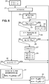
To initiate the tracking of each object k, its model G _k is initialized (step 40) with a positioning quite close to that of this object in the field of view of the sensor 10. Then, in step 41, the algorithm waits new events from the sensor 10.

Following receipt of an event ev (p, t) from a pixel of position p in the matrix at time t (step 42), a step 43 of association of a point m _k of the model G _k to the detected event is performed for each object k (k = 1, 2, ..., K). For each object k, this step 43 is identical to the step 25 previously described with reference to FIG. figure 8 , except that the point m _k of the model G _k which minimizes the distance criterion d (m _k , p) is chosen without excluding points previously associated with events, the algorithm not memorizing the associations prior to the event. event ev (p, t).

In step 44, the event ev (p, t) that was detected in step 42 is assigned to an object k or, failing that, excluded as not related to the movement of an object pursued in the scene. If the event ev (p, t) is not assigned to any object, the algorithm returns to step 41 waiting for the next event. In case of assignment to an object k, the spatial transformation F _t is calculated in step 45 for the model G _k of this object.

Several tests or filtering can be performed in step 44 to make the decision whether or not to assign the event ev (p, t) to an object k.

The simplest is to proceed as in step 26 described above with reference to the figure 8 by comparing the distance d (m _k , p) to a threshold d _max . If d (m _k , p) <d _max , the association of the pixel p to the point m _k of the model G _k is confirmed, and if no object fulfills this condition, no attribution is made. It is possible, however, that several objects pursued fulfill this condition, one being capable of obscuring the other. To solve these ambiguous cases, including cases of occlusion between objects, several techniques are applicable, using either spatial constraints or temporal constraints. These techniques will be discussed later.

Another treatment that may occur in step 44 is taking into account the possible movement of the bottom. In particular, if the asynchronous sensor 10 is itself in motion, the fixed bottom is in relative displacement and generates the detection of numerous events that are to be excluded from the processes relating to the pursuit of the objects of interest. One way to take into account the movement of the bottom will be described later.

Once the event ev (p, t) has been assigned to an object k, the parameters of the spatial transformation F _t are calculated at step 45 and this transformation F _t is applied to the model G _k to update this at step 46. Finally, a displacement plane of the object k, noted Π _k , is estimated at step 47. The algorithm then returns to step 41 waiting for the next event.

où d[., .] est une mesure de distance dans le plan de la matrice de pixels. Cela peut notamment être une distance quadratique.Limiting to a current event p associated with a point m of the model G _k to calculate a spatial transformation F _t leads to introducing a function component cost f: $$\mathrm{f}=\mathrm{d}\left[\mathrm{p},{\mathrm{F}}_{\mathrm{t}}\left(\mathrm{m}\right)\right]$$

where d [.,.] is a measure of distance in the plane of the pixel matrix. This can be a quadratic distance.

où cp et cm désignent les vecteurs ayant pour origine le centre c de la rotation R_Δθ et pointant respectivement vers les points p et m.If one considers rigid spatial transformations for the update of the model G _k , it is necessary to determine the angle Δθ of a given rotation R _Δθ of center c and the vector ΔT of a translation, the component of cost function with a quadratic distance is written: $$f={\Vert \mathit{cp}-R_{\mathrm{\Delta }\theta }\left[\mathit{cm}\right]-\mathrm{\Delta }T\Vert }^2$$

where cp and cm denote the vectors originating from the center c of the rotation R _Δθ and pointing respectively to the points p and m.

$$\mathrm{\Delta \theta }={\mathrm{\eta }}_2.{\nabla }_{\mathrm{\theta }}\mathrm{f}\left({\mathrm{\Delta \theta }}_0,{\mathrm{\Delta T}}_0\right)$$

où η₁ et η₂ sont des pas de convergence positifs prédéfinis. À titre d'exemple, on peut prendre η₁ = 0,25 et η₂ = 0,025 pour obtenir une bonne sensibilité. Les valeurs appropriées de η₁ et η₂ sont à ajuster pour chaque application, au besoin par quelques simulations ou expérimentations. Dans (7) et (8), les dérivées partielles ∇_θf, ∇_Tf sont prises pour des valeurs adéquates Δθ₀, ΔT₀ de l'angle de rotation et du vecteur de translation.This component f can be minimized for an infinity of pairs (Δθ, ΔT), since for any angle Δθ, the choice ΔT = cp - R _Δθ [cm] gives f = 0. The objective is to minimize a function overall cost of which f is only one component. However, this component f allows an estimation of gradient terms ∇ _θ f, ∇ _T f with respect to the rotation angle θ (or Δθ) and the translation vector T (or ΔT), to perform a kind of descent of gradient when updating the model G _k . In other words, we retain for the spatial transformation F _t parameter values: $$\mathrm{\Delta }\mathrm{T}=-{\mathrm{<figure-callout\; id="1"\; label="\eta "\; filenames="imgf0001.png,imgf0002.png"\; state="\{\{state\}\}">\eta </figure-callout>}}_1\cdot {\nabla }_{\mathrm{<figure-callout\; id="0"\; label="T\; f\; \Delta \theta "\; filenames="imgf0003.png,imgf0005.png"\; state="\{\{state\}\}">T\; </figure-callout>}}\mathrm{f}\left({\mathrm{\Delta \theta }}_{}\right)\left({}_0,{\mathrm{<figure-callout\; id="0"\; label="DT"\; filenames="imgf0003.png,imgf0005.png"\; state="\{\{state\}\}">DT</figure-callout>}}_0\right)$$

$$\mathrm{\Delta \theta }={\mathrm{<figure-callout\; id="2"\; label="\eta "\; filenames="imgf0003.png,imgf0013.png"\; state="\{\{state\}\}">\eta </figure-callout>}}_2.{\nabla }_{\mathrm{\theta }}\mathrm{<figure-callout\; id="0"\; label="f\; \Delta \theta "\; filenames="imgf0003.png,imgf0005.png"\; state="\{\{state\}\}">f\; </figure-callout>}\left({\mathrm{\Delta \theta }}_{}\right)\left({}_0,{\mathrm{<figure-callout\; id="0"\; label="DT"\; filenames="imgf0003.png,imgf0005.png"\; state="\{\{state\}\}">DT</figure-callout>}}_0\right)$$

where η ₁ and η ₂ are predefined positive convergence steps. For example, we can take η ₁ = 0.25 and η ₂ = 0.025 to obtain a good sensitivity. The appropriate values of η ₁ and η ₂ are to be adjusted for each application, if necessary by some simulations or experiments. In (7) and (8), the partial derivatives ∇ _θ f, ∇ _T f are taken for adequate values Δθ ₀ , ΔT ₀ of the angle of rotation and the translation vector.

$${\nabla }_{\mathrm{\theta }}\mathrm{f}\left({\mathrm{\Delta \theta }}_0,{\mathrm{\Delta T}}_0\right)=2{\left({\mathrm{\Delta T}}_0-\mathrm{cp}\right)}^{\mathrm{T}}{\mathrm{R}}_{{\mathrm{\Delta \theta }}_0+\mathrm{\pi }/2}\left[\mathrm{cm}\right]$$

où (.)^T représente l'opération de transposition et $R_{\mathrm{\Delta }{\theta }_0+\pi /2}=\left[\begin{array}{cc}-\sin \mathrm{\Delta }{\theta }_0& -\cos \mathrm{\Delta }{\theta }_0\\ \cos \mathrm{\Delta }{\theta }_0& -\sin \mathrm{\Delta }{\theta }_0\end{array}\right].$

Ces dérivées partielles sont à calculer pour des valeurs particulières de ΔT₀ et Δθ₀. Les résultats ∇_Tf(Δθ₀, ΔT₀), ∇_θf(Δθ₀, ΔT₀) sont ensuite injectés dans (7) et (8) pour obtenir les paramètres ΔT et Δθ utilisés à l'étape 46 pour mettre à jour le modèle G_k.The partial derivatives of f have for expression: $${\nabla }_{\mathrm{<figure-callout\; id="0"\; label="T\; f\; \Delta \theta "\; filenames="imgf0003.png,imgf0005.png"\; state="\{\{state\}\}">T\; </figure-callout>}}\mathrm{f}\left({\mathrm{\Delta \theta }}_{}\right)\left({}_0,{\mathrm{<figure-callout\; id="0"\; label="DT"\; filenames="imgf0003.png,imgf0005.png"\; state="\{\{state\}\}">DT</figure-callout>}}_0\right)=2\left({\mathrm{DT}}_0-\mathrm{cp}+{\mathrm{<figure-callout\; id="0"\; label="R\; \Delta \theta "\; filenames="imgf0003.png,imgf0005.png"\; state="\{\{state\}\}">R\; </figure-callout>}}_{{\mathrm{\Delta \theta }}_{}}\left[\mathrm{cm}\right]\right)$$

$${\nabla }_{\mathrm{\theta }}\mathrm{<figure-callout\; id="0"\; label="f\; \Delta \theta "\; filenames="imgf0003.png,imgf0005.png"\; state="\{\{state\}\}">f\; </figure-callout>}\left({\mathrm{\Delta \theta }}_{}\right)\left({}_0,{\mathrm{<figure-callout\; id="0"\; label="DT"\; filenames="imgf0003.png,imgf0005.png"\; state="\{\{state\}\}">DT</figure-callout>}}_0\right)=2{\left({\mathrm{DT}}_0-\mathrm{cp}\right)}^{\mathrm{<figure-callout\; id="0"\; label="T\; R\; \Delta \theta "\; filenames="imgf0003.png,imgf0005.png"\; state="\{\{state\}\}">T\; </figure-callout>}}{\mathrm{R}}_{{\mathrm{\Delta \theta }}_{}}{{}_0+\mathrm{\pi }/2}_{}\left[\mathrm{cm}\right]$$

where (.) ^T represents the transposition operation and ${\mathrm{<figure-callout\; id="0"\; label="R\; \Delta \; \theta "\; filenames="imgf0003.png,imgf0005.png"\; state="\{\{state\}\}">R\; </figure-callout>}}_{\mathrm{\Delta }{\theta }_{}}=\left[\begin{array}{cc}-\sin \mathrm{\Delta }{\theta }_0& -\cos \mathrm{\Delta }{\theta }_0\\ \cos \mathrm{\Delta }{\theta }_0& -\sin <figure-callout\; id="0"\; label="\; \Delta \; \theta "\; filenames="imgf0003.png,imgf0005.png"\; state="\{\{state\}\}">\; </figure-callout>\mathrm{\Delta }{\theta }_{}{}_0\end{array}\right].$

These partial derivatives are to be calculated for particular values of ΔT ₀ and Δθ ₀ . The results ∇ _T f (Δθ ₀ , ΔT ₀ ), ∇ _θ f (Δθ ₀ , ΔT ₀ ) are then injected into (7) and (8) to obtain the parameters ΔT and Δθ used in step 46 to set day the model G _k .

et pour ΔT₀ le vecteur cp - cm', avec cm' = R_Δθ0 [cm]. Cet angle de rotation Δθ₀ et ce vecteur de translation ΔT₀, si on les appliquait au point m, le feraient coïncider avec le lieu p de l'événement ev(p, t), comme l'illustre la figure 12. Dans cette réalisation du procédé, l'étape 45 consiste donc à prendre ${\mathrm{\Delta \theta }}_0=\widehat{\mathit{mcp}}$

et ΔT₀ = cp - R_Δθ0 [cm], à calculer les gradients ∇_Tf(Δθ₀, ΔT₀), ∇_θf(Δθ₀, ΔT₀) selon (8)-(9) puis les paramètres ΔT, Δθ de la transformation spatiale F_t selon (6)-(7).In one embodiment of the method, the partial derivatives are calculated according to (9) and (10) taking for Δθ ₀ the angle $\widehat{\mathit{mcp}}$

and for ΔT ₀ the vector cp - cm ', with cm' = R _{Δθ 0} [Cm]. This angle of rotation Δθ ₀ and this translational vector ΔT ₀ , if applied at the point m, would make it coincide with the place p of the event ev (p, t), as illustrated by FIG. figure 12 . In this embodiment of the method, step 45 therefore consists in taking ${\mathrm{<figure-callout\; id="0"\; label="\Delta \theta "\; filenames="imgf0003.png,imgf0005.png"\; state="\{\{state\}\}">\Delta \theta </figure-callout>}}_0=\widehat{\mathit{mcp}}$

and ΔT ₀ = cp - R _{Δθ 0} [cm], to calculate the gradients ∇ _T f (Δθ ₀ , ΔT ₀ ), ∇ _θ f (Δθ ₀ , ΔT ₀ ) according to (8) - (9) then the parameters ΔT, Δθ of the spatial transformation F _t according to (6) - (7).

Other choices are possible for the calculation (9) - (10), for example Δθ ₀ = 0 and ΔT ₀ = mp (single translation which brings m to p), or Δθ ₀ = ΔT ₀ = 0. The displacements elementary between two iterations being of small amplitude, the precise point (ΔT ₀ , Δθ ₀ ) where the partial derivatives (9) - (10) are calculated probably does not have much influence if it is chosen at (0, 0) or in relation to the distance between m and p. In addition, this choice varies according to the convention of choice of the center c of the rotation. The center of rotation c is typically the center of gravity of the points of the model G _k , but it is not obligatory.

In many applications of the method, the spatial transformation F _t can be represented by the combination of rotation and translation as previously described. Variants are however possible by admitting deformations of the model G _k of an object.

où le point c peut de nouveau être pris au centre de gravité des points du modèle G_k. Par un calcul des dérivées partielles de la composante de fonction coût f par rapport aux facteurs d'échelle s_x, s_y, le même principe de descente de gradient peut être appliqué pour l'estimation de ces facteurs d'échelle. En première approximation, on peut se donner un autre pas de convergence η₃, et prendre: $${\mathrm{s}}_{\mathrm{x}}=1+{\mathrm{\eta }}_3.\left(\left|{\mathrm{p}}_{\mathrm{x}}\right|-\left|{\mathrm{m}}_{\mathrm{x}}\right|\right)$$

$${\mathrm{s}}_{\mathrm{y}}=1+{\mathrm{\eta }}_3.\left(\left|{\mathrm{p}}_{\mathrm{y}}\right|-\left|{\mathrm{m}}_{\mathrm{y}}\right|\right)$$

pour compléter l'estimation de ΔT et Δθ selon (6) et (7). Dans les expressions (11) et (12), |p_x| et |p_y| sont les valeurs absolues des coordonnées du vecteur cp, et |m_x| et |m_y| sont les valeurs absolues des coordonnées du vecteur cm.In particular, it is possible to take into account affine transformations F _t . This allows taking into account three-dimensional movements of the object sought, and not only movements limited to the image plane. The 2D affine matrix derives from a rotation matrix R _Δθ by the application of scaling factors s _x , s _y along the two axes. This amounts to seeking to map the points m and p according to a relation of the form $\mathit{cp}=R_{\mathrm{\Delta }\theta }\cdot \left[\begin{array}{cc}{s}_x& 0\\ 0& s_{\mathrm{there}}\end{array}\right].\mathit{cm}+\mathrm{\Delta }T,$

where the point c can be taken again at the center of gravity of the points of the model G _k . By a calculation of the partial derivatives of the cost function component f with respect to the scaling factors s _x , s _y , the same gradient descent principle can be applied for the estimation of these scale factors. As a first approximation, we can give ourselves another convergence step η ₃ , and take: $${\mathrm{s}}_{\mathrm{x}}=1+{\mathrm{<figure-callout\; id="3"\; label="\eta "\; filenames="imgf0013.png,imgf0014.png"\; state="\{\{state\}\}">\eta </figure-callout>}}_3.\left(\left|{\mathrm{p}}_{\mathrm{x}}\right|-\left|{\mathrm{m}}_{\mathrm{x}}\right|\right)$$

$${\mathrm{s}}_{\mathrm{there}}=1+{\mathrm{<figure-callout\; id="3"\; label="\eta "\; filenames="imgf0013.png,imgf0014.png"\; state="\{\{state\}\}">\eta </figure-callout>}}_3.\left(\left|{\mathrm{p}}_{\mathrm{there}}\right|-\left|{\mathrm{m}}_{\mathrm{there}}\right|\right)$$

to complete the estimation of ΔT and Δθ according to (6) and (7). In expressions (11) and (12), | p _x | and | p _y | are the absolute values of the coordinates of the vector cp, and | m _x | and | m _y | are the absolute values of the coordinates of the vector cm.

la figure 13 indique les événements attribués à cette arête dans un espace à trois dimensions, à savoir les deux dimensions spatiales x, y correspondant aux deux directions de la matrice 2D de pixels et la dimension temporelle t. L'arête balaie un plan Π_k(t) suivant un vecteur vitesse V compris dans ce plan et proportionnel à $\left(\begin{array}{c}{v}_x\\ v_y\\ 1\end{array}\right).$

Dans la pratique, le bruit d'acquisition et les éventuelles erreurs d'attribution d'événements à l'objet font qu'il existe une certaine dispersion des événements autour du plan Π_k(t) qui s'entend comme un plan moyen parcouru par les événements récemment attribués à l'objet.In the case where the object k continued in the asynchronous signal of the sensor is simply an edge moving at a constant speed $v=\left(\begin{array}{c}{v}_x\\ v_{\mathrm{there}}\end{array}\right),$

the figure 13 indicates the events attributed to this edge in a three-dimensional space, namely the two spatial dimensions x, y corresponding to the two directions of the 2D matrix of pixels and the temporal dimension t. The edge sweeps a plane Π _k (t) along a velocity vector V included in this plane and proportional to $\left(\begin{array}{c}{v}_x\\ v_{\mathrm{there}}\\ 1\end{array}\right).$

In practice, acquisition noise and possible event assignment errors to the object cause a certain dispersion of events around the plane Π _k (t), which is understood as a mean plane traveled. by the events recently attributed to the object.

The plane Π _k (t), or Π _k if we omit the temporal index t to lighten the notations, can be defined by any of its points g _k (t), or g _k , and a vector n _k (t), or n _k , giving the direction of its normal. In the representation of the figure 13 the point g _k coincides with the center of gravity of the events attributed to the object k between times t - Δt and t, with Δt = 40 ms. A least squares adjustment can be used to estimate the vector n _k and a point gk of the plane Π _k by minimizing the accumulation of distances between the plane Π _k and the events attributed to the object k between the instants t - Δt and t , in particular by a Principal Component Analysis (PCA) technique.

This minimization calculation is performed in step 47 to estimate the plane Π _k which is representative of the instantaneous displacement of the object k.

For more details on how to determine the plane of displacement Π _k , we can refer to the article "Event-based Visual Flow," by R. Benosman, et al., IEEE Transaction On Neural Networks and Learning Systems, Vol. 25, No. 2, September 2013, pp. 407-417 , or the patent application WO 2013/093378 A1 .

In the case where the object pursued is not a simple edge, but an object whose shape seen by the sensor extends in two dimensions, it is also possible to determine the displacement plane Π _k by minimizing the accumulation of distances between the recent events assigned to the object k and the plane defined by its parameters n _k , g _k . In the three-dimensional space-time representation, this plane Π _k translates the local displacement of the object k as a whole.

The displacement plane Π _k estimated for an object k can be used in several ways in step 44 of the figure 11 to decide whether or not to assign a new event ev (p, t) to the object k.

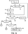
Returning to this step 44, it can notably include, in the case where several objects are prosecuted (K> 1), the resolution of cases of occlusion, or more generally cases of ambiguity between several objects for the attribution of Event. In step 43, the respective distances d (m _k , p) between the event ev (p, t) and the nearest points m _k of the models G _k of the different objects pursued have been calculated. If only one of these distances d (m _k , p) is less than a threshold d _th , for example d _th = 3 pixels, then the event is attributed to this object. In the opposite case, it is considered as an ambiguous event, attributable to several different objects.

This treatment is illustrated by the figure 14 . It starts at step 50 by index initialization k and j at 1 and 0, respectively. It is examined during the test 51 if the distance d (m _k , p) that has been minimized in step 43 is less than the threshold d _th and if so, the index j is incremented by one unit to step 52 and the jth entry of a table k (j) is taken equal to k in step 53. After step 53, or when d (m _k , p) ≥ d _th in the test 51 , it is examined during the test 54 if all the objects have been traversed (k = K). Yes k <K, the test 54 is followed by an incrementation of one unit of the index k in step 55 and then by a return to the next test 51. When k = K on the test 54, the integer j is evaluated. If j = 0, no object is considered to have its model close enough to the detected event ev (p, t), and the event is rejected (return to step 41 of the figure 11 ). If j = 1, the event ev (p, t) is assigned to the object k = k (1) (move to step 45 of the figure 11 ). If j> 1, it is necessary to proceed to a clearing of ambiguity 56 between the objects k (1), ..., k (j).

• Attribuer au plus proche : un nouvel événement ev(p, t) est attribué à l'objet k (parmi k(1), ..., k(j)) dont le modèle G_k est le plus proche, c'est-à-dire celui qui minimise d(m_k, p). En théorie, cette stratégie fonctionne correctement si le nouvel événement correspond parfaitement au modèle G_k et si les données ne contenaient pas de bruit et en l'absence d'ambiguïté due aux occlusions ;
• Rejeter tous : cette approche ignore simplement les événements ambigus, c'est-à-dire que les étapes 45-47 de la figure 11 ne sont pas exécutées pour l'événement ev(p, t). Cette approche paraît logique puisqu'a priori il n'est pas possible de prendre une décision claire. Néanmoins, la poursuite peut échouer dans la mesure où la dynamique de la forme risque d'être perdue ;
• Mettre à jour tous : tous les modèles G_k avoisinant un événement ambigu ev(p, t) sont mis à jour. En d'autres termes, les étapes 45-47 de la figure 11 sont exécutées pour chaque objet k tel que d(m_k, p) ≤ d_th ;
• Mise à jour pondérée : un événement ambigu ev(p, t) contribue à chaque modèle avoisinant G_k avec une pondération variant en sens contraire de la distance. En d'autres termes, les étapes 45-47 de la figure 11 sont exécutées pour chaque objet k tel que d(m_k, p) ≤ d_th avec un coefficient de pondération respectif α_k calculé comme une fonction décroissante de la distance d(m_k, p), par exemple inversement proportionnel à d(m_k, p)) et tel que ∑α_k = 1.

Consideration of spatial constraints in the removal of ambiguities 56 can take place according to several strategies:

• Assign to the nearest : a new event ev (p, t) is assigned to the object k (among k (1), ..., k (j)) whose model G _k is the closest, that is that is, the one that minimizes d (m _k , p). In theory, this strategy works correctly if the new event fits perfectly with the G _k model and if the data contained no noise and no ambiguity due to occlusions;
• Reject all: this approach simply ignores ambiguous events, that is, steps 45-47 of the figure 11 are not executed for the event ev (p, t). This approach seems logical since, in principle, it is not possible to make a clear decision. Nevertheless, the pursuit may fail to the extent that the dynamics of the form may be lost;
• Update all: All models G _k neighboring an ambiguous event ev (p, t) are updated. In other words, steps 45-47 of the figure 11 are executed for each object k such that d (m _k , p) ≤ d _th ;
• Weighted update : an ambiguous event ev (p, t) contributes to each model around G _k with a counter-to-distance weighting. In other words, steps 45-47 of the figure 11 are executed for each object k such that d (m _k , p) ≤ d _th with a respective weighting coefficient α _k calculated as a decreasing function of the distance d (m _k , p), for example inversely proportional to d (m _k , p)) and such that Σα _k = 1.

The very high temporal resolution of the event-based acquisition process provides additional information for the resolution of ambiguous situations. We can determine a current event rate r _k for each form continued G _k , which contains information about the object k and partly encodes the dynamics of this object.

We denote here t _{k, 0} , t _{k, 1} , ..., t _{k, N (k)} the temporal labels of the most recent events, to the number of N (k) +1, which have been attributed to an object k during a time window whose length Δt can be of the order of a few milliseconds to a few tens of milliseconds, with t _{k, 0} <t _{k, 1} <... <t _{k, N (k)} ( the event detected at t _{k, N (k)} is therefore the most recent for object k). These time labels make it possible to calculate for each object k a sliding average of the event rate r _k , defined by: $$r_k=\frac{\mathrm{NOT}\left(k\right)}{t_{k,\mathrm{NOT}\left(k\right)}-t_{k,0}}$$

This calculation of the current event rate r _k can take place as soon as an event has been assigned to the object k (step 44) following the detection of this event at time t _{k, N (k)} .

Then, when an next event ev (p, t) gives rise to an ambiguity between several pursued objects, step 44 can comprise the computation of a score C _k for each object k to which the ambiguous event ev (p, (t) is attributable, in the words $${\mathrm{VS}}_{\mathrm{k}}=\left(\mathrm{t}-{\mathrm{t}}_{\mathrm{k},\mathrm{NOT}\left(\mathrm{k}\right)}\right){\mathrm{r}}_{\mathrm{k}}$$

This score C _k makes it possible to evaluate the temporal coherence of the ambiguous event ev (p, t) with each object k. we can expect the duration t - t _{k, N (k) to} be close to the inverse of the current rate r _k if the event ev (p, t) belongs to the object k. Taking into account the time constraint in step 44 then consists, after calculating the score C _k according to (14), to choose among the different case objects to which the event ev (p, t) is attributable, that for which the score is closest to 1. Once this choice has been made, we can update the rate r _k for the chosen object and go to step 45 of the figure 11 .

This processing taking into account temporal constraints for the removal of ambiguities, and constituting a mode of execution of the step 56 of the figure 14 , is illustrated by the figure 15 . It begins at step 60 by initializing an index i to 1, the object index k being initialized to k (1) and the score C to (t - t _{k (1), N (k ( 1))} ) r _{k (1)} . A 61-65 loop is performed to evaluate the scores C _{k (i)} of the different objects to which the event ev (p, t) is attributable. In step 61, the index i is incremented by one. In step 62, the score C _{k (i)} of the object k (i) is calculated according to C '= (t - t _{k (i), N (k (i))} ) r _{k (i)} . If | C '- 1 | ≥ | C - 1 | (test 63), the loop output test 65 is executed to compare the index i with the number j of candidate objects. If | C '- 1 | <| C - 1 | in test 63, step 64 is executed to replace the index k by k (i) and update C = C 'before going to the loop output test 65. As long as i <j on test 65, the process returns to step 61 for the next iteration. When i = j, the assignment of the event to the object k has been completed and the algorithm proceeds to step 66 of updating the number N (k) and time tags t _{k, 0} , t _{k , 1} , ..., t _{k, N (k)} for the object k that has been selected. Then, the rate r _k is updated according to (12) in step 67 and the algorithm goes to step 45 of the figure 11 .

Another way of removing the ambiguity in step 56 is to combine spatial and temporal constraints by referring to the displacement planes Π _{k (1)} , ..., Π _{k (j)} of the different objects k (1). ), ..., k (j) attributable to the event ev (p, t).

avec : $$\mathrm{D}\left(\mathrm{i}\right)=\left|{\mathrm{eg}}_{\mathrm{k}\left(\mathrm{i}\right)}.{\mathrm{n}}_{\mathrm{k}\left(\mathrm{i}\right)}\right|$$

où « . » désigne le produit scalaire entre deux vecteurs dans l'espace à trois dimensions, n_k(i) est le vecteur donnant la direction de la normale au plan Π_k(i) et eg_k(i) est le vecteur allant du point e marquant l'événement détecté ev(p, t) dans l'espace à trois dimensions à l'un des points g_k(i) du plan Π_k(i).In particular, we can use for the assignment of the event ev (p, t) the object k which, among k (1), ..., k (j), minimizes the distance, measured in the space representation three-dimensional time between the event ev (p, t) and each plane Π _{k (1)} , ..., Π _{k (j)} . The event is then assigned to the object k such as: $$k=\underset{i=1.2,...,j}{\mathit{Arg}\min }D\left(i\right)$$

with: $$\mathrm{D}\left(\mathrm{i}\right)=\left|{\mathrm{eg}}_{\mathrm{k}\left(\mathrm{i}\right)}.{\mathrm{not}}_{\mathrm{k}\left(\mathrm{i}\right)}\right|$$

or " . Is the scalar product between two vectors in three-dimensional space, n _{k (i)} is the vector giving the direction of the normal to the plane Π _{k (i)} and eg _{k (i)} is the vector from point e marking the detected event ev (p, t) in the three-dimensional space at one of the points g _{k (i)} of the plane Π _{k (i)} .

This treatment combining spatial and temporal constraints for the removal of ambiguities, and constituting another mode of execution of the step 56 of the figure 14 , is illustrated by the figure 16 . It starts at step 70 by initializing an index i to 1, the object index k being initialized to k (1) and the distance D to | eg _{k (1)} . n _{k (1)} |. A 71-75 loop is performed to evaluate the distances D (i) for the different objects to which the event ev (p, t) is attributable. In step 71, the index i is incremented by one unit. In step 72, the distance D (i) for the object k (i) is calculated according to D = | eg _{k (i)} . n _{k (i)} |. If D ≥ ≥ D (test 73), the loop output test 75 is executed to compare the index i with the number j of candidate objects. If D '<D at test 73, step 74 is executed to replace index k by k (i) and update D = D' before switching to test 75. As long as i <j at test 75, the process returns to step 71 for the next iteration. When i = j, the assignment of the event to the object k has been completed and the algorithm goes to step 45 of the figure 11 .

When the asynchronous sensor 10 is in motion, events are also generated by the fixed background of the scene. The figure 17 shows the typical distance distribution between the events belonging to a continued object k and the estimated displacement plane Π _k for this object (curve 78), as well as the typical distance distribution between the events belonging to the fixed background and the displacement plane of the object (curve 79). This shows that the average displacement plane Π _k can provide a discriminating criterion for separating the events concerning an object pursued k from those concerning unexcused objects including the background. Events that are inconsistent with the object pursued or, equivalently, "too far" from the displacement plane Π _k are simply ignored.

One way of filtering the events coming from the backdrop is then to estimate the statistical distribution of the distances between the plane of displacement Π _k of the object pursued (estimated at step 47 of FIG. figure 11 ) and the points marking the detected events ev (p, t) that were assigned to this object in step 44 during a time window Δt. This statistical distribution corresponds to curve 78 of the figure 17 . It evaluates the average distance d _k between the displacement plane Π _k and the events attributed to the object as well as the standard deviation σ _k of the distribution. From these parameters, an interval I _k of admissible values of the distance is determined. When it is necessary to decide whether a new detected event ev (p, t) must be assigned to the object pursued, the distance D = | eg _k .n _k | between the point marking the event ev (p, t) in the three-dimensional space and the plane Π _k . If this distance D falls outside the interval I _k , the event is not attributed to the object k. On the other hand, the event is assigned to the object k, or subjected to other filtering, in particular to take into account any occlusions as discussed above with reference to the Figures 14-16 .

For example, the interval I _k is centered on the average distance value d _k , and its width is a multiple of the standard deviation σ _k .

To take into account the possible movement of the substance, step 44 of the figure 11 can include the illustrated treatment the figure 18 (In the particular case where a single object k is pursued, this case can easily be generalized to that where K> 1). After detecting the event ev (p, t) in step 42, the distance D = | eg _k .n _k | is calculated in step 80 then the test 81 is executed to determine if this distance D falls in the interval I _k . If D is outside of I _k , the process returns to step 41 of the figure 11 . If D falls into I _k , the event ev (p, t) is assigned to the object k rather than the movement of the background. The distance distribution relative to the displacement plane Π _k of the object k (curve 78) is then updated with the distance D in step 82, then the interval I _k is recalculated at step 83. process then passes step 45 of the figure 11 .

The treatments described with reference to Figures 14-18 have been presented in the context of an embodiment of the invention following the figure 11 . However, it will be observed that these treatments, serving to take into account the possible occlusions between multiple objects pursued as well as the possible movement of the back of the stage, can also be used with other embodiments of the process of pursuit of form, in particular when an SVD type technique is used as described with reference to the figure 8 which does not represent an embodiment of the invention.

Numerical experiments have been conducted to demonstrate the performance of the method set forth above. These experiments are reported in the following examples.

Example 1

The experiment was carried out in the case of a star drawn on a rotating disk, as indicated above with reference to Figures 6A and 7 , looking for a rigid spatial transformation F _t , that is to say composed of a translation and a rotation in the plane of the images.

The disc was spinning at a speed of 670 revolutions per minute. The pattern H giving the shape of the model G was manually generated by selecting 6 points per side of the star from a snapshot. A 6-pixel distance threshold was used to eliminate the impact of noise and reduce computational load. As illustrated by figure 7 , the algorithm succeeds in continuing the rotating form efficiently despite the high rotation speed.

• algorithme ICP traitant les images d'une caméra classique dont le signal de sortie se compose de trames (courbe 85 sur la figure 19). Pour que la comparaison soit juste, seuls les emplacements de pixels restant après différenciation des trames sont considérés par l'algorithme ICP ;
• méthode de poursuite de forme utilisant le capteur asynchrone basé sur événement 10 avec estimation en forme analytique reposant sur une approche SVD, de la manière indiquée en référence à la figure 8 (courbe 86), en considérant des événements collectés sur une période de temps de 50 µs ;
• méthode de poursuite de forme utilisant le capteur asynchrone basé sur événement 10 avec estimation du modèle mis à jour en fonction de l'association courante entre un pixel p de la matrice d'où provient un événement ev(p, t) et un point m du modèle, indépendamment des associations effectuées avant la détection de cet événement, de la manière indiquée en référence à la figure 11 (courbe 87).

The figure 19 allows to compare the accuracy of the continuation of the star shape obtained with three methods of pursuit:

• ICP algorithm processing the images of a conventional camera whose output signal consists of frames (curve 85 on the figure 19 ). For the comparison to be fair, only the remaining pixel locations after frame differentiation are considered by the ICP algorithm;
• shape-tracking method using the event-based asynchronous sensor 10 with analytically-based estimation based on an SVD approach, as indicated with reference to the figure 8 (curve 86), considering events collected over a period of time of 50 μs;
• shape-tracking method using the event-based asynchronous sensor 10 with estimation of the updated model according to the current association between a pixel p of the matrix from which an event ev (p, t) comes from and a point m of the model, irrespective of the associations made prior to the detection of that event, as indicated with reference to the figure 11 (curve 87).

To evaluate the accuracy of shape tracking, the average distance between the model set and the locations of active events is calculated every 200 μs. The average errors are respectively 2.43, 1.83 and 0.86 pixels for the curves 85, 86 and 87, with respective standard deviations of 0.11, 0.19 and 0.20 pixels. Taking into account the asynchronous signal of the sensor allows a significant improvement of the shape tracking method, especially in the case of the figure 11 .

The superior temporal accuracy leads to a more accurate tracking. The error curve presents oscillations (box of the figure 19 ) due to the repetitive rotation of the stimulus. The tracking error demonstrates the good reproducibility and reliability properties of the algorithm. The residual error is due to the geometry of the square pixel matrix combined with the limited spatial resolution of the sensor, which does not provide an isotropic response to the angular position of the shape.

The number of points selected for the G model has an influence on the cost and accuracy of the calculations.

In the case of a realization according to the figure 11 an equivalent frame rate can be defined as the inverse of the computation time required to process an event.

In the example, the tracking program was run on a computer equipped with a central processing unit (CPU) type "Intel Core i5" clocked at 2.8 GHz and occupied 25% of the capacity of this CPU. In this configuration, it appeared that a size of 90 points in the model can provide a detection frequency corresponding to an equivalent frame rate of 200 kHz. Up to about 2000 points in the model, it can be updated with an equivalent frame rate of at least 11 kHz. Experience has shown that for a model with 60 to 70 points, the algorithm is able to continue in real time a shape moving at a speed of up to 1250 rpm.

In general, there is interest in including the corners of the object's outline in the model. Along a straight edge of the shape of the object, however, it is possible to reduce the number of points without negatively influencing the final accuracy of the pursuit.

When the number of points increases, the tracking error does not tend to zero, but to a value of about 0.84 pixels, related to the spatial resolution limit of the asynchronous sensor. Logically, the more points the model contains, the better the accuracy of the chase, but with a higher computational cost. A size of 60 to 100 points for the model is a good compromise to obtain a reasonable accuracy (around 0.90 pixels) while preserving a high tracking frequency (around 200 kHz).

Example 2

The experiment was carried out in the case of several forms (an H-shape, a car shape and a star shape) taking into account an affine spatial transformation calculated using expressions (6), (7) , (11) and (12) in an embodiment according to figure 11 . During this experiment, the shapes of the objects were deformed and resized in the manner shown on the figure 20 (ad for the H shape, eh for the car shape, it for the star shape).

The figure 21 shows the scaling factors s _x , s _y in relation to the original size of the shape, during the continuation of the car shape (curves 90 and 91, respectively). Scale ratios are different along both axes because perspective changes occurred more often along the vertical axis than along the horizontal axis during the experiment. The tracking error (plot 92) showed an average value of 0.64 pixels and a standard deviation of 0.48 pixels.

The process described above with reference to figure 11 therefore provides good performance when looking for an affine transformation.

Example 3

In this experiment, car traffic data was acquired with the asynchronous sensor. As shown in figure 22 at four successive instants, several vehicles were moving simultaneously on several queues. Column (a) of the figure 22 shows the events generated by the asynchronous sensor and accumulated for a few microseconds, while column (b) shows corresponding gray-scale images. We can see that the chosen scene presented critical moments with strong occlusions due to static objects (trees, lampposts, ...) and to moving objects (vehicles) which constituted a significant challenge for the robust pursuit.

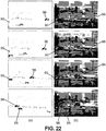
Two forms 95, 96 respectively corresponding to a car and a van were continued by the method illustrated by the figure 11 , looking for affine transformations F _t . The convergence steps η ₁ , η ₂ and η ₃ of the expressions (6), (7), (11) and (12) have respectively been fixed at 0.1, at 0.002 and at 10 ^-5 . The G ₁ model for the car had 67 points, while the G ₂ model for the car van had 102 points. These models were generated by manually pointing pixels of an acquired image.

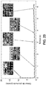
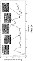
The figure 23 shows the tracking errors found with a process in accordance with the figure 11 and an asynchronous event-based sensor, while the figure 24 shows the same errors found with a conventional method using images from a frame-based camera. For the comparison to be relevant, the conventional frame-based ICP technique was applied to reconstructed gray-scale images at a frequency of 100 frames per second. Each image was pretreated to obtain moving edges by calculating a difference between the successive frames and applying a thresholding operation. The time precision of the event-based method was of the order of 1 μs.

The average tracking error was 0.86 pixels with a standard deviation of 0.19 pixels for the event-based method according to the figure 11 ( figure 23 ), while the conventional frame-based method resulted in an average tracking error of 5.70 pixels with a standard deviation of 2.11 pixels ( figure 24 ). Thumbnails (a1) - (a5) on the figure 23 and (b1) - (b5) on the figure 24 show situations where the "van" object encounters occlusions, giving rise to maxima of tracking error.

It is remarkable that the superior temporal accuracy provided by the method according to the invention is accompanied by better tracking stability than the conventional frame-based method. In the conventional method, the (expensive) solution of increasing the acquisition frequency is not always sufficient to correctly treat occlusion situations. Conversely, the dynamic content of the event-based signal produced by the asynchronous sensor provides more stable input data for the algorithm. Static obstacles do not generate events and therefore have virtually no impact on the prosecution process.

Example 4

Several ambiguity strategies have been tested for tracking multiple objects that may have occlusions.

The shapes of a "car" object and a "van" object moving in the same direction but with different speeds were continued simultaneously in a real scene including car traffic. For a time, the shapes of the van and the car are superimposed in the field of view of the sensor 10, until the van passes the car. Objects other than the van and the car are treated as background noise.

• les distances observées entre un événement provenant de l'objet « camionnette » et le centre de gravité de l'objet « camionnette » (courbe 100) ;
• les distances observées entre un événement provenant de l'objet « voiture » et le centre de gravité de l'objet « voiture » (courbe 101) ;
• les distances observées entre un événement provenant de l'objet « camionnette » et le centre de gravité de l'objet « voiture » (courbe 102) ; et
• les distances observées entre un événement provenant de l'objet « camionnette » et le centre de gravité de l'objet « voiture » (courbe 103).

The figure 25 shows:

• the distances observed between an event coming from the "van" object and the center of gravity of the "van" object (curve 100);
• the distances observed between an event coming from the "car" object and the center of gravity of the "car" object (curve 101);
• the distances observed between an event originating from the "van" object and the center of gravity of the "car" object (curve 102); and
• the distances observed between an event coming from the "van" object and the center of gravity of the "car" object (curve 103).

Ambiguities occur when these curves pass through similar values, meaning that the shapes of the two vehicles overlap in the field of view (between about 2.2 and 2.9 s). In this case, the use of spatial information may be insufficient unless the size of the common region is very small.

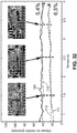
The figure 26 shows the average event rates r _k of the "van" object (curve 105) and the "car" object (curve 106). In this experiment, we see that the two curves are disjoint, so that the shapes of the two vehicles remain separable throughout the sequence with reference to event rates of the order of 3000 events per second for the car and the order of 5000 events per second for the van. However, this property of separability is not necessarily guaranteed for any sequence.

In the general case, it is typically preferable to combine the time constraint with additional constraints, such as spatial constraints.

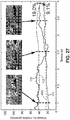
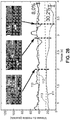
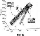
The Figures 27-32 show the speeds of the models of the "van" object (curve 110) and the "car" object (curve 111) estimated during the implementation of a method according to the figure 11 , comparing them to the actual speeds (dotted curves 112 and 113, respectively) determined manually by identifying the corresponding points on successive images. The average speeds were respectively 42.0 pixels / 0 for the van is 24.3 pixels / s for the car. The six figures correspond to six different strategies for the removal of ambiguity: "Attribute to the nearest" ( figure 27 ); "Reject all" ( figure 28 ); "Update all" ( figure 29 ); "Weighted update" ( figure 30 ); "Temporal constraint based on the rate r _k " ( figure 31 ); and "Combination of spatial and temporal constraints using the plane of displacement Π _k " ( figure 32 ). The vignettes included in the Figures 27-32 present the most interesting moments to study the differences between the methods. The beginning of each curve is the same as long as no occlusion has occurred. The percentages indicated in the straight portions of the graphs correspond to the average relative difference between the curves 110 and 112 on the one hand and between the curves 111 and 113 on the other hand.

We see on the figure 27 that the "Assign to the nearest" strategy provides rather mediocre results since the model of the van and lost due to its occlusion by the model of the car. The "Reject All" strategy ( figure 28 ) is not more satisfactory since, this time, it is the model of the car that is lost after the occlusion.

The "Update All" strategy ( figure 29 ) seems preferable since the shapes of the 2 vehicles continue without loss. At the end of the sequence, the events generated by the van attract the model of the car, so that the resulting trajectory for the car deviates slightly towards that of the van and that the estimated speed of the van decreases when that of the car increases (see (c3) on the figure 29 ).

The "Weighted Update" strategy divides the dynamics introduced by ambiguous events between different objects with distance-dependent weights. The figure 30 shows that the van and the car are pursued without loss and that the speed curves correspond better to actual speeds. There are still differences at the end of the sequence, for the same reason as in the "Update all" strategy , but with a smaller amplitude of these errors. This " Weighted Update " strategy is preferred among those based on spatial constraints when multiple objects intersect or collide.

The strategy "Temporal constraint based on cadence r _k " ( figure 31 ) works well in this experiment. However, its reliability is not assured when the target objects have similar event rates.

The strategy "Combination of spatial and temporal constraints using the displacement plane Π _k " was used with a period Δt of 3 s for the estimation of the displacement planes Π ₁ of the object "pickup truck" and Π ₂ of the object "car" ( figure 33 ). As shown in figure 32 , this strategy is the one that gives rise to the smallest error in the pursuit of both vehicles. This is explained by the fact that the local spatio-temporal plans Π ₁ , Π ₂ strongly constrain the neighborhood by eliminating bad attributions and by providing a better robustness to noise. It is interesting to note that the errors are spread more evenly between the van and the car thanks to the more reliable allocation process.

Example 5

Two asynchronous signal sequences generated by a moving sensor were tested by applying the method of eliminating the events generated by the background which has been described with reference to the figure 16 .

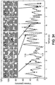
In the first sequence, a star shape was moved in an indoor environment while the asynchronous sensor was held by hand and stirred simultaneously. The figure 34 shows several snapshots of the scene (a1) - (a5).

To evaluate the results, the speed of the star calculated by the process according to the figure 11 (combining the movement of the star and that of the sensor) is shown by the curve 116 on the figure 34 , and compared to the actual speed manually pointed and indicated by the dotted line curve 117. The average error between the estimated data and the actual data is estimated at 6%. Although the scene has many edges in the background, the chase process remains robust.

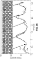
The second sequence comes from an outdoor scene with new car traffic. A form of car is continued using an asynchronous vision sensor 10 moved manually.

The figure 35 shows the results of the estimates of the speed of the car (curve 118) and compares them with actual actual speeds (curve 119). Despite situations that are difficult to treat (for example, when sidewalks or crosswalks are close to the car or superimposed), the good spatio-temporal properties of the algorithm provide acceptable results. The average estimation error on speed is 15%. The quality of the pursuit deteriorates from about 3.5 seconds (b5 on the figure 35 ), when the car begins to undergo significant perspective changes.

Overall, the event-based tracking as discussed above is robust even when the sensor and the objects being tracked are moving.

The embodiments described above are illustrations of the present invention. Various modifications can be made without departing from the scope of the invention which emerges from the appended claims.

Claims (18)

1. A method of tracking a shape in a scene, comprising:

   receiving asynchronous information from a light sensor (10) having a matrix of pixels arranged opposite the scene, wherein the asynchronous information comprises, for each pixel of the matrix, successive events originating asynchronously from said pixel; and

   updating a model (G) comprising a set of points and representing a tracked shape of an object, after detecting events attributed to said object in the asynchronous information, wherein the updating comprises, following detection of an event (ev(p, t)):

   associating with the detected event a point (m) of the model having a minimum distance with respect to the pixel (p) of the matrix from which the detected event originates; and

   determining the updated model according to the pixel (p) of the matrix from which the detected event originates and the associated point (m), and independently of the associations performed before the detection of said event (ev(p, t)).
2. The method of claim 1, wherein when no point of the model (G) is located at a distance less than a threshold (d_max, d_th) with respect to the pixel (p) from which a detected event (ev(p, t)) originates, the model is not updated following the detection of said event which is not attributed to the object.
3. The method of any one of the preceding claims, further comprising:

   estimating a plane of displacement of the object, wherein the plane of displacement (Π_k) is estimated in a space with three dimensions, namely two spatial dimensions corresponding to two directions of the matrix of pixels and one time dimension, by minimizing a distance criterion in relation to a set of points that mark detected events which were attributed to the object during a time window ending at a current instant; and

   following detection of an event (ev(p, t)), taking into account the estimated plane of displacement of the object in order to decide whether or not to attribute said event to the object.
4. The method of claim 3, wherein a plurality of objects have respective shapes tracked in the scene, wherein each one of the plurality of objects has a respective model (G_k) updated after detection of events attributed thereto and an estimated plane of displacement (Π_k), wherein the method further comprises, following detection of an event (ev(p, t)) attributable to at least two of the objects:

   calculating respective distances, in the three-dimensional space, between a point marking said detected event and the planes of displacement respectively estimated for said objects; and

   attributing said detected event to the object for which the calculated distance is minimal.
5. The method of claim 3 or claim 4, further comprising:

   estimating a statistical distribution of distances between the plane of displacement (Π_k) of the object and points marking detected events which were attributed to the object; and

   following detection of an event (ev(p, t)), taking into account the estimated plane of displacement of the object and the estimated statistical distribution in order to decide whether or not to attribute said event to the object.
6. The method of claim 5, further comprising:

   determining an interval (I_k) of admissible distance values based on the estimated statistical distribution; and

   not attributing a detected event to the object if the point marking said detected event in the three-dimensional space has, in relation to the estimated plane of displacement, a distance falling outside the interval of the admissible distance values.
7. The method of any one of the preceding claims, wherein a plurality of objects have respective shapes tracked in the scene, wherein each of the objects has a respective model (G_k) updated after detection of events attributed thereto, wherein the method further comprises, following detection of an event (ev(p, t)):
   if only one of the objects satisfies a condition of having in its model a point that has a distance less than a threshold (d_th) with respect to the pixel (p) of the matrix from which the detected event originates, attributing the detected event to said one of the objects.
8. The method of any one of the preceding claims, wherein a plurality of objects have respective shapes tracked in the scene, wherein each one of the objects has a respective model (G_k) updated after detection of events attributed thereto, wherein the method further comprises, following detection of an event (ev(p, t)) attributable to at least two of the objects:

   for each object to which the detected event is attributable, associating with the detected event a point (m) of the model (G_t) of said object by minimizing a respective distance criterion with respect to the pixel (p) of the matrix from which the detected event originates; and

   attributing the detected event to the object for which the minimized criterion of distance is lowest.
9. The method of any one of claims 1 to 7, wherein a plurality of objects have respective shapes tracked in the scene, wherein each one of the plurality of objects has a respective model (G_k) updated after detection of events attributed thereto, and wherein, following detection of an event (ev(p, t)) attributable to at least two of the objects, the detected event is not assigned to any of said at least two of the objects.
10. The method of any one of claims 1 to 7, wherein a plurality of objects have respective shapes tracked in the scene, wherein each one of the plurality of objects has a respective model (G_k) updated after detection of events attributed to it, and wherein, following detection of an event (ev(p, t)) attributable to at least two of the objects, the detected event is assigned to each one of the objects to which the detected event is attributable.
11. The method of claim 10, wherein updating the models (G_k) of objects to which the detected event is attributed is carried out with weightings that depend on the distance criteria respectively minimized for said objects.
12. The method of any one of claims 1 to 7, wherein a plurality of objects have respective shapes tracked in the scene, wherein each one of the plurality of objects has a respective model (G_k) updated after detection of events attributed thereto, the method further comprising:

    for each object, estimating a rate of events attributed to said object and memorizing an instant at which the last event attributed to said object was detected; and

    following detection of an event (ev(p, t)) attributable to at least two of the objects, attributing the detected event to the one of the objects for which the product of the estimated rate of events by the time interval between the memorized instant and the instant of detection of said event is closest to 1.
13. The method of any one of the preceding claims, wherein determining the updated model comprises estimating (45) a spatial transformation (F_t) defined by a set of parameters, and applying (46) the estimated spatial transformation to the model (G_k), and wherein estimating the spatial transformation comprises calculating said parameters as a function of a gradient of a distance, in the plane of the matrix of pixels, between the pixel (p) of the matrix from which the detected event originates and a point obtained by applying the spatial transformation to the point (m) of the model associated with the detected event.
14. The method of claim 13, wherein the spatial transformation (F_t) includes a translation and a rotation in the plane of the matrix of pixels, wherein the translation has a vector ΔT taken equal to - η₁.∇_Tf(Δθ₀, ΔT₀) and the rotation has an angle Δθ taken equal to - η₂.∇_θf(Δθ₀, ΔT₀), where η₁ and η₂ are predefined positive convergence steps and Δθ₀ and ΔT₀ are particular values of the angle of rotation and of the translation vector.
15. The method of claim 14, wherein said particular values of the angle of rotation and of the translation vector are respectively ${\mathrm{\Delta \theta }}_0=\widehat{\mathit{mcp}}$

    

    and ΔT₀ = cp - R_Δθ0 [cm], where p designates the pixel of the matrix from which the detected event originates, m designates the point of the model associated with the detected event, c designates the center of the rotation, cp designates a vector pointing from c to p, cm designates a vector pointing from c to m, and R_Δθ0 [.] is the rotation of center c and of angle Δθ₀.
16. The method of claim 14 or claim 15, wherein the spatial transformation (F_t) is an affine transformation further including application of respective scaling factors according to two axes included in the matrix of pixels.
17. The method of claim 16, wherein the scaling factors s_x, s_y according to the two axes x, y are respectively calculated according to s_x = 1 + η₃.(|p_x| - |m_x|) and s_y = 1 + η₃.(|p_y| - |m_y|), where η₃ is a predefined positive convergence step, p_x and p_y are respective coordinates, according to the axes x and y, of the pixel (p) of the matrix from which the detected event originates, and m_x and m_y are respective coordinates, according to the axes x and y, of the point (m) of the model associated with the detected event.
18. A device for tracking a shape in a scene, comprising a computer (20) configured to execute a method as claimed in any one of the preceding claims using asynchronous information received from a light sensor (10).

Images