WO2024257533A1 - 被覆導線および多芯ケーブル - Google Patents
被覆導線および多芯ケーブル Download PDFInfo
- Publication number
- WO2024257533A1 WO2024257533A1 PCT/JP2024/017783 JP2024017783W WO2024257533A1 WO 2024257533 A1 WO2024257533 A1 WO 2024257533A1 JP 2024017783 W JP2024017783 W JP 2024017783W WO 2024257533 A1 WO2024257533 A1 WO 2024257533A1
- Authority
- WO
- WIPO (PCT)
- Prior art keywords
- conductor
- wire
- twist pitch
- cross
- strands
- Prior art date
- Legal status (The legal status is an assumption and is not a legal conclusion. Google has not performed a legal analysis and makes no representation as to the accuracy of the status listed.)
- Ceased
Links
Images











Classifications
-
- B—PERFORMING OPERATIONS; TRANSPORTING
- B21—MECHANICAL METAL-WORKING WITHOUT ESSENTIALLY REMOVING MATERIAL; PUNCHING METAL
- B21F—WORKING OR PROCESSING OF METAL WIRE
- B21F7/00—Twisting wire; Twisting wire together
-
- G—PHYSICS
- G06—COMPUTING OR CALCULATING; COUNTING
- G06T—IMAGE DATA PROCESSING OR GENERATION, IN GENERAL
- G06T5/00—Image enhancement or restoration
- G06T5/60—Image enhancement or restoration using machine learning, e.g. neural networks
-
- G—PHYSICS
- G06—COMPUTING OR CALCULATING; COUNTING
- G06T—IMAGE DATA PROCESSING OR GENERATION, IN GENERAL
- G06T7/00—Image analysis
-
- H—ELECTRICITY
- H01—ELECTRIC ELEMENTS
- H01B—CABLES; CONDUCTORS; INSULATORS; SELECTION OF MATERIALS FOR THEIR CONDUCTIVE, INSULATING OR DIELECTRIC PROPERTIES
- H01B5/00—Non-insulated conductors or conductive bodies characterised by their form
- H01B5/08—Several wires or the like stranded in the form of a rope
-
- H—ELECTRICITY
- H01—ELECTRIC ELEMENTS
- H01B—CABLES; CONDUCTORS; INSULATORS; SELECTION OF MATERIALS FOR THEIR CONDUCTIVE, INSULATING OR DIELECTRIC PROPERTIES
- H01B7/00—Insulated conductors or cables characterised by their form
- H01B7/04—Flexible cables, conductors, or cords, e.g. trailing cables
Definitions
- multi-core cables that include a conductor made of multiple strands twisted together and a coating that covers the conductor (see, for example, International Publication No. 2017/056278).
- Conductors made of multiple strands twisted together are manufactured using, for example, a bobbin fixed type manufacturing device or a bobbin rotating type manufacturing device (see, for example, Japanese Patent Application Laid-Open Nos. 2006-328603 and 4-075733).
- the coated conductor of the present disclosure comprises a conductor portion and a coating portion.
- the coating portion coats the conductor portion.
- the conductor portion is formed by twisting together a number of strands.
- the conductor portion includes a conductor.
- the conductor is adjacent to the coating portion.
- the direction in which the conductor portion extends is the Z direction.
- the conductor has a half-width of 15.5 mm or less. The half-width is calculated from a histogram of the twist pitch of the conductor in the Z direction.
- FIG. 1 is a cross-sectional view of a multi-core cable according to the present embodiment.
- FIG. 2 is a cross-sectional view of a covered conductor in a multi-core cable according to the present embodiment.
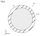
- FIG. 3 is a cross-sectional view of a covered conductor in a multi-core cable according to the present embodiment.
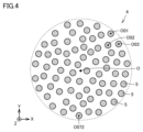
- FIG. 4 is a cross-sectional view of a conductor portion in a multi-core cable according to the present embodiment.
- FIG. 5 is a schematic cross-sectional view of a conductor portion for explaining a method of calculating the twist pitch of the wires.
- FIG. 6 is a schematic distribution diagram illustrating a histogram of the twist pitch.
- FIG. 7A is a schematic diagram showing an apparatus for manufacturing a conductor in which a plurality of strands of a multi-core cable are twisted together according to the present embodiment.
- FIG. 7B is a schematic diagram showing a multi-core cable manufacturing apparatus according to the present embodiment.
- FIG. 8 is a diagram showing the configuration of a quality evaluation system 40 for a multi-core cable.
- FIG. 9 is a diagram showing the configuration of learning device 60.
- FIG. 10 is a diagram illustrating an example of a convolutional neural network according to the present embodiment.
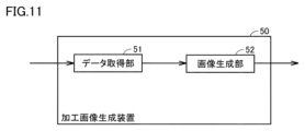
- FIG. 11 is a diagram showing the configuration of the processed image generating device 50.
- FIG. 12A is a diagram showing a tomographic image input to the neural network.
- FIG. 12A is a diagram showing a tomographic image input to the neural network.
- FIG. 12B is an enlarged view of the rectangular area in FIG. 12A.
- FIG. 13B is an enlarged view of the rectangular area in FIG. 13A.
- FIG. 14B is an enlarged view of the rectangular area in FIG. 14A.
- FIG. 15B is an enlarged view of the rectangular area in FIG. 15A.
- FIG. 15B is an enlarged view of the rectangular area in FIG
- FIG. 16B is an enlarged view of the rectangular area in FIG. 16A.
- FIG. 17B is an enlarged view of the rectangular area in FIG. 17A.
- FIG. 18B is an enlarged view of the rectangular area in FIG. 18A.
- FIG. 19B is an enlarged view of the rectangular area in FIG. 19A.
- FIG. 20B is an enlarged view of the rectangular area in FIG. 20A.
- FIG. 21B is an enlarged view of the rectangular area in FIG. 21A.
- FIG. 22B is an enlarged view of the rectangular area in FIG. 22A.
- FIG. 23B is an enlarged view of the rectangular area in FIG. 23A.
- FIG. 24B is an enlarged view of the rectangular area in FIG. 24A.
- FIG. 25B is an enlarged view of the rectangular area in FIG. 25A.
- FIG. 26B is an enlarged view of the rectangular area in FIG. 26A.
- FIG. 27B is an enlarged view of the rectangular area in FIG. 27A.
- FIG. 28B is an enlarged view of the rectangular area in FIG. 28A.
- FIG. 29 is a diagram illustrating appropriate and optimal values for the number of filters and filter sizes for the convolutional neural network of FIG.
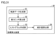
- FIG. 30 shows the configuration of the center position detection device 70. As shown in FIG. FIG. 31 shows the configuration of the index calculation device 80.
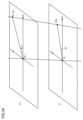
- FIG. 32 is a diagram showing an example of connection at the center position of the cross section of the wire.
- FIG. 33 is a diagram showing an example of trajectory data of each wire.
- FIG. 34 is a diagram for explaining the first twist pitch.
- FIG. 35 is a diagram for explaining the second twist pitch.
- FIG. 36 is a diagram for explaining the third twist pitch.
- FIG. 37 is a diagram for explaining the first twist pitch.
- FIG. 38 is a flow chart showing the operation procedure during learning.
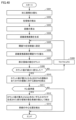
- FIG. 39 is a flow chart showing a procedure for evaluating the quality of a multi-core cable.
- FIG. 40 is a flow chart showing the procedure for detecting the center position in step S202.
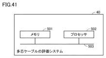
- FIG. 41 is a diagram showing a configuration in which the functions of the quality evaluation system 40 for a multi-core cable are realized by using software.
- FIG. 42 is a schematic diagram showing an apparatus for manufacturing a conductor in which a plurality of wires of the multi-core cables according to Samples 9 and 10 are twisted together.
- a multi-core cable connected to a sensor used in an anti-lock brake system (ABS) or an electric parking brake (EPB) can be bent in a complex manner due to driving of an actuator, etc. Therefore, there is a demand for improving the bending resistance of the multi-core cable.
- the present disclosure has been made to solve the above-mentioned problems. More specifically, it is an object of the present invention to provide a covered conductor wire and a multi-core cable having improved bending resistance. [Effects of this disclosure] According to the present disclosure, it is possible to obtain a covered conductor and a multi-core cable having improved bending resistance.
- An image generating method includes the steps of acquiring a tomographic image of a cross section perpendicular to the longitudinal direction of an object including multiple rod-shaped materials or multiple rod-shaped hollows, and generating an image from the acquired tomographic image in which the pixel at the center of the cross section of the material or hollow in the acquired tomographic image is bright and the pixels gradually become darker in the radial direction of the cross section of the material or hollow, using a trained model that generates an image from the acquired tomographic image in which the pixel at the center of the cross section of the material or hollow in the acquired tomographic image is bright and the pixels gradually become darker in the radial direction of the cross section of the material or hollow. This makes it possible to generate an image that is easily divided into a single material or hollow when multiple materials or hollows are in contact.
- the trained model is composed of a convolutional neural network with three convolutional layers.
- a trained model can be generated by a convolutional neural network with three convolutional layers that has high learning ability and is efficient.
- the size of one side of the filter in the first convolutional layer is the number of pixels that corresponds to a size that is 0.88 times or more and 2.64 times or less the diameter of the cross section of the material or hollow space. This allows the processing capacity of the first convolutional layer to be appropriately set.
- the size of one side of the filter in the third convolutional layer is the number of pixels that corresponds to a size that is 0.59 to 1.47 times the diameter of the cross section of the material or hollow space. This allows the processing capacity of the third convolutional layer to be appropriately set.
- a quality evaluation method for a multi-core cable includes the steps of generating a tomographic image and generating an image as described in any one of (1) to (4) above, and the step of acquiring the tomographic image includes the step of acquiring a tomographic image of a cross section perpendicular to the longitudinal direction of a multi-core cable including a plurality of strands, and the step of generating an image includes the step of generating, for each of the tomographic images of the plurality of cross sections of the multi-core cable, an image in which a pixel at the center of the cross section of the strand in the tomographic image is bright and the pixels become gradually darker in the radial direction of the cross section of the strand.
- the quality evaluation method for a multi-core cable further includes the steps of detecting the center position of the cross section of the strand from the generated image, determining the trajectory of the strand by connecting the center positions of the cross sections of the strand in the plurality of cross sections, and calculating an index representing the twist pitch of the strand based on the trajectory of the strand, or calculating an index representing the twist pitch of an assembly in which a plurality of strands are twisted together based on the trajectories of the strands.
- the step of detecting the center position includes a step of binarizing the obtained image. This makes it possible to properly separate an image that is likely to be separated into a single strand into a single strand.
- the method for evaluating the quality of a multi-core cable according to (5) above further includes a step of calculating statistics of an index representing the twist pitch.
- the statistics representing the twist pitch can be used to evaluate the quality of the multi-core cable.
- the statistic of the index representing the twist pitch is the half-width of the frequency calculated from a histogram of the index representing the twist pitch.
- the quality of the multi-core cable can be evaluated according to whether the twist pitch has a large variation as the statistic of the index.
- a coated conductor according to one embodiment of the present disclosure includes a conductor portion and a coating portion.
- the coating portion coats the conductor portion.
- the conductor portion is formed by twisting together a plurality of strands.
- the conductor portion includes a conductor.
- the conductor is adjacent to the coating portion.
- the direction in which the conductor portion extends is the Z direction.
- the conductor has a half-width of 15.5 mm or less. The half-width is calculated from a histogram of the twist pitch of the conductor in the Z direction.
- the twist pitch may be calculated based on the displacement of the relative position of the wires between the two cross sections in a relative coordinate system.
- the relative coordinate system may have the center of gravity of the conductor in the cross section as its origin.
- the distance between the two cross sections may be 1 mm.
- the histogram may be created from the amount of displacement of the relative positions of each of the multiple strands.
- the histogram may be created for a portion of the conductor that is 50 mm long in the Z direction.
- the conductor may include a first outer conductor and a second outer conductor.
- the histogram may be created from the twist pitch of each of the first outer conductor and the second outer conductor.
- the conductor portion may include an inner conductor.
- the inner conductor may be disposed away from the coating portion.
- a multi-core cable according to one embodiment of the present disclosure may include a coated conductor wire according to any one of (9) to (15) above.
- FIG. 1 is a cross-sectional view of a multi-core cable 1 according to the present embodiment.
- the multi-core cable 1 according to the embodiment of the present disclosure is, for example, a sensor used in an ABS of a vehicle or a multi-core cable 1 connected to an electric parking brake, and mainly includes a plurality of covered conductor wires 2 and a sheath layer 30.
- the covered conductor wires 2 are surrounded by the sheath layer 30.
- the plurality of covered conductor wires 2 are composed of two covered conductor wires 2a and two covered conductor wires 2b.
- the number of covered conductor wires 2 is not particularly limited.
- the multi-core cable 1 may include at least one of the covered conductor wires 2a and the covered conductor wire 2b.
- the number of covered conductor wires 2a may be 3 or more, or may be 1.
- the number of covered conductor wires 2b may be 3 or more, or may be 1.
- the number of covered conductor wires 2b may be 0.
- the direction in which the multi-core cable 1 extends is the Z direction (the Z direction shown in Figure 1).
- the directions perpendicular to the Z direction are the X direction and the Y direction.
- the X direction is perpendicular to the Y direction.
- the cross section shown in Figure 1 is a plane perpendicular to the Z direction.
- the sheath layer 30 may have a two-layer structure. Specifically, the sheath layer 30 includes an outer sheath layer 31 and an inner sheath layer 32. The two coated conductor wires 2a and the two coated conductor wires 2b are surrounded by the outer sheath layer 31. The inner sheath layer 32 is disposed inside the outer sheath layer 31. Specifically, the inner sheath layer 32 covers the outer circumference of each of the two coated conductor wires 2a and the two coated conductor wires 2a so as to fill the space between the outer sheath layer 31 and the coated conductor wires 2.
- the main component of the inner sheath layer 32 may be a flexible synthetic resin.
- the material constituting the inner sheath layer 32 may be, for example, a polyolefin such as polyethylene or EVA (Ethylene-Vinyl Acetate), a polyurethane elastomer, or a polyester elastomer.
- the main component of the outer sheath layer 31 may be a synthetic resin that has excellent flame retardancy and abrasion resistance.
- the material constituting the outer sheath layer 31 may be, for example, polyurethane.
- the shape of the outer sheath layer 31 is annular.
- the inner sheath layer 32 is connected to the inner peripheral surface of the outer sheath layer 31.
- the shape of the outer periphery 32a of the inner sheath layer 32 is circular.
- the minimum distance from the outer periphery 32a of the inner sheath layer 32 to the coated conductor wire 2 is preferably 0.3 mm, more preferably 0.4 mm.
- the maximum distance from the outer periphery 32a of the inner sheath layer 32 to the coated conductor wire 2 is preferably 0.9 mm, more preferably 0.8 mm.
- the minimum outer diameter of the inner sheath layer 32 is preferably 6.0 mm, more preferably 7.3 mm.
- the maximum outer diameter of the inner sheath layer 32 is preferably 10 mm, more preferably 9.3 mm.
- the thickness of the outer sheath layer 31 is preferably 0.3 mm or more and 0.7 mm or less.
- a tape member such as paper may be wound between the sheath layer 30 and the coated conductor wire 2a as a restraining member.
- Fig. 2 is a cross-sectional view of a covered conductor wire 2a in the multi-core cable 1 according to the present embodiment.
- Fig. 3 is a cross-sectional view of a covered conductor wire 2b in the multi-core cable 1 according to the present embodiment.
- the coated conductor wire 2a includes a conductor portion 4 and a coating portion 22.
- the coating portion 22 coats the conductor portion 4.
- the conductor portion 4 is formed by twisting together a plurality of strands 5.
- the conductor portion 4 may have any configuration as long as it includes a conductor 21 adjacent to the coating portion 22.
- the conductor portion 4 includes an outer conductor 21a and an inner conductor 21b.
- the outer conductor 21a is adjacent to the coating portion 22.
- the inner conductor 21b is not adjacent to the coating portion 22. In other words, the inner conductor 21b is disposed away from the coating portion 22.
- the outer conductor 21a includes a first outer conductor 21a1, a second outer conductor 21a2, a third outer conductor 21a3, a fourth outer conductor 21a4, a fifth outer conductor 21a5, and a sixth outer conductor 21a6.
- the outer conductor 21a is arranged on the outer side of the inner conductor 21b with the inner conductor 21b at the center.
- the first outer conductor 21a1, the second outer conductor 21a2, the third outer conductor 21a3, the fourth outer conductor 21a4, the fifth outer conductor 21a5, and the sixth outer conductor 21a6 are arranged so as to surround the inner conductor 21b in a circular arrangement.
- the coated conductor 2a may include multiple outer conductors 21a and inner conductors 21b.
- the conductor portion 4 may be composed of only one conductor 21.
- the covering portion 22 is laminated around the outer circumference of the conductor portion 4 to cover the conductor portion 4. As shown in Figures 2 and 3, the cross-sectional shape of the covering portion 22 is annular.
- the thickness of the covering portion 22 is not particularly limited, but is, for example, 0.1 mm or more and 5 mm or less.
- the coating portion 22 may be made of any material having insulating properties. Therefore, the coating portion 22 may be formed of a composition mainly composed of a synthetic resin. There are no particular limitations on the material as long as it has insulating properties, but from the viewpoint of flex resistance, the main component of the coating portion 22 is preferably a copolymer of ethylene and alpha-olefin.
- the coating portion 22 may contain additives such as a flame retardant, a flame retardant assistant, an antioxidant, a lubricant, a colorant, a reflecting agent, a masking agent, a processing stabilizer, and a plasticizer.
- the coating portion 22 may also contain other resins in addition to the main component resin.
- the lower limit of the product C ⁇ E (unit: MPa/K) of the linear expansion coefficient C of the coating 22 from 25°C to -35°C and the elastic modulus E at -35°C is 0.01 MPa/K.
- the upper limit of the product C ⁇ E is 0.9 MPa/K.
- the upper limit of the product C ⁇ E 0.7 MPa/K is preferable, and 0.6 MPa/K is more preferable. If the product C ⁇ E is smaller than the lower limit, the mechanical properties such as the strength of the coating 22 may be insufficient. On the other hand, if the product C ⁇ E exceeds the upper limit, the coating 22 becomes difficult to deform at low temperatures. Therefore, the bending resistance of the coated conductor 2 at low temperatures may decrease.
- the product C ⁇ E can be adjusted by the content of ⁇ -olefin, the content ratio of the main component resin, etc.
- the lower limit of the linear expansion coefficient C (unit: /K) of the coating 22 from 25°C to -35°C is preferably 1 x 10⁻⁵/K, more preferably 1 x 10⁻⁴/K.
- the upper limit of the linear expansion coefficient C of the coating 22 is preferably 2.5 x 10⁻⁴/K, more preferably 2 x 10⁻⁴/K. If the linear expansion coefficient C of the coating 22 is smaller than the lower limit, the mechanical properties such as the strength of the coating 22 may be insufficient. On the other hand, if the linear expansion coefficient C of the coating 22 exceeds the upper limit, the coating 22 becomes difficult to deform at low temperatures. Therefore, the bending resistance of the coated conductor 2a at low temperatures may be reduced.
- the lower limit of the elastic modulus E (unit: MPa) of the covering portion 22 at -35°C is preferably 1000 MPa, and more preferably 2000 MPa.
- the upper limit of the elastic modulus E of the covering portion 22 is preferably 3500 MPa, and more preferably 3000 MPa. If the elastic modulus E of the covering portion 22 is smaller than the above lower limit, the mechanical properties such as the strength of the covering portion 22 may be insufficient. On the other hand, if the elastic modulus E of the covering portion 22 exceeds the above upper limit, the covering portion 22 becomes difficult to deform at low temperatures, and the bending resistance of the covered conductor 2a at low temperatures may decrease.
- the linear expansion coefficient C is the linear expansion coefficient measured in accordance with the test method for dynamic mechanical properties described in JIS-K7244-4 (1999).
- the linear expansion coefficient C is a value calculated from the dimensional change of a thin plate relative to temperature change using a viscoelasticity measuring device (for example, the "DVA-220" manufactured by IT Measurement and Control Co., Ltd.).
- the elastic modulus E is a value measured in accordance with the test method for dynamic mechanical properties described in JIS-K7244-4 (1999).
- the elastic modulus E is the storage elastic modulus value measured using a viscoelasticity measuring device (for example, the "DVA-220” manufactured by IT Measurement and Control Co., Ltd.).
- FIG. 4 is a cross-sectional view of the conductor portion 4 in the multi-core cable 1 according to this embodiment.
- the conductor portion 4 is formed by twisting together a plurality of strands 5 at a constant pitch (twisting pitch P).
- the strands 5 only need to be conductive. Therefore, the material constituting the strands 5 is not particularly limited, but may be, for example, a copper wire, a copper alloy wire, an aluminum wire, or an aluminum alloy wire.
- the number of strands 5 included in one conductor portion 4 in this embodiment is 72.
- the coated conductor 2a includes six outer conductors 21a and one inner conductor 21b. Therefore, the coated conductor 2a includes 504 strands 5.
- the number of strands 5 may be changed as appropriate depending on the application of the multi-core cable 1 and the diameter of the strands 5.
- the number of strands 5 included in one coated conductor 2 is preferably 196 as a lower limit, and more preferably 294.
- the number of strands 5 included in one coated conductor 2 is preferably 2450 as an upper limit, and more preferably 2000.
- the lower limit of the diameter of the wire 5 is preferably 40 ⁇ m, more preferably 50 ⁇ m, and even more preferably 60 ⁇ m.
- the upper limit of the diameter of the wire 5 is preferably 100 ⁇ m, and more preferably 90 ⁇ m.
- the lower limit of the occupancy area ratio of the void region between the multiple strands 5 is 5%, more preferably 6%, and even more preferably 8%.
- the upper limit of the occupancy area ratio of the void region is 20%, more preferably 19%, and even more preferably 18%. If the occupancy area ratio of the void region is smaller than the lower limit, a large bending stress is likely to be locally applied to the strands 5 when the multi-core cable 1 is bent. Therefore, the bending resistance of the multi-core cable 1 may be reduced.
- the occupancy area ratio of the void region exceeds the upper limit, the extrusion moldability of the coating portion 22 is reduced. As a result, the roundness of the coated conductor wire 2 and the adhesion between the coating portion 22 and the conductor portion 4 may be reduced. In other words, when the conductor portion 4 is exposed at the end of the coated conductor wire 2, the conductor portion 4 is likely to move relative to the coating portion 22. As a result, the terminal processability may be reduced. In addition, the coated conductor 2 may become more susceptible to deformation and water may easily penetrate.
- the area occupied by the gap regions between the strands 5 is calculated by subtracting the total cross-sectional area of the strands 5 from the area of the portion surrounded by the coating 22 (the cross-sectional area of the conductor 4 including the gap between the coating 22 and the conductor 4 and the gap between the strands 5) using a photograph of a cross section of the coated conductor 2 including the conductor 4 and the coating 22 that coats the conductor 4.
- a specific procedure is to binarize the shades of the cross-sectional photograph into the strands and the gaps, and then use image processing to determine the area of the gaps to determine the area of the gaps.
- This image processing can be performed by, for example, binarizing the image using software such as "Paint Shop Pro", visually checking to set a threshold value so that the boundaries of the strands 5 are correctly distinguished, and then determining the area ratio of each of the binarized regions using a histogram.
- software such as "Paint Shop Pro”
- FIG. 5 is a schematic cross-sectional view of the conductor for explaining a method of calculating the twist pitch P of the wires 5.
- a method of calculating the twist pitch P of any wire 5 included in the conductor 4 will be explained.
- a quality evaluation system 40 of the multi-core cable 1 described later is used to identify center positions O01A-072A of each of the multiple wires 5 in a cross section A at an arbitrary position in the Z direction.
- the coordinates of the center positions O01A-072A of the wires 5 in the cross section A are expressed as relative positions in a relative coordinate system VA with the center position OA of the conductor 4 as the origin in the cross section A.
- the center position OA of the conductor 4 is determined from the center positions O01A-O72A of each of the multiple wires 5 included in the conductor 4. Specifically, the center positions O01A-O72A of each of the multiple wires 5 are regarded as the center positions of the multiple wires 5 in the cross section A. Assuming that each of the multiple wires 5 has the same cross-sectional area, the center of gravity of the multiple wires 5 as a whole is determined as the center of gravity of the conductor portion 4 based on the center of gravity of the multiple wires 5. This center of gravity of the conductor portion 4 in cross section A is regarded as the center position OA of the conductor portion 4 in cross section A.
- the coordinates of the center position of each of the multiple wires 5 are determined using a relative coordinate system VA with the center position OA of the conductor portion 4 determined in this manner as the origin. In this manner, the coordinates of the center position of each of the multiple wires 5 in the cross section at an arbitrary position in the Z direction are determined.
- central positions O01B-072B of the multiple strands 5 in cross section B are identified in a manner similar to the method for identifying the central position of the strands 5 in cross section A.
- Cross section B is a cross section located adjacent to cross section A in the Z direction (i.e., different from cross section A).
- the coordinates of the central positions O01B-072B of the strands 5 in cross section B are expressed as relative positions in a relative coordinate system VB with the central position OB of the conductor portion 4 in cross section B as the origin.
- the central position OB of the conductor portion 4 is determined from the central positions O01B-O72B of each of the multiple strands 5 included in the conductor portion 4, as in the case of cross section A.
- the circumferential displacement d ⁇ 1 of the wire 5 is determined around the center position OA (OB) of the conductor 4.
- the twist pitch P for the portion of the wire 5 located between the two cross-sections is calculated based on the displacement d ⁇ 1 of the relative position of the wire 5 between the two cross-sections in a relative coordinate system with the center of gravity of the conductor 4 at the cross-section as the origin.
- the twist pitch P local twist pitch P for each portion of the wire 5 located between two adjacent cross-sections among the multiple cross-sections can be determined.
- FIG. 6 is a schematic distribution diagram illustrating a histogram of the twist pitch P of the conductor portion 4.
- the horizontal axis indicates the twist pitch P (unit: mm) described above, and the vertical axis indicates the frequency (unit: pieces).
- the series range of the twist pitch P may be set at 1 mm intervals, for example.
- the lower limit of the series range of the twist pitch P may be set as the class value of the twist pitch P.
- the class value of the twist pitch P may be set to 0 mm.
- the class value of the twist pitch P may be set to 1 mm. In the series range of the twist pitch P from 2 mm to less than 3 mm, the class value of the pitch P may be set to 2 mm.
- the frequency depends on the number of data points of the twist pitch P calculated later. As shown in FIG. 6, F1 indicates the frequency at the most frequent value of the twist pitch P. F2 is a frequency corresponding to half the value of the frequency F1. The twist pitch P corresponding to the frequency F2 may be calculated by interpolating the frequencies in the class values of two adjacent twist pitches P.
- the twist pitch P corresponding to the frequency F2 of 50 is calculated to be 1.3 mm (rounded off to the first decimal place).
- the half-value width W is the difference between the twist pitches P at these two points. In this way, the half-value width W is calculated.
- the number of data points for creating a histogram of twist pitch P is determined based on the distance between the two cross sections and the length in the Z direction of the conductor 21 being measured.
- the histogram may be calculated, for example, for a portion of the conductor 4 that is 50 mm long in the Z direction. In this case, the number of data points for the twist pitch P of one wire 5 is 50.
- the length of the conductor 4 in the Z direction that is the target may be increased.
- the histogram may be calculated for a portion of the conductor 4 that is 100 mm long in the Z direction. In this case, the number of data points for the twist pitch P of one wire 5 is 100. In this way, by increasing the number of data points, a histogram that more accurately reflects the degree of variation in the twist pitch P in the Z direction can be created.
- the distance l between the two cross sections may be made smaller.
- the distance l between the two cross sections may be 0.1 mm.
- the number of data points for the twist pitch P in one wire 5 is 500.
- a histogram can be created that reflects the local variation in the twist pitch P in the Z direction with higher accuracy.
- the twist pitch P of the part of the conductor portion 4 that is finer in the Z direction is reflected in the histogram.
- the distance l between the two cross sections and the length of the conductor portion 4 in the Z direction may be adjusted to set any number of data points.
- the histogram may reflect not only the variation in the Z direction, but also the variation in the twist pitch P between the multiple strands 5. Specifically, the histogram may be calculated from the displacement amounts d ⁇ 1 to d ⁇ 72 of the relative positions of each of the multiple strands 5. A single conductor 4 includes multiple strands 5. Therefore, the local twist pitch P may be calculated for each of the multiple strands 5. If the twist pitch P of each of the multiple strands 5 is included in the number of data points, the histogram can reflect the variation in the twist pitch P between the multiple strands 5 included in a single conductor 4.
- the variation in the twist pitch P of the strands 5 included in each of the multiple conductor parts 4 may be reflected in the histogram.
- each of the first outer conductor 21a1, the second outer conductor 21a2, the third outer conductor 21a3, the fourth outer conductor 21a4, the fifth outer conductor 21a5, and the sixth outer conductor 21a6 includes multiple strands 5. Therefore, the twist pitch P of the strands 5 included in each conductor part 4 may be calculated. If the twist pitch P of the strands 5 included in each conductor part 4 is included in the number of data points, the histogram can reflect the variation in the twist pitch P of the strands 5 included in the multiple conductor parts 4. In this way, a histogram that also reflects the variation in the twist pitch P of the strands 5 among the multiple conductor parts 4 can be created.
- the coated conductor wire 2 according to the present embodiment 1 is characterized in that the half-width W calculated from the histogram of the twist pitch P of the strands 5 in the conductor 21 is 15.5 mm or less.
- a small half-width W of the twist pitch P means that there is less variation in the twist pitch P.
- the half-width W of the twist pitch P of the strands 5 is small, the less frequently there are areas where the twist pitch P of the strands 5 is locally large.
- the half-width W of the twist pitch P of the strands 5 in the outer conductor 21a has a greater effect on the bending resistance of the multi-core cable 1 than the half-width W of the twist pitch P of the strands 5 in the inner conductor 21b.
- FIG. 7A is a schematic diagram showing an apparatus for manufacturing a conductor 21 formed by twisting together a plurality of elemental wires 5 of a multi-core cable 1 according to the present embodiment.
- the conductor 21 formed by twisting together a plurality of elemental wires 5 can be manufactured using the manufacturing apparatus of the bobbin fixing type shown in Fig. 7A.
- the apparatus for manufacturing the conductor 21 mainly includes a plurality of rollers 100-105, a plurality of supply reels 200, a mesh plate 300, a die 400, an arm 600, and a winding unit 700.
- the plurality of supply reels 200 are installed so as to be fixed to the floor.
- the supply reel 200 is a bobbin around which the wire 5 is wound.
- the wire 5 is supplied by the supply reel 200, which is fixed to the floor, rotating on its axis.
- the wires 5 wound around the supply reel 200 are supplied to the mesh plate 300 via rollers 100-105.
- the planar shape of the mesh plate 300 is, for example, circular.
- the mesh plate 300 has multiple guide holes (not shown). The number of guide holes corresponds to the number of wires 5 to be twisted.
- the multiple guide holes are formed so as to be distributed around the center of the mesh plate 300, preferably at equal intervals.
- the multiple wires 5 are then fed toward the die 400 in a state where they are distributed around the center of the mesh plate 300 by passing through each guide hole.
- the strands 5 dispersed by the mesh plate 300 are gathered in the die 400.
- the strands 5 gathered in the die 400 are twisted together by the twisting roller 500.
- the twisted strands 5 are supplied to the winding section 700 along the arm 600.
- the arm 600 is driven to rotate in the rotation direction R (shown in FIG. 7A).
- the twisted strands 5 are then wound and housed in the winding section 700. In this manner, a conductor 21 is manufactured in which a plurality of strands 5 are twisted together.
- the half-width W of the twist pitch P can be changed by the pass line ratio L.
- the distance from the twist roller 500 to the closest supply reel 201 of the multiple supply reels 200 is defined as the pass line L1.
- the distance from the twist roller 500 to the farthest supply reel 203 of the multiple supply reels 200 is defined as the pass line L2.
- the pass line ratio L is calculated by L2/L1.
- the pass lines L1 and L2 correspond to the length of the wire 5 along the transport path of the wire 5 from the supply reels 201 and 203 to the twist roller 500.
- the pass line ratio can be adjusted by changing the position of the twist roller 500 (twist point).
- the pass line ratio may be reduced by adjusting the relative positions of the multiple supply reels 200 with respect to the twist roller 500 and the arrangement of the rollers 101 to 105. As a result, the half-width W of the twist pitch P of the wire 5 can be reduced as described below.
- FIG. 7B is a schematic diagram showing a manufacturing apparatus for multi-core cable 1 according to this embodiment.
- Multi-core cable 1 can be manufactured using the manufacturing apparatus for multi-core cable 1 shown in FIG. 7B.
- the manufacturing apparatus for multi-core cable 1 mainly includes a plurality of conductor supply reels 801, a twisting section 802, an inner sheath layer covering section 803, a storage section 803a, an outer sheath layer covering section 804, a storage section 804a, a cooling section 805, and a winding section 806.
- the conductor supply reel 801 is, for example, a bobbin around which the conductor 21 is wound.
- the conductor supply reel 801 may be the winding section 700 shown in FIG. 7A.
- the conductor 21 wound around each of the multiple conductor supply reels 801 is supplied to the twisting section 802.
- the multiple conductors 21 are twisted together in the twisting section 802 to form the conductor section 4.
- the conductor portion 4 is supplied to the inner sheath layer covering portion 803.
- the inner sheath layer covering portion 803 pushes the resin stored in the storage portion 803a outward from the conductor portion 4. In this way, the inner sheath layer 32 is formed on the outer side of the conductor portion 4.
- the conductor portion 4 on which the inner sheath layer 32 is formed is supplied to the outer sheath layer covering portion 804.
- the outer sheath layer covering portion 804 pushes the resin stored in the storage portion 804a outward from the inner sheath layer 32. In this way, the outer sheath layer 31 is formed outside the inner sheath layer 32.
- the conductor section 4 on which the outer sheath layer 31 is formed is supplied to the cooling section 805.
- the supplied conductor section 4 is cooled in the cooling section 805, whereby the sheath layer 30 formed from the inner sheath layer 32 and the outer sheath layer 31 hardens.
- the multi-core cable 1 is manufactured.
- the multi-core cable 1 is supplied to the winding section 806, and wound and accommodated in the winding section 806.
- a coated conductor 2 according to the present disclosure includes a conductor portion 4 and a coating portion 22.
- the coating portion 22 coats the conductor portion 4.
- the conductor portion 4 is formed by twisting together a plurality of wires 5.
- the conductor portion 4 includes a conductor 21.
- the conductor 21 is adjacent to the coating portion 22.
- the direction in which the conductor portion 4 extends is the Z direction.
- the conductor 21 has a half-width W of 15.5 mm or less. The half-width W is calculated from a histogram of the twist pitch P of the conductor in the Z direction.
- the twist pitch P may be calculated based on the amount of displacement of the relative position of the strands 5 between the two cross sections in a relative coordinate system.
- the relative coordinate system may have the center of gravity of the conductor in the cross section (the central positions OA, OB of the conductor portion 4) as its origin. In this way, the local twist pitch P of the strands 5 included in the coated conductor wire 2 can be calculated.
- the distance l between the two cross sections may be 1 mm.
- a histogram of the twist pitch P can be created based on a sufficient number of data points.
- the twist pitch P of the part of the conductor 21 that is finer in the Z direction is reflected in the histogram.
- the histogram may be created for a portion of the conductor 21 that is 50 mm long in the Z direction. In this way, a histogram of the twist pitch P can be created based on a sufficient number of data points.
- the histogram may be created from the displacement d ⁇ of the relative position of each of the multiple strands 5. In this way, the histogram can reflect not only the variation in twist pitch P in the Z direction of one strand 5, but also the variation in twist pitch P between the multiple strands 5 included in one conductor 21.
- the conductor 21 may include a first outer conductor 21a1 and a second outer conductor 21a2.
- the histogram may be created from the twist pitch P of each of the first outer conductor 21a1 and the second outer conductor 21a2. In this way, a histogram can be created that includes the variation in the twist pitch P of the wires 5 among the multiple conductors 21.
- the conductor portion 4 may include an inner conductor 21b.
- the inner conductor 21b may be disposed away from the coating portion 22. In this way, the twist pitch P of the strands 5 in the outer conductor 21a and the twist pitch P of the strands 5 in the inner conductor 21b can be reflected in the histogram.
- the multi-core cable 1 according to the present disclosure may include any of the coated conductor wires 2 described above. In this way, a multi-core cable 1 with improved bending resistance can be obtained.
- the following test was carried out to verify the effect of the coated conductor 2a according to the present embodiment as described above. Specifically, the correlation between the half-width W and the pull-out force, bending resistance, and frequency of spark anomalies was evaluated for a sample of a multi-core cable having the configuration shown in FIG. 1.
- Table 1 shows the configuration of the multi-core cable 1 including the coated conductor wire 2a from sample 1 to sample 10, and the pull-out force, bending resistance, and frequency of spark abnormal points for each sample.
- the specific configuration of the multi-core cable 1 of sample 1 to sample 10 will be described.
- the multi-core cable 1 of sample 1 to sample 8 is composed of two coated conductor wires 2a, two coated conductor wires 2b, and a sheath layer 30.
- the two coated conductor wires 2a and the two coated conductor wires 2b are twisted together to form a core wire.
- the sheath layer 30 is extruded to cover the periphery of the core wire.
- the sheath layer 30 includes an outer sheath layer 31 and an inner sheath layer 32.
- the material constituting the main component of the inner sheath layer 32 is crosslinked polyolefin.
- the minimum thickness of the inner sheath layer 32 is 0.45 mm.
- the outer diameter of the inner sheath layer 32 is 7.4 mm.
- the material constituting the main component of the outer sheath layer 31 is flame-retardant crosslinked polyurethane.
- the thickness of the outer sheath layer 31 is 0.5 mm.
- the outer diameter of the outer sheath layer 31 is 8.4 mm.
- the resin component of the sheath layer 30 is crosslinked by electron beam irradiation of 180 kGy.
- the coated conductor wire 2a has a conductor portion 4 and a coating portion 22.
- the conductor portion 4 is composed of six outer conductors 21a and one inner conductor 21b twisted together.
- the outer diameter of the conductor portion 4 is 2.4 mm.
- the coating portion 22 is formed by extruding an insulating layer forming structure on the outer periphery of the conductor portion 4.
- the outer diameter of the coating portion 22 is 3 mm.
- the coating portion 22 is irradiated with electron beam irradiation of 60 kGy to crosslink the resin component.
- the conductor portion 4 is composed of six outer conductors 21a and one inner conductor 21b twisted together of 72 strands 5.
- the diameter of the strands 5 is 80 ⁇ m.
- the coated conductor 2b is composed of a conductor 21 and a coating portion 22.
- the outer diameter of the conductor 21 is 0.72 mm.
- the coating portion 22 is formed by extruding a crosslinked flame-retardant polyolefin around the outer periphery of the conductor 21.
- the outer diameter of the coating portion 22 is 1.45 mm.
- the conductor 21 is composed of 60 strands 5 twisted together.
- the diameter of the strands 5 is 80 ⁇ m.
- the multi-core cables 1 of Samples 1 to 8 are multi-core cables 1 formed from the conductor 21 manufactured using the manufacturing apparatus of the bobbin fixing type shown in FIG. 7A.
- the multi-core cables 1 of Samples 9 and 10 are multi-core cables 1 formed from the conductor 21 manufactured using the manufacturing apparatus of the bobbin rotation type shown in FIG. 42.
- FIG. 42 is a schematic diagram showing an apparatus for manufacturing a conductor 21 formed by twisting together multiple strands 5 of the multi-core cables 1 of Samples 9 and 10.
- the multi-core cables 1 of Samples 9 and 10 can be formed from a conductor 21 manufactured using the bobbin rotation type manufacturing apparatus shown in FIG. 42.
- the apparatus for manufacturing a conductor 21 formed by twisting together multiple strands 5 of the multi-core cables 1 of Samples 9 and 10 mainly comprises multiple supply reels 210, a mesh plate 310, a die 410, and a cradle 211.
- the multiple supply reels 210 are fixed to the cradle 211 so as to be arranged on the circumference of the central axis A1.
- the supply reel 210 is a bobbin around which the strand 5 is wound.
- the cradle 211 rotates about the central axis A1.
- the strand 5 is supplied as the supply reel 210 fixed to the cradle 211 revolves around the central axis A1.
- the multiple strands 5 wound around the supply reel 210 are supplied towards the die 410 via the mesh plate 310.
- the mesh plate 300 rotates in synchronization with the cradle 211.
- the multiple strands 5 are gathered at the die 410 and twisted together.
- the pass line is the distance L10 from the supply reel 210 to the die 410.
- the multiple supply reels 210 are arranged on the circumference of a central axis A1. Therefore, the distance L10 from each of the multiple supply reels 210 to the die 410 is equal to each other. Therefore, the pass line ratio L is 1.
- Sample 9 is a multi-core cable 1 manufactured using a method substantially similar to the method disclosed in JP 2006-328603 A.
- Sample 10 is a multi-core cable 1 manufactured using a method substantially similar to the method disclosed in JP 4-075733 A.
- the test subjects were multi-core cables 1 including ten types of coated conductor wires 2a, Sample 1 to Sample 10.
- Samples 1, 2, 3, 4, 9, and 10 are comparative examples.
- Samples 5 to 8 are examples.
- the half-width W of the twist pitch P of the outer conductor 21a in the coated conductor wires 2a of Samples 1, 2, 3, 4, 9, and 10 is 16 mm or more.
- the half-width W of the twist pitch P of the outer conductor 21a in the coated conductor wires 2a of Samples 9 and 10, which were manufactured using a bobbin rotation manufacturing device is 18 mm or more.
- the half-width W of the twist pitch P of the outer conductor 21a in the coated conductor wires 2a of Samples 5 to 8 is 15.5 mm or less.
- the half-width W of the twist pitch P of outer conductor 21a of samples 1 to 4 manufactured with the fixed bobbin method manufacturing device is smaller than the half-width W of the twist pitch P of outer conductor 21a of samples 9 and 10 manufactured with the rotating bobbin method manufacturing device.
- the median twist pitch P of the coated conductor wires 2a from sample 1 to sample 10 is 26.0 or more and 26.5 or less. In other words, there is no significant difference between the median twist pitch P of the coated conductor wires 2a from sample 1 to sample 10.
- the median twist pitch P is the value of the twist pitch P that is exactly in the middle when the data points are sorted in ascending order when calculating the histogram. When the number of data points is an even number, the median is the average value of the two middle-ranked points.
- the linear expansion coefficient C of the coating 22 is 2.0 x 10⁻⁴/K.
- the elastic modulus E of the coating 22 is 2800 MPa.
- the product C x E is 0.56 MPa/K.
- ⁇ Test Method> A method for measuring the pulling force of the coating 22 will be described.
- the coating 22 was removed leaving 50 mm in the Z direction to expose the conductor 4.
- a metal plate (thickness 5 mm) with a hole whose inner diameter is larger than the diameter of the conductor 4 and smaller than the outer diameter of the coating 22 was prepared.
- the conductor 4 was passed through the hole in the metal plate, the metal plate was fixed, and the conductor 21 was pulled up at a speed of 200 mm/min. At this time, the coating 22 was caught on the metal plate and was not pulled up, and only the conductor 21 was pulled out from the coating 22.
- the results are shown in Table 1. It is preferable that the pulling force is 20 N or more.
- the bending resistance of the multi-core cable 1 is evaluated by the number of times it is bent. Specifically, two mandrels with a diameter of 60 mm arranged horizontally and parallel to each other were prepared. Then, the multi-core cables 1 from sample 1 to sample 8 were passed vertically between the two mandrels. The multi-core cable 1 was bent horizontally by 90° so that the upper end portion of the multi-core cable 1 abutted against the upper side of one of the mandrels.
- the multi-core cable 1 was bent in the opposite direction by 90° so that the upper end portion of the multi-core cable 1 abutted against the upper side of the other mandrel. This operation was repeated.
- the test conditions were as follows: a load of 2 kg was applied downward to the lower end of the multi-core cable 1, the temperature was -30°C, and the bending speed was 60 times/min. In this test, the number of times the multi-core cable 1 was bent until it broke (it could no longer pass electricity) was measured. The results are shown in Table 1. The number of times it was bent is preferably 27,000 times or more.
- the spark test is performed during the extrusion process in which the coating 22 is formed around the outer periphery of the conductor 4.
- the frequency of spark abnormal points is the number of pinholes and exposed conductor parts detected per 1 Mm (megameter) of the coated conductor 2a.
- a spark tester (HB15F) manufactured by Clinton was used for the spark test.
- the set voltage of the spark tester is 5 kV. It is preferable that the frequency of spark abnormal points is 0.1 times/Mm or less.
- the number of bends in sample 2 is greater than the number of bends in sample 1.
- the half-width W in sample 2 is the same as the half-width W in sample 1.
- the porosity in sample 2 is greater than that in sample 1. From this result, it can be seen that if the porosity of the conductive part is small, the number of bends is large. It can be seen from Table 1 that the above result is obtained when comparing samples with the same half-width W but different porosities. For example, the above result is shown by comparing samples 3 and 4, samples 5 and 6, and samples 7 and 8.
- the number of flexions in sample 5 is greater than that in sample 1.
- the porosity in sample 5 is the same as that in sample 1.
- the half-width W in sample 5 is smaller than that in sample 1. From this result, it can be seen that if the half-width W is smaller, the number of flexions is greater.
- the above results are obtained when comparing samples with the same porosity and different half-width W.
- the above results are shown by comparing sample 2 with sample 6, comparing sample 3 with sample 7, and comparing sample 4 with sample 8.
- the number of flexions in samples 5 to 8, which are examples is 27,000 or more.
- the number of flexions in samples 9 and 10, which were manufactured using a bobbin rotation type manufacturing device is 5,000 or less. This is because the half-width W in samples 9 and 10, which were manufactured using a bobbin rotation type manufacturing device, is large.
- the frequency of spark abnormal points in sample 5 is smaller than that in sample 1.
- the porosity in sample 5 is the same as that in sample 1.
- the half-width W in sample 5 is smaller than that in sample 1. From this result, it can be seen that if the half-width W is smaller, the frequency of spark abnormal points is smaller.
- the above result is obtained when comparing samples with the same porosity and different half-width W. For example, the above result is shown by comparing sample 2 with sample 6, sample 3 with sample 7, and sample 4 with sample 8.
- the frequency of spark abnormal points in samples 5 to 8, which are examples, is 0.1 times/Mm or less.
- the frequency of spark abnormal points in samples 1, 2, 3, 4, 9, and 10, which are comparative examples is more than 0.1 times/Mm.
- the frequency of spark abnormalities in samples 9 and 10, both of which were manufactured using a bobbin rotation manufacturing device exceeded 1.0 times/Mm. This is because the half-width W in samples 9 and 10, both of which were manufactured using a bobbin rotation manufacturing device, was large.
- the smaller the half-value width W the smaller the number of flexions.
- the half-value width W is 15.5 mm or less, the number of flexions will be 27,000 or more. In other words, a smaller half-value width W improves flex resistance.
- the frequency of spark abnormal points is 0.1 times/mm or less. In other words, if the half-value width W is small, the occurrence of pinholes in the coating 22 of the coated conductor 2a is suppressed.
- the smaller the porosity the greater the number of flexing times. In other words, a smaller porosity improves flex resistance.
- the smaller the porosity the lower the frequency of spark anomalies. In other words, a smaller porosity suppresses the occurrence of pinholes in the coating 22 of the coated conductor 2a.
- the configuration of a quality evaluation system 40 for a multi-core cable includes a processed image generation device 50, a learning device 60, a trained model storage device 41, a center position detection device 70, and an index calculation device 80.
- the learning device 60 generates a trained model that generates a processed image of a tomographic image from a tomographic image of a cross section perpendicular to the longitudinal direction of a multi-core cable containing multiple wires.
- the processed image of a tomographic image is an image in which the pixels at the center of the wires in the tomographic image are bright, and the pixels become gradually darker in the radial direction of the cross section of the wires.
- the processed image generating device 50 uses the trained model to generate a processed image from the acquired tomographic image.
- the trained model storage device 41 stores the trained model.
- the center position detection device 70 detects the center position of the wire contained in the processed image.
- the index calculation device 80 calculates an index representing the twist pitch of the wire based on the trajectory of the wire obtained from the center position of the wire in multiple processed images.
- the configuration of the learning device 60 will be described with reference to FIG.
- the learning device 60 includes a data acquisition unit 61 , a learning data generation unit 62 , and a model generation unit 63 .
- the data acquisition unit 61 acquires a cross-sectional image perpendicular to the longitudinal direction of a multi-core cable that includes multiple strands.
- the learning data generating unit 62 Based on the user's operation, the learning data generating unit 62 generates a processed image from the tomographic image in which the pixel at the center of each wire in the tomographic image is bright and the pixels become gradually darker in the radial direction of the cross section of each wire.
- the learning data generating unit 62 generates learning data using one tomographic image as input data and a processed image generated from that tomographic image as teacher data.
- the learning data generating unit 62 generates multiple learning data by using multiple tomographic images or parts of a tomographic image. Specifically, while looking at the tomographic image, the user places circles of a certain diameter at the position of each wire in the tomographic image.
- the learning data generating unit 62 For each placed circle, the learning data generating unit 62 generates a processed image in which the center of the circle is the brightest (highest pixel value), becomes gradually darker along the radial direction of the wire, and is darkest on the circumference (pixel value 0).
- the pixel values of the processed image consist only of the pixel values of the circle and do not include the pixel values of the original tomographic image.
- the binarization process described below may not be able to cut the two touching wires.
- the training data is an image in which only one point at the center of the wire has a constant pixel value, learning becomes difficult. This is because there is a possibility that learning will be performed to generate an image in which the error from the training data is small and all pixel values are 0.
- the model generation unit 63 uses multiple pieces of learning data to generate a trained model that generates a processed image from a tomographic image in which the pixel at the center of the wire's cross section in the tomographic image is bright and the pixels gradually become darker in the radial direction of the wire's cross section. Specifically, the model generation unit 63 inputs input data to the first-stage convolutional layer CV1 of the neural network in FIG. 10, and learns the coefficients of filters FL1, FL2, and FL3 so that the sum of squares of the error between the data output from the third-stage convolutional layer CV3 and the teacher data is small. The model generation unit 63 stores the generated trained model in the trained model storage device 41.
- the configuration of the processed image generating device 50 will be described with reference to FIG.
- the processed image generating device 50 includes a data acquiring unit 51 and an image generating unit 52 .
- the data acquisition unit 51 acquires a cross-sectional image perpendicular to the longitudinal direction of a multi-core cable that includes multiple wires.
- the image generating unit 52 uses the trained model stored in the trained model storage device 41 to generate a processed image from the acquired tomographic image in which the pixel at the center of the cross section of each wire in the tomographic image is bright and the pixels gradually become darker in the radial direction of the cross section of each wire. Specifically, the image generating unit 52 inputs the tomographic image to the first-stage convolutional layer CV1 of the trained neural network of FIG. 10, and outputs the data output from the third-stage convolutional layer CV3 as a processed image.
- FIG. 12A is a diagram showing a tomographic image input to a neural network
- Fig. 12B is an enlarged diagram of the rectangular area in Fig. 12A.
- Figures 13A to 19A show processed images when the filter size f1 of the first-stage convolutional layer CV1 is changed.
- FIG. 13B shows an enlarged view of the rectangular area in FIG. 13A.
- FIG. 14B shows an enlarged view of the rectangular area in FIG. 14A.
- FIG. 15B shows an enlarged view of the rectangular area in FIG. 15A.
- FIG. 16B shows an enlarged view of the rectangular area in FIG. 16A.
- FIG. 17B shows an enlarged view of the rectangular area in FIG. 17A.
- FIG. 18B shows an enlarged view of the rectangular area in FIG. 18A.
- FIG. 19B shows an enlarged view of the rectangular area in FIG. 19A.
- Figures 20A to 22A show processed images when the filter size f2 of the second-stage convolutional layer CV2 is changed.
- FIG. 20B shows an enlarged view of the rectangular area in FIG. 20A.
- FIG. 21B shows an enlarged view of the rectangular area in FIG. 21A.
- FIG. 22B shows an enlarged view of the rectangular area in FIG. 22A.
- Figures 23A to 28A show processed images when the filter size f3 of the third-stage convolutional layer CV3 is changed.
- FIG. 23B shows an enlarged view of the rectangular area in FIG. 23A.
- FIG. 24B shows an enlarged view of the rectangular area in FIG. 24A.
- FIG. 25B shows an enlarged view of the rectangular area in FIG. 25A.
- FIG. 26B shows an enlarged view of the rectangular area in FIG. 26A.
- FIG. 27B shows an enlarged view of the rectangular area in FIG. 27A.
- FIG. 28B shows an enlarged view of the rectangular area in FIG. 28A.
- the number (number of channels) n1 of filters FL1 in the first-stage convolutional layer CV1 is set to 128.
- the size f1 of one side of filters FL1 in the first-stage convolutional layer CV1 is set to 15 to 45 pixels. Furthermore, the size f1 of one side may be set to 35 pixels.
- the number (number of channels) n2 of filters FL2 in the second-stage convolutional layer CV2 is set to 64 pixels.
- the size f2 of one side of filters FL2 in the second-stage convolutional layer CV2 is set to 1, 5, or 15 pixels.
- the size f3 of one side of filters FL3 in the third-stage convolutional layer CV3 is set to 10 to 25 pixels. Furthermore, the size f3 of one side may be set to 15 pixels.
- the diameter d of the wire in the tomographic image is represented by 17 pixels in the original image shown in Figure 12A.
- the above appropriate and optimal values based on the diameter d are as follows:
- the size of one side of FL1, 15 to 45 pixels corresponds to 0.88 to 2.64 times the diameter d of the wire.
- the size of one side of FL1, 35 pixels corresponds to 2.06 times the diameter d of the wire.
- the first-stage filter is responsible for extracting local features in the original image. In general, to determine whether a wire is present at a certain point in an image, it is necessary to look around that point and determine an area the size of one to several wires. This fact is supported by the fact that a filter the size of about two wires as mentioned above is optimal. On the other hand, if the filter is made too large, information from an area that is unnecessarily wide for determining whether a wire is present will be taken in, and the accuracy of the conversion will not improve, or will tend to decrease.
- the size of one side of FL2, 1, 5, and 15 pixels, corresponds to 0.06, 0.29, and 0.88 times the diameter d of the wire.
- the second-stage filter is responsible for understanding the interrelationships between multiple maps of image feature maps extracted by the first-stage filter. If the image features extracted by the first-stage filter are sufficiently good, high accuracy will be achieved even with a filter size of 1, in other words, without incorporating in-plane information. In some cases, when combining image features extracted by the first-stage filter, the accuracy of the conversion may be higher if feature values slightly shifted in the in-plane direction are combined.
- the size of one side of FL3, 10 to 25 pixels corresponds to 0.59 to 1.47 times the diameter d of the wire.
- the size of one side of FL3, 15 pixels corresponds to 0.88 times the diameter d of the wire.
- the third filter is responsible for generating an image in which the wires are not touching each other, based on the image features compiled by the second filter. Ideally, it is necessary to generate a large number of shapes that are about the size of the wire, bright in the center and gradually darken towards the ends of the wire. For this reason, when referencing the features, by comprehensively incorporating information from an area about the size of the wire from that point, it is possible to determine with high accuracy whether the point is the center of the wire or is far from the center of the wire. Therefore, it is reasonable to say that the size of f3 should be the diameter of the wire, or at least the radius of the wire.
- the configuration of the center position detection device 70 will be described with reference to FIG.
- the center position detection device 70 includes a binarization unit 71 , a segmentation unit 72 , a distance conversion unit 73 , a wire region detection unit 74 , and a center detection unit 75 .
- the binarization unit 71 binarizes the processed image.
- the segmentation unit 72 detects a plurality of regions in which the same pixel value continues from the binarized image.
- the distance transform unit 73 generates a distance transformed image for each region.
- the wire region detection unit 74 generates partial regions by binarizing the distance transformed image of each region with an adaptive threshold.
- the wire region detection unit 74 selects an appropriate threshold based on the number of partial regions. Specifically, the wire region detection unit 74 obtains the number of partial regions in which pixels having a first pixel value included in the binarized distance transformed image are continuous for each region as a count value.
- the wire region detection unit 74 obtains multiple count values for each region by sequentially increasing the threshold value TH from an initial value until the count value changes to a decreasing value.
- the wire region detection unit 74 determines the number of partial regions included in the binarized distance transformed image generated by any of the multiple threshold values TH at which the count value is the maximum count value as the number of wires.
- the center detection unit 75 detects the position of any pixel in the partial region (for example, the position of the pixel with the highest pixel value) as the center position of the wire.
- the configuration of the index calculation device 80 will be described with reference to FIG.
- the index calculation device 80 includes a trajectory data generation unit 81 , a twist pitch calculation unit 82 , a histogram creation unit 83 , and a statistics calculation unit 84 .
- the trajectory data generating unit 81 connects the center position of the cross section of each wire included in the processed image RI(i) to the closest center position among the cross sections of the multiple wires included in the processed image RI(i+1), thereby obtaining trajectory data for each wire, as shown in FIG. 33.
- finding the trajectory of the wire does not mean finding the actual trajectory of the wire itself, but rather finding the coordinates of both ends of each of multiple consecutive line segments that approximate the actual trajectory of the wire.
- the trajectory of the wire is approximated by a line segment connecting the center position (X, Y) of L i and the center position (X, Y) of L i+1 .
- i 1 to LN-1.
- the interval between L i and L i+1 may be, for example, 10 to 100 ⁇ m.
- LN may be, for example, 3,000 to 5,000.
- the twist pitch calculation unit 82 calculates the first twist pitch, the second twist pitch, the third twist pitch, and the fourth twist pitch as shown below.
- the third twist pitch and the fourth twist pitch are the twist pitches of the wires.
- the first twist pitch and the second twist pitch are the twist pitches of an assembly in which multiple wires are twisted together.
- the interval between Z i and Z i+1 can be set to 1 mm, for example.
- N can be set to 51, for example.
- FIG. 34 is a diagram for explaining the first twist pitch.
- the center of gravity of the centers of all the wires included in one covered conductor wire 2a is Oi (1)
- the center of gravity of the centers of all the wires included in the other covered conductor wire 2a is Oi (2)
- the center of gravity of the centers of all the wires included in the two covered conductor wires 2a is Oi .
- the twist pitch calculation unit 82 calculates the following values.
- the number of samples of the first index is (N-1) x 2.
- FIG. 35 is a diagram for explaining the second twist pitch.
- the outer conductors included in one of the coated conductor wires 2a are defined as follows: Pi (1,1) is the center of gravity of all the strands included in the outer conductor 21a1, Pi (1,2) is the center of gravity of all the strands included in the outer conductor 21a2, Pi (1,3) is the center of gravity of all the strands included in the outer conductor 21a3, Pi (1,4) is the center of gravity of all the strands included in the outer conductor 21a4, Pi (1,5) is the center of gravity of all the strands included in the outer conductor 21a5, and Pi (1,6) is the center of gravity of all the strands included in the outer conductor 21a6.
- Pi (1 ) is the center of gravity of the centers of the wires included in the outer conductors 21a1, 21a2, 21a3, 21a4, 21a5, and 21a6.
- the outer conductors included in the other coated conductor 2a are defined as follows: the center of gravity of all the strands included in the outer conductor 21a1 is Pi (2,1), the center of gravity of all the strands included in the outer conductor 21a2 is Pi (2,2), the center of gravity of all the strands included in the outer conductor 21a3 is Pi (2,3), the center of gravity of all the strands included in the outer conductor 21a4 is Pi (2,4), the center of gravity of all the strands included in the outer conductor 21a5 is Pi (2,5), and the center of gravity of all the strands included in the outer conductor 21a6 is Pi (2,6).
- the center of gravity of the centers of the central positions of all the strands included in the outer conductors 21a1, 21a2, 21a3, 21a4, 21a5, and 21a6 is Pi (2).
- the twist pitch calculation unit 82 calculates the following values.
- PT i (j, k) is the second index.
- the number of samples of the second index is (N-1 ) x 2 x 6.
- FIG. 36 is a diagram for explaining the third twist pitch.
- the outer conductor included in one of the coated conductor wires 2a is defined as follows:
- the outer conductor included in the other coated conductor 2a is defined as follows:
- the twist pitch calculation unit 82 calculates the following values.
- the number of samples is (N-1) x 2 x 6 x M.
- FIG. 37 is a diagram for explaining the fourth twist pitch.
- the inner conductor 21b included in one of the coated conductor wires 2a is defined as follows:
- the inner conductor 21 b included in the other coated conductor 2 a is defined as follows:
- the twist pitch calculation unit 82 calculates the following values.
- PT i (j, m) is the fourth index.
- the number of samples of the fourth index is (N-1 ) x 2 x M.
- the statistics calculation unit 84 uses the histogram of the calculated index to calculate the statistics of the index.
- the statistics are, for example, the mean, median, variance, standard deviation, or decile of the index.
- the statistics may be the half-width of the frequency calculated from the histogram of the index.
- step S101 the data acquiring unit 61 acquires a tomographic image of a cross section perpendicular to the longitudinal direction of a multi-core cable including a plurality of wires.
- step S102 the learning data generation unit 62 generates a processed image from the tomographic image based on the user's operation, in which the pixels at the center of the wire in the tomographic image are bright and the pixels gradually become darker in the radial direction of the wire's cross section.
- the learning data generation unit 62 uses one tomographic image as input data and generates multiple pieces of learning data using processed images generated from that tomographic image as teacher data.
- step S103 the model generation unit 63 uses multiple pieces of learning data to generate a trained model that generates a processed image from the tomographic image in which the pixel at the center of the cross section of the wire in the tomographic image is bright and the pixels become gradually darker in the radial direction of the cross section of the wire.
- the model generation unit 63 stores the generated trained model in the trained model storage device 41.
- step S201 the data acquisition unit 51 of the processed image generating device 50 acquires a tomographic image of a cross section of a multi-core cable including a plurality of wires.
- step S202 the image generating unit 52 of the processed image generating device 50 uses the trained model stored in the trained model storage device 41 to generate a processed image from the tomographic image acquired in step S201 in which the pixels at the center of the cross section of each wire in the tomographic image are bright and the pixels become gradually darker in the radial direction of the cross section of each wire.
- step S203 the center position detection device 70 detects the center position of each wire from the processed image.
- step S204 the trajectory data generating unit 81 of the index calculation device 80 generates trajectory data for each wire by connecting the center positions of each wire in multiple processed images.
- step S205 the twist pitch calculation unit 82 of the index calculation device 80 calculates an index representing the twist pitch of each strand based on the trajectory data of each strand, or an index representing the twist pitch of an assembly in which multiple strands are twisted together. Specifically, the twist pitch calculation unit 82 calculates at least one of the first index, the second index, the third index, and the fourth index.
- step S206 the histogram creation unit 83 of the index calculation device 80 creates a histogram of the calculated index.
- step S207 the statistics calculation unit 84 of the index calculation device 80 uses the histogram to calculate the statistics of the calculated index.
- step S301 the binarization unit 71 binarizes the processed image to generate a first binary image made up of a plurality of pixels having a first pixel value (for example, 1) or a second pixel value (for example, 0).
- a first pixel value for example, 1
- a second pixel value for example, 0
- step S302 the segmentation unit 72 detects each area in which pixels of the first pixel value in the first binarized image are consecutive.
- step S303 the distance conversion unit 73 calculates the shortest distance from the pixel with the first pixel value (corresponding to the candidate region where the wire is present) in each region to the pixel with the second pixel value (corresponding to the candidate region where the wire is not present).
- step S304 the distance transformation unit 73 generates a distance transformation image for each region in which the pixel value is the shortest distance.
- step S305 the wire region detection unit 74 sets the threshold value TH for each region to an initial value.
- step S306 the wire region detection unit 74 binarizes the distance transformation image for each region based on the threshold value TH to generate a binarized distance transformation image consisting of multiple pixels with a first pixel value (1) or a second pixel value (0).
- step S307 the wire region detection unit 74 obtains, for each region, the number of partial regions in which pixels having the first pixel value (1) contained in the binarized distance transformation image are consecutive, as a count value.
- step S308 If the count value changes to a decrease in step S308, the process proceeds to step S310, and if the count value does not change to a decrease, the process proceeds to step S309.
- step S309 the wire region detection unit 74 increases the threshold value TH by the step size ⁇ dTH. Then, the process returns to step S305.
- step S310 the wire region detection unit 74 calculates, for each region, the ratio R of the number of thresholds TH at which the maximum count value among the multiple count values is reached to the number of all the set thresholds TH.
- step S311 if the ratio R for each region is equal to or greater than the reference value, processing proceeds to step S312.
- the wire region detection unit 74 determines, for each region, the number of one or more partial regions generated by one of a number of thresholds when the count value is maximum (for example, the maximum threshold, the minimum threshold, or the average value of both), as the number of wires.
- the center detection unit 75 detects the position of one of the pixels in one or more partial regions as the center position of the strand.
- the center detection unit 75 may detect the position of the pixel in the partial region that has the maximum pixel value in the distance transformation image, or the position of the pixel at the center of gravity of the partial region as the center position of the strand.
- the quality evaluation system 40 of the multi-core cable generates a processed image from a cross-sectional image perpendicular to the longitudinal direction of the multi-core cable including multiple strands, in which the pixel at the center of the strand in the cross-sectional image is bright and the pixels gradually become darker toward the radial direction of the cross-sectional image of the strand, and evaluates the quality of the multi-core cable using the processed image, but the object whose quality can be evaluated is not limited to the multi-core cable. More strictly speaking, the above-mentioned method can be applied as it is to any object whose existence can be recognized by some change in brightness in the cross-sectional image of the original cross-sectional image.
- This quality evaluation system 40 may generate a processed image from a cross-sectional image perpendicular to the longitudinal direction of an object including multiple rod-shaped materials or a cross-sectional image perpendicular to the longitudinal direction of an object including multiple rod-shaped hollows, in which the pixel at the center of the cross-sectional image of the material or hollow is bright and the pixels gradually become darker toward the radial direction of the cross-sectional image of the material or hollow, and evaluate the quality of the object using the processed image.
- the multi-core cable quality evaluation system 40 includes a processor 502 and a memory 501 connected to a bus 503. The functions described in the above embodiment are performed by the processor 502 executing a program stored in the memory 501.
Landscapes
- Engineering & Computer Science (AREA)
- Physics & Mathematics (AREA)
- General Physics & Mathematics (AREA)
- Theoretical Computer Science (AREA)
- Mechanical Engineering (AREA)
- Computer Vision & Pattern Recognition (AREA)
- Wire Processing (AREA)
- Image Processing (AREA)
- Image Analysis (AREA)
- Non-Insulated Conductors (AREA)
Abstract
本開示の一態様に係る被覆導線は、導体部と被覆部とを備える。被覆部は導体部を被覆する。導体部は、複数の素線を撚り合わせて構成されている。導体部は導体を含む。導体は被覆部に隣接している。導体部が延在する方向をZ方向とする。導体において、半値幅が15.5mm以下である。半値幅は、導体のZ方向における撚りピッチのヒストグラムから算出される。
Description
本開示は、被覆導線および多芯ケーブルに関する。本出願は、2023年6月16日に出願した日本特許出願である特願2023-099060号に基づく優先権を主張する。当該日本特許出願に記載された全ての記載内容は、参照によって本明細書に援用される。
従来、複数の素線を撚り合わせた導体と、導体を被覆する被覆部とを備える多芯ケーブルが知られている(たとえば、国際公開第2017/056278号公報参照)。複数の素線を撚り合わせた導体は、たとえば、ボビン固定方式の製造装置、あるいはボビン回転方式の製造装置(たとえば、特開2006-328603号公報および特開平4-075733号公報参照)を用いて製造される。
本開示の被覆導線は、導体部と被覆部とを備える。被覆部は導体部を被覆する。導体部は、複数の素線を撚り合わせて構成されている。導体部は導体を含む。導体は被覆部に隣接している。導体部が延在する方向をZ方向とする。導体において、半値幅が15.5mm以下である。半値幅は、導体のZ方向における撚りピッチのヒストグラムから算出される。
[本開示が解決しようとする課題]
従来、アンチロックブレーキシステム(ABS:Anti-Lock Brake System)等に用いられるセンサ、あるいは電動パーキングブレーキ(EPB:Electronic Parking Brake)等に接続される多芯ケーブルは、アクチュエータの駆動等に伴って複雑に屈曲され得る。そのため、多芯ケーブルの耐屈曲性の改善が求められている。
従来、アンチロックブレーキシステム(ABS:Anti-Lock Brake System)等に用いられるセンサ、あるいは電動パーキングブレーキ(EPB:Electronic Parking Brake)等に接続される多芯ケーブルは、アクチュエータの駆動等に伴って複雑に屈曲され得る。そのため、多芯ケーブルの耐屈曲性の改善が求められている。
本開示は、上記のような課題を解決するために成されたものである。より具体的には、耐屈曲性が改善された被覆導線および多芯ケーブルを提供する。
[本開示の効果]
本開示によれば、耐屈曲性が改善された被覆導線および多芯ケーブルを得ることができる。
[本開示の効果]
本開示によれば、耐屈曲性が改善された被覆導線および多芯ケーブルを得ることができる。
[本開示の実施形態の説明]
最初に本開示の実施態様を列記して説明する。
最初に本開示の実施態様を列記して説明する。
(1)本開示の一態様に係る画像生成方法は、丸棒状の素材を複数含む物体または丸棒状の中空を複数含む物体であって、当該物体の長手方向に垂直な横断面の断層画像を取得するステップと、断層画像から断層画像内の素材または中空の横断面の中心の画素が明るく、素材または中空の横断面の径方向に向かって画素が段階的に暗くなるような画像を生成する学習済みモデルを用いて、取得した断層画像から取得した断層画像内の素材または中空の横断面の中心の画素が明るく、素材または中空の横断面の径方向に向かって画素が段階的に暗くなるような画像を生成するステップと、を備える。これによって、複数の素材または中空が接触している場合に、1つの素材または中空に分断しやすい画像を生成することができる。
(2)上記(1)の画像生成方法において、学習済みモデルは、3段の畳み込み層を有する畳み込みニューラルネットワークによって構成される。学習能力が高く、かつ無駄のない3段の畳み込み層を有する畳み込みニューラルネットワークによって、学習済みモデルを生成することができる。
(3)上記(2)の画像生成方法において、第1段目の畳み込み層のフィルタの一辺のサイズ(カーネルサイズ)は、素材または中空の横断面の径の0.88倍以上かつ2.64倍以下の大きさに相当する画素数である。これによって、第1段の畳込み層による処理能力を適切に設定することができる。
(4)上記(2)の画像生成方法において、第3段目の畳み込み層のフィルタの一辺のサイズは、素材または中空の横断面の径の0.59倍以上かつ1.47倍以下の大きさに相当する画素数である。これによって、第3段の畳込み層による処理能力を適切に設定することができる。
(5)本開示の一態様に係る多芯ケーブルの品質評価方法は、上記(1)から(4)のいずれか1項に記載された断層画像を生成するステップおよび画像を生成するステップを備え、断層画像を取得するステップは、複数の素線を含む多芯ケーブルの長手方向に垂直な横断面の断層画像を取得するステップを含み、画像を生成するステップは、多芯ケーブルの複数の横断面の断層画像の各々について、断層画像内の素線の横断面の中心の画素が明るく、素線の横断面の径方向に向かって画素が段階的に暗くなるような画像を生成するステップを含む。多芯ケーブルの品質評価方法は、さらに、生成された画像から、素線の横断面の中心位置を検出するステップと、複数の横断面における素線の横断面の中心位置を連結することによって、素線の軌跡を求めるステップと、素線の軌跡に基づいて、素線の撚りピッチを表わす指標を算出し、または複数の素線の軌跡に基づいて、複数の素線が撚り合わされた集合体の撚りピッチを表わす指標を算出するステップと、を備える。これによって、複数の素線が接触している場合に、1つの素線に分断しやすい画像を生成し、素線の中心位置を用いて、撚りピッチを精度よく算出することができる。
(6)上記(5)の多芯ケーブルの品質評価方法において、中心位置を検出するステップは、得られた画像を2値化するステップを含む。これによって、1つの素線に分断しやすい画像から1つの素線に適切に分断することができる。
(7)上記(5)の多芯ケーブルの品質評価方法は、撚りピッチを表わす指標の統計量を算出するステップを、さらに備える。撚りピッチを表わす統計量を用いて、多芯ケーブルの品質を評価することができる。
(8)上記(7)の多芯ケーブルの品質評価方法において、撚りピッチを表わす指標の統計量は、撚りピッチを表わす指標のヒストグラムから算出される頻度の半値幅である。指標の統計量として、撚りピッチのばらつきが多いかどうかに応じて、多芯ケーブルの品質を評価することができる。
(9)本開示の一態様に係る被覆導線は、導体部と被覆部とを備える。被覆部は導体部を被覆する。導体部は、複数の素線を撚り合わせて構成されている。導体部は導体を含む。導体は被覆部に隣接している。導体部が延在する方向をZ方向とする。導体において、半値幅が15.5mm以下である。半値幅は、導体のZ方向における撚りピッチのヒストグラムから算出される。
(10)上記(9)の被覆導線において、Z方向に対して垂直であり、Z方向に互いに離れた2つの断面を考えた場合に、相対座標系において、2つの断面間における素線の相対位置の変位量に基づいて撚りピッチは算出されてもよい。相対座標形系は、断面における導体の重心を原点としてもよい。
(11)上記(10)の被覆導線において、2つの断面間の距離は1mmであってもよい。
(12)上記(10)または(11)の被覆導線において、ヒストグラムは、複数の素線のそれぞれにおける相対位置の変位量から作成されてもよい。
(13)上記(9)から(12)の被覆導線において、ヒストグラムは、導体においてZ方向における長さが50mmである部分を対象として作成されてもよい。
(14)上記(9)から(13)の被覆導線において、導体は、第1外周側導体と第2外周側導体とを含んでもよい。ヒストグラムは、第1外周側導体および第2外周側導体のそれぞれにおける撚りピッチから作成されてもよい。
(15)上記(9)から(14)の被覆導線において、導体部は内側導体を含んでもよい。内側導体は被覆部から離れて配置されてもよい。
(16)本開示の一態様に係る多芯ケーブルは、上記(9)から(15)のいずれか1項に記載の被覆導線を備えてもよい。
[本開示の実施形態の詳細]
<多芯ケーブルの構成>
図1は、本実施の形態に係る多芯ケーブル1の断面図である。図1に示されるように、本開示の形態に係る多芯ケーブル1は、たとえば、車両のABSに用いられるセンサ、あるいは電動パーキングブレーキに接続される多芯ケーブル1であって、主に、複数の被覆導線2と、シース層30を備える。被覆導線2はシース層30によって囲まれている。複数の被覆導線2は、2つの被覆導線2aと、2つの被覆導線2bとから構成される。被覆導線2の数は特に限定されない。多芯ケーブル1は、被覆導線2aおよび被覆導線2bの少なくともいずれかを備えていればよい。被覆導線2aの数は、3以上であってもよく、1でもよい。被覆導線2bの数は、3以上であってもよく、1でもよい。被覆導線2bの数は、0でもよい。
<多芯ケーブルの構成>
図1は、本実施の形態に係る多芯ケーブル1の断面図である。図1に示されるように、本開示の形態に係る多芯ケーブル1は、たとえば、車両のABSに用いられるセンサ、あるいは電動パーキングブレーキに接続される多芯ケーブル1であって、主に、複数の被覆導線2と、シース層30を備える。被覆導線2はシース層30によって囲まれている。複数の被覆導線2は、2つの被覆導線2aと、2つの被覆導線2bとから構成される。被覆導線2の数は特に限定されない。多芯ケーブル1は、被覆導線2aおよび被覆導線2bの少なくともいずれかを備えていればよい。被覆導線2aの数は、3以上であってもよく、1でもよい。被覆導線2bの数は、3以上であってもよく、1でもよい。被覆導線2bの数は、0でもよい。
ここで、多芯ケーブル1が伸びる方向をZ方向(図1に示されるZ方向)とする。Z方向に対して垂直な方向をX方向とY方向とする。X方向はY方向に対して垂直な方向である。図1に示される断面は、Z方向に対して垂直な面である。
<シース層>
シース層30は、2層構造であってもよい。具体的には、シース層30は、外側シース層31と、内側シース層32とを含む。2つの被覆導線2aおよび2つの被覆導線2bは、外側シース層31によって囲まれている。内側シース層32は、外側シース層31の内側に配置されている。具体的には、内側シース層32は、外側シース層31と被覆導線2との間の空間を充填するように、2つの被覆導線2aおよび2つの被覆導線2aの各々の外周を覆っている。
シース層30は、2層構造であってもよい。具体的には、シース層30は、外側シース層31と、内側シース層32とを含む。2つの被覆導線2aおよび2つの被覆導線2bは、外側シース層31によって囲まれている。内側シース層32は、外側シース層31の内側に配置されている。具体的には、内側シース層32は、外側シース層31と被覆導線2との間の空間を充填するように、2つの被覆導線2aおよび2つの被覆導線2aの各々の外周を覆っている。
内側シース層32の主成分としては、柔軟性を有する合成樹脂であればよい。内側シース層32を構成する材料は、例えばポリエチレンあるいはEVA(Ethylen-Vinyl Acetate)等のポリオレフィン、ポリウレタンエラストマー、およびポリエステルエラストマーであってもよい。
外側シース層31の主成分としては、難燃性および耐摩耗性に優れた合成樹脂であればよい。外側シース層31を構成する材料は、例えばポリウレタンであってもよい。
図1に示されるように、Z方向における多芯ケーブル1の断面において、外側シース層31の形状は円環状である。外側シース層31の内周面に内側シース層32が接続されている。つまり、内側シース層32の外周32aの形状は、円形である。
内側シース層32の外周32aから被覆導線2までの最短距離の下限は、0.3mmが好ましく、0.4mmがより好ましい。一方、内側シース層32の外周32aから被覆導線2までの最短距離の上限は、0.9mmが好ましく、0.8mmがより好ましい。また、内側シース層32の外径の下限としては、6.0mmが好ましく、7.3mmがより好ましい。一方、内側シース層32の外径の上限としては、10mmが好ましく、9.3mmがより好ましい。
外側シース層31の厚みは、0.3mm以上0.7mm以下が好ましい。なお、シース層30と被覆導線2aとの間に抑巻部材として、紙等のテープ部材を巻き付けてもよい。
<被覆導線>
図2は、本実施の形態に係る多芯ケーブル1における被覆導線2aの断面図である。図3は、本実施の形態に係る多芯ケーブル1における被覆導線2bの断面図である。
図2は、本実施の形態に係る多芯ケーブル1における被覆導線2aの断面図である。図3は、本実施の形態に係る多芯ケーブル1における被覆導線2bの断面図である。
図2に示されるように、被覆導線2aは、導体部4と被覆部22とを含む。被覆部22は、導体部4を被覆する。導体部4は、複数の素線5を撚り合わせて構成されている。導体部4は、被覆部22に隣接している導体21を含んでいればよく、任意の構成を採用し得る。
具体的には、図2に示されるように、導体部4は、外周側導体21aと内側導体21bとを含む。外周側導体21aは、被覆部22に隣接している。内側導体21bは、被覆部22に隣接していない。つまり、内側導体21bは被覆部22から離れて配置されている。
外周側導体21aは、第1外周側導体21a1、第2外周側導体21a2、第3外周側導体21a3、第4外周側導体21a4、第5外周側導体21a5、および第6外周側導体21a6を含む。外周側導体21aは内側導体21bを中心に、当該内側導体21bの外周側に配置されている。つまり、第1外周側導体21a1、第2外周側導体21a2、第3外周側導体21a3、第4外周側導体21a4、第5外周側導体21a5、第6外周側導体21a6は、内側導体21bを囲むように、配列の形状が円形となるように配置されている。このように、被覆導線2aは、複数の外周側導体21aおよび内側導体21bを含んでもよい。一方、図3に示されるように、被覆導線2bにおいて、導体部4は、1つの導体21のみから構成されてもよい。
被覆部22は、導体部4の外周に積層されることで導体部4を被覆する。図2および図3に示されるように、被覆部22の断面形状は円環状である。被覆部22の厚みとしては、特に限定されないが、例えば0.1mm以上5mm以下である。
被覆部22は、絶縁性を有する材料で構成されてればよい。そのため、被覆部22は、合成樹脂を主成分とする組成物により形成されてもよい。絶縁性を有するものであれば特に限定されないが、被覆部22の主成分は、耐屈曲性の観点から、エチレンとαオレフィンとの共重合体が好ましい。被覆部22は、難燃剤、難燃助剤、酸化防止剤、滑剤、着色剤、反射付与剤、隠蔽剤、加工安定剤、および可塑剤等の添加剤を含有していてもよい。また、被覆部22は、上記主成分樹脂以外のその他の樹脂を含有してもよい。
被覆部22の25℃から-35℃までの線膨張係数Cと、-35℃での弾性率Eとの積C×E(単位:MPa/Kで)の下限としては、0.01MPa/Kである。一方、積C×Eの上限としては、0.9MPa/Kである。積C×Eの上限としては、0.7MPa/Kが好ましく、0.6MPa/Kがより好ましい。上記積C×Eが上記下限より小さいと、被覆部22の強度等の機械的特性が不十分となるおそれがある。一方、上記積C×Eが上記上限を超えると、低温で被覆部22が変形し難くなる。そのため、当該被覆導線2の低温での耐屈曲性が低下するおそれがある。なお、積C×Eは、αオレフィンの含有量、主成分樹脂の含有割合等により調整することができる。
被覆部22の25℃から-35℃までの線膨張係数C(単位:/K)の下限としては、1×10-5/Kが好ましく、1×10-4/Kがより好ましい。一方、被覆部22の線膨張係数Cの上限としては、2.5×10-4/Kが好ましく、2×10-4/Kがより好ましい。被覆部22の線膨張係数Cが上記下限より小さいと、被覆部22の強度等の機械的特性が不十分となるおそれがある。一方、被覆部22の線膨張係数Cが上記上限を超えると、低温で被覆部22が変形し難くなる。そのため、当該被覆導線2aの低温での耐屈曲性が低下するおそれがある。
被覆部22の-35℃での弾性率E(単位:MPa)の下限としては、1000MPaが好ましく、2000MPaがより好ましい。一方、被覆部22の弾性率Eの上限としては、3500MPaが好ましく、3000MPaがより好ましい。被覆部22の弾性率Eが上記下限より小さいと、被覆部22の強度等の機械的特性が不十分となるおそれがある。一方、被覆部22の弾性率Eが上記上限を超えると、低温で被覆部22が変形し難くなるため、当該被覆導線2aの低温での耐屈曲性が低下するおそれがある。
線膨張係数Cは、JIS-K7244-4(1999)に記載の動的機械特性の試験方法に準拠して測定される線膨張率である。線膨張係数Cは、粘弾性測定装置(例えばアイティー計測制御社製「DVA-220」)を用いて、温度変化に対する薄板の寸法変化から算出される値である。弾性率Eは、JIS-K7244-4(1999)に記載の動的機械特性の試験方法に準拠して測定される値である。弾性率Eは、粘弾性測定装置(例えばアイティー計測制御社製「DVA-220」)を用いて、測定した貯蔵弾性率の値である。
図4は、本実施の形態に係る多芯ケーブル1における導体部4の断面図である。図4に示されるように、導体部4は、複数の素線5を一定のピッチ(撚りピッチP)で撚り合せて構成される。素線5は、導電性を有すればよい。そのため、素線5を構成する材料は、特に限定されないが、例えば銅線、銅合金線、アルミニウム線、アルミニウム合金線のいずれかであってもよい。
本実施の形態に係る1つの導体部4に含まれる素線5の数は72本である。被覆導線2aは6つの外周側導体21aおよび1つの内側導体21bを含む。そのため、被覆導線2aは504本の素線5を含む。素線5の数は多芯ケーブル1の用途や素線5の径などにあわせて適宜変更されてもよい。1つの被覆導線2に含まれる素線5の数は、下限として、196本が好ましく、294本がより好ましい。一方、1つの被覆導線2に含まれる素線5の数は、上限として、2450本が好ましく、2000本がより好ましい。
素線5の径は、下限として、40μmが好ましく、50μmがより好ましく、60μmがさらに好ましい。一方、素線5の径の上限として、100μmが好ましく、90μmがより好ましい。
Z方向に垂直な方向における導体部4の断面において、複数の素線5間の空隙領域の占有面積率の下限としては、5%であり、6%がより好ましく、8%がさらに好ましい。一方、上記空隙領域の占有面積率の上限としては、20%であり、19%がより好ましく、18%がさらに好ましい。上記空隙領域の占有面積率が上記下限より小さいと、多芯ケーブル1の屈曲時に素線5に大きな曲げ応力が局所的に加わり易くなる。そのため、多芯ケーブル1の耐屈曲性が低下するおそれがある。一方、上記空隙領域の占有面積率が上記上限を超えると、被覆部22の押出成形性が低下する。その結果、当該被覆導線2の真円度および被覆部22と導体部4との密着力が低下するおそれがある。つまり、被覆導線2の端末において導体部4を露出させた際、導体部4が被覆部22に対し動き易くなる。その結果、端末加工性が低下するおそれがある。また、当該被覆導線2が変形し易くなるおそれ、および水が浸入し易くなるおそれがある。
なお、素線5間の空隙領域の占有面積は、導体部4と、当該導体部4を被覆する被覆部22とを含む被覆導線2の断面の写真を用い、被覆部22で囲まれる部分の面積(被覆部22および導体部4間の隙間と、素線5間の空隙とを含む導体部4の断面積)から、素線5の断面積の総和を減算した値である。具体的な手順としては、例えば横断面の写真の濃淡を素線部分と空隙部分とで二値化し、空隙部分の面積を求める画像処理により空隙領域の占有面積を求めることができる。この画像処理は、例えば「Paint shop pro」等のソフトウェアにより画像の2階調化を行い、素線5境界が正しく区別されるよう目視確認で閾値を設定し、ヒストグラムで二値化した領域それぞれの面積割合を求めることで行える。
ここで、撚りピッチPの算出方法について説明する。
図5は、素線5の撚りピッチPの算出法を説明する導体部の概略断面図である。ここでは、導体部4に含まれる任意の素線5の撚りピッチPの算出法について説明する。まず、後述する多芯ケーブル1の品質評価システム40によって、Z方向において任意の位置における断面Aでの、複数の素線5のそれぞれに関して中心位置O01A~072Aを特定する。断面Aでの素線5の中心位置O01A~072Aの座標は、断面Aでの、導体部4の中心位置OAを原点とした相対座標系VAにおける相対位置として表現される。導体部4の中心位置OAは、当該導体部4に含まれる複数の素線5の各々の中心位置O01A~O72Aから決定される。具体的には、複数の素線5の各々の中心位置O01A~O72Aを、断面Aにおける複数の素線5の各々の重心位置とみなす。複数の素線5それぞれが等しい断面積を有していると仮定し、複数の素線5の重心位置に基づいて複数の素線5全体での重心位置を、導体部4の重心位置として求める。この断面Aにおける導体部4の重心位置を、断面Aにおける導体部4の中心位置OAとみなす。このように特定された導体部4の中心位置0Aを原点とした相対座標系VAを用いて、複数の素線5の各々の中心位置の座標を特定する。このようにして、Z方向において任意の位置における断面での、複数の素線5の各々の中心位置の座標を特定する。
図5は、素線5の撚りピッチPの算出法を説明する導体部の概略断面図である。ここでは、導体部4に含まれる任意の素線5の撚りピッチPの算出法について説明する。まず、後述する多芯ケーブル1の品質評価システム40によって、Z方向において任意の位置における断面Aでの、複数の素線5のそれぞれに関して中心位置O01A~072Aを特定する。断面Aでの素線5の中心位置O01A~072Aの座標は、断面Aでの、導体部4の中心位置OAを原点とした相対座標系VAにおける相対位置として表現される。導体部4の中心位置OAは、当該導体部4に含まれる複数の素線5の各々の中心位置O01A~O72Aから決定される。具体的には、複数の素線5の各々の中心位置O01A~O72Aを、断面Aにおける複数の素線5の各々の重心位置とみなす。複数の素線5それぞれが等しい断面積を有していると仮定し、複数の素線5の重心位置に基づいて複数の素線5全体での重心位置を、導体部4の重心位置として求める。この断面Aにおける導体部4の重心位置を、断面Aにおける導体部4の中心位置OAとみなす。このように特定された導体部4の中心位置0Aを原点とした相対座標系VAを用いて、複数の素線5の各々の中心位置の座標を特定する。このようにして、Z方向において任意の位置における断面での、複数の素線5の各々の中心位置の座標を特定する。
次に、断面Aでの素線5の中心位置の特定の方法と同様の方法で、断面Bでの、複数の素線5の中心位置O01B~072Bを特定する。断面Bは、Z方向において断面Aと隣接する(つまり断面Aと異なる)位置に配置された断面である。断面Bでの素線5の中心位置O01B~072Bの座標は、断面Bでの、導体部4の中心位置OBを原点とした相対座標系VBにおける相対位置として表現される。導体部4の中心位置OBは、断面Aの場合と同様に、当該導体部4に含まれる複数の素線5の各々の中心位置O01B~O72Bから決定される。
図5では、相対座標系VBの原点(中心位置OB)が相対座標系VAの原点(中心位置OA)に一致するように、相対座標系VBが平行移動したと仮定して、断面Aにおける1つの素線5の中心位置001Aと、断面Bにおける1つの素線5の中心位置001Bとが表示されている。つまり、図5では、断面Aにおける素線5の中心位置O01Aと断面Bにおける素線5の中心位置O01Bとを仮想的に同一平面上に示している。
図5に示されるように、導体部4の中心位置OA(OB)を中心として、素線5の周方向の変位量dθ1が特定される。素線5の撚りピッチPは、P=l×360/dθで算出される。lは、Z方向における断面Aと断面Bとの間の距離である。このようにして、Z方向に互いに離れた2つの断面を考えた場合に、断面における導体部4の重心を原点とした相対座標系において、2つの断面間における素線5の相対位置の変位量dθ1に基づいて、当該2つの断面間に位置する素線5の部分に関する撚りピッチPは算出される。つまり、1本の素線5について、Z方向において短い間隔で複数の断面を設定することで、当該複数の断面の内隣接する2つの断面間に位置する素線5の部分それぞれについての撚りピッチP(局所的な撚りピッチP)を特定できる。
次に、Z方向における撚りピッチPのヒストグラムについて説明する。
図6は、導体部4の撚りピッチPのヒストグラムを説明する概略分布図である。図6において、横軸が、上述した撚りピッチP(単位:mm)を示し、縦軸が度数(単位:個)を示す。撚りピッチPの級数範囲は、たとえば、1mm間隔に設定されてもよい。また、撚りピッチPの級数範囲の下限値を当該撚りピッチPの階級値としてもよい。具体的には、0mm以上1mm未満における撚りピッチPの級数範囲において、当該撚りピッチPの階級値を0mmとしてもよい。1mm以上2mm未満における撚りピッチPの級数範囲において、当該撚りピッチPの階級値を1mmとしてもよい。2mm以上3mm未満における撚りピッチPの級数範囲において、当該ピッチPの階級値を2mmとしてもよい。なお、度数は後述する算出された撚りピッチPのデータ点数に依存する。図6に示されるように、F1は撚りピッチPの最頻値における度数を示す。F2は、度数F1の半分の値に相当する度数である。隣合う2つの撚りピッチPの階級値における度数を内挿することで、度数F2に対応する撚りピッチPは算出されてもよい。たとえば、度数F2が50個に相当し、階級値が1mmにおける度数が40個であり、階級値が2mmにおける度数が70個である場合、度数F2が50個に対応する撚りピッチPは、(小数点第2位を四捨五入して)1.3mmと算出される。このようにして算出される度数F2に対応する撚りピッチPは2点ある。半値幅Wは、この2点の撚りピッチPの差である。このようにして、半値幅Wが算出される。
図6は、導体部4の撚りピッチPのヒストグラムを説明する概略分布図である。図6において、横軸が、上述した撚りピッチP(単位:mm)を示し、縦軸が度数(単位:個)を示す。撚りピッチPの級数範囲は、たとえば、1mm間隔に設定されてもよい。また、撚りピッチPの級数範囲の下限値を当該撚りピッチPの階級値としてもよい。具体的には、0mm以上1mm未満における撚りピッチPの級数範囲において、当該撚りピッチPの階級値を0mmとしてもよい。1mm以上2mm未満における撚りピッチPの級数範囲において、当該撚りピッチPの階級値を1mmとしてもよい。2mm以上3mm未満における撚りピッチPの級数範囲において、当該ピッチPの階級値を2mmとしてもよい。なお、度数は後述する算出された撚りピッチPのデータ点数に依存する。図6に示されるように、F1は撚りピッチPの最頻値における度数を示す。F2は、度数F1の半分の値に相当する度数である。隣合う2つの撚りピッチPの階級値における度数を内挿することで、度数F2に対応する撚りピッチPは算出されてもよい。たとえば、度数F2が50個に相当し、階級値が1mmにおける度数が40個であり、階級値が2mmにおける度数が70個である場合、度数F2が50個に対応する撚りピッチPは、(小数点第2位を四捨五入して)1.3mmと算出される。このようにして算出される度数F2に対応する撚りピッチPは2点ある。半値幅Wは、この2点の撚りピッチPの差である。このようにして、半値幅Wが算出される。
撚りピッチPのヒストグラムを作成するためのデータ点数は、2つの断面間の距離と、測定対象とする導体21のZ方向における長さとに基づいて決定される。
2つの断面間の距離lが1mmである時、ヒストグラムは、たとえば、導体部4においてZ方向における長さが50mmである部分を対象として算出されてもよい。この時、1つの素線5における撚りピッチPのデータ点数は、50個である。Z方向における素線5の計測対象領域を広げたい時、対象とするZ方向における導体部4の長さを増加してもよい。ヒストグラムは、導体部4においてZ方向における長さが100mmである部分を対象として算出されてもよい。この時、1つの素線5における撚りピッチPのデータ点数は、100個である。このように、データ点数を増加すれば、Z方向における撚りピッチPのばらつき具合をより正確に反映したヒストグラムを作成することができる。
2つの断面間の距離lを小さくしてもよい。たとえば、対象とするZ方向における導体部4の長さが50mmである時、2つの断面間の距離lは0.1mmであってもよい。この場合、1つの素線5における撚りピッチPのデータ点数は、500個である。このように、データ点数を増加させれば、撚りピッチPのZ方向における局所的なばらつきをより高い精度で反映したヒストグラムを作成することができる。つまり、Z方向においてより細かい導体部4の部分の撚りピッチPがヒストグラムに反映される。このようにして、2つの断面間の距離lおよびZ方向における導体部4の長さを調整して、任意のデータ点数を設定してもよい。
Z方向におけるばらつきだけでなく、複数の素線5間の撚りピッチPのばらつきがヒストグラムに反映されてもよい。具体的には、ヒストグラムは、複数の素線5のそれぞれにおける相対位置の変位量dθ1~dθ72から算出されてもよい。1つの導体部4には、複数の素線5が含まれている。そのため、複数の素線5の各々について、局所的な撚りピッチPを算出してもよい。データ点数に複数の素線5の各々の撚りピッチPを含めれば、ヒストグラムは1つの導体部4に含まれる複数の素線5間の撚りピッチPのばらつきを反映することができる。
被覆導線2aに複数の導体部4が含まれている場合に、複数の導体部4のそれぞれに含まれる素線5の撚りピッチPのばらつきがヒストグラムに反映されてもよい。具体的には、第1外周側導体21a1、第2外周側導体21a2、第3外周側導体21a3、第4外周側導体21a4、第5外周側導体21a5、および第6外周側導体21a6の各々には、複数の素線5が含まれている。そのため、各々の導体部4に含まれている素線5の撚りピッチPを各々算出してもよい。データ点数に各々の導体部4に含まれる素線5の撚りピッチPを含めれば、ヒストグラムは複数の導体部4に含まれる素線5の撚りピッチPのばらつきを反映することができる。このようにすれば、複数の導体部4間における素線5の撚りピッチPのばらつきも反映したヒストグラムを作成できる。
ここで、本実施の形態1に係る被覆導線2の特徴は、導体21における素線5の撚りピッチPのヒストグラムから算出された半値幅Wが、15.5mm以下である点である。被覆導線2において、局所的に撚りピッチPが大きい領域の発生頻度が少ないほど、当該被覆導線2の耐屈曲性が改善する。特に、撚りピッチPの半値幅Wが小さいということは、撚りピッチPのばらつきが小さいことを意味する。つまり、素線5の撚りピッチPの半値幅Wが小さければ、素線5の撚りピッチPが局所的に大きくなっている領域の発生頻度が少なくなる。
また、当該多芯ケーブル1が屈曲した際に、内側導体21bよりも外周側導体21aに大きな曲げ応力が加わる。そのため、内側導体21bにおける素線5の撚りピッチPの半値幅Wよりも、外周側導体21aにおける素線5の撚りピッチPの半値幅Wの方が、多芯ケーブル1の耐屈曲性に対する影響が大きい。
(多芯ケーブルの製造方法)
図7Aは、本実施の形態に係る多芯ケーブル1の複数の素線5を撚り合わせた導体21を製造する装置を示す概略図である。複数の素線5を撚り合わせた導体21は、図7Aに示されるボビン固定方式の製造装置を用いて製造することができる。図7Aに示されるように、導体21を製造する装置は、複数のローラ100~105と、複数のサプライリール200と、目板300と、ダイス400と、アーム600と、巻き取り部700とを主に備える。複数のサプライリール200は、床に固定されるように設置されている。
図7Aは、本実施の形態に係る多芯ケーブル1の複数の素線5を撚り合わせた導体21を製造する装置を示す概略図である。複数の素線5を撚り合わせた導体21は、図7Aに示されるボビン固定方式の製造装置を用いて製造することができる。図7Aに示されるように、導体21を製造する装置は、複数のローラ100~105と、複数のサプライリール200と、目板300と、ダイス400と、アーム600と、巻き取り部700とを主に備える。複数のサプライリール200は、床に固定されるように設置されている。
サプライリール200は、素線5が巻き付けられたボビンである。床に固定されたサプライリール200が自転することで、素線5が供給される。図7Aに示されるように、サプライリール200に巻き付けられた複数の素線5は、ローラ100~105を介して目板300に供給される。目板300の平面形状は、たとえば、円形である。目板300は、複数のガイド孔(図示せず)を有する。ガイド孔は、撚り合わせ対象となる複数の素線5の数に合った数が形成されている。複数のガイド孔は、目板300の中心周りに、好ましくは均等間隔で、分散するように形成されている。そして、複数の素線5が、各ガイド孔を通ることで目板300の中心周りに分散した状態で、ダイス400に向けて送給されるようになっている。
その後、目板300により分散された素線5はダイス400に集合される。ダイス400に集合した複数の素線5は、撚り付与ローラ500によって撚り合わされる。撚り合わされた素線5は、アーム600に沿って巻き取り部700に供給される。アーム600は、回転方向R(図7Aに図示)に回転駆動する。その後、撚り合わされた素線5は巻き取り部700に巻回収容される。このようにして、複数の素線5が撚り合わされた導体21が製造される。
撚りピッチPの半値幅Wは、パスライン比Lによって変更され得る。撚り付与ローラ500から、複数のサプライリール200内最も近いサプライリール201までの距離をパスラインL1とする。撚り付与ローラ500から、複数のサプライリール200の内、最も遠いサプライリール203までの距離をパスラインL2とする。パスライン比Lは、L2/L1によって算出される。パスラインL1およびパスラインL2は、サプライリール201、203から撚り付与ローラ500までの素線5の移送経路に沿った素線5の長さに相当する。撚り付与ローラ500(撚り点)の位置を変更することで、パスライン比は調整可能である。撚り付与ローラ500に対する複数のサプライリール200の相対的な位置およびローラ101~105の配置を調整することで、パスライン比を小さくしてもよい。その結果、後述するように素線5の撚りピッチPの半値幅Wを小さくすることができる。
図7Bは、本実施の形態に係る多芯ケーブル1の製造装置を示す概略図である。多芯ケーブル1は、図7Bに示される多芯ケーブル1の製造装置を用いて製造することができる。多芯ケーブル1の製造装置は、複数の導体サプライリール801と、撚り合わせ部802と、内側シース層被覆部803と、貯留部803aと、外側シース層被覆部804と、貯留部804aと、冷却部805と、巻き取り部806とを主に備える。
導体サプライリール801は、たとえば導体21が巻き付けられたボビンである。当該導体サプライリール801は、図7Aで示された巻き取り部700であってもよい。複数の導体サプライリール801の各々に巻き付けられた導体21が、撚り合わせ部802に供給される。撚り合わせ部802で複数の導体21を撚り合せることで、導体部4が形成される。
導体部4は、内側シース層被覆部803に供給される。内側シース層被覆部803は、貯留部803aに貯留されている樹脂を導体部4の外側に押し出す。このようにして、導体部4の外側に内側シース層32が形成される。
内側シース層32が形成された導体部4は、外側シース層被覆部804に供給される。外側シース層被覆部804は、貯留部804aに貯留されている樹脂を内側シース層32の外側に押し出す。このようにして、内側シース層32の外側に外側シース層31が形成される。
外側シース層31が形成された導体部4は、冷却部805に供給される。供給された導体部4が冷却部805にて冷却されることで、内側シース層32および外側シース層31から形成されるシース層30が硬化する。このようにして、多芯ケーブル1が製造される。当該多芯ケーブル1は、巻き取り部806に供給されて、巻き取り部806に巻回収容される。
<作用効果>
本開示に従った被覆導線2は、導体部4と被覆部22とを備える。被覆部22は導体部4を被覆する。導体部4は、複数の素線5を撚り合わせて構成されている。導体部4は導体21を含む。導体21は被覆部22に隣接している。導体部4が延在する方向をZ方向とする。導体21において、半値幅Wが15.5mm以下である。半値幅Wは、導体のZ方向における撚りピッチPのヒストグラムから算出される。
本開示に従った被覆導線2は、導体部4と被覆部22とを備える。被覆部22は導体部4を被覆する。導体部4は、複数の素線5を撚り合わせて構成されている。導体部4は導体21を含む。導体21は被覆部22に隣接している。導体部4が延在する方向をZ方向とする。導体21において、半値幅Wが15.5mm以下である。半値幅Wは、導体のZ方向における撚りピッチPのヒストグラムから算出される。
このようにすれば、素線5において撚りピッチPが局所的に大きい領域の発生頻度を少なくできる。そのため、耐屈曲性が改善された被覆導線2が得られる。当該被覆導線2を備えた多芯ケーブル1も同様に、耐屈曲性が改善され得る。
上記被覆導線2において、Z方向に対して垂直であり、Z方向に互いに離れた2つの断面を考えた場合に、相対座標系において、2つの断面間における素線5の相対位置の変位量に基づいて撚りピッチPは算出されてもよい。相対座標形系は、断面における導体の重心(導体部4の中心位置OA、OB)を原点としてもよい。このようにすれば、被覆導線2に含まれる素線5の局所的な撚りピッチPを算出することができる。
上記被覆導線2において、2つの断面間の距離lは1mmであってもよい。このようにすれば、十分なデータ点数に基づいて撚りピッチPのヒストグラムを作成することができる。また、Z方向においてより細かい導体21の部分の撚りピッチPがヒストグラムに反映される。
上記被覆導線2において、ヒストグラムは、導体21においてZ方向における長さが50mmである部分を対象として作成されてもよい。このようにすれば、十分なデータ点数に基づいて撚りピッチPのヒストグラムを作成することができる。
上記被覆導線2において、ヒストグラムは、複数の素線5のそれぞれにおける相対位置の変位量dθから作成されてもよい。このようにすれば、1本の素線5でのZ方向における撚りピッチPのばらつきだけでなく、1つの導体21に含まれる複数の素線5間の撚りピッチPのばらつきを、ヒストグラムに反映することができる。
上記被覆導線2aにおいて、導体21は、第1外周側導体21a1と第2外周側導体21a2とを含んでもよい。ヒストグラムは、第1外周側導体21a1および第2外周側導体21a2のそれぞれにおける撚りピッチPから作成されてもよい。このようにすれば、複数の導体21間における素線5の撚りピッチPのばらつきを含めたヒストグラムを作成することができる。
上記被覆導線2aにおいて、導体部4は内側導体21bを含んでもよい。内側導体21bは被覆部22から離れて配置されてもよい。このようにすれば、外周側導体21aにおける素線5の撚りピッチPと、内側導体21bにおける素線5の撚りピッチPとをヒストグラムに反映させることができる。
本開示に従った多芯ケーブル1は、上記被覆導線2のいずれかの被覆導線2を備えてもよい。このようにすれば、耐屈曲性が改善された多芯ケーブル1を得ることができる。
上記のような本実施の形態に係る被覆導線2aの効果を検証するために以下のような試験を実施した。具体的には、図1に示した構成の多芯ケーブルのサンプルについて、半値幅Wと、引抜力、耐屈曲性、およびスパーク異常点頻度との相関を評価した。
<試験対象>
表1は、サンプル1からサンプル10までの被覆導線2aを含んだ多芯ケーブル1の構成、および各サンプルについての引抜力、耐屈曲性、およびスパーク異常点頻度を示す。サンプル1からサンプル10の多芯ケーブル1の具体的な構成について説明する。サンプル1からサンプル8の多芯ケーブル1は、2つの被覆導線2a、2つの被覆導線2b、およびシース層30から構成される。2つの被覆導線2aと2つの被覆導線2bとを撚り合わせて芯線を形成する。芯線の周囲にシース層30を押出により被覆する。シース層30は、外側シース層31と、内側シース層32とを含む。内側シース層32の主成分を構成する材料は、架橋ポリオレフィンである。内側シース層32の最小厚さは0.45mmである。内側シース層32の外径は7.4mmである。外側シース層31の主成分を構成する材料は、難燃性の架橋ポリウレタンである。外側シース層31の厚さは0.5mmである。外側シース層31の外径は8.4mmである。なお、シース層30の樹脂成分の架橋は、180kGyの電子線照射により行った。被覆導線2aは、導体部4と被覆部22とを有する。導体部4は6本の外周側導体21a、および1本の内側導体21bを撚り合わせて構成されている。導体部4の外径は2.4mmである。被覆部22は、導体部4の外周に絶縁層形成組織物を押出して形成される。被覆部22の外径は3mmである。なお、被覆部22に60kGyで電子線照射を行い、樹脂成分を架橋させた。導体部4は、6本の外周側導体21a、および1本の内側導体21bの各々は、72本の素線5を撚り合わせて構成されている。素線5の径は、80μmである。被覆導線2bは、導体21と被覆部22とから構成されている。導体21の外径は0.72mmである。被覆部22は、導体21の外周に架橋難燃ポリオレフィンを押出して形成される。被覆部22の外径は1.45mmである。導体21は、60本の素線5を撚り合わせて構成されている。素線5の径は、80μmである。なお、サンプル1からサンプル8の多芯ケーブル1は、図7Aに示されたボビン固定方式の製造装置を用いて製造された導体21から形成された多芯ケーブル1である。サンプル9およびサンプル10の多芯ケーブル1は、図42に示されたボビン回転方式の製造装置を用いて製造された導体21から形成された多芯ケーブル1である。
表1は、サンプル1からサンプル10までの被覆導線2aを含んだ多芯ケーブル1の構成、および各サンプルについての引抜力、耐屈曲性、およびスパーク異常点頻度を示す。サンプル1からサンプル10の多芯ケーブル1の具体的な構成について説明する。サンプル1からサンプル8の多芯ケーブル1は、2つの被覆導線2a、2つの被覆導線2b、およびシース層30から構成される。2つの被覆導線2aと2つの被覆導線2bとを撚り合わせて芯線を形成する。芯線の周囲にシース層30を押出により被覆する。シース層30は、外側シース層31と、内側シース層32とを含む。内側シース層32の主成分を構成する材料は、架橋ポリオレフィンである。内側シース層32の最小厚さは0.45mmである。内側シース層32の外径は7.4mmである。外側シース層31の主成分を構成する材料は、難燃性の架橋ポリウレタンである。外側シース層31の厚さは0.5mmである。外側シース層31の外径は8.4mmである。なお、シース層30の樹脂成分の架橋は、180kGyの電子線照射により行った。被覆導線2aは、導体部4と被覆部22とを有する。導体部4は6本の外周側導体21a、および1本の内側導体21bを撚り合わせて構成されている。導体部4の外径は2.4mmである。被覆部22は、導体部4の外周に絶縁層形成組織物を押出して形成される。被覆部22の外径は3mmである。なお、被覆部22に60kGyで電子線照射を行い、樹脂成分を架橋させた。導体部4は、6本の外周側導体21a、および1本の内側導体21bの各々は、72本の素線5を撚り合わせて構成されている。素線5の径は、80μmである。被覆導線2bは、導体21と被覆部22とから構成されている。導体21の外径は0.72mmである。被覆部22は、導体21の外周に架橋難燃ポリオレフィンを押出して形成される。被覆部22の外径は1.45mmである。導体21は、60本の素線5を撚り合わせて構成されている。素線5の径は、80μmである。なお、サンプル1からサンプル8の多芯ケーブル1は、図7Aに示されたボビン固定方式の製造装置を用いて製造された導体21から形成された多芯ケーブル1である。サンプル9およびサンプル10の多芯ケーブル1は、図42に示されたボビン回転方式の製造装置を用いて製造された導体21から形成された多芯ケーブル1である。
図42は、サンプル9および10に係る多芯ケーブル1の複数の素線5を撚り合わせた導体21を製造する装置を示す概略図である。サンプル9およびサンプル10の多芯ケーブル1は、図42に示されるボビン回転方式の製造装置を用いて製造された導体21から形成することができる。図42に示されるように、サンプル9およびサンプル10の多芯ケーブル1の複数の素線5を撚り合わせた導体21を製造する装置は、複数のサプライリール210と、目板310と、ダイス410と、クレードル211とを主に備える。図42に示されているように、複数のサプライリール210は、中心軸A1の円周上に配置されるようにクレードル211に固定されている。
サプライリール210は、素線5が巻き付けられたボビンである。クレードル211は、中心軸A1を中心として自転する。クレードル211に固定されたサプライリール210が中心軸A1を中心として公転することで、素線5が供給される。図42に示されるように、サプライリール210に巻き付けられた複数の素線5は、目板310を介して、ダイス410に向けて供給される。目板300は、クレードル211と同期して回転する。複数の素線5はダイス410に集合されて撚り合わされる。
図42に示されているように、ボビン回転方式の製造装置においてパスラインはサプライリール210からダイス410までの距離L10である。複数のサプライリール210は、中心軸A1の円周上に配置されている。そのため、複数のサプライリール210の各々からダイス410までの距離L10は、互いに等しい。そのため、パスライン比Lは1となる。なお、サンプル9は、特開2006-328603号公報にて開示された方式と実質的に同様の方式で製造された多芯ケーブル1である。サンプル10は、特開平4-075733号公報にて開示された方式と実質的に同様の方式で製造された多芯ケーブル1である。

表1に示されるように、試験対象は、サンプル1からサンプル10までの10種類の各々の被覆導線2aを含んだ多芯ケーブル1である。サンプル1,2,3,4,9,10は比較例である。サンプル5からサンプル8は実施例である。サンプル1,2,3,4,9,10の被覆導線2aにおける外周側導体21aの撚りピッチPの半値幅Wは、16mm以上である。特に、ボビン回転方式の製造装置で製造されたサンプル9およびサンプル10の被覆導線2aにおける外周側導体21aの撚りピッチPの半値幅Wは、18mm以上である。一方、サンプル5からサンプル8までに係る被覆導線2aにおける外周側導体21aの撚りピッチPの半値幅Wは、15.5mm以下である。
図42に示されているようなボビン回転方式の製造装置で多芯ケーブル1の複数の素線5を撚り合わせた導体21を製造する際、パスライン比Lが1であっても公転するボビンの動きに伴い、素線5に遠心力がかかり線振れが発生する。一方、図7Aに示されているようなボビン固定方式の製造装置で多芯ケーブル1の複数の素線5を撚り合わせた導体21を製造する際、ボビンは公転しないため、素線5に線振れが発生しない。そのため、ボビン固定方式の製造装置で製造されたサンプル1から4までの外周側導体21aの撚りピッチPの半値幅Wは、ボビン回転方式の製造装置で製造されたサンプル9および10の外周側導体21aの撚りピッチPの半値幅Wより小さくなる。
表1に示されるように、サンプル1からサンプル10までの被覆導線2aにおける撚りピッチPの中央値は、26.0以上26.5以下である。つまり、サンプル1からサンプル10までの被覆導線2aにおける撚りピッチPの中央値において、それぞれ大きな差はない。なお、撚りピッチPの中央値は、ヒストグラムを算出するときのデータ点数の中で、データを小さい順に並べた時にちょうど真ん中に来る撚りピッチPの値を示す。なお、データ点数が偶数の時は、中央値は中央順位の2点の値の平均値となる。
サンプル1からサンプル10までにおける被覆導線2aにおいて、被覆部22の線膨張係数Cは、2.0×10⁻⁴/Kである。サンプル1からサンプル10までにおける被覆導線2aにおいて、被覆部22の弾性率Eは、2800MPaである。つまり、サンプル1からサンプル10までにおける被覆導線2aにおいて、積C×Eはそれぞれ0.56MPa/Kである。
<試験方法>
被覆部22の引抜力の測定方法について説明する。サンプル1からサンプル10までにおける被覆導線2aにおいて、被覆部22をZ方向に50mm残して除去し導体部4を露出した。次に、内径が導体部4の径より大きく、被覆部22の外径よりも小さい穴の開いた金属板(厚さ5mm)を準備した。当該金属板の穴に導体部4を通し、金属板を固定して導体21を200mm/分の速度で引き上げた。このとき、被覆部22は金属板に引っかかって引き上げられず、導体21のみが被覆部22から引き抜かれる。50mmの長さの被覆部22から50mmの長さの導体21を引き抜く時の力を測定し、その最大値を引抜力とした。その結果を表1に示す。なお、引抜力については、20N以上であることが好ましい。
被覆部22の引抜力の測定方法について説明する。サンプル1からサンプル10までにおける被覆導線2aにおいて、被覆部22をZ方向に50mm残して除去し導体部4を露出した。次に、内径が導体部4の径より大きく、被覆部22の外径よりも小さい穴の開いた金属板(厚さ5mm)を準備した。当該金属板の穴に導体部4を通し、金属板を固定して導体21を200mm/分の速度で引き上げた。このとき、被覆部22は金属板に引っかかって引き上げられず、導体21のみが被覆部22から引き抜かれる。50mmの長さの被覆部22から50mmの長さの導体21を引き抜く時の力を測定し、その最大値を引抜力とした。その結果を表1に示す。なお、引抜力については、20N以上であることが好ましい。
次に、多芯ケーブル1の屈曲回数の測定方法について説明する。多芯ケーブル1の耐屈曲性は屈曲回数によって評価する。具体的には、水平かつ互いに平行に配置された直径60mmの2本のマンドレルを準備した。その後、2本のマンドレル間にサンプル1からサンプル8までの多芯ケーブル1を鉛直方向に通す。多芯ケーブル1の上端側の部分が一方のマンドレルの上側に当接するよう、多芯ケーブル1を水平方向に90°屈曲させる。その後、他方のマンドレルの上側に多芯ケーブル1の上端側の部分が当接するよう、多芯ケーブル1を逆向きに90°屈曲させる。このような動作を繰り返した。なお、試験条件としては、多芯ケーブル1の下端に下向きに2kgの荷重を加え、温度を-30℃、屈曲回数速度を60回/分とした。この試験において、多芯ケーブル1が断線する(通電できなくなった状態になる)までの屈曲回数を計測した。その結果を表1に示す。なお、屈曲回数は、27000回以上であることが好ましい。
次に、スパークテストによるスパーク異常点頻度の測定方法について説明する。導体部4の外周に被覆部22を形成する押出工程時に、スパークテストは実施される。スパーク異常点頻度は、被覆導線2aの1Mm(メガメートル)あたりに発生するピンホールおよび導体露出部の検出回数である。スパークテストは、Clinton社製のスパークテスター(HB15F)を用いた。スパークテスターの設定電圧は、5kVである。なお、スパーク異常点頻度は、0.1回/Mm以下であることが好ましい。
<評価>
空隙率が4%であるサンプル1,3,5,7,9,10において、被覆部22の引抜力は、70Nである。空隙率が20%であるサンプル2,4,6,8において、被覆部22の引抜力は、20Nである。つまり、空隙率が小さいほど、被覆部22の引抜力が小さいことがわかる。つまり、前述の通り、空隙率が大きいと被覆部22と導体部4との密着力が低下していることがわかる。なお、サンプル1からサンプル10における被覆部22の引抜力は、いずれも20N以上である。
空隙率が4%であるサンプル1,3,5,7,9,10において、被覆部22の引抜力は、70Nである。空隙率が20%であるサンプル2,4,6,8において、被覆部22の引抜力は、20Nである。つまり、空隙率が小さいほど、被覆部22の引抜力が小さいことがわかる。つまり、前述の通り、空隙率が大きいと被覆部22と導体部4との密着力が低下していることがわかる。なお、サンプル1からサンプル10における被覆部22の引抜力は、いずれも20N以上である。
表1に示されるように、サンプル2における屈曲回数は、サンプル1における屈曲回数よりも大きい。サンプル2における半値幅Wはサンプル1における半値幅Wと同じである。一方、サンプル2における空隙率はサンプル1における空隙率より大きい。この結果より、導電部の空隙率が小さければ、屈曲回数が大きいことが分かる。これは、半値幅Wが同じで、空隙率が異なるサンプル同士を比較したときに、上記の結果になることが表1より分かる。たとえば、サンプル3とサンプル4との比較、サンプル5とサンプル6との比較、およびサンプル7とサンプル8との比較により、上記の結果が示されている。
同様の観点から、サンプル2におけるスパーク異常点頻度は、サンプル1におけるスパーク異常点頻度よりもわずかに大きい。これは、半値幅Wが同じで、空隙率が異なるサンプル同士を比較したときに、上記の結果になることが表1より分かる。
表1に示されるように、サンプル5における屈曲回数は、サンプル1における屈曲回数よりも大きい。サンプル5における空隙率はサンプル1における空隙率と同じである。一方、サンプル5における半値幅Wはサンプル1における半値幅Wより小さい。この結果より、半値幅Wが小さければ、屈曲回数が大きいことが分かる。つまり、空隙率が同じで、半値幅Wが異なるサンプルを比較したときに、上記の結果になることが表1より分かる。たとえば、サンプル2とサンプル6との比較、サンプル3とサンプル7との比較、およびサンプル4とサンプル8との比較により上記の結果が示されている。特に、実施例であるサンプル5からサンプル8における屈曲回数は、いずれも27000回以上である。なお、ボビン回転方式の製造装置で製造されたサンプル9およびサンプル10における屈曲回数は、いずれも5000回以下である。これは、ボビン回転方式の製造装置で製造されたサンプル9および10における半値幅Wが大きいためである。
表1に示されるように、サンプル5におけるスパーク異常点頻度は、サンプル1におけるスパーク異常点頻度よりも小さい。サンプル5における空隙率はサンプル1における空隙率と同じである。一方、サンプル5における半値幅Wはサンプル1における半値幅Wより小さい。この結果より、半値幅Wが小さければ、スパーク異常点頻度が小さいことが分かる。つまり、空隙率が同じで、半値幅Wが異なるサンプルを比較したときに、上記の結果になることが表1より分かる。たとえば、サンプル2とサンプル6との比較、サンプル3とサンプル7との比較、およびサンプル4とサンプル8との比較により、上記の結果が示されている。特に、実施例であるサンプル5からサンプル8におけるスパーク異常点頻度は、いずれも0.1回/Mm以下である。一方、比較例であるサンプル1,2,3,4,9,10におけるスパーク異常点頻度は、いずれも0.1回/Mm超である。特に、ボビン回転方式の製造装置で製造されたサンプル9およびサンプル10におけるスパーク異常点頻度は、いずれも1.0回/Mm超えである。これは、ボビン回転方式の製造装置で製造されたサンプル9および10における半値幅Wが大きいためである。
以上の結果より、ボビン回転方式の製造装置で製造された導体21から形成される多芯ケーブル1よりも、ボビン固定方式の製造装置で製造された導体21から形成される多芯ケーブル1の方が、外周側導体21aの撚りピッチPの半値幅Wが小さくなる。
また、半値幅Wが小さい程、屈曲回数は小さくなり、特に、半値幅Wが15.5mm以下であれば、屈曲回数は27000回以上となる。つまり、半値幅Wが小さいと、耐屈曲性が改善される。
また、半値幅Wが小さい程、スパーク異常点頻度は小さくなり、特に、半値幅Wが15.5mm以下であれば、スパーク異常点頻度は0.1回/Mm以下となる。つまり、半値幅Wが小さいと、被覆導線2aにおいて被覆部22のピンホールの発生が抑制される。
また、空隙率が小さい程、屈曲回数は大きくなる。つまり、空隙率が小さいと、耐屈曲性が改善される。同様に、空隙率が小さい程、スパーク異常点頻度は小さくなる。つまり、空隙率が小さいと、被覆導線2aにおいて被覆部22のピンホールの発生が抑制される。
図8を参照して、多芯ケーブルの品質評価システム40の構成を説明する。
多芯ケーブルの品質評価システム40は、加工画像生成装置50と、学習装置60と、学習済みモデル記憶装置41と、中心位置検出装置70と、指標算出装置80とを備える。
多芯ケーブルの品質評価システム40は、加工画像生成装置50と、学習装置60と、学習済みモデル記憶装置41と、中心位置検出装置70と、指標算出装置80とを備える。
学習装置60は、複数の素線を含む多芯ケーブルの長手方向に垂直な横断面の断層画像から断層画像の加工画像を生成する学習済みモデルを生成する。断層画像の加工画像は、断層画像内の素線の中心の画素が明るく、素線の横断面の径方向に向かって画素が段階的に暗くなるような画像である。
加工画像生成装置50は、学習済みモデルを用いて、取得した断層画像から加工画像を生成する。
学習済みモデル記憶装置41は、学習済みモデルを記憶する。
中心位置検出装置70は、加工画像に含まれる素線の中心位置を検出する。
中心位置検出装置70は、加工画像に含まれる素線の中心位置を検出する。
指標算出装置80は、複数の加工画像の素線の中心位置から得られる素線の軌跡に基づいて、素線の撚りピッチを表わす指標を算出する。
図9を参照して、学習装置60の構成を説明する。
学習装置60は、データ取得部61と、学習用データ生成部62と、モデル生成部63とを備える。
学習装置60は、データ取得部61と、学習用データ生成部62と、モデル生成部63とを備える。
データ取得部61は、複数の素線を含む多芯ケーブルの長手方向に垂直な横断面の断層画像を取得する。
学習用データ生成部62は、ユーザの操作に基づいて、断層画像から断層画像内の各素線の中心の画素が明るく、各素線の横断面の径方向に向かって画素が段階的に暗くなるような加工画像を生成する。学習用データ生成部62は、1つの断層画像を入力データとし、その断層画像から生成した加工画像を教師データとする学習用データを生成する。学習用データ生成部62は、複数の断層画像あるいは断層画像の一部を用いることによって、複数の学習用データを生成する。具体的には、ユーザは、断層画像を見ながら、断層画像の内の各素線の位置に一定の直径の円を配置する。学習用データ生成部62は、配置された各円について、円の中心が最も明るく(画素値が最も高く)、素線の径方向に沿って、段階的に暗くなり、円周上で最も暗く(画素値が0)なるような加工画像を生成する。加工画像の画素値は、円の画素値のみからなり、元の断層画像の画素値は含まれない。
本実施の形態のような加工画像でなく、円の全ての領域で一定の画素値となる画像を教師データとすると、後述の2値化処理で、接触した2つの素線を切断できないことがある。一方、素線の中心の1点だけが一定の画素値となる画像を教師データとすると、学習が困難となる。なぜなら、教師データとの誤差が小さい、すべての画素値が0となるような画像を生成するように学習が行われる可能性があるからである。
モデル生成部63は、複数個の学習用データを用いて、断層画像から断層画像内の素線の横断面の中心の画素が明るく、素線の横断面の径方向に向かって画素が段階的に暗くなるような加工画像を生成する学習済みモデルを生成する。具体的には、モデル生成部63は、図10のニューラルネットワークの第1段の畳込み層CV1に入力データを入力し、第3段の畳込み層CV3から出力されるデータと教師データとの誤差の2乗和が小さくなるように、フィルタFL1,FL2,FL3の係数を学習する。モデル生成部63は、生成した学習済みモデルを学習済みモデル記憶装置41に記憶する。
図11を参照して、加工画像生成装置50の構成を説明する。
加工画像生成装置50は、データ取得部51と、画像生成部52とを備える。
加工画像生成装置50は、データ取得部51と、画像生成部52とを備える。
データ取得部51は、複数の素線を含む多芯ケーブルの長手方向に垂直な横断面の断層画像を取得する。
画像生成部52は、学習済みモデル記憶装置41に記憶されている学習済みモデルを用いて、取得した断層画像から、断層画像内の各素線の横断面の中心の画素が明るく、各素線の横断面の径方向に向かって画素が段階的に暗くなるような加工画像を生成する。具体的には、画像生成部52は、学習済みの図10のニューラルネットワークの第1段の畳込み層CV1に断層画像を入力し、第3段の畳込み層CV3から出力されるデータを加工画像として出力する。
次に、ニューラルネットワークのフィルタサイズを変化させたときの実験結果を示す。
図12Aは、ニューラルネットワークに入力される断層画像を表わす図である。図12Bは、図12Aの矩形で表される領域を拡大した図である。
図12Aは、ニューラルネットワークに入力される断層画像を表わす図である。図12Bは、図12Aの矩形で表される領域を拡大した図である。
図13A~図19Aは、第1段の畳込み層CV1のフィルタサイズf1を変化させたときの加工画像を表わす図である。
図13Aは、フィルタサイズが{f1=5、f2=1、f3=5}の場合にニューラルネットワークから出力される加工画像を表わす。図13Bは、図13Aの矩形で表される領域を拡大した図である。図14Aは、フィルタサイズが{f1=10、f2=1、f3=5}の場合にニューラルネットワークから出力される加工画像を表わす。図14Bは、図14Aの矩形で表される領域を拡大した図である。図15Aは、フィルタサイズが{f1=15、f2=1、f3=5}の場合にニューラルネットワークから出力される加工画像を表わす。図15Bは、図15Aの矩形で表される領域を拡大した図である。図16Aは、フィルタサイズが{f1=25、f2=1、f3=5}の場合にニューラルネットワークから出力される加工画像を表わす。図16Bは、図16Aの矩形で表される領域を拡大した図である。図17Aは、フィルタサイズが{f1=35、f2=1、f3=5}の場合にニューラルネットワークから出力される加工画像を表わす。図17Bは、図17Aの矩形で表される領域を拡大した図である。図18Aは、フィルタサイズが{f1=45、f2=1、f3=5}の場合にニューラルネットワークから出力される加工画像を表わす。図18Bは、図18Aの矩形で表される領域を拡大した図である。図19Aは、フィルタサイズが{f1=55、f2=1、f3=5}の場合にニューラルネットワークから出力される加工画像を表わす。図19Bは、図19Aの矩形で表される領域を拡大した図である。
図20A~図22Aは、第2段の畳込み層CV2のフィルタサイズf2を変化させたときの加工画像を表わす図である。
図20Aは、フィルタサイズが{f1=35、f2=1、f3=15}の場合にニューラルネットワークから出力される加工画像を表わす。図20Bは、図20Aの矩形で表される領域を拡大した図である。図21Aは、フィルタサイズが{f1=35、f2=5、f3=15}の場合にニューラルネットワークから出力される加工画像を表わす。図21Bは、図21Aの矩形で表される領域を拡大した図である。図22Aは、フィルタサイズが{f1=35、f2=15、f3=15}の場合にニューラルネットワークから出力される加工画像を表わす。図22Bは、図22Aの矩形で表される領域を拡大した図である。
図23A~図28Aは、第3段の畳込み層CV3のフィルタサイズf3を変化させたときの加工画像を表わす図である。
図23Aは、フィルタサイズが{f1=35、f2=1、f3=5}の場合にニューラルネットワークから出力される加工画像を表わす。図23Bは、図23Aの矩形で表される領域を拡大した図である。図24Aは、フィルタサイズが{f1=35、f2=1、f3=10}の場合にニューラルネットワークから出力される加工画像を表わす。図24Bは、図24Aの矩形で表される領域を拡大した図である。図25Aは、フィルタサイズが{f1=35、f2=1、f3=15}の場合にニューラルネットワークから出力される加工画像を表わす。図25Bは、図25Aの矩形で表される領域を拡大した図である。図26Aは、フィルタサイズが{f1=35、f2=1、f3=25}の場合にニューラルネットワークから出力される加工画像を表わす。図26Bは、図26Aの矩形で表される領域を拡大した図である。図27Aは、フィルタサイズが{f1=35、f2=1、f3=45}の場合にニューラルネットワークから出力される加工画像を表わす。図27Bは、図27Aの矩形で表される領域を拡大した図である。図28Aは、フィルタサイズが{f1=35、f2=1、f3=55}の場合にニューラルネットワークから出力される加工画像を表わす。図28Bは、図28Aの矩形で表される領域を拡大した図である。
以上の結果に基づいて、図29を参照して、図10の畳み込みニューラルネットワークのフィルタの数およびフィルタのサイズの適切な値および最適な値を説明する。
第1段の畳込み層CV1のフィルタFL1の数(チャンネル数)n1を128とする。第1段の畳込み層CV1のフィルタFL1の一辺のサイズf1を15~45画素とする。さらに、一辺のサイズf1を35画素としてもよい。第2段の畳込み層CV2のフィルタFL2の数(チャンネル数)n2を64画素とする。第2段の畳込み層CV2のフィルタFL2の一辺のサイズf2を1、5、または15画素とする。第3段の畳込み層CV3のフィルタFL3の一辺のサイズf3を10~25画素とする。さらに、一辺のサイズf3を15画素としてもよい。
断層画像内の素線の直径dは、図12Aに示す元画像において、17画素で表される。直径dを基準とした上記の適切値および最適値は、以下のようになる。
FL1の一辺のサイズ15~45画素は、素線の直径dの0.88倍~2.64倍に相当する。FL1の一辺のサイズ35画素は、素線の直径dの2.06倍に相当する。第1段のフィルタは元の画像における局所的な特徴を抽出する役割を担っている。一般に、画像のある箇所に素線が存在するかを判断するためにはその箇所を中心として、素線1本から数本分の領域を見渡して判断する必要がある。上記の素線2本分程度のフィルタが最適である、という事実はこの事実を裏付けている。一方でフィルタを大きくしすぎると、素線が存在するかを判断するのに不必要なほど広い領域の情報を取り込むことになり、変換の精度は上がらないかむしろ下がる傾向にある。
FL2の一辺のサイズ1、5、15画素は、素線の直径dの0.06、0.29、0.88倍に相当する。第2段のフィルタは第1段のフィルタが抽出した画像の特徴量マップについて、複数のマップの相互関係を把握する役割を担う。第1段のフィルタが抽出した画像の特徴量が十分優れていれば、フィルタサイズが1、つまり面内方向の情報を取り込まなくても精度は高い。場合によっては、第1段のフィルタが抽出した画像の特徴量をまとめる際、少し面内方向にずれた位置の特徴量を束ねるほうが変換の精度が高くなることもある。
FL3の一辺のサイズ10~25画素は、素線の直径dの0.59倍~1.47倍に相当する。FL3の一辺のサイズ15画素は、素線の直径dの0.88倍に相当する。第3段のフィルタは第2段のフィルタがまとめあげた画像の特徴量をもとに、素線同士が接触していない画像を生成する役割を担う。理想的には素線サイズ程度の大きさの、中心が明るく素線の端部に向け徐々に暗くなるような図形を多数生成する必要がある。このため、特徴量を参照する際、その点から素線サイズ程度の領域の情報を総合的に取り込むことで、その箇所が素線の中心なのか、素線中心から離れているのかをより高精度に判断可能となる。これよりf3のサイズは素線の直径か、少なくとも素線の半径程度のサイズとすることが理にかなっているといえる。
図30を参照して、中心位置検出装置70の構成を説明する。
中心位置検出装置70は、2値化部71と、セグメンテーション部72と、距離変換部73と、素線領域検出部74と、中心検出部75とを備える。
中心位置検出装置70は、2値化部71と、セグメンテーション部72と、距離変換部73と、素線領域検出部74と、中心検出部75とを備える。
2値化部71は、加工画像を2値化する。
セグメンテーション部72は、2値化された画像から同じ画素値が連続する複数の領域を検出する。
セグメンテーション部72は、2値化された画像から同じ画素値が連続する複数の領域を検出する。
距離変換部73は、各領域について、距離変換画像を生成する。
素線領域検出部74は、各領域の距離変換画像を適応的な閾値で2値化することによって、部分領域を生成する。素線領域検出部74は、部分領域の数に基づいて、適切な閾値を選択する。具体的には、素線領域検出部74は、各領域について、2値化距離変換画像に含まれる第1の画素値を有する画素が連続している部分領域の数をカウント値として求める。素線領域検出部74は、各領域について、閾値THを初期値からカウント値が減少に変化するまで順次増加させることによって、複数のカウント値を取得する。素線領域検出部74は、複数のカウント値のうち最大のカウント値となるときの閾値THの割合Rが基準値以上の場合に、カウント値が最大のカウント値となるときの複数の閾値THのいずれかによって生成された2値化距離変換画像に含まれる部分領域の数を素線の数と判断する。
素線領域検出部74は、各領域の距離変換画像を適応的な閾値で2値化することによって、部分領域を生成する。素線領域検出部74は、部分領域の数に基づいて、適切な閾値を選択する。具体的には、素線領域検出部74は、各領域について、2値化距離変換画像に含まれる第1の画素値を有する画素が連続している部分領域の数をカウント値として求める。素線領域検出部74は、各領域について、閾値THを初期値からカウント値が減少に変化するまで順次増加させることによって、複数のカウント値を取得する。素線領域検出部74は、複数のカウント値のうち最大のカウント値となるときの閾値THの割合Rが基準値以上の場合に、カウント値が最大のカウント値となるときの複数の閾値THのいずれかによって生成された2値化距離変換画像に含まれる部分領域の数を素線の数と判断する。
中心検出部75は、部分領域におけるいずれかの画素の位置(たとえば、画素値が最も高い画素の位置)を素線の中心位置として検出する。
図31を参照して、指標算出装置80の構成を説明する。
指標算出装置80は、軌跡データ生成部81と、撚りピッチ算出部82と、ヒストグラム作成部83と、統計量算出部84とを備える。
指標算出装置80は、軌跡データ生成部81と、撚りピッチ算出部82と、ヒストグラム作成部83と、統計量算出部84とを備える。
加工画像生成装置50によって、N個の断層画像X(i)からN個の加工画像RI(i)が生成されたものとする。i=1~Nである。
軌跡データ生成部81は、図32に示すように、加工画像RI(i)に含まれる各素線の断面の中心位置を、加工画像RI(i+1)に含まれる複数の素線の断面の中心位置のうち最も近い位置に連結することによって、図33に示すように、各素線の軌跡データを求める。
本明細書において、素線の軌跡を求めることは、素線の実際の軌跡そのものを求めるのではなく、素線の実際の軌跡を近似する連続する複数の線分の各々の両端の座標を求めることを意味する。
ここで、Li(i=1~LN)は、多芯ケーブルの長手方向の位置を表わす。(X、Y)は素線の断面の中心位置を表わす。
素線の軌跡は、Liにおける中心位置(X、Y)とLi+1における中心位置(X、Y)とを結ぶ線分で近似される。i=1~LN-1である。LiとLi+1の間隔は、たとえば、10~100μmとすることができる。LNは、たとえば、3,000~5,000とすることができる。
撚りピッチ算出部82は、以下に示すように、第1の撚りピッチ、第2の撚りピッチ、第3の撚りピッチ、および第4の撚りピッチを算出する。第3の撚りピッチおよび第4の撚りピッチは、素線の撚りピッチである。第1の撚りピッチおよび第2の撚りピッチは、複数の素線が撚り合わされた集合体の撚りピッチである。
撚りピッチ算出部82は、長手方向の位置Li(i=1~LN-1)をK個ごとに選択する。選択された長手方向の位置をZi(i=1~N-1)とする。Zi=LK×iである。ただし、N=LN/Kである。ZiとZi+1の間隔は、たとえば、1mmとすることができる。Nは、たとえば、51とすることができる。
図34は、第1の撚りピッチを説明するための図である。
Ziの断面において、一方の被覆導線2aに含まれる全ての素線の中心位置の重心位置をOi(1)、他方の被覆導線2aに含まれる全ての素線の中心位置の重心位置をOi(2)とする。2つの被覆導線2aに含まれる全ての素線の中心位置の重心位置をOiとする。
Ziの断面において、一方の被覆導線2aに含まれる全ての素線の中心位置の重心位置をOi(1)、他方の被覆導線2aに含まれる全ての素線の中心位置の重心位置をOi(2)とする。2つの被覆導線2aに含まれる全ての素線の中心位置の重心位置をOiとする。
Ziの断面において、OiとOi(j)(j=1~2)とを結ぶ線分とX軸とのなす角度をθi(j)とする。Zi+1の断面において、Oi+1とOi+1(j)(j=1~2)とを結ぶ線分とX軸とのなす角度をθi+1(j)とする。撚りピッチ算出部82は、以下の値を算出する。
dθi(j)=θi+1(j)-θi(j)
PTi(j)=360/dθi(j)
i=1~N-1、j=1~2について、PTi(j)が、第1の指標である。第1の指標のサンプル数は、(N-1)×2である。
PTi(j)=360/dθi(j)
i=1~N-1、j=1~2について、PTi(j)が、第1の指標である。第1の指標のサンプル数は、(N-1)×2である。
図35は、第2の撚りピッチを説明するための図である。
Ziの断面において、一方の被覆導線2aに含まれる外周側導体について、以下のように定める。外周側導体21a1に含まれる全ての素線の重心位置をPi(1,1)、外周側導体21a2に含まれる全ての素線の重心位置をPi(1,2)、外周側導体21a3に含まれる全ての素線の重心位置をPi(1,3)、外周側導体21a4に含まれる全ての素線の重心位置をPi(1,4)、外周側導体21a5に含まれる全ての素線の重心位置をPi(1,5)、外周側導体21a6に含まれる全ての素線の重心位置をPi(1,6)とする。外周側導体21a1、21a2、21a3、21a4、21a5、および21a6に含まれる全ての素線の中心位置の重心位置をPi(1)とする。
Ziの断面において、一方の被覆導線2aに含まれる外周側導体について、以下のように定める。外周側導体21a1に含まれる全ての素線の重心位置をPi(1,1)、外周側導体21a2に含まれる全ての素線の重心位置をPi(1,2)、外周側導体21a3に含まれる全ての素線の重心位置をPi(1,3)、外周側導体21a4に含まれる全ての素線の重心位置をPi(1,4)、外周側導体21a5に含まれる全ての素線の重心位置をPi(1,5)、外周側導体21a6に含まれる全ての素線の重心位置をPi(1,6)とする。外周側導体21a1、21a2、21a3、21a4、21a5、および21a6に含まれる全ての素線の中心位置の重心位置をPi(1)とする。
Ziの断面において、他方の被覆導線2aに含まれる外周側導体について、以下のように定める。外周側導体21a1に含まれる全ての素線の重心位置をPi(2,1)、外周側導体21a2に含まれる全ての素線の重心位置をPi(2,2)、外周側導体21a3に含まれる全ての素線の重心位置をPi(2,3)、外周側導体21a4に含まれる全ての素線の重心位置をPi(2,4)、外周側導体21a5に含まれる全ての素線の重心位置をPi(2,5)、外周側導体21a6に含まれる全ての素線の重心位置をPi(2,6)とする。外周側導体21a1、21a2、21a3、21a4、21a5、および21a6に含まれる全ての素線の中心位置の重心位置をPi(2)とする。
Ziの断面において、Pi(j)とPi(j,k)(j=1~2、k=1~6)とを結ぶ線分とX軸とのなす角度をθi(j,k)とする。Zi+1の断面において、Pi+1(j)とPi+1(j,k)(j=1~2、k=1~6)とを結ぶ線分とX軸とのなす角度をθi+1(j,k)とする。撚りピッチ算出部82は、以下の値を算出する。
dθi(j,k)=θi+1(j,k)-θi(j,k)
PTi(j,k)=360/dθi(j,k)
i=1~N-1、j=1~2、k=1~6について、PTi(j,k)が、第2の指標である。第2の指標のサンプル数は、(N-1)×2×6である。
PTi(j,k)=360/dθi(j,k)
i=1~N-1、j=1~2、k=1~6について、PTi(j,k)が、第2の指標である。第2の指標のサンプル数は、(N-1)×2×6である。
図36は、第3の撚りピッチを説明するための図である。
Ziの断面において、一方の被覆導線2aに含まれる外周側導体について、以下のように定める。外周側導体21al(k=1~6)に含まれるM個の素線の重心位置をPi(1,k)、外周側導体21al(k=1~6)に含まれる各素線の中心位置をPi(1,k、m)(m=1~M)とする。
Ziの断面において、一方の被覆導線2aに含まれる外周側導体について、以下のように定める。外周側導体21al(k=1~6)に含まれるM個の素線の重心位置をPi(1,k)、外周側導体21al(k=1~6)に含まれる各素線の中心位置をPi(1,k、m)(m=1~M)とする。
Ziの断面において、他方の被覆導線2aに含まれる外周側導体について、以下のように定める。外周側導体21al(k=1~6)に含まれるM個の素線の重心位置をPi(2,k)、外周側導体21al(k=1~6)に含まれる各素線の中心位置をPi(2,k、m)(m=1~M)とする。
Ziの断面において、Pi(j,k)とPi(j,k,m)(j=1~2、k=1~6、m=1~M)とを結ぶ線分とX軸とのなす角度をθi(j,k,m)とする。Zi+1の断面において、Pi+1(j,l)とPi+1(j,k,m)(j=1~2、k=1~6、m=1~M)とを結ぶ線分とX軸とのなす角度をθi+1(j,k,m)とする。撚りピッチ算出部82は、以下の値を算出する。
dθi(j,k,m)=θi+1(j,k,m)-θi(j,k,m)
PTi(j,k,m)=360/dθi(j,k,m)
i=1~N-1、j=1~2、k=1~6,m=1~Mについて、PTi(j,k,m)が、第3の指標である。第3の指標のサンプル数は、(N-1)×2×6×Mである。
PTi(j,k,m)=360/dθi(j,k,m)
i=1~N-1、j=1~2、k=1~6,m=1~Mについて、PTi(j,k,m)が、第3の指標である。第3の指標のサンプル数は、(N-1)×2×6×Mである。
図37は、第4の撚りピッチを説明するための図である。
Ziの断面において、一方の被覆導線2aに含まれる内側導体21bについて、以下のように定める。内側導体21bに含まれるM個の素線の重心位置をSi(1)、内側導体21bに含まれる各素線の中心位置をSi(1,m)(m=1~M)とする。
Ziの断面において、一方の被覆導線2aに含まれる内側導体21bについて、以下のように定める。内側導体21bに含まれるM個の素線の重心位置をSi(1)、内側導体21bに含まれる各素線の中心位置をSi(1,m)(m=1~M)とする。
Ziの断面において、他方の被覆導線2aに含まれる内側導体21bについて、以下のように定める。内側導体21bに含まれるM個の素線の重心位置をSi(2)、内側導体21bに含まれる各素線の中心位置をSi(2,m)(m=1~M)とする。
Ziの断面において、Si(j)とSi(j,m)(j=1~2、m=1~M)とを結ぶ線分とX軸とのなす角度をθi(j,m)とする。Zi+1の断面において、Si+1(j)とSi+1(j,m)(j=1~2、m=1~M)とを結ぶ線分とX軸とのなす角度をθi+1(j,m)とする。撚りピッチ算出部82は、以下の値を算出する。
dθi(j,m)=θi+1(j,m)-θi(j,m)
PTi(j,m)=360/dθi(j,m)
i=1~N-1、j=1~2、m=1~Mについて、PTi(j,m)が、第4の指標である。第4の指標のサンプル数は、(N-1)×2×Mである。
PTi(j,m)=360/dθi(j,m)
i=1~N-1、j=1~2、m=1~Mについて、PTi(j,m)が、第4の指標である。第4の指標のサンプル数は、(N-1)×2×Mである。
統計量算出部84は、算出された指標のヒストグラムを利用して、指標の統計量を算出する。統計量は、たとえば、指標の平均値、中央値、分散、標準偏差、または十分位数などである。統計量は、指標のヒストグラムから算出される頻度の半値幅でもよい。
図38を参照して、学習時の動作手順を説明する。
ステップS101において、データ取得部61は、複数の素線を含む多芯ケーブルの長手方向に垂直な横断面の断層画像を取得する。
ステップS101において、データ取得部61は、複数の素線を含む多芯ケーブルの長手方向に垂直な横断面の断層画像を取得する。
ステップS102において、学習用データ生成部62は、ユーザの操作に基づいて、断層画像から断層画像内の素線の中心の画素が明るく、素線の横断面の径方向に向かって画素が段階的に暗くなるような加工画像を生成する。学習用データ生成部62は、1つの断層画像を入力データとし、その断層画像から生成した加工画像を教師データとする学習用データを複数個生成する。
ステップS103において、モデル生成部63は、複数個の学習用データを用いて、断層画像から断層画像内の素線の横断面の中心の画素が明るく、素線の横断面の径方向に向かって画素が段階的に暗くなるような加工画像を生成する学習済みモデルを生成する。モデル生成部63は、生成した学習済みモデルを学習済みモデル記憶装置41に記憶する。
図39を参照して、多芯ケーブルの品質評価手順を説明する。
ステップS201において、加工画像生成装置50のデータ取得部51は、複数の素線を含む多芯ケーブルの横断面の断層画像を取得する。
ステップS201において、加工画像生成装置50のデータ取得部51は、複数の素線を含む多芯ケーブルの横断面の断層画像を取得する。
ステップS202において、加工画像生成装置50の画像生成部52は、学習済みモデル記憶装置41に記憶されている学習済みモデルを用いて、ステップS201で取得した断層画像から、断層画像内の各素線の横断面の中心の画素が明るく、各素線の横断面の径方向に向かって画素が段階的に暗くなるような加工画像を生成する。
ステップS203において、中心位置検出装置70は、加工画像から、各素線の中心位置を検出する。
ステップS204において、指標算出装置80の軌跡データ生成部81は、複数の加工画像における各素線の中心位置を連結することによって、各素線の軌跡データを生成する。
ステップS205において、指標算出装置80の撚りピッチ算出部82は、各素線の軌跡データに基づいて、各素線の撚りピッチを表わす指標、または複数の素線が撚り合わされた集合体の撚りピッチを表わす指標を算出する。具体的には、撚りピッチ算出部82は、第1の指標、第2の指標、第3の指標、および第4の指標のうちの少なくとも1つを算出する。
ステップS206において、指標算出装置80のヒストグラム作成部83は、算出された指標のヒストグラムを作成する。
ステップS207において、指標算出装置80の統計量算出部84は、ヒストグラムを用いて、算出された指標の統計量を算出する。
図40を参照して、ステップS202の中心位置の検出手順を説明する。
ステップS301において、2値化部71は、加工画像を2値化して、第1の画素値(たとえば1)または第2の画素値(たとえば0)の複数の画素からなる第1の2値化画像を生成する。
ステップS301において、2値化部71は、加工画像を2値化して、第1の画素値(たとえば1)または第2の画素値(たとえば0)の複数の画素からなる第1の2値化画像を生成する。
ステップS302において、セグメンテーション部72は、第1の2値化画像の第1の画素値の画素が連続している各領域を検出する。
ステップS303において、距離変換部73は、各領域の第1の画素値(素線が存在する候補領域に相当)の画素について、第2の画素値(素線が存在しない候補領域に相当)を有する画素までの最短距離を算出する。
ステップS304において、距離変換部73は、各領域について、最短距離を画素値とする距離変換画像を生成する。
ステップS305において、素線領域検出部74は、各領域について、閾値THを初期値に設定する。
ステップS306において、素線領域検出部74は、各領域について、距離変換画像を閾値THに基づいて2値化して、第1の画素値(1)または第2の画素値(0)の複数の画素からなる2値化距離変換画像を生成する。
ステップS307において、素線領域検出部74は、各領域について、2値化距離変換画像に含まれる第1の画素値(1)を有する画素が連続している部分領域の数をカウント値として求める。
ステップS308において、カウント値が減少に変化した場合に、処理がステップS310に進み、カウント値が減少に変化しない場合に、処理がステップS309に進む。
ステップS309において、素線領域検出部74は、閾値THを刻み幅ΔdTHだけ増加させる。その後、処理がステップS305に戻る。
ステップS310において、素線領域検出部74は、各領域について、複数のカウント値のうち最大のカウント値となるときの閾値THの個数の設定した全ての閾値THの個数に対する割合Rを算出する。
ステップS311において、各領域について、割合Rが基準値以上のときに、処理がステップS312に進む。
ステップS312において、素線領域検出部74は、各領域について、カウント値が最大となるときの複数の閾値のいずれか(たとえば、最大の閾値、最小の閾値、または両者の平均値など)によって生成された1個以上の部分領域の数を素線の数と判断する。
ステップS313において、中心検出部75は、1個以上の部分領域における画素のうち、いずれかの画素の位置の素線の中心位置として検出する。たとえば、中心検出部75は、部分領域における画素のうち、距離変換画像における画素値が最大となる画素の位置、または部分領域の重心の画素の位置を素線の中心位置として検出してもよい。
以上の実施形態では、多芯ケーブルの品質評価システム40は、複数の素線を含む多芯ケーブルの長手方向に垂直な横断面の断層画像から、断層画像内の素線の中心の画素が明るく、素線の横断面の径方向に向かって画素が段階的に暗くなるような加工画像を生成して、加工画像を用いて、多芯ケーブルの品質を評価するが、品質を評価できる対象は、多芯ケーブルに限定されない。より厳密にいうと、元の横断面の断層画像において、輝度の何らかの変化によってその存在が認知可能な物体であれば、上記に示した方法はそのまま適用可能である。この品質評価システム40は、丸棒状の素材を複数含む物体の長手方向に垂直な横断面の断層画像または丸棒状の中空を複数含む物体の長手方向に垂直な横断面の断層画像から、断層画像内の素材または中空の横断面の中心の画素が明るく、素材または中空の横断面の径方向に向かって画素が段階的に暗くなるような加工画像を生成し、加工画像を用いて、物体の品質を評価するものとしてもよい。
図41を参照して、多芯ケーブルの品質評価システム40の機能をソフトウェアを用いて実現する場合の構成を説明する。多芯ケーブルの品質評価システム40は、バス503に接続されたプロセッサ502およびメモリ501を備える。メモリ501に記憶されたプログラムをプロセッサ502が実行することに、上記の実施形態で説明した機能が実行される。
今回開示された実施の形態はすべての点で例示であって、制限的なものではないと考えられるべきである。本開示の基本的な範囲は上記した実施の形態ではなく請求の範囲によって示され、請求の範囲と均等の意味、および範囲内でのすべての変更が含まれることが意図される。
1 多芯ケーブル、2,2a,2b 被覆導線、4 導体部、5 素線、21 導体、21a 外周側導体、21a1 第1外周側導体、21a2 第2外周側導体、21a3 第3外周側導体、21a4 第4外周側導体、21a5 第5外周側導体、21a6 第6外周側導体、21b 内側導体、22 被覆部、30 シース層、31 外側シース層、32 内側シース層、32a 外周、100,101,102,103,104,105 ローラ、200,201,202,203,210 サプライリール、211 クレードル、300,310 目板、400,410 ダイス、500 付与ローラ、600 アーム、700 巻き取り部、801 導体サプライリール、802 撚り合わせ部、803 内側シース層被覆部、804 外側シース層被覆部、803a,804a 貯留部、805 冷却部、806 巻き取り部、A,B 断面、C 線膨張係数、E 弾性率、C×E 積、F1,F2 度数、L パスライン比、L1,L2,L10 パスライン、O01A,O01B,O72A,O72B,OA,OB 重心位置、P 撚りピッチ、A1 中心軸、VA,VB 相対座標系、W 半値幅、dθ 変位量、l 断面間の距離、40 品質評価システム、41 学習済みモデル記憶装置、50 加工画像生成装置、51,61 データ取得部、52 画像生成部、60 学習装置、62 学習用データ生成部、63 モデル生成部、70 中心位置検出装置、71 2値化部、72 セグメンテーション部、73 距離変換部、74 素線領域検出部、75 中心検出部、80 指標算出装置、81 軌跡データ生成部、82 ピッチ算出部、83 ヒストグラム作成部、84 統計量算出部、501 メモリ、502 プロセッサ、503 バス、CV1,CV2,CV3 畳込み層、FL1,FL2,FL3 フィルタ。
Claims (8)
- 導体部と、
前記導体部を被覆する被覆部とを備え、
前記導体部は、複数の素線を撚り合わせて構成されており、
前記導体部は、前記被覆部に隣接した導体を含み、
前記導体において、
前記導体部が延在する方向をZ方向とすると、
前記導体の前記Z方向における撚りピッチのヒストグラムから算出した半値幅が15.5mm以下である、被覆導線。 - 前記Z方向に対して垂直であり、前記Z方向に互いに離れた2つの断面を考えた場合に、
前記断面における前記導体の重心を原点とした相対座標系において、2つの前記断面間における前記素線の相対位置の変位量に基づいて前記撚りピッチは算出される、請求項1に記載の被覆導線。 - 2つの前記断面間の距離は1mmである、請求項2に記載の被覆導線。
- 前記ヒストグラムは、複数の前記素線のそれぞれにおける前記相対位置の変位量から作成される、請求項2または請求項3に記載の被覆導線。
- 前記ヒストグラムは、前記導体において前記Z方向における長さが50mmである部分を対象として作成される、請求項1から請求項4のいずれか1項に記載の被覆導線。
- 前記導体は、第1外周側導体と第2外周側導体とを含み、
前記ヒストグラムは、前記第1外周側導体および前記第2外周側導体のそれぞれにおける前記撚りピッチから作成される、請求項1から請求項5のいずれか1項に記載の被覆導線。 - 前記導体部は内側導体を含み、
前記内側導体は前記被覆部から離れて配置されている、請求項1から請求項6のいずれか1項に記載の被覆導線。 - 請求項1から請求項7のいずれか1項に記載の被覆導線を備える、多芯ケーブル。
Priority Applications (2)
| Application Number | Priority Date | Filing Date | Title |
|---|---|---|---|
| CN202480034056.0A CN121399699A (zh) | 2023-06-16 | 2024-05-14 | 包覆导线及多芯线缆 |
| JP2024577092A JPWO2024257533A1 (ja) | 2023-06-16 | 2024-05-14 |
Applications Claiming Priority (2)
| Application Number | Priority Date | Filing Date | Title |
|---|---|---|---|
| JP2023-099060 | 2023-06-16 | ||
| JP2023099060 | 2023-06-16 |
Publications (1)
| Publication Number | Publication Date |
|---|---|
| WO2024257533A1 true WO2024257533A1 (ja) | 2024-12-19 |
Family
ID=93852055
Family Applications (1)
| Application Number | Title | Priority Date | Filing Date |
|---|---|---|---|
| PCT/JP2024/017783 Ceased WO2024257533A1 (ja) | 2023-06-16 | 2024-05-14 | 被覆導線および多芯ケーブル |
Country Status (3)
| Country | Link |
|---|---|
| JP (2) | JP2024180301A (ja) |
| CN (1) | CN121399699A (ja) |
| WO (1) | WO2024257533A1 (ja) |
Citations (4)
| Publication number | Priority date | Publication date | Assignee | Title |
|---|---|---|---|---|
| JPH0475733A (ja) * | 1990-07-13 | 1992-03-10 | Kobe Steel Ltd | 高強度極細線の撚り線加工方法 |
| JP2000222958A (ja) * | 1999-01-28 | 2000-08-11 | Fujikura Ltd | 撚り線機及びそれに使用されるダイス |
| JP2006328603A (ja) * | 2005-05-27 | 2006-12-07 | Sumitomo Electric Ind Ltd | 極細撚線の製造方法及び製造装置 |
| WO2020246442A1 (ja) * | 2019-06-03 | 2020-12-10 | 住友電気工業株式会社 | 多芯ケーブル用コア電線及び多芯ケーブル |
-
2024
- 2024-05-14 CN CN202480034056.0A patent/CN121399699A/zh active Pending
- 2024-05-14 JP JP2024078572A patent/JP2024180301A/ja active Pending
- 2024-05-14 WO PCT/JP2024/017783 patent/WO2024257533A1/ja not_active Ceased
- 2024-05-14 JP JP2024577092A patent/JPWO2024257533A1/ja active Pending
Patent Citations (4)
| Publication number | Priority date | Publication date | Assignee | Title |
|---|---|---|---|---|
| JPH0475733A (ja) * | 1990-07-13 | 1992-03-10 | Kobe Steel Ltd | 高強度極細線の撚り線加工方法 |
| JP2000222958A (ja) * | 1999-01-28 | 2000-08-11 | Fujikura Ltd | 撚り線機及びそれに使用されるダイス |
| JP2006328603A (ja) * | 2005-05-27 | 2006-12-07 | Sumitomo Electric Ind Ltd | 極細撚線の製造方法及び製造装置 |
| WO2020246442A1 (ja) * | 2019-06-03 | 2020-12-10 | 住友電気工業株式会社 | 多芯ケーブル用コア電線及び多芯ケーブル |
Also Published As
| Publication number | Publication date |
|---|---|
| JP2024180301A (ja) | 2024-12-26 |
| CN121399699A (zh) | 2026-01-23 |
| JPWO2024257533A1 (ja) | 2024-12-19 |
Similar Documents
| Publication | Publication Date | Title |
|---|---|---|
| US8718352B2 (en) | System and method for testing ropes | |
| US9412497B2 (en) | Cable | |
| US7982132B2 (en) | Reduced size in twisted pair cabling | |
| DE112017000062T5 (de) | Mehradriges Kabel für ein Fahrzeug | |
| WO2017209298A1 (ja) | 車両用の多芯フラットケーブル | |
| WO2017056278A1 (ja) | 多芯ケーブル用コア電線及び多芯ケーブル | |
| KR100671184B1 (ko) | 고성능 데이터 케이블 및 ul 910 플리넘 비불소화자켓의 고성능 데이터 케이블 | |
| JP7459788B2 (ja) | 車両用多芯ケーブル及び車両用多芯ケーブルの製造方法 | |
| JP5810618B2 (ja) | ケーブル及びその製造方法 | |
| US20220238253A1 (en) | Core electric wire for multicore cable, and multicore cable | |
| WO2024257533A1 (ja) | 被覆導線および多芯ケーブル | |
| CN116843627A (zh) | 玻纤布面捆绑纱的断纱检测方法、装置、设备及存储介质 | |
| US20250347634A1 (en) | Surface analysis of cable layer | |
| US11508497B2 (en) | Communication cable and wire harness | |
| JP2024107455A (ja) | 複合ケーブル | |
| JP2024061310A (ja) | 通信ケーブルおよびその製造方法 | |
| JP7629949B2 (ja) | 通信ケーブルおよびその製造方法 | |
| US12609216B2 (en) | Multi-core cable, and disconnection detection device | |
| JP7687221B2 (ja) | ケーブルの製造方法 | |
| JP7698760B1 (ja) | 通信ケーブル | |
| CN219497360U (zh) | 自承式低衰减防黏连型差分信号扁电缆 | |
| JP2019109970A (ja) | 多芯ケーブル | |
| US20250069783A1 (en) | Cable | |
| JP2025110051A (ja) | 多芯ケーブルの製造方法及び多芯ケーブル | |
| JP2025011471A (ja) | ケーブル検査方法およびケーブル検査装置 |
Legal Events
| Date | Code | Title | Description |
|---|---|---|---|
| WWE | Wipo information: entry into national phase |
Ref document number: 2024577092 Country of ref document: JP |
|
| 121 | Ep: the epo has been informed by wipo that ep was designated in this application |
Ref document number: 24823155 Country of ref document: EP Kind code of ref document: A1 |
|
| NENP | Non-entry into the national phase |
Ref country code: DE |