WO2020071430A1 - 情報処理装置、情報処理システム、情報処理方法及びプログラムが格納された非一時的なコンピュータ可読媒体 - Google Patents
情報処理装置、情報処理システム、情報処理方法及びプログラムが格納された非一時的なコンピュータ可読媒体Info
- Publication number
- WO2020071430A1 WO2020071430A1 PCT/JP2019/038940 JP2019038940W WO2020071430A1 WO 2020071430 A1 WO2020071430 A1 WO 2020071430A1 JP 2019038940 W JP2019038940 W JP 2019038940W WO 2020071430 A1 WO2020071430 A1 WO 2020071430A1
- Authority
- WO
- WIPO (PCT)
- Prior art keywords
- data
- sample
- parameter
- information
- observation
- Prior art date
Links
Images


Classifications
-
- G—PHYSICS
- G01—MEASURING; TESTING
- G01W—METEOROLOGY
- G01W1/00—Meteorology
- G01W1/10—Devices for predicting weather conditions
-
- G—PHYSICS
- G05—CONTROLLING; REGULATING
- G05B—CONTROL OR REGULATING SYSTEMS IN GENERAL; FUNCTIONAL ELEMENTS OF SUCH SYSTEMS; MONITORING OR TESTING ARRANGEMENTS FOR SUCH SYSTEMS OR ELEMENTS
- G05B17/00—Systems involving the use of models or simulators of said systems
- G05B17/02—Systems involving the use of models or simulators of said systems electric
-
- G—PHYSICS
- G05—CONTROLLING; REGULATING
- G05B—CONTROL OR REGULATING SYSTEMS IN GENERAL; FUNCTIONAL ELEMENTS OF SUCH SYSTEMS; MONITORING OR TESTING ARRANGEMENTS FOR SUCH SYSTEMS OR ELEMENTS
- G05B13/00—Adaptive control systems, i.e. systems automatically adjusting themselves to have a performance which is optimum according to some preassigned criterion
- G05B13/02—Adaptive control systems, i.e. systems automatically adjusting themselves to have a performance which is optimum according to some preassigned criterion electric
- G05B13/04—Adaptive control systems, i.e. systems automatically adjusting themselves to have a performance which is optimum according to some preassigned criterion electric involving the use of models or simulators
- G05B13/048—Adaptive control systems, i.e. systems automatically adjusting themselves to have a performance which is optimum according to some preassigned criterion electric involving the use of models or simulators using a predictor
-
- G—PHYSICS
- G06—COMPUTING; CALCULATING OR COUNTING
- G06Q—INFORMATION AND COMMUNICATION TECHNOLOGY [ICT] SPECIALLY ADAPTED FOR ADMINISTRATIVE, COMMERCIAL, FINANCIAL, MANAGERIAL OR SUPERVISORY PURPOSES; SYSTEMS OR METHODS SPECIALLY ADAPTED FOR ADMINISTRATIVE, COMMERCIAL, FINANCIAL, MANAGERIAL OR SUPERVISORY PURPOSES, NOT OTHERWISE PROVIDED FOR
- G06Q10/00—Administration; Management
- G06Q10/04—Forecasting or optimisation specially adapted for administrative or management purposes, e.g. linear programming or "cutting stock problem"
Definitions
- the present invention relates to an information processing device, an information processing method, and a program.
- Patent Literature 1 discloses a weather forecast system that periodically performs weather forecast using a weather forecast model. This weather forecast system performs weather forecast by assimilating observation data with a weather forecast model, and changes calculation parameters used for calculation of weather forecast according to the forecast time.
- the prediction device described in Patent Literature 2 creates a plurality of prediction models, and creates a residual prediction model for predicting a residual for each prediction model. Then, the prediction device combines a prediction value for each prediction model with a residual prediction value based on the residual prediction model to calculate a prediction value as the prediction device.
- one of the objects to be achieved by the embodiments disclosed in the present specification is to provide an information processing device or the like that can efficiently calculate parameters.
- the information processing device includes: A plurality of observation information observed when an input is given to an observation target, and a simulator that simulates the observation target based on a sample of parameters is created for a plurality of the samples and a first type of data representing the input. Corresponding data for determining the importance of each sample according to the difference from the second type of data and the degree of contribution of each observation information in the plurality of observation information, and calculating data corresponding to the parameter distribution Calculating means; New parameter sample generating means for generating a new sample of the parameter according to a predetermined process using data corresponding to the distribution of the parameter.
- the information processing method Depending on the information processing device, A plurality of observation information observed when an input is given to an observation target, and a simulator that simulates the observation target based on a sample of parameters is created for a plurality of the samples and a first type of data representing the input. According to the difference from the second type of data, and the contribution of each observation information in the plurality of observation information, determine the importance of each of the samples, calculate data corresponding to the distribution of the parameters, Using the data corresponding to the parameter distribution, a new sample of the parameter is generated according to a predetermined process.
- the program according to the third aspect includes: A plurality of observation information observed when an input is given to an observation target, and a simulator that simulates the observation target based on a sample of parameters is created for a plurality of the samples and a first type of data representing the input. Corresponding data for determining the importance of each sample according to the difference from the second type of data and the degree of contribution of each observation information in the plurality of observation information, and calculating data corresponding to the parameter distribution A calculating step; Using a data corresponding to the distribution of the parameters, a new parameter sample generating step of generating a new sample of the parameter according to a predetermined process.
- FIG. 1 is a block diagram illustrating an example of a configuration of an information processing system according to an embodiment.
- FIG. 2 is a block diagram illustrating an example of a hardware configuration of an information amount criterion calculation device according to the embodiment.
- FIG. 2 is a block diagram illustrating an example of a functional configuration of the information amount criterion calculation device according to the first embodiment;
- 5 is a flowchart illustrating an example of an operation of the information amount criterion calculation device according to the first embodiment;
- FIG. 9 is a block diagram illustrating an example of a functional configuration of an information amount criterion calculation device according to a second embodiment. 9 is a flowchart illustrating an example of an operation of the information amount criterion calculation device according to the second embodiment.
- FIG. 14 is a block diagram illustrating an example of a functional configuration of an information processing device according to another embodiment.
- the distance can be defined mathematically, such as a Euclidean norm or a 1 norm.
- the distance may be a value obtained by adding 1 to such a value. That is, the terms used in the following embodiments need not be mathematically defined terms.
- FIG. 1 is a block diagram illustrating an example of a configuration of an information processing system 10 according to the embodiment.
- the information processing system 10 includes an information amount criterion calculation device 100 and a simulator server (simulator) 200.
- the information amount criterion calculation device 100 may be referred to as an information processing device.
- the simulator server 200 is a simulator that receives a first type of data and outputs a second type of data. That is, the simulator server 200 performs a simulation process of predicting the second type of data from the first type of data according to the model defined by the parameter ⁇ . For example, the simulator server 200 executes a process of simulating a process (operation) on the observation target based on a sample of the parameter ⁇ . The sample represents the value of the parameter ⁇ . Therefore, the plurality of samples represent a plurality of examples (data) set as the value of the parameter ⁇ .
- the first type of data is referred to as data X
- the second type of data is referred to as data Y.
- the number of observation data is set to n (n is a positive integer)
- the observation data of data X (first type of observation data) is expressed as observation data Xn
- the observation data of data Y (second type of observation data) is expressed.
- data) is denoted as the observation data Y n.
- the elements of the observation data Y n Y 1 denoted ..., and Y n.
- the information amount criterion calculation apparatus 100 obtains observation data in which data X i (i is an integer of 1 ⁇ i ⁇ n) and data Y i are associated with each other one-to-one (thus, observation data that can be plotted on the XY plane). Data).
- observation data may be referred to as observation information.
- observation information also represent the observed data Y n and a plurality of observation information.
- each of the elements Y 1 ,..., Y n may be expressed as observation information.
- Observation data X n and Y n may be a particular type of invention is not limited to data actually measured various data.
- the actual measurement method for obtaining observation data is not limited to a specific method, and various methods such as counting or measurement by a user such as a user, or sensing using a sensor can be adopted.
- the element of the observation data Xn may represent the state of a component constituting the observation target.
- Elements of observation data Y n may be one representing the observed status with respect to the observation target by using a sensor or the like.
- the observation data Xn may indicate the operation status of each facility in the manufacturing factory.
- Observation data Y n may be one representing the number of products to be manufactured at constituted lines of a plurality of facilities. Further, the observation data Xn may represent a raw material of a product in a manufacturing factory. In this case, the material represented by the observation data Xn is processed into a product through one or more processing steps.
- the product is not limited to one type of product, and may be a plurality of products (for example, product A, product B, and by-product C).
- Observation data Y n for example, the number of product A, the number of product B, and represent the number of products C (or, production, etc.).
- the observation target and the observation data are not limited to the examples described above, and may be, for example, equipment in a processing factory or a construction system for constructing a certain facility.
- x) can be expressed as p (y
- x) represents the probability that event y will occur when event x occurs.
- x)” represents “q (x) ⁇ q (y
- the operator “ ⁇ ” representing multiplication is omitted according to mathematical convention.
- the regression model r (x, ⁇ ) used by the simulator server 200 outputs the value of the data Y in response to the setting of the value of the parameter ⁇ and the input of the value of the data X to the variable x.
- simulator server 200 outputs a value of data Y by performing an operation including a sample of parameter ⁇ on data X (the value of x). Note that a differentiable function need not necessarily be used for the model.
- the simulator server 200 simulates processing or operation in the observation target.
- the simulator server 200 calculates the data Y by performing an operation on the value of the data X in accordance with the value represented by the parameter ⁇ , thereby obtaining each of the data at the manufacturing factory. Simulate the process.
- the parameter ⁇ represents, for example, the relationship between input and output in each process. Can be said to represent the state in the process.
- the parameter ⁇ is not limited to one, but may be plural. That is, it can be said that the regression model r (x, ⁇ ) generically represents the entire processing executed by the simulator server 200 using the symbol r.
- WBIC Widely / Applicable / Bayesian / Information / Criterion
- WBIC is known as a criterion for evaluating the goodness of the model. For example, when selecting an appropriate model from a plurality of models, it is possible to check which model is appropriate by calculating the WBIC of each model.
- WBIC is a type of information criterion using Bayes free energy. If the statistical model is a singular model, the WBIC asymptotically approximates the Bayesian free energy event, and if the statistical model is a regular model, it matches the BIC (Bayesian Information Criterion). Bayes free energy is defined by the following equation (1). Note that ⁇ ( ⁇ ) is a prior distribution of the parameter ⁇ .
- x, ⁇ ) is represented by the following equation (3).
- x, ⁇ ) is a model showing the statistical properties of the regression model r (x, ⁇ ).
- the regression model r (x, ⁇ ) is not always explicitly expressed using a mathematical formula. For example, when x and ⁇ are input, r (x, ⁇ ) ) May be used to represent a process such as a simulation that outputs.
- coefficients of a mathematical expression are determined so as to match given data.
- the regression model r (x, ⁇ ) in the present embodiment may be a case where such a mathematical expression is not given. That is, the regression model r (x, ⁇ ) in the present embodiment only needs to represent information in which the inputs x and ⁇ are associated with the output r (x, ⁇ ).
- ⁇ (where ⁇ > 0) is the standard deviation of Gaussian noise. That is, ⁇ is the standard deviation of the Gaussian noise in the model defined by the regression function involving the Gaussian noise.
- r (x, ⁇ ) is a value calculated by the simulator server 200 according to a process represented by a regression model.
- d is the number of dimensions of X (that is, the number of observation data described above). exp represents an exponential function based on the Napier number.
- ⁇ represents the pi.
- WBIC is defined as in the following equation (4). here, Is the expected value of the posterior distribution of ⁇ . ⁇ (where ⁇ > 0) is a parameter called reverse temperature.
- Equation (5) For any integrable function G ( ⁇ ), the expected value of the posterior distribution of ⁇ can be expressed as in equation (5) below.
- WBIC can be calculated by substituting nL n ( ⁇ ) for G ( ⁇ ) and calculating the right side of equation (5).
- x, ⁇ ) cannot be analytically expressed as a mathematical expression, that is, when the likelihood function p (y
- Equation (6) holds regardless of whether the statistical model is a singular model or a regular model.
- the term denoted by the Laudau symbol can be ignored. That is, Bayes free energy is approximated by WBIC.
- Expression (7) is an expression obtained by expanding the definition expression of Bayes free energy so as to include the inverse temperature. Further, a function F ′ n ( ⁇ ) obtained by differentiating F n ( ⁇ ) with respect to ⁇ can be expressed as the following equation (9).
- ⁇ ⁇ 0 / log n.
- ⁇ is a positive constant.
- ⁇ is a real log threshold (RLCT).
- ⁇ 0 is a true parameter of the statistical model, that is, a parameter satisfying q (y
- x) p (y
- equation (11) is known as an asymptotic expansion of the definition equation of Bayes free energy.
- the WBIC can be calculated by calculating the following equation (13) using sample data that follows the posterior distribution of the parameter ⁇ of the model that predicts the second type of data.
- the sample data following the posterior distribution is Is represented.
- j is an integer satisfying 1 ⁇ j ⁇ m, and m is the number of sample data following the posterior distribution.
- the posterior distribution is unknown. For this reason, it is required to use a predetermined technique for acquiring a sample according to the posterior distribution.
- a method using an MCMC Markov Chain Monte Carlo method such as the Metropolis-Hastings algorithm is known.
- m sample data of the parameter ⁇ are acquired by the MCMC according to the posterior distribution p ( ⁇
- ⁇ indicates a proportional relationship.
- sample data of the parameter ⁇ is obtained by using a kernel ABC (Kernel Approximate Bayesian Computation) and a predetermined process (Kernel ⁇ ⁇ Harding).
- kernel ABC Kernel Approximate Bayesian Computation
- predetermined process Kernel ⁇ ⁇ Harding
- the kernel ABC is an algorithm for estimating a posterior distribution by calculating a kernel average.
- a simulation is performed based on m sample data, and the posterior distribution is obtained by determining the weight (importance) of the m parameter sample data based on the observation data observed for the observation target.
- the weight (importance) of the m parameter sample data is calculated.
- the more the simulation result is not similar to the observation data the more the weight that disregards the parameters used for the simulation result is calculated.
- Kernel harding is an algorithm for acquiring a sample according to the posterior distribution from the kernel mean indicating the posterior distribution.
- kernel harding a sample that is closest to the obtained kernel average is determined sequentially.
- m samples are newly calculated for m samples by the processes in the kernel ABC and kernel hardening, so it can be said that the values of the samples are adjusted. .
- Kernel harding is a method of sequentially determining samples, but a predetermined process of acquiring a sample according to a posterior distribution (in the present embodiment, an estimated posterior distribution) is not limited to kernel hardening. That is, the predetermined process may be any method that creates a sample according to the posterior distribution (in the present embodiment, the estimated posterior distribution).
- sample data of the parameter ⁇ using the kernel ABC and the above-described predetermined processing for example, kernel hardening
- m simulations that is, the second type of model model
- Data prediction the calculation cost can be suppressed.
- sample data of the parameter ⁇ according to the posterior distribution including the inverse temperature ⁇ is obtained using the kernel ABC and kernel hardening, and the information amount criterion calculation for calculating the WBIC based on the sample data is performed.
- the device 100 is shown.
- the inverse temperature ⁇ can be said to represent a value indicating a level at which the distribution calculated based on each sample equalizes the influence on the estimated distribution in the process of estimating the posterior distribution.
- the leveling level is lower as the reverse temperature ⁇ is higher.
- the lower the inverse temperature ⁇ is, the less likely the estimated distribution is to be affected by some distributions.
- FIG. 2 is a block diagram illustrating an example of a hardware configuration of the information amount criterion calculation device 100.
- the information criterion calculation device 100 includes an input / output interface 101, a memory 102, and a processor 103.
- the input / output interface 101 is an interface for inputting and outputting data.
- the input / output interface 101 is used to communicate with another device.
- the input / output interface 101 is used to communicate with the simulator server 200.
- Output interface 101 may be used to communicate with an external device such as a sensor device for outputting the observation data X n or observed data Y n.
- the input / output interface 101 may further include an interface for connecting to input devices such as a keyboard and a mouse. In this case, the input / output interface 101 acquires data input by a user operation.
- the input / output interface 101 may further include an interface for connecting to a display. In this case, for example, the calculation result of the information amount criterion calculation device 100 is displayed on the display via the input / output interface 101.
- the memory 102 is constituted by, for example, a combination of a volatile memory and a nonvolatile memory.
- the memory 102 is used to store, in addition to various data used for the processing of the information amount criterion calculation apparatus 100, software (computer program) including one or more instructions executed by the processor 103, and the like.
- the processor 103 reads out software (computer program) from the memory 102 and executes the software to perform processing of each configuration illustrated in FIG. 3 described below.
- the processor 103 may be, for example, a microprocessor, an MPU (Micro Processor Unit), a CPU (Central Processing Unit), or the like.
- Processor 103 may include a plurality of processors.
- the above-described program may be stored using various types of non-transitory computer readable media and supplied to a computer.
- Non-transitory computer-readable media include various types of tangible storage media.
- non-transitory computer-readable medium examples include a magnetic recording medium (eg, a flexible disk, a magnetic tape, a hard disk drive), a magneto-optical recording medium (eg, a magneto-optical disk), a CD-ROM (Read Only Memory) CD-R, and a CD. -R / W, semiconductor memory (eg, mask ROM, PROM (Programmable ROM), EPROM (Erasable PROM), flash ROM, RAM (Random Access Memory)).
- the program may be supplied to a computer by various types of transitory computer readable media. Examples of transitory computer readable media include electrical signals, optical signals, and electromagnetic waves. Transitory computer readable media can provide the program to a computer via a wired communication line such as an electric wire and an optical fiber, or a wireless communication line.
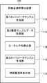
- FIG. 3 is a block diagram illustrating an example of a functional configuration of the information amount criterion calculation device 100.
- the information amount criterion calculation device 100 includes a first parameter sample generation unit 110, a second type sample data acquisition unit 112, a kernel average calculation unit 114, a second parameter sample generation unit 116, and an information amount criterion calculation unit. 118.
- the first parameter sample generator 110 is also called a prior parameter sample generator
- the kernel average calculator 114 is also called a corresponding data calculator
- the second parameter sample generator 116 is a new parameter sample generator. Also called.
- the first parameter sample generator 110 receives the input of the first type of data (data X) and outputs the second type of data (data Y), and the prior distribution of the parameter ⁇ of the regression model r (x, ⁇ )
- the sample data of the parameter ⁇ is generated based on ⁇ ( ⁇ ).
- the prior distribution ⁇ ( ⁇ ) is, for example, a uniform distribution. In the case of a uniform distribution, sample data is randomly selected from a domain in which the value of ⁇ is defined. If a distribution estimated to be close to the posterior distribution to some extent is obtained, the distribution may be set to the prior distribution ⁇ ( ⁇ ). In this case, sample data is selected from the domain according to the prior distribution ⁇ ( ⁇ ).
- the prior distribution ⁇ ( ⁇ ) is not limited to the example described above, nor is it necessarily given explicitly. If the prior distribution ⁇ ( ⁇ ) is not explicitly given, the prior distribution ⁇ ( ⁇ ) is set to, for example, a uniform distribution. In addition, as described later, the prior distribution ⁇ ( ⁇ ) may be set by the user.
- the sample data of the parameter ⁇ is expressed by the following equation. It is represented as (14).
- d ⁇ indicates the number of dimensions of the parameter (that is, the number of types of the parameter ⁇ ). That is, Expression (14) indicates that the number of sets including the parameters of d ⁇ types is m.
- R indicates a real number.
- the sample data of the parameter ⁇ is shown as a real number in the d ⁇ dimension, and follows a prior distribution ⁇ ( ⁇ ).
- the prior distribution ⁇ ( ⁇ ) is stored in the memory 102 in advance.
- the prior distribution ⁇ ( ⁇ ) is set in advance, for example, with an accuracy according to the knowledge that the user has about the simulation target.
- the second type sample data acquisition unit 112 receives the parameters ⁇ generated by the first parameter sample generation unit 110, and supplies the received m parameters ⁇ with observation data (observation data X n ) of the first type of data. To the simulator server 200. The simulator server 200 receives the m parameters ⁇ and the observation data (observation data X n ) of the first type of data.
- the simulator server 200 performs a simulation calculation based on the observation data (observation data X n ) of the first type of data for each of the input m parameters ⁇ . That is, the simulator server 200 executes m types of simulation calculations on the observation target according to the input m parameters ⁇ . The simulator server 200 executes m kinds of simulation calculations, thereby obtaining m kinds of simulation results ( ) Is calculated.
- the second type sample data acquisition unit 112 acquires m types of simulation results from the simulator server 200 as second type sample data.
- the above processing can be mathematically expressed as follows.
- the second type sample data acquisition unit 112 converts the sample data having n elements (the same number as the number of elements of the observation data Xn ) represented by Expression (15) into model data for each parameter sample data. (Simulator server 200).
- the sample data obtained by the second type sample data obtaining unit 112 is represented as an n-dimensional real number, and the likelihood function p (y
- the kernel average calculation unit 114 estimates a kernel average indicating a posterior distribution of parameters according to the kernel ABC. That is, the kernel average calculation unit 114 calculates the kernel average indicating the posterior distribution of the parameters based on the sample data of the parameters and the second type of sample data. In particular, the kernel average calculation unit 114 calculates a kernel average using a kernel function including the inverse temperature.
- the kernel ABC will be described. Using the sample data represented by the equation (14) and the sample data represented by the equation (15), the kernel ABC calculates a kernel average represented by the following equation (16).
- the kernel mean corresponds to a posterior distribution expressed on a reproducing kernel Hilbert space (RKHS) by kernel mean embedding (Kernel Mean Embeddings).
- the kernel average is an example of data corresponding to a parameter distribution (posterior distribution).
- the weight w j is represented as in the following Expression (17).
- H indicates a regenerative nuclear Hilbert space. That is, the larger the weight (importance) w j is, the larger the sample This means that the kernel has a strong effect on the average. The smaller the weight w j is, the more samples Indicates that the kernel has a small effect on the average.
- a superscript T indicates transposition of a matrix or a vector.
- I represents a unit matrix
- ⁇ (where ⁇ > 0) is a regularization constant.
- the vector k y (Y n) and the Gram matrix (Gramm Matrix) G is the kernel k y for the data vector Y n consisting of real elements, is represented by the following formula (18), formula (19) .
- k y (Y n) is the observed data Y n, proximity of the sample data of formula (15) corresponding to the observation data Y n (norm), i.e. a function for calculating the degree of similarity.
- the kernel average is a weighted average that determines the weight of each parameter using the calculated degree of similarity and is calculated according to the processing shown in Expression (16).
- Equation (18) is obtained from a plurality of pieces of observation information observed when an input is given to the observation target, and a second type of data created by the simulator server 200 for the first type of data representing a plurality of samples and inputs. It can be said that the difference from the above is calculated.
- Expression (16) also indicates a process of calculating a large weight for data similar to observed data actually observed for an observation target among m types of simulation results. You can also.
- the processing for calculating a small weight is represented. That is, it can be said that Expression (17) calculated using Expression (18) represents a process of calculating a weight according to the degree of similarity between the simulation result and the observation data. This can be said to be a process using a covariate shift.
- the distribution q 0 (x) that the training dataset ⁇ X n , Y n ⁇ follows is different from the distribution q 1 (x) that the test or prediction dataset follows.
- x) is the same.
- the covariate shift is a process of calculating y for a given x, it is constant for a plurality of x, but the distribution as an input is different between training and testing. It represents that.
- the probability densities q 0 (x) and q 1 (x) are known, or their ratio q 0 (x) / q 1 (x) is known.
- the ratio is closer to 1, it means that q 0 (x) during training and q 1 (x) during testing occur with similar probability.
- the index is not limited to the ratio, and may be any index that represents the difference between the distribution at the time of training and the distribution at the time of testing, such as the difference between the two distributions.
- Equation (20) corresponds to equation (25) described below, except for the difference in whether the inverse temperature depends on the training data (observation data).
- (Y n , Y n ′) on the left side of Expression (20) is expressed by a kernel function represented by an n-dimensional vector (a data set having n elements (that is, including n elements)).
- n-dimensional vector a data set having n elements (that is, including n elements)
- the function is a two-variable function for the second type of data. That, Y n is the left side, shows the first variable in the function of two variables, Y n 'is in the left side, shows a second variable in the function of two variables.
- the right side of the Y i indicates the i-th element of the n-dimensional vector that is input to the variable determined as the first variable.
- Y i ′ on the right side indicates the i-th element of the n-dimensional vector input to the two-variable function as the second variable.
- ⁇ is the standard deviation of Gaussian noise for the second type of data. More specifically, in equation (20), ⁇ is the standard deviation of the distribution of the entire observation data of the second type of data used for calculating equation (20). In particular, the meaning of ⁇ in equation (20) can be a value indicating a scale for measuring the similarity between the distribution of the second type of observation data and the distribution of the second type of sample data. Further, n is the number of data of the second type of data, ⁇ i is the reverse temperature, and Y i and Y i ′ are the values of the second type of data.
- each element (for example, the type of observation data) included in the second type of data set is weighted by the inverse temperature ⁇ i .
- ⁇ i the reverse temperature
- ⁇ i is the inverse temperature depending on the training data (observed data) ⁇ X i , Y i ⁇ . That is, the reverse temperature values can be set to be different for each data. That is, the inverse temperature ⁇ i can be set for each type of observation data (ie, the elements included in Y n ). For example, a larger value is set as the inverse temperature for the type of observation data with a higher importance, and a smaller value is set as the inverse temperature for the observation data with a lower importance. Therefore, ⁇ i can also be expressed as a contribution indicating the importance of the type of observation data (that is, the element included in Y n ). In other words, the inverse temperature can be said to be the contribution of each piece of observation information to the plurality of pieces of observation information.
- the kernel average is calculated for a constant inverse temperature that does not depend on the training data (observation data) ⁇ X i , Y i ⁇ .
- the kernel average calculator 114 calculates a kernel average represented by the following equation (21).
- (Y n , Y n ′) on the left side of Expression (25) is a kernel function represented by an n-dimensional vector (a data set having n elements (that is, including n elements)).
- n-dimensional vector a data set having n elements (that is, including n elements)
- the function is a two-variable function for the second type of data. That, Y n is the left side, shows the first variable in the function of two variables, Y n 'is in the left side, shows a second variable in the function of two variables.
- the right side of the Y i indicates the i-th element of the n-dimensional vector that is input to the variable determined as the first variable.
- Y i ′ on the right side indicates the i-th element of the n-dimensional vector input to the two-variable function as the second variable.
- the elements for example, the observation data
- the elements are weighted by the inverse temperature ⁇ i .
- the elements (for example, types of observation data) included in the second type of data set are weighted at a constant inverse temperature. That is, in the processing shown in the equation (25), the degree of contribution of the elements included in the second type of data set is constant.
- the contribution is assumed to be constant in this example, the contribution is not limited to a constant defined mathematically, but may be substantially constant.
- the substantially constant value indicates a value calculated by adding a noise having an average of 0 standard deviation s to the average value a. In this case, the standard deviation s is, for example, a value of about 0% to 10% of the magnitude of a.
- ⁇ is the standard deviation of Gaussian noise for the second type of data. More specifically, in Expression (25), ⁇ is a standard deviation of a distribution including the entire observation data of the second type of data used for calculating Expression (25).
- the meaning of ⁇ in equation (25) can be a value indicating a scale for measuring the similarity between the distribution of the second type of observation data and the distribution of the second type of sample data.
- n is the number of data of the second type of data
- ⁇ is the reverse temperature
- Y i and Y i ′ are the values of the second type of data.
- ⁇ is a constant that does not depend on observation data.
- the second parameter sample generator 116 generates sample data of parameters according to the posterior distribution defined using the inverse temperature based on the kernel average calculated by the kernel average calculator 114.
- the posterior distribution defined using the inverse temperature is a posterior distribution defined based on Bayes' theorem by a prior distribution and a likelihood function controlled by the inverse temperature.
- the posterior distribution is the distribution according to exp (- ⁇ nL n ( ⁇ ) + log ⁇ ( ⁇ )).
- the second parameter sample generation unit 116 generates sample data of parameters according to the posterior distribution using kernel hardening.
- kernel hardening m pieces of sample data ⁇ 1 ,..., ⁇ m according to the posterior distribution are generated by the update equations shown in the following equations (26) and (27).
- h j 0,..., M ⁇ 1.
- Argmax ⁇ h j ( ⁇ ) indicates the value of ⁇ that maximizes the value of h j ( ⁇ ).
- h j are sequentially represented by Expression (27).
- the initial values h 0 and ⁇ of h j kernel average values calculated according to the processing shown in Expression (21) are used. That is, the second parameter sample generation unit 116 uses the kernel average calculated by the kernel average calculation unit 114 and performs m processes of m pieces of sample data ⁇ suitable for representing the kernel average by a predetermined process such as kernel hardening. 1, ..., to generate the ⁇ m.
- the information amount criterion calculation device 100 executes a process of calculating m sample data according to the estimated posterior distribution for m sample data according to the prior distribution. Therefore, it can be said that the process in the information amount criterion calculation device 100 is a process of adjusting the values of m sample data.
- the information amount criterion calculation unit 118 calculates the WBIC for the model based on the parameter sample data generated by the second parameter sample generation unit 116. Specifically, the information amount criterion calculation unit 118 calculates the WBIC using the sample data of the parameters generated by the second parameter sample generation unit 116 and Expression (13).
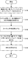
- FIG. 4 is a flowchart illustrating an example of the operation of the information amount criterion calculation device 100. Hereinafter, the operation will be described with reference to FIG.
- step S100 the first parameter sample generation unit 110 generates sample data of the parameter ⁇ based on the prior distribution ⁇ ( ⁇ ).
- the sample data generated by the first parameter sample generator 110 is input to the simulator server 200.
- the generated sample data is input to the simulator server 200 by the second type sample data acquisition unit 112, for example.
- the second type sample data acquisition unit 112 acquires the second type sample data calculated by the simulator server 200 according to the model in which the sample data generated in step S100 is set as a parameter. That is, the second type sample data acquisition unit 112, the training data set ⁇ X n, Y n ⁇ , which is obtained in advance of, the X n is a first type of data input to the model, the output from the model get.
- the training data set ⁇ X n , Y n ⁇ is information in which X n being the first type of data and Y n being the second type of data are associated with each other.
- the second type of data Yn is, for example, information obtained by actually performing processing (operation) on the first type of data Xn by the observation target.
- the simulator server 200 calculates the data Y by performing an operation according to the value represented by the parameter ⁇ on the value of the data X. Thereby, the processing (operation) in the observation target is simulated.
- the parameter ⁇ represents, for example, the relationship between input and output in each process (operation).
- step S101 the simulator server 200 receives, as an input, Xn that is a first type of data representing an input given to the observation target, and performs a process according to the input parameter ⁇ with the first type of data.
- the observation object is simulated by applying to a certain Xn .
- the simulator server 200 generates a simulation result ( ) To create.
- the processing in the simulator server 200 may be executed in advance.
- the second type sample data acquisition unit 112 reads information in which the sample data of the parameter ⁇ is associated with the simulation result calculated when the sample data is set.
- the kernel average calculation unit 114 calculates the kernel average indicating the posterior distribution of the parameters by the kernel ABC using the sample data obtained in steps S100 and S101. Note that this posterior distribution is a posterior distribution defined using the inverse temperature as described above.
- the kernel average calculation unit 114 calculates a kernel average using a kernel function including the inverse temperature represented by Expression (25). In other words, the kernel average calculation unit 114 determines the importance of each sample of the parameter according to the difference between the observation data and the sample data for the second type of data and the contribution of each observation data. , Data corresponding to the parameter distribution is calculated.
- step S103 the second parameter sample generation unit 116 generates parameter sample data according to the posterior distribution defined using the inverse temperature, based on the kernel average calculated in step S102.
- step S104 the information amount criterion calculation unit 118 calculates the WBIC for the model using Expression (13) based on the sample data of the parameters generated in step S103.
- the kernel average calculation unit 114 calculates a kernel average corresponding to the posterior distribution defined using the inverse temperature. Therefore, even when a value other than 1 is set as the value of the inverse temperature, sample data of the posterior distribution can be obtained by using a method such as kernel ABC and kernel hardening.
- the second type sample data acquisition unit 112 converts the sample data represented by Expression (15) into a model (simulator server 200) for each parameter sample data. Just get from. That is, the number of times of executing the simulation can be suppressed as compared with the case where the posterior distribution sample data is obtained by the method using MCMC. That is, according to the present embodiment, parameters can be calculated efficiently. Therefore, the WBIC can be calculated efficiently.
- the sample data generated in step S103 is used only for calculating the WBIC, but may be used for simulation by the simulator server 200. That is, the information amount criterion calculation device 100 may input the sample data generated in step S103 (that is, the sample data of the parameter ⁇ ) to the simulator server 200.
- the simulator server 200 receives the m pieces of the sample data and executes a simulation calculation on the observation target based on the received sample data. Specifically, the simulator server 200 executes m types of simulation processes on Xn that is given first type of data in accordance with the sample data. As a result, the simulator server 200 calculates m types of simulation results for the given first type of data Xn .
- the m types of simulation results are not necessarily different from each other, and may include the same results.
- the information amount criterion calculation device 100 receives m types of simulation results. Then, the information amount criterion calculation device 100 calculates a simulation result obtained by integrating the m types of simulation results. For example, the information amount criterion calculation device 100 calculates an average of m types of simulation results. That is, the information amount criterion calculation device 100 calculates a simulation result for the given first type of data Xn . The information amount criterion calculation device 100 may calculate the simulation result for the given first type of data Xn, for example, by calculating a weighted average of m types of simulation results.
- Information criterion calculation device 100 by executing the processing described above with reference to FIG. 4, and the simulation result of the simulator server 200 calculates the observation information Y n matches (conforms) manner, the parameters ⁇ Calculate sample data. Since the calculated sample data is data according to the posterior distribution, the above-described simulation result calculated by the information amount criterion calculation device 100 is a simulation result according to the sample data according to the posterior distribution. In other words, the information amount criterion calculation device 100 can calculate a simulation result that matches the observation information based on the simulation result created by the simulator server 200. Therefore, for the sample data of the parameter ⁇ given to the simulator server 200, by creating a value that matches the observation information, the information amount criterion calculation device 100 can calculate a simulation result suitable for the observation information. it can.
- Embodiment 2 a second embodiment will be described. Due to the characteristics of the kernel ABC, the WBIC calculation method described in Embodiment 1 may have a different result from the WBIC calculation using the MCMC method. This is considered to be due to the following reasons.
- ⁇ is a hyperparameter of the standard deviation of Gaussian noise in equation (3). Then, nL n ( ⁇ ) is calculated using this hyperparameter.
- ⁇ k may be larger than the true standard deviation ⁇ 0 of Gaussian noise. Due to the difference between ⁇ 0 and ⁇ k , the WBIC value calculated using the kernel ABC differs from the WBIC value calculated using the likelihood function directly, such as the MCMC method.
- ⁇ k is used instead of ⁇ 0 as a specific value of ⁇ in equation (25). Therefore, there is a possibility that an accurate WBIC value cannot be calculated in the first embodiment. is there.
- the model is modeled by a regression function involving Gaussian noise.
- ⁇ 0 can be said to be the value of the standard deviation of the Gaussian noise with respect to the regression function.
- ⁇ k can be said to be a value indicating a scale for measuring the similarity between the distribution of the second type of observation data and the distribution of the second type of sample data.
- Embodiment 1 a method for calculating WBIC more accurately than the method for calculating WBIC shown in Embodiment 1 will be described.
- the standard deviation ⁇ 0 of Gaussian noise is known. That is, before performing the correction described below, the standard deviation ⁇ 0 of the Gaussian noise is estimated by a known method and is known.
- Equation (7) F n ( ⁇ ) rather than to be expressed as F n ( ⁇ , ⁇ ).
- ⁇ and ⁇ mean variables. such as beta 1, code subscript is given to beta represents a specific constant. Similarly, a code with a subscript attached to ⁇ , such as ⁇ 0 , indicates a specific constant.
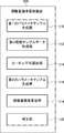
- FIG. 5 is a block diagram illustrating an example of a functional configuration of the information amount criterion calculation device 300 according to the second embodiment.
- the information amount criterion calculation device 300 is different from the information amount criterion calculation device 100 according to the first embodiment in further including a correction unit 120.
- the information amount criterion calculation device 300 also has a hardware configuration as shown in FIG. 2 similarly to the information amount criterion calculation device 100, and the processor 103 reads out software from the memory 102 and executes the software. The processing of each configuration shown in FIG.
- the correction unit 120 corrects the WBIC calculated by the information amount criterion calculation unit 118.
- the correction unit 120 performs correction using the fact that different ⁇ s are represented by different inverse temperatures ⁇ in the relational expressions derived from Expressions (7) and (3).
- the relationship of F n ( ⁇ , ⁇ ) between different ⁇ and ⁇ is represented by the following equation (28).
- Equation (28) C k and ⁇ k are defined as shown in the following equations (29) and (30). ⁇ Equation (29)>
- Equation (28) is a WBIC when the inverse temperature value in equation (7) is 1 and the standard deviation value is ⁇ k, and the inverse temperature value in equation (7) is a predetermined value ⁇ other than 1 It shows the relationship with WBIC when k is set and the value of the standard deviation is set to ⁇ 0 .
- Expression (7) is an expression obtained by expanding the definition expression of Bayes free energy so as to include the inverse temperature.
- the correction unit 120 corrects the WBIC calculated by the information amount criterion calculation unit 118 using the relationship represented by Expression (28). Specifically, the correction unit 120 performs the correction by one of the two correction methods described below.
- F n ( ⁇ , ⁇ ) that is, an asymptotically developed mathematical expression of the mathematical expression (7) is shown.
- Equation (31) is an equation asymptotically expanded for F n ( ⁇ , ⁇ ).
- the correction unit 120 calculates the relationship expressed by excluding the real logarithmic threshold ⁇ obtained from the two mathematical expressions in which different values of ⁇ are set in Expression (31), and the relationship expressed by Expression (28). Is used, the WBIC calculated by the information amount criterion calculation unit 118 is corrected. Since the relationship excluding the real logarithmic threshold ⁇ is used, the first method can correct the value without calculating the real logarithmic threshold ⁇ , which is generally difficult to calculate.
- the relational expression indicating the relationship expressed by excluding the real logarithmic threshold value ⁇ is obtained by deleting the term of the real logarithmic threshold value ⁇ from the simultaneous equations including Expressions (32) and (33).
- the entropy (minus log likelihood function) L n ( ⁇ 0 ) is (However, Is sufficiently approximated by the average (posterior mean) calculated from the sample data of the parameters according to the posterior distribution, the following equation (34) is satisfied.
- Expression (34) is obtained by a relational expression indicating a relationship expressed by excluding the real logarithmic threshold value ⁇ and a relational expression expressed by Expression (28).
- F n (1, ⁇ k ) corresponds to the WBIC calculated by the information amount criterion calculation unit 118. Therefore, the correction unit 120 generates the post-correction WBIC from the pre-correction WBIC calculated by the information amount criterion calculation unit 118 by calculating Expression (34). In other words, the correction unit 120 calculates the first type of data (that is, the input to the observation target) and the observation information observed with respect to the observation target in the case of the first type regarding the parameter set according to the estimated posterior distribution.
- the correction unit 120 may perform the correction by the above-described first correction method. However, when the calculation by approximation of L n ( ⁇ 0 ) cannot be performed, the first correction method cannot be used. In this case, the correction unit 120 may perform the correction by the second correction method.
- the correction unit 120 calculates the relationship expressed by excluding the real logarithmic threshold value and entropy obtained from three mathematical expressions in which different values of ⁇ are set in Expression (31), and Expression (28)
- the WBIC calculated by the information amount criterion calculation unit 118 is corrected by using the relationship indicated by. Since not only the real logarithmic threshold but also the relationship from which entropy is excluded is used, the second correction method can correct even if calculation by approximation of L n ( ⁇ 0 ) is not possible.
- the correction unit 120 can calculate the corrected WBIC F n (1, ⁇ 0 ). This is because the value of F n ( ⁇ 1 , ⁇ 0 ) can be calculated as the value of F n (1, ⁇ 1 ), and the value of F n ( ⁇ 2 , ⁇ 0 ) is F n (1, ⁇ 0 ). This is because it can be calculated as the value of ⁇ 2 ) (see equation (28)). That is, F n ( ⁇ 1 , ⁇ 0 ) and F n ( ⁇ 2 , ⁇ 0 ) are the two uncorrected WBICs calculated by the information amount criterion calculation unit 118.
- the correction unit 120 calculates the corrected WBIC from the WBIC calculated by the information amount criterion calculation unit 118 by calculating Expression (38).
- the information amount criterion calculation unit 118 calculates the WBIC for each of two different contributions (reverse temperatures), and the correction unit 120 causes the information amount criterion calculation unit 118 It can also be said that a description is given of a process of calculating a weighted average according to the degree of contribution (reverse temperature) for the calculated WBIC.
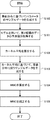
- FIG. 6 is a flowchart illustrating an example of the operation of the information amount criterion calculation device 300.
- the flowchart shown in FIG. 6 differs from the flowchart shown in FIG. 4 in that step S105 is added after step S104.
- step S105 is added after step S104.
- step S104 the process proceeds to step S105.
- the correction unit 120 corrects the WBIC before correction calculated in step S104 according to the above-described first correction method or second correction method.
- step S102 when the correction is performed by the second correction method, two types of kernel averages are calculated in step S102. One is the kernel average calculated by the kernel average calculation unit 114 using ⁇ 1 as ⁇ in equation (25), and the other is the kernel average calculation unit 114 using ⁇ 2 as ⁇ in equation (25) This is the kernel average calculated as follows.
- step S103 parameter sample data is generated for each of the two types of kernel averages.
- step S104 two WBICs are calculated in step S104 using the two sets of sample data generated in step S103.
- WBIC is corrected by correction section 120. Therefore, a more accurate WBIC value can be obtained.
- FIG. 7 is a block diagram illustrating a configuration of the information processing device 1.
- the information processing device 1 includes a correspondence data calculation unit 2 and a new parameter sample generation unit 3.
- the correspondence data calculation unit 2 calculates a plurality of pieces of observation information (Y n ) observed when an input (X n ) is given to the observation target and a second type of data (Y n ). ) And the contribution ( ⁇ ) of each piece of observation information to the plurality of pieces of observation information, the importance of each sample of the parameter is determined.
- the second type of data is data created by a simulator that simulates an observation target based on a sample of parameters for a plurality of samples and the first type of data representing the input. Then, the correspondence data calculation unit 2 calculates data corresponding to the parameter distribution.
- the new parameter sample generation unit 3 generates a new parameter sample according to a predetermined process (for example, kernel hardening) using data corresponding to the parameter distribution calculated by the correspondence data calculation unit 2. According to such a configuration, the information processing device 1 can efficiently calculate the parameters.
- a predetermined process for example, kernel hardening
- Appendix 1 A plurality of observation information observed when an input is given to an observation target, and a simulator that simulates the observation target based on a sample of parameters is created for a plurality of the samples and a first type of data representing the input. Corresponding data for determining the importance of each sample according to the difference from the second type of data and the degree of contribution of each observation information in the plurality of observation information, and calculating data corresponding to the parameter distribution Calculating means;
- An information processing apparatus comprising: a new parameter sample generation unit configured to generate a new sample of the parameter according to a predetermined process using data corresponding to the distribution of the parameter.
- the data corresponding to the distribution of the parameters is a kernel mean
- the correspondence data calculation means calculates the kernel average using a kernel function including the degree of contribution as an inverse temperature, 4.
- the information processing apparatus according to claim 1 wherein the new parameter sample generation unit generates the sample using the kernel average calculated by the correspondence data calculation unit.
- the correspondence data calculation means calculates the kernel average by a kernel ABC (Kernel Approximate Bayesian Computation) using the kernel function represented by the following equation.
- ⁇ is the standard deviation of Gaussian noise for the second type of data
- n is the number of elements of the second type of data
- ⁇ is the inverse temperature
- Y i and Y i ′ is the value of the second type of data.
- the correction means is a relation expressed by excluding a real logarithmic threshold, which is obtained from two mathematical expressions in which different inverse temperature values are set in a second mathematical expression which is an asymptotically developed mathematical expression of the first mathematical expression.
- the information processing device according to claim 7, wherein the WBIC calculated by the information amount criterion calculating unit is corrected by using a certain second relationship and the first relationship.
- the correction means is expressed by excluding a real logarithmic threshold and entropy obtained from three mathematical expressions in which different inverse temperature values are set in a second mathematical expression which is an asymptotically developed mathematical expression of the first mathematical expression.
- the information processing device wherein the WBIC calculated by the information amount criterion calculation unit is corrected by using a third relationship, which is a relationship, and the first relationship. (Appendix 10) Using the input and the observation information when the input is given, a likelihood of the new sample calculated by the new parameter sample generation unit is calculated, and the WBIC is calculated based on the calculated likelihood. 4.
- the information processing device further comprising: a correction unit configured to perform correction.
- a correcting unit for correcting the WBIC The information amount criterion calculation means calculates the WBIC for each of two different contributions, and the correction means calculates a weight according to the contribution for the WBIC calculated by the information amount criterion calculation means.
- the information processing device which calculates an average.
- Appendix 12 An information processing apparatus according to any one of Supplementary Notes 1 to 11, and the simulator, The information processing system, wherein the simulator executes a process based on the sample generated by the new parameter sample generation unit.
- Appendix 13 Depending on the information processing device, A plurality of observation information observed when an input is given to an observation target, and a simulator that simulates the observation target based on a sample of parameters is created for a plurality of the samples and a first type of data representing the input.
- Corresponding data for determining the importance of each sample according to the difference from the second type of data and the degree of contribution of each observation information in the plurality of observation information, and calculating data corresponding to the parameter distribution A calculating step;
- a non-transitory computer-readable medium storing a program for causing a computer to execute a new parameter sample generating step of generating a new sample of the parameter according to a predetermined process using data corresponding to the parameter distribution.
Landscapes
- Engineering & Computer Science (AREA)
- General Physics & Mathematics (AREA)
- Physics & Mathematics (AREA)
- Automation & Control Theory (AREA)
- Business, Economics & Management (AREA)
- Environmental & Geological Engineering (AREA)
- Strategic Management (AREA)
- Human Resources & Organizations (AREA)
- Economics (AREA)
- Evolutionary Computation (AREA)
- Artificial Intelligence (AREA)
- Life Sciences & Earth Sciences (AREA)
- Atmospheric Sciences (AREA)
- Biodiversity & Conservation Biology (AREA)
- Ecology (AREA)
- Environmental Sciences (AREA)
- Medical Informatics (AREA)
- Health & Medical Sciences (AREA)
- Computer Vision & Pattern Recognition (AREA)
- Software Systems (AREA)
- Game Theory and Decision Science (AREA)
- Development Economics (AREA)
- Entrepreneurship & Innovation (AREA)
- Marketing (AREA)
- Operations Research (AREA)
- Quality & Reliability (AREA)
- Tourism & Hospitality (AREA)
- General Business, Economics & Management (AREA)
- Theoretical Computer Science (AREA)
- Management, Administration, Business Operations System, And Electronic Commerce (AREA)
Abstract
効率的にパラメータを算出する。情報処理装置(1)は、観測対象に入力を与えた場合に観測される複数の観測情報と、前記観測対象をパラメータのサンプルに基づきシミュレーションするシミュレータが複数の前記サンプル及び前記入力を表す第1種類のデータに対して作成した第2種類のデータとの差異と、前記複数の観測情報における各観測情報の寄与度とに応じて、各前記サンプルの重要度を決定し、前記パラメータの分布に対応するデータを算出する対応データ算出部(2)と、前記パラメータの分布に対応するデータを用いて、所定の処理に従い、前記パラメータの新たなサンプルを生成する新規パラメータサンプル生成部(3)とを備える。
Description
本発明は情報処理装置、情報処理方法、及びプログラムに関する。
予測モデルを用いた数値予測、および、この予測モデルの学習に関連して幾つかの技術が提案されている。
例えば、特許文献1には、気象予測モデルを用いて定期的に気象予測を行う気象予測システムが記載されている。この気象予測システムは、気象予測モデルに観測データを同化して気象予測を行い、気象予測の演算に用いる演算パラメータを予測時刻に応じて変更する。
例えば、特許文献1には、気象予測モデルを用いて定期的に気象予測を行う気象予測システムが記載されている。この気象予測システムは、気象予測モデルに観測データを同化して気象予測を行い、気象予測の演算に用いる演算パラメータを予測時刻に応じて変更する。
また、特許文献2に記載の予測装置は、複数の予測モデルを作成し、予測モデルそれぞれに対して残差を予測する残差予測モデルを作成する。そして、この予測装置は、予測モデル毎の予測値に対して、残差予測モデルによる残差予測値を合成して、予測装置としての予測値を算出する。
しかし、特許文献1に開示されたシステム、及び、特許文献2に開示された装置を用いたとしても、高精度な予測を効率的に実行することはできない。この理由は、予測モデルにおけるパラメータを効率的に決めることができないからである。
そこで、本明細書に開示される実施形態が達成しようとする目的の1つは、効率的にパラメータを算出することができる情報処理装置等を提供することにある。
第1の態様にかかる情報処理装置は、
観測対象に入力を与えた場合に観測される複数の観測情報と、前記観測対象をパラメータのサンプルに基づきシミュレーションするシミュレータが複数の前記サンプル及び前記入力を表す第1種類のデータに対して作成した第2種類のデータとの差異と、前記複数の観測情報における各観測情報の寄与度とに応じて、各前記サンプルの重要度を決定し、前記パラメータの分布に対応するデータを算出する対応データ算出手段と、
前記パラメータの分布に対応するデータを用いて、所定の処理に従い、前記パラメータの新たなサンプルを生成する新規パラメータサンプル生成手段と
を備える。
観測対象に入力を与えた場合に観測される複数の観測情報と、前記観測対象をパラメータのサンプルに基づきシミュレーションするシミュレータが複数の前記サンプル及び前記入力を表す第1種類のデータに対して作成した第2種類のデータとの差異と、前記複数の観測情報における各観測情報の寄与度とに応じて、各前記サンプルの重要度を決定し、前記パラメータの分布に対応するデータを算出する対応データ算出手段と、
前記パラメータの分布に対応するデータを用いて、所定の処理に従い、前記パラメータの新たなサンプルを生成する新規パラメータサンプル生成手段と
を備える。
第2の態様にかかる情報処理方法は、
情報処理装置によって、
観測対象に入力を与えた場合に観測される複数の観測情報と、前記観測対象をパラメータのサンプルに基づきシミュレーションするシミュレータが複数の前記サンプル及び前記入力を表す第1種類のデータに対して作成した第2種類のデータとの差異と、前記複数の観測情報における各観測情報の寄与度とに応じて、各前記サンプルの重要度を決定し、前記パラメータの分布に対応するデータを算出し、
前記パラメータの分布に対応するデータを用いて、所定の処理に従い、前記パラメータの新たなサンプルを生成する。
情報処理装置によって、
観測対象に入力を与えた場合に観測される複数の観測情報と、前記観測対象をパラメータのサンプルに基づきシミュレーションするシミュレータが複数の前記サンプル及び前記入力を表す第1種類のデータに対して作成した第2種類のデータとの差異と、前記複数の観測情報における各観測情報の寄与度とに応じて、各前記サンプルの重要度を決定し、前記パラメータの分布に対応するデータを算出し、
前記パラメータの分布に対応するデータを用いて、所定の処理に従い、前記パラメータの新たなサンプルを生成する。
第3の態様にかかるプログラムは、
観測対象に入力を与えた場合に観測される複数の観測情報と、前記観測対象をパラメータのサンプルに基づきシミュレーションするシミュレータが複数の前記サンプル及び前記入力を表す第1種類のデータに対して作成した第2種類のデータとの差異と、前記複数の観測情報における各観測情報の寄与度とに応じて、各前記サンプルの重要度を決定し、前記パラメータの分布に対応するデータを算出する対応データ算出ステップと、
前記パラメータの分布に対応するデータを用いて、所定の処理に従い、前記パラメータの新たなサンプルを生成する新規パラメータサンプル生成ステップと
をコンピュータに実行させる。
観測対象に入力を与えた場合に観測される複数の観測情報と、前記観測対象をパラメータのサンプルに基づきシミュレーションするシミュレータが複数の前記サンプル及び前記入力を表す第1種類のデータに対して作成した第2種類のデータとの差異と、前記複数の観測情報における各観測情報の寄与度とに応じて、各前記サンプルの重要度を決定し、前記パラメータの分布に対応するデータを算出する対応データ算出ステップと、
前記パラメータの分布に対応するデータを用いて、所定の処理に従い、前記パラメータの新たなサンプルを生成する新規パラメータサンプル生成ステップと
をコンピュータに実行させる。
上述の態様によれば、効率的にパラメータを算出することができる情報処理装置等を提供することができる。
以下の各実施形態においては、理解しやすさのため数学的な用語を用いて説明するが、各用語は必ずしも数学的に定義されている値でなくてもよい。たとえば、距離は、ユークリッドノルムや、1ノルム等、数学的に定義することができる。しかし、距離は、そのような値に1を足したような値であってもよい。すなわち、以下の実施形態にて用いられる用語は、数学的に定義されている用語でなくてもよい。
<実施の形態1>
以下、図面を参照して本発明の実施の形態について説明する。
図1は、実施形態に係る情報処理システム10の構成の一例を示すブロック図である。図1に示すように、情報処理システム10は、情報量規準算出装置100とシミュレータサーバ(シミュレータ)200とを備える。なお、情報量規準算出装置100は情報処理装置と称されることがある。
以下、図面を参照して本発明の実施の形態について説明する。
図1は、実施形態に係る情報処理システム10の構成の一例を示すブロック図である。図1に示すように、情報処理システム10は、情報量規準算出装置100とシミュレータサーバ(シミュレータ)200とを備える。なお、情報量規準算出装置100は情報処理装置と称されることがある。
シミュレータサーバ200は、第1種類のデータの入力を受けて第2種類のデータを出力するシミュレータである。すなわち、シミュレータサーバ200は、パラメータθにより規定されるモデルに従って、第1種類のデータから、第2種類のデータを予測するシミュレーション処理を行なう。たとえば、シミュレータサーバ200は、パラメータθのサンプルに基づき、観測対象における処理(動作)をシミュレーションする処理を実行する。サンプルは、パラメータθの値を表す。したがって、複数のサンプルは、当該パラメータθの値として設定される複数の例(データ)を表している。
以下では、第1種類のデータをデータXと称し、第2種類のデータをデータYと称する。また、観測データの個数をn(nは正の整数)として、データXの観測データ(第1種類の観測データ)を観測データXnと表記し、データYの観測データ(第2種類の観測データ)を観測データYnと表記する。また、観測データXnの要素をX1、・・・、Xnと表記し、観測データYnの要素をY1、・・・、Ynと表記する。情報量規準算出装置100は、データXi(iは、1≦i≦nの整数)とデータYiとが一対一に対応付けられた観測データ(従って、X-Y平面にプロット可能な観測データ)を取得する。
以降においては、観測データを観測情報と表すこともある。また、観測データYnを複数の観測情報と表すこともある。この場合に、また、各要素Y1、・・・、Ynを、それぞれ、観測情報と表すこともある。
観測データXnおよびYnは特定の種類のデータに限定されず、実測されたいろいろなデータとすることができる。観測データを得るための実測方法は特定の方法に限定されず、ユーザなど人による計数または測定、あるいはセンサを用いたセンシングなど、いろいろな方法を採用可能である。
例えば、観測データXnの要素は、観測対象を構成している構成要素の状態を表すものであってもよい。観測データYnの要素は、センサ等を用いて観測対象に関して観測された状態を表すものであってもよい。例えばユーザが、製造工場の生産性を分析したい場合、観測データXnは、当該製造工場における各設備の稼働状況を表すものであってもよい。観測データYnは、複数の設備によって構成されるラインにて製造される製品の個数を表すものであってもよい。また、観測データXnは、製造工場において製品の原材料となる素材を表していてもよい。この場合に、観測データXnによって表されている素材は、1つ以上の加工工程を経て製品に加工される。当該製品は、1種類の製品であるとは限らず、複数の製品(たとえば、製品A、製品B、副産物C)であってもよい。観測データYnは、たとえば、製品Aの個数、製品Bの個数、及び、副産物Cの個数(または、生産量等)を表している。
観測対象、および、観測データは、上述した例に限定されず、たとえば、加工工場における設備であってもよいし、ある施設を建設する場合における建設システムであってもよい。
ここで、観測データXnおよびYnは、独立に同一の真の分布q(x,y)=q(x)q(y|x)に従って生じる。真のモデルq(y|x)を推測するための統計モデルは、p(y|x,θ)と表せる。q(y|x)は、事象xが生じたときに、事象yが生じる確率を表している。また、「q(x)q(y|x)」は、「q(x)×q(y|x)」を表している。以降においては、説明の便宜上、数学的な慣習に倣い、掛け算を表す演算子「×」を省略して表す。
シミュレータサーバ200が用いる回帰モデルr(x,θ)は、パラメータθの値の設定、および、変数xへのデータXの値の入力を受けて、データYの値を出力する。たとえば、シミュレータサーバ200は、データX(xの値)に対して、パラメータθのサンプルを含む演算を施すことにより、データYの値を出力する。なお、モデルには、必ずしも微分可能な関数が用いられなくてもよい。シミュレータサーバ200は、観測対象における処理又は動作をシミュレーションする。
たとえば、観測対象が製造工場である場合に、シミュレータサーバ200は、データXの値に対して、パラメータθが表す値に従った演算を施すことによってデータYを算出することによって、製造工場における各プロセスをシミュレーションする。この場合に、パラメータθは、たとえば、各プロセスにおける入出力間の関係性を表している。パラメータθは、プロセスにおける状態を表しているともいうことができる。パラメータθは、1つであるとは限らず、複数であってもよい。すなわち、回帰モデルr(x,θ)は、シミュレータサーバ200が実行している全体の処理を、符号rを用いて総称的に表しているということもできる。
ところで、モデルの良さを評価する規準として、WBIC(Widely Applicable Bayesian Information Criterion)が知られている。例えば、複数のモデルの中から適切なモデルを選択する際に、各モデルのWBICを算出することにより、どのモデルが適切であるかを調べることができる。WBICは、ベイズ自由エネルギー(Bayes free energy)を用いた情報量規準の一種である。統計モデルが特異モデル(singular model)である場合、WBICは、ベイズ自由エネルギー事象を漸近的に近似し、統計モデルが正則モデル(regular model)である場合、BIC(Bayesian Information Criterion)に一致する。ベイズ自由エネルギーは、以下の式(1)で定義される。なお、π(θ)は、パラメータθについての事前分布である。
<式(1)>

ここで、ベイズの統計的推論における表記について定義する。マイナス対数尤度関数(minus log likelihood function)Ln(θ)は以下の式(2)のように定義される。
<式(2)>

回帰問題がガウスノイズを伴う回帰関数でモデル化される場合、統計モデル(尤度関数)p(y|x,θ)は、以下の式(3)のように表される。統計モデルp(y|x,θ)は、回帰モデルr(x,θ)についての統計的な性質を示すモデルである。ただし、この回帰モデルr(x,θ)は、必ずしも、数学的な式を用いて明示的に表されているとは限らず、たとえば、xと、θとを入力として、r(x,θ)を出力とするシミュレーション等の処理を表していてもよい。一般的に、回帰モデルでは、与えられたデータに合うように数式の係数が決められる。しかし、本実施形態における回帰モデルr(x,θ)は、そのような数式が与えられていない場合であってもよい。すなわち、本実施形態における回帰モデルr(x,θ)は、入力x及びθと、出力r(x,θ)とが関連付けされた情報を表していればよい。
<式(3)>

ここで、σ(ただし、σ>0)は、ガウスノイズの標準偏差である。すなわち、σはガウスノイズを伴う回帰関数で定義されるモデルにおける当該ガウスノイズの標準偏差である。また、r(x,θ)は、シミュレータサーバ200が、回帰モデルによって表す処理に従い算出する値である。dはXの次元数(すなわち、上述した観測データの個数)である。expは、ネイピア数を底とする指数関数を表す。||は、ノルムを算出することを表す。πは、円周率を表す。
WBICは、以下の式(4)のように定義される。ここで、

は、θの事後分布の期待値である。β(ただし、β>0)は、逆温度と呼ばれるパラメータである。
<式(4)>

任意の積分可能な関数G(θ)に対し、θの事後分布の期待値は、以下の式(5)のように表すことができる。
<式(5)>

したがって、式(5)において、G(θ)に、nLn(θ)を代入した上で、式(5)の右辺を計算すれば、WBICを算出可能である。しかしながら、尤度関数p(y|x,θ)が解析的に数式として表現できない場合、すなわち尤度関数p(y|x,θ)が微分できない場合、式(5)の右辺は算出できない。
ところで、以下の式(6)に示されるWBICの漸近的な特性が知られている。
<式(6)>

式(6)、統計モデルが特異モデルであるか正則モデルであるかにかかわらず、成り立つ。なお、

は、ランダウの記号である。したがって、nが十分大きければ、ラウダウの記号で示される項は、無視することができる。つまり、ベイズ自由エネルギーは、WBICで近似される。
式(6)が成り立つことを説明する。まず、以下の式(7)で表される関数Fn(β)を定義する。
<式(7)>

<式(7)>
Fn(β)を上記のように定義すると、ベイズ自由エネルギーは以下の式(8)のように表すことができる。
<式(8)>

したがって、式(7)は、逆温度を含むようにベイズ自由エネルギーの定義式を拡張した数式である。
また、Fn(β)をβについて微分することにより得られる関数F’n(β)は、以下の式(9)のように表すことができる。
また、Fn(β)をβについて微分することにより得られる関数F’n(β)は、以下の式(9)のように表すことができる。
<式(9)>

したがって、式(4)及び式(9)から、F’n(β)=WBICが成り立つことがわかる。また、WBICの定義式を漸近展開した式として、以下の式(10)が知られている。
<式(10)>

なお、式(10)において、β=β0/log nである。ただし、β0は、正定数である。また、λは、実対数閾値(RLCT:real log canonical threshold)である。そして、θ0は、統計モデルの真のパラメータ、すなわち、q(y|x)=p(y|x,θ0)を満たすパラメータである。
一方、ベイズ自由エネルギーの定義式を漸近展開した式として、以下の式(11)が知られている。
<式(11)>

よって、これらの式から、式(6)が成り立つことが示される。
また、式(7)の定義と式(6)とから、以下の式(12)が成り立つ。なお、式(12)において、β=1/log nである。
また、式(7)の定義と式(6)とから、以下の式(12)が成り立つ。なお、式(12)において、β=1/log nである。
<式(12)>

次に、WBICの算出について説明する。
上述の通り、尤度関数p(y|x,θ)が解析的に数式として表現できない場合、すなわち尤度関数p(y|x,θ)が微分できない場合、式(5)の右辺は算出できない。そのような場合には、第2種類のデータを予測するモデルのパラメータθの事後分布に従うサンプルデータを用いて、以下の式(13)を計算することによりWBICを算出できることが知られている。なお、式(13)において、事後分布に従うサンプルデータは、

と表されている。また、jは、1≦j≦mを満たす整数であり、mは、事後分布に従うサンプルデータの数である。
上述の通り、尤度関数p(y|x,θ)が解析的に数式として表現できない場合、すなわち尤度関数p(y|x,θ)が微分できない場合、式(5)の右辺は算出できない。そのような場合には、第2種類のデータを予測するモデルのパラメータθの事後分布に従うサンプルデータを用いて、以下の式(13)を計算することによりWBICを算出できることが知られている。なお、式(13)において、事後分布に従うサンプルデータは、
<式(13)>

一般的に事後分布は不明である。このため、事後分布に従うサンプルを取得する所定の技術を利用することが求められる。事後分布に従うサンプルを取得する代表的な方法として、メトロポリス・ヘイスティングスアルゴリズムなどのMCMC(Markov Chain Monte Carlo method:マルコフ連鎖モンテカルロ法)を用いた方法が知られている。この方法では、MCMCによりパラメータθの事後分布p(θ|Xn,Yn)∝exp(-βnLn(θ)+logπ(θ))に従う、パラメータθのm個のサンプルデータを取得する。「∝」は、比例関係を表している。
しかしながら、MCMCを用いたサンプルの取得の場合、m個のθのサンプルデータを得るために、その数倍のシミュレーション(すなわち、モデルによる第2種類のデータの予測)を行なわなければならない。このため、多くの計算コストを要することとなる。
これに対し、本実施の形態では、カーネルABC(Kernel Approximate Bayesian Computation)及び所定の処理(カーネルハーディング(Kernel Herding)等)を用いてパラメータθのサンプルデータを取得する。
カーネルABCは、カーネル平均を算出することにより、事後分布を推定するアルゴリズムである。カーネルABCでは、m個のサンプルデータに基づきシミュレーションを行い、m個のパラメータのサンプルデータの重み(重要度)を、観測対象に対して観測された観測データに基づき決定することで事後分布が得られる。たとえば、シミュレーション結果が観測データに類似しているほど、当該シミュレーション結果に用いられたパラメータを重視する重みを算出する。逆に、シミュレーション結果が観測データに類似していないほど、当該シミュレーション結果に用いられたパラメータを軽視する重みを算出する。
カーネルハーディング(所定の処理の一例)は、事後分布を示すカーネル平均から事後分布に従ったサンプルを取得するアルゴリズムである。カーネルハーディングは、求めたカーネル平均に最も近くなる場合のサンプルを逐次的に決めていく。本実施形態においては、カーネルABC、及び、カーネルハーディングにおける処理によって、m個のサンプルに対して、新たにm個のサンプルが算出されるため、サンプルの値を調整しているともいうことができる。
カーネルハーディングは、サンプルを逐次的に決めていく方法であるが、事後分布(本実施形態では、推定された事後分布)に従ったサンプルを取得する所定の処理は、カーネルハーディングに限定されない。すなわち、所定の処理は、事後分布(本実施形態では、推定された事後分布)に従ったサンプルを作成する方法であればよい。
カーネルABC及び上記所定の処理(例えばカーネルハーディング)を用いてパラメータθのサンプルデータを取得する場合、m個のθのサンプルデータを得るために、m回のシミュレーション(すなわち、モデルによる第2種類のデータの予測)を行なえばよい。このため、計算コストを抑制することができる。特に、本実施の形態では、逆温度βが含まれる事後分布に従ったパラメータθのサンプルデータをカーネルABC及びカーネルハーディングを用いて取得し、そのサンプルデータに基づいてWBICを算出する情報量規準算出装置100について示す。
逆温度βは、事後分布を推定する処理において、各サンプルに基づき算出される分布が当該推定される分布に与える影響を平準化するレベルを表している値を表しているということもできる。この場合に、逆温度βが高い値であるほど、平準化するレベルは低い。言い換えると、逆温度βが高い値であるほど、推定される分布は、個々の分布の影響を受けやすくなる。これに対して、逆温度βが低い値であるほど、平準化するレベルは高い。言い換えると、逆温度βが低い値であるほど、推定される分布は、一部の分布の影響を受けにくくなる。
以下、情報量規準算出装置100について具体的に説明する。
図2は、情報量規準算出装置100のハードウェア構成の一例を示すブロック図である。情報量規準算出装置100は、入出力インタフェース101、メモリ102、及びプロセッサ103を含む。
図2は、情報量規準算出装置100のハードウェア構成の一例を示すブロック図である。情報量規準算出装置100は、入出力インタフェース101、メモリ102、及びプロセッサ103を含む。
入出力インタフェース101は、データの入出力を行うインタフェースである。例えば、入出力インタフェース101は、他の装置と通信するために使用される。この場合、例えば、入出力インタフェース101は、シミュレータサーバ200と通信するために使用される。入出力インタフェース101は、観測データXn又は観測データYnを出力するセンサ装置などの外部装置と通信するために使用されてもよい。また、入出力インタフェース101は、さらに、キーボード及びマウスなどの入力デバイスと接続するインタフェースを含んでもよい。この場合、入出力インタフェース101は、ユーザの操作により入力されたデータを取得する。また、入出力インタフェース101は、さらに、ディスプレイと接続するインタフェースを含んでもよい。この場合、例えば、入出力インタフェース101を介して、ディスプレイに、情報量規準算出装置100の演算結果などが表示される。
メモリ102は、例えば、揮発性メモリ及び不揮発性メモリの組み合わせによって構成される。メモリ102は、情報量規準算出装置100の処理に用いられる各種データの他、プロセッサ103により実行される、1以上の命令を含むソフトウェア(コンピュータプログラム)などを格納するために使用される。
プロセッサ103は、メモリ102からソフトウェア(コンピュータプログラム)を読み出して実行することで、後述する図3に示される各構成の処理を行う。プロセッサ103は、例えば、マイクロプロセッサ、MPU(Micro Processor Unit)、又はCPU(Central Processing Unit)などであってもよい。プロセッサ103は、複数のプロセッサを含んでもよい。
また、上述したプログラムは、様々なタイプの非一時的なコンピュータ可読媒体(non-transitory computer readable medium)を用いて格納され、コンピュータに供給することができる。非一時的なコンピュータ可読媒体は、様々なタイプの実体のある記録媒体(tangible storage medium)を含む。非一時的なコンピュータ可読媒体の例は、磁気記録媒体(例えばフレキシブルディスク、磁気テープ、ハードディスクドライブ)、光磁気記録媒体(例えば光磁気ディスク)、CD-ROM(Read Only Memory)CD-R、CD-R/W、半導体メモリ(例えば、マスクROM、PROM(Programmable ROM)、EPROM(Erasable PROM)、フラッシュROM、RAM(Random Access Memory))を含む。また、プログラムは、様々なタイプの一時的なコンピュータ可読媒体(transitory computer readable medium)によってコンピュータに供給されてもよい。一時的なコンピュータ可読媒体の例は、電気信号、光信号、及び電磁波を含む。一時的なコンピュータ可読媒体は、電線及び光ファイバ等の有線通信路、又は無線通信路を介して、プログラムをコンピュータに供給できる。
また、上述したプログラムは、様々なタイプの非一時的なコンピュータ可読媒体(non-transitory computer readable medium)を用いて格納され、コンピュータに供給することができる。非一時的なコンピュータ可読媒体は、様々なタイプの実体のある記録媒体(tangible storage medium)を含む。非一時的なコンピュータ可読媒体の例は、磁気記録媒体(例えばフレキシブルディスク、磁気テープ、ハードディスクドライブ)、光磁気記録媒体(例えば光磁気ディスク)、CD-ROM(Read Only Memory)CD-R、CD-R/W、半導体メモリ(例えば、マスクROM、PROM(Programmable ROM)、EPROM(Erasable PROM)、フラッシュROM、RAM(Random Access Memory))を含む。また、プログラムは、様々なタイプの一時的なコンピュータ可読媒体(transitory computer readable medium)によってコンピュータに供給されてもよい。一時的なコンピュータ可読媒体の例は、電気信号、光信号、及び電磁波を含む。一時的なコンピュータ可読媒体は、電線及び光ファイバ等の有線通信路、又は無線通信路を介して、プログラムをコンピュータに供給できる。
図3は、情報量規準算出装置100の機能構成の一例を示すブロック図である。情報量規準算出装置100は、第1のパラメータサンプル生成部110と、第2種類サンプルデータ取得部112と、カーネル平均算出部114と、第2のパラメータサンプル生成部116と、情報量規準算出部118とを有する。なお、第1のパラメータサンプル生成部110は、事前パラメータサンプル生成部とも称され、カーネル平均算出部114は対応データ算出部とも称され、第2のパラメータサンプル生成部116は、新規パラメータサンプル生成部とも称される。
第1のパラメータサンプル生成部110は、第1種類のデータ(データX)の入力を受けて第2種類のデータ(データY)を出力する回帰モデルr(x,θ)のパラメータθの事前分布π(θ)に基づいて、パラメータθのサンプルデータを生成する。事前分布π(θ)は、たとえば、一様分布である。一様分布である場合には、θの値が定義されている定義域からランダムにサンプルデータが選ばれる。ある程度事後分布に近いと推定される分布が得られている場合には、当該分布を事前分布π(θ)に設定してもよい。この場合には、当該定義域から、事前分布π(θ)に従いサンプルデータが選ばれる。事前分布π(θ)は、上述した例に限定されず、また、陽に与えられているとも限らない。事前分布π(θ)が陽に与えられていない場合には、事前分布π(θ)を、たとえば、一様分布に設定する。また、後述するように、事前分布π(θ)をユーザが設定してもよい。
すなわち、第1のパラメータサンプル生成部110が生成するサンプルデータの数をm(mは正の整数)とし、jを1≦j≦mの整数とすると、パラメータθのサンプルデータは、以下の式(14)のように表される。ここで、dθは、パラメータの次元数(すなわち、パラメータθの種類の個数)を示す。すなわち、式(14)は、dθ種類のパラメータを含むセットが、m個であること表す。Rは、実数を示す。
式(14)に示されるように、パラメータθのサンプルデータは、dθ次元の実数として示され、事前分布π(θ)に従う。なお、事前分布π(θ)は、予めメモリ102に記憶されている。事前分布π(θ)は、例えば、ユーザが、シミュレーション対象に関して有する知識に応じた精度で予め設定されている。
式(14)に示されるように、パラメータθのサンプルデータは、dθ次元の実数として示され、事前分布π(θ)に従う。なお、事前分布π(θ)は、予めメモリ102に記憶されている。事前分布π(θ)は、例えば、ユーザが、シミュレーション対象に関して有する知識に応じた精度で予め設定されている。
<式(14)>

第2種類サンプルデータ取得部112は、第1のパラメータサンプル生成部110が生成したパラメータθを受け取り、受け取ったm個のパラメータθを第1種類のデータの観測データ(観測データXn)と供にシミュレータサーバ200に入力する。シミュレータサーバ200には、当該m個のパラメータθと、第1種類のデータの観測データ(観測データXn)とが入力される。
シミュレータサーバ200は、入力された当該m個のパラメータθのそれぞれに関して、第1種類のデータの観測データ(観測データXn)に基づき、シミュレーション計算を実行する。すなわち、シミュレータサーバ200は、入力した当該m個のパラメータθに応じて、観測対象に関するm種類のシミュレーション計算を実行する。シミュレータサーバ200は、m種類のシミュレーション計算を実行することによって、m種類のシミュレーション結果(

)を算出する。
第2種類サンプルデータ取得部112は、シミュレータサーバ200からm種類のシミュレーション結果を、第2種類のサンプルデータとして取得する。上述した処理を数学的に表せば、以下のように表すことができる。
第2種類サンプルデータ取得部112は、パラメータのサンプルデータ毎に、n個(観測データXnの要素数と同数)の要素を有する、式(15)のように表されるサンプルデータを、モデル(シミュレータサーバ200)から取得する。
<式(15)>

式(15)に示されるように、第2種類サンプルデータ取得部112が取得するサンプルデータは、n次元の実数として示され、回帰モデルr(x,θ)の尤度関数p(y|θ)に、パラメータのサンプルデータを入力した分布に従う。
カーネル平均算出部114は、カーネルABCに従い、パラメータの事後分布を示すカーネル平均を推定する。すなわち、カーネル平均算出部114は、パラメータのサンプルデータと第2種類のサンプルデータとに基づいて、パラメータの事後分布を示すカーネル平均を算出する。特に、カーネル平均算出部114は、逆温度が含まれるカーネル関数を用いてカーネル平均を算出する。
ここで、カーネルABCについて説明する。式(14)で示されるサンプルデータと、式(15)で示されるサンプルデータを用いて、カーネルABCでは、以下の式(16)で示されるカーネル平均を算出する。カーネル平均は、事後分布をカーネル平均埋め込み(Kernel Mean Embeddings)により再生核ヒルベルト空間(Reproducing Kernel Hilbert Space;RKHS)上で表現したものに該当する。カーネル平均は、パラメータの分布(事後分布)に対応するデータの一例である。
<式(16)>

ここで、重みwjは、以下の式(17)のように示される。Hは、再生核ヒルベルト空間を示す。すなわち、重み(重要度)wjが大きな値であるほど、サンプル

に関するカーネルが平均に与える影響が強いことを表す。重みwjが小さな値であるほど、サンプル

に関するカーネルが平均に与える影響が弱いことを表す。
<式(17)>

なお、上付きのTは、行列またはベクトルの転置を示す。また、Iは、単位行列を示し、δ(ただし、δ>0)は、正則化定数(regularization constant)である。また,ベクトルky(Yn)及びグラム行列(Gramm Matrix)Gは、実数の要素からなるデータベクトルYnに対するカーネルkyにより、以下の式(18)、式(19)のように示される。ky(Yn)は、観測データYnと、当該観測データYnに対応する式(15)のサンプルデータの近さ(ノルム)、すなわち類似度を算出する関数である。言い換えると、式(18)により、観測データ(観測データXn)に対してシミュレータサーバ200が出力したm種類のシミュレーション結果のそれぞれと、当該観測データに対して観測対象が実際に出力した観測データとの類似度が算出される。カーネル平均は、算出された類似度を用いて各パラメータの重みを決定し、式(16)に示す処理に従い算出される重み付き平均である。
<式(18)>

<式(19)>

式(18)は、観測対象に入力を与えた場合に観測される複数の観測情報と、シミュレータサーバ200が複数のサンプル及び入力を表す第1種類のデータに対して作成した第2種類のデータとの差異を算出しているともいえる。また、式(16)は、m種類のシミュレーション結果のうち、観測対象に関して実際に観測された観測データに対して類似しているデータに対しては、大きい重みを算出する処理を表しているということもできる。同様に、m種類のシミュレーション結果のうち、観測対象に関して実際に観測された観測データに対して類似していないデータに対しては、小さい重みを算出する処理を表しているということもできる。すなわち、式(18)を用いて算出される式(17)は、シミュレーション結果と、観測データとが類似している程度に応じた重みを算出する処理を表しているということもできる。これは、共変量シフトを用いた処理であるともいうことができる。
共変量シフト(Covariate Shift)に対するカーネルABCでは、訓練データセット{Xn,Yn}が従う分布q0(x)は、テスト又は予測用のデータセットが従う分布q1(x)と異なるが、真の関数関係p(y|x)は同じである。すなわち、共変量シフトは、与えられたxに対してyを算出する処理自体は、複数のxに対しても一定であるものの、入力である分布が、訓練時とテスト時とでは異なっていることを表している。ここで、確率密度q0(x)及びq1(x)が既知、もしくはそれらの比q0(x)/q1(x)が既知であるとする。この場合に、当該比が1に近いほど、訓練時のq0(x)と、テスト時のq1(x)とは同じような確率で生じることを表す。当該比が1よりも大きな値であるほど、テスト時よりも訓練時の確率が高いことを表す。また、当該比が1よりも小さな値であるほど、訓練時よりもテスト時の確率が高いことを表す。すなわち、当該比は、データxが訓練時の分布と、テスト時の分布とのいずれに近いかを表す指標である。当該指標は、比に限定されず、たとえば両分布の差といった、訓練時の分布と、テスト時の分布との差異を表す指標であればよい。確率密度q0(x)及びq1(x)が既知、もしくはそれらの比q0(x)/q1(x)が既知である場合、上記式(18)及び式(19)の右辺におけるカーネル関数kyは、以下の式(20)のように表すことができる。式(20)は逆温度が訓練データ(観測データ)に依存しているか否かという点での違いを除き、後述する式(25)に対応している。
<式(20)>

なお、式(20)の左辺における(Yn,Yn’)は、カーネル関数が、n次元ベクトル(要素数がnである(すなわち、n個の要素を含む)データセット)で表された第2種類のデータについての2変数関数であることを示している。すなわち、左辺におけるYnは、2変数関数における第1の変数を示し、左辺におけるYn’は、2変数関数における第2の変数を示している。そして、右辺のYiは、第1の変数として2変数関数に入力されたn次元ベクトルのi番目の要素を示している。また、右辺のYi’は、第2の変数として2変数関数に入力されたn次元ベクトルのi番目の要素を示している。
式(20)において、σは第2種類のデータについてのガウスノイズの標準偏差である。より、詳細には、式(20)において、σは、式(20)を算出するために用いられる第2種類のデータの観測データ全体からなる分布の標準偏差である。特に、式(20)におけるσの意味としては、第2種類の観測データの分布と第2種類のサンプルデータの分布の類似度を測るためのスケールを示す値ということができる。また、nは第2種類のデータのデータ数であり、βiは逆温度であり、Yi及びYi’は第2種類のデータの値である。すなわち、式(20)においては、第2種類のデータセットに含まれている要素(たとえば、観測データの種類)ごとにβiなる逆温度にて重み付けされている。言い換えると、当該逆温度であるβiを適切に設定することによって、第2種類のデータの種類ごとに優先度をつけることが可能である。
式(20)において、βiは、訓練データ(観測データ){Xi,Yi}に依存した逆温度である。すなわち、データ毎に逆温度の値が相互に異なるよう設定することができる。すなわち、観測データの種類(すなわち、Ynに含まれている要素)ごとに、逆温度βiを設定することができる。たとえば、重要度が高い観測データの種類に関しては逆温度に、より大きな値を設定し、重要度が低い観測データに対しては逆温度に小さな値を設定する。したがって、βiは、観測データの種類(すなわち、Ynに含まれている要素)の重要度を表す寄与度とも表すことができる。つまり、逆温度は、複数の観測情報における各観測情報の寄与度といえる。
本実施の形態では、訓練データ(観測データ){Xi,Yi}に依存しない一定の逆温度について、カーネル平均を算出する。具体的には、カーネル平均算出部114は以下の式(21)で示されるカーネル平均を算出する。
<式(21)>

ここで、重み

は、以下の式(22)のように示される。
<式(22)>

ベクトル

及びグラム行列

は、実数の要素からなるデータベクトルYnに対するカーネル

により、以下の式(23)、式(24)のように示される。
<式(23)>

<式(24)>

ここで、式(23)及び式(24)における右辺のカーネル関数

は、以下の式(25)のように表すことができる。
<式(25)>

なお、式(25)の左辺における(Yn,Yn’)は、カーネル関数が、n次元ベクトル(要素数がnである(すなわち、n個の要素を含む)データセット)で表された第2種類のデータについての2変数関数であることを示している。すなわち、左辺におけるYnは、2変数関数における第1の変数を示し、左辺におけるYn’は、2変数関数における第2の変数を示している。そして、右辺のYiは、第1の変数として2変数関数に入力されたn次元ベクトルのi番目の要素を示している。また、右辺のYi’は、第2の変数として2変数関数に入力されたn次元ベクトルのi番目の要素を示している。
式(20)に示された処理と、式(25)に示された処理とを比較すると、式(20)においては、第2種類のデータセットに含まれている要素(たとえば、観測データの種類)ごとにβiなる逆温度にて重み付けされている。これに対して、式(25)においては、第2種類のデータセットに含まれている要素(たとえば、観測データの種類)に、一定の逆温度にて重み付けされている。すなわち、式(25)に示された処理においては、第2種類のデータセットに含まれている要素の寄与度が一定であることを表している。この例において寄与度は一定であるとしたが、数学的に定義される一定に限定されず、略一定であればよい。略一定は、たとえば、平均値aに、平均0標準偏差sのノイズを加えることによって算出されるような値を表している。この場合に、標準偏差sは、たとえば、aの大きさの0%乃至10%程度の値である。
式(25)において、σは第2種類のデータについてのガウスノイズの標準偏差である。より、詳細には、式(25)において、σは、式(25)を算出するために用いられる第2種類のデータの観測データ全体からなる分布の標準偏差である。特に、式(25)におけるσの意味としては、第2種類の観測データの分布と第2種類のサンプルデータの分布の類似度を測るためのスケールを示す値ということができる。また、nは第2種類のデータのデータ数であり、βは逆温度であり、Yi及びYi’は第2種類のデータの値である。ここで、βは、観測データに依存しない定数である。
第2のパラメータサンプル生成部116は、カーネル平均算出部114が算出したカーネル平均に基づいて、逆温度を用いて定義される事後分布に従ったパラメータのサンプルデータを生成する。ここで、逆温度を用いて定義される事後分布とは、事前分布と、逆温度により制御される尤度関数とにより、ベイズの定理に基づいて定義される事後分布である。したがって、事後分布は、exp(-βnLn(θ)+logπ(θ))に従う分布である。
具体的には、第2のパラメータサンプル生成部116は、カーネルハーディングを用いて、事後分布に従ったパラメータのサンプルデータを生成する。カーネルハーディングでは、以下の式(26)及び式(27)に示す更新式により、事後分布に従うm個のサンプルデータθ1,・・・,θmを生成する。
<式(26)>

<式(27)>

ここで、j=0,・・・,m-1である。また、argmaxθhj(θ)は、hj(θ)の値を最大にするθの値を示す。hjは、式(27)により逐次的に示される。hjの初期値h0及びμには、式(21)に示された処理に従い算出されたカーネル平均の値が使われる。すなわち、第2のパラメータサンプル生成部116は、カーネル平均算出部114が算出したカーネル平均を用いて、カーネルハーディング等の所定の処理により、当該カーネル平均を表すのに適したm個のサンプルデータθ1,・・・,θmを生成する。言い換えると、情報量規準算出装置100は、事前分布に従ったm個のサンプルデータに対して、推定された事後分布に従ったm個のサンプルデータを算出する処理を実行する。したがって、情報量規準算出装置100における処理は、m個のサンプルデータの値を調整している処理であるともいうことができる。
情報量規準算出部118は、第2のパラメータサンプル生成部116により生成されたパラメータのサンプルデータに基づいて、モデルについてのWBICを算出する。具体的には、情報量規準算出部118は、第2のパラメータサンプル生成部116により生成されたパラメータのサンプルデータと式(13)を用いて、WBICを算出する。
次に、情報量規準算出装置100の動作についてフローチャートに基づいて説明する。図4は、情報量規準算出装置100の動作の一例を示すフローチャートである。以下、図4に沿って、動作を説明する。
ステップS100において、第1のパラメータサンプル生成部110が、事前分布π(θ)に基づいて、パラメータθのサンプルデータを生成する。第1のパラメータサンプル生成部110が生成したサンプルデータは、シミュレータサーバ200に入力される。本実施の形態では、生成したサンプルデータは、一例として、第2種類サンプルデータ取得部112によりシミュレータサーバ200に入力される。
次に、ステップS101において、第2種類サンプルデータ取得部112が、ステップS100で生成されたサンプルデータがパラメータとして設定されたモデルに従いシミュレータサーバ200によって算出された第2種類のサンプルデータを取得する。すなわち、第2種類サンプルデータ取得部112は、予め取得されている訓練データセット{Xn,Yn}のうち、第1種類のデータであるXnをモデルに入力し、モデルからの出力を取得する。訓練データセット{Xn,Yn}は、第1種類のデータであるXnと第2種類のデータであるYnとが関連付けされた情報である。この場合に、第2種類のデータであるYnは、たとえば、第1種類のデータであるXnに対して観測対象が実際に処理(動作)を施すことによって、観測対象に関して観測された情報を表す。
上述したように、シミュレータサーバ200は、パラメータθが表す値に従った演算をデータXの値に対して施すことによってデータYを算出する。これによって、観測対象における処理(動作)をシミュレーションする。この場合に、パラメータθは、たとえば、各処理(動作)における入出力間の関係性を表している。
ステップS101では、シミュレータサーバ200は、観測対象に対して与えられた入力を表す第1種類のデータであるXnを入力として受け付け、入力されたパラメータθに従った処理を第1種類のデータであるXnに対して施すことによって当該観測対象をシミュレーションする。この結果、シミュレータサーバ200は、当該シミュレーションした結果を表すシミュレーション結果(

)を作成する。
シミュレータサーバ200における処理は、あらかじめ実行されていてもよい。この場合に、第2種類サンプルデータ取得部112は、パラメータθのサンプルデータと、当該サンプルデータが設定された場合に算出されたシミュレーション結果とが関連付けされた情報を読み取る。
次に、ステップS102において、カーネル平均算出部114は、カーネルABCにより、ステップS100及びステップS101で得られたサンプルデータを用いて、パラメータの事後分布を示すカーネル平均を算出する。なお、この事後分布は、上述の通り、逆温度を用いて定義される事後分布である。カーネル平均算出部114は、式(25)で示される逆温度が含まれるカーネル関数を用いてカーネル平均を算出する。言い換えると、カーネル平均算出部114は、第2種類のデータについての観測データとサンプルデータとの差異と、各観測データの寄与度とに応じて、パラメータの各サンプルの重要度を決定することにより、パラメータの分布に対応するデータを算出する。
次に、ステップS103において、第2のパラメータサンプル生成部116が、ステップS102で算出されたカーネル平均に基づいて、逆温度を用いて定義される事後分布に従ったパラメータのサンプルデータを生成する。
次に、ステップS104において、情報量規準算出部118が、ステップS103で生成されたパラメータのサンプルデータに基づいて、式(13)を用いて、モデルについてのWBICを算出する。
以上、実施の形態1について説明した。本実施の形態では、逆温度を用いて定義される事後分布に対応するカーネル平均をカーネル平均算出部114が算出する。このため、逆温度の値として1以外の値が設定される場合であっても、カーネルABC及びカーネルハーディング等の手法を用いて、事後分布のサンプルデータを取得することができる。カーネルABC及びカーネルハーディング等の手法を用いた方法では、第2種類サンプルデータ取得部112は、パラメータのサンプルデータ毎に、式(15)のように表されるサンプルデータをモデル(シミュレータサーバ200)から取得するだけでよい。すなわち、MCMCを用いた方法により事後分布のサンプルデータを取得する場合に比べて、シミュレーションの実行回数を抑制することができる。すなわち、本実施の形態によれば、効率的にパラメータを算出することができる。また、このため、効率的にWBICを算出することができる。
なお、図4に示したフローチャートでは、ステップS103にて生成したサンプルデータをWBICの算出にのみ用いているが、シミュレータサーバ200によるシミュレーションに用いてもよい。すなわち、情報量規準算出装置100は、ステップS103にて生成したサンプルデータ(すなわち、パラメータθのサンプルデータ)をシミュレータサーバ200に入力してもよい。この場合に、シミュレータサーバ200は、m個の当該サンプルデータを受け取り、受け取った当該サンプルデータに基づき、観測対象に関するシミュレーション計算を実行する。具体的には、シミュレータサーバ200は、所与の第1種類のデータであるXnに対して、当該サンプルデータに従ったm種類のシミュレーション処理を実行する。この結果、シミュレータサーバ200は、所与の第1種類のデータであるXnに対してm種類のシミュレーション結果を算出する。m種類のシミュレーション結果は、必ずしも相互に異なっているとは限らず、同じ結果を含んでいてもよい。
その後、情報量規準算出装置100は、m種類のシミュレーション結果を受け取る。そして、情報量規準算出装置100は、m種類のシミュレーション結果を総合したシミュレーション結果を算出する。たとえば、情報量規準算出装置100は、m種類のシミュレーション結果の平均を算出する。すなわち、情報量規準算出装置100は、所与の第1種類のデータであるXnに対するシミュレーション結果を算出する。情報量規準算出装置100は、たとえば、m種類のシミュレーション結果の重み付き平均を算出することによって、所与の第1種類のデータであるXnに対するシミュレーション結果を算出してもよい。
情報量規準算出装置100は、図4を参照しながら上述した処理を実行することによって、シミュレータサーバ200が算出するシミュレーション結果と、観測情報Ynとが合う(適合する)ように、パラメータθのサンプルデータを算出する。算出されたサンプルデータは、事後分布に従ったデータであるので、情報量規準算出装置100が算出する上述したシミュレーション結果は、事後分布に従ったサンプルデータに従ったシミュレーション結果である。言い換えると、情報量規準算出装置100は、シミュレータサーバ200によって作成されるシミュレーション結果に基づき、観測情報に合うようなシミュレーション結果を算出することができる。よって、シミュレータサーバ200に対して与えるパラメータθのサンプルデータに関して、観測情報に合うような値を作成することによって、情報量規準算出装置100は、当該観測情報に適合したシミュレーション結果を算出することができる。
<実施の形態2>
次に、実施の形態2について説明する。カーネルABCの特性により、実施の形態1で示したWBICの算出方法は、MCMC法を用いたWBICの算出とは異なる結果となることがある。これは、以下のような理由によるものと考えられる。
次に、実施の形態2について説明する。カーネルABCの特性により、実施の形態1で示したWBICの算出方法は、MCMC法を用いたWBICの算出とは異なる結果となることがある。これは、以下のような理由によるものと考えられる。
カーネルABCアルゴリズムの実用上の制約は、データYnとYn’の類似度を測るためのカーネルky(Yn,Yn’)の幅であるハイパーパラメータσとして、調整された値を用いる必要があるということである。区間[0,1]の全ての領域に対するky(Yn,Yn’)の分布を示すためには、式(25)の正確な計算が求められる。調整されたハイパーパラメータσkよりもσがはるかに小さい場合、ky(Yn,Yn’)の値の分布は、小さな値(例えば、0.1未満)にまとまってしまい、式(25)の計算結果が不正確になってしまうこともある。この理由は、データの類似度を測るためのスケールがデータYnのスケールに比較して小さすぎることにある。
一方、σは、式(3)においては、ガウスノイズの標準偏差のハイパーパラメータである。そして、nLn(θ)は、このハイパーパラメータを用いて計算される。しかしながら、上述したハイパーパラメータσkは、ガウスノイズの真の標準偏差値σ0よりも大きいことがある。σ0とσkの差に起因して、カーネルABCを用いて算出するWBICの値は、MCMC法などのように尤度関数を直接利用して算出するWBICの値と異なってしまう。
つまり、WBICを算出する場合に、式(25)において、σの具体的な値として、σ0ではなく、σkが用いられるため、実施の形態1では正確なWBICの値を算出できない恐れがある。ここで、モデルは、ガウスノイズを伴う回帰関数によりモデル化されているとする。σ0は、回帰関数に対する当該ガウスノイズの標準偏差の値と言うことができる。また、σkは、第2種類の観測データの分布と第2種類のサンプルデータの分布の類似度を測るためのスケールを示す値と言うことができる。
本実施の形態では、実施の形態1で示したWBICの算出方法よりも正確にWBICを算出する方法について示す。なお、本実施の形態において、ガウスノイズの標準偏差σ0は既知であるとする。すなわち、以下で述べる補正を行なう前に、ガウスノイズの標準偏差σ0は、公知の方法により推定されており、既知である。
以下の説明では、モデルのハイパーパラメータσを明示的に表現するために、式(7)をFn(β)ではなく、Fn(β,σ)と表すこととする。また、β、σは、変数を意味している。β1などのように、βに下付き文字が付与されている符号は、具体的な定数を示している。同様に、σ0などのように、σに下付き文字が付与されている符号は、具体的な定数を示している。本実施の形態の目的は、WBIC=Fn(1,σ0)=F’n(β,σ0)を、Fn(1,σk)=F’n(β,σk)から算出することである。なぜならば、実施の形態1の情報量規準算出装置100では、WBICとして、F’n(β,σk)を算出しているからである。
実施の形態2では、情報処理システム10において、情報量規準算出装置100の代わりに情報量規準算出装置300が用いられる。図5は、実施の形態2にかかる情報量規準算出装置300の機能構成の一例を示すブロック図である。情報量規準算出装置300は、補正部120をさらに有する点で、実施の形態1にかかる情報量規準算出装置100と異なる。なお、情報量規準算出装置300も、情報量規準算出装置100と同様、図2に示すようなハードウェア構成を備えており、プロセッサ103が、メモリ102からソフトウェアを読み出して実行することで、図5に示される各構成の処理を行う。
補正部120は、情報量規準算出部118が算出したWBICを補正する。補正部120は、式(7)と式(3)とから導かれる関係式において、異なるσが異なる逆温度βにより表されることを用いて、補正を行なう。異なるσ及びβ間のFn(β,σ)の関係は、以下の式(28)により表される。
<式(28)>

なお、式(28)において、Ck及びβkは以下の式(29)及び式(30)に示されるように定義されている。
<式(29)>

<式(29)>
<式(30)>

式(28)は、式(7)おける逆温度の値を1とし且つ標準偏差の値をσkとした場合のWBICと、式(7)における逆温度の値を1以外の所定の値βkとし且つ標準偏差の値をσ0とした場合のWBICとの関係を示している。なお、式(7)は、上述の通り、逆温度を含むようにベイズ自由エネルギーの定義式を拡張した数式である。補正部120は、式(28)で示される関係を用いて、情報量規準算出部118が算出したWBICを補正する。
具体的には、補正部120は、以下に説明する2つの補正方法のいずれかにより、補正を行なう。ここで、2つの補正方法を説明するために、Fn(β,σ)、すなわち式(7)の数式について漸近展開された数式を示す。以下の式(31)は、Fn(β,σ)について漸近展開された数式である。
具体的には、補正部120は、以下に説明する2つの補正方法のいずれかにより、補正を行なう。ここで、2つの補正方法を説明するために、Fn(β,σ)、すなわち式(7)の数式について漸近展開された数式を示す。以下の式(31)は、Fn(β,σ)について漸近展開された数式である。
<式(31)>

<第1の補正方法>
この場合、補正部120は、式(31)に異なるβの値を設定した2つの数式から得られる、実対数閾値λを除外して表された関係と、式(28)で示される関係とを用いることで、情報量規準算出部118が算出したWBICを補正する。実対数閾値λが除外された関係を用いているため、第1の方法では、一般的に計算が困難である実対数閾値λの計算をすることなく、補正することができる。
この場合、補正部120は、式(31)に異なるβの値を設定した2つの数式から得られる、実対数閾値λを除外して表された関係と、式(28)で示される関係とを用いることで、情報量規準算出部118が算出したWBICを補正する。実対数閾値λが除外された関係を用いているため、第1の方法では、一般的に計算が困難である実対数閾値λの計算をすることなく、補正することができる。
2つの数式は、具体的には、逆温度β=1が設定された数式(以下の式(32))と、逆温度β=β1(ただし、β1は1以外の定数)が設定された数式(以下の式(33))である。1及びβ1は、βkに相当する。なお、いずれの式においても、σ=σ0である。実対数閾値λを除外して表された関係を示す関係式は、式(32)及び式(33)からなる連立方程式において、実対数閾値λの項を削除することで得られる。
<式(32)>

<式(33)>

ここで、エントロピー(マイナス対数尤度関数)Ln(θ0)が、

(ただし、

は、事後分布に従ったパラメータのサンプルデータから算出される平均(事後平均:posterior mean)である)によって、十分に近似できる場合、以下の式(34)が成り立つ。なお、式(34)は、実対数閾値λを除外して表された関係を示す関係式と、式(28)で示される関係式により得られる。
<式(34)>

式(34)において、上記σkに相当するσ1は、カーネルの幅についてのハイパーパラメータである。また、β1=σ0
2/σ1
2である(式(30)参照)。ここで、Fn(1,σk)は、情報量規準算出部118が算出したWBICに相当する。したがって、補正部120は、式(34)を演算することにより、情報量規準算出部118が算出した補正前のWBICから、補正後のWBICを生成する。言い換えれば、補正部120は、推定された事後分布に従うパラメータセットに関して、第1種類のデータ(すなわち、観測対象に対する入力)と、第1種類のデータの場合に観測対象に関して観測された観測情報とについての尤度(尤もらしさの程度)ともいえるマイナス対数尤度関数Ln(θ0)を算出する。そして、補正部120は、算出した尤度と、上記の幅の比とを用いて補正量を算出する。そして、補正部120は、情報量規準算出部118が算出した補正前のWBICに、当該補正量を加える補正を行なう。
<第2の補正方法>
Ln(θ0)の近似による算出が可能である場合、補正部120は上述した第1の補正方法により補正を行なえばよい。しかしながら、Ln(θ0)の近似による算出ができない場合、第1の補正方法は用いることができない。この場合、補正部120は、第2の補正方法により補正を行なえばよい。
Ln(θ0)の近似による算出が可能である場合、補正部120は上述した第1の補正方法により補正を行なえばよい。しかしながら、Ln(θ0)の近似による算出ができない場合、第1の補正方法は用いることができない。この場合、補正部120は、第2の補正方法により補正を行なえばよい。
第2の補正方法では、補正部120は、式(31)に異なるβの値を設定した3つの数式から得られる、実対数閾値及びエントロピーを除外して表された関係と、式(28)で示される関係とを用いることで、情報量規準算出部118が算出したWBICを補正する。実対数閾値のみならず、エントロピーが除外された関係を用いているため、第2の補正方法では、Ln(θ0)の近似による算出ができない場合であっても、補正することができる。
3つの数式は、具体的には、逆温度β=1が設定された数式(以下の式(35))と、逆温度β=β1が設定された数式(以下の式(36))と、逆温度β=β2が設定された数式(以下の式(37))とである。1、β1、及びβ2は、βkに相当する。なお、いずれの式においても、σ=σ0である。
なお、β1は1以外の定数であり、β2はβ1以外かつ1以外の定数である。具体的には、β1=σ0 2/σ1 2であり、β2=σ0 2/σ2 2である。ただし、σ2≠σ1である。
なお、β1は1以外の定数であり、β2はβ1以外かつ1以外の定数である。具体的には、β1=σ0 2/σ1 2であり、β2=σ0 2/σ2 2である。ただし、σ2≠σ1である。
<式(35)>

<式(36)>

<式(37)>

式(35)、式(36)、及び式(37)からなる連立方程式において、実対数閾値λの項及びエントロピーLn(θ0)の項を削除することで、実対数閾値及びエントロピーを除外して表された関係を示す関係式として、以下の式(38)が得られる。
<式(38)>

よって、補正部120は、補正後のWBICであるFn(1,σ0)を算出できる。なぜならば、Fn(β1,σ0)の値は、Fn(1,σ1)の値として算出可能であり、Fn(β2,σ0)の値は、Fn(1,σ2)の値として算出可能であるからである(式(28)参照)。すなわち、Fn(β1,σ0)及びFn(β2,σ0)は、情報量規準算出部118によって算出される2つの補正前のWBICである。具体的には、一方は、カーネル平均算出部114が式(25)のσとしてσ1を用いた場合に算出されるWBICであり、他方は、カーネル平均算出部114が式(25)のσとしてσ2を用いて算出されるWBICである。よって、補正部120は、式(38)を演算することにより、情報量規準算出部118が算出したWBICから、補正後のWBICを生成する。言い換えると、式(38)には、情報量規準算出部118が、2つの異なる寄与度(逆温度)に対して、それぞれ、WBICを算出し、補正部120が、情報量規準算出部118によって算出されたWBICに関して、当該寄与度(逆温度)に従った加重平均を算出する処理が記載されているとも言える。
次に、情報量規準算出装置300の動作についてフローチャートに基づいて説明する。図6は、情報量規準算出装置300の動作の一例を示すフローチャートである。以下、図6に沿って、動作を説明する。図6に示したフローチャートは、ステップS105がステップS104の後に追加されている点で、図4に示したフローチャートと異なる。以下、図4に示したフローチャートと異なる点について説明する。
本実施の形態では、ステップS104の後、処理はステップS105へ移行する。ステップS105では、補正部120が、上述した第1の補正方法又は第2の補正方法に従って、ステップS104で算出された補正前のWBICを補正する。
ただし、第2の補正方法により補正が行なわれる場合には、ステップS102において、2種類のカーネル平均が算出される。一方は、カーネル平均算出部114が式(25)のσとしてσ1を用いることにより算出されるカーネル平均であり、他方は、カーネル平均算出部114が式(25)のσとしてσ2を用いることにより算出されるカーネル平均である。また、第2の補正方法により補正が行なわれる場合には、ステップS103において、2種類のカーネル平均のそれぞれに対し、パラメータのサンプルデータが生成される。また、第2の補正方法により補正が行なわれる場合には、ステップS104において、ステップS103で生成された2セットのサンプルデータを用いて、2つのWBICを算出する。
以上、実施の形態2について説明した。本実施の形態では、補正部120によりWBICの補正が行なわれる。したがって、より正確なWBICの値を得ることができる。
なお、本発明は上記実施の形態に限られたものではなく、趣旨を逸脱しない範囲で適宜変更することが可能である。たとえば、次のような情報処理装置1も実施の形態の一つである。図7は、情報処理装置1の構成を示すブロック図である。情報処理装置1は、対応データ算出部2と、新規パラメータサンプル生成部3とを有する。
対応データ算出部2は、観測対象に入力(Xn)を与えた場合に観測される複数の観測情報(Yn)と、第2種類のデータ(

)との差異と、当該複数の観測情報における各観測情報の寄与度(β)とに応じて、パラメータの各サンプルの重要度を決定する。なお、第2種類のデータとは、観測対象をパラメータのサンプルに基づきシミュレーションするシミュレータが複数のサンプル及び前記入力を表す第1種類のデータに対して作成したデータである。そして、対応データ算出部2は、パラメータの分布に対応するデータを算出する。
新規パラメータサンプル生成部3は、対応データ算出部2が算出したパラメータの分布に対応するデータを用いて、所定の処理(たとえば、カーネルハーディングなど)に従い、パラメータの新たなサンプルを生成する。
このような構成によれば、情報処理装置1は、効率的にパラメータを算出することができる。
新規パラメータサンプル生成部3は、対応データ算出部2が算出したパラメータの分布に対応するデータを用いて、所定の処理(たとえば、カーネルハーディングなど)に従い、パラメータの新たなサンプルを生成する。
このような構成によれば、情報処理装置1は、効率的にパラメータを算出することができる。
また、上記の実施形態の一部又は全部は、以下の付記のようにも記載されうるが、以下には限られない。
(付記1)
観測対象に入力を与えた場合に観測される複数の観測情報と、前記観測対象をパラメータのサンプルに基づきシミュレーションするシミュレータが複数の前記サンプル及び前記入力を表す第1種類のデータに対して作成した第2種類のデータとの差異と、前記複数の観測情報における各観測情報の寄与度とに応じて、各前記サンプルの重要度を決定し、前記パラメータの分布に対応するデータを算出する対応データ算出手段と、
前記パラメータの分布に対応するデータを用いて、所定の処理に従い、前記パラメータの新たなサンプルを生成する新規パラメータサンプル生成手段と
を備える情報処理装置。
(付記2)
前記新規パラメータサンプル生成手段により生成された前記パラメータのサンプルに基づいて、前記シミュレータにおけるモデルについてのWBIC(Widely Applicable Bayesian Information Criterion)を算出する情報量規準算出手段を
さらに備える付記1に記載の情報処理装置。
(付記3)
前記各観測情報の寄与度は、一定、または、略一定である
付記2に記載の情報処理装置。
(付記4)
前記パラメータの事前分布に従う前記複数のサンプルを生成する事前パラメータサンプル生成手段と、
前記事前パラメータサンプル生成手段によって生成された前記複数のサンプルに基づき、前記シミュレータが作成した前記第2種類のデータを取得する第2種類サンプルデータ取得手段と
をさらに備える付記1乃至付記3のいずれか1項に記載の情報処理装置。
(付記5)
前記パラメータの分布に対応するデータは、カーネル平均であり、
前記対応データ算出手段は、前記寄与度を逆温度として含むカーネル関数を用いて、前記カーネル平均を算出し、
前記新規パラメータサンプル生成手段は、前記対応データ算出手段によって算出された前記カーネル平均を用いて前記サンプルを生成する
付記1乃至付記3のいずれか1項に記載の情報処理装置。
(付記6)
前記対応データ算出手段は、下記の式で示される前記カーネル関数を用いたカーネルABC(Kernel Approximate Bayesian Computation)により、前記カーネル平均を算出する
付記5に記載の情報処理装置。
ただし、下記の式において、σは前記第2種類のデータについてのガウスノイズの標準偏差であり、nは前記第2種類のデータの要素数であり、βは前記逆温度であり、Yi及びYi’は前記第2種類のデータの値である。

(付記7)
逆温度を含むようにベイズ自由エネルギーの定義式を拡張した数式である第1の数式における前記逆温度の値を1とし且つ標準偏差の値を第1の標準偏差値とした場合のWBICと、前記第1の数式における前記逆温度の値を1以外の所定の値とし且つ標準偏差の値を第2の標準偏差値とした場合のWBICとの関係である第1の関係を用いて、前記情報量規準算出手段が算出した前記WBICを補正する補正手段をさらに有し、
前記モデルは、ガウスノイズを伴う回帰関数によりモデル化されており、
前記第1の標準偏差値は、前記観測情報の分布と前記第2種類のデータの分布の類似度を測るためのスケールを示す値であり、
前記第2の標準偏差値は、前記回帰関数に対する前記ガウスノイズの標準偏差の値である
付記2に記載の情報処理装置。
(付記8)
前記補正手段は、前記第1の数式について漸近展開された数式である第2の数式に異なる逆温度の値を設定した2つの数式から得られる、実対数閾値を除外して表された関係である第2の関係と、前記第1の関係とを用いることで、前記情報量規準算出手段が算出した前記WBICを補正する
付記7に記載の情報処理装置。
(付記9)
前記補正手段は、前記第1の数式について漸近展開された数式である第2の数式に異なる逆温度の値を設定した3つの数式から得られる、実対数閾値及びエントロピーを除外して表された関係である第3の関係と、前記第1の関係とを用いることで、前記情報量規準算出手段が算出した前記WBICを補正する
付記7に記載の情報処理装置。
(付記10)
前記入力と、前記入力を与えた場合の前記観測情報とを用いて、前記新規パラメータサンプル生成手段によって算出された前記新たなサンプルに関する尤度を算出し、算出した前記尤度に基づき前記WBICを補正する補正手段
をさらに有する付記3に記載の情報処理装置。
(付記11)
前記WBICを補正する補正手段
をさらに有し、
前記情報量規準算出手段は、2つの異なる寄与度に対して、それぞれ、前記WBICを算出し
前記補正手段は、前記情報量規準算出手段によって算出された前記WBICに関して、前記寄与度に従った加重平均を算出する
付記3に記載の情報処理装置。
(付記12)
付記1乃至付記11のいずれか1項に記載の情報処理装置と
前記シミュレータと
を備え、
前記シミュレータは、前記新規パラメータサンプル生成手段が生成した前記サンプルに基づき処理を実行する
情報処理システム。
(付記13)
情報処理装置によって、
観測対象に入力を与えた場合に観測される複数の観測情報と、前記観測対象をパラメータのサンプルに基づきシミュレーションするシミュレータが複数の前記サンプル及び前記入力を表す第1種類のデータに対して作成した第2種類のデータとの差異と、前記複数の観測情報における各観測情報の寄与度とに応じて、各前記サンプルの重要度を決定し、前記パラメータの分布に対応するデータを算出し、
前記パラメータの分布に対応するデータを用いて、所定の処理に従い、前記パラメータの新たなサンプルを生成する
情報処理方法。
(付記14)
観測対象に入力を与えた場合に観測される複数の観測情報と、前記観測対象をパラメータのサンプルに基づきシミュレーションするシミュレータが複数の前記サンプル及び前記入力を表す第1種類のデータに対して作成した第2種類のデータとの差異と、前記複数の観測情報における各観測情報の寄与度とに応じて、各前記サンプルの重要度を決定し、前記パラメータの分布に対応するデータを算出する対応データ算出ステップと、
前記パラメータの分布に対応するデータを用いて、所定の処理に従い、前記パラメータの新たなサンプルを生成する新規パラメータサンプル生成ステップと
をコンピュータに実行させる
プログラムが格納された非一時的なコンピュータ可読媒体。
観測対象に入力を与えた場合に観測される複数の観測情報と、前記観測対象をパラメータのサンプルに基づきシミュレーションするシミュレータが複数の前記サンプル及び前記入力を表す第1種類のデータに対して作成した第2種類のデータとの差異と、前記複数の観測情報における各観測情報の寄与度とに応じて、各前記サンプルの重要度を決定し、前記パラメータの分布に対応するデータを算出する対応データ算出手段と、
前記パラメータの分布に対応するデータを用いて、所定の処理に従い、前記パラメータの新たなサンプルを生成する新規パラメータサンプル生成手段と
を備える情報処理装置。
(付記2)
前記新規パラメータサンプル生成手段により生成された前記パラメータのサンプルに基づいて、前記シミュレータにおけるモデルについてのWBIC(Widely Applicable Bayesian Information Criterion)を算出する情報量規準算出手段を
さらに備える付記1に記載の情報処理装置。
(付記3)
前記各観測情報の寄与度は、一定、または、略一定である
付記2に記載の情報処理装置。
(付記4)
前記パラメータの事前分布に従う前記複数のサンプルを生成する事前パラメータサンプル生成手段と、
前記事前パラメータサンプル生成手段によって生成された前記複数のサンプルに基づき、前記シミュレータが作成した前記第2種類のデータを取得する第2種類サンプルデータ取得手段と
をさらに備える付記1乃至付記3のいずれか1項に記載の情報処理装置。
(付記5)
前記パラメータの分布に対応するデータは、カーネル平均であり、
前記対応データ算出手段は、前記寄与度を逆温度として含むカーネル関数を用いて、前記カーネル平均を算出し、
前記新規パラメータサンプル生成手段は、前記対応データ算出手段によって算出された前記カーネル平均を用いて前記サンプルを生成する
付記1乃至付記3のいずれか1項に記載の情報処理装置。
(付記6)
前記対応データ算出手段は、下記の式で示される前記カーネル関数を用いたカーネルABC(Kernel Approximate Bayesian Computation)により、前記カーネル平均を算出する
付記5に記載の情報処理装置。
ただし、下記の式において、σは前記第2種類のデータについてのガウスノイズの標準偏差であり、nは前記第2種類のデータの要素数であり、βは前記逆温度であり、Yi及びYi’は前記第2種類のデータの値である。
逆温度を含むようにベイズ自由エネルギーの定義式を拡張した数式である第1の数式における前記逆温度の値を1とし且つ標準偏差の値を第1の標準偏差値とした場合のWBICと、前記第1の数式における前記逆温度の値を1以外の所定の値とし且つ標準偏差の値を第2の標準偏差値とした場合のWBICとの関係である第1の関係を用いて、前記情報量規準算出手段が算出した前記WBICを補正する補正手段をさらに有し、
前記モデルは、ガウスノイズを伴う回帰関数によりモデル化されており、
前記第1の標準偏差値は、前記観測情報の分布と前記第2種類のデータの分布の類似度を測るためのスケールを示す値であり、
前記第2の標準偏差値は、前記回帰関数に対する前記ガウスノイズの標準偏差の値である
付記2に記載の情報処理装置。
(付記8)
前記補正手段は、前記第1の数式について漸近展開された数式である第2の数式に異なる逆温度の値を設定した2つの数式から得られる、実対数閾値を除外して表された関係である第2の関係と、前記第1の関係とを用いることで、前記情報量規準算出手段が算出した前記WBICを補正する
付記7に記載の情報処理装置。
(付記9)
前記補正手段は、前記第1の数式について漸近展開された数式である第2の数式に異なる逆温度の値を設定した3つの数式から得られる、実対数閾値及びエントロピーを除外して表された関係である第3の関係と、前記第1の関係とを用いることで、前記情報量規準算出手段が算出した前記WBICを補正する
付記7に記載の情報処理装置。
(付記10)
前記入力と、前記入力を与えた場合の前記観測情報とを用いて、前記新規パラメータサンプル生成手段によって算出された前記新たなサンプルに関する尤度を算出し、算出した前記尤度に基づき前記WBICを補正する補正手段
をさらに有する付記3に記載の情報処理装置。
(付記11)
前記WBICを補正する補正手段
をさらに有し、
前記情報量規準算出手段は、2つの異なる寄与度に対して、それぞれ、前記WBICを算出し
前記補正手段は、前記情報量規準算出手段によって算出された前記WBICに関して、前記寄与度に従った加重平均を算出する
付記3に記載の情報処理装置。
(付記12)
付記1乃至付記11のいずれか1項に記載の情報処理装置と
前記シミュレータと
を備え、
前記シミュレータは、前記新規パラメータサンプル生成手段が生成した前記サンプルに基づき処理を実行する
情報処理システム。
(付記13)
情報処理装置によって、
観測対象に入力を与えた場合に観測される複数の観測情報と、前記観測対象をパラメータのサンプルに基づきシミュレーションするシミュレータが複数の前記サンプル及び前記入力を表す第1種類のデータに対して作成した第2種類のデータとの差異と、前記複数の観測情報における各観測情報の寄与度とに応じて、各前記サンプルの重要度を決定し、前記パラメータの分布に対応するデータを算出し、
前記パラメータの分布に対応するデータを用いて、所定の処理に従い、前記パラメータの新たなサンプルを生成する
情報処理方法。
(付記14)
観測対象に入力を与えた場合に観測される複数の観測情報と、前記観測対象をパラメータのサンプルに基づきシミュレーションするシミュレータが複数の前記サンプル及び前記入力を表す第1種類のデータに対して作成した第2種類のデータとの差異と、前記複数の観測情報における各観測情報の寄与度とに応じて、各前記サンプルの重要度を決定し、前記パラメータの分布に対応するデータを算出する対応データ算出ステップと、
前記パラメータの分布に対応するデータを用いて、所定の処理に従い、前記パラメータの新たなサンプルを生成する新規パラメータサンプル生成ステップと
をコンピュータに実行させる
プログラムが格納された非一時的なコンピュータ可読媒体。
以上、実施の形態を参照して本願発明を説明したが、本願発明は上記によって限定されるものではない。本願発明の構成や詳細には、発明のスコープ内で当業者が理解し得る様々な変更をすることができる。
この出願は、2018年10月3日に出願された日本出願特願2018-188190を基礎とする優先権を主張し、その開示の全てをここに取り込む。
1 情報処理装置
2 対応データ算出部
3 新規パラメータサンプル生成部
10 情報処理システム
100 情報量規準算出装置
101 入出力インタフェース
102 メモリ
103 プロセッサ
110 第1のパラメータサンプル生成部
112 第2種類サンプルデータ取得部
114 カーネル平均算出部
116 第2のパラメータサンプル生成部
118 情報量規準算出部
120 補正部
200 シミュレータサーバ
300 情報量規準算出装置
2 対応データ算出部
3 新規パラメータサンプル生成部
10 情報処理システム
100 情報量規準算出装置
101 入出力インタフェース
102 メモリ
103 プロセッサ
110 第1のパラメータサンプル生成部
112 第2種類サンプルデータ取得部
114 カーネル平均算出部
116 第2のパラメータサンプル生成部
118 情報量規準算出部
120 補正部
200 シミュレータサーバ
300 情報量規準算出装置
Claims (14)
- 観測対象に入力を与えた場合に観測される複数の観測情報と、前記観測対象をパラメータのサンプルに基づきシミュレーションするシミュレータが複数の前記サンプル及び前記入力を表す第1種類のデータに対して作成した第2種類のデータとの差異と、前記複数の観測情報における各観測情報の寄与度とに応じて、各前記サンプルの重要度を決定し、前記パラメータの分布に対応するデータを算出する対応データ算出手段と、
前記パラメータの分布に対応するデータを用いて、所定の処理に従い、前記パラメータの新たなサンプルを生成する新規パラメータサンプル生成手段と
を備える情報処理装置。 - 前記新規パラメータサンプル生成手段により生成された前記パラメータのサンプルに基づいて、前記シミュレータにおけるモデルについてのWBIC(Widely Applicable Bayesian Information Criterion)を算出する情報量規準算出手段を
さらに備える請求項1に記載の情報処理装置。 - 前記各観測情報の寄与度は、一定、または、略一定である
請求項2に記載の情報処理装置。 - 前記パラメータの事前分布に従う前記複数のサンプルを生成する事前パラメータサンプル生成手段と、
前記事前パラメータサンプル生成手段によって生成された前記複数のサンプルに基づき、前記シミュレータが作成した前記第2種類のデータを取得する第2種類サンプルデータ取得手段と
をさらに備える請求項1乃至請求項3のいずれか1項に記載の情報処理装置。 - 前記パラメータの分布に対応するデータは、カーネル平均であり、
前記対応データ算出手段は、前記寄与度を逆温度として含むカーネル関数を用いて、前記カーネル平均を算出し、
前記新規パラメータサンプル生成手段は、前記対応データ算出手段によって算出された前記カーネル平均を用いて前記サンプルを生成する
請求項1乃至請求項3のいずれか1項に記載の情報処理装置。 - 前記対応データ算出手段は、下記の式で示される前記カーネル関数を用いたカーネルABC(Kernel Approximate Bayesian Computation)により、前記カーネル平均を算出する
請求項5に記載の情報処理装置。
ただし、下記の式において、σは前記第2種類のデータについてのガウスノイズの標準偏差であり、nは前記第2種類のデータの要素数であり、βは前記逆温度であり、Yi及びYi’は前記第2種類のデータの値である。

- 逆温度を含むようにベイズ自由エネルギーの定義式を拡張した数式である第1の数式における前記逆温度の値を1とし且つ標準偏差の値を第1の標準偏差値とした場合のWBICと、前記第1の数式における前記逆温度の値を1以外の所定の値とし且つ標準偏差の値を第2の標準偏差値とした場合のWBICとの関係である第1の関係を用いて、前記情報量規準算出手段が算出した前記WBICを補正する補正手段をさらに有し、
前記モデルは、ガウスノイズを伴う回帰関数によりモデル化されており、
前記第1の標準偏差値は、前記観測情報の分布と前記第2種類のデータの分布の類似度を測るためのスケールを示す値であり、
前記第2の標準偏差値は、前記回帰関数に対する前記ガウスノイズの標準偏差の値である
請求項2に記載の情報処理装置。 - 前記補正手段は、前記第1の数式について漸近展開された数式である第2の数式に異なる逆温度の値を設定した2つの数式から得られる、実対数閾値を除外して表された関係である第2の関係と、前記第1の関係とを用いることで、前記情報量規準算出手段が算出した前記WBICを補正する
請求項7に記載の情報処理装置。 - 前記補正手段は、前記第1の数式について漸近展開された数式である第2の数式に異なる逆温度の値を設定した3つの数式から得られる、実対数閾値及びエントロピーを除外して表された関係である第3の関係と、前記第1の関係とを用いることで、前記情報量規準算出手段が算出した前記WBICを補正する
請求項7に記載の情報処理装置。 - 前記入力と、前記入力を与えた場合の前記観測情報とを用いて、前記新規パラメータサンプル生成手段によって算出された前記新たなサンプルに関する尤度を算出し、算出した前記尤度に基づき前記WBICを補正する補正手段
をさらに有する請求項3に記載の情報処理装置。 - 前記WBICを補正する補正手段
をさらに有し、
前記情報量規準算出手段は、2つの異なる寄与度に対して、それぞれ、前記WBICを算出し
前記補正手段は、前記情報量規準算出手段によって算出された前記WBICに関して、前記寄与度に従った加重平均を算出する
請求項3に記載の情報処理装置。 - 請求項1乃至請求項11のいずれか1項に記載の情報処理装置と
前記シミュレータと
を備え、
前記シミュレータは、前記新規パラメータサンプル生成手段が生成した前記サンプルに基づき処理を実行する
情報処理システム。 - 情報処理装置によって、
観測対象に入力を与えた場合に観測される複数の観測情報と、前記観測対象をパラメータのサンプルに基づきシミュレーションするシミュレータが複数の前記サンプル及び前記入力を表す第1種類のデータに対して作成した第2種類のデータとの差異と、前記複数の観測情報における各観測情報の寄与度とに応じて、各前記サンプルの重要度を決定し、前記パラメータの分布に対応するデータを算出し、
前記パラメータの分布に対応するデータを用いて、所定の処理に従い、前記パラメータの新たなサンプルを生成する
情報処理方法。 - 観測対象に入力を与えた場合に観測される複数の観測情報と、前記観測対象をパラメータのサンプルに基づきシミュレーションするシミュレータが複数の前記サンプル及び前記入力を表す第1種類のデータに対して作成した第2種類のデータとの差異と、前記複数の観測情報における各観測情報の寄与度とに応じて、各前記サンプルの重要度を決定し、前記パラメータの分布に対応するデータを算出する対応データ算出ステップと、
前記パラメータの分布に対応するデータを用いて、所定の処理に従い、前記パラメータの新たなサンプルを生成する新規パラメータサンプル生成ステップと
をコンピュータに実行させる
プログラムが格納された非一時的なコンピュータ可読媒体。
Priority Applications (2)
| Application Number | Priority Date | Filing Date | Title |
|---|---|---|---|
| JP2020550507A JP7198439B2 (ja) | 2018-10-03 | 2019-10-02 | 情報処理装置、情報処理システム、情報処理方法及びプログラム |
| US17/282,707 US20210389502A1 (en) | 2018-10-03 | 2019-10-02 | Information processing apparatus, information processing system, information processing method, and non-transitory computer readable medium storing program |
Applications Claiming Priority (2)
| Application Number | Priority Date | Filing Date | Title |
|---|---|---|---|
| JP2018188190 | 2018-10-03 | ||
| JP2018-188190 | 2018-10-03 |
Publications (1)
| Publication Number | Publication Date |
|---|---|
| WO2020071430A1 true WO2020071430A1 (ja) | 2020-04-09 |
Family
ID=70055213
Family Applications (1)
| Application Number | Title | Priority Date | Filing Date |
|---|---|---|---|
| PCT/JP2019/038940 WO2020071430A1 (ja) | 2018-10-03 | 2019-10-02 | 情報処理装置、情報処理システム、情報処理方法及びプログラムが格納された非一時的なコンピュータ可読媒体 |
Country Status (3)
| Country | Link |
|---|---|
| US (1) | US20210389502A1 (ja) |
| JP (1) | JP7198439B2 (ja) |
| WO (1) | WO2020071430A1 (ja) |
Citations (1)
| Publication number | Priority date | Publication date | Assignee | Title |
|---|---|---|---|---|
| JP2018049390A (ja) * | 2016-09-20 | 2018-03-29 | 株式会社東芝 | 特性値推定装置および特性値推定方法 |
Family Cites Families (3)
| Publication number | Priority date | Publication date | Assignee | Title |
|---|---|---|---|---|
| US8781782B2 (en) * | 2010-09-30 | 2014-07-15 | Siemens Aktiengesellschaft | System and method for conditional multi-output regression for machine condition monitoring |
| US9864953B2 (en) * | 2013-05-30 | 2018-01-09 | President And Fellows Of Harvard College | Systems and methods for Bayesian optimization using integrated acquisition functions |
| EP3440543A4 (en) * | 2016-04-05 | 2019-08-28 | Deakin University | SYSTEMS AND METHOD FOR MANUFACTURING A PRODUCT |
-
2019
- 2019-10-02 US US17/282,707 patent/US20210389502A1/en active Pending
- 2019-10-02 JP JP2020550507A patent/JP7198439B2/ja active Active
- 2019-10-02 WO PCT/JP2019/038940 patent/WO2020071430A1/ja active Application Filing
Patent Citations (1)
| Publication number | Priority date | Publication date | Assignee | Title |
|---|---|---|---|---|
| JP2018049390A (ja) * | 2016-09-20 | 2018-03-29 | 株式会社東芝 | 特性値推定装置および特性値推定方法 |
Non-Patent Citations (2)
| Title |
|---|
| KISAMORI, KEIICHI ET AL.: "Integration of Machine Learning and Simulation", JOURNAL OF THE JAPAN SOCIETY FOR COMPUTATIONAL ENGINEERING AND SCIENCE, 30 April 2017 (2017-04-30), pages 11 - 15 * |
| TAKAFUMI KAJIHARA: "Kernel Recusive ABC: Point Estimation with Intractable Likelihood", ARXIV, vol. 2, 12 June 2018 (2018-06-12), pages 1 - 18, XP081235860, Retrieved from the Internet <URL:https://arxiv.org/abs/1802.08404> [retrieved on 20191120] * |
Also Published As
| Publication number | Publication date |
|---|---|
| US20210389502A1 (en) | 2021-12-16 |
| JP7198439B2 (ja) | 2023-01-04 |
| JPWO2020071430A1 (ja) | 2021-09-02 |
Similar Documents
| Publication | Publication Date | Title |
|---|---|---|
| KR101967415B1 (ko) | 글로벌 모델로부터의 로컬화된 학습 | |
| JP5768834B2 (ja) | プラントモデル管理装置及び方法 | |
| Marwala | Bayesian training of neural networks using genetic programming | |
| JP7097541B2 (ja) | 情報処理装置、情報処理システム、情報処理方法及びプログラム | |
| US11216534B2 (en) | Apparatus, system, and method of covariance estimation based on data missing rate for information processing | |
| US20210216901A1 (en) | Estimation system, estimation method, and estimation program | |
| Jahani et al. | Remaining useful life prediction based on degradation signals using monotonic B-splines with infinite support | |
| Hill et al. | Quantifying the potential future contribution to global mean sea level from the Filchner–Ronne basin, Antarctica | |
| Mardhia et al. | Analogy-based model for software project effort estimation. | |
| US20210224664A1 (en) | Relationship analysis device, relationship analysis method, and recording medium | |
| JP2013061768A (ja) | 最適モデル推定装置、方法、及びプログラム | |
| JP7231829B2 (ja) | 機械学習プログラム、機械学習方法および機械学習装置 | |
| WO2020071430A1 (ja) | 情報処理装置、情報処理システム、情報処理方法及びプログラムが格納された非一時的なコンピュータ可読媒体 | |
| Wang et al. | Bayesian maximum entropy method for stochastic model updating using measurement data and statistical information | |
| Sadia et al. | Bayesian change-point modeling with segmented ARMA model | |
| JP2020086778A (ja) | 機械学習モデル構築装置および機械学習モデル構築方法 | |
| JPWO2020049994A5 (ja) | ||
| JP6642431B2 (ja) | 流量予測装置、混合比推定装置、方法およびコンピュータ読み取り可能記録媒体 | |
| Karagiannis et al. | On the Bayesian calibration of computer model mixtures through experimental data, and the design of predictive models | |
| US20210157707A1 (en) | Transferability determination apparatus, transferability determination method, and recording medium | |
| Liu | Leave-group-out cross-validation for latent Gaussian models | |
| Pak et al. | Inference for exponential parameter under progressive type-ii censoring from imprecise lifetime | |
| JP6558861B2 (ja) | 生存確率推定装置、方法、及びプログラム | |
| JP7359287B2 (ja) | 情報処理装置、制御方法及びプログラム | |
| JP7414289B2 (ja) | 状態推定装置、状態推定方法及びプログラム |
Legal Events
| Date | Code | Title | Description |
|---|---|---|---|
| 121 | Ep: the epo has been informed by wipo that ep was designated in this application |
Ref document number: 19868926 Country of ref document: EP Kind code of ref document: A1 |
|
| ENP | Entry into the national phase |
Ref document number: 2020550507 Country of ref document: JP Kind code of ref document: A |
|
| NENP | Non-entry into the national phase |
Ref country code: DE |
|
| 122 | Ep: pct application non-entry in european phase |
Ref document number: 19868926 Country of ref document: EP Kind code of ref document: A1 |