WO2016190218A1 - 測定方法および放射線撮影装置 - Google Patents
測定方法および放射線撮影装置 Download PDFInfo
- Publication number
- WO2016190218A1 WO2016190218A1 PCT/JP2016/064896 JP2016064896W WO2016190218A1 WO 2016190218 A1 WO2016190218 A1 WO 2016190218A1 JP 2016064896 W JP2016064896 W JP 2016064896W WO 2016190218 A1 WO2016190218 A1 WO 2016190218A1
- Authority
- WO
- WIPO (PCT)
- Prior art keywords
- phantom
- image
- luminance distribution
- center
- radiation
- Prior art date
- Legal status (The legal status is an assumption and is not a legal conclusion. Google has not performed a legal analysis and makes no representation as to the accuracy of the status listed.)
- Ceased
Links
Images











Classifications
-
- G—PHYSICS
- G01—MEASURING; TESTING
- G01N—INVESTIGATING OR ANALYSING MATERIALS BY DETERMINING THEIR CHEMICAL OR PHYSICAL PROPERTIES
- G01N23/00—Investigating or analysing materials by the use of wave or particle radiation, e.g. X-rays or neutrons, not covered by groups G01N3/00 – G01N17/00, G01N21/00 or G01N22/00
- G01N23/02—Investigating or analysing materials by the use of wave or particle radiation, e.g. X-rays or neutrons, not covered by groups G01N3/00 – G01N17/00, G01N21/00 or G01N22/00 by transmitting the radiation through the material
- G01N23/04—Investigating or analysing materials by the use of wave or particle radiation, e.g. X-rays or neutrons, not covered by groups G01N3/00 – G01N17/00, G01N21/00 or G01N22/00 by transmitting the radiation through the material and forming images of the material
Definitions
- the present invention relates to a measurement method for measuring the positional relationship of each member constituting a radiographic apparatus capable of generating a tomographic image by irradiating an examination object with radiation, and a radiographic apparatus to which the method is applied.
- such an apparatus includes a support base 52, a radiation source 53 for irradiating radiation, a rotary table 55 for placing a sample to be inspected, and a detector 54 for detecting radiation.
- the radiation source 53 is installed so as to emit radiation in the horizontal direction.
- the radiation irradiated from the radiation source 53 passes through the sample placed on the rotary table 55 and enters the detector 54.
- the detector 54 generates an image by detecting radiation.
- the rotary table 55 is configured to rotate with respect to the radiation source 53 and the detector 54. If images are continuously shot while irradiating radiation and rotating the rotary table 55, images in various projection directions can be obtained.
- the apparatus according to the present invention generates a tomographic image based on these continuously shot images.
- This tomographic image is a CT (Computed Tomography) image obtained by reconstructing a continuous image.
- the tomographic image reveals the cross-sectional structure of the sample.
- Such a radiographic apparatus is used not only to know the shape inside the sample but also to measure the dimensions of the structure inside the sample.
- the distance between the radiation source 53 and the detector 54 must be known accurately.
- FIG. 25 illustrates this reason.
- the radiation source 53 irradiates the detector 54 with radiation that spreads radially. This radiation passes through the sample on the rotary table 55 while gradually spreading, and is projected onto the detector 54.
- the projection of the sample appears small in the detector 54. If the sample shown in each of the continuous shot images is small, the tomographic image of the sample appears small in the tomographic image reconstructed by each of the continuous shot images.
- the projection of the sample is greatly reflected in the detector 54. If the sample that is reflected in each of the continuous shot images is large, the tomographic image of the sample is greatly reflected in the tomographic image reconstructed by each of the continuous shot images. That is, the dimension of the tomographic image of the sample on the tomographic image varies depending on the distance between the radiation source 53 and the detector 54.
- the distance between the radiation source 53 and the detector 54 is not strictly set, but the distance between the radiation source 53 and the detector 54 is measured, and the tomographic image on the tomographic image is determined from the ideal size.
- a configuration of knowing how much the image has been enlarged or reduced has been devised. If this is known, image processing for reducing or enlarging the tomographic image so that the tomographic image has an ideal size can be performed. By such image processing, it is possible to obtain a tomographic image in which the dimension of the tomographic image is accurate.
- a method of photographing a phantom placed on the rotary table 55 is used. By actually measuring the position where the phantom is reflected in the detector 54, the distance between the radiation source 53 and the detector 54 can be known by geometric calculation.
- FIG. 26 shows a fluoroscopic image obtained when a spherical phantom is photographed.
- the spherical phantom is reflected somewhere in the perspective image as a black circular image.
- the distance between the radiation source 53 and the detector 54 cannot be accurately known.
- the accuracy of the position required at this time is not sufficient to determine which of the pixels constituting the perspective image the center point is located.
- the right side of FIG. 26 obtains the center using the contour of the phantom image.
- the outline of the spherical phantom image is circular, and the center of the circle means the center point of the phantom image (see, for example, cited document 1).
- the conventional phantom position detection method has the following problems.
- the conventional method has a limit in the accuracy of calculating the position of the phantom image.
- the outline of the phantom image on the image is blurred on the image due to the influence of the scattered radiation component of radiation, statistical noise, and the like. Further, the blurring of the contour also occurs when the radiation source 53 does not generate radiation from a specific point. In the conventional configuration in which the center point of the phantom image is obtained only by the contour, such blurring of the contour on the image hinders accurate calculation of the position of the phantom image.
- the present invention has been made in view of such circumstances, and an object of the present invention is to detect a positional relationship of each member constituting the radiation imaging apparatus, and accurately determine the position of the phantom image on the image. It is an object of the present invention to provide a method that can be known in order to make the dimension of a tomographic image on an image more accurate.
- the measurement method according to the present invention is a method for measuring the positional relationship between a radiation source and a detector in a radiation imaging apparatus including a radiation source that emits radiation and a detector that detects radiation.
- the positional relationship between the radiation source and the detector can be calculated more accurately.
- a spherical phantom is photographed, and the center of the phantom is calculated from the outline of a circular projection image appearing in the radiation image.
- the center of the phantom is calculated by a very small outline of the projected image of the phantom.
- the center of the phantom is calculated from the luminance distribution inside the phantom, it is possible to know the center of the phantom more accurately than before by calculating using the entire phantom. it can.
- the center of the phantom can be calculated from the circular outline by analyzing the image.
- the luminance distribution of the phantom is obtained by simulation. If the projected position of the center of the phantom is known in the simulated brightness distribution, the projected position of the center of the phantom in the measured brightness distribution can be easily and accurately known.
- the luminance distribution simulation step determines how much radiation is absorbed by the phantom when the radiation is passed through the phantom placed between the radiation source and the detector. It is more desirable to simulate the luminance distribution by calculating each part.
- the phantom imaging step generates a radiation image in which a plurality of phantoms are reflected simultaneously.
- the phantom is a rotating body.
- the actual measurement phantom center calculation step repeatedly calculates the difference between the luminance distributions while changing the position of the luminance distribution related to the simulation with respect to the luminance distribution related to actual photographing, and the luminance distribution related to the simulation
- a profile that associates the projection position of the center of the phantom with the difference corresponding to the position and generates a position on the radiological image where the difference is the lowest based on the profile, thereby obtaining the projection position of the center of the phantom on the radiographic image Is more desirable.
- the above-described configuration more specifically shows the present invention.
- the projection position of the center of the phantom on the radiographic image can be calculated more accurately.
- the difference is generated by changing the position of the luminance distribution related to the simulation by the width of one pixel on the radiation image.
- the difference obtained at this time is compared, and the center of the phantom corresponding to the luminance distribution with the smallest difference indicates the projected position of the center of the phantom on the radiographic image.
- the above configuration is further stepped down to generate a profile in which the projection position at the center of the phantom in the luminance distribution related to the simulation and the difference corresponding to the position are associated. If this profile is used, the projection position of the center of the phantom on the radiation image can be calculated with an accuracy of less than one pixel.
- the positional relationship between the radiation source and the detector can be calculated more accurately.
- the center of the phantom is obtained by fitting the profile of the luminance distribution of the projection image of the cylindrical phantom F to the profile obtained by simulation. Compared to the conventional method of calculating the center from the contour of the projected image, the center is obtained from the entire phantom projected image, so that the center of the phantom can be accurately known without being affected by statistical noise. The value of the phantom center is used for accurate magnification calculation of the projected image.
- FIG. 1 is a functional block diagram illustrating an overall configuration of a radiation imaging apparatus according to Embodiment 1.
- FIG. 1 is a perspective view illustrating a phantom unit according to Embodiment 1.
- FIG. 3 is a plan view illustrating the phantom unit according to the first embodiment.
- 3 is a schematic diagram for explaining a distance measuring method according to Embodiment 1.
- FIG. 3 is a schematic diagram for explaining a distance measuring method according to Embodiment 1.
- FIG. 3 is a schematic diagram for explaining a distance measuring method according to Embodiment 1.
- FIG. 3 is a schematic diagram for explaining a distance measuring method according to Embodiment 1.
- FIG. 3 is a schematic diagram for explaining a distance measuring method according to Embodiment 1.
- FIG. 3 is a schematic diagram for explaining a distance measuring method according to Embodiment 1.
- FIG. 1 is a functional block diagram illustrating an overall configuration of a radiation imaging apparatus according to Embodiment 1.
- FIG. 1 is
- FIG. 3 is a schematic diagram for explaining a distance measuring method according to Embodiment 1.
- FIG. 3 is a schematic diagram for explaining a distance measuring method according to Embodiment 1.
- FIG. 3 is a schematic diagram for explaining a distance measuring method according to Embodiment 1.
- FIG. 3 is a schematic diagram for explaining a distance measuring method according to Embodiment 1.
- FIG. 3 is a schematic diagram for explaining a distance measuring method according to Embodiment 1.
- FIG. 3 is a schematic diagram for explaining a distance measuring method according to Embodiment 1.
- FIG. 3 is a schematic diagram for explaining a distance measuring method according to Embodiment 1.
- FIG. 3 is a schematic diagram for explaining a distance measuring method according to Embodiment 1.
- FIG. 3 is a schematic diagram for explaining a distance measuring method according to Embodiment 1.
- FIG. 3 is a schematic diagram for explaining a distance measuring method according to Embodiment 1.
- FIG. 3 is a schematic diagram for explaining a distance measuring
- FIG. 3 is a schematic diagram for explaining a distance measuring method according to Embodiment 1.
- FIG. 3 is a schematic diagram for explaining a distance measuring method according to Embodiment 1.
- FIG. 3 is a schematic diagram for explaining a distance measuring method according to Embodiment 1.
- FIG. 3 is a schematic diagram for explaining a distance measuring method according to Embodiment 1.
- FIG. 3 is a perspective view illustrating tomography using the radiation imaging apparatus according to the first embodiment. It is a functional block diagram explaining one modification of the present invention.
- It is a perspective view explaining the radiography apparatus of a conventional structure.
- It is a schematic diagram explaining the radiography apparatus of a conventional structure.
- It is a schematic diagram explaining the radiography apparatus of a conventional structure.
- the radiation imaging apparatus according to the present invention can take a tomographic image.
- X-rays correspond to the radiation of the present invention.
- FPD is an abbreviation for flat panel detector.
- FIG. 1 shows an overall image of an X-ray imaging apparatus according to the present invention.
- an X-ray imaging apparatus 1 includes a support base 2 on which components constituting the apparatus are placed, and the support base 2 is irradiated with X-rays toward an inspection target. It has a radiation source 3, an FPD 4 that detects X-rays that have passed through the inspection object, and a disk-shaped rotary table 5 that is placed between the X-ray source 3 and the FPD 4. An inspection object can be placed on the rotary table 5. X-rays irradiated from the X-ray source 3 pass over the rotary table 5 and reach the FPD 4.
- the X-ray source 3 mainly generates an X-ray with an X-ray tube, and corresponds to a radiation source of the present invention.
- the FPD detects X-rays for each pixel arranged in a two-dimensional plane, and corresponds to the detector of the present invention.
- the rotary table 5 can rotate with respect to the X-ray source 3 and the FPD 4.
- the rotation mechanism 7 is a mechanism that rotates the turntable 5, and has, for example, a motor.
- the rotation control unit 8 is configured to control the rotation speed and the rotation step amount of the rotation mechanism 7.
- the rotation mechanism 7 rotates the inspection table on the rotary table 5 by rotating the rotary table 5 about the axis extending in the z direction (vertical direction) orthogonal to the x direction from the X-ray source 3 toward the FPD 4. .
- This rotary table 5 is a table on which an inspection object is placed.
- the rotary table 5 rotates so as to rotate, and the inspection object on the rotary table 5 also rotates following this rotation.
- X-rays irradiated from the X-ray source 3 pass through the inspection object on the rotary table 5 and reach the FPD 4. Therefore, the apparatus of the present invention can perform X-ray imaging of the inspection object on the rotary table 5. Further, if images are taken while rotating the rotary table 5, images having different photographing angles can be continuously obtained for the inspection object.
- the X-ray source control unit 6 is configured to control the tube voltage and tube current of the X-ray source 3.
- the image generation unit 11 is configured to generate an image based on an X-ray detection signal output from the FPD 4.
- the image generation unit 11 receives an X-ray detection signal output from the FPD 4 when X-rays are emitted from the X-ray source 3 and generates an image. If imaging is performed 180 times during one rotation of the turntable 5, the image generation unit 11 generates 180 images with different X-ray irradiation directions for the inspection object.
- the tomographic image generator 15 generates a tomographic image D by reconstructing a series of images generated by the image generator 11. In order for the tomographic image generation unit 15 to generate the tomographic image D, it is necessary to perform reconstruction processing on a series of images captured while the rotary table 5 makes one rotation.
- the distance calculation unit 12 is provided for the purpose of calculating the distance between the X-ray source 3 and the FPD 4 (detection surface on which the X-rays in the FPD 4 are incident).
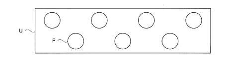
- the distance calculation unit 12 relates to a characteristic configuration of the present invention, and will be described in more detail.
- a phantom unit U as shown in FIG. 2 is used.
- the phantom unit U has a shape in which a cylindrical phantom F extends in a vertical direction from the surface of the base portion from the base portion of the rectangular parallelepiped.
- the phantom unit U has a plurality of phantoms F, and the mutual positional relationship between the outer diameter of each phantom F and the central axis C of each phantom F is known.
- the central axis C of each phantom F extends in the vertical direction.
- FIG. 3 shows the phantom unit U when the phantom unit U is looked down from above.
- the phantom unit U four phantoms F are arranged in the first row, and three phantoms F are arranged in the second row.
- a cylindrical phantom F is used.
- the projected image of the phantom F in the FPD 4 is symmetric.
- the center of the phantom F in the case of a cylindrical shape, the central axis.
- the luminance distribution of the phantom F can be acquired more accurately.
- noise is superimposed on the phantom image reflected in the obtained image. This noise is a hindrance when knowing the luminance distribution of the phantom F. If the phantom images are integrated to generate the profile described in FIG.
- the cylindrical phantom F has a shape suitable for making the phantom F longer.
- ⁇ Phantom shooting step S1> the phantom imaging step S1 for actually capturing an image of the phantom F and generating an X-ray image in which the luminance distribution inside the phantom is reflected will be described.
- an X-ray image P obtained by imaging the phantom unit U is analyzed as shown in FIG.
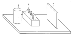
- FIG. 4 shows a state in which the phantom unit U is placed between the X-ray source 3 and the FPD 4.
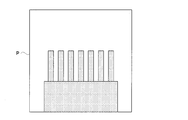
- FIG. 5 is an X-ray image P showing the imaging result of the phantom unit U.
- the projections of the phantom F are reflected without overlapping each other.
- FIG. 6 is an enlarged view of a part of the X-ray image P.
- the phantom image reflected in the X-ray image P is dark at the center, and gradually becomes lighter toward the periphery.
- the reason why the phantom image is reflected in this way is that the width of the phantom F differs depending on the X-ray path. X-rays incident on the central part of the phantom F pass through the thick part of the phantom F and go to the FPD 4, and thus are largely absorbed by the phantom F.
- the X-rays incident on the left and right ends of the phantom F pass through the thin part of the phantom F and go to the FPD 4, so that the phantom F is not so much absorbed.
- Such a difference in the partial X-ray absorption amount of the phantom F appears as a shading of the phantom image.
- a gradation is generated such that the luminance decreases toward the center of the phantom.
- a material that appropriately absorbs X-rays is selected so that this gradation appears.
- the lower side of FIG. 6 shows the relationship between the position on the image in the phantom image and the pixel density as a profile.
- the luminance distribution (profile) has a mountain-like shape as a whole, and the central axis C is likely to be located on the top of this mountain. However, this luminance distribution contains many noise components. In the figure, the noise component is expressed by drawing a short vertical line on the profile.
- a known function that is symmetrical to the luminance distribution may be applied.
- the luminance distribution shown on the lower side of FIG. 6 is based on a projection image of a cylindrical phantom, and therefore should be symmetrical. For example, if a quadratic function approximated to the luminance distribution is obtained by the method of least squares, the central axis C should be located at the maximum point of the quadratic function.
- the lower luminance distribution in FIG. 6 does not necessarily have a quadratic function shape.
- the position of the central axis C may be searched using a function that more faithfully represents the shape of the luminance distribution than the quadratic function.
- the present invention is configured to predict the profile of FIG. 6 by simulation. If a profile is predicted by simulation and an approximate expression is obtained as a result, the positional relationship between the profile and the central axis C can be accurately obtained.
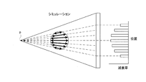
- FIG. 7 shows that it is possible to know how much the X-rays passing through the phantom F are attenuated by simulation.
- X-rays generated from the focal point p which is an X-ray generation point of the X-ray source 3, pass through the phantom F while spreading radially and enter the X-ray detection surface of the FPD 4.
- the X-ray projected on the position where the FPD 4 is located connects the position on the FPD 4 and the focal point p. It ’s a path. It can be known by geometrical calculation where the path of the phantom F passes and the width of the phantom F at that time. This is because the outer diameter of the phantom F is set to a certain dimension. If the width of the phantom F is known, the attenuation coefficient of the X-ray corresponding to the width can be calculated using the absorption coefficient determined by the material of the phantom F. Therefore, the position of the FPD 4 and the X-ray attenuation rate can be associated with each other.
- the left side of FIG. 8 displays the relationship between the position of the FPD 4 described in FIG. 7 and the X-ray attenuation rate.
- the attenuation rate of X-rays represents the shading on the X-ray image obtained by photographing the phantom F. That is, based on the relationship between the position of the FPD 4 and the attenuation factor of the X-ray, as shown on the right side of FIG. 8, the luminance distribution (profile) inside the phantom F in which the position on the X-ray image and the pixel density are related. Can be obtained. That is, on the left side of FIG.
- the attenuation rate is obtained only for the seven points on the FPD 4, but more positions for obtaining the attenuation rate in the FPD 4 can be determined.
- This alone only provides a set of points on which the position and attenuation rate in the FPD 4 are plotted, but by performing a complementary process that compensates between the points, a continuous function as shown on the right side of FIG. 8 is obtained.
- a luminance distribution (profile) inside the phantom F can be obtained. This luminance distribution is obtained not by actual measurement but by simulation. This luminance distribution is the true identity of the approximate expression that faithfully reproduces the lower luminance distribution in FIG.
- the luminance distribution simulation step S2 determines how much X-rays are absorbed by the phantom F when the X-rays are passed through the phantom F placed between the X-ray source 3 and the FPD 4.
- the luminance distribution is simulated by calculating each part of the phantom F.
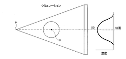
- the luminance distribution of the phantom image is calculated based on the principle as described above. Since this luminance distribution simulation is repeatedly executed, this situation will be described. If the positional relationship between the X-ray source 3 and the phantoms F and FPD4 is determined, it is possible to accurately know where the central axis C of the phantom F is on the FPD4 as shown in FIG. FIG. 9 shows a luminance distribution calculated when the central axis of the phantom F is projected onto the position X0 of the FPD4.
- FIG. 10 shows the luminance distribution calculated when the central axis of the phantom F is projected onto the position X1 of the FPD4. Also in this case, since the positional relationship with the X-ray source 3 and the phantoms F and FPD4 is determined, it is possible to accurately know where the central axis C of the phantom F is on the FPD4 by geometric calculation.
- the luminance distributions for the projection positions X-2, X-1, X0, X1, X2, X3, and X4 of the central axis C of different phantoms F are obtained. Simulated.
- the luminance distributions calculated at this time are very similar to each other, but it is not true if they are completely the same. If the projection position of the central axis C of the phantom F changes, the position of the phantom F with respect to the X-ray source 3 and the FPD 4 changes. This is because the X-ray path passing through the phantom F changes accordingly.
- the luminance distribution for the position X0 is a simulation luminance distribution, and is referred to as a luminance distribution (X0). Such a method of expressing the luminance distribution is the same for other positions. For the sake of explanation, it is assumed that the positions X-2, X-1, X0, X1, X2, X3, and X4 of the FPD 4 are separated by 10 pixels on the X-ray image. The simulation is repeated while moving the phantom F in the y direction so that the position of the central axis C of the phantom image on the FPD 4 moves in the y direction.
- the projection position of the center of the phantom F on the X-ray image is calculated by calculating where the projection position of the center of the phantom F corresponds to the luminance distribution inside the phantom obtained by actual imaging.
- the actual measurement phantom center calculation step S3 will be described.
- the phantom F is placed between the X-ray source 3 and the FPD 4 as shown in FIG. 4 and the phantom F is photographed, the X-ray image P as described with reference to FIG. 5 is obtained. Based on this X-ray image P, it is possible to obtain the luminance distribution inside the phantom F according to the actual measurement described on the lower side of FIG. This luminance distribution should originally represent the same luminance distribution inside the phantom F related to the simulation.
- the luminance distribution inside the phantom F related to the actual measurement includes a noise component, and it is difficult to accurately determine the center. However, it should be possible to accurately overlay the luminance distribution related to the simulation. This is because the two luminance distributions are essentially the same shape although they differ depending on whether they contain a noise component.
- the exact distance between the X-ray source 3 and the FPD 4 when the phantom F is actually measured is unknown. Further, it is difficult to place the phantom F strictly at the ideal position. Therefore, when the simulation is performed, the positional relationship between the X-ray source 3, the phantom F, and the FPD 4 at the time of actual measurement cannot be completely reproduced. Because of such circumstances, the luminance distribution related to the simulation is a slightly enlarged or reduced version of the luminance distribution related to the actual measurement. However, the X-ray source 3, the phantom F, and the FPD 4 at the time of actual measurement are almost in ideal positions, and the two luminance distributions are very similar.
- the actual method for calculating the projection position of the center of the phantom F on the X-ray image will be described.
- the phantom F is actually measured, it is not known where the central axis C of the phantom F is projected on the FPD 4. Therefore, according to the present invention, a plurality of luminance distributions with different projection positions of the central axis C are prepared in the luminance distribution simulation step S2. Assume that the actually measured luminance distribution can be accurately superimposed on the luminance distribution (X-1) obtained by simulation as shown in FIG. In this case, the central axis C of the actually measured phantom image F is projected at the position X-1 on the FPD 4. Such a situation is the same for the luminance distribution in other simulations.
- the position at which the central axis C of the actually measured phantom image F is projected onto the FPD 4 is positions X-2, X-1, X0, X1, X2, and the like on the FPD 4 as shown in FIG. It does not always coincide with any of X3 and X4. Therefore, according to the present invention, even if the position where the central axis C of the actually measured phantom image F is projected onto the FPD 4 is between the position X-1 and the position X0 as shown in FIG. It has the structure which can tell.
- the luminance distribution (X0) is subtracted from the actual luminance distribution to generate a luminance distribution related to the difference.
- the result obtained by integrating the luminance distribution related to the difference by absolute value conversion is referred to as a residual amount ⁇ 0.
- the residual amount ⁇ 0 is an index indicating the degree of coincidence between the two luminance distributions. The smaller the residual amount ⁇ 0 is, the more the both luminance distributions match.
- the calculation of the residual amount is also performed for the other luminance distributions X1, X2, X3, X4,... And the luminance distributions X-1, X-2,.
- FIG. 15 is a graph showing the relationship between positions X1, X2, X3, X4,... And positions X-1, X-2,.
- the residual amount of the luminance distribution (X0) is relatively small.
- the residual amount of the luminance distribution (X1), luminance distribution (X2), luminance distribution (X3), luminance distribution (X4),... Increases as the distance from the luminance distribution X0 increases.
- the residual amounts of the luminance distribution (X-1), luminance distribution (X-2),... Increase as the distance from the luminance distribution (X0) increases.
- each of the positions X-2, X-1, X0, X1, X2, X3, and X4 is 10 pixels apart on the X-ray image
- the central axis of the phantom image related to the actual measurement is on the X-ray image.
- the position is moved by 3 pixels to the left of the position X0.
- the central axis of the phantom F in the actually measured luminance distribution is at a position obtained by moving the central axis C of the simulated luminance distribution X0 to the left by 3 pixels.
- the actual measurement phantom center calculation step S3 repeatedly calculates the difference (residual) between the luminance distributions related to the simulation while changing the luminance distribution related to the simulation with respect to the luminance distribution related to the actual photographing.
- a profile that associates the projection position of the center of the phantom F with the difference corresponding to the position is generated, and the position on the X-ray image that minimizes the difference is obtained based on the profile, thereby obtaining the position of the phantom F on the X-ray image.
- the center projection position is calculated.
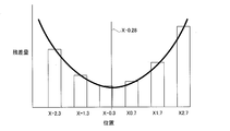
- the upper side of FIG. 16 shows that the luminance distribution X ( ⁇ 0.3) is generated by the same operation as in the luminance distribution simulation step S2. Further, the lower side of FIG. 16 shows the luminance distribution X ( ⁇ 2.3), luminance distribution X ( ⁇ 1.3), luminance distribution X ( ⁇ 0.3), luminance distribution X (0.7) by the same operation. , Luminance distribution X (1.7), and luminance distribution X (2.7) are generated. Such calculation of the luminance distribution can be realized by changing the position of the phantom F with respect to the X-ray tube 3 and the FPD 4 on the simulation.
- FIG. 17 shows the remaining positions corresponding to the positions ⁇ 2.3, ⁇ 1.3, ⁇ 0.3, 0.7, 1.7, and 2.7 generated by the simulation of the new luminance distribution described in FIG. It is a graph showing the relationship with the difference amount.
- the residual amounts for the positions X0.7, X1.7, X2.7,... Increase as the distance from the position X-0.3 increases. Further, the residual amounts for the positions X-1.3, X-2.3,... Increase as the distance from the position X-0.3 increases.
- the central axis of the phantom F in the actually measured luminance distribution is at a position where the central axis C of the simulated luminance distribution X-0.3 is moved to the right by 0.2 pixels.
- the luminance distribution is generated at a position where the position X0 is shifted by 10 pixels in the simulation.
- the luminance distribution X0 is shifted by one pixel or less, and the luminance distribution (X1), luminance Distribution (X2),..., Luminance distribution (X-1), luminance distribution (X-2),... are generated.
- the luminance distribution according to the simulation can be matched with the actual luminance distribution with an accuracy of less than one pixel.
- the projection position of the central axis of the phantom F in the X-ray image P can be accurately known.
- the luminance distribution related to the simulation is changed to the luminance distribution related to the actual measurement because the positional relationship between the X-ray source 3, the phantom F, and the FPD 4 at the actual measurement cannot be completely reproduced during the simulation. It's slightly different. This discrepancy in luminance distribution hinders accurate knowledge of the projection position of the central axis of the phantom F in the X-ray image P.
- a configuration is adopted in which the luminance distribution relating to the simulation is redefined.
- the difference in luminance distribution appears as a difference in the spread width of the distribution. That is, when the distance from the X-ray source 3 to the FPD 4 is different between the simulation and the actual measurement, the magnification of the projection image of the phantom F in the FPD 4 is shifted.
- the example of FIG. 18 explains such a situation.
- the luminance distribution related to the simulation is slightly smaller than the luminance distribution related to the actual measurement.
- the center in the actually measured luminance distribution (that is, the projection position of the central axis C of the phantom F on the X-ray image P) can be obtained by the method described with reference to FIGS. You can ask.
- the brightness distribution according to the simulation is redefined using the calculated center position in the actually measured brightness distribution.
- the center in the temporarily measured luminance distribution is obtained by the method described with reference to FIGS.
- each of the luminance distributions having different magnifications derived from the first luminance distribution is referred to as a “candidate”.
- 11 and 17 are overlapped in a state where the center of the actually measured luminance distribution obtained by the method described with reference to FIGS. 11 to 17 is matched with the center of the candidate 1 (that is, the position of the central axis C of the phantom). Then, it can be seen that the width of candidate 1 does not match the width of the actually measured luminance distribution.
- Such a match evaluation can be understood by calculating a mean square error between the luminance distributions. If such a match evaluation is also performed on other candidates, it is possible to find the one whose width most closely matches the width of the actually measured luminance distribution. In FIG. 18, candidate 2 is most suitable for the width of the actually measured luminance distribution.
- the phantom F is placed between the X-ray source 3 and the FPD 4 so as to reproduce the positional relationship between the X-ray sources 3, FPD4 and phantom F in each simulation described with reference to FIGS.
- FIG. 21 illustrates the principle of obtaining the distance between the X-ray source 3 and the FPD 4.
- the distance from the X-ray source 3 to the FPD 4 is Di, and the distance from the X-ray source 3 to the central axis C1 of the phantom F1 related to the first imaging is D1.
- the distance between the two phantoms F1 related to the first shooting is w.
- the distance between the phantoms F is the same w in the second shooting.
- ⁇ d be the distance between the phantom F1 related to the first shooting and the phantom F2 related to the second shooting.
- the distances D1 and Di are unknown, and the distances w and ⁇ d are known.
- the distance between the central axes C of the two phantoms F1 related to the first shooting projected on the FPD4 is R1
- the distance between the central axes C of the two phantoms F2 related to the second shooting projected onto the FPD4 is R1.
- the distances R1 and R2 are known values that can be obtained very accurately by the method described with reference to FIGS.
- the distance calculation unit 12 calculates the distance between the X-ray source 3 and the FPD 4 based on the principle described with reference to FIGS.
- the X-ray imaging apparatus 1 is provided with an ideal distance D0 between the X-ray source 3 and the FPD 4.
- the positional relationship between them is adjusted so that the distance between the X-ray source 3 and the FPD 4 is the distance D0. Therefore, the distance between the X-ray source 3 and the FPD 4 is approximately D0.
- the distance between the two is actually measured Di, which is slightly different from the ideal distance D0.
- the size of the subject image projected on the FPD 4 changes when the subject is photographed. In other words, if the distance between the X-ray source 3 and the FPD 4 is larger than the ideal distance D0, the subject image of the FPD 4 appears larger than the expected size. If the distance between the X-ray source 3 and the FPD 4 is smaller than the ideal distance D0, the subject image of the FPD 4 appears smaller than the expected size.
- the distance calculation unit 12 sends the measured value of the distance Di to the tomographic image generation unit 15.
- the tomographic image generation unit 15 changes parameters necessary for generating a tomographic image based on the actually measured value of the distance Di. As a result, even if the distance between the X-ray source 3 and the FPD 4 remains out of the ideal, the same tomographic image generated when the distance is as ideal can be generated. By such an operation, the tomographic image generation unit 15 can make the dimensions of the subject tomographic image on the tomographic image as actual. With this operation, the calibration operation using the phantom F is completed.
- Each X-ray image PM is sent to the tomographic image generation unit 15.
- Each X-ray image PM is taken in a state where the distance between the X-ray source 3 and the FPD 4 is a distance Di different from the ideal distance D0, and the subject image on the X-ray image PM is a distance.
- the image is enlarged or reduced from the ideal by the amount of deviation.
- the tomographic image generation unit 15 generates a tomographic image when there is no enlargement or reduction of the image on the X-ray image PM due to a shift in distance.
- the tomographic image generation unit 15 at this time can generate the tomographic image D by using the filter-corrected back projection method (FBP method).
- FBP method filter-corrected back projection method
- the tomographic image of the subject reflected in the tomographic image D generated in this way has an accurate size. This is because the tomographic image D at this time is equivalent to the image taken with the distance between the X-ray source 3 and the FPD 4 set to the ideal distance D0.
- the dimensional deviation of the subject image on the X-ray image PM appears as it is as the dimensional deviation of the tomographic image on the tomographic image D.
- the dimensional deviation of the subject image on the X-ray image PM is corrected in advance before the tomographic image D is generated, the dimensional deviation does not occur in the tomographic image D as well.
- the apparatus includes a storage unit 20 that stores all information related to control of the apparatus, and a display unit 21 that displays a tomographic image D.
- the main control unit 25 includes a CPU and the like, and realizes the above-described control units 6 and 8 and the image processing units 11, 12, 13, 14, and 15 by executing various programs. Each unit may be realized by being divided into control devices in charge of these.
- the positional relationship between the X-ray source 3 and the FPD 4 can be calculated more accurately.
- a spherical phantom F is photographed, and the center of the phantom F is calculated from the outline of a circular projection image appearing in the X-ray image.
- the center of the phantom F is calculated by a very small outline portion of the projected image of the phantom F.
- the center of the phantom F can be known more accurately than before by calculating using the entire phantom. Can do.
- the center of the phantom F can be calculated from the circular outline by analyzing the image.
- the luminance distribution of the phantom F is obtained by simulation. If the projected position of the center of the phantom F is known in the simulated brightness distribution, the projected position of the center of the phantom F in the measured brightness distribution can be easily and accurately known.
- the difference is generated by changing the position of the luminance distribution related to the simulation by the width of one pixel on the X-ray image.
- the difference obtained at this time is compared, and the center of the phantom F corresponding to the luminance distribution with the smallest difference indicates the projected position of the center of the phantom F on the X-ray image.
- the above-described configuration is further stepped down to generate a profile in which the projection position at the center of the phantom F in the luminance distribution related to the simulation is associated with the difference corresponding to the position. If this profile is used, the projection position of the center of the phantom F on the X-ray image can be calculated with an accuracy of less than one pixel.
- the present invention is not limited to the above-described configuration, and can be modified as follows.
- the phantom F has a cylindrical shape, but the present invention is not limited to this configuration.
- the present invention can also be realized by using the phantom F as a rotating body other than a cylindrical shape. If the phantom F is a rotating body, the center of the phantom F becomes the central axis of the rotating body, and the luminance distribution of the phantom F is symmetric. In this way, it becomes easy to accurately calculate the projection position of the central axis on the X-ray image P.
- the present invention is configured to calculate the projection position of the central axis in the X-ray image P by searching for the center of the actually measured luminance distribution described in the lower part of FIG.
- the measured luminance distribution is uneven in shape on the right and left sides of the central axis, it becomes difficult to find the center of the luminance distribution. This is because the middle of the luminance distribution becomes unclear. If the phantom F is a rotating body, such a situation does not occur.
- the X-ray imaging apparatus 1 is configured to capture the tomographic image D, but the present invention is not limited to such a configuration.
- the present invention can also be applied to an apparatus that captures only a fluoroscopic image.
- FIG. 23 shows the configuration of this modification.
- the measured value of the distance between the X-ray source 3 and the FPD 4 calculated by the distance calculation unit 12 is transmitted to the magnification calculation unit 13.
- the magnification calculation unit 13 is configured to calculate an image enlargement magnification necessary for canceling a change in the size of the subject image caused by the distance between the X-ray source 3 and the FPD 4 being not ideal.
- the magnification calculator 13 calculates a deviation amount indicating how much the distance between the X-ray source 3 and the FPD 4 is deviated from the ideal value of the distance based on the actually measured value of the distance Di.
- the magnification calculator 13 calculates the enlargement ratio of the X-ray image based on the amount of deviation.
- the magnification calculation unit 13 projects the X-ray to a large extent on the X-ray image by projecting the FPD 4 larger than expected. It is calculated whether the size of the subject image on the X-ray image obtained when the distance between the source 3 and the FPD 4 is an ideal value. Further, when the actually measured value of the distance is smaller than the ideal value, the magnification calculation unit 13 projects the X-ray to a small extent on the subject image reflected on the X-ray image by being projected on the FPD 4 smaller than expected. Whether the size of the subject image on the X-ray image obtained when the distance between the source 3 and the FPD 4 is ideal is calculated. The result of such calculation is the magnification. The magnification calculator 13 is sent to the image corrector 14. With this operation, the calibration operation using the phantom F is completed.
- the X-ray image PM is sent to the image correction unit 14.
- the image correction unit 14 performs enlargement or reduction image processing on the X-ray image PM based on the magnification obtained by the calibration operation.
- Each X-ray image PM before correction is taken in a state where the distance between the X-ray source 3 and the FPD 4 is different from the ideal, and the subject image on the X-ray image PM is ideal by the amount of the deviation of the distance.
- the image is magnified or reduced.
- the image correction unit 14 corrects the variation in the size of the subject image on the X-ray image PM due to the distance between the X-ray source 3 and the FPD 4 being not ideal, and Of the subject image to the dimensions.
- the present invention is suitable for the industrial field.
Landscapes
- Physics & Mathematics (AREA)
- Health & Medical Sciences (AREA)
- Life Sciences & Earth Sciences (AREA)
- Chemical & Material Sciences (AREA)
- Analytical Chemistry (AREA)
- Biochemistry (AREA)
- General Health & Medical Sciences (AREA)
- General Physics & Mathematics (AREA)
- Immunology (AREA)
- Pathology (AREA)
- Apparatus For Radiation Diagnosis (AREA)
- Analysing Materials By The Use Of Radiation (AREA)
Abstract
画像上のファントム像の中心の位置を正確に求める。円柱形のファントムFの投影像の輝度分布のプロファイルをシミュレーションで求めたプロファイルにフィッティングすることでファントムの中心を求める。投影像の輪郭から中心を算出する従来方法と比較して、ファントム投影像の全体から中心を求めるので、統計ノイズなどの影響を受けにくく正確にファントムの中心を知ることができる。このファントム中心の値は投影像の正確な倍率計算などに利用する。
Description
本発明は、検査対象に放射線を照射して、断層画像を生成することができる放射線撮影装置を構成する各部材の位置関係を測定する測定方法および、当該方法を適用した放射線撮影装置に関する。
工場などには、検査対象に放射線を照射して、断層画像を生成する放射線撮影装置が配備されている。このような装置は、図24に示すように支持台52と、放射線を照射する放射線源53と、検査対象である試料を載置する回転テーブル55と、放射線を検出する検出器54とを備えている。ここで、放射線源53は、水平方向に放射線を照射するように設置されている。放射線源53から照射された放射線は、回転テーブル55に置かれている試料を透過して検出器54に入射する。検出器54は、放射線を検出することで画像を生成する。
本発明に係る装置では、回転テーブル55が放射線源53および検出器54に対して回転する構成となっている。放射線を照射し、回転テーブル55を回転させながら画像を連写すれば、さまざまな投影方向についての画像が得られる。本発明に係る装置は、これら連写された画像に基づいて断層画像を生成する。この断層画像は、連写画像を再構成したCT(Computed Tomography)画像となっている。断層画像は、試料の断面構造を明らかにするものとなっている。
この様な放射線撮影装置は、単に試料内部の形状を知るだけではなく、試料内部の構造物の寸法を測定するのにも用いられる。試料内部の構造物の寸法を正確に測定しようとすると、放射線源53と検出器54との間の距離が正確に分かっていなければならない。図25はこの理由を説明している。放射線源53は、放射状に広がる放射線を検出器54に向けて照射する。この放射線は、次第に広がりながら回転テーブル55上の試料を透過し、検出器54に投影される。図25上側に示すように、放射線源53と検出器54との間の距離が近いと、試料の投影は検出器54において小さく写り込む。連写画像の各々に写り込んでいる試料が小さいと、連写画像の各々によって再構成された断層画像には、試料の断層像が小さく写り込む。
逆に、図25下側に示すように、放射線源53と検出器54との間の距離が遠いと、試料の投影は検出器54において大きく写り込む。連写画像の各々に写り込んでいる試料が大きいと、連写画像の各々によって再構成された断層画像には、試料の断層像が大きく写り込む。つまり、放射線源53と検出器54との間の距離によって断層画像上における試料の断層像の寸法が変動してしまうのである。
断層画像に写り込む断層像の寸法を正確に知る工夫としては、放射線源53と検出器54との間の距離を所定の距離に定めるという方法がある。この様にすると、放射線源53と検出器54との間の距離は一定の既知な値になるので、断層画像上の断層像が拡大したり縮小したりしなくなる。
ところが、放射線源53と検出器54との距離を厳密に設定値とするのは相当難しい。実際の放射線源53と検出器54との距離は、設定値(理想の距離)よりもわずかに異なっている。このときの差異はほんのわずかなものではある。しかし、この差異が影響して、断層画像上の断層像が理想の大きさから拡大または縮小してしまう。
そこで、放射線源53と検出器54との距離を厳密に設定値にするのではなく、放射線源53と検出器54との距離を測定して、断層画像上の断層像が理想の大きさからどの程度拡大または縮小してしまっているかを知るという構成が考え出されている。これが分かれば、断層像が理想の大きさになるように断層画像に対して縮小または拡大する画像処理を施すことができる。この様な画像処理により、断層像の寸法が正確な断層画像を得ることができる。
放射線源53と検出器54との距離を測定するには、回転テーブル55上に置かれたファントムを撮影する方法が用いられる。検出器54においてファントムが写り込む位置を実測することにより、幾何学的な計算により放射線源53と検出器54との距離を知ることができる。
図26左側は、球体のファントムを撮影したときに得られる透視画像を示している。球体のファントムは、黒い円形の像として透視画像のどこかに写り込む。透視画像上における黒い円形のファントム像の中心点の位置を正確に求めないと、放射線源53と検出器54との距離を正確に知ることができない。このとき必要とされる位置の精度は、中心点が透視画像を構成する画素のうちのどれに位置するかが分かる程度では足りない。放射線源53と検出器54との距離を正確に知るには、例えば、画素幅の1/100の精度で中心点の位置を言い当てるぐらいの精度が必要となる。
画像上のファントム像の位置を正確に知ることは、断層画像上の断層像の寸法の正確性を担保するのに重要である。ファントム像の位置を正確に求めようとする様々な工夫は従来からなされている。図26右側は、ファントム像の輪郭を用いて中心を求めている。球体ファントム像の輪郭は円形となり、この円の中心がファントム像の中心点を意味している(例えば引用文献1参照)。
しかしながら、従来のファントム位置の検出方法には次のような問題点がある。
すなわち、従来の方法では、ファントム像の位置を算出する精度に限界がある。
すなわち、従来の方法では、ファントム像の位置を算出する精度に限界がある。
画像上のファントム像の輪郭は、放射線の散乱線成分、統計ノイズ等の影響により画像上で滲んでしまっている。また、放射線源53が特定の一点から放射線を発生させていないことによっても輪郭の滲みが発生する。輪郭だけでファントム像の中心点を求めるような従来構成では、この様な画像上の輪郭の滲みがファントム像の位置を正確に算出するときの妨げとなっている。
本発明は、この様な事情に鑑みてなされたものであって、その目的は、放射線撮影装置を構成する各部材の位置関係を検出する方法であって、画像上のファントム像の位置を正確に知ることができる方法を提供して、画像上の断層像の寸法をより正確にすることを目的とする。
本発明は上述の課題を解決するために次のような構成をとる。
すなわち、本発明に係る測定方法は、放射線を照射する放射線源と、放射線を検出する検出器とを備えた放射線撮影装置における放射線源と検出器との位置関係の測定方法において、ファントムを実際に撮影してファントム内部の輝度分布が写り込んだ放射線画像を生成するファントム撮影ステップと、ファントム内部の輝度分布をシミュレートする輝度分布シミュレーションステップと、シミュレーションに係る輝度分布におけるファントムの中心の投影位置が実際の撮影に係るファントム内部の輝度分布上のどこに対応するのかを算出することにより、放射線画像上におけるファントムの中心の投影位置を算出する実測ファントム中心算出ステップと、算出された放射線画像上のファントムの中心の投影位置に基づいて放射線源と検出器との位置関係を算出する位置関係算出ステップを備えることを特徴とするものである。
すなわち、本発明に係る測定方法は、放射線を照射する放射線源と、放射線を検出する検出器とを備えた放射線撮影装置における放射線源と検出器との位置関係の測定方法において、ファントムを実際に撮影してファントム内部の輝度分布が写り込んだ放射線画像を生成するファントム撮影ステップと、ファントム内部の輝度分布をシミュレートする輝度分布シミュレーションステップと、シミュレーションに係る輝度分布におけるファントムの中心の投影位置が実際の撮影に係るファントム内部の輝度分布上のどこに対応するのかを算出することにより、放射線画像上におけるファントムの中心の投影位置を算出する実測ファントム中心算出ステップと、算出された放射線画像上のファントムの中心の投影位置に基づいて放射線源と検出器との位置関係を算出する位置関係算出ステップを備えることを特徴とするものである。
[作用・効果]本発明によれば、放射線源と検出器との位置関係をより正確に算出することができる。従来構成は、例えば球形のファントムを撮影し、放射線画像に現れる円形の投影像の輪郭からファントムの中心を算出するというものである。従来構成では、ファントムの中心は、ファントムの投影像のごく一部の輪郭部で算出されてしまう。本発明によれば、ファントム内部の輝度分布からファントムの中心を算出するようにするようにしているので、ファントム全体を用いて算出をすることにより、従来よりも正確にファントムの中心を知ることができる。
球形のファントムを撮影する従来例では、円形の投影像が現れることが分かっているから画像の解析により円形の輪郭からファントムの中心を算出することができる。それに対して本発明では、ファントムの投影像の中の輝度分布全体を利用してファントムの中心位置を求めるために、シミュレーションによりファントムの輝度分布を求めるようにしている。シミュレーション上の輝度分布において、ファントムの中心の投影位置を知っておけば、実測に係る輝度分布におけるファントムの中心の投影位置を容易かつ正確に知ることができる。
球形のファントムを撮影する従来例では、円形の投影像が現れることが分かっているから画像の解析により円形の輪郭からファントムの中心を算出することができる。それに対して本発明では、ファントムの投影像の中の輝度分布全体を利用してファントムの中心位置を求めるために、シミュレーションによりファントムの輝度分布を求めるようにしている。シミュレーション上の輝度分布において、ファントムの中心の投影位置を知っておけば、実測に係る輝度分布におけるファントムの中心の投影位置を容易かつ正確に知ることができる。
また、上述の測定方法において、輝度分布シミュレーションステップは、放射線源と、検出器との間に載置されたファントムに放射線を通過させた際、放射線がファントムにどの程度吸収されるかをファントムの各部で算出することにより輝度分布をシミュレートすればより望ましい。
[作用・効果]上述の構成は、本発明をより具体的に示したものとなっている。放射線がファントムにどの程度吸収されるかをファントムの各部で算出すれば、輝度分布を確実にシミュレートすることができる。
また、上述の測定方法において、ファントム撮影ステップが複数のファントムが同時に写り込んでいる放射線画像を生成すればより望ましい。
[作用・効果]上述の構成は、本発明をより具体的に示したものとなっている。複数のファントムに基づいて放射線源と検出器との位置関係を算出するようにすれば、位置関係をより確実に算出することができる。
また、上述の測定方法において、ファントムは回転体となっていればより望ましい。
[作用・効果]上述の構成は、本発明をより具体的に示したものとなっている。ファントムが回転体であれば、ファントムの中心は、回転体の中心軸となり、ファントムの輝度分布が左右対称になる。この様にすると、正確な中心軸の算出が可能となる。
また、上述の測定方法において、実測ファントム中心算出ステップが実際の撮影に係る輝度分布に対してシミュレーションに係る輝度分布の位置を変えながら互いの輝度分布の差分を繰り返し算出し、シミュレーションに係る輝度分布におけるファントムの中心の投影位置と当該位置に対応する差分を関連づけたプロファイルを生成し、プロファイルに基づいて差分が最低となる放射線画像上の位置を求めることにより放射線画像上のファントムの中心の投影位置を算出すればより望ましい。
[作用・効果]上述の構成は、本発明をより具体的に示したものとなっている。上述の構成によれば、放射線画像上のファントムの中心の投影位置をより正確に算出することができる。シミュレーションに係る輝度分布の位置を放射線画像上の画素1ピクセルの幅ずつ変えて差分を生成したとする。このとき得られた差分を比較して、差分が最も小さかった輝度分布に対応するファントムの中心が放射線画像上のファントムの中心の投影位置を示していることになる。上述の構成は更に踏み込んで、シミュレーションに係る輝度分布におけるファントムの中心の投影位置と当該位置に対応する差分を関連づけたプロファイルを生成する。このプロファイルを用いれば画素1ピクセル未満の精度で放射線画像上のファントムの中心の投影位置を算出することができる。
本発明によれば、放射線源と検出器との位置関係をより正確に算出することができる。本発明によれば、円柱形のファントムFの投影像の輝度分布のプロファイルをシミュレーションで求めたプロファイルにフィッティングすることでファントムの中心を求める。投影像の輪郭から中心を算出する従来方法と比較して、ファントム投影像の全体から中心を求めるので、統計ノイズなどの影響を受けにくく正確にファントムの中心を知ることができる。このファントム中心の値は投影像の正確な倍率計算などに利用する。
これより図面を参照しながら、本発明に係る放射線撮影装置について説明する。本発明に係る放射線撮影装置は、断層画像を撮影することができる。X線は、本発明の放射線に相当する。FPDは、フラットパネルディテクタの略である。
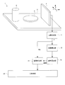
図1は、本発明に係るX線撮影装置の全体像を表している。図1に示すように本発明に係るX線撮影装置1は、装置を構成する各部品を載置する支持台2を備え、支持台2には、検査対象に向けてX線を照射するX線源3と、検査対象を透過したX線を検出するFPD4と、X線源3とFPD4とに挟まれる位置に置かれた円盤形状の回転テーブル5を有している。回転テーブル5には、検査対象を載置することができる。X線源3から照射されたX線は回転テーブル5の上空を通過してFPD4に到達する。X線源3はX線管を主体としてX線を発生するものであり、本発明の放射線源に相当する。また、FPDは2次元的な面状に並んだ画素ごとにX線を検出するものであり、本発明の検出器に相当する。
回転テーブル5は、X線源3およびFPD4に対して回転することができる。回転機構7は、回転テーブル5を回転させる機構であり、例えばモータを有している。回転制御部8は、回転機構7の回転速度や回転ステップ量を制御する構成である。回転機構7は、X線源3からFPD4に向かうx方向と直交するz方向(鉛直方向)に伸びた軸を回転軸として回転テーブル5を回転させることにより回転テーブル5上の検査対象を回転させる。
この回転テーブル5は、検査物を載置する台となっている。回転テーブル5を回転させると、回転テーブル5は、自転するように回転し、これに追従して回転テーブル5上の検査物も回転する。X線源3から照射されたX線は、回転テーブル5上の検査物を透過してFPD4に到達する。したがって、本発明の装置は、回転テーブル5上の検査物のX線撮影を行うことができる。また、回転テーブル5を回転させながら画像の撮影を行えば、検査物について撮影角度の異なる画像を連続的に得ることができる。
X線源制御部6は、X線源3の管電圧や管電流を制御する構成である。
画像生成部11は、FPD4が出力するX線の検出信号に基づいて画像を生成する構成である。画像生成部11は、X線源3よりX線が照射され、FPD4が出力したX線の検出信号を受信し画像を生成する。回転テーブル5が一回転する間に180回の撮影が行われるとすれば、画像生成部11は検査物に対してX線照射方向の異なる180枚の画像を生成することになる。
断層画像生成部15は、画像生成部11が生成した一連の画像を再構成することにより断層画像Dを生成する。断層画像生成部15が断層画像Dを生成するには、回転テーブル5が1回転する間に撮影された一連の画像に対して再構成処理を行う必要がある。
距離算出部12は、X線源3とFPD4(FPD4におけるX線が入射する検出面)との距離を算出する目的で設けられている。この距離算出部12は、本発明の特徴的な構成に関しているので、より詳しく説明する。
X線源3とFPD4との距離を算出するには、図2に示すようなファントムユニットUが用いられる。ファントムユニットUは、直方体の基部から円柱形のファントムFが基部の面から垂直方向に伸びた形状をしている。ファントムユニットUは、複数のファントムFを有しており、各ファントムFの外径と各ファントムFの中心軸Cの相互位置関係は既知である。支持台2または回転テーブル5に載置したときには各ファントムFの中心軸Cはいずれも鉛直方向に伸びている。
図3は、ファントムユニットUを上から見下ろしたときのファントムユニットUを表している。ファントムユニットUには1行目に4つのファントムFが配列しており、2行目に3つのファントムFが配列している。
本実施例は円柱形状のファントムFを採用している。ファントムFが円柱形状であると、FPD4におけるファントムFの投影像が左右対称となる。この様にすると、ファントムFの中心(円柱形状の場合は中心軸)を発見しやすいという利点がある。また、ファントムFを長くすれば、ファントムFの輝度分布をより正確に取得することができる。ファントムFを撮影すると、得られる画像に写り込んでいるファントム像にはノイズが重畳する。このノイズは、ファントムFの輝度分布を知るときの妨げになる。ファントム像を積算して図6に説明するプロファイルを生成すれば、ノイズ同士が相殺される。ファントムFが長いと画像に写り込むファントム像も長くなりそれだけ積算されるデータが増える。したがって、ファントムFを長くすればノイズの影響を確実に除去してファントムFの輝度分布を知ることができる。円柱形状のファントムFは、ファントムFを長くするのに適した形状となっている。
<ファントム撮影ステップS1>
続いて、ファントムFを実際に撮影してファントム内部の輝度分布が写り込んだX線画像を生成するファントム撮影ステップS1について説明する。X線源3とFPD4との距離を算出するには、図4に示すようにファントムユニットUを撮影して得られるX線画像Pの解析がなされる。図4は、ファントムユニットUがX線源3とFPD4と間に載置されている様子を示している。
続いて、ファントムFを実際に撮影してファントム内部の輝度分布が写り込んだX線画像を生成するファントム撮影ステップS1について説明する。X線源3とFPD4との距離を算出するには、図4に示すようにファントムユニットUを撮影して得られるX線画像Pの解析がなされる。図4は、ファントムユニットUがX線源3とFPD4と間に載置されている様子を示している。
図5は、ファントムユニットUの撮影結果を示すX線画像Pである。X線画像Pには、ファントムFの投影が互いに重なることなく写り込んでいる。X線源3とFPD4との距離を算出するには、各ファントムFの中心軸CがX線画像P上のどこに写り込んでいるかを正確に知る必要がある。
図6は、X線画像Pの一部を拡大したものである。X線画像Pに写り込むファントム像は、中心部が濃く、そこから周辺部に向かうに従って次第に薄く写り込んでいる。ファントム像がこの様に写り込む理由は、ファントムFの幅がX線のパスによって異なるからである。ファントムFの中心部に入射したX線は、ファントムFの厚い部分を通過してFPD4に向かうのでファントムFで多く吸収される。また、ファントムFの左右両端部に入射したX線は、ファントムFの薄い部分を通過してFPD4に向かうのでファントムFであまり吸収されない。このようなファントムFの部分的なX線吸収量の違いがファントム像の濃淡となって現れる。X線画像Pに写り込むファントム像には、ファントムの中心部に向かって輝度が低くなるようなグラデーションが発生している。ファントムFを構成する素材としては、このグラデーションが現れるように適度にX線を吸収するものが選択される。
図6の下側は、ファントム像における画像上の位置と画素濃度との関係をプロファイルとして示したものである。輝度分布(プロファイル)は、全体としては山のような形状となっており、中心軸Cはこの山の頂上に位置しそうである。しかし、この輝度分布には、多くのノイズ成分が含まれている。図の上では、ノイズ成分はプロファイル上に短い縦線を描くことで表現している。
この様な輝度分布からファントムFの中心軸Cの位置を算出するには、輝度分布に左右対称となっている既知の関数を当てはめればよい。図6の下側に示す輝度分布は円柱形状のファントムの投影像を基にしているので左右対称になっているはずである。例えば輝度分布に近似した二次関数を最小二乗法により求めれば、中心軸Cは、二次関数の極大点に位置するはずである。
図6の下側の輝度分布は、二次関数の形状になるとは限らない。より正確に中心軸Cの位置を求めるには、二次関数よりももっと輝度分布の形状を忠実に表した関数を用いて中心軸Cの位置を探すようにすればよい。
そこで、本発明は、シミュレーションにより図6のプロファイルを予想しておく構成となっている。シミュレーションによりプロファイルを予測してその結果で近似式を得るようにすれば、プロファイルと中心軸Cとの位置関係を正確に求めることができる。
<輝度分布シミュレーションステップS2>
ファントム内部の輝度分布をシミュレートする輝度分布シミュレーションステップS2について説明する。図7は、シミュレーションによりファントムFを通過したX線がどの程度減衰するか知ることができることを表している。X線源3のX線の発生点である焦点pから生じたX線は放射状に広がりながらファントムFを透過し、FPD4におけるX線の検出面に入射する。シミュレーションを実行する際に予めX線源3,ファントムF,FPD4の位置関係を定めておけば、X線がFPD4のある位置に投影されたX線は、FPD4上の位置と焦点pとを結ぶパスを通ってきたことになる。このパスがファントムFのどこを通過し、そのときのファントムFの幅がどの程度だったかは、幾何学的計算で知ることができる。ファントムFの外径は、ある寸法に定められているからである。ファントムFの幅が分かれば、ファントムFの材質によって定まっている吸収係数を利用して、その幅に対応するX線の減衰率を計算することができる。したがって、FPD4の位置とX線の減衰率とを関連づけて対応させることができる。
ファントム内部の輝度分布をシミュレートする輝度分布シミュレーションステップS2について説明する。図7は、シミュレーションによりファントムFを通過したX線がどの程度減衰するか知ることができることを表している。X線源3のX線の発生点である焦点pから生じたX線は放射状に広がりながらファントムFを透過し、FPD4におけるX線の検出面に入射する。シミュレーションを実行する際に予めX線源3,ファントムF,FPD4の位置関係を定めておけば、X線がFPD4のある位置に投影されたX線は、FPD4上の位置と焦点pとを結ぶパスを通ってきたことになる。このパスがファントムFのどこを通過し、そのときのファントムFの幅がどの程度だったかは、幾何学的計算で知ることができる。ファントムFの外径は、ある寸法に定められているからである。ファントムFの幅が分かれば、ファントムFの材質によって定まっている吸収係数を利用して、その幅に対応するX線の減衰率を計算することができる。したがって、FPD4の位置とX線の減衰率とを関連づけて対応させることができる。
図8左側は、図7で説明したFPD4の位置とX線の減衰率との関連性を表示している。X線の減衰率は、ファントムFを撮影して得られるX線画像上の濃淡を表している。すなわち、FPD4の位置とX線の減衰率との関連性に基づいて、図8右側に示すように、X線画像上の位置と画素の濃度とが関連したファントムF内部の輝度分布(プロファイル)を得ることができる。すなわち、図8左側では、FPD4上の7点についてしか減衰率を求めていないが、FPD4における減衰率を求める位置をより多く定めることができる。これだけではFPD4における位置と減衰率とがプロットされた点の集合が得られるに過ぎないが、各点の間を補う補完処理を施すことにより、図8右側に示すような連続関数となっているファントムF内部の輝度分布(プロファイル)を得ることができる。この輝度分布は実測ではなく、シミュレーションにより求められるものとなっている。この輝度分布こそが図6の下側の輝度分布を忠実に再現した近似式の正体である。このように、輝度分布シミュレーションステップS2は、X線源3と、FPD4との間に載置されたファントムFにX線を通過させた際、X線がファントムFにどの程度吸収されるかをファントムFの各部で算出することにより輝度分布をシミュレートする。
輝度分布シミュレーションステップS2では、上述のような原理でファントム像の輝度分布を算出するわけである。この輝度分布のシミュレーションは繰り返し実行されるのでこの事情について説明する。X線源3,ファントムF,FPD4との位置関係を定めれば、図9に示すようファントムFの中心軸CがFPD4上のどこに来るかを幾何学的な計算により正確に知ることができる。図9においては、ファントムFの中心軸がFPD4のX0の位置に投影される場合において算出される輝度分布を表している。
輝度分布シミュレーションステップS2では、X線源3,FPD4に対するファントムFの位置を変えながら上述のシミュレーションを何度も繰り返す。図10は、ファントムFの中心軸がFPD4のX1の位置に投影される場合において算出される輝度分布を表している。この場合もX線源3,ファントムF,FPD4との位置関係が定まっているから、ファントムFの中心軸CがFPD4上のどこに来るかを幾何学的な計算により正確に知ることができる。
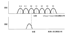
この様にして輝度分布シミュレーションステップS2では、図11に示すように、異なるファントムFの中心軸Cの投影位置X-2,X-1,X0,X1,X2,X3,X4についての輝度分布がシミュレートされる。このとき算出される輝度分布は互いによく似ているが、完全に同じかというとそうでもない。ファントムFの中心軸Cの投影位置が変われば、X線源3,FPD4に対するファントムFの位置が変わる。これに伴い、ファントムFを通過するX線のパスが変わってくるからである。位置X0についての輝度分布は、シミュレーションの輝度分布であり、輝度分布(X0)と呼ぶことにする。この様な輝度分布の表現方法は、他の位置についても同様である。説明上、FPD4の位置X-2,X-1,X0,X1,X2,X3,X4のそれぞれは、X線画像上では10ピクセルずつ離れているものとする。シミュレーションの繰り返しは、FPD4上におけるファントム像の中心軸Cの位置がy方向に移動するように、ファントムFをy方向に移動させながら行われる。
<実測ファントム中心算出ステップS3>
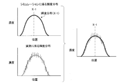
続いて、ファントムFの中心の投影位置が実際の撮影で得られたファントム内部の輝度分布上のどこに対応するのかを算出することにより、X線画像上におけるファントムFの中心の投影位置を算出する実測ファントム中心算出ステップS3について説明する。図4に示したようにファントムFをX線源3とFPD4との間に載置して、ファントムFを撮影すると、図5で説明したようなX線画像Pが得られる。このX線画像Pに基づいて図6の下側で説明した実測に係るファントムF内部の輝度分布を得ることができる。この輝度分布は、本来はシミュレーションに係るファントムF内部の輝度分布と同じものを表しているはずである。
続いて、ファントムFの中心の投影位置が実際の撮影で得られたファントム内部の輝度分布上のどこに対応するのかを算出することにより、X線画像上におけるファントムFの中心の投影位置を算出する実測ファントム中心算出ステップS3について説明する。図4に示したようにファントムFをX線源3とFPD4との間に載置して、ファントムFを撮影すると、図5で説明したようなX線画像Pが得られる。このX線画像Pに基づいて図6の下側で説明した実測に係るファントムF内部の輝度分布を得ることができる。この輝度分布は、本来はシミュレーションに係るファントムF内部の輝度分布と同じものを表しているはずである。
実測に係るファントムF内部の輝度分布は、ノイズ成分を含んでおり、どこが中心なのか正確に判断することが難しい。しかし、これにシミュレーションに係る輝度分布を正確に重ね合わせることはできるはずである。2つの輝度分布は、ノイズ成分を含んでいるかで違うものの本来的には同じ形状をしているはずだからである。
なお、ファントムFを実測したときのX線源3およびFPD4の厳密な距離は未知である。また、ファントムFを厳密に理想の位置に置くことは難しい。したがって、シミュレーションを行う際には、実測時のX線源3,ファントムF,FPD4の位置関係を完全に再現することができない。このような事情があるので、シミュレーションに係る輝度分布は、実測に係る輝度分布をわずかに拡大または縮小したものとなってしまう。とはいえ、実測時のX線源3,ファントムF,およびFPD4はほぼ理想通りの位置にあり、2つの輝度分布は、酷似したものとなっていることには変わりはない。
X線画像上におけるファントムFの中心の投影位置を算出する方法の実際について説明する。ファントムFを実測したとき、ファントムFの中心軸CがFPD4のどこに投影されているか分からない。そこで本発明によれば、輝度分布シミュレーションステップS2において中心軸Cの投影位置が異なる輝度分布を複数用意するようにしている。仮に、実測の輝度分布が図12に示すようにシミュレーションで求めた輝度分布(X-1)に正確に重ね合わせることができたとする。この場合、実測のファントム像Fの中心軸CはFPD4上の位置X-1に投影されることになる。この様な事情は他のシミュレーション上の輝度分布についても同じである。
つまり、シミュレーションで求めた図11に描かれている複数の輝度分布のうちのどれかが実測の輝度分布に類似していれば、実測のファントム像Fの中心軸CがFPD4上のどこに投影されたかを言い当てることができる。
とはいうものの、実際は、実測のファントム像Fの中心軸CがFPD4に投影される位置は、図13に示すようにFPD4の上の位置X-2,X-1,X0,X1,X2,X3,X4のどれかに完全に一致するとは限らない。そこで、本発明によれば、実測のファントム像Fの中心軸CがFPD4に投影される位置が図13に示すように位置X-1と位置X0との間にあったとしても正確にFPD4上の位置を言い当てることができる構成を有している。
この構成について説明する。実測ファントム中心算出ステップS3では、まず図14に示すように、実測の輝度分布から輝度分布(X0)が減算され差分に係る輝度分布を生成する。この差分に係る輝度分布を絶対値変換して積分したものを残差量α0と呼ぶことにする。残差量α0は、両輝度分布の一致度を示す指標である。残差量α0が小さいほど両輝度分布は一致していたことになる。
このような残差量の算出は、他の輝度分布X1,X2,X3,X4,…および輝度分布X-1,X-2,…についても行われる。こうして、残差量α0,α1,α2,α3,α4,…および残差量α-1,α-2,…が算出される。
図15は、位置X1,X2,X3,X4,…および位置X-1,X-2,…これらに対応する残差量との関係をグラフにしたものである。輝度分布(X0)の残差量は比較的小さい。輝度分布(X1),輝度分布(X2),輝度分布(X3),輝度分布(X4),…の残差量は、輝度分布X0から遠ざかるほど大きくなる。同様に、輝度分布(X-1),輝度分布(X-2),…の残差量は輝度分布(X0)から遠ざかるほど大きくなる。
輝度分布を横軸、残差量を縦軸にして互いの関連性を示す関数を考える。この関数は、輝度分布X0を中心に左右対称の形状をしているはずである。しかし実際に、この様な関数を最小二乗法により求めてみると、関数の対称線は、輝度分布X0からわずかにずれる。このズレは、実測の輝度分布の中心がX0の位置になかったことに起因している。図15では、対称線は、X-0.3の位置に現れている。位置X-2,X-1,X0,X1,X2,X3,X4のそれぞれは、X線画像上では10ピクセルずつ離れていたからことからすると、実測に係るファントム像の中心軸は、X線画像上において、位置X0よりも左に3ピクセルだけ移動したところにあることになる。
このようなマッチング処理により、実測の輝度分布におけるファントムFの中心軸は、シミュレーションの輝度分布X0の中心軸Cを左に3ピクセルだけ移動させた位置にあることが分かる。このように、実測ファントム中心算出ステップS3は、実際の撮影に係る輝度分布に対してシミュレーションに係る輝度分布を変えながら互いの輝度分布の差分(残差)を繰り返し算出し、シミュレーションに係る輝度分布におけるファントムFの中心の投影位置と当該位置に対応する差分を関連づけたプロファイルを生成し、プロファイルに基づいて差分が最低となるX線画像上の位置を求めることによりX線画像上のファントムFの中心の投影位置を算出する構成となっている。
同様のマッチング処理を繰り返すことにより実測の輝度分布におけるファントムFの中心軸のより正確な位置を知ることもできる。
図16上側は、輝度分布シミュレーションステップS2と同様な操作によって、輝度分布X(-0.3)を生成しているところを示している。また、図16下側は、同様な操作によって輝度分布X(-2.3),輝度分布X(-1.3),輝度分布X(-0.3),輝度分布X(0.7),輝度分布X(1.7),輝度分布X(2.7)が生成されたところを示している。この様な輝度分布の算出は、シミュレーション上でX線管3およびFPD4に対するファントムFの位置を変更することで実現できる。
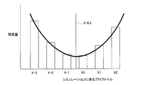
図17は、図16で説明した新たな輝度分布のシミュレーションによって生成された位置-2.3,-1.3,-0.3,0.7,1.7,2.7に対応する残差量との関係をグラフにしたものである。位置X0.7,X1.7,X2.7,…についての残差量は、位置X-0.3から遠ざかるほど大きくなる。また、位置X-1.3,X-2.3,…についての残差量は位置X-0.3から遠ざかるほど大きくなる。
輝度分布を横軸、残差量を縦軸にして互いの関連性を示す関数を考える。この関数は輝度分布X-0.3を中心に左右対称の形状をしているはずである。しかし実際に、この様な関数を最小二乗法により求めてみると、関数の対称線は、輝度分布X-0.3からわずかにずれる。図16では、対称線は、X-0.28の位置に現れている。これは、輝度分布X-0.3を右に0.2ピクセルだけ移動させると、より実測の輝度分布に一致することを表している。
このようなマッチング処理により、実測の輝度分布におけるファントムFの中心軸は、シミュレーションの輝度分布X-0.3の中心軸Cを右に0.2ピクセルだけ移動させた位置にあることが分かる。
なお、図11では、シミュレーションにおいて位置X0を10ピクセルずつシフトした位置について輝度分布を生成していたが、実際は輝度分布X0を1ピクセルまたはそれより小さい間隔でシフトして輝度分布(X1),輝度分布(X2),…および輝度分布(X-1),輝度分布(X-2),…が生成される。この様な構成とすることにより、1ピクセルに満たない精度でシミュレーションに係る輝度分布を実際の輝度分布にマッチングさせることができる。
この様にして、本発明によれば、X線画像PにおけるファントムFの中心軸の投影位置を正確に知ることができる。
なお、上述のように、シミュレーション時に実測時のX線源3,ファントムF,FPD4の位置関係を完全に再現することができないことに起因して、シミュレーションに係る輝度分布が実測に係る輝度分布にわずかに食い違ってしまっている。この輝度分布の食い違いは、X線画像PにおけるファントムFの中心軸の投影位置を正確に知る上で妨げとなる。本発明ではこの問題を解決する目的で、シミュレーションに係る輝度分布の再定義を行うような構成を採用している。
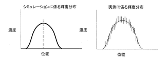
この方法について説明する。輝度分布の食い違いは、分布の広がり幅の違いとして現れる。すなわち、X線源3からFPD4までの距離がシミュレーションと実測とで互いに異なることにより、FPD4におけるファントムFの投影像の拡大率がずれてしまったのである。図18の例では、この様な事情を説明している。シミュレーションに係る輝度分布は、実測に係る輝度分布よりも一回り小さくなっている。
このように輝度分布に多少の食い違いがあっても、図11ないし図17で説明した方法により、実測の輝度分布における中心(すなわちX線画像P上におけるファントムFの中心軸Cの投影位置)は求めることはできる。本発明によれば、この算出された実測の輝度分布における中心位置を利用して、シミュレーションに係る輝度分布の再定義を行う。まず、図11ないし図17で説明した方法で暫定の実測の輝度分布における中心を求めておく。
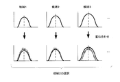
そして、図18に示すように、シミュレーションに係る輝度分布を異なる倍率で拡大または縮小したものを複数用意する。こうして生成された輝度分布の中には、図19の左側で説明した最初の輝度分布よりも実測の輝度分布に近いものが含まれているはずである。現時点では、どれが実測に近いものなのか判断できないので、最初の輝度分布から派生した拡大倍率の異なる各輝度分布のそれぞれを「候補」と呼ぶことにする。
図11ないし図17で説明した方法で求めた実測の輝度分布における中心と候補1の中心(すなわちファントムの中心軸Cの位置)とを一致させた状態で両者を重ね合わせてみる。すると、候補1の幅は、実測の輝度分布の幅に合っていないことが分かる。この様な合致の評価は、輝度分布同士の間で平均二乗誤差を算出することで分かる。この様な合致の評価を他の候補に対しても行えば、最も幅が実測の輝度分布の幅に合っているものを探し出すことができる。図18においては、候補2が最も実測の輝度分布の幅に合っている。シミュレーションに係る輝度分布をこの候補2に置き換えて、輝度分布の再定義をした後、図11ないし図17で説明した方法により、実測の輝度分布における中心を再び求めれば、より正確なX線画像P上のファントムFの中心軸Cの投影位置を算出することができる。
<位置関係算出ステップS4>
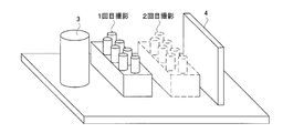
続いて、算出されたX線画像P上のファントムFの中心の投影位置に基づいてX線源3とFPD4との位置関係を算出する位置関係算出ステップS4について説明する。X線源3とFPD4との距離を求めるには、少なくとも2つのファントムが同時に写り込んでいるX線画像Pの撮影を2回行う必要がある。図20の実線で示すファントムユニットUは、1回目の撮影を説明しており、破線で示すファントムユニットUは、2回目の撮影を説明している。X線源3とFPD4との間にファントムユニットUを載置して1回目の撮影を終えた後、ファントムユニットUをFPD4側に移動させてもう一度撮影が実行される。このときの移動距離は既知である。
続いて、算出されたX線画像P上のファントムFの中心の投影位置に基づいてX線源3とFPD4との位置関係を算出する位置関係算出ステップS4について説明する。X線源3とFPD4との距離を求めるには、少なくとも2つのファントムが同時に写り込んでいるX線画像Pの撮影を2回行う必要がある。図20の実線で示すファントムユニットUは、1回目の撮影を説明しており、破線で示すファントムユニットUは、2回目の撮影を説明している。X線源3とFPD4との間にファントムユニットUを載置して1回目の撮影を終えた後、ファントムユニットUをFPD4側に移動させてもう一度撮影が実行される。このときの移動距離は既知である。
ファントムFは、図7,図9で説明した各シミュレーションにおけるX線源3,FPD4,およびファントムFの位置関係を再現するようにX線源3とFPD4との間に置かれる。
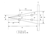
図21は、X線源3とFPD4との距離を求める原理を説明している。X線源3からFPD4までの距離をDiとし、X線源3から一回目の撮影に係るファントムF1の中心軸C1までの距離をD1とする。一回目の撮影に係る2つのファントムF1の距離をwとする。ファントムF同士の距離は、二回目の撮影でも同じwとなる。一回目の撮影に係るファントムF1と二回目の撮影に係るファントムF2との距離をΔdとする。距離D1,Diは未知であり、距離w,Δdは既知である。
なお、FPD4に投影された一回目の撮影に係る2つのファントムF1の中心軸C間の距離をR1とし、FPD4に投影された二回目の撮影に係る2つのファントムF2の中心軸C間の距離をR2とする。この距離R1,R2は図6から図19で説明した方法により極めて正確に求めることができる既知の値である。
これらパラメータには、次のような関係がある。
D1 : Di = w : R1
D1+Δd : Di = w : R2
これらの関連性により次のような連立方程式が得られる。
D1・R1=wDi
R2(D1+Δd)=wDi
この連立方程式を解けば、距離D1,Diを求めることができる。
D1 : Di = w : R1
D1+Δd : Di = w : R2
これらの関連性により次のような連立方程式が得られる。
D1・R1=wDi
R2(D1+Δd)=wDi
この連立方程式を解けば、距離D1,Diを求めることができる。
距離算出部12は、このような図6から図21で説明した原理に基づいてX線源3とFPD4との距離を算出する。
X線撮影装置1には、X線源3とFPD4の理想の距離D0が設けられている。X線撮影装置1をメンテナンスする際に、X線源3およびFPD4の距離がこの距離D0となるように両者の位置関係が調整される。したがって、X線源3とFPD4との間の距離はほぼD0となる。しかし、両者間の距離を完全にD0とするのは難しい。両者間の距離は、実測されたDiとなっており、理想の距離D0とはわずかに異なる。
X線源3とFPD4との距離が変動すると、被写体を撮影するときにFPD4に投影される被写体像の大きさが変化する。すなわち、X線源3とFPD4との距離が理想の距離D0より大きいと、FPD4の被写体像は、想定上の大きさよりも大きく写り込む。X線源3とFPD4との距離が理想の距離D0より小さいと、FPD4の被写体像は、想定上の大きさよりも小さく写り込む。
距離算出部12は、距離Diの実測値を断層画像生成部15に送出する。断層画像生成部15は、距離Diの実測値に基づいて、断層画像を生成するときに必要なパラメータを変更する。これにより、X線源3とFPD4との間の距離が理想から外れたままであっても、距離が理想通りとなっているときに生成される断層画像と同じものが生成できるようになる。断層画像生成部15はこの様な動作により、断層画像上の被検体断層像の寸法を実際の通りにすることができる。この動作により、ファントムFを用いた校正動作は終了となる。
<断層画像の撮影>
続いて、校正動作完了後のX線撮影装置1を用いた断層画像Dの撮影について説明する。被写体Mの断層画像Dを撮影するには、図22に示すように回転テーブル5に被写体Mがセットされる。操作者が入力部22を通じて断層画像Dの撮影の指示を行うと、回転テーブル5が回転されながらX線画像PMの連写が実行される。
続いて、校正動作完了後のX線撮影装置1を用いた断層画像Dの撮影について説明する。被写体Mの断層画像Dを撮影するには、図22に示すように回転テーブル5に被写体Mがセットされる。操作者が入力部22を通じて断層画像Dの撮影の指示を行うと、回転テーブル5が回転されながらX線画像PMの連写が実行される。
各X線画像PMは、断層画像生成部15に送出される。各X線画像PMは、X線源3とFPD4との距離が理想の距離D0とは異なる距離Diとなっている状態で撮影されたものであり、X線画像PM上の被写体像は、距離のズレの分だけ理想より拡大または縮小されて写り込んでいる。断層画像生成部15は、ファントムFを用いた校正の結果、距離のズレに起因するX線画像PM上の像の拡大または縮小がなかったときの断層画像を生成する。このときの断層画像生成部15は、フィルタ補正逆投影法(FBP法)を用いて断層画像Dを生成することができる。
この様に生成された断層画像Dに写り込む被写体の断層像は、寸法が正確なものとなっている。このときの断層画像Dは、X線源3とFPD4との距離を理想の距離D0にして撮影したものと等価となっているからである。補正なしのX線画像PMに基づいて断層画像Dを生成すると、X線画像PM上における被写体像の寸法の狂いがそのまま断層画像D上における断層像の寸法の狂いとして現れてしまう。本発明によれば、断層画像Dを生成する前に予めX線画像PM上における被写体像の寸法の狂いが正されているので、断層画像D上においても断層像に寸法の狂いが生じない。
<その他の構成>
本発明に係る装置は、装置の制御に関する情報の一切を記憶する記憶部20と、断層画像Dを表示する表示部21とを備えている。主制御部25は、CPUなどから構成され、各種のプログラムを実行することにより上述の各制御部6,8および各画像処理部11,12,13,14,15を実現する。各部は、これらを担当する制御装置に分割されて実現されていてもよい。
本発明に係る装置は、装置の制御に関する情報の一切を記憶する記憶部20と、断層画像Dを表示する表示部21とを備えている。主制御部25は、CPUなどから構成され、各種のプログラムを実行することにより上述の各制御部6,8および各画像処理部11,12,13,14,15を実現する。各部は、これらを担当する制御装置に分割されて実現されていてもよい。
以上のように、本発明によれば、X線源3とFPD4との位置関係をより正確に算出することができる。従来構成は、例えば球形のファントムFを撮影し、X線画像に現れる円形の投影像の輪郭からファントムFの中心を算出するというものである。従来構成では、ファントムFの中心は、ファントムFの投影像のごく一部の輪郭部で算出されてしまう。本発明によれば、ファントム内部の輝度分布からファントムFの中心を算出するようにするようにしているので、ファントム全体を用いて算出をすることにより従来よりも正確にファントムFの中心を知ることができる。
球形のファントムFを撮影する従来例では、円形の投影像が現れることが分かっているから画像の解析により円形の輪郭からファントムFの中心を算出することができる。それに対して本発明では、ファントムFの投影像の中の輝度分布全体を利用してファントムの中心位置を求めるために、シミュレーションによりファントムFの輝度分布を求めるようにしている。シミュレーション上の輝度分布において、ファントムFの中心の投影位置を知っておけば、実測に係る輝度分布におけるファントムFの中心の投影位置を容易かつ正確に知ることができる。
シミュレーションに係る輝度分布の位置をX線画像上の画素1ピクセルの幅ずつ変えて差分を生成したとする。このとき得られた差分を比較して、差分が最も小さかった輝度分布に対応するファントムFの中心がX線画像上のファントムFの中心の投影位置を示していることになる。上述の構成は更に踏み込んで、シミュレーションに係る輝度分布におけるファントムFの中心の投影位置と当該位置に対応する差分を関連づけたプロファイルを生成する。このプロファイルを用いれば画素1ピクセル未満の精度でX線画像上のファントムFの中心の投影位置を算出することができる。
本発明は、上述の構成に限られず下記のように変形実施することもできる。
(1)図2によれば、ファントムFは、円柱形状であったが、本発明はこの構成に限られない。ファントムFを円柱形状以外の回転体としても本発明を実現できる。ファントムFが回転体であれば、ファントムFの中心は、回転体の中心軸となり、ファントムFの輝度分布が左右対称になる。この様にすると、X線画像P上の中心軸の投影位置を正確に算出しやすくなる。本発明は、図6下側で説明した実測の輝度分布の中心を探すことでX線画像Pにおける中心軸の投影位置を算出する構成である。実測の輝度分布に中心軸の右側と左側とで形状に偏りがあると、輝度分布の中心を探し出すことが難しくなってしまう。輝度分布の真ん中が判然としなくなるからである。ファントムFが回転体となっていれば、この様な事態が生じない。
(2)図1によれば、X線撮影装置1は断層画像Dを撮影できる構成となっていたが、本発明はこの様な構成に限られない。本発明は、透視画像のみを撮影する装置についても適用できる。図23はこの変形例の構成を示している。
本変形例の実際について説明する。距離算出部12が算出したX線源3とFPD4間の距離の実測値は、倍率算出部13に送信される。倍率算出部13は、X線源3とFPD4との距離が理想通りとなっていないことに起因する被写体像の大きさの変動をキャンセルするのに必要な画像の拡大倍率を算出する構成である。倍率算出部13は、距離Diの実測値に基づいてX線源3とFPD4間の距離が距離の理想値からどの程度ずれているかを示すズレ量を算出する。倍率算出部13は、このズレ量に基づいてX線画像の拡大率を算出する。
すなわち、倍率算出部13は、距離の実測値が理想値よりも大きい場合、FPD4に想定よりも大きく投影されることによりX線画像上で大きく写り込んだ被写体像をどの程度縮小すればX線源3とFPD4との距離が理想値であったときに得られるX線画像上の被写体像の大きさになるかを算出する。また、倍率算出部13は、距離の実測値が理想値よりも小さい場合、FPD4に想定よりも小さく投影されることによりX線画像上で小さく写り込んだ被写体像をどの程度拡大すればX線源3とFPD4との距離が理想通りであったときに得られるX線画像上の被写体像の大きさになるかを算出する。このような算出の結果が倍率である。倍率算出部13は、画像補正部14に送出される。この動作により、ファントムFを用いた校正動作は終了となる。
X線画像PMは、画像補正部14に送出される。画像補正部14は、校正動作で求められた倍率に基づいてX線画像PMに拡大または縮小の画像処理を施す。補正前の各X線画像PMは、X線源3とFPD4との距離が理想とは異なる状態で撮影されたものであり、X線画像PM上の被写体像は、距離のズレの分だけ理想より拡大または縮小されて写り込んでいる。画像補正部14は、このX線源3とFPD4との間の距離が理想通りとなっていないことによるX線画像PM上の被写体像の大きさの変動を補正して、X線画像PM上の被写体像を寸法通りにする。
以上のように、本発明は、工業分野に適している。
3 X線源(放射線源)
4 FPD(検出器)
S1 ファントム撮影ステップ
S2 輝度分布シミュレーションステップ
S3 ファントム中心シミュレーションステップ
S4 実測ファントム中心算出ステップ
S5 位置関係算出ステップ
4 FPD(検出器)
S1 ファントム撮影ステップ
S2 輝度分布シミュレーションステップ
S3 ファントム中心シミュレーションステップ
S4 実測ファントム中心算出ステップ
S5 位置関係算出ステップ
Claims (6)
- 放射線を照射する放射線源と、放射線を検出する検出器とを備えた放射線撮影装置における前記放射線源と前記検出器との位置関係の測定方法において、
ファントムを実際に撮影してファントム内部の輝度分布が写り込んだ放射線画像を生成するファントム撮影ステップと、
ファントム内部の輝度分布をシミュレートする輝度分布シミュレーションステップと、
シミュレーションに係る輝度分布における前記ファントムの中心の投影位置が実際の撮影に係るファントム内部の輝度分布上のどこに対応するのかを算出することにより、前記放射線画像上における前記ファントムの中心の投影位置を算出する実測ファントム中心算出ステップと、
算出された放射線画像上の前記ファントムの中心の投影位置に基づいて前記放射線源と前記検出器との位置関係を算出する位置関係算出ステップを備えることを特徴とする測定方法。 - 請求項1に記載の測定方法において、
前記輝度分布シミュレーションステップは、前記放射線源と、前記検出器との間に載置された前記ファントムに放射線を通過させた際、放射線が前記ファントムにどの程度吸収されるかを前記ファントムの各部で算出することにより輝度分布をシミュレートすることを特徴とする測定方法。 - 請求項1に記載の測定方法において、
前記ファントム撮影ステップが複数の前記ファントムが同時に写り込んでいる放射線画像を生成することを特徴とする測定方法。 - 請求項1に記載の測定方法において、
前記ファントムは回転体となっていることを特徴とする測定方法。 - 請求項1に記載の測定方法において、
前記実測ファントム中心算出ステップが実際の撮影に係る輝度分布に対してシミュレーションに係る輝度分布の位置を変えながら互いの輝度分布の差分を繰り返し算出し、シミュレーションに係る輝度分布におけるファントムの中心の投影位置と当該投影位置に対応する差分を関連づけたプロファイルを生成し、前記プロファイルに基づいて差分が最低となる放射線画像上の位置を求めることにより放射線画像上の前記ファントムの中心の投影位置を算出することを特徴とする測定方法。 - 請求項1に記載の測定方法により前記放射線源と前記検出器との位置関係が算出されていることを特徴とする放射線撮影装置。
Applications Claiming Priority (2)
| Application Number | Priority Date | Filing Date | Title |
|---|---|---|---|
| JP2015-106691 | 2015-05-26 | ||
| JP2015106691A JP2018119786A (ja) | 2015-05-26 | 2015-05-26 | 測定方法および放射線撮影装置 |
Publications (1)
| Publication Number | Publication Date |
|---|---|
| WO2016190218A1 true WO2016190218A1 (ja) | 2016-12-01 |
Family
ID=57393193
Family Applications (1)
| Application Number | Title | Priority Date | Filing Date |
|---|---|---|---|
| PCT/JP2016/064896 Ceased WO2016190218A1 (ja) | 2015-05-26 | 2016-05-19 | 測定方法および放射線撮影装置 |
Country Status (2)
| Country | Link |
|---|---|
| JP (1) | JP2018119786A (ja) |
| WO (1) | WO2016190218A1 (ja) |
Families Citing this family (1)
| Publication number | Priority date | Publication date | Assignee | Title |
|---|---|---|---|---|
| JP7239285B2 (ja) * | 2018-08-27 | 2023-03-14 | セメス株式会社 | X線検査装置 |
Citations (7)
| Publication number | Priority date | Publication date | Assignee | Title |
|---|---|---|---|---|
| JPH0747060A (ja) * | 1993-08-03 | 1995-02-21 | Hamamatsu Photonics Kk | 円筒状物体の内径測定方法 |
| JP2753517B2 (ja) * | 1988-06-10 | 1998-05-20 | ジェネラル エレクトリック セージェーエール ソシエテ アノニム | 1つまたは複数の円形偏心ファントムを用いたx線スキャナの較正方法とシステム |
| JP2002131246A (ja) * | 2000-10-25 | 2002-05-09 | Shimadzu Corp | X線撮像装置における撮像倍率の較正方法 |
| JP2009150667A (ja) * | 2007-12-19 | 2009-07-09 | Hitachi-Ge Nuclear Energy Ltd | 検査装置,検査装置のアライメント方法及び校正用ファントムの製作方法 |
| JP2009276142A (ja) * | 2008-05-13 | 2009-11-26 | Hitachi Ltd | 放射線検査システム及び放射線検査の撮像方法 |
| US20100195804A1 (en) * | 2009-02-02 | 2010-08-05 | Arineta Ltd. | Method for calibration of a ct scanner |
| JP2010204060A (ja) * | 2009-03-06 | 2010-09-16 | Hitachi-Ge Nuclear Energy Ltd | X線検査装置及びx線検査装置の検査方法 |
-
2015
- 2015-05-26 JP JP2015106691A patent/JP2018119786A/ja active Pending
-
2016
- 2016-05-19 WO PCT/JP2016/064896 patent/WO2016190218A1/ja not_active Ceased
Patent Citations (7)
| Publication number | Priority date | Publication date | Assignee | Title |
|---|---|---|---|---|
| JP2753517B2 (ja) * | 1988-06-10 | 1998-05-20 | ジェネラル エレクトリック セージェーエール ソシエテ アノニム | 1つまたは複数の円形偏心ファントムを用いたx線スキャナの較正方法とシステム |
| JPH0747060A (ja) * | 1993-08-03 | 1995-02-21 | Hamamatsu Photonics Kk | 円筒状物体の内径測定方法 |
| JP2002131246A (ja) * | 2000-10-25 | 2002-05-09 | Shimadzu Corp | X線撮像装置における撮像倍率の較正方法 |
| JP2009150667A (ja) * | 2007-12-19 | 2009-07-09 | Hitachi-Ge Nuclear Energy Ltd | 検査装置,検査装置のアライメント方法及び校正用ファントムの製作方法 |
| JP2009276142A (ja) * | 2008-05-13 | 2009-11-26 | Hitachi Ltd | 放射線検査システム及び放射線検査の撮像方法 |
| US20100195804A1 (en) * | 2009-02-02 | 2010-08-05 | Arineta Ltd. | Method for calibration of a ct scanner |
| JP2010204060A (ja) * | 2009-03-06 | 2010-09-16 | Hitachi-Ge Nuclear Energy Ltd | X線検査装置及びx線検査装置の検査方法 |
Also Published As
| Publication number | Publication date |
|---|---|
| JP2018119786A (ja) | 2018-08-02 |
Similar Documents
| Publication | Publication Date | Title |
|---|---|---|
| JP6133231B2 (ja) | X線エネルギースペクトル測定方法およびx線エネルギースペクトル測定装置およびx線ct装置 | |
| KR100667014B1 (ko) | 단층상 및 3차원 화상작성방법 | |
| JP6735667B2 (ja) | コンピュータ断層撮影の較正装置および方法 | |
| CN103648392B (zh) | X射线ct装置、计算装置以及x射线ct装置的维护方法 | |
| JP6711410B2 (ja) | 放射線断層撮影装置の撮像倍率校正方法 | |
| US20170205360A1 (en) | X-ray imaging system allowing the correction of the scatter radiation and precise detection of the distance between the source and the detector | |
| Ferrucci et al. | Measurement of the X-ray computed tomography instrument geometry by minimization of reprojection errors—Implementation on simulated data | |
| US20170365077A1 (en) | Device and method for image reconstruction at different x-ray energies, and device and method for x-ray three-dimensional measurement | |
| JP2010523950A (ja) | 透過する放射線を用いて計測対象の三次元画像を生成するための方法および計測装置 | |
| JP4959223B2 (ja) | 断層撮影装置 | |
| JP2018509600A (ja) | 線形検出器アレイ用のギャップ分解能 | |
| CN1861001A (zh) | 一种适用于三维ct扫描系统投影坐标原点的标定方法 | |
| JP7670380B2 (ja) | コンピュータ断層撮影撮像のための散乱補正 | |
| JP2020515830A (ja) | 対象物のデジタルモデルに基づく対象物に対するx線ユニットの姿勢の算出 | |
| CN112535490B (zh) | X射线ct装置及其校正方法和装置、测定方法和装置 | |
| US20140003573A1 (en) | X-Ray CT System for Measuring Three Dimensional Shapes and Measuring Method of Three Dimensional Shapes by X-Ray CT System | |
| JP7542327B2 (ja) | 検査装置 | |
| CN108333197A (zh) | 偏置扫描模式下工业ct系统转台旋转中心标定方法 | |
| KR101680602B1 (ko) | 3차원 내부 영상 복원 시스템, 3차원 내부 영상 복원 장치, 3차원 내부 영상 복원 방법 및 기록 매체 | |
| CN101341395A (zh) | 计算机化层面摄影系统及方法 | |
| WO2015054946A1 (zh) | Ct投影旋转中心的确定方法和装置 | |
| WO2016190218A1 (ja) | 測定方法および放射線撮影装置 | |
| JP2015075336A (ja) | 再構成画像生成装置、形状測定装置、構造物製造システム、再構成画像生成方法及び再構成画像生成プログラム | |
| Sire et al. | X-ray cone beam CT system calibration | |
| JP2004061256A (ja) | コンピュータ断層撮影装置 |
Legal Events
| Date | Code | Title | Description |
|---|---|---|---|
| 121 | Ep: the epo has been informed by wipo that ep was designated in this application |
Ref document number: 16799924 Country of ref document: EP Kind code of ref document: A1 |
|
| NENP | Non-entry into the national phase |
Ref country code: DE |
|
| 122 | Ep: pct application non-entry in european phase |
Ref document number: 16799924 Country of ref document: EP Kind code of ref document: A1 |
|
| NENP | Non-entry into the national phase |
Ref country code: JP |