JP2004266587A - Time-sequential signal encoding apparatus and recording medium - Google Patents
Time-sequential signal encoding apparatus and recording medium Download PDFInfo
- Publication number
- JP2004266587A JP2004266587A JP2003055114A JP2003055114A JP2004266587A JP 2004266587 A JP2004266587 A JP 2004266587A JP 2003055114 A JP2003055114 A JP 2003055114A JP 2003055114 A JP2003055114 A JP 2003055114A JP 2004266587 A JP2004266587 A JP 2004266587A
- Authority
- JP
- Japan
- Prior art keywords
- sample
- sample sequence
- time
- value
- sub
- Prior art date
- Legal status (The legal status is an assumption and is not a legal conclusion. Google has not performed a legal analysis and makes no representation as to the accuracy of the status listed.)
- Granted
Links
Images


Abstract
Description
【0001】
【産業上の利用分野】
本発明は、音楽制作、音響データの素材保管、ロケ素材の中継など音楽制作分野、CD・DVD等のデジタル記録媒体を用いたオーディオ記録再生、遠隔医療における生体信号の解析・診断等の分野において好適なデータの圧縮符号化技術に関する。
【0002】
【従来の技術】
従来より、音響信号の圧縮には様々な手法が用いられている。音響信号を圧縮して符号化する手法として、MP3(MPEG−1/Layer3)、AAC(MPEG−2/Layer3)などが実用化されている。このような圧縮符号化方式により、音響信号を小さいデータとして扱うことが可能となり、データの記録・伝送の効率化に貢献している。
【0003】
最近では、上述のようなMP3、AAC等のロッシー符号化方式だけでなく、完全に復元することが可能なロスレス符号化方式も開発されており、音響素材の管理に用いられている(例えば、特許文献1参照)。
【0004】
【特許文献1】
特表2000−821199号公報
【0005】
【発明が解決しようとする課題】
高精細オーディオを扱う場合は、通常のオーディオ(音楽CD品質:サンプリング周波数44.1kHz、量子化ビット数16ビット)に比べ、サンプリング周波数または量子化ビット数を高く設定してサンプリングしている。音楽編集分野では、さまざまな音をミックスして編集する作業がしばしば行われるが、この際、部分的に通常のオーディオがミックスされる場合があり、この通常のオーディオについては、高精細オーディオに合わせるべく、サンプルの補間、量子化ビット数の引き伸ばし等が行われる。このような補間処理を施された音響信号は、原理的に原音がもつ情報量程度に圧縮を行うことが可能であるが、従来のロスレス符号化方式で符号化を行っても、その程度の圧縮効果が得られない。逆に、そのまま線形予測符号化を中心とした圧縮を行うと、補間された箇所の線形予測誤差が増大して圧縮率が劣化する場合もあり、冗長箇所を圧縮するのとは逆効果にもなり得る。例えば、サンプリング周波数を2倍に拡大したオーディオデータは、理論上は50%以下に圧縮可能なはずであるが、現実には50%を超える圧縮率になってしまう。
【0006】
そこで、このような問題を解決するため、本発明は、デジタル編集途上の高精細オーディオのワークデータを効率的に可逆圧縮することが可能な時系列信号の符号化装置および記録媒体を提供することを課題とする。
【0007】
【課題を解決するための手段】
上記課題を解決するため、本発明では、時系列のサンプル列で構成される時系列信号に対して、前記全てのサンプル列を再現できるように情報量を圧縮する符号化装置として、前記サンプル列に対して、録音により作成された主サンプル列と、主サンプル列を補間処理することにより得られた副サンプル列を分離すると共に、前記副サンプル列中の各副サンプルの値を、近傍の主サンプルの平均値と当該副サンプルの値との差分値に変換するサンプル列再配置手段と、前記主サンプル列、前記変換された副サンプル列それぞれに対して、線形予測誤差を算出し、前記主サンプル列および前記副サンプル列の値をそれぞれ予測誤差値に変換する予測誤差変換手段と、前記予測誤差値に変換された主サンプル列、副サンプル列を可変長で符号化する可変長符号化手段を有する構成としたことを特徴とする。
【0008】
本発明によれば、時系列信号を構成するサンプル列を、録音により得られた主サンプル列と、主サンプル列を補間することにより得られた副サンプル列に再配置し、主サンプル列と副サンプル列それぞれに対して予測符号化し、可変長符号化するようにしたので、デジタル編集途上の高精細オーディオのワークデータを効率的に可逆圧縮することが可能となる。
【0009】
【発明の実施の形態】
以下、本発明の実施形態について図面を参照して詳細に説明する。
(第1の実施形態)
図1は、本発明に係る時系列信号の符号化装置の第1の実施形態を示す構成図である。図1において、10は時系列信号入力手段、20はサンプル列再配置手段、30は下位固定ビット削除手段、40は予測誤差変換手段、50はチャンネル間演算手段、60は極性処理手段、70は可変長符号化手段である。
【0010】
図1において、時系列信号入力手段10はデジタル音響信号等のデジタル化された音響信号を入力する機能を有している。サンプル列再配置手段20は、入力された時系列信号であるサンプル列を録音を基に得られたサンプル列である主サンプル列と主サンプル列を補間することにより得られた副サンプル列とに分離する機能を有している。下位固定ビット削除手段30は、量子化雑音成分である下位の所定数のビットを削除する機能を有している。予測誤差変換手段40は、線形予測誤差の手法を用いて、各サンプルの値を予測誤差値に変換する機能を有する。チャンネル間演算手段50は、複数のチャンネルからなるサンプル列の各チャンネル間の差分演算を行う機能を有する。極性処理手段60は、正負の値を補数表現により表した各サンプルのビット列を、正負の極性を表す1ビットと他のビット列に分ける処理を行う機能を有する。可変長符号化手段70は、各サンプルの値を可変ビット長で符号化する機能を有している。図1に示した装置は、実際には、コンピュータおよびコンピュータにインストールされた専用のソフトウェアプログラムにより実現される。
【0011】
次に、図1に示した時系列信号の符号化装置の処理動作について説明する。本発明では、時系列信号として複数の音響信号をミックスしたワークデータを扱う場合を例にとって説明する。このような音響信号は、上述のように、サンプリング周波数48kHz、量子化ビット数16ビットの通常の音響信号や、サンプリング周波数96kHz、量子化ビット数24ビットの高精細の音響信号が混在している。このようにサンプリング周波数の異なる音響信号を混在させることにより得られる音響信号は、高精細の音響信号にサンプリング周波数を統一させて扱うことになる。この場合、サンプリング周波数48kHzの音響信号は、サンプリング周波数96kHzの音響信号にサンプル数を合わせるべく隣接するサンプルの平均値で間を補間していく。
【0012】
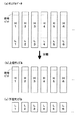
このような音響信号を模式的に示すと図2(a)のようになる。図2(a)において括弧内の数字は、1から昇順に付されたサンプル番号であり、xは、そのサンプルの値を示している。このようなサンプル列である時系列信号が時系列信号入力手段10から入力されると、サンプル列再配置手段20は、奇数番目のサンプルについて、その両隣の偶数番目のサンプルの平均値との差分を演算すると共に、偶数番目のサンプルについて、その両隣の奇数番目のサンプルの平均値との差分を演算する。このときのサンプル列を模式的に示すと、それぞれ図2(b)(c)に示すようになる。なお、図2(b)の例では、演算を行わない偶数番目のサンプルを、図2(c)の例では、奇数番目のサンプルを、それぞれ時間的に過去に移動させた状態で示している。
【0013】
この差分演算の結果、差分値が小さいものが多い方を副サンプル列とし、少ない方を主サンプル列とする。図2の例では、図2(b)の配列の後半分の各値と、
図2(c)の配列の後半分の各値とを比較することになる。例えば、奇数番目のサンプルが補間によって得られたものである場合、図2(b)に示した配列の後半の値が0になる。一方、偶数番目のサンプルが補間によって得られたものである場合、図2(c)に示した配列の後半の値が0に近くなる。例えば、図2(b)に示す配列の後半に0近辺の値が多い場合、偶数番目のサンプルの集合を主サンプル列、奇数番目のサンプルの集合を副サンプル列として分離する。また、サンプル列再配置手段20の処理においては、図2(b)(c)に示したように主サンプルを時間的に過去に移動し、副サンプルを時間的に未来に移動させるようにしても良いが、主サンプルと副サンプルを分離して扱うようにしても良い。例えば、奇数番目が副サンプルの場合には、図2(d)に示すように主サンプルと副サンプルを分離する。本発明においては、本来のサンプルを利用して補間することにより得られたサンプルを含んだサンプル列に対して線形予測を行うことにより、逆にデータ量が増えてしまうことを防ぐために、主サンプル列と副サンプル列を区別している。そのため、主サンプル列と副サンプル列に対して、別々に線形予測を行うことができれば、図2(b)(c)に示したような1つのサンプル列であっても、図2(d)に示したような2つのサンプル列であっても良い。
【0014】
次に、下位固定ビット削除手段30が、主サンプル列、副サンプル列の各サンプルの下位の所定数のビットを分離する。これは、量子化ビット数が16ビットのデータを高精細の音響信号と合わせるために24ビットに変換している場合に、冗長な下位ビット成分を削除するために行い、この処理を行わないと、符号化された情報量は3/2倍に増大することになる。一方、ミックスする基になった素材の音響信号が全て高精細の24ビットで量子化されている場合は、下位固定ビット削除手段30による処理を行う必要はないが、同様に削除を行い、削除された下位ビットデータ配列を出力符号データの一部として別途記録する手段もとれ、その方が後段の予測誤差変換手段以降の処理負荷が軽減する。下位固定ビット削除手段30については、動作させるかどうかをあらかじめ設定しておくことができる。
【0015】
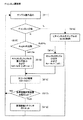
続いて、主サンプル列、副サンプル列の各サンプルの値を、予測誤差変換手段40が予測誤差値に変換する。あるサンプルにおける予測誤差値の算出は、時間的に過去に位置する直前の1つもしくは複数のサンプルの値を利用して行われる。本実施形態では、利用する直前のサンプル数を動的に変化させる手法を用いている。以下に、このような適応型線形予測符号化について説明する。予測誤差変換手段40により行われる適応型線形予測符号化の処理概要を図3のフローチャートに示す。まず、あらかじめ準備された複数の予測計算式を用いて、各予測計算式に対応した線形予測誤差を算出する(ステップS1)。具体的には、サンプル番号tの予測誤差を算出する予測計算式として、以下の〔数式1〕〜〔数式6〕を用意している。
【0016】
〔数式1〕
e0(t)=x(t)−e0(t−1)/2
【0017】
〔数式2〕
e1(t)=x(t)−a11・x(t−1)−e1(t−1)/2
【0018】
〔数式3〕
e2(t)=x(t)−a21・x(t−1)−a22・x(t−2)−e2(t−1)/2
【0019】
〔数式4〕
e3(t)=x(t)−a31・x(t−1)−a32・x(t−2)−a33・x(t−3)−e3(t−1)/2
【0020】
〔数式5〕
e4(t)=x(t)−a41・x(t−1)−a42・x(t−2)−a43・x(t−3)−a44・x(t−4)−e4(t−1)/2
【0021】
〔数式6〕
e5(t)=x(t)−a51・x(t−1)−a52・x(t−2)−a53・x(t−3)−a54・x(t−4)−a55・x(t−5)−e5(t−1)/2
【0022】
上記〔数式1〕〜〔数式6〕において、e0(t)〜e5(t)は各予測計算式による時刻tのサンプルにおける予測誤差であり、x(t)〜x(t−5)は時刻t〜t−5におけるサンプル値である。
【0023】
上記〔数式3〕における「a21・x(t−1)+a22・x(t−2)」、上記〔数式4〕における「a31・x(t−1)+a32・x(t−2)+a33・x(t−3)」、上記〔数式5〕における「a41・x(t−1)+a42・x(t−2)+a43・x(t−3)+a44・x(t−4)」、上記〔数式6〕における「a51・x(t−1)+a52・x(t−2)+a53・x(t−3)+a54・x(t−4)+a55・x(t−5)」は過去の2〜5個のサンプルに基づく線形予測成分である。この線形予測成分、および、直前のサンプルにおいて算出された予測誤差「e1(t−1)/2」〜「e5(t−1)/2」(誤差フィードバック成分)を用いて時刻tにおける予測誤差e0(t)〜e5(t)を算出する。
【0024】
上記の係数a11〜a55には初期値として、a11=1、a21=2、a22=−1、a31=3、a32=−3、a33=1、a41=4、a42=−6、a43=4、a44=−1、a51=5、a52=−10、a53=10、a54=−5、a55=1なる値が各々設定されているが、本実施形態では、これらの係数を動的に変化させる。具体的には、Levinson−Durvinのアルゴリズムを利用した以下の〔数式7〕を用いて係数a11〜a55を決定する。
【0025】
〔数式7〕
φ(k)=1/(N−K)・Σj=1,N−Kx(j)・x(j+k)
ki=−{φ(i)+Σj=1,i−1aj(i−1)・φ(i−j)}/E(i−1)
ai(i)=ki
aj(i)=aj(i−1)+ki・ai−j(i−1) ただし、1≦j≦i−1
E(i)=(1−ki 2)E(i−1)
【0026】
上記〔数式7〕において、φ(k)は、N個のサンプルx(j)(j=1,…,N)において、最大値K(上記例では5)の範囲でkサンプルシフトさせたサンプル列との自己相関値である。なお、NはKに対して十分大きな数値をとっている(例えばK=5の場合、N=32768)。〔数式7〕は、i=1からi=Kまで再帰的に繰り返し、最終的に得られたaj(K)が過去K個のサンプルに対応する係数になるとともに、各フェーズにおいて得られた中間結果であるaj(i)が係数aijとなる。ステップS1においては、上記〔数式7〕により決定した係数を用いて、〔数式1〕〜〔数式6〕の各計算式で計算を行うことになる。〔数式7〕による計算は、実際には後述するステップS7において行われるものである。また、係数を決定するには、過去の数サンプル分の値を必要とするので、初めのN−1サンプルについては、前述した初期係数で〔数式1〕〜〔数式6〕の計算を行うことになる。
【0027】
続いて、上記各予測計算式別の予測誤差値の絶対値の累積である累積誤差が最小となる線形予測誤差をそのサンプルの予測誤差として選出する(ステップS2)。ここでは、累積誤差という考え方を用いている。具体的には、各予測計算式〔数式1〕〜〔数式6〕により算出された予測誤差の過去のサンプルについての累積値をA0〜A5として設定する。そして、この累積誤差A0〜A5のうち、最小となるものに対応する予測誤差を選出する。例えば、A0〜A5のうち、A2が最小であったとする。この場合、〔数式3〕で算出された予測誤差e2(t)を符号化対象とする予測誤差e(t)として選出することになる。選出された予測誤差e(t)はサンプルの元の値x(t)と置き換えられて以降処理が行われることになる。
【0028】
続いて、累積誤差A0〜A5に各予測誤差e0(t)〜e5(t)の絶対値を加算する(ステップS3)。具体的には、以下の〔数式8〕に示すように、累積誤差値となる変数A0〜A5を更新していく。同時に、各サンプルの処理を行う度に、カウンタC1、C2を1つづつ加算していく処理を行う。
【0029】
〔数式8〕
A0←A0+|e0(t)|
A1←A1+|e1(t)|
A2←A2+|e2(t)|
A3←A3+|e3(t)|
A4←A4+|e4(t)|
A5←A5+|e5(t)|
【0030】
続いて、カウンタC1が所定回数を超えたかどうかの判定を行う(ステップS4)。本実施形態では、この所定回数を100回として設定している。すなわち、カウンタC1が100を超えたかどうかの判定を行う。
【0031】
この結果、カウンタが100を超えていたら、累積誤差を半分にする(ステップS5)。具体的には、以下の〔数式9〕に示すように、累積誤差となる変数A0〜A5を2で除算する。同時に、カウンタC1を0にリセットする。すなわち、ここでのA0〜A5は純粋な意味での累積誤差ではなく、累積誤差の移動平均となっている。本実施形態では、直前の最大100サンプルまでは累積されるが、それ以前のものは半分になるように処理する。これにより、時間的に離れたサンプルの影響が小さくなるようにしている。
【0032】
〔数式9〕
A0←(A0)/2
A1←(A1)/2
A2←(A2)/2
A3←(A3)/2
A4←(A4)/2
A5←(A5)/2
【0033】
続いて、カウンタC2が所定回数を超えたかどうかの判定を行う(ステップS6)。本実施形態では、この所定回数を32768回として設定している。すなわち、カウンタC2が32768を超えたかどうかの判定を行う。
【0034】
この結果、カウンタC2が32768を超えていたら、係数a11〜a55の再計算を行う(ステップS7)。具体的には、上記〔数式7〕を用いて、係数a11〜a55を計算し直すことになる。同時に、カウンタC2を0にリセットする。
【0035】
上記ステップS1〜ステップS7の処理を主サンプル列および副サンプル列のサンプルに渡って実行することにより、全サンプルの値が元の振幅値x(t)から対象誤差e(t)に置き換えられることになる。本実施形態では、特に、複数の予測式の係数を動的に変化させることにより、より精度の高い予測誤差を算出することが可能になる。
【0036】
次に、チャンネル間演算手段50が、予測誤差値が記録された各チャンネルの主サンプル、副サンプルに対して、チャンネル間の差分演算を行う。このチャンネル間差分演算の処理概要を図4のフローチャートに示す。まず、主サンプルを読み込む(ステップS11)。読み込んだ主サンプルがLチャンネルのものであれば、主サンプルの値をメモリに格納すると共に、次の極性処理手段60に出力する(ステップS12)。一方、読み込んだ主サンプルがRチャンネルのものであれば、ステップS13以降の処理を行う。なお、主サンプルは、各チャンネルのものが交互に読み込まれるので、判断を行う必要はない。例えば、サンプル番号t=1のLチャンネルのサンプルを読み込んだら、次はサンプル番号t=1のRチャンネルのサンプル、その次は、サンプル番号t=2のLチャンネルのサンプルというように順番が決まっているので、交互にステップS12の処理とステップS13以降の処理とを切替えるようにすれば良い。
【0037】
Rチャンネルのサンプルの場合は、変数AoとAdの比較を行う(ステップS13)。ここで、AoはRチャンネルのサンプル値の絶対値の累積であり、AdはRチャンネルとLチャンネルのサンプル値の差分の絶対値の累積である。変数Ao、Ad共に初期値は0である。ステップS13において、Ad≧Aoであれば、Rチャンネルのサンプルをそのままの値で、次の極性処理手段60に出力する(ステップS14)。さらに、累積値Aoを以下の〔数式10〕の第1式に示すように更新する。具体的には、Rチャンネルのサンプル値eRの絶対値を累積値Aoに加えることになる。
【0038】
ステップS13において、Ad<Aoであれば、上記ステップS12においてメモリに格納したLチャンネルのサンプルとの差分を算出し、差分値を次の極性処理手段60に出力する(ステップS15)。さらに、累積値Adを以下の〔数式10〕の第2式に示すように更新する。具体的には、RチャンネルとLチャンネルのサンプルの差分値eR−eLの絶対値を累積値Adに加えることになる。
【0039】
〔数式10〕
Ao←Ao+|eR|
Ad←Ad+|eR−eL|
【0040】
続いて、L、Rの1対のサンプルを処理したことを示すカウンタC3を1つ加算する(ステップS16)。
【0041】
続いて、カウンタが所定回数を超えたかどうかの判定を行う(ステップS17)。本実施形態では、この所定回数を100回として設定している。すなわち、カウンタC3が100を超えたかどうかの判定を行う。
【0042】
この結果、カウンタC3が100を超えていたら、累積値Ao、Adを半分にする(ステップS18)。具体的には、以下の〔数式11〕に示すように、累積値となる変数Ao、Adを2で除算する。同時に、カウンタCも半分にリセットする。すなわち、ここでの変数Ao、Adも上記〔数式8〕におけるA0〜A5と同様、純粋な意味での累積値ではなく、累積値の移動平均となっている。本実施形態では、直前の最大100サンプルまでは累積されるが、それ以前のものは半分になるように処理する。これにより、時間的に離れたサンプルの影響が小さくなるようにしている。
【0043】
〔数式11〕
Ao←Ao/2
Ad←Ad/2
C3←C3/2
【0044】
上記ステップS11〜ステップS18の処理を主サンプル列中の全主サンプルに渡って実行することにより、Rチャンネルの全サンプルの値が、Lチャンネルとの差分値に置き換えられることになる。ただし、上述の処理から明らかなように、累積値Ao、Adの大小関係によっては、Rチャンネルのサンプル値がそのまま記録されるサンプルも存在する。なお、チャンネル間演算手段50では、Lチャンネルのサンプルは、全てそのままの値で出力されることになる。主サンプル列中の各サンプルに対して処理を終えたら、副サンプルに対しても同様に処理を行う。なお、チャンネルが1つだけのモノラルの音響信号に対しては、チャンネル間演算手段50による処理は省略される。
【0045】
続いて、極性処理手段60が、各サンプルの正負極性処理を行う。上記予測誤差変換手段40およびチャンネル間演算手段50の処理により各サンプルの値は、振幅値から予測誤差に置き換えられると共に、Rチャンネルの値は、Lチャンネルとの差分に置き換えられたが、各サンプルのビット形式は、当初のままである。通常、コンピュータ等の計算機で演算される場合は、各データは32ビット単位で処理され、2の補数表現を用いて表現されている。これを、正負の符号付き絶対値表現に変換し、なおかつ、その絶対値部分を上位に1ビット移動させ、正負の符号ビットをLSB(最下位ビット)に移動させる。極性処理手段60によるビット構成の変換の様子を模式的に示すと図5のようになる。図5(a)は処理前のビット構成であり、図5(b)は処理後のビット構成である。このように正負の符号ビットをLSBに移動させるのは、後の可変長符号化手段70の処理で、各サンプルのビット長を検出し易くするためである。
【0046】
次に、可変長符号化手段70が、各サンプルを可変長に変換する処理を行っていく。本実施形態における可変長符号化は、一般にゴロム符号化と呼ばれる方式を採用している。具体的には、1サンプルを構成するビット成分を上位ビット成分と下位ビット成分に分け、下位ビット成分は変更を加えずそのままとし、上位ビット成分は、上位ビットだけを十進数変換した数値分のビット「0」を並べ、最後にセパレータビット「1」を加えた配列とする。例えば、8ビットのビット成分「00101000」を考えてみる。このとき、下位ビット成分を4ビットとすると、下位ビット成分は「1000」となる。上位ビットは「0010」であるため、これを十進数変換した「2」個分の「0」を配列して最後に「1」を加えた「001」に変換される。この結果、8ビットのビット列「00101000」は、7ビットのビット列「0011000」に変換されることになる。本実施形態では、変換の前後でビット成分を不変とする下位ビット成分のビット長を各サンプルで可変とするようにしている。
【0047】
以下、可変長符号化手段70が行う処理を具体的に説明していく。図6は可変長符号化の概要を示すフローチャートである。まず、過去のサンプルのビット長の移動平均である平均ビット長Bfを算出する(ステップS21)。平均ビット長Bfは、過去のビット長の累積値である累積ビット長RBを、過去のサンプル数を基にしたカウンタC4で除算することにより求められる。すなわち、Bf=RB/C4で算出される。累積ビット長RBは、初期状態では0であるので、t=1のサンプルを処理する場合には、t=1のサンプルのビット長Bd(t)を初期値として設定しておく。また、初期のカウンタC4=1と設定する。
【0048】
続いて、時刻tにおけるサンプルのビット長Bd(t)を算出する(ステップS22)。t=2以降のサンプルについては、平均ビット長Bfの算出後、サンプルのビット長Bd(t)を算出する。このビット長Bd(t)は、上記極性処理手段60によりビット構成の変換を行ったことにより算出し易くなっている。図5(b)に示したようなビット構成に変換したことにより、各サンプルのビット構成において先頭にビット「1」が出現したところからがビット長となる。次に、変更部のビット長Bvを算出する(ステップS23)。これは、上記サンプルのビット長Bd(t)から平均ビット長Bfを減じることにより算出される。続いて、データの符号出力を行う(ステップS24)。具体的には、上位Bvビットを十進数変換した数値分だけ「0」を出力した後、セパレータビット「1」を出力し、下位Bfビットを不変部として出力する。符号出力は、ハードディスク、CD−R等の外部記憶装置への記録として行われることになる。次に、累積ビット長RBにビット長Bd(t)を加算する(ステップS25)。同時に、各サンプルの処理を行う度に、カウンタC4を1つずつ加算していく処理を行う。続いて、カウンタC4が所定の数を超えたかどうかを判定する(ステップS26)。所定の数としては、ここでも100程度を設定している。そのため、カウンタ4が100を超えたかどうかを判断することになる。この結果、カウンタが100を超えていたら、累積ビット長RBを半分にする(ステップS27)。具体的には、累積ビット長となる変数RBを2で除算する。同時に、カウンタC4を1/2にする。
【0049】
上記のようにして、各サンプルについて可変ビット長での符号化が行われて行く。符号化により得られた可変長サンプルは、符号データとして出力される。なお、可変長符号化手段70には、上記のような処理を行うに先立ち量子化雑音成分を分離する機能を持たせておいても良い。具体的には、極性処理手段60による処理後の各サンプルの下位の所定数のビットを量子化雑音成分とみなして分離する。例えば各サンプルが16ビットで表現されている場合、本実施形態では、上位ビット12ビットと、下位ビット4ビットに分離する。この分離は、基本的に、A/D変換機等、音響信号をデジタル化する際に用いる回路の熱雑音を分離するために行う。そのため、熱雑音であると考えられる下位ビットを分離するのである。下位ビットとして、どの程度分離するかは、音源や利用した回路の特性によっても変化するが、通常量子化ビット数の1/4程度とすることが望ましい。したがって、ここでは、16ビットの1/4にあたる4ビットを下位ビットとして分離しているのである。
【0050】
ここで、上位ビットと下位ビットのデータ分離の様子を図7に模式的に示す。図7において、Hは上位ビットもしくは上位サンプルデータを示し、Lは下位ビットもしくは下位サンプルデータを示す。図7(a)は分離前のサンプルデータである。可変長符号化手段70により、サンプルデータは、図7(b)に示す上位サンプルデータと図7(c)に示す下位サンプルデータに分離された後処理されることになる。なお、上位ビットに含まれる符号ビットは、そのまま上位サンプルデータに含まれて分離される。このように、量子化雑音成分の分離を行った場合には、残りの上位ビットに対して、上記図6に示したフローチャートに従った可変長符号化が行われ、下位ビットについては、そのまま固定長で符号化が行われる。
【0051】
以上のようにして得られた符号データは、コンピュータに接続されたハードディスク等の記憶装置等に随時記憶され、その後、必要な記憶媒体に対応するフォーマットで記憶される。
【0052】
(第2の実施形態)
続いて、本発明第2の実施形態に係る符号化装置について説明する。図8は、本発明第2の実施形態に係る符号化装置の機能ブロック図である。図8において、図1に示した構成と同様の機能を有するものについては、同一符号を付して説明を省略する。第1の実施形態と異なる点は、信号平坦部処理手段80と相関フレーム検出手段90が加わったことである。図2において、信号平坦部処理手段80は、各チャンネルごとのサンプル列に対して、信号の値が一定である平坦部を検出し、効率的に符号化する機能を有する。相関フレーム検出手段90は、各サンプル列に対して、所定の区間をフレームとして設定した後、フレーム間で対応する全てのサンプル値が同一になっている相関フレームを検出し、時間的に後方(未来)に位置する相関フレームを削除する機能を有する。図8に示した装置は、実際には、コンピュータおよびコンピュータにインストールされた専用のソフトウェアプログラムにより実現される。
【0053】
続いて、図8に示した符号化装置の処理動作について説明する。まず、時系列信号入力手段10より上記のようなミックスされた音響信号を入力する。すると、チャンネル間演算手段50が上記図に示した手順に従って、チャンネル間の差分演算処理を行う。続いて、サンプル列再配置手段20が、上記図2に示したような処理で主サンプル列と副サンプル列に再配置する。その後、下位固定ビット削除手段30が各サンプルの下位ビットを削除する。
【0054】
次に、信号平坦部処理手段80が、信号平坦部の処理を行う。信号平坦部とは、同一の信号レベルが連続する部分のことをいう。特に信号レベルが「0」の無音部、および信号レベルの絶対値が最大の飽和部に現れることが多い。無音部は実際に無音であるか、音が非常に小さく記録されなかった場合に生じるが、飽和部は、信号の録音およびA/D変換の過程において生じる。無音部、飽和部またはそれ以外の同一信号レベルが連続する場合のいずれであっても、信号平坦部は、同一の信号レベルが所定の時間(所定のサンプル数)連続して記録される。このため、この部分は圧縮し易いデータになっている。具体的には、信号平坦部の先頭時刻位置と、同一信号レベルが続くサンプルの個数と、信号レベル(サンプル値)の3つの値を信号平坦部データとして各チャンネルのサンプル列と分離して記録する。各チャンネルのサンプル列からは、信号平坦部が削除される。これを模式的に示すと図9(a)(b)に示すようになる。図9(a)は、信号平坦部処理前のサンプル列である。図9(a)において、網掛けで示した部分は信号平坦部を示す。信号平坦部処理手段80の処理により、信号平坦部は元のサンプル列からは削除され、図9(b)に示すようになる。ただし、復号時に元通りに復元するために、分離された信号平坦部は、信号平坦部データとして図9(c)に示すような形式で記録しておく。
【0055】
信号平坦部データは、上述のように、信号平坦部ごとに、その先頭時刻(サンプル番号)、サンプル数、サンプル値の3属性で記録する。ここで、先頭時刻とは、信号の開始位置からの時刻であり、図9(c)の例では、先頭からのサンプル番号で記録している。このサンプル番号をサンプリング周波数で除算すれば、時刻に変換されることになる。サンプル数は、そのサンプル値がどの程度連続して続くかを示す情報である。なお、サンプル数の代わりに信号平坦部の終了時刻を記録するようにしても良い。サンプル値は、デジタル化された信号レベルを示している。符号付き16ビットで表現した場合は、最大値は「32767」、最小値は「−32768」となる。すなわち、「0」は無音部、「32767」および「−32768」は飽和部を示している。ただし、信号平坦部処理手段80は、信号平坦部を無条件には処理しない。本発明は、データの圧縮を目的としているため、サンプル列の削減分よりも信号平坦部データが大きくなると意味がないからである。したがって、信号平坦部となるサンプルが所定数以上連続する場合に限り信号平坦部データを作成して各チャンネルのサンプル列から分離するのである。
【0056】
続いて、各チャンネルのサンプル列に対して、相関フレーム検出手段90が、所定の区間長をもつフレームを設定して、設定されたフレーム間の比較を行う。本実施形態では、フレーム長をサンプル列の開始時刻から終了時刻までの全区間に渡って固定長としている。具体的には、1フレームを512サンプルとしている。相関フレーム検出手段90は、各チャンネルのサンプル列の先頭から512サンプルずつを1フレームとして設定し、フレーム間で全サンプルが一致する相関フレームを求めていくことになる。具体的な手順を図10のフローチャートに従って説明する。
【0057】
まず、相関フレーム検出手段90は、所定のサンプル数単位でフレーム化を行う(ステップS31)。本実施形態では、上述のようにフレーム長をサンプル列の開始時刻から終了時刻までの全区間に渡って固定長512サンプルとしている。相関フレーム検出手段90は、図11(a)に示すように、サンプル列の先頭から512サンプルずつを1フレームとして設定していくことになる。
【0058】
次に、各フレームに対して構成するサンプル値が全て一致するフレームを探索する。具体的には、図11(b)に示すように、まず、設定されたフレームのうち、時間的に最後尾のフレームを、相関フレームを探すための対象フレームとする。次に、所定の探索範囲内において、対象フレームの先頭サンプルの値と同一の値をもつサンプルを、時間的に遡りながら探索していく(ステップS32)。例えば、図12(a)に示すように、対象フレームがmT〜mT+511の512個のサンプルで構成されているとする。この場合、まず、対象フレームの先頭サンプルmTのサンプル値e(mT)と同一となるサンプルを探索していく。サンプルmT−1、サンプルmT−2と順に探索していく。なお、図12において、mは先頭からm番目のフレームであることを示し、Tはフレーム長(本実施形態では512サンプル)を示している。
【0059】
一致するサンプルtが見つかったら(ステップS33)、次に、そのサンプルtの次のサンプルt+1と対象フレームの2番目のサンプルmT+1が一致するかどうかを比較する。このようにしてサンプルの値が一致する限り後続するサンプル同士の比較を行っていく(ステップS34)。ステップS34においては、e(t+p)とe(mT+p)の値が一致する限り、処理を繰り返していく。例えば、図12(b)に示す例では、e(t)〜e(t+8)がe(mT)〜e(mT+8)と一致しているので、さらにp=9として、ステップS34の処理が続けられることになる。p=0〜p=511までの全てのe(t+p)とe(mT+p)が一致した場合(ステップS35)、そのサンプル列を対象フレームに対する相関フレームとし、相関フレームの先頭のサンプル番号と対象フレームの先頭のサンプル番号とを対応付けてフレーム相関データとして記録し、対象フレームを元のサンプル列から削除する(ステップS36)。対象フレームの全サンプルと一致しなければ、さらに対象フレームの先頭サンプルと値が一致するサンプルが存在するかどうかを時間的に遡りながら探索していく。所定のサンプル数分遡っても一致する相関フレームが存在しない場合は、その対象フレームに関する相関フレームの探索を中止し、対象フレームの直前のフレームを新たな対象フレームとして相関フレームの探索を行う。1つの対象フレームに対しての処理が終わったら、ステップS32に戻って、1つ直前のフレームを新たな対象フレームとして処理を続けていく(ステップS37)。このようにして、時系列信号の先頭時刻近辺に位置するフレームを除く全フレームを対象フレームとして相関フレームの検出処理を行う。
【0060】
サンプル列全体でみると、図11(c)に示すように対象フレームに対応する相関フレームが検出されたとすると、図11(d)に示すように対象フレームが削除されることになる。このとき、復号時に完全に復元できるように図11(e)に示すようなフレーム相関データが記録される。図11(e)に示すように、フレーム相関データには対象フレームの先頭のサンプル番号と相関フレームの先頭のサンプル番号が対応づけて記録される。
【0061】
以上、本発明の好適な実施形態について説明したが、本発明は上記実施形態に限定されず、種々の変形が可能である。例えば、上記実施形態では、主サンプルと副サンプルの出現比率が1対1のものについて説明したが、これ以外の比率のものでも良い。上記実施形態では、最初に48kHzでサンプリングしたものを96kHzに補間して作成した音響信号を扱ったので、主サンプルと副サンプルの出現比率が1対1となったが、例えば、最初に24kHzでサンプリングしたものを96kHzに補間すると、主サンプルと副サンプルの出現比率は1対3となる。このような音響信号を扱う場合には、サンプル列再配置手段20が、各サンプルを順番に1つの主サンプル列と3つの副サンプル列に順に振り分けるようにすれば良い。
【0062】
【発明の効果】
以上、説明したように本発明によれば、時系列信号を構成するサンプル列に対して、録音により作成された主サンプル列と、主サンプル列を補間処理することにより得られた副サンプル列を分離すると共に、前記副サンプル列中の各副サンプルの値を、近傍の主サンプルの平均値と当該副サンプルの値との差分値に変換するサンプル再配置を行い、主サンプル列、変換された副サンプル列それぞれに対して、線形予測誤差を算出し、主サンプル列および副サンプル列の値をそれぞれ予測誤差値に変換し、予測誤差値に変換された主サンプル列、副サンプル列を可変長で符号化するようにしたので、デジタル編集された高精細オーディオのワークデータを効率的に可逆圧縮することが可能となるという効果を奏する。
【図面の簡単な説明】
【図1】本発明第1の実施形態に係る時系列信号の符号化装置を示す機能ブロック図である。
【図2】サンプル列再配置手段20によるサンプルの再配置の様子を示す図である。
【図3】予測誤差変換手段40による処理を示すフローチャートである。
【図4】チャンネル間演算手段50による処理を示すフローチャートである。
【図5】極性処理手段60によるビット構成の変換の様子を示す図である。
【図6】可変長符号化手段70による処理を示すフローチャートである。
【図7】上位ビットと下位ビットのデータ分離の様子を示す図である。
【図8】本発明第2の実施形態に係る時系列信号の符号化装置を示す機能ブロック図である。
【図9】信号平坦部処理手段80による処理の様子を示す図である。
【図10】相関フレーム検出手段90による処理を示すフローチャートである。
【図11】相関フレーム検出手段90の処理による時系列信号全体の様子を示す図である。
【図12】相関フレーム検出手段90の処理により比較されるサンプルの様子を示す図である。
【符号の説明】
10・・・時系列信号入力手段
20・・・サンプル列再配置手段
30・・・下位固定ビット削除手段
40・・・予測誤差変換手段
50・・・チャンネル間演算手段
60・・・極性処理手段
70・・・可変長符号化手段
80・・・信号平坦部処理手段
90・・・相関フレーム検出手段[0001]
[Industrial applications]
INDUSTRIAL APPLICABILITY The present invention relates to music production fields such as music production, storage of acoustic data materials, relay of location materials, audio recording / reproduction using digital recording media such as CD / DVD, and analysis / diagnosis of biological signals in telemedicine. The present invention relates to a suitable data compression encoding technique.
[0002]
[Prior art]
Conventionally, various methods have been used for compressing an acoustic signal. MP3 (MPEG-1 / Layer3), AAC (MPEG-2 / Layer3) and the like have been put to practical use as a technique for compressing and encoding an audio signal. With such a compression encoding method, it is possible to treat an audio signal as small data, which contributes to the efficiency of data recording and transmission.
[0003]
Recently, not only lossy coding schemes such as MP3 and AAC as described above, but also lossless coding schemes that can be completely restored have been developed, and are used for sound material management (for example, Patent Document 1).
[0004]
[Patent Document 1]
JP 2000-821199 A
[0005]
[Problems to be solved by the invention]
When handling high-definition audio, sampling is performed with the sampling frequency or the number of quantization bits set higher than that of normal audio (music CD quality: sampling frequency 44.1 kHz,
[0006]
Therefore, in order to solve such a problem, the present invention provides an encoding device and a recording medium for a time-series signal capable of efficiently reversibly compressing high-definition audio work data in the course of digital editing. As an issue.
[0007]
[Means for Solving the Problems]
In order to solve the above-mentioned problem, in the present invention, for a time-series signal composed of a time-series sample sequence, an encoding device that compresses the amount of information so that all the sample sequences can be reproduced, In contrast, a main sample sequence created by recording and a sub-sample sequence obtained by interpolating the main sample sequence are separated, and the value of each sub-sample in the sub-sample sequence is replaced with a neighboring main sample sequence. A sample sequence rearrangement means for converting the average value of the sample and the value of the subsample into a difference value, calculating a linear prediction error for each of the main sample sequence and the converted subsample sequence, Prediction error conversion means for converting the values of the sample sequence and the sub-sample sequence into prediction error values, respectively, and encoding the main sample sequence and the sub-sample sequence converted into the prediction error value with a variable length. Characterized by being configured to have a variable length coding means.
[0008]
According to the present invention, the sample sequence constituting the time-series signal is rearranged into a main sample sequence obtained by recording and a sub-sample sequence obtained by interpolating the main sample sequence, and the main sample sequence and the sub-sample sequence are rearranged. Since each sample sequence is predictively coded and variable-length coded, work data of high-definition audio in the process of digital editing can be efficiently and reversibly compressed.
[0009]
BEST MODE FOR CARRYING OUT THE INVENTION
Hereinafter, embodiments of the present invention will be described in detail with reference to the drawings.
(1st Embodiment)
FIG. 1 is a configuration diagram showing a first embodiment of a time-series signal encoding apparatus according to the present invention. In FIG. 1,
[0010]
In FIG. 1, a time-series
[0011]
Next, the processing operation of the time-series signal encoding device shown in FIG. 1 will be described. In the present invention, a case will be described as an example in which work data in which a plurality of audio signals are mixed is handled as a time-series signal. As described above, such an audio signal includes both a normal audio signal having a sampling frequency of 48 kHz and a quantization bit number of 16 bits and a high-definition audio signal having a sampling frequency of 96 kHz and a quantization bit number of 24 bits. . A sound signal obtained by mixing sound signals having different sampling frequencies in this manner is handled by unifying the sampling frequency to a high-definition sound signal. In this case, a sound signal having a sampling frequency of 48 kHz is interpolated between the sound signals having a sampling frequency of 96 kHz with an average value of adjacent samples in order to match the number of samples.
[0012]
FIG. 2A schematically shows such an acoustic signal. In FIG. 2A, numbers in parentheses are sample numbers assigned in ascending order from 1, and x indicates a value of the sample. When such a time-series signal as a sample sequence is input from the time-series signal input means 10, the sample sequence rearrangement means 20 calculates the difference between the odd-numbered sample and the average value of the adjacent even-numbered samples. And the difference between the even-numbered sample and the average value of the adjacent odd-numbered sample is calculated. The sample rows at this time are schematically shown in FIGS. 2B and 2C, respectively. In the example of FIG. 2B, the even-numbered samples that are not subjected to the calculation are shown in the state of being moved temporally in the past, and in the example of FIG. .
[0013]
As a result of this difference operation, the one with the larger difference value is set as the sub-sample sequence, and the one with the smaller difference value is set as the main sample sequence. In the example of FIG. 2, each value of the latter half of the array of FIG.
The values in the second half of the array in FIG. 2C are compared. For example, when the odd-numbered sample is obtained by interpolation, the latter half value of the array shown in FIG. On the other hand, when the even-numbered samples are obtained by interpolation, the latter half value of the array shown in FIG. For example, when there are many values near 0 in the latter half of the array shown in FIG. 2B, the set of even-numbered samples is separated as the main sample sequence, and the set of odd-numbered samples is separated as the sub-sample sequence. In the processing of the sample sequence rearrangement means 20, the main sample is moved in the past in time and the sub-sample is moved in the future in time, as shown in FIGS. Alternatively, the main sample and the sub-sample may be handled separately. For example, if the odd number is a sub-sample, the main sample and the sub-sample are separated as shown in FIG. In the present invention, by performing linear prediction on a sample sequence including samples obtained by interpolating using original samples, the main sample Columns and subsample columns. Therefore, if linear prediction can be separately performed on the main sample sequence and the sub-sample sequence, even if only one sample sequence as shown in FIGS. May be two sample strings as shown in FIG.
[0014]
Next, the lower fixed
[0015]
Subsequently, the prediction error conversion means 40 converts the values of each sample of the main sample sequence and the sub-sample sequence into prediction error values. The calculation of the prediction error value for a certain sample is performed using the value of one or a plurality of samples located immediately before in the past in time. In the present embodiment, a method of dynamically changing the number of samples immediately before use is used. Hereinafter, such adaptive linear prediction encoding will be described. FIG. 3 is a flowchart showing an outline of processing of adaptive linear prediction encoding performed by the prediction error conversion means 40. First, using a plurality of prediction formulas prepared in advance, a linear prediction error corresponding to each prediction formula is calculated (step S1). Specifically, the following [Equation 1] to [Equation 6] are prepared as prediction calculation equations for calculating the prediction error of the sample number t.
[0016]
[Formula 1]
e0 (t) = x (t) -e0 (t-1) / 2
[0017]
[Formula 2]
e1 (t) = x (t) -a11X (t-1) -e1 (t-1) / 2
[0018]
[Equation 3]
e2 (t) = x (t) -a21X (t-1) -a22X (t-2) -e2 (t-1) / 2
[0019]
[Equation 4]
e3 (t) = x (t) -a31X (t-1) -a32X (t-2) -a33X (t-3) -e3 (t-1) / 2
[0020]
[Equation 5]
e4 (t) = x (t) -a41X (t-1) -a42X (t-2) -a43X (t-3) -a44X (t-4) -e4 (t-1) / 2
[0021]
[Equation 6]
e5 (t) = x (t) -a51X (t-1) -a52X (t-2) -a53X (t-3) -a54X (t-4) -a55X (t-5) -e5 (t-1) / 2
[0022]
In the above [Equation 1] to [Equation 6], e0 (t) to e5 (t) are prediction errors in the sample at time t by the respective prediction calculation formulas, and x (t) to x (t-5) are time Sample values at t to t-5.
[0023]
[A]21X (t-1) + a22X (t−2) ”and“ a ”in the above [
[0024]
The above coefficient a11~ A55Has an initial value of a11= 1, a21= 2, a22= -1, a31= 3, a32= -3, a33= 1, a41= 4, a42= -6, a43= 4, a44= -1, a51= 5, a52= -10, a53= 10, a54= -5, a55= 1 are set, but in the present embodiment, these coefficients are dynamically changed. Specifically, the coefficient a is calculated using the following [Equation 7] using the Levinson-Durvin algorithm.11~ A55To determine.
[0025]
[Equation 7]
φ (k) = 1 / (NK) −j = 1, NKx (j) · x (j + k)
ki= − {Φ (i) +}j = 1, i-1aj(I-1) · φ (ij)} / E (i-1)
ai(I) = ki
aj(I) = aj(I-1) + ki・ Aij(I-1) where 1≤j≤i-1
E (i) = (1-ki 2) E (i-1)
[0026]
In the above [Equation 7], φ (k) is a sample obtained by shifting k samples within a range of the maximum value K (5 in the above example) in N samples x (j) (j = 1,..., N). The autocorrelation value with the column. Note that N takes a sufficiently large value with respect to K (for example, when K = 5, N = 32768). [Equation 7] is recursively repeated from i = 1 to i = K, and finally obtained aj(K) becomes the coefficient corresponding to the past K samples, and a is an intermediate result obtained in each phase.j(I) is the coefficient aijBecomes In step S1, a calculation is performed using each of the formulas [1] to [6] using the coefficient determined by the above [7]. The calculation based on [Equation 7] is actually performed in step S7 described below. Further, since the values of several past samples are required to determine the coefficients, the calculation of [Equation 1] to [Equation 6] is performed for the first N-1 samples using the above initial coefficients. become.
[0027]
Next, a linear prediction error that minimizes the cumulative error, which is the accumulation of the absolute values of the prediction error values for each of the above-described prediction formulas, is selected as the prediction error of the sample (step S2). Here, the concept of accumulated error is used. Specifically, the accumulated values of the prediction errors calculated by the prediction calculation formulas [Formula 1] to [Formula 6] for the past samples are set as A0 to A5. Then, a prediction error corresponding to the smallest one of the accumulated errors A0 to A5 is selected. For example, it is assumed that A2 is the smallest among A0 to A5. In this case, the prediction error e2 (t) calculated by [Equation 3] is selected as the prediction error e (t) to be encoded. The selected prediction error e (t) is replaced with the original value x (t) of the sample, and the subsequent processing is performed.
[0028]
Subsequently, the absolute values of the prediction errors e0 (t) to e5 (t) are added to the accumulated errors A0 to A5 (step S3). Specifically, as shown in the following [Equation 8], variables A0 to A5 serving as accumulated error values are updated. At the same time, every time the processing of each sample is performed, the processing of adding the counters C1 and C2 one by one is performed.
[0029]
[Equation 8]
A0 ← A0 + | e0 (t) |
A1 ← A1 + | e1 (t) |
A2 ← A2 + | e2 (t) |
A3 ← A3 + | e3 (t) |
A4 ← A4 + | e4 (t) |
A5 ← A5 + | e5 (t) |
[0030]
Subsequently, it is determined whether or not the counter C1 has exceeded a predetermined number (step S4). In the present embodiment, the predetermined number is set to 100 times. That is, it is determined whether the counter C1 has exceeded 100.
[0031]
As a result, if the counter exceeds 100, the accumulated error is halved (step S5). Specifically, as shown in the following [Equation 9], variables A0 to A5 that are cumulative errors are divided by two. At the same time, the counter C1 is reset to 0. That is, A0 to A5 here are not accumulated errors in a pure sense, but are moving averages of the accumulated errors. In the present embodiment, up to the immediately preceding maximum of 100 samples are accumulated, but the previous samples are processed so as to be halved. Thereby, the influence of the samples separated in time is reduced.
[0032]
[Equation 9]
A0 ← (A0) / 2
A1 ← (A1) / 2
A2 ← (A2) / 2
A3 ← (A3) / 2
A4 ← (A4) / 2
A5 ← (A5) / 2
[0033]
Subsequently, it is determined whether or not the counter C2 has exceeded a predetermined number (step S6). In the present embodiment, the predetermined number is set to 32768 times. That is, it is determined whether the counter C2 has exceeded 32768.
[0034]
As a result, if the counter C2 exceeds 32768, the coefficient a11~ A55Is calculated again (step S7). Specifically, using the above [Equation 7], the coefficient a11~ A55Will be recalculated. At the same time, the counter C2 is reset to zero.
[0035]
By executing the processes of steps S1 to S7 over the samples of the main sample sequence and the sub-sample sequence, the values of all the samples are replaced from the original amplitude value x (t) by the target error e (t). become. In the present embodiment, in particular, it is possible to calculate a more accurate prediction error by dynamically changing coefficients of a plurality of prediction formulas.
[0036]
Next, the inter-channel calculation means 50 performs a difference calculation between the channels on the main sample and the sub-sample of each channel in which the prediction error value is recorded. FIG. 4 is a flowchart showing the outline of the process of calculating the difference between channels. First, a main sample is read (step S11). If the read main sample is for the L channel, the value of the main sample is stored in the memory and output to the next polarity processing means 60 (step S12). On the other hand, if the read main sample is for the R channel, the processing from step S13 is performed. Note that the main sample is read alternately for each channel, so there is no need to make a determination. For example, once the sample of the L channel with the sample number t = 1 is read, the order of the sample of the R channel with the sample number t = 1 is determined next, and then the sample of the L channel with the sample number t = 2. Therefore, the processing in step S12 and the processing after step S13 may be alternately switched.
[0037]
In the case of the R channel sample, the variables Ao and Ad are compared (step S13). Here, Ao is the accumulation of the absolute values of the sample values of the R channel, and Ad is the accumulation of the absolute values of the differences between the sample values of the R channel and the L channel. The initial values of both variables Ao and Ad are 0. If Ad ≧ Ao in step S13, the sample of the R channel is output as it is to the next polarity processing means 60 (step S14). Further, the accumulated value Ao is updated as shown in the following first equation of [Equation 10]. Specifically, the sample value e of the R channelRIs added to the accumulated value Ao.
[0038]
If Ad <Ao in step S13, the difference from the L channel sample stored in the memory in step S12 is calculated, and the difference value is output to the next polarity processing unit 60 (step S15). Further, the accumulated value Ad is updated as shown in the following Expression (10). Specifically, the difference value e between the samples of the R channel and the L channelR-ELIs added to the accumulated value Ad.
[0039]
[Equation 10]
Ao ← Ao + | eR|
Ad ← Ad + | eR-EL|
[0040]
Subsequently, the counter C3 that indicates that a pair of L and R samples has been processed is incremented by one (step S16).
[0041]
Subsequently, it is determined whether the counter has exceeded a predetermined number of times (step S17). In the present embodiment, the predetermined number is set to 100 times. That is, it is determined whether or not the counter C3 has exceeded 100.
[0042]
As a result, if the counter C3 exceeds 100, the cumulative values Ao and Ad are halved (step S18). Specifically, as shown in the following [Equation 11], variables Ao and Ad, which are cumulative values, are divided by two. At the same time, the counter C is also reset to half. That is, the variables Ao and Ad here are not cumulative values in a pure sense, but are moving averages of the cumulative values, similarly to A0 to A5 in [Equation 8]. In the present embodiment, up to the immediately preceding maximum of 100 samples are accumulated, but the previous samples are processed so as to be halved. Thereby, the influence of the samples separated in time is reduced.
[0043]
[Equation 11]
Ao ← Ao / 2
Ad ← Ad / 2
C3 ← C3 / 2
[0044]
By executing the processing of steps S11 to S18 over all the main samples in the main sample sequence, the values of all the samples of the R channel are replaced with the difference values from the L channel. However, as is apparent from the above-described processing, depending on the magnitude relationship between the accumulated values Ao and Ad, there is a sample in which the sample value of the R channel is recorded as it is. In the inter-channel calculation means 50, all the samples of the L channel are output as they are. When the processing is completed for each sample in the main sample sequence, the same processing is performed for the sub-samples. The processing by the inter-channel calculation means 50 is omitted for a monaural sound signal having only one channel.
[0045]
Subsequently, the polarity processing means 60 performs positive / negative processing on each sample. By the processing of the prediction error conversion means 40 and the inter-channel calculation means 50, the value of each sample was replaced from the amplitude value to the prediction error, and the value of the R channel was replaced by the difference from the L channel. Is unchanged from the original. Normally, when operated by a computer such as a computer, each data is processed in units of 32 bits and is expressed using a two's complement representation. This is converted into a positive / negative signed absolute value expression, and the absolute value portion is shifted one bit higher, and the positive / negative sign bit is shifted to the LSB (least significant bit). FIG. 5 schematically shows the conversion of the bit configuration by the polarity processing means 60. FIG. 5A shows a bit configuration before processing, and FIG. 5B shows a bit configuration after processing. The reason why the positive / negative sign bit is shifted to the LSB in this way is to make it easier to detect the bit length of each sample in the subsequent processing of the variable length coding means 70.
[0046]
Next, the variable length coding means 70 performs a process of converting each sample into a variable length. The variable length coding in the present embodiment employs a method generally called Golomb coding. More specifically, the bit components forming one sample are divided into upper bit components and lower bit components, the lower bit components are left unchanged, and the upper bit components are the numerical values obtained by converting only the upper bits into decimal numbers. Bits “0” are arranged, and a separator bit “1” is added at the end. For example, consider an 8-bit bit component "00101000". At this time, if the lower bit component is 4 bits, the lower bit component is “1000”. Since the upper bits are "0010", "2" pieces of "0" obtained by converting this number into decimal numbers are arranged, and are converted into "001" obtained by adding "1" at the end. As a result, the 8-bit bit string “00101000” is converted into a 7-bit bit string “00111000”. In the present embodiment, the bit length of the lower bit component that makes the bit component invariable before and after the conversion is made variable in each sample.
[0047]
Hereinafter, the processing performed by the variable
[0048]
Subsequently, the bit length Bd (t) of the sample at time t is calculated (step S22). For the samples after t = 2, after calculating the average bit length Bf, the bit length Bd (t) of the sample is calculated. The bit length Bd (t) can be easily calculated by converting the bit configuration by the polarity processing means 60. As a result of the conversion into the bit configuration as shown in FIG. 5B, the bit length starts from the bit “1” appearing at the head in the bit configuration of each sample. Next, the bit length Bv of the changing unit is calculated (Step S23). This is calculated by subtracting the average bit length Bf from the bit length Bd (t) of the sample. Subsequently, data sign output is performed (step S24). Specifically, after outputting “0” by the numerical value obtained by converting the upper Bv bits into a decimal number, a separator bit “1” is output, and the lower Bf bits are output as an invariable part. The code output is performed as recording on an external storage device such as a hard disk or a CD-R. Next, the bit length Bd (t) is added to the accumulated bit length RB (step S25). At the same time, every time the processing of each sample is performed, the processing of adding the counter C4 one by one is performed. Subsequently, it is determined whether the counter C4 has exceeded a predetermined number (step S26). As the predetermined number, about 100 is set here as well. Therefore, it is determined whether the
[0049]
As described above, encoding with a variable bit length is performed for each sample. The variable-length samples obtained by encoding are output as code data. Note that the variable length coding means 70 may have a function of separating the quantization noise component before performing the above processing. Specifically, a predetermined number of lower bits of each sample after the processing by the polarity processing means 60 are regarded as quantization noise components and separated. For example, when each sample is represented by 16 bits, in the present embodiment, the upper bits are separated into 12 bits and the lower bits are separated into 4 bits. This separation is basically performed to separate the thermal noise of a circuit used for digitizing an acoustic signal, such as an A / D converter. Therefore, lower bits considered to be thermal noise are separated. The degree to which the lower bits are separated depends on the characteristics of the sound source and the circuit used, but it is usually desirable to set the number of quantization bits to about 1/4. Therefore, in this case, 4 bits corresponding to 1/4 of 16 bits are separated as lower bits.
[0050]
Here, the state of data separation of upper bits and lower bits is schematically shown in FIG. In FIG. 7, H indicates upper bits or upper sample data, and L indicates lower bits or lower sample data. FIG. 7A shows sample data before separation. The variable length coding means 70 separates the sample data into upper sample data shown in FIG. 7B and lower sample data shown in FIG. Note that the sign bit included in the upper bits is directly included in the upper sample data and separated. As described above, when the quantization noise component is separated, the remaining upper bits are subjected to variable-length coding according to the flowchart shown in FIG. 6, and the lower bits are fixed as they are. Encoding is performed by length.
[0051]
The code data obtained as described above is stored as needed in a storage device such as a hard disk connected to a computer, and then stored in a format corresponding to a necessary storage medium.
[0052]
(Second embodiment)
Subsequently, an encoding device according to the second embodiment of the present invention will be described. FIG. 8 is a functional block diagram of an encoding device according to the second embodiment of the present invention. 8, components having the same functions as those in the configuration shown in FIG. 1 are denoted by the same reference numerals, and description thereof will be omitted. The difference from the first embodiment is that a signal flat part processing means 80 and a correlation frame detecting means 90 are added. In FIG. 2, the signal flat part processing means 80 has a function of detecting a flat part having a constant signal value for a sample sequence for each channel, and efficiently coding the same. After setting a predetermined section as a frame for each sample sequence, the correlation frame detection means 90 detects a correlation frame in which all the corresponding sample values are the same between frames, and detects the correlation frame backward (see FIG. It has a function of deleting the correlation frame located in the future. The apparatus shown in FIG. 8 is actually realized by a computer and a dedicated software program installed on the computer.
[0053]
Subsequently, the processing operation of the encoding device shown in FIG. 8 will be described. First, the mixed sound signal as described above is input from the time-series signal input means 10. Then, the inter-channel calculation means 50 performs a difference calculation process between the channels according to the procedure shown in the above figure. Subsequently, the sample sequence rearranging means 20 rearranges the sample sequence into the main sample sequence and the sub-sample sequence by the processing shown in FIG. After that, the lower fixed bit deleting means 30 deletes the lower bit of each sample.
[0054]
Next, the signal flat part processing means 80 performs processing of the signal flat part. The signal flat portion refers to a portion where the same signal level is continuous. In particular, it often appears in a silent part where the signal level is “0” and a saturated part where the absolute value of the signal level is the maximum. Silence occurs when the sound is actually silent or when the sound is not recorded very small, while saturation occurs during the signal recording and A / D conversion. Regardless of whether a silent portion, a saturated portion, or the other same signal level continues, the same signal level is continuously recorded for a predetermined time (a predetermined number of samples) in the signal flat portion. For this reason, this part is data that can be easily compressed. Specifically, the three values of the head time position of the signal flat portion, the number of samples following the same signal level, and the signal level (sample value) are recorded as signal flat portion data separately from the sample sequence of each channel. I do. The signal flat portion is deleted from the sample sequence of each channel. This is schematically shown in FIGS. 9A and 9B. FIG. 9A shows a sample sequence before the signal flat portion processing. In FIG. 9A, a shaded portion indicates a signal flat portion. By the processing of the signal flat part processing means 80, the signal flat part is deleted from the original sample sequence, as shown in FIG. 9B. However, in order to restore the original state at the time of decoding, the separated signal flat part is recorded as signal flat part data in a format as shown in FIG. 9C.
[0055]
As described above, the signal flat portion data is recorded for each signal flat portion with three attributes of the start time (sample number), the number of samples, and the sample value. Here, the head time is a time from the start position of the signal, and in the example of FIG. 9C, is recorded by the sample number from the head. If this sample number is divided by the sampling frequency, it will be converted to time. The sample number is information indicating how continuous the sample value continues. The end time of the signal flat portion may be recorded instead of the number of samples. The sample value indicates the digitized signal level. When represented by signed 16 bits, the maximum value is “32767” and the minimum value is “−32768”. That is, “0” indicates a silent part, and “32767” and “−32768” indicate a saturated part. However, the signal flat part processing means 80 does not unconditionally process the signal flat part. This is because the purpose of the present invention is to compress data, and it is meaningless if the signal flat portion data is larger than the reduction of the sample sequence. Therefore, only when the sample which becomes the signal flat portion continues for a predetermined number or more, the signal flat portion data is created and separated from the sample sequence of each channel.
[0056]
Subsequently, the correlation
[0057]
First, the correlation
[0058]
Next, a search is made for a frame in which all sample values constituting each frame match. Specifically, as shown in FIG. 11B, first, a temporally last frame among the set frames is set as a target frame for searching for a correlation frame. Next, within the predetermined search range, a sample having the same value as the value of the first sample of the target frame is searched while going back in time (step S32). For example, as shown in FIG. 12A, it is assumed that the target frame is composed of 512 samples of mT to mT + 511. In this case, first, a sample that is the same as the sample value e (mT) of the first sample mT of the target frame is searched for. The sample mT-1 and the sample mT-2 are sequentially searched. In FIG. 12, m indicates the m-th frame from the beginning, and T indicates the frame length (512 samples in this embodiment).
[0059]
When a matching sample t is found (step S33), it is next compared whether the next sample t + 1 of the sample t matches the second sample mT + 1 of the target frame. In this way, comparison between subsequent samples is performed as long as the values of the samples match (step S34). In step S34, the process is repeated as long as the values of e (t + p) and e (mT + p) match. For example, in the example shown in FIG. 12B, since e (t) to e (t + 8) match with e (mT) to e (mT + 8), the process of step S34 is continued with p = 9. Will be done. If all of e (t + p) and e (mT + p) from p = 0 to p = 511 match (step S35), the sample sequence is set as a correlation frame for the target frame, and the first sample number of the correlation frame and the target frame Is recorded as frame correlation data in association with the first sample number, and the target frame is deleted from the original sample sequence (step S36). If the sample does not match all the samples of the target frame, a search is further performed in time to determine whether there is a sample whose value matches the first sample of the target frame. If there is no matching correlation frame even after going back by the predetermined number of samples, the search for the correlation frame related to the target frame is stopped, and the search for the correlation frame is performed using the frame immediately before the target frame as a new target frame. When the processing for one target frame is completed, the process returns to step S32, and the processing is continued with the immediately preceding frame as a new target frame (step S37). In this way, the detection processing of the correlation frame is performed with all the frames except the frame located near the head time of the time series signal as the target frame.
[0060]
Looking at the entire sample sequence, assuming that a correlation frame corresponding to the target frame is detected as shown in FIG. 11C, the target frame is deleted as shown in FIG. 11D. At this time, frame correlation data as shown in FIG. 11 (e) is recorded so that it can be completely restored at the time of decoding. As shown in FIG. 11E, the head sample number of the target frame and the head sample number of the correlation frame are recorded in the frame correlation data in association with each other.
[0061]
The preferred embodiment of the present invention has been described above, but the present invention is not limited to the above embodiment, and various modifications are possible. For example, in the above-described embodiment, the case where the appearance ratio of the main sample and the sub-sample is 1 to 1 has been described, but another ratio may be used. In the above embodiment, the sound signal created by first interpolating the sampled signal at 48 kHz to 96 kHz was used, so that the appearance ratio of the main sample and the sub-sample was 1: 1. When the sampled sample is interpolated to 96 kHz, the appearance ratio of the main sample and the sub-sample becomes 1: 3. When dealing with such an acoustic signal, the sample sequence rearranging means 20 may divide each sample into one main sample sequence and three sub-sample sequences in order.
[0062]
【The invention's effect】
As described above, according to the present invention, for a sample sequence constituting a time-series signal, a main sample sequence created by recording and a sub-sample sequence obtained by interpolating the main sample sequence are described. Separating and performing a sample rearrangement to convert the value of each sub-sample in the sub-sample sequence into a difference between the average value of the nearby main sample and the value of the sub-sample, the main sample sequence is converted. A linear prediction error is calculated for each sub-sample sequence, the values of the main sample sequence and the sub-sample sequence are converted into prediction error values, and the main sample sequence and the sub-sample sequence converted into the prediction error values are variable-length. Since the encoding is performed by using, the digitally edited high-definition audio work data can be efficiently reversibly compressed.
[Brief description of the drawings]
FIG. 1 is a functional block diagram showing an apparatus for encoding a time-series signal according to a first embodiment of the present invention.
FIG. 2 is a diagram showing a state of sample rearrangement by a sample
FIG. 3 is a flowchart showing processing by a prediction
FIG. 4 is a flowchart showing processing by an inter-channel calculation means 50;
FIG. 5 is a diagram showing a state of conversion of a bit configuration by a
FIG. 6 is a flowchart showing a process performed by a variable-
FIG. 7 is a diagram showing a state of data separation of upper bits and lower bits.
FIG. 8 is a functional block diagram illustrating a time-series signal encoding device according to a second embodiment of the present invention.
FIG. 9 is a diagram showing a state of processing by a signal flat part processing means 80;
FIG. 10 is a flowchart illustrating a process performed by a correlation
FIG. 11 is a diagram showing a state of an entire time-series signal by processing of a correlation
FIG. 12 is a diagram showing a state of samples compared by the processing of the correlation frame detection means 90.
[Explanation of symbols]
10 time-series signal input means
20 ... sample row rearrangement means
30... Lower fixed bit deleting means
40 ... Prediction error conversion means
50: Channel calculation means
60 ... polarity processing means
70 ... variable length coding means
80 ... Signal flat part processing means
90 ... correlation frame detecting means
Claims (11)
前記サンプル列に対して、録音信号をサンプリングすることにより得られた主サンプル列と、主サンプル列を補間処理することにより得られた副サンプル列を分離すると共に、前記副サンプル列中の各副サンプルの値を、近傍の主サンプルの平均値と当該副サンプルの値との差分値に変換するサンプル列再配置手段と、
前記主サンプル列、前記変換された副サンプル列それぞれに対して、線形予測誤差を算出し、前記主サンプル列および前記副サンプル列の値をそれぞれ予測誤差値に変換する予測誤差変換手段と、
前記予測誤差値に変換された主サンプル列、副サンプル列を可変長で符号化する可変長符号化手段と、
を有することを特徴とする時系列信号の符号化装置。A coding apparatus that compresses the amount of information so that all the sample sequences can be reproduced with respect to a time-series signal including a time-series sample sequence,
For the sample sequence, a main sample sequence obtained by sampling a recording signal and a sub-sample sequence obtained by interpolating the main sample sequence are separated, and each sub-sample sequence in the sub-sample sequence is separated. Sample sequence rearrangement means for converting the value of the sample into a difference between the average value of the nearby main sample and the value of the subsample;
Prediction error conversion means for calculating a linear prediction error for each of the main sample sequence and the converted sub-sample sequence, and converting the values of the main sample sequence and the sub-sample sequence into prediction error values,
The main sample sequence converted to the prediction error value, a variable length encoding means for encoding the sub-sample sequence with a variable length,
An encoding device for a time-series signal, comprising:
前記サンプル列再配置手段は、前記サンプル列の偶数番目に位置するサンプルの値が前後の奇数番目に位置するサンプル列の平均値に近い場合に、奇数番目に位置するサンプルを主サンプル列、偶数番目に位置するサンプルを副サンプル列に分離するものであり、
前記サンプル列の奇数番目に位置するサンプルの値が前後の偶数番目に位置するサンプル列の平均値に近い場合に、偶数番目に位置するサンプルを主サンプル列、奇数番目に位置するサンプルを副サンプル列に分離するものであることを特徴とする時系列信号の符号化装置。In claim 1,
The sample sequence rearrangement means, when a value of an even-numbered sample sequence of the sample sequence is close to the average value of the preceding and following odd-numbered sample sequence, the odd-numbered sample is a main sample sequence, an even-numbered sample sequence. To separate the sample located at the
When the value of an odd-numbered sample in the sample sequence is close to the average value of the preceding and following even-numbered sample sequences, the even-numbered sample is a main sample sequence, and the odd-numbered sample is a sub-sample. An encoding device for a time-series signal, which is separated into columns.
前記主サンプル列および前記副サンプル列変換手段による処理後の副サンプル列に対して、下位の所定数のビット成分を削除する下位固定ビット削除手段を有し、当該下位固定ビット削除手段による処理後のサンプル列に対して前記予測誤差変換手段が処理を行うものであることを特徴とする時系列信号の符号化装置。In claim 1,
A low-order fixed bit deletion unit that deletes a predetermined number of lower-order bit components from the main sample sequence and the sub-sample sequence processed by the sub-sample sequence conversion unit; Wherein the prediction error conversion means performs processing on the sample sequence of (1).
前記サンプル列が同一時刻に複数の値をもつ複数のチャンネルで構成されている場合、チャンネル間の同一時刻におけるサンプル同士の差分を算出し、いずれかのチャンネルのサンプル列を前記算出された差分値で更新するようにしたチャンネル間演算手段をさらに有することを特徴とする時系列信号の符号化装置。In claim 1,
When the sample sequence is composed of a plurality of channels having a plurality of values at the same time, the difference between the samples at the same time between the channels is calculated, and the sample sequence of any channel is calculated as the calculated difference value. A time-series signal encoding apparatus, further comprising an inter-channel calculation means for updating the time-series signal.
前記サンプル列の中で、サンプルの値が連続して同一値になっているサンプルを抽出し、前記サンプル列から削除すると共に、削除したサンプルの先頭時間位置と、サンプル個数と、サンプル値の3つの値を符号化する信号平坦部処理手段を、前記予測誤差変換手段の前段に有することを特徴とする時系列信号の符号化装置。In claim 1,
In the sample sequence, a sample in which the value of the sample is continuously the same is extracted and deleted from the sample sequence, and the start time position of the deleted sample, the number of samples, and the sample value are calculated. An encoding apparatus for a time-series signal, comprising signal flat part processing means for encoding two values at a stage preceding the prediction error conversion means.
前記サンプル列の中から所定の個数のサンプル列で構成されるフレームと同一内容のフレームが時間的に過去に存在する場合に、未来に位置するフレームを削除し、両フレームの先頭時間位置と、フレームを構成するサンプル個数を符号化する相関フレーム検出手段を、前記予測誤差変換手段の前段に有することを特徴とする時系列信号の符号化装置。In claim 1,
If a frame having the same content as a frame composed of a predetermined number of sample sequences exists in the past in the sample sequence, the frame located in the future is deleted, and the start time position of both frames, An apparatus for encoding a time-series signal, comprising: a correlation frame detecting means for encoding the number of samples forming a frame, at a stage preceding the prediction error converting means.
前記予測誤差変換手段は、前記主サンプル列および副サンプル列に対して、時間的に過去のサンプル列から、複数の予測計算式に基づいて、複数の予測誤差値の候補を算出し、その中から符号化対象の予測誤差値を選別するものであることを特徴とする時系列信号の符号化装置。In claim 1,
The prediction error conversion means calculates a plurality of prediction error value candidates for the main sample sequence and the sub-sample sequence from a temporally past sample sequence based on a plurality of prediction calculation formulas. A time-series signal encoding apparatus for selecting a prediction error value to be encoded from the data.
前記複数の予測計算式の線形係数を、所定のサンプル数ごとに更新することを特徴とする時系列信号の符号化装置。In claim 7,
An apparatus for encoding a time-series signal, wherein the linear coefficients of the plurality of prediction formulas are updated every predetermined number of samples.
前記予測誤差に変換されたサンプル値の絶対値に対して、全体を1ビット上位にずらし、正負符号を最下位1ビットに挿入する極性処理手段を、前記可変長符号化手段の前段に有することを特徴とする時系列信号の符号化装置。In claim 1,
Polarity processing means for shifting the whole of the absolute value of the sample value converted to the prediction error by one bit higher and inserting a sign into the least significant one bit is provided before the variable length coding means. A time-series signal encoding apparatus characterized by the above-mentioned.
前記可変長符号化手段は、前記予測誤差値に変換された各サンプルのビット成分のうち、下位のビット成分をそのままのビット成分で符号化し、残りの上位ビット成分に対してビット成分を変更して符号化を行うものであることを特徴とする時系列信号の符号化装置。In claim 1,
The variable-length encoding means encodes lower-order bit components as they are among bit components of each sample converted to the prediction error value, and changes bit components for the remaining upper-order bit components. A time-series signal encoding apparatus for performing encoding by using a time-series signal.
Priority Applications (1)
| Application Number | Priority Date | Filing Date | Title |
|---|---|---|---|
| JP2003055114A JP4170795B2 (en) | 2003-03-03 | 2003-03-03 | Time-series signal encoding apparatus and recording medium |
Applications Claiming Priority (1)
| Application Number | Priority Date | Filing Date | Title |
|---|---|---|---|
| JP2003055114A JP4170795B2 (en) | 2003-03-03 | 2003-03-03 | Time-series signal encoding apparatus and recording medium |
Publications (2)
| Publication Number | Publication Date |
|---|---|
| JP2004266587A true JP2004266587A (en) | 2004-09-24 |
| JP4170795B2 JP4170795B2 (en) | 2008-10-22 |
Family
ID=33119210
Family Applications (1)
| Application Number | Title | Priority Date | Filing Date |
|---|---|---|---|
| JP2003055114A Expired - Fee Related JP4170795B2 (en) | 2003-03-03 | 2003-03-03 | Time-series signal encoding apparatus and recording medium |
Country Status (1)
| Country | Link |
|---|---|
| JP (1) | JP4170795B2 (en) |
Cited By (5)
| Publication number | Priority date | Publication date | Assignee | Title |
|---|---|---|---|---|
| JP2009031377A (en) * | 2007-07-25 | 2009-02-12 | Nec Electronics Corp | Audio data processor, bit width conversion method and bit width conversion device |
| JP2010506226A (en) * | 2006-10-13 | 2010-02-25 | ギャラクシー ステューディオス エヌヴェー | Method and encoder for combining digital data sets, decoding method and decoder for combined digital data sets, and recording medium for storing combined digital data sets |
| CN103294729A (en) * | 2012-03-05 | 2013-09-11 | 富士通株式会社 | Method and equipment for processing and predicting time sequence containing sample points |
| JP2018512613A (en) * | 2015-02-27 | 2018-05-17 | アウロ テクノロジーズ エンフェー. | Encoding and decoding digital data sets |
| CN110487268A (en) * | 2019-07-17 | 2019-11-22 | 哈尔滨工程大学 | A kind of three increment sculling Error Compensation Algorithm of interpolation inputted based on angular speed and specific force |
-
2003
- 2003-03-03 JP JP2003055114A patent/JP4170795B2/en not_active Expired - Fee Related
Cited By (6)
| Publication number | Priority date | Publication date | Assignee | Title |
|---|---|---|---|---|
| JP2010506226A (en) * | 2006-10-13 | 2010-02-25 | ギャラクシー ステューディオス エヌヴェー | Method and encoder for combining digital data sets, decoding method and decoder for combined digital data sets, and recording medium for storing combined digital data sets |
| JP2009031377A (en) * | 2007-07-25 | 2009-02-12 | Nec Electronics Corp | Audio data processor, bit width conversion method and bit width conversion device |
| CN103294729A (en) * | 2012-03-05 | 2013-09-11 | 富士通株式会社 | Method and equipment for processing and predicting time sequence containing sample points |
| JP2018512613A (en) * | 2015-02-27 | 2018-05-17 | アウロ テクノロジーズ エンフェー. | Encoding and decoding digital data sets |
| CN110487268A (en) * | 2019-07-17 | 2019-11-22 | 哈尔滨工程大学 | A kind of three increment sculling Error Compensation Algorithm of interpolation inputted based on angular speed and specific force |
| CN110487268B (en) * | 2019-07-17 | 2023-01-03 | 哈尔滨工程大学 | Interpolation three-subsample sculling effect error compensation method based on angular rate and specific force input |
Also Published As
| Publication number | Publication date |
|---|---|
| JP4170795B2 (en) | 2008-10-22 |
Similar Documents
| Publication | Publication Date | Title |
|---|---|---|
| JP4374448B2 (en) | Multi-channel signal encoding method, decoding method thereof, apparatus, program and recording medium thereof | |
| JP4049791B2 (en) | Floating-point format digital signal lossless encoding method, decoding method, each apparatus, and each program | |
| JPWO2006019117A1 (en) | Multi-channel signal encoding method, decoding method thereof, apparatus, program and recording medium thereof | |
| JP3960932B2 (en) | Digital signal encoding method, decoding method, encoding device, decoding device, digital signal encoding program, and decoding program | |
| JP4761251B2 (en) | Long-term prediction encoding method, long-term prediction decoding method, these devices, and program thereof | |
| JP4170795B2 (en) | Time-series signal encoding apparatus and recording medium | |
| JP4357852B2 (en) | Time series signal compression analyzer and converter | |
| JP4249540B2 (en) | Time-series signal encoding apparatus and recording medium | |
| JP4736331B2 (en) | Acoustic signal playback device | |
| JP4139704B2 (en) | Time series signal encoding apparatus and decoding apparatus | |
| JP4184817B2 (en) | Time series signal encoding method and apparatus | |
| JP2004198559A (en) | Encoding method and decoding method for time-series signal | |
| JP4109124B2 (en) | Time series signal encoding device | |
| JP4139697B2 (en) | Time series signal encoding method and apparatus | |
| JP2006211243A (en) | Device and method for digital signal encoding | |
| JP3889738B2 (en) | Inverse quantization apparatus, audio decoding apparatus, image decoding apparatus, inverse quantization method, and inverse quantization program | |
| JP4319895B2 (en) | Time series signal encoding device | |
| JP2005166216A (en) | Reproducing apparatus of sound signal | |
| JPH11109996A (en) | Voice coding device, voice coding method and optical recording medium recorded with voice coding information and voice decoding device | |
| JP3387092B2 (en) | Audio coding device | |
| JP2004070120A (en) | Encoding device, decoding device and recording medium for time-series signal | |
| JP2007214741A (en) | Image data compression apparatus, image display apparatus, image data compression method, image display method, image data compression program, image display program, and storage medium | |
| JP2005215162A (en) | Reproducing device of acoustic signal | |
| JP3387094B2 (en) | Audio coding method | |
| Skyttberg | Digital Representation of Audio |
Legal Events
| Date | Code | Title | Description |
|---|---|---|---|
| A621 | Written request for application examination |
Free format text: JAPANESE INTERMEDIATE CODE: A621 Effective date: 20060227 |
|
| A977 | Report on retrieval |
Free format text: JAPANESE INTERMEDIATE CODE: A971007 Effective date: 20080509 |
|
| A131 | Notification of reasons for refusal |
Free format text: JAPANESE INTERMEDIATE CODE: A131 Effective date: 20080529 |
|
| A521 | Request for written amendment filed |
Free format text: JAPANESE INTERMEDIATE CODE: A523 Effective date: 20080703 |
|
| TRDD | Decision of grant or rejection written | ||
| A01 | Written decision to grant a patent or to grant a registration (utility model) |
Free format text: JAPANESE INTERMEDIATE CODE: A01 Effective date: 20080723 |
|
| A01 | Written decision to grant a patent or to grant a registration (utility model) |
Free format text: JAPANESE INTERMEDIATE CODE: A01 |
|
| A61 | First payment of annual fees (during grant procedure) |
Free format text: JAPANESE INTERMEDIATE CODE: A61 Effective date: 20080807 |
|
| FPAY | Renewal fee payment (event date is renewal date of database) |
Free format text: PAYMENT UNTIL: 20110815 Year of fee payment: 3 |
|
| R150 | Certificate of patent or registration of utility model |
Ref document number: 4170795 Country of ref document: JP Free format text: JAPANESE INTERMEDIATE CODE: R150 Free format text: JAPANESE INTERMEDIATE CODE: R150 |
|
| FPAY | Renewal fee payment (event date is renewal date of database) |
Free format text: PAYMENT UNTIL: 20110815 Year of fee payment: 3 |
|
| FPAY | Renewal fee payment (event date is renewal date of database) |
Free format text: PAYMENT UNTIL: 20120815 Year of fee payment: 4 |
|
| FPAY | Renewal fee payment (event date is renewal date of database) |
Free format text: PAYMENT UNTIL: 20120815 Year of fee payment: 4 |
|
| FPAY | Renewal fee payment (event date is renewal date of database) |
Free format text: PAYMENT UNTIL: 20130815 Year of fee payment: 5 |
|
| LAPS | Cancellation because of no payment of annual fees |