EP4517604A1 - Programm zur partitionierung von mehrfach-qubit-observables, verfahren zur partitionierung von mehrfach-qubit-observables und informationsverarbeitungsvorrichtung - Google Patents
Programm zur partitionierung von mehrfach-qubit-observables, verfahren zur partitionierung von mehrfach-qubit-observables und informationsverarbeitungsvorrichtung Download PDFInfo
- Publication number
- EP4517604A1 EP4517604A1 EP22940108.8A EP22940108A EP4517604A1 EP 4517604 A1 EP4517604 A1 EP 4517604A1 EP 22940108 A EP22940108 A EP 22940108A EP 4517604 A1 EP4517604 A1 EP 4517604A1
- Authority
- EP
- European Patent Office
- Prior art keywords
- observables
- clique
- processing
- partitioning
- group
- Prior art date
- Legal status (The legal status is an assumption and is not a legal conclusion. Google has not performed a legal analysis and makes no representation as to the accuracy of the status listed.)
- Pending
Links
Images


Classifications
-
- G—PHYSICS
- G06—COMPUTING OR CALCULATING; COUNTING
- G06N—COMPUTING ARRANGEMENTS BASED ON SPECIFIC COMPUTATIONAL MODELS
- G06N5/00—Computing arrangements using knowledge-based models
- G06N5/01—Dynamic search techniques; Heuristics; Dynamic trees; Branch-and-bound
-
- G—PHYSICS
- G06—COMPUTING OR CALCULATING; COUNTING
- G06N—COMPUTING ARRANGEMENTS BASED ON SPECIFIC COMPUTATIONAL MODELS
- G06N10/00—Quantum computing, i.e. information processing based on quantum-mechanical phenomena
- G06N10/60—Quantum algorithms, e.g. based on quantum optimisation, quantum Fourier or Hadamard transforms
-
- G—PHYSICS
- G06—COMPUTING OR CALCULATING; COUNTING
- G06N—COMPUTING ARRANGEMENTS BASED ON SPECIFIC COMPUTATIONAL MODELS
- G06N10/00—Quantum computing, i.e. information processing based on quantum-mechanical phenomena
- G06N10/20—Models of quantum computing, e.g. quantum circuits or universal quantum computers
Definitions
- the present invention relates to a partitioning program for multi-qubit observables, a partitioning method for the multi-qubit observables, and an information processing device.
- a qubit electronic information referred to as a qubit is used.
- the qubit may take a superposition state of "0" and "1". Furthermore, it is also possible to create a quantum entanglement state with a plurality of qubits.
- the quantum computer may obtain a solution of a complex problem in a short time by calculating all possibilities simultaneously and in parallel using these superposition state and quantum entanglement state.
- an algorithm for solving a problem in the quantum computer is referred to as a quantum algorithm
- an algorithm for solving a problem in the classical computer is referred to as a classical algorithm.
- a quantum algorithm an algorithm for solving a problem in the classical computer
- a classical algorithm an algorithm for solving a problem in the classical computer
- steps (exponential time) of about M M times is needed to obtain a solution
- steps (polynomial time) of only about M 2 times is needed (M is a natural number indicating a magnitude of the problem).
- Examples of a problem that may be calculated in a short time by the quantum computer include a Deutsch-Jozsa algorithm, a Shor algorithm, and the like.
- the quantum state it is needed to read not only a value of a z axis of the Bloch sphere but also values of an x axis and a y axis.
- the value of the x axis or the y axis may be measured by performing an operation of converting the value into the value of the z axis before measurement, and reading the value after the conversion operation. Note that, when qubits are measured, a superposition state of the qubits is destroyed. Therefore, in order to completely know the quantum state, quantum calculation for measurement of each of the x axis, the y axis, and the z axis is repeatedly executed.
- a state of one or a plurality of qubits is represented by using a plurality of observables.
- n is a natural number
- the state of the qubit may be completely known.
- the expected value for each observable is obtained, basically, one quantum circuit is created for each observable.
- 10 4 to 10 5 times of measurement are performed per observable.
- an optimization device that suppresses an increase in a calculation amount when a combinatorial optimization problem is divided for calculation has been proposed.
- An optimization device capable of improving calculation efficiency when a combinatorial optimization problem is divided for calculation has also been proposed.
- VQE variational quantum eigensolver
- partitioning In simultaneous measurement of expected values of a plurality of observables, partitioning generates sets (cliques) of observables that may be simultaneously measured. Each observable is included in any one of the cliques.
- the simultaneous measurement of the expected values by the quantum computer is performed for each of the predetermined number of observables included in the same clique. In this case, the smaller the number of cliques, the more efficient the measurement of the state of the qubit. As the number of observables to be measured increases, a calculation amount for generating a clique including more observables becomes enormous. In that case, for example, by performing the partitioning using an Ising machine that calculates a ground state of an Ising model, it is possible to accelerate the partitioning.
- the Ising machine may not perform the partitioning for all the observables.
- the number of observables included in one clique is reduced and the number of cliques to be generated is increased.
- an object of the present case is to reduce the number of cliques generated in partitioning.
- a partitioning program for multi-qubit observables for causing a computer to execute the following processing.
- a computer causes an Ising machine to calculate a solution of a first combinatorial optimization problem that searches for a combination that includes more observables, which is a combination of observables in a first group that includes at least two observables of a plurality of observables to be measured, and which satisfies a condition that simultaneous measurement of expected values is possible for optional two observables included in the combination.
- the computer generates a first clique that indicates a combination of observables indicated in the solution of the first combinatorial optimization problem.
- the computer generates a second group that includes a predetermined number of observables not included in the first clique based on the number of observables in the first clique, for which simultaneous measurement of expected values is possible for each observable not included in the first clique.
- the computer causes the Ising machine to calculate a solution of a second combinatorial optimization problem that searches for a combination that includes more observables, which is a combination of observables in a union of the first clique and the second group, and which satisfies a condition that simultaneous measurement of the expected values is possible for optional two observables included in the combination.
- the computer generates a second clique that indicates a combination of observables indicated in the solution of the second combinatorial optimization problem.
- the computer repeats, until a predetermined end condition is satisfied, processing of updating the observables included in the first clique with the observables included in the second clique, the processing of generating the second group, the processing of causing the Ising machine to calculate the solution of the second combinatorial optimization problem, and the processing of generating the second clique.
- the number of cliques generated in partitioning may be reduced.
- the first embodiment is a partitioning method for multi-qubit observables that alleviates a limit on the number of observables in a case where a clique is generated using an Ising machine (including an annealing-type computer).
- FIG. 1 is a diagram illustrating an example of the partitioning method for the multi-qubit observables according to the first embodiment.
- FIG. 1 an example of a case where processing of the partitioning method for the multi-qubit observables is performed by an information processing device 10 is illustrated.
- the information processing device 10 may perform the partitioning method for the multi-qubit observables by, for example, executing a partitioning program for the multi-qubit observables.
- the information processing device 10 includes a storage unit 11 and a processing unit 12.
- the storage unit 11 is, for example, a memory or a storage device included in the information processing device 10.
- the processing unit 12 is, for example, a processor or an arithmetic circuit included in the information processing device 10.
- the information processing device 10 performs partitioning of a plurality of observables representing a states of a qubit.
- the information processing device 10 is coupled to an Ising machine 1, and determines observables to be included in a clique using the Ising machine 1 at the time of partitioning.
- the Ising machine 1 allocates calculation bits to each of observables to be subjected to the processing.
- a value of each bit represents whether or not to include a corresponding observable in a clique. Therefore, in order to perform the clique generation processing, the number of observables included in a set of the observables to be subjected to the processing is needed to be equal to or less than the number of bits used for calculation by the Ising machine 1.
- the storage unit 11 stores an observable group 2.
- the observable group 2 includes a plurality of observables to be measured among a plurality of observables representing states of a plurality of qubits.
- circles in the observable group 2 represent the observables to be measured.
- the observables to be measured are determined according to a problem to be solved using a quantum computer. For example, in a case where it is desired to completely know states of n qubits, 4 n -1 observables are included in the observable group 2.
- the processing unit 12 performs partitioning that divides the observable group 2 into a plurality of cliques.
- the processing unit 12 generates the cliques one by one.
- the processing unit 12 executes the clique generation processing of two or more stages in order to generate one clique.
- the processing unit 12 generates a first group 3 including at least two observables among the plurality of observables to be measured.
- the first group 3 includes, for example, observables optionally selected from the observable group 2.
- the processing unit 12 selects the same number of observables as the number of bits that may be used for calculation by the Ising machine 1 from the observable group 2, and includes the selected observables in the first group 3.
- the processing unit 12 causes the Ising machine 1 to calculate a solution of a first combinatorial optimization problem that searches for a combination of observables in the first group 3, which includes more observables satisfying a predetermined condition.
- the processing unit 12 generates the first group 3 including the same number of observables as the number of bits used for calculation by the Ising machine 1, and instructs the Ising machine 1 to search for the solution of the first combinatorial optimization problem according to the generated first group 3. Then, the processing unit 12 acquires the solution of the first combinatorial optimization problem from the Ising machine 1 .
- the processing unit 12 generates a first clique 4 indicating a combination of observables indicated in the solution of the first combinatorial optimization problem.
- the processing unit 12 generates a second group 5 based on the number of observables in the first clique 4, for which expected values may be simultaneously measured for each observable not included in the first clique 4.
- the second group 5 includes a predetermined number of observables not included in the first clique 4 .
- the processing unit 12 counts the number of commutative observables indicating the number of observables in the first clique 4, for which the expected values may be simultaneously measured for each observable not included in the first clique 4. Then, the processing unit 12 generates the second group 5 including a predetermined number of observables in descending order of the number of commutative observables among the observables not included in the first clique 4 .
- the processing unit 12 generates the second group 5 so that the number of observables included in a union 7 of the first clique 4 and the second group 5 becomes equal to or less than the number of bits used for calculation by the Ising machine 1.
- the processing unit 12 generates the second group 5 including the same number of observables as a difference between the number of bits used for calculation by the Ising machine 1 and the number of observables included in the first clique 4.
- the processing unit 12 generates the union 7 of the first clique 4 and the second group 5. Then, the processing unit 12 causes the Ising machine 1 to calculate a solution of a second combinatorial optimization problem that searches for a combination of observables in the generated union 7, which includes more observables satisfying a predetermined condition.
- the predetermined condition is a condition that expected values may be simultaneously measured for optional two observables included in the combination.
- the processing unit 12 instructs the Ising machine 1 to search for the solution of the second combinatorial optimization problem according to the generated second group 5 , and acquires the solution of the second combinatorial optimization problem from the Ising machine 1 .
- the processing unit 12 generates a second clique 6 indicating a combination of observables indicated in the solution of the second combinatorial optimization problem.
- the processing unit 12 determines whether or not a predetermined end condition related to repetition of regeneration processing of the second clique 6 is satisfied. Then, the processing unit 12 repeats the regeneration processing of the second clique 6 until the predetermined end condition is satisfied.
- the processing unit 12 first updates the observables included in the first clique 4 with the observables included in the second clique 6.
- the processing unit 12 generates the second group 5 based on the first clique 4 after the update of the observables.
- the processing unit 12 causes the Ising machine 1 to calculate the solution of the second combinatorial optimization problem based on the union 7 of the first clique 4 after the update of the observables and the second group 5 generated based on the first clique.
- the processing unit 12 generates the second clique 6 indicating a combination of observables indicated in the solution of the second combinatorial optimization problem.
- the processing unit 12 determines the second clique 6 generated last when the predetermined end condition is satisfied as one clique (confirmed clique) generated by the partitioning on the observable group 2 .
- the processing unit 12 repeats the determination of the confirmed clique by repetition of the generation processing of the first clique 4 and the second clique 6 described above many times until all the observables are included in any one of the confirmed cliques. For example, after the confirmed clique is determined, the processing unit 12 limits observables to be subjected to the processing in the observable group 2 to remaining observables not included in the second clique 6. Then, using a set of the remaining observables, the processing unit 12 instructs to calculate the solution of the first combinatorial optimization problem, generates the first clique 4 , generates the second group 5, instructs to calculate the solution of the second combinatorial optimization problem, and generates the second clique 6 .
- the generation of the second group 5 , the calculation instruction of the solution of the second combinatorial optimization problem, and the generation of the second clique 6 are repeated until the predetermined end condition is satisfied. As a result, a second confirmed clique may be generated.
- the processing unit 12 repeats such second clique generation processing until all the observables are included in any one of the confirmed cliques. As a result, the partitioning of the observable group 2 is completed.
- the number of observables to be subjected to the individual clique generation processing may be made equal to or less than the number of bits of the Ising machine 1 .
- the clique generation processing may be performed at high speed by searching for the solution of the combinatorial optimization problem using the Ising machine 1 .
- the limit on the number of observables that may accelerate partitioning is alleviated.
- the second group 5 is the set of observables not included in the first clique 4, for which expected values may be simultaneously measured with many observables in the first clique 4.
- the second clique 6 has a larger number of observables than the first clique 4.
- the clique generation processing is performed using the Ising machine 1 that performs calculation with the number of bits smaller than the number of observables in the observable group 2 , it is possible to generate a larger clique in consideration of the entire observable group 2.
- the number of observables included in one clique increases, the number of cliques generated by the partitioning decreases.
- the second clique 6 is regenerated until the predetermined end condition is satisfied, and when the predetermined end condition is satisfied, the second clique 6 generated last becomes the confirmed clique.
- the second clique 6 including more observables may be the confirmed clique to be included in a result of the partitioning, and the number of cliques to be output as the result is reduced.
- the processing unit 12 selects a predetermined number of observables from the same clique among the generated cliques.
- the processing unit 12 generates a quantum circuit that simultaneously measures expected values of the selected observables.
- the processing unit 12 instructs the gate-type quantum computer to simultaneously measure the expected values of the object observables based on the generated quantum circuit.
- the processing unit 12 may generate the second group 5 based on the number of observables in the first clique 4, for which expected values may be simultaneously measured for each observable not included in the first clique 4. For example, the processing unit 12 counts the number of commutative observables indicating the number of observables in the first clique 4 , for which the expected values may be simultaneously measured for each observable not included in the first clique 4. Then, the processing unit 12 generates the second group 5 including a predetermined number of observables in descending order of the number of commutative observables among the observables not included in the first clique 4.
- the second clique 6 including more observables may be efficiently generated by preferentially including the observables having a large number of commutative observables in the second group 5 .
- the predetermined end condition related to the repetition of the generation processing of the second clique 6 may include a condition using the number of commutative observables.
- the predetermined end condition may include a condition that the number of observables having the number of commutative observables equal to or larger than a predetermined value among the observables not included in the first clique 4 is equal to or less than the number of observables in the second group 5 .
- the number of observables in the second group 5 is , for example, a value obtained by subtracting the number of observables included in the first clique 4 from the number of bits used for calculation by the Ising machine 1.
- all the observables having the number of commutative observables equal to or larger than the predetermined value may be included in the second group 5.
- the end condition based on the number of commutative observables is not satisfied, a part of the observables having the number of commutative observables equal to or larger than the predetermined value is leaked from the second group 5 .
- the observables having the number of commutative observables equal to or larger than the predetermined value are observables having a high possibility of being included in the second clique 6 .
- the predetermined end condition may also include a condition that the number of times of execution of the processing of generating the second clique 6 has reached a predetermined value.
- the predetermined end condition may include a condition that the number of observables included in the second clique 6 is equal to the number of bits used for calculation by the Ising machine 1 .
- the number of bits used for calculation by the Ising machine 1 is a maximum value of the number of observables that may be included in the second clique 6 . Therefore, in a case where the number of observables included in the second clique 6 reaches the maximum value, the repetition of the generation processing of the second clique 6 is ended, so that it is possible to suppress the unnecessary generation processing of the second clique 6 from being performed.
- the processing unit 12 may generate an Ising model corresponding to the clique generation processing in order to cause the Ising machine 1 to execute a solution search of a combinatorial optimization problem. Then, the processing unit 12 may obtain the solution of the combinatorial optimization problem by causing the Ising machine 1 to execute a search for a ground state of the Ising model. By using the Ising machine 1 for searching for the ground state of the Ising model, it is possible to execute the partitioning in which the small number of cliques is obtained in a short time.
- the second embodiment is a computer system that efficiently performs measurement of a complete state of a qubit.
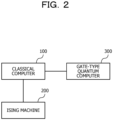
- FIG. 2 is a diagram illustrating an example of a system configuration.
- a classical computer 100 is coupled to an Ising machine 200 and a gate-type quantum computer 300.
- the classical computer 100 is, for example, a von Neumann computer.
- the Ising machine 200 is a non-von Neumann computer for calculating a ground state of an Ising model.
- the Ising machine 200 may be either one using a superconducting quantum circuit or one in which a quantum phenomenon is reproduced by a semiconductor circuit.
- the gate-type quantum computer 300 is a non-von Neumann computer that may solve a general-purpose problem by operating a quantum gate.
- the classical computer 100 controls the Ising machine 200 and the gate-type quantum computer 300 to perform quantum calculation. At that time, the classical computer 100 classifies a plurality of observables of a problem to be calculated into any one of a plurality of cliques. The classification processing into the cliques is referred to as partitioning. For example, the classical computer 100 generates an Ising model for generating a clique from information regarding a set of observables for which simultaneous measurement may be performed, and causes the Ising machine 200 to calculate a ground state of the Ising model. Then, the classical computer 100 controls the gate-type quantum computer 300 to simultaneously measure expected values of two or more observables included in the same clique.
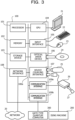
- FIG. 3 is a diagram illustrating an example of hardware of the classical computer.
- the entire device of the classical computer 100 is controlled by a processor 101.
- a memory 102 and a plurality of peripheral devices are coupled to the processor 101 via a bus 100a.
- the processor 101 may be a multiprocessor.
- the processor 101 is, for example, a central processing unit (CPU), a micro processing unit (MPU), or a digital signal processor (DSP).
- CPU central processing unit
- MPU micro processing unit
- DSP digital signal processor
- At least a part of functions implemented by the processor 101 executing a program may be implemented by an electronic circuit such as an application specific integrated circuit (ASIC) or a programmable logic device (PLD).
- ASIC application specific integrated circuit
- PLD programmable logic device
- the memory 102 is used as a main storage device of the classical computer 100.
- the memory 102 at least a part of an operating system (OS) program and an application program to be executed by the processor 101 is temporarily stored.
- OS operating system
- the memory 102 various types of data to be used in processing by the processor 101 are stored.
- a volatile semiconductor storage device such as a random access memory (RAM) is used.
- peripheral devices coupled to the bus 100a include a storage device 103, a graphics processing unit (GPU) 104, an input interface 105, an optical drive device 106, a device coupling interface 107, a network interface 108, and communication interfaces 109a and 109b.
- GPU graphics processing unit
- the storage device 103 electrically or magnetically writes and reads data to and from a built-in recording medium.
- the storage device 103 is used as an auxiliary storage device of the computer.
- an OS program, an application program, and various types of data are stored.
- a hard disk drive (HDD) or a solid state drive (SSD) may be used as the storage device 103.
- the GPU 104 is an arithmetic device that performs image processing, and is also referred to as a graphic controller.
- a monitor 21 is coupled to the GPU 104.
- the GPU 104 causes a screen of the monitor 21 to display an image according to an instruction from the processor 101.
- Examples of the monitor 21 include a display device using an organic electro luminescence (EL), a liquid crystal display device, and the like.
- a keyboard 22 and a mouse 23 are coupled to the input interface 105.
- the input interface 105 transmits signals sent from the keyboard 22 and the mouse 23 to the processor 101.
- the mouse 23 is an example of a pointing device, and another pointing device may also be used. Examples of the another pointing device include a touch panel, a tablet, a touch pad, a track ball, and the like.
- the optical drive device 106 uses laser light or the like, to read data recorded in an optical disk 24, or write data into the optical disk 24.
- the optical disk 24 is a portable recording medium in which data is recorded in a readable manner by reflection of light. Examples of the optical disk 24 include a digital versatile disc (DVD), a DVD-RAM, a compact disc read only memory (CD-ROM), a CD-recordable (R)/rewritable (RW), and the like.
- the device coupling interface 107 is a communication interface for coupling the peripheral devices to the classical computer 100.
- a memory device 25 and a memory reader/writer 26 may be coupled to the device coupling interface 107.
- the memory device 25 is a recording medium equipped with a communication function with the device coupling interface 107.
- the memory reader/writer 26 is a device that writes data to a memory card 27 or reads data from the memory card 27.
- the memory card 27 is a card-type recording medium.
- the network interface 108 is coupled to a network 20.
- the network interface 108 is coupled to another computer (including a terminal) (not illustrated) via the network 20.
- the communication interface 109a is coupled to the Ising machine 200.
- the communication interface 109a communicates with the Ising machine 200.
- the communication interface 109a transmits a search instruction for a ground state of an Ising model to the Ising machine 200.
- the communication interface 109a acquires a search result from the Ising machine 200.
- the communication interface 109b is coupled to the gate-type quantum computer 300.
- the communication interface 109b communicates with the gate-type quantum computer 300.
- the communication interface 109b instructs the gate-type quantum computer 300 to measure expected values of observables.
- the communication interface 109b acquires a measurement result of the expected values from the gate-type quantum computer 300.
- the classical computer 100 may implement processing functions of the second embodiment with the hardware as described above. Note that the information processing device 10 indicated in the first embodiment may be implemented with hardware similar to that of the classical computer 100 illustrated in FIG. 3 .
- the classical computer 100 implements the processing functions of the second embodiment by, for example, executing a program recorded in a computer-readable recording medium.
- the program in which processing content to be executed by the classical computer 100 is described may be recorded in various recording media.
- the program to be executed by the classical computer 100 may be stored in the storage device 103.
- the processor 101 loads at least a part of the program in the storage device 103 into the memory 102, and executes the program.
- the program to be executed by the classical computer 100 may also be recorded in a portable recording medium such as the optical disk 24, the memory device 25, or the memory card 27.
- the program stored in the portable recording medium may be executed after being installed in the storage device 103 under control of the processor 101, for example.
- the processor 101 may also read the program directly from the portable recording medium to execute the program.
- a quantum state may be represented using a density operator ⁇ .
- ⁇ may be represented as a 2 n ⁇ 2 n matrix (n is the number of qubits).
- the density operator ⁇ may be represented using a plurality of observables (64 in the case of three qubits). Each observable is a linearly independent basis constituting ⁇ indicating the quantum state.
- ⁇ in the case of three qubits is represented by the following expression.
- ⁇ ⁇ 0 I 0 I 1 I 2 + ⁇ 1 X 0 I 1 I 2 + ⁇ 2 Y 0 I 1 I 2 + ⁇ 3 Z 0 I 1 I 0 + ⁇ 4 I 0 X 1 I 2 + ⁇ 5 X 0 X 1 I 2 + ... + ⁇ 62 y 0 Z 1 Z 2 + ⁇ 63 Z 0 Z 1 Z 2 ⁇ 0 , ..., ⁇ 63 are coefficients of real numbers.
- X, Y, and Z with subscripts are Pauli operators, and are 2 ⁇ 2 Pauli matrices ( ⁇ x , ⁇ y , ⁇ z ). Numerical values of the subscripts are numbers of qubits to be measured.
- I with a subscript is an identity operator, and is a 2 ⁇ 2 identity matrix. The identity operator is also a type of the Pauli operator.
- the observable is represented by an array of Pauli operators. This array of the Pauli operators is referred to as a Pauli string.
- the Pauli string indicates a tensor product of the Pauli operators represented by the Pauli string.
- An expected value of an observable for a k-th term (k is a natural number) is ⁇ k .
- an expected value of X 0 X 1 I 2 is ⁇ 5 .
- ⁇ 0 is always 1, it is not needed to measure the expected value.
- the number of observables to be measured to completely know states of n qubits is 4 n -1.
- n 1, a state of a qubit may be completely known by measuring three: ⁇ X, Y, Z ⁇ observables.
- n 2
- the number of observables for which expected values are measured is 15: ⁇ I 0 X 1 , I 0 Y 1 , I 0 Z 1 , X 0 I 1 , X 0 X 1 , X 0 Y 1 , X 0 Z 1 , Y 0 I 1 , Y 0 X 1 , Y 0 Y 1 , Y 0 Z 1 , ... ⁇ .
- a plurality of observables may be simultaneously measured by a gate operation before the measurement.
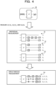
- FIG. 4 is a diagram for describing the method for simultaneously measuring observables.
- ⁇ > of three qubits is obtained. It is assumed that three observables "I 0 Y 1 X 2 , Z 0 Z 1 Z 2 , and X 0 I 1 X 2 " of a quantum circuit 30 corresponding to a problem to be solved are measured. Horizontal lines of the quantum circuit 30 correspond to the qubits.
- quantum circuits 31 to 33 corresponding to the respective three observables are generated. Rectangular symbols indicated at the horizontal lines of the quantum circuits 31 to 33 are quantum gates to be acted on the respective qubits.
- the rectangle of "S” indicates an S gate.
- the rectangle of "X” indicates an X gate.
- the rectangle of "H” indicates an H gate (Hadamard gate). At a position where a measurement symbol of each qubit is indicated, a state of the corresponding qubit is measured.
- expected values of "I 0 ", "Y 1 ", and "X 2 " are measured using three qubits.
- "I 0 " corresponding to a 0th qubit is an identity operator, and measurement of the expected value is unnecessary.
- the S gate, the H gate, and the X gate are operated.
- the expected value of Y 1 may be measured from the first qubit.
- the H gate is operated.
- the expected value of X 2 may be measured from the second qubit. Based on these measurement results, the expected value of the observable "I 0 Y 1 X 2 " may be obtained.
- expected values of "X 0 ", "I 1 ", and "X 2 " are measured using three qubits.
- "I 1 " corresponding to a first qubit is an identity operator, and measurement thereof is unnecessary.
- the H gate is operated.
- the expected value of X 0 may be measured from the 0th qubit.
- the H gate is operated.
- the expected value of X 2 may be measured from the second qubit. Based on these measurement results, the expected value of the observable "X 0 I 1 X 2 " may be obtained.
- quantum circuit 33 in order to calculate an expected value of the observable "Z 0 Z 1 Z 2 ", expected values of "Z 0 ", “Z 1 ", and “Z 2 " are measured using three qubits.
- an operation by a quantum gate on a side of output of the original quantum circuit 30 is not performed, and the expected values of "Z 0 ", “Z 1 ", and “Z 2 " may be measured by measuring the respective 0th to second qubits. Based on these measurement results, the expected value of the observable "Z 0 Z 1 Z 2 " may be obtained.
- the expected value of one observable is obtained based on the measurement results of the three qubits. Therefore, in order to obtain the expected values of the three observables, the states of the respective qubits are measured by the three quantum circuits 31 to 33.
- the H gate is provided for a 0th qubit, and a CNOT gate having a first qubit as a control bit and a second qubit as a target bit is provided.
- a SWAP gate of the 0th qubit and the first qubit is provided.
- the S gate is provided for the 0th qubit, and a CZ gate having the first qubit as the control bit and the second qubit as the target bit is provided.
- the H gate is provided for each qubit.
- the expected value of the observable "I 0 Y 1 X 2 " is obtained.
- the expected value of the observable "Z 0 Z 1 Z 2 " is obtained.
- the expected value of the observable "X 0 I 1 X 2 " is obtained.
- the expected value of one observable may be measured from one qubit, and the expected values of the three observables may be simultaneously measured. In this manner, the three observables individually measured using the quantum circuits 31 to 33 may be simultaneously measured by the one quantum circuit 34.
- FIG. 5 is a diagram illustrating a determination example of the commutation relation.
- a commutative/anticommutative correspondence table 35 whether each combination of operators is commutative or anticommutative is indicated.
- a symbol "+" indicates that operators are commutative
- a symbol "-" indicates that operators are anticommutative.
- values do not change even when multiplication order is switched, but in the case of anticommutative, signs are reversed when the multiplication order is switched.
- cliques are generated such that observables are commutative in all combinations between observables belonging to the same clique.
- FIG. 6 is a diagram illustrating an example of the partitioning. For example, for 14 observables 41 to 54, commutation relations with other observables are determined. In the example of FIG. 6 , a set of observables having a commutative commutation relation is coupled by a line. Then, cliques 61 and 62 are generated based on the commutation relations among the observables. The commutation relation becomes commutative in all combinations of observables belonging to the clique 61. Similarly, the commutation relation becomes commutative in all combinations of observables belonging to the clique 62.
- the two cliques 61 and 62 are generated, but the number of cliques to be generated changes depending on a partitioning algorithm.
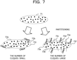
- FIG. 7 is a diagram illustrating an example of the partitioning.
- each clique of an observable group 71 is classified into any one of a plurality of cliques, there is a plurality of ways of dividing the clique. For example, it is possible to divide into three cliques 72a to 72c. Furthermore, it is also possible to divide into six cliques 73a to 73f.
- partitioning of an observable group is performed so that the number of cliques becomes smaller.
- the classical computer 100 implements the partitioning in a short time by using the Ising machine 200.
- FIG. 8 is a block diagram illustrating an example of functions of the classical computer.
- the classical computer 100 includes a commutation relation determination unit 110, a partitioning unit 120, a quantum circuit generation unit 130, an expected value acquisition unit 140, and a storage unit 150.
- the commutation relation determination unit 110 determines a commutation relation for all combinations of observables to be measured.
- the partitioning unit 120 performs partitioning on an observable group based on the commutation relations among the observables.
- the partitioning unit 120 performs the partitioning using, for example, the Ising machine 200.
- the partitioning unit 120 creates an Ising model in which energy decreases as the number of observables included in a clique increases.
- the partitioning unit 120 instructs the Ising machine 200 to search for a ground state of the created Ising model.
- information regarding the observables belonging to the clique is responded from the Ising machine 200.
- the quantum circuit generation unit 130 generates a quantum circuit for measuring observables. For example, the quantum circuit generation unit 130 selects a predetermined number of observables for simultaneous measurement from the same clique, and generates a quantum circuit corresponding to a combination of the selected observables.
- the expected value acquisition unit 140 controls the gate-type quantum computer 300 to measure the observables using the generated quantum circuit.
- the storage unit 150 stores a clique generation processing end condition 151 indicating an end condition of repeated processing for generating one clique. A clique that has been generated when the clique generation processing end condition 151 is satisfied is confirmed as a clique to be output as a result of the partitioning.
- each element of the classical computer 100 illustrated in FIG. 8 may be implemented by, for example, causing the computer to execute a program module corresponding to the element.
- FIG. 9 is a diagram illustrating an example of processing performed by the commutation relation determination unit.
- the commutation relation determination unit 110 lists observables that are elements of an observable group 40 to be measured.
- the observable is represented by a Pauli string (tensor product of Pauli operators).
- the commutation relation determination unit 110 determines a commutation relation for all pairs obtained by selecting two observables from the observable groups 40.
- the commutation relation determination unit 110 stores information associating a pair of observables determined to be commutative.
- the pair of observables determined to be commutative is coupled by a line.
- the commutation relation between observables not coupled by the line is anticommutative.
- FIG. 10 is a diagram illustrating an example of the clique generation processing.
- ⁇ i ⁇ is a binary variable.
- the partitioning unit 120 generates an Ising model 81 using ⁇ i ⁇ .
- f( ⁇ i ⁇ ) corresponds to a Hamiltonian.
- ⁇ c ij ⁇ is a non-negative constant representing a commutation relation.
- c ij 0 is satisfied.
- c ij m (m is a positive real number) is satisfied.
- a lower limit of m changes depending on the number of object observables. For example, in a case where the number of observables is about 10, the lower limit of m is about "0.25". When the number of observables is about "5000", m may be lowered to about "0.05".
- the value of m is increased, a solution is quickly converged in a solution search, but when m is excessively increased, there is a possibility that it becomes not possible to escape from a local solution in the solution search of the Ising model 81. Therefore, in a case where priority is given to calculation accuracy, it is appropriate to set the value of m to a value close to a lower limit value.
- the second term on the right side has a higher value as the number of pairs of observables in an anticommutation relation included in an element of a clique increases.
- f( ⁇ i ⁇ ) takes a minimum value in Expression (1) of the Ising model 81, the second term on the right side is needed to be 0.
- the partitioning unit 120 causes the Ising machine 200 to calculate ⁇ i ⁇ that minimizes f( ⁇ i ⁇ ).
- Expression (1) is a combinatorial optimization problem that obtains a combination of values of ⁇ i ⁇ that minimizes f( ⁇ i ⁇ ), and may be calculated at high speed by using the Ising machine 200.
- the partitioning unit 120 may increase the value of m and cause the Ising machine 200 to perform recalculation.
- the partitioning unit 120 After creating one clique from an observable group A 0 , the partitioning unit 120 sets a subgroup constituting the created clique as B 0 .
- the partitioning unit 120 repeatedly executes the clique creation processing on a subgroup having observables included in none of cliques as elements.
- FIG. 11 is a diagram illustrating an example of repeated processing of the clique generation.
- the Ising machine 200 is caused to generate the clique 61 having the maximum number of elements based on the Ising model 81.
- From the Ising machine 200 for example, ⁇ 1 , ..., ⁇ 14 ⁇ for minimizing f( ⁇ x i ⁇ ) of the Ising model 81 is responded.
- An observable corresponding to an element having a value of 1 in the responded ⁇ 1 , ..., ⁇ 14 ⁇ is an observable included in the clique 61.
- the partitioning unit 120 instructs the Ising machine 200 to generate a clique based on a subgroup having observables not included in the clique 61 as elements.
- the Ising machine 200 generates the clique 62 having the maximum number of elements according to the instruction from the partitioning unit 120.
- the quantum circuit generation unit 130 When the partitioning is ended, the quantum circuit generation unit 130 generates a quantum circuit for measuring a complete state of a qubit. Then, the expected value acquisition unit 140 controls the gate-type quantum computer 300 to acquire expected values of the observables based on the generated quantum circuit.
- FIG. 12 is a diagram illustrating an example of measurement of expected values of observables using a quantum circuit for simultaneous measurement.
- the quantum circuit generation unit 130 extracts elements corresponding to observables for simultaneous measurement from one clique of a plurality of cliques 82a, 82b, ....
- the gate-type quantum computer 300 may perform simultaneous measurement with four qubits.
- the quantum circuit generation unit 130 extracts a set of four elements from each clique.
- the quantum circuit generation unit 130 generates a quantum circuit for each combination of the extracted elements. For example, in a case where "YYXX, YXXY, XYYX, XXYY" is extracted, a quantum circuit 83 is generated.
- the generated quantum circuit 83 has a configuration in which a measurement quantum circuit 83b that performs an operation for simultaneous measurement of a plurality of observables is added to a side of output of a partial quantum circuit (unitary gate) 83a that performs an operation according to a problem to be solved.
- the measurement quantum circuit 83b is registered in advance in the quantum circuit generation unit 130 in association with, for example, a combination of observables to be measured.
- the quantum circuit generation unit 130 stores, in association with a combination pattern of observables, a quantum circuit for simultaneously measuring expected values of the observables indicated in the combination pattern.
- the quantum circuit generation unit 130 extracts, from a quantum circuit group registered in advance, a quantum circuit corresponding to the combination of the observables indicated by the elements extracted from the clique.
- the quantum circuit generation unit 130 couples the measurement quantum circuit 83b corresponding to the combination of the observables to the side of output of the partial quantum circuit 83a corresponding to the problem to be solved, and generates the quantum circuit 83 to be input to the gate-type quantum computer 300.
- the expected value acquisition unit 140 transmits the quantum circuit generated for each combination of the observables to the gate-type quantum computer 300.
- the gate-type quantum computer 300 measures expected values of the observables according to the received quantum circuit. For example, the gate-type quantum computer 300 repeats measurement of states of the respective qubits using the received quantum circuit a plurality of times. Then, the gate-type quantum computer 300 calculates the expected values of the corresponding observables based on measurement results of the plurality of times of measurement of the states of the respective qubits.
- the gate-type quantum computer 300 transmits input measurement results 84a, 84b, ... for the respective quantum circuits to the classical computer 100.
- the measurement results 84a, 84b, ... indicate the expected values of the states of the respective qubits of the corresponding quantum circuit (expected values of the observables corresponding to the corresponding qubits).
- the expected value acquisition unit 140 uses the expected values of the qubits indicated in the measurement results 84a, 84b, ... as expected values of the observables corresponding to the corresponding qubits of the quantum circuit used for calculation.
- the density operator ⁇ indicating complete states (states of an X axis, a Y axis, and a Z axis) of the output of the partial quantum circuit 83a corresponding to the problem to be solved is obtained. Then, the expected value acquisition unit 140 outputs a solution of the problem to be solved obtained based on the density operator ⁇ as a calculation result.
- a clique including as many observables as possible is repeatedly generated based on observables included in none of cliques.
- the number of cliques to be generated may be reduced.
- the clique may be created at high speed using the Ising machine 200.
- FIG. 13 is a diagram illustrating a comparison result of the number of cliques for each partitioning scheme.
- a graph 91 of FIG. 13 represents a relation between the number of observables and the number of cliques for each partitioning scheme.
- a horizontal axis represents the number of observables
- a vertical axis represents the number of cliques.
- BronK QWC “BronK QWC”, “BoppanaH QWC”, “BoppanaH GC”, and “OpenF QWC” are calculation schemes that perform partitioning without using an Ising model.
- BronK and “BoppanaH” are abbreviations for a Bron-Kerbosch algorithm and a Boppana-Halldorsson algorithm, respectively.
- OpenF is an abbreviation for a scheme using Open Fermion which is a package of PYTHON (registered trademark).
- Qubit-wise commutation (QWC) has a condition that all are commutative in comparison of sets of elements (for example, I 0 Z 0 , Y 1 Z 1 , and X 2 Z 2 in FIG.
- GC general commutation
- “Naive” i is with a dieresis
- “Naive” is a line representing the number of cliques in a case where one observable is one clique (case where the number of cliques is maximum).
- GC using Ising model (Full-tomography) and “GC using Ising model (VQE-observable)” are partitioning schemes by the partitioning unit 120 indicated in the second embodiment.
- Full-tomography in “GC using Ising model” is an example of a case where measurement of all observables for completely knowing a quantum state is performed.
- VQE-observable is an example of a case where partitioning is performed on observables used for calculation of a variational quantum eigensolver (VQE).
- "BoppanaH GC” may reduce the number of cliques to the minimum.
- the number of cliques may be about half the number of cliques of "BoppanaH GC" when compared with the same number of observables.
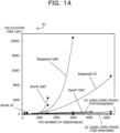
- FIG. 14 is a diagram illustrating a comparison result of a calculation time for each partitioning scheme.
- a graph 92 of FIG. 14 represents a relation between the number of observables and the calculation time for each partitioning scheme.
- a horizontal axis represents the number of observables
- a vertical axis represents the calculation time needed for partitioning.
- the Ising model by performing partitioning using the Ising model, it is possible to perform the partitioning into the small number of cliques and to shorten the calculation time.
- the above description is based on a premise that the number of observables in an observable group at the time of generating one clique from the observable group is equal to or less than the number of bits that may be used in the Ising machine 200. In a case where the number of observables in the observable group exceeds the number of bits that may be used in the Ising machine 200, it is difficult for the Ising machine 200 to perform a solution search of the Ising model for all the observables.
- an upper limit of the number of observables that may be handled in one time of the clique generation processing is the number of bits that may be used in the Ising machine 200.
- the Ising machine 200 in the case of an observable group having a scale equal to or larger than the number of bits of the Ising machine 200, the Ising machine 200 is controlled to execute the clique generation processing from a subgroup a plurality of times, thereby generating one clique.
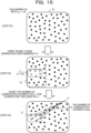
- FIG. 15 is a diagram (part 1) illustrating an example of a partitioning method for performing the plurality of times of the clique generation processing in generation of one clique.
- an observable group O to be subjected to partitioning is input (step S1).
- the observable group O is set as a subgroup O 1 used to generate a first clique.
- n bit is a natural number
- the number of all observables to be measured is larger than the number of bits n bit .
- Each observable is an element of the subgroup O 1 .
- the partitioning unit 120 of the classical computer 100 extracts n bit elements from the subgroup O 1 , and generates a subgroup O 1 ' including the n bit elements. Then, the partitioning unit 120 performs processing (first-stage clique generation) of generating a clique C 1 ' having the maximum number of elements from the subgroup O 1 ' using the Ising machine 200 (step S2). In the example of FIG. 15 , the number of elements c 1 ' (c 1 ' is a natural number) included in the clique C 1 ' is "6".
- the partitioning unit 120 counts the number of elements m(q) in the clique C 1 ' having a commutative relation with the element q (step S3).
- the number of elements c 1 ' included in the clique C 1 ' is "6"
- the number of elements m(q) of the element q is an integer within a range of "0 to 6".
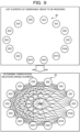
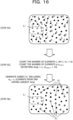
- FIG. 16 is a diagram (part 2) illustrating an example of the partitioning method for performing the plurality of times of the clique generation processing in generation of one clique.
- step S3 in FIG. 15 data indicating a value of the number of elements m(q) of each element q not included in the clique C 1 ' is generated (step S4).
- the value of the number of elements m(q) counted for the element is indicated in the vicinity of the element q not included in the clique C 1 '.
- the partitioning unit 120 arranges the elements q not included in the clique C 1 ' in descending order of the value of m(q). Then, the partitioning unit 120 generates a subset D 1 ' including the elements q from the one having the largest m(q) to n bit - c 1 -th one among the elements q (step S6). In the example of FIG. 16 , an element included in the subset D 1 ' is indicated by a double circle.
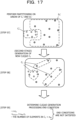
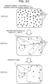
- FIG. 17 is a diagram (part 3) illustrating an example of the partitioning method for performing the plurality of times of the clique generation processing in generation of one clique.
- the partitioning unit 120 performs processing (second-stage clique generation) of generating a clique C 1 having the maximum number of elements from a union of the clique C 1 ' and the subset D 1 ' using the Ising machine 200 (step S7). As a result, the new clique C 1 is generated (step S8).
- elements surrounded by broken lines in step S8 are the elements included in the clique C 1 .
- the partitioning unit 120 determines whether or not the clique generation processing end condition 151 is satisfied (step S9).
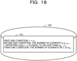
- FIG. 18 is a diagram illustrating an example of the clique generation processing end condition. In the example of FIG. 18 , three end conditions are indicated in the clique generation processing end condition 151.
- a first end condition is a condition for the maximum number of times of repetition r 0 .
- the first end condition is satisfied.
- the maximum number of times of repetition r 0 is set to a value of equal to or larger than 2 (for example, a value of about 10).
- a third end condition is that the number of elements included in a clique C i is equal to the number of bits n bit of the Ising machine 200.
- a maximum value of the number of elements included in the clique is n bit . Therefore, in a case where the number of elements included in the clique C i is equal to the number of bits n bit , the number of elements included in the clique C i does not increase even when the clique generation processing is continuously repeated more. In that case, the third end condition is satisfied.
- the partitioning unit 120 determines that the end condition of the clique generation processing is satisfied.
- the partitioning unit 120 determines that none of the end conditions is satisfied and the clique generation processing end condition 151 is not satisfied.
- FIG. 19 is a diagram (part 4) illustrating an example of the partitioning method for performing the plurality of times of the clique generation processing in generation of one clique.
- the partitioning unit 120 updates the elements of the clique C 1 ' with the elements of the clique C 1 (step S10).
- the elements of the clique C 1 ' are replaced with the elements of the clique C 1 .
- the number of elements c 1 ' included in the clique C 1 ' is "9".
- the partitioning unit 120 counts the number of elements m(q) in the clique C 1 ' having a commutative relation with the element q (step S11).
- the number of elements c 1 ' included in the clique C 1 ' is "9"
- the number of elements m(q) of the element q is an integer within a range of "0 to 9”.
- the value of the number of elements m(q) counted for the element is indicated in the vicinity of the element q not included in the clique C 1 '.
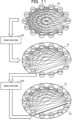
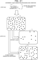
- FIG. 20 is a diagram (part 5) illustrating an example of the partitioning method for performing the plurality of times of the clique generation processing in generation of one clique.
- the partitioning unit 120 arranges the elements q not included in the clique C' in descending order of the value of m(q). Then, the partitioning unit 120 generates the subset D 1 ' including the elements q from the one having the largest m(q) to n bit - c 1 -th one among the elements q (step S13).
- an element included in the subset D 1 ' is indicated by a double circle.
- the partitioning unit 120 performs the processing (a second time of the second-stage clique generation processing) of generating the clique C 1 having the maximum number of elements from the union of the clique C 1 ' and the subset D 1 ' using the Ising machine 200 (step S14). As a result, the new clique C 1 is generated (step S15). In the example indicated in step S15, elements surrounded by broken lines are the elements included in the clique C 1 .
- FIG. 21 is a diagram (part 6) illustrating an example of the partitioning method for performing the plurality of times of the clique generation processing in generation of one clique.
- the partitioning unit 120 determines whether or not the clique generation processing end condition 151 is satisfied (step S16).
- the number of elements of C 1 is 11, and the third end condition is not satisfied.
- the partitioning unit 120 determines that the clique generation processing end condition is satisfied. Then, the partitioning unit 120 confirms the clique C 1 generated last as a clique of a partitioning result, and a subgroup O 2 obtained by excluding the elements of the clique C 1 from the subgroup O 1 is subjected to the next clique generation processing (step S17).
- the clique C 1 ' at an intermediate stage including the elements having a high possibility of being included in a clique having the maximum number of elements among the elements included in the subgroup O 1 is generated by the first-stage clique generation.
- the element q not included in the clique C 1 ' is considered to have a higher possibility of being the element included in the clique having the maximum number of elements as the number of elements m(q) in the clique C 1 ' in a commutative relation is larger. Therefore, by selecting as many elements as possible from the one having the largest number of elements m(q) as the subset D 1 ', the subset D 1 ' of the elements having a high possibility of being included in the clique having the maximum number of elements is generated. Then, by generating the clique C 1 from the union of the clique C 1 ' and the subset D 1 ', a clique having a larger number of elements may be generated.
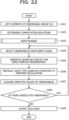
- FIG. 22 is a flowchart illustrating an example of the observable measurement procedure. Hereinafter, processing illustrated in FIG. 22 will be described in accordance with step numbers.
- the commutation relation determination unit 110 lists observables that are elements of the observable group O according to a problem to be solved. [Step S102] The commutation relation determination unit 110 determines commutation relations among the observables included as the elements in the observable group. For example, the commutation relation determination unit 110 generates all combinations (pairs of observables) obtained by selecting two observables included as the elements of the observable group.
- the commutation relation determination unit 110 determines, for each pair of observables, whether the pair of observables is commutative or anticommutative based on a relation of commutative/anticommutative between Pauli operators included in the respective observables.
- Step S103 The partitioning unit 120 performs partitioning on the observable group. By the partitioning, one or more cliques are generated. Details of the partitioning processing will be described later (see FIG. 23 ).
- the quantum circuit generation unit 130 selects, from the same clique, a predetermined number of observables for which expected values have not been calculated. [Step S105] The quantum circuit generation unit 130 generates a quantum circuit for simultaneously measuring the plurality of selected observables.
- the expected value acquisition unit 140 transmits the quantum circuit to the gate-type quantum computer 300, and instructs calculation according to the quantum circuit.
- the gate-type quantum computer 300 repeats the calculation according to the quantum circuit a predetermined number of times, and calculates an expected value of a value of a qubit corresponding to each of the selected observables.
- the gate-type quantum computer 300 transmits the obtained expected values to the expected value acquisition unit 140.
- the expected value acquisition unit 140 acquires the expected values of the observables from the gate-type quantum computer 300.
- the quantum circuit generation unit 130 determines whether or not there is an unselected observable. When there is an unselected observable, the quantum circuit generation unit 130 advances the processing to step S104. Furthermore, when all the observables have been selected, the quantum circuit generation unit 130 advances the processing to step S109.
- the expected value acquisition unit 140 obtains a solution of the problem to be solved based on the expected values of the observables to be measured, and outputs the obtained solution.
- the clique in which the observables that may be simultaneously measured are collected is generated by performing the partitioning, and the expected values of the observables included in the same clique are simultaneously measured.
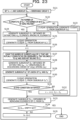
- FIG. 23 is a flowchart illustrating an example of a procedure of the partitioning processing. Hereinafter, the processing illustrated in FIG. 23 will be described in accordance with step numbers.
- Step S122 The partitioning unit 120 determines whether or not the number of elements M k of a subgroup O k is larger than the number of bits n bit of the Ising machine 200. In a case where the number of elements M k of the subgroup O k is larger, the partitioning unit 120 advances the processing to step S124. Furthermore, when the number of elements M k of the subgroup O k is equal to or less than the number of bits n bit , the partitioning unit 120 advances the processing to step S123.
- Step S123 The partitioning unit 120 generates a clique C k from the subgroup O k . Details of the clique generation processing will be described later (see FIGs. 24 and 25 ). After generating the clique C k , the partitioning unit 120 advances the processing to step S133.
- the partitioning unit 120 generates a subgroup O k ' obtained by optionally extracting n bit elements among the M k elements of the subgroup O k .
- the partitioning unit 120 generates a clique C k ' having the maximum number of elements from the subgroup O k '. It is assumed that the number of elements included in the clique C k ' is c k '.
- This processing is processing in which the subgroup O k in the clique generation processing of step S123 is replaced with the subgroup O k ', and details of the processing are as indicated in FIGs. 24 and 25 .
- Step S128 The partitioning unit 120 generates a subgroup D k ' having, as elements, n bit - C k ' observables in descending order of m(q i ) among the observables ⁇ q i ⁇ .
- Step S129 The partitioning unit 120 generates a subgroup O k " of a union of the clique C k ' and the subgroup D k '.
- Step S130 The partitioning unit 120 generates the clique C k having the maximum number of elements from the subgroup O k ".
- This processing is processing in which the subgroup O k in the clique generation processing of step S123 is replaced with the subgroup O k ", and details of the processing are as indicated in FIGs. 19 and 20 .
- Step S131 The partitioning unit 120 determines whether or not at least one of the end conditions indicated in the clique generation processing end condition 151 is satisfied. In a case where any one of the end conditions is satisfied, the partitioning unit 120 advances the processing to step S133. Furthermore, in a case where none of the end conditions is satisfied, the partitioning unit 120 advances the processing to step S132.
- Step S132 The partitioning unit 120 adds 1 to the loop variable r (r ⁇ r + 1). Furthermore, the partitioning unit 120 substitutes the clique C k generated in step S130 into the unconfirmed clique C k ' (C k ' ⁇ C k ). Then, the partitioning unit 120 advances the processing to step S127.
- Step S133 The partitioning unit 120 generates a subgroup O k+1 obtained by removing elements of the clique C k from the subgroup O k .
- Step S134 The partitioning unit 120 determines whether or not the subgroup O k+1 is an empty set. When the subgroup O k+1 is an empty set, the partitioning unit 120 ends the partitioning processing. Furthermore, when the subgroup O k+1 is not an empty set, the partitioning unit 120 advances the processing to step S135.
- Step S135 The partitioning unit 120 counts up the value of the variable k, and advances the processing to step S122 (k ⁇ k + 1).
- the generation of the clique C k is repeatedly executed until all the observables, which are the elements of the observable group O, are included in any one clique.
- the partitioning method of performing the plurality of times of the clique generation processing in generating one clique is applied.
- the clique generation processing is performed twice or more (steps S125 and S130) in generating one clique.
- FIG. 24 is a flowchart (1/2) illustrating an example of a procedure of the clique generation processing. Hereinafter, the processing illustrated in FIG. 24 will be described in accordance with step numbers.
- the partitioning unit 120 creates an Ising model of the subgroup to be subjected to the processing.
- a value of a Hamiltonian decreases as the number of observables included in a clique increases.
- Step S202 The partitioning unit 120 sets the number of observables of the subgroup to be subjected to the processing to L (L is a natural number), and sets the respective observables to ⁇ P 1 , P 2 , ..., P L ⁇ . Each observable is represented by a Pauli string.
- Step S203 The partitioning unit 120 generates an L ⁇ L square matrix E in which values of all elements are "0".
- the partitioning unit 120 counts up a loop variable n1 from 1 by 1, and repeats processing of steps S205 to S208 until the loop variable n1 becomes L.
- Step S205 The partitioning unit 120 counts up a loop variable n2 from n1 by 1, and repeats the processing of steps S206 and S207 until the loop variable n2 becomes L.
- Step S208 In a case where the processing of steps S206 and S207 is ended for all n2 from n1 to L, the partitioning unit 120 advances the processing to step S209.
- Step S209 In a case where the processing of steps S205 to S208 is ended for all n1 from 1 to L, the partitioning unit 120 advances the processing to step S211 (see FIG. 25 ).
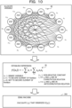
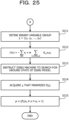
- FIG. 25 is a flowchart (2/2) illustrating an example of the procedure of the clique generation processing.
- the partitioning unit 120 generates an Ising model.
- Step S213 The partitioning unit 120 transmits the Ising model to the Ising machine 200, and instructs the Ising machine 200 to search for a ground state of the Ising model.
- the Ising machine 200 generates the binary variable group ⁇ that minimizes f( ⁇ ) in the Ising model according to the instruction.
- Step S214 The partitioning unit 120 acquires the binary variable group ⁇ that minimizes f( ⁇ ) from the Ising machine 200.
- the set P includes an observable corresponding to a variable having a value of "1" in the binary variable group ⁇ that minimizes f( ⁇ ).
- the Ising machine 200 by causing the Ising machine 200 to search for the ground state of the Ising model based on the Ising model corresponding to the subset to be subjected to the processing, it is possible to generate the clique having the maximum number of elements.
- the clique C k is generated.
- the clique C k ' is generated.
- the clique C k is generated.
- the clique generation processing is repeated a number of times equal to or less than the number of times of repetition r 0 , and then the clique C k generated in the last clique generation processing is confirmed as a result of the partitioning.
- the clique generation processing By repeatedly executing the clique generation processing, there is a high possibility that a clique including more elements may be generated. As a result, the number of cliques generated in partitioning may be reduced.
- the clique generation processing end condition since there are the second and third end conditions as the clique generation processing end condition, for example, it is possible to generate a clique including many observables with a small increase in processing amount as compared with the case of only the first end condition. Note that the effect of reducing the number of cliques by performing the clique generation a plurality of times to confirm one clique is higher as the number of bits of the Ising machine 200 is smaller.
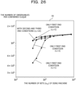
- FIG. 26 is a diagram illustrating an effect of reducing the number of cliques according to the number of bits of an Ising machine.
- a horizontal axis represents the number of bits of the Ising machine 200
- a vertical axis represents the number of observables per confirmed clique.
- the number of observables per confirmed clique is a value obtained by dividing the number of elements of the observable group to be subjected to partitioning by the number of cliques obtained as a result of the partitioning.
- the graph 93 illustrates a result of the partitioning for each number of bits of the Ising machine 200 in a case where only the first end condition is applied as the clique generation processing end condition and in a case where the second and third end conditions are also applied.
- the number of observables per confirmed clique increases. In other words, the number of cliques obtained as a result of the partitioning is reduced.
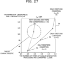
- FIG. 27 is a diagram illustrating a first example of a relation between a processing amount and the number of observables in a clique.
- a graph 94 indicates a relation between the processing amount and the number of observables in the clique in a case where the number of bits n bit of the Ising machine 200 is 384.
- a horizontal axis of the graph 94 represents the number of times of the clique generation processing per confirmed clique.
- a vertical axis of the graph 94 represents the number of observables per confirmed clique.
- Points P1, P2, and P3 in the graph 94 are examples in a case where the end condition in the clique generation processing end condition 151 is only the first end condition.
- the characteristic of the partitioning processing falls within the range of the target characteristic.
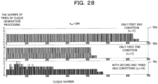
- FIG. 28 is a diagram illustrating a first example of the number of times of the clique generation processing for each confirmed clique.
- Horizontal axes of the graphs 95a to 95c represent numbers assigned to the confirmed cliques in ascending order from an earliest confirmed one. Vertical axes of the graphs 95a to 95c represent the number of times of the clique generation processing executed until each clique is confirmed.
- the number of times of the clique generation processing executed until one clique is confirmed varies.
- five times of the clique generation processing may be performed to confirm the clique, but in many cases, the clique may be confirmed by two times of the clique generation processing. Therefore, the total number of times of execution of the clique generation processing is smaller than that in a case where the second and third end conditions are not applied.
- the processing of confirming one clique by executing the clique generation processing using the Ising machine 200 a plurality of times is more effective as the number of bits of the Ising machine 200 relative to the number of elements of the observable group is smaller.
- the number of bits of the Ising machine 200 is 384 in the examples illustrated in FIGs. 27 and 28 , examples in which the number of bits is 512 are illustrated in FIGs. 29 and 30 .
- FIG. 29 is a diagram illustrating a second example of the relation between the processing amount and the number of observables in the clique.
- a graph 96 indicates a result of performing the partitioning under the same condition as in the example of FIG. 27 except that the number of bits n bit of the Ising machine 200 is 512.
- Points P5, P6, and P7 in the graph 96 are examples in a case where the end condition in the clique generation processing end condition 151 is only the first end condition.
- the second and third end conditions are added to the clique generation processing end condition 151, so that the characteristic of the partitioning becomes the target characteristic.
- the number of cliques may be greatly reduced with a small increase in a calculation amount.
- FIG. 30 is a diagram illustrating a second example of the number of times of the clique generation processing for each confirmed clique.
- Horizontal axes of the graphs 97a to 97c represent numbers assigned to the confirmed cliques in ascending order from an earliest confirmed one. Vertical axes of the graphs 97a to 97c represent the number of times of the clique generation processing executed until each clique is confirmed.
- n bit 512
- a condition that the number of elements q in which m(q) is equal to or larger than a predetermined threshold is equal to or less than n bit - c i may be applied.
- the threshold at this time is a value equal to or less than c i (for example, a value obtained by multiplying c i by 0.9).
- a condition that the number of elements of C i is equal to or larger than a predetermined threshold may be applied.
- the threshold at this time is a value equal to or less than n bit (for example, a value obtained by multiplying n bit by 0.9).
Landscapes
- Engineering & Computer Science (AREA)
- Theoretical Computer Science (AREA)
- Physics & Mathematics (AREA)
- General Physics & Mathematics (AREA)
- Computing Systems (AREA)
- Artificial Intelligence (AREA)
- Data Mining & Analysis (AREA)
- Evolutionary Computation (AREA)
- Software Systems (AREA)
- Mathematical Physics (AREA)
- General Engineering & Computer Science (AREA)
- Condensed Matter Physics & Semiconductors (AREA)
- Pure & Applied Mathematics (AREA)
- Mathematical Optimization (AREA)
- Mathematical Analysis (AREA)
- Computational Mathematics (AREA)
- Computational Linguistics (AREA)
- Management, Administration, Business Operations System, And Electronic Commerce (AREA)
- Debugging And Monitoring (AREA)
Applications Claiming Priority (1)
| Application Number | Priority Date | Filing Date | Title |
|---|---|---|---|
| PCT/JP2022/018970 WO2023209828A1 (ja) | 2022-04-26 | 2022-04-26 | 複数量子ビットオブザーバブルのパーティショニングプログラム、複数量子ビットオブザーバブルのパーティショニング方法、および情報処理装置 |
Publications (2)
| Publication Number | Publication Date |
|---|---|
| EP4517604A1 true EP4517604A1 (de) | 2025-03-05 |
| EP4517604A4 EP4517604A4 (de) | 2025-06-11 |
Family
ID=88518321
Family Applications (1)
| Application Number | Title | Priority Date | Filing Date |
|---|---|---|---|
| EP22940108.8A Pending EP4517604A4 (de) | 2022-04-26 | 2022-04-26 | Programm zur partitionierung von mehrfach-qubit-observables, verfahren zur partitionierung von mehrfach-qubit-observables und informationsverarbeitungsvorrichtung |
Country Status (4)
| Country | Link |
|---|---|
| US (1) | US20250037000A1 (de) |
| EP (1) | EP4517604A4 (de) |
| JP (1) | JP7667523B2 (de) |
| WO (1) | WO2023209828A1 (de) |
Families Citing this family (1)
| Publication number | Priority date | Publication date | Assignee | Title |
|---|---|---|---|---|
| JP2025145553A (ja) * | 2024-03-21 | 2025-10-03 | 富士通株式会社 | 情報処理プログラム、情報処理方法、および情報処理装置 |
Family Cites Families (7)
| Publication number | Priority date | Publication date | Assignee | Title |
|---|---|---|---|---|
| US11275816B2 (en) | 2019-02-25 | 2022-03-15 | International Business Machines Corporation | Selection of Pauli strings for Variational Quantum Eigensolver |
| CN113544711B (zh) | 2019-01-17 | 2024-08-02 | D-波系统公司 | 用于使用聚类收缩的混合算法系统和方法 |
| JP7125825B2 (ja) * | 2019-01-24 | 2022-08-25 | インターナショナル・ビジネス・マシーンズ・コーポレーション | エンタングルした測定を用いたパウリ文字列のグループ化 |
| US11410069B2 (en) * | 2019-04-25 | 2022-08-09 | International Business Machines Corporation | Grouping of Pauli observables using Bell measurements |
| JP7219402B2 (ja) | 2019-06-27 | 2023-02-08 | 富士通株式会社 | 最適化装置、最適化装置の制御方法及び最適化装置の制御プログラム |
| JP7417074B2 (ja) | 2020-02-19 | 2024-01-18 | 富士通株式会社 | 最適化装置、最適化方法及び最適化装置の制御プログラム |
| WO2021220445A1 (ja) | 2020-04-29 | 2021-11-04 | 株式会社日立製作所 | 演算システム、情報処理装置、および最適解探索処理方法 |
-
2022
- 2022-04-26 JP JP2024517672A patent/JP7667523B2/ja active Active
- 2022-04-26 WO PCT/JP2022/018970 patent/WO2023209828A1/ja not_active Ceased
- 2022-04-26 EP EP22940108.8A patent/EP4517604A4/de active Pending
-
2024
- 2024-09-23 US US18/892,614 patent/US20250037000A1/en active Pending
Also Published As
| Publication number | Publication date |
|---|---|
| EP4517604A4 (de) | 2025-06-11 |
| JPWO2023209828A1 (de) | 2023-11-02 |
| US20250037000A1 (en) | 2025-01-30 |
| WO2023209828A1 (ja) | 2023-11-02 |
| JP7667523B2 (ja) | 2025-04-23 |
Similar Documents
| Publication | Publication Date | Title |
|---|---|---|
| US7801836B2 (en) | Automated predictive data mining model selection using a genetic algorithm | |
| US20220335323A1 (en) | Solution system, solution method, and solution program | |
| Pappa et al. | Attribute selection with a multi-objective genetic algorithm | |
| JP7394413B2 (ja) | 量子系の固有状態の取得方法、装置、デバイス及び記憶媒体 | |
| US20260050812A1 (en) | Quantum computing method for solving combinatorial optimization problems | |
| Singh et al. | Modeling quantum machine learning for genomic data analysis | |
| Li et al. | Fast classification for large data sets via random selection clustering and support vector machines | |
| US20250037000A1 (en) | Computer-readable recording medium storing partitioning program for multi-qubit observables, partitioning method for multi-qubit observables, and information processing device | |
| JP7534701B2 (ja) | 複数量子ビットオブザーバブルのパーティショニング方法、複数量子ビットオブザーバブルのパーティショニングプログラム、および情報処理装置 | |
| CN114925843A (zh) | 基于量子退火求解最小特征问题的方法 | |
| Li et al. | Fast support vector machine classification for large data sets | |
| Gakii et al. | Feature selection for classification using WGCNA and Spread Sub-Sample for an imbalanced rheumatoid arthritis RNASEQ data | |
| Singh et al. | Genetic Algorithm based Feature Selection to Enhance Breast Cancer Classification | |
| JP7470019B2 (ja) | 情報処理システム | |
| Pontes-Filho et al. | EvoDynamic: a framework for the evolution of generally represented dynamical systems and its application to criticality | |
| JP7332874B2 (ja) | 最適化システム、最適化支援装置、最適化支援方法、および最適化支援プログラム | |
| US20260037847A1 (en) | Observable measurement support method and information processing apparatus | |
| WO2023139681A1 (ja) | 複数量子ビットオブザーバブルのパーティショニングプログラム、複数量子ビットオブザーバブルのパーティショニング方法、および情報処理装置 | |
| Tao et al. | Software defect prediction method based on clustering ensemble learning | |
| Sergienko et al. | Michigan and Pittsburgh methods combination for fuzzy classifier design with coevolutionary algorithm | |
| Jabbar et al. | Grey wolf optimization algorithm for hierarchical document clustering | |
| EP4629141A1 (de) | Erzeugungsprogramm, erzeugungsverfahren und informationsverarbeitungsvorrichtung | |
| EP4675494A1 (de) | Aktives lernprogramm, verfahren zum aktiven lernen und informationsverarbeitungsvorrichtung | |
| EP4641452A1 (de) | Quantenberechnungsunterstützungsprogramm, quantenberechnungsunterstützungsverfahren und informationsverarbeitungsvorrichtung | |
| EP4343637A1 (de) | Arithmetisches operationsprogramm, arithmetisches operationsverfahren und informationsverarbeitungsvorrichtung |
Legal Events
| Date | Code | Title | Description |
|---|---|---|---|
| STAA | Information on the status of an ep patent application or granted ep patent |
Free format text: STATUS: THE INTERNATIONAL PUBLICATION HAS BEEN MADE |
|
| PUAI | Public reference made under article 153(3) epc to a published international application that has entered the european phase |
Free format text: ORIGINAL CODE: 0009012 |
|
| STAA | Information on the status of an ep patent application or granted ep patent |
Free format text: STATUS: REQUEST FOR EXAMINATION WAS MADE |
|
| 17P | Request for examination filed |
Effective date: 20240919 |
|
| AK | Designated contracting states |
Kind code of ref document: A1 Designated state(s): AL AT BE BG CH CY CZ DE DK EE ES FI FR GB GR HR HU IE IS IT LI LT LU LV MC MK MT NL NO PL PT RO RS SE SI SK SM TR |
|
| REG | Reference to a national code |
Ref country code: DE Ref legal event code: R079 Free format text: PREVIOUS MAIN CLASS: G06N0010000000 Ipc: G06N0010600000 |
|
| A4 | Supplementary search report drawn up and despatched |
Effective date: 20250512 |
|
| RIC1 | Information provided on ipc code assigned before grant |
Ipc: G06N 10/20 20220101ALN20250506BHEP Ipc: G06N 5/01 20230101ALI20250506BHEP Ipc: G06N 10/60 20220101AFI20250506BHEP |
|
| DAV | Request for validation of the european patent (deleted) | ||
| DAX | Request for extension of the european patent (deleted) | ||
| REG | Reference to a national code |
Ref country code: DE Ref legal event code: R079 Free format text: PREVIOUS MAIN CLASS: G06N0010600000 Ipc: G06N0010200000 |
|
| GRAP | Despatch of communication of intention to grant a patent |
Free format text: ORIGINAL CODE: EPIDOSNIGR1 |
|
| STAA | Information on the status of an ep patent application or granted ep patent |
Free format text: STATUS: GRANT OF PATENT IS INTENDED |
|
| RIC1 | Information provided on ipc code assigned before grant |
Ipc: G06N 10/20 20220101AFI20260318BHEP Ipc: G06N 5/01 20230101ALI20260318BHEP |