EP4361753A2 - Planung bei mobilen robotern - Google Patents
Planung bei mobilen robotern Download PDFInfo
- Publication number
- EP4361753A2 EP4361753A2 EP24163038.3A EP24163038A EP4361753A2 EP 4361753 A2 EP4361753 A2 EP 4361753A2 EP 24163038 A EP24163038 A EP 24163038A EP 4361753 A2 EP4361753 A2 EP 4361753A2
- Authority
- EP
- European Patent Office
- Prior art keywords
- mobile robot
- trajectory
- stage
- scenario
- robot trajectory
- Prior art date
- Legal status (The legal status is an assumption and is not a legal conclusion. Google has not performed a legal analysis and makes no representation as to the accuracy of the status listed.)
- Granted
Links
Images


Classifications
-
- G—PHYSICS
- G05—CONTROLLING; REGULATING
- G05D—SYSTEMS FOR CONTROLLING OR REGULATING NON-ELECTRIC VARIABLES
- G05D1/00—Control of position, course, altitude or attitude of land, water, air or space vehicles, e.g. using automatic pilots
- G05D1/02—Control of position or course in two dimensions
- G05D1/021—Control of position or course in two dimensions specially adapted to land vehicles
- G05D1/0212—Control of position or course in two dimensions specially adapted to land vehicles with means for defining a desired trajectory
- G05D1/0217—Control of position or course in two dimensions specially adapted to land vehicles with means for defining a desired trajectory in accordance with energy consumption, time reduction or distance reduction criteria
-
- G—PHYSICS
- G05—CONTROLLING; REGULATING
- G05D—SYSTEMS FOR CONTROLLING OR REGULATING NON-ELECTRIC VARIABLES
- G05D1/00—Control of position, course, altitude or attitude of land, water, air or space vehicles, e.g. using automatic pilots
- G05D1/02—Control of position or course in two dimensions
- G05D1/021—Control of position or course in two dimensions specially adapted to land vehicles
- G05D1/0212—Control of position or course in two dimensions specially adapted to land vehicles with means for defining a desired trajectory
- G05D1/0214—Control of position or course in two dimensions specially adapted to land vehicles with means for defining a desired trajectory in accordance with safety or protection criteria, e.g. avoiding hazardous areas
-
- B—PERFORMING OPERATIONS; TRANSPORTING
- B60—VEHICLES IN GENERAL
- B60W—CONJOINT CONTROL OF VEHICLE SUB-UNITS OF DIFFERENT TYPE OR DIFFERENT FUNCTION; CONTROL SYSTEMS SPECIALLY ADAPTED FOR HYBRID VEHICLES; ROAD VEHICLE DRIVE CONTROL SYSTEMS FOR PURPOSES NOT RELATED TO THE CONTROL OF A PARTICULAR SUB-UNIT
- B60W30/00—Purposes of road vehicle drive control systems not related to the control of a particular sub-unit, e.g. of systems using conjoint control of vehicle sub-units
- B60W30/08—Active safety systems predicting or avoiding probable or impending collision or attempting to minimise its consequences
- B60W30/095—Predicting travel path or likelihood of collision
- B60W30/0956—Predicting travel path or likelihood of collision the prediction being responsive to traffic or environmental parameters
-
- B—PERFORMING OPERATIONS; TRANSPORTING
- B60—VEHICLES IN GENERAL
- B60W—CONJOINT CONTROL OF VEHICLE SUB-UNITS OF DIFFERENT TYPE OR DIFFERENT FUNCTION; CONTROL SYSTEMS SPECIALLY ADAPTED FOR HYBRID VEHICLES; ROAD VEHICLE DRIVE CONTROL SYSTEMS FOR PURPOSES NOT RELATED TO THE CONTROL OF A PARTICULAR SUB-UNIT
- B60W30/00—Purposes of road vehicle drive control systems not related to the control of a particular sub-unit, e.g. of systems using conjoint control of vehicle sub-units
- B60W30/18—Propelling the vehicle
- B60W30/18009—Propelling the vehicle related to particular drive situations
- B60W30/18159—Traversing an intersection
-
- B—PERFORMING OPERATIONS; TRANSPORTING
- B60—VEHICLES IN GENERAL
- B60W—CONJOINT CONTROL OF VEHICLE SUB-UNITS OF DIFFERENT TYPE OR DIFFERENT FUNCTION; CONTROL SYSTEMS SPECIALLY ADAPTED FOR HYBRID VEHICLES; ROAD VEHICLE DRIVE CONTROL SYSTEMS FOR PURPOSES NOT RELATED TO THE CONTROL OF A PARTICULAR SUB-UNIT
- B60W30/00—Purposes of road vehicle drive control systems not related to the control of a particular sub-unit, e.g. of systems using conjoint control of vehicle sub-units
- B60W30/18—Propelling the vehicle
- B60W30/18009—Propelling the vehicle related to particular drive situations
- B60W30/18163—Lane change; Overtaking manoeuvres
-
- B—PERFORMING OPERATIONS; TRANSPORTING
- B60—VEHICLES IN GENERAL
- B60W—CONJOINT CONTROL OF VEHICLE SUB-UNITS OF DIFFERENT TYPE OR DIFFERENT FUNCTION; CONTROL SYSTEMS SPECIALLY ADAPTED FOR HYBRID VEHICLES; ROAD VEHICLE DRIVE CONTROL SYSTEMS FOR PURPOSES NOT RELATED TO THE CONTROL OF A PARTICULAR SUB-UNIT
- B60W60/00—Drive control systems specially adapted for autonomous road vehicles
- B60W60/001—Planning or execution of driving tasks
- B60W60/0011—Planning or execution of driving tasks involving control alternatives for a single driving scenario, e.g. planning several paths to avoid obstacles
-
- G—PHYSICS
- G01—MEASURING; TESTING
- G01C—MEASURING DISTANCES, LEVELS OR BEARINGS; SURVEYING; NAVIGATION; GYROSCOPIC INSTRUMENTS; PHOTOGRAMMETRY OR VIDEOGRAMMETRY
- G01C21/00—Navigation; Navigational instruments not provided for in groups G01C1/00 - G01C19/00
- G01C21/26—Navigation; Navigational instruments not provided for in groups G01C1/00 - G01C19/00 specially adapted for navigation in a road network
- G01C21/34—Route searching; Route guidance
- G01C21/3407—Route searching; Route guidance specially adapted for specific applications
-
- G—PHYSICS
- G05—CONTROLLING; REGULATING
- G05D—SYSTEMS FOR CONTROLLING OR REGULATING NON-ELECTRIC VARIABLES
- G05D1/00—Control of position, course, altitude or attitude of land, water, air or space vehicles, e.g. using automatic pilots
- G05D1/0088—Control of position, course, altitude or attitude of land, water, air or space vehicles, e.g. using automatic pilots characterized by the autonomous decision making process, e.g. artificial intelligence, predefined behaviours
-
- G—PHYSICS
- G05—CONTROLLING; REGULATING
- G05D—SYSTEMS FOR CONTROLLING OR REGULATING NON-ELECTRIC VARIABLES
- G05D1/00—Control of position, course, altitude or attitude of land, water, air or space vehicles, e.g. using automatic pilots
- G05D1/02—Control of position or course in two dimensions
- G05D1/021—Control of position or course in two dimensions specially adapted to land vehicles
- G05D1/0212—Control of position or course in two dimensions specially adapted to land vehicles with means for defining a desired trajectory
- G05D1/0221—Control of position or course in two dimensions specially adapted to land vehicles with means for defining a desired trajectory involving a learning process
-
- G—PHYSICS
- G05—CONTROLLING; REGULATING
- G05D—SYSTEMS FOR CONTROLLING OR REGULATING NON-ELECTRIC VARIABLES
- G05D1/00—Control of position, course, altitude or attitude of land, water, air or space vehicles, e.g. using automatic pilots
- G05D1/02—Control of position or course in two dimensions
- G05D1/021—Control of position or course in two dimensions specially adapted to land vehicles
- G05D1/0231—Control of position or course in two dimensions specially adapted to land vehicles using optical position detecting means
- G05D1/0238—Control of position or course in two dimensions specially adapted to land vehicles using optical position detecting means using obstacle or wall sensors
-
- G—PHYSICS
- G05—CONTROLLING; REGULATING
- G05D—SYSTEMS FOR CONTROLLING OR REGULATING NON-ELECTRIC VARIABLES
- G05D1/00—Control of position, course, altitude or attitude of land, water, air or space vehicles, e.g. using automatic pilots
- G05D1/02—Control of position or course in two dimensions
- G05D1/021—Control of position or course in two dimensions specially adapted to land vehicles
- G05D1/0231—Control of position or course in two dimensions specially adapted to land vehicles using optical position detecting means
- G05D1/0246—Control of position or course in two dimensions specially adapted to land vehicles using optical position detecting means using a video camera in combination with image processing means
-
- G—PHYSICS
- G05—CONTROLLING; REGULATING
- G05D—SYSTEMS FOR CONTROLLING OR REGULATING NON-ELECTRIC VARIABLES
- G05D1/00—Control of position, course, altitude or attitude of land, water, air or space vehicles, e.g. using automatic pilots
- G05D1/60—Intended control result
- G05D1/644—Optimisation of travel parameters, e.g. of energy consumption, journey time or distance
-
- B—PERFORMING OPERATIONS; TRANSPORTING
- B60—VEHICLES IN GENERAL
- B60W—CONJOINT CONTROL OF VEHICLE SUB-UNITS OF DIFFERENT TYPE OR DIFFERENT FUNCTION; CONTROL SYSTEMS SPECIALLY ADAPTED FOR HYBRID VEHICLES; ROAD VEHICLE DRIVE CONTROL SYSTEMS FOR PURPOSES NOT RELATED TO THE CONTROL OF A PARTICULAR SUB-UNIT
- B60W2420/00—Indexing codes relating to the type of sensors based on the principle of their operation
- B60W2420/40—Photo, light or radio wave sensitive means, e.g. infrared sensors
- B60W2420/403—Image sensing, e.g. optical camera
Definitions
- the present invention pertains to planning in autonomous vehicles and other mobile robots.
- An autonomous vehicle also known as a self-driving vehicle, refers to a vehicle which has a sensor system for monitoring its external environment and a control system that is capable of making and implementing driving decisions automatically using those sensors. This includes in particular the ability to automatically adapt the vehicle's speed and direction of travel based on perception inputs from the sensor system.
- a fully-autonomous or "driverless" vehicle has sufficient decision-making capability to operate without any input from a human driver.
- autonomous vehicle as used herein also applies to semi-autonomous vehicles, which have more limited autonomous decision-making capability and therefore still require a degree of oversight from a human driver.
- Other mobile robots are being developed, for example for carrying freight supplies in internal and external industrial zones. Such mobile robots would have no people on board and belong to a class of mobile robot termed UAV (unmanned autonomous vehicle).
- UAV unmanned autonomous vehicle
- Autonomous air mobile robots (drones) are also being developed.
- a receding horizon planner is formulated as Nonlinear Model Predictive Control (NMPC), subject to a set of hard constraints, namely (1) respecting a transition model of the system, including kinematic and dynamic constraints (2) maintaining the vehicle within the limits of the road and (3) avoiding other traffic participants in the sense of guaranteeing a probability of collision below p ⁇ .
- NMPC Nonlinear Model Predictive Control
- a cost function penalizes deviation from a current acceleration and steering angle specified by a human driver - a form of "soft constraint" or "objective” according to the terminology used herein.
- [C-1] formulate planning as a non-linear constrained optimization problem, and seek to solve that problem using a receding horizon formulation (the solution being a set of control inputs that optimize the cost function). It is possible to extend this framework to more complex cost functions, for example with explicit comfort objectives, or to include more sophisticated vehicle (or, more generally, mobile robot) models.
- a challenge with this approach is that convergence to an optimal set of control inputs is both slow and uncertain, particularly as the complexity of the cost function and/or the mobile robot model increases, i.e. the optimizer may take a long time to converge to a solution, or may never successfully converge.
- Another challenge is that non-linear constrained optimization solvers tend to be local in nature and thus have a tendency to converge to local optima which may be far from the globally optimal solution. This can significantly impact mobile robot performance.
- the present invention also formulates mobile robot planning as a constrained optimization problem. Given a scenario with a desired goal, the problem is to find a series of control actions (“policy") that substantially (exactly or approximately) globally optimises a defined cost function for the scenario and the desired goal.
- policy a series of control actions
- a core issue addressed herein is speed of convergence in constrained optimization trajectory planning, i.e. for planners that formulate trajectory planning (synthesis) as a constrained optimization subject to a set of hard constraints.
- constrained optimization-based planners that can not only provide highly quality trajectories but also converge to an acceptable solution (trajectory) in real-time is challenging using current hardware and state of the art solvers.
- hard constraints are constraints that a planned trajectory must be guaranteed to satisfy. These could, for example, be constraints on collision avoidance (avoiding collisions with static or moving obstacles), permitted area constraints (e.g. constraining planned trajectories to keep within a road layout or other permitted area), or comfort constraints for autonomous vehicles.
- One aspect herein provides a computer system for planning mobile robot trajectories, the computer system comprising: an input configured to receive a set of scenario description parameters describing a scenario and a desired goal for the mobile robot therein; a runtime optimizer configured to compute a final mobile robot trajectory that substantially optimizes a cost function for the scenario, subject to a set of hard constraints that the final mobile robot trajectory is guaranteed to satisfy; and a trained function approximator configured to compute, from the set of scenario description parameters, initialization data defining an initial mobile robot trajectory; wherein the computer system is configured to initialize the runtime optimizer with the initialization data, in order to guide the optimizer from the initial mobile robot trajectory to the final mobile robot trajectory that satisfies the hard constraints, the function approximator having been trained on example sets of scenario description parameters and ground truth initialization data for the example sets of scenario description parameters.
- the function approximator may, for example, take the form of a neural network. Function approximators may require significant amounts of data to train, and therefore require significant resources in training. However, once trained, a function approximator is efficient to implement, and can be applied to scenarios in order to generate initialization data quickly, even on resource-constrained platforms.
- the initialization data provides a starting point for the search by the optimizer for a globally optimal solution (the final trajectory). It could, for example, take the form of an initial trajectory and/or an initial sequence of control actions that define the initial vehicle trajectory in conjunction with an ego dynamics model(s) (or some other initialization data derived from one of both of those).
- the initial trajectory is not necessarily guaranteed to satisfy any hard constraints (even if such constrains have been imposed during training - see below). However, this is not an issue, because the initial trajectory is only used to initialize the runtime optimizer. The final trajectory determined by the runtime optimizer is guaranteed to satisfy the hard constraints.
- the present disclosure addresses local optima problems that arise in the context of planning based on constrained optimization.
- the full constrained optimization problem to be solved is non-linear.
- the runtime planner may therefore take the form of a constrained non-linear optimizer.
- Non-linear optimizers are particularly vulnerable to convergence to locally but non-globally optimal solutions.
- a high-quality initialization that is reasonably close to the global optima can significantly instances of convergence to non-local optima.
- the training data used to train the function approximator may also be generated using a constrained optimization-based planner, i.e. the function approximator may be trained to approximate (imitate) a constrained non-linear optimization.
- the function approximator may be trained to a multi-stage constrained optimisation planner, in which a first stage is formulated as an optimization problem that is similar to, but simpler than a more complex planning problem that ultimately needs to be solved.
- the first stage may use a linear cost function and linear robot dynamics model. Such a problem is generally less susceptible to local optima.
- the solution of the first stage is then used to initialize the second stage, in which the "full" planning problem is solved.
- the solution of the first stage will be more likely to be close to a globally optimal solution to the full planning problem - up to up to some acceptable level of error introduced by the simplification assumptions of the first stage - and therefore reduces the tendency of the second stage to converge to local optima far from the global solution.
- the first and second optimization stages form part of a planner that the function approximator is trained to imitate - referred to herein as a "reference” or “expert” planner. Those stages do not need to be implemented at runtime, because the trained function approximator is implemented at runtime instead.
- the expert planner is therefore not required to be able to operate in real-time in order to achieve real-time operation at runtime.
- the runtime optimizer is separate from both of the above constrained optimization stages - although, in some embodiments, it may implement the same or similar logic to the second stage of the multi-stage planner. In contrast to the multi-stage planner, the runtime optimizer is implemented at runtime. Because the runtime optimizer is provided with a high-quality initialization from the trained function approximator, it is significantly less likely to converge to local optima, and can also complete its search for the final mobile robot trajectory in real time.
- the function approximator may have been trained to approximate a reference planner, the ground truth initialization data having been generated by applying the reference planner to the example training scenarios.
- the runtime optimizer may be configured to determine a series of control actions, and compute the final mobile robot trajectory by applying a robot dynamics model to the series of control actions.
- the initialization data may comprise an initial sequence of control actions defining the initial mobile robot trajectory.
- the hard constraints may comprise one or more collision avoidance constraints for one or more static or moving obstacles in the scenario, and location(s) of the static or moving obstacles may be encoded in the set of scenario description parameters for use by the function approximator.
- the hard constraints may comprise one or more permitted area constraints for keeping the mobile robot within a permitted area, and the permitted area may be encoded in the set of scenario description parameters for use by the function approximator.
- the goal may be defined relative to a reference path, and the cost function may encourage achievement of the goal by penalizing at least one of lateral deviation from the reference path, and longitudinal deviation from a reference location on the reference path.
- the initial and final trajectories may be represented in a frame of reference defined by the reference path.
- the function approximator may have a neural network architecture.
- the function approximator may have a convolutional neural network (CNN) architecture.
- CNN convolutional neural network
- the computer system may be configured to transform the set of scenario description parameters into an input tensor comprising one or more images visualizing the permitted area and/or the location(s) of the obstacles.
- the input tensor may comprise multiple images visualizing predicted locations of the obstacles at different time instants.
- the image(s) may encode the reference path.
- the image(s) may encode the reference path by visualizing the permitted area and/or the location(s) of the obstacles in the frame of reference defined by the reference path.
- the function approximator may encode the initial mobile robot trajectory as a set of smooth function parameters.
- a second aspect herein provides a method of configuring a mobile robot planner, the method comprising:
- a third aspect herein a method of training a function approximator to imitate a reference planner (expert planner), the method comprising:
- the reference planner may be a multi-stage optimization-based planner, and the training data set may be generated by, for each example set of scenario description parameters:
- this "initialization data” is internal to the multi-stage planner, and is separate from the “initialization data” provided by the trained function approximator at runtime. It will be clear in context which is meant. Where useful to distinguish explicitly, the former may be referred to as “internal initialization data”, and the latter may be referred to as “runtime initialization data”.
- the function approximator may be trained using Dataset Aggregation, by applying the function approximator in simulation to determine additional sets of scenario description parameters, applying the reference planner to the additional sets of scenario description parameters to compute ground truth initialization data for the new sets of scenario description parameters, and re-training the function approximator based thereon.
- the runtime optimizer may be a non-linear optimizer.
- the "full" multi-stage optimization approach mentioned above may be implemented as follows, in order to generate training data for training the function approximator.
- the runtime optimizer may implement the same or similar logic to the second constrained optimization stage of the multi-stage optimization-based planner. All disclose below pertaining to the second constrained optimization phase applies equally to the runtime optimizer in such embodiments.
- the two-stage optimization approach may be implemented as computer-implemented method of determining control actions for controlling a mobile robot, the method comprising:
- a less-complex cost function and dynamics model can be used in the first stage, whilst still providing an effective initialization to the second stage.
- the term complexity refers to the form of the cost function and the model, in the space of variables over which they are defined.
- a robot dynamics model is a predictive component that predicts how the mobile robot will actually move in the scenario in response to a given sequence of control actions, i.e. it models the mobile robot's response to control actions.
- a higher-complexity model as used in the second stage, can model that response more realistically.
- the lower-complexity model is free to use highly-simplifying assumptions about the behaviour of the mobile robot but these may be relatively unrealistic.
- the first predicted trajectory may not even be fully dynamically realisable.
- a higher-complexity cost function and model, as used in the second stage, can provide superior trajectories, which may be of sufficient quality that they can be used as a basis for effective planning and/or control decisions.
- higher-quality trajectories will be obtained when convergence to an approximately globally optimal solution (i.e. at or near a global optima of the full cost function) is achieved.
- the complexity of the full cost function and model increases, achieving such convergence becomes increasingly dependent on the quality of the initialization.
- the simplifying assumptions applied in the first stage make it inherently less susceptible to the problem of non-local optima, i.e. the ability of the first optimizer to converge to an approximately globally optimal solution is far less dependent on any initialization of the first optimization phase.
- the output of the simplified first stage is unlikely to be of sufficient quality to use as a basis for such planning decisions directly, and the trajectories it produces may not even be full dynamically realisable (depending on the simplifying assumptions that are made in the first stage).
- the initialization data of the first stage can still facilitate faster and more reliable convergence to an approximately globally optimal solution in the second stage, which will correspond to a dynamically realisable trajectory.
- the present invention thus benefits from the high-quality output of the more complex second stage, whilst avoiding (or at least mitigating) the issues of local optima convergence that would otherwise come with it, through the provision of an effective initialization to the second stage.
- the described embodiments consider a two-stage constrained optimization.
- the first constrained optimization stage that is applied to determine the initialization data could, itself, be a multi-stage optimization.
- two or more preliminary cost functions may be optimized in the first stage, with at least one of the preliminary cost functions being optimized in order to initialize another of the preliminary cost functions, before ultimately determining the initialization data to the above-mentioned second constrained optimization stage.
- the computed trajectory may be determined, based on an initial mobile robot state, as a series of subsequent mobile robot states.
- Each mobile robot state of the first computed trajectory may be determined by applying the full robot dynamics model to at least the previous mobile robot state of the first computed trajectory and a corresponding control action of the first series of control actions.
- Each mobile robot state of the second computed trajectory may be determined by applying the full robot dynamics model to at least the previous mobile robot state of the second computed trajectory and a corresponding control action of the second series of control actions.
- the preliminary robot dynamics model may be linearly dependent on at least the previous mobile robot state of the first computed trajectory and the corresponding control action of the first series of control actions, and the full robot model may be non-linearly dependent on at least one of the previous mobile robot state of the second computed trajectory and the corresponding control action of the second series of control actions.
- the preliminary cost function may be linearly dependent on the mobile robot states of the first computed trajectory, and the full cost function may be non-linearly dependent on the mobile robot states of the second computed trajectory.
- the preliminary cost function may be linearly dependent on the control actions of the first series, and the full cost function may be non-linearly dependent on the control actions of the second series.
- the first optimizer may be a mixed integer linear programming (MILP) optimizer
- the second optimizer may be a non-linear programming (NLP) optimizer.
- MILP mixed integer linear programming
- NLP non-linear programming
- the hard constraints of the first stage may comprise one or more mixed integer collision avoidance constraints for one or more static or moving obstacles in the scenario and/or one or more mixed integer permitted area constraints for keeping the mobile robot within a permitted area.
- the hard constraints of the second stage may comprise one or more similar collision avoidance and/or permitted area constraints formulated in terms of non-integer variables.
- the first optimizer may apply a receding horizon approximation to iteratively optimize component costs of the preliminary cost function, and thereby determine the first series of control actions, and the second optimizer may not use any receding horizon approximation and may instead optimize the full loss function as a whole.
- the goal may be defined relative to a reference path, and each cost function may encourage achievement of the goal by penalizing at least one of lateral deviation from the deference path, and longitudinal deviation from a reference location on the reference path.
- Each of the computed trajectories may be represented in a frame of reference defined by the reference path.
- the preliminary cost function may be linearly dependent on the above lateral and/or longitudinal deviation, and the full cost function is non-linearly dependent thereon.
- Both cost functions may penalize deviation from a target speed.
- the method may be implemented in a planner of a mobile robot and comprise the step of using control data of at least one of: the second computed trajectory, and the second series of control actions to control motion of the mobile robot.
- Embodiments and optional implementations of the invention address the problem of speed though the use of function approximation.
- the first and second optimizations in real-time may be occasions when running the first and second optimizations in real-time is not feasible.
- one or both of the optimizers may be replaced, in a real-time context, with a function approximator training to approximate the first and/or second optimization stage as applicable.
- the method may be performed repeatedly for different scenarios so as to generate a first training set comprising inputs to the first optimizer and corresponding outputs computed by the first optimizer, and the training set may be used to train a first function approximator to approximate the first optimizer (training method 1).
- the method may be performed repeatedly for different scenarios so as to generate a second training set comprising inputs to the second optimizer and corresponding outputs computed by the second optimizer, and the training set may be used to train a second function approximator to approximate the second optimizer (training method 2).
- the method may comprise the step of configuring a runtime stack of mobile robot to implement one of the following combinations:
- the method may be performed repeatedly for different scenarios so as to generate a training set comprising inputs to the first optimizer and corresponding outputs computed by the second optimizer, and the training set may be used to train a single function approximator to approximate both of the first and the second optimizers (training method 3).
- the method may comprise the step of configuring a runtime stack of mobile robot to implement the single function approximator.
- the runtime stack may be configured to implement one of combinations (i) and (ii), or the single function approximator, and the method may comprise an additional step of configuring the runtime stack with a verification component configured to verify an output of the second function approximator or the single function approximator.
- a further aspect of the invention provides a computer-implemented method of determining control actions for controlling a mobile robot, the method comprising:
- a further aspect herein provides a computer system comprising one or more optimization components configured to implement or approximate: a first optimization stage as defined in any of the above aspects or embodiments; and a second optimization stage as defined in any of the above aspects or embodiments.
- the one or more optimization components may comprise a first optimization component configured to implement or approximate the first optimization stage, and a second optimization component configured to implement or approximate the second optimization stage, using initialization data provided by the first optimization component.
- the first optimization component may take the form of a first function approximator trained in accordance with training method 1 above and/or the second optimization component may take the form of a second function approximator trained in accordance with training method 2 above to approximate the second optimization stage.
- the second optimization component may take the form of a second function approximator, and the computer system may additionally comprise a verification component configured to verify at least one of a second trajectory and a second series of control actions computed by the second function approximator.
- the one or more optimization components may comprise a single optimization component, trained in accordance with training method 3 above, to approximate both of the first and second optimization stages.
- the computer system may additionally comprise a verification component configured to verify at least one of a second trajectory and a second series of control actions computed by the single function approximator.
- the or each function approximator may have a neural network architecture.
- the function approximator may be trained to implement a different form of expert planner.
- the function approximator may be trained to implement only the first constrained optimization stage (in which case only that stage need be implemented in order to generate the training data), and this can still provide an acceptable initialization.
- the computer system may be embodied in an autonomous vehicle or other mobile robot, wherein the computer system may be further configured to control the motion of the mobile robot via one or more actuators of the mobile robot using control data provided by the second optimization component.
- a further aspect herein provides a computer program for programming one or more computers to implement any of the methods disclosed herein.
- PILOT a trajectory planner, in which a trained function approximator provides an initialization to a runtime optimizer.
- the PILOT planner is able to find, in real-time, a final mobile robot trajectory that is substantially optimal, in the sense optimizing one or more soft constraints for a given scenario, but which is also guaranteed to satisfy a set of hard constraints for the scenario.
- the function approximator is trained to approximate all or part of a multi-stage optimization-based planner, which is described in detail below to provide context.
- Embodiments are described in the context of an autonomous vehicle. However, the description applies equally to other forms of autonomous mobile robot.
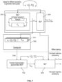
- Figure 1 shows a highly schematic block diagram of a runtime stack 100 for an autonomous vehicle (AV).
- the run time stack 100 is shown to comprise a perception stack 102, a prediction stack 104, a planner 106 and a controller 108.
- the perception stack 102 receives sensor outputs from an on-board sensor system 110 of the AV.
- the on-board sensor system 110 can take different forms but generally comprises a variety of sensors such as image capture devices (cameras/optical sensors), LiDAR and/or RADAR unit(s), satellite-positioning sensor(s) (GPS etc.), motion sensor(s) (accelerometers, gyroscopes etc.) etc., which collectively provide rich sensor data from which it is possible to extract detailed information about the surrounding environment and the state of the AV and any external actors (vehicles, pedestrians, cyclists etc.) within that environment.
- image capture devices cameras/optical sensors
- LiDAR and/or RADAR unit(s) satellite-positioning sensor(s) (GPS etc.)
- GPS etc. satellite-positioning sensor(s)
- motion sensor(s) accelerelerometers, gyroscopes etc.
- the sensor outputs typically comprise sensor data of multiple sensor modalities such as stereo images from one or more stereo optical sensors, LiDAR, RADAR etc.
- Stereo imaging may be used to collect dense depth data, with LiDAR/RADAR etc. proving potentially more accurate but less dense depth data. More generally, depth data collection from multiple sensor modalities may be combined in a way that respects their respective levels (e.g. using Bayesian or non-Bayesian processing or some other statistical process etc.). Multiple stereo pairs of optical sensors may be located around the vehicle e.g. to provide full 360° depth perception. This provides a much richer source of information than is used in conventional cruise control systems.
- the perception stack 102 comprises multiple perception components which co-operate to interpret the sensor outputs and thereby provide perception outputs to the prediction stack 104.
- the perception outputs from the perception stack 102 are used by the prediction stack 104 to predict future behaviour of the external actors.
- Predictions computed by the prediction stack 104 are provided to the planner 106, which uses the predictions to make autonomous driving decisions to be executed by the AV in a way that takes into account the predicted behaviour of the external actors.
- the planner 106 implements the techniques described below to plan trajectories for the AV and determine control actions for realizing such trajectories.
- a core function of the planner 106 is to determine a series of control actions for controlling the AV to implement a desired goal in a given scenario.
- a scenario is determined using the perception stack 102 but can also incorporate predictions about other actors generated by the prediction stack 104.
- a scenario is represented as a set of scenario description parameters used by the planner 106.
- a typical scenario would define a drivable area and would also capture predicted movements of any obstacles within the drivable area (such as other vehicles) along with a goal.
- a goal would be defined within the scenario, and a trajectory would then need to be planned for that goal within that scenario.
- obstacles are represented probabilistically in a way that reflects the level of uncertainty in their perception within the perception stack 102.
- the goal could for example be to enter a roundabout and leave it at a desired exit; to overtake a vehicle in front; or to stay in a current lane at a target speed (lane following).
- the goal may, for example, be determined by an autonomous route planner (not shown).
- the controller 108 executes the decisions taken by the planner 106 by providing suitable control signals to on-board actuators 112 such as motors of the AV.
- the controller 108 controls the actuators in order to control the autonomous vehicle to follow a trajectory computed by the planner 106.
- the planner 106 plans over acceleration (magnitude) and steering angle control actions simultaneously, which are mapped to a corresponding trajectory by modelling the response of the vehicle to those control actions. This allows constraints to be imposed both on the control actions (such as limiting acceleration and steering angle) and the trajectory (such as collision-avoidance constraints), and ensures that the final trajectories produced are dynamically realisable.
- the planner 106 will determine an optimal trajectory and a corresponding sequence of control actions that would result in the optimal trajectory according to whatever vehicle dynamics model is being applied.
- the control actions determined by the planner 106 will not necessarily be in a form that can be applied directly by the controller 108 (they may or may not be).
- control data is used herein to mean any trajectory information derived from one of both of the planned trajectory and the corresponding series of control actions that can be used by the controller 108 to realize the planner's chosen trajectory.
- the controller 108 may take the trajectory computed by the planner 106 and determine its own control strategy for realizing that trajectory, rather than operating on the planner's determined control actions directly (in that event, the controller's control strategy will generally mirror the control actions determined by the planner, but need not do so exactly).
- the planner 106 will continue to update the planned trajectory as a scenario develops. Hence, a trajectory determined at any time may never be realized in full, because it will have been updated before then to account for changes in the scenario that were not predicted perfectly.
- the present disclosure addresses the planning problem of determining an optimal series of control actions (referred to herein as a "policy") for a given scenario and a given goal as a constrained optimization problem with two optimization stages.
- a polyicy an optimal series of control actions
- the first optimization stage solves a Mixed Integer Linear Programming (MILP) problem where obstacles lead to hard constraints for the MILP.
- MILP Mixed Integer Linear Programming
- the outcome of this seeds (initializes) a subsequent nonlinear optimisation of the trajectory for dynamics and comfort constraints, in the second optimization stage.
- the second optimization stage solves a Non-Linear Programming (NLP) problem, initializing using the results of the MILP optimization stage.
- NLP Non-Linear Programming
- the MILP stage uses a mixed-integer formulation of collision avoidance and drivable area constraints as described later.
- the NLP stage is described first, in order to set out the final planning problem that ultimately needs to be solved (Problem 2 below), and to provide some context for the subsequent description of how best to provide an effective initialization (seed) from the MILP stage.
- a vehicle whose motion is being planned is referred to as the ego vehicle.
- the ego state at time 0 is given by X 0
- a function of the planner 106 is to determine the ego states over the next N steps, X 1 : N ⁇ W X N .
- the set of the mean poses of all traffic participants over time is O 0 : N 1 : n , and similarly for the covariances ⁇ 0 : N 1 : n , and both are given as inputs to the planning problem.
- the global coordinate frame is transformed to a reference path-based representation under an invertible transform as described in Sec. II-B.
- This representation significantly simplifies the problem of path tracking.
- a goal of the ego vehicle is defined as following a differentiable and bounded two-dimensional reference path in the global coordinate frame, , parameterized by the distance from the start of the path X P ref ⁇ , Y P ref ⁇ .
- the reference path is a path which the ego vehicle is generally intending to follow, at a set target speed. However, deviation from the reference path and target speed, whilst discouraged, are permitted provided that no hard constraints (such as collision avoidance constraints) are breached.
- the reference path can be determined using knowledge of the road layout, which may use predetermined map data (such as an HD map of the driving area), information from the perception stack 104, or a combination of both. For complex layouts in particular (such as complex junctions or roundabouts), the reference path could be learned by monitoring the behaviour of other drivers in the area over time.
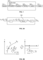
- Figure 2A illustrates the process of going from an input ( X 0 , O 0 : N 1 : n , ⁇ 0 : N 1 : n ) to the desired output X 1 : N .
- the output of the planner 106 is an intended trajectory x 0: N in the reference path-based representation, which in turn is transformed back to the global coordinate frame by applying the inverse transformation to obtain X 0: N in the global coordinate frame. Further details of the transformation are described below.
- the invertible transform operates over three types of input: (1) poses, (2) velocities and (3) covariance matrices. Each of the individual operations is described next.
- the ego vehicle is modelled as a rigid body occupying an area S e ⁇ R 2 relative to its center, and the area occupied by the ego vehicle at state x k is given by
- the area each traffic participant occupies is defined as with probability larger than p ⁇ .
- a cost function J x 0 : N u 0 : N ⁇ 1 o 0 : N 1 : n ⁇ 0 : N 1 : n defined over the positions and controls of the ego vehicle and states and uncertainties of other traffic participants, a "policy synthesis" problem can be formulated.
- a "policy” in the present context refers to a time-series of control actions, which is mapped to a corresponding vehicle trajectory using a vehicle dynamics model.
- the hard constraints comprise (1) vehicle model constraints, including kinematic ones on the transitions of the model and on the controls it allows (Sec. III-1); and (2) collision avoidance constraints with the purpose of avoiding collisions with the boundaries of the road (which can include, e.g. construction areas or parked vehicles) as well as other traffic participants (Sec. III-2).
- Soft constraints make up the terms of the cost function (i.e. are embodied in the cost function itself) and are presented in Sec. III-3, whereas hard constraints constrain the optimization of the cost function. Sec. III-4 describes the full problem.
- x k + 1 ⁇ ⁇ t x k u k ⁇ k ⁇ ⁇ max a min ⁇ a k ⁇ a max a k + 1 ⁇ a k ⁇ a ⁇ max ⁇ k + 1 ⁇ ⁇ k ⁇ ⁇ max ⁇ min ⁇ ⁇ k ⁇ ⁇ max b l x k z ⁇ y k z ⁇ b r x k z , z ⁇ Z g i , z x k > 1 , i ⁇ 1 , ... n , z ⁇ Z
- the tuple ( x 0 , O 0 : n 1 : N , ⁇ 0 : n 1 : N ) is an example of a set of scenario description parameters, describing a dynamic scenario and a starting state of the ego vehicle within it.
- the dynamics of the scenario is captured in terms of the motion components of x 0 , O 0 : n 1 : N and ⁇ 0 : n 1 : N , i.e. the speed and heading dimensions within the NLP formulation.
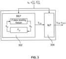
- Figure 3 shows a two-tier optimization architecture: a first stage 302 corresponds to solving a receding horizon formulation of the linearized version of the problem; in a second stage 304, the problem is solved in a non-linear non-convex constrained optimization fashion using the solution of the first stage as an initialization.
- the two stage optimisation of Figure 3 may be referred to as 2s-OPT.
- a motivation behind the architecture is to avoid the local optima convergence in the non-linear, non-convex constrained optimization by providing an initial solution that is closer to the global optimum, which also should lead to faster and more reliable convergence.
- the first stage 302 solves a linearized version of Problem 2 in a finite, receding horizon manner using a Mixed Integer Linear Programming (MILP) formulation (details presented in Sec. IV-A).
- MILP Mixed Integer Linear Programming
- the second stage 304 uses the output of the MILP optimizer as an initial solution and solves the full Problem 2, as set out above. Given the similar representations of the linearized and non-linear problems, it is expected that this initialization improves convergence, speed and the quality of the final solution.
- Problem 2 is re-formulated as a Mixed Integer Linear Programming optimization problem, with mixed integer linear constraints and a multi-objective cost function.
- This representation is still based on the reference path , and is the same as the representation used in the second stage 304 in terms of the spatial dimensions.
- the second stage 304 uses an angular representation of motion (i.e. velocity and acceleration are represented in terms of magnitude and angle components)
- the first stage uses a linear representation of velocity and acceleration.
- Similar constraints are imposed as in the non-linear model of the second stage 304, in particular input bounds constraints, a x min ⁇ a x k ⁇ a x max and a y min ⁇ a y k ⁇ a y max ; jerk related constraints, a k + 1 x ⁇ a k x ⁇ ⁇ a max x ⁇ t and a k + 1 y ⁇ a k y ⁇ ⁇ a max y ⁇ t ; and velocity constraints v x min ⁇ v x k ⁇ v x max and v y min ⁇ v y k ⁇ v y max , with v x min ⁇ 0 to guarantee forwards motion.
- piecewise-linear functions b l M x and b r M x are defined for the left and right road boundaries respectively, such that ⁇ x : b l M x ⁇ b r M x .
- the constraint is formulated as: d + b l M x k ⁇ y k ⁇ b r M x k ⁇ d
- d is a function of the size of the ego vehicle with respect to its point estimate.
- d w 2 + l 2 / 2 , i.e. reduce the driveable surface to where ⁇ is the Minkowski-sum operator.
- the ellipses L a k i b k i defined in (9) are inscribed with axis-aligned rectangles, which are then augmented to consider the point estimate of the ego vehicle's pose.
- x k , min i , x k , max i , y k , min i , y k , max i can be computed in closed form from L a k i b k i , d x and d y .
- the collision avoidance constraint is the logical implication: x k , min i ⁇ x ⁇ x k , max i ⁇ y ⁇ y k , min i ⁇ y ⁇ y k , max i which can be understood as "if the ego position is aligned with the vehicle along x, then it must be outside the vehicle's borders in y".
- the cost function of the MILP stage 302 should be similar to the cost function from the non-linear stage 304 to minimize the gap between the optimum obtained in both stages.
- the optimal trajectory computed in the first stage 302 should approximate the final optimal trajectory computed in the second stage 304, and therefore provide a useful initialization.
- MILP Problem Definition With constraints C and cost function the planning problem of the first stage 302 is formulated as a MILP problem with a receding horizon of K steps.
- a full trajectory x 0: N of length N +1 is obtained at the first stage 302, to initialize the second stage 304.
- the receding horizon approximation iteratively breaks the problem down into a set of simpler optimization problems, each defined over K ⁇ N steps.
- a "cost component" of the full cost function is defined as the sum of the individual costs over only K steps, as set out below.
- x ⁇ k + 1 F ⁇ t x ⁇ k u ⁇ k a min x ⁇ a k x ⁇ a max x a min y ⁇ a k y ⁇ a max y a k + 1 x ⁇ a k x ⁇ ⁇ a max x ⁇ t a k + 1 y ⁇ a k y ⁇ ⁇ a max y ⁇ t ⁇ min x ⁇ ⁇ k x ⁇ ⁇ max x ⁇ min y ⁇ ⁇ k y ⁇ ⁇ max y ⁇ x ⁇ ⁇ ⁇ y d + b l M x k ⁇ y k y k ⁇ b r M x k ⁇ d y k , max i ⁇ M ⁇ k i
- the known initial vehicle state x 0 is used as a starting point, with subsequent states determined by applying the vehicle dynamics model F ⁇ t in an iterative fashion.
- the state x m -1 determined in the previous planning step m - 1 provides a starting point for that iteration, with subsequent states computed from that starting point in the same way.
- the state vectors of both the ego vehicles and the other actors, and control vectors are not restricted to integer values, or otherwise discretised to any fixed grid. Not discretizing over a grid is one of the advantages of the method, as it allows for smoother trajectories.
- the integer variables in the MILP stage are used to enforce the constraints related to collision avoidance and driveable surface only.
- the trajectory x 0: N computed in the MILP optimization stage 302 is an example is a "seed trajectory", as that term is used herein, whereas the trajectory x 0: N computed in the NLP optimization stage 304 (derived, in part, from the seed trajectory x 0: N ), is an example of a "final” trajectory.
- the trajectory is "final” within the specific context of the two-stage optimization.
- the term “final” does not necessarily imply finality within the context of the runtime 100 stack as a whole.
- the final trajectory x 0: N may or may not be subject to further processing, modification etc. in other parts of the runtime stack 100 before it is used as a basis for generating control signals within the controller 108.
- the linear cost function of Equation (22) and the linear dynamics model of Equations (15) and (16) are examples of a "preliminary" cost function and model respectively
- the non-linear cost function of Equation (11) and the non-linear dynamics model of Equation (5) are examples a “final” or, equivalently, “full” cost function and model respectively, where the terms “final” and “full” are, again, only used in the specific context of the two-stage optimization, and does not imply absolute finality.
- control actions u 0: N -1 of the MILP stage 302 are alternatively or additionally used to seed the NLP stage 304 (and they may be referred to as seed control actions in that event); similarly, as noted above, data of one or both of the final trajectory x 0: N and the final series of control actions u 0: N -1 may be provided to the controller 108 for the purpose of generating "actual" control signals for controlling the autonomous vehicle.
- the scenario description parameters ( x 0 , O 0 : n 1 : N , ⁇ 0 : n 1 : N ) have a non-linear form (because they are formulated in terms of heading ⁇ k )
- the scenario description parameters ( x 0 , O 0 : n 1 : N , ⁇ 0 : n 1 : N ) have a linear form (because motion is formulated in terms of components v k x , v k y instead of speed and heading v k , ⁇ k ) , with x 0 denoting the linearized form of the ego vehicle state specifically.
- x 0: N and x 0: N are used as shorthand to represent complete trajectories, including the (known) current state x 0 .
- the additional states actually determined in the relevant optimization stage 302, 304 are x 1: N and x 1: N , as depicted in Figure 3 .
- An overtaking goal is defined by way of a suitably distant reference location (not shown) on the reference path , ahead of the forward vehicle 402.
- the effect of the progress constraints is to encourage the ego vehicle 400 to reach that reference location as soon as it can, subject to the other constraints, whilst the effect of the collision avoidance constraints is to prevent the ego vehicle 402 from pulling out until the oncoming vehicle stops being a collision risk.
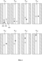
- Figure 5 illustrates some of the principles underlying the MILP formulation of the first stage 302.
- the ego vehicle 400 remains axially aligned (i.e. aligned with the reference path ) at all times.
- This reflects the simpler, linear dynamics model that is used in the MILP stage - as can be seen from Equations (15) and (16) above, the simpler dynamics model does not consider rotation of the ego vehicle 200 (recall that the MILP stage uses a linear representation of velocity and acceleration).
- the output of the first stage 302 is a more "restricted" form of trajectory defined in terms of linear position and velocity but not orientation/heading of the ego vehicle 200.
- the linearized trajectory may not be fully dynamically realisable, but nevertheless serves as a useful initialization to the second stage 304.
- the form of the trajectory planned in the second stage 304 is not restricted in the same way the first stage 302. This is because the full problem takes into account steering angle and heading of the ego vehicle 200. That is, the solution to Problem 2 is free to consider motion of the ego vehicle 400 that does not meet the discretisation restrictions applied in the first stage 302.
- a solution to Problem 3 can be obtained using Branch and Bound, a divide and conquer algorithm first introduced and applied to mixed integer linear programming by Land and Doig in [C-10]. This solution is proven to be the globally optimal one [C-7], [C-11].
- modern solvers e.g. Gurobi or CPLEX
- the receding horizon formulation of the problem introduced for the sake of computational tractability, generates suboptimality by definition [C-12], [C-13]. Due to these factors, no strong theoretical guarantee can be given regarding the solution of the MILP stage.
- a solution that is close to the global optimum at each receding horizon step acts as a proxy towards a final solution to be obtained in the second stage 304 that is close to the global optimum and, in turn, initializing the NLP stage using this solution is expected to improve the quality of the solution at that second stage 304.
- the speed increase provided by the two-stage approach will admit direct application on an autonomous vehicle in real-time.
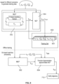
- Figure 6 shows how the two-stage optimization can be run repeatedly, in an offline context (e.g. in an off-board training computer system), for different scenarios, for the purpose of generating an NLP training set 600.
- each input in the NLP training set 600 corresponds to an initialization output generated by the first stage optimizer 302 on a given scenario, and a ground truth label for that inputs is given by the output of the second stage optimization 304 on that training scenario.
- the NLP optimization stage 304 is treated as a function that takes the initialization output of the first stage 302, and transforms it to a desired control output (corresponding the optimal trajectory solving Problem 2).
- a function approximator 304 can be trained to approximate this function of the NLP optimization stage 304.
- the trained function approximator 604 (which may be referred to as the NLP approximator 602) can, in turn, be implemented on-board the vehicle 400, rather than attempting to perform the full non-linear optimization of the second stage 304 on-board the vehicle in real-time.
- Each training example 601 of the NLP training set is made up of an input, which in turn comprises a particular set of scenario description parameters ( x 0 , O 0 : n 1 : N , ⁇ 0 : n 1 : N ) together with a corresponding seed trajectory x 0: N (i.e. as computed in the MILP stage 302 for the corresponding scenario description parameters), and a corresponding ground truth, which in this case is a corresponding final trajectory x 0: N as computed in the NLP stage 304 for the corresponding input.
- scenario description parameters x 0 , O 0 : n 1 : N , ⁇ 0 : n 1 : N
- a corresponding seed trajectory x 0: N i.e. as computed in the MILP stage 302 for the corresponding scenario description parameters
- a corresponding ground truth which in this case is a corresponding final trajectory x 0: N as computed in the NLP stage 304 for the corresponding input
- the NLP approximator 900 computes a corresponding final trajectory x ⁇ 0: N which will approximate a full NLP solution x 0: N that would be obtained from the full NLP optimization ( x 0: N may be referred to as the exact final trajectory in this context).
- a trajectory verification component 702 is provided, whose function is to verify the approximate final trajectory x ⁇ 0: N against the hard NLP constraints (i.e. the constraints as set out above in relation to Problem 2), or some practical variant of the hard NLP constraints (e.g.
- the NLP approximator 712 could be trained "conservatively" on somewhat more stringent hard constraints than the constraints the approximate final trajectory x ⁇ 0: N is actually required to satisfy, in order to reduce instances in which the approximate final trajectory x ⁇ 0: N fails the actual hard constraints imposed by the trajectory verification component 712). That is to say, the trajectory verification component 712 verifies the approximate final trajectory x ⁇ 0: N against a set of trajectory verification constraints, which may or may not be identical to the NLP constraints of Problem 2.
- the approximate final trajectory x ⁇ 0: N satisfies the trajectory verification constraints, it can be passed to the controller 108 to implement.
- the approximate final trajectory fails to satisfy at least one of the trajectory verification constraints, then it can modified, either at the planning level (by the planner 106) or control level (by the controller 108) so that it does. Assuming the NLP approximator 702 has been adequately trained such modifications, if required, should generally be relatively small.
- the different scenarios could, for example, be simulated scenarios, generated in a simulator.
- FIG. 7 shows how a similar approach may be adopted to approximate the MILP stage 302 online.
- a MILP training set 700 is created through repeated applications of the MILP optimizer on different scenarios, and each training example 701 of the MILP training set 700 is made up of an input in the form of particular set of scenario description parameters ( x 0 , O 0 : n 1 : N , ⁇ 0 : n 1 : N ) (mirroring the input to the MILP stage 302) and a corresponding ground truth, which is now the corresponding seed trajectory x 0: N (i.e. as obtained for the corresponding input parameters in the MILP stage 302).
- the seed trajectory x 0: N forms part of the input of each training example 601 of the NLP training set 600 of Figure 6 (with the full trajectory x 0 providing the ground truth), in the MILP training set 700 of Figure 7 , the seed trajectory x 0: N now provides the ground truth.
- a function approximator 702 is trained on the MILP training set 700 to approximate the MILP stage 602.
- Such a trained MILP approximator 702 can then be used in online processing to compute an approximate seed trajectory x ⁇ ⁇ 0 : N given a set of online scenario description parameters ( x 0 , O 0 : n 1 : N , ⁇ 0 : n 1 : N ), and the approximate seed trajectory x ⁇ ⁇ 0 : N can, in turn, be used to initialize an online instantiation of the NLP stage 304.
- the full NLP stage 304 is implemented, and the trajectory verification component 712 is therefore not required.
- x ⁇ 0: N and x ⁇ ⁇ 0 : N are used as shorthand to represent complete trajectories, including the current state x 0 .
- the states actually determined by the relevant function approximator are x ⁇ 1: N and x ⁇ ⁇ 1 : N .
- Certain figures show x ⁇ 0: N and x ⁇ ⁇ 0 : N as an output of a function approximator. It will be appreciated that this is a shorthand decision of the computed states x ⁇ 1: N / x ⁇ ⁇ 1 : N (as applicable), together with the known initial state x 0 provided as an input to the system. This also applies to Figures 8 and 9 (see below).
- Figure 8 shows an example of an implementation in which the MILP stage 302 and the NLP stage 304 are both approximated.
- the MILP approximator 702 of Figure 7 is used to seed the NLP approximator 604 of Figure 6 , i.e. an approximate seed trajectory x ⁇ ⁇ 0 : N forms an input to the NLP function approximator 604, which in turn is used in deriving an approximate full trajectory x ⁇ 0: N .
- the trajectory verification component 712 is used, as in Figure 6 , to verify the approximate full trajectory x ⁇ 0: N .
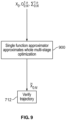
- Figure 9 shows another example implementation, in which a single function approximator 900 is trained to approximate both optimization stages 302, 304.
- the function approximator 900 takes, as input, a set of scenario description parameters, and directly computes an approximate full trajectory x ⁇ 0: N .
- the single approximator 900 would be trained on training examples whose inputs are scenario description parameters and whose ground truths are provided by the corresponding full NLP trajectories.
- a trajectory verification component 732 is similarly used in this case to verify the output of the single function approximator 900.
- the term "approximate" is used herein in two somewhat distinct senses.
- the MILP / NLP function approximator 302 / 304 is said to approximate the seed trajectory x 0: N / final trajectory x 0: N as applicable (i.e.
- the output of the trained MILP approximator 702, x ⁇ ⁇ 0 : N is said to be an approximation of the exact seed trajectory x 0: N that would be derivable via the full MILP optimization; likewise, the output of the trained NLP approximator 704, ⁇ x 0: N , is said to be an approximation of the exact final trajectory x 0: N that would be obtained via the full NLP optimization).
- the seed trajectory x ⁇ 0 : N / x ⁇ ⁇ 0 : N (whether exact or approximate in the sense of the preceding paragraph) is also said to approximate the full trajectory x 0: N / x ⁇ 0: N (whether exact or approximate in the sense of the preceding paragraph).
- the exact or approximate seed trajectory x ⁇ 0 : N / x ⁇ ⁇ 0 : N may be a relatively coarse approximation of the exact or approximate final trajectory x 0: N / x ⁇ 0: N .
- a relatively coarse approximation in this context is perfectly acceptable, because even a coarse seed trajectory (i.e.
- Equation (22) approximates the non-linear cost function of Equation (11) and the linear dynamics model of Equations (15) and (16) approximates the non-linear dynamics model of Equation (5).
- each approximator 602, 704 could alternatively or additionally be trained to determine an approximate series of seed control actions u ⁇ ⁇ 0 : N ⁇ 1 (approximating those of the MILP stage 302) and/or an approximate series of final control actions ⁇ 0: N -1 (approximating those of the NLP stage 304 - and which could in turn form (part of) or be used to derive the input to controller 108).
- each approximator 602, 704 could alternatively or additionally be trained to determine an approximate series of seed control actions u ⁇ ⁇ 0 : N ⁇ 1 (approximating those of the MILP stage 302) and/or an approximate series of final control actions ⁇ 0: N -1 (approximating those of the NLP stage 304 - and which could in turn form (part of) or be used to derive the input to controller 108).
- the same applies to the single approximator of Figure 9 which could alternatively or additionally compute ⁇ 0: N -1 directly from the scenario description parameters
- the above techniques be implemented in an "onboard” or “offboard” context.
- One example of an offboard context would be the above training performed in an offboard computer system.
- the above techniques can also be implemented as part of a simulated runtime stack in order to test the performance of the runtime stack in a simulator. Simulation is an increasingly crucial component of safety and other performance testing for autonomous vehicles in particular.
- the function approximator(s) can be tested in the simulator, in order to assess their safety and performance before they are deployed on an actual vehicle.
- V. PILOT Efficient Planning by Imitation Learning and Optimisation for Safe Autonomous Driving
- PILOT Planning by Imitation Learning and Optimisation
- PILOT planner Planning by Imitation Learning and Optimisation
- a PILOT planner could be implemented in the architecture of Figure 7 .
- a PILOT planner could be implemented the architecture of Figure 8 or Figure 9 , in which the verification component 712 also takes the form of a runtime optimizer.
- the architecture of Figure 9 is used, i.e. a single function approximator 900 is trained to imitate both the MILP and NLP stages 302, 304, and the verification component 712 is implemented using the same logic as the NLP stage 304, i.e. the functionality described in section III is implemented in two contexts - firstly, as part of the process to generate training data for the single function approximator 604, and secondly to refine an initial trajectory provided by the trained function approximator 900 at runtime.
- NLP logic would be applied to generate the training data for the second function approximator 604, and also at runtime to implement the verification component 712.
- PILOT architecture provides high-quality solutions by avoiding convergence to local optima, it can do so in real-time, even on a resource-constrained platform such as an autonomous vehicle or other mobile robot computer system.
- Guaranteeing safety of decision making is a fundamental challenge in the path towards the long-anticipated adoption of autonomous vehicle technology. Attempts to address this challenge show the diversity of possible definitions of what safety means: whether it is maintaining the autonomous system inside a safe subset of possible future states [D-1], [D-2], preventing the system from breaking domain-specific constraints [D-3], [D-4], or exhibiting behaviours that match the safe behaviour of an expert [D-5], amongst others.
- model-based approaches to safety are engineering-heavy and require deep knowledge of the application domain, while, on the other hand, the hands-off aspect of the data-driven approach is lucrative, hence the growing interest in the research community in exploiting techniques like imitation learning for autonomous driving [D-6], [D-7], [D-8], [D-9].
- inference using a data-driven model is usually very efficient compared to, e.g., more elaborate search- or optimisation-based approaches.
- model-based planning approaches give a better handle on understanding system expectations through model specification and produce more interpretable plans [D-10], [D-11], [D-12], but usually at the cost of robustness [D-13] or runtime efficiency [D-4].
- the imitation learning approach taught herein is generally applicable, and can be used to approximate any desired reference planner.
- the following examples use the two-stage optimisation approach of Figure 3 as the base planner, which produces high-quality plans by solving two consecutive optimisation problems but struggles in runtime efficiency. However, it will be appreciated that the description applies equally to any reference planner.
- a benefit of the multi-stage optimization-based architecture of Figure 3 is that better solutions can be achieved at the expense of increased computing resources (i.e. there is a direct relationship between the resources allocated to the planner and the quality of the final trajectories it produces).
- the non-real-time expert planner provide high quality expert trajectories, which can then be used to train a real-time planner (e.g. neural network-based) via imitation learning.
- the following examples use an in-the-loop DAgger [D-17] approach to imitation learning to train a deep neural network to imitate the output of the expert planner.
- Online augmentation using DAgger enriches the learner's dataset with relevant problem settings that might be lacking in the expert planner's dataset. This benefits from the fact that (unlike a human expert) the expert planner of Figure 3 is always available to update the training dataset and label new instances experienced by the learner with expert output, leading to much reduced training cost compared to using human expert data.
- this targeted augmentation is in contrast to other dataset augmentation techniques that rely on random perturbations to the expert problems, e.g. [D-19],[D-21].
- a constrained optimisation step is applied, that uses a similar objective function to the expert's, to smooth and improve upon the resulting trajectory from a safety perspective.
- This uses the architecture of Figure 9 , with the single function approximator 900 (a deep neural network in the following examples) trained to imitate the full expert panner of Figure 3 (i.e. both the first and second stages 302, 304), and the verification component 712 implemented using the same constrained optimizer as the second stage 304 or a similar constrained optimizer (that is seeded with a high quality solution from the trained function approximator 900 and can operate in runtime).
- the trajectory verification component 712 receives a trajectory from the neural network 900, which is used to seed a further non-linear optimization performed by the trajectory verification component 712.
- the further non-linear optimization may result in a modified trajectory that is guaranteed to satisfy whatever constraints are imposed by the trajectory verification component 712.
- the trajectory verification component 712 may be referred to as a "runtime” or "post-hoc" optimizer (to distinguish from the optimization stages 302, 304 of the expert planner).
- Another benefit of imitating an optimisation-based system rather than human data is a much reduced training cost, especially with regard to updating the training dataset and labelling new instances experienced by the learner with expert output.
- an optimization-based system can also be used to generate training data for simulated scenarios.
- the performance of the present imitation learning and optimisation architecture has been evaluated on sets of simulated experiments generated using a light-weight simulator and using CARLA [D-22], and compared in terms of trajectory cost and runtime to the optimisation planner it is based on, as well as to other alternative architectures that employ the same optimisation component as PILOT.
- one aspect herein is an efficient and safe planning framework for autonomous driving, comprising a deep neural network followed by a constrained optimisation stage.
- Another aspect is process of imitating a model-based optimiser to improve runtime efficiency.
- the PILOT solution improves the efficiency of expensive-to-run optimisation-based planners.
- v is defined to be an efficient optimiser that solves Eq. D-1 (e.g.
- ⁇ can be an expert expensive-to-run optimisation procedure that attempts to improve upon the local optimum of Eq. D-1 found by v .
- Examples of ⁇ can include performing a recursive decomposition of the problem and taking the minimum cost [D-27] or applying other warm-starting procedures [D-4],[D-28].
- PILOT The goal of PILOT is to achieve the lower cost on provided by ⁇ , while approximating the efficient runtime of ⁇ . To do so, PILOT employs an imitation learning paradigm to train a deep neural network, (900, Figure 9 ), that imitates the output of ⁇ , which it then uses to initialise v in order to output a feasible and smooth trajectory.
- the base planner is implemented using the 2s-OBT framework of Figure 3 , in which a planning architecture comprising a sequence of two optimisation stages is introduced for autonomous driving.
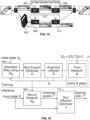
- Fig 15 shows the architecture of the 2s-OPT planner, as in Figure 3 .
- the input to the system are: 1) a birds-eye view of the planning situation, that includes the ego vehicle, other road users and the relevant features of the static layout; 2) a route plan as a reference path, provided by an external route planner; and 3) predicted traces for all road users, provided by a prediction module.
- the first optimisation stage 302 solves a linearised version of the planning problem using a Mixed Integer Linear Programming (MILP) solver.
- MILP Mixed Integer Linear Programming
- the output of the MILP solver is fed as a warm-start initialisation to a constrained, non-linear optimiser 304.
- This second optimisation stage ensures that the output trajectory is smooth and feasible, while maintaining the safety guarantees.
- PILOT is used with the two stage optimisation (2s-OPT) approach of Figure 3 as the base planner.
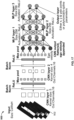
- a convolutional neural network is 900 to take as input a graphical representation 902 of the reference path-projected planning situation (including predictions of other road users) in addition to other scalar parameters of the problem (e.g., speed of the ego vehicle), and output a smooth trajectory that imitates the output of the optimiser when presented with the same problem.
- 2s-OPT is run on a dataset of problems to initiate the training, and uses to label the new planning problems generated by the learner in simulations.
- the post-hoc optimizer 712 implements a nonlinear constrained optimisation stage, similar to the second stage 304 in 2s-OPT to maintain safety and smoothness guarantees.
- C greyscale top-down images of the scene of size W ⁇ H are produced by uniformly sampling in time the positions of road users along their predicted trajectories at times t ⁇ 0 , h C ⁇ 1 , ... h for the planning horizon h.
- These images create an input tensor of size C ⁇ W ⁇ H, allowing convolutional layers to be used to extract semantic features of the scene and its temporal evolution.
- the static layout information is present on all channels.
- Additional information of the planning problem that is not visualised in the top-down images (such as the initial speed of the ego vehicle) are appended as scalar inputs, along with the flattened convolutional neural network (CNN) output, to the first dense layer of the network.
- CNN convolutional neural network
- Figure 17 shows further details of an example convolutional architecture for the neural network 900.
- the output of the network is a trajectory in the reference path coordinate frame.
- an alternative is to train the network to produce parameters for smooth function families, e.g. polynomials and B-splines, over time, namely f x ( t ) and f y ( t ).
- the post-hoc NLP optimisation stage (detailed below) expects as input a time-stamped sequence of states, each comprising: ( x,y ) position, speed, orientation and control inputs (steering and acceleration), all in the reference path coordinate frame. Velocities and orientations are calculated from the sequence of points produced by the network (or sampled from the smooth function output). Control input is derived from an inverse dynamics model.
- a scenario state in this context is a snapshot of a scene at a given time instant with an ego (simulated agent or real vehicle) to plan for and all other agents' trajectories having been predicted.
- Figure 16 shows a schematic block diagram of a PILOT training scheme.
- PILOT uses an expert-in-the-loop imitation learning paradigm to train a deep neural network, (900), that imitates the output of the expensive-to-run optimisation-based planner ⁇ (top). At inference time, it uses the output of to initialise an efficient optimiser v (712) to compute a feasible and low-cost trajectory (bottom).
- the scheme alternates between training steps and augmentation steps.
- the first training set is performed on a large dataset of examples obtained using the reference planner ⁇ .
- the parameters ⁇ are tuned via training on an augmented training set , as augmented in the previous augmentation step.
- the (partially trained) network 900 is applied to simulated scenarios in a simulator 904, by using the partially trained network 900 to plan trajectories for a simulated ego agent (typically in response to other agent(s) in the scenario).
- the expert planner ⁇ is then applied in "shadow mode", i.e.
- the reference planner ⁇ is used to generate expert trajectories at those time instants, which in turn are used to augment the training set for the next training step.
- the evolution of each simulated scenario is determined, at least in part, by the actions of the partially trained network 900 (for example, at some time into the scenario, x 0 would generally depend on earlier actions by the partially trained network 900, as may the other parameters O 0 : n 1 : N , ⁇ 0 : n 1 : N e.g.
- the reference planner ⁇ then provides expert trajectories for those scenarios (but, unlike the network 900, does not control the ego agent or influence the simulated scenarios, because the aim is to expose the reference planner ⁇ to scenarios in which errors by the partially trained network 900 might have accumulated over time).
- z k [ x k , y k , ⁇ k , v k ] T describes the state of the ego at time k with ( x k , y k ) being the reference-path projected position, ⁇ k is the vehicle's yaw angle, and v k is its speed.
- Constraints are enforced that maintain acceleration and steering values within the permitted ranges, limit maximum jerk and angular jerk, and maintain speed within the allowed speed limit for the road. Also, constraints are added that ensure that the corners of the ego vehicle's footprint are at all times bounded within the road surface, and that prevent collision with other road users.
- ⁇ i ⁇ R are scalar weights
- ⁇ i ( z k , u k ) are soft constraints that measure deviation from the desired speed, the reference path and the end target location, and that control the norms of acceleration and steering control inputs.
- Parameters of the optimisation are fine-tuned using grid-search in the parameter space. See Annex B for a more detailed formulation of the optimisation problem.
- the output of the imitation learning neural network is used as an initialisation to this optimisation problem.
- the initialisation trajectory is processed to cap abnormal values of calculated speed, acceleration and steering that might break some of the hard constraints. The process is detailed in Annex C.
- a function approximator takes the form of one or more trainable models than can be trained to imitate an expert.
- Those models can take any form, including but not limited to neural network(s).
- the expert may be a computer-implemented planner (not necessarily required to operate in real-time), as in the above examples.
- the one or more models are chosen so that they can be applied with fewer computing resources or memory resources than the expert planner (preferably in real-time).
- this issue is addressed by implementing the NLP logic at runtime, to refine the initial trajectory produced by the function approximator, and in this context it is not necessary for the trained function approximator to perfectly imitate the expert.
- the function approximator can be trained to implement other types of planner.
- the expert planner has the ability to produce high-quality trajectories, but requires significant computational and/or memory resources to do so. It also feasible to use a human expert(s) to provide at least some of the training data for the function approximator.
- a computer system comprises one or more computers that may be programmable or non-programmable.
- a computer comprises one or more processors which carry out the functionality of the aforementioned functional components.
- a processor can take the form of a general-purpose processor such as a CPU (Central Processing unit) or accelerator (e.g. GPU) etc. or more specialized form of hardware processor such as an FPGA (Field Programmable Gate Array) or ASIC (Application-Specific Integrated Circuit).
- CPU Central Processing unit
- accelerator e.g. GPU
- FPGA Field Programmable Gate Array
- ASIC Application-Specific Integrated Circuit
- a processor may be programmable (e.g. an instruction-based general-purpose processor, FPGA etc.) or non-programmable (e.g. an ASIC).
- a computer system may be implemented “onboard” a mobile robot (such as an AV) or “offboard” for example in a simulator context.
- an offboard implementation of the full multi-stage optimization could be implemented for the purpose of training on-board components, but also for other purposes, such as safety testing or other performance testing, verification etc.
- Performance testing could involve implementing any of the above trained function approximators 702, 604, 900 and (where applicable) the verification component 712 in an offboard computer system as part of the performance testing, applied to simulated scenarios.
- the multi-phase optimization may be implemented in full, or one or more (including all) optimization stages may be replaced with one or more function approximators.
- Annex E documents experimental results that demonstrate the efficacy of the PILOT architecture (as described in Section V.).
- Figure 10 shows, in the top half, an overtaking scenario somewhat analogous to that of Figures 4 and 5 .
- the top scenario of Figure 10 shows a scenario with overtaking of static vehicles 402 with an oncoming vehicle 404 in residential driving.
- FIG. 10 shows an alternative, junction scenario, which uses like reference numerals to denote the ego vehicle 400 and an external actor 402. This is an unprotected right turn in a junction.
- Figures 11 and 12 show two qualitatively distinct driving situations.
- the ego-vehicle overtakes parked vehicles on a two-lane road while taking into account an oncoming vehicle on the other lands that is also overtaking a static vehicle in its own lane (the reference path) for overtaking, and returning to it as soon as possible, while always maintaining a smooth acceleration profile.
- the second example in Figure 12 shows an unprotected right turn into a main road.
- Figure 12(d) shows the ego-vehicle closely reference path (right turn into the main road) while smoothly responding to unforeseen behaviors of the dynamic vehicles.
- Figure 13 shows examples of the four different simulation scenarios we consider for experiments 2) and 3): (SO) static overtaking of parked vehicles on both side of the road; (SO+OV) static overtaking with a dynamic vehicle in the oncoming lane; (DO) dynamic overtaking of a slow moving vehicle; and (DO+OV) dynamic overtaking with an oncoming vehicle on the other lane.
- SO static overtaking of parked vehicles on both side of the road
- SO+OV static overtaking with a dynamic vehicle in the oncoming lane
- DO dynamic overtaking of a slow moving vehicle
- DO+OV dynamic overtaking with an oncoming vehicle on the other lane.
- Table D-I presents the percentage of solved examples within the allocated time (25s) per initialization method and scenario. As it can be observed, our method either performs similarly or outperforms other methods in all the scenarios considered.
- Figure 14 we analyze the problems that were solved using our initialization when compared to the other initialization methods. We observe that, across scenarios ZEROS and C.DEC lead to the highest percentage of solved problems (after ours) and same solutions, but also the highest percentage of different solutions.
- Table II shows the average % difference in cost that the alternatives achieve compared to ours.
- Table II presents the average % difference in solving time.
- the network produces a sequence of spatial positions, and the rest of the required input of the optimiser are computed from that sequence. A number of checks of upper and lower limits are applied to tame abnormalities in the network output and to improve the input to the optimiser.
- the first experiment uses a training dataset of 70,000 procedurally-generated problems of two-lane, urban driving in a residential setting.
- the problems are generated from 33 manually-designed base scenarios that contain a mixture of static and moving vehicles.
- the ego vehicle's position, heading and speed are perturbed at different timesteps of the original scenarios to create new configurations.
- Each of these configurations is considered a planning problem and solved by 2s-OPT, creating a high-quality expert dataset.
- the training dataset is augmented with new problems generated interactively by the trained network when used in a driving simulator on new problems similar to the ones in the dataset.
- the new problems are solved by 2s-OPT as well to provide the expert trajectories.
- the second experiment uses the CARLA simulator [D-22] where we generate 20,000 planning instances by running a baseline planner in randomly-generated scenarios in Town02, and compute their 2s-OPT solutions, to train PILOT. Then we run DAgger training on Town02 using the CARLA simulator and CARLA's Autopilot to control all non-ego agents. Lastly, we benchmark PILOT on a dataset generated in Town01 using 2s-OPT. More details about the process are in Appendix D.
- Table D-II INITIALISATION ABLATION - NLP COMPARISON RELATIVE TO 2S-OPT IN AVERAGE SOLVING TIME AND FINAL NLP COST (IN PROBLEMS SOLVED BY 2s-OPT AND THE PARTICULAR INITIALISATION) AND CONVERGENCE RATE.
- PII,OT's neural network initialisation produces trajectories that are easier to optimise (as reflected in the reduction in NLP solving time) with a small increase in the final cost in average when compared to the MILP initialisation of 2s-OPT.
- One of the alternatives (ConstAccel) has a slight advantage in final NLP cost, but it takes more time when it converges and it fails to converge in 9% more examples to a solution.
Landscapes
- Engineering & Computer Science (AREA)
- Automation & Control Theory (AREA)
- Radar, Positioning & Navigation (AREA)
- Remote Sensing (AREA)
- Physics & Mathematics (AREA)
- General Physics & Mathematics (AREA)
- Aviation & Aerospace Engineering (AREA)
- Transportation (AREA)
- Mechanical Engineering (AREA)
- Electromagnetism (AREA)
- Human Computer Interaction (AREA)
- Business, Economics & Management (AREA)
- Artificial Intelligence (AREA)
- Evolutionary Computation (AREA)
- Game Theory and Decision Science (AREA)
- Medical Informatics (AREA)
- Health & Medical Sciences (AREA)
- Computer Vision & Pattern Recognition (AREA)
- Multimedia (AREA)
- Control Of Position, Course, Altitude, Or Attitude Of Moving Bodies (AREA)
- Manipulator (AREA)
Applications Claiming Priority (6)
| Application Number | Priority Date | Filing Date | Title |
|---|---|---|---|
| GBGB2001200.1A GB202001200D0 (en) | 2020-01-28 | 2020-01-28 | Planning in mobile robots |
| GBGB2001202.7A GB202001202D0 (en) | 2020-01-28 | 2020-01-28 | Planning in mobile robots |
| GBGB2001277.9A GB202001277D0 (en) | 2020-01-30 | 2020-01-30 | Planning in mobile robots |
| GBGB2017252.4A GB202017252D0 (en) | 2020-10-30 | 2020-10-30 | Planning in mobile robots |
| PCT/EP2021/052036 WO2021152047A1 (en) | 2020-01-28 | 2021-01-28 | Planning in mobile robots |
| EP21702929.7A EP4081876B1 (de) | 2020-01-28 | 2021-01-28 | Planung bei mobilen robotern |
Related Parent Applications (1)
| Application Number | Title | Priority Date | Filing Date |
|---|---|---|---|
| EP21702929.7A Division EP4081876B1 (de) | 2020-01-28 | 2021-01-28 | Planung bei mobilen robotern |
Publications (3)
| Publication Number | Publication Date |
|---|---|
| EP4361753A2 true EP4361753A2 (de) | 2024-05-01 |
| EP4361753A3 EP4361753A3 (de) | 2024-07-17 |
| EP4361753B1 EP4361753B1 (de) | 2025-10-22 |
Family
ID=74505218
Family Applications (2)
| Application Number | Title | Priority Date | Filing Date |
|---|---|---|---|
| EP21702929.7A Active EP4081876B1 (de) | 2020-01-28 | 2021-01-28 | Planung bei mobilen robotern |
| EP24163038.3A Active EP4361753B1 (de) | 2020-01-28 | 2021-01-28 | Planung bei mobilen robotern |
Family Applications Before (1)
| Application Number | Title | Priority Date | Filing Date |
|---|---|---|---|
| EP21702929.7A Active EP4081876B1 (de) | 2020-01-28 | 2021-01-28 | Planung bei mobilen robotern |
Country Status (3)
| Country | Link |
|---|---|
| US (1) | US12547175B2 (de) |
| EP (2) | EP4081876B1 (de) |
| WO (1) | WO2021152047A1 (de) |
Families Citing this family (50)
| Publication number | Priority date | Publication date | Assignee | Title |
|---|---|---|---|---|
| FR3074348B1 (fr) * | 2017-11-24 | 2020-09-11 | Dassault Aviat | Systeme de calcul de mission d'un aeronef comportant une platine de mission |
| EP4081876B1 (de) * | 2020-01-28 | 2024-04-10 | Five AI Limited | Planung bei mobilen robotern |
| EP4078320B1 (de) | 2020-01-28 | 2024-08-14 | Five AI Limited | Planung in mobilen robotern |
| US12187269B2 (en) * | 2020-09-30 | 2025-01-07 | Toyota Motor Engineering & Manufacturing North America, Inc. | Optical sense-compute solution for real-time navigation involving multiple vehicles |
| US12576864B2 (en) | 2020-10-30 | 2026-03-17 | Five AI Limited | Tools for performance testing and/or training autonomous vehicle planners |
| US20220219727A1 (en) * | 2021-01-12 | 2022-07-14 | Motional Ad Llc | Vehicle path planning |
| EP4298562A4 (de) * | 2021-02-25 | 2025-02-12 | Nanotronics Imaging, Inc. | Imitationslernen in einer fertigungsumgebung |
| CN112987762B (zh) * | 2021-05-10 | 2021-09-07 | 北京三快在线科技有限公司 | 一种轨迹规划方法、装置、存储介质及电子设备 |
| US11912311B2 (en) * | 2021-08-10 | 2024-02-27 | GM Global Technology Operations LLC | System and method of detecting and mitigating erratic on-road vehicles |
| CN113721607B (zh) * | 2021-08-16 | 2023-03-24 | 燕山大学 | 轮式机器人轨迹跟踪最优控制方法 |
| US12061474B2 (en) * | 2021-08-20 | 2024-08-13 | Mitsubishi Electric Research Laboratories, Inc. | Controller for optimizing motion trajectory to control motion of one or more devices |
| CN113759724B (zh) * | 2021-09-17 | 2023-08-15 | 中国人民解放军国防科技大学 | 基于数据驱动的机器人控制方法、装置和计算机设备 |
| EP4223616B1 (de) * | 2022-02-02 | 2025-12-31 | Aptiv Technologies AG | Verfahren und systeme zur seitlichen steuerung eines fahrzeugs |
| US20250145178A1 (en) | 2022-02-03 | 2025-05-08 | Five AI Limited | Trajectory generation for mobile agents |
| US12128923B2 (en) * | 2022-03-09 | 2024-10-29 | Gm Cruise Holdings Llc | Multi-objective bayesian optimization of machine learning model for autonomous vehicle operation |
| CN118922342A (zh) * | 2022-03-15 | 2024-11-08 | 华为技术有限公司 | 用于优化自动驾驶车辆运动规划器的系统和方法 |
| US12528505B2 (en) * | 2022-04-19 | 2026-01-20 | Gm Cruise Holdings Llc | Systems and methods for responding to detected emergency vehicles |
| CN114609918B (zh) * | 2022-05-12 | 2022-08-02 | 齐鲁工业大学 | 一种四足机器人运动控制方法、系统、存储介质及设备 |
| US12572154B2 (en) * | 2022-05-13 | 2026-03-10 | Mitsubishi Electric Research Laboratories, Inc. | System and method for controlling motion of one or more devices |
| WO2023219178A1 (en) * | 2022-05-13 | 2023-11-16 | Mitsubishi Electric Corporation | System and method for controlling motion of one or more devices along a calculated optimal trajectory |
| CN115016484B (zh) * | 2022-06-20 | 2025-03-11 | 清华大学深圳国际研究生院 | 一种基于采样和路径参数化的轨迹规划方法 |
| CN115099037B (zh) * | 2022-06-27 | 2024-11-29 | 清华大学 | 一种动力学模型支持的有偏好模仿学习方法及系统 |
| CN115042783A (zh) * | 2022-06-28 | 2022-09-13 | 重庆长安汽车股份有限公司 | 一种车辆速度规划方法、装置、电子设备及介质 |
| CN116360479B (zh) * | 2022-09-09 | 2025-07-18 | 中国电子科技集团有限公司电子科学研究院 | 基于行为克隆和改进dqn算法的无人机集群避障方法 |
| CN116481532B (zh) * | 2022-10-26 | 2025-08-15 | 复旦大学 | 基于模仿学习的单体无人机自主运动规划方法 |
| US12515651B2 (en) * | 2022-11-02 | 2026-01-06 | Canoo Technologies Inc. | System and method for target behavior prediction using host prediction in advanced driving assist system (ADAS), autonomous driving (AD), or other applications |
| US12415511B2 (en) | 2022-11-02 | 2025-09-16 | Canoo Technologies Inc. | System and method for target behavior prediction in advanced driving assist system (ADAS), autonomous driving (AD), or other applications |
| US20240157557A1 (en) * | 2022-11-10 | 2024-05-16 | Nvidia Corporation | Controlling a robot during interaction with a human |
| GB202302097D0 (en) | 2023-02-14 | 2023-03-29 | Five Ai Ltd | Planning in mobile robots |
| GB202302098D0 (en) | 2023-02-14 | 2023-03-29 | Five Ai Ltd | Planning in mobile robots |
| US12515652B2 (en) * | 2023-03-15 | 2026-01-06 | Mitsubishi Electric Research Laboratories, Inc. | System and method for vehicle decision making and motion planning using real-time mixed-integer programming |
| CN116245286B (zh) * | 2023-03-16 | 2025-12-30 | 福州大学 | 面向多非完整约束移动机器人系统的智能任务监管方法 |
| DE102023202690A1 (de) * | 2023-03-24 | 2024-09-26 | Cariad Se | Verfahren zum Trainieren der Vorhersage einer Trajektorie eines Kraftfahrzeugs entlang einer einen vorbestimmten Verlauf aufweisenden Fahrbahn durch ein neuronales Netz |
| DE102023202710A1 (de) * | 2023-03-24 | 2024-09-26 | Cariad Se | Verfahren zum Trainieren der Vorhersage einer Trajektorie eines Kraftfahrzeugs entlang einer einen vorbestimmten Verlauf aufweisenden Fahrbahn durch ein neuronales Netz |
| CN116301050B (zh) * | 2023-03-28 | 2025-12-02 | 大连理工大学 | 一种固定翼无人机编队的热启动轨迹规划方法 |
| CN116540768B (zh) * | 2023-04-18 | 2025-05-30 | 北京航空航天大学 | 一种适用于机器人集群的最优虚拟管道的规划方法 |
| GB202308283D0 (en) | 2023-06-02 | 2023-07-19 | Five Ai Ltd | Motion planning in mobile robots |
| WO2024250013A2 (en) * | 2023-06-02 | 2024-12-05 | Drisk, Inc. | System and methods for remapping driving scenarios for training autonomous vehicles |
| GB202308270D0 (en) | 2023-06-02 | 2023-07-19 | Five Ai Ltd | Trajectory evaluation for mobile robots |
| CN116852362A (zh) * | 2023-07-10 | 2023-10-10 | 山东建筑大学 | 基于强化学习的机器人控制器及动力学模型不确定参数辨识方法 |
| CN117301048B (zh) * | 2023-09-16 | 2026-04-07 | 北京工业大学 | 一种基于时间最优的机械臂轨迹规划方法 |
| CN117572773B (zh) * | 2023-11-24 | 2024-11-22 | 华中科技大学 | 一种足式机器人运动轨迹规划方法、系统、设备及终端 |
| EP4564120A1 (de) * | 2023-12-01 | 2025-06-04 | Continental Automotive Technologies GmbH | Bewegungsplanungssystem mit beschränkungsfunktionen für einen mobilen roboter und zugehörige computerimplementierte verfahren |
| CN118153658B (zh) * | 2024-02-28 | 2025-01-07 | 中国科学院自动化研究所 | 离线强化学习训练方法、动作预测方法、装置及介质 |
| KR20250174345A (ko) * | 2024-06-05 | 2025-12-12 | 삼성전자주식회사 | 차량의 주행 경로 최적화 학습 방법 및 그 장치 |
| CN118769209B (zh) * | 2024-09-11 | 2025-01-10 | 东南大学 | 一种基于环境感知的自适应变构管道机器人运动控制方法 |
| CN119150624B (zh) * | 2024-11-13 | 2025-01-28 | 湖南中矿金禾机器人研究院有限公司 | 一种用于重力储能系统的码垛路径优化控制方法 |
| CN119937599B (zh) * | 2025-02-11 | 2025-10-31 | 广东海洋大学 | 一种基于改进哈里斯鹰算法的农用无人机航迹规划方法 |
| CN120831964B (zh) * | 2025-09-16 | 2025-12-23 | 西南科技大学 | 基于逆动力学的无人机轨迹跟踪控制方法 |
| CN121083667A (zh) * | 2025-11-11 | 2025-12-09 | 云南电网有限责任公司 | 一种基于模仿学习的约束视觉伺服方法、系统、设备及介质 |
Family Cites Families (39)
| Publication number | Priority date | Publication date | Assignee | Title |
|---|---|---|---|---|
| US8725667B2 (en) | 2008-03-08 | 2014-05-13 | Tokyo Electron Limited | Method and system for detection of tool performance degradation and mismatch |
| US9315178B1 (en) | 2012-04-13 | 2016-04-19 | Google Inc. | Model checking for autonomous vehicles |
| US9632502B1 (en) | 2015-11-04 | 2017-04-25 | Zoox, Inc. | Machine-learning systems and techniques to optimize teleoperation and/or planner decisions |
| US10706368B2 (en) | 2015-12-30 | 2020-07-07 | Veritas Technologies Llc | Systems and methods for efficiently classifying data objects |
| CN105573323A (zh) | 2016-01-12 | 2016-05-11 | 福州华鹰重工机械有限公司 | 自动驾驶轨迹生成方法及装置 |
| US9645577B1 (en) | 2016-03-23 | 2017-05-09 | nuTonomy Inc. | Facilitating vehicle driving and self-driving |
| US10146224B2 (en) | 2016-11-09 | 2018-12-04 | GM Global Technology Operations LLC | Processor-implemented systems and methods for automated driving |
| EP3605433A4 (de) | 2017-03-29 | 2020-02-05 | Sony Corporation | Informationsverarbeitungsvorrichtung, informationsverarbeitungssystem, informationsverarbeitungsverfahren und programm |
| JP6558393B2 (ja) * | 2017-04-06 | 2019-08-14 | トヨタ自動車株式会社 | 進路設定装置及び進路設定方法 |
| US20180292830A1 (en) * | 2017-04-06 | 2018-10-11 | Uber Technologies, Inc. | Automatic Tuning of Autonomous Vehicle Cost Functions Based on Human Driving Data |
| US10678247B2 (en) | 2017-08-28 | 2020-06-09 | GM Global Technology Operations LLC | Method and apparatus for monitoring of an autonomous vehicle |
| US10754339B2 (en) * | 2017-09-11 | 2020-08-25 | Baidu Usa Llc | Dynamic programming and quadratic programming based decision and planning for autonomous driving vehicles |
| US20190220016A1 (en) * | 2018-01-15 | 2019-07-18 | Uber Technologies, Inc. | Discrete Decision Architecture for Motion Planning System of an Autonomous Vehicle |
| US20190286151A1 (en) | 2018-03-14 | 2019-09-19 | GM Global Technology Operations LLC | Automated driving systems and control logic for cloud-based scenario planning of autonomous vehicles |
| US10884422B2 (en) * | 2018-04-16 | 2021-01-05 | Baidu Usa Llc | Method for generating trajectories for autonomous driving vehicles (ADVS) |
| US11378961B2 (en) * | 2018-04-17 | 2022-07-05 | Baidu Usa Llc | Method for generating prediction trajectories of obstacles for autonomous driving vehicles |
| WO2019231455A1 (en) * | 2018-05-31 | 2019-12-05 | Nissan North America, Inc. | Trajectory planning |
| WO2020079074A2 (en) | 2018-10-16 | 2020-04-23 | Five AI Limited | Autonomous vehicle planning |
| WO2020079698A1 (en) | 2018-10-19 | 2020-04-23 | A.D Knight Ltd. | Adas systems functionality testing |
| US11353878B2 (en) * | 2019-03-26 | 2022-06-07 | Baidu Usa Llc | Soft-boundary based path optimization for complex scenes for autonomous driving vehicles |
| US11106212B2 (en) * | 2019-03-26 | 2021-08-31 | Baidu Usa Llc | Path planning for complex scenes with self-adjusting path length for autonomous driving vehicles |
| EP3726497B1 (de) | 2019-04-15 | 2025-04-09 | Zenuity AB | Autonome entscheidungen in verkehrssituationen mit planungskontrolle |
| CN109910018B (zh) | 2019-04-26 | 2024-01-30 | 清华大学 | 具有视觉语义感知的机器人虚实交互操作执行系统及方法 |
| EP4031428B1 (de) | 2019-09-18 | 2024-11-13 | C.R.F. Società Consortile per Azioni | Modellbasierter entwurf einer trajektorienplanung und -steuerung für automatisierte kraftfahrzeuge in einer dynamischen umgebung |
| US12291233B2 (en) | 2019-09-27 | 2025-05-06 | Honda Motor Co., Ltd. | System and method for providing accurate trajectory following for automated vehicles in dynamic environments |
| US11390300B2 (en) * | 2019-10-18 | 2022-07-19 | Uatc, Llc | Method for using lateral motion to optimize trajectories for autonomous vehicles |
| EP3812954B1 (de) | 2019-10-21 | 2025-09-03 | Zenuity AB | Leistungsüberwachung und beurteilung eines fahrzeug-adas oder autonomen fahrmerkmals |
| US11753023B2 (en) | 2020-01-19 | 2023-09-12 | Mitsubishi Electric Research Laboratories, Inc. | Adaptive control of autonomous or semi-autonomous vehicle |
| EP4081876B1 (de) * | 2020-01-28 | 2024-04-10 | Five AI Limited | Planung bei mobilen robotern |
| US11714971B2 (en) * | 2020-01-31 | 2023-08-01 | Nissan North America, Inc. | Explainability of autonomous vehicle decision making |
| US11650590B2 (en) | 2020-03-26 | 2023-05-16 | Mitsubishi Electric Research Laboratories, Inc. | Adaptive optimization of decision making for vehicle control |
| EP3929050B1 (de) | 2020-06-22 | 2025-11-12 | Zenuity AB | Beurteilung eines fahrzeugsteuerungssystems |
| US11458991B2 (en) * | 2020-06-29 | 2022-10-04 | Woven Planet North America, Inc | Systems and methods for optimizing trajectory planner based on human driving behaviors |
| FR3112746B1 (fr) * | 2020-07-23 | 2022-11-11 | Renault Sas | procédé de détermination d’une trajectoire d’un véhicule automobile |
| US11958498B2 (en) * | 2020-08-24 | 2024-04-16 | Toyota Research Institute, Inc. | Data-driven warm start selection for optimization-based trajectory planning |
| US20220121213A1 (en) * | 2020-10-21 | 2022-04-21 | Automotive Research & Testing Center | Hybrid planning method in autonomous vehicle and system thereof |
| CN112987762B (zh) * | 2021-05-10 | 2021-09-07 | 北京三快在线科技有限公司 | 一种轨迹规划方法、装置、存储介质及电子设备 |
| US11912311B2 (en) * | 2021-08-10 | 2024-02-27 | GM Global Technology Operations LLC | System and method of detecting and mitigating erratic on-road vehicles |
| US12061474B2 (en) * | 2021-08-20 | 2024-08-13 | Mitsubishi Electric Research Laboratories, Inc. | Controller for optimizing motion trajectory to control motion of one or more devices |
-
2021
- 2021-01-28 EP EP21702929.7A patent/EP4081876B1/de active Active
- 2021-01-28 EP EP24163038.3A patent/EP4361753B1/de active Active
- 2021-01-28 WO PCT/EP2021/052036 patent/WO2021152047A1/en not_active Ceased
- 2021-01-28 US US17/796,206 patent/US12547175B2/en active Active
Non-Patent Citations (44)
| Title |
|---|
| A. DOSOVITSKIYG. ROSF. CODEVILLAA. LOPEZV KOLTUN: "CARLA: An open urban driving simulator", ARXIV PREPRINT ARXIV: 1711.03938, 2017 |
| A. FILOSP. TIGASR. MCALLISTERN. RHINEHARTS. LEVINEY. GAL: "Can autonomous vehicles identify, recover from, and adapt to distribution shifts?", INTERNATIONAL CONFERENCE ON MACHINE LEARNING (ICML, 2020 |
| A. H. LANDA. G. DOIG: "50 Years of Integer Programming", vol. 1958-2008, 2010, SPRINGER, article "An automatic method for solving discrete programming problems", pages: 105 - 132 |
| A. L. FRIESENP. DOMINGOS: "Recursive decomposition for nonconvex optimization", ARXIV PREPRINT ARXIV:1611.02755, 2016 |
| A. NEUMAIER: "Complete search in continuous global optimization and constraint satisfaction", ACTA NUMERICA, vol. 13, 2004, pages 271 - 369 |
| A. SADATS. CASASM. RENX. WUP. DHAWANR. URTASUN: "Perceive, predict, and plan: Safe motion planning through interpretable semantic representations", ARXIV PREPRINT ARXIV:2008.05930, 2020 |
| A. WACHTERL. T. BIEGLER: "On the implementation of an interior- '' point filter line-search algorithm for large-scale nonlinear programming", MATHEMATICAL PROGRAMMING, vol. 106, no. 1, 2006, pages 25 - 57, XP019355841, DOI: 10.1007/s10107-004-0559-y |
| A. ZANELLIA. DOMAHIDIJ. JEREZM. MORARI: "Forces nlp: an efficient implementation of interior-point methods for multistage nonlinear nonconvex programs", INTERNATIONAL JOURNAL OF CONTROL, 2017, pages 1 - 17 |
| ANDREAS WACHTERLORENZ T BIEGLER: "On the implementation of an interior-point filter line-search algorithm for large-scale nonlinear programming", MATHEMATICAL PROGRAMMING, vol. 106, no. 1, 2006, pages 25 - 27, XP019355841, DOI: 10.1007/s10107-004-0559-y |
| B. PADENM. C APS. Z. YONGD. YERSHOVE. FRAZZOLI: "A'' survey of motion planning and control techniques for self-driving urban vehicles", IEEE TRANSACTIONS ON INTELLIGENT VEHICLES, vol. 1, no. 1, 2016, pages 33 - 55 |
| C. A. FLOUDASP. M. PARDALOS: "State of the art in global optimization: computational methods and applications", SPRINGER SCIENCE & BUSINESS MEDIA, vol. 7, 2013 |
| C. LIUT. ARNONC. LAZARUSC. BARRETTM. J. KOCHENDERFER: "Algorithms for verifying deep neural networks", ARXIV PREPRINT ARXIV: 1903.06758, 2019 |
| D. A. POMERLEAU: "Alvinn: An autonomous land vehicle in a neural network", ADVANCES IN NEURAL INFORMATION PROCESSING SYSTEMS, 1989, pages 305 - 313 |
| D. BERTSIMASB. STELLATO: "Online mixed-integer optimization in milliseconds", ARXIV PREPRINT ARXIV: 1907.02206, 2019 |
| D. CHENB. ZHOUV KOLTUNP. KRAHENB: "Conference on Robot Learning", 2020, PMLR, article "uhl, ''Learning by '' cheating", pages: 66 - 75 |
| D. P. KINGMAJ. BA: "Adam: A method for stochastic optimization", ARXIV PREPRINT ARXIV: 1412.6980, 2014 |
| E. W. AYERSF. EIRASM. HAWASLYI. WHITESIDE: "NASA Formal Methods", 2020, SPRINGER INTERNATIONAL PUBLISHING, article "PaRoT: A practical framework for robust deep neural network training", pages: 63 - 84 |
| F. CODEVILLAE. SANTANAA. M. LOPEZA. GAIDON: "Exploring the'' limitations of behavior cloning for autonomous driving", PROCEEDINGS OF THE IEEE INTERNATIONAL CONFERENCE ON COMPUTER VISION, 2019, pages 9329 - 9338 |
| F. EIRASM. HAWASLYS. V. ALBRECHTS. RAMAMOORTHY: "Twostage optimization-based motion planner for safe urban driving", ARXIV PREPRINT ARXIV:2002.02215, 2020 |
| I. BATKOVICM. ZANONM. ALIP. FALCONE: "2019 18th European Control Conference (ECC", 2019, IEEE, article "Real-time constrained trajectory planning and vehicle control for proactive autonomous driving with road users", pages: 256 - 262 |
| I.E. GROSSMANNV. VOUDOURISO. GHATTAS ET AL.: "Technical Report", 1991, CARNEGIE MELLON UNIVERSITY, article "Mixed-integer linear programming reformuilations [sic] for some nonlinear discrete design optimization problems" |
| J. A. DECASTROK. LEUNGN. ARECHIGAM. PAVONE, INTERPRETABLE' POLICIES FROM FORMALLY-SPECIFIED TEMPORAL PROPERTIES, 2020 |
| J. CHENB. YUANM. TOMIZUKA: "Deep imitation learning for autonomous driving in generic urban scenarios with enhanced safety", 2019 IEEE/RSJ INTERNATIONAL CONFERENCE ON INTELLIGENT ROBOTS AND SYSTEMS (IROS, 2019, pages 2884 - 2890 |
| J. CHENW. ZHANM. TOMIZUKA: "Autonomous driving motion planning with constrained iterative LQR", IEEE TRANSACTIONS ON INTELLIGENT VEHICLES, vol. 4, no. 2, 2019, pages 244 - 254 |
| J. HAWKER. SHENC. GURAUS. SHARMAD. REDAN. NIKOLOVP. MAZURS. MICKLETHWAITEN. GRIFFITHSA. SHAH ET AL.: "2020 IEEE International Conference on Robotics and Automation (ICRA", 2020, IEEE, article "Urban driving with conditional imitation learning", pages: 251 - 257 |
| J. NOCEDALS. WRIGHT: "Numerical optimization", SPRINGER SCIENCE & BUSINESS MEDIA, 2006 |
| J. OMERJ.-L. FARGES: "Hybridization of nonlinear and mixed-integer linear programming for aircraft separation with trajectory recovery", IEEE TRANSACTIONS ON INTELLIGENT TRANSPORTATION SYSTEMS, vol. 14, no. 3, 2013, pages 1218 - 1230, XP011525528, DOI: 10.1109/TITS.2013.2257758 |
| L. GRUNEA. RANTZER: "On the infinite horizon performance of receding horizon controllers", IEEE TRANSACTIONS ON AUTOMATIC CONTROL, vol. 53, no. 9, 2008, pages 2100 - 2111, XP011235906, DOI: 10.1109/TAC.2008.927799 |
| LLC GUROBI OPTIMIZATION, GUROBI OPTIMIZER REFERENCE MANUAL, 2019, Retrieved from the Internet <URL:http://www.gurobi.com> |
| M. BANSALA. KRIZHEVSKYA. OGALE: "Chauffeurnet: Learning to drive by imitating the best and synthesizing the worst", ARXIV PREPRINT ARXIV: 1812.03079, 2018 |
| M. BOJARSKID. DEL TESTAD. DWORAKOWSKIB. FIRNERB. FLEPPP. GOYALL. D. JACKELM. MONFORTU. MULLERJ. ZHANG ET AL.: "End to end learning for self-driving cars", ARXIV PREPRINT ARXIV: 1604.07316, 2016 |
| M. MIRMANT. GEHRM. VECHEV: "Differentiable abstract interpretation for provably robust neural networks", INTERNATIONAL CONFERENCE ON MACHINE LEARNING, 2018, pages 3578 - 3586 |
| MARTIN TRELBERANGAR HENNECKEDIRK HELBING: "Congested traffic states in empirical observations and microscopic simulations", PHYSICAL REVIEW E, vol. 62, no. 2, 2000, pages 1805 |
| S. CHOUDHURYM. BHARDWAJS. ARORAA. KAPOORG. RANADES. SCHERERD. DEY: "Data-driven planning via imitation learning", THE INTERNATIONAL JOURNAL OF ROBOTICS RESEARCH, vol. 37, no. 13-14, 2018, pages 1632 - 1672 |
| S. ROSSG. GORDOND. BAGNELL: "A reduction of imitation learning and structured prediction to no-regret online learning", PROCEEDINGS OF THE FOURTEENTH INTERNATIONAL CONFERENCE ON ARTIFICIAL INTELLIGENCE AND STATISTICS, 2011, pages 627 - 635 |
| S. V. ALBRECHTC. BREWITTJ. WILHELMF. EIRASM. DOBRES. RAMAMOORTHY: "Integrating planning and interpretable goal recognition for autonomous driving", ARXIV PREPRINT ARXIV:2002.02277, 2020 |
| T. S. LEMBONOA. PAOLILLOE. PIGNATS. CALINON: "Memory of motion for warm-starting trajectory optimization", IEEE ROBOTICS AND AUTOMATION LETTERS, vol. 5, no. 2, 2020, pages 2594 - 2601 |
| T. TOSUNE. MITCHELLB. EISNERJ. HUHB. LEED. LEEV. ISLERH. S. SEUNGD. LEE: "Pixels to plans: Learning non-prehensile manipulation by imitating a planner", ARXIV PREPRINT ARXIV: 1904.03260, 2019 |
| W. SCHWARTING, J. ALONSO-MORA, L. PAULL, S. KARAMAN, AND D. RUS: "Safe nonlinear trajectory generation for parallel autonomy with a dynamic vehicle model", TRANSACTIONS ON INTELLIGENT TRANSPORTATION SYSTEMS, vol. 19, no. 9, 2017, pages 2994 - 3008, XP011690020, DOI: 10.1109/TITS.2017.2771351 |
| W. SCHWARTINGJ. ALONSO-MORAL. PAULLS. KARAMAND. RUS: "Safe nonlinear trajectory generation for parallel autonomy with a dynamic vehicle model", IEEE TRANSACTIONS ON INTELLIGENT TRANSPORTATION SYSTEMS, vol. 19, no. 99, 2017, pages 1 - 15 |
| W. ZHANJ. LIY. HUM. TOMIZUKA: "Safe and feasible motion generation for autonomous driving via constrained policy net", IECON 2017 - 43RD ANNUAL CONFERENCE OF THE IEEE INDUSTRIAL ELECTRONICS SOCIETY, 2017, pages 4588 - 4593, XP033280225, DOI: 10.1109/IECON.2017.8216790 |
| WILKO SCHWARTINGJAVIER ALONSO-MORALIAM PAULLSERTAC KARAMANDANIELA RUS: "Safe nonlinear traj ectory generation for parallel autonomy with a dynamic vehicle model", IEEE TRANSACTIONS ON INTELLIGENT TRANSPORTATION SYSTEMS, vol. 19, no. 99, 2017 |
| X. GENGY. XI: "Suboptimality analysis of receding horizon predictive control with terminal constraints", IFAC PROCEEDINGS VOLUMES, vol. 32, no. 2, 1990, pages 2984 - 2988 |
| Y PANC.-A. CHENGK. SAIGOLK. LEEX. YANE. A. THEODOROUB. BOOTS: "Imitation learning for agile autonomous driving", THE INTERNATIONAL JOURNAL OF ROBOTICS RESEARCH, vol. 39, no. 2-3, 2020, pages 286 - 302 |
Also Published As
| Publication number | Publication date |
|---|---|
| EP4081876B1 (de) | 2024-04-10 |
| EP4361753A3 (de) | 2024-07-17 |
| US20230089978A1 (en) | 2023-03-23 |
| EP4081876A1 (de) | 2022-11-02 |
| EP4361753B1 (de) | 2025-10-22 |
| WO2021152047A1 (en) | 2021-08-05 |
| US12547175B2 (en) | 2026-02-10 |
Similar Documents
| Publication | Publication Date | Title |
|---|---|---|
| EP4081876B1 (de) | Planung bei mobilen robotern | |
| US12351164B2 (en) | Planning in mobile robots | |
| US12576864B2 (en) | Tools for performance testing and/or training autonomous vehicle planners | |
| Wu et al. | Uncertainty-aware model-based reinforcement learning: Methodology and application in autonomous driving | |
| Huang et al. | Efficient deep reinforcement learning with imitative expert priors for autonomous driving | |
| Shao et al. | Reachability-based trajectory safeguard (rts): A safe and fast reinforcement learning safety layer for continuous control | |
| Kamenev et al. | Predictionnet: Real-time joint probabilistic traffic prediction for planning, control, and simulation | |
| Han et al. | A multi-agent reinforcement learning approach for safe and efficient behavior planning of connected autonomous vehicles | |
| Tram et al. | Learning when to drive in intersections by combining reinforcement learning and model predictive control | |
| Zhang et al. | Learning realistic traffic agents in closed-loop | |
| Alighanbari et al. | Deep reinforcement learning with nmpc assistance nash switching for urban autonomous driving | |
| DeCastro et al. | Counterexample-guided safety contracts for autonomous driving | |
| Kardell et al. | Autonomous vehicle control via deep reinforcement learning | |
| Cai et al. | Rule‐constrained reinforcement learning control for autonomous vehicle left turn at unsignalized intersection | |
| Kuutti | End-to-end deep learning control for autonomous vehicles | |
| Batkovic | Enabling Safe Autonomous Driving in Uncertain Environments | |
| Leung et al. | Distributional prediction of human driving behaviours using mixture density networks | |
| Zang et al. | SIT-LMPC: Safe Information-Theoretic Learning Model Predictive Control for Iterative Tasks | |
| Marghi et al. | A two level real-time path planning method inspired by cognitive map and predictive optimization in human brain | |
| Maeda et al. | Reconnaissance for reinforcement learning with safety constraints | |
| Rakos et al. | Adversarial Autoencoder for trajectory generation and maneuver classification | |
| Li et al. | Multi-Abstractive Neural Controller: An Efficient Hierarchical Control Architecture for Interactive Driving | |
| Leung | On Using Formal Methods for Safe and Robust Robot Autonomy | |
| Sai et al. | Deep Reinforcement Learning Framework for Adaptive Cruise Control in Autonomous Vehicles: A CARLA-Based Study | |
| Samiuddin | Decision making in self-driving cars using Graph Neural Networks |
Legal Events
| Date | Code | Title | Description |
|---|---|---|---|
| PUAI | Public reference made under article 153(3) epc to a published international application that has entered the european phase |
Free format text: ORIGINAL CODE: 0009012 |
|
| STAA | Information on the status of an ep patent application or granted ep patent |
Free format text: STATUS: THE APPLICATION HAS BEEN PUBLISHED |
|
| AC | Divisional application: reference to earlier application |
Ref document number: 4081876 Country of ref document: EP Kind code of ref document: P |
|
| AK | Designated contracting states |
Kind code of ref document: A2 Designated state(s): AL AT BE BG CH CY CZ DE DK EE ES FI FR GB GR HR HU IE IS IT LI LT LU LV MC MK MT NL NO PL PT RO RS SE SI SK SM TR |
|
| PUAL | Search report despatched |
Free format text: ORIGINAL CODE: 0009013 |
|
| AK | Designated contracting states |
Kind code of ref document: A3 Designated state(s): AL AT BE BG CH CY CZ DE DK EE ES FI FR GB GR HR HU IE IS IT LI LT LU LV MC MK MT NL NO PL PT RO RS SE SI SK SM TR |
|
| RIC1 | Information provided on ipc code assigned before grant |
Ipc: G01C 21/34 20060101ALI20240611BHEP Ipc: B60W 60/00 20200101ALI20240611BHEP Ipc: B60W 30/18 20120101ALI20240611BHEP Ipc: B60W 30/095 20120101ALI20240611BHEP Ipc: G05D 1/00 20240101AFI20240611BHEP |
|
| STAA | Information on the status of an ep patent application or granted ep patent |
Free format text: STATUS: REQUEST FOR EXAMINATION WAS MADE |
|
| 17P | Request for examination filed |
Effective date: 20241224 |
|
| GRAP | Despatch of communication of intention to grant a patent |
Free format text: ORIGINAL CODE: EPIDOSNIGR1 |
|
| STAA | Information on the status of an ep patent application or granted ep patent |
Free format text: STATUS: GRANT OF PATENT IS INTENDED |
|
| INTG | Intention to grant announced |
Effective date: 20250512 |
|
| GRAS | Grant fee paid |
Free format text: ORIGINAL CODE: EPIDOSNIGR3 |
|
| GRAA | (expected) grant |
Free format text: ORIGINAL CODE: 0009210 |
|
| STAA | Information on the status of an ep patent application or granted ep patent |
Free format text: STATUS: THE PATENT HAS BEEN GRANTED |
|
| AC | Divisional application: reference to earlier application |
Ref document number: 4081876 Country of ref document: EP Kind code of ref document: P |
|
| AK | Designated contracting states |
Kind code of ref document: B1 Designated state(s): AL AT BE BG CH CY CZ DE DK EE ES FI FR GB GR HR HU IE IS IT LI LT LU LV MC MK MT NL NO PL PT RO RS SE SI SK SM TR |
|
| REG | Reference to a national code |
Ref country code: CH Ref legal event code: F10 Free format text: ST27 STATUS EVENT CODE: U-0-0-F10-F00 (AS PROVIDED BY THE NATIONAL OFFICE) Effective date: 20251022 Ref country code: GB Ref legal event code: FG4D |
|
| REG | Reference to a national code |
Ref country code: DE Ref legal event code: R096 Ref document number: 602021041095 Country of ref document: DE |
|
| REG | Reference to a national code |
Ref country code: IE Ref legal event code: FG4D |
|
| REG | Reference to a national code |
Ref country code: NL Ref legal event code: MP Effective date: 20251022 |
|
| PG25 | Lapsed in a contracting state [announced via postgrant information from national office to epo] |
Ref country code: NL Free format text: LAPSE BECAUSE OF FAILURE TO SUBMIT A TRANSLATION OF THE DESCRIPTION OR TO PAY THE FEE WITHIN THE PRESCRIBED TIME-LIMIT Effective date: 20251022 |
|
| PG25 | Lapsed in a contracting state [announced via postgrant information from national office to epo] |
Ref country code: ES Free format text: LAPSE BECAUSE OF FAILURE TO SUBMIT A TRANSLATION OF THE DESCRIPTION OR TO PAY THE FEE WITHIN THE PRESCRIBED TIME-LIMIT Effective date: 20251022 |
|
| REG | Reference to a national code |
Ref country code: LT Ref legal event code: MG9D |
|
| PG25 | Lapsed in a contracting state [announced via postgrant information from national office to epo] |
Ref country code: NO Free format text: LAPSE BECAUSE OF FAILURE TO SUBMIT A TRANSLATION OF THE DESCRIPTION OR TO PAY THE FEE WITHIN THE PRESCRIBED TIME-LIMIT Effective date: 20260122 |
|
| PGFP | Annual fee paid to national office [announced via postgrant information from national office to epo] |
Ref country code: DE Payment date: 20260115 Year of fee payment: 6 |
|
| PG25 | Lapsed in a contracting state [announced via postgrant information from national office to epo] |
Ref country code: AT Free format text: LAPSE BECAUSE OF FAILURE TO SUBMIT A TRANSLATION OF THE DESCRIPTION OR TO PAY THE FEE WITHIN THE PRESCRIBED TIME-LIMIT Effective date: 20251022 Ref country code: HR Free format text: LAPSE BECAUSE OF FAILURE TO SUBMIT A TRANSLATION OF THE DESCRIPTION OR TO PAY THE FEE WITHIN THE PRESCRIBED TIME-LIMIT Effective date: 20251022 Ref country code: FI Free format text: LAPSE BECAUSE OF FAILURE TO SUBMIT A TRANSLATION OF THE DESCRIPTION OR TO PAY THE FEE WITHIN THE PRESCRIBED TIME-LIMIT Effective date: 20251022 |
|
| REG | Reference to a national code |
Ref country code: AT Ref legal event code: MK05 Ref document number: 1849668 Country of ref document: AT Kind code of ref document: T Effective date: 20251022 |
|
| PG25 | Lapsed in a contracting state [announced via postgrant information from national office to epo] |
Ref country code: RS Free format text: LAPSE BECAUSE OF FAILURE TO SUBMIT A TRANSLATION OF THE DESCRIPTION OR TO PAY THE FEE WITHIN THE PRESCRIBED TIME-LIMIT Effective date: 20260122 |
|
| PG25 | Lapsed in a contracting state [announced via postgrant information from national office to epo] |
Ref country code: IS Free format text: LAPSE BECAUSE OF FAILURE TO SUBMIT A TRANSLATION OF THE DESCRIPTION OR TO PAY THE FEE WITHIN THE PRESCRIBED TIME-LIMIT Effective date: 20260222 |