EP3674740A1 - Control device - Google Patents
Control device Download PDFInfo
- Publication number
- EP3674740A1 EP3674740A1 EP18847572.7A EP18847572A EP3674740A1 EP 3674740 A1 EP3674740 A1 EP 3674740A1 EP 18847572 A EP18847572 A EP 18847572A EP 3674740 A1 EP3674740 A1 EP 3674740A1
- Authority
- EP
- European Patent Office
- Prior art keywords
- error
- value
- sensitivity coefficient
- correction value
- correction
- Prior art date
- Legal status (The legal status is an assumption and is not a legal conclusion. Google has not performed a legal analysis and makes no representation as to the accuracy of the status listed.)
- Pending
Links
Images


Classifications
-
- G—PHYSICS
- G01—MEASURING; TESTING
- G01S—RADIO DIRECTION-FINDING; RADIO NAVIGATION; DETERMINING DISTANCE OR VELOCITY BY USE OF RADIO WAVES; LOCATING OR PRESENCE-DETECTING BY USE OF THE REFLECTION OR RERADIATION OF RADIO WAVES; ANALOGOUS ARRANGEMENTS USING OTHER WAVES
- G01S3/00—Direction-finders for determining the direction from which infrasonic, sonic, ultrasonic, or electromagnetic waves, or particle emission, not having a directional significance, are being received
- G01S3/02—Direction-finders for determining the direction from which infrasonic, sonic, ultrasonic, or electromagnetic waves, or particle emission, not having a directional significance, are being received using radio waves
- G01S3/14—Systems for determining direction or deviation from predetermined direction
- G01S3/28—Systems for determining direction or deviation from predetermined direction using amplitude comparison of signals derived simultaneously from receiving antennas or antenna systems having differently-oriented directivity characteristics
- G01S3/32—Systems for determining direction or deviation from predetermined direction using amplitude comparison of signals derived simultaneously from receiving antennas or antenna systems having differently-oriented directivity characteristics derived from different combinations of signals from separate antennas, e.g. comparing sum with difference
- G01S3/325—Automatic tracking systems
-
- G—PHYSICS
- G01—MEASURING; TESTING
- G01S—RADIO DIRECTION-FINDING; RADIO NAVIGATION; DETERMINING DISTANCE OR VELOCITY BY USE OF RADIO WAVES; LOCATING OR PRESENCE-DETECTING BY USE OF THE REFLECTION OR RERADIATION OF RADIO WAVES; ANALOGOUS ARRANGEMENTS USING OTHER WAVES
- G01S3/00—Direction-finders for determining the direction from which infrasonic, sonic, ultrasonic, or electromagnetic waves, or particle emission, not having a directional significance, are being received
- G01S3/02—Direction-finders for determining the direction from which infrasonic, sonic, ultrasonic, or electromagnetic waves, or particle emission, not having a directional significance, are being received using radio waves
- G01S3/14—Systems for determining direction or deviation from predetermined direction
- G01S3/46—Systems for determining direction or deviation from predetermined direction using antennas spaced apart and measuring phase or time difference between signals therefrom, i.e. path-difference systems
- G01S3/48—Systems for determining direction or deviation from predetermined direction using antennas spaced apart and measuring phase or time difference between signals therefrom, i.e. path-difference systems the waves arriving at the antennas being continuous or intermittent and the phase difference of signals derived therefrom being measured
-
- G—PHYSICS
- G01—MEASURING; TESTING
- G01S—RADIO DIRECTION-FINDING; RADIO NAVIGATION; DETERMINING DISTANCE OR VELOCITY BY USE OF RADIO WAVES; LOCATING OR PRESENCE-DETECTING BY USE OF THE REFLECTION OR RERADIATION OF RADIO WAVES; ANALOGOUS ARRANGEMENTS USING OTHER WAVES
- G01S3/00—Direction-finders for determining the direction from which infrasonic, sonic, ultrasonic, or electromagnetic waves, or particle emission, not having a directional significance, are being received
- G01S3/02—Direction-finders for determining the direction from which infrasonic, sonic, ultrasonic, or electromagnetic waves, or particle emission, not having a directional significance, are being received using radio waves
- G01S3/023—Monitoring or calibrating
-
- H—ELECTRICITY
- H01—ELECTRIC ELEMENTS
- H01Q—ANTENNAS, i.e. RADIO AERIALS
- H01Q3/00—Arrangements for changing or varying the orientation or the shape of the directional pattern of the waves radiated from an antenna or antenna system
- H01Q3/02—Arrangements for changing or varying the orientation or the shape of the directional pattern of the waves radiated from an antenna or antenna system using mechanical movement of antenna or antenna system as a whole
- H01Q3/08—Arrangements for changing or varying the orientation or the shape of the directional pattern of the waves radiated from an antenna or antenna system using mechanical movement of antenna or antenna system as a whole for varying two co-ordinates of the orientation
-
- G—PHYSICS
- G01—MEASURING; TESTING
- G01S—RADIO DIRECTION-FINDING; RADIO NAVIGATION; DETERMINING DISTANCE OR VELOCITY BY USE OF RADIO WAVES; LOCATING OR PRESENCE-DETECTING BY USE OF THE REFLECTION OR RERADIATION OF RADIO WAVES; ANALOGOUS ARRANGEMENTS USING OTHER WAVES
- G01S3/00—Direction-finders for determining the direction from which infrasonic, sonic, ultrasonic, or electromagnetic waves, or particle emission, not having a directional significance, are being received
- G01S3/02—Direction-finders for determining the direction from which infrasonic, sonic, ultrasonic, or electromagnetic waves, or particle emission, not having a directional significance, are being received using radio waves
- G01S3/04—Details
- G01S3/06—Means for increasing effective directivity, e.g. by combining signals having differently oriented directivity characteristics or by sharpening the envelope waveform of the signal derived from a rotating or oscillating beam antenna
-
- G—PHYSICS
- G01—MEASURING; TESTING
- G01S—RADIO DIRECTION-FINDING; RADIO NAVIGATION; DETERMINING DISTANCE OR VELOCITY BY USE OF RADIO WAVES; LOCATING OR PRESENCE-DETECTING BY USE OF THE REFLECTION OR RERADIATION OF RADIO WAVES; ANALOGOUS ARRANGEMENTS USING OTHER WAVES
- G01S3/00—Direction-finders for determining the direction from which infrasonic, sonic, ultrasonic, or electromagnetic waves, or particle emission, not having a directional significance, are being received
- G01S3/02—Direction-finders for determining the direction from which infrasonic, sonic, ultrasonic, or electromagnetic waves, or particle emission, not having a directional significance, are being received using radio waves
- G01S3/14—Systems for determining direction or deviation from predetermined direction
- G01S3/38—Systems for determining direction or deviation from predetermined direction using adjustment of real or effective orientation of directivity characteristic of an antenna or an antenna system to give a desired condition of signal derived from that antenna or antenna system, e.g. to give a maximum or minimum signal
-
- G—PHYSICS
- G01—MEASURING; TESTING
- G01S—RADIO DIRECTION-FINDING; RADIO NAVIGATION; DETERMINING DISTANCE OR VELOCITY BY USE OF RADIO WAVES; LOCATING OR PRESENCE-DETECTING BY USE OF THE REFLECTION OR RERADIATION OF RADIO WAVES; ANALOGOUS ARRANGEMENTS USING OTHER WAVES
- G01S3/00—Direction-finders for determining the direction from which infrasonic, sonic, ultrasonic, or electromagnetic waves, or particle emission, not having a directional significance, are being received
- G01S3/02—Direction-finders for determining the direction from which infrasonic, sonic, ultrasonic, or electromagnetic waves, or particle emission, not having a directional significance, are being received using radio waves
- G01S3/72—Diversity systems specially adapted for direction-finding
-
- H—ELECTRICITY
- H01—ELECTRIC ELEMENTS
- H01Q—ANTENNAS, i.e. RADIO AERIALS
- H01Q25/00—Antennas or antenna systems providing at least two radiating patterns
- H01Q25/02—Antennas or antenna systems providing at least two radiating patterns providing sum and difference patterns
-
- H—ELECTRICITY
- H04—ELECTRIC COMMUNICATION TECHNIQUE
- H04B—TRANSMISSION
- H04B7/00—Radio transmission systems, i.e. using radiation field
- H04B7/14—Relay systems
- H04B7/15—Active relay systems
- H04B7/185—Space-based or airborne stations; Stations for satellite systems
- H04B7/1851—Systems using a satellite or space-based relay
Definitions
- the present invention relates to a device for controlling an antenna device that is installed on the ground, receives radio waves from a moving object such as an artificial satellite and tracks the moving object.
- control device that performs automatic tracking to orient an antenna toward a moving satellite by obtaining a deviation between a direction from an installation position of the antenna installed at a ground station to the moving satellite which goes around the Earth and a direction in which the main reflector of the antenna is oriented (referred to as the main beam axis), and controlling the main beam axis of the antenna such that this deviation approaches zero (see Patent Literature 1).
- the tracking device described in Patent Literature 1 receives, by the antenna, radio waves (signals) transmitted from the moving satellite, and derives, based on the received signals, a sum signal and a difference signal.
- An auxiliary power supply system provided in a power supply circuit of the antenna derives the sum signal and the difference signal. Examples of a method for deriving the sum signal and the difference signal include a multi-horn scheme, a high-dimensional scheme, and a combination scheme.
- the sum signal is a signal that is a total of signals received at portions of the antenna and indicates a maximum value when the main beam axis of the antenna aligns with the direction to the moving satellite.
- the difference signal is a signal that is a difference in signals received at the portions of the antenna and indicates a minimum value when the main beam axis of the antenna aligns with the direction to the moving satellite.
- the absolute value for the magnitude of the difference signal denotes the magnitude of the deviation of the main beam axis.
- the phase difference between the sum signal and the difference signal denotes a direction of the deviation of the main beam axis on a celestial sphere.
- the sum signal and the difference signal have phases unmatched with each other.
- One of the reasons for causing this unmatched phase condition is a difference in line lengths between the sum signal and the difference signal in complicated circuits, which processes the sum signal and the difference signal, including a low-noise amplifier and a frequency converter. If the phase difference between the sum signal and the difference signal is not correct, the main beam axis cannot be oriented in a direction from which radio waves come and arrive from the moving satellite, because the main beam axis is controlled using a measurement angle error signal generated based on the phase difference. Therefore, before performing automatic tracking, the phase of the measurement angle error signal is adjusted such that the measurement angle error signal is oriented in the direction indicated by the deviation of the main beam axis on the celestial sphere.
- One of the methods for adjusting the phase of the measurement angle error signal is a method for phase adjustment by receiving radio waves emitted by the sun and then tracking the sun (see Patent Literature 2).
- Another method is, before starting automatic tracking, obtaining two vectors at each of two difference points in time, that is, (i) a first vector representing a difference between a direction of a command value of the main beam axis and an actual direction and (ii)a second vector representing a deviation of the main beam axis obtained based on the sum signal and the difference signal, and adjusting the phase of the measurement angle error signal to make the difference vector between two of the first vectors and the difference vector between two of the second vectors to be the same vector (see Patent Literature 3).
- Patent Literature 3 is a literature regarding a method where the phase is adjusted for tracking a satellite, without the use of the sun.
- the adjustment accuracy of the algorithm described in Patent Literature 3 in calculating the phase to be adjusted becomes worse in a case where the radio wave strength is weak, or, in other words, the signal-to-noise ratio is low.
- An objective of the present invention is to be able to track a communication counterpart more accurately than conventional methods even in the case where the radio wave signal-to-noise ratio is low.
- a control device includes:
- a communication counterpart can be more accurately tracked than with conventional methods even in the case where the radio wave signal-to-noise ratio is low.
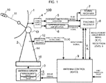
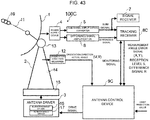
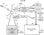
- An antenna system including a control device according to Embodiment 1 of the present invention is described with reference to FIG. 1 to FIG. 4 .
- An antenna system 100 as illustrated in FIG. 1 , mainly includes an antenna 1, an antenna mount 2, an antenna driver 3, a power supply device 4, a sum signal amplification converter 5, a difference signal amplification converter 6, a signal receiver 7, a tracking receiver 8, and an antenna control device 9.
- the antenna 1 receives a radio wave 11 from a moving object 10 such as a satellite or a rocket.
- the antenna mount 2 supports the antenna 1 to be able to change an orientation direction that is a direction in which the antenna 1 is oriented.
- the antenna driver 3 drives the antenna mount 2 thereby changing the orientation direction of the antenna 1.
- the power supply device 4 supplies power to the antenna 1 after amplifying a transmission signal, and generates, based on reception signals received by the antenna 1, a sum signal (SUM) and a difference signal (ERROR) by using the auxiliary power supply system of the power supply device 4.
- the sum signal amplification converter 5 amplifies the sum signal and converts the signal to an intermediate frequency.
- the difference signal amplification converter 6 amplifies the difference signal and converts the signal to the intermediate frequency.
- the signal receiver 7 demodulates the sum signal and acquires data transmitted by the moving object 10.
- the tracking receiver 8 generates, from the sum signal and the difference signal, measurement angle error signals X and Y for driving the antenna mount 2.
- the antenna control device 9 controls the antenna driver 3 such that the antenna 1 is oriented in the arrival direction.
- the arrival direction is a direction from which the radio wave transmitted by the moving object 10 comes and arrives.
- the orientation direction of the antenna 1 is measured by an orientation direction measurer 12.
- the orientation direction of the antenna 1 can be changed by the antenna mount 2.
- the orientation direction is expressed by an azimuth angle and an elevation angle.
- the orientation direction measurer 12 is inputted with signals outputted by angle detection encoders (an encoder for the azimuth angle and an encoder for the elevation angle) that are attached to the antenna 1.
- the orientation direction measurer 12 measures the actual measurement value of the azimuth angle (referred to as the AZ actual angle) of the main beam axis of the antenna 1 based on the signal outputted by the encoder for the azimuth angle, and measures the actual measurement value of the elevation angle (referred to as the EL actual angle) of the main beam axis based on the signal outputted by the encoder for the elevation angle.
- the orientation direction measurer 12 outputs the AZ actual angle and the EL actual angle to the antenna control device 9.
- the orientation direction is represented by a horizon coordinate system based on a combination of (i) an azimuth angle where north is zero degrees and clockwise angles from north are positive and (ii) an elevation angle where directing the horizon is zero degrees.
- the antenna mount 2 includes an elevation angle mount 13, an azimuth angle mount 14, and a base 15.
- the elevation angle mount 13 supports the antenna 1.
- the azimuth angle mount 14 supports the elevation angle mount 13 rotatably around an elevation angle axis (EL-axis) extending horizontally.
- the base 15 supports the azimuth angle mount 14 rotatably around an azimuth angle axis (AZ-axis) extending vertically.
- the azimuth angle may be referred to as an AZ-angle or AZ.
- the EL angle also may be referred to as an EL-angle or EL.
- the antenna control device 9 can be applied also to an X/Y type of antenna mount.
- the antenna driver 3 includes an elevation angle driver 16 and an azimuth angle driver 17.
- the elevation angle driver 16 changes the elevation angle of the elevation angle mount 13 relative to the azimuth angle mount 14.
- the azimuth angle driver 17 changes the azimuth angle of the azimuth angle mount 14 relative to the base 15.
- the elevation angle driver 16 and the azimuth angle driver 17 each have a servo control system.
- the power supply device 4 amplifies a transmission signal of a microwave frequency band to a predetermined power and supplies the amplified power to the antenna 1. Furthermore, the power supply device 4 generates, based on the reception signals received by the antenna 1, a sum signal (SUM) and a difference signal (ERROR) by using the auxiliary power supply system of the power supply device 4.
- the sum signal amplification converter 5 amplifies the sum signal and converts the frequency of the amplified sum signal to a lower frequency.
- the difference signal amplification converter 6 amplifies the difference signal and converts the frequency of the amplified difference signal to the lower frequency.
- the signal receiver 7 processes the sum signal received from the sum signal amplification converter 5 as a modulated communication signal and demodulates the processed signal. The sum signal and the difference signal are inputted to the tracking receiver 8.
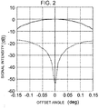
- FIG. 2 is a diagram illustrating an example of changes, with respect to an offset angle, of the sum signal and the difference signal that are generated by the antenna 1 and inputted to the tracking receiver 8.
- the sum signal is represented by a solid line and the difference signal is represented by a dashed line.
- the offset angle is an angle by which the orientation direction changes from a state of directing the moving object 10.
- the offset angle is zero degrees when the orientation direction of the antenna 1 is oriented toward the moving object 10. In a case where the offset angle is zero degrees, the signal intensity of the sum signal is at its highest, whereas the signal intensity of the difference signal is at its lowest.
- the tracking receiver 8 generates, based on the sum signal and the difference signal, measurement angle error signals X and Y for driving the antenna 1, and outputs the measurement angle error signals X and Y to the antenna control device 9.
- the measurement angle error signal X corresponds to an azimuth angle error of the orientation direction
- the measurement angle error signal Y corresponds to an elevation angle error of the orientation direction.
- the antenna control device 9 generates a drive signal for controlling the azimuth angle and the elevation angle of the main beam axis of the antenna 1 and outputs the drive signal to the antenna driver 3.
- the antenna control device 9 controls the azimuth angle and the elevation angle of the main beam of the antenna 1 based on the measurement angle error signals.
- the controlling, based on measurement angle error signals, such that the measurement angle error signals approach zero, is referred to as automatic tracking.
- a method in which the direction of the main beam of the antenna 1 is controlled in accordance with a predetermined change scenario is referred to as program tracking.
- program tracking there is a case where control is performed based on an orbit prediction value, inputted from the external, of the moving object 10 and the change scenario and a case where control is performed only by either the change scenario or the orbit prediction value.
- the orbit prediction value is data representing the position of the moving object 10 per a predetermined width of time.
- the position of the moving object 10 is represented by an azimuth angle and an elevation angle in the direction, on the celestial sphere, of the moving object 10 as viewed from a predetermined observation point.
- the orbit prediction values inputted from the external for example, every second, are interpolated by interpolation calculation to obtain values at a finer time width of 10 msec, for example.
- the antenna control device 9 uses the interpolated orbit prediction values.
- FIG. 3 is a block diagram illustrating the configuration of the tracking receiver.
- the tracking receiver 8, as illustrated in FIG. 3 includes a sum signal AGC circuit 18, a difference signal AGC circuit 19, a 90 degree phase shifter 20, an I-signal detector 21, a Q-signal detector 22, a data storage 23, a coordinate converter 24, and an interface 25.
- AGC is an abbreviation of automatic gain control, that is, automatic amplification ratio control.
- the sum signal AGC circuit 18 is inputted with a sum signal outputted by the antenna 1, the sum signal AGC circuit 18 amplifies the inputted sum signal.
- the amplification ratio of the sum signal AGC circuit 18 changes in accordance with the amplitude of the sum signal.
- the sum signal AGC circuit 18 outputs the amplified sum signal to the 90 degree phase shifter 20 and the I-signal detector 21.
- the sum signal AGC circuit 18 outputs, to the difference signal AGC circuit 19, an amplification voltage.
- the amplification voltage increases in proportion to the increase in the amplification ratio.
- the difference signal AGC circuit 19 is inputted with the difference signal outputted by the antenna 1 and the amplification voltage outputted by the sum signal AGC circuit 18.
- the difference signal AGC circuit 19 changes the amplification ratio in accordance with the value of the amplification voltage inputted from the sum signal AGC circuit 18 and amplifies the inputted difference signal. That is, the difference signal AGC circuit 19 amplifies the inputted difference signal by the amplification ratio that is proportional to the amplification ratio of the sum signal AGC circuit 18. Consequently, the amplified difference signal outputted from the difference signal AGC circuit 19 is amplified by the amplification ratio that is proportional to the amplification ratio of the amplified sum signal outputted from the sum signal AGC circuit 18.
- the difference signal AGC circuit 19 outputs the amplified difference signal to the I-signal detector 21 and the Q-signal detector 22.
- the 90 degree phase shifter 20 shifts (changes) the phase of the amplified sum signal outputted from the sum signal AGC circuit 18 by 90 degrees.
- the 90 degree phase shifter 20 outputs, to the Q-signal detector 22, the amplified sum signal with phase shifted by 90 degrees.
- the shifting of the phase by 90 degrees means that the phase is increased by 90 degrees.
- the I-signal detector 21 detects the difference signal that is outputted from the difference signal AGC circuit 19 by the sum signal (sum signal without phase shifting) that is outputted from the sum signal AGC circuit 18. In other words, the I-signal detector 21 outputs a product of the sum signal outputted from the sum signal AGC circuit 18 and the difference signal outputted from the difference signal AGC circuit 19. The I-signal detector 21 outputs the detected signal (hereinafter referred to as the "I-signal") to the coordinate converter 24.
- the axis where the I-signal is detected is referred to as the I-axis.
- the Q-signal detector 22 detects the difference signal outputted from the difference signal AGC circuit 19 by the sum signal outputted from the 90 degree phase shifter 20. In other words, the Q-signal detector 22 outputs the product of the sum signal outputted from the 90 degree phase shifter 20 and the difference signal outputted from the difference signal AGC circuit 19. The Q-signal detector 22 outputs the detected signal (hereinafter referred to as the "Q-signal") to the coordinate converter 24.
- the axis where the Q-signal is detected is referred to as the Q-axis.
- the phase correction value 51 and the sensitivity coefficient 52 used by the coordinate converter 24 are stored in the data storage 23.
- the phase correction value 51 and the sensitivity coefficient 52 are calculated by the antenna control device 9.
- the phase correction value 51 is a correction value by which the phase of the I-axis and the Q-axis are corrected.
- the I-axis where the measurement angle error signal X is detected aligns with a U-axis (described later) that corresponds to the azimuth angle of the orientation direction
- the Q-axis where the measurement angle error signal Y is detected aligns with a V-axis (described later) that corresponds to the elevation angle of the orientation direction.
- the sensitivity coefficient 52 is a factor of proportionality between the magnitude of the measurement angle error signal and the absolute value of the error of the orientation direction.
- the coordinate converter 24 uses the phase correction value 51 and the sensitivity coefficient 52 to perform coordinate conversion on the I-signal and the Q-signal and then outputs the measurement angle error signals X and Y. Coordinate conversion is described later.
- the measurement angle error signals X and Y are outputted by the tracking receiver 8.
- the signal intensity (reception level) of the sum signal inputted to the sum signal AGC circuit 18 is also outputted by the tracking receiver 8.
- the measurement angle error signal is an arrival direction error representing the difference between the arrival direction and the orientation direction of the antenna 1.
- the arrival direction is the direction from which the radio wave 11 comes and arrives.
- the measurement angle error signal is generated from the sum signal and the difference signal of the reception signals.
- the tracking receiver 8 is a measurement angle processor that is inputted with the sum signal and the difference signal of the reception signals and calculates an arrival direction error.
- the interface 25 receives, from the antenna control device 9, a monitoring signal indicating whether or not the antenna control device 9 is operating normally.
- the interface 25 transmits, to the antenna control device 9, a monitoring signal indicating whether or not the tracking receiver 8 is operating normally. Transmission/reception of data such as the phase correction value y and sensitivity coefficient K and control signals between the tracking receiver 8 and the antenna control device 9 is also performed.
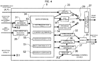
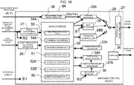
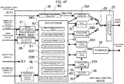
- FIG. 4 is a block diagram illustrating the configuration of the antenna control device according to Embodiment 1.
- the antenna control device 9 includes an orbit prediction value data generator 26, an antenna drive controller 27, a program controller 28, a toggle switch 29, a mode determiner 30, an error measurement data generator 31, a correction value calculator 32, a tracking controller 33, a data storage 34, an interface 35, an oscillation detector 36, an oscillation cause determiner 37, and a correction value updater 38.
- the orbit prediction value data generator 26 generates orbit prediction value data 53 obtained by performing interpolation calculation of orbit prediction values inputted externally every second, for example, to obtain values at a finer time width of 10 msec, for example. Then, the orbit prediction value data generator 26 stores the generated orbit prediction value data 53 into the data storage 34.
- the antenna drive controller 27 generates a drive signal that drives the antenna driver 3 such that the difference between the command value being inputted and the direction orientation direction of the antenna 1 approaches zero.
- the antenna drive controller 27 amplifies the power of the drive signal to a level necessary for the antenna driver 3.
- the program controller 28 generates a command value based on the orbit prediction value data 53 and the change scenario 54 and outputs the generated command value to the antenna drive controller 9.
- An example of the change scenario 54 is illustrated in FIG. 5 .
- the change scenario 54 indicates a time transition of orientation operation amount by which the orientation direction is changed from the orbit prediction value that is indicated by the orbit prediction value data 53.
- the term "orientation operation amount" is the amount by which the orientation direction is changed from the orbit prediction value.
- the program controller 28 outputs, as the command value, an orientation direction obtained by adding the orientation operation amount indicated in the change scenario 54 to the predicted position of the moving object 10 every control time based on the orbit prediction value data 53.
- the toggle switch 29 switches between program tracking and automatic tracking.
- the antenna drive controller 27 is inputted with the command value outputted by the program controller 28.
- the toggle switch 29 is on the automatic tracking side
- the antenna drive controller 27 is inputted with the command value calculated by the tracking controller 33.
- the state during which the antenna drive controller 27 is inputted with the command value outputted by the tracking controller 33 is referred to as "the tracking controller 33 is in operation” and the state during which the antenna drive controller 27 is inputted with the command value outputted by the program controller 28 is referred to as "program controller 28 is in operation”.
- the mode determiner 30 determines whether to operate in program tracking mode or automatic tracking mode. If the mode determiner 30 determines that it is necessary to change the mode, the mode determiner 30 changes the mode toggle switch 29 to the side to be used. The mode switching between program tracking and automatic tracking can be changed also through an instruction given by a user.
- the error measurement data generator 31 generates error measurement data 55 while the program controller 28 is in operation.
- the error measurement data 55 contains an AZ actual angle and an EL actual angle measured by the orientation direction measurer 12 and measurement angle error signals outputted by the tracking receiver 8, all of which are measured at the time of the command value of the same orientation direction.
- the error measurement data 55 contains the measurement angle error signals X and Y and the AZ actual angle and the EL actual angle being actual measurement values of the orientation direction when the reception signals (sum signal and difference signal), from which the measurement angle error signals are obtained, are inputted.
- the generated error measurement data 55 is stored in the data storage 34.
- the correction value calculator 32 calculates, based on at least three pieces of the error measurement data 55, a correction parameter that can correct the measurement angle error signals and make the difference between the orientation direction of the antenna 1 and the arrival direction approach zero.
- the error measurement data 55 for each of the at least three pieces are generated at conditions in which the program controller 28 outputs the command values that are different each other.
- the correction parameters to be calculated are the phase correction value 51 that is an angle by which the measurement angle error signal is rotated, and the sensitivity coefficient 52 by which the measurement angle error signal is multiplied.
- the calculated phase correction value 51 and the sensitivity coefficient 52 are stored in the data storage 23 included in the tracking receiver 8 and into the data storage 34. The method by which the correction value calculator 32 calculates the phase correction value 51 and the sensitivity coefficient 52 is described later.
- the tracking controller 33 calculates command value obtained by adding the measurement angle error signal and the change caused by the orbit prediction value to the orientation direction actual measurement value. In a case where an orbit prediction value of the communication counterpart does not exist, the change caused by the orbit prediction value is set to zero.
- the interface 35 receives, from the tracking receiver 8, a monitoring signal indicating whether or not the tracking receiver 8 is operating normally.
- the interface 35 transmits, to the tracking receiver 8, the monitoring signal indicating whether or not the antenna control device 9 is operating normally. Also, the transmission/reception of data such as the phase correction value ⁇ and sensitivity coefficient K and control signals between the tracking receiver 8 and the antenna control device 9 is also performed.
- the oscillation detector 36 detects oscillation. Oscillation is a phenomenon where the orientation direction of the antenna 1 periodically changes during automatic tracking. FIG. 14 and FIG. 16 illustrate examples where oscillation is occurring.
- the oscillation detector 36 checks the orientation direction actual measurement values within, for example, a predetermined length of time, and detects oscillations in a case where there is a fluctuation greater than or equal to a predetermined threshold.
- the oscillation cause determiner 37 activates the error measurement data generator 31 and the correction value calculator 32 multiple times.
- the oscillation cause determiner 37 determines the cause of the oscillation based on multiple phase correction values ⁇ and sensitivity coefficients K.
- the oscillation cause determiner 37 determines a phase shift in which the phase of the measurement angle error signal has changed or a sensitivity shift in which the sensitivity coefficient has changed as being the cause of the oscillation.
- the oscillation detector 36 may not be provided in a case where, during automatic tracking, the error measurement data generator 31 and the correction value calculator 32 are always operated periodically.
- the correction value updater 38 updates the phase correction value ⁇ .
- the correction value updater 38 updates the sensitivity coefficient K.
- the updated phase correction value ⁇ new and the sensitivity coefficient Knew are stored in the data storage 23 of the tracking receiver 8 and the data storage 33.
- the newly calculated phase correction value ⁇ now is determined based on at least one piece of ⁇ among the phase correction values ⁇ calculated at and after the time when oscillation is detected. In the case where ⁇ now is determined based on multiple pieces of ⁇ , the phase correction value ⁇ now is determined by use of an appropriate method such as the averaging or median operation.
- the phase correction values ⁇ calculated at and after the time when oscillation is detected are union of the ⁇ calculated for determining the cause of oscillation and the ⁇ calculated after identifying the cause of oscillation.
- the newly calculated sensitivity coefficient Know is determined based on at least one piece of K among the sensitivity coefficients K calculated at and after the time when oscillation is detected. In the case where Know is determined based on multiple pieces of K, the newly calculated sensitivity coefficient Know is determined by use of an appropriate method such as the averaging or median operation.
- the sensitivity coefficients K calculated at and after the time when oscillation is detected are union of the K calculated for determining the cause of oscillation and the K calculated after identifying the cause of oscillation.
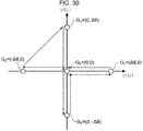
- FIG. 5 is a diagram illustrating an example of a trajectory in which an orientation direction is changed when program tracking is performed by the antenna control device according to Embodiment 1.
- the trajectory that changes by the orbit prediction value is represented by one point G o on the celestial sphere defined in the horizontal coordinate system.
- G o is referred to as the reference celestial sphere point.
- the celestial sphere point G o is the prediction direction being the orientation direction predicted based on the orbit prediction value.
- the reference celestial sphere point is (i) an orientation direction of the orbit prediction value at one time point determined appropriately in a determined change scenario 54, such as the starting point, an intermediate point, or an end point of the change scenario 54 or (ii) a centroid of the orbit prediction values during a time period.
- the celestial sphere points and the reference celestial sphere point G o that are used to create the error measurement data 55 are denoted by white circles.
- the vertical direction shown in the figure is referred to as the V-direction.
- the V-direction is the direction of the great circle on the celestial sphere in which the elevation angle changes.
- the direction of the great circle that is perpendicular to the V-direction on the celestial sphere is referred to as the U-direction.
- the U-direction is the horizontal direction in the figure. Since the trajectory on the celestial sphere in which the azimuth angle changes while the elevation angle is constant is a small circle, strictly speaking, the trajectory differs from the U-direction.
- the difference between (i) the trajectory on the celestial sphere in which the azimuth angle changes in a range with minute changes and (ii) the U-direction can be ignored.
- the great circle of the U-direction which passes on the reference celestial sphere point is referred to as the U-axis.
- the great circle of the V-direction which passes on the reference celestial sphere point is referred to as the V-axis.
- the offset angle is ⁇
- the frequency of the rotation of the program command value is f
- the angular velocity 2 ⁇ f
- the time elapsed from the start of the change scenario 54 is t.
- the offset angle ⁇ is the reference angle used for changing an orientation direction.
- Equation (3) and Equation (4) mean that the program command value ( ⁇ u, ⁇ v), which is the command value of the orientation direction, is calculated such that the angular difference from reference celestial sphere point G o is in a range within the offset angle ⁇ .
- the offset angle ⁇ is a predetermined maximum angle difference relative to the angular difference between the reference celestial sphere point G o and the command value of the orientation direction.
- the program command value moves so that its trajectory forms a circle on the celestial sphere, the circle has a center located at G 0 and a radius ⁇ .
- the ⁇ is a small value that is less than or equal to approximately 1/10 of the half width of the antenna 1.
- the drop in the reception level when circular movement is made in accordance with the program command value is less than approximately 0.3 dB including the control response error of the antenna 1.
- the error measurement data 55 is created during program tracking based on ten or more celestial sphere points G j .
- the command value represented by a pair of the azimuth angle and the elevation angle are inputted.
- the command value of the azimuth angle and the elevation angle corresponding to the celestial sphere point G assumed to be (AZ0(t), EL0(t)), is expressed as follows.
- the frequency f is set to approximately 1 Hz, and the time during which the orientation direction of the antenna device 1 changes becomes short. Also, in a case where the phase calculation accuracy is low because the antenna device 1 being unable to maintain proper tracking at 1 Hz due to the frequency band characteristics of the antenna servo loop, the frequency may be decreased to less than 1 Hz in accordance with the frequency band characteristics of the servo loop.
- the command value of the orientation direction may be changed using a movement other than circular movement, for example, square-like movement and grid-like movement.
- the offset angle ⁇ is a change reference angle used as a reference for changing the command value in a change scenario.
- the change range of the command value is proportional to the offset angle ⁇ .
- the maximum angle difference being the maximum value of the angle differences from the reference celestial sphere points of command values that change by the change scenario, is determined by the offset angle ⁇ .
- the orientation direction is expressed by the U-axis and V-axis coordinate system with the reference celestial sphere point G o being the origin.
- the U-axis component of the orientation direction is referred to as the U-angle whereas the V-axis component of the orientation direction is referred to as the V-angle.
- G j j-th program command value.
- Puj U-angle of G j .
- Pvj V-angle of G j .
- Uj U-angle of the actual measurement value of the orientation direction at the time of being G j .
- Vj V-angle of the actual measurement value of the orientation direction at the time of being G j .
- Hj Point on the celestial sphere representing the actual measurement value of the orientation direction at the time of being G j .
- Hj (Uj, Vj).
- Xj Measurement angle error signal X obtained from the sum signal and the difference signal at the time of being G j .
- Yj Measurement angle error signal Y obtained from the sum signal and the difference signal at the time of being G j .
- Vsj Measurement angle error vector represented by the measurement angle error signals X and Y at the time of being G j .
- Vsj (Xj, Yj).
- P 0 Arrival direction.
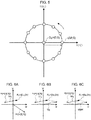
- FIGS. 6A, 6B, and 6C illustrate the process for correcting a measurement angle error victory based on a phase correction value and a sensitivity coefficient calculated by the antenna control device according to Embodiment 1.
- FIGS. 6A, 6B, and 6C illustrate the variables at the time of the program correction value G j .
- FIG. 6A illustrates the actual measurement value Hj of the orientation direction, the arrival direction P 0 , the actual measurement value error vector Vhj of the arrival direction that is determined based on the actual measurement value Hj, and the measurement angle error vector Vsj that is obtained from the sum signal and the difference signal.
- FIG. 6B illustrates the vector Vgj where Vsj is rotated by the phase correction value ⁇ . Vhj and Vgj direct in the same direction.
- FIG. 6C illustrated a case where Vgj is multiplied by the sensitivity coefficient K. The direction and magnitude of Vhj and Vgj/K are the same.
- the coordinate converter 24 uses the phase correction value ⁇ and the sensitivity coefficient K to perform coordinate conversion and then outputs the measurement angle error signals X and Y.
- the measurement angle error signals before correction are represented by the variables Xb and Yb.
- X Y 1 K cos ⁇ ⁇ sin ⁇ sin ⁇ cos ⁇ Xb Yb
- Equation (13) K ⁇ X 1 ⁇ X 2 ⁇ sin ⁇ + Y 1 ⁇ Y 2 ⁇ cos ⁇
- Equation (14) and Equation (15) are each squared and then added together.
- U 2 ⁇ U 1 2 + V 2 ⁇ V 1 2 K 2 ⁇ X 1 ⁇ X 2 2 + Y 1 ⁇ Y 2 2
- Equation (16) is modified by Lh and Ls, the equation for calculating K is as follows.
- Equation (22) and Equation (23) can be expressed as follows.
- the correction value calculator 32 uses error measurement data 55 generated by the program command value G j of N pieces (at least three pieces), and can calculate the phase correction value ⁇ and the sensitivity coefficient K with reduced influence of noise. Additionally, the variables shown below are defined.
- Xfj Measurement angle error signal X after correction by the assumed Du, Dv, ⁇ , and K.
- Yfj Measurement angle error signal Y after correction by the assumed Du, Dv, ⁇ , and K.
- Xfj and Yfj can be calculated using the following equations.
- Xfj Yfj K cos ⁇ sin ⁇ ⁇ sin ⁇ cos ⁇ Du ⁇ Uj Dv ⁇ Vj
- Du ⁇ Uj Dv ⁇ Vj 1 K cos ⁇ ⁇ sin ⁇ sin ⁇ cos ⁇ Xfj Yfj
- the correction value calculator 32 determines ⁇ and K such that the following error function E is minimized.
- E ⁇ Xj ⁇ Xfj 2 + Yj ⁇ Yfj 2
- the error function E is the sum of squares of post-correction residuals for N pieces of the error measurement data 55.
- Each of the post-correction residuals is the difference between (i) the arrival direction error (Xfj, Yfj) obtained by correcting the actual measurement value error (Du -Uj, Dv - Vj) by using the correction parameters including the phase correction value and (ii) the arrival direction error (Xj, Yj) inputted from the tracking receiver 8.
- Equation (30) ⁇ Xj 2 + Yj 2 ⁇ 2 ⁇ K ⁇ ⁇ Du ⁇ Uj ⁇ Xj ⁇ cos ⁇ ⁇ Yj ⁇ sin ⁇ ⁇ 2 ⁇ K ⁇ ⁇ Dv ⁇ Vj ⁇ Xj ⁇ sin ⁇ + Yj ⁇ cos ⁇ + K 2 ⁇ ⁇ Du ⁇ Uj 2 + Dv ⁇ Vj 2
- Equation (31) becomes the following.
- E N ⁇ xs 0 + ys 0 ⁇ 2 N ⁇ K ⁇ Du ⁇ u 0 ⁇ x 0 ⁇ cos ⁇ ⁇ y 0 ⁇ sin ⁇ + d 0 ⁇ cos ⁇ ⁇ e 0 ⁇ sin ⁇ ⁇ 2 N ⁇ K ⁇ Dv ⁇ v 0 ⁇ x 0 ⁇ sin ⁇ + y 0 ⁇ cos ⁇ + f 0 ⁇ sin ⁇ + g 0 ⁇ cos ⁇ + N ⁇ K 2 ⁇ Du ⁇ u 0 2 + Du ⁇ v 0 2 + us 0 + vs 0
- ⁇ tan ⁇ 1 f 0 ⁇ e 0 / d 0 + g 0
- K ⁇ d 0 + g 0 2 + f 0 ⁇ e 0 2 / us 0 + vs 0
- this method has a feature that enables to calculate the prediction value errors (Du, Dv) even when there is a deviation between the orbit prediction value and the satellite position, and enables to calculate the phase correction value ⁇ and the sensitivity coefficient K that are not influenced with the forecast value errors.
- the post-correction values with respect to Uj and Vj may be calculated as follows.
- Ufj post-correction value of Uj calculated using the assumed Du
- Vfj post-correction value of Vj calculated using the assumed Du, Dv, ⁇ , and K
- the phase correction value ⁇ and the sensitivity coefficient K are calculated by minimizing the error function E2 that is represented by Ufj and Vfj.
- E 2 K 2 ⁇ ⁇ Ufj ⁇ Uj 2 + Vfj ⁇ Vj 2
- the error function E2 is the sum of squares of post-correction residuals for N pieces of the error measurement data 55.
- Each of the post-correction residuals is the difference between (i) the actual measurement value error (Du - Ufj, Dv - Vfj) obtained by correcting the arrival direction error with the correction parameters including the phase correction value ⁇ and (ii) the actual measurement value error (Du - Uj, Dv - Vj).
- the error function E2 is the same as the error function E. Even in a case where the error function E2 is minimized, the phase correction value ⁇ and the sensitivity coefficient K can be calculated to be the same value as that calculated when the error function E is minimized.
- phase correction value ⁇ and the sensitivity coefficient K calculated by the correction value calculator 32 are stored in the data storage 23 included in the tracking receiver 8 and into the data storage 34.
- the values that are stored are not the calculated values without further processing. Rather, as illustrated in Equation (1) and Equation (2), the values set before updating are corrected and set.
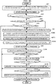
- FIG. 7 is a flowchart illustrating a procedure for tracking the moving object by the antenna control device according to Embodiment 1.
- step S01 information such as the reception frequency and the orbit prediction value are set depending on the moving object 10 to be tracked being a satellite or others.
- step S02 program tracking starts.
- the mode determiner 30 sets the toggle switch 29 to the program tracking side.
- step S03 the mode determiner 30 checks whether a reception level S outputted by the tracking receiver 8 is greater than or equal to a lower limit value Smin. If the reception level S is greater than or equal to the lower limit value Smin (YES in S03), the radio wave 11 from the moving object 10 is considered to be captured, and thus processing proceeds to step S04. If the reception level S is less than the lower limit value Smin (No in S03), S03 is repeated at a predetermined interval.
- step S04 a check is performed as to whether the parameter for phase adjustment is set to the value indicating that phase adjustment is executed in every tracking. If phase adjustment is not to be executed in every tracking, a check is performed, in step S05, as to whether the phase correction value y and so on for the frequency used for present tracking, had been calculated. If phase adjustment is executed in every tracking in S04 or if calculation is not finished in step S05, step S06 is performed.
- the program controller 28 outputs the command value of the orientation direction of the antenna device 1 to change in accordance with a predetermined change scenario. While the orientation direction changes in accordance with the change scenario, the error measurement data generator 31, at a predetermined time interval, generates error measurement data 55 and stores into the data storage 34.
- step S07 the correction value calculator 32 calculates the phase correction value ⁇ and the sensitivity coefficient K and stores them into the data storage 34.
- a change scenario 54 is performed and a phase correction value ⁇ and a sensitivity coefficient K are calculated.
- the program controller 28 changes the command value of the orientation direction in accordance with the change scenario 54 and generates error measurement data 55 for three or more pieces.
- the phase correction value ⁇ and the sensitivity coefficient K are calculated based on the generated error measurement data 55.
- the moving object 10 is supposed to be an artificial satellite orbiting at the orbit altitude of 500 Km.
- the elevation angle is approximately 5 degrees.
- the noise superimposed on the measurement angle error signal is approximated using a Gauss random number and the effective value of that magnitude is set to be 0.003° rms (root mean square).
- the noise superimposed on the actual measurement value of the orientation direction of the antenna 1 is approximated using a Gauss random number and that magnitude is set to be 0.003° rms.
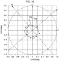
- the first example is illustrated in FIG. 8 to FIG. 10 .
- the simulation conditions are as follows.
- Phase correction value ⁇ 40° Sensitivity coefficient
- K 1 U-direction prediction value error
- Du 0°
- Dv 0°
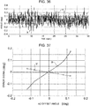
- FIG. 8 illustrates a trajectory of actual measurement values Hj of the orientation direction of the antenna 1 and a trajectory of the measurement angle error vectors Vsj calculated from the sum signal and the difference signal in a case where the orbit prediction values are represented by a single point on the celestial sphere .
- the orientation direction actual measurement value Hj is denoted by a solid line with white circles.
- the measurement angle error vector Vsj is denoted by a dashed-line with white rhombuses.
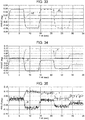
- FIGS. 9A, 9B, 9C, 9D, and 9E are diagrams illustrating temporal changes of measurement data in the case of FIG. 8 .
- the orientation direction is changed between 2 seconds and 3 seconds from the start of the simulation.
- FIG. 9A illustrates temporal changes of an azimuth angle actual measurement value 81 and an azimuth angle servo system tracking error 82.
- FIG. 9B illustrates temporal changes of an elevation angle actual measurement value 83 and an elevation angle servo system tracking error 84.
- FIG. 9C illustrates temporal changes of the signal intensity of the sum signal.
- FIG. 9D illustrates temporal changes of the azimuth angle actual measurement value Uj and the azimuth angle measurement angle error signal Xj.
- FIG. 9E illustrates temporal changes of the elevation angle actual measurement value Vj and the measurement angle error signal Yj.
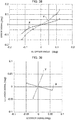
- the trajectory of the post-correction measurement angle error vector Vaj corrected based on the measurement angle vector Vsj by using ⁇ , K, Du, and Dv and the trajectory of the measurement angle error vector Vsj are illustrated in FIG. 10 .
- the post-correction measurement angle error vector Vaj is denoted by a dash-dot line with black triangles.
- the actual measurement value Hj of the orientation direction is not shown for ease in viewing this figure.
- FIG. 11 to FIG. 13 The second example is illustrated in FIG. 11 to FIG. 13 .
- the simulation conditions are as follows.
- FIG. 11 to FIG. 13 are expressed in a manner similar to that in FIG. 8 to 10 .
- FIG. 13 also illustrates the actual measurement value Hj of the orientation direction.
- Phase correction value ⁇ 40°
- V-direction prediction value error Dv 0.03°
- step S10 the tracking controller 33 calculates command value obtained by adding the measurement angle error signals X and Y to the orbit prediction value and then outputs the command value to the antenna drive controller 27.
- the oscillation detector 36 checks periodically in step S11 whether or not automatic tracking is oscillating.
- Oscillation refers to a phenomenon where the orientation direction changes periodically as illustrated in FIG. 14 and FIG. 16 .
- the difference between the orbit prediction value and the orientation direction actual measurement value with respect to the azimuth angle or the elevation angle is greater than or equal to a predetermined threshold, it is determined that there is oscillation.
- Other methods may be used for detecting oscillation. Any method may be used as a method for detecting oscillation, as long as the method can determine that the azimuth angle or the elevation angle fluctuates with respect to an orbit prediction value.
- the oscillation cause determiner 37 activates the error measurement data generator 31 and the correction value calculator 32 multiple times to calculate multiple pieces of the phase correction value ⁇ and the sensitivity coefficient K.
- step S13 a check is performed as to whether or not phase shift is the cause of the oscillation.
- Phase shift is a state in which the phase correction cannot be accurately performed using the phase correction value ⁇ , because phase of the measurement angle signal is shifted and causes oscillation.
- a condition for determining that the oscillation is caused by phase shift is, for example, a condition in which the multiple calculated phase correction values y are within range not including zero degrees and having a predetermined width.
- the oscillation cause determiner 37 is a phase shift detector that determines that phase shift is occurring when multiple calculated phase correction values ⁇ calculated while the tracking controller is in operation are within range not including zero degrees and having the predetermined width.
- the multiple calculated phase correction values ⁇ are within the range not including zero degrees and having the predetermined width, it is determined that oscillation is occurring due to phase shift. In a case where the multiple calculated phase correction values are within a predetermined range including zero degrees, it is understood that phase correction value ⁇ is not shifted. Also, in a case where the phase correction value ⁇ fluctuates beyond the predetermined width, it can be considered that oscillation is occurring due to another factor and that the phase correction value ⁇ is fluctuating under the influence of the oscillation.
- the correction value updater 38 in step S14, updates the phase correction value ⁇ as illustrated in Equation (1), and stores the phase correction value ⁇ new into the data storage 34 and the data storage 23.
- the correction value updater 38 is a phase correction value updater that updates the phase correction value when the oscillation cause determiner 37 detects phase shift.
- step S15 a check is performed as to whether or not the oscillation is caused by sensitivity shift.
- Sensitivity shift is a state in which correction cannot be accurately performed using the sensitivity coefficient K due to the shift in the sensitivity coefficient of the measurement angle error signal.
- a condition for determining that the oscillation is caused by sensitivity shift is, for example, a condition in which multiple calculated sensitivity coefficients K are within a range not including 1 and having a predetermined width. In the case where the multiple calculated sensitivity coefficients K are within a predetermined range not including 1, it is determined that oscillation is occurring due to sensitivity shift.
- the oscillation cause determiner 37 is a sensitivity shift detector that detects sensitivity shift when multiple sensitivity coefficients K calculated while the tracking controller is in operation are within range not including 1 and having the predetermined width.
- the correction value updater 38 in step S16, updates the sensitivity coefficient K as illustrated in Equation (2), and stores the sensitivity coefficient Knew into the data storage 34 and the data storage 23.
- the correction value updater 38 is a sensitivity coefficient updater that updates the sensitivity coefficient when the oscillation cause determiner 37 detects sensitivity shift.
- step S17 If it is not determined that the oscillation is caused by sensitivity shift NO in S15), the cause is unknown, and thus the mode is changed to program tracking in step S17.
- An impact on the communication quality caused by a deviation between the moving object 10 and the orientation direction during program tracking depends on the accuracy of the orbit prediction value and the orientation accuracy inherent to the antenna 1.
- the communication quality can be determined on the basis of, for example, whether a bit error rate generated by the signal receiver 7 satisfies a requirement criterion.
- the saved correction parameter may be used to resume automatic tracking. If the saved correction parameter is used, the saved correction parameter is set in the data storage 34 and the data storage 23. If the moving object 10 is captured, the toggle switch 29 switches to the automatic tracking side.
- FIG. 14 and FIGS. 15A and 15B illustrate the simulation results in the case where oscillation occurred due to phase shift.
- FIG. 14 is a diagram illustrating temporal changes of actual measurement values of the azimuth angle and the elevation angle.
- the solid line with black dots denotes the azimuth angle (AZ) and the dash-dot line with white triangles denotes the elevation angle (EL).
- FIGS. 15A and 15B illustrate temporal changes of the phase correction value ⁇ and the sensitivity coefficient K.
- FIG. 15A illustrates temporal changes of the phase correction value ⁇ .
- FIG. 15B illustrates temporal changes of the sensitivity coefficient K.
- the solid line with the black dots denotes the phase correction value ⁇ and the sensitivity coefficient K that are corrected in the present invention.
- the dashed line with white diamonds denotes the phase correction value ⁇ w and the sensitivity coefficient Kw that are calculated by that in Patent Literature 3.
- the phase correction value ⁇ can be calculated from 5.9 seconds.
- the method of Patent Literature 3 can calculate the phase correction value ⁇ w from 5 seconds.
- the phase correction value ⁇ fluctuates less than the phase correction value ⁇ w, and it can be recognized that the phase correction value ⁇ can be calculated more accurately. If the predetermined width at which the phase correction value ⁇ is determined to be fluctuating is 5 degrees, it can be determined that the phase correction value ⁇ is not fluctuating. However, the phase correction value ⁇ w calculated using the method of Patent Literature 3 is determined to be fluctuating.
- the sensitivity coefficient K fluctuates somewhat more than the sensitivity coefficient Kw.
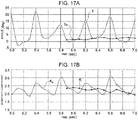
- FIG. 16 and FIGS. 17A and 17B illustrate the simulation results in a case where oscillation occurred due to the shift in sensitivity coefficient K.
- FIG. 16 is similar to FIG. 14 .
- FIGS. 17A and 17B illustrated temporal changes of the phase correction value ⁇ and the sensitivity coefficient K.
- FIG. 17A is a diagram illustrating temporal changes of the phase correction value.
- FIG. 17B is a diagram illustrating temporal changes of the sensitivity coefficient K.
- the phase correction value ⁇ fluctuates less than the phase correction value ⁇ w, and it can be recognized that the phase correction value ⁇ can be calculated more accurately.
- the sensitivity coefficient K also fluctuates less than the sensitivity coefficient Kw.
- phase correction value ⁇ For the phase correction value ⁇ , all of the calculated phase correction values ⁇ are within a 5 degree range including 0 degrees. It is not determined that the phase correction value ⁇ is shifted. The phase correction value ⁇ w is fluctuating by over 20 degrees. In a case where the phase correction value ⁇ w is used, it is not determined that there is oscillation caused by the shift of the phase correction value ⁇ w.
- the sensitivity coefficient K is in a range from approximately 2.0 to approximately 2.5.
- the sensitivity coefficient Kw caused by the method of Patent Literature 3 is in a range of approximately 1.9 to approximately 3.0.
- a term referred to as the fluctuation width indicates the ratio of the largest value of the calculated sensitivity coefficients divided by the smallest value of the calculated sensitivity coefficients. If it is determined that the sensitivity coefficient K is fluctuating on the condition of the fluctuation width being, for example, greater than or at 130%, it can be determined that the sensitivity coefficient is not fluctuating.
- the threshold with respect to the fluctuation width such as 130% is determined in advance.
- the sensitivity coefficient Kw calculated using the method in Patent Literature 3 is determined to be fluctuating.
- the fluctuation width may be a value obtained by dividing the largest value of the calculated sensitivity coefficients by an average value of the calculated sensitivity coefficients. Alternatively, the value may be obtained by dividing the average value of the calculated sensitivity coefficients by the smallest value of the calculated sensitivity coefficients.
- the fluctuation width may be calculated any way as long as the magnitude of fluctuation of the sensitivity coefficients can be expressed.
- the phase adjustment and sensitivity adjustment can be automatically performed before the starting of tracking of the moving object. Therefore, erroneous operation due to human error can be prevented and work efficiency can be enhanced.
- the present invention provides more accurate calculation of the phase correction value and the sensitivity coefficient than method described in Patent Literature 3 even in a case where the signal-to-noise ratio of the difference signal is low.
- it can be determined whether the oscillation is caused by phase shift or sensitivity shift, and if the cause is phase shift, the oscillation can be eliminated by updating the phase correction value. If the cause is sensitivity shift, the oscillation can be eliminated by updating the sensitivity coefficient.
- the phase correction value and the sensitivity coefficient can be calculated accurately even when the signal-to-noise ratio of the difference signal is low, the measurement angle error signals can be calculated more accurately than conventional methods, and thus the communication counterpart can be tracked accurately.
- phase correction value ⁇ and the sensitivity coefficient K are both calculated, only the phase correction value ⁇ may be calculated. In the case where only the phase correction value ⁇ is calculated, a predetermined value or a value of 1 is used for the sensitivity coefficient K.
- the error function E is a sum of squares of post-correction residuals for N pieces of the error measurement data.
- Each of the post-correction residuals used in the error function E is the difference between the arrival direction error and the actual measurement value error corrected based on the phase correction value and the sensitivity coefficient.
- the error function E2 is the sum of squares of post-correction residuals for N pieces of the error measurement data.
- Each of the post-correction residuals used in the error function E2 is the difference between the actual measurement value error and the arrival direction error corrected based on the phase correction value and the sensitivity coefficient.
- the phase correction value and the sensitivity coefficient may be obtained by correcting one of the actual measurement value error and the arrival direction error by each of the phase correction value and the sensitivity coefficient, and by minimizing the sum of squares of post-correction residuals for N pieces of the error measurement data.
- An example of correcting one of the actual measurement value error and the arrival direction error by each of the phase correction value and the sensitivity coefficient is a case where the actual measurement value error is corrected based on the phase correction value, and the arrival direction error is corrected based on the sensitivity coefficient.
- a correction parameter other than the phase correction value and the sensitivity coefficient may be used for performing the correction.
- additional correction parameters include orthogonality and the sensitivity coefficient set as having different values for the azimuth angle direction and the elevation angle direction. Orthogonality expresses degree of a difference from 90 degrees the phase difference between the I-axis and the Q-axis that are used for generating the measurement angle error signals X and Y from the sum signal and the difference signal.
- Embodiment 2 is obtained by modifying Embodiment 1 such that a case where detection axes used for performing quadrature detection on the measurement angle error signals X and Y is not orthogonal is taken into account and a case where the sensitivity coefficient is set to be different for AZ and EL is also taken into account. Also, the coordinate converter 24 of the tracking receiver 8 is set such that substantially no coordinate conversion is performed. A tracking receiver that is not equipped with a coordinate converter is also applicable to Embodiment 2.
- FIG. 18 is a diagram illustrating a configuration of an antenna system including an antenna control device according to Embodiment 2 of the present invention.
- FIG. 19 is a block diagram illustrating a configuration of the antenna control device according to Embodiment 2.
- An antenna control device 9A that is included in an antenna system 100A additionally includes a measurement angle error corrector 39, and a correction value calculator 32A, a tracking controller 33A, and a data storage 34A are modified.
- the measurement angle error corrector 39 performs corrections to the measurement angle error signals, which is performed by the coordinate converter 24 included in the tracking receiver 8. Therefore, the phase correction value ⁇ is set to zero degrees and the sensitivity coefficient K is set to 1 in the data storage 23 included in the tracking receiver 8. By setting the values in this manner, it can be made equivalent to the case in which the coordinate converter 24 do nothing. Thus, it is unnecessary for the antenna control device 9A to set and change the phase correction value ⁇ and the sensitivity coefficient K in the data storage 23. In a case where the coordinate converter 24 can perform the same conversion as the measurement angle error corrector 39, the data is stored in the data storage 23 and the coordinate converter 24 can perform the conversion using the data stored in the data storage 23. Also, in this case, the antenna control device 7A may not be equipped with the measurement angle error corrector 39.
- the data storage 34A stores an AZ sensitivity coefficient 52A and an EL sensitivity coefficient 52B instead of storing the sensitivity coefficient 52 and also stores the orthogonality 56.
- the AZ sensitivity coefficient 52A is an azimuth angle sensitivity coefficient that is a sensitivity coefficient for the azimuth angle direction.
- the EL sensitivity coefficient 52B is an elevation sensitivity coefficient that is a sensitivity coefficient for the elevation angle direction.
- the orthogonality 56 expresses degree of a difference from 90 degrees the phase difference between the I-axis and the Q-axis that are used for generating the measurement angle error signals X and Y from the sum signal and the difference signal.
- the orthogonality 56 expresses the difference between (i) the angle between the I-axis and the Q-axis that are two axes where quadrature detection is performed on the measurement angle error signals X and Y and (ii) 90 degrees.
- the radiation pattern of the main lobe of the radio wave that is received by the antenna 1 can be expressed also in a case where the radiation pattern is determined by parameters having different values for azimuth angle and elevation angle.
- the AZ sensitivity coefficient 52A, the EL sensitivity coefficient 52B, and the variables representing orthogonality 56 are defined as follows.
- ⁇ Variable representing orthogonality. Is half of the value obtained by subtracting (i) the angle difference between the I-axis and the Q-axis from (ii) 90 degrees.
- ⁇ 1 Rotational angle relative to the U-axis of the I-axis.
- ⁇ 2 ⁇ - ⁇ Ku: Variable representing the AZ sensitivity coefficient.
- Kv Variable representing the EL sensitivity coefficient.
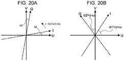
- FIGS. 20A and 20B The coordinate conversion using the orthogonality ⁇ and the phase correction value ⁇ is illustrated in FIGS. 20A and 20B.
- FIG. 20A illustrates a case where the orthogonality ⁇ between IQ axes and the UV axes is changed. In the case where 45° > ⁇ > 0°, the I-axis exists above the U-axis in the first quadrant and the Q-axis exists to the right of the V-axis.
- FIG. 20B illustrates a state in which the state shown in FIG. 20A is rotated by phase correction value ⁇ .
- the measurement angle error corrector 39 corrects the measurement angle error signals by using the correction parameters ⁇ , ⁇ , Ku, and Kv. For the purpose of illustrating the operation of the measurement angle error corrector 39, the following variables are defined.
- Xm The measurement angle error signal X corrected by the measurement angle error corrector 39.
- Ym The measurement angle error signal Y corrected by the measurement angle error corrector 39.
- the measurement angle error corrector 39 corrects the measurement angle error signals expressed by the following equation.
- Xm Ym cos ⁇ ⁇ ⁇ / Ku ⁇ sin ⁇ ⁇ ⁇ / Ku sin ⁇ + ⁇ / Kv cos ⁇ + ⁇ / Kv X Y
- the tracking controller 33A calculates a command value obtained by adding (i) the change caused by the orbit prediction value and (ii) the measurement angle error signals Xm and Ym corrected by the measurement angle error corrector 39 to (iii) the orientation direction actual measurement value.
- the correction value calculator 32A calculates Xfj and Yfj using Equation (41) and determines the correction parameters ( ⁇ , ⁇ , Ku, and Kv, Du, and Dv) such that the error function E defined by Equation (29) is minimized. Since there are six correction parameters, the number N of the error measurement data 55 is greater than or equal to four pieces. The greater N is, the more accurate calculation of the correction parameters becomes.
- Equation (30) ⁇ Xj 2 + Yj 2 ⁇ 2 ⁇ Ku ⁇ cos ⁇ 1 2 ⁇ ⁇ ⁇ Du ⁇ Uj ⁇ Xj ⁇ cos ⁇ + ⁇ ⁇ Yj ⁇ sin ⁇ + ⁇ ⁇ 2 ⁇ Kv ⁇ cos ⁇ 1 2 ⁇ ⁇ ⁇ Dv ⁇ Vj ⁇ Xj ⁇ sin ⁇ ⁇ ⁇ + Yj ⁇ cos ⁇ + ⁇ + 1 + sin 2 ⁇ ⁇ sin 2 ⁇ ⁇ Ku 2 ⁇ ⁇ Du ⁇ Uj 2 + 1 ⁇ sin 2 ⁇ ⁇ sin 2 ⁇ ⁇ sin 2 ⁇ ⁇ Kv 2 ⁇ ⁇ Dv ⁇ Vj 2 ⁇ 2 ⁇ sin 2 ⁇ ⁇ Ku ⁇ Kv ⁇ ⁇ Du ⁇ Uj ⁇ Dv ⁇ Vj ) ⁇ cos ⁇ 2 2 ⁇
- Ku and Kv are replaced as follows.
- Ku Ku / cos 2 ⁇
- Kv Kv / cos 2 ⁇
- Equation (44) is substituted with Equation (45) and Equation (46) as follows. Equation (44) may be used without substituting with Equation (45) and Equation (46).
- E ⁇ Xj 2 + Yj 2 ⁇ 2 ⁇ Ku ⁇ ⁇ Du ⁇ Uj ⁇ Xj ⁇ cos ⁇ + ⁇ ⁇ Yj ⁇ sin ⁇ + ⁇ ⁇ 2 ⁇ Kv ⁇ ⁇ Dv ⁇ Vj ⁇ Xj ⁇ sin ⁇ ⁇ ⁇ + Yj ⁇ cos ⁇ ⁇ ⁇ + 1 + sin 2 ⁇ ⁇ sin 2 ⁇ ⁇ Ku 2 ⁇ ⁇ Du ⁇ Uj 2 + 1 ⁇ sin 2 ⁇ ⁇ sin 2 ⁇ ⁇ Kv 2 ⁇ ⁇ Dv ⁇ Vj 2 ⁇ 2 ⁇ sin 2 ⁇ ⁇ Ku ⁇ Kv ⁇ ⁇ Du ⁇ Uj ⁇ Dv ⁇ Vj
- Equation (44A) As an equation without ⁇ , the following additional variables are defined.
- r 0 ⁇ x 0 2 + y 0 2 .
- ⁇ sin ⁇ 1 y 0 / r 0 .
- ws 0 ⁇ uj ⁇ vj ⁇ u 0 ⁇ v 0 / N .
- Equation (44A) becomes as follows.
- E N ⁇ xs 0 + ys 0 ⁇ 2 N ⁇ Ku ⁇ Du ⁇ u0 ⁇ r 0 ⁇ cos ⁇ + ⁇ + ⁇ + d 0 ⁇ cos ⁇ + ⁇ ⁇ e 0 ⁇ sin ⁇ + ⁇ ⁇ 2 N ⁇ Kv ⁇ Dv ⁇ v0 ⁇ r 0 ⁇ sin ⁇ + ⁇ ⁇ ⁇ + f 0 ⁇ sin ⁇ ⁇ ⁇ + g 0 ⁇ cos ⁇ ⁇ ⁇ + N ⁇ Ku 2 ⁇ Du ⁇ u0 2 ⁇ us 0 ⁇ 1 + sin 2 ⁇ ⁇ sin 2 ⁇ + N ⁇ Kv 2 ⁇ Dv ⁇ v0 2 ⁇ vs 0 ⁇ 1 + sin 2 ⁇ ⁇ sin 2 ⁇ ⁇ 2 ⁇ N ⁇ Ku ⁇ Kv 2 ⁇ Dv ⁇ v0 2 ⁇ vs
- ⁇ E/ ⁇ 0.
- approximate values are calculated by assigning initial values to ⁇ , ⁇ , Ku, Kv, Du, and Dv and by correcting the parameters by way of repeated calculation.
- X1j Xfj obtained before this time calculation.
- Y1j Yfj obtained before this time calculation.
- ⁇ xxj Error of X1j remained before this time calculation.
- ⁇ xxj Xj - X1j.
- ⁇ yyj Error of X1j remained before this time calculation.
- ⁇ yyj Yj - Y1j. ( ⁇ , ⁇ , ⁇ Ku, ⁇ Kv, ⁇ Du, ⁇ Dv): The change in correction parameters to be calculated this time.
- ⁇ xj Change of Xfj caused by the change of the correction parameters.
- ⁇ yj Change of Yfj caused by the change of the correction parameters.
- ⁇ G Error function for defining the change in the correction parameters.
- ⁇ G ⁇ ⁇ xxj ⁇ ⁇ xj 2 + ⁇ yyj ⁇ ⁇ yj 2
- Equation (48) By substituting the left side of Equation (48) with Equation (49) and Equation (50), the following is obtained.
- Equation (51) to Equation (56) Six linear equations are obtained in Equation (51) to Equation (56) with respect to six unknown variables ( ⁇ , ⁇ , ⁇ Ku, ⁇ Kv, ⁇ Du, ⁇ Dv).
- Equation (51) to Equation 56 Six linear equations are obtained in Equation (51) to Equation 56), ( ⁇ , ⁇ , ⁇ Ku, ⁇ Kv, ⁇ Du, ⁇ Dv) can be calculated.
- Equation (45) and Equation (46) In a case where Ku and Kv are converted in Equation (45) and Equation (46), Ku and Kv are calculated by inversely applying Equation (45) and Equation (46).
- the initial values of the correction parameters may be predetermined or may be calculated as follows based on the correction parameters ( ⁇ 0, K0, Du0, and Dv0) calculated by the method in Embodiment 1.
- ( ⁇ , ⁇ , Ku, Kv, Du, Dv) (0, ⁇ 0, K0, K0, Du0, Dv0)
- Equation (59) is converted to an equation without ⁇ as follows.
- E N ⁇ xs 0 + ys 0 ⁇ 2 N ⁇ Ku ⁇ Du ⁇ u 0 ⁇ r 0 ⁇ cos ⁇ + ⁇ + d 0 ⁇ cos ⁇ ⁇ e 0 ⁇ sin ⁇ ⁇ 2 N ⁇ Kv ⁇ Dv ⁇ v 0 ⁇ r 0 ⁇ sin ⁇ + ⁇ + f 0 ⁇ sin ⁇ + g 0 ⁇ cos ⁇ + N ⁇ Ku 2 ⁇ Du ⁇ u 0 2 + us 0 + Kv 2 ⁇ Dv ⁇ v 0 2 + vs 0
- m 0 e 0 2 ⁇ g 0 2 / vs 0 + 2 ⁇ d 0 ⁇ f 0 / us 0
- n 0 d 0 2 ⁇ f 0 2 / us 0 ⁇ 2 ⁇ e 0 ⁇ g 0 / vs 0
- E ⁇ Xj 2 + Yj 2 ⁇ 2 ⁇ K ⁇ ⁇ Du ⁇ Uj ⁇ Xj ⁇ cos ⁇ + ⁇ ⁇ Yj ⁇ sin ⁇ + ⁇ ⁇ 2 ⁇ K ⁇ ⁇ Dv ⁇ Vj ⁇ Xj ⁇ sin ⁇ ⁇ ⁇ + Yj ⁇ cos ⁇ ⁇ ⁇ + K 2 ⁇ 1 + sin 2 ⁇ ⁇ sin 2 ⁇ ⁇ ⁇ Du ⁇ Uj 2 + 1 ⁇ sin 2 ⁇ ⁇ sin 2 ⁇ ⁇ ⁇ Dv ⁇ Vj 2 ⁇ ⁇ 2 ⁇ sin 2 ⁇ ⁇ ⁇ Du ⁇ Uj ⁇ Dv ⁇ Uj ⁇ Dv ⁇ Uj
- Equation (62) is converted to an equation without ⁇ as follows.
- E N ⁇ xs 0 + ys 0 ⁇ 2 N ⁇ Ku ⁇ Du ⁇ u 0 ⁇ r 0 ⁇ cos ⁇ + ⁇ + ⁇ + d 0 ⁇ cos ⁇ + ⁇ ⁇ e 0 ⁇ sin ⁇ + ⁇ ⁇ 2 N ⁇ K ⁇ Dv ⁇ v 0 ⁇ r 0 ⁇ sin ⁇ + ⁇ ⁇ ⁇ + f 0 ⁇ sin ⁇ ⁇ ⁇ + g 0 ⁇ cos ⁇ ⁇ ⁇ + N ⁇ K 2 ⁇ 1 + sin 2 ⁇ ⁇ sin 2 ⁇ ⁇ Du ⁇ u 0 2 + us 0 + 1 ⁇ sin 2 ⁇ ⁇ sin 2 ⁇ ⁇ Dv ⁇ v 0 2 + vs 0 ⁇ 2 ⁇ sin 2 ⁇ ⁇ Du ⁇ u 0 + ws
- Equation (62A) is somewhat simpler that Equation (44B), Equation (62A) cannot be solved analytically. Similar to the case where ⁇ ⁇ 0 and Ku ⁇ Kv, it is necessary to solve by repeated calculation.
- the error function E2 represented by Ufj and Vfj obtained by correcting Xj and Yj may be set to be minimized.
- Equation (65A) ⁇ Xj ⁇ Uj / N Equation (65A) becomes as follows.
- E 2 N ⁇ Ku 2 ⁇ Du ⁇ u 0 2 + us 0 + N ⁇ Kv 2 ⁇ Dv ⁇ v 0 2 + vs 0 ⁇ 2 N ⁇ Ku ⁇ Du ⁇ u 0 ⁇ r 0 ⁇ cos ⁇ + ⁇ ⁇ ⁇ + d 0 ⁇ cos ⁇ ⁇ ⁇ ⁇ e 0 ⁇ sin ⁇ ⁇ ⁇ ⁇ 2 N ⁇ Kv ⁇ Dv ⁇ v 0 ⁇ r 0 ⁇ sin ⁇ + ⁇ + ⁇ + f 0 ⁇ sin ⁇ + ⁇ + N ⁇ 1 + sin 2 ⁇ ⁇ sin 2 ⁇ ⁇ xs 0 + N ⁇ 1 + sin 2 ⁇ ⁇ sin 2 ⁇ ⁇ xs 0 + N ⁇ 1 + sin 2 ⁇ ⁇ sin 2 ⁇ ⁇ x
- the orthogonality ⁇ , the phase correction value ⁇ , the AZ sensitivity coefficient Ku, and the EL sensitivity coefficient Kv may be calculated by minimizing the following error function E3.
- E 3 ⁇ Ufj ⁇ Uj 2 + Vfj ⁇ Vj 2
- the error function E3 is the sum of squares of post-correction residuals for N pieces of the error measurement data 55.
- the post-correction residuals are the respective differences between (i) the arrival direction errors (Du - Ufj, Dv - Vfj) corrected by correction parameters including the phase correction value y and (ii) the actual measurement value errors ((Du - Uj, Dv - Vj).
- a portion of the correction parameters among the orthogonality ⁇ , the phase correction value ⁇ , the AZ sensitivity coefficient Ku, and the EL sensitivity coefficient Kv may be used to correct the actual measurement values errors. Either the actual measurement value error or the arrival direction error is corrected by each of the correction parameters.
- correction parameters that minimizes the sum of squares of post-correction residuals for N pieces of the measurement error data can be obtained.
- the post-correction residuals are differences between a post-correction actual measurement value and a post-correction arrival direction error.
- the post-correction actual measurement value and the post-correction arrival direction error are the actual measurement value and the arrival direction error obtained after correcting based on each of the correction parameters.
- the correction parameters calculated by the correction value calculator 32A are stored in the data storage 34A.
- the values to be stored are the calculated values without further processing.
- FIG. 21 is a flowchart illustrating operation of the antenna control device according to Embodiment 2. The points that differ from those in FIG. 7 of Embodiment 1 are described.
- the correction value calculator 32A calculated the phase correction value ⁇ , the orthogonality ⁇ , the AZ sensitivity coefficient Ku, and the EL sensitivity coefficient Kv and stores this calculated data into the data storage 34A.
- the ⁇ , ⁇ , Ku, and Kv that had been calculated are stored in the data storage 34A. Since the coordinate converter 24 of the tracking receiver 8 cannot perform correction taking the orthogonality ⁇ into account and correction using sensitivity coefficients Ku and Kv that are different for the azimuth angle direction and the elevation angle direction, the data cannot be stored in the data storage 23 of the tracking receiver 8.
- the measurement angle error corrector 39 calculates the measurement angle error signals X and Y while taking into account the phase correction value ⁇ , the orthogonality ⁇ , the AZ sensitivity coefficient Ku, and the EL sensitivity coefficient Kv and outputs the measurement angle error signals Xm and Ym.
- the tracking controller 33A calculates the command value by adding the measurement angle error signals Xm and Ym to the orbit prediction value and outputs the command value to the antenna drive controller 27.
- the oscillation cause determiner 37A activates multiple times the error measurement data generator 31 and the correction value calculator 32A to calculate multiple sets of the phase correction value ⁇ , the AZ sensitivity coefficient Ku, and the EL sensitivity coefficient Kv.
- a check is performed as to whether or not oscillation is caused by phase shift.
- An example of the condition to determine that oscillation is caused by phase shift is that the values obtained by subtracting (i) y that is used by the measurement angle error corrector 39 from (ii) the calculated phase correction values ⁇ , are within a range not including zero degrees and having a predetermined width.
- step S14A the correction value updater 38A stores the newly calculated phase correction value y into the data storage 34. Since the measurement angle error signal that is outputted by the tracking receiver 8A in Embodiment 2 is not corrected by the phase correction value ⁇ , it is sufficient that the phase correction value y calculated by the correction value calculator 32A is stored without further processing.
- a check is performed as to whether or not oscillation is caused by sensitivity shift.
- Examples of the condition to determine that oscillation is caused by sensitivity shift are that the values obtained by dividing (i) the calculated AZ sensitivity coefficients Ku by (ii) Ku that is used by the measurement angle error corrector 39, are within a range not including 1 and having a predetermined width, or, that the values obtained by dividing (i) the calculated EL sensitivity coefficients Kv by (ii) Kv that is used by the measurement angle error corrector 39, are within a range not including 1 and having a predetermined width.
- the correction value updater 38A stores the newly calculated AZ sensitivity coefficient Ku and the EL sensitivity coefficient Kv into the data storage 34.
- the correction value calculator 32A calculates correction parameters such as the orthogonality ⁇ and sensitivity coefficients that are different for the azimuth angle direction and the elevation angle direction. Three examples are used to describe the correction parameters that are calculated by the correction value calculator 32A.
- the post-correction measurement angle error vector Vaj that is obtained by correcting the measurement angle error vector Vsj with the correction parameters ( ⁇ , ⁇ , Ku, Kv, Du, Dv) is illustrated in FIG. 22 .
- This Vaj is closer to the Vsj than the Vaj illustrated in FIG. 10 .
- the post-correction measurement angle error vector Vaj that is obtained by correcting the measurement angle error vector Vsj with the correction parameters ( ⁇ , ⁇ , Ku, Kv, Du, Dv) is illustrated in FIG. 23 .
- This Vaj is closer to the Vsj than the Vaj illustrated in FIG. 13 .
- FIGS. 24 to 26 The third example is illustrated in FIGS. 24 to 26 .
- the simulation conditions are set as indicated below.
- FIGS. 24 to 26 are expressed similarly to FIG. 8 to FIG. 10 .
- Orthogonality ⁇ -10°
- Kv 1 U-direction prediction value error
- Du 0.05°
- V-direction prediction value error Dv 0.03°
- FIG. 27 is a diagram illustrating a trajectory of the measurement angle error signal corrected by the phase correction value and the sensitivity coefficients calculated by the antenna control device according to Embodiment 1, as a comparison example. Since the orthogonality is not taken into account, the Vaj and the Vsj are slightly more apart from each other than those in FIG. 26 .
- Embodiment 2 since the orthogonality, the AZ sensitivity coefficient, and the EL sensitivity coefficient are taken into account, the correction parameters that correct the measurement angle error signal can be more accurately calculated than in the case of Embodiment 1.
- Embodiment 3 is a case where a calibration tower (collimation) is used to adjust the phase and sensitivity in advance. By doing so, when a moving object such as a rocket is tracked, tracking can be performed even when there is no orbit prediction value of the moving object or the accuracy of the orbit prediction value is low.
- a calibration tower collimation
- FIG. 28 is a diagram illustrating a configuration of an antenna system including an antenna control device according to Embodiment 3 of the present invention.
- FIG. 29 is a block diagram illustrating a configuration of an antenna control device according to Embodiment 3.
- An antenna system 100B includes a calibration tower 71.
- the calibration tower 71 emits a radio wave 11B of a predetermined frequency.
- the calibration tower 71 is installed at a position where the antenna 1 can receive the radio wave 11B emitted by the calibration tower 71.
- the calibration tower 71 is a test radio wave source that is installed on the ground at a predetermined position with respect to the antenna 1 and emits radio waves.
- the calibration tower 71 is a temporary communication counterpart during program tracking in order to acquire error measurement data for calculating correction parameters.
- An orbit prediction value of a moving object 10B does not exist. Therefore, the antenna control device 9B does not include an orbit prediction value data generator 26.
- a program controller 28B and a correction value calculator 32B are modified.
- a data storage 34B includes a change scenario 54B.
- the change scenario 54B is a scenario for changing the orientation direction of the antenna 1 in a way to be different from that in Embodiment 1.
- the program controller 28B defining the direction toward the calibration tower 71 as a reference direction, makes the orientation direction of the antenna 1 to change in a range that is within a predetermined maximum angle difference.
- FIG. 30 is a diagram illustrating an example of a trajectory in which the orientation direction is changed during program tracking by the antenna control device according to Embodiment 3.
- the orientation direction is stationary for at least a predetermined time.
- the offset angle ⁇ is determined such that the offset angle ⁇ exists in a linear region in which sensitivity coefficients are linear.
- the linear region is a region in which the
- the orientation direction of the antenna 1 changes in a state in which the elevation angle of the antenna 1 is close to zero. Therefore, the U-direction offset angle ⁇ , as it is, may be set as the change in the command value of the azimuth angle.
- the correction value calculator 32B calculates the phase correction value ⁇ , the AZ sensitivity coefficient Ku, and the EL sensitivity coefficient Kv, and the orthogonality ⁇ as follows.
- the relationship between the measurement angle error signals (X1, Y1) and (X2, Y2) with respect to G 1 and G 2 on the U-axis is illustrated in FIG. 31 .
- the relationship between the measurement angle error signals (X3, Y3) and (X4, Y4) with respect to G 3 and G 4 on the V-axis is illustrated in FIG. 32 .
- the U-axis and the V-axis are direction respectively are a first direction and a second direction orthogonal on the celestial sphere with the reference celestial sphere point G 0 being the reference.
- the orientation direction is stationary for a predetermined time at two celestial sphere points G 1 and G 2 on the U-axis being the first direction.
- the orientation direction is stationary for a predetermined time at two celestial sphere points G 3 and G 4 on the V-axis being the second direction.
- the correction value calculator 32B calculates at least the phase correction value ⁇ by using the equation for the error measurement data measured at the celestial sphere points G 1 and G 2 and the equation for the error measurement data measured at the celestial sphere points G 3 and G 4 .
- a time sequence example for driving automatically the antenna is illustrated in FIG. 33 .
- the antenna drive controller 27 is a servo-type that does not overshoot
- data acquisition is easy.
- the time during which the antenna 1 is oriented toward a single celestial sphere point is 7 seconds
- the data acquisition time is 3 seconds
- the data sampling time is 0.1 seconds.
- the time period during which data is acquired is 3 seconds anywhere from start to finish of the 7-second time period during which the antenna 1 is oriented toward a single celestial sphere point.
- the correction parameters ( ⁇ , ⁇ , Ku, Kv, Du, Dv) are calculated using the method indicated from Equation (71) to Equation (76) with respect to the value obtained by averaging the data acquired in the 3-second data acquisition time period.
- FIG. 34 illustrates the simulation results of measurement angle error signals X and Y.
- the measurement angle error signal X is represented by a bold solid line and the measurement angle error signal Y is represented by a solid line.
- the results of calculation by the correction value calculator 32B are as indicated below. Since no noise exists, values equal to the set conditions can be correctly calculated. The same results can be obtained by the correction value calculator 32A of Embodiment 2.
- the correction value calculator 32A uses all data during the time period including time when the orientation direction of the antenna is changing.
- the initial values of the correction value calculator 32A are the correction parameters calculated by the correction value calculator 32B.
- Orthogonality ⁇ -5.00°
- Phase correction value ⁇ 43.00°
- AZ sensitivity coefficient Ku 1.200
- Kv 0.850
- Du 0.05000°
- V-direction prediction value error Dv -0.03000°
- the simulation results of the measurement angle error signals in the case where noise superimposing on the measurement angle error signal is approximated using a Gauss random number and the effective value of that magnitude is set to be 0.01° rms are illustrated in FIG. 35 .
- the actual measurement value of the orientation direction of the antenna 1 is not superimposed with noise.
- the noise is approximately 18% of the offset angle.
- both the correction value calculator 32B and the correction value calculator 32A can calculate the phase correction value ⁇ and so on quite accurately.
- the noise is approximately 180% of the offset angle ⁇ .
- the noise is 10 times of that in FIG. 35 .
- Both the correction value calculator 32B and the correction value calculator 32A calculate correction parameters that do not cause the antenna servo system to oscillate, and thus it can be said that these methods are effective against noise.
- phase adjustment and sensitivity adjustment can be performed automatically by the calibration tower (collimation). Erroneous operation by human can be prevented and work efficiency can be enhanced.
- the correction parameters calculated at 4 points existing in the linear region can be used in a non-linear region effectively.
- FIG. 37 to FIG. 42 are used to describe this.
- FIG. 37 is a diagram illustrating measurement angle error signals that are not corrected by correction parameters such as the phase correction value in the case where the azimuth angle is changed.
- FIG. 38 is a diagram illustrating measurement angle error signals that are not corrected in the case where the elevation is changed.
- FIG. 39 is a diagram illustrating measurement angle error signals at 4 points in a linear region used for correction.
- the measurement angle error signals at 4 points can be obtained as illustrated in FIG. 40 .
- the measurement angle error signal X exists on the U-axis and the measurement angle error signal Y exists on the V-axis. It can be understood that the corrections are performed properly.
- FIG. 41 illustrates the corrected measurement angle error signals in the case where the azimuth angle is changed.
- FIG. 42 illustrates the corrected measurement angle error signals in the case where the elevation angle is changed. It can be understood that the corrections are performed almost properly even in the non-linear region.
- the simulation results illustrated in FIG. 41 and FIG. 42 show that the correction could be made even in the non-linear region by using the phase, orthogonality, and the sensitivity coefficients calculated using data at the 4 points, and that data at 4 points are sufficient for automatic adjustment using a calibration tower (collimation).
- the correction value calculator 32C in such a modified example calculates, for example, as follows.
- Celestial sphere points may be set for generating the error measurement data 55 at more than 3 points on the U-axis. ⁇ 1 and other parameters may be determined such that the sum of squares of the post-correction residuals is minimized similar to that in Embodiment 1. Celestial sphere points may be set for generating the error measurement data 55 at more than 3 points on the V-axis. ⁇ 2 and other parameters may be determined such that the sum of squares of the post-correction residuals is minimized similar to that in Embodiment 1. Celestial sphere points may be set for generating the error measurement data 55 at positions not on the U-axis or the V-axis. ⁇ , ⁇ , and other parameters may be calculated by taking into account at the same time all celestial sphere points for generating the error measurement data 55 similar to that in Embodiment 1.
- Embodiment 4 is a case where the signal intensity of the difference signal is received by an antenna control device and the offset angle ⁇ is changed in accordance with the signal intensity of the difference signal.
- this Embodiment is a modification of Embodiment 2, this can be similarly applied to Embodiment 1 as well.
- FIG. 43 is a diagram illustrating a configuration of an antenna system including an antenna control device according to Embodiment 4 of the present invention.
- a tracking receiver 8C also outputs the signal intensity of the difference signal (difference signal level R).
- FIG. 44 is a block diagram illustrating a configuration of the antenna control device according to Embodiment 4. The points that differ from those in FIG. 19 of Embodiment 2 are described.
- An antenna control device 9C that is included in an antenna system 100C includes an offset angle calculator 40.
- the offset angle calculator 40 changes the offset angle ⁇ in accordance with the difference signal level R. In a case where the difference signal level R is low, the offset angle ⁇ is increased such that a signal intensity is greater than or equal to the lower limit value.
- the data storage 34C is also modified.
- the data storage 34C is modified to include a standard offset angle 57 and an offset angle 58.
- a change scenario 54E is a scenario in which the offset angle 58 is used to change the command value of the orientation direction.
- a program controller 28C uses a changeable offset angle ⁇ to perform program control.
- the standard offset angle 57 is an angle used as offset angle ⁇ in a case where the difference signal level R is sufficiently high.
- the offset angle 58 is an offset angle that is calculated by the offset angle calculator 40 in accordance with the difference signal level R.
- ⁇ 0 Standard offset angle.
- ⁇ max Upper limit value of offset angle ⁇ . For example, approximately 60% of the half width of the antenna 1 is set.
- R Difference signal level.
- Rmin Lower limit value with respect to the difference signal level R.
- S Reception level.
- Smin Lower limit value with respect to the reception level S.
- fr ( ⁇ , R) Function for predicting the difference signal level R with respect to the offset angle ⁇ . R increases as ⁇ increases.
- fs ( ⁇ , S) Function for predicting the reception level S with respect to the offset angle ⁇ . S decreases as ⁇ increases.
- fr ( ⁇ , R) and fs ( ⁇ , S) are functions derived by approximating the antenna pattern by a gauss function, for example.
- the standard offset angle ⁇ 0 is determined such that calculation accuracy of the correction parameters calculated using the error measurement data of N-pieces is greater than or equal to the required accuracy in a case where the difference signal level R is the lower limit value Rmin.
- the offset angle calculator 40 calculates the offset angle in accordance with the difference signal level R and the reception level S as follows.
- the minimum ⁇ in the range may be determined. If the difference signal level R and the reception signal S are divided into multiple ranges, a ⁇ determined to satisfy the condition of each range in the multiple ranges may be used.
- FIG. 45 is a flowchart illustrating operation of the antenna control device according to Embodiment 4. The points that differ from those in FIG. 7 of Embodiment 1 are described.
- Step S21 is added immediately before step S06C.
- the offset angle calculator 40 determines the offset angle ⁇ based on the reception level S and the difference signal level R.
- the orientation direction of the antenna is changed in accordance with a change scenario 54C in which the offset angle ⁇ is used.
- correction parameters such as the phase correction value ⁇ can be calculated in a state in which the signal intensity of the difference signal is higher than that in Embodiment 2 and without causing the reception level S to be reduced more than necessary.
- the determining of the offset angle ⁇ based on the difference signal level R is equivalent to determining the offset angle ⁇ in accordance with the signal-to-noise ratio (SN ratio) provided that the level of noise is constant.
- the offset angle ⁇ may be determined based on the SN ratio of the difference signal instead of the difference level R.
- the offset angle calculator is a change reference angle determiner that determines an offset angle ⁇ such that the signal intensity of the difference signal or the signal-to-noise ratio is greater than or equal to a lower limit value.
- Embodiment 5 is a case in which a SN ratio of a difference signal is received by the antenna control device and a length of a period for performing program tracking is changed in accordance with the SN ratio of the difference signal.
- FIG. 46 is a diagram illustrating a configuration of an antenna system including an antenna control device according to Embodiment 5 of the present invention.
- a tracking receiver 8D outputs the SN ratio Z of the difference signal to an antenna control device 9D.
- FIG. 47 is a block diagram illustrating a configuration of the antenna control device according to Embodiment 5. The points that different from those in FIG. 19 of Embodiment 2 are described.
- the antenna control device 9D included in the antenna system 100D includes a program operation period setter 41.
- the program operation period is a time period during which the command value of the orientation direction is changed in accordance with the change scenario.
- the program operation period setter 41 changes the length of the program operation period in accordance with the SN ratio of the difference signal.
- the program operation period setter 41 increases the length of the program operation period in a case where the SN ratio of the difference signal is less than or equal to a lower limit value.
- the program controller 28D uses a changeable program operation period to perform program control.
- the program operation period is set such that the calculation accuracy of the correction parameters calculated by the correction value calculator 32A is greater than or equal to a predetermined accuracy.
- Reason being, the values that minimize the average of signals containing error have improved SN ratio than that of the original signal.
- Z the SN ratio of an original signal
- Z the SN ratio of an average value of signals of ⁇ -pieces
- the value that minimizes the square error with respect to data of ⁇ -pieces of a single variable is the average value of data of ⁇ -pieces. It can be considered that the SN ratio of variable value that minimizes the square error of multiple variables also is Z ⁇ ⁇ ( ⁇ ).
- a data storage 34D is also modified.
- the data storage 34D includes a standard program operation period 59 and a program operation period 60.
- the change scenario 54D is a scenario that uses the program operation period 60 in changing the command value of the orientation direction.
- the standard program operation period 59 is a length of time (program operation period) during which program tracking is performed in accordance with the change scenario 54D in the case where the difference signal level R is sufficiently high.
- the program operation period 60 is a program operation period set by the program operation period setter 41.
- the error measurement data 53 is generated at a predetermined time interval during operation in accordance with the change scenario 54D.
- Ts The program operation period.
- Ts0 Standard program operation period.
- Tmax Upper limit value of the program operation period.
- Z SN ratio of the difference signal.
- Zmin Lower limit value with respect to the SN ratio of the difference signal.
- the number N of error measurement data for the standard program operation period Ts0 can be determined such that calculation accuracy of the correction parameters calculated based on the error measurement data of N-pieces is greater than or equal to the required accuracy in a case where the SN ratio Z of the difference signal is the lower limit value Zmin.
- the program operation period setter 41 sets the program operation period Ts in accordance with the SN ratio Z of the difference signal as follows.
- the program operation period Ts may be set for each range of the SN ratio of the difference signal.
- a Ts for each range may be determined (i) such that the calculation accuracy of the correction parameters is greater than or equal to the predetermined accuracy and (ii) to be monotonically non-decreasing with respect to increases in the SN ratio.
- FIG. 48 is a flowchart illustrating operation of the antenna control device according to Embodiment 5. The points that differ from those in FIG. 45 of Embodiment 4 are described.
- step S21D the program operation period setter 41 sets the program operation period Ts based on the SN ratio Z of the difference signal.
- step S06D the command value of the orientation direction of the antenna is changed in accordance with the change scenario in which program operation period Ts is used.
- correction parameters such as the phase correction value ⁇ can be calculated at calculation accuracy that is greater than or equal to the predetermined accuracy.
- the program operation period Ts may be determined.
- the program operation period setter is a data count number determiner that determines a program operation period to be monotonically non-decreasing with respect to decreases in signal intensity or a signal-to-noise ratio in a case where the signal intensity or the signal-to-noise ratio of the difference signal is below a threshold.
- Embodiment 6 is a case in which a difference signal level is received by antenna control device and an offset angle and a length of a period for performing program tracking is changed in accordance with the difference signal level.
- the calculation accuracy of the correction parameters calculated by the correction value calculator 32A in a case where either the offset angle or the length of the period is changed during which program tracking is performed cannot reach or exceed the predetermined accuracy, the predetermined accuracy can be reached or exceeded by changing both the offset angle and the length of time during which the program tracking is performed.
- FIG. 49 is a diagram illustrating a configuration of an antenna system including an antenna control device according to Embodiment 6 of the present invention.
- a tracking receiver 8C outputs a difference signal R to an antenna control device 9D.
- FIG. 50 is a block diagram illustrating a configuration of the antenna control device according to Embodiment 6. The points that differ from those in FIG. 44 of Embodiment 4 are described.
- the antenna control device 9E that is included in an antenna system 100E includes a program operation period setter 41E.
- the program operation period setter 41E changes the length of a program operation period in accordance with the difference signal level R. In a case where the difference signal R is less than or equal to a lower limit value, the program operation period setter 41E increases the length of the program operation period such that the difference signal level R is greater than or equal to the lower limit value.
- a data storage 34E also includes the standard program operation period 59 and the program operation period 60.
- the change scenario 54E is a scenario in which the offset angle 58 and the program operation period 60 are used to change the command value of the orientation direction.
- An offset angle calculator 40E is also modified.
- a program controller 28E uses a changeable offset angle ⁇ and a changeable program operation period Ts to perform program control.
- the number N of the error measurement data for a case in that the standard offset angle ⁇ 0 and the standard program operation period Ts0 is determined such that calculation accuracy of the correction parameters calculated based on the error measurement data of N-pieces is greater than or equal to the required accuracy in a case where the difference signal level R is the lower limit value Rmin.
- the offset angle ⁇ is changed in a case in which calculation accuracy of the correction parameters cannot reach or exceed the predetermined accuracy by lengthening the program operation period Ts. Since the lengthening of the program operation period Ts does not bring a reduction in the reception level S, it is preferable lengthening the program operation period Ts is applied preferentially in a case where not reducing the reception level S is given higher priority.
- the program operation period setter 41E sets the program operation period Ts in accordance with the difference signal R as follows.
- the offset angle calculator 40E operates similarly to the offset angle calculator 40.
- the offset angle calculator 40E operates similarly to the offset angle calculator 40.
- the program operation period setter 41E operates similarly to a case when the program operation period Ts is determined first.
- FIG. 51 is a flowchart illustrating operation of the antenna control device according to Embodiment 5. The points that differ from those in FIG. 48 of Embodiment 5 are described.
- step S21E the program operation period setter 41E sets the program operation period Ts based on the difference signal level R.
- the offset angle calculator 40E determines the offset angle ⁇ based on the reception level S and the difference signal level R.
- the difference signal level R is a value considering the program operation period Ts.
- step S06E the command value of the orientation direction of the antenna is changed in accordance with a change scenario in which the offset angle ⁇ and the program operation period Ts is used.
- the offset angle ⁇ and the program operation period Ts are determined in accordance with the difference signal level R without causing the reception level S to be reduced more than necessary, and thus the correction parameters such as the phase correction value ⁇ can be calculated with the SN ratio of the difference signal in a state that is better than that in Embodiment 2.
Landscapes
- Physics & Mathematics (AREA)
- Engineering & Computer Science (AREA)
- General Physics & Mathematics (AREA)
- Radar, Positioning & Navigation (AREA)
- Remote Sensing (AREA)
- Variable-Direction Aerials And Aerial Arrays (AREA)
Abstract
Description
- The present invention relates to a device for controlling an antenna device that is installed on the ground, receives radio waves from a moving object such as an artificial satellite and tracks the moving object.
- There is a control device that performs automatic tracking to orient an antenna toward a moving satellite by obtaining a deviation between a direction from an installation position of the antenna installed at a ground station to the moving satellite which goes around the Earth and a direction in which the main reflector of the antenna is oriented (referred to as the main beam axis), and controlling the main beam axis of the antenna such that this deviation approaches zero (see Patent Literature 1).
- The tracking device described in
Patent Literature 1 receives, by the antenna, radio waves (signals) transmitted from the moving satellite, and derives, based on the received signals, a sum signal and a difference signal. An auxiliary power supply system provided in a power supply circuit of the antenna derives the sum signal and the difference signal. Examples of a method for deriving the sum signal and the difference signal include a multi-horn scheme, a high-dimensional scheme, and a combination scheme. The sum signal is a signal that is a total of signals received at portions of the antenna and indicates a maximum value when the main beam axis of the antenna aligns with the direction to the moving satellite. The difference signal is a signal that is a difference in signals received at the portions of the antenna and indicates a minimum value when the main beam axis of the antenna aligns with the direction to the moving satellite. The absolute value for the magnitude of the difference signal denotes the magnitude of the deviation of the main beam axis. The phase difference between the sum signal and the difference signal denotes a direction of the deviation of the main beam axis on a celestial sphere. - Here, the sum signal and the difference signal have phases unmatched with each other. One of the reasons for causing this unmatched phase condition is a difference in line lengths between the sum signal and the difference signal in complicated circuits, which processes the sum signal and the difference signal, including a low-noise amplifier and a frequency converter. If the phase difference between the sum signal and the difference signal is not correct, the main beam axis cannot be oriented in a direction from which radio waves come and arrive from the moving satellite, because the main beam axis is controlled using a measurement angle error signal generated based on the phase difference. Therefore, before performing automatic tracking, the phase of the measurement angle error signal is adjusted such that the measurement angle error signal is oriented in the direction indicated by the deviation of the main beam axis on the celestial sphere.
- One of the methods for adjusting the phase of the measurement angle error signal is a method for phase adjustment by receiving radio waves emitted by the sun and then tracking the sun (see Patent Literature 2). Another method is, before starting automatic tracking, obtaining two vectors at each of two difference points in time, that is, (i) a first vector representing a difference between a direction of a command value of the main beam axis and an actual direction and (ii)a second vector representing a deviation of the main beam axis obtained based on the sum signal and the difference signal, and adjusting the phase of the measurement angle error signal to make the difference vector between two of the first vectors and the difference vector between two of the second vectors to be the same vector (see Patent Literature 3).
-
- Patent Literature 1: Unexamined Japanese Patent Application Kokai
Publication No.H11-38112 - Patent Literature 2: Japanese Patent No.
3678154 - Patent Literature 3: Japanese Patent No.
6004896 - Different frequencies are used for different satellites and phase shift changes depending on the frequency of the radio waves. In the method described in
Patent Literature 2, each time a different satellite is tracked, it is necessary tracking the sun to adjust the phase. Also, in a case where the antenna beam half width is small compared to the angular diameter of the sun, output of the measurement angle error signal either drops or stops completely. Consequently, the method for adjusting by tracking the sun cannot be used for the antenna with antenna beams having a narrow half width. -
Patent Literature 3 is a literature regarding a method where the phase is adjusted for tracking a satellite, without the use of the sun. The adjustment accuracy of the algorithm described inPatent Literature 3 in calculating the phase to be adjusted becomes worse in a case where the radio wave strength is weak, or, in other words, the signal-to-noise ratio is low. When tracking control is performed based on a measurement angle error signal with an inaccurately adjusted phase, the accuracy of tracking becomes worse, and in a worst case, tracking cannot be performed. An objective of the present invention is to be able to track a communication counterpart more accurately than conventional methods even in the case where the radio wave signal-to-noise ratio is low. - A control device according to the present invention includes:
- an antenna drive being inputted a command value of an orientation direction and to control an antenna driver for changing the orientation direction, the orientation direction being a direction in which an antenna for receiving radio waves from a communication counterpart to generate reception signals is oriented, such that a difference between the command value and the orientation direction approaches zero,
- a program controller to generate the command value being changed in accordance with a predetermined change scenario, and to output the generated command value to the antenna drive controller;
- an error measurement data generator to generate error measurement data including (i) an arrival direction error obtained from a sum signal and a difference signal of the reception signals, the arrival direction error representing a difference between the orientation direction and an arrival direction being a direction from which the radio waves come and arrive and (ii) an orientation direction actual measurement value being an actual measurement value of the orientation direction when the reception signals used to obtain the arrival direction error are received;
- a correction value calculator to calculate, based on at least three pieces of the error measurement data being obtained at conditions in which the program controller outputs the command values being different each other, a phase correction value being an angle by which the arrival direction error is rotated; and
- a tracking controller to output, to the antenna drive controller, as the command value, a value obtained by adding (i) the arrival direction error corrected based on the phase correction value to (ii) the orientation direction actual measurement value.
- According to the present invention, a communication counterpart can be more accurately tracked than with conventional methods even in the case where the radio wave signal-to-noise ratio is low.
-
- FIG. 1
- is a diagram illustrating a configuration of an antenna system including an antenna control device according to
Embodiment 1 of the present invention; - FIG. 2
- is a diagram illustrating an example of changes, with respect to an offset angle, of a sum signal and a difference signal that are generated by an antenna and inputted to a tracking receiver;
- FIG. 3
- is a block diagram illustrating a configuration of the tracking receiver;
- FIG. 4
- is a block diagram illustrating a configuration of the antenna control device according to
Embodiment 1; - FIG. 5
- is a diagram illustrating an example of a trajectory in which an orientation direction is changed when program tracking is performed by the antenna control device according to
Embodiment 1; - FIGS. 6A, 6B and 6C
- are diagrams illustrating a process for correcting a measurement angle error vector based on a phase correction value and a sensitivity coefficient calculated by the antenna control device according to
Embodiment 1; - FIG. 7
- is a flowchart illustrating a procedure for tracking a moving object by the antenna control device according to
Embodiment 1; - FIG. 8
- is a diagram illustrating an example of a trajectory of a measurement angle error signal and actual measurement value of an orientation direction measured when the orientation direction is changed in order to calculate a correction parameter by the antenna control device according to
Embodiment 1; - FIGS. 9A, 9B, 9C, 9D and 9E
- are diagrams illustrating temporal changes of measurement data in the case of
FIG. 8 ; - FIG. 10
- is a diagram illustrating a trajectory of the measurement angle error signal and the actual measurement value of the orientation direction, in the case of
FIG. 8 , corrected by the phase correction value and the sensitivity coefficient; - FIG. 11
- is a diagram illustrating another example of a trajectory of the measurement angle error signal and the actual value of the orientation direction measured when the orientation direction is changed in order to calculate the correction parameter by the antenna control device according to
Embodiment 1; - FIGS. 12A, 12B, 12C, 12D and 12E
- are a diagrams illustrating temporal changes of measurement data in the case of
FIG. 11 ; - FIG. 13
- is a illustrating a trajectory of the measurement angle error signal and the actual measurement value of the orientation direction, in the case of
FIG. 11 , corrected by the phase correction value and the sensitivity coefficient; - FIG. 14
- is a diagram illustrating temporal changes of actual measurement values of the azimuth angle and the elevation angle caused by phase shift between the measurement angle error signals during automatic tracking;
- FIGS. 15A and 15B
- are diagrams illustrating temporal changes of the phase correction value and the sensitivity coefficient for the case illustrated in
FIG. 14 ; - FIG. 16
- is a diagram illustrating temporal changes of the actual measurement values of the azimuth angle and the elevation angle caused by shift of the sensitivity coefficient of the measurement angle error signal during automatic tracking;
- FIGS. 17A and 17B
- are diagrams illustrating temporal changes of the phase correction value for the case illustrated in
FIG. 16 ; - FIG. 18
- is a diagram illustrating a configuration of an antenna system including an antenna control device according to
Embodiment 3 of the present invention; - FIG. 19
- is a block diagram illustrating a configuration of the antenna control device according to
Embodiment 2; - FIGS. 20A and 20B
- are diagrams illustrating relationships between drive axes of the antenna and detection axes of the tracking receiver;
- FIG. 21
- is a flowchart illustrating operation of the antenna control device according to
Embodiment 2; - FIG. 22
- is a diagram illustrating a trajectory of the measurement angle error signal and the actual measurement value of the orientation direction, in the case of
FIG. 8 , corrected by orthogonality, a phase correction value, an AZ sensitivity coefficient, and an EL sensitivity coefficient that are calculated by the antenna control device according toEmbodiment 2; - FIG. 23
- is a diagram illustrating a trajectory of the measurement angle error signal and the actual measurement value of the orientation direction, in the case of
FIG. 11 , corrected by the orthogonality, the phase correction value, the AZ sensitivity coefficient, and the EL sensitivity coefficient that are calculated by the antenna control device according toEmbodiment 2; - FIG. 24
- is a diagram illustrating an example of a trajectory of the measurement angle error signal and the actual measurement value of the orientation direction measured when the orientation direction is changed in order to calculate the correction parameter by the antenna control device according to
Embodiment 2; - FIGS. 25A, 25B, 25C, 25D and 25E
- are diagrams illustrating temporal changes of the measurement data in the case of
FIG. 24 ; - FIG. 26
- is a diagram illustrating a trajectory of the measurement angle error signal and the actual measurement value of the orientation direction corrected by the orthogonality, the phase correction value, the AZ sensitivity coefficient, and the EL sensitivity coefficient in the case of
FIG. 24 ; - FIG. 27
- is a diagram illustrating a trajectory of the measurement angle error signal and the actual measurement value of the orientation direction corrected by the phase correction value and the sensitivity coefficients that are calculated by the antenna control device according to
Embodiment 1, as a comparison example in the case ofFIG. 24 ; - FIG. 28
- is a diagram illustrating a configuration of the antenna system including the antenna control device according to
Embodiment 3 of the present invention; - FIG. 29
- is a block diagram of the antenna control device according to
Embodiment 3; - FIG. 30
- is a diagram illustrating an example of a trajectory in which the orientation direction is changed during program tracking by the antenna control device according to
Embodiment 3; - FIG. 31
- is a diagram illustrating a measurement angle error signal that is obtained in a case where the orientation direction is changed on the U-axis in order to calculate the correction parameter by the antenna control device according to
Embodiment 3; - FIG. 32
- is a diagram illustrating a measurement angle error signal that is obtained in a case where the orientation direction is changed on the V-axis in order to calculate the correction parameter by the antenna control device according to
Embodiment 3; - FIG. 33
- is a diagram illustrating a time sequence example in which the antenna is automatically driven by the antenna control device according to
Embodiment 3; - FIG. 34
- is a diagram illustrating measurement angle error signals generated by tracking receiver without superimposed noise in a case where the antenna is automatically driven as illustrated in
FIG. 33 ; - FIG. 35
- is a diagram illustrating an example of measurement angle error signals generated by tracking receiver with superimposed noise in the case where the antenna is automatically driven as illustrated in
FIG. 33 ; - FIG. 36
- is diagram illustrating another example of measurement angle error signals generated by tracking receiver with superimposed noise in the case where the antenna is automatically driven as illustrated in
FIG. 33 ; - FIG. 37
- is a diagram illustrating measurement angle error signals not being corrected and obtained in a case where the azimuth angle is changed by the antenna control device according to
Embodiment 3; - FIG. 38
- is a diagram illustrating measurement angle error signals not being corrected and obtained in a case where the elevation angle is changed by the antenna control device according to
Embodiment 3; - FIG. 39
- is a diagram illustrating four points of measurement angle error signals used for correction by the antenna control device according to
Embodiment 3; - FIG. 40
- is a diagram illustrating measurement angle error signals corrected at four points by the antenna control device according to
Embodiment 3; - FIG. 41
- is a diagram illustrating corrected measurement angle error signals obtained in a case where the azimuth angle is changed by the antenna control device according to
Embodiment 3; - FIG. 42
- is a diagram illustrating corrected measurement angle error signals obtained in a case where the elevation angle is changed by the antenna control device according to
Embodiment 3; - FIG. 43
- is a diagram illustrating a configuration of an antenna system including an antenna control device according to Embodiment 4 of the present invention;
- FIG. 44
- is a diagram illustrating a configuration of the antenna control device according to Embodiment 4;
- FIG. 45
- is a flowchart illustrating operation of the antenna control device according to Embodiment 4;
- FIG. 46
- is a diagram illustrating a configuration of an antenna system including an antenna control device according to
Embodiment 5 of the present invention; - FIG. 47
- is a block diagram illustrating a configuration of an antenna control device according to
Embodiment 5; - FIG. 48
- is a flowchart illustrating operation of the antenna control device according to
Embodiment 5; - FIG. 49
- is a diagram illustrating a configuration of an antenna system including an antenna control device according to
Embodiment 6 of the present invention; - FIG. 50
- is a block diagram illustrating a configuration of the antenna control device according to
Embodiment 6; and - FIG. 51
- is a flowchart illustrating operation of the antenna control device according to
Embodiment 6. - An antenna system including a control device according to
Embodiment 1 of the present invention is described with reference toFIG. 1 to FIG. 4 . Anantenna system 100, as illustrated inFIG. 1 , mainly includes anantenna 1, anantenna mount 2, anantenna driver 3, a power supply device 4, a sumsignal amplification converter 5, a differencesignal amplification converter 6, asignal receiver 7, a trackingreceiver 8, and anantenna control device 9. - The
antenna 1 receives aradio wave 11 from a movingobject 10 such as a satellite or a rocket. Theantenna mount 2 supports theantenna 1 to be able to change an orientation direction that is a direction in which theantenna 1 is oriented. Theantenna driver 3 drives theantenna mount 2 thereby changing the orientation direction of theantenna 1. The power supply device 4 supplies power to theantenna 1 after amplifying a transmission signal, and generates, based on reception signals received by theantenna 1, a sum signal (SUM) and a difference signal (ERROR) by using the auxiliary power supply system of the power supply device 4. The sumsignal amplification converter 5 amplifies the sum signal and converts the signal to an intermediate frequency. The differencesignal amplification converter 6 amplifies the difference signal and converts the signal to the intermediate frequency. Thesignal receiver 7 demodulates the sum signal and acquires data transmitted by the movingobject 10. The trackingreceiver 8 generates, from the sum signal and the difference signal, measurement angle error signals X and Y for driving theantenna mount 2. Theantenna control device 9 controls theantenna driver 3 such that theantenna 1 is oriented in the arrival direction. The arrival direction is a direction from which the radio wave transmitted by the movingobject 10 comes and arrives. - The orientation direction of the
antenna 1 is measured by anorientation direction measurer 12. The orientation direction of theantenna 1 can be changed by theantenna mount 2. The orientation direction is expressed by an azimuth angle and an elevation angle. Theorientation direction measurer 12 is inputted with signals outputted by angle detection encoders (an encoder for the azimuth angle and an encoder for the elevation angle) that are attached to theantenna 1. Theorientation direction measurer 12 measures the actual measurement value of the azimuth angle (referred to as the AZ actual angle) of the main beam axis of theantenna 1 based on the signal outputted by the encoder for the azimuth angle, and measures the actual measurement value of the elevation angle (referred to as the EL actual angle) of the main beam axis based on the signal outputted by the encoder for the elevation angle. Theorientation direction measurer 12 outputs the AZ actual angle and the EL actual angle to theantenna control device 9. The orientation direction is represented by a horizon coordinate system based on a combination of (i) an azimuth angle where north is zero degrees and clockwise angles from north are positive and (ii) an elevation angle where directing the horizon is zero degrees. - The
antenna mount 2 includes anelevation angle mount 13, anazimuth angle mount 14, and abase 15. Theelevation angle mount 13 supports theantenna 1. Theazimuth angle mount 14 supports the elevation angle mount 13 rotatably around an elevation angle axis (EL-axis) extending horizontally. Thebase 15 supports the azimuth angle mount 14 rotatably around an azimuth angle axis (AZ-axis) extending vertically. The azimuth angle may be referred to as an AZ-angle or AZ. The EL angle also may be referred to as an EL-angle or EL. Theantenna control device 9 can be applied also to an X/Y type of antenna mount. - The
antenna driver 3 includes anelevation angle driver 16 and anazimuth angle driver 17. Theelevation angle driver 16 changes the elevation angle of the elevation angle mount 13 relative to theazimuth angle mount 14. Theazimuth angle driver 17 changes the azimuth angle of the azimuth angle mount 14 relative to thebase 15. Theelevation angle driver 16 and theazimuth angle driver 17 each have a servo control system. - The power supply device 4 amplifies a transmission signal of a microwave frequency band to a predetermined power and supplies the amplified power to the
antenna 1. Furthermore, the power supply device 4 generates, based on the reception signals received by theantenna 1, a sum signal (SUM) and a difference signal (ERROR) by using the auxiliary power supply system of the power supply device 4. The sumsignal amplification converter 5 amplifies the sum signal and converts the frequency of the amplified sum signal to a lower frequency. The differencesignal amplification converter 6 amplifies the difference signal and converts the frequency of the amplified difference signal to the lower frequency. Thesignal receiver 7 processes the sum signal received from the sumsignal amplification converter 5 as a modulated communication signal and demodulates the processed signal. The sum signal and the difference signal are inputted to the trackingreceiver 8. -
FIG. 2 is a diagram illustrating an example of changes, with respect to an offset angle, of the sum signal and the difference signal that are generated by theantenna 1 and inputted to the trackingreceiver 8. InFIG. 2 , the sum signal is represented by a solid line and the difference signal is represented by a dashed line. The offset angle is an angle by which the orientation direction changes from a state of directing the movingobject 10. The offset angle is zero degrees when the orientation direction of theantenna 1 is oriented toward the movingobject 10. In a case where the offset angle is zero degrees, the signal intensity of the sum signal is at its highest, whereas the signal intensity of the difference signal is at its lowest. - The tracking
receiver 8 generates, based on the sum signal and the difference signal, measurement angle error signals X and Y for driving theantenna 1, and outputs the measurement angle error signals X and Y to theantenna control device 9. In a case where the phase difference between the sum signal and the difference signal is the same as the phase difference that is actually generated, the measurement angle error signal X corresponds to an azimuth angle error of the orientation direction and the measurement angle error signal Y corresponds to an elevation angle error of the orientation direction. - The
antenna control device 9 generates a drive signal for controlling the azimuth angle and the elevation angle of the main beam axis of theantenna 1 and outputs the drive signal to theantenna driver 3. Theantenna control device 9 controls the azimuth angle and the elevation angle of the main beam of theantenna 1 based on the measurement angle error signals. The controlling, based on measurement angle error signals, such that the measurement angle error signals approach zero, is referred to as automatic tracking. - A method in which the direction of the main beam of the
antenna 1 is controlled in accordance with a predetermined change scenario is referred to as program tracking. In program tracking, there is a case where control is performed based on an orbit prediction value, inputted from the external, of the movingobject 10 and the change scenario and a case where control is performed only by either the change scenario or the orbit prediction value. The orbit prediction value is data representing the position of the movingobject 10 per a predetermined width of time. The position of the movingobject 10 is represented by an azimuth angle and an elevation angle in the direction, on the celestial sphere, of the movingobject 10 as viewed from a predetermined observation point. The orbit prediction values inputted from the external, for example, every second, are interpolated by interpolation calculation to obtain values at a finer time width of 10 msec, for example. Theantenna control device 9 uses the interpolated orbit prediction values. - The configuration of the tracking
receiver 8 is described with reference toFIG. 3. FIG. 3 is a block diagram illustrating the configuration of the tracking receiver. The trackingreceiver 8, as illustrated inFIG. 3 , includes a sumsignal AGC circuit 18, a differencesignal AGC circuit 19, a 90degree phase shifter 20, an I-signal detector 21, a Q-signal detector 22, adata storage 23, a coordinateconverter 24, and aninterface 25. AGC is an abbreviation of automatic gain control, that is, automatic amplification ratio control. - The sum
signal AGC circuit 18 is inputted with a sum signal outputted by theantenna 1, the sumsignal AGC circuit 18 amplifies the inputted sum signal. The amplification ratio of the sumsignal AGC circuit 18 changes in accordance with the amplitude of the sum signal. The sumsignal AGC circuit 18 outputs the amplified sum signal to the 90degree phase shifter 20 and the I-signal detector 21. The sumsignal AGC circuit 18 outputs, to the differencesignal AGC circuit 19, an amplification voltage. The amplification voltage increases in proportion to the increase in the amplification ratio. - The difference
signal AGC circuit 19 is inputted with the difference signal outputted by theantenna 1 and the amplification voltage outputted by the sumsignal AGC circuit 18. The differencesignal AGC circuit 19 changes the amplification ratio in accordance with the value of the amplification voltage inputted from the sumsignal AGC circuit 18 and amplifies the inputted difference signal. That is, the differencesignal AGC circuit 19 amplifies the inputted difference signal by the amplification ratio that is proportional to the amplification ratio of the sumsignal AGC circuit 18. Consequently, the amplified difference signal outputted from the differencesignal AGC circuit 19 is amplified by the amplification ratio that is proportional to the amplification ratio of the amplified sum signal outputted from the sumsignal AGC circuit 18. The differencesignal AGC circuit 19 outputs the amplified difference signal to the I-signal detector 21 and the Q-signal detector 22. - The 90
degree phase shifter 20 shifts (changes) the phase of the amplified sum signal outputted from the sumsignal AGC circuit 18 by 90 degrees. The 90degree phase shifter 20 outputs, to the Q-signal detector 22, the amplified sum signal with phase shifted by 90 degrees. The shifting of the phase by 90 degrees means that the phase is increased by 90 degrees. - The I-
signal detector 21 detects the difference signal that is outputted from the differencesignal AGC circuit 19 by the sum signal (sum signal without phase shifting) that is outputted from the sumsignal AGC circuit 18. In other words, the I-signal detector 21 outputs a product of the sum signal outputted from the sumsignal AGC circuit 18 and the difference signal outputted from the differencesignal AGC circuit 19. The I-signal detector 21 outputs the detected signal (hereinafter referred to as the "I-signal") to the coordinateconverter 24. The axis where the I-signal is detected is referred to as the I-axis. - The Q-
signal detector 22 detects the difference signal outputted from the differencesignal AGC circuit 19 by the sum signal outputted from the 90degree phase shifter 20. In other words, the Q-signal detector 22 outputs the product of the sum signal outputted from the 90degree phase shifter 20 and the difference signal outputted from the differencesignal AGC circuit 19. The Q-signal detector 22 outputs the detected signal (hereinafter referred to as the "Q-signal") to the coordinateconverter 24. The axis where the Q-signal is detected is referred to as the Q-axis. - The
phase correction value 51 and thesensitivity coefficient 52 used by the coordinateconverter 24 are stored in thedata storage 23. Thephase correction value 51 and thesensitivity coefficient 52 are calculated by theantenna control device 9. Thephase correction value 51 is a correction value by which the phase of the I-axis and the Q-axis are corrected. With thephase correction value 51, the I-axis where the measurement angle error signal X is detected aligns with a U-axis (described later) that corresponds to the azimuth angle of the orientation direction and the Q-axis where the measurement angle error signal Y is detected aligns with a V-axis (described later) that corresponds to the elevation angle of the orientation direction. Thesensitivity coefficient 52 is a factor of proportionality between the magnitude of the measurement angle error signal and the absolute value of the error of the orientation direction. - The coordinate
converter 24 uses thephase correction value 51 and thesensitivity coefficient 52 to perform coordinate conversion on the I-signal and the Q-signal and then outputs the measurement angle error signals X and Y. Coordinate conversion is described later. The measurement angle error signals X and Y are outputted by the trackingreceiver 8. The signal intensity (reception level) of the sum signal inputted to the sumsignal AGC circuit 18 is also outputted by the trackingreceiver 8. - The measurement angle error signal is an arrival direction error representing the difference between the arrival direction and the orientation direction of the
antenna 1. The arrival direction is the direction from which theradio wave 11 comes and arrives. The measurement angle error signal is generated from the sum signal and the difference signal of the reception signals. The trackingreceiver 8 is a measurement angle processor that is inputted with the sum signal and the difference signal of the reception signals and calculates an arrival direction error. - The
interface 25 receives, from theantenna control device 9, a monitoring signal indicating whether or not theantenna control device 9 is operating normally. Theinterface 25 transmits, to theantenna control device 9, a monitoring signal indicating whether or not the trackingreceiver 8 is operating normally. Transmission/reception of data such as the phase correction value y and sensitivity coefficient K and control signals between the trackingreceiver 8 and theantenna control device 9 is also performed. - The configuration of the
antenna control device 9 is described with reference toFIG. 4. FIG. 4 is a block diagram illustrating the configuration of the antenna control device according toEmbodiment 1. Theantenna control device 9 includes an orbit predictionvalue data generator 26, anantenna drive controller 27, aprogram controller 28, atoggle switch 29, amode determiner 30, an errormeasurement data generator 31, acorrection value calculator 32, a trackingcontroller 33, adata storage 34, aninterface 35, anoscillation detector 36, anoscillation cause determiner 37, and acorrection value updater 38. - The orbit prediction
value data generator 26 generates orbitprediction value data 53 obtained by performing interpolation calculation of orbit prediction values inputted externally every second, for example, to obtain values at a finer time width of 10 msec, for example. Then, the orbit predictionvalue data generator 26 stores the generated orbitprediction value data 53 into thedata storage 34. - The
antenna drive controller 27 generates a drive signal that drives theantenna driver 3 such that the difference between the command value being inputted and the direction orientation direction of theantenna 1 approaches zero. Theantenna drive controller 27 amplifies the power of the drive signal to a level necessary for theantenna driver 3. - The
program controller 28 generates a command value based on the orbitprediction value data 53 and thechange scenario 54 and outputs the generated command value to theantenna drive controller 9. An example of thechange scenario 54 is illustrated inFIG. 5 . Thechange scenario 54 indicates a time transition of orientation operation amount by which the orientation direction is changed from the orbit prediction value that is indicated by the orbitprediction value data 53. The term "orientation operation amount" is the amount by which the orientation direction is changed from the orbit prediction value. Theprogram controller 28 outputs, as the command value, an orientation direction obtained by adding the orientation operation amount indicated in thechange scenario 54 to the predicted position of the movingobject 10 every control time based on the orbitprediction value data 53. - The
toggle switch 29 switches between program tracking and automatic tracking. In a case where thetoggle switch 29 is on the program tracking side, theantenna drive controller 27 is inputted with the command value outputted by theprogram controller 28. In a case where thetoggle switch 29 is on the automatic tracking side, theantenna drive controller 27 is inputted with the command value calculated by the trackingcontroller 33. The state during which theantenna drive controller 27 is inputted with the command value outputted by the trackingcontroller 33 is referred to as "the trackingcontroller 33 is in operation" and the state during which theantenna drive controller 27 is inputted with the command value outputted by theprogram controller 28 is referred to as "program controller 28 is in operation". - The
mode determiner 30 determines whether to operate in program tracking mode or automatic tracking mode. If themode determiner 30 determines that it is necessary to change the mode, themode determiner 30 changes themode toggle switch 29 to the side to be used. The mode switching between program tracking and automatic tracking can be changed also through an instruction given by a user. - The error
measurement data generator 31 generateserror measurement data 55 while theprogram controller 28 is in operation. Theerror measurement data 55 contains an AZ actual angle and an EL actual angle measured by theorientation direction measurer 12 and measurement angle error signals outputted by the trackingreceiver 8, all of which are measured at the time of the command value of the same orientation direction. In other words, theerror measurement data 55 contains the measurement angle error signals X and Y and the AZ actual angle and the EL actual angle being actual measurement values of the orientation direction when the reception signals (sum signal and difference signal), from which the measurement angle error signals are obtained, are inputted. The generatederror measurement data 55 is stored in thedata storage 34. - The
correction value calculator 32 calculates, based on at least three pieces of theerror measurement data 55, a correction parameter that can correct the measurement angle error signals and make the difference between the orientation direction of theantenna 1 and the arrival direction approach zero. Theerror measurement data 55 for each of the at least three pieces are generated at conditions in which theprogram controller 28 outputs the command values that are different each other. The correction parameters to be calculated are thephase correction value 51 that is an angle by which the measurement angle error signal is rotated, and thesensitivity coefficient 52 by which the measurement angle error signal is multiplied. The calculatedphase correction value 51 and thesensitivity coefficient 52 are stored in thedata storage 23 included in the trackingreceiver 8 and into thedata storage 34. The method by which thecorrection value calculator 32 calculates thephase correction value 51 and thesensitivity coefficient 52 is described later. - The tracking
controller 33 calculates command value obtained by adding the measurement angle error signal and the change caused by the orbit prediction value to the orientation direction actual measurement value. In a case where an orbit prediction value of the communication counterpart does not exist, the change caused by the orbit prediction value is set to zero. - The
interface 35 receives, from the trackingreceiver 8, a monitoring signal indicating whether or not the trackingreceiver 8 is operating normally. Theinterface 35 transmits, to the trackingreceiver 8, the monitoring signal indicating whether or not theantenna control device 9 is operating normally. Also, the transmission/reception of data such as the phase correction value γ and sensitivity coefficient K and control signals between the trackingreceiver 8 and theantenna control device 9 is also performed. - The
oscillation detector 36 detects oscillation. Oscillation is a phenomenon where the orientation direction of theantenna 1 periodically changes during automatic tracking.FIG. 14 andFIG. 16 illustrate examples where oscillation is occurring. Theoscillation detector 36 checks the orientation direction actual measurement values within, for example, a predetermined length of time, and detects oscillations in a case where there is a fluctuation greater than or equal to a predetermined threshold. - In a case where the
oscillation detector 36 detects oscillation, theoscillation cause determiner 37 activates the errormeasurement data generator 31 and thecorrection value calculator 32 multiple times. Theoscillation cause determiner 37 determines the cause of the oscillation based on multiple phase correction values γ and sensitivity coefficients K. Theoscillation cause determiner 37 determines a phase shift in which the phase of the measurement angle error signal has changed or a sensitivity shift in which the sensitivity coefficient has changed as being the cause of the oscillation. - The
oscillation detector 36 may not be provided in a case where, during automatic tracking, the errormeasurement data generator 31 and thecorrection value calculator 32 are always operated periodically. - In the case where phase shift is the cause of oscillation, the
correction value updater 38 updates the phase correction value γ. In the case where the sensitivity coefficient is the cause of oscillation, thecorrection value updater 38 updates the sensitivity coefficient K. The updated phase correction value γnew and the sensitivity coefficient Knew are stored in thedata storage 23 of the trackingreceiver 8 and thedata storage 33. - The updated phase correction value γnew is obtained by adding the newly calculated phase correction value γnow to the phase correction value γold that has been used by that time. In other words, the calculation is performed using the equation indicated below.

- The newly calculated phase correction value γnow is determined based on at least one piece of γ among the phase correction values γ calculated at and after the time when oscillation is detected. In the case where γnow is determined based on multiple pieces of γ, the phase correction value γnow is determined by use of an appropriate method such as the averaging or median operation. The phase correction values γ calculated at and after the time when oscillation is detected are union of the γ calculated for determining the cause of oscillation and the γ calculated after identifying the cause of oscillation.
- The updated sensitivity coefficient Knew is obtained by multiplying the sensitivity coefficient Kold used by that time by the newly calculated sensitivity coefficient Know. In other words, the calculation is performed using the equation indicated below.

- The newly calculated sensitivity coefficient Know is determined based on at least one piece of K among the sensitivity coefficients K calculated at and after the time when oscillation is detected. In the case where Know is determined based on multiple pieces of K, the newly calculated sensitivity coefficient Know is determined by use of an appropriate method such as the averaging or median operation. The sensitivity coefficients K calculated at and after the time when oscillation is detected are union of the K calculated for determining the cause of oscillation and the K calculated after identifying the cause of oscillation.
-
FIG. 5 is a diagram illustrating an example of a trajectory in which an orientation direction is changed when program tracking is performed by the antenna control device according toEmbodiment 1. InFIG. 5 , the trajectory that changes by the orbit prediction value is represented by one point Go on the celestial sphere defined in the horizontal coordinate system. Go is referred to as the reference celestial sphere point. The celestial sphere point Go is the prediction direction being the orientation direction predicted based on the orbit prediction value. The reference celestial sphere point is (i) an orientation direction of the orbit prediction value at one time point determined appropriately in adetermined change scenario 54, such as the starting point, an intermediate point, or an end point of thechange scenario 54 or (ii) a centroid of the orbit prediction values during a time period. The orientation direction of the reference celestial sphere point Go is (azimuth angle, elevation angle) = (u0, v0). InFIG. 5 , the celestial sphere points and the reference celestial sphere point Go that are used to create theerror measurement data 55 are denoted by white circles. - In
FIG. 5 , the vertical direction shown in the figure is referred to as the V-direction. InFIG. 5 , the V-direction is the direction of the great circle on the celestial sphere in which the elevation angle changes. The direction of the great circle that is perpendicular to the V-direction on the celestial sphere is referred to as the U-direction. The U-direction is the horizontal direction in the figure. Since the trajectory on the celestial sphere in which the azimuth angle changes while the elevation angle is constant is a small circle, strictly speaking, the trajectory differs from the U-direction. The difference between (i) the trajectory on the celestial sphere in which the azimuth angle changes in a range with minute changes and (ii) the U-direction can be ignored. The great circle of the U-direction which passes on the reference celestial sphere point is referred to as the U-axis. The great circle of the V-direction which passes on the reference celestial sphere point is referred to as the V-axis. - The reference celestial sphere point Go is the origin of the U-axis and the V-axis. That is, Go = (0, 0). Also, in the coordinate system of the U-axis and the V-axis, the celestial sphere point G representing the program command value is expressed as (Δu, Δv). In the
change scenario 54, the offset angle is Δθ, the frequency of the rotation of the program command value is f, that is, the angular velocity is ω = 2πf, and the time elapsed from the start of thechange scenario 54 is t. The offset angle Δθ is the reference angle used for changing an orientation direction. The celestial sphere point G can be expressed as follows.

- Equation (3) and Equation (4) mean that the program command value (Δu, Δv), which is the command value of the orientation direction, is calculated such that the angular difference from reference celestial sphere point Go is in a range within the offset angle Δθ. The offset angle Δθ is a predetermined maximum angle difference relative to the angular difference between the reference celestial sphere point Go and the command value of the orientation direction.
- The program command value moves so that its trajectory forms a circle on the celestial sphere, the circle has a center located at G0 and a radius Δθ. The Δθ is a small value that is less than or equal to approximately 1/10 of the half width of the
antenna 1. Thus, in a case where there is almost no prediction value error (the orbit prediction value of the movingobject 10 is correct), the drop in the reception level when circular movement is made in accordance with the program command value is less than approximately 0.3 dB including the control response error of theantenna 1. Theerror measurement data 55 is created during program tracking based on ten or more celestial sphere points Gj. - In the
antenna mount 2, the command value represented by a pair of the azimuth angle and the elevation angle are inputted. The command value of the azimuth angle and the elevation angle corresponding to the celestial sphere point G assumed to be (AZ0(t), EL0(t)), is expressed as follows.

- The frequency f is set to approximately 1 Hz, and the time during which the orientation direction of the
antenna device 1 changes becomes short. Also, in a case where the phase calculation accuracy is low because theantenna device 1 being unable to maintain proper tracking at 1 Hz due to the frequency band characteristics of the antenna servo loop, the frequency may be decreased to less than 1 Hz in accordance with the frequency band characteristics of the servo loop. - The command value of the orientation direction may be changed using a movement other than circular movement, for example, square-like movement and grid-like movement. The offset angle Δθ is a change reference angle used as a reference for changing the command value in a change scenario. The change range of the command value is proportional to the offset angle Δθ. The maximum angle difference, being the maximum value of the angle differences from the reference celestial sphere points of command values that change by the change scenario, is determined by the offset angle Δθ.
- The method by which the
correction value calculator 32 calculates thephase correction value 51 and thesensitivity coefficient 52 is described. The variables shown below are defined. The orientation direction is expressed by the U-axis and V-axis coordinate system with the reference celestial sphere point Go being the origin. The U-axis component of the orientation direction is referred to as the U-angle whereas the V-axis component of the orientation direction is referred to as the V-angle.
Gj: j-th program command value.
Puj: U-angle of Gj.
Pvj: V-angle of Gj.
Uj: U-angle of the actual measurement value of the orientation direction at the time of being Gj.
Vj: V-angle of the actual measurement value of the orientation direction at the time of being Gj.
Hj: Point on the celestial sphere representing the actual measurement value of the orientation direction at the time of being Gj. Hj = (Uj, Vj).
Xj: Measurement angle error signal X obtained from the sum signal and the difference signal at the time of being Gj.
Yj: Measurement angle error signal Y obtained from the sum signal and the difference signal at the time of being Gj.
Vsj: Measurement angle error vector represented by the measurement angle error signals X and Y at the time of being Gj.
Vsj = (Xj, Yj).
P0: Arrival direction. Difference between the orbit prediction value of the movingobject 10 and the actual direction from which the radio wave comes and arrives.
P0 = (Du, Dv).
Du: U-angle of the arrival direction Po.
Dv: V-angle of the arrival direction P0.
Vhj: Vector representing the actual measurement value error from the orientation direction actual measurement value Hj towards P0.
phase correction value 51.
K: Variable representing thesensitivity coefficient 52. K = |Vsj|/|Vhj|. - The relationship of these variables is described with reference to
FIGS. 6A, 6B, and 6C. FIGS. 6A, 6B, and 6C illustrate the process for correcting a measurement angle error victory based on a phase correction value and a sensitivity coefficient calculated by the antenna control device according toEmbodiment 1.FIGS. 6A, 6B, and 6C illustrate the variables at the time of the program correction value Gj.FIG. 6A illustrates the actual measurement value Hj of the orientation direction, the arrival direction P0, the actual measurement value error vector Vhj of the arrival direction that is determined based on the actual measurement value Hj, and the measurement angle error vector Vsj that is obtained from the sum signal and the difference signal. The direction and the magnitude of Vhj and Vsj are different from each other.FIG. 6B illustrates the vector Vgj where Vsj is rotated by the phase correction value γ. Vhj and Vgj direct in the same direction.FIG. 6C illustrated a case where Vgj is multiplied by the sensitivity coefficient K. The direction and magnitude of Vhj and Vgj/K are the same. - The details illustrated in
FIG. 6 are expressed by the following equations.
[Mathematical Formula 1]
[Mathematical Formula 2]
- The coordinate
converter 24 uses the phase correction value γ and the sensitivity coefficient K to perform coordinate conversion and then outputs the measurement angle error signals X and Y. Here, the measurement angle error signals before correction are represented by the variables Xb and Yb.
[Mathematical Formula 3]
- If the phase correction value γ and the sensitivity coefficient K are correctly set and there is no noise, the measurement angle error vector Vs = (X, Y) coincides with the actual measurement value vector Vh = (Du - u, Dv - v).
- Two equations can be obtained with respect to a single program command value Gj. Since the number of variables is four, when
error measurement data 55 is generated with respect to two Gj, the values of four variables can be calculated. In the case where there are two Gj, the following equations can be obtained.


- The following is obtained by subtracting Equation (11) from Equation (10) and removing Du.

- The following is obtained by subtracting Equation (13) from Equation (12) and removing Dv.

- In order to remove the member of γ, Equation (14) and Equation (15) are each squared and then added together.


- When Equation (14) and Equation (15) are substituted with Equation (18), Equation (20), and Equation (21), the following equations are obtained.


- Using formulas for trigonometric functions, Equation (22) and Equation (23) can be expressed as follows.


- The method of
Patent Literature 3 is to calculate the phase correction value y by using Equation (26). Although calculation can be performed just by using theerror measurement data 55 at two program command values G1 and G2, the method has a shortcoming in that the method is affected by noise largely because there are measurement errors (noise) in the orientation direction actual measurement value Hj = (Uj, Vj) and the measurement angle errors Xj and Yj. - The
correction value calculator 32 useserror measurement data 55 generated by the program command value Gj of N pieces (at least three pieces), and can calculate the phase correction value γ and the sensitivity coefficient K with reduced influence of noise. Additionally, the variables shown below are defined.
Xfj: Measurement angle error signal X after correction by the assumed Du, Dv, γ, and K.
Yfj: Measurement angle error signal Y after correction by the assumed Du, Dv, γ, and K.
Vaj: Post-correction measurement angle error vector represented by Xfj and Yfj.
Vaj = (Xfj, Yfj) - Xfj and Yfj can be calculated using the following equations.
[Mathematical Formula 4]
[Mathematical Formula 5]
- The
correction value calculator 32 determines γ and K such that the following error function E is minimized.
- In the present invention, ∑ means that values for the integers of j = 1, 2, ..., N are added together.
- Here, the error function E is the sum of squares of post-correction residuals for N pieces of the
error measurement data 55. Each of the post-correction residuals is the difference between (i) the arrival direction error (Xfj, Yfj) obtained by correcting the actual measurement value error (Du -Uj, Dv - Vj) by using the correction parameters including the phase correction value and (ii) the arrival direction error (Xj, Yj) inputted from the trackingreceiver 8. - The following is obtained by modifying Equation (29)

- The following is obtained by substituting Equation (30) with Equation (27).

- Here the following variables are defined in order to convert Equation (31) into an equation in which ∑ is not used.


- By using these variables, Equation (31) becomes the following.

- For γ, K, Du, and Dv that minimize E, partial differential of E to each of K, Du, and Dv becomes zero. Based on ∂E/∂γ = 0, the following is obtained.

Based on ∂E/∂Du = 0, the following is obtained.

- The following is obtained by substituting Equation (32) with Equation (33) and Equation (34).

- Based on Equation (35), γ can be calculated as follows.

Based on ∂E/∂K = 0, the following is obtained.
- By substituting Equation (33) and Equation (34) with Equation (37), the following are obtained.


- As can be understood from Equation (36) and Equation (37), this method has a feature that enables to calculate the prediction value errors (Du, Dv) even when there is a deviation between the orbit prediction value and the satellite position, and enables to calculate the phase correction value γ and the sensitivity coefficient K that are not influenced with the forecast value errors.
- Here, the post-correction values with respect to Uj and Vj may be calculated as follows.
Ufj: post-correction value of Uj calculated using the assumed Du, Dv, γ, and K
Vfj: post-correction value of Vj calculated using the assumed Du, Dv, γ, and K - The following relationship exists between Ufj, Vfj, Xj, and Yj.
[Mathematical Formula 6]
[Mathematical Formula 7]
- The phase correction value γ and the sensitivity coefficient K are calculated by minimizing the error function E2 that is represented by Ufj and Vfj.

error measurement data 55. Each of the post-correction residuals is the difference between (i) the actual measurement value error (Du - Ufj, Dv - Vfj) obtained by correcting the arrival direction error with the correction parameters including the phase correction value γ and (ii) the actual measurement value error (Du - Uj, Dv - Vj). - Although the derivation step is omitted, the error function E2 is the same as the error function E. Even in a case where the error function E2 is minimized, the phase correction value γ and the sensitivity coefficient K can be calculated to be the same value as that calculated when the error function E is minimized.
- The phase correction value γ and the sensitivity coefficient K calculated by the
correction value calculator 32 are stored in thedata storage 23 included in the trackingreceiver 8 and into thedata storage 34. The values that are stored are not the calculated values without further processing. Rather, as illustrated in Equation (1) and Equation (2), the values set before updating are corrected and set. - An operation is described.
FIG. 7 is a flowchart illustrating a procedure for tracking the moving object by the antenna control device according toEmbodiment 1. - In step S01, information such as the reception frequency and the orbit prediction value are set depending on the moving
object 10 to be tracked being a satellite or others. The phase correction value γ = 0° and the sensitivity coefficient K = 1 are stored in thedata storage 34 and thedata storage 23. In step S02, program tracking starts. Themode determiner 30 sets thetoggle switch 29 to the program tracking side. In step S03, themode determiner 30 checks whether a reception level S outputted by the trackingreceiver 8 is greater than or equal to a lower limit value Smin. If the reception level S is greater than or equal to the lower limit value Smin (YES in S03), theradio wave 11 from the movingobject 10 is considered to be captured, and thus processing proceeds to step S04. If the reception level S is less than the lower limit value Smin (No in S03), S03 is repeated at a predetermined interval. - In step S04, a check is performed as to whether the parameter for phase adjustment is set to the value indicating that phase adjustment is executed in every tracking. If phase adjustment is not to be executed in every tracking, a check is performed, in step S05, as to whether the phase correction value y and so on for the frequency used for present tracking, had been calculated. If phase adjustment is executed in every tracking in S04 or if calculation is not finished in step S05, step S06 is performed. In S06, the
program controller 28 outputs the command value of the orientation direction of theantenna device 1 to change in accordance with a predetermined change scenario. While the orientation direction changes in accordance with the change scenario, the errormeasurement data generator 31, at a predetermined time interval, generateserror measurement data 55 and stores into thedata storage 34. In step S07, thecorrection value calculator 32 calculates the phase correction value γ and the sensitivity coefficient K and stores them into thedata storage 34. - Two examples are described in each of which a
change scenario 54 is performed and a phase correction value γ and a sensitivity coefficient K are calculated. When thechange scenario 54 is performed, theprogram controller 28 changes the command value of the orientation direction in accordance with thechange scenario 54 and generateserror measurement data 55 for three or more pieces. The phase correction value γ and the sensitivity coefficient K are calculated based on the generatederror measurement data 55. In these two examples, it is set that the command value of the orientation direction is moved circularly at minute angles in accordance with thechange scenario 54 at the frequency f being 1Hz, the number N of theerror measurement data 55 is 10 pieces, the antenna beam half width (beam width) is 0.2°, and the offset angle Δθ is 0.02°. The movingobject 10 is supposed to be an artificial satellite orbiting at the orbit altitude of 500 Km. The elevation angle is approximately 5 degrees. The noise superimposed on the measurement angle error signal is approximated using a Gauss random number and the effective value of that magnitude is set to be 0.003° rms (root mean square). The noise superimposed on the actual measurement value of the orientation direction of theantenna 1 is approximated using a Gauss random number and that magnitude is set to be 0.003° rms. - The first example is illustrated in
FIG. 8 to FIG. 10 . In the first example, the simulation conditions are as follows.
Phase correction value γ = 40°
Sensitivity coefficient K = 1
U-direction prediction value error Du = 0°
V-direction prediction value error Dv = 0° -
FIG. 8 illustrates a trajectory of actual measurement values Hj of the orientation direction of theantenna 1 and a trajectory of the measurement angle error vectors Vsj calculated from the sum signal and the difference signal in a case where the orbit prediction values are represented by a single point on the celestial sphere . In this figure, the orientation direction actual measurement value Hj is denoted by a solid line with white circles. The measurement angle error vector Vsj is denoted by a dashed-line with white rhombuses. Also displayed is the circle of 50% of the half width of theantenna 1 using dotted lines. Since the pull-in possible range is 70% of the half width, the entire range illustrated in the figure is within the pull-in possible range. -
FIGS. 9A, 9B, 9C, 9D, and 9E are diagrams illustrating temporal changes of measurement data in the case ofFIG. 8 . The orientation direction is changed between 2 seconds and 3 seconds from the start of the simulation.FIG. 9A illustrates temporal changes of an azimuth angleactual measurement value 81 and an azimuth angle servosystem tracking error 82.FIG. 9B illustrates temporal changes of an elevation angleactual measurement value 83 and an elevation angle servosystem tracking error 84.FIG. 9C illustrates temporal changes of the signal intensity of the sum signal.FIG. 9D illustrates temporal changes of the azimuth angle actual measurement value Uj and the azimuth angle measurement angle error signal Xj.FIG. 9E illustrates temporal changes of the elevation angle actual measurement value Vj and the measurement angle error signal Yj. - The result of calculation by the
correction value calculator 32 is as follows.
Phase correction value γ = 39.70°
Sensitivity coefficient K = 0.975
U-direction prediction value error Du = -0.00269°
V-direction prediction value error Dv = 0.00255° - The trajectory of the post-correction measurement angle error vector Vaj corrected based on the measurement angle vector Vsj by using γ, K, Du, and Dv and the trajectory of the measurement angle error vector Vsj are illustrated in
FIG. 10 . The post-correction measurement angle error vector Vaj is denoted by a dash-dot line with black triangles. InFIG. 10 , the actual measurement value Hj of the orientation direction is not shown for ease in viewing this figure. - The second example is illustrated in
FIG. 11 to FIG. 13 . In the second example, the simulation conditions are as follows.FIG. 11 to FIG. 13 are expressed in a manner similar to that inFIG. 8 to 10 .FIG. 13 also illustrates the actual measurement value Hj of the orientation direction.
Phase correction value γ = 40°
Sensitivity coefficient K = 1
U-direction prediction value error Du = 0.05°
V-direction prediction value error Dv = 0.03° - The result of calculation by the
correction value calculator 32 is as follows.
Phase correction value γ = 41.26°
Sensitivity coefficient K = 0.978
U-direction prediction value error Du = 0.04730°
V-direction prediction value error Dv = 0.03306° - In
FIG. 11 , since the prediction value error exists, the trajectory of the orientation direction actual measurement value Hj and the trajectory of the measurement angle error vector Vsj are apart from each other. InFIG. 13 , Vaj and Vsj are close to each other. - After performing S08, or, if calculation of y is performed in S05, automatic tracking is started and the
toggle switch 29 is set to the automatic tracking side in step S09. In step S10, the trackingcontroller 33 calculates command value obtained by adding the measurement angle error signals X and Y to the orbit prediction value and then outputs the command value to theantenna drive controller 27. - In a case where the tracking
controller 33 is in operation, that is, during automatic tracking, theoscillation detector 36 checks periodically in step S11 whether or not automatic tracking is oscillating. Oscillation refers to a phenomenon where the orientation direction changes periodically as illustrated inFIG. 14 andFIG. 16 . For example, in a case where the difference between the orbit prediction value and the orientation direction actual measurement value with respect to the azimuth angle or the elevation angle is greater than or equal to a predetermined threshold, it is determined that there is oscillation. Other methods may be used for detecting oscillation. Any method may be used as a method for detecting oscillation, as long as the method can determine that the azimuth angle or the elevation angle fluctuates with respect to an orbit prediction value. - If oscillation is detected, the
oscillation cause determiner 37, in step S12, activates the errormeasurement data generator 31 and thecorrection value calculator 32 multiple times to calculate multiple pieces of the phase correction value γ and the sensitivity coefficient K. In step S13, a check is performed as to whether or not phase shift is the cause of the oscillation. Phase shift is a state in which the phase correction cannot be accurately performed using the phase correction value γ, because phase of the measurement angle signal is shifted and causes oscillation. A condition for determining that the oscillation is caused by phase shift is, for example, a condition in which the multiple calculated phase correction values y are within range not including zero degrees and having a predetermined width. Theoscillation cause determiner 37 is a phase shift detector that determines that phase shift is occurring when multiple calculated phase correction values γ calculated while the tracking controller is in operation are within range not including zero degrees and having the predetermined width. - In the case where the multiple calculated phase correction values γ are within the range not including zero degrees and having the predetermined width, it is determined that oscillation is occurring due to phase shift. In a case where the multiple calculated phase correction values are within a predetermined range including zero degrees, it is understood that phase correction value γ is not shifted. Also, in a case where the phase correction value γ fluctuates beyond the predetermined width, it can be considered that oscillation is occurring due to another factor and that the phase correction value γ is fluctuating under the influence of the oscillation.
- If it is determined that the oscillation is caused by phase shift (YES in S13), the
correction value updater 38, in step S14, updates the phase correction value γ as illustrated in Equation (1), and stores the phase correction value γnew into thedata storage 34 and thedata storage 23. Thecorrection value updater 38 is a phase correction value updater that updates the phase correction value when theoscillation cause determiner 37 detects phase shift. - If it is not determined that the oscillation is caused by phase shift (NO in S13), in step S15, a check is performed as to whether or not the oscillation is caused by sensitivity shift. Sensitivity shift is a state in which correction cannot be accurately performed using the sensitivity coefficient K due to the shift in the sensitivity coefficient of the measurement angle error signal. A condition for determining that the oscillation is caused by sensitivity shift is, for example, a condition in which multiple calculated sensitivity coefficients K are within a range not including 1 and having a predetermined width. In the case where the multiple calculated sensitivity coefficients K are within a predetermined range not including 1, it is determined that oscillation is occurring due to sensitivity shift. In a case where the multiple calculated sensitivity coefficients K are within a predetermined range including 1, it is understood that the sensitivity coefficient K is not shifted. Also, in a case where the sensitivity coefficient K fluctuates beyond the predetermined width, it can be considered that oscillation is occurring due to another factor and that the sensitivity coefficient K is fluctuating under the influence of oscillation. The
oscillation cause determiner 37 is a sensitivity shift detector that detects sensitivity shift when multiple sensitivity coefficients K calculated while the tracking controller is in operation are within range not including 1 and having the predetermined width. - If it is determined that the oscillation is caused by sensitivity shift (YES in S15), the
correction value updater 38, in step S16, updates the sensitivity coefficient K as illustrated in Equation (2), and stores the sensitivity coefficient Knew into thedata storage 34 and thedata storage 23. Thecorrection value updater 38 is a sensitivity coefficient updater that updates the sensitivity coefficient when theoscillation cause determiner 37 detects sensitivity shift. - If it is not determined that the oscillation is caused by sensitivity shift NO in S15), the cause is unknown, and thus the mode is changed to program tracking in step S17. An impact on the communication quality caused by a deviation between the moving
object 10 and the orientation direction during program tracking depends on the accuracy of the orbit prediction value and the orientation accuracy inherent to theantenna 1. The communication quality can be determined on the basis of, for example, whether a bit error rate generated by thesignal receiver 7 satisfies a requirement criterion. Although processing is ended after step S17, what this means is that processing in the case where oscillation occurs is ended by the setting to program tracking. The tracking continues. - Also, if a correction parameter used when the moving
object 10 has been tracked at the frequency currently in use is already saved, the saved correction parameter may be used to resume automatic tracking. If the saved correction parameter is used, the saved correction parameter is set in thedata storage 34 and thedata storage 23. If the movingobject 10 is captured, thetoggle switch 29 switches to the automatic tracking side. -
FIG. 14 andFIGS. 15A and 15B illustrate the simulation results in the case where oscillation occurred due to phase shift.FIG. 14 is a diagram illustrating temporal changes of actual measurement values of the azimuth angle and the elevation angle. The solid line with black dots denotes the azimuth angle (AZ) and the dash-dot line with white triangles denotes the elevation angle (EL).FIGS. 15A and 15B illustrate temporal changes of the phase correction value γ and the sensitivity coefficient K.FIG. 15A illustrates temporal changes of the phase correction value γ.FIG. 15B illustrates temporal changes of the sensitivity coefficient K. The solid line with the black dots denotes the phase correction value γ and the sensitivity coefficient K that are corrected in the present invention. The dashed line with white diamonds denotes the phase correction value γw and the sensitivity coefficient Kw that are calculated by that inPatent Literature 3. - At 5 seconds from the start of the simulation, an existence of an oscillation is detected. Measurement of the actual measurement value of the orientation direction of the
antenna 1 is started to measure in every 0.1 seconds. Since it is set that the sample number N = 10, the phase correction value γ can be calculated from 5.9 seconds. The method ofPatent Literature 3 can calculate the phase correction value γw from 5 seconds. The phase correction value γ fluctuates less than the phase correction value γw, and it can be recognized that the phase correction value γ can be calculated more accurately. If the predetermined width at which the phase correction value γ is determined to be fluctuating is 5 degrees, it can be determined that the phase correction value γ is not fluctuating. However, the phase correction value γw calculated using the method ofPatent Literature 3 is determined to be fluctuating. The sensitivity coefficient K fluctuates somewhat more than the sensitivity coefficient Kw. -
FIG. 16 andFIGS. 17A and 17B illustrate the simulation results in a case where oscillation occurred due to the shift in sensitivity coefficient K.FIG. 16 is similar toFIG. 14 .FIGS. 17A and 17B illustrated temporal changes of the phase correction value γ and the sensitivity coefficient K.FIG. 17A is a diagram illustrating temporal changes of the phase correction value.FIG. 17B is a diagram illustrating temporal changes of the sensitivity coefficient K. The phase correction value γ fluctuates less than the phase correction value γw, and it can be recognized that the phase correction value γ can be calculated more accurately. The sensitivity coefficient K also fluctuates less than the sensitivity coefficient Kw. - For the phase correction value γ, all of the calculated phase correction values γ are within a 5 degree range including 0 degrees. It is not determined that the phase correction value γ is shifted. The phase correction value γw is fluctuating by over 20 degrees. In a case where the phase correction value γw is used, it is not determined that there is oscillation caused by the shift of the phase correction value γw.
- The sensitivity coefficient K is in a range from approximately 2.0 to approximately 2.5. The sensitivity coefficient Kw caused by the method of
Patent Literature 3 is in a range of approximately 1.9 to approximately 3.0. A term referred to as the fluctuation width indicates the ratio of the largest value of the calculated sensitivity coefficients divided by the smallest value of the calculated sensitivity coefficients. If it is determined that the sensitivity coefficient K is fluctuating on the condition of the fluctuation width being, for example, greater than or at 130%, it can be determined that the sensitivity coefficient is not fluctuating. The threshold with respect to the fluctuation width such as 130% is determined in advance. The sensitivity coefficient Kw calculated using the method inPatent Literature 3 is determined to be fluctuating. The fluctuation width may be a value obtained by dividing the largest value of the calculated sensitivity coefficients by an average value of the calculated sensitivity coefficients. Alternatively, the value may be obtained by dividing the average value of the calculated sensitivity coefficients by the smallest value of the calculated sensitivity coefficients. The fluctuation width may be calculated any way as long as the magnitude of fluctuation of the sensitivity coefficients can be expressed. - In
Embodiment 1, the phase adjustment and sensitivity adjustment can be automatically performed before the starting of tracking of the moving object. Therefore, erroneous operation due to human error can be prevented and work efficiency can be enhanced. - It can be understood that the present invention provides more accurate calculation of the phase correction value and the sensitivity coefficient than method described in
Patent Literature 3 even in a case where the signal-to-noise ratio of the difference signal is low. In the case where oscillation occurs, it can be determined whether the oscillation is caused by phase shift or sensitivity shift, and if the cause is phase shift, the oscillation can be eliminated by updating the phase correction value. If the cause is sensitivity shift, the oscillation can be eliminated by updating the sensitivity coefficient. - In the present invention, since the phase correction value and the sensitivity coefficient can be calculated accurately even when the signal-to-noise ratio of the difference signal is low, the measurement angle error signals can be calculated more accurately than conventional methods, and thus the communication counterpart can be tracked accurately.
- Although the phase correction value γ and the sensitivity coefficient K are both calculated, only the phase correction value γ may be calculated. In the case where only the phase correction value γ is calculated, a predetermined value or a value of 1 is used for the sensitivity coefficient K.
- The error function E is a sum of squares of post-correction residuals for N pieces of the error measurement data. Each of the post-correction residuals used in the error function E is the difference between the arrival direction error and the actual measurement value error corrected based on the phase correction value and the sensitivity coefficient. The error function E2 is the sum of squares of post-correction residuals for N pieces of the error measurement data. Each of the post-correction residuals used in the error function E2 is the difference between the actual measurement value error and the arrival direction error corrected based on the phase correction value and the sensitivity coefficient. Alternatively, the phase correction value and the sensitivity coefficient may be obtained by correcting one of the actual measurement value error and the arrival direction error by each of the phase correction value and the sensitivity coefficient, and by minimizing the sum of squares of post-correction residuals for N pieces of the error measurement data. An example of correcting one of the actual measurement value error and the arrival direction error by each of the phase correction value and the sensitivity coefficient, is a case where the actual measurement value error is corrected based on the phase correction value, and the arrival direction error is corrected based on the sensitivity coefficient.
- A correction parameter other than the phase correction value and the sensitivity coefficient may be used for performing the correction. Examples as additional correction parameters include orthogonality and the sensitivity coefficient set as having different values for the azimuth angle direction and the elevation angle direction. Orthogonality expresses degree of a difference from 90 degrees the phase difference between the I-axis and the Q-axis that are used for generating the measurement angle error signals X and Y from the sum signal and the difference signal.
- The aforementioned description is also applicable to other embodiments.
-
Embodiment 2 is obtained by modifyingEmbodiment 1 such that a case where detection axes used for performing quadrature detection on the measurement angle error signals X and Y is not orthogonal is taken into account and a case where the sensitivity coefficient is set to be different for AZ and EL is also taken into account. Also, the coordinateconverter 24 of the trackingreceiver 8 is set such that substantially no coordinate conversion is performed. A tracking receiver that is not equipped with a coordinate converter is also applicable toEmbodiment 2.FIG. 18 is a diagram illustrating a configuration of an antenna system including an antenna control device according toEmbodiment 2 of the present invention.FIG. 19 is a block diagram illustrating a configuration of the antenna control device according toEmbodiment 2. Anantenna control device 9A that is included in an antenna system 100A additionally includes a measurementangle error corrector 39, and acorrection value calculator 32A, a trackingcontroller 33A, and adata storage 34A are modified. - The measurement
angle error corrector 39 performs corrections to the measurement angle error signals, which is performed by the coordinateconverter 24 included in the trackingreceiver 8. Therefore, the phase correction value γ is set to zero degrees and the sensitivity coefficient K is set to 1 in thedata storage 23 included in the trackingreceiver 8. By setting the values in this manner, it can be made equivalent to the case in which the coordinateconverter 24 do nothing. Thus, it is unnecessary for theantenna control device 9A to set and change the phase correction value γ and the sensitivity coefficient K in thedata storage 23. In a case where the coordinateconverter 24 can perform the same conversion as the measurementangle error corrector 39, the data is stored in thedata storage 23 and the coordinateconverter 24 can perform the conversion using the data stored in thedata storage 23. Also, in this case, the antenna control device 7A may not be equipped with the measurementangle error corrector 39. - The
data storage 34A stores anAZ sensitivity coefficient 52A and anEL sensitivity coefficient 52B instead of storing thesensitivity coefficient 52 and also stores theorthogonality 56. TheAZ sensitivity coefficient 52A is an azimuth angle sensitivity coefficient that is a sensitivity coefficient for the azimuth angle direction. TheEL sensitivity coefficient 52B is an elevation sensitivity coefficient that is a sensitivity coefficient for the elevation angle direction. Theorthogonality 56 expresses degree of a difference from 90 degrees the phase difference between the I-axis and the Q-axis that are used for generating the measurement angle error signals X and Y from the sum signal and the difference signal. That is, theorthogonality 56 expresses the difference between (i) the angle between the I-axis and the Q-axis that are two axes where quadrature detection is performed on the measurement angle error signals X and Y and (ii) 90 degrees. By using theAZ sensitivity coefficient 52A and theEL sensitivity coefficient 52B, the radiation pattern of the main lobe of the radio wave that is received by theantenna 1 can be expressed also in a case where the radiation pattern is determined by parameters having different values for azimuth angle and elevation angle. - The
AZ sensitivity coefficient 52A, theEL sensitivity coefficient 52B, and thevariables representing orthogonality 56 are defined as follows.
ω: Variable representing orthogonality. Is half of the value obtained by subtracting (i) the angle difference between the I-axis and the Q-axis from (ii) 90 degrees.
α1: Rotational angle relative to the U-axis of the I-axis. α1 = γ + ω
α2: Rotational angle relative to the V-axis of the Q-axis. α2 = γ - ω
Ku: Variable representing the AZ sensitivity coefficient.
Kv: Variable representing the EL sensitivity coefficient. - The coordinate conversion using the orthogonality ω and the phase correction value γ is illustrated in
FIGS. 20A and 20B. FIG. 20A illustrates a case where the orthogonality ω between IQ axes and the UV axes is changed. In the case where 45° > ω > 0°, the I-axis exists above the U-axis in the first quadrant and the Q-axis exists to the right of the V-axis.FIG. 20B illustrates a state in which the state shown inFIG. 20A is rotated by phase correction value γ. - The calculation equations of Xfj and Yfj using the orthogonality ω, the phase correction value γ, the AZ sensitivity coefficient Ku, and the EL sensitivity coefficient Kv are as follows.
[Mathematical Formula 8]
[Mathematical Formula 9]
- The measurement
angle error corrector 39 corrects the measurement angle error signals by using the correction parameters γ, ω, Ku, and Kv. For the purpose of illustrating the operation of the measurementangle error corrector 39, the following variables are defined.
Xm: The measurement angle error signal X corrected by the measurementangle error corrector 39.
Ym: The measurement angle error signal Y corrected by the measurementangle error corrector 39. - The measurement
angle error corrector 39 corrects the measurement angle error signals expressed by the following equation.
[Mathematical Formula 10]
- The tracking
controller 33A calculates a command value obtained by adding (i) the change caused by the orbit prediction value and (ii) the measurement angle error signals Xm and Ym corrected by the measurementangle error corrector 39 to (iii) the orientation direction actual measurement value. - The
correction value calculator 32A calculates Xfj and Yfj using Equation (41) and determines the correction parameters (γ, ω, Ku, and Kv, Du, and Dv) such that the error function E defined by Equation (29) is minimized. Since there are six correction parameters, the number N of theerror measurement data 55 is greater than or equal to four pieces. The greater N is, the more accurate calculation of the correction parameters becomes. - By substituting Equation (30) with Equation (41), the following is obtained.

- To simplify the equation, Ku and Kv are replaced as follows.


- Equation (44) is substituted with Equation (45) and Equation (46) as follows. Equation (44) may be used without substituting with Equation (45) and Equation (46).

- To express Equation (44A) as an equation without ∑, the following additional variables are defined.


- Equation (44A) becomes as follows.

- Equation (44B) is complex in comparison to Equation (31A) and cannot be solved analytically based on an equation such as ∂E/∂γ = 0. In the case where ω ≠ 0 and Ku ≠ Kv, approximate values are calculated by assigning initial values to γ, ω, Ku, Kv, Du, and Dv and by correcting the parameters by way of repeated calculation.
- The following variables are defined.
X1j: Xfj obtained before this time calculation.
Y1j: Yfj obtained before this time calculation.
Δxxj: Error of X1j remained before this time calculation. Treated as a constant. Δxxj = Xj - X1j.
Δyyj: Error of X1j remained before this time calculation. Treated as a constant. Δyyj = Yj - Y1j.
(Δω, Δγ, ΔKu, ΔKv, ΔDu, ΔDv): The change in correction parameters to be calculated this time.
Δxj: Change of Xfj caused by the change of the correction parameters.
Δyj: Change of Yfj caused by the change of the correction parameters.
ΔG: Error function for defining the change in the correction parameters.
- An equation of a partial derivative of ΔG with respect to ω is as follows.

From ∂ΔG/∂ω = 0, the following is obtained.
- Here, the following is established in relation to Δxj and Δyj.


- By substituting the left side of Equation (48) with Equation (49) and Equation (50), the following is obtained.

- Likewise, for γ, the following equation can be derived from ∂G/∂γ = 0

- Likewise, for Ku, the following equation can be derived from ∂ΔG/∂Ku = 0

- Likewise, for Kv, the following equation can be derived from ∂ΔG/∂Kv = 0

- Likewise, for Du, the following equation can be derived from ∂ΔG/∂Du = 0

- Likewise, for Dv, the following equation can be derived from ∂ΔG/∂Dv = 0

- Six linear equations are obtained in Equation (51) to Equation (56) with respect to six unknown variables (Δω, Δγ, ΔKu, ΔKv, ΔDu, ΔDv). By solving simultaneous equations for Equation (51) to Equation 56), (Δω, Δγ, ΔKu, ΔKv, ΔDu, ΔDv) can be calculated.
- The correction parameters (ω, γ, Ku, Kv, Du, Dv) are updated as follows.


- (Xfj, Yfj) and E are calculated using the new correction parameters (ω, γ, Ku, Kv, Du, Dv). Calculation is performed repeatedly until the ΔG is less than or equal to a predetermined threshold.
- In a case where Ku and Kv are converted in Equation (45) and Equation (46), Ku and Kv are calculated by inversely applying Equation (45) and Equation (46).
- The initial values of the correction parameters (ω, γ, Ku, Kv, Du, Dv) may be predetermined or may be calculated as follows based on the correction parameters (γ0, K0, Du0, and Dv0) calculated by the method in
Embodiment 1.
(ω, γ, Ku, Kv, Du, Dv) = (0, γ0, K0, K0, Du0, Dv0) - A case where ω = 0 and Ku ≠ Kv is considered. The following relationships exist between (Xfj, Yfj) and (Du - Uj, Dv - Vj).
[Mathematical Formula 11]
[Mathematical Formula 12]
- The error function E becomes as follows.

- Equation (59) is converted to an equation without ∑ as follows.

- The following variables are defined.


- Although the process of derivation is omitted here (γ, Ku, Kv, Du, and Dv) can be calculated as follows.


- A case where ω ≠ 0 and Ku = Kv = K is considered. The following relationships exist between (Xfj, Yfj) and (Du - Uj, Dv - Vj)
[Mathematical Formula 13]
[Mathematical Formula 14]
- The error function E becomes as follows.

- Here, to simplify the equation, the following is used.

- Equation (62) is converted to an equation without ∑ as follows.

- Although Equation (62A) is somewhat simpler that Equation (44B), Equation (62A) cannot be solved analytically. Similar to the case where ω ≠ 0 and Ku ≠ Kv, it is necessary to solve by repeated calculation.
- Similar to that described in
Embodiment 1, the error function E2 represented by Ufj and Vfj obtained by correcting Xj and Yj may be set to be minimized. In such a case, the following relationships exist between Xj and Yj and Ufj and Vfj.
[Mathematical Formula 15]
[Mathematical Formula 16]
- The orthogonality ω, the phase correction value γ, the AZ sensitivity coefficient Ku, and the EL sensitivity coefficient Kv are calculated by minimizing the error function E2.

- The following is obtained by modifying Equation (65).

- In order to modify Equation (65A) into a format in which ∑ is not used, the following variables are defined.


- Equation (65B) similar to Equation (44B) cannot be solved analytically based on an equation such as ∂E2/∂γ = 0. Approximate values are calculated by assigning initial values to γ, ω, Ku, Kv, Du, and Dv and by performing corrections by way of repeated calculation.
- The orthogonality ω, the phase correction value γ, the AZ sensitivity coefficient Ku, and the EL sensitivity coefficient Kv may be calculated by minimizing the following error function E3.

error measurement data 55. The post-correction residuals are the respective differences between (i) the arrival direction errors (Du - Ufj, Dv - Vfj) corrected by correction parameters including the phase correction value y and (ii) the actual measurement value errors ((Du - Uj, Dv - Vj). A portion of the correction parameters among the orthogonality ω, the phase correction value γ, the AZ sensitivity coefficient Ku, and the EL sensitivity coefficient Kv may be used to correct the actual measurement values errors. Either the actual measurement value error or the arrival direction error is corrected by each of the correction parameters. By such a method, correction parameters that minimizes the sum of squares of post-correction residuals for N pieces of the measurement error data can be obtained. The post-correction residuals are differences between a post-correction actual measurement value and a post-correction arrival direction error. The post-correction actual measurement value and the post-correction arrival direction error are the actual measurement value and the arrival direction error obtained after correcting based on each of the correction parameters. - The correction parameters calculated by the
correction value calculator 32A are stored in thedata storage 34A. The values to be stored are the calculated values without further processing. - The operation is described.
FIG. 21 is a flowchart illustrating operation of the antenna control device according toEmbodiment 2. The points that differ from those inFIG. 7 ofEmbodiment 1 are described. - In S07A, the
correction value calculator 32A calculated the phase correction value γ, the orthogonality ω, the AZ sensitivity coefficient Ku, and the EL sensitivity coefficient Kv and stores this calculated data into thedata storage 34A. In S08A, the γ, ω, Ku, and Kv that had been calculated are stored in thedata storage 34A. Since the coordinateconverter 24 of the trackingreceiver 8 cannot perform correction taking the orthogonality ω into account and correction using sensitivity coefficients Ku and Kv that are different for the azimuth angle direction and the elevation angle direction, the data cannot be stored in thedata storage 23 of the trackingreceiver 8. - In S10A, the measurement
angle error corrector 39 calculates the measurement angle error signals X and Y while taking into account the phase correction value γ, the orthogonality ω, the AZ sensitivity coefficient Ku, and the EL sensitivity coefficient Kv and outputs the measurement angle error signals Xm and Ym. The trackingcontroller 33A calculates the command value by adding the measurement angle error signals Xm and Ym to the orbit prediction value and outputs the command value to theantenna drive controller 27. - The operation performed in the case where oscillation occurs while tracking is in operation is similar to that in
Embodiment 1. However, for data that is updated such as the phase correction value γ, newly calculated value is stored in thedata storage 34A without further processing. The values stored in thedata storage 23 included in the trackingreceiver 8 are not changed. - In S12A, the
oscillation cause determiner 37A activates multiple times the errormeasurement data generator 31 and thecorrection value calculator 32A to calculate multiple sets of the phase correction value γ, the AZ sensitivity coefficient Ku, and the EL sensitivity coefficient Kv. - In S13A, a check is performed as to whether or not oscillation is caused by phase shift. An example of the condition to determine that oscillation is caused by phase shift is that the values obtained by subtracting (i) y that is used by the measurement
angle error corrector 39 from (ii) the calculated phase correction values γ, are within a range not including zero degrees and having a predetermined width. - In step S14A, the
correction value updater 38A stores the newly calculated phase correction value y into thedata storage 34. Since the measurement angle error signal that is outputted by the trackingreceiver 8A inEmbodiment 2 is not corrected by the phase correction value γ, it is sufficient that the phase correction value y calculated by thecorrection value calculator 32A is stored without further processing. - In S15A, a check is performed as to whether or not oscillation is caused by sensitivity shift. Examples of the condition to determine that oscillation is caused by sensitivity shift are that the values obtained by dividing (i) the calculated AZ sensitivity coefficients Ku by (ii) Ku that is used by the measurement
angle error corrector 39, are within a range not including 1 and having a predetermined width, or, that the values obtained by dividing (i) the calculated EL sensitivity coefficients Kv by (ii) Kv that is used by the measurementangle error corrector 39, are within a range not including 1 and having a predetermined width. - In S16A, the
correction value updater 38A stores the newly calculated AZ sensitivity coefficient Ku and the EL sensitivity coefficient Kv into thedata storage 34. - The
correction value calculator 32A calculates correction parameters such as the orthogonality ω and sensitivity coefficients that are different for the azimuth angle direction and the elevation angle direction. Three examples are used to describe the correction parameters that are calculated by thecorrection value calculator 32A. - The first example is illustrated in
FIG. 8 to FIG. 10 and the results of calculation by thecorrection value calculator 32A are as follows.
Orthogonality ω = 0.26°
Phase correction value γ = 39.67°
AZ sensitivity coefficient Ku = 0.895
EL sensitivity coefficient Kv = 0.981
U-direction prediction value error Du = -0.00270°
V-direction prediction value error Dv = 0.00260° - The post-correction measurement angle error vector Vaj that is obtained by correcting the measurement angle error vector Vsj with the correction parameters (ω, γ, Ku, Kv, Du, Dv) is illustrated in
FIG. 22 . This Vaj is closer to the Vsj than the Vaj illustrated inFIG. 10 . - The second example is illustrated in
FIG. 11 to FIG. 13 and the results of calculation by thecorrection value calculator 32A are as follows.
Orthogonality ω = 2.95°
Phase correction value γ = 40.88°
AZ sensitivity coefficient Ku = 0.900
EL sensitivity coefficient Kv = 0.976
U-direction prediction value error Du = 0.05383°
V-direction prediction value error Dv = 0.03540° - The post-correction measurement angle error vector Vaj that is obtained by correcting the measurement angle error vector Vsj with the correction parameters (ω, γ, Ku, Kv, Du, Dv) is illustrated in
FIG. 23 . This Vaj is closer to the Vsj than the Vaj illustrated inFIG. 13 . - The third example is illustrated in
FIGS. 24 to 26 . In the third example, the simulation conditions are set as indicated below.FIGS. 24 to 26 are expressed similarly toFIG. 8 to FIG. 10 .
Orthogonality ω = -10°
Phase correction value γ = 180°
AZ sensitivity coefficient Ku = 1
EL sensitivity coefficient Kv = 1
U-direction prediction value error Du = 0.05°
V-direction prediction value error Dv = 0.03° - The results of calculation by the
correction value calculator 32A are as follows.
Orthogonality ω = -11.78°
Phase correction value γ = 181.01°
AZ sensitivity coefficient Ku = 0.964
EL sensitivity coefficient Kv = 1.042
U-direction prediction value error Du = 0.04368°
V-direction prediction value error Dv = 0.02181° - In
FIG. 24 , since the prediction value errors exist, the trajectory of Hj and the trajectory of Vsj are apart from each other. The post-correction measurement angle error vector Vaj becomes closer to Vsj. -
FIG. 27 is a diagram illustrating a trajectory of the measurement angle error signal corrected by the phase correction value and the sensitivity coefficients calculated by the antenna control device according toEmbodiment 1, as a comparison example.
Since the orthogonality is not taken into account, the Vaj and the Vsj are slightly more apart from each other than those inFIG. 26 . - In
Embodiment 2, since the orthogonality, the AZ sensitivity coefficient, and the EL sensitivity coefficient are taken into account, the correction parameters that correct the measurement angle error signal can be more accurately calculated than in the case ofEmbodiment 1. - In this
Embodiment 2 as well, since the phase correction value and the sensitivity coefficients can be correctly calculated even in the case where the signal-to-noise ratio of the difference signal is low, the measurement angle error signals can be appropriately corrected, and thus the communication counterpart can be tracked more accurately than with conventional methods. - Although the
correction value calculator 32A calculates the correction parameters (ω, γ, Ku, Kv), one to three correction parameters including γ may be calculated. In a case where γ and Ku = Kv = K are calculated, two correction parameters are calculated. In a case where the sensitivity coefficients Ku and Kv are not calculated, a pre-set value or 1 is used as the sensitivity coefficients Ku and Kv. - The aforementioned description is also applicable to other embodiments.
-
Embodiment 3 is a case where a calibration tower (collimation) is used to adjust the phase and sensitivity in advance. By doing so, when a moving object such as a rocket is tracked, tracking can be performed even when there is no orbit prediction value of the moving object or the accuracy of the orbit prediction value is low. -
FIG. 28 is a diagram illustrating a configuration of an antenna system including an antenna control device according toEmbodiment 3 of the present invention.FIG. 29 is a block diagram illustrating a configuration of an antenna control device according toEmbodiment 3. - For
FIG. 28 andFIG. 29 , the points that differ from those inFIG. 1 andFIG. 4 ofEmbodiment 1 are described. Anantenna system 100B includes acalibration tower 71. Thecalibration tower 71 emits a radio wave 11B of a predetermined frequency. Thecalibration tower 71 is installed at a position where theantenna 1 can receive the radio wave 11B emitted by thecalibration tower 71. Thecalibration tower 71 is a test radio wave source that is installed on the ground at a predetermined position with respect to theantenna 1 and emits radio waves. Thecalibration tower 71 is a temporary communication counterpart during program tracking in order to acquire error measurement data for calculating correction parameters. - An orbit prediction value of a moving
object 10B does not exist. Therefore, theantenna control device 9B does not include an orbit predictionvalue data generator 26. Aprogram controller 28B and a correction value calculator 32B are modified. Adata storage 34B includes achange scenario 54B. Thechange scenario 54B is a scenario for changing the orientation direction of theantenna 1 in a way to be different from that inEmbodiment 1. - The
program controller 28B, defining the direction toward thecalibration tower 71 as a reference direction, makes the orientation direction of theantenna 1 to change in a range that is within a predetermined maximum angle difference.FIG. 30 is a diagram illustrating an example of a trajectory in which the orientation direction is changed during program tracking by the antenna control device according toEmbodiment 3. The direction in which theantenna 1 faces rightly thecalibration tower 71 is set as reference celestial sphere point Go = (0, 0). The orientation direction of theantenna 1 is changed clockwise or counterclockwise in the U-direction by the offset angle Δθ. That is, the orientation direction changes to G1 = (Δθ, 0) and G2 = (-Δθ, 0). Furthermore, the orientation direction of theantenna 1 is changed positively and negatively in the V-direction by the Δθ. That is, the orientation direction changes to G3 = (0, Δθ) and G4 = (0, -Δθ). At Gj (j = 1, 2, 3, 4), the orientation direction is stationary for at least a predetermined time. The offset angle Δθ is determined such that the offset angle Δθ exists in a linear region in which sensitivity coefficients are linear. The linear region is a region in which the |Δθ| is less than or equal to, for example, approximately 0.25 of the half width. - Since both the
calibration tower 71 and theantenna 1 are installed on the ground, the orientation direction of theantenna 1 changes in a state in which the elevation angle of theantenna 1 is close to zero. Therefore, the U-direction offset angle Δθ, as it is, may be set as the change in the command value of the azimuth angle. - The error
measurement data generator 31 generateserror measurement data 55 in a state in which the command value and the actual measurement value of the orientation direction of theantenna 1 are matched each other and are stationary at Gj (j= 1, 2, 3, 4). Here, each of the measurement angle error signals (Xj, Yj) is measured for each of Gj (j = 1, 2, 3, 4). - The correction value calculator 32B calculates the phase correction value γ, the AZ sensitivity coefficient Ku, and the EL sensitivity coefficient Kv, and the orthogonality ω as follows. The relationship between the measurement angle error signals (X1, Y1) and (X2, Y2) with respect to G1 and G2 on the U-axis is illustrated in
FIG. 31 . The relationship between the measurement angle error signals (X3, Y3) and (X4, Y4) with respect to G3 and G4 on the V-axis is illustrated inFIG. 32 .


- The U-axis and the V-axis are direction respectively are a first direction and a second direction orthogonal on the celestial sphere with the reference celestial sphere point G0 being the reference. The orientation direction is stationary for a predetermined time at two celestial sphere points G1 and G2 on the U-axis being the first direction. The orientation direction is stationary for a predetermined time at two celestial sphere points G3 and G4 on the V-axis being the second direction. The correction value calculator 32B calculates at least the phase correction value γ by using the equation for the error measurement data measured at the celestial sphere points G1 and G2 and the equation for the error measurement data measured at the celestial sphere points G3 and G4.
- The operation is described. A time sequence example for driving automatically the antenna is illustrated in
FIG. 33 . In the current example where theantenna drive controller 27 is a servo-type that does not overshoot, data acquisition is easy. In the current example, the time during which theantenna 1 is oriented toward a single celestial sphere point is 7 seconds, the data acquisition time is 3 seconds, and the data sampling time is 0.1 seconds. The time period during which data is acquired is 3 seconds anywhere from start to finish of the 7-second time period during which theantenna 1 is oriented toward a single celestial sphere point. The correction parameters (ω, γ, Ku, Kv, Du, Dv) are calculated using the method indicated from Equation (71) to Equation (76) with respect to the value obtained by averaging the data acquired in the 3-second data acquisition time period. -
FIG. 34 illustrates the simulation results of measurement angle error signals X and Y. InFIG. 34 , it is set that each actual measurement value is not superimposed with any noise. The measurement angle error signal X is represented by a bold solid line and the measurement angle error signal Y is represented by a solid line. - The simulation conditions are as follows.
Antenna beam half width (beam width) = 0.2°
Offset angle Δθ = 0.055°
Orthogonality ω = -5°
Phase correction value γ = 43°
AZ sensitivity coefficient = 1.2
EL sensitivity coefficient = 0.85
U-direction prediction value error = 0.05°
V-direction prediction value error = -0.03° - In the case of
FIG. 34 , the results of calculation by the correction value calculator 32B are as indicated below. Since no noise exists, values equal to the set conditions can be correctly calculated. The same results can be obtained by thecorrection value calculator 32A ofEmbodiment 2. Thecorrection value calculator 32A uses all data during the time period including time when the orientation direction of the antenna is changing. The initial values of thecorrection value calculator 32A are the correction parameters calculated by the correction value calculator 32B.
Orthogonality ω = -5.00°
Phase correction value γ = 43.00°
AZ sensitivity coefficient Ku = 1.200
EL sensitivity coefficient Kv = 0.850
U-direction prediction value error Du = 0.05000°
V-direction prediction value error Dv = -0.03000° - The simulation results of the measurement angle error signals in the case where noise superimposing on the measurement angle error signal is approximated using a Gauss random number and the effective value of that magnitude is set to be 0.01° rms are illustrated in
FIG. 35 . The actual measurement value of the orientation direction of theantenna 1 is not superimposed with noise. InFIG. 35 , the noise is approximately 18% of the offset angle. - In the case of
FIG. 35 , the results of calculation by the correction value calculator 32B ofEmbodiment 3 are as follows. - Orthogonality ω = -5.62°
Phase correction value γ = 43.80°
AZ sensitivity coefficient Ku = 1.188
EL sensitivity coefficient Kv = 0.820
U-direction prediction value error Du = 0.04998°
V-direction prediction value error Dv = -0.03047° - The results of calculation by the
correction value calculator 32A ofEmbodiment 2 are as follows. - Orthogonality ω = -5.51°
Phase correction value γ = 43.96°
AZ sensitivity coefficient Ku = 1.192
EL sensitivity coefficient Kv = 0.846
U-direction prediction value error Du = 0.04981°
V-direction prediction value error Dv = -0.02915° - Even if noise exists, both the correction value calculator 32B and the
correction value calculator 32A can calculate the phase correction value γ and so on quite accurately. - The simulation results of the measurement angle error signals in the case where magnitude of the noise is set to be 0.1° rms as illustrated in
FIG. 36 . InFIG. 36 , the noise is approximately 180% of the offset angle Δθ. - In the case of
FIG. 36 , the results of calculation by the correction value calculator 32B ofEmbodiment 3 are as follows. - Orthogonality ω = -13.77°
Phase correction value γ = 53.70°
AZ sensitivity coefficient Ku = 1.019
EL sensitivity coefficient Kv = 0.551
U-direction prediction value error Du = 0.05101°
V-direction prediction value error Dv = -0.0370° - The results of calculation by the
correction value calculator 32A ofEmbodiment 2 are as follows. - Orthogonality ω = -10.00°
Phase correction value γ = 52.61°
AZ sensitivity coefficient Ku = 1.106
EL sensitivity coefficient Kv = 0.825
U-direction prediction value error Du = 0.04659°
V-direction prediction value error Dv = -0.02135° - In
FIG. 36 , the noise is 10 times of that inFIG. 35 . Both the correction value calculator 32B and thecorrection value calculator 32A calculate correction parameters that do not cause the antenna servo system to oscillate, and thus it can be said that these methods are effective against noise. - In
Embodiment 3, phase adjustment and sensitivity adjustment can be performed automatically by the calibration tower (collimation). Erroneous operation by human can be prevented and work efficiency can be enhanced. - The correction parameters calculated at 4 points existing in the linear region can be used in a non-linear region effectively.
FIG. 37 to FIG. 42 are used to describe this. -
FIG. 37 is a diagram illustrating measurement angle error signals that are not corrected by correction parameters such as the phase correction value in the case where the azimuth angle is changed.FIG. 38 is a diagram illustrating measurement angle error signals that are not corrected in the case where the elevation is changed.FIG. 39 is a diagram illustrating measurement angle error signals at 4 points in a linear region used for correction. -
FIG. 39 illustrates a case in which the measurement results are as follows.
Δθ = 0.05°,
X1 = 0.056°, Y1 = -0.013°
X2 = 0.046°, Y2 = 0.013°
X3 = 0.018°, Y3 = 0.046°
X4 = -0.021°, Y4 = -0.045° - The correction value calculator 32B calculates as follows.
α1 = 14.5°
α2 = 23.2°
γ = 18.8°
ω = -4.4°
Ku = 1.04
Kv = 0.97
Du = -0.0016°
Dv = -0.0008° - When correction is performed using the parameters calculated by the correction value calculator 32B, the measurement angle error signals at 4 points can be obtained as illustrated in
FIG. 40 . InFIG. 40 , the measurement angle error signal X exists on the U-axis and the measurement angle error signal Y exists on the V-axis. It can be understood that the corrections are performed properly. -
FIG. 41 illustrates the corrected measurement angle error signals in the case where the azimuth angle is changed.FIG. 42 illustrates the corrected measurement angle error signals in the case where the elevation angle is changed. It can be understood that the corrections are performed almost properly even in the non-linear region. The simulation results illustrated inFIG. 41 andFIG. 42 show that the correction could be made even in the non-linear region by using the phase, orthogonality, and the sensitivity coefficients calculated using data at the 4 points, and that data at 4 points are sufficient for automatic adjustment using a calibration tower (collimation). - As a modified example, the
error measurement data 55 may be generated at the reference celestial sphere point Go and the phase correction value γ and so on may be calculated based on Gj (j = 0, 1, 2, 3, 4). The correction value calculator 32C in such a modified example calculates, for example, as follows.


- Celestial sphere points may be set for generating the
error measurement data 55 at more than 3 points on the U-axis. α1 and other parameters may be determined such that the sum of squares of the post-correction residuals is minimized similar to that inEmbodiment 1. Celestial sphere points may be set for generating theerror measurement data 55 at more than 3 points on the V-axis. α2 and other parameters may be determined such that the sum of squares of the post-correction residuals is minimized similar to that inEmbodiment 1. Celestial sphere points may be set for generating theerror measurement data 55 at positions not on the U-axis or the V-axis. γ, ω, and other parameters may be calculated by taking into account at the same time all celestial sphere points for generating theerror measurement data 55 similar to that inEmbodiment 1. - In this
Embodiment 3 as well, since the phase correction value and the sensitivity coefficients can be calculated correctly even in the case where the signal-to-noise ratio of the difference signal is low, the measurement angle error signals can be corrected appropriately, and thus the communication counterpart can be tracked more accurately than with conventional methods. - Embodiment 4 is a case where the signal intensity of the difference signal is received by an antenna control device and the offset angle Δθ is changed in accordance with the signal intensity of the difference signal. Here, although this Embodiment is a modification of
Embodiment 2, this can be similarly applied toEmbodiment 1 as well.FIG. 43 is a diagram illustrating a configuration of an antenna system including an antenna control device according to Embodiment 4 of the present invention.
A trackingreceiver 8C also outputs the signal intensity of the difference signal (difference signal level R). -
FIG. 44 is a block diagram illustrating a configuration of the antenna control device according to Embodiment 4. The points that differ from those inFIG. 19 ofEmbodiment 2 are described. Anantenna control device 9C that is included in anantenna system 100C includes an offsetangle calculator 40. The offsetangle calculator 40 changes the offset angle Δθ in accordance with the difference signal level R. In a case where the difference signal level R is low, the offset angle Δθ is increased such that a signal intensity is greater than or equal to the lower limit value. Thedata storage 34C is also modified. Thedata storage 34C is modified to include a standard offsetangle 57 and an offsetangle 58. A change scenario 54E is a scenario in which the offsetangle 58 is used to change the command value of the orientation direction. Aprogram controller 28C uses a changeable offset angle Δθ to perform program control. - The standard offset
angle 57 is an angle used as offset angle Δθ in a case where the difference signal level R is sufficiently high. The offsetangle 58 is an offset angle that is calculated by the offsetangle calculator 40 in accordance with the difference signal level R. - In order to describe the function of the offset
angle calculator 40, the following variables are defined.
Δθ0: Standard offset angle.
Δθmax: Upper limit value of offset angle Δθ. For example, approximately 60% of the half width of theantenna 1 is set.
R: Difference signal level.
Rmin: Lower limit value with respect to the difference signal level R.
S: Reception level.
Smin: Lower limit value with respect to the reception level S.
fr (Δθ, R): Function for predicting the difference signal level R with respect to the offset angle Δθ. R increases as Δθ increases.
fs (Δθ, S): Function for predicting the reception level S with respect to the offset angle Δθ. S decreases as Δθ increases. - Here the fr (Δθ, R) and fs (Δθ, S) are functions derived by approximating the antenna pattern by a gauss function, for example. The standard offset angle Δθ0 is determined such that calculation accuracy of the correction parameters calculated using the error measurement data of N-pieces is greater than or equal to the required accuracy in a case where the difference signal level R is the lower limit value Rmin.
- The offset
angle calculator 40 calculates the offset angle in accordance with the difference signal level R and the reception level S as follows. - (a) In a case where R ≥ Rmin, it is determined that Δθ = Δθ0. At Δθ = Δθ0, a sufficient difference signal level R is obtained.
- (b) In a case where S ≤ Smin, it is determined that Δθ = Δθ0. The reception level S is low and a further reduction in the reception level cannot be allowed.
- (c) In a case where R < Rmin and S > Smin, a Δθ that satisfies S ≥ Smin, R ≥ Rmin, and Δθ ≤ Δθmax is determined. For satisfying the conditions, it is preferable to have a small Δθ. In a case where a Δθ that satisfies all of the conditions cannot be obtained, a Δθ is determined that satisfies as many conditions as possible, with the highest priority given to S ≥ Smin, followed by Δθ ≤ Δθmax, and then R ≥ Rmin.
- (c) In the case where R < Rmin and S > Smin, the case is divided into several cases as follows and the offset angle is determined for each case.
- (c1) When fs (Δθmax, S) ≥ Smin and fr (Δθmax, R) < Rmin, it is determined that Δθ = Δθmax. Since the reception level S is sufficiently high, it can be set that Δθ = Δθmax. However, since the difference signal level R is low, even though it is set that Δθ = Δθmax, it cannot be set that R = Rmin. It is determined that Δθ = Δθmax, such that R is as high as possible.
- (c2) When fs (Δθmax, S) ≥ Smin and fr (Δθmax, R) ≥ Rmin, a Δθ is determined within a range of Δθmax ≥ Δθ ≥ Δθr, here Δθr is a Δθ satisfying fr (Δθ, R) ≥ Rmin. Since the reception level S is sufficiently high, the Δθ is determined only considering to make a difference signal level R to be greater than or equal to the lower limit value Rmin.
- (c3) In a case where there exists Δθs that is a Δθ satisfying fs (Δθ, S) = Smin, Δθ < Δθmax, and fr (Δθ, R) ≥ Rmin, a Δθ is determined within a range of Δθs ≥ Δθ ≥ Δθr, here Δθr is a Δθ satisfying fr (Δθ, R) = Rmin.
- (c4) In a case where fr (Δθs, R)< Rmin, it is determined that Δθ = Δθs. The difference signal level R is made to be as high as possible in a range in which the reception level S is greater than or equal to the lower limit value.
- If, in the above, Δθ is determined to be within a range, the minimum Δθ in the range may be determined. If the difference signal level R and the reception signal S are divided into multiple ranges, a Δθ determined to satisfy the condition of each range in the multiple ranges may be used.
- The operation is described with reference to
FIG. 45. FIG. 45 is a flowchart illustrating operation of the antenna control device according to Embodiment 4. The points that differ from those inFIG. 7 ofEmbodiment 1 are described. - Step S21 is added immediately before step S06C. In S21, the offset
angle calculator 40 determines the offset angle Δθ based on the reception level S and the difference signal level R. In S06C, the orientation direction of the antenna is changed in accordance with a change scenario 54C in which the offset angle Δθ is used. - Since the offset angle Δθ is determined in accordance with the difference signal R, correction parameters such as the phase correction value γ can be calculated in a state in which the signal intensity of the difference signal is higher than that in
Embodiment 2 and without causing the reception level S to be reduced more than necessary. - The determining of the offset angle Δθ based on the difference signal level R is equivalent to determining the offset angle Δθ in accordance with the signal-to-noise ratio (SN ratio) provided that the level of noise is constant. The offset angle Δθ may be determined based on the SN ratio of the difference signal instead of the difference level R. The offset angle calculator is a change reference angle determiner that determines an offset angle Δθ such that the signal intensity of the difference signal or the signal-to-noise ratio is greater than or equal to a lower limit value.
-
Embodiment 5 is a case in which a SN ratio of a difference signal is received by the antenna control device and a length of a period for performing program tracking is changed in accordance with the SN ratio of the difference signal.FIG. 46 is a diagram illustrating a configuration of an antenna system including an antenna control device according toEmbodiment 5 of the present invention. A trackingreceiver 8D outputs the SN ratio Z of the difference signal to anantenna control device 9D.FIG. 47 is a block diagram illustrating a configuration of the antenna control device according toEmbodiment 5. The points that different from those inFIG. 19 ofEmbodiment 2 are described. - The
antenna control device 9D included in theantenna system 100D includes a programoperation period setter 41. The program operation period is a time period during which the command value of the orientation direction is changed in accordance with the change scenario. The programoperation period setter 41 changes the length of the program operation period in accordance with the SN ratio of the difference signal. The programoperation period setter 41 increases the length of the program operation period in a case where the SN ratio of the difference signal is less than or equal to a lower limit value. Theprogram controller 28D uses a changeable program operation period to perform program control. - The program operation period is set such that the calculation accuracy of the correction parameters calculated by the
correction value calculator 32A is greater than or equal to a predetermined accuracy. Reason being, the values that minimize the average of signals containing error have improved SN ratio than that of the original signal. Where the SN ratio of an original signal is denoted as Z, the SN ratio of an average value of signals of β-pieces is expressed as Z × √(β). The value that minimizes the square error with respect to data of β-pieces of a single variable is the average value of data of β-pieces. It can be considered that the SN ratio of variable value that minimizes the square error of multiple variables also is Z × √(β). - A
data storage 34D is also modified. Thedata storage 34D includes a standardprogram operation period 59 and aprogram operation period 60. The change scenario 54D is a scenario that uses theprogram operation period 60 in changing the command value of the orientation direction. The standardprogram operation period 59 is a length of time (program operation period) during which program tracking is performed in accordance with the change scenario 54D in the case where the difference signal level R is sufficiently high. Theprogram operation period 60 is a program operation period set by the programoperation period setter 41. Theerror measurement data 53 is generated at a predetermined time interval during operation in accordance with the change scenario 54D. The number of pieces of error measurement data to be generated during operation in accordance with the change scenario 54D is proportional to the program operation period. Determining the program operation period is determining the count number N of the error measurement data used by the correction value calculator. - To describe the functions of the program
operation period setter 41, the following variables are defined.
Ts: The program operation period.
Ts0: Standard program operation period.
Tmax: Upper limit value of the program operation period.
Z: SN ratio of the difference signal.
Zmin: Lower limit value with respect to the SN ratio of the difference signal. - The number N of error measurement data for the standard program operation period Ts0 can be determined such that calculation accuracy of the correction parameters calculated based on the error measurement data of N-pieces is greater than or equal to the required accuracy in a case where the SN ratio Z of the difference signal is the lower limit value Zmin.
- The program
operation period setter 41 sets the program operation period Ts in accordance with the SN ratio Z of the difference signal as follows. - (a) In a case where Z ≥ Zmin, it is determined that Ts = Ts0. At Ts0, a sufficient SN ratio Z of the difference signal is obtained.
- (b) In a case where Z < Zmin, it is determined that Ts = min (Ts0 × √(Zmin/Z), Tmax). Since setting Ts to some tens of minutes is not practical, it is determined that Tmax is the upper limit.
- The program operation period Ts may be set for each range of the SN ratio of the difference signal. A Ts for each range may be determined (i) such that the calculation accuracy of the correction parameters is greater than or equal to the predetermined accuracy and (ii) to be monotonically non-decreasing with respect to increases in the SN ratio.
- The operation is described with reference to
FIG. 48. FIG. 48 is a flowchart illustrating operation of the antenna control device according toEmbodiment 5. The points that differ from those inFIG. 45 of Embodiment 4 are described. - In step S21D, the program
operation period setter 41 sets the program operation period Ts based on the SN ratio Z of the difference signal. In S06D, the command value of the orientation direction of the antenna is changed in accordance with the change scenario in which program operation period Ts is used. - Since the program operation period Ts is determined in accordance with the SN ratio Z of the difference signal, correction parameters such as the phase correction value γ can be calculated at calculation accuracy that is greater than or equal to the predetermined accuracy.
- In a case where not the SN ratio but the signal intensity of the difference signal is below the lower limit value, the program operation period Ts may be determined. The program operation period setter is a data count number determiner that determines a program operation period to be monotonically non-decreasing with respect to decreases in signal intensity or a signal-to-noise ratio in a case where the signal intensity or the signal-to-noise ratio of the difference signal is below a threshold.
-
Embodiment 6 is a case in which a difference signal level is received by antenna control device and an offset angle and a length of a period for performing program tracking is changed in accordance with the difference signal level. Although the calculation accuracy of the correction parameters calculated by thecorrection value calculator 32A in a case where either the offset angle or the length of the period is changed during which program tracking is performed cannot reach or exceed the predetermined accuracy, the predetermined accuracy can be reached or exceeded by changing both the offset angle and the length of time during which the program tracking is performed.FIG. 49 is a diagram illustrating a configuration of an antenna system including an antenna control device according toEmbodiment 6 of the present invention. A trackingreceiver 8C outputs a difference signal R to anantenna control device 9D.FIG. 50 is a block diagram illustrating a configuration of the antenna control device according toEmbodiment 6. The points that differ from those inFIG. 44 of Embodiment 4 are described. - The
antenna control device 9E that is included in anantenna system 100E includes a programoperation period setter 41E. The programoperation period setter 41E changes the length of a program operation period in accordance with the difference signal level R. In a case where the difference signal R is less than or equal to a lower limit value, the programoperation period setter 41E increases the length of the program operation period such that the difference signal level R is greater than or equal to the lower limit value. Adata storage 34E also includes the standardprogram operation period 59 and theprogram operation period 60. The change scenario 54E is a scenario in which the offsetangle 58 and theprogram operation period 60 are used to change the command value of the orientation direction. An offsetangle calculator 40E is also modified. Aprogram controller 28E uses a changeable offset angle Δθ and a changeable program operation period Ts to perform program control. - The number N of the error measurement data for a case in that the standard offset angle Δθ0 and the standard program operation period Ts0 is determined such that calculation accuracy of the correction parameters calculated based on the error measurement data of N-pieces is greater than or equal to the required accuracy in a case where the difference signal level R is the lower limit value Rmin.
- The manner in which the program operation period Ts is determined by the program
operation period setter 41E where lengthening the program operation period Ts is applied preferentially, the offset angle Δθ is changed in a case in which calculation accuracy of the correction parameters cannot reach or exceed the predetermined accuracy by lengthening the program operation period Ts. Since the lengthening of the program operation period Ts does not bring a reduction in the reception level S, it is preferable lengthening the program operation period Ts is applied preferentially in a case where not reducing the reception level S is given higher priority. - The program
operation period setter 41E sets the program operation period Ts in accordance with the difference signal R as follows. - (a) In a case where R ≥ Rmin, it is determined that Ts = Ts0. At Ts0, sufficient difference signal delve R is obtained.
- (b) In a case where R<Rmin, it is determined that Ts = min (Ts0 × √(Rmin/R), Tmax).
- Using R × √(Ts/Ts0) as R, the offset
angle calculator 40E operates similarly to the offsetangle calculator 40. - In a case where the offset angle Δθ is determined first, the offset
angle calculator 40E operates similarly to the offsetangle calculator 40. By using the R predicted by fr (Δθ, R), the programoperation period setter 41E operates similarly to a case when the program operation period Ts is determined first. - In a case where the offset angle Δθ can make the difference signal level R to be R ≥ Rmin, it is determined that Ts = Ts0. Otherwise, it is determined that Ts = min (Ts0 × √(Rmin/R), Tmax).
- The operation is described with reference to
FIG. 51. FIG. 51 is a flowchart illustrating operation of the antenna control device according toEmbodiment 5. The points that differ from those inFIG. 48 ofEmbodiment 5 are described. - In step S21E, the program
operation period setter 41E sets the program operation period Ts based on the difference signal level R. In the same step, the offsetangle calculator 40E determines the offset angle Δθ based on the reception level S and the difference signal level R. The difference signal level R is a value considering the program operation period Ts. - In step S06E, the command value of the orientation direction of the antenna is changed in accordance with a change scenario in which the offset angle Δθ and the program operation period Ts is used.
- Since the offset angle Δθ and the program operation period Ts are determined in accordance with the difference signal level R without causing the reception level S to be reduced more than necessary, and thus the correction parameters such as the phase correction value γ can be calculated with the SN ratio of the difference signal in a state that is better than that in
Embodiment 2. - In the present invention, a free combination of the embodiments or a modification or omission of each Embodiment can be made without departing from the scope of the present invention.
-
- 100, 100A, 100B, 100C, 100D, 100E:
- Antenna system
- 1
- Antenna
- 2
- Antenna mount
- 3
- Antenna driver
- 4
- Power supply device
- 5
- Sum signal amplification converter
- 6
- Difference signal amplification converter
- 7
- Signal receiver
- 8
- Tracking receiver (Measurement angle processor)
- 9, 9A, 9B, 9C, 9D, 9E
- Antenna control device (control device)
- 10, 10B
- Moving object
- 11, 11B
- Radio wave
- 12
- Orientation direction measurer
- 13
- Elevation angle mount
- 14
- Azimuth angle mount
- 15
- Base
- 16
- Elevation angle driver
- 17
- Azimuth angle driver
- 18
- Sum signal AGC circuit
- 19
- Difference signal AGC circuit
- 20
- 90 degree phase shifter
- 21
- I-signal detector
- 22
- Q-signal detector
- 23
- Data storage
- 24
- Coordinate converter
- 25
- Interface
- 26
- Orbit prediction value data generator
- 27
- Antenna drive controller
- 28, 28B, 28C, 28D, 28E
- Program controller
- 29
- Toggle switch
- 30
- Mode determiner
- 31
- Error measurement data generator
- 32, 32A, 32B, 32C
- Correction value calculator
- 33, 33A, 33B
- Tracking controller
- 34, 34A, 34C, 34D, 34E
- Data storage
- 35
- Interface
- 36
- Oscillation detector
- 37, 37A
- Oscillation cause determiner (Phase shift detector, Sensitivity shift detector)
- 38
- Correction value updater (Phase correction value updater, sensitivity coefficient value updater)
- 39
- Measurement angle error corrector
- 40, 40E
- Offset angle calculator
- 41, 41E
- Program operation period setter
- 51
- Phase correction value
- 52
- Sensitivity coefficient
- 52A
- AZ sensitivity coefficient (Azimuth angle sensitivity coefficient)
- 52B
- EL sensitivity coefficient (Elevation angle sensitivity coefficient)
- 53
- Orbit prediction value data
- 54
- Change scenario
- 55
- Error measurement data
- 56
- Orthogonality
- 57
- Standard offset angle
- 58
- Offset angle (change reference angle)
- 59
- Standard program operation period
- 60
- Program operation period
- 71
- Calibration tower (test radio wave source)
- 81
- Azimuth angle actual measurement value
- 82
- Azimuth angle servo system tracking error
- 83
- Elevation angle actual measurement value
- 84
- Elevation angle servo system tracking error
Claims (20)
- A control device comprising:an antenna drive controller being inputted a command value of an orientation direction and to control an antenna driver for changing the orientation direction, the orientation direction being a direction in which an antenna for receiving radio waves from a communication counterpart to generate reception signals is oriented, such that a difference between the command value and the orientation direction approaches zero,a program controller to generate the command value being changed in accordance with a predetermined change scenario, and to output the generated command value to the antenna drive controller;an error measurement data generator to generate error measurement data including (i) an arrival direction error obtained from a sum signal and a difference signal of the reception signals, the arrival direction error representing a difference between the orientation direction and an arrival direction being a direction from which the radio waves come and arrive and (ii) the orientation direction actual measurement value being the actual measurement value of the orientation direction when the reception signals used to obtain the arrival direction error are received;a correction value calculator to calculate, based on at least three pieces of the error measurement data being obtained at conditions in which the program controller outputs the command values being different each other, a phase correction value being an angle by which the arrival direction error is rotated; anda tracking controller to output, to the antenna drive controller, as the command value, a value obtained by adding (i) the arrival direction error corrected based on the phase correction value to (ii) the orientation direction actual measurement value.
- The control device according to claim 1, wherein the correction value calculator assumes the arrival direction and the phase correction value and calculates the phase correction value such that a sum of squares of post-correction residuals for the at least three pieces of the error measurement data is minimized, the post-correction residual being a difference between (i) a value of either one of an actual measurement value error and the arrival direction error, corrected based on the phase correction value and (ii) a value of the other one, the actual measurement value error being a difference between the arrival direction and the orientation direction actual measurement value.
- The control device according to claim 1, wherein
the correction value calculator calculates the phase correction value and a sensitivity coefficient being a value of a ratio between an actual measurement value error and the arrival direction error, the actual measurement value error being a difference between the arrival direction and the orientation direction actual measurement value, and
the tracking controller outputs, to the antenna drive controller, as the command value, a value obtained by adding (i) the arrival direction error corrected based on the phase correction value and the sensitivity coefficient to (ii) the orientation direction actual measurement value. - The control device according to claim 3, wherein the correction value calculator assumes the arrival direction, the phase correction value, and the sensitivity coefficient, corrects either one of the actual measurement value error and the arrival direction error, based on each of the phase correction value and the sensitivity coefficient, and calculates the phase correction value and the sensitivity coefficient such that a sum of squares of post-correction residuals for the at least three pieces of the error measurement data is minimized, the post-correction residual being a difference between (i) a post-correction actual measurement value error and (ii) a post-correction arrival direction error, the post-correction actual measurement value error and the post-correction arrival direction error being the actual measurement value error and the arrival direction error obtained after correcting based on each of the phase correction value and the sensitivity coefficient.
- The control device according to claim 3, wherein
the correction value calculator calculates, based on at least four pieces of the error measurement data being obtained at conditions in which the program controller outputs the command values being different each other, the phase correction value, an azimuth angle sensitivity coefficient, and an elevation angle sensitivity coefficient, the azimuth angle sensitivity coefficient being a sensitivity coefficient in an azimuth angle direction and the elevation angle sensitivity coefficient being a sensitivity coefficient in an elevation angle direction, and
the tracking controller outputs, to the antenna drive controller, as the command value, a value obtained by adding (i) the arrival direction error corrected based on the azimuth angle sensitivity coefficient and the elevation angle sensitivity coefficient to (ii) the orientation direction actual measurement value. - The control device according to claim 5, wherein the correction value calculator assumes the arrival direction, the phase correction value, the azimuth angle sensitivity coefficient, and the elevation angle sensitivity coefficient, corrects either one of the actual measurement value error and the arrival direction error, based on each of the phase correction value, the azimuth angle sensitivity coefficient, and the elevation angle sensitivity coefficient, and calculates the phase correction value, the azimuth angle sensitivity coefficient, and the elevation angle sensitivity coefficient such that a sum of squares of post-correction residuals for the at least four pieces of the error measurement data is minimized, the post-correction residual being a difference between (i) a post-correction actual measurement value error and (ii) a post-correction arrival direction error, the post-correction actual measurement value error and the post-correction arrival direction error being the actual measurement value error and the arrival direction error obtained after correcting based on each of the phase correction value, the azimuth angle sensitivity coefficient, and the elevation angle sensitivity coefficient.
- The control device according to claim 1, wherein
the correction value calculator calculates, based on at least four pieces of the error measurement data being obtained at conditions in which the program controller outputs the command values being different each other, the phase correction value and an orthogonality expressing a difference between (i) an angle between two axes where quadrature detection is performed on the sum signal and the difference signal and (ii) a 90 degree angle, and
the tracking controller outputs, to the antenna drive controller, as the command value, a value obtained by adding (i) the arrival direction error corrected based on the phase correction value and the orthogonality to (ii) the orientation direction actual measurement value. - The control device according to claim 7, wherein the correction value calculator assumes the arrival direction, the phase correction value, and the orthogonality, corrects either one of the actual measurement value error and the arrival direction error, based on each of the phase correction value and the orthogonality, and calculates the phase correction value and the orthogonality such that a sum of squares of post-correction residuals for the at least four pieces of the error measurement data is minimized, the post-correction residual being a difference between (i) a post-correction actual measurement value error and (ii) a post-correction arrival direction error, the post-correction actual measurement value error and the post-correction arrival direction error being the actual measurement value error and the arrival direction error obtained after correcting based on each of the phase correction value and the orthogonality, the actual measurement value error being a difference between the direction of arrival and the orientation direction actual measurement value.
- The control device according to claim 3, wherein
the correction value calculator calculates, based on at least four pieces of the error measurement data being obtained at conditions in which the program controller outputs the command values being different each other, the phase correction value, an orthogonality expressing a difference between (i) an angle between two axes of the sum signal and the difference signal and (ii) a 90 degree angle, and the sensitivity coefficient, and
the tracking controller outputs, to the antenna drive controller, as the command value, a value obtained by adding (i) the arrival direction error corrected based on the phase correction value, the orthogonality, and the sensitivity coefficient to (ii) the orientation direction actual measurement value. - The control device according to claim 9, wherein the correction value calculator assumes the arrival direction, the phase correction value, the orthogonality, and the sensitivity coefficient, corrects either one of the actual measurement value error and the arrival direction error, based on each of the phase correction value, the orthogonality, and the sensitivity coefficient, and calculates the phase correction value, the orthogonality, and the sensitivity coefficient such that a sum of squares of post-correction residuals for the at least four pieces of the error measurement data is minimized, the post-correction residual being a difference between (i) a post-correction actual measurement value error and (ii) a post-correction arrival direction error, the post-correction actual measurement value error and the post-correction arrival direction error being the actual measurement value error and the arrival direction error obtained after correcting based on each of the phase correction value, the orthogonality, and the sensitivity coefficient.
- The control device according to claim 5, wherein
the correction value calculator calculates the phase correction value, an orthogonality expressing a difference between (i) an angle between two axes where quadrature detection is performed on the sum signal and the difference signal and (ii) a 90 degree angle, the azimuth angle sensitivity coefficient, and the elevation angle sensitivity coefficient, and
the tracking controller outputs, to the antenna drive controller, as the command value, a value obtained by adding (i) the arrival direction error corrected based on the phase correction value, the orthogonality, the azimuth angle sensitivity coefficient, and the elevation angle sensitivity coefficient to (ii) the orientation direction actual measurement value. - The control device according to claim 11, wherein the correction value calculator assumes the arrival direction, the phase correction value, the orthogonality, the azimuth angle sensitivity coefficient, and the elevation angle sensitivity coefficient, corrects either one of the actual measurement value error and the arrival direction error, based on each of the phase correction value, the orthogonality, azimuth angle sensitivity coefficient, and the elevation angle sensitivity coefficient, and calculates the phase correction value, the orthogonality, the azimuth angle sensitivity coefficient, and the elevation angle sensitivity coefficient such that a sum of squares of post-correction residuals for the at least four pieces of the error measurement data is minimized, the post-correction residual being a difference between (i) a post-correction actual measurement value error and (ii) a post-correction arrival direction error, the post-correction actual measurement value error and the post-correction arrival direction error being the actual measurement value error and the arrival direction error obtained after correcting based on each of the phase correction value, the orthogonality, the azimuth angle sensitivity coefficient, and the elevation angle sensitivity coefficient.
- The control device according to any one of claims 1 to 12, further comprising:an orbit prediction value acquirer to acquire an orbit prediction value of the communication counterpart, whereinthe program controller generates the command value within a range in which an angle difference with a prediction direction is less than or equal to a predetermined maximum angle difference, the prediction direction being the orientation direction predicted based on the orbit prediction value.
- The control device according to claim 13, wherein the program controller generates the command value forming a circle on a celestial sphere having a center located at the prediction direction.
- The control device according to any one of claims 1 to 12, wherein
the program controller (i) communicate temporarily with, as the communication counterpart, a test radio wave source installed on the ground at a predetermined position with respect to the antenna and emitting radio waves and (ii) generates the command value within a range in which an angle difference with a direction being from the antenna toward the test radio wave source is less than or equal to a predetermined maximum angle difference. - The control device according to claim 15, wherein
the program controller generates the command value being changed in accordance with the change scenario in which the command value is stationary for a predetermined time at celestial sphere points including at least two celestial sphere points each having a predetermined angle difference from a reference direction being the direction toward the test radio wave source in each of a first direction and in a second direction that are mutually orthogonal on a celestial sphere,
the error measurement data generator generates the error measurement data by at least four celestial sphere points where the command value is stationary, and the correction value calculator calculates the phase correction value using an equation for the error measurement data measured at the celestial sphere points in the first direction and an equation for the error measurement data measured at the celestial sphere points in the second direction. - The control device according to any one of claims 3 to 5 or claims 9 to 12, further comprising:a sensitivity shift detector to detect sensitivity shift when sensitivity coefficients calculated while the tracking controller is in operation are within range having a predetermined width, the range not including a value one; anda sensitivity coefficient updater to update the sensitivity coefficient when the sensitivity shift detector detects the sensitivity shift.
- The control device according to any one of claims 1 to 17, further comprising:a phase shift detector to determine that phase shift is occurring when phase correction values calculated while the tracking controller is in operation are within range having a predetermined width, the range not including zero degrees; anda phase correction updater to update the phase correction value when the phase shift detector detects the phase shift.
- The control device according to any one of claims 1 to 18, further comprising:
a data count number determiner to determine a count number of the error measurement data used by the correction value calculator, to be monotonically non-decreasing with respect to decreases in a signal intensity or a signal-to-noise ratio of the difference signal when the signal intensity or the signal-to-noise ratio of the difference signal is below a threshold. - The control device according to any one of claims 1 to 19, further comprising:
a change reference angle determiner to determine a change reference angle used as a reference for changing the command value in the change scenario such that the signal sensitivity or the signal-to-noise ratio of the difference signal is greater than or equal to a lower limit value.
Applications Claiming Priority (2)
| Application Number | Priority Date | Filing Date | Title |
|---|---|---|---|
| JP2017160264 | 2017-08-23 | ||
| PCT/JP2018/031017 WO2019039514A1 (en) | 2017-08-23 | 2018-08-22 | Control device |
Publications (2)
| Publication Number | Publication Date |
|---|---|
| EP3674740A1 true EP3674740A1 (en) | 2020-07-01 |
| EP3674740A4 EP3674740A4 (en) | 2020-12-02 |
Family
ID=65439139
Family Applications (1)
| Application Number | Title | Priority Date | Filing Date |
|---|---|---|---|
| EP18847572.7A Pending EP3674740A4 (en) | 2017-08-23 | 2018-08-22 | Control device |
Country Status (5)
| Country | Link |
|---|---|
| US (1) | US11592515B2 (en) |
| EP (1) | EP3674740A4 (en) |
| JP (1) | JP6610840B2 (en) |
| CN (1) | CN111051911B (en) |
| WO (1) | WO2019039514A1 (en) |
Families Citing this family (5)
| Publication number | Priority date | Publication date | Assignee | Title |
|---|---|---|---|---|
| JP7319867B2 (en) * | 2019-08-23 | 2023-08-02 | 株式会社東芝 | Wireless communication system, wireless communication device, and wireless communication method |
| US11742933B1 (en) * | 2020-07-31 | 2023-08-29 | Amazon Technologies, Inc. | Antenna control using real-time sensor fusion |
| CN115275604A (en) * | 2021-04-29 | 2022-11-01 | 南宁富联富桂精密工业有限公司 | Antenna device and antenna control method |
| US11662381B2 (en) | 2021-08-18 | 2023-05-30 | International Business Machines Corporation | Self-contained built-in self-test circuit with phase-shifting abilities for high-speed receivers |
| US11528102B1 (en) * | 2021-08-18 | 2022-12-13 | International Business Machines Corporation | Built-in-self-test and characterization of a high speed serial link receiver |
Family Cites Families (25)
| Publication number | Priority date | Publication date | Assignee | Title |
|---|---|---|---|---|
| JPS604896B2 (en) | 1977-12-05 | 1985-02-07 | 株式会社日立製作所 | electric motor rotor |
| FR2452717A1 (en) * | 1979-03-30 | 1980-10-24 | Thomson Csf | DEVICE FOR PROCESSING ANGULAR ECARTOMETRY SIGNALS OF A MONOPULSE RADAR AND RADAR COMPRISING SUCH A DEVICE |
| JPS58216970A (en) | 1982-06-10 | 1983-12-16 | Mitsubishi Electric Corp | System for tracking flight body |
| JPS6029002A (en) * | 1983-07-27 | 1985-02-14 | Mitsubishi Electric Corp | Tracking device for flying object |
| US5043737A (en) | 1990-06-05 | 1991-08-27 | Hughes Aircraft Company | Precision satellite tracking system |
| JP3353991B2 (en) * | 1994-02-23 | 2002-12-09 | 三菱電機株式会社 | Angle detecting device, angle detecting method, and radar device |
| JPH09261149A (en) * | 1996-03-19 | 1997-10-03 | Mitsubishi Electric Corp | Directing controller for communication antenna |
| JP3349927B2 (en) | 1997-07-18 | 2002-11-25 | 三菱電機株式会社 | Tracking device |
| US6061022A (en) * | 1999-06-04 | 2000-05-09 | Itt Manufacturing Enterprises, Inc. | Azimuth and elevation direction finding system based on hybrid amplitude/phase comparison |
| JP3678154B2 (en) * | 2001-02-26 | 2005-08-03 | 三菱電機株式会社 | Phase adjustment method for antenna tracking circuit and tracking antenna device using the method |
| JP3656575B2 (en) * | 2001-07-23 | 2005-06-08 | 三菱電機株式会社 | Satellite tracking antenna controller |
| US6731240B2 (en) * | 2002-03-11 | 2004-05-04 | The Aerospace Corporation | Method of tracking a signal from a moving signal source |
| JP5721467B2 (en) * | 2011-02-17 | 2015-05-20 | 三菱電機株式会社 | Tracking receiver |
| JP2013029430A (en) * | 2011-07-28 | 2013-02-07 | Mitsubishi Electric Corp | Two-channel tracking device and tracking method |
| DE102011117591B4 (en) * | 2011-11-03 | 2013-12-24 | Atlas Elektronik Gmbh | Method and device for correcting systematic bearing errors |
| US9658314B2 (en) * | 2012-03-02 | 2017-05-23 | Nokomis, Inc. | System and method for geo-locating and detecting source of electromagnetic emissions |
| JP6004896B2 (en) * | 2012-11-02 | 2016-10-12 | 三菱電機株式会社 | Control device, control method and program |
| JP6037805B2 (en) * | 2012-12-03 | 2016-12-07 | 三菱電機株式会社 | TRACKING DEVICE, TRACKING METHOD, AND PROGRAM |
| JP2015012568A (en) * | 2013-07-02 | 2015-01-19 | 三星電子株式会社Samsung Electronics Co.,Ltd. | Device and method for directivity control |
| WO2015001848A1 (en) * | 2013-07-03 | 2015-01-08 | 三菱電機株式会社 | Tracking system, tracking method, and program |
| WO2015108095A1 (en) * | 2014-01-17 | 2015-07-23 | 三菱電機株式会社 | Antenna control device and antenna apparatus |
| US20160164174A1 (en) * | 2014-12-05 | 2016-06-09 | Raytheon Company | Phased array steering |
| JP6722982B2 (en) * | 2015-05-27 | 2020-07-15 | 三菱電機株式会社 | Satellite tracking device |
| US11143734B2 (en) * | 2018-04-27 | 2021-10-12 | Mitsubishi Electric Corporation | Tracking receiver, antenna apparatus, and tracking method |
| KR102184290B1 (en) * | 2020-07-06 | 2020-11-30 | 아주대학교산학협력단 | Boresight Error Compensation Method in Satellite Antenna at Low Earth Orbit |
-
2018
- 2018-08-22 WO PCT/JP2018/031017 patent/WO2019039514A1/en unknown
- 2018-08-22 EP EP18847572.7A patent/EP3674740A4/en active Pending
- 2018-08-22 JP JP2019530236A patent/JP6610840B2/en active Active
- 2018-08-22 CN CN201880052929.5A patent/CN111051911B/en active Active
- 2018-08-22 US US16/639,213 patent/US11592515B2/en active Active
Also Published As
| Publication number | Publication date |
|---|---|
| JP6610840B2 (en) | 2019-11-27 |
| JPWO2019039514A1 (en) | 2019-11-07 |
| CN111051911B (en) | 2024-04-19 |
| CN111051911A (en) | 2020-04-21 |
| WO2019039514A1 (en) | 2019-02-28 |
| US11592515B2 (en) | 2023-02-28 |
| EP3674740A4 (en) | 2020-12-02 |
| US20200200853A1 (en) | 2020-06-25 |
Similar Documents
| Publication | Publication Date | Title |
|---|---|---|
| EP3674740A1 (en) | Control device | |
| US7561098B2 (en) | System and method for estimating airborne radar antenna pointing errors | |
| AU632422B2 (en) | A precision satellite tracking system | |
| US5274382A (en) | Antenna system for tracking of satellites | |
| EP1399987B1 (en) | Method for accurately tracking and communicating with a satellite from a mobile platform | |
| CN111342882B (en) | Ka frequency band satellite-to-satellite rapid phase correction method, storage medium and electronic equipment | |
| CN111884704B (en) | Phase correction-free tracking system for ground station of satellite measurement, operation and control system | |
| RU2207613C1 (en) | Airborne equipment of control systems of drone | |
| US7633432B2 (en) | Method and apparatus for precision antenna boresight error estimates | |
| JP2016223781A (en) | Satellite tracking device | |
| JP2000001200A (en) | Improved method and system for determining posture of space craft | |
| JP5069021B2 (en) | Tracking antenna device, tracking control method and program thereof | |
| KR20170032986A (en) | Dead Reckoning Based Navigation and Control Method | |
| KR101514666B1 (en) | STABILIZATION SYSTEM OF SATELLITE TRACKING ANTENNA BY USING Gyro AND Kalman FILTER, STABILIZATION CONTROL METHOD AND OF SATELLITE TRACKING ANTENNA | |
| CN115764300A (en) | Antenna control system and antenna control method | |
| US10495730B1 (en) | Phase agnostic monopulse tracking | |
| JPH07183717A (en) | Electron beam scanning antenna equipment | |
| CN115224487A (en) | Method and system for correcting and adjusting transmission direction of airborne phased array antenna | |
| JP2504201B2 (en) | Spatial optical transmission system | |
| JP3227060B2 (en) | Tracking control method for mobile antenna | |
| KR20190087008A (en) | Hybrid tracking method and apparatus consisting of step tracking and mono-pulse tracking for improve performance in tracking satellite in mobile satellite communication terminal | |
| JPH0659017A (en) | Phased array antenna device | |
| KR20180002472A (en) | Satellite tracking method for performing satellite tracking apparatus using horizontality maintenance device | |
| Yang et al. | In orbit pointing calibration scheme and performance simulation of multi-beam antenna | |
| JP2024019856A (en) | satellite tracking device |
Legal Events
| Date | Code | Title | Description |
|---|---|---|---|
| STAA | Information on the status of an ep patent application or granted ep patent |
Free format text: STATUS: THE INTERNATIONAL PUBLICATION HAS BEEN MADE |
|
| PUAI | Public reference made under article 153(3) epc to a published international application that has entered the european phase |
Free format text: ORIGINAL CODE: 0009012 |
|
| STAA | Information on the status of an ep patent application or granted ep patent |
Free format text: STATUS: REQUEST FOR EXAMINATION WAS MADE |
|
| 17P | Request for examination filed |
Effective date: 20200214 |
|
| AK | Designated contracting states |
Kind code of ref document: A1 Designated state(s): AL AT BE BG CH CY CZ DE DK EE ES FI FR GB GR HR HU IE IS IT LI LT LU LV MC MK MT NL NO PL PT RO RS SE SI SK SM TR |
|
| AX | Request for extension of the european patent |
Extension state: BA ME |
|
| RIC1 | Information provided on ipc code assigned before grant |
Ipc: H01Q 25/02 20060101ALI20200706BHEP Ipc: G01S 3/32 20060101ALI20200706BHEP Ipc: G01S 3/42 20060101AFI20200706BHEP Ipc: H01Q 3/08 20060101ALI20200706BHEP Ipc: G01S 3/02 20060101ALI20200706BHEP |
|
| A4 | Supplementary search report drawn up and despatched |
Effective date: 20201102 |
|
| DAV | Request for validation of the european patent (deleted) | ||
| DAX | Request for extension of the european patent (deleted) | ||
| RIC1 | Information provided on ipc code assigned before grant |
Ipc: H01Q 25/02 20060101ALI20201026BHEP Ipc: H01Q 3/08 20060101ALI20201026BHEP Ipc: G01S 3/42 20060101AFI20201026BHEP Ipc: G01S 3/02 20060101ALI20201026BHEP Ipc: G01S 3/32 20060101ALI20201026BHEP |
|
| STAA | Information on the status of an ep patent application or granted ep patent |
Free format text: STATUS: EXAMINATION IS IN PROGRESS |
|
| 17Q | First examination report despatched |
Effective date: 20230707 |