EP3663741B1 - Dispositif de traitement d'informations, procédé de traitement d'informations et programme - Google Patents
Dispositif de traitement d'informations, procédé de traitement d'informations et programme Download PDFInfo
- Publication number
- EP3663741B1 EP3663741B1 EP18840775.3A EP18840775A EP3663741B1 EP 3663741 B1 EP3663741 B1 EP 3663741B1 EP 18840775 A EP18840775 A EP 18840775A EP 3663741 B1 EP3663741 B1 EP 3663741B1
- Authority
- EP
- European Patent Office
- Prior art keywords
- matrix
- bearing
- measured data
- diagnosis
- autocorrelation
- Prior art date
- Legal status (The legal status is an assumption and is not a legal conclusion. Google has not performed a legal analysis and makes no representation as to the accuracy of the status listed.)
- Active
Links
Images


Classifications
-
- G—PHYSICS
- G01—MEASURING; TESTING
- G01H—MEASUREMENT OF MECHANICAL VIBRATIONS OR ULTRASONIC, SONIC OR INFRASONIC WAVES
- G01H13/00—Measuring resonant frequency
-
- G—PHYSICS
- G01—MEASURING; TESTING
- G01H—MEASUREMENT OF MECHANICAL VIBRATIONS OR ULTRASONIC, SONIC OR INFRASONIC WAVES
- G01H17/00—Measuring mechanical vibrations or ultrasonic, sonic or infrasonic waves, not provided for in the preceding groups
-
- G—PHYSICS
- G01—MEASURING; TESTING
- G01M—TESTING STATIC OR DYNAMIC BALANCE OF MACHINES OR STRUCTURES; TESTING OF STRUCTURES OR APPARATUS, NOT OTHERWISE PROVIDED FOR
- G01M13/00—Testing of machine parts
- G01M13/04—Bearings
- G01M13/045—Acoustic or vibration analysis
Definitions
- the present invention relates to an information processing apparatus, an information processing method, and a program.
- CN 104 228 872 A discloses a device and method for monitoring track irregularity.
- CN 105 806 604 A discloses a locomotive vehicle running gear bearing holder fault pre-alarm method.
- US 2015/0369698 A1 and WO 2015/015987 A1 disclose vibration analysis methods for a bearing device.
- Patent Literature 1 Japanese Laid-open Patent Publication No. 2003-50158
- the present invention has been made in consideration of the above problem, and an object thereof is to enable more accurate performance of an abnormality diagnosis of an object that moves periodically.
- An information processing apparatus of the present invention includes: an acquisition means that acquires measured data relating to periodical movements of an object that moves periodically; a determination means that determines, based on the measured data acquired by the acquisition means, a revision coefficient being a coefficient in a revised autoregressive model; and a diagnosis means that diagnoses an abnormality of the object based on the revision coefficient determined by the determination means, in which the revised autoregressive model is an equation expressing a predicted value of the measured data by using an actual value of the measured data and the revision coefficient in response to the actual value, the determination means determines the revision coefficient by using an equation in which a first matrix derived from a diagonal matrix whose diagonal component is eigenvalues of an autocorrelation matrix, the eigenvalues derived by subjecting the autocorrelation matrix derived from the measured data to singular value decomposition, and an orthogonal matrix in which an eigenvector of the autocorrelation matrix is set to a column component, the first matrix is set to a
- a diagnosis system diagnoses, based on a signal of vibrations measured from a bearing used for a railway bogie, an abnormality of the bearing.
- the diagnosis system measures a signal corresponding to vibrations of the bearing, expresses the measured signal in an autoregressive model, subjects a matrix in a conditional expression relating to a coefficient of the autoregressive model to singular value decomposition, derives eigenvalues of the matrix, and determines the coefficient of the autoregressive model by using only the number set from the largest among the derived eigenvalues. Then, the diagnosis system derives a frequency characteristic of the autoregressive model from the determined coefficient and diagnoses the abnormality of the bearing based on the derived frequency characteristic.
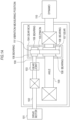
- Fig. 1A is a view for explaining the state of this experiment.
- the state in Fig. 1A is a state where a drive mechanism for a wheel in the railway bogie is placed in a laboratory.
- a drive motor 101 rotates a pinion 105 via a drive motor shaft 102, a gear joint 103, and a pinion shaft 100.
- the pinion 105 rotates, to thereby rotate a gear 107.
- an axle 109 rotates and the wheel connected to the axle 109 rotates eventually.
- a dynamo 110 is connected to the axle 109.
- the dynamo 110 is a generator connected for imparting a pseudo traveling load. In this experiment, the load for rotating the dynamo 110 is assumed as a load when traveling.
- Fig. 1B is a view illustrating a state where the bearings attached to the gear box 104 are seen from the side.
- a position 111 on the gear box 104 is a position where a vibration measuring device is placed.
- the vibration measuring device includes sensors such as an acceleration sensor and a laser displacement sensor, detects vibration of an object through the sensors, and outputs a signal corresponding to the detected vibrations.
- the vibration measuring device placed at the position 111 measures vibrations transmitted to the position 111 and outputs a signal indicating the measured vibrations to an external information processing apparatus and the like through wire or radio communication.
- the vibration measuring device is placed at the position 111, but may be placed at an arbitrary position as long as it is the position where vibrations due to the bearing 106 is transmitted.
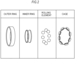
- Fig. 2 is a view explaining one example composition of the bearing 106.
- the bearing 106 is composed of four parts of an outer ring, an inner ring, rolling elements, and a cage.
- Fig. 2 illustrates an outline of the outer ring, the inner ring, the rolling elements, and the cage of the bearing 106.
- the bearing 106 is formed in which the rolling elements held in the cage are sandwiched between the outer ring and the inner ring.
- measured data of the vibrations at the position 111 were acquired in each of the case of the normal bearing 106, the case of the bearing 106 having a flaw in the inner ring, and the case of the bearing 106 having a flaw in the cage.
- the measured data measured by the vibration measuring device are set to measured data y.
- the measured data y was approximated by a revised autoregressive model and from coefficients of the revised autoregressive model, a characteristic amount was calculated.
- a value of the measured data y at a certain time k (1 ⁇ k ⁇ M) is set to y k .
- M is a number indicating a time until when, as the measured data y, data are contained, and is preset.
- the autoregressive model approximating y k is as in Equation 1 below, for example.
- the autoregressive model is, as expressed in Equation 1, an equation expressing a predicted value y ⁇ k of data at the time k (m + 1 ⁇ k ⁇ M) in time-series data (in the equation, ⁇ is illustrated by being added above y) by using an actual value y k - 1 of data at a time k - l (1 ⁇ l ⁇ m) prior to the time in the time-series data.
- Equation 1 ⁇ is a coefficient of the autoregressive model. Further, m is an integer that is less than M, m indicating how many pieces of past data before the time are used to approximate y k being the value of the measured data y at the time k in the autoregressive model, and is set to 1500 in this experiment.
- Equation 2 is a conditional expression for minimizing the square error between the measured data and the predicted value by the autoregressive model.
- Equation 2 The relation of Equation 3 below is satisfied by Equation 2.
- Equation 3 is modified (expressed in matrix notation form), and thereby Equation 4 below is obtained.
- R jl in Equation 4 is called autocorrelation of the measured data y, and is a value defined by Equation 5 below.
- at this time is referred to as a time lag.
- Equation 6 which is a relational expression relating to coefficients of the following autoregressive model, is considered.
- Equation 6 is an equation derived from a condition that minimizes the error between the predicted value of the measured data by the autoregressive model and measured data at the time corresponding to the predicted value, and is called a Yule-Walker equation.
- Equation 6 is a linear equation in which a vector composed of coefficients of the autoregressive model is set to a variable vector, and a constant vector on the left side in Equation 6 is a vector whose component is the autocorrelation of the measured data with a time lag of 1 to m to be referred to as an autocorrelation vector in the following explanation.
- a coefficient matrix on the right side in Equation 6 is a matrix whose component is the autocorrelation of the measured data with a time lag of 0 to m - 1 to be referred to as an autocorrelation matrix in the following explanation.
- Equation 6 a matrix of m ⁇ m composed of R jl .
- the coefficient of the autoregressive model when deriving the coefficient of the autoregressive model, a method of solving a coefficient ⁇ of Equation 6 is used.
- the coefficient ⁇ is derived so as to make the predicted value y ⁇ k of the measured data at the time k derived by the autoregressive model come close to the actual value y k of the measured data at the time k as much as possible. Therefore, the frequency characteristic of the autoregressive model includes a large number of frequency components included in the actual value y k of the measured data at each time.
- the autocorrelation matrix R is subjected to singular value decomposition. Elements of the autocorrelation matrix R are symmetric, and thus when the autocorrelation matrix R is subjected to singular value decomposition, like Equation 8 below, the result becomes the product of an orthogonal matrix U, a diagonal matrix ⁇ , and a transposed matrix of the orthogonal matrix U.
- the matrix ⁇ in Equation 8 is a diagonal matrix whose diagonal component is the eigenvalues of the autocorrelation matrix R as expressed in Equation 9 below.
- the diagonal component of the diagonal matrix ⁇ is set to ⁇ 11 , ⁇ 22 , ⁇ , ( ⁇ mm .
- the matrix U is an orthogonal matrix in which each column component vector is an eigenvector of the autocorrelation matrix R.
- the column component vector of the diagonal matrix U is set to u 1 , u 2 , ⁇ ⁇ ⁇ , u m .
- the eigenvalue of the autocorrelation matrix R responsive to an eigenvector u j is ⁇ jj .
- the eigenvalue of the autocorrelation matrix R is a variable reflecting the strength of each frequency component included in a time waveform of the predicted value of the measured data by the autoregressive model.
- a matrix R' is defined as in Equation 10 below by using, out of these eigenvalues of the autocorrelation matrix R, s pieces of the eigenvalues as the used eigenvalue number being a number set to 1 or more and less than m, which are chosen from the largest.
- the matrix R' is a matrix resulting from approximating the autocorrelation matrix R by using s pieces of the eigenvalues as the used eigenvalue number out of the eigenvalues of the autocorrelation matrix R.
- a matrix U S in Equation 10 is a matrix of m ⁇ s composed of s pieces of the column component vectors, which are chosen from the left of the orthogonal matrix U of Equation 8, (eigenvectors corresponding to the eigenvalues to be used). That is, the matrix U S is a submatrix composed of the left elements of m ⁇ s cut out from the orthogonal matrix U. Further, U S T is a transposed matrix of U S and is a matrix of s ⁇ m composed of s pieces of row component vectors, which are chosen from the top of the matrix U T in Equation 8.
- a matrix ⁇ s in Equation 10 is a matrix of s ⁇ s composed of s pieces of columns, which are chosen from the left, and s pieces of rows, which are chosen from the top, of the diagonal matrix ⁇ in Equation 8. That is, the matrix ⁇ s is a submatrix composed of the top and left elements of s ⁇ s cut out from the diagonal matrix ⁇ .
- Equation 11 When the matrix ⁇ s and the matrix U s are expressed by the matrix elements, Equation 11 below is obtained.
- Equation 12 By using the matrix R' in place of the autocorrelation matrix R, the relational expression of Equation 6 is rewritten into Equation 12 below.
- Equation 12 is modified, and thereby Equation 13 that derives the coefficient ⁇ is obtained.
- the model that calculates the predicted value y ⁇ k from Equation 1 while using the coefficient ⁇ derived by Equation 13 is referred to as the "revised autoregressive model.”
- the matrix U s is not the submatrix composed of the left elements of m ⁇ s cut out from the orthogonal matrix U, but is a submatrix composed of the cut out column component vectors corresponding to the eigenvalues to be used (eigenvectors), and the matrix ⁇ s is not the submatrix composed of the top and left elements of s ⁇ s cut out from the diagonal matrix ⁇ , but is a submatrix to be cut out so as to make the eigenvalues to be used become the diagonal components.
- Equation 13 is an equation to be used for determining the coefficient of the revised autoregressive model.
- the matrix U s in Equation 13 is a third matrix being a matrix in which the eigenvectors corresponding to the eigenvalues to be used are set to the column component vectors, which is the submatrix of the orthogonal matrix obtained by the singular value decomposition of the autocorrelation matrix R.
- the matrix ⁇ s in Equation 13 is a second matrix being a matrix in which the eigenvalues to be used are set to the diagonal components, which is the submatrix of the diagonal matrix obtained by the singular value decomposition of the autocorrelation matrix R.
- the matrix U s ⁇ s U s T in Equation 13 is a first matrix being a matrix derived from the matrix ⁇ s and the matrix U s .
- Equation 13 The right side of Equation 13 is calculated, and thereby the coefficient ⁇ of the revised autoregressive model is derived.
- One example of the method of deriving the coefficient of the revised autoregressive model has been explained above, but deriving the coefficient of the autoregressive model to be the base has been explained by the method of using the least square method for the predicted value in order to make it understandable intuitively.
- the autocorrelation is expressed by autocorrelation of the stochastic process (a population), and this autocorrelation of the stochastic process is expressed as a function of a time lag.
- the autocorrelation of the measured data in this embodiment may be replaced with a value calculated by another calculating formula as long as it approximates the autocorrelation of the stochastic process, and for example, R 22 to R mm are autocorrelation with a time lag of 0, but they may be replaced with R 11 .
- Equation 14 Equation 15 below is obtained.
- Equation 16 a transfer function H(z) being a z-transformation of an impulse response of the system is derived as in Equation 16 below.
- the frequency characteristic of the system appears as changes in amplitude and phase of an output responsive to a sinusoidal input, and is derived by Fourier transform of the impulse response.
- the transfer function H(z) when z is turned on a unit circle of a complex plane results in the frequency characteristic.
- placing z in Equation 16 as in Equation 17 below is considered.
- j denotes an imaginary unit
- ⁇ denotes an angular frequency
- T denotes a sampling interval
- Equation 18 an amplitude characteristic of H(z) (the frequency characteristic of the system) can be expressed like Equation 18 below.
- ⁇ T in Equation 18 is set to vary within a range of 0 to 2 ⁇ .
- the autocorrelation matrix R was derived by using Equation 5 and Equation 7 and was subjected to the singular value decomposition expressed by Equation 8, to thereby derive an eigenvalue of the autocorrelation matrix R, resulting in that the distribution of the eigenvalues of the autocorrelation matrix R was derived. Further, a waveform of the measured data was derived for each of the obtained measured data.
- the matrix ⁇ s and the matrix U s were derived from the singular value decomposition of the autocorrelation matrix R derived by the above procedures by using Equation 11, the coefficient ⁇ of the revised autoregressive model was derived by using Equation 5 and Equation 13, and a waveform of the revised autoregressive model to be specified by the derived coefficient ⁇ was derived. Then, for each of the obtained measured data, the frequency characteristic, and so on of the revised autoregressive model were derived by using Equation 18.
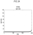
- Fig. 3A to Fig. 3C are views illustrating the distribution of the eigenvalues of the autocorrelation matrix R derived by the above-described procedures on the respective measured data.
- the graph in Fig. 3A is a graph indicating the distribution of the eigenvalues of the autocorrelation matrix R when using the measured data measured in the case where a normal bearing, namely the flawless bearing 106, was used.
- the graph of Fig. 3B is a graph indicating the distribution of the eigenvalues of the autocorrelation matrix R when using the measured data measured in the case where a bearing, namely the bearing 106 having a flaw in the inner ring, was used.
- the graph of Fig. 3C is a graph indicating the distribution of the eigenvalues of the autocorrelation matrix R when using the measured data measured in the case where a bearing, namely the bearing 106 having a flaw in the cage, was used.
- the graphs in Fig. 3A to Fig. 3C each are a graph in which eigenvalues ⁇ 11 to ⁇ mm , which are obtained by subjecting the autocorrelation matrix R to singular value decomposition, are aligned in ascending order and are plotted, and the horizontal axis indicates an index of the eigenvalue and the vertical axis indicates the value of the eigenvalue.
- Seeing Fig. 3A reveals that there are five eigenvalues having a value significantly higher than that of the others. It reveals that particularly, the two eigenvalues out of the five eigenvalues have a value higher than that of the other three eigenvalues.
- Fig. 4A to Fig. 4C are views illustrating waveforms of the respective measured data.
- the graph in Fig. 4A is a graph indicating the waveform of the measured data measured in the case where a normal bearing, namely the flawless bearing 106, was used, and the horizontal axis indicates time and the vertical axis indicates an actual value of the measured data at a corresponding time.
- the graph of Fig. 4B is a graph indicating the waveform of the measured data measured in the case where a bearing, namely the bearing 106 having a flaw in the inner ring, was used, and the horizontal axis indicates time and the vertical axis indicates an actual value of the measured data at a corresponding time.
- the graph of Fig. 4A is a graph indicating the waveform of the measured data measured in the case where a normal bearing, namely the flawless bearing 106, was used, and the horizontal axis indicates time and the vertical axis indicates an actual value of the measured data at a corresponding time.
- the graph of Fig. 4A is a graph indicating the waveform of the measured data measured in the case where
- 4C is a graph indicating the waveform of the measured data measured in the case where a bearing, namely the bearing 106 having a flaw in the cage, was used, and the horizontal axis indicates time and the vertical axis indicates an actual value of the measured data at a corresponding time.
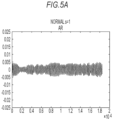
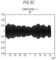
- Fig. 5A to Fig. 5C are views each illustrating a waveform of measured data approximated by a revised autoregressive model specified by the coefficient ⁇ derived by setting the used eigenvalue number s to one.
- the graph in Fig. 5A is a graph indicating the waveform of the measured data approximated by the revised autoregressive model specified by the coefficient a derived from the measured data measured in the case where a normal bearing, namely the flawless bearing 106, was used by setting the used eigenvalue number s to one, and the horizontal axis indicates time and the vertical axis indicates a predicted value of the measured data at a corresponding time.
- the graph in Fig. 5A is a graph indicating the waveform of the measured data approximated by the revised autoregressive model specified by the coefficient a derived from the measured data measured in the case where a normal bearing, namely the flawless bearing 106, was used by setting the used eigenvalue number s to one, and the horizontal axis indicates time and the vertical axis indicates a predicted value of the measured data at a corresponding time.
- 5B is a graph indicating the waveform of the measured data approximated by the revised autoregressive model specified by the coefficient a derived from the measured data measured in the case where a bearing, namely the bearing 106 having a flaw in the inner ring, was used by setting the used eigenvalue number s to one, and the horizontal axis indicates time and the vertical axis indicates a predicted value of the measured data at a corresponding time.
- 5C is a graph indicating the waveform of the measured data approximated by the revised autoregressive model specified by the coefficient ⁇ derived from the measured data measured in the case where a bearing, namely the bearing 106 having a flaw in the cage, was used by setting the used eigenvalue number s to one, and the horizontal axis indicates time and the vertical axis indicates a predicted value of the measured data at a corresponding time.
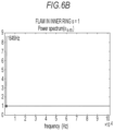
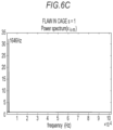
- Fig. 6A to Fig. 6C are views each illustrating a frequency characteristic of the revised autoregressive model specified by the coefficient a derived by setting the used eigenvalue number s to one.
- the graphs in Fig. 6A to Fig. 6C are graphs indicating the frequency characteristics of the respective waveforms of Fig. 5A to Fig. 5C .
- the graph in Fig. 6A is a graph indicating the frequency characteristic, which is derived by Equation 18, of the revised autoregressive model specified by the coefficient ⁇ derived from the measured data measured in the case where a normal bearing, namely the flawless bearing 106, was used by setting the used eigenvalue number s to one, and the horizontal axis indicates frequency and the vertical axis indicates a signal strength.
- the graph in Fig. 6A is a graph indicating the frequency characteristic, which is derived by Equation 18, of the revised autoregressive model specified by the coefficient ⁇ derived from the measured data measured in the case where a normal bearing, namely the flawless bearing 106, was used by setting the used eigenvalue number s to one, and the horizontal axis indicates frequency and the vertical axis indicates a signal strength.
- 6B is a graph indicating the frequency characteristic, which is derived by Equation 18, of the revised autoregressive model specified by the coefficient ⁇ derived from the measured data measured in the case where a bearing, namely the bearing 106 having a flaw in the inner ring, was used by setting the used eigenvalue number s to one, and the horizontal axis indicates frequency and the vertical axis indicates a signal strength.
- 6C is a graph indicating the frequency characteristic, which is derived by Equation 18, of the revised autoregressive model specified by the coefficient ⁇ derived from the measured data measured in the case where a bearing, namely the bearing 106 having a flaw in the cage, was used by setting the used eigenvalue number s to one, and the horizontal axis indicates frequency and the vertical axis indicates a signal strength.
- Seeing the graph in Fig. 6A reveals that a peak rises at a place of the frequency being 824 Hz. Further, seeing the graph in Fig. 6B reveals that a peak rises at a place of the frequency being 1649 Hz. Further, seeing the graph in Fig. 6C reveals that a peak rises at a place of the frequency being 1646 Hz.
- the peak of the frequency characteristic rises at the frequencies similar in value in the case of the bearing 106 having a flaw in the inner ring and the case of the bearing 106 having a flaw in the cage. Therefore, it is possible to judge, from the frequency characteristic of the revised autoregressive model specified by the coefficient ⁇ derived by setting the used eigenvalue number s to one, the presence or absence of a flaw in the inner ring or the cage of the bearing 106, but it is difficult to judge whether the flaw is a flaw in the inner ring, a flaw in the cage, or flaws in the both.
- the value of the used eigenvalue number s was further increased to five, the coefficient ⁇ was derived by using, out of the eigenvalues of the autocorrelation matrix R, the five eigenvalues chosen from the largest, and a waveform and a frequency characteristic of the revised autoregressive model specified by the derived coefficient ⁇ were derived.
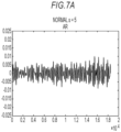
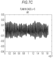
- Fig. 7A to Fig. 7C are views each illustrating a waveform of the revised autoregressive model specified by the coefficient ⁇ derived by setting the used eigenvalue number s to five.
- the graph in Fig. 7A is a graph indicating the waveform of the measured data approximated by the revised autoregressive model specified by the coefficient ⁇ derived from the measured data measured in the case where a normal bearing, namely the flawless bearing 106, was used by setting the used eigenvalue number s to five, and the horizontal axis indicates time and the vertical axis indicates a predicted value of the measured data at a corresponding time.
- the graph in Fig. 7A is a graph indicating the waveform of the measured data approximated by the revised autoregressive model specified by the coefficient ⁇ derived from the measured data measured in the case where a normal bearing, namely the flawless bearing 106, was used by setting the used eigenvalue number s to five, and the horizontal axis indicates time and the vertical axis indicates a predicted value of the measured data at a corresponding time.
- FIG. 7B is a graph indicating the waveform of the measured data approximated by the revised autoregressive model specified by the coefficient ⁇ derived from the measured data measured in the case where a bearing, namely the bearing 106 having a flaw in the inner ring, was used by setting the used eigenvalue number s to five, and the horizontal axis indicates time and the vertical axis indicates a predicted value of the measured data at a corresponding time.
- 7C is a graph indicating the waveform of the measured data approximated by the revised autoregressive model specified by the coefficient ⁇ derived from the measured data measured in the case where a bearing, namely the bearing 106 having a flaw in the cage, was used by setting the used eigenvalue number s to five, and the horizontal axis indicates time and the vertical axis indicates a predicted value of the measured data at a corresponding time.
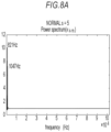
- Fig. 8A to Fig. 8C are views each illustrating a frequency characteristic of the revised autoregressive model specified by the coefficient ⁇ derived by setting the used eigenvalue number s to five.
- the graphs in Fig. 8A to Fig. 8C are graphs indicating the frequency characteristics of the respective waveforms of Fig. 7A to Fig. 7C .
- the graph in Fig. 8A is a graph indicating the frequency characteristic, which is derived by Equation 18, of the revised autoregressive model specified by the coefficient ⁇ derived from the measured data measured in the case where a normal bearing, namely the flawless bearing 106, was used by setting the used eigenvalue number s to five, and the horizontal axis indicates frequency and the vertical axis indicates a signal strength.
- the graph in Fig. 8A is a graph indicating the frequency characteristic, which is derived by Equation 18, of the revised autoregressive model specified by the coefficient ⁇ derived from the measured data measured in the case where a normal bearing, namely the flawless bearing 106, was used by setting the used eigenvalue number s to five, and the horizontal axis indicates frequency and the vertical axis indicates a signal strength.
- FIG. 8B is a graph indicating the frequency characteristic, which is derived by Equation 18, of the revised autoregressive model specified by the coefficient a derived from the measured data measured in the case where a bearing, namely the bearing 106 having a flaw in the inner ring, was used by setting the used eigenvalue number s to five, and the horizontal axis indicates frequency and the vertical axis indicates a signal strength.
- 8C is a graph indicating the frequency characteristic, which is derived by Equation 18, of the revised autoregressive model specified by the coefficient ⁇ derived from the measured data measured in the case where a bearing, namely the bearing 106 having a flaw in the cage, was used by setting the used eigenvalue number s to five, and the horizontal axis indicates frequency and the vertical axis indicates a signal strength.
- Seeing the graph in Fig. 8A reveals that a peak rises at a place of the frequency being 821 Hz and a place of the frequency being 1047 Hz. Further, seeing the graph in Fig. 8B reveals that a peak rises at a place of the frequency being 1648 Hz, a place of the frequency being 2021 Hz, and a place of the frequency being 6474 Hz. Further, seeing the graph in Fig. 8C reveals that a peak rises at a place of the frequency being 1646 Hz, a place of the frequency being 3291 Hz, and a place of the frequency being 1746 Hz.
- the signal strength of the components of the frequencies other than the frequencies where the peak rises in Fig. 6A to Fig. 6C increase at the predicted values by the revised autoregressive model. That is, it is found out that the eigenvalue of the autocorrelation matrix R to be used for deriving the coefficient ⁇ is correlated with the strength of the component of each frequency included in the time waveform of the predicted value of the measured data by the revised autoregressive model specified by the derived coefficient ⁇ .
- the eigenvalues used when deriving the coefficient ⁇ the eigenvalues that are judged as relatively large eigenvalues from such graphs as illustrated in Fig. 3A to Fig. 3C by a user visually may be used, or the eigenvalues that are equal to or more than the average value of the entire eigenvalues, for example, may be used.
- the processing in this embodiment is as follows. That is, based on the findings obtained by this experiment, the autocorrelation matrix R derived from the measured data of vibrations of an object is subjected to singular value decomposition, and by using some of obtained eigenvalues, the coefficient of the revised autoregressive model approximating the measured data is derived. Then, from the revised autoregressive model specified by the derived coefficient, a predicted value of the measured data is not derived by calculating the right side of Equation 1, but a frequency characteristic of the revised autoregressive model is acquired by using the derived coefficient. Then, based on the acquired frequency characteristic, the abnormality of the object is diagnosed. However, processing to derive the predicted value of the measured data (the left side value of Equation 1) may be added to the processing in this embodiment.
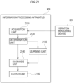
- Fig. 9 is a diagram illustrating one example of a system configuration of the diagnosis system in this embodiment.
- the diagnosis system is a system of performing an abnormality diagnosis of an object that moves periodically.
- the diagnosis system includes an information processing apparatus 900 and a vibration measuring device 901.
- the diagnosis system performs an abnormality diagnosis of a bearing used for a railway bogie.
- the information processing apparatus 900 is an information processing apparatus such as a personal computer (PC), a server device, or a tablet device that performs an abnormality diagnosis of a bearing. Further, the information processing apparatus 900 may be a computer incorporated in an electric railcar or the like.
- the vibration measuring device 901 is a measuring device that includes a sensor such as an acceleration sensor, detects vibrations of the object via the sensor, and outputs a signal according to the detected vibrations to an external apparatus such as the information processing apparatus 900 by wire or radio.
- the information processing apparatus 900 includes an acquisition unit 910, a determination unit 920, a diagnosis unit 930, a judgement unit 940, and an output unit 950.
- the acquisition unit 910 acquires the measured data y relating to the periodical movements of the object that moves periodically.
- the acquisition unit 910 acquires the measured data y of vibrations measured by the vibration measuring device 901 placed at the position 111 when the bearing 106 is rotating.
- the determination unit 920 determines the coefficient ⁇ in the revised autoregressive model based on the measured data y acquired by the acquisition unit 910.
- the determination unit 920 determines the coefficient ⁇ in the revised autoregressive model by using Equation 12 being an equation using a first matrix R' (Equation 10) obtained by extracting the components useful for the abnormality diagnosis of the object from the autocorrelation matrix R in place of the autocorrelation matrix R expressed by Equation 7 in Equation (a Yule-Walker equation) used for determining the coefficients in the autocorrelation matrix that is known generally.
- Equation 12 being an equation using a first matrix R' (Equation 10) obtained by extracting the components useful for the abnormality diagnosis of the object from the autocorrelation matrix R in place of the autocorrelation matrix R expressed by Equation 7 in Equation (a Yule-Walker equation) used for determining the coefficients in the autocorrelation matrix that is known generally.
- Equation 6 is an equation in which the autocorrelation matrix R whose component is the autocorrelation of the measured data y with a time lag of 0 to m - 1 is set to a coefficient matrix and an autocorrelation vector whose component is the autocorrelation of the measured data y with a time lag of 1 to m is set to a constant vector.
- Equation 6 can be derived as a conditional expression that expresses a condition that minimizes a square error between the predicted value y ⁇ k of the measured data y calculated by Equation 1 and the actual measured value y k of the measured data y at the time k corresponding to the predicted value y ⁇ k of the measured data y.
- the first matrix R' is derived from the diagonal matrix ⁇ in which the eigenvalues of the autocorrelation matrix R derived by subjecting the autocorrelation matrix R to the singular value decomposition (Equation 8) are set to diagonal components and the orthogonal matrix U in which eigenvectors of the autocorrelation matrix R are set to column components.
- the first matrix R' is the matrix U s ⁇ s U s T derived from the matrix ⁇ s in which s pieces of the eigenvalues as the used eigenvalue number are set to the diagonal components, which is a submatrix of the diagonal matrix ⁇ , and the matrix U s in which eigenvectors corresponding to s pieces of the eigenvalues as the used eigenvalue number are set to the column component vector, which is a submatrix of the orthogonal matrix U, by using, out of the eigenvalues of the autocorrelation matrix R, s pieces of the eigenvalues as the used eigenvalue number that is set to 1 or more and less than m.
- S pieces of the eigenvalues as the used eigenvalue number may be set to include the eigenvalue having the largest value out of the eigenvalues of the autocorrelation matrix R, but are preferably chosen in descending order of value.
- the determination unit 920 resets the used eigenvalue number s and determines the coefficient ⁇ in the revised autoregressive model again.
- the diagnosis unit 930 diagnoses the abnormality of the object based on the coefficient ⁇ determined by the determination unit 920.
- the diagnosis unit 930 may derive the frequency characteristic exhibiting the distribution of frequencies of the revised autoregressive model from Equation 18 by using the coefficient ⁇ determined by the determination unit 920 to diagnose the abnormality of the object based on this frequency characteristic. Further, the diagnosis unit 930 may regard the presence or absence of the abnormality in the object as a result of the diagnosis or regard the portion having an abnormality in the object as a result of the diagnosis based on the frequency at which a peak is shown in the frequency characteristic.
- the presence or absence of a flaw in the bearing 106 or the portion having a flaw is regarded as a result of the diagnosis.
- the judgement unit 940 judges whether or not the abnormality diagnosis of the object by the diagnosis unit 930 is successful.
- the judgement unit 940 judges the abnormality diagnosis of the object to be unsuccessful, the previously-described determination unit 920 resets the used eigenvalue number s and determines the coefficient ⁇ of the revised autoregressive model again.
- the output unit 950 outputs information relating to the result of the diagnosis by the diagnosis unit 930.
- Fig. 10 is a diagram illustrating one example of a hardware configuration of the information processing apparatus 900.
- the information processing apparatus 900 includes a CPU 1000, a main memory 1001, an auxiliary memory 1002, and an input/output IF 1003. These respective components are connected to be able to communicate to one another through a system bus 1004.
- the CPU 1000 is a central processing unit that controls the information processing apparatus.
- the main memory 1001 is a memory such as a RAM (Random Access Memory) that functions as a work area or a temporary storage location for data of the CPU 1000.
- the auxiliary memory 1002 is a memory such as a ROM (Read Only Memory), a HDD (Hard Disk Drive), or a SSD (Solid State Drive) that stores various programs set data, measured data output from the vibration measuring device 901, diagnosis information, and so on.
- the input/output I/F 1003 is an interface used for exchanging information with an external device such as the vibration measuring device 901.
- the CPU 1000 executes processing based on programs stored in the auxiliary memory 1002 and the like, and thereby the functions of the information processing apparatus 900 explained in Fig. 9 and processing of a flowchart to be explained later in Fig. 11 , and the like are achieved.
- the diagnosis system is set to diagnose the abnormality of the bearing 106 based on measured data of vibrations measured by the vibration measuring device 901 placed at the position 111 under the same state as in Fig. 1 .
- the diagnosis system is set to diagnose the abnormality of the bearing 106 by specifying in which of the portions of the bearing 106 a flaw exists, but may be set to diagnose the abnormality of the bearing 106 by specifying whether or not a flaw exists in the bearing 106.
- the diagnosis system is set to diagnose the abnormality of the bearing 106 based on the measured data measured beforehand by the vibration measuring device 901.
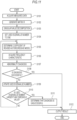
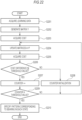
- Fig. 11 is a flowchart illustrating one example of the processing of the information processing apparatus 900.
- the acquisition unit 910 acquires the measured data y of vibrations measured by the vibration measuring device 901.
- the acquisition unit 910 acquires, as the measured data y, y 1 to y M being measured data at a time 1 to a time M.
- the determination unit 920 generates the autocorrelation matrix R by using Equation 5 and Equation 7 based on the measured data y acquired at S1101, a constant M set beforehand, and a number m indicating how many pieces of past data are used to approximate data at a certain time in the revised autoregressive model.
- the determination unit 920 reads pieces of information on M and m stored beforehand, to thereby acquire M and m.
- the value of m is 1500.
- M is an integer larger than m.
- the determination unit 920 subjects the autocorrelation matrix R generated at S1102 to singular value decomposition, to thereby acquire the orthogonal matrix U and the diagonal matrix ⁇ of Equation 8, and acquires the eigenvalues ⁇ 11 to ⁇ mm of the autocorrelation matrix R from the diagonal matrix ⁇ .
- the determination unit 920 sets the used eigenvalue number s, which is the number of eigenvalues of the autocorrelation matrix R to be used for deriving the coefficient ⁇ of the revised autoregressive model, to one.
- the determination unit 920 chooses, out of on to ⁇ mm being the plural eigenvalues of the autocorrelation matrix R, the eigenvalues ⁇ 11 to ⁇ ss from the largest by the used eigenvalue number s as the eigenvalues of the autocorrelation matrix R to be used for deriving the coefficient ⁇ of the revised autoregressive model. Then, the determination unit 920 determines the coefficient ⁇ of the revised autoregressive model by using Equation 13 based on the measured data y, the eigenvalues ⁇ 11 to ⁇ ss , and the orthogonal matrix U obtained by the singular value decomposition of the autocorrelation matrix R.
- the diagnosis unit 930 acquires the frequency characteristic of the revised autoregressive model specified by the coefficient ⁇ determined at S1105 by using Equation 18 based on the coefficient ⁇ determined at S1105.
- the diagnosis unit 930 diagnoses the abnormality of the bearing 106 based on the frequency characteristic acquired at S1106.
- the diagnosis information being information used for the abnormality diagnosis of the bearing 106, which is information indicating correspondence of the frequency at which a peak rises in the frequency characteristic and the state of the bearing 106, is stored in the auxiliary memory beforehand.
- the diagnosis information is information indicating that the bearing 106 is normal as long as the frequency at which a peak rises in the frequency characteristic is within a set range and the bearing 106 has a flaw as long as the frequency at which a peak rises in the frequency characteristic is out of a set range, or the like, for example.
- the diagnosis information may be information indicating the range of the frequency at which a peak rises in the frequency characteristic, which corresponds to the state where the bearing 106 has a flaw in a specific portion, for example.
- the diagnosis information may be information on the threshold value.
- the auxiliary memory 1002 stores the diagnosis information according to the used eigenvalue number beforehand.
- the diagnosis unit 930 acquires the diagnosis information according to the value of the used eigenvalue number s from the auxiliary memory 1002. In this embodiment, the diagnosis unit 930 acquires, as the diagnosis information, correspondence information of a state of the bearing 106 and a range of the frequency at which a peak rises in the frequency characteristic according to the state.
- the diagnosis unit 930 specifies the frequency at which a peak rises based on the frequency characteristic acquired at S1106.
- the diagnosis unit 930 specifies the frequency that is equal to or more than a threshold value in which a signal strength is set as the frequency at which a peak rises from the frequency characteristic acquired at S1106, for example.
- the CPU 1000 may specify, in the case where the frequency specified that a peak rises is consecutive, for example (a peak rises at 100 Hz, 101Hz, and 102Hz, for example), out of these consecutive frequencies, the frequency having the highest signal strength as the frequency at which a peak rises.
- the diagnosis unit 930 diagnoses the abnormality of the bearing 106 based on the specified frequency at which a peak rises and the acquired diagnosis information.
- the diagnosis unit 930 specifies to which of the states of the bearing 106 the specified frequency corresponds based on the correspondence of the state of the bearing 106 indicated by the diagnosis information and the range of the frequency, for example.
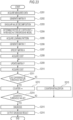
- the judgement unit 940 judges whether or not the abnormality diagnosis is successful based on a diagnosis result at S1107.
- the judgement unit 940 judges the abnormality diagnosis to be successful and the information processing apparatus 900 proceeds to processing at S1112.
- the judgement unit 904 judges the abnormality diagnosis to be unsuccessful and the information processing apparatus 900 proceeds to processing at S1109.
- the determination unit 920 changes the value of the used eigenvalue number s.
- the CPU 1000 sets, for example, a value obtained by adding one to the current value of the used eigenvalue number s as a new value of the used eigenvalue number s.
- the determination unit 920 judges whether or not the value of the used eigenvalue number s is larger than the set threshold value.
- the information processing apparatus 900 proceeds to processing at S1111.
- the determination unit 920 judges the value of the used eigenvalue number s to be equal to or less than the set threshold value
- the information processing apparatus 900 proceeds to processing at S1105.
- the determination unit 920 uses the used eigenvalue number s changed in the value and determines the coefficient ⁇ of the revised autoregressive model again.
- the determination unit 920 judges the abnormality diagnosis of the bearing 106 to be unsuccessful and the information processing apparatus 900 proceeds to processing at S1112.
- the output unit 950 outputs information indicating the result of the abnormality diagnosis of the bearing 106.
- the output unit 950 outputs the information indicating the result of the abnormality diagnosis of the bearing 106 by displaying it on a display device, for example. Further, the output unit 950 may output the information indicating the result of the abnormality diagnosis of the bearing 106 by storing it in the auxiliary memory 1002, for example. Further, the output unit 950 may output the information indicating the result of the abnormality diagnosis of the bearing 106 by transmitting it to a set transmission destination such as an external server device, for example.
- the diagnosis system generates the autocorrelation matrix R from the measured data measured from the periodical movements of the object, subjects the autocorrelation matrix R to the singular value decomposition, and determines the coefficient ⁇ of the revised autoregressive model approximating the measured data by using, out of the obtained eigenvalues, a set number of the eigenvalues chosen from the largest. Then, the diagnosis system derives the frequency characteristic of the revised autoregressive model from the determined coefficient a and diagnoses the abnormality of the bearing 106 based on the derived frequency characteristic.
- the diagnosis system possible to determine the coefficient ⁇ of the revised autoregressive model approximating the measured data so that the component useful for the abnormality diagnosis of the bearing 106 remains and the component unuseful for the abnormality diagnosis of the bearing 106 does not remain. This makes the diagnosis system possible to perform the abnormality diagnosis more accurately based on the component of the measured data useful for the abnormality diagnosis of the bearing 106.
- the processing in this embodiment makes the diagnosis system possible to extract the component useful for the abnormality diagnosis from the measured data without necessity to assume what frequency signal is used for the abnormality diagnosis or the like beforehand.
- the experiment to derive the frequency characteristic of the revised autoregressive model was performed only in the case where the inner ring and the cage out of the parts composing the bearing 106 have a flaw (see Fig. 6A to Fig. 6C and Fig. 8A to Fig. 8C ). Therefore, there is a possibility that accurate detection of the flaw in the rolling element and the flaw in the outer ring fails in the case where a sampling frequency when the acquisition unit 910 acquires the measured data y of the vibrations at S1101 is a frequency higher than the frequencies at which a peak rises at the graphs in Fig. 6A to Fig. 6C and Fig. 8A to Fig. 8C , but frequencies at which a peak rises at graphs of frequency characteristics of a revised autoregressive model in the case where the rolling element and the outer ring have a flaw are higher than this sampling frequency.
- the present inventors further performed the experiment similar to the experiment to diagnose the bearing abnormality explained in the embodiment 1 by using, as the bearing 106, each of a bearing having a flaw in the rolling element and a bearing having a flaw in the outer ring. There will be explained experimental results.
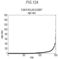
- Fig. 12A and Fig. 12B each are a view illustrating a distribution of eigenvalues of the autocorrelation matrix R similarly to Fig. 3A to Fig. 3C .
- the graph in Fig. 12A is a graph indicating the distribution of eigenvalues of the autocorrelation matrix R when using measured data measured in the case where a bearing, namely the bearing 106 having a flaw in the rolling element, was used.
- the graph in Fig. 12B is a graph indicating the distribution of eigenvalues of the autocorrelation matrix R when using measured data measured in the case where a bearing, namely the bearing 106 having a flaw in the outer ring, was used.
- the graphs in Fig. 12A and Fig. 12B each are a graph in which the eigenvalues ⁇ 11 to ⁇ mm obtained by subjecting the autocorrelation matrix R to singular value decomposition are aligned in ascending order and are plotted, and the horizontal axis indicates an index of the eigenvalue and the vertical axis indicates a value of the eigenvalue.
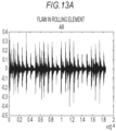
- Fig. 13A and Fig. 13B are views illustrating waveforms of the respective measured data similarly to Fig. 4A to Fig. 4C .
- the graph in Fig. 13A is a graph indicating the waveform of the measured data measured in the case where a bearing, namely the bearing 106 having a flaw in the rolling element, was used, and the horizontal axis indicates time and the vertical axis indicates an actual value of the measured data at a corresponding time.
- the graph of Fig. 13B is a graph indicating the waveform of the measured data measured in the case where a bearing, namely the bearing 106 having a flaw in the outer ring, was used, and the horizontal axis indicates time and the vertical axis indicates an actual value of the measured data at a corresponding time.
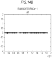
- Fig. 14A and Fig. 14B are views each illustrating a waveform of measured data approximated by a revised autoregressive model specified by the coefficient ⁇ derived by setting the used eigenvalue number s to one similarly to Fig. 5A to Fig. 5C .
- the graph in Fig. 14A is a graph indicating the waveform of the measured data approximated by the revised autoregressive model specified by the coefficient ⁇ derived from the measured data measured in the case where a bearing, namely the bearing 106 having a flaw in the rolling element, was used by setting the used eigenvalue number s to one, and the horizontal axis indicates time and the vertical axis indicates a predicted value of the measured data at a corresponding time.
- the graph in Fig. 14B is a graph indicating the waveform of the measured data approximated by the revised autoregressive model specified by the coefficient a derived from the measured data measured in the case where a bearing, namely the bearing 106 having a flaw in the outer ring, was used by setting the used eigenvalue number s to one, and the horizontal axis indicates time and the vertical axis indicates a predicted value of the measured data at a corresponding time.
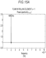
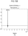
- Fig. 15A and Fig. 15C are views each illustrating a frequency characteristic of the revised autoregressive model specified by the coefficient ⁇ derived by setting the used eigenvalue number s to one similarly to Fig. 6A to Fig. 6C .
- the graphs in Fig. 15A and Fig. 15B are graphs indicating the frequency characteristics of the respective waveforms of Fig. 14A and Fig. 14B .
- the graph in Fig. 15A is a graph indicating the frequency characteristic, which is derived by Equation 18, of the revised autoregressive model specified by the coefficient ⁇ derived from the measured data measured in the case where a bearing, namely the bearing 106 having a flaw in the rolling element, was used by setting the used eigenvalue number s to one, and the horizontal axis indicates frequency and the vertical axis indicates a signal strength.
- the graph in Fig. 15A is a graph indicating the frequency characteristic, which is derived by Equation 18, of the revised autoregressive model specified by the coefficient ⁇ derived from the measured data measured in the case where a bearing, namely the bearing 106 having a flaw in the rolling element, was used by setting the used eigenvalue number s to one, and the horizontal axis indicates frequency and the vertical axis indicates a signal strength.
- 15B is a graph indicating the frequency characteristic, which is derived by Equation 18, of the revised autoregressive model specified by the coefficient ⁇ derived from the measured data measured in the case where a bearing, namely the bearing 106 having a flaw in the outer ring, was used by setting the used eigenvalue number s to one, and the horizontal axis indicates frequency and the vertical axis indicates a signal strength.
- Seeing the graph in Fig. 15A reveals that a peak rises at a place of the frequency being 19853 Hz. Further, seeing the graph in Fig. 15B reveals that a peak rises at a place of the frequency being 23007 Hz.
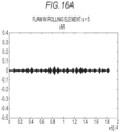
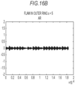
- Fig. 16A and Fig. 16B are views each illustrating a waveform of the revised autoregressive model specified by the coefficient ⁇ derived by setting the used eigenvalue number s to five similarly to Fig. 7A to Fig. 7C .
- the graph in Fig. 16A is a graph indicating the waveform of the measured data approximated by the revised autoregressive model specified by the coefficient ⁇ derived from the measured data measured in the case where a bearing, namely the bearing 106 having a flaw in the rolling element, was used by setting the used eigenvalue number s to five, and the horizontal axis indicates time and the vertical axis indicates a predicted value of the measured data at a corresponding time.
- 16B is a graph indicating the waveform of the measured data approximated by the revised autoregressive model specified by the coefficient ⁇ derived from the measured data measured in the case where a bearing, namely the bearing 106 having a flaw in the outer ring, was used by setting the used eigenvalue number s to five, and the horizontal axis indicates time and the vertical axis indicates a predicted value of the measured data at a corresponding time.
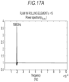
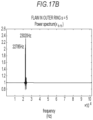
- Fig. 17A and Fig. 17B are views each illustrating a frequency characteristic of the revised autoregressive model specified by the coefficient a derived by setting the used eigenvalue number s to five similarly to Fig. 8A to Fig. 8C .
- the graphs in Fig. 17A and Fig. 17B are graphs indicating the frequency characteristics of the respective waveforms of Fig. 16A and Fig. 16B .
- the graph in Fig. 17A is a graph indicating the frequency characteristic, which is derived by Equation 18, of the revised autoregressive model specified by the coefficient ⁇ derived from the measured data measured in the case where a bearing, namely the bearing 106 having a flaw in the rolling element, was used by setting the used eigenvalue number s to five, and the horizontal axis indicates frequency and the vertical axis indicates a signal strength.
- the graph in Fig. 17A is a graph indicating the frequency characteristic, which is derived by Equation 18, of the revised autoregressive model specified by the coefficient ⁇ derived from the measured data measured in the case where a bearing, namely the bearing 106 having a flaw in the rolling element, was used by setting the used eigenvalue number s to five, and the horizontal axis indicates frequency and the vertical axis indicates a signal strength.
- 17B is a graph indicating the frequency characteristic, which is derived by Equation 18, of the revised autoregressive model specified by the coefficient ⁇ derived from the measured data measured in the case where a bearing, namely the bearing 106 having a flaw in the outer ring, was used by setting the used eigenvalue number s to five, and the horizontal axis indicates frequency and the vertical axis indicates a signal strength.
- Seeing the graph in Fig. 17A reveals that a peak rises at a place of the frequency being 19853 Hz. Further, seeing the graph in Fig. 17B reveals that a peak rises at a place of the frequency being 22785 Hz and a place of the frequency being 23020 Hz.
- the peak at the highest frequency is the peak generated in the vicinity of 23000 Hz in the case where a flaw exists in the outer ring.
- the present inventors learned that a signal having a frequency up to about 7.8 ( ⁇ 23000/2954.7) times as large as the number of rotations of the inner ring is generated in the bearing 106 due to the inner flaw. That is, vibrations relating to rotational movements of the inner ring of the bearing 106 are measured at a sampling frequency at which a peak at 7.8 times the frequency (Hz) of the number of rotations (rpm) of the inner ring of the bearing 106 is detectable, thereby making it possible to detect a flaw generated in each portion of the bearing 106.
- the same processing as that in the embodiment 1 is performed on data relating to the vibrations relating to the rotational movement of the inner ring of the bearing 106 measured at a sampling frequency at which a signal having 7.8 times the frequency (Hz) of the number of rotations (rpm) of the inner ring of the bearing 106 is detectable from the bearing 106 having the inner ring to rotate.
- the system configuration of the diagnosis system in this embodiment is the same as that in the embodiment 1. Further, the hardware configuration and the functional configuration of the information processing apparatus 900 are also the same as those in the embodiment 1.
- the vibration measuring device 901 measures vibrations of the bearing 106 at a sampling frequency at which a signal having 7.8 times the frequency (Hz) of the number of rotations (rpm) of the inner ring of the bearing 106 is detectable.
- the vibration measuring device 901 measures vibrations relating to the rotational movements of the inner ring of the bearing 106 at 15.6 times the sampling frequency (Hz) of the number of rotations (rpm) of the inner ring of the bearing 106 so that, for example, a Nyquist frequency (Hz) increases 7.8 times the number of rotations (rpm) of the inner ring of the bearing 106.
- the vibration measuring device 901 may measure vibrations relating to the rotational movements of the inner ring of the bearing 106 at a sampling frequency (Hz) that is equal to or more than 15.6 times the number of rotations (rpm) of the inner ring of the bearing 106. for example.
- Hz sampling frequency
- the acquisition unit 910 acquires the measured data y of vibrations measured by the vibration measuring device 901 at a sampling frequency at which a signal having 7.8 times the frequency (Hz) of the number of rotations (rpm) of the inner ring of the bearing 106 is detectable.
- the diagnosis system is designed to perform the abnormality diagnosis of the bearing 106 based on the measured data measured at a sampling frequency at which a signal having 7.8 times the frequency (Hz) of the number of rotations (rpm) of the inner ring of the bearing 106 is detectable. This makes the diagnosis system possible to detect a flaw generated in each portion of the bearing 106.
- the diagnosis system generates the autocorrelation matrix R from the measured data measured from the periodical movements of the object, subjects the autocorrelation matrix R to the singular value decomposition, and determines the coefficient ⁇ of the revised autoregressive model approximating the measured data by using, out of the obtained eigenvalues, a set number of the eigenvalues chosen from the largest. Then, the diagnosis system derives the frequency characteristic of the revised autoregressive model from the determined coefficient ⁇ and diagnoses the abnormality of the bearing 106 based on the derived frequency characteristic.
- the autocorrelation matrix R was derived by using Equation 5 and Equation 7 and was subjected to the singular value decomposition expressed by Equation 8, to thereby derive eigenvalues of the autocorrelation matrix R, and a distribution of the eigenvalues of the autocorrelation matrix R was derived.
- the value of m was set to 500.
- Equation 11 the matrix ⁇ s and the matrix U s were derived by using Equation 11
- the coefficient ⁇ of the revised autoregressive model was derived by using Equation 5 and Equation 13.
- the used eigenvalue number s was set to three.
- the state that the bearing 106 can be brought into is set to five states, namely, the flawless normal state, the state of having a flaw in the inner ring, the state of having a flaw in the cage, the state of having a flaw in the rolling element, and the state of having a flaw in the outer ring.
- the number of states that the bearing 106 can be brought into is set to p below. In this experiment, p is five.
- Fig. 18 is a view illustrating patterns of the coefficients a derived by the above-described procedures in each of the case where the bearing 106 is in a normal state, the case where the bearing 106 is in a state of having a flaw in the inner ring, the case where the bearing 106 is in a state of having a flaw in the cage, the case where the bearing 106 is in a state of having a flaw in the rolling element, and the case where the bearing 106 is in a state of having a flaw in the outer ring.
- the pattern of the coefficient a is information indicating a shape formed when components of the coefficient ⁇ are aligned.
- This index i can be regarded as an index indicating a measurement point of the measured data y relating to the components of the coefficient in Equation 1. That is, each of the patterns illustrated in Fig. 18 is one example of the pattern in which the respective components of the coefficient ⁇ are aligned based on the measurement point of the measured data y relating to the respective components in Equation 1.
- Examples of the pattern of the coefficient ⁇ include a vector in which the components of the coefficient ⁇ are aligned in the index order, a vector in which the components of the coefficient ⁇ are aligned in the index order in a manner to skip a predetermined number (for example, one, or the like), a vector in which the components of the coefficient ⁇ are aligned in the order reverse to the indexes, and so on.
- examples of the pattern of the coefficient ⁇ include a vector in which the components of the coefficient a resulting from adding the same value to the respective components are aligned in the index order, a vector in which the components of the coefficient ⁇ resulting from adding the same value to the respective components are aligned in the index order in a manner to skip a predetermined number (for example, one, or the like), a vector in which the components of the coefficient ⁇ resulting from adding the same value to the respective components are aligned in the order reverse to the indexes, and so on.
- a predetermined number for example, one, or the like
- examples of the pattern of the coefficient a include a vector in which the components of the coefficient ⁇ resulting from multiplying the respective components by the same value are aligned in the index order, a vector in which the components of the coefficient a resulting from multiplying the respective components by the same value are aligned in the index order in a manner to skip a predetermined number (for example, one, or the like), a vector in which the components of the coefficient ⁇ resulting from multiplying the respective components by the same value are aligned in the order reverse to the indexes, and so on.
- the pattern of the coefficient ⁇ being the information indicating the shape formed when the components of the coefficient ⁇ are aligned is not a vector but may be an image of a graph in which the components of the coefficient a are aligned.
- each of the patterns of q pieces of the coefficients ⁇ is such a pattern as to show a region surrounded by two vertically symmetrical wavy lines. Further, in the case of the bearing 106 having a flaw in the rolling element, each of the patterns of q pieces of the coefficients ⁇ is a pattern such that a plurality of wavy lines overlap. Further, in the case of the bearing 106 having a flaw in the inner ring, each of the patterns of q pieces of the coefficients ⁇ is a pattern in which a chevron pattern having four peaks is continuous.
- each of the patterns of q pieces of the coefficients ⁇ is a waveform pattern that decays gradually. Further, in the case of the bearing 106 having a flaw in the cage, each of the patterns of q pieces of the coefficients ⁇ is a pattern in which a chevron pattern having two peaks is continuous.
- the coefficient ⁇ of the revised autoregressive model exhibits a characteristic pattern in each of the case of the normal bearing 106, the case of the bearing 106 having a flaw in the inner ring, the case of the bearing 106 having a flaw in the cage, the case of the bearing 106 having a flaw in the rolling element, and the case of the bearing 106 having a flaw in the outer ring.
- a representative pattern of the coefficient ⁇ of the revised autoregressive model was specified by learning in each of the case of the normal bearing 106, the case of the bearing 106 having a flaw in the inner ring, the case of the bearing 106 having a flaw in the cage, the case of the bearing 106 having a flaw in the rolling element, and the case of the bearing 106 having a flaw in the outer ring as below.
- Equation 19 a matrix Y having a size of m ⁇ d that has columns representing the respective coefficients ⁇ illustrated in Fig. 18 is generated like Equation 19 below.
- d is p ⁇ q, and is 250 in this experiment.
- ⁇ k , (i,j) in Equation 19 represents a k-th component ⁇ k of the coefficient ⁇ determined from j-th measured data out of q pieces of measured data measured from the bearing 106 in a state corresponding to i.
- the Y matrix is subjected to non-negative matrix factorization, to thereby specify the representative pattern of the coefficient ⁇ of the revised autoregressive model in each of the states of the bearing 106.
- the components of the matrix Y are each adjusted to a non-negative value by adding the absolute value of the smallest component out of the components that are less than 0 of the matrix Y to each of the components of the matrix Y, for example.
- a matrix whose components are non-negative values is set to a non-negative matrix below.
- the matrix Y is non-negative matrix factorized into a matrix A and a matrix P each being a non-negative value matrix.
- the matrix A is a matrix having a size of m ⁇ p and the matrix P is a matrix having a size of p ⁇ d.
- the number of columns of the matrix A is a base number in the non-negative matrix factorization and is set to p(5) as the number of states that the bearing 106 can be brought into in this embodiment. Thereby, in the columns of the matrix A, patterns of p(5) pieces of the coefficients ⁇ (to be also referred to as bases) derived from the matrix Y are stored.
- a cost function J is defined as in Equation 21 below.
- the right-side first term in Equation 21 represents a condition for making the product of the matrix A and the matrix P and the matrix Y agree with each other in least square meaning.
- the symbol of F at lower right of the right-side first term in Equation 21 is a symbol indicating Frobenius norm. That is, ⁇ AP-Y ⁇ in the right-side first term in Equation 21 is Frobenius norm and results in a square root of the total of squares of the absolute values of components of a matrix (AP-Y).
- the right-side second term in Equation 21 represents a condition requiring a sparse property of the matrix P. Adding this condition makes it possible to prevent overlearning of the non-negative matrix factorization.
- the index i in the right-side second term in Equation 21 is an index indicating a row of a matrix. Further, the index k in the right-side second term in Equation 21 is an index indicating a column of the matrix.
- the right-side third term in Equation 21 represents a condition that approximately requires orthogonality between the patterns stored in different columns in the matrix A, and has an effect of preventing the patterns stored in p(5) pieces of the columns in the matrix A from being linearly dependent as much as possible. If the patterns stored in the columns of the matrix A are linearly dependent, coefficients (to be also referred to as weights) when a certain pattern is approximated by a linear combination of the patterns stored in the columns of the matrix A no longer become a series, and thus identification of the patterns becomes difficult.
- a matrix AT in the right-side third term in Equation 21 is a transposed matrix of the matrix A, and a matrix I is a unit matrix.
- the indexes k, k- (expressed as k with a bar drawn thereabove in Equation) in the right-side third term in Equation 21 are indexes indicating a row and a column of the matrix respectively.
- Equation 21 even when as the cost function J, only the right-side first term in Equation 21 is used, the non-negative matrix factorization functions, and thus as the cost function J, only the right-side first term in Equation 21 may be used. Further, when a problem such as the above-described overlearning or linear dependence occurs, as the cost function J, an equation made by adding the right-side second term and the right-side third term in Equation 21 to the right-side first term in Equation 21 may be used.
- a coefficient ⁇ and a coefficient ⁇ are determined beforehand by a case study, for example, so as to be capable of well associating the respective states of the bearing 106 with learning patterns determined by a method to be described in Fig. 22 , and so on.
- ⁇ is set to 0.035 and ⁇ is set to 0.
- the matrix Y is factorized into the matrix A and the matrix P so as to minimize this cost function J. That is, a minimization problem of the cost function J defined in Equation 22 below is solved.
- a first constraint condition in Equation 22 is a condition expressing that the matrix A and the matrix P are a non-negative matrix.
- a second constraint condition in Equation 22 is a condition for normalizing the matrix A.
- the index k in the second constraint condition in Equation 22 is an index indicating a row and a column of a matrix.
- ⁇ P in Expression 23 is a relaxation coefficient used for updating the matrix P.
- ⁇ A in Expression 24 is a relaxation coefficient used for updating the matrix A.
- Equation 25 A partial differential by the matrix P of the cost function J in Expression 23 is as expressed in Equation 25 below.
- a matrix F in Equation 25 is a matrix that has a size of p ⁇ d and whose components are all one.
- Equation 26 A partial differential by the matrix A of the cost function J in Expression 24 is as expressed in Equation 26 below.
- a matrix E in Equation 26 is a matrix that has a size of p ⁇ p and whose components are all one.
- Equation 23 is rewritten by using Equation 25, to thereby derive Equation 27 below.
- the index i in Equation 27 is an index indicating a row of a matrix.
- the index k in Equation 27 is an index indicating a column of the matrix.
- Equation 27 Since the matrix P is a non-negative matrix, the value of Equation 27 needs to be a non-negative value.
- the right-side third term in Equation 27 is a term to be a non-negative value inevitably. That is, as long as the value of an equation resulting from removing the third term from the right side of Equation 27 is 0, the value of Equation 27 becomes a non-negative value inevitably. Therefore, as expressed in Equation 28, updating the matrix P is performed so as to satisfy the condition that the value of an equation resulting from removing the third term from the right side of Equation 27 is 0.
- the index i in Equation 28 is an index indicating a row of a matrix.
- the index k in Equation 28 is an index indicating a column of the matrix.
- Equation 29 the value of the relaxation coefficient ⁇ P in Expression 23 is derived as in Equation 29 below.
- the index i in Equation 29 is an index indicating a row of a matrix.
- the index k in Equation 29 is an index indicating a column of the matrix.
- the index i in Expression 30 is an index indicating a row of a matrix.
- the index k in Expression 30 is an index indicating a column of the matrix.
- the respective components of the matrix P are updated by using Expression 30, to thereby update the matrix P.
- Equation 24 is rewritten by using Equation 26, to thereby derive Equation 31 below.
- the index k in Equation 31 is an index indicating a row of a matrix.
- the index j in Equation 31 is an index indicating a column of the matrix.
- Equation 31 Since the matrix A is a non-negative matrix, the value of Equation 31 needs to be a non-negative value.
- the right-side third term in Equation 31 is a term to be a non-negative value inevitably. That is, as long as the value of an equation resulting from removing the third term from the right side of Equation 31 is 0, the value of Equation 31 becomes a non-negative value inevitably. Therefore, as expressed in Equation 32 below, updating the matrix A is performed so as to satisfy the condition that the value of an equation resulting from removing the third term from the right side of Equation 31 is 0.
- the index k in Equation 32 is an index indicating a row of a matrix.
- the index j in Equation 32 is an index indicating a column of the matrix.
- Equation 32 the value of the relaxation coefficient ⁇ A in Expression 24 is derived as in Equation 33 below.
- the index k in Equation 33 is an index indicating a row of a matrix.
- the index j in Equation 33 is an index indicating a column of the matrix.
- the index k in Expression 34 is an index indicating a row of a matrix.
- the index j in Expression 34 is an index indicating a column of the matrix.
- the respective components of the matrix A are updated by using Expression 34, to thereby update the matrix A.
- k in Expression 35 is an index indicating a row of a matrix.
- j in Expression 35 is an index indicating a row or a column of the matrix.
- the matrix P is updated by using Expression 30 and updating the matrix A is performed by using Expression 34 and Expression 35 repeatedly.
- the value of the cost function J has converged if the fluctuation in the value of the cost function J continues to be equal to or less than a predetermined threshold value for a predetermined number of times before and after updating the matrix P and the matrix A. Then, the matrix A and the matrix P at this time are set to a matrix to minimize the cost function J.
- Fig. 19 illustrates one example of the patterns exhibited by the columns of the matrix A when the cost function J converged.
- the columns of the matrix A each include m (500) pieces of values and express the patterns of the coefficients ⁇ .
- Fig. 20 illustrates a graph indicating values of the rows of the matrix P when the cost function J converged.
- the horizontal axis of the graph in Fig. 20 indicates an index of the column of the matrix P.
- the vertical axis of the graph in Fig. 20 indicates a value of each component of the matrix P.
- a line 2001 in Fig. 20 is a line connecting d (250) pieces of values of the first row of the matrix P.
- the value is about 12 in a range where the index of the horizontal axis is 0 or more and less than 50 (a range from the first column to the q-th (50th) column), and is a very small value (about 0) in ranges other than this range as compared to the value of 12.
- a line 2002 in Fig. 20 is a line connecting d pieces of values of the second row of the matrix P.
- the value is about 12 in a range where the index of the horizontal axis is 50 or more and less than 100 (a range from the q + 1-th column to the 2q-th column), and is a very small value (about 0) in ranges other than this range as compared to the value of 12.
- a line 2003 in Fig. 20 is a line connecting d pieces of values of the fourth row of the matrix P.
- the value is about 12 in a range where the index of the horizontal axis is 100 or more and less than 150 (a range from the 2q + 1-th column to the 3q-th column), and is a very small value (about 0) in ranges other than this range as compared to the value of 12.
- a line 2004 in Fig. 20 is a line connecting d pieces of values of the fifth row of the matrix P.
- the value is about 12 in a range where the index of the horizontal axis is 150 or more and less than 200 (a range from the 3q + 1-th column to the 4q-th column), and is a very small value (about 0) in ranges other than this range as compared to the value of 12.
- a line 2005 in Fig. 20 is a line connecting d pieces of values of the third row of the matrix P.
- the value is about 12 in a range where the index of the horizontal axis is 200 or more and less than 250 (a range from the 4q + 1-th column to the 5q-th column), and is a very small value (about 0) in ranges other than this range as compared to the value of 12.
- the value of the first row is about 12 and the values of the second to fifth rows are about 0.
- the value of the second row is about 12 and the values of the first row and the third to fifth rows are about 0.
- the value of the fourth row is about 12 and the values of the first to third rows and the fifth row are about 0.
- the value of the fifth row is about 12 and the values of the first to fourth rows are about 0.
- the value of the third row is about 12 and the values of the first, second, fourth, and fifth rows are about 0.
- the patterns exhibited by data of the columns from the first column to the q-th column of the matrix AP are a pattern made by the respective patterns in Fig. 19 being superimposed with a weight of about 12 for the pattern expressed at the top graph in Fig. 19 and a weight of about 0 for the patterns expressed at the graphs other than the top graph in Fig. 19 , and is a pattern similar to the pattern expressed at the top graph in Fig. 19 .
- the patterns exhibited by data of the columns from the q + 1-th column to the 2q-th column of the matrix AP are a pattern made by the respective patterns in Fig. 19 being superimposed with a weight of about 12 for the pattern expressed at the second graph from the top in Fig.
- the patterns exhibited by data of the columns from the 2q + 1-th column to the 3q-th column of the matrix AP are a pattern made by the respective patterns in Fig. 19 being superimposed with a weight of about 12 for the pattern expressed at the second graph from the bottom in Fig. 19 and a weight of about 0 for the patterns expressed at the graphs other than the second graph from the bottom in Fig. 19 , and is a pattern similar to the pattern expressed at the second graph from the bottom in Fig. 19 .
- the patterns exhibited by data of the columns from the 3q + 1-th column to the 4q-th column of the matrix AP are a pattern made by the respective patterns in Fig. 19 being superimposed with a weight of about 12 for the pattern expressed at the bottom graph in Fig. 19 and a weight of about 0 for the patterns expressed at the graphs other than the bottom graph in Fig. 19 , and is a pattern similar to the pattern expressed at the bottom graph in Fig. 19 .
- the patterns exhibited by data of the columns from the 4q + 1-th column to the 5q-th column of the matrix AP are a pattern made by the respective patterns in Fig. 19 being superimposed with a weight of about 12 for the pattern expressed at the third graph from the top in Fig. 19 and a weight of about 0 for the patterns expressed at the graphs other than the third graph from the top in Fig. 19 , and is a pattern similar to the pattern expressed at the third graph from the top in Fig. 19 .
- the patterns exhibited by data of the columns from the first column to the q-th column of the matrix Y are a pattern corresponding to the bearing 106 having a flaw in the outer ring illustrated in Fig. 18 .
- the patterns exhibited by data of the columns from the q + 1-th column to the 2q-th column of the matrix Y are a pattern corresponding to the bearing 106 having a flaw in the rolling element illustrated in Fig. 18 .
- the patterns exhibited by data of the columns from the 2q + 1-th column to the 3q-th column of the matrix Y are a pattern corresponding to the bearing 106 having a flaw in the inner ring illustrated in Fig. 18 .
- the patterns exhibited by data of the columns from the 3q + 1-th column to the 4q-th column of the matrix Y are a pattern corresponding to the flawless normal bearing 106 illustrated in Fig. 18 .
- the patterns exhibited by data of the columns from the 4q + 1-th column to the 5q-th column of the matrix Y are a pattern corresponding to the bearing 106 having a flaw in the cage illustrated in Fig. 18 .
- a comparison between the matrix Y and the matrix A reveals that the patterns exhibited by the data of the columns of the matrix Y and the patterns exhibited by the data of the columns of the matrix A are similar. That is, it reveals that the patterns exhibited by the data of the columns of the matrix A are the patterns of the coefficients ⁇ that correspond to the bearings 106 in the respective states respectively.
- the data of the first column of the matrix A exhibit the representative pattern of the coefficient ⁇ corresponding to the bearing 106 in a state of having a flaw in the outer ring.
- the data of the second column of the matrix A exhibit the representative pattern of the coefficient a corresponding to the bearing 106 in a state of having a flaw in the rolling element.
- the data of the third column of the matrix A exhibit the representative pattern of the coefficient ⁇ corresponding to the bearing 106 in a state of having a flaw in the cage.
- the data of the fourth column of the matrix A exhibit the representative pattern of the coefficient ⁇ corresponding to the bearing 106 in a state of having a flaw in the inner ring.
- the data of the fifth column of the matrix A exhibit the representative pattern of the coefficient ⁇ corresponding to the bearing 106 in a flawless normal state.
- the processing in this embodiment is the following processing. That is, measured data of vibrations of the bearing 106 are acquired beforehand with respect to the bearing 106 in each of the state of having a flaw in the outer ring, the state of having a flaw in the rolling element, the state of having a flaw in the inner ring, the flawless normal state, and the state of having a flaw in the cage, and regarding each of the acquired measured data, the autocorrelation matrix R derived from the measured data is subjected to singular value decomposition, and by using some of the obtained eigenvalues, the coefficient of the revised autoregressive model approximating the measured data is derived.
- the matrix Y being each of the coefficients derived from the data of the columns is generated and the generated matrix Y is learned by non-negative matrix factorization, to thereby specify the patterns of the coefficients in the revised autoregressive models that correspond to the bearings 106 in the respective states.
- the measured data of vibrations of the bearing 106 to be a target for abnormality diagnosis is acquired, the autocorrelation matrix R derived from the acquired measured data is subjected to singular value decomposition, and by using some of the obtained eigenvalues, the coefficient of the revised autoregressive model approximating the measured data is derived.
- the processing is to diagnose the abnormality of the bearing 106 based on the pattern of the derived coefficient and the pattern of the coefficient specified by learning.
- Fig. 21 is a diagram illustrating one example of a system configuration of the diagnosis system in this embodiment.
- the diagnosis system is a system of performing an abnormality diagnosis of an object that moves periodically similarly to the embodiment 1.
- the diagnosis system includes an information processing apparatus 900 and a vibration measuring device 901 similarly to the embodiment 1.
- the diagnosis system performs the abnormality diagnosis of a bearing used for a railway bogie.
- a hardware configuration of the information processing apparatus 900 is the same as that in the embodiment 1.
- the CPU 1000 in the information processing apparatus 900 executes processing based on programs stored in the auxiliary memory 1002 and the like, and thereby functions of the information processing apparatus 900 illustrated in Fig. 21 , processing of flowcharts to be described later in Fig. 22 and Fig. 23 , and so on are achieved.
- the information processing apparatus 900 includes an acquisition unit 2110, a determination unit 2120, a learning unit 2130, a diagnosis unit 2140, and an output unit 2150.
- the acquisition unit 910 acquires measured data y relating to periodical movements of an object that moves periodically similarly to the acquisition unit 910 in Fig. 9 .
- the determination unit 2120 determines a coefficient ⁇ in a revised autoregressive model based on the measured data y acquired by the acquisition unit 2110 similarly to the determination unit 920 in Fig. 9 .
- the learning unit 2130 sets coefficients ⁇ in revised autoregressive models determined by the determination unit 2120 from measured data of objects in a plurality of states that are acquired by the acquisition unit 2110 beforehand as learning data and specifies patterns of the coefficients ⁇ in the revised autoregressive models that correspond to the objects in a plurality of states respectively by learning.
- the patterns specified by learning of the learning unit 2130 are set as learning patterns below.
- the diagnosis unit 2140 diagnoses the abnormality of the object based on the coefficient ⁇ determined by the determination unit 2120 and the patterns of the coefficients in the revised autoregressive models in the respective states of the object that are specified by learning of the learning unit 2130.
- the diagnosis unit 2140 subjects, for example, the coefficient ⁇ determined by the determination unit 2120 to non-negative matrix factorization by using the learning patterns and diagnosis the abnormality of the object based on weights of the respective learning patterns of the coefficient ⁇ determined by the determination unit 2120.
- the state of the bearing 106 is set as a result of the diagnosis.
- the output unit 2150 outputs information relating to the result of the diagnosis by the diagnosis unit 2140 similarly to the output unit 950 in Fig. 9 .
- the diagnosis system diagnoses the abnormality of the bearing 106 based on the measured data of vibrations measured by the vibration measuring device 901 placed at the position 111 under the same state as that in Fig. 1A and Fig. 1B .
- Fig. 22 is a flowchart illustrating one example of the learning processing. There will be explained processing to specify the learning pattern by learning while using Fig. 22 .
- the information processing apparatus 900 performs the following processing for q (50) times repeatedly beforehand in each of the case where the bearing 106 is in a state of having a flaw in the outer ring, the case where the bearing 106 is in a state of having a flaw in the rolling element, the case where the bearing 106 is in a state of having a flaw in the inner ring, the case where the bearing 106 is in a flawless normal state, and the case where the bearing 106 is in a state of having a flaw in the cage.
- the acquisition unit 2110 acquires the measured data y of vibrations measured by the vibration measuring device 901.
- the acquisition unit 2110 acquires, as the measured data y, y1 to yM being measured data at times 1 to M in the case where the time set randomly is set to the time 1.
- the determination unit 2120 generates the autocorrelation matrix R by using Equation 5 and Equation 7 based on the measured data y acquired at S2301, a constant M set beforehand, and a number m indicating how many pieces of past data are used to approximate data at a certain time in the revised autoregressive model.
- the determination unit 2120 reads pieces of information on M and m stored beforehand, to thereby acquire M and m.
- the value of m is 500.
- M is an integer larger than m.
- the determination unit 2120 subjects the generated autocorrelation matrix R to singular value decomposition, to thereby acquire the orthogonal matrix U and the diagonal matrix ⁇ of Equation 8, and acquires the eigenvalues ⁇ 11 to ⁇ mm of the autocorrelation matrix R from the diagonal matrix ⁇ .
- the determination unit 2120 chooses, out of ⁇ 11 to ⁇ mm being the plural eigenvalues of the autocorrelation matrix R, the eigenvalues ⁇ 11 to ⁇ ss from the largest by the used eigenvalue number s as the eigenvalues of the autocorrelation matrix R to be used for deriving the coefficient ⁇ of the revised autoregressive model.
- the used eigenvalue number s is set to three, but may be two or less or four or more.
- the determination unit 2120 determines the coefficient ⁇ of the revised autoregressive model by using Equation 13 based on the measured data y, the eigenvalues ⁇ 11 to ⁇ ss , and the orthogonal matrix U obtained by the singular value decomposition of the autocorrelation matrix R. Then, the determination unit 2120 makes the determined coefficient ⁇ non-negative (for example, adds a value obtained by multiplying the lowest value of the component contained in the coefficient ⁇ , which is less than 0, by -1 to the respective components of the coefficient ⁇ , or the like) to be stored in the auxiliary memory 1002 as the learning data.
- the information processing apparatus 900 can acquire, as the learning data, q (50) pieces of data of the coefficient ⁇ in the revised autoregressive model in each of the case where the bearing 106 is in a state of having a flaw in the outer ring, the case where the bearing 106 is in a state of having a flaw in the rolling element, the case where the bearing 106 is in a state of having a flaw in the inner ring, the case where the bearing 106 is in a flawless normal state, and the case where the bearing 106 is in a state of having a flaw in the cage and store them.
- the state that the bearing 106 can be brought into is set to five states, namely, the flawless normal state, the state of having a flaw in the inner ring, the state of having a flaw in the cage, the state of having a flaw in the rolling element, and the state of having a flaw in the outer ring. That is, the number of states that the bearing 106 can be brought into p is five.
- the learning unit 2130 acquires the learning data stored in the auxiliary memory 1002.
- the learning unit 2130 generates the matrix Y of Expression 23 based on the learning data acquired at S2201.
- the learning unit 2130 generates the matrix Y by generating a matrix having a size of m(500) ⁇ d(250) and setting data of columns to values of the respective coefficients ⁇ contained in the learning data. Further, the learning unit 2130 generates the matrix A having a size of m ⁇ p and sets a predetermined initial value to respective components of the matrix A. Further, the learning unit 2130 generates the matrix P having a size of p ⁇ d and sets a predetermined initial value to respective components of the matrix P.
- the learning unit 2130 derives the value of the cost function J as a cost by using Equation 21 based on the matrix Y, the matrix A, and the matrix P that are generated at S2202, a predetermined coefficient ⁇ , and a predetermined coefficient ⁇ .
- the learning unit 2130 stores the derived cost in the main memory 1001 and the like as a cost before updating.
- the learning unit 2130 updates the matrix A by using Expression 34 based on the matrix Y, the matrix A, the matrix P, the coefficient ⁇ , and the matrix E being a matrix that has a size of p ⁇ p and whose components are all one. Further, the learning unit 2130 further updates the updated matrix A by using Expression 35. Further, the learning unit 2130 updates the matrix P by using Expression 30 based on the matrix Y, the matrix A, the matrix P, the coefficient ⁇ , and the matrix F being a matrix that has a size of m ⁇ p and whose components are all one.
- the learning unit 2130 derives the value of the cost function J as a cost by using Equation 21 based on the matrix Y, the matrix A updated at S2203, the matrix P updated at S2203, the coefficient ⁇ , and the coefficient ⁇ .
- the learning unit 2130 stores the derived cost in the main memory 1001 and the like as a cost after updating.
- the learning unit 2130 judges whether or not the absolute value of the difference between the cost after updating and the cost before updating is a predetermined threshold value or less. When judging that the absolute value of the difference between the cost after updating and the cost before updating is the predetermined threshold value or less, the learning unit 2130 proceeds to processing at S2207. Further, when judging that the absolute value of the difference between the cost after updating and the cost before updating is larger than the predetermined threshold value, the learning unit 2130 proceeds to processing at S2208. The learning unit 2130 stores the cost after updating in the main memory 1001 as a new cost before updating after the processing at S2206.
- the learning unit 2130 adds one to a value of a counter stored in the main memory 1001 or the like.
- the learning unit 2130 initializes the value of the counter to 0 before the processing in Fig. 22 starts.
- the learning unit 2130 initializes the value of the counter stored in the main memory 1001 or the like to 0 and proceeds to processing at S2204.
- the learning unit 2130 judges whether or not the value of the counter stored in the main memory 1001 or the like is a predetermined threshold value or more. When judging that the value of the counter stored in the main memory 1001 or the like is the predetermined threshold value or more, the learning unit 2130 regards that the value of the cost function J has converged to a minimum value and proceeds to processing at S2210. When judging that the value of the counter stored in the main memory 1001 or the like is less than the predetermined threshold value, the learning unit 2130 proceeds to processing at S2204.
- the learning unit 2130 specifies, based on the matrix P, which of the patterns of the coefficients ⁇ in the revised autoregressive models corresponding to the bearings 106 in the respective states the patterns exhibited by the data of the columns of the matrix A are.
- the data of a certain column of the matrix Y are derived as data obtained by multiplying the matrix A and the column of the matrix P together. That is, the data of a certain column of the matrix Y result in data obtained by superimposition of the data of the columns of the matrix A with values of rows at the column of the matrix P set as weights.
- the learning unit 2130 specifies which of the patterns of the coefficients ⁇ in the revised autoregressive models corresponding to the bearings 106 in the respective states the patterns exhibited by the data of the columns of the matrix A are in the following manner.
- the learning unit 2130 specifies, out of the columns of the matrix Y, the column in which the data indicating the coefficient ⁇ that corresponds to the bearing 106 in a certain state are to be stored. For example, the learning unit 2130 specifies, out of the columns of the matrix Y, the first column to the q-th column, each of which is the column in which the data indicating the coefficient ⁇ that corresponds to the bearing 106 in a state of having a flaw in the outer ring are to be stored. Then, the learning unit 2130 totalizes the values of the specified columns (the first column to the q-th column) in the matrix P for each row. Then, the learning unit 2130 specifies the row corresponding to the largest value out of the totalized values.
- the learning unit 2130 specifies the column of the matrix A to be multiplied by the specified row of the matrix P.
- the learning unit 2130 specifies the first column because the column of the matrix A to be multiplied by the first row of the matrix P is the first column.
- the learning unit 2130 specifies the data indicated by the specified column of the matrix A as the data exhibiting the representative pattern of the coefficient ⁇ corresponding to the bearing 106 in the state.
- the learning unit 2130 performs the above processing in each of the states that the bearing 106 can be brought into, to thereby specify which of the patterns of the coefficients a in the revised autoregressive models corresponding to the bearings 106 in the respective states the patterns exhibited by the data of the columns of the matrix A are.
- the learning unit 2130 stores the data exhibiting the specified representative patterns of the coefficients ⁇ in the revised autoregressive models corresponding to the bearings 106 in the respective states in the auxiliary memory 1002 or the like as the learning patterns.
- the diagnosis system specifies where in the bearing 106 a flaw exists, to thereby diagnose the abnormality of the bearing 106, but may diagnose the abnormality of the bearing 106 by specifying whether or not a flaw exists in the bearing 106.
- the diagnosis system may diagnose the abnormality of the bearing 106 based on the measured data measured by the vibration measuring device 901 beforehand, or may also diagnose the abnormality of the bearing 106 in operation by using measured data continuously measured by the vibration measuring device 901 in real time to be output.
- Fig. 23 is a flowchart illustrating one example of the abnormality diagnosis processing.
- the acquisition unit 2110 acquires the measured data y of vibrations measured by the vibration measuring device 901.
- the acquisition unit 2110 acquires, as the measured data y, y1 to yM being measured data at the times 1 to M.
- the determination unit 2120 generates the autocorrelation matrix R by using Equation 5 and Equation 7 based on the measured data y acquired at S2301, the constant M set beforehand, and the number m indicating how many pieces of past data are used to approximate data at a certain time in the revised autoregressive model.
- the determination unit 2120 reads pieces of information on M and m stored beforehand, to thereby acquire M and m.
- the value of m is 500.
- M is an integer larger than m.
- the determination unit 2120 subjects the autocorrelation matrix R generated at S2302 to singular value decomposition, to thereby acquire the orthogonal matrix U and the diagonal matrix ⁇ of Equation 8, and acquires the eigenvalues ⁇ 11 to ⁇ mm of the autocorrelation matrix R from the diagonal matrix ⁇ .
- the determination unit 2120 chooses, out of ⁇ 11 to ⁇ mm being the plural eigenvalues of the autocorrelation matrix R, the eigenvalues ⁇ 11 to ⁇ ss from the largest by the used eigenvalue number s as the eigenvalues of the autocorrelation matrix R to be used for deriving the coefficient ⁇ of the revised autoregressive model.
- the used eigenvalue number s is set to three, but may be two or less or four or more.
- the determination unit 2120 determines the coefficient ⁇ of the revised autoregressive model by using Equation 13 based on the measured data y, the eigenvalues ⁇ 11 to ⁇ ss , and the orthogonal matrix U obtained by the singular value decomposition of the autocorrelation matrix R.
- the coefficient ⁇ determined at S2304 is one example of revision coefficients being the coefficients in the revised autoregressive model determined from the measured data.
- the pattern of the coefficient ⁇ determined at S2304 is one example of measurement patterns.
- the diagnosis unit 2140 acquires the learning pattern specified finally at S2304 from the auxiliary memory 1002.
- the diagnosis unit 2140 generates the matrix Y having a size of m ⁇ d like Equation 19 by using the coefficient ⁇ determined at S2304 with d set to one. That is, one column of the matrix Y exhibits the pattern of the coefficient ⁇ determined at S2304. Further, the diagnosis unit 2140 makes components of the matrix Y non-negative (for example, adds a value obtained by multiplying the lowest of the components of the matrix Y, which is less than 0, by -1 to the respective components of the matrix Y, or the like).
- the diagnosis unit 2140 generates the matrix A having a size of m ⁇ p. Then, the diagnosis unit 2140 sets the data of the learning pattern in the columns of the matrix A. Further, the diagnosis unit 2140 generates the matrix P having a size of p ⁇ d(1) and sets a predetermined initial value in its components. The diagnosis unit 2140 updates the matrix P with the value of the matrix A generated at S2307 set as a fixed value, to thereby subject the matrix Y to non-negative matrix factorization.
- the diagnosis unit 2140 derives the value of the cost function J as a cost by using Equation 21 based on the matrix Y, the matrix A, the matrix P, the predetermined coefficient ⁇ , and the predetermined coefficient ⁇ .
- the diagnosis unit 2140 stores the derived cost in the main memory 1001 and the like as a cost before updating.
- the diagnosis unit 2140 updates the matrix P by using Expression 30 based on the matrix Y, the matrix A, the matrix P, the coefficient ⁇ , and the matrix F being a matrix that has a size of m ⁇ p and whose components are all one.
- the diagnosis unit 2140 derives the value of the cost function J as a cost by using Equation 21 based on the matrix Y, the matrix A, the matrix P updated at S2309, the coefficient ⁇ , and the coefficient ⁇ .
- the diagnosis unit 2140 stores the derived cost in the main memory 1001 and the like as a cost after updating.
- the diagnosis unit 2140 judges whether or not the absolute value of the difference between the cost after updating and the cost before updating is a predetermined threshold value or less. When judging that the absolute value of the difference between the cost after updating and the cost before updating is the predetermined threshold value or less, the diagnosis unit 2140 proceeds to processing at S2312. Further, when judging that the absolute value of the difference between the cost after updating and the cost before updating is larger than the predetermined threshold value, the diagnosis unit 2140 proceeds to processing at S2313. The diagnosis unit 2140 stores the cost after updating in the main memory 1001 as a new cost before updating after the processing at S2311.
- the diagnosis unit 2140 adds one to the value of the counter stored in the main memory 1001 or the like.
- the diagnosis unit 2140 initializes the value of the counter to 0 before the processing in Fig. 23 starts.
- the diagnosis unit 2140 initializes the value of the counter stored in the main memory 1001 or the like to 0 and proceeds to processing at S2309.
- the diagnosis unit 2140 judges whether or not the value of the counter stored in the main memory 1001 or the like is a predetermined threshold value or more. When judging that the value of the counter stored in the main memory 1001 or the like is the predetermined threshold value or more, the diagnosis unit 2140 regards that the value of the cost function J has converged to a minimum value and proceeds to processing at S2315. When judging that the value of the counter stored in the main memory 1001 or the like is less than the predetermined threshold value, the diagnosis unit 2140 proceeds to processing at S2309.
- the diagnosis unit 2140 diagnoses the state of the bearing 106 based on the matrix P.
- the diagnosis unit 2140 specifies the row corresponding to the largest out of the values of the rows of the matrix P, for example.
- the diagnosis unit 2140 specifies the column of the matrix A to be multiplied by the specified row of the matrix P. Then, the diagnosis unit 2140 diagnoses that the state of the bearing 106 is brought into a state corresponding to the learning pattern exhibited by the specified column of the matrix A.
- diagnosis unit 2140 may diagnose that the state of the bearing 106 is brought into the state corresponding to the learning pattern exhibited by the specified column of the matrix A by specifying the row corresponding to, out of the values of the rows of the matrix P, the value that is equal to or more than the predetermined threshold value and specifying the column of the matrix A to be multiplied by the specified row of the matrix P.
- the diagnosis unit 2140 may specify a plurality of the columns of the matrix A to be multiplied by a plurality of the specified rows and diagnose that the state of the bearing 106 is brought into a combined state of a plurality of the states corresponding to the learning patterns exhibited by a plurality of the specified columns of the matrix A. Further, in the case where, for example, the matrix P does not include in the rows the values that are equal to or more than the predetermined threshold value, the diagnosis unit 2140 may diagnose the bearing 106 as being in an unknown state (for example, a state where an unknown abnormality occurs).
- the output unit 2150 outputs information indicating the result of the abnormality diagnosis of the bearing 106 at S2315.
- the output unit 2150 outputs the information indicating the result of the abnormality diagnosis of the bearing 106 by displaying it on a display device, for example. Further, the output unit 2150 may output the information indicating the result of the abnormality diagnosis of the bearing 106 by storing it in the auxiliary memory 1002, for example. Further, the output unit 2150 may output the information indicating the result of the abnormality diagnosis of the bearing 106 by transmitting it to a set transmission destination such as an external server device, for example.
- the diagnosis system beforehand generates the autocorrelation matrix R from the measured data measured from the periodical movements of the bearings 106 in a plurality of states, subjects the autocorrelation matrix R to the singular value decomposition, and determines, as the learning data, the coefficient ⁇ of the revised autoregressive model approximating the measured data by using, out of the obtained eigenvalues, a set number of the eigenvalues chosen from the largest. Then, the diagnosis system uses the learning data to specify, as the learning pattern, the representative patterns of the coefficients a corresponding to the bearings 106 in the respective states by learning.
- the diagnosis system determines the coefficient ⁇ of the revised autoregressive model from the measured data measured from the periodical movements of the bearing 106 to be a target for diagnosis and diagnoses the abnormality of the bearing 106 based on the pattern of the determined coefficient ⁇ and the learning pattern specified by learning.
- the diagnosis system possible to determine the coefficient ⁇ of the revised autoregressive model approximating the measured data so that the component useful for the abnormality diagnosis of the bearing 106 remains and the component unuseful for the abnormality diagnosis of the bearing 106 does not remain.
- the experiment reveals that a characteristic pattern is exhibited in each of the states of the bearing 106, and in this embodiment, the diagnosis system diagnoses the abnormality of the bearing 106 based on the pattern of the coefficient ⁇ . This makes the diagnosis system possible to perform the abnormality diagnosis more accurately based on the component of the measured data useful for the abnormality diagnosis of the bearing 106.
- the diagnosis system is designed to perform the abnormality diagnosis of the bearing 106 in the railway bogie.
- the diagnosis system may be designed to perform an abnormality diagnosis of another object that moves periodically, namely, a rotating body such as a gear, an oscillating body such as an oscillator, an elastic body such as a spring, a heart of a creature, or the like.
- m is set to a preset number of 1500. Further, in the embodiment 3, m is set to a number of 500. However, it is also possible to specify the number of past data capable of appropriately approximating the measured data by performing an experiment according to a target to be diagnosed or the like and set the specified number to the value of m.
- the information processing apparatus 900 may, regarding measured data measured from the target to be diagnosed, approximate the measured data at a certain time by using a plurality of past measured data before the time and using an autocorrelation model or the like and determine, as m, the number of the past measured data used for the approximation in the case where the difference between the approximated value and the measured data at the time is less than a set threshold value.
- the information processing apparatus 900 is designed to set the initial value of the used eigenvalue number s to one and change the value of the used eigenvalue number s when failing in the abnormality diagnosis. Further, in the embodiment 3, the information processing apparatus 900 sets the used eigenvalue number s to three. However, the information processing apparatus 900 may determine the value of the used eigenvalue number s as follows. That is, the information processing apparatus 900 first derives the total value of all the eigenvalues of the autocorrelation matrix R.
- the information processing apparatus 900 may determine, as the used eigenvalue number s, the smallest out of a pieces of the eigenvalues, the total of a pieces of the eigenvalues, which are chosen from the largest, out of the eigenvalues of the autocorrelation matrix R being equal to or more than a set percentage of the derived total value (for example, 90%).
- the information processing apparatus 900 is designed to determine the coefficient ⁇ in the revised autoregressive model by using, out of the eigenvalues of the autocorrelation matrix R, s pieces of the eigenvalues as the used eigenvalue number, which are chosen from the largest.
- the information processing apparatus 900 may be designed to determine the coefficient ⁇ in the revised autoregressive model by using, out of the eigenvalues of the autocorrelation matrix R, s pieces of the arbitrary eigenvalues.
- the information processing apparatus 900 may be designed to determine the coefficient ⁇ in the revised autoregressive model by using, out of the eigenvalues of the autocorrelation matrix R, two of the largest eigenvalue and the third-largest eigenvalue.
- the diagnosis system is designed to diagnose the abnormality of the bearing 106 based on the measured data measured by the vibration measuring device 901 beforehand.
- the diagnosis system may be designed to diagnose the abnormality of the bearing 106 in operation by using measured data continuously measured by the vibration measuring device 901 in real time to be output. That is, the information processing apparatus 900 may be designed to update the measured data y 1 to y M every time the new measured data y are acquired from the vibration measuring device 901 and perform the processing in Fig. 11 or Fig. 23 .
- the embodiment 3 includes the direct correspondences between the learning patterns obtained from the learning data by the non-negative matrix factorization and the respective states. That is, when the patterns of the coefficients ⁇ corresponding to the bearings 106 in the respective states are approximated by the linear combination of the learning patterns, the weights concentrate in the learning patterns corresponding to the respective states. However, even when such concentrations of the weights applied to the learning patterns are not seen, the linear combination of the learning patterns using the weights only needs to be derived newly again as the learning patterns corresponding to the respective states as long as correspondences between the combinations of the weights applied to the learning patterns and the patterns of the coefficients ⁇ corresponding to the bearings 106 in the respective states exist.
- the diagnosis system is designed to specify five pieces of the patterns representing the coefficient ⁇ in the revised autoregressive model by learning in the case where the bearing 106 is in each of the five states.
- the diagnosis system may be designed to specify six or more patterns representing the coefficient ⁇ in the revised autoregressive model by learning in each of the states of the bearing 106.
- the learning unit 2130 generates the matrix Y by using Equation 19 with the value of p set to a value of six or more, for example, and updates the matrix A having a size of m ⁇ p and the matrix P having a size of p ⁇ d so as to minimize the cost function J, to thereby specify the patterns of the coefficients ⁇ corresponding to the bearings 106 in the respective states by learning as the columns of the matrix A.
- the learning unit 2130 may be designed to perform the following processing.
- the learning unit 2130 may set the coefficients ⁇ in the revised autoregressive models determined from measured data acquired from the bearings 106 in the respective states as learning data to specify patterns of nine pieces of the coefficients ⁇ corresponding to the bearings 106 in the respective states by learning.
- the diagnosis system may be designed to specify four or less patterns representing the coefficient ⁇ in the revised autoregressive model by learning in each of the states of the bearing 106.
- the learning unit 2130 generates the matrix Y by using Equation 19 with the value of p set to a value of four or less, for example, and updates the matrix A having a size of m ⁇ p and the matrix P having a size of p ⁇ d so as to minimize the cost function J, to thereby specify the patterns of the coefficients ⁇ corresponding to the bearings 106 in the respective states by learning as the columns of the matrix A.
- the learning unit 2130 may set the coefficients ⁇ in the revised autoregressive models determined from measured data acquired from the bearings 106 in the both states as learning data to specify patterns of two pieces of the coefficients ⁇ corresponding to the bearings 106 in the both states by learning.
- the diagnosis system diagnoses the abnormality by specifying in which of the predetermined five states (the flawless normal state, the state of having a flaw in the outer ring, the state of having a flaw in the inner ring, the state of having a flaw in the rolling element, and the state of having a flaw in the cage) the bearing 106 is.
- the diagnosis system may use, out of the learning patterns, only the learning pattern corresponding to the bearing 106 in the normal state and perform the following processing, to thereby diagnose whether or not the bearing 106 is normal.
- the diagnosis system updates, out of the components of the matrix A, the components of the columns other than the column in which the learning pattern corresponding to the bearing 106 in the flawless normal state is stored by using Expression 34. Then, as long as the value of the row of the matrix P to be multiplied by the column in which the learning pattern corresponding to the bearing 106 in the flawless normal state is stored out of the components of the matrix A is the largest among the values of the rows of the matrix P at S2315, the diagnosis system may be designed to diagnose the bearing 106 as being in the normal state.
- the diagnosis system may diagnose the abnormality of the bearing 106 by using a part of the learning patterns specified by learning.
- each q pieces of the coefficients ⁇ in the revised autoregressive models determined from the measured data corresponding to the bearings 106 in the plural states are stored with respect to each state.
- the coefficients ⁇ in the revised autoregressive models determined from the measured data corresponding to the bearings 106 in the plural states may be stored in different numbers with respect to each state.
- the diagnosis system generates the matrix Y so as to make the columns each storing the coefficient ⁇ corresponding to the bearing 106 in the same state continuous.
- the diagnosis system may generate the matrix Y so as not to make the columns each storing the coefficient ⁇ corresponding to the bearing 106 in the same state continuous.
- the diagnosis system generates the matrix Y including the columns having the coefficients ⁇ corresponding the bearings 106 in the respective states stored therein and learns the matrix Y by the non-negative matrix factorization, to thereby specify the representative patterns of the coefficients a corresponding to the bearings 106 in the respective states.
- the diagnosis system may determine a plurality of the coefficients ⁇ corresponding to the bearing 106 in a certain state by the processing similar to that performed when acquiring the learning data, for example, and perform learning by deriving the average of the determined plural coefficients ⁇ , to thereby specify the pattern exhibited by the derived average coefficient as the representative pattern of the coefficient a corresponding to the bearing 106 in the state.
- the diagnosis system diagnoses the abnormality of the bearing 106 based on the pattern of the coefficient ⁇ in the revised autoregressive model determined from the measured data of the bearing 106.
- the diagnosis system may derive the frequency characteristic of the revised autoregressive model by using Equation 18, for example, to diagnose the abnormality of the bearing 106 based on the derived frequency characteristic.
- the diagnosis system may be designed to perform the processing in Fig. 23 when the diagnosis system derives the frequency characteristic of the revised autoregressive model by using Equation 18, for example, and diagnoses the abnormality of the bearing 106 based on the derived frequency characteristic, ending in failure in the diagnosis.
- the diagnosis system diagnoses the abnormality based on the pattern of the coefficient ⁇ in the revised autoregressive model determined from the measured data of the bearing 106 and the frequency characteristic of the revised autoregressive model determined from the measured data of the bearing 106, to thereby enable more accurate diagnosis of the abnormality of the bearing 106.
- the information processing apparatus 900 is designed to perform the processing in Fig. 11 , Fig. 22 , and Fig. 23 by executing the programs stored in the auxiliary memory 1002.
- the information processing apparatus 900 may be designed to perform the processing in Fig. 11 , Fig. 22 , and Fig. 23 by executing the programs stored in an external storage medium, an external storage server, or the like.
- the functions of the above-described information processing apparatus 900 may be mounted in the information processing apparatus 900 as a hardware.
Landscapes
- Physics & Mathematics (AREA)
- General Physics & Mathematics (AREA)
- Acoustics & Sound (AREA)
- Testing Of Devices, Machine Parts, Or Other Structures Thereof (AREA)
- Measurement Of Mechanical Vibrations Or Ultrasonic Waves (AREA)
- Complex Calculations (AREA)
Claims (16)
- Appareil de traitement d'informations (900, 2110) de diagnostic d'anomalie d'un roulement (106), comprenant :un moyen d'acquisition (910, 2120) qui acquiert des données mesurées relatives à des vibrations du roulement (106) ;un moyen de détermination (920, 2130) qui détermine, sur la base des données mesurées acquises par le moyen d'acquisition, un coefficient de révision qui est un coefficient dans un modèle autorégressif révisé ; etun moyen de diagnostic (930, 2140) qui diagnostique une anomalie du roulement (106) sur la base du coefficient de révision déterminé par le moyen de détermination ; etun moyen de sortie (950, 2150) qui délivre en sortie des informations relatives au résultat du diagnostic par le moyen de diagnostic, dans lequelle modèle autorégressif révisé est une équation exprimant une valeur prédite des données mesurées en utilisant une valeur réelle des données mesurées et le coefficient de révision en réponse à la valeur réelle,le moyen de détermination détermine le coefficient de révision en utilisant une équation dans laquelle une première matrice est définie sur une matrice de coefficients et un vecteur d'autocorrélation dérivé des données mesurées est défini sur un vecteur constant, où la première matrice est dérivée d'une matrice diagonale et d'une matrice orthogonale, la matrice diagonale est une matrice dont la composante diagonale est constituée de valeurs propres d'une matrice d'autocorrélation, les valeurs propres étant dérivées en soumettant la matrice d'autocorrélation dérivée des données mesurées à une décomposition en valeurs singulières, et la matrice orthogonale est une matrice dans laquelle un vecteur propre de la matrice d'autocorrélation est défini sur une composante de colonne,le vecteur d'autocorrélation est un vecteur dont la composante est l'autocorrélation des données mesurées avec un retard temporel de 1 à m, m étant un nombre de la valeur réelle utilisée dans le modèle autorégressif révisé,la matrice d'autocorrélation est une matrice dont la composante est l'autocorrélation des données mesurées avec un retard temporel de 0 à m - 1,la première matrice est une matrice USΣSUS T qui est dérivée d'une deuxième matrice ΣS dérivée de s fragments des valeurs propres de la matrice d'autocorrélation, s étant un nombre défini sur 1 ou plus et moins que m, et de la matrice diagonale et d'une troisième matrice Us dérivée de s fragments des valeurs propres et de la matrice orthogonale,la deuxième matrice est une sous-matrice de la matrice diagonale et est une matrice dont la composante diagonale est constituée de s fragments des valeurs propres, etla troisième matrice est une sous-matrice de la matrice orthogonale et est une matrice dans laquelle les vecteurs propres correspondant à s fragments des valeurs propres sont définis sur un vecteur de composante de colonne.
- Appareil de traitement d'informations selon la revendication 1, dans lequel
s fragments des valeurs propres incluent la valeur propre ayant la plus grande valeur parmi les valeurs propres de la matrice d'autocorrélation. - Appareil de traitement d'informations selon la revendication 2, dans lequel
s fragments des valeurs propres sont des valeurs propres qui sont choisies parmi les valeurs propres de la matrice d'autocorrélation dans l'ordre décroissant de valeur. - Appareil de traitement d'informations selon l'une quelconque des revendications 1 à 3, comprenant en outre :un moyen de jugement (940) qui juge si le diagnostic d'anomalie du roulement (106) par le moyen de diagnostic est réussi ou non, dans lequelle moyen de détermination réinitialise s et détermine le coefficient de révision à nouveau lorsque le moyen de jugement juge que le diagnostic d'anomalie du roulement (106) par le moyen de diagnostic n'est pas réussi, etlorsque le moyen de jugement juge que le diagnostic d'anomalie du roulement (106) par le moyen de diagnostic n'est pas réussi, le moyen de diagnostic diagnostique en outre l'anomalie du roulement (106) sur la base du coefficient de révision déterminé à nouveau par le moyen de détermination.
- Appareil de traitement d'informations selon l'une quelconque des revendications 1 à 4, dans lequel
la matrice d'autocorrélation est une matrice incluse dans une expression conditionnelle qui exprime une condition rendant minimale une erreur quadratique entre une valeur prédite des données mesurées et une valeur mesurée réelle des données mesurées à un instant correspondant à la valeur prédite des données mesurées. - Appareil de traitement d'informations selon l'une quelconque des revendications 1 à 5, dans lequel
le moyen de diagnostic dérive une caractéristique de fréquence indiquant une distribution de fréquence du modèle autorégressif révisé en utilisant le coefficient de révision déterminé par le moyen de détermination, et diagnostique l'anomalie du roulement (106) sur la base de la caractéristique de fréquence. - Appareil de traitement d'informations selon la revendication 6, dans lequel
le moyen de diagnostic spécifie la présence ou l'absence de l'anomalie du roulement (106) sur la base d'une fréquence à laquelle un pic est représenté dans la caractéristique de fréquence et définit un résultat obtenu par la spécification comme étant un résultat de diagnostic, pour ainsi diagnostiquer l'anomalie du roulement (106). - Appareil de traitement d'informations selon la revendication 6 ou 7, dans lequel
le moyen de diagnostic spécifie une partie, du roulement (106), ayant une anomalie sur la base d'une fréquence à laquelle un pic est représenté dans la caractéristique de fréquence et définit un résultat obtenu par la spécification comme étant un résultat de diagnostic, pour ainsi diagnostiquer l'anomalie du roulement (106). - Appareil de traitement d'informations selon l'une quelconque des revendications 1 à 5, dans lequel
le moyen de diagnostic diagnostique l'anomalie du roulement (106) sur la base d'un schéma de mesure qui est un schéma du coefficient de révision déterminé par le moyen de détermination. - Appareil de traitement d'informations selon la revendication 9, comprenant en outre :un moyen d'apprentissage (2130) qui spécifie, sur la base de données d'apprentissage qui sont un ou plusieurs coefficients dans le modèle autorégressif révisé déterminé à partir du roulement (106) dans chacun d'une pluralité d'états prédéterminés, un schéma du coefficient dans le modèle autorégressif révisé correspondant à chacun d'une pluralité des états par apprentissage en tant que schéma d'apprentissage, dans lequelle moyen de diagnostic diagnostique l'anomalie du roulement (106) sur la base du schéma de mesure déterminé par le moyen de détermination et le schéma d'apprentissage spécifié par le moyen d'apprentissage par apprentissage.
- Appareil de traitement d'informations selon la revendication 10, dans lequel
le moyen d'apprentissage soumet une matrice qui inclut des colonnes ayant chacune les données d'apprentissage stockées en leur sein à une factorisation matricielle non négative avec le nombre d'une pluralité des états défini sur un nombre de base, pour ainsi spécifier le schéma d'apprentissage par apprentissage. - Appareil de traitement d'informations selon l'une quelconque des revendications 1 à 11, dans lequelle roulement (106) est un roulement destiné à être utilisé dans un bogie ferroviaire, etle moyen de diagnostic diagnostique une anomalie incluant la présence d'un défaut dans le roulement (106) sur la base du coefficient de révision déterminé par le moyen de détermination.
- Appareil de traitement d'informations selon la revendication 12, dans lequelles vibrations du roulement (106) sont des vibrations basées sur des mouvements de rotation d'une bague interne dans le roulement (106), etles données mesurées sont des données mesurées à une fréquence d'échantillonnage (Hz) qui est égale ou supérieure à 15,6 fois le nombre de rotations (tr/min) de la bague interne du roulement.
- Système de diagnostic, comprenantun dispositif de mesure de vibrations (901), etun appareil de traitement d'informations (900) selon l'une quelconque des revendications précédentes, dans lequel l'appareil de traitement d'informations (900) est configuré pour acquérir les données mesurées provenant du dispositif de mesure de vibrations (901).
- Procédé de traitement d'informations devant être exécuté par un appareil de traitement d'informations de diagnostic d'anomalie d'un roulement (106), le procédé comprenant :une étape d'acquisition qui acquiert des données mesurées relatives à des vibrations du roulement (106) ;une étape de détermination qui détermine, sur la base des données mesurées acquises par l'étape d'acquisition, un coefficient de révision qui est un coefficient dans un modèle autorégressif révisé ;une étape de diagnostic qui diagnostique une anomalie du roulement (106) sur la base du coefficient de révision déterminé par l'étape de détermination ; etune étape de sortie qui délivre en sortie des informations relatives au résultat du diagnostic par l'étape de diagnostic, dans lequelle modèle autorégressif révisé est une équation exprimant une valeur prédite des données mesurées en utilisant une valeur réelle des données mesurées et le coefficient de révision en réponse à la valeur réelle,l'étape de détermination détermine le coefficient de révision en utilisant une équation dans laquelle une première matrice est définie sur une matrice de coefficients et un vecteur d'autocorrélation dérivé des données mesurées est défini sur un vecteur constant, où la première matrice est dérivée d'une matrice diagonale et d'une matrice orthogonale, la matrice diagonale est une matrice dont la composante diagonale est constituée de valeurs propres d'une matrice d'autocorrélation, les valeurs propres étant dérivées en soumettant la matrice d'autocorrélation dérivée des données mesurées à une décomposition en valeurs singulières, et la matrice orthogonale est une matrice dans laquelle un vecteur propre de la matrice d'autocorrélation est défini sur une composante de colonne,le vecteur d'autocorrélation est un vecteur dont la composante est l'autocorrélation des données mesurées avec un retard temporel de 1 à m, m étant un nombre de la valeur réelle utilisée dans le modèle autorégressif révisé,la matrice d'autocorrélation est une matrice dont la composante est l'autocorrélation des données mesurées avec un retard temporel de 0 à m - 1,la première matrice est une matrice USΣSUS T qui est dérivée d'une deuxième matrice ΣS dérivée de s fragments des valeurs propres de la matrice d'autocorrélation, s étant un nombre défini sur 1 ou plus et moins que m, et de la matrice diagonale et d'une troisième matrice Us dérivée de s fragments des valeurs propres et de la matrice orthogonale,la deuxième matrice est une sous-matrice de la matrice diagonale et est une matrice dont la composante diagonale est constituée de s fragments des valeurs propres, etla troisième matrice est une sous-matrice de la matrice orthogonale et est une matrice dans laquelle les vecteurs propres correspondant à s fragments des valeurs propres sont définis sur un vecteur de composante de colonne.
- Programme d'ordinateur pour diagnostic d'anomalie d'un roulement (106), comprenant des instructions qui, lorsque le programme est exécuté par un ordinateur, amènent l'ordinateur à exécuter les étapes comprenant :une étape d'acquisition qui acquiert des données mesurées relatives à des vibrations du roulement (106) ;une étape de détermination qui détermine, sur la base des données mesurées acquises par l'étape d'acquisition, un coefficient de révision qui est un coefficient dans un modèle autorégressif révisé ;une étape de diagnostic qui diagnostique une anomalie du roulement (106) sur la base du coefficient de révision déterminé par l'étape de détermination ; etune étape de sortie qui délivre en sortie des informations relatives au résultat du diagnostic par l'étape de diagnostic, dans lequelle modèle autorégressif révisé est une équation exprimant une valeur prédite des données mesurées en utilisant une valeur réelle des données mesurées et le coefficient de révision en réponse à la valeur réelle,l'étape de détermination détermine le coefficient de révision en utilisant une équation dans laquelle une première matrice est définie sur une matrice de coefficients et un vecteur d'autocorrélation dérivé des données mesurées est défini sur un vecteur constant, où la première matrice est dérivée d'une matrice diagonale et d'une matrice orthogonale, la matrice diagonale est une matrice dont la composante diagonale est constituée de valeurs propres d'une matrice d'autocorrélation, les valeurs propres étant dérivées en soumettant la matrice d'autocorrélation dérivée des données mesurées à une décomposition en valeurs singulières, et la matrice orthogonale est une matrice dans laquelle un vecteur propre de la matrice d'autocorrélation est défini sur une composante de colonne,le vecteur d'autocorrélation est un vecteur dont la composante est l'autocorrélation des données mesurées avec un retard temporel de 1 à m, m étant un nombre de la valeur réelle utilisée dans le modèle autorégressif révisé,la matrice d'autocorrélation est une matrice dont la composante est l'autocorrélation des données mesurées avec un retard temporel de 0 à m -1,la première matrice est une matrice USΣSUS T qui est dérivée d'une deuxième matrice ΣS dérivée de s fragments des valeurs propres de la matrice d'autocorrélation, s étant un nombre défini sur 1 ou plus et moins que m, et de la matrice diagonale et d'une troisième matrice Us dérivée de s fragments des valeurs propres et de la matrice orthogonale,la deuxième matrice est une sous-matrice de la matrice diagonale et est une matrice dont la composante diagonale est constituée de s fragments des valeurs propres, etla troisième matrice est une sous-matrice de la matrice orthogonale et est une matrice dans laquelle les vecteurs propres correspondant à s fragments des valeurs propres sont définis sur un vecteur de composante de colonne.
Applications Claiming Priority (3)
| Application Number | Priority Date | Filing Date | Title |
|---|---|---|---|
| JP2017151727A JP6919397B2 (ja) | 2017-03-24 | 2017-08-04 | 情報処理装置、情報処理方法及びプログラム |
| JP2017206597A JP6848813B2 (ja) | 2017-10-25 | 2017-10-25 | 情報処理装置、情報処理方法及びプログラム |
| PCT/JP2018/028942 WO2019026980A1 (fr) | 2017-08-04 | 2018-08-01 | Dispositif de traitement d'informations, procédé de traitement d'informations et programme |
Publications (4)
| Publication Number | Publication Date |
|---|---|
| EP3663741A1 EP3663741A1 (fr) | 2020-06-10 |
| EP3663741A4 EP3663741A4 (fr) | 2021-05-19 |
| EP3663741C0 EP3663741C0 (fr) | 2024-11-06 |
| EP3663741B1 true EP3663741B1 (fr) | 2024-11-06 |
Family
ID=65232868
Family Applications (1)
| Application Number | Title | Priority Date | Filing Date |
|---|---|---|---|
| EP18840775.3A Active EP3663741B1 (fr) | 2017-08-04 | 2018-08-01 | Dispositif de traitement d'informations, procédé de traitement d'informations et programme |
Country Status (5)
| Country | Link |
|---|---|
| EP (1) | EP3663741B1 (fr) |
| JP (1) | JP6848813B2 (fr) |
| CN (1) | CN110998272A (fr) |
| ES (1) | ES2995833T3 (fr) |
| WO (1) | WO2019026980A1 (fr) |
Families Citing this family (11)
| Publication number | Priority date | Publication date | Assignee | Title |
|---|---|---|---|---|
| WO2021117752A1 (fr) * | 2019-12-11 | 2021-06-17 | Ntn株式会社 | Procédé de surveillance d'état de palier à roulement et dispositif de surveillance d'état de palier à roulement |
| JP7242595B2 (ja) * | 2020-02-26 | 2023-03-20 | 株式会社東芝 | 学習装置、推論装置、学習方法及び推論方法 |
| EP4201800A4 (fr) | 2020-08-24 | 2024-10-02 | Furuno Electric Co., Ltd. | Dispositif d'aide à la navigation d'embarcation, procédé d'aide à la navigation d'embarcation et programme d'aide à la navigation d'embarcation |
| CN115551779A (zh) * | 2020-08-24 | 2022-12-30 | 古野电气株式会社 | 船舶航行支援装置、船舶航行支援方法以及船舶航行支援程序 |
| WO2022059719A1 (fr) * | 2020-09-15 | 2022-03-24 | 国立大学法人京都大学 | Système de diagnostic de structure, nœud de capteur, procédé de diagnostic de structure et programme de diagnostic de structure |
| JP7469828B2 (ja) * | 2020-09-15 | 2024-04-17 | 株式会社 日本構造分析舎 | 構造物診断システム、構造物診断方法、および構造物診断プログラム |
| KR102900438B1 (ko) * | 2020-10-27 | 2025-12-15 | 제이에프이 스틸 가부시키가이샤 | 이상 진단 모델의 구축 방법, 이상 진단 방법, 이상 진단 모델의 구축 장치 및 이상 진단 장치 |
| JP7610112B2 (ja) * | 2021-03-09 | 2025-01-08 | 日本製鉄株式会社 | 圧延機のスピンドルの異常診断装置、方法及びプログラム |
| CN113899550B (zh) * | 2021-09-28 | 2022-08-02 | 新黎明科技股份有限公司 | 迭代高阶能量算子融合防爆电机轴承故障诊断方法及系统 |
| JP7788947B2 (ja) * | 2022-06-14 | 2025-12-19 | 三菱電機株式会社 | 車両検査システム、車両検査方法、および車両検査プログラム |
| CN116558828B (zh) * | 2023-07-10 | 2023-09-15 | 昆明理工大学 | 基于自相关系数稀疏度特征的滚动轴承健康状态评估方法 |
Family Cites Families (14)
| Publication number | Priority date | Publication date | Assignee | Title |
|---|---|---|---|---|
| JPS57127820A (en) * | 1981-01-30 | 1982-08-09 | Sumitomo Metal Ind Ltd | Method of monitoring cyclically moving body |
| JP3108405B2 (ja) * | 1998-07-23 | 2000-11-13 | 核燃料サイクル開発機構 | 機器の診断方法 |
| JP4471543B2 (ja) * | 2001-08-06 | 2010-06-02 | 三井造船株式会社 | 周期的運動体の異常診断方法および装置 |
| BR0203292A (pt) * | 2002-08-14 | 2004-05-18 | Michitoshi Oishi | Detetor de defeitos das máquinas rotativas |
| JP5535954B2 (ja) * | 2011-01-28 | 2014-07-02 | 三菱重工業株式会社 | 健全性評価装置及びその方法並びにプログラム |
| JP6196093B2 (ja) * | 2012-12-25 | 2017-09-13 | Ntn株式会社 | 軸受装置の振動解析方法、軸受装置の振動解析装置、および転がり軸受の状態監視装置 |
| EP3029449A4 (fr) * | 2013-08-01 | 2017-03-15 | NTN Corporation | Procédé et dispositif d'analyse de vibration de dispositif à palier, et dispositif de surveillance d'état de palier de roulement |
| CN104655425B (zh) * | 2015-03-06 | 2017-05-03 | 重庆大学 | 基于稀疏表示和大间隔分布学习的轴承故障分类诊断方法 |
| CN105021399B (zh) * | 2015-06-26 | 2017-12-05 | 长安大学 | 一种基于单通道信号盲分离滚动轴承的特征提取方法 |
| CN105300692B (zh) * | 2015-08-07 | 2017-09-05 | 浙江工业大学 | 一种基于扩展卡尔曼滤波算法的轴承故障诊断及预测方法 |
| CN105606363B (zh) * | 2016-01-29 | 2017-11-07 | 济南大学 | 一种基于域自适应的轴承故障诊断方法 |
| CN105806604B (zh) * | 2016-03-18 | 2018-10-19 | 北京唐智科技发展有限公司 | 一种机车车辆走行部轴承保持架故障预报警方法 |
| CN106895975B (zh) * | 2017-01-17 | 2019-03-15 | 苏州大学 | 基于Stacked SAE深度神经网络的轴承故障诊断方法 |
| CN106885697B (zh) * | 2017-03-17 | 2019-09-20 | 华东交通大学 | 基于fcm-hmm的滚动轴承的性能退化评估方法 |
-
2017
- 2017-10-25 JP JP2017206597A patent/JP6848813B2/ja active Active
-
2018
- 2018-08-01 ES ES18840775T patent/ES2995833T3/es active Active
- 2018-08-01 EP EP18840775.3A patent/EP3663741B1/fr active Active
- 2018-08-01 WO PCT/JP2018/028942 patent/WO2019026980A1/fr not_active Ceased
- 2018-08-01 CN CN201880052067.6A patent/CN110998272A/zh active Pending
Also Published As
| Publication number | Publication date |
|---|---|
| WO2019026980A1 (fr) | 2019-02-07 |
| EP3663741C0 (fr) | 2024-11-06 |
| EP3663741A4 (fr) | 2021-05-19 |
| JP2019079352A (ja) | 2019-05-23 |
| JP6848813B2 (ja) | 2021-03-24 |
| CN110998272A (zh) | 2020-04-10 |
| EP3663741A1 (fr) | 2020-06-10 |
| ES2995833T3 (en) | 2025-02-11 |
Similar Documents
| Publication | Publication Date | Title |
|---|---|---|
| EP3663741B1 (fr) | Dispositif de traitement d'informations, procédé de traitement d'informations et programme | |
| CN110370649B (zh) | 3d打印设备的在线监测装置、系统 | |
| Cross et al. | Features for damage detection with insensitivity to environmental and operational variations | |
| Favarelli et al. | Machine learning for automatic processing of modal analysis in damage detection of bridges | |
| CN116380445B (zh) | 基于振动波形的设备状态诊断方法及相关装置 | |
| CN114342003B (zh) | 传感器无关的机械机器故障识别 | |
| JP6919397B2 (ja) | 情報処理装置、情報処理方法及びプログラム | |
| US20190146036A1 (en) | Rotor diagnostic apparatus, rotor diagnostic method, and rotor diagnostic program | |
| JP6580532B2 (ja) | 歯車装置のかみ合い状態推定方法およびプログラム | |
| WO2005015332A2 (fr) | Systeme et procede de surveillance de charge virtuelle | |
| JP7036233B2 (ja) | 情報処理装置、情報処理方法及びプログラム | |
| Er et al. | Approach towards sensor placement, selection and fusion for real-time condition monitoring of precision machines | |
| Mendrok et al. | Operational modal filter and its applications | |
| CN119474783A (zh) | 一种印刷设备维护用的检查测试方法及装置 | |
| Yabe et al. | Characteristics of a bridge condition assessment method based on state representation methodology (SRM) and damage detection sensitivity | |
| Tibaduiza et al. | Structural Health Monitoring based on principal component analysis: damage detection, localization and classification | |
| Sun et al. | Adaptive fault components extraction based on physically interpretable optimized weight time–frequency matrix index and its applications in rotating machinery fault diagnosis | |
| Bilski et al. | Rough-sets-based reduction for analog systems diagnostics | |
| Cheng et al. | Detecting damage to offshore platform structures using the time-domain data | |
| Güneş | Unsupervised learning approach for detection and localization of structural damage using output-only measurements | |
| Vazquez et al. | Fault diagnosis approach for pedelec drive units based on support vector machines | |
| Stricker et al. | Efficient simulative pass/fail characterization applied to automotive power steering | |
| García-Palacios et al. | Uncertainty optimization of automated operational modal analysis applied to structural health monitoring techniques | |
| Raman et al. | Sensor-fault tolerant condition monitoring of an industrial machine | |
| BAHEDH | Online Multi Sensing and Faults Prognosis of Rotating Machinery Using Intelligent Approaches |
Legal Events
| Date | Code | Title | Description |
|---|---|---|---|
| STAA | Information on the status of an ep patent application or granted ep patent |
Free format text: STATUS: THE INTERNATIONAL PUBLICATION HAS BEEN MADE |
|
| PUAI | Public reference made under article 153(3) epc to a published international application that has entered the european phase |
Free format text: ORIGINAL CODE: 0009012 |
|
| STAA | Information on the status of an ep patent application or granted ep patent |
Free format text: STATUS: REQUEST FOR EXAMINATION WAS MADE |
|
| 17P | Request for examination filed |
Effective date: 20200304 |
|
| AK | Designated contracting states |
Kind code of ref document: A1 Designated state(s): AL AT BE BG CH CY CZ DE DK EE ES FI FR GB GR HR HU IE IS IT LI LT LU LV MC MK MT NL NO PL PT RO RS SE SI SK SM TR |
|
| AX | Request for extension of the european patent |
Extension state: BA ME |
|
| DAV | Request for validation of the european patent (deleted) | ||
| DAX | Request for extension of the european patent (deleted) | ||
| A4 | Supplementary search report drawn up and despatched |
Effective date: 20210416 |
|
| RIC1 | Information provided on ipc code assigned before grant |
Ipc: G01M 13/04 20190101AFI20210412BHEP Ipc: G01H 17/00 20060101ALI20210412BHEP Ipc: G01H 13/00 20060101ALI20210412BHEP Ipc: G01M 13/045 20190101ALI20210412BHEP |
|
| STAA | Information on the status of an ep patent application or granted ep patent |
Free format text: STATUS: EXAMINATION IS IN PROGRESS |
|
| 17Q | First examination report despatched |
Effective date: 20230206 |
|
| GRAP | Despatch of communication of intention to grant a patent |
Free format text: ORIGINAL CODE: EPIDOSNIGR1 |
|
| STAA | Information on the status of an ep patent application or granted ep patent |
Free format text: STATUS: GRANT OF PATENT IS INTENDED |
|
| INTG | Intention to grant announced |
Effective date: 20231211 |
|
| GRAJ | Information related to disapproval of communication of intention to grant by the applicant or resumption of examination proceedings by the epo deleted |
Free format text: ORIGINAL CODE: EPIDOSDIGR1 |
|
| STAA | Information on the status of an ep patent application or granted ep patent |
Free format text: STATUS: EXAMINATION IS IN PROGRESS |
|
| INTC | Intention to grant announced (deleted) | ||
| GRAP | Despatch of communication of intention to grant a patent |
Free format text: ORIGINAL CODE: EPIDOSNIGR1 |
|
| STAA | Information on the status of an ep patent application or granted ep patent |
Free format text: STATUS: GRANT OF PATENT IS INTENDED |
|
| INTG | Intention to grant announced |
Effective date: 20240605 |
|
| GRAS | Grant fee paid |
Free format text: ORIGINAL CODE: EPIDOSNIGR3 |
|
| GRAA | (expected) grant |
Free format text: ORIGINAL CODE: 0009210 |
|
| STAA | Information on the status of an ep patent application or granted ep patent |
Free format text: STATUS: THE PATENT HAS BEEN GRANTED |
|
| AK | Designated contracting states |
Kind code of ref document: B1 Designated state(s): AL AT BE BG CH CY CZ DE DK EE ES FI FR GB GR HR HU IE IS IT LI LT LU LV MC MK MT NL NO PL PT RO RS SE SI SK SM TR |
|
| REG | Reference to a national code |
Ref country code: GB Ref legal event code: FG4D |
|
| REG | Reference to a national code |
Ref country code: CH Ref legal event code: EP |
|
| REG | Reference to a national code |
Ref country code: DE Ref legal event code: R096 Ref document number: 602018076358 Country of ref document: DE |
|
| REG | Reference to a national code |
Ref country code: IE Ref legal event code: FG4D |
|
| U01 | Request for unitary effect filed |
Effective date: 20241202 |
|
| U07 | Unitary effect registered |
Designated state(s): AT BE BG DE DK EE FI FR IT LT LU LV MT NL PT RO SE SI Effective date: 20241211 |
|
| REG | Reference to a national code |
Ref country code: ES Ref legal event code: FG2A Ref document number: 2995833 Country of ref document: ES Kind code of ref document: T3 Effective date: 20250211 |
|
| PG25 | Lapsed in a contracting state [announced via postgrant information from national office to epo] |
Ref country code: HR Free format text: LAPSE BECAUSE OF FAILURE TO SUBMIT A TRANSLATION OF THE DESCRIPTION OR TO PAY THE FEE WITHIN THE PRESCRIBED TIME-LIMIT Effective date: 20241106 Ref country code: IS Free format text: LAPSE BECAUSE OF FAILURE TO SUBMIT A TRANSLATION OF THE DESCRIPTION OR TO PAY THE FEE WITHIN THE PRESCRIBED TIME-LIMIT Effective date: 20250306 |
|
| PG25 | Lapsed in a contracting state [announced via postgrant information from national office to epo] |
Ref country code: NO Free format text: LAPSE BECAUSE OF FAILURE TO SUBMIT A TRANSLATION OF THE DESCRIPTION OR TO PAY THE FEE WITHIN THE PRESCRIBED TIME-LIMIT Effective date: 20250206 |
|
| PG25 | Lapsed in a contracting state [announced via postgrant information from national office to epo] |
Ref country code: GR Free format text: LAPSE BECAUSE OF FAILURE TO SUBMIT A TRANSLATION OF THE DESCRIPTION OR TO PAY THE FEE WITHIN THE PRESCRIBED TIME-LIMIT Effective date: 20250207 |
|
| PG25 | Lapsed in a contracting state [announced via postgrant information from national office to epo] |
Ref country code: PL Free format text: LAPSE BECAUSE OF FAILURE TO SUBMIT A TRANSLATION OF THE DESCRIPTION OR TO PAY THE FEE WITHIN THE PRESCRIBED TIME-LIMIT Effective date: 20241106 |
|
| PG25 | Lapsed in a contracting state [announced via postgrant information from national office to epo] |
Ref country code: RS Free format text: LAPSE BECAUSE OF FAILURE TO SUBMIT A TRANSLATION OF THE DESCRIPTION OR TO PAY THE FEE WITHIN THE PRESCRIBED TIME-LIMIT Effective date: 20250206 |
|
| PG25 | Lapsed in a contracting state [announced via postgrant information from national office to epo] |
Ref country code: SM Free format text: LAPSE BECAUSE OF FAILURE TO SUBMIT A TRANSLATION OF THE DESCRIPTION OR TO PAY THE FEE WITHIN THE PRESCRIBED TIME-LIMIT Effective date: 20241106 |
|
| PG25 | Lapsed in a contracting state [announced via postgrant information from national office to epo] |
Ref country code: SK Free format text: LAPSE BECAUSE OF FAILURE TO SUBMIT A TRANSLATION OF THE DESCRIPTION OR TO PAY THE FEE WITHIN THE PRESCRIBED TIME-LIMIT Effective date: 20241106 |
|
| PG25 | Lapsed in a contracting state [announced via postgrant information from national office to epo] |
Ref country code: CZ Free format text: LAPSE BECAUSE OF FAILURE TO SUBMIT A TRANSLATION OF THE DESCRIPTION OR TO PAY THE FEE WITHIN THE PRESCRIBED TIME-LIMIT Effective date: 20241106 |
|
| PLBE | No opposition filed within time limit |
Free format text: ORIGINAL CODE: 0009261 |
|
| STAA | Information on the status of an ep patent application or granted ep patent |
Free format text: STATUS: NO OPPOSITION FILED WITHIN TIME LIMIT |
|
| PGFP | Annual fee paid to national office [announced via postgrant information from national office to epo] |
Ref country code: ES Payment date: 20250901 Year of fee payment: 8 |
|
| 26N | No opposition filed |
Effective date: 20250807 |