EP3403204B1 - A data processing method for including the effect of the tortuosity on the acoustic behavior of a fluid in a porous medium - Google Patents
A data processing method for including the effect of the tortuosity on the acoustic behavior of a fluid in a porous medium Download PDFInfo
- Publication number
- EP3403204B1 EP3403204B1 EP17738742.0A EP17738742A EP3403204B1 EP 3403204 B1 EP3403204 B1 EP 3403204B1 EP 17738742 A EP17738742 A EP 17738742A EP 3403204 B1 EP3403204 B1 EP 3403204B1
- Authority
- EP
- European Patent Office
- Prior art keywords
- fluid
- particles
- porous medium
- facet
- voxels
- Prior art date
- Legal status (The legal status is an assumption and is not a legal conclusion. Google has not performed a legal analysis and makes no representation as to the accuracy of the status listed.)
- Active
Links
Images


Classifications
-
- G—PHYSICS
- G06—COMPUTING OR CALCULATING; COUNTING
- G06F—ELECTRIC DIGITAL DATA PROCESSING
- G06F30/00—Computer-aided design [CAD]
- G06F30/20—Design optimisation, verification or simulation
- G06F30/23—Design optimisation, verification or simulation using finite element methods [FEM] or finite difference methods [FDM]
-
- G—PHYSICS
- G06—COMPUTING OR CALCULATING; COUNTING
- G06F—ELECTRIC DIGITAL DATA PROCESSING
- G06F2119/00—Details relating to the type or aim of the analysis or the optimisation
- G06F2119/10—Noise analysis or noise optimisation
Definitions
- This description relates to a data processing apparatus for processing data representing acoustic properties of a porous medium modeled in accordance with tortuosity.
- US 2013/116997 simulates flow and acoustic interaction of a fluid with a porous medium by simulating activity of a fluid in a first volume adjoining a second volume occupied by a porous medium.
- the activity of the fluid in the first volume is simulated so as to model movement of elements within the first volume and uses a first model having a first set of parameters.
- the activity of the fluid in the second volume occupied by the porous medium is simulated so as to model movement of elements within the second volume and uses a second model having a second set of parameters that differs from the first model in a way that accounts for flow and acoustic properties of the porous medium.
- the second set of parameters can account for one or more of tortuosity, characteristic viscous length, thermal characteristic length, and thermal permeability of the porous medium.
- the systems and techniques may be implemented using a lattice gas simulation that employs a Lattice Boltzmann formulation.
- the traditional lattice gas simulation assumes a limited number of particles at each lattice site, with the particles being represented by a short vector of bits.
- Each bit represents a particle moving in a particular direction.
- one bit in the vector might represent the presence (when set to 1) or absence (when set to 0) of a particle moving along a particular direction.
- Such a vector might have six bits, with, for example, the values 110000 indicating two particles moving in opposite directions along the X axis, and no particles moving along the Y and Z axes.
- a set of collision rules governs the behavior of collisions between particles at each site (e.g., a 110000 vector might become a 001100 vector, indicating that a collision between the two particles moving along the X axis produced two particles moving away along the Y axis).
- the rules are implemented by supplying the state vector to a lookup table, which performs a permutation on the bits (e.g., transforming the 110000 to 001100). Particles are then moved to adjoining sites (e.g., the two particles moving along the Y axis would be moved to neighboring sites to the left and right along the Y axis).
- the state vector at each lattice site includes many more bits (e.g., 54 bits for subsonic flow) to provide variation in particle energy and movement direction, and collision rules involving subsets of the full state vector are employed.
- more than a single particle is permitted to exist in each momentum state at each lattice site, or voxel (these two terms are used interchangeably throughout this document).
- 0-255 particles could be moving in a particular direction at a particular voxel.
- the state vector instead of being a set of bits, is a set of integers (e.g., a set of eight-bit bytes providing integers in the range of 0 to 255), each of which represents the number of particles in a given state.
- LBM Lattice Boltzmann Methods
- the collision term C represents interactions of particles of various velocities and locations. It is important to stress that, without specifying a particular form for the collision term C, the above Boltzmann equation is applicable to all fluid systems, and not just to the well known situation of rarefied gases (as originally constructed by Boltzmann).
- C includes a complicated multi-dimensional integral of two-point correlation functions.
- BGK operator is constructed according to the physical argument that, no matter what the details of the collisions, the distribution function approaches a well-defined local equilibrium given by ⁇ f eq ( x , v, t ) ⁇ via collisions:
- C ⁇ 1 ⁇ ⁇ ⁇ ⁇ eq , where the parameter ⁇ represents a characteristic relaxation time to equilibrium via collisions.
- the relaxation time is typically taken as a constant.
- a turbulent flow may be represented as a gas of turbulence particles ("eddies”) with the locally determined characteristic properties.
- One of the direct benefits is that there is no problem handling the movement of the interface on a solid surface, which helps to enable lattice-Boltzmann based simulation software to successfully simulate complex turbulent aerodynamics.
- certain physical properties from the boundary such as finite roughness surfaces, can also be incorporated in the force.
- the BGK collision operator is purely local, while the calculation of the self-consistent body-force can be accomplished via near-neighbor information only. Consequently, computation of the Boltzmann-BGK equation can be effectively adapted for parallel processing.
- the set of velocity values are selected in such a way that they form certain lattice structures when spanned in the configuration space.
- a given volumetric model for sound propagation in an absorbing material can be put in the form of a locally-reacting, frequency-dependent, complex impedance at the interface between two different media.
- impedance models may be used in approaches such as the Boundary Element Methods (BEM), the Finite Elements Methods (FEM), and the Statistical Energy Analysis (SEA) methods, and may be implemented as boundary conditions in the frequency domain.
- BEM Boundary Element Methods
- FEM Finite Elements Methods
- SEA Statistical Energy Analysis
- CFD Computational Fluid Dynamics
- CAA Computational AeroAcoustics
- Another approach includes modeling of absorbing materials as volumetric fluid regions, such that sound waves travel through the material and dissipate via a momentum sink.
- This is analogous to the method for macroscopic modeling of flow through porous media achieved by relating the momentum sink to the flow resistance of the material following Darcy's law.
- For acoustic absorption modeling there is the question of how to determine the momentum sink to achieve a desired absorption behavior. If the acoustic absorption is governed (or at least dominated) by the same physical mechanisms as the flow resistivity, then the same momentum sink behavior used to achieve the correct flow resistivity for a particular porous material should also achieve the correct acoustic absorption for that material.
- This approach may be applicable for any passive and homogeneous porous material.
- the approach eliminates numerical stability problems since the impedance is realized in a way that satisfies passive, causal, and real conditions.
- LBM Lattice Boltzmann Method
- a porous media model is used to represent the flow resistivity of various components, such as air filters, radiators, heat exchangers, evaporators, and other components, which are encountered in simulating flow, such as through HVAC systems, vehicle engine compartments, and other applications.
- a general discussion of a LBM-based simulation system is provided below and followed by a discussion of a volumetric modeling approach for acoustic absorption and other phenomena and a porous media interface model that may be used to support such a volumetric modeling approach.
- fluid flow may be represented by the distribution function values f i , evaluated at a set of discrete velocities c i .
- ⁇ i eq is known as the equilibrium distribution function, defined as:
- ⁇ i eq x t ⁇ w i 1 + c ⁇ i ⁇ u ⁇ T 0 + c ⁇ i ⁇ u ⁇ 2 2 T 0 2 ⁇ u 2 2 T 0 + c ⁇ i ⁇ u ⁇ 3 6 T 0 3 ⁇ c ⁇ i ⁇ u ⁇ u 2 2 T 0 2
- This equation is the well-known lattice Boltzmann
- the left-hand side represents the change of the distribution due to the so-called “streaming process.”
- the streaming process is when a pocket of fluid starts out at a grid location, and then moves along one of the velocity vectors to the next grid location.
- the "collision factor” i.e., the effect of nearby pockets of fluid on the starting pocket of fluid.
- the fluid can only move to another grid location, so the proper choice of the velocity vectors is necessary so that all the components of all velocities are multiples of a common speed.
- the right-hand side of the first equation is the aforementioned "collision operator" which represents the change of the distribution function due to the collisions among the pockets of fluids.
- the particular form of the collision operator used here is due to Bhatnagar, Gross and Krook (BGK). It forces the distribution function to go to the prescribed values given by the second equation, which is the "equilibrium" form.
- Equation (3) the collective values of c i and w i define a LBM model.
- the LBM model can be implemented efficiently on scalable computer platforms and run with great robustness for time unsteady flows and complex boundary conditions.
- a standard technique of obtaining the macroscopic equation of motion for a fluid system from the Boltzmann equation is the Chapman-Enskog method in which successive approximations of the full Boltzmann equation are taken.
- a small disturbance of the density travels at the speed of sound.
- the speed of the sound is generally determined by the temperature.
- the importance of the effect of compressibility in a flow is measured by the ratio of the characteristic velocity and the sound speed, which is known as the Mach number.
- a first model (2D-1) 100 is a two-dimensional model that includes 21 velocities. Of these 21 velocities, one (105) represents particles that are not moving; three sets of four velocities represent particles that are moving at either a normalized speed ( r ) (110-113), twice the normalized speed (2 r ) (120-123), or three times the normalized speed (3 r ) (130-133) in either the positive or negative direction along either the x or y axis of the lattice; and two sets of four velocities represent particles that are moving at the normalized speed ( r ) (140-143) or twice the normalized speed (2 r ) (150-153) relative to both of the x and y lattice axes.
- a second model (3D-1) 200 is a three-dimensional model that includes 39 velocities, where each velocity is represented by one of the arrowheads of FIG. 2 .
- 39 velocities one represents particles that are not moving; three sets of six velocities represent particles that are moving at either a normalized speed (r), twice the normalized speed (2r), or three times the normalized speed (3r) in either the positive or negative direction along the x, y or z axis of the lattice; eight represent particles that are moving at the normalized speed (r) relative to all three of the x , y , z lattice axes; and twelve represent particles that are moving at twice the normalized speed (2r) relative to two of the x , y , z lattice axes.
- More complex models such as a 3D-2 model includes 101 velocities and a 2D-2 model includes 37 velocities also may be used.
- the velocities are more clearly described by their component along each axis as documented in Tables 1 and 2 respectively.
- one represents particles that are not moving (Group 1); three sets of six velocities represent particles that are moving at either a normalized speed (r), twice the normalized speed (2r), or three times the normalized speed (3r) in either the positive or negative direction along the x, y or z axis of the lattice (Groups 2, 4, and 7); three sets of eight represent particles that are moving at the normalized speed (r), twice the normalized speed (2r), or three times the normalized speed (3r) relative to all three of the x, y, z lattice axes (Groups 3, 8, and 10); twelve represent particles that are moving at twice the normalized speed (2r) relative to two of the x, y, z lattice axes (Group 6); twenty four represent particles that are moving at the normalized speed (r) and twice the normalized speed (2r) relative to two of the x, y, z lattice axes, and not moving
- one represents particles that are not moving (Group 1); three sets of four velocities represent particles that are moving at either a normalized speed ( r ), twice the normalized speed (2 r ), or three times the normalized speed (3 r ) in either the positive or negative direction along either die x or y axis of die lattice (Groups 2, 4, and 7); two sets of four velocities represent particles that are moving at the normalized speed ( r ) or twice the normalized speed (2 r ) relative to both of the x and y lattice axes; eight velocities represent particles that are moving at the normalized speed ( r ) relative to one of the x and y lattice axes and twice the normalized speed (2 r ) relative to the other axis; and eight velocities represent particles that are moving at the normalized speed ( r ) relative to one of the x and y lattice axes and
- the LBM models described above provide a specific class of efficient and robust discrete velocity kinetic models for numerical simulations of flows in both two-and three-dimensions.
- a model of this kind includes a particular set of discrete velocities and weights associated with those velocities.
- the velocities coincide with grid points of Cartesian coordinates in velocity space which facilitates accurate and efficient implementation of discrete velocity models, particularly the kind known as the lattice Boltzmann models. Using such models, flows can be simulated with high fidelity.
- the resolution of the lattice may be selected based on the Reynolds number of the system being simulated.
- the state space is represented as f i ( x , t ), where f i represents the number of elements, or particles, per unit volume in state i (i.e., the density of particles in state i) at a lattice site denoted by the three-dimensional vector x at a time t. For a known time increment, the number of particles is referred to simply as f i (x) .
- the combination of all states of a lattice site is denoted as f(x) .
- Each state i represents a different velocity vector at a specific energy level (i.e., energy level zero, one or two).
- Energy level one states represent particles having a ⁇ 1 speed in one of the three dimensions and a zero speed in the other two dimensions.
- Energy level two states represent particles having either a ⁇ 1 speed in all three dimensions, or a ⁇ 2 speed in one of the three dimensions and a zero speed in the other two dimensions.
- Each voxel (i.e., each lattice site) is represented by a state vector f (x) .
- the state vector completely defines the status of the voxel and includes 39 entries.
- the 39 entries correspond to the one energy zero state, 6 energy one states, 8 energy three states, 6 energy four states, 12 energy eight states and 6 energy nine states.
- the voxels are grouped in 2 ⁇ 2 ⁇ 2 volumes called microblocks.
- the microblocks are organized to permit parallel processing of the voxels and to minimize the overhead associated with the data structure.
- a short-hand notation for the voxels in the microblock is defined as N i ( n ), where n represents the relative position of the lattice site within the microblock and n ⁇ ⁇ 0,1,2, ..., 7 ⁇ .
- a microblock is illustrated in FIG. 4 .
- a facet is not restricted to the voxel boundaries, but is typically sized on the order of or slightly smaller than the size of the voxels adjacent to the facet so that the facet affects a relatively small number of voxels.
- Properties are assigned to the facets for the purpose of implementing surface dynamics.
- each facet F ⁇ has a unit normal ( n ⁇ ), a surface area ( A ⁇ ), a center location ( x ⁇ ), and a facet distribution function ( f i ( ⁇ ) ) that describes the surface dynamic properties of the facet.
- Voxels affected by one or more facets are identified (step 304).
- Voxels may be affected by facets in a number of ways. First, a voxel that is intersected by one or more facets is affected in that the voxel has a reduced volume relative to non-intersected voxels. This occurs because a facet, and material underlying the surface represented by the facet, occupies a portion of the voxel.
- the parallelepiped G i ⁇ of a facet F ⁇ may overlap portions or all of multiple voxels.
- the number of voxels or portions thereof is dependent on the size of the facet relative to the size of the voxels, the energy of the state, and the orientation of the facet relative to the lattice structure.
- the number of affected voxels increases with the size of the facet. Accordingly, the size of the facet, as noted above, is typically selected to be on the order of or smaller than the size of the voxels located near the facet.
- V i ⁇ (x) The portion of a voxel N(x) overlapped by a parallelepiped G i ⁇ is defined as V i ⁇ (x).
- V i ⁇ ⁇ V ⁇ x + ⁇ V i ⁇ ⁇ where the first summation accounts for all voxels overlapped by G i ⁇ and the second term accounts for all facets that intersect G i ⁇ .
- a timer is initialized to begin the simulation (step 306).
- movement of particles from voxel to voxel is simulated by an advection stage (steps 308-316) that accounts for interactions of the particles with surface facets.
- a collision stage (step 318) simulates the interaction of particles within each voxel.
- the timer is incremented (step 320). If the incremented timer does not indicate that the simulation is complete (step 322), the advection and collision stages (steps 308-320) are repeated. If the incremented timer indicates that the simulation is complete (step 322), results of the simulation are stored and/or displayed (step 324).
- each facet must meet four boundary conditions.
- the combined mass of particles received by a facet must equal the combined mass of particles transferred by the facet (i.e., the net mass flux to the facet must equal zero).
- the combined energy of particles received by a facet must equal the combined energy of particles transferred by the facet (i.e., the net energy flux to the facet must equal zero).
- the other two boundary conditions are related to the net momentum of particles interacting with a facet.
- a slip surface For a surface with no skin friction, referred to herein as a slip surface, the net tangential momentum flux must equal zero and the net normal momentum flux must equal the local pressure at the facet.
- the components of the combined received and transferred momentums that are perpendicular to the normal n ⁇ of the facet i.e., the tangential components
- the difference between the components of the combined received and transferred momentums that are parallel to the normal n ⁇ of the facet i.e., the normal components
- friction of the surface reduces the combined tangential momentum of particles transferred by the facet relative to the combined tangential momentum of particles received by the facet by a factor that is related to the amount of friction.
- particles are gathered from the voxels and provided to the facets (step 308).
- V i ⁇ (x) Only voxels for which V i ⁇ (x) has a non-zero value must be summed. As noted above, the size of the facets is selected so that V i ⁇ (x) has a non-zero value for only a small number of voxels. Because V i ⁇ (x) and P f (x) may have non-integer values, ⁇ ⁇ (x) is stored and processed as a real number.
- particles are moved between facets (step 310). If the parallelepiped G i ⁇ for an incoming state ( c i n ⁇ ⁇ 0) of a facet F ⁇ is intersected by another facet F ⁇ , then a portion of the state i particles received by die facet F ⁇ will come from the facet F ⁇ . In particular, facet F ⁇ will receive a portion of the state i particles produced by facet F ⁇ during the previous time increment. This relationship is illustrated in FIG. 10 , where a portion 1000 of the parallelepiped G i ⁇ that is intersected by facet F ⁇ equals a portion 1005 of the parallelepiped G i ⁇ that is intersected by facet F ⁇ .
- the state vector N ( ⁇ ) for the facet also referred to as a facet distribution function, has 54 entries corresponding to the 54 entries of the voxel state vectors.
- the facet distribution function is a simulation tool for generating the output flux from a facet, and is not necessarily representative of actual particles.
- values are assigned to the other states of the distribution function.
- N i ( ⁇ ) for parallel states is determined as the limit of N i ( ⁇ ) as V i ⁇ and V i ⁇ (x) approach zero.
- states having zero velocity i.e., rest states and states (0, 0, 0, 2) and (0, 0, 0, -2) are initialized at the beginning of the simulation based on initial conditions for temperature and pressure. These values are then adjusted over time.
- step 312 A procedure for performing surface dynamics for a facet is illustrated in FIG. 11 .
- This normal momentum is then eliminated using a pushing/pulling technique (step 1110) to produce N n- ( ⁇ ) .
- a pushing/pulling technique (step 1110) to produce N n- ( ⁇ ) .
- particles are moved between states in a way that affects only normal momentum.
- the pushing/pulling technique is described in U.S. Pat. No. 5,594,671 , which is incorporated by reference.
- N n- ( ⁇ ) is collided to produce a Boltzmann distribution N n - ⁇ ( ⁇ ) (step 1115).
- a Boltzmann distribution may be achieved by applying a set of collision rules to N n- ( ⁇ ).
- An outgoing flux distribution for the facet F ⁇ is then determined (step 1120) based on the incoming flux distribution and the Boltzmann distribution.
- ⁇ iOUT ⁇ N n ⁇ ⁇ i ⁇ V i ⁇ ⁇ . ⁇ . ⁇ i ⁇ ⁇ , for n ⁇ c i >0 and where i * is the state having a direction opposite to state i. For example, if state i is (1, 1, 0, 0), then state i * is (-1, -1, 0, 0).
- each term of the equation for ⁇ iOUT ( ⁇ ) are as follows.
- the first and second terms enforce the normal momentum flux boundary condition to the extent that collisions have been effective in producing a Boltzmann distribution, but include a tangential momentum flux anomaly.
- the fourth and fifth terms correct for this anomaly, which may arise due to discreteness effects or non-Boltzmann structure due to insufficient collisions.
- the third term adds a specified amount of skin fraction to enforce a desired change in tangential momentum flux on the surface. Generation of the friction coefficient C f is described below. Note that all terms involving vector manipulations are geometric factors that may be calculated prior to beginning the simulation.
- ⁇ i ⁇ ⁇ iIN ⁇ ⁇ N n ⁇ ⁇ i ⁇ V i ⁇ .
- ⁇ iOUT ⁇ N n ⁇ ⁇ i ⁇ V i ⁇ ⁇ ⁇ i * ⁇ + C f n a c i N n ⁇ ⁇ i * ⁇ ⁇ N n ⁇ ⁇ i ⁇ V i ⁇ , which corresponds to the first two lines of the outgoing flux distribution determined by the previous technique but does not require the correction for anomalous tangential flux.
- This operation corrects the mass and energy flux while leaving the tangential momentum flux unaltered. This adjustment is small if the flow is approximately uniform in the neighborhood of the facet and near equilibrium.
- the resulting normal momentum flux after the adjustment, is slightly altered to a value that is the equilibrium pressure based on the neighborhood mean properties plus a correction due to the non-uniformity or non-equilibrium properties of the neighborhood.
- particles are moved between voxels along the three-dimensional rectilinear lattice (step 314).
- This voxel to voxel movement is the only movement operation performed on voxels that do not interact with the facets (i.e., voxels that are not located near a surface).
- voxels that are not located near enough to a surface to interact with the surface constitute a large majority of the voxels.
- Each of the separate states represents particles moving along the lattice with integer speeds in each of the three dimensions: x, y, and z.
- the integer speeds include: 0, ⁇ 1, and ⁇ 2.
- the sign of the speed indicates the direction in which a particle is moving along the corresponding axis.
- the move operation is computationally quite simple.
- the entire population of a state is moved from its current voxel to its destination voxel during every time increment.
- the particles of the destination voxel are moved from that voxel to their own destination voxels.
- an energy level 1 particle that is moving in the +1 x and +1 y direction (1, 0, 0) is moved from its current voxel to one that is +1 over in the x direction and 0 for other direction.
- the particle ends up at its destination voxel with the same state it had before the move (1,0,0). Interactions within the voxel will likely change the particle count for that state based on local interactions with other particles and surfaces. If not, the particle will continue to move along the lattice at the same speed and direction.
- the move operation becomes slightly more complicated for voxels that interact with one or more surfaces. This can result in one or more fractional particles being transferred to a facet. Transfer of such fractional particles to a facet results in fractional particles remaining in the voxels. These fractional particles are transferred to a voxel occupied by the facet. For example, referring to FIG. 9 , when a portion 900 of the state i particles for a voxel 905 is moved to a facet 910 (step 308), the remaining portion 915 is moved to a voxel 920 in which the facet 910 is located and from which particles of state i are directed to the facet 910.
- step 316 the outgoing particles from each facet are scattered to the voxels.
- this step is the reverse of the gather step by which particles were moved from the voxels to the facets.
- N iF ⁇ V 1 P f x ⁇ ⁇ V ⁇ i x ⁇ ⁇ iOUT f / V ⁇ i
- an amount of mass equal to the value gained (due to underflow) or lost (due to overflow) is added back to randomly (or sequentially) selected states having the same energy and that are not themselves subject to overflow or underflow.
- the additional momentum resulting from this addition of mass and energy is accumulated and added to the momentum from the truncation.
- both mass and energy are corrected when the mass counter reaches zero.
- the momentum is corrected using pushing/pulling techniques until the momentum accumulator is returned to zero.
- fluid dynamics are performed (step 318).
- This step may be referred to as microdynamics or intravoxel operations.
- the advection procedure may be referred to as intervoxel operations.
- the microdynamics operations described below may also be used to collide particles at a facet to produce a Boltzmann distribution.
- Equation 1 The fluid dynamics is ensured in the lattice Boltzmann equation models by a particular collision operator known as the BGK collision model.
- This collision model mimics the dynamics of the distribution in a real fluid system.
- the collision process can be well described by the right-hand side of Equation 1 and Equation 2.
- Equation 3 the conserved quantities of a fluid system, specifically the density, momentum and the energy are obtained from the distribution function using Equation 3.
- the equilibrium distribution function noted by f eq in equation (2), is fully specified by Equation (4).
- Equation (4) The choice of the velocity vector set c i , the weights, both are listed in Table 1, together with Equation 2 ensures that the macroscopic behavior obeys the correct hydrodynamic equation.
- variable resolution employs voxels of different sizes, hereinafter referred to as coarse voxels 12000 and fine voxels 1205.
- coarse voxels 12000 and fine voxels 1205.
- fine voxels 1205. The interface between regions of coarse and fine voxels is referred to as a variable resolution (VR) interface 1210.
- VR variable resolution
- facets may interact with voxels on both sides of the VR interface. These facets are classified as VR interface facets 1215 ( F ⁇ IC ) or VR fine facets 1220 ( F ⁇ IF ) .
- a VR interface facet 1215 is a facet positioned on the coarse side of the VR interface and having a coarse parallelepiped 1225 extending into a fine voxel.
- a coarse parallelepiped is one for which c i is dimensioned according to the dimensions of a coarse voxel
- a fine parallelepiped is one for which c i is dimensioned according to the dimensions of a fine voxel.
- a VR fine facet 1220 is a facet positioned on the fine side of the VR interface and having a fine parallelepiped 1230 extending into a coarse voxel. Processing related to interface facets may also involve interactions with coarse facets 1235 ( F ⁇ C ) and fine facets 1240 ( F ⁇ F ).
- VR facets For both types of VR facets, surface dynamics are performed at the fine scale, and operate as described above. However, VR facets differ from other facets with respect to the way in which particles advect to and from the VR facets.
- Interactions with VR facets are handled using a variable resolution procedure 1300 illustrated in FIG. 13 .
- the procedure 1300 is performed during a coarse time step (i.e., a time period corresponding to a coarse voxel) that includes two phases that each correspond to a fine time step.
- the facet surface dynamics are performed during each fine time step.
- a VR interface facet F ⁇ IC is considered as two identically sized and oriented fine facets that are referred to, respectively, as a black facet F ⁇ ICb and a red facet F ⁇ ICr .
- the black facet F ⁇ ICb is associated with the first fine time step within a coarse time step while the red facet F ⁇ ICr is associated with the second fine time step within a coarse time step.
- particles are moved (advected) between facets by a first surface-to-surface advection stage (step 1302).
- Particles are moved from black facets F ⁇ ICb to coarse facets F ⁇ C with a weighting factor of V - ⁇ that corresponds to the volume of the unblocked portion of the coarse parallelepiped ( FIG. 12 , 1225) that extends from a facet F ⁇ and that lies behind a facet F ⁇ less the unblocked portion of the fine parallelepiped ( FIG. 12 , 1245) that extends from the facet F ⁇ and that lies behind the facet F ⁇ .
- Particles are moved from coarse facets F ⁇ C to black facets F ⁇ ICb with a weighting factor of V ⁇ that corresponds to the volume of the unblocked portion of the fine parallelepiped that extends from a facet F ⁇ and that lies behind a facet F ⁇ .
- Particles are moved from red facets F ⁇ ICr to coarse facets F ⁇ C with a weighting factor of V ⁇ , and from coarse facets F ⁇ C to red facets F ⁇ ICr with a weighting factor of V - ⁇ .
- Particles are moved from red facets F ⁇ ICr to black facets F ⁇ ICb with a weighting factor of V ⁇ .
- black-to-red advections do not occur.
- black and red facets represent consecutive time steps, black-to-black advections (or red-to-red advections) never occur.
- particles in this stage are moved from red facets F ⁇ ICr to fine facets F ⁇ IF or F ⁇ F with a weighting factor of V ⁇ , and from fine facets F ⁇ IF or F ⁇ F to black facets F ⁇ ICb with the same weighting factor.
- particles are moved from fine facets F ⁇ IF or F ⁇ F to other fine facets F ⁇ IF or F ⁇ F with the same weighting factor, and from coarse facets F ⁇ C to other coarse facets Fc with a weighting factor of V C ⁇ that corresponds to the volume of the unblocked portion of the coarse parallelepiped that extends from a facet F ⁇ and that lies behind a facet F ⁇ .
- particles are gathered from the voxels in a first gather stage (steps 1304-1310). Particles are gathered for fine facets F ⁇ F from fine voxels using fine parallelepipeds (step 1304), and for coarse facets F ⁇ C from coarse voxels using coarse parallelepipeds (step 1306). Particles are then gathered for black facets F ⁇ IRb and for VR fine facets F ⁇ IF from both coarse and fine voxels using fine parallelepipeds (step 1308). Finally, particles are gathered for red facets F ⁇ IRr from coarse voxels using the differences between coarse parallelepipeds and fine paralllelepipeds (step 1310).
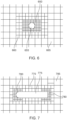
- coarse voxels that interact with fine voxels or VR facets are exploded into a collection of fine voxels (step 1312).
- the states of a coarse voxel that will transmit particles to a fine voxel within a single coarse time step are exploded.
- the appropriate states of a coarse voxel that is not intersected by a facet are exploded into eight fine voxels oriented like the microblock of FIG. 4 .
- the appropriate states of coarse voxel that is intersected by one or more facets are exploded into a collection of complete and/or partial fine voxels corresponding to the portion of the coarse voxel that is not intersected by any facets.
- the particle densities N i (x) for a coarse voxel and the fine voxels resulting from the explosion thereof are equal, but the fine voxels may have fractional factors P f that differ from the fractional factor of the coarse voxel and from the fractional factors of the other fine voxels.
- step 1314 surface dynamics are performed for the fine facets F ⁇ IF and F ⁇ F (step 1314), and for the black facets F ⁇ ICb (step 1316). Dynamics are performed using the procedure illustrated in FIG. 11 and discussed above.
- particles are moved between fine voxels (step 1318) including actual fine voxels and fine voxels resulting from the explosion of coarse voxels. Once the particles have been moved, particles are scattered from the fine facets F ⁇ IF and F ⁇ F to the fine voxels (step 1320).
- Particles are also scattered from the black facets F ⁇ ICb to the fine voxels (including the fine voxels that result from exploding a coarse voxel) (step 1322). Particles are scattered to a fine voxel if the voxel would have received particles at that time absent the presence of a surface.
- particles are scattered to a voxel N(x) when the voxel is an actual fine voxel (as opposed to a fine voxel resulting from the explosion of a coarse voxel), when a voxel N(x + c i ) that is one velocity unit beyond the voxel N(x) is an actual fine voxel, or when the voxel N(x + c i ) that is one velocity unit beyond the voxel N(x) is a fine voxel resulting from the explosion of a coarse voxel.
- the first fine time step is completed by performing fluid dynamics on the fine voxels (step 1324).
- the voxels for which fluid dynamics are performed do not include the fine voxels that result from exploding a coarse voxel (step 1312).
- the procedure 1300 implements similar steps during the second fine time step. Initially, particles are moved between surfaces in a second surface-to-surface advection stage (step 1326). Particles are advected from black facets to red facets, from black facets to fine facets, from fine facets to red facets, and from fine facets to fine facets.
- particles are gathered from the voxels in a second gather stage (steps 1328-1330). Particles are gathered for red facets F ⁇ IRr from fine voxels using fine parallelepipeds (step 1328). Particles also are gathered for fine facets F ⁇ F and F ⁇ IF from fine voxels using fine parallelepipeds (step 1330).
- step 1332 surface dynamics are performed for the fine facets F ⁇ IF and F ⁇ F (step 1332), for the coarse facets F ⁇ C (step 1134), and for the red facets F ⁇ ICr (step 1336) as discussed above.
- particles are moved between voxels using fine resolution (step 1338) so that particles are moved to and from fine voxels and fine voxels representative of coarse voxels.
- Particles are then moved between voxels using coarse resolution (step 1340) so that particles are moved to and from coarse voxels.
- particles are scattered from the facets to the voxels while the fine voxels that represent coarse voxels (i.e., the fine voxels resulting from exploding coarse voxels) are coalesced into coarse voxels (step 1342).
- particles are scattered from coarse facets to coarse voxels using coarse parallelepipeds, from fine facets to fine voxels using fine parallelepipeds, from red facets to fine or coarse voxels using fine parallelepipeds, and from black facets to coarse voxels using the differences between coarse parallelepipeds and find parallelepipeds.
- fluid dynamics are performed for the fine voxels and the coarse voxels (step 1344).
- ⁇ is the PM resistivity.
- porosity between 0 and 1
- the interface effect may be significant for certain types of applications, such as flow acoustics.
- FIG. 14 illustrates a fluid F flowing toward an interface surface 1401 of a porous medium PM with porosity ⁇ .
- the fraction of the surface that is penetrable and into which the fluid may flow is only ⁇ .
- the fraction of the surface that is blocked by the PM solid structure is 1- ⁇ .
- a fluid is represented by fluid particles, i.e., fluid fluxes, such as mass momentum energy fluxes, and particle distributions
- the ⁇ fraction of particles is allowed to move into the PM during particle advection, and the 1- ⁇ fraction of particles is constrained by the PM solid wall boundary condition (BC).
- the fluid particles may include particle distributions or fluxes of hydrodynamic and thermodynamic properties such as mass fluxes, momentum fluxes, and energy fluxes.
- the fluid particles, or elements may include properties such as mass, density, momentum, pressure, velocity, temperature, and energy.
- the elements may be associated with any fluid, flow, or thermodynamic related quantity although not exhaustively identified herein.
- a frictional wall (botince-back or turbulent wall) BC or a frictionless wall BC can be applied.
- the fraction of particles allowed to move into the PM affects the mass and momentum conditions in the direction normal to the interface.
- a frictionless wall or a frictional wall BC can be applied (as is true for a "typical" wall boundary).
- a frictionless wall BC maintains the surface tangential fluid velocity on the wall by not modifying the flux of tangential momentum at the interface.
- a frictional wall BC does alter the tangential momentum flux to achieve, for example, a no-slip wall boundary condition, or a turbulent wall model.
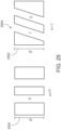
- the PM interface X can be described by so-called double-sided surface elements (i.e., surfels), as shown in FIG. 15 .
- a set of paired surfels S form a double-layered surface having an inner surface A and outer surface B.
- the inner surface A interacts with the PM and the outer surface B interacts with fluid domain Fd.
- each inner surfel has the exact same shape and size as its paired outer surfel, and each inner surfel is only in touch with the paired outer surfel.
- the standard surfel gather and scatter scheme is performed on each side of the surface A, B, and with the condition that the ⁇ f fraction of incoming particles from the fluid side F pass through to the PM side while all of the incoming particles ⁇ PM from the PM side pass through to the fluid side F.
- Advantages of this approach include simplified handling of the complex PM interface, exact satisfaction of conservation laws, and easy realization of specified fluid boundary conditions on PM interface.
- a fluid flow region FF may be adjacent to a region PM occupied by a PM material with sound absorbing properties, with a PM interface X providing the interface between the fluid flow region FF and the region PM, and a wall interface Y providing the interface between the region PM and a wall W.
- the fluid flow region FF and the region PM can be, in effect, treated as two separate simulation spaces having different properties (e.g., in the region PM, an increased impedance may be used to account for the presence of the PM impedance), with movements ⁇ and 1- ⁇ between the two simulation spaces FF, PM being governed by the properties of the PM interface, as discussed above.
- CFD Computational Fluid Dynamics
- CAA Computational AeroAcoustics
- a time-explicit CFD/CAA solution method based on the Lattice Boltzmann Method (LBM), which has evolved over the last two decades as an alternative numerical method to traditional CFD, may be used.
- LBM Lattice Boltzmann Method
- the resulting compressible and unsteady solution method may be used for predicting a variety of complex flow physics, such as aeroacoustics and pure acoustics problems.
- a porous media model is used to represent the flow resistivity of various components, such as air filters, radiators, heat exchangers, evaporators, and other components, which are encountered in simulating flow, such as through HVAC systems, vehicle engine compartments, and other applications.
- ⁇ 0 is the density of air
- c 0 the sound speed in air
- the LBM-PM model approach correctly captures both flow and acoustic effects, even for a material that has a significant flow resistance effect but a negligible effect on acoustics.
- HVAC heating, ventilation, and air conditioning
- the HVAC system is complex, consisting of a blower and mixing unit coupled to many ducts through which air is transported to various locations, including faces and feet of front and rear passengers, as well as windshield and sideglass defrost.
- the blower must supply sufficient pressure head to achieve desired air flow rates for each thermal comfort setting. Noise is generated due to the blower rotation, and by the turbulent air flow in the mixing unit, through the twists and turns of the ducts, and exiting the registers (ventilation outlets).
- the duct and mixing unit flow noise sources are generated mainly by flow separations and vortices resulting from the detailed geometric features, and are also acoustically propagated through the system. Noise due to the flow exiting the registers depends on the fine details of the grill and its orientation, and the resulting outlet jets which mix with the ambient air and may impact surfaces, such as the windshield 2308 (e.g., for defrost). Therefore, the requirements for numerical flow-acoustic predictions may be accomplished using the exemplary modeling, as detailed above, whereby the interior cabin 2302 may be considered a fluid of a first volume and the static components and surfaces within the interior cabin 2302 may be considered a second volume occupied by a porous medium. By implementing the exemplary modeling, complex geometries may be investigated to provide predictions of the fan and flow induced noise sources, and their acoustic propagation all the way through the system to the locations of the passengers at the interior cabin 2302 of the vehicle 2300.
- the PM model accounts for tortuosity of the medium. For example, it may be desirable to model the acoustic behavior of sound waves as the waves propagate through a porous medium. Modelling this behavior can be difficult to when the exact geometry of the porous medium is unknown. (e.g. when modeling the propagation of acoustic waves through, for example, foam padding).
- the following example illustrates the time scaling, a 1D (3D extension is straightforward) small perturbation assumption for acoustic analysis.
- u is the fluid velocity
- p static pressure
- ⁇ 0 is characteristic density
- ⁇ is the PM resistance
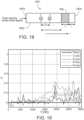
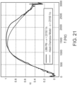
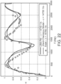
- FIG. 26 shows the effects of tortuosity on the curve of absorption coefficient versus frequency for the NASA ceramic liner porous media.
- the liner is composed of straight micro circular tubes with porosity of 0.57 and tortuosity of 1.0.
- the first line 2602 and second line 2604 are PowerFLOW (registry 17836) results with the tortuosity equal to 2.0 and 1.0 respectively.
- the frequency corresponding to the first line 2602 curve is scaled by the factor of 1 / 2 , which agrees with the tortuosity of 2 for this case and is in full agreement with the time scaling given by Eq. (46).
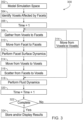
- FIG. 27 is a flow chart of an example process 2700 for processing data representing acoustic properties of a porous medium modeled in accordance with tortuosity.
- the process can be performed by a data processing apparatus, such as a computer system.
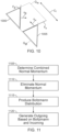
- the process 2700 includes generating 2702 a model of acoustic behavior of a fluid filled porous media including an effect of tortuosity, with the model comprising a time variable indicative of a sound speed of the fluid.
- the process 2700 includes rescaling 2704 the time variable of the model based on the sound speed in a fluid in the porous medium. Rescaling the time variable can include adjusting the amount of time represented by one simulation time step.
- the time may be rescaled based on a streamline length of the porous medium and a thickness of the porous medium being simulated. As the time is rescaled, the temperature and/or pressure within the model may also be rescaled.
- the term "data processing apparatus” encompasses all kinds of apparatus, devices, and machines for processing data, including by way of example: a programmable processor, a computer, a system on a chip, or multiple ones, or combinations, of the foregoing.
- the apparatus can include special purpose logic circuitry (e.g., an FPGA (field programmable gate array) or an ASIC (application specific integrated circuit)).
- the apparatus can also include, in addition to hardware, code that creates an execution environment for the computer program in question (e.g., code that constitutes processor firmware, a protocol stack, a database management system, an operating system, a cross-platform runtime environment, a virtual machine, or a combination of one or more of them).
- the apparatus and execution environment can realize various different computing model infrastructures, such as web services, distributed computing and grid computing infrastructures.
- a computer program (also known as a program, software, software application, script, or code) can be written in any form of programming language, including compiled or interpreted languages, declarative or procedural languages, and it can be deployed in any form, including as a stand-alone program or as a module, component, subroutine, object, or other unit suitable for use in a computing environment.
- a computer program may, but need not, correspond to a file in a file system.
- a program can be stored in a portion of a file that holds other programs or data (e.g., one or more scripts stored in a markup language document), in a single file dedicated to the program in question, or in multiple coordinated files (e.g., files that store one or more modules, sub programs, or portions of code).
- a computer program can be deployed to be executed on one computer or on multiple computers that are located at one site or distributed across multiple sites and interconnected by a communication network.
- the processes and logic flows described in this specification can be performed by one or more programmable processors executing one or more computer programs to perform actions by operating on input data and generating output.
- the processes and logic flows can also be performed by, and apparatus can also be implemented as, special purpose logic circuitry (e.g., an FPGA (field programmable gate array) or an ASIC (application specific integrated circuit)).
- special purpose logic circuitry e.g., an FPGA (field programmable gate array) or an ASIC (application specific integrated circuit)
- processors suitable for the execution of a computer program include, by way of example, both general and special purpose microprocessors, and any one or more processors of any kind of digital computer.
- a processor will receive instructions and data from a read only memory or a random access memory or both.
- the essential elements of a computer are a processor for performing actions in accordance with instructions and one or more memory devices for storing instructions and data.
- a computer will also include, or be operatively coupled to receive data from or transfer data to, or both, one or more mass storage devices for storing data (e.g., magnetic, magneto optical disks, or optical disks), however, a computer need not have such devices.
- a computer can be embedded in another device (e.g., a mobile telephone, a personal digital assistant (PDA), a mobile audio or video player, a game console, a Global Positioning System (GPS) receiver, or a portable storage device (e.g., a universal serial bus (USB) flash drive)).
- Devices suitable for storing computer program instructions and data include all forms of non-volatile memory, media and memory devices, including by way of example, semiconductor memory devices (e.g., EPROM, EEPROM, and flash memory devices), magnetic disks (e.g., internal hard disks or removable disks), magneto optical disks, and CD ROM and DVD-ROM disks.
- the processor and the memory can be supplemented by, or incorporated in, special purpose logic circuitry.
- a computer having a display device (e.g., a CRT (cathode ray tube) or LCD (liquid crystal display) monitor) for displaying information to the user and a keyboard and a pointing device (e.g., a mouse or a trackball) by which the user can provide input to the computer.
- a display device e.g., a CRT (cathode ray tube) or LCD (liquid crystal display) monitor
- a keyboard and a pointing device e.g., a mouse or a trackball
- Other kinds of devices can be used to provide for interaction with a user as well; for example, feedback provided to the user can be any form of sensory feedback (e.g., visual feedback, auditory feedback, or tactile feedback) and input from the user can be received in any form, including acoustic, speech, or tactile input.
- a computer can interact with a user by sending documents to and receiving documents from a device that is used by the user (for example, by sending web pages to a web
- Embodiments of the subject matter described in this specification can be implemented in a computing system that includes a back end component (e.g., as a data server), or that includes a middleware component (e.g., an application server), or that includes a front end component (e.g., a user computer having a graphical user interface or a Web browser through which a user can interact with an implementation of the subject matter described in this specification), or any combination of one or more such back end, middleware, or front end components.
- the components of the system can be interconnected by any form or medium of digital data communication (e.g., a communication network).
- Examples of communication networks include a local area network (“LAN”) and a wide area network (“WAN”), an inter-network (e.g., the Internet), and peer-to-peer networks (e.g., ad hoc peer-to-peer networks).
- LAN local area network
- WAN wide area network
- inter-network e.g., the Internet
- peer-to-peer networks e.g., ad hoc peer-to-peer networks.
- the computing system can include users and servers.
- a user and server are generally remote from each other and typically interact through a communication network. The relationship of user and server arises by virtue of computer programs running on the respective computers and having a user-server relationship to each other.
- a server transmits data (e.g., an HTML page) to a user device (e.g., for purposes of displaying data to and receiving user input from a user interacting with the user device).
- Data generated at the user device e.g., a result of the user interaction
Landscapes
- Engineering & Computer Science (AREA)
- Physics & Mathematics (AREA)
- Theoretical Computer Science (AREA)
- General Physics & Mathematics (AREA)
- General Engineering & Computer Science (AREA)
- Computer Hardware Design (AREA)
- Evolutionary Computation (AREA)
- Geometry (AREA)
- Management, Administration, Business Operations System, And Electronic Commerce (AREA)
- Data Mining & Analysis (AREA)
- Computational Mathematics (AREA)
- Mathematical Analysis (AREA)
- Mathematical Physics (AREA)
- Pure & Applied Mathematics (AREA)
- Mathematical Optimization (AREA)
- Operations Research (AREA)
- Evolutionary Biology (AREA)
- Bioinformatics & Computational Biology (AREA)
- Probability & Statistics with Applications (AREA)
- Life Sciences & Earth Sciences (AREA)
- Algebra (AREA)
- Bioinformatics & Cheminformatics (AREA)
- Databases & Information Systems (AREA)
- Software Systems (AREA)
Applications Claiming Priority (2)
| Application Number | Priority Date | Filing Date | Title |
|---|---|---|---|
| US14/994,943 US10262087B2 (en) | 2016-01-13 | 2016-01-13 | Data processing method for including the effect of the tortuosity on the acoustic behavior of a fluid in a porous medium |
| PCT/US2017/012079 WO2017123435A1 (en) | 2016-01-13 | 2017-01-04 | A data processing method for including the effect of the tortuosity on the acoustic behavior of a fluid in a porous medium |
Publications (4)
| Publication Number | Publication Date |
|---|---|
| EP3403204A1 EP3403204A1 (en) | 2018-11-21 |
| EP3403204A4 EP3403204A4 (en) | 2019-09-11 |
| EP3403204C0 EP3403204C0 (en) | 2024-08-21 |
| EP3403204B1 true EP3403204B1 (en) | 2024-08-21 |
Family
ID=59275672
Family Applications (1)
| Application Number | Title | Priority Date | Filing Date |
|---|---|---|---|
| EP17738742.0A Active EP3403204B1 (en) | 2016-01-13 | 2017-01-04 | A data processing method for including the effect of the tortuosity on the acoustic behavior of a fluid in a porous medium |
Country Status (4)
| Country | Link |
|---|---|
| US (2) | US10262087B2 (enExample) |
| EP (1) | EP3403204B1 (enExample) |
| JP (1) | JP6728366B2 (enExample) |
| WO (1) | WO2017123435A1 (enExample) |
Families Citing this family (13)
| Publication number | Priority date | Publication date | Assignee | Title |
|---|---|---|---|---|
| JP6292203B2 (ja) * | 2015-09-25 | 2018-03-14 | トヨタ自動車株式会社 | 音検出装置 |
| US11042674B2 (en) * | 2017-10-10 | 2021-06-22 | Dassault Systemes Simulia Corp. | Acoustic effects of a mesh on a fluid flow |
| CN109509220B (zh) * | 2018-11-06 | 2021-12-14 | 北京理工大学 | 一种模拟多孔介质固相转换器内部流体流动的方法 |
| CN110321619B (zh) * | 2019-06-26 | 2020-09-15 | 深圳技术大学 | 基于声音数据的参数化定制模型生成方法 |
| CN110427730B (zh) * | 2019-08-22 | 2020-12-29 | 西北工业大学 | 一种齿轮箱全局等效统计能量分析建模方法 |
| KR102200443B1 (ko) * | 2019-12-13 | 2021-01-08 | 이에이트 주식회사 | Lbm 기반의 유체 해석 시뮬레이션 장치, 방법 및 컴퓨터 프로그램 |
| CN111241734A (zh) * | 2020-01-09 | 2020-06-05 | 上海索辰信息科技有限公司 | 针对活塞式发动机的振动噪声数值模拟方法 |
| CN111709646B (zh) * | 2020-06-17 | 2024-02-09 | 九江学院 | 空气污染暴露风险评价方法及系统 |
| US11847391B2 (en) * | 2020-06-29 | 2023-12-19 | Dassault Systemes Simulia Corp. | Computer system for simulating physical processes using surface algorithm |
| CN112149226B (zh) * | 2020-09-15 | 2023-10-31 | 青岛大学 | 一种基于局部无网格基本解法的车内噪声预测方法 |
| CN113868907A (zh) * | 2021-09-23 | 2021-12-31 | 山东汽车制造有限公司 | 一种空调除霜系统的有限元分析设计方法 |
| CN115438551B (zh) * | 2022-10-10 | 2023-12-08 | 北京理工大学 | 一种计算发动机燃烧室隔热效能的cfd-fem联合仿真方法 |
| CN116306279B (zh) * | 2023-03-15 | 2024-06-07 | 重庆交通大学 | 一种水动力自由面lb模拟方法、系统及存储介质 |
Family Cites Families (8)
| Publication number | Priority date | Publication date | Assignee | Title |
|---|---|---|---|---|
| US7841982B2 (en) | 1995-06-22 | 2010-11-30 | Techniscan, Inc. | Apparatus and method for imaging objects with wavefields |
| US6256600B1 (en) * | 1997-05-19 | 2001-07-03 | 3M Innovative Properties Company | Prediction and optimization method for homogeneous porous material and accoustical systems |
| ITMI20010078A1 (it) | 2001-01-17 | 2002-07-17 | Aermacchi S P A | Pannello acustico a struttura composita migliorato |
| US20110010137A1 (en) | 2009-07-08 | 2011-01-13 | Livermore Software Technology Corporation | Numerical simulation of airflow within porous materials |
| US9037440B2 (en) * | 2011-11-09 | 2015-05-19 | Exa Corporation | Computer simulation of fluid flow and acoustic behavior |
| BRPI1105355B1 (pt) * | 2011-12-20 | 2018-12-04 | Univ Federal De Santa Catarina Ufsc | processo de fabricação de um corpo poroso, por metalurgia do pó e composição metalúrgica de materiais particulados |
| CA2904008C (en) | 2013-03-15 | 2020-10-27 | Schlumberger Canada Limited | Methods of characterizing earth formations using physiochemical model |
| EP2997518A4 (en) | 2013-05-16 | 2017-05-17 | EXA Corporation | Mass exchange model for relative permeability simulation |
-
2016
- 2016-01-13 US US14/994,943 patent/US10262087B2/en active Active
-
2017
- 2017-01-04 WO PCT/US2017/012079 patent/WO2017123435A1/en not_active Ceased
- 2017-01-04 EP EP17738742.0A patent/EP3403204B1/en active Active
- 2017-01-04 JP JP2018536751A patent/JP6728366B2/ja active Active
-
2019
- 2019-03-12 US US16/299,460 patent/US10831952B2/en active Active
Also Published As
| Publication number | Publication date |
|---|---|
| WO2017123435A1 (en) | 2017-07-20 |
| US10262087B2 (en) | 2019-04-16 |
| US10831952B2 (en) | 2020-11-10 |
| EP3403204A4 (en) | 2019-09-11 |
| EP3403204C0 (en) | 2024-08-21 |
| JP6728366B2 (ja) | 2020-07-22 |
| US20170199950A1 (en) | 2017-07-13 |
| US20190266300A1 (en) | 2019-08-29 |
| EP3403204A1 (en) | 2018-11-21 |
| JP2019507418A (ja) | 2019-03-14 |
Similar Documents
| Publication | Publication Date | Title |
|---|---|---|
| US10831952B2 (en) | Data processing method for including the effect of the tortuosity on the acoustic behavior of a fluid in a porous medium | |
| US9646119B2 (en) | Computer simulation of fluid flow and acoustic behavior | |
| EP3695333B1 (en) | Acoustic effects of a mesh on a fluid flow | |
| US11118449B2 (en) | Mass exchange model for relative permeability simulation | |
| US10360324B2 (en) | Computer simulation of physical processes | |
| US9542506B2 (en) | Computer simulation of physical processes including modeling of laminar-to-turbulent transition | |
| EP3525120A1 (en) | Lattice boltzmann collision operators enforcing isotropy and galilean invariance | |
| US20200394277A1 (en) | Computer simulation of physical fluids on irregular spatial grids stabilized for explicit numerical diffusion problems | |
| JP7740897B2 (ja) | コンピュータ支援設計定義のジオメトリにおけるメッシュ空洞空間特定および自動シード検出 | |
| JP2021072123A (ja) | スカラ輸送についてのガリレイ不変を強制する格子ボルツマンベースのスカラ輸送を使用して物理的プロセスをシミュレートするためのコンピュータシステム | |
| Tautz et al. | Source formulations and boundary treatments for Lighthill’s analogy applied to incompressible flows | |
| US20200285709A1 (en) | Turbulent Boundary Layer Modeling via Incorporation of Pressure Gradient Directional Effect | |
| Fares | Numerical Investigation of Noise Generation by Automotive Cooling Fans | |
| Xu | Flow/acoustic interactions in porous media under a turbulent wind environment |
Legal Events
| Date | Code | Title | Description |
|---|---|---|---|
| STAA | Information on the status of an ep patent application or granted ep patent |
Free format text: STATUS: THE INTERNATIONAL PUBLICATION HAS BEEN MADE |
|
| PUAI | Public reference made under article 153(3) epc to a published international application that has entered the european phase |
Free format text: ORIGINAL CODE: 0009012 |
|
| STAA | Information on the status of an ep patent application or granted ep patent |
Free format text: STATUS: REQUEST FOR EXAMINATION WAS MADE |
|
| 17P | Request for examination filed |
Effective date: 20180813 |
|
| AK | Designated contracting states |
Kind code of ref document: A1 Designated state(s): AL AT BE BG CH CY CZ DE DK EE ES FI FR GB GR HR HU IE IS IT LI LT LU LV MC MK MT NL NO PL PT RO RS SE SI SK SM TR |
|
| AX | Request for extension of the european patent |
Extension state: BA ME |
|
| DAV | Request for validation of the european patent (deleted) | ||
| DAX | Request for extension of the european patent (deleted) | ||
| RAP1 | Party data changed (applicant data changed or rights of an application transferred) |
Owner name: DASSAULT SYSTEMES SIMULIA CORP. |
|
| A4 | Supplementary search report drawn up and despatched |
Effective date: 20190812 |
|
| RIC1 | Information provided on ipc code assigned before grant |
Ipc: G06F 17/50 20060101AFI20190806BHEP |
|
| STAA | Information on the status of an ep patent application or granted ep patent |
Free format text: STATUS: EXAMINATION IS IN PROGRESS |
|
| 17Q | First examination report despatched |
Effective date: 20210510 |
|
| REG | Reference to a national code |
Ref legal event code: R079 Ipc: G06F0030230000 Ref country code: DE Ref legal event code: R079 Ref document number: 602017084251 Country of ref document: DE Free format text: PREVIOUS MAIN CLASS: G06F0017500000 Ipc: G06F0030230000 |
|
| GRAP | Despatch of communication of intention to grant a patent |
Free format text: ORIGINAL CODE: EPIDOSNIGR1 |
|
| STAA | Information on the status of an ep patent application or granted ep patent |
Free format text: STATUS: GRANT OF PATENT IS INTENDED |
|
| RIC1 | Information provided on ipc code assigned before grant |
Ipc: G06F 30/23 20200101AFI20240227BHEP |
|
| INTG | Intention to grant announced |
Effective date: 20240314 |
|
| RAP1 | Party data changed (applicant data changed or rights of an application transferred) |
Owner name: DASSAULT SYSTEMES AMERICAS CORP. |
|
| GRAS | Grant fee paid |
Free format text: ORIGINAL CODE: EPIDOSNIGR3 |
|
| GRAA | (expected) grant |
Free format text: ORIGINAL CODE: 0009210 |
|
| STAA | Information on the status of an ep patent application or granted ep patent |
Free format text: STATUS: THE PATENT HAS BEEN GRANTED |
|
| AK | Designated contracting states |
Kind code of ref document: B1 Designated state(s): AL AT BE BG CH CY CZ DE DK EE ES FI FR GB GR HR HU IE IS IT LI LT LU LV MC MK MT NL NO PL PT RO RS SE SI SK SM TR |
|
| REG | Reference to a national code |
Ref country code: GB Ref legal event code: FG4D |
|
| REG | Reference to a national code |
Ref country code: CH Ref legal event code: EP |
|
| REG | Reference to a national code |
Ref country code: IE Ref legal event code: FG4D |
|
| REG | Reference to a national code |
Ref country code: DE Ref legal event code: R096 Ref document number: 602017084251 Country of ref document: DE |
|
| U01 | Request for unitary effect filed |
Effective date: 20240916 |
|
| U07 | Unitary effect registered |
Designated state(s): AT BE BG DE DK EE FI FR IT LT LU LV MT NL PT RO SE SI Effective date: 20241007 |
|
| U20 | Renewal fee for the european patent with unitary effect paid |
Year of fee payment: 9 Effective date: 20241205 |
|
| PG25 | Lapsed in a contracting state [announced via postgrant information from national office to epo] |
Ref country code: NO Free format text: LAPSE BECAUSE OF FAILURE TO SUBMIT A TRANSLATION OF THE DESCRIPTION OR TO PAY THE FEE WITHIN THE PRESCRIBED TIME-LIMIT Effective date: 20241121 |
|
| PG25 | Lapsed in a contracting state [announced via postgrant information from national office to epo] |
Ref country code: PL Free format text: LAPSE BECAUSE OF FAILURE TO SUBMIT A TRANSLATION OF THE DESCRIPTION OR TO PAY THE FEE WITHIN THE PRESCRIBED TIME-LIMIT Effective date: 20240821 Ref country code: GR Free format text: LAPSE BECAUSE OF FAILURE TO SUBMIT A TRANSLATION OF THE DESCRIPTION OR TO PAY THE FEE WITHIN THE PRESCRIBED TIME-LIMIT Effective date: 20241122 |
|
| PGFP | Annual fee paid to national office [announced via postgrant information from national office to epo] |
Ref country code: GB Payment date: 20241128 Year of fee payment: 9 |
|
| PG25 | Lapsed in a contracting state [announced via postgrant information from national office to epo] |
Ref country code: IS Free format text: LAPSE BECAUSE OF FAILURE TO SUBMIT A TRANSLATION OF THE DESCRIPTION OR TO PAY THE FEE WITHIN THE PRESCRIBED TIME-LIMIT Effective date: 20241221 |
|
| PG25 | Lapsed in a contracting state [announced via postgrant information from national office to epo] |
Ref country code: HR Free format text: LAPSE BECAUSE OF FAILURE TO SUBMIT A TRANSLATION OF THE DESCRIPTION OR TO PAY THE FEE WITHIN THE PRESCRIBED TIME-LIMIT Effective date: 20240821 |
|
| PG25 | Lapsed in a contracting state [announced via postgrant information from national office to epo] |
Ref country code: RS Free format text: LAPSE BECAUSE OF FAILURE TO SUBMIT A TRANSLATION OF THE DESCRIPTION OR TO PAY THE FEE WITHIN THE PRESCRIBED TIME-LIMIT Effective date: 20241121 Ref country code: ES Free format text: LAPSE BECAUSE OF FAILURE TO SUBMIT A TRANSLATION OF THE DESCRIPTION OR TO PAY THE FEE WITHIN THE PRESCRIBED TIME-LIMIT Effective date: 20240821 |
|
| PG25 | Lapsed in a contracting state [announced via postgrant information from national office to epo] |
Ref country code: RS Free format text: LAPSE BECAUSE OF FAILURE TO SUBMIT A TRANSLATION OF THE DESCRIPTION OR TO PAY THE FEE WITHIN THE PRESCRIBED TIME-LIMIT Effective date: 20241121 Ref country code: PL Free format text: LAPSE BECAUSE OF FAILURE TO SUBMIT A TRANSLATION OF THE DESCRIPTION OR TO PAY THE FEE WITHIN THE PRESCRIBED TIME-LIMIT Effective date: 20240821 Ref country code: NO Free format text: LAPSE BECAUSE OF FAILURE TO SUBMIT A TRANSLATION OF THE DESCRIPTION OR TO PAY THE FEE WITHIN THE PRESCRIBED TIME-LIMIT Effective date: 20241121 Ref country code: IS Free format text: LAPSE BECAUSE OF FAILURE TO SUBMIT A TRANSLATION OF THE DESCRIPTION OR TO PAY THE FEE WITHIN THE PRESCRIBED TIME-LIMIT Effective date: 20241221 Ref country code: HR Free format text: LAPSE BECAUSE OF FAILURE TO SUBMIT A TRANSLATION OF THE DESCRIPTION OR TO PAY THE FEE WITHIN THE PRESCRIBED TIME-LIMIT Effective date: 20240821 Ref country code: GR Free format text: LAPSE BECAUSE OF FAILURE TO SUBMIT A TRANSLATION OF THE DESCRIPTION OR TO PAY THE FEE WITHIN THE PRESCRIBED TIME-LIMIT Effective date: 20241122 Ref country code: ES Free format text: LAPSE BECAUSE OF FAILURE TO SUBMIT A TRANSLATION OF THE DESCRIPTION OR TO PAY THE FEE WITHIN THE PRESCRIBED TIME-LIMIT Effective date: 20240821 |
|
| PG25 | Lapsed in a contracting state [announced via postgrant information from national office to epo] |
Ref country code: SM Free format text: LAPSE BECAUSE OF FAILURE TO SUBMIT A TRANSLATION OF THE DESCRIPTION OR TO PAY THE FEE WITHIN THE PRESCRIBED TIME-LIMIT Effective date: 20240821 |
|
| PG25 | Lapsed in a contracting state [announced via postgrant information from national office to epo] |
Ref country code: CZ Free format text: LAPSE BECAUSE OF FAILURE TO SUBMIT A TRANSLATION OF THE DESCRIPTION OR TO PAY THE FEE WITHIN THE PRESCRIBED TIME-LIMIT Effective date: 20240821 |
|
| PG25 | Lapsed in a contracting state [announced via postgrant information from national office to epo] |
Ref country code: SK Free format text: LAPSE BECAUSE OF FAILURE TO SUBMIT A TRANSLATION OF THE DESCRIPTION OR TO PAY THE FEE WITHIN THE PRESCRIBED TIME-LIMIT Effective date: 20240821 |
|
| PLBE | No opposition filed within time limit |
Free format text: ORIGINAL CODE: 0009261 |
|
| STAA | Information on the status of an ep patent application or granted ep patent |
Free format text: STATUS: NO OPPOSITION FILED WITHIN TIME LIMIT |
|
| 26N | No opposition filed |
Effective date: 20250522 |
|
| REG | Reference to a national code |
Ref country code: CH Ref legal event code: PL |
|
| PG25 | Lapsed in a contracting state [announced via postgrant information from national office to epo] |
Ref country code: MC Free format text: LAPSE BECAUSE OF FAILURE TO SUBMIT A TRANSLATION OF THE DESCRIPTION OR TO PAY THE FEE WITHIN THE PRESCRIBED TIME-LIMIT Effective date: 20240821 |
|
| PG25 | Lapsed in a contracting state [announced via postgrant information from national office to epo] |
Ref country code: CH Free format text: LAPSE BECAUSE OF NON-PAYMENT OF DUE FEES Effective date: 20250131 |