EP3028071B1 - Method and device for the generation and application of anisotropic elastic parameters in horizontal transverse isotropic (hti) media - Google Patents
Method and device for the generation and application of anisotropic elastic parameters in horizontal transverse isotropic (hti) media Download PDFInfo
- Publication number
- EP3028071B1 EP3028071B1 EP14742555.7A EP14742555A EP3028071B1 EP 3028071 B1 EP3028071 B1 EP 3028071B1 EP 14742555 A EP14742555 A EP 14742555A EP 3028071 B1 EP3028071 B1 EP 3028071B1
- Authority
- EP
- European Patent Office
- Prior art keywords
- anisotropic
- seismic
- parameter data
- anisotropy
- isotropic
- Prior art date
- Legal status (The legal status is an assumption and is not a legal conclusion. Google has not performed a legal analysis and makes no representation as to the accuracy of the status listed.)
- Active
Links
- 238000000034 method Methods 0.000 title claims description 128
- 238000004458 analytical method Methods 0.000 claims description 34
- 230000010354 integration Effects 0.000 claims description 8
- 230000001131 transforming effect Effects 0.000 claims description 7
- 238000012545 processing Methods 0.000 claims description 6
- 239000004215 Carbon black (E152) Substances 0.000 claims description 4
- 229930195733 hydrocarbon Natural products 0.000 claims description 4
- 150000002430 hydrocarbons Chemical class 0.000 claims description 4
- 238000003672 processing method Methods 0.000 claims 4
- 230000004044 response Effects 0.000 description 12
- 230000000694 effects Effects 0.000 description 10
- 230000014509 gene expression Effects 0.000 description 8
- 238000001615 p wave Methods 0.000 description 7
- 239000011435 rock Substances 0.000 description 7
- 230000008569 process Effects 0.000 description 5
- 238000004590 computer program Methods 0.000 description 4
- 230000001419 dependent effect Effects 0.000 description 4
- 238000009795 derivation Methods 0.000 description 4
- 238000002310 reflectometry Methods 0.000 description 4
- 238000005259 measurement Methods 0.000 description 3
- 239000004576 sand Substances 0.000 description 3
- 230000008901 benefit Effects 0.000 description 2
- 238000007405 data analysis Methods 0.000 description 2
- 238000002474 experimental method Methods 0.000 description 2
- 238000010348 incorporation Methods 0.000 description 2
- 238000011835 investigation Methods 0.000 description 2
- 230000000155 isotopic effect Effects 0.000 description 2
- 238000010606 normalization Methods 0.000 description 2
- 238000000926 separation method Methods 0.000 description 2
- 238000013517 stratification Methods 0.000 description 2
- 240000004760 Pimpinella anisum Species 0.000 description 1
- 229920000535 Tan II Polymers 0.000 description 1
- 230000003466 anti-cipated effect Effects 0.000 description 1
- 238000005452 bending Methods 0.000 description 1
- 230000005540 biological transmission Effects 0.000 description 1
- 230000008859 change Effects 0.000 description 1
- 238000006243 chemical reaction Methods 0.000 description 1
- 238000004891 communication Methods 0.000 description 1
- 230000000052 comparative effect Effects 0.000 description 1
- 230000010485 coping Effects 0.000 description 1
- 230000001066 destructive effect Effects 0.000 description 1
- 238000001514 detection method Methods 0.000 description 1
- 238000011161 development Methods 0.000 description 1
- 238000010586 diagram Methods 0.000 description 1
- 238000009826 distribution Methods 0.000 description 1
- 239000012530 fluid Substances 0.000 description 1
- 230000005484 gravity Effects 0.000 description 1
- 238000003475 lamination Methods 0.000 description 1
- 239000000203 mixture Substances 0.000 description 1
- 238000012986 modification Methods 0.000 description 1
- 230000004048 modification Effects 0.000 description 1
- 238000005457 optimization Methods 0.000 description 1
- 238000007781 pre-processing Methods 0.000 description 1
- 230000008707 rearrangement Effects 0.000 description 1
- 230000000717 retained effect Effects 0.000 description 1
- 239000013049 sediment Substances 0.000 description 1
- 239000007787 solid Substances 0.000 description 1
- 238000003860 storage Methods 0.000 description 1
- 238000006467 substitution reaction Methods 0.000 description 1
Images


Classifications
-
- G—PHYSICS
- G01—MEASURING; TESTING
- G01V—GEOPHYSICS; GRAVITATIONAL MEASUREMENTS; DETECTING MASSES OR OBJECTS; TAGS
- G01V1/00—Seismology; Seismic or acoustic prospecting or detecting
- G01V1/28—Processing seismic data, e.g. analysis, for interpretation, for correction
- G01V1/282—Application of seismic models, synthetic seismograms
-
- G—PHYSICS
- G01—MEASURING; TESTING
- G01V—GEOPHYSICS; GRAVITATIONAL MEASUREMENTS; DETECTING MASSES OR OBJECTS; TAGS
- G01V1/00—Seismology; Seismic or acoustic prospecting or detecting
- G01V1/28—Processing seismic data, e.g. analysis, for interpretation, for correction
- G01V1/30—Analysis
-
- G—PHYSICS
- G06—COMPUTING; CALCULATING OR COUNTING
- G06F—ELECTRIC DIGITAL DATA PROCESSING
- G06F17/00—Digital computing or data processing equipment or methods, specially adapted for specific functions
- G06F17/10—Complex mathematical operations
-
- G—PHYSICS
- G01—MEASURING; TESTING
- G01V—GEOPHYSICS; GRAVITATIONAL MEASUREMENTS; DETECTING MASSES OR OBJECTS; TAGS
- G01V2210/00—Details of seismic processing or analysis
- G01V2210/60—Analysis
- G01V2210/62—Physical property of subsurface
- G01V2210/626—Physical property of subsurface with anisotropy
Definitions
- Embodiments of the subject matter disclosed herein generally relate to methods and devices for seismic data modeling and the interpretation and estimating of earth parameters from seismic data and, more particularly, to methods and devices for incorporating and accounting for the effects of anisotropy in seismic applications associated with HTI media.
- Seismic data acquisition involves the generation of seismic waves in the earth using an appropriate source or sources and the recording of the response of the earth to the source waves. Seismic data is routinely acquired to obtain information about subsurface structure, stratigraphy, lithology and fluids contained in the earth's the earth's rocks.
- the seismic response is in part generated by the reflection of seismic waves in the subsurface where there are changes in those earth properties that impact seismic wave propagation.
- the process that describes how source signals propagate and how the response is formed is termed seismic wave propagation.
- Modeling is used to gain understanding of seismic wave propagation and to help analyze seismic signals.
- a model of earth properties is posed and a seismic wave propagation modeling algorithm is used to synthesize seismic responses.
- Models of earth properties are often specified in terms of physical parameters.
- An example is the group of modeling methods that today are widely used to study changes in seismic reflection amplitudes with changing angle of incidence of a plane wave reflecting from a flat interface. See, e.g., Castagna, J. P. and Backus, M. M., Eds., "Offset-dependent reflectivity - Theory and practice of AVO analysis", 1993, Investigations in Geophysics Series No. 8, Society of Exploration Geophysicists, chapter I .
- each half-space can be described with just three earth parameters, e.g., p-wave velocity, s-wave velocity and density.
- earth parameters e.g., p-wave velocity, s-wave velocity and density.
- triplets of parameters may be used, e.g., p-wave impedance, s-wave impedance and density.
- elastic parameters e.g., modeling methods start from other earth parameters, and the transforms to elastic parameters are included as part of the modeling method.
- Seismic modeling is often referred to as forward modeling.
- the reverse process of forward modeling is called inverse modeling or inversion.
- the goal of inversion is to estimate earth parameters given the measured seismic responses.
- Many inversion methods are available and known to those skilled in the art. They all have in common that they are based on some forward model of seismic wave propagation. Some of these methods make use of certain input elastic parameter data, e.g., in the form of low frequency trend information or statistical distributions. Other inversion methods do not use elastic parameters upon input, and use some calibration of seismic amplitudes, performed in a pre-processing step or as part of an algorithm.
- Dependent on the seismic data acquisition geometries, estimates of earth rock properties obtained from any of these inversion methods are generally provided as a series of 2D sections or 3D volumes of elastic parameters.
- Inversion is generally followed by a step of analysis and interpretation of the inversion results. Available borehole log measurements are used to support the analysis and interpretation.
- anisotropic seismic data The earth parameters that describe anisotropy are referred to as anisotropy parameters.
- anisotropy parameters To improve the accuracy of seismic modeling, wavelet estimation, inversion, and the analysis and interpretation of inversion results and seismic data in case of anisotropic seismic data requires that anisotropy is accounted for. Examples of methods to handle anisotropy are described by Rüger, A., 2002, “Reflection Coefficients and Azimuthal AVO Analysis in Anisotropic Media", Geophysical Monograph Series No.
- U.S. Patent No. 6,901,333 issued on May 31, 2005, to Van Riel and Debeye , describes techniques for generating and applying anisotropic elastic parameters which address some of these problems for so-called vertically transverse isotropic (VTI) media which possesses polar anisotropy characteristics.
- VTI vertically transverse isotropic
- HTI horizontally transverse isotropic
- US 2010/0312534 describes a method for modeling anisotropic elastic properties of a subsurface region comprising mixed fractured rocks and other geological bodies.
- P-waves and fast and slow S-waves logs are obtained, and an anisotropic rock physics model of the subsurface region is developed.
- P- and fast and slow S-waves logs at the well direction are calculated using a rock physics model capable of handling fractures and other geological factors. Calculated values are compared to measured values in an iterative model updating process.
- a method according to claim 1 is provided.
- a system according to claim 10 is provided.
- inventions described below include, for example, methods to and systems which incorporate and account for the effects of anisotropy in seismic applications associated with horizontally transverse isotropic (HTI) media, i.e., subsurface layers being imaged which possess azimuthal anisotropy characteristics.
- HTI horizontally transverse isotropic
- embodiments described herein provide a method for transforming earth elastic and anisotropy parameters associated with HTI media into new earth parameters and the use of such anisotropic parameters in such seismic data processing applications or techniques including, but not limited to, for example, seismic modeling, wavelet estimation, inversion, the analysis and interpretation of inversion results, and the analysis and interpretation of seismic data.
- Figure 1 depicts a land seismic exploration system 70 for transmitting and receiving seismic waves intended for seismic exploration in a land environment.
- At least one purpose of system 70 is to determine the absence, or presence of hydrocarbon deposits 44, or at least the probability of the absence or presence of hydrocarbon deposits 44, which are shown in Figure 1 as being located in first sediment layer 16.
- System 70 comprises a source consisting of a vibrator 71, located on first vehicle/truck 73a, operable to generate a seismic signal (transmitted waves), a plurality of receivers 72 (e.g., geophones) for receiving seismic signals and converting them into electrical signals, and seismic data acquisition system 200 (that can be located in, for example, vehicle/truck 73b) for recording the electrical signals generated by receivers 72.
- Source 71, receivers 72, and data acquisition system 200 can be positioned on the surface of ground 75, and all interconnected by one or more cables 12.
- Figure 1 further depicts a single vibrator 71 as the source of transmitted acoustic waves, but it should be understood by those skilled in the art that the source can actually be composed of one or more vibrators 71.
- vehicle 73b can communicate with vehicle 73a via antenna 240a, 240b, respectively, wirelessly.
- Antenna 240c can facilitate communications between receivers 72 and second vehicle 73b and/or first vehicle 73a.
- Vibrator 71 is operated during acquisition so as to generate a seismic signal.
- This signal propagates firstly on the surface of ground 75, in the form of surface waves 74, and secondly in the subsoil, in the form of transmitted ground waves 76 that generate reflected waves 78 when they reach an interface 77 between two geological layers, e.g., first and second layers 16,18, respectively.
- Each receiver 72 receives both surface wave 74 and reflected wave 78 and converts them into an electrical signal in which are superimposed the component corresponding to reflected wave 78 and the component that corresponds to surface wave 74, the latter of which is undesirable and should be filtered out as much as is practically possible.
- Figure 1 depicts a particular land seismic system
- the embodiments described hereto are not limited in their application to seismic data acquired using this type of land seismic system nor are they limited to usage with land seismic systems as a genre, e.g., they can also be used with seismic data acquired using marine seismic systems. More specifically, it is anticipated that seismic data associated with HTI media having azimuthal anisotropy will likely be collected by wide azimuth (WAZ) seismic acquisition systems.
- WAZ wide azimuth
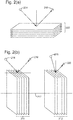
- FIG. 2(a) depicts a VTI anisotropic medium having a plurality of horizontally stratified layers 202, relative to a source 204 and receiver 206 that are used to image the medium.
- VTI media like that shown in Figure 2(a) is typically found where gravity is the dominant factor in the stratification of the layers in the medium to shale, and is otherwise known as media which has polar anisotropy.
- this VTI type of media is that which is analyzed, and whose anisotropy is modeled, in the above U.S. Patent No. 6,901,333 .
- FIG. 2(b) wherein HTI anisotropic mediums 210 and 212 are illustrated.
- the left side of Figure 2(b) illustrates the case with vertically stratified media 210 relative to a source-receiver pair 214, 216 which is oriented in a direction of the principle anisotropy axis 217.
- the right side of Figure 2(b) illustrates another HTI anisotropic medium 212 wherein a source-receiver pair 218, 220 is oriented in a direction perpendicular to the direction of the principle anisotropy axis 217.
- HTI media is typically associated with cracks, fractures and stress and can be found where regional stress is the dominant stratification factor and is otherwise known as media which have azimuthal anisotropy.
- the following embodiments describe techniques for modeling anisotropy parameters associated with media such as that described above with respect to Figure 2(b) .
- AVO Amplitude Versus Offset
- AVO data is converted to other domains, for example to angles for Amplitude Versus Angle (AVA) analysis and interpretation.
- AVA Amplitude Versus Angle
- AVO methods For purposes of the description herein, and in keeping with industry practice, all methods that make use of seismic amplitude changes and in keeping with industry practice, all methods that make use of seismic amplitude changes originating from the measurement of seismic data holding data records with different source-receiver separation are collectively referred to herein as AVO methods.
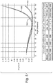
- Figure 3 illustrates, for the example of azimuthal anisotropy, the effect that anisotropy can have on seismic reflection coefficient amplitudes.
- Figure 3 shows the modeled amplitude response of a plane wave incident on a horizontal interface between two layers with and without incorporating HTI anisotropy. The seismic reflection amplitudes are shown as a function of angle (in degrees).
- the solid curve 300 (anis) shows the analytic (exact) reflection coefficient response for a plane wave reflecting from a single, horizontal interface for the case of azimuthal anisotropy and incident and reflected pressure wave.
- the dashed curve 302 (iso) shows the exact solution for the isotropic reflection coefficients.
- the elastic and anisotropy parameters of the layer above and the layer below the interface are specified in the table of Figure 3 , where Vp is the pressure wave velocity in m/s, Vs is the shear wave velocity in m/s, Rho is the density in kg/m3 and eps, del and gam are the Thomsen anisotropy parameters e, ⁇ and ⁇ respectively.
- the properties in the layer above are for an anisotropic shale and those for the layer below are for a water-charged sand that is assumed isotropic.
- the example clearly shows the effect that anisotropy can have on the seismic amplitudes.
- One of the objectives of these embodiments is to define a new class of earth parameters derived from the anisotropy parameters and the elastic parameters, termed anisotropic elastic parameters, for azimuthal anisotropy, such that the effects of azimuthal anisotropy can be modeled to an acceptable level of accuracy when using these parameters in the isotropic modeling of anisotropic seismic data.
- R p ⁇ R 0 + R 2 sin 2 ⁇ + R 4 sin 2 ⁇ tan 2 ⁇ providing the three reflectivity terms for vertical transverse isotropic (VTI) media:
- R 0 1 2 ⁇ Z p Z ⁇ p
- R 0 1 2 ⁇ Z p Z ⁇ p
- the next step is to derive the desired anisotropic elastic parameters, which are denoted by a prime (') accent.
- a close approximation can be obtained by approximating the contrast terms of the anisotropy parameters with new parameters that can be expressed as relative contrasts.
- ⁇ r ⁇ + 1 ⁇ ⁇ ⁇
- the validity of the approximation is verified by calculating the relative contrast of ⁇ r . Taking into account ⁇ ⁇ 1 we see that: ⁇ ⁇ r ⁇ ⁇ r ⁇ ⁇ ⁇ ⁇ The same holds true for ⁇ and ⁇ . When multiple layers are considered, the average can be taken over the set of layers.
- Vs ′ ⁇ r 0.5 / ⁇ r cos 2 ⁇ ⁇ ⁇ ⁇ r / ⁇ r 4 K + 1 / 8 K cos 4 ⁇ ⁇ ⁇ Vs for HTI media.
- This has the advantage that the anisotropic elastic parameters are scaled such that when ⁇ , ⁇ and ⁇ equal 0, they are equal to the input elastic parameters. In comparative data analysis, this nicely emphasizes zones with anisotropy.
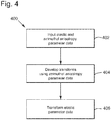
- FIG 4 is a flow chart illustrating the process of one embodiment 400 for deriving azimuthal anisotropic elastic parameters.
- Step 402 represents obtaining the earth elastic parameter data and the azimuthal anisotropy parameter data for an object or imaged area (layer) of interest to use as inputs to the foregoing equations, i.e., data including values for Input V p , V s , ⁇ , ⁇ , ⁇ , y, ⁇ , ⁇ .
- the anisotropy information can be obtained at step 402 by, for example, seismic data processing, where offset and azimuth dependent time shifts are indicative of changes in the propagation velocity. Additionally, at the position of the borehole, one can perform additional seismic experiments to specifically recover HTI and VTI parameters. Such experiments are known as walk-away and walk-around VSP (Vertical Seismic Profiling).
- VSP Vertical Seismic Profiling
- step 404 the transforms are developed, e.g., as shown in Equations 3a', 3b' and 3c', and in step 406 the developed transforms are applied to generate the azimuthal anisotropic elastic parameters, e.g., values for V p ', V s ' and ⁇ ' or I p ', I s ' and ⁇ ' as described above.
- step 406 includes transforming the earth elastic parameter data based on the azimuthal anisotropy parameter data to obtain anisotropic elastic parameter data.
- the output of step 406, i.e., the azimuthal anisotropic elastic parameter data may be applied to at least one of the following methods: isotropic seismic modeling method, an isotropic seismic analysis and interpretation method, an isotropic seismic wavelet estimation method, an isotropic seismic inversion method, or an isotropic method for analysis and interpretation of inversion results.
- the method 400 may also include the step of substituting the azimuthal anisotropic elastic parameter data for isotopic elastic parameters during isotopic seismic modeling method to synthesize anisotropic seismic data. Additionally, the synthesized anisotropic seismic data may be used in an isotropic seismic analysis and interpretation method for analysis and interpretation of anisotropic seismic data. Accordingly, the azimuthal anisotropic elastic parameter data may be substituted for the isotropic elastic parameters in any of the above-mentioned methods.
- Another embodiment is directed to a method for approximating anisotropic seismic modeling by applying isotropic seismic modeling.
- the method includes an initial step of inputting earth elastic parameter data and earth anisotropy parameter data for an area of interest.
- the earth elastic parameter data is transformed to obtain anisotropic elastic parameter data based on the earth anisotropy parameter data.
- Isotropic seismic modeling is then applied on the transformed anisotropic elastic parameter data.
- the resulting modeled anisotropic seismic data is an approximation of seismic data obtained by a corresponding anisotropic seismic modeling.
- the processed anisotropic seismic data is then output.
- the method may further include a step of substituting the anisotropic elastic parameter data for isotropic elastic parameter data to synthesize the anisotropic seismic data.
- the synthesized anisotropic seismic data may be used in an isotropic analysis and interpretation method for analysis and interpretation of the anisotropic seismic data.
- the area of interest may be imaged by acquisition of borehole data, wide azimuth (WAZ) data, three-dimension (3-D) earth models, or four-dimensional (4-D) earth models.
- This step of transforming may further include applying appropriate transform functions that convert the earth elastic parameter data and earth anisotropy parameter data to the anisotropic elastic parameter data.
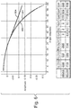
- Figure 5 and Figure 6 illustrate modeling results for two different sets of rock property data, that exhibit relatively strong anisotropy contrasts.
- Figure 5 illustrates the effect, using the same model as for Figure 3 , of using the 3-term approximation for the Zoeppritz equations described above, wherein the curve 500 the anisotropic response and curve 502 shows the isotropic response.
- the dotted curve 504 shows the result of isotropic modeling with the anisotropic elastic parameters specified in the table, where Vpae, Vsae and Rhoae are the anisotropic elastic pressure wave velocity, shear wave velocity and density, respectively, calculated from the transform expressions (3) and using the normalization equation (4).
- FIG. 6 illustrates the same results as in Figure 5 , but for another case.
- the properties in the layer above are for isotropic brine-charged sand and in the layer below are for anisotropic shale.
- curve 600 shows the anisotropic response
- curve 602 shows the isotropic response
- curve 604 shows the response with isotropic modeling with anisotropic elastic parameters.
- the results illustrate that isotropic modeling with the anisotropic elastic parameters closely approximates anisotropic modeling.
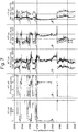
- Figure 7 shows panels with borehole log data to demonstrate the effect of transforming elastic parameters to anisotropic elastic parameters for the case of azimuthal anisotropy and incident and reflecting pressure waves.
- Figure 7 illustrates a suite of borehole logs with pressure ( V p ) and shear wave velocity ( V s ) and density (Rho) elastic parameters, the corresponding anisotropic elastic parameters for azimuthal anisotropy and incident and reflecting pressure waves, the shale volume log (Vshale) and logs of ⁇ r and ⁇ r .
- the normalization of equation (4) has been applied to achieve that the anisotropic elastic parameters are equal to the elastic parameters in the pure sand sections (where the shale volume is zero), for example, between Top Unit II and Top Unit I.
- the above derivation is based on the 3-term approximations to the exact isotropic and exact anisotropic modeling solutions for the plane wave, single horizontal interface model. In practice this may not be the desirable model as different situations in regards to the generation of anisotropic elastic parameters can occur, for example, to handle the following: azimuthal anisotropy for p-wave data; different types of anisotropy for shear and converted wave seismic data; use of the exact equations rather than the 3-term approximation; and use of more complex modeling methods.
- constants x, y and z will generally differ for each of the elastic parameters, for each type of anisotropy and for each wave type (pressure, shear and converted wave). It is also noted that the ⁇ , ⁇ and ⁇ averages are part of the formula. When multiple layers are considered, it can be advantageous to also consider these averages as parameters.
- transform functions are obtained that have parameters that control the transform.
- appropriate values for these transform parameters can be obtained analytically.
- an iterative procedure can also be readily followed to obtain the appropriate values for the transform parameters. This results in further important benefits such as: the exact modeling methods rather than the 3-term approximations can be used as reference for the case of the simple single flat interface model, or more complex modeling methods can be applied; and other transform functions with other functional forms and with other transform parameters than equation (5) can be applied to evaluate if a better approximation can be obtained.
- steps 802 and 804 refer to the input of elastic parameter data and anisotropic parameter data, respectively, which can be obtained as previously described with respect to step 402.
- synthetic azimuthal anisotropic seismic amplitude data is generated using an appropriate azimuthal anisotropic forward modeling method selected on such criteria as the type(s) of anisotropy, wave type(s), model complexity and modeling accuracy. Such data is referred to herein as reference azimuthal anisotropic seismic amplitude data.
- transform functions are developed to transform the earth elastic and anisotropy parameters to anisotropic elastic parameters. It can be assumed that the transform functions have certain parameters (the transform parameters) that may be modified.
- a first set of transform functions may be developed by using some set of initial transform parameters.
- Anisotropic elastic parameters are then generated in step 810 by applying the transforms, e.g., the same or similar as those described above with respect to Equations 3a', 3b' and 3c', to the elastic parameter data.
- isotropic forward modeling is applied with the anisotropic elastic parameters using the isotropic equivalent of the anisotropic forward modeling method used in step 808 to generate anisotropic seismic data.
- This equivalence can generally be achieved by setting the anisotropy parameters to 0 (or constant) in the anisotropic forward modeling method.
- the anisotropic seismic data generated by isotropic modeling with the anisotropic elastic parameters is then compared with the reference anisotropic seismic amplitude data in step 814.
- the comparison is judged. If the comparison from step 816 is not satisfactory, then the parameters of the transform functions are updated in step 818, e.g., the direction of the anisotropy axis and the Thomsen parameters, and the transform functions of step 806 are modified accordingly.
- the decision made in block 816 can, for example, be performed based on an analysis of the HTI data with the WAZ seismic (and synthetic) data which is measuring all of the azimuth directions since the HTI has an isotropic plane that should match the well control and an anisotropic plane orthogonal to the isotropic plane which permits the derivation of the anisotropy, azimuth and the elastic properties. Steps 810-818 are repeated until a satisfactory match is obtained. If the comparison at step 816 is satisfactory, then the set of transform functions is produced in step 820.
- the output of the method of this embodiment is a set of transform functions calibrated for the particular anisotropic forward modeling method selected.
- the generated isotropic elastic parameters as well as the anisotropy parameters may also be output, as may the synthesized anisotropic seismic data.
- the forward modeling method referred to in step 608 may be a method for a two-layer (one interface) earth model, or may be a method for multiple layers, or may be a method for a fully inhomogeneous earth. In the last two cases the modeling and comparison may be carried out over a limited interval of interest.
- the modification in step 818 to a fit-for-purpose level of accuracy may be done automatically using an optimization method, or interactively or in combination.
- the equivalent isotropic forward modeling method may also be used.
- the proposed anisotropic elastic parameter transform expressions achieve the objective that the anisotropic elastic parameters are straightforwardly obtained by a point-by-point transform of the elastic parameters.
- An important implication is that, to handle anisotropy, all available isotropic AVO methods for such applications as seismic modeling, wavelet estimation, the inversion and analysis and interpretation of inversion results, and the analysis and interpretation of seismic amplitude data can continue to be applied simply by replacing the isotropic elastic parameters by the above-defined anisotropic elastic parameters at the appropriate points in these methods.
- the transforms will typically be applied to wide azimuth data with the data points in those data sets representing earth elastic and anisotropy parameters at some spatial location or locations in the earth. It is noted that such representations allow for specification of the vertical location in terms of seismic travel time or in distance or depth.
- anisotropic elastic parameters can also be obtained by integration of the contrast expressions such as equation (1). This may result in improved accuracy, as the conversion of the anisotropy parameters to relative contrasts is not needed. However, this gain may be offset by the practical observation that integration can introduce low frequency drift and requires handling of the integration constant. This may not impact further use of the anisotropic elastic parameters, for example, in certain band-limited seismic modeling and inversion methods where these effects are removed in the method. Hence, these are examples where anisotropic elastic parameters obtained by integration can be effectively used. In fact, in certain of these methods band-limited anisotropic elastic parameters can be used.
- An alternative method is to combine anisotropic elastic parameters obtained by an integration procedure with the anisotropic elastic parameters obtained with the point-by-point transforms. This can be achieved by replacing the low frequency part of the result obtained by the integration procedure with the equivalent part obtained with the point-by-point transforms.
- the transform parameters can be a function of depth or lateral position in the earth.
- the above analytic derivation shows that these transform parameters may be a function of K.
- K varies spatially in the earth.
- the transform parameters are assumed constant when a single interface is used for deriving the transforms or are assumed constant over the study interval of interest. When these transforms are applied over longer intervals or areas, this may lead to a loss to of accuracy. This same issue occurs in conventional seismic AVO analysis, as for example discussed in Fatti, J. L., Smith, G. C., Vail, P. J., Strauss, P. J. and Levitt, P.
- Embodiments are also directed to a device for anisotropic processing of earth elastic parameter data and the application of processed data.
- the device includes a first input means for inputting earth elastic parameter data of an area of interest; a second input means for inputting earth anisotropy parameter data of the area of interest; a transform means for transforming, based on the input earth anisotropy parameter data, the input earth elastic parameter data to obtain anisotropic elastic parameter data; a processor for applying the anisotropic elastic parameter data in at least one of the following methods: 1) an isotropic seismic modeling method; 2) an isotropic seismic analysis and interpretation method; 3) an isotropic seismic wavelet estimation method; 4) an isotropic seismic inversion method; and 5) an isotropic method for the analysis and interpretation of inversion results; and an output means for outputting the processed anisotropic elastic parameter data.
- Another embodiment includes a device for approximating anisotropic seismic modeling by applying isotropic seismic modeling.
- the device includes a first input means for inputting earth elastic parameter data of an area of interest; a second input means for inputting earth anisotropy parameter data of the area of interest; a transform means for transforming, based on the input earth anisotropy parameter data, the input earth elastic parameter data to obtain anisotropic elastic parameter data; a processor for applying the isotropic seismic modeling on the transformed anisotropic elastic parameter data, the resulting modeled anisotropic seismic data being an approximation of the data obtained by a corresponding anisotropic seismic modeling; and an output means for outputting the processed anisotropic seismic data.
- anisotropy parameter data anisotropy parameter data.
- An input/output unit 908 may be connected to the CPU 902 and may be of any conventional type, such as a monitor and keyboard, mouse, touchscreen, printer, and/or voice activated device.
- the computer system 900 runs a computer program to execute instructions for the CPU 902 to perform any of the methods of the embodiments described hereinabove.
- the computer system 900 is simply an example of one suitable computer system for the practice of the embodiments. Such computer systems are well understood by one of ordinary skill in the art.
- the computer program may be stored on a data carrier 910, such as a disk electronically connectable with the CPU 902, so as to allow the computer program when run on a computer to execute any of the methods described hereinabove.
- the disclosed embodiments provide a server node, and methods for generation and application of anisotropic elastic parameters in HTI media. It should be understood that this description is not intended to limit the invention. Further, in the detailed description of the embodiments, numerous specific details are set forth in order to provide a comprehensive understanding of the invention. However, one skilled in the art would understand that various embodiments may be practiced without such specific details.
Description
- The present application is related to, and claims priority from
U.S. Provisional Patent Application No. 61/859,361, filed July 29, 2013 - Embodiments of the subject matter disclosed herein generally relate to methods and devices for seismic data modeling and the interpretation and estimating of earth parameters from seismic data and, more particularly, to methods and devices for incorporating and accounting for the effects of anisotropy in seismic applications associated with HTI media.
- Seismic data acquisition involves the generation of seismic waves in the earth using an appropriate source or sources and the recording of the response of the earth to the source waves. Seismic data is routinely acquired to obtain information about subsurface structure, stratigraphy, lithology and fluids contained in the earth's the earth's rocks. The seismic response is in part generated by the reflection of seismic waves in the subsurface where there are changes in those earth properties that impact seismic wave propagation. The process that describes how source signals propagate and how the response is formed is termed seismic wave propagation.
- Modeling is used to gain understanding of seismic wave propagation and to help analyze seismic signals. In modeling, a model of earth properties is posed and a seismic wave propagation modeling algorithm is used to synthesize seismic responses. Models of earth properties are often specified in terms of physical parameters. An example is the group of modeling methods that today are widely used to study changes in seismic reflection amplitudes with changing angle of incidence of a plane wave reflecting from a flat interface. See, e.g., Castagna, J. P. and Backus, M. M., Eds., "Offset-dependent reflectivity - Theory and practice of AVO analysis", 1993, Investigations in Geophysics Series No. 8, Society of Exploration Geophysicists, chapter I. In this model, the two half-spaces above and below the interface are assumed to be homogeneous and isotropic so that each half-space can be described with just three earth parameters, e.g., p-wave velocity, s-wave velocity and density. In practice alternative triplets of parameters may be used, e.g., p-wave impedance, s-wave impedance and density. These parameters are referred to as elastic parameters. In some cases, modeling methods start from other earth parameters, and the transforms to elastic parameters are included as part of the modeling method.
- Seismic modeling is often referred to as forward modeling. The reverse process of forward modeling is called inverse modeling or inversion. The goal of inversion is to estimate earth parameters given the measured seismic responses. Many inversion methods are available and known to those skilled in the art. They all have in common that they are based on some forward model of seismic wave propagation. Some of these methods make use of certain input elastic parameter data, e.g., in the form of low frequency trend information or statistical distributions. Other inversion methods do not use elastic parameters upon input, and use some calibration of seismic amplitudes, performed in a pre-processing step or as part of an algorithm. Dependent on the seismic data acquisition geometries, estimates of earth rock properties obtained from any of these inversion methods are generally provided as a series of 2D sections or 3D volumes of elastic parameters.
- An important component of modeling and inversion is the seismic wavelet. Many methods are available for wavelet estimation. Inversion is generally followed by a step of analysis and interpretation of the inversion results. Available borehole log measurements are used to support the analysis and interpretation.
- Most of today's routinely applied methods for forward modeling, wavelet estimation, inversion, analysis and interpretation of inversion results, and analysis and interpretation of seismic data have, as a core assumption, that the earth can be locally modeled by a stack of layers, wherein each layer is isotropic, i.e., having a physical parameter or property which has the same value when measured in different directions. Such methods are further referred to herein as "isotropic" methods.
- However, in fact, the earth subsurface is generally anisotropic and acquired seismic data contains the effects of anisotropy. To distinguish such seismic data, it is termed herein "anisotropic seismic data". The earth parameters that describe anisotropy are referred to as anisotropy parameters. To improve the accuracy of seismic modeling, wavelet estimation, inversion, and the analysis and interpretation of inversion results and seismic data in case of anisotropic seismic data requires that anisotropy is accounted for. Examples of methods to handle anisotropy are described by Rüger, A., 2002, "Reflection Coefficients and Azimuthal AVO Analysis in Anisotropic Media", Geophysical Monograph Series No. 10, Society of Exploration Geophysicists; and Thomsen, L., 2002, "Understanding Seismic Anisotropy in Exploration and Exploitation", Distinguished Instructor Series No. 5, Society of Exploration Geophysicists/European Association of Geoscientists and Engineers.
- Incorporation of the anisotropy parameters in these methods makes them mathematically and numerically more complex than the equivalent isotropic methods. Also, methods where seismic modeling is used, such as in wavelet estimation and in certain seismic data analysis and interpretation methods, would need to be extended to incorporate the anisotropy parameters, making them more complex in utilization. Further, from the perspective of inversion, explicit incorporation of anisotropy parameters is even more disadvantageous. Performing inversion for the elastic parameters from amplitude-variation with offset (AVO) seismic data is recognized to be a difficult problem for most seismic data acquisition geometries. For example, including the anisotropy parameters in inversion as parameters that also need to be recovered in the inversion process further increases the number of unknowns and makes the inverse problem more difficult. Addition of more parameters and coping with these difficulties also complicates the analysis and interpretation of inversion results.
-
U.S. Patent No. 6,901,333, issued on May 31, 2005, to Van Riel and Debeye , describes techniques for generating and applying anisotropic elastic parameters which address some of these problems for so-called vertically transverse isotropic (VTI) media which possesses polar anisotropy characteristics. However, not all seismic acquisitions are performed on subsurfaces having VTI media. Instead, some seismic acquisitions are performed on subsurfaces having horizontally transverse isotropic (HTI) media which possess azimuthal anisotropy characteristics.US 2010/0312534 describes a method for modeling anisotropic elastic properties of a subsurface region comprising mixed fractured rocks and other geological bodies. P-waves and fast and slow S-waves logs are obtained, and an anisotropic rock physics model of the subsurface region is developed. P- and fast and slow S-waves logs at the well direction are calculated using a rock physics model capable of handling fractures and other geological factors. Calculated values are compared to measured values in an iterative model updating process. - Accordingly, it would be desirable to provide systems and methods that avoid the afore-described problems and drawbacks, and provide systems and methods to incorporate and generate anisotropy parameters in applications such as seismic modeling, wavelet estimation, inversion and the like, as well as analysis and interpretations of such data, for seismic acquisitions being performed with respect to azimuthally anisotropic (or equivalently, horizontally transverse isotropic (HTI)) media.
- These, and other, aspects associated with processing of seismic data acquired with respect to data acquired via seismic acquisitions being performed with respect to azimuthally anisotropic (or equivalently, horizontally transverse isotropic (HTI)) media are addressed herein.
- According to an embodiment, a method according to claim 1 is provided.
- According to another embodiment, a system according to
claim 10 is provided. - The accompanying drawings, which are incorporated in and constitute a part of the specification, illustrate one or more embodiments and, together with the description, explain these embodiments. In the drawings:
-
Figure 1 illustrates a seismic acquisition system whose acquired data can be processed to compensate for azimuthal anisotropy according to embodiments; -
Figure 2(a) depicts elastic wave reflection from vertically transverse isotropic (VTI) media; -
Figure 2(b) shows elastic wave reflection from horizontally transverse isotropic (HTI) media; -
Figure 3 shows a plot of isotropic and anisotropic seismic reflection coefficient amplitudes as a function of angle; -
Figure 4 is a flowchart of a method according to an embodiment; -
Figure 5 shows a plot of seismic reflection coefficient amplitudes as a function of angle for isotropic elastic parameters, anisotropic elastic parameters and isotropic modeling with the anisotropic elastic parameters for one location; -
Figure 6 shows a plot of seismic reflection coefficient amplitudes as a function of angle for isotropic elastic parameters, anisotropic elastic parameters and isotropic modeling with the anisotropic elastic parameters for another location; -
Figure 7 shows a comparison of elastic parameters and the anisotropic elastic parameters on borehole log data; -
Figure 8 is a flowchart of a method according to another embodiment; and -
Figure 9 shows a block diagram of a computer system which can be used for implementation of embodiments described herein. - The following description of the embodiments refers to the accompanying drawings. The same reference numbers in different drawings identify the same or similar elements. The following detailed description does not limit the invention. Instead, the scope of the invention is defined by the appended claims. Some of the following embodiments are discussed, for simplicity, with regard to the terminology and structure of maximizing the available information associated with parameters variations with a given set of source-receiver pairs by avoiding destructive summation. However, the embodiments to be discussed next are not limited to these configurations, but may be extended to other arrangements as discussed later.
- Reference throughout the specification to "one embodiment" or "an embodiment" means that a particular feature, structure or characteristic described in connection with an embodiment is included in at least one embodiment of the subject matter disclosed. Thus, the appearance of the phrases "in one embodiment" or "in an embodiment" in various places throughout the specification is not necessarily referring to the same embodiment. Further, the particular features, structures or characteristics may be combined in any suitable manner in one or more embodiments.
- The embodiments described below include, for example, methods to and systems which incorporate and account for the effects of anisotropy in seismic applications associated with horizontally transverse isotropic (HTI) media, i.e., subsurface layers being imaged which possess azimuthal anisotropy characteristics. Among other things, embodiments described herein provide a method for transforming earth elastic and anisotropy parameters associated with HTI media into new earth parameters and the use of such anisotropic parameters in such seismic data processing applications or techniques including, but not limited to, for example, seismic modeling, wavelet estimation, inversion, the analysis and interpretation of inversion results, and the analysis and interpretation of seismic data.
- Prior to discussing such embodiments in detail, some context associated with seismic acquisition systems generally, which generate seismic data to which such embodiments can be applied, will first be provided. For example,
Figure 1 depicts a landseismic exploration system 70 for transmitting and receiving seismic waves intended for seismic exploration in a land environment. At least one purpose ofsystem 70 is to determine the absence, or presence ofhydrocarbon deposits 44, or at least the probability of the absence or presence ofhydrocarbon deposits 44, which are shown inFigure 1 as being located infirst sediment layer 16. -
System 70 comprises a source consisting of avibrator 71, located on first vehicle/truck 73a, operable to generate a seismic signal (transmitted waves), a plurality of receivers 72 (e.g., geophones) for receiving seismic signals and converting them into electrical signals, and seismic data acquisition system 200 (that can be located in, for example, vehicle/truck 73b) for recording the electrical signals generated byreceivers 72.Source 71,receivers 72, anddata acquisition system 200, can be positioned on the surface ofground 75, and all interconnected by one ormore cables 12.Figure 1 further depicts asingle vibrator 71 as the source of transmitted acoustic waves, but it should be understood by those skilled in the art that the source can actually be composed of one ormore vibrators 71. Furthermore,vehicle 73b can communicate withvehicle 73a viaantenna Antenna 240c can facilitate communications betweenreceivers 72 andsecond vehicle 73b and/orfirst vehicle 73a. -
Vibrator 71 is operated during acquisition so as to generate a seismic signal. This signal propagates firstly on the surface ofground 75, in the form of surface waves 74, and secondly in the subsoil, in the form of transmittedground waves 76 that generate reflectedwaves 78 when they reach aninterface 77 between two geological layers, e.g., first andsecond layers receiver 72 receives bothsurface wave 74 and reflectedwave 78 and converts them into an electrical signal in which are superimposed the component corresponding to reflectedwave 78 and the component that corresponds to surfacewave 74, the latter of which is undesirable and should be filtered out as much as is practically possible. - Those skilled in the art will appreciate that, although
Figure 1 depicts a particular land seismic system, the embodiments described hereto are not limited in their application to seismic data acquired using this type of land seismic system nor are they limited to usage with land seismic systems as a genre, e.g., they can also be used with seismic data acquired using marine seismic systems. More specifically, it is anticipated that seismic data associated with HTI media having azimuthal anisotropy will likely be collected by wide azimuth (WAZ) seismic acquisition systems. - As mentioned in the Background section, another important contextual consideration for the present discussion is the type of media being imaged by, e.g.,
system 70 described above. Looking toFigures 2(a) and 2(b) examples of the different types of stratified media which can be imaged via seismic acquisition are conceptually illustrated.Figure 2(a) depicts a VTI anisotropic medium having a plurality of horizontally stratifiedlayers 202, relative to asource 204 andreceiver 206 that are used to image the medium. VTI media like that shown inFigure 2(a) is typically found where gravity is the dominant factor in the stratification of the layers in the medium to shale, and is otherwise known as media which has polar anisotropy. As mentioned above, this VTI type of media is that which is analyzed, and whose anisotropy is modeled, in the aboveU.S. Patent No. 6,901,333 . - By way of contrast, consider now
Figure 2(b) wherein HTIanisotropic mediums Figure 2(b) illustrates the case with vertically stratifiedmedia 210 relative to a source-receiver pair principle anisotropy axis 217. The right side ofFigure 2(b) illustrates another HTIanisotropic medium 212 wherein a source-receiver pair principle anisotropy axis 217. It should be noted that HTI media is typically associated with cracks, fractures and stress and can be found where regional stress is the dominant stratification factor and is otherwise known as media which have azimuthal anisotropy. The following embodiments describe techniques for modeling anisotropy parameters associated with media such as that described above with respect toFigure 2(b) . - With this in mind note that, in seismic data, important information about earth elastic and anisotropy parameters is embedded in the change of seismic amplitudes as a function of the separation between sources and receivers. This is referred to as Amplitude Versus Offset (AVO). In many applications AVO data is converted to other domains, for example to angles for Amplitude Versus Angle (AVA) analysis and interpretation. Further, rather than studying the data at the level of records, practitioners often use partial stacks of records. In this way data is reduced and robustness improved, yet the key characteristics of the amplitude changes with offset, angle or other parameter are retained. For purposes of the description herein, and in keeping with industry practice, all methods that make use of seismic amplitude changes and in keeping with industry practice, all methods that make use of seismic amplitude changes originating from the measurement of seismic data holding data records with different source-receiver separation are collectively referred to herein as AVO methods.
- The relationship that links the subsurface parameters to seismic AVO amplitudes is determined by seismic wave propagation modeling. For the most general case this leads to a very complex relationship that can only be solved by numerical wave equation modeling. Most modeling methods in practical use today are based on a simplified wave propagation model.
- An example of a commonly used class of AVO modeling methods, as described by the book edited by Castagna, J. P. and Backus, M. M., entitled "Offset-dependent reflectivity - Theory and practice of AVO analysis", published in the Investigations in Geophysics Series, No. 8, Society of Exploration Geophysicists (1993) hereafter "Castagna", is based on the following simplified seismic wave propagation model: the earth is stratified into isotropic parallel layers; seismic waves propagate as plane waves impinging on each interface at a constant angle; each interface acts as an independent reflector; transmission effects are neglected, other than ray bending; and the calculated plane wave reflection coefficients are based on the assumption of isotropic half spaces above and below the reflector interface.
- Thus, in this specific example, a very simple model of the earth and of wave propagation is assumed. As described by Castagna, even in this example of a simplified seismic wave propagation model, the resulting Zoeppritz equations that describe the AVO relationship are quite complex. Practitioners have therefore turned to approximations of the Zoeppritz equations. In particular, the 3-term Aki-Richards, the 3-term Shuey (which is a rearrangement of the Aki-Richards equation) and 2-term Shuey approximations are widely used. These forward modeling equations or, in more modern methods, the Zoeppritz equations, form the basis for modeling in many seismic AVO inversion methods in use today, as further detailed in the references cited above.
- To further expand the application of AVO methods requires the use of a more practical model than those described above. One important extension is to take into account anisotropy. Anisotropy can seriously affect AVO amplitudes, as demonstrated in
Figure 3. Figure 3 illustrates, for the example of azimuthal anisotropy, the effect that anisotropy can have on seismic reflection coefficient amplitudes. Specifically,Figure 3 shows the modeled amplitude response of a plane wave incident on a horizontal interface between two layers with and without incorporating HTI anisotropy. The seismic reflection amplitudes are shown as a function of angle (in degrees). The solid curve 300 (anis) shows the analytic (exact) reflection coefficient response for a plane wave reflecting from a single, horizontal interface for the case of azimuthal anisotropy and incident and reflected pressure wave. For comparison, the dashed curve 302 (iso) shows the exact solution for the isotropic reflection coefficients. The elastic and anisotropy parameters of the layer above and the layer below the interface are specified in the table ofFigure 3 , where Vp is the pressure wave velocity in m/s, Vs is the shear wave velocity in m/s, Rho is the density in kg/m3 and eps, del and gam are the Thomsen anisotropy parameters e, δ and γ respectively. - In this example the properties in the layer above are for an anisotropic shale and those for the layer below are for a water-charged sand that is assumed isotropic. The example clearly shows the effect that anisotropy can have on the seismic amplitudes.
- One of the objectives of these embodiments is to define a new class of earth parameters derived from the anisotropy parameters and the elastic parameters, termed anisotropic elastic parameters, for azimuthal anisotropy, such that the effects of azimuthal anisotropy can be modeled to an acceptable level of accuracy when using these parameters in the isotropic modeling of anisotropic seismic data.
- This procedure is first illustrated for the case of polar anisotropy for p-wave sources and receivers, extended to include azimuthal anisotropy, and then generalized. The books by Rüger, A., 2002, "Reflection Coefficients and Azimuthal AVO Analysis in Anisotropic Media", Geophysical Monograph Series No. 10, Society of Exploration Geophysicists; and Thomsen, L., 2002, "Understanding Seismic Anisotropy in Exploration and Exploitation", Distinguished Instructor Series No. 5, Society of Exploration Geophysicists/European Association of Geoscientists and Engineers describe how to incorporate anisotropy in AVO modeling. They generalize the above isotropic model to model plane wave reflection in case of anisotropic media. Analogous to the approximation of the Zoeppritz equations by the 3-term Aki-Richards or Shuey equations, they show that for the AVO plane wave reflection coefficients for a flat interface bounded by anisotropic half spaces, a convenient approximation to the AVO relationship can be obtained. The 3-term expression they derive is:


- Rp (θ) being the p-wave reflection coefficient for incident angle θ;
-
Z p ,V p ,V s andG being the average acoustic impedance, p-wave velocity, s-wave velocity and vertical shear modulus (G = ρVs 2) respectively; - ΔZp , ΔVp , ΔVs and ΔG being the acoustic impedance, p-wave velocity, s-wave velocity, and vertical shear modulus contrasts respectively;
- ω being the azimuth of the source-receiver pair in the seismic acquisition;
- φ being the azimuth of the symmetry axis of the HTI media perpendicular to the laminations (see
Figure 2(b) ); and - Δε, Δδ and Δγ being the Thomsen anisotropy parameters contrasts, respectively. It should be noted that by rotating a VTI medium 90° to an HTI medium, by definition the Thomsen parameter Δ∈ becomes - Δ∈. These equations correspond to the analogous equations for the isotropic case when the anisotropy constants are 0.
- The next step is to derive the desired anisotropic elastic parameters, which are denoted by a prime (') accent. Starting with the R 4 term, the anisotropic elastic parameter contrast


Then, substituting into the R 0 term and using the small contrast expansion of the impedance product term gives:

Finally, defining K = (V s /V p )2, substitution into the R 2 gives:

- Back substituting these anisotropic elastic parameters in the isotropic equivalent of equation (1) (anisotropy contrasts set to 0) shows that equation (1) is exactly recovered.
- Thus, expressions are obtained for the anisotropic elastic parameter contrasts. These expressions are composed of a mixture of relative elastic parameter and absolute anisotropy parameter contrasts. In practice, it is advantageous to recover rock properties rather than their relative contrasts. In the current form, to recover the absolute quantities


- A close approximation can be obtained by approximating the contrast terms of the anisotropy parameters with new parameters that can be expressed as relative contrasts. One way this can be achieved is with the following expression:

Taking into account ∈ << 1 we see that:


In the same manner, equation (2b) gives:

Further, equation (2c) gives:

- Analyzing the equations (3a'-3c') certain observations of interest can be noted. For example, P-impedance, being the product of Vp and ρ is invariant for anisotropy. Secondly, for HTI media and azimuthal anisotropy, in the direction orthogonal to the anisotropy axis, where (ω - φ) = 90°, the HTI equations reduce to the isotropic case. Thirdly, for HTI media and azimuthal anisotropy, in the direction parallel to the anisotropy axis, where ω = φ, the HTI equations equate to the VTI equations where Δγ = 0 or γ r = 1. Lastly, for a parameterization in P-impedance (I p), S-impedance (I s) and density (ρ), typical for seismic inversion, the HTI equations (3a'-3c') reduce to:


- It should be noted that for convenience the function:

-
Figure 4 is a flow chart illustrating the process of oneembodiment 400 for deriving azimuthal anisotropic elastic parameters. Step 402 represents obtaining the earth elastic parameter data and the azimuthal anisotropy parameter data for an object or imaged area (layer) of interest to use as inputs to the foregoing equations, i.e., data including values for Input V p, V s, ρ, ε, δ, y, ω, φ. The anisotropy information can be obtained atstep 402 by, for example, seismic data processing, where offset and azimuth dependent time shifts are indicative of changes in the propagation velocity. Additionally, at the position of the borehole, one can perform additional seismic experiments to specifically recover HTI and VTI parameters. Such experiments are known as walk-away and walk-around VSP (Vertical Seismic Profiling). - In
step 404 the transforms are developed, e.g., as shown in Equations 3a', 3b' and 3c', and instep 406 the developed transforms are applied to generate the azimuthal anisotropic elastic parameters, e.g., values for V p', V s' and ρ' or I p', I s' and ρ' as described above. In more detail,step 406 includes transforming the earth elastic parameter data based on the azimuthal anisotropy parameter data to obtain anisotropic elastic parameter data. The output ofstep 406, i.e., the azimuthal anisotropic elastic parameter data, may be applied to at least one of the following methods: isotropic seismic modeling method, an isotropic seismic analysis and interpretation method, an isotropic seismic wavelet estimation method, an isotropic seismic inversion method, or an isotropic method for analysis and interpretation of inversion results. - The
method 400 may also include the step of substituting the azimuthal anisotropic elastic parameter data for isotopic elastic parameters during isotopic seismic modeling method to synthesize anisotropic seismic data. Additionally, the synthesized anisotropic seismic data may be used in an isotropic seismic analysis and interpretation method for analysis and interpretation of anisotropic seismic data. Accordingly, the azimuthal anisotropic elastic parameter data may be substituted for the isotropic elastic parameters in any of the above-mentioned methods. - Another embodiment is directed to a method for approximating anisotropic seismic modeling by applying isotropic seismic modeling. The method includes an initial step of inputting earth elastic parameter data and earth anisotropy parameter data for an area of interest. Next, the earth elastic parameter data is transformed to obtain anisotropic elastic parameter data based on the earth anisotropy parameter data. Isotropic seismic modeling is then applied on the transformed anisotropic elastic parameter data. The resulting modeled anisotropic seismic data is an approximation of seismic data obtained by a corresponding anisotropic seismic modeling. The processed anisotropic seismic data is then output.
- The method may further include a step of substituting the anisotropic elastic parameter data for isotropic elastic parameter data to synthesize the anisotropic seismic data. The synthesized anisotropic seismic data may be used in an isotropic analysis and interpretation method for analysis and interpretation of the anisotropic seismic data. The area of interest may be imaged by acquisition of borehole data, wide azimuth (WAZ) data, three-dimension (3-D) earth models, or four-dimensional (4-D) earth models. This step of transforming may further include applying appropriate transform functions that convert the earth elastic parameter data and earth anisotropy parameter data to the anisotropic elastic parameter data.
-
Figure 5 andFigure 6 illustrate modeling results for two different sets of rock property data, that exhibit relatively strong anisotropy contrasts.Figure 5 illustrates the effect, using the same model as forFigure 3 , of using the 3-term approximation for the Zoeppritz equations described above, wherein thecurve 500 the anisotropic response andcurve 502 shows the isotropic response.. In addition, the dottedcurve 504 shows the result of isotropic modeling with the anisotropic elastic parameters specified in the table, where Vpae, Vsae and Rhoae are the anisotropic elastic pressure wave velocity, shear wave velocity and density, respectively, calculated from the transform expressions (3) and using the normalization equation (4). The results show that isotropic modeling with the anisotropic elastic parameters closely approximates anisotropic modeling.Figure 6 illustrates the same results as inFigure 5 , but for another case. In this example the properties in the layer above are for isotropic brine-charged sand and in the layer below are for anisotropic shale. Thus,curve 600 shows the anisotropic response,curve 602 shows the isotropic response andcurve 604 shows the response with isotropic modeling with anisotropic elastic parameters. Again, the results illustrate that isotropic modeling with the anisotropic elastic parameters closely approximates anisotropic modeling. - Modeling with the above equations clearly supports that, even in these cases, the approximation of anisotropic modeling by using the newly defined anisotropic elastic parameters in isotropic modeling is accurate.
-
Figure 7 shows panels with borehole log data to demonstrate the effect of transforming elastic parameters to anisotropic elastic parameters for the case of azimuthal anisotropy and incident and reflecting pressure waves.Figure 7 illustrates a suite of borehole logs with pressure (Vp ) and shear wave velocity (Vs ) and density (Rho) elastic parameters, the corresponding anisotropic elastic parameters for azimuthal anisotropy and incident and reflecting pressure waves, the shale volume log (Vshale) and logs of ε r and δr . The normalization of equation (4) has been applied to achieve that the anisotropic elastic parameters are equal to the elastic parameters in the pure sand sections (where the shale volume is zero), for example, between Top Unit II and Top Unit I. - The above derivation is based on the 3-term approximations to the exact isotropic and exact anisotropic modeling solutions for the plane wave, single horizontal interface model. In practice this may not be the desirable model as different situations in regards to the generation of anisotropic elastic parameters can occur, for example, to handle the following: azimuthal anisotropy for p-wave data; different types of anisotropy for shear and converted wave seismic data; use of the exact equations rather than the 3-term approximation; and use of more complex modeling methods.
- Rüger, A., 2002, "Reflection Coefficients and Azimuthal AVO Analysis in Anisotropic Media", Geophysical Monograph Series No. 10, Society of Exploration Geophysicists demonstrates that, for the plane wave, horizontal interface model, for different types of anisotropy and wave types (pressure shear and converted) the exact solution can be approximated by 3-term equations similar in form to equation (1). Following the derivation procedure above leads to the conclusion that, when using the 3-term equations, the solutions for each of the anisotropic elastic parameters take the general form:

ε ,δ andγ averages are part of the formula. When multiple layers are considered, it can be advantageous to also consider these averages as parameters. - In this way transform functions are obtained that have parameters that control the transform. In some cases appropriate values for these transform parameters can be obtained analytically. However, in another embodiment, an iterative procedure can also be readily followed to obtain the appropriate values for the transform parameters. This results in further important benefits such as: the exact modeling methods rather than the 3-term approximations can be used as reference for the case of the simple single flat interface model, or more complex modeling methods can be applied; and other transform functions with other functional forms and with other transform parameters than equation (5) can be applied to evaluate if a better approximation can be obtained.
- The steps in such an iterative procedure according to an embodiment are further illustrated in the flow chart of
Figure 8 . Initially, steps 802 and 804 refer to the input of elastic parameter data and anisotropic parameter data, respectively, which can be obtained as previously described with respect to step 402. Instep 808, synthetic azimuthal anisotropic seismic amplitude data is generated using an appropriate azimuthal anisotropic forward modeling method selected on such criteria as the type(s) of anisotropy, wave type(s), model complexity and modeling accuracy. Such data is referred to herein as reference azimuthal anisotropic seismic amplitude data. - In
step 806, transform functions are developed to transform the earth elastic and anisotropy parameters to anisotropic elastic parameters. It can be assumed that the transform functions have certain parameters (the transform parameters) that may be modified. A first set of transform functions may be developed by using some set of initial transform parameters. Anisotropic elastic parameters are then generated instep 810 by applying the transforms, e.g., the same or similar as those described above with respect to Equations 3a', 3b' and 3c', to the elastic parameter data. Next, in step 812, isotropic forward modeling is applied with the anisotropic elastic parameters using the isotropic equivalent of the anisotropic forward modeling method used instep 808 to generate anisotropic seismic data. This equivalence can generally be achieved by setting the anisotropy parameters to 0 (or constant) in the anisotropic forward modeling method. The anisotropic seismic data generated by isotropic modeling with the anisotropic elastic parameters is then compared with the reference anisotropic seismic amplitude data instep 814. Instep 816, the comparison is judged. If the comparison fromstep 816 is not satisfactory, then the parameters of the transform functions are updated instep 818, e.g., the direction of the anisotropy axis and the Thomsen parameters, and the transform functions ofstep 806 are modified accordingly. The decision made inblock 816 can, for example, be performed based on an analysis of the HTI data with the WAZ seismic (and synthetic) data which is measuring all of the azimuth directions since the HTI has an isotropic plane that should match the well control and an anisotropic plane orthogonal to the isotropic plane which permits the derivation of the anisotropy, azimuth and the elastic properties. Steps 810-818 are repeated until a satisfactory match is obtained. If the comparison atstep 816 is satisfactory, then the set of transform functions is produced instep 820. - The output of the method of this embodiment is a set of transform functions calibrated for the particular anisotropic forward modeling method selected. The generated isotropic elastic parameters as well as the anisotropy parameters may also be output, as may the synthesized anisotropic seismic data. The forward modeling method referred to in step 608 may be a method for a two-layer (one interface) earth model, or may be a method for multiple layers, or may be a method for a fully inhomogeneous earth. In the last two cases the modeling and comparison may be carried out over a limited interval of interest. The modification in
step 818 to a fit-for-purpose level of accuracy may be done automatically using an optimization method, or interactively or in combination. Instead of in step 812 using the anisotropic forward modeling method, the equivalent isotropic forward modeling method may also be used. - It is recognized that in the method utilizing an iterative procedure to find satisfactory transform parameters the functional form of the transforms is set in the transform development step. If a satisfactory comparison is not achieved after sufficient iterations, alternative transform functions may be evaluated.
- The proposed anisotropic elastic parameter transform expressions achieve the objective that the anisotropic elastic parameters are straightforwardly obtained by a point-by-point transform of the elastic parameters. An important implication is that, to handle anisotropy, all available isotropic AVO methods for such applications as seismic modeling, wavelet estimation, the inversion and analysis and interpretation of inversion results, and the analysis and interpretation of seismic amplitude data can continue to be applied simply by replacing the isotropic elastic parameters by the above-defined anisotropic elastic parameters at the appropriate points in these methods. Within these methods the transforms will typically be applied to wide azimuth data with the data points in those data sets representing earth elastic and anisotropy parameters at some spatial location or locations in the earth. It is noted that such representations allow for specification of the vertical location in terms of seismic travel time or in distance or depth.
- In the above, a method is derived to obtain anisotropic elastic parameters using point-by-point transforms. This is convenient, but is not a difficult requirement. Anisotropic elastic parameters can also be obtained by integration of the contrast expressions such as equation (1). This may result in improved accuracy, as the conversion of the anisotropy parameters to relative contrasts is not needed. However, this gain may be offset by the practical observation that integration can introduce low frequency drift and requires handling of the integration constant. This may not impact further use of the anisotropic elastic parameters, for example, in certain band-limited seismic modeling and inversion methods where these effects are removed in the method. Hence, these are examples where anisotropic elastic parameters obtained by integration can be effectively used. In fact, in certain of these methods band-limited anisotropic elastic parameters can be used.
- An alternative method is to combine anisotropic elastic parameters obtained by an integration procedure with the anisotropic elastic parameters obtained with the point-by-point transforms. This can be achieved by replacing the low frequency part of the result obtained by the integration procedure with the equivalent part obtained with the point-by-point transforms.
- The transform parameters, such as x, y and z can be a function of depth or lateral position in the earth. For example, the above analytic derivation shows that these transform parameters may be a function of K. It is well known that K varies spatially in the earth. In the proposed method the transform parameters are assumed constant when a single interface is used for deriving the transforms or are assumed constant over the study interval of interest. When these transforms are applied over longer intervals or areas, this may lead to a loss to of accuracy. This same issue occurs in conventional seismic AVO analysis, as for example discussed in Fatti, J. L., Smith, G. C., Vail, P. J., Strauss, P. J. and Levitt, P. R., 1994, "Detection of gas in sandstone reservoirs using AVO analysis: A 3D seismic case history using the Geostack technique", Geophysics, vol. 59, no. 9, pp. 1362-1376. Allowing laterally and vertically varying trends in the variables overcomes this problem, where a trend constitutes a spatially varying variable such that its bandwidth is lower than that of the seismic data. The same method can be used for anisotropic elastic parameters by allowing these parameters to take the form of laterally and vertically varying trends.
- Embodiments are also directed to a device for anisotropic processing of earth elastic parameter data and the application of processed data. The device includes a first input means for inputting earth elastic parameter data of an area of interest; a second input means for inputting earth anisotropy parameter data of the area of interest; a transform means for transforming, based on the input earth anisotropy parameter data, the input earth elastic parameter data to obtain anisotropic elastic parameter data; a processor for applying the anisotropic elastic parameter data in at least one of the following methods: 1) an isotropic seismic modeling method; 2) an isotropic seismic analysis and interpretation method; 3) an isotropic seismic wavelet estimation method; 4) an isotropic seismic inversion method; and 5) an isotropic method for the analysis and interpretation of inversion results; and an output means for outputting the processed anisotropic elastic parameter data.
- Another embodiment includes a device for approximating anisotropic seismic modeling by applying isotropic seismic modeling. The device includes a first input means for inputting earth elastic parameter data of an area of interest; a second input means for inputting earth anisotropy parameter data of the area of interest; a transform means for transforming, based on the input earth anisotropy parameter data, the input earth elastic parameter data to obtain anisotropic elastic parameter data; a processor for applying the isotropic seismic modeling on the transformed anisotropic elastic parameter data, the resulting modeled anisotropic seismic data being an approximation of the data obtained by a corresponding anisotropic seismic modeling; and an output means for outputting the processed anisotropic seismic data.
anisotropy parameter data. An input/output unit 908 may be connected to theCPU 902 and may be of any conventional type, such as a monitor and keyboard, mouse, touchscreen, printer, and/or voice activated device. Thecomputer system 900 runs a computer program to execute instructions for theCPU 902 to perform any of the methods of the embodiments described hereinabove. Thecomputer system 900 is simply an example of one suitable computer system for the practice of the embodiments. Such computer systems are well understood by one of ordinary skill in the art. The computer program may be stored on adata carrier 910, such as a disk electronically connectable with theCPU 902, so as to allow the computer program when run on a computer to execute any of the methods described hereinabove. - The disclosed embodiments provide a server node, and methods for generation and application of anisotropic elastic parameters in HTI media. It should be understood that this description is not intended to limit the invention. Further, in the detailed description of the embodiments, numerous specific details are set forth in order to provide a comprehensive understanding of the invention. However, one skilled in the art would understand that various embodiments may be practiced without such specific details.
- Although the features and elements of the present embodiments are described in the embodiments in particular combinations, each feature or element can be used alone without the other features and elements of the embodiments or in various combinations with or without other features and elements disclosed herein. The methods or flow charts provided in the present application may be implemented art would understand that various embodiments may be practiced without such specific details.
- Although the features and elements of the present embodiments are described in the embodiments in particular combinations, each feature or element can be used alone without the other features and elements of the embodiments or in various combinations with or without other features and elements disclosed herein. The methods or flow charts provided in the present application may be implemented in a computer program, software, or firmware tangibly embodied in a computer-readable storage medium for execution by a general purpose computer or a processor.
- This written description uses examples of the subject matter disclosed to enable any person skilled in the art to practice the same, including making and using any devices or systems and performing any incorporated methods. The patentable scope of the subject matter is defined by the claims, and may include other examples that occur to those skilled in the art. Such other examples are intended to be within the scope of the claims.
Claims (15)
- A method for anisotropic processing of earth elastic parameter data associated with a horizontal transverse isotropy (HTI) anisotropic medium, said medium having vertically stratified layers relative to a source-receiver pair and comprising a principle anisotropy axis, the method comprising:acquiring seismic data for an area of interest that includes a layer of an HTI anisotropic medium having azimuthal anisotropic characteristics, using at least one source and receivers, ;obtaining earth elastic parameter data (802) associated with the area of interest;obtaining earth anisotropy parameter data (804) from said area of interest, using an azimuth of the source-receiver pair in the seismic acquisition and using an azimuth of the principle anisotropy axis of the HTI medium perpendicular to the layers ;developing transform functions (806) that transform the earth elastic and anisotropy parameter data into anisotropic elastic parameter data, based on the obtained earth anisotropy parameter data;applying (810) said transform functions to the earth elastic and anisotropy parameter data to obtain said anisotropic elastic parameter data.applying the anisotropic elastic parameter data in at least one seismic processing method to determine at least the probability of the absence or presence of hydrocarbon deposits.
- The method of claim 1, further comprising: applying the anisotropic elastic parameter data in at least one seismic processing method selected from the group including: i) an isotropic seismic modeling method, ii) an isotropic seismic analysis and interpretation method, iii) an isotropic seismic wavelet estimation method, iv) an isotropic seismic inversion method, and v) an isotropic method for analysis and interpretation of inversion results to produce processed anisotropic elastic parameter data.
- The method of claim 2, further comprising substituting the anisotropic elastic parameter data for isotropic elastic parameter data in the isotropic method for analysis and interpretation of inversion results.
- The method of claim 1, wherein the area of interest is imaged using a wide azimuth seismic acquisition technique to obtain said elastic parameter data and said anisotropic parameter data.
- The method of claim 1, wherein the transform functions are

- The method of claim 1, wherein transforming elastic parameter data to anisotropic elastic parameter data is obtained by integration of anisotropic elastic parameter contrasts.
- The method of claim 1, wherein the anisotropy parameter data are transformed to anisotropy relative contrast parameters such that relative contrasts of the transformed anisotropy parameters approximate the contrasts in the anisotropy parameter data.
- The method of claim 1, further comprising:
applying isotropic seismic modeling on the transformed anisotropic elastic parameter data to produce anisotropic seismic data, the produced anisotropic seismic data being an approximation of seismic data obtained by anisotropic seismic modeling. - The method of claim 8, further comprising substituting the anisotropic elastic parameter data for isotropic elastic parameter data in isotropic seismic modeling to produce the anisotropic seismic data.
- A system for anisotropic processing of earth elastic parameter data associated with a horizontal transverse isotropy (HTI) anisotropic medium, said medium having vertically stratified layers relative to a source-receiver pair and comprising a principle anisotropy axis, the system comprising:at least one source and receivers operated to acquire seismic data for an area of interest that includes a layer of an HTI anisotropic medium having azimuthal anisotropic characteristics,;at least one processor (902) configured to obtain earth elastic parameter data (802) associated with the area of interest, to obtain earth anisotropy parameter data (804) from said area of interest, using an azimuth of the source-receiver pair in the seismic acquisition and using an azimuth of the principle anisotropy axis of the HTI medium perpendicular to the layers, wherein the processor is further configured to develop transform functions (806, 810) that transform the earth elastic and anisotropy parameter data into anisotropic elastic parameter data,based on the obtained earth anisotropy parameter data, and to apply said transform functions to the earth elastic and anisotropy parameter data to obtain the anisotropic elastic parameter data;wherein the at least one processor is further configured to apply the anisotropic elastic parameter data in at least one seismic processing method to determine at least the probability of the absence or presence of hydrocarbon deposits.
- The system of claim 10, wherein the at least one processor is further configured to apply the anisotropic elastic parameter data in at least one seismic processing method selected from the group including: i) an isotropic seismic modeling method, ii) an isotropic seismic analysis and interpretation method, iii) an isotropic seismic wavelet estimation method, iv) an isotropic seismic inversion method, and v) an isotropic method for analysis and interpretation of inversion results to produce processed anisotropic elastic parameter data.
- The system of claim 11, wherein the at least one processor is further configured to substituting the anisotropic elastic parameter data for isotropic elastic parameter data in the isotropic method for analysis and interpretation of inversion results.
- The system of claim 10, wherein the area of interest is imaged using a wide azimuth seismic acquisition technique to obtain said elastic parameter data and said anisotropic parameter data.
- The system of claim 10, wherein the transform functions are

- The system of claim 10, wherein the at least one processor is further configured to apply isotropic seismic modeling on the transformed anisotropic elastic parameter data to produce anisotropic seismic data, the produced anisotropic seismic data being an approximation of seismic data obtained by anisotropic seismic modeling.
Applications Claiming Priority (2)
| Application Number | Priority Date | Filing Date | Title |
|---|---|---|---|
| US201361859361P | 2013-07-29 | 2013-07-29 | |
| PCT/EP2014/066101 WO2015014762A2 (en) | 2013-07-29 | 2014-07-25 | Method and device for the generation and application of anisotropic elastic parameters in horizontal transverse isotropic (hti) media |
Publications (2)
| Publication Number | Publication Date |
|---|---|
| EP3028071A2 EP3028071A2 (en) | 2016-06-08 |
| EP3028071B1 true EP3028071B1 (en) | 2018-07-18 |
Family
ID=51224964
Family Applications (1)
| Application Number | Title | Priority Date | Filing Date |
|---|---|---|---|
| EP14742555.7A Active EP3028071B1 (en) | 2013-07-29 | 2014-07-25 | Method and device for the generation and application of anisotropic elastic parameters in horizontal transverse isotropic (hti) media |
Country Status (5)
| Country | Link |
|---|---|
| US (1) | US20150293245A1 (en) |
| EP (1) | EP3028071B1 (en) |
| CA (1) | CA2920008C (en) |
| MX (1) | MX2016001417A (en) |
| WO (1) | WO2015014762A2 (en) |
Families Citing this family (19)
| Publication number | Priority date | Publication date | Assignee | Title |
|---|---|---|---|---|
| CA2892995A1 (en) * | 2012-05-24 | 2013-11-28 | Exxonmobil Upstream Research Company | System and method for predicting rock strength |
| US20150149089A1 (en) * | 2013-11-27 | 2015-05-28 | Chevron U.S.A. Inc. | Determining reserves of a reservoir |
| CN105068117B (en) * | 2015-08-25 | 2016-06-08 | 中国矿业大学(北京) | For the AVO inversion method of Fractured medium, device and equipment |
| GB2561486B (en) * | 2016-01-15 | 2021-09-01 | Landmark Graphics Corp | Semblance-based anisotropy parameter estimation using isotropic depth-migrated common image gathers |
| US10520621B2 (en) | 2016-11-23 | 2019-12-31 | Cgg Services Sas | Method and apparatus for simultaneous geostatistical inversion of time-lapse seismic data |
| CN106772578B (en) * | 2016-12-07 | 2018-11-09 | 中国矿业大学(北京) | A kind of method and apparatus of synthetic seismogram |
| CN106646597B (en) * | 2016-12-14 | 2018-11-27 | 中国石油天然气集团有限公司 | The Forward Modeling and device based on spring net model |
| US11243318B2 (en) | 2017-01-13 | 2022-02-08 | Cgg Services Sas | Method and apparatus for unambiguously estimating seismic anisotropy parameters |
| CN106908839B (en) * | 2017-05-05 | 2018-09-28 | 中国石油大学(华东) | A kind of seismic wave accurate reflection coefficient analysis method and device |
| CN109270575B (en) * | 2018-11-02 | 2019-11-26 | 河南理工大学 | A kind of attenuation of seismic waves model construction method equivalent based on building seismic response |
| US11828895B2 (en) | 2019-08-05 | 2023-11-28 | Geosoftware C.V. | Methods and devices using effective elastic parameter values for anisotropic media |
| CN112558153B (en) * | 2019-09-25 | 2022-03-29 | 中国石油天然气股份有限公司 | Oil and gas reservoir prediction method and device for two-phase medium |
| CN111460602B (en) * | 2019-12-06 | 2021-01-29 | 西南石油大学 | Transverse isotropic stratum ground stress prediction method based on rock physics modeling |
| CN111551990B (en) * | 2020-04-07 | 2023-05-23 | 西安科技大学 | Acquisition system for HTI type coal seam seismic wave reflection coefficient |
| CN114185092A (en) * | 2020-09-15 | 2022-03-15 | 中国石油化工股份有限公司 | Method and device for evaluating development degree of horizontal seam of reservoir, electronic equipment and medium |
| CN113009572B (en) * | 2021-02-23 | 2022-07-01 | 成都理工大学 | Method for predicting fracture azimuth angle based on transverse wave polarization analysis |
| CN113341455B (en) * | 2021-06-24 | 2024-02-09 | 中国石油大学(北京) | Viscous anisotropic medium seismic wave numerical simulation method, device and equipment |
| CN113933898B (en) * | 2021-09-23 | 2022-07-19 | 中国地质大学(武汉) | Method, device and equipment for identifying anisotropic characteristics of fractured reservoir and storage medium |
| CN115097520A (en) * | 2022-06-09 | 2022-09-23 | 中国人民解放军国防科技大学 | Frequency-dependent anisotropic shear wave splitting algorithm for multiple VSP data |
Family Cites Families (4)
| Publication number | Priority date | Publication date | Assignee | Title |
|---|---|---|---|---|
| US6901333B2 (en) * | 2003-10-27 | 2005-05-31 | Fugro N.V. | Method and device for the generation and application of anisotropic elastic parameters |
| US8120991B2 (en) * | 2006-11-03 | 2012-02-21 | Paradigm Geophysical (Luxembourg) S.A.R.L. | System and method for full azimuth angle domain imaging in reduced dimensional coordinate systems |
| US8184502B2 (en) * | 2008-02-28 | 2012-05-22 | Exxonmobil Upstream Research Company | Rock physics model for simulating seismic response in layered fractured rocks |
| SG184002A1 (en) * | 2010-03-12 | 2012-10-30 | Cggveritas Services Us Inc | Methods and systems for performing azimuthal simultaneous elastic inversion |
-
2014
- 2014-07-25 MX MX2016001417A patent/MX2016001417A/en active IP Right Grant
- 2014-07-25 US US14/432,543 patent/US20150293245A1/en not_active Abandoned
- 2014-07-25 CA CA2920008A patent/CA2920008C/en active Active
- 2014-07-25 WO PCT/EP2014/066101 patent/WO2015014762A2/en active Application Filing
- 2014-07-25 EP EP14742555.7A patent/EP3028071B1/en active Active
Non-Patent Citations (1)
| Title |
|---|
| RÜGER A: "Variation of P-wave reflectivity with offset and azimuth in anisotropic media", GEOPHYSICS, SOCIETY OF EXPLORATION GEOPHYSICISTS, US, vol. 63, no. 3, 1 May 1998 (1998-05-01), pages 935 - 947, XP002326797, ISSN: 0016-8033, DOI: 10.1190/1.1444405 * |
Also Published As
| Publication number | Publication date |
|---|---|
| MX2016001417A (en) | 2016-08-18 |
| US20150293245A1 (en) | 2015-10-15 |
| CA2920008A1 (en) | 2015-02-05 |
| WO2015014762A2 (en) | 2015-02-05 |
| CA2920008C (en) | 2017-06-13 |
| WO2015014762A3 (en) | 2015-04-02 |
| EP3028071A2 (en) | 2016-06-08 |
Similar Documents
| Publication | Publication Date | Title |
|---|---|---|
| EP3028071B1 (en) | Method and device for the generation and application of anisotropic elastic parameters in horizontal transverse isotropic (hti) media | |
| US6901333B2 (en) | Method and device for the generation and application of anisotropic elastic parameters | |
| US8352190B2 (en) | Method for analyzing multiple geophysical data sets | |
| Warner et al. | Anisotropic 3D full-waveform inversion | |
| EP3076205B1 (en) | Method for survey data processing compensating for visco-acoustic effects in tilted transverse isotropy reverse time migration | |
| AU2014273165B2 (en) | High resolution estimation of attenuation from vertical seismic profiles | |
| US7315783B2 (en) | Traveltime calculation in three dimensional transversely isotropic (3D TI) media by the fast marching method | |
| AU2011224165B2 (en) | Methods and systems for performing azimuthal simultaneous elastic inversion | |
| US6826484B2 (en) | 3D prestack time migration method | |
| US7082368B2 (en) | Seismic event correlation and Vp-Vs estimation | |
| EP3358376B1 (en) | Method and apparatus for unambiguously estimating seismic anisotropy parameters | |
| EP2160633B1 (en) | Creating an absorption parameter model | |
| US11493658B2 (en) | Computer-implemented method and system employing nonlinear direct prestack seismic inversion for poisson impedance | |
| US20120095690A1 (en) | Methods and computer-readable medium to implement inversion of angle gathers for rock physics reflectivity attributes | |
| EP3772665A1 (en) | Methods and devices using effective elastic parameter values for anisotropic media | |
| Wang et al. | Multiparameter TTI tomography of P-wave reflection and VSP data | |
| Li et al. | Estimation of porosity, fluid bulk modulus, and stiff-pore volume fraction using a multitrace Bayesian amplitude-variation-with-offset petrophysics inversion in multiporosity reservoirs | |
| Vigh et al. | Elastic full-waveform inversion using OBN data acquisition | |
| US8411529B2 (en) | Walkaway VSP calibrated sonic logs | |
| Landrø et al. | Seismic critical-angle reflectometry: A method to characterize azimuthal anisotropy? | |
| US20220373703A1 (en) | Methods and systems for generating an image of a subterranean formation based on low frequency reconstructed seismic data | |
| Gibson Jr et al. | Modeling and velocity analysis with a wavefront-construction algorithm for anisotropic media | |
| WO2015124960A1 (en) | Systems and methods for improved inversion analysis of seismic data | |
| Grech et al. | Integrating borehole information and surface seismic for velocity anisotropy analysis and depth imaging | |
| US20230305176A1 (en) | Determining properties of a subterranean formation using an acoustic wave equation with a reflectivity parameterization |
Legal Events
| Date | Code | Title | Description |
|---|---|---|---|
| PUAI | Public reference made under article 153(3) epc to a published international application that has entered the european phase |
Free format text: ORIGINAL CODE: 0009012 |
|
| 17P | Request for examination filed |
Effective date: 20160128 |
|
| AK | Designated contracting states |
Kind code of ref document: A2 Designated state(s): AL AT BE BG CH CY CZ DE DK EE ES FI FR GB GR HR HU IE IS IT LI LT LU LV MC MK MT NL NO PL PT RO RS SE SI SK SM TR |
|
| AX | Request for extension of the european patent |
Extension state: BA ME |
|
| 17Q | First examination report despatched |
Effective date: 20160727 |
|
| DAX | Request for extension of the european patent (deleted) | ||
| GRAP | Despatch of communication of intention to grant a patent |
Free format text: ORIGINAL CODE: EPIDOSNIGR1 |
|
| INTG | Intention to grant announced |
Effective date: 20180226 |
|
| RAP1 | Party data changed (applicant data changed or rights of an application transferred) |
Owner name: CGG SERVICES SAS |
|
| GRAS | Grant fee paid |
Free format text: ORIGINAL CODE: EPIDOSNIGR3 |
|
| GRAA | (expected) grant |
Free format text: ORIGINAL CODE: 0009210 |
|
| AK | Designated contracting states |
Kind code of ref document: B1 Designated state(s): AL AT BE BG CH CY CZ DE DK EE ES FI FR GB GR HR HU IE IS IT LI LT LU LV MC MK MT NL NO PL PT RO RS SE SI SK SM TR |
|
| REG | Reference to a national code |
Ref country code: GB Ref legal event code: FG4D |
|
| REG | Reference to a national code |
Ref country code: FR Ref legal event code: PLFP Year of fee payment: 5 |
|
| REG | Reference to a national code |
Ref country code: CH Ref legal event code: EP |
|
| REG | Reference to a national code |
Ref country code: IE Ref legal event code: FG4D |
|
| REG | Reference to a national code |
Ref country code: AT Ref legal event code: REF Ref document number: 1019966 Country of ref document: AT Kind code of ref document: T Effective date: 20180815 |
|
| REG | Reference to a national code |
Ref country code: DE Ref legal event code: R096 Ref document number: 602014028713 Country of ref document: DE |
|
| REG | Reference to a national code |
Ref country code: NL Ref legal event code: FP |
|
| REG | Reference to a national code |
Ref country code: NO Ref legal event code: T2 Effective date: 20180718 |
|
| REG | Reference to a national code |
Ref country code: LT Ref legal event code: MG4D |
|
| REG | Reference to a national code |
Ref country code: AT Ref legal event code: MK05 Ref document number: 1019966 Country of ref document: AT Kind code of ref document: T Effective date: 20180718 |
|
| PG25 | Lapsed in a contracting state [announced via postgrant information from national office to epo] |
Ref country code: PL Free format text: LAPSE BECAUSE OF FAILURE TO SUBMIT A TRANSLATION OF THE DESCRIPTION OR TO PAY THE FEE WITHIN THE PRESCRIBED TIME-LIMIT Effective date: 20180718 Ref country code: LT Free format text: LAPSE BECAUSE OF FAILURE TO SUBMIT A TRANSLATION OF THE DESCRIPTION OR TO PAY THE FEE WITHIN THE PRESCRIBED TIME-LIMIT Effective date: 20180718 Ref country code: RS Free format text: LAPSE BECAUSE OF FAILURE TO SUBMIT A TRANSLATION OF THE DESCRIPTION OR TO PAY THE FEE WITHIN THE PRESCRIBED TIME-LIMIT Effective date: 20180718 Ref country code: SE Free format text: LAPSE BECAUSE OF FAILURE TO SUBMIT A TRANSLATION OF THE DESCRIPTION OR TO PAY THE FEE WITHIN THE PRESCRIBED TIME-LIMIT Effective date: 20180718 Ref country code: GR Free format text: LAPSE BECAUSE OF FAILURE TO SUBMIT A TRANSLATION OF THE DESCRIPTION OR TO PAY THE FEE WITHIN THE PRESCRIBED TIME-LIMIT Effective date: 20181019 Ref country code: BG Free format text: LAPSE BECAUSE OF FAILURE TO SUBMIT A TRANSLATION OF THE DESCRIPTION OR TO PAY THE FEE WITHIN THE PRESCRIBED TIME-LIMIT Effective date: 20181018 Ref country code: AT Free format text: LAPSE BECAUSE OF FAILURE TO SUBMIT A TRANSLATION OF THE DESCRIPTION OR TO PAY THE FEE WITHIN THE PRESCRIBED TIME-LIMIT Effective date: 20180718 Ref country code: IS Free format text: LAPSE BECAUSE OF FAILURE TO SUBMIT A TRANSLATION OF THE DESCRIPTION OR TO PAY THE FEE WITHIN THE PRESCRIBED TIME-LIMIT Effective date: 20181118 Ref country code: FI Free format text: LAPSE BECAUSE OF FAILURE TO SUBMIT A TRANSLATION OF THE DESCRIPTION OR TO PAY THE FEE WITHIN THE PRESCRIBED TIME-LIMIT Effective date: 20180718 |
|
| REG | Reference to a national code |
Ref country code: DE Ref legal event code: R119 Ref document number: 602014028713 Country of ref document: DE |
|
| PG25 | Lapsed in a contracting state [announced via postgrant information from national office to epo] |
Ref country code: HR Free format text: LAPSE BECAUSE OF FAILURE TO SUBMIT A TRANSLATION OF THE DESCRIPTION OR TO PAY THE FEE WITHIN THE PRESCRIBED TIME-LIMIT Effective date: 20180718 Ref country code: LV Free format text: LAPSE BECAUSE OF FAILURE TO SUBMIT A TRANSLATION OF THE DESCRIPTION OR TO PAY THE FEE WITHIN THE PRESCRIBED TIME-LIMIT Effective date: 20180718 Ref country code: AL Free format text: LAPSE BECAUSE OF FAILURE TO SUBMIT A TRANSLATION OF THE DESCRIPTION OR TO PAY THE FEE WITHIN THE PRESCRIBED TIME-LIMIT Effective date: 20180718 |
|
| REG | Reference to a national code |
Ref country code: CH Ref legal event code: PL |
|
| PG25 | Lapsed in a contracting state [announced via postgrant information from national office to epo] |
Ref country code: LU Free format text: LAPSE BECAUSE OF NON-PAYMENT OF DUE FEES Effective date: 20180725 |
|
| REG | Reference to a national code |
Ref country code: BE Ref legal event code: MM Effective date: 20180731 |
|
| REG | Reference to a national code |
Ref country code: IE Ref legal event code: MM4A |
|
| PG25 | Lapsed in a contracting state [announced via postgrant information from national office to epo] |
Ref country code: EE Free format text: LAPSE BECAUSE OF FAILURE TO SUBMIT A TRANSLATION OF THE DESCRIPTION OR TO PAY THE FEE WITHIN THE PRESCRIBED TIME-LIMIT Effective date: 20180718 Ref country code: IT Free format text: LAPSE BECAUSE OF FAILURE TO SUBMIT A TRANSLATION OF THE DESCRIPTION OR TO PAY THE FEE WITHIN THE PRESCRIBED TIME-LIMIT Effective date: 20180718 Ref country code: RO Free format text: LAPSE BECAUSE OF FAILURE TO SUBMIT A TRANSLATION OF THE DESCRIPTION OR TO PAY THE FEE WITHIN THE PRESCRIBED TIME-LIMIT Effective date: 20180718 Ref country code: CH Free format text: LAPSE BECAUSE OF NON-PAYMENT OF DUE FEES Effective date: 20180731 Ref country code: CZ Free format text: LAPSE BECAUSE OF FAILURE TO SUBMIT A TRANSLATION OF THE DESCRIPTION OR TO PAY THE FEE WITHIN THE PRESCRIBED TIME-LIMIT Effective date: 20180718 Ref country code: DE Free format text: LAPSE BECAUSE OF NON-PAYMENT OF DUE FEES Effective date: 20190201 Ref country code: ES Free format text: LAPSE BECAUSE OF FAILURE TO SUBMIT A TRANSLATION OF THE DESCRIPTION OR TO PAY THE FEE WITHIN THE PRESCRIBED TIME-LIMIT Effective date: 20180718 Ref country code: IE Free format text: LAPSE BECAUSE OF NON-PAYMENT OF DUE FEES Effective date: 20180725 Ref country code: LI Free format text: LAPSE BECAUSE OF NON-PAYMENT OF DUE FEES Effective date: 20180731 Ref country code: MC Free format text: LAPSE BECAUSE OF FAILURE TO SUBMIT A TRANSLATION OF THE DESCRIPTION OR TO PAY THE FEE WITHIN THE PRESCRIBED TIME-LIMIT Effective date: 20180718 |
|
| PLBE | No opposition filed within time limit |
Free format text: ORIGINAL CODE: 0009261 |
|
| STAA | Information on the status of an ep patent application or granted ep patent |
Free format text: STATUS: NO OPPOSITION FILED WITHIN TIME LIMIT |
|
| PG25 | Lapsed in a contracting state [announced via postgrant information from national office to epo] |
Ref country code: SK Free format text: LAPSE BECAUSE OF FAILURE TO SUBMIT A TRANSLATION OF THE DESCRIPTION OR TO PAY THE FEE WITHIN THE PRESCRIBED TIME-LIMIT Effective date: 20180718 Ref country code: SM Free format text: LAPSE BECAUSE OF FAILURE TO SUBMIT A TRANSLATION OF THE DESCRIPTION OR TO PAY THE FEE WITHIN THE PRESCRIBED TIME-LIMIT Effective date: 20180718 Ref country code: BE Free format text: LAPSE BECAUSE OF NON-PAYMENT OF DUE FEES Effective date: 20180731 Ref country code: DK Free format text: LAPSE BECAUSE OF FAILURE TO SUBMIT A TRANSLATION OF THE DESCRIPTION OR TO PAY THE FEE WITHIN THE PRESCRIBED TIME-LIMIT Effective date: 20180718 |
|
| 26N | No opposition filed |
Effective date: 20190423 |
|
| PG25 | Lapsed in a contracting state [announced via postgrant information from national office to epo] |
Ref country code: SI Free format text: LAPSE BECAUSE OF FAILURE TO SUBMIT A TRANSLATION OF THE DESCRIPTION OR TO PAY THE FEE WITHIN THE PRESCRIBED TIME-LIMIT Effective date: 20180718 |
|
| PG25 | Lapsed in a contracting state [announced via postgrant information from national office to epo] |
Ref country code: MT Free format text: LAPSE BECAUSE OF NON-PAYMENT OF DUE FEES Effective date: 20180725 |
|
| PG25 | Lapsed in a contracting state [announced via postgrant information from national office to epo] |
Ref country code: TR Free format text: LAPSE BECAUSE OF FAILURE TO SUBMIT A TRANSLATION OF THE DESCRIPTION OR TO PAY THE FEE WITHIN THE PRESCRIBED TIME-LIMIT Effective date: 20180718 |
|
| PG25 | Lapsed in a contracting state [announced via postgrant information from national office to epo] |
Ref country code: PT Free format text: LAPSE BECAUSE OF FAILURE TO SUBMIT A TRANSLATION OF THE DESCRIPTION OR TO PAY THE FEE WITHIN THE PRESCRIBED TIME-LIMIT Effective date: 20180718 |
|
| PG25 | Lapsed in a contracting state [announced via postgrant information from national office to epo] |
Ref country code: HU Free format text: LAPSE BECAUSE OF FAILURE TO SUBMIT A TRANSLATION OF THE DESCRIPTION OR TO PAY THE FEE WITHIN THE PRESCRIBED TIME-LIMIT; INVALID AB INITIO Effective date: 20140725 Ref country code: MK Free format text: LAPSE BECAUSE OF NON-PAYMENT OF DUE FEES Effective date: 20180718 Ref country code: CY Free format text: LAPSE BECAUSE OF FAILURE TO SUBMIT A TRANSLATION OF THE DESCRIPTION OR TO PAY THE FEE WITHIN THE PRESCRIBED TIME-LIMIT Effective date: 20180718 |
|
| REG | Reference to a national code |
Ref country code: GB Ref legal event code: 732E Free format text: REGISTERED BETWEEN 20230105 AND 20230111 |
|
| PGFP | Annual fee paid to national office [announced via postgrant information from national office to epo] |
Ref country code: NL Payment date: 20230719 Year of fee payment: 10 |
|
| PGFP | Annual fee paid to national office [announced via postgrant information from national office to epo] |
Ref country code: NO Payment date: 20230721 Year of fee payment: 10 Ref country code: GB Payment date: 20230721 Year of fee payment: 10 |
|
| PGFP | Annual fee paid to national office [announced via postgrant information from national office to epo] |
Ref country code: FR Payment date: 20230726 Year of fee payment: 10 |