EP3014297B1 - Angle-resolving fmcw radar sensor - Google Patents

Description

The invention relates to an angle-resolving FMCW radar sensor, in particular for motor vehicles, with a plurality of antenna elements which are arranged in different positions in a direction in which the radar sensor is angle-resolving and which form at least three transmitting arrays and at least one receiving array, and with a control and Evaluation device that is designed for an operating mode in which the at least three transmission arrays periodically send signals whose frequency is modulated according to a sequence of modulation ramps, and in which radar echoes of the transmitted signals are received by several antenna elements of the at least one reception array and the angle of a located one Object is determined on the basis of amplitude and / or phase relationships between radar echoes, which correspond to different combinations of transmit and receive arrays.

Radar sensors of this type are off WO 2012/041652 A1 . EP 2 060 929 A1 and EP 1 486 796 A2 known.

Radar sensors are used in motor vehicles, for example, to measure the distances, relative speeds and azimuth angles of vehicles or other objects located in the apron of their own vehicle. The individual antenna elements are then arranged, for example, at a distance from one another on a horizontal line, so that different azimuth angles of the located objects lead to differences in the run lengths which the radar signals have to travel from the object to the respective antenna element. These run length differences lead to corresponding differences in the phase of the signals that are received by the antenna elements and evaluated in the associated evaluation channels. The angle of incidence of the radar signal and thus the azimuth angle of the located object can then be determined by comparing the (complex) amplitudes received in the different channels with corresponding amplitudes in an antenna diagram.

In order to achieve a high angular resolution, the aperture of the antenna should be as large as possible. However, if the distances between the adjacent antenna elements are too large, ambiguities can occur in the angle measurement, since there are differences in the length of the run which are integral multiples of the wavelength λ distinguish, maintains the same phase relationships between the received signals. A clear angle measurement can be achieved, for example, with a ULA structure (Uniform Linear Array), in which the antenna elements are arranged at intervals of λ / 2. In this case, however, the number of antenna elements and thus also the number of evaluation channels required increase with increasing aperture, so that correspondingly high hardware costs arise.

With a MIMO radar (multiple input / multiple output), a greater angular resolution capability is achieved by not only working with several receiving antenna elements, but also with several transmitting antenna elements, different combinations of transmitting and receiving antenna elements being evaluated, for example in time division multiplexing or alternatively also in frequency multiplex or code multiplex. The varying positions of the transmitting antenna elements then lead to additional phase differences and thus to signals which are equivalent to signals that would be obtained with a configuration with a single transmitting antenna element and additional (virtual) receiving antenna elements. In this way, the aperture is enlarged virtually and thus the angular resolution is improved.

With regard to the highest possible angular resolution, it is advantageous if the virtual antenna array is thinned out such that the individual antenna elements are at relatively large distances from one another. Under these circumstances, however, the uniqueness condition is no longer met, so that ambiguities and thus "jumping" angle measurements occur, in particular in the case of noisy radar echoes, ie if a radar target is tracked over a longer period of time, the azimuth angle measured changes suddenly ,

With an FMCW radar sensor (Frequency Modulated Continuous Wave), the transmission frequency of a continuous radar signal is modulated in a ramp. A baseband signal is generated from a received signal by mixing with the transmitted signal and is then evaluated.

Each radar object then appears in the frequency spectrum of the baseband signal in the form of a peak, the position of which depends on the Doppler shift and the transit time of the radar signals, so that the baseband signal obtained from a single frequency modulation ramp does not yet allow a definite determination of the relative speed and the distance. Rather, the frequency of a peak obtained only establishes a relationship between the speed (relative speed) and the distance in the form of a linear relationship. (The term "linear" is understood here so that the relationship referred to can include a linear factor and an additive term.)

The FMCW method requires several frequency modulation ramps with different ramp slopes to identify several radar objects and estimate their relative speeds and distances. By comparing the different relationships obtained in the individual frequency ramps, the relative speed V and the distance D of a radar object can be calculated. This comparison is also called matching and corresponds to a search for intersections of straight lines in D-V space. The FMCW method is particularly efficient if only a few radar objects are detected.

Radar sensors are also known which operate according to the chirp sequence modulation method, in which the transmitted signal consists of a sequence of similar frequency-modulated signal pulses (chirps). The modulation pattern consequently does not consist of a single modulation ramp, but of a complete set of consecutive chirps. It is a pulse-Doppler method with pulse compression, in which the radar objects are first separated according to their distances and then, based on the differences in phase positions between the reflections of the individual signal pulses, changes in location and thus speeds of the radar objects are determined. In a typical modulation pattern, the center frequencies of the individual chirps increase or decrease evenly from chirp to chirp, so that the chirps in turn form a ramp which is referred to as a "slow ramp", while the chirps are also referred to as "fast ramps". This process is therefore also referred to as "multi-speed FMCW" (MSFMCW).

The MSFMCW method allows a more precise measurement of the distances and relative speeds and is more robust, especially in cases where a large number of objects are located at the same time. However, the slow ramps naturally have a relatively long length. The time intervals between the individual measurements are therefore so large that the phase correlation between the signals necessary for the application of the MIMO principle is lost due to the inherent movement of the objects.

The object of the invention is to provide a MIMO radar with improved measurement accuracy.

In a radar sensor of the type mentioned at the outset, this object is achieved in that a measuring cycle of the radar sensor comprises at least two periods, in each of which a switch is made between at least two combinations of transmit and receive arrays, and that the combinations of transmit and receive arrays involved for the at least one two periods are different from each other ..

The use of three or more different combinations of transmitting and receiving arrays enables a larger (virtual) aperture and / or a filling of the arrays, so that the accuracy and / or the uniqueness of the angle estimate is improved. However, since not all possible combinations are exhausted within a single period, the time interval in which the radar echoes of the signals transmitted with different transmission arrays can be evaluated shortens. This improves the coherence of these signals and thus the measuring accuracy.

Advantageous refinements and developments of the invention are specified in the subclaims.

In an advantageous embodiment, the transmit array used is changed after each chirp within each period, for example within each slow modulation ramp. For example, transmission takes place alternately with two different transmission arrays, with each chirp that was sent with an array being immediately retransmitted with the same frequency position and the same hub, but now with the other transmission array, before the next chirp with the first transmission array somewhat higher frequency is sent.

A "transmit array" can consist of a single antenna element or a combination of several antenna elements. If the array has two adjacent antenna elements which are fed with signals of the same frequency, then the radar waves emitted by these two antenna elements overlap to form a signal with a changed phase position. This signal is equivalent to a signal that would be emitted from a point that lies between the two antenna elements. This point forms the so-called phase center of the two signals. Since this phase center is located at a location where there is no real antenna element, the excitation of two or more antenna elements results in additional (virtual) transmitting antenna elements which can be combined with the real receiving antenna elements and thus to fill up the virtual antenna array to lead. In this way, the configuration of a ULA structure comes closer and the likelihood of ambiguity decreases.

The interconnection of two or more antenna elements also has the advantage that a higher transmission power is achieved and thus the range of the radar sensor is improved.

In an advantageous embodiment, the real antenna elements are arranged at non-uniform intervals, so that the antenna configuration has as few symmetries as possible, which contributes to the further suppression of ambiguities. In addition, it can be avoided that virtual antenna positions, which result from combinations of different transmitting and receiving elements, coincide locally.

The radar sensor is preferably designed as a monostatic radar sensor, i.e. each antenna element can be used both as a transmitting element and as a receiving element.

If two or more antenna elements are fed with a signal of the same frequency, the phases and amplitudes with which the signal is supplied to the two or more elements do not necessarily have to match. According to a development of the invention, this results in the possibility of beam shaping.

In today's FMCW methods, the cycle time, i.e. the duration of a single measurement cycle, matches the period of the frequency modulation. A certain number of modulation patterns (slow ramps) are sent within a measurement cycle, and the received signals for all received modulation patterns are recorded and evaluated. The cycle time is therefore composed of the time required to send the modulation pattern and an additional computing time required by a processor to process the received signals and to calculate the distance and speed data.

In the case of safety-related assistance functions, however, it is important that the traffic situation can be tracked with the highest possible temporal resolution. This means that the cycle time should be as short as possible. Since the duration of the modulation pattern cannot be shortened for reasons of measurement accuracy, the cycle time can only be shortened by shortening the computing time. This requires the use of more powerful and therefore more expensive processors.

According to a development of the invention, the signals from at least one earlier measurement cycle can be used to compare the signal obtained for a modulation pattern in the current measurement cycle with the signal or signals obtained for other modulation patterns.

The invention takes advantage of the fact that, due to the inertia of the motor vehicles involved, the speeds change only slightly from measurement cycle to measurement cycle, so that it is essentially only the distances that undergo a significant change from one measurement cycle to the next. The speed information is therefore not significantly falsified if data from one or more immediately preceding measurement cycles are used instead of the data from the current measurement cycle. If N different modulation patterns are used, M is the time required to send a single modulation pattern and T is the computing time required to evaluate a single modulation pattern, the cycle time Z is given in the conventional method by: $$\mathrm{Z}=\mathrm{N}*\left(\mathrm{M}+\mathrm{T}\right),$$

indem man beim Abgleich auf die Ergebnisse auf den letzten (N-1) Messzyklen zurückgreift.In the method according to the invention, however, the cycle time can be shortened to: $$\mathrm{Z}=\mathrm{M}+\mathrm{T}$$

by using the results of the last (N-1) measurement cycles for the comparison.

The cycle time is thus shortened by (N-1) ^∗ (M + T).

This shortening of the cycle time in turn means that the time interval between the different modulation patterns is correspondingly small, which further reduces the error in the speed data.

Furthermore, it is possible within the scope of the invention not only to switch between different transmission arrays, but also between different reception arrays. For this purpose, only additional antenna elements need to be provided, but no additional evaluation channels. The reception array is then changed by connecting a different selection of the transmission antennas to the evaluation channels. The virtual MIMO array can then be further enlarged and / or compressed by combining it with different transmission arrays.

Exemplary embodiments of the invention are explained in more detail below with reference to the drawing.

Fig. 1

ein Blockdiagramm eines erfindungsgemäßen Radarsensors;

Fig. 2

eine schematische Darstellung einer Folge von Frequenzmodulationsrampen (Chirps) eines Sendesignals;

Fig. 3

eine schematische Darstellung von Amplitude und Phasenlage eines Peaks im Frequenzspektrum eines einzelnen Chirps;

Fig. 4

eine schematische Darstellung von Amplitudenwerten eines Peaks in den Frequenzspektren mehrerer Chirps;

Fig. 5

eine schematische Darstellung von Beziehungen zwischen Relativgeschwindigkeit V und Abstand D eines Radarobjektes aus einer Auswertung einer Folge von Chirps;

Fig. 6

eine schematische Darstellung zur Erläuterung eines Abgleichs unterschiedlicher ermittelter Beziehungen zwischen V und D aus Signalen, die zwei Folgen von Frequenzrampen zugeordnet sind;

Fig. 7

ein Beispiel eines Zyklusschemas für den erfindungsgemäßen Radarsensor;

Fig. 8

ein Diagramm zur Erläuterung der Funktionsweise des Radarsensors nach Fig. 1 bis 6; und

Fig. 9

Diagramme zur Erläuterung der Vorteile des Radarsensors.

Show it:

Fig. 1

a block diagram of a radar sensor according to the invention;

Fig. 2

a schematic representation of a sequence of frequency modulation ramps (chirps) of a transmission signal;

Fig. 3

a schematic representation of the amplitude and phase of a peak in the frequency spectrum of a single chirp;

Fig. 4

a schematic representation of amplitude values of a peak in the frequency spectra of several chirps;

Fig. 5

a schematic representation of relationships between relative speed V and distance D of a radar object from an evaluation of a sequence of chirps;

Fig. 6

a schematic representation for explaining a comparison of different determined relationships between V and D from signals that are assigned to two sequences of frequency ramps;

Fig. 7

an example of a cycle scheme for the radar sensor according to the invention;

Fig. 8

a diagram to explain the operation of the radar sensor after 1 to 6 ; and

Fig. 9

Diagrams to explain the advantages of the radar sensor.

The in Fig. 1 The radar sensor shown has four antenna elements 10, 12, 14, 16, which together form a planar array antenna 18. The radar sensor is installed in a motor vehicle in such a way that the antenna elements 10 - 16 lie next to one another at the same height, so that an angular resolution capability of the radar sensor is achieved in the horizontal (in azimuth). In Fig. 1 radar beams are symbolically shown, which are received by the antenna elements at an azimuth angle 0.

A high-frequency part 20 for controlling the antenna elements is formed, for example, by one or more MMICs (Monolithic Microwave Integrated Circuits) and comprises a switching network 22, via which the individual antenna elements can be selectively connected to a local oscillator 24, which generates the radar signal to be transmitted. The radar echoes received by the antenna elements 10 - 16 are each coupled out with the aid of a circulator 26 and fed to a mixer 28, where they are mixed with the transmission signal supplied by the oscillator 24. In this way, an intermediate frequency signal Zf ₁ , Zf ₂ , Zf ₃ , Zf ₄ is obtained for each of the antenna elements and is supplied to an electronic control and evaluation unit 30.

The control and evaluation unit 30 contains a control part 32 which controls the function of the oscillator 24 and the switching network 22. The frequency of the transmission signal supplied by the oscillator 24 is periodically modulated in the form of a sequence of rising and / or falling frequency ramps.

Furthermore, the control and evaluation device 30 contains an evaluation part with a four-channel analog / digital converter 34, which digitizes the intermediate frequency signals Zf ₁ - Zf _{4 received} from the four antenna elements and records them over the duration of a single frequency ramp. The time signals obtained in this way are then converted channel by channel in a transformation stage 36 by means of fast Fourier transformation into corresponding frequency spectra. In these frequency spectra, each located object appears in the form of a peak, the frequency of which depends on the signal propagation time from the radar sensor to the object and back to the radar sensor, and due to the Doppler effect - depends on the relative speed of the object. The distance D and the relative speed V of the object in question can then be calculated from the frequency positions of two peaks that were obtained for the same object, but on frequency ramps with different slopes, for example a rising ramp and a falling ramp.

With reference to 2 to 6 The functional principle of an MSFMCW radar will now be explained first.

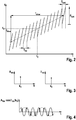
In Fig. 2 the frequency f of a transmission signal is shown over the time t, in the form of a sequence of (fast) frequency ramps (chirps), each of which has a stroke F _fast and a time duration T _almost . The individual frequency _ramps follow one another with a time interval T _r2r ("ramp-to-ramp"). In the in Fig. 2 The example shown is T _almost equal to T _r2r , so that the individual frequency _ramps follow one another directly.

Fig. 2 shows a general representation in which the center frequency of the individual frequency ramps changes in the course of the sequence. In particular, the center frequency of the fast ramps in turn describes a linear frequency ramp with the center frequency f ₀ at time t ₀ . This frequency ramp is also referred to below as a slow ramp. It has a frequency _swing F _slow with a _{ramp duration} T _slow = (N _slow -1) ^∗ T _r2r , where N _slow denotes the number of fast ramps.

In the event that the slow ramp has the frequency swing 0, the fast ramps of the sequence are identical, i.e. describe identical frequency profiles.

Two or more different sequences of fast ramps are used in a measuring cycle, the fast ramps (chirps) each having the same frequency deviation F _almost and the same _{ramp duration} T _almost and the same time interval T _r2r between the ramps within the respective sequence. The at least two sequences within a measurement cycle can vary by different values of the amount and / or the sign of the frequency F, for example, _almost the fast ramps, ramp different durations of the fast ramps, different Rampenwiederholzeiten T _r2r the fast ramps, different Center frequencies f _{0 of} the slow ramps, different number N _{slow of} the fast ramps and / or different frequency _sweeps F _{slow of} the slow ramp.

In order to simplify the representation, the evaluation of the measurement signal for a single sequence of fast ramps of the transmission signal is first explained below.

The frequency of the transmission signal is, for example, in the range of 76 GHz. For example, the center frequency of the slow ramp can be 76 GHz.

In the baseband signal supplied by the mixer 28, each fast ramp is subsequently assigned a partial signal with the duration T _almost . It can be assumed that the signal transit time for a radar object in the detection range of the radar sensor system is short compared to the ramp duration T _almost .

In a first step of the evaluation, a frequency spectrum of at least one partial signal is evaluated. The sub-signal of the baseband signal, which corresponds to a fast ramp, is sampled, ie digitized, at a number N of _almost equidistant times, and a frequency spectrum of the sub-signal is determined. The frequency spectrum is calculated, for example, by calculating a fast Fourier transform (FFT).

Fig. 3 schematically shows the amplitude A _bb and the phase χ _{bb of} the signal obtained in polar coordinates plotted over the frequency bin k.

For a signal reflected by an individual radar object, for example, a peak with the amplitude A _bb (k _o ) is obtained in the frequency bin k ₀ , to which a corresponding phase χ _bb (k _o ) is assigned. The frequency bin k _o identifies the frequency position of the radar object in the relevant frequency spectrum of the partial signal.

wobei c die Lichtgeschwindigkeit ist, D_0,r der Objektabstand zum Mittenzeitpunkt der r-ten Rampe ist, mit r = 1,2, ...,N_slow, und wobei f_0,r die Mittenfrequenz der r-ten Rampe und V_0,r die Relativgeschwindigkeit des Radarobjektes am Mittenzeitpunkt der r-ten schnellen Rampe ist. Die ermittelte Frequenzlage des Peaks entspricht somit einer linearen Beziehung zwischen der Relativgeschwindigkeit V und dem Abstand D des Radarobjektes. Diese Beziehung stellt eine erste Information über die Relativgeschwindigkeit und den Abstand des Radarobjektes dar. Sie ist insbesondere abhängig vom Rampenhub F_fast, der Rampendauer T_fast und der Mittenfrequenz f_0,r der schnellen Rampen.In the case of a linear frequency modulation of the transmission signal, the frequency position of a peak assigned to a radar object is composed of a sum of two terms, of which the first term is proportional to the product of the distance D of the Radar object from the radar sensor and the ramp stroke F is _almost and the second term is proportional to the product of the relative speed V of the radar object, the center frequency of the fast ramp and the ramp duration T is _almost . This corresponds to the FMCW equation $${\mathrm{k}}_{\mathrm{O}}=\left(2/\mathrm{<figure-callout\; id="0"\; label="c\; D"\; filenames="imgf0001.png,imgf0003.png"\; state="\{\{state\}\}">c\; </figure-callout>}\right)\left({\mathrm{D}}_{}\right)\left({\mathrm{}}_{0.\mathrm{r}}{\mathrm{F}}_{\mathrm{nearly}}+{\mathrm{<figure-callout\; id="0"\; label="f"\; filenames="imgf0001.png,imgf0003.png"\; state="\{\{state\}\}">f</figure-callout>}}_{0.\mathrm{r}}{\mathrm{<figure-callout\; id="0"\; label="V"\; filenames="imgf0001.png,imgf0003.png"\; state="\{\{state\}\}">V</figure-callout>}}_{0.\mathrm{r}}{\mathrm{T}}_{\mathrm{nearly}}\right).$$

where c is the speed of light, D _{0, r is} the object distance at the center time of the r-th ramp, with r = 1,2, ..., N _slow , and where f _{0, r is} the center frequency of the r-th ramp and V _{0, r is} the relative speed of the radar object at the midpoint of the rth fast ramp. The determined frequency position of the peak thus corresponds to a linear relationship between the relative speed V and the distance D of the radar object. This relationship represents a first piece of information about the relative speed and the distance of the radar object. It is in particular dependent on the ramp stroke F _fast , the ramp duration T _almost and the center frequency f _{0, r of} the fast ramps.

If the relative speeds V and accelerations of a radar object are not too high, the sequence of the fast ramps results in approximately the same frequency position of the peak, and in the following k ₀ shall denote this mean frequency bin of the radar object over all fast ramps of the sequence.

The phase χ _bb (k _o ) associated with the peak at the frequency position k ₀ is particularly sensitive to changes in the distance of the radar object while passing through the sequence of fast ramps. A change in distance by half the wavelength of the radar signal already results in a phase shift by an entire period of the oscillation.

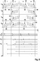
bei der Frequenzlage k₀ des Radarobjektes in den Frequenzspektren während des Verlaufs der Folge der schnellen Rampen. Die in durchgezogenen Linien dargestellte harmonische Schwingung entspricht dabei einem Fall ohne Beschleunigung des Radarobjektes. Fig. 4 shows schematically with a solid line the temporal course of the real part of the spectrum corresponding to a harmonic oscillation $${\mathrm{A}}_{\mathrm{bb}}*{\mathrm{cos\chi }}_{\mathrm{bb}}\left({\mathrm{k}}_{\mathrm{O}}\right)$$

at the frequency position k _{0 of} the radar object in the frequency spectra during the course of the sequence of fast ramps. The harmonic oscillation shown in solid lines corresponds to a case without acceleration of the radar object.

At a radar signal frequency of approximately 76 GHz, the wavelength is approximately 4 mm. At a relative speed of 86 km / h, corresponding to 24 m / sec, the phase changes with a frequency of 12000 Hz. A peak corresponding to this frequency is expected in the frequency spectrum of the temporal course of the real part, the temporal course of the successive fast ramps corresponds; each ramp corresponds to a sample of the course over time. If the Nyquist-Shannon sampling theorem is violated by a sampling frequency of the phase changes that is too low, ie a _{ramp follow-up time} T _r2r , the frequency of the phase changes cannot be clearly determined.

Fig. 4 schematically shows such a subsampling. The values of the real part at the middle times of the respective fast ramps are marked. It cannot be decided whether the true frequency of the phase changes is indicated by the curve drawn in solid lines or by the curve drawn in dashed lines. The frequency is therefore ambiguous.

The frequency position of the harmonic oscillation corresponding to the phase change can be determined by subjecting the function, which indicates the phase χ _bb (r) measured for an object as a function of the ramp index r, to a Fourier transformation again. This frequency position can be indicated by its frequency bin I ₀ and is approximately additively composed of a term proportional to the mean distance D and the ramp stroke F _{slow of} the slow ramp and a term related to the mean relative speed V, the ramp duration T _{slow of} the slow ramp and the center frequency f ₀ is proportional to the slow ramp. This in turn corresponds to an FMCW equation for the slow ramp: $${\mathrm{I}}_0=\left(2/\mathrm{c}\right)\left(\mathrm{D}{\mathrm{F}}_{\mathrm{slow}}+\mathrm{V}{\mathrm{T}}_{\mathrm{slow}}{\mathrm{f}}_{\mathrm{O}}\right),$$

In the general case, ie with a ramp stroke of the slow ramp F _slow ≠ 0, the determined frequency position thus results in a linear relationship between the relative speed and the distance of the radar object, which, however, is ambiguous with regard to the relative speed V and the distance D. This relationship represents a second piece of information about the relative speed and the distance of the radar object. In the special case F _slow = 0, the term “slow ramp” is used in the following; this has the slope 0 and gives second information only about the speed. _With regard to the relative speed V, this is unambiguous except for integral multiples of the product of half the wavelength and the sampling frequency 1 / T _{r2r of} the slow ramp.

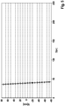
Fig. 5 shows by way of example the information about the relative speed V and the distance D resulting from the evaluation of the measurement signal for a sequence of frequency ramps. The parameters of the frequency modulation are the following: F _fast = 425 MHz, T _fast = 0.25 ms, each fast ramp is sampled at N _almost = 512 sampling times, the frequency deviation of the slow ramp is F _slow = 0, the time interval of the fast ramps is T _r2r = 0.25 ms, the number of fast ramps, ie the number of sampling times of the slow ramp, is N _slow = 16, so that the duration of the slow ramps is T _slow = 4 ms. The detected radar object has a distance of d = 40 m and a relative speed v = -20 m / s.

The evaluation of a frequency spectrum of a partial signal results in a straight line inclined with respect to the vertical, corresponding to a linear relationship between the relative speed V and the distance D. Since the ramp stroke of the slow ramp F is _slow = 0, the values are obtained from the Fourier analysis the frequency spectra of the partial signals at the frequency position k _{0 of} the radar object is an ambiguous value for the relative speed V, corresponding to the horizontal, dashed lines in the diagram in FIG Fig. 5 , This ambiguous value represents the second information about the relative speed. Linking the first information with the second information, taking into account the ambiguity mentioned, results in potential value pairs (V, D). These are in Fig. 5 marked with circles that have a tolerance range Illustrate for making the comparison. The real target at V = -20 m / s is marked by an asterisk.

The determination of the relative speed and distance of the radar object can be made unambiguous by taking further first information about relative speed and distance and / or further second information about relative speed and optionally distance into account.

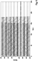
Fig. 6 illustrates schematically a clear determination of relative speeds and distances of radar objects when using two different modulation patterns in each measurement cycle.

The parameters of the first modulation pattern are the following: F _fast = 425 MHz, T _fast = 0.10 ms, N _fast = 1024, F _slow = 0, T _r2r = 0.10 ms, N _slow = 32, so that T _slow = 3.2 ms results.

The parameters of the second modulation pattern are the following: F _fast = -250 MHz, T _fast = 0.115 ms, N _fast = 512, F _slow = 0, T _r2r = 0.115 ms, N _slow = 32, so that T _slow = 3 , 68 ms results.

In this example, it is assumed that a number of radar objects are present at a relative speed of V = -30 m / s in the distance range from D = 5 m to D = 250 m, the radar objects being at a distance of 5 m from one another. For example, these can be standing targets to which one's own motor vehicle is moving at a speed of 30 m / s.

The linear relationships between V and D differ for the two modulation patterns. The first modulation pattern provides a family of parallel, falling lines, one line for each object. The second modulation pattern accordingly provides a family of rising straight lines. Furthermore, the second information about the speed V of the radar object determined from the two modulation patterns has different ambiguity ranges.

In Fig. 6 are the intersections of the straight lines as in Fig. 5 marked with circles. The signals obtained from the two modulation patterns are compared by looking for those values for the relative speed V and the distance D for which the straight line intersections provided by the two modulation patterns best match. In the example shown, the relative speed V = -30 m / s is obtained for all objects.

The chain of standing radar objects at a relative speed of V = -30 m / s can be resolved and detected up to a distance of 150 m.

In order to make the method more robust to situations in which several objects with different relative speeds are located at the same time, it is advisable not only to work with two different modulation patterns, but with at least three different modulation patterns per measurement cycle.

In order to achieve a shorter cycle time, however, a cycle scheme is preferably used that in Fig. 7 is shown. There (for the sake of simplicity for slow ramps with zero slope) the frequency f of the transmission signal is plotted against time t for two complete measuring cycles P. In each measuring cycle P, the frequency is modulated according to three different modulation patterns M ₁ , M ₂ and M ₃ . Each modulation pattern is followed by a computing time interval of length T, within which the baseband signal obtained for the modulation pattern in question is evaluated.

The results obtained for the last three modulation patterns are also compared within each computing time interval. In Fig. 7 this is symbolically represented for the computing time intervals in the second measuring cycle. This measuring cycle contains three sub-cycles Z ₁ , Z ₂ and Z ₃ . In sub-cycle Z ₁ , the result (the family of straight lines in the VD diagram) obtained for the modulation pattern M ₁ in the current measurement cycle is compared with the results obtained for the modulation patterns M ₂ and M ₃ in the previous two Has received partial cycles (within the previous measuring cycle P). Through this comparison you get for each object has a unique pair of values for distance and relative speed that can be output at the end of this sub-cycle. Correspondingly, in sub-cycle Z _2, the result obtained for the modulation pattern M ₂ in this sub-cycle is compared with the result for the immediately preceding modulation pattern M ₁ and the preceding modulation pattern M ₃ . The same procedure is followed for sub-cycle Z ₃ .

In this way, updated values for the distance and the relative speed of each object are obtained after a cycle time which is composed only of the duration of a single modulation pattern and the computing time T.

The following will now refer to Fig. 1 . 7 and 8th the MIMO principle and its combination with the MSFMCW method described above are explained.

As in Fig. 1 Based on the radar beams is shown schematically, the different positions of the antenna elements 10-16 lead to the fact that the radar beams, which were emitted by one and the same antenna element, were reflected on the object and then received by the different antenna elements, cover different run lengths and therefore phase differences exhibit. that depend on the azimuth angle θ of the object. The associated intermediate frequency signals Zf ₁ - Zf _{4 also} have corresponding phase differences. The amplitudes (amounts) of the received signals also differ from antenna element to antenna element, likewise depending on the azimuth angle θ. The dependence of the complex amplitudes, ie the absolute amounts and phases, of the received signals on the azimuth angle θ can be stored in the control and evaluation unit 30 for each antenna element in the form of an antenna diagram. An angle estimator 38 compares the complex amplitudes obtained in the four receiving channels with the antenna diagrams for each located object (each peak in the frequency spectrum), so as to estimate the azimuth angle θ of the object. The most likely value for the azimuth angle is assumed to be the value at which the measured It is best to correlate amplitudes with the values read in the antenna diagrams.

In the MIMO radar described here, however, the complex amplitudes in the four channels also depend on which of the four antenna elements 10, 12, 14, 16 is used as the transmission element. For example, the switching network 22 allows a first frequency ramp or sequence of frequency ramps to be transmitted with the antenna element 10 (the transmission array then consists only of the single antenna element 10), then to switch over to the antenna element 12 and then successively to the antenna elements 14 and 16, after which a new cycle begins. In this way you get 4 x 4 = 16 different constellations, which can be described by the following signal model.

For the planar linear antenna array with the antenna elements 10, 12, 14, 16 as the receiving array, the control _vector a _rµ (θ) has the following components (assuming idealized isotropic antenna elements): $${\mathrm{a}}_{\mathrm{r\mu }}\left(\mathrm{\theta }\right)=\mathrm{<figure-callout\; id="2"\; label="exp"\; filenames="imgf0006.png"\; state="\{\{state\}\}">exp</figure-callout>}\left(2\mathrm{\pi }\mathrm{i}\cdot \left({\mathrm{d}}_{\mathrm{r\mu }}/\mathrm{\lambda }\right)\cdot \sin \left(\mathrm{\theta }\right)\right).\mathrm{\mu }=1.....4$$

This control vector determines the phase relationships between the complex amplitudes of the signals received by the four antenna elements. The index µ denotes the antenna element, and the sizes d _rµ indicate the positions of the antenna elements in the horizontal, based on any arbitrarily selected origin.

Accordingly, the control _vector a _tν (θ) for the receiving array has the components $${\mathrm{a}}_{\mathrm{t\nu }}\left(\mathrm{\theta }\right)=\mathrm{<figure-callout\; id="2"\; label="exp"\; filenames="imgf0006.png"\; state="\{\{state\}\}">exp</figure-callout>}\left(2\mathrm{\pi }\mathrm{i}\cdot \left({\mathrm{d}}_{\mathrm{t\nu }}/\mathrm{\lambda }\right)\cdot \sin \left(\mathrm{\theta }\right)\right).\mathrm{\nu }=1,\; ...,4,$$

$${\mathrm{d}}_{\mathrm{r}2}={\mathrm{d}}_{\mathrm{t}2}={\mathrm{d}}_2,$$

$${\mathrm{d}}_{\mathrm{r}3}={\mathrm{d}}_{\mathrm{t}3}={\mathrm{d}}_3$$

und $${\mathrm{d}}_{\mathrm{r}4}={\mathrm{d}}_{\mathrm{t}4}={\mathrm{d}}_4.$$

At the in Fig. 1 The example of a monostatic array with four antenna elements shown can take the location of the antenna element 10 as the coordinate origin, so that: $${\mathrm{<figure-callout\; id="1"\; label="d\; r"\; filenames="imgf0006.png,imgf0007.png"\; state="\{\{state\}\}">d\; </figure-callout>}}_{\mathrm{r}}={\mathrm{<figure-callout\; id="1"\; label="d\; t"\; filenames="imgf0006.png,imgf0007.png"\; state="\{\{state\}\}">d\; </figure-callout>}}_{\mathrm{t}}=0.$$

$${\mathrm{d}}_{\mathrm{<figure-callout\; id="2"\; label="r"\; filenames="imgf0006.png"\; state="\{\{state\}\}">r</figure-callout>}2}={\mathrm{<figure-callout\; id="2"\; label="d\; t"\; filenames="imgf0006.png"\; state="\{\{state\}\}">d\; </figure-callout>}}_{\mathrm{t}}={\mathrm{<figure-callout\; id="2"\; label="d"\; filenames="imgf0006.png"\; state="\{\{state\}\}">d</figure-callout>}}_2.$$

$${\mathrm{d}}_{\mathrm{r}3}={\mathrm{d}}_{\mathrm{t}3}={\mathrm{d}}_3$$

and $${\mathrm{d}}_{\mathrm{r}4}={\mathrm{d}}_{\mathrm{t}4}={\mathrm{d}}_4,$$

For the angle _estimation, the virtual array vector is now formed according to the MIMO principle, in that the Kronecker product is formed from a _tν (θ) and a _rµ (θ): $$\mathrm{a}\left(\mathrm{\theta }\right)=\left({\mathrm{a}}_{\mathrm{<figure-callout\; id="1"\; label="t"\; filenames="imgf0006.png,imgf0007.png"\; state="\{\{state\}\}">t</figure-callout>}1}\left(\mathrm{\theta }\right)\cdot {\mathrm{a}}_{\mathrm{<figure-callout\; id="1"\; label="r"\; filenames="imgf0006.png,imgf0007.png"\; state="\{\{state\}\}">r</figure-callout>}1}\left(\mathrm{\theta }\right).{\mathrm{a}}_{\mathrm{<figure-callout\; id="1"\; label="t"\; filenames="imgf0006.png,imgf0007.png"\; state="\{\{state\}\}">t</figure-callout>}1}\left(\mathrm{\theta }\right)\cdot {\mathrm{a}}_{\mathrm{<figure-callout\; id="2"\; label="r"\; filenames="imgf0006.png"\; state="\{\{state\}\}">r</figure-callout>}2}\left(\mathrm{\theta }\right).{\mathrm{a}}_{\mathrm{<figure-callout\; id="1"\; label="t"\; filenames="imgf0006.png,imgf0007.png"\; state="\{\{state\}\}">t</figure-callout>}1}\left(\mathrm{\theta }\right)\cdot {\mathrm{a}}_{\mathrm{r}3}\left(\mathrm{\theta }\right).{\mathrm{a}}_{\mathrm{<figure-callout\; id="1"\; label="t"\; filenames="imgf0006.png,imgf0007.png"\; state="\{\{state\}\}">t</figure-callout>}1}\left(\mathrm{\theta }\right)\cdot {\mathrm{a}}_{\mathrm{r}4}\left(\mathrm{\theta }\right).{\mathrm{a}}_{\mathrm{<figure-callout\; id="2"\; label="t"\; filenames="imgf0006.png"\; state="\{\{state\}\}">t</figure-callout>}2}\left(\mathrm{\theta }\right)\cdot {\mathrm{a}}_{\mathrm{<figure-callout\; id="1"\; label="r"\; filenames="imgf0006.png,imgf0007.png"\; state="\{\{state\}\}">r</figure-callout>}1}\left(\mathrm{\theta }\right).{\mathrm{a}}_{\mathrm{<figure-callout\; id="2"\; label="t"\; filenames="imgf0006.png"\; state="\{\{state\}\}">t</figure-callout>}2}\left(\mathrm{\theta }\right)\cdot {\mathrm{a}}_{\mathrm{<figure-callout\; id="2"\; label="r"\; filenames="imgf0006.png"\; state="\{\{state\}\}">r</figure-callout>}2}\left(\mathrm{\theta }\right).{\mathrm{a}}_{\mathrm{<figure-callout\; id="2"\; label="t"\; filenames="imgf0006.png"\; state="\{\{state\}\}">t</figure-callout>}2}\left(\mathrm{\theta }\right)\cdot {\mathrm{a}}_{\mathrm{r}3}\left(\mathrm{\theta }\right).{\mathrm{a}}_{\mathrm{<figure-callout\; id="2"\; label="t"\; filenames="imgf0006.png"\; state="\{\{state\}\}">t</figure-callout>}2}\left(\mathrm{\theta }\right)\cdot {\mathrm{a}}_{\mathrm{r}4}\left(\mathrm{\theta }\right).{\mathrm{a}}_{\mathrm{t}3}\left(\mathrm{\theta }\right)\cdot {\mathrm{a}}_{\mathrm{<figure-callout\; id="1"\; label="r"\; filenames="imgf0006.png,imgf0007.png"\; state="\{\{state\}\}">r</figure-callout>}1}\left(\mathrm{\theta }\right).{\mathrm{a}}_{\mathrm{t}3}\left(\mathrm{\theta }\right)\cdot {\mathrm{a}}_{\mathrm{<figure-callout\; id="2"\; label="r"\; filenames="imgf0006.png"\; state="\{\{state\}\}">r</figure-callout>}2}\left(\mathrm{\theta }\right).{\mathrm{a}}_{\mathrm{t}3}\left(\mathrm{\theta }\right)\cdot {\mathrm{a}}_{\mathrm{r}3}\left(\mathrm{\theta }\right).{\mathrm{a}}_{\mathrm{t}3}\left(\mathrm{\theta }\right)\cdot {\mathrm{a}}_{\mathrm{r}4}\left(\mathrm{\theta }\right).{\mathrm{a}}_{\mathrm{t}4}\left(\mathrm{\theta }\right)\cdot {\mathrm{a}}_{\mathrm{<figure-callout\; id="1"\; label="r"\; filenames="imgf0006.png,imgf0007.png"\; state="\{\{state\}\}">r</figure-callout>}1}\left(\mathrm{\theta }\right).{\mathrm{a}}_{\mathrm{t}4}\left(\mathrm{\theta }\right)\cdot {\mathrm{a}}_{\mathrm{<figure-callout\; id="2"\; label="r"\; filenames="imgf0006.png"\; state="\{\{state\}\}">r</figure-callout>}2}\left(\mathrm{\theta }\right).{\mathrm{a}}_{\mathrm{t}4}\left(\mathrm{\theta }\right)\cdot {\mathrm{a}}_{\mathrm{r}3}\left(\mathrm{\theta }\right).{\mathrm{a}}_{\mathrm{t}4}\left(\mathrm{\theta }\right)\cdot {\mathrm{a}}_{\mathrm{r}4}\left(\mathrm{\theta }\right)\right)$$

The product vector has sixteen components, corresponding to sixteen positions of virtual antenna elements. The components of the vector have the shape $${\mathrm{a}}_{\mathrm{t\nu }}\left(\mathrm{\theta }\right)\cdot {\mathrm{a}}_{\mathrm{r\mu }}\left(\mathrm{\theta }\right)=\mathrm{<figure-callout\; id="2"\; label="exp"\; filenames="imgf0006.png"\; state="\{\{state\}\}">exp</figure-callout>}\left(2\mathrm{\pi }\mathrm{i}\cdot \left(\left({\mathrm{d}}_{\mathrm{t\nu }}+{\mathrm{d}}_{\mathrm{r\mu }}\right)/\mathrm{\lambda }\right)\cdot \sin \left(\mathrm{\theta }\right)\right);\mathrm{\nu }=1.....4;\mathrm{\mu }=1.....4$$

The virtual antenna positions thus correspond to the sums that can be formed from the quantities d ₁ - d ₄ . The virtual array thus extends horizontally over a much larger span, that is, it has a larger aperture and thus leads to a higher angular resolution, since even small changes in the azimuth angle θ lead to larger phase differences.

However, if the values d ₁ - d ₄ are chosen to be significantly larger than λ / 2 in order to obtain the largest possible aperture, then due to the periodicity of the factor sin (θ) Azimuth angles occur in individual cases in the components of the array vector, in which the antenna diagrams have similar complex amplitudes for all virtual antenna elements, so that the real azimuth angle of the object cannot be clearly determined.

The virtual array is therefore preferably filled up by additional virtual elements. For this purpose, the switching network 22 is controlled in certain operating phases in such a way that two switches are closed simultaneously, that is to say two associated antenna elements 10, 12, 14, 16 are simultaneously fed with the same signal. The transmitted signals then overlap to form a signal whose wave pattern has approximately the shape as if it originated from a point in the middle between the relevant antenna elements.

For example, if the antenna elements are fed together 10 and 12, one obtains in the control vector for the transmit array one additional component exp (2πi · (d ₂ / 2λ) · sin (θ)) corresponding to an additional antenna element in the position of d _2/2. In the vector of the virtual array, the four additional components, corresponding virtual elements results in the positions d _2/2, d _2/2 + d _2, d _2/2 + d ₃ and d _2/2 + d. ₄ For the true azimuth angle of the object, the antenna diagrams belonging to these virtual elements must also supply the complex amplitudes of the intermediate frequency signals Zf ₁ -Zf ₄ measured for the peak of the object. In this way, the additional elements help to avoid any ambiguity.

In practice, not all possible combinations of the antenna elements 10 - 16 have to be used as transmission arrays, but rather a sensible selection is made. An example of a possible mode of operation is shown in diagram form in Fig. 8 shown.

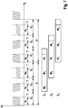
In the upper part of the diagram, the frequencies f ₁ - f ₄ of the signals transmitted by the antenna elements 10 - 16 are plotted as a function of the time t. In a first period 1 only the antenna elements 10 and 16 are active and they send signals (frequencies f ₁ and f ₄ ) which consist of a rising slow frequency ramp 40, 42 with chirps 44, 46. The chirps 44 and 46 alternate with one another without to overlap each other in time. An overlay of the transmitted signals is avoided. The first chirp 46, which is transmitted with the antenna element 16, has the same frequency position and the same stroke as the first chirp 44, which is transmitted with the antenna element 10. So the two chirps are identical copies or repetitions. The same applies to each subsequent pair of chirps 44, 46. The sequences of chirps 44, 46 are generated in this example by the oscillator 24, which is alternately connected to the antenna elements 10 and 16 by the switching network 22.

In a second period 2, the frequency ramps 40, 42 are repeated. However, the switching network 22 now connects the oscillator to the two antenna elements 10 and 12 during the chirps 44 and to the two antenna elements 14 and 16 during the chirps 46, so that the transmit array in each case consists of a pair of adjacent antenna elements.

In subsequent periods 3 and 4, slow frequency ramps 48, 50 falling with chirps 52, 54 are transmitted according to the same scheme. This completes a complete measurement cycle, which in this simplified example contains only two modulation patterns (a rising and a falling slow ramp).

In the lower part of the diagram, the positions d of the transmitting antenna elements (bold angles) and the positions of the respective virtual antenna elements (thinner angles) are symbolically shown for each period. In the first period, the virtual positions for the chirps 44 match the real positions. For the chirps 46, the positions are offset by d ₄ , since the antenna element 16 transmits which is offset by this distance from the antenna element 10.

In the subsequent period 2, the transmit array for the chirps 44 has the same effect as an array with a single antenna element at the position d _2/2, and the transmit array for the chirps 46 has the same effect as an array with a single antenna element in the Position (d ₃ + d ₄ ) / 2. The virtual positions in periods 3 and 4 also result in the same way.

In the far right column in the lower part of the diagram in Fig. 8 all the virtual positions of the antenna elements obtained in this way are shown together. It can be seen that the virtual array is filled to a high degree with additional virtual elements, so that not only a high angular resolution (corresponding to the large aperture) is obtained, but also a high degree of uniqueness (due to the density of the virtual elements within the arrays).

$${\mathrm{d}}_2=\mathrm{1,2}$$

$${\mathrm{d}}_3=\mathrm{5,5}$$

$${\mathrm{d}}_4=\mathrm{10,2}$$

If the antenna elements 10-16 were evenly spaced, the positions of some of the virtual antenna elements would coincide. However, in the embodiment shown this is avoided by the fact that the distances between the antenna elements are unequal: d ₄ - d ₃ > d ₃ - d ₂ > d ₂ . The following values have proven themselves in practice (in units of wavelength λ): $${\mathrm{<figure-callout\; id="1"\; label="d"\; filenames="imgf0006.png,imgf0007.png"\; state="\{\{state\}\}">d</figure-callout>}}_1=0$$

$${\mathrm{<figure-callout\; id="2"\; label="d"\; filenames="imgf0006.png"\; state="\{\{state\}\}">d</figure-callout>}}_2=1.2$$

$${\mathrm{d}}_3=5.5$$

$${\mathrm{d}}_4=10.2$$

An antenna diagram can be created for each of the virtual arrays, which indicates the amplitude and / or phase relationships of the signals received in the four evaluation channels as a function of the assumed angle of incidence θ of the radar echo. In general, the azimuth angle of the located object, i.e. the actual angle of incidence α, will correspond to the assumed angle of incidence θ for which there is the best match between the amplitude and / or phase relationships actually measured in the evaluation channels and the corresponding values in the antenna diagram. For the evaluation, a DML function (Deterministic Maximum Likelihood) can be calculated, which indicates the correlation between the actually measured values and the values in the antenna diagram as a function of the angle of incidence θ. The function value of the DML function varies between 0 (no correlation) and 1 (complete agreement). The four in this example Evaluation channels of measured amplitudes and / or phases (complex amplitudes) can be understood as a four-component vector. Accordingly, the values in the antenna diagrams form a four-component vector for each angle of incidence θ. The DML function can then be calculated by normalizing these two vectors to 1 and then forming the dot product or the amount of the dot product or the square of the amount. The maximum of the DML function then provides the best estimate for the azimuth angle of the object.

To determine these estimates, the angle estimator 38 forms the four-component amplitude vector for each of the chirps 44, 52 and for each peak found therein (that is to say for each localized object) and calculates the DML function using the antenna diagrams for the virtual array that occurs in periods 1 and 3 is used. Correspondingly, for chirps 46 and 54, the DML function is calculated on the basis of the antenna diagrams for the virtual array that is used in periods 2 and 4.

In 9 (a) and (b) Examples of these two DML functions are shown, each assuming that the radar radiation is incident from the front (actual angle of incidence α = 0 °) and the received signals are noiseless. The upper diagram (a) shows the DML function for periods 2 and 4, and diagram (b) shows the DML function for periods 1 and 3. As expected, these functions have a main maximum at θ = 0 however also secondary maxima at other angles.

The diagram (c) in Fig. 9 shows the DML function, which corresponds to a combination (a weighted sum) of the diagrams (a) and (b). In this example, the diagram (a) is weighted twice, because in the associated switching states, two antenna elements (10 and 12 or 14 and 16) are sent simultaneously. However, other types of weighting and other forms of combination (e.g. median) are also conceivable.

It can be seen that there is only a sharply defined maximum at θ = 0 in this sum, while the other maxima are suppressed to such an extent that they do not reach the value 1 even taking the noise into account.

For other values of the actual angle of incidence α, one would obtain other (asymmetrical) DML functions in which the maxima are at different locations. Each function would then have a main maximum at θ = α.

Claims (7)

1. Angle-resolving FMCW radar sensor having a plurality of antenna elements (10, 12, 14, 16) which are arranged at different positions in a direction in which the radar sensor is angle-resolving and form at least three transmitting arrays and at least one receiving array, wherein a transmitting array can consist of an individual antenna element or of a combination of a plurality of antenna elements, and having a control and evaluation device (30) which is designed for a method of operation in which the at least three transmitting arrays periodically transmit signals, the frequency of which is modulated according to a sequence of modulation ramps (44, 46; 52, 54), and in which radar echoes of the transmitted signals are respectively received by a plurality of antenna elements in the at least one receiving array and the angle (θ) of a located object is determined on the basis of amplitude and/or phase relationships between radar echoes corresponding to different combinations of transmitting and receiving arrays, characterized in that a measuring cycle (P) of the radar sensor comprises at least two periods (1, 2, 3, 4) in which there is respectively a change between at least two combinations of transmitting and receiving arrays and there is a change back in further periods, and in that the involved combinations of transmitting and receiving arrays differ from one another for the at least two periods.
2. Radar sensor according to Claim 1, in which each period (1, 2, 3, 4) contains a sequence of modulation ramps (44, 46; 52, 54) and there is a changeover to a different transmitting array after each individual modulation ramp.
3. Radar sensor according to Claim 1 or 2, in which there is alternately a changeover between two transmitting arrays within an individual period (1, 2, 3, 4) .
4. Radar sensor according to one of the preceding claims, in which at least one of the transmitting arrays which is used for transmission in at least one period (1, 3) consists of an individual antenna element (10; 16) and at least one other transmitting array which is used for transmission in at least one period (2, 4) consists of at least two antenna elements (10, 12; 14, 16) which are simultaneously fed with signals of the same frequency.
5. Radar sensor according to one of the preceding claims, in which each of the antenna elements (10, 12, 14, 16) can be optionally operated as part of a receiving array and as part of a transmitting array.
6. Radar sensor according to one of the preceding claims, in which the antenna elements (10, 12, 14, 16) which can be operated as part of a transmitting array have different distances from neighbour to neighbour.
7. Radar sensor according to one of the preceding claims, in which, in order to determine the distance (D) of a located object, differences in the phase angles of received radar echoes which belong to different modulation patterns (M₁, M₂, M₃) are evaluated, and in which, in order to identify the radar echoes of a plurality of simultaneously located objects, the results obtained for a plurality of successive modulation patterns are compared with one another, wherein at least one of these modulation patterns respectively comes from a preceding measuring cycle (P).

Images