EP2933502B1 - Digital hydraulic drive system - Google Patents
Digital hydraulic drive system Download PDFInfo
- Publication number
- EP2933502B1 EP2933502B1 EP15000306.9A EP15000306A EP2933502B1 EP 2933502 B1 EP2933502 B1 EP 2933502B1 EP 15000306 A EP15000306 A EP 15000306A EP 2933502 B1 EP2933502 B1 EP 2933502B1
- Authority
- EP
- European Patent Office
- Prior art keywords
- control
- drive system
- valve
- actuator
- flatness
- Prior art date
- Legal status (The legal status is an assumption and is not a legal conclusion. Google has not performed a legal analysis and makes no representation as to the accuracy of the status listed.)
- Active
Links
- 238000013461 design Methods 0.000 claims description 12
- 238000006073 displacement reaction Methods 0.000 claims description 6
- 230000001419 dependent effect Effects 0.000 claims description 2
- 230000001105 regulatory effect Effects 0.000 claims 1
- 239000012530 fluid Substances 0.000 description 8
- 230000015654 memory Effects 0.000 description 8
- 230000006870 function Effects 0.000 description 6
- 230000006399 behavior Effects 0.000 description 5
- 238000000034 method Methods 0.000 description 5
- 238000013459 approach Methods 0.000 description 4
- 230000004888 barrier function Effects 0.000 description 4
- 238000013016 damping Methods 0.000 description 4
- 238000004088 simulation Methods 0.000 description 4
- 230000008901 benefit Effects 0.000 description 3
- OKTJSMMVPCPJKN-UHFFFAOYSA-N Carbon Chemical compound [C] OKTJSMMVPCPJKN-UHFFFAOYSA-N 0.000 description 2
- 230000008859 change Effects 0.000 description 2
- 238000005516 engineering process Methods 0.000 description 2
- 230000005284 excitation Effects 0.000 description 2
- 230000002706 hydrostatic effect Effects 0.000 description 2
- 238000005259 measurement Methods 0.000 description 2
- 230000010355 oscillation Effects 0.000 description 2
- 230000003044 adaptive effect Effects 0.000 description 1
- 238000009530 blood pressure measurement Methods 0.000 description 1
- 238000011217 control strategy Methods 0.000 description 1
- 238000010586 diagram Methods 0.000 description 1
- 238000011156 evaluation Methods 0.000 description 1
- RZTAMFZIAATZDJ-UHFFFAOYSA-N felodipine Chemical class CCOC(=O)C1=C(C)NC(C)=C(C(=O)OC)C1C1=CC=CC(Cl)=C1Cl RZTAMFZIAATZDJ-UHFFFAOYSA-N 0.000 description 1
- 238000013178 mathematical model Methods 0.000 description 1
- 230000008569 process Effects 0.000 description 1
- 230000002787 reinforcement Effects 0.000 description 1
- 230000000717 retained effect Effects 0.000 description 1
- 238000004513 sizing Methods 0.000 description 1
- 230000003068 static effect Effects 0.000 description 1
- 230000001360 synchronised effect Effects 0.000 description 1
- 230000007704 transition Effects 0.000 description 1
- 238000011144 upstream manufacturing Methods 0.000 description 1
Images


Classifications
-
- F—MECHANICAL ENGINEERING; LIGHTING; HEATING; WEAPONS; BLASTING
- F15—FLUID-PRESSURE ACTUATORS; HYDRAULICS OR PNEUMATICS IN GENERAL
- F15B—SYSTEMS ACTING BY MEANS OF FLUIDS IN GENERAL; FLUID-PRESSURE ACTUATORS, e.g. SERVOMOTORS; DETAILS OF FLUID-PRESSURE SYSTEMS, NOT OTHERWISE PROVIDED FOR
- F15B11/00—Servomotor systems without provision for follow-up action; Circuits therefor
- F15B11/02—Systems essentially incorporating special features for controlling the speed or actuating force of an output member
- F15B11/04—Systems essentially incorporating special features for controlling the speed or actuating force of an output member for controlling the speed
- F15B11/042—Systems essentially incorporating special features for controlling the speed or actuating force of an output member for controlling the speed by means in the feed line, i.e. "meter in"
- F15B11/0426—Systems essentially incorporating special features for controlling the speed or actuating force of an output member for controlling the speed by means in the feed line, i.e. "meter in" by controlling the number of pumps or parallel valves switched on
-
- F—MECHANICAL ENGINEERING; LIGHTING; HEATING; WEAPONS; BLASTING
- F15—FLUID-PRESSURE ACTUATORS; HYDRAULICS OR PNEUMATICS IN GENERAL
- F15B—SYSTEMS ACTING BY MEANS OF FLUIDS IN GENERAL; FLUID-PRESSURE ACTUATORS, e.g. SERVOMOTORS; DETAILS OF FLUID-PRESSURE SYSTEMS, NOT OTHERWISE PROVIDED FOR
- F15B11/00—Servomotor systems without provision for follow-up action; Circuits therefor
- F15B11/02—Systems essentially incorporating special features for controlling the speed or actuating force of an output member
- F15B11/04—Systems essentially incorporating special features for controlling the speed or actuating force of an output member for controlling the speed
- F15B11/044—Systems essentially incorporating special features for controlling the speed or actuating force of an output member for controlling the speed by means in the return line, i.e. "meter out"
-
- F—MECHANICAL ENGINEERING; LIGHTING; HEATING; WEAPONS; BLASTING
- F15—FLUID-PRESSURE ACTUATORS; HYDRAULICS OR PNEUMATICS IN GENERAL
- F15B—SYSTEMS ACTING BY MEANS OF FLUIDS IN GENERAL; FLUID-PRESSURE ACTUATORS, e.g. SERVOMOTORS; DETAILS OF FLUID-PRESSURE SYSTEMS, NOT OTHERWISE PROVIDED FOR
- F15B2211/00—Circuits for servomotor systems
- F15B2211/30—Directional control
- F15B2211/305—Directional control characterised by the type of valves
- F15B2211/3056—Assemblies of multiple valves
- F15B2211/30565—Assemblies of multiple valves having multiple valves for a single output member, e.g. for creating higher valve function by use of multiple valves like two 2/2-valves replacing a 5/3-valve
- F15B2211/30575—Assemblies of multiple valves having multiple valves for a single output member, e.g. for creating higher valve function by use of multiple valves like two 2/2-valves replacing a 5/3-valve in a Wheatstone Bridge arrangement (also half bridges)
-
- F—MECHANICAL ENGINEERING; LIGHTING; HEATING; WEAPONS; BLASTING
- F15—FLUID-PRESSURE ACTUATORS; HYDRAULICS OR PNEUMATICS IN GENERAL
- F15B—SYSTEMS ACTING BY MEANS OF FLUIDS IN GENERAL; FLUID-PRESSURE ACTUATORS, e.g. SERVOMOTORS; DETAILS OF FLUID-PRESSURE SYSTEMS, NOT OTHERWISE PROVIDED FOR
- F15B2211/00—Circuits for servomotor systems
- F15B2211/30—Directional control
- F15B2211/32—Directional control characterised by the type of actuation
- F15B2211/327—Directional control characterised by the type of actuation electrically or electronically
-
- F—MECHANICAL ENGINEERING; LIGHTING; HEATING; WEAPONS; BLASTING
- F15—FLUID-PRESSURE ACTUATORS; HYDRAULICS OR PNEUMATICS IN GENERAL
- F15B—SYSTEMS ACTING BY MEANS OF FLUIDS IN GENERAL; FLUID-PRESSURE ACTUATORS, e.g. SERVOMOTORS; DETAILS OF FLUID-PRESSURE SYSTEMS, NOT OTHERWISE PROVIDED FOR
- F15B2211/00—Circuits for servomotor systems
- F15B2211/30—Directional control
- F15B2211/35—Directional control combined with flow control
- F15B2211/351—Flow control by regulating means in feed line, i.e. meter-in control
-
- F—MECHANICAL ENGINEERING; LIGHTING; HEATING; WEAPONS; BLASTING
- F15—FLUID-PRESSURE ACTUATORS; HYDRAULICS OR PNEUMATICS IN GENERAL
- F15B—SYSTEMS ACTING BY MEANS OF FLUIDS IN GENERAL; FLUID-PRESSURE ACTUATORS, e.g. SERVOMOTORS; DETAILS OF FLUID-PRESSURE SYSTEMS, NOT OTHERWISE PROVIDED FOR
- F15B2211/00—Circuits for servomotor systems
- F15B2211/30—Directional control
- F15B2211/35—Directional control combined with flow control
- F15B2211/353—Flow control by regulating means in return line, i.e. meter-out control
-
- F—MECHANICAL ENGINEERING; LIGHTING; HEATING; WEAPONS; BLASTING
- F15—FLUID-PRESSURE ACTUATORS; HYDRAULICS OR PNEUMATICS IN GENERAL
- F15B—SYSTEMS ACTING BY MEANS OF FLUIDS IN GENERAL; FLUID-PRESSURE ACTUATORS, e.g. SERVOMOTORS; DETAILS OF FLUID-PRESSURE SYSTEMS, NOT OTHERWISE PROVIDED FOR
- F15B2211/00—Circuits for servomotor systems
- F15B2211/40—Flow control
- F15B2211/405—Flow control characterised by the type of flow control means or valve
- F15B2211/40576—Assemblies of multiple valves
- F15B2211/40592—Assemblies of multiple valves with multiple valves in parallel flow paths
-
- F—MECHANICAL ENGINEERING; LIGHTING; HEATING; WEAPONS; BLASTING
- F15—FLUID-PRESSURE ACTUATORS; HYDRAULICS OR PNEUMATICS IN GENERAL
- F15B—SYSTEMS ACTING BY MEANS OF FLUIDS IN GENERAL; FLUID-PRESSURE ACTUATORS, e.g. SERVOMOTORS; DETAILS OF FLUID-PRESSURE SYSTEMS, NOT OTHERWISE PROVIDED FOR
- F15B2211/00—Circuits for servomotor systems
- F15B2211/40—Flow control
- F15B2211/41—Flow control characterised by the positions of the valve element
- F15B2211/411—Flow control characterised by the positions of the valve element the positions being discrete
-
- F—MECHANICAL ENGINEERING; LIGHTING; HEATING; WEAPONS; BLASTING
- F15—FLUID-PRESSURE ACTUATORS; HYDRAULICS OR PNEUMATICS IN GENERAL
- F15B—SYSTEMS ACTING BY MEANS OF FLUIDS IN GENERAL; FLUID-PRESSURE ACTUATORS, e.g. SERVOMOTORS; DETAILS OF FLUID-PRESSURE SYSTEMS, NOT OTHERWISE PROVIDED FOR
- F15B2211/00—Circuits for servomotor systems
- F15B2211/40—Flow control
- F15B2211/42—Flow control characterised by the type of actuation
- F15B2211/426—Flow control characterised by the type of actuation electrically or electronically
-
- F—MECHANICAL ENGINEERING; LIGHTING; HEATING; WEAPONS; BLASTING
- F15—FLUID-PRESSURE ACTUATORS; HYDRAULICS OR PNEUMATICS IN GENERAL
- F15B—SYSTEMS ACTING BY MEANS OF FLUIDS IN GENERAL; FLUID-PRESSURE ACTUATORS, e.g. SERVOMOTORS; DETAILS OF FLUID-PRESSURE SYSTEMS, NOT OTHERWISE PROVIDED FOR
- F15B2211/00—Circuits for servomotor systems
- F15B2211/60—Circuit components or control therefor
- F15B2211/665—Methods of control using electronic components
Definitions
- the invention relates to a digital hydraulic drive system having the features in the preamble of claim 1.
- Linjama et al. used an optimal control approach for a system of digital flow control units (DFCU) in Linjama, M .; Huova, M .; Boström, P .; Laamanen, A .; Siivonen, L .; Morel, L .; Waiden, M .; Vilenius, M .: Design and Implementation of an Energy Saving Digital Hydraulic Control System.
- DFCU digital flow control units
- a DFCU is a group of switching valves in parallel, which allows a quantized adjustment of the volumetric flow by selectively switching the individual valves.
- An in-depth look at this technology will be made in Linjama, M .; Laamanen, A .; Vilenius, M .: Is it time for digital hydraulics? In: Proc. 8th Scandinavian Int'l Conf. Fluid Power (SICFP'03), Tampere University of Technology, 2003, pp. 347-366 , The aforementioned optimal control approach was used for a differential cylinder which is driven by DFCUs based on the principle of the resolved control edge.
- the present invention seeks to further improve the known solutions while maintaining their advantages, a functionally reliable control for a digital hydraulic drive system, that a high control quality is achieved with low computational complexity, so that too insofar as the costs of the desired regulation are reduced.
- the flatness-based sequence control uses the volume flows as a manipulated variable and that as the valve device to be configured a digital hydraulic full bridge circuit using pulse width modulated valve units (PWM) and / or pulse-code-modulated valve units (PCM) and / or or digital volume flow units (DFCU) is used.
- PWM pulse width modulated valve units
- PCM pulse-code-modulated valve units
- DFCU digital volume flow units
- a control method is provided which is particularly suitable for Use by using quick-change valves (pulse width modulation) and / or parallel valves (digital flow control unit).
- the additional degree of freedom inherent in the principle of the dissolved control edge is used to control the pressure drop across the respective valve or valve group in the return flow and thus prevent cavitation and emptying of the reservoirs.
- Further criteria for the use of this additional degree of freedom are described by Bindel et al. ( Bindel, R .; Nitsche, R .; Rothfuss, R .; Zeitz, M .: Flatness-based control of a hydraulic drive with two valves for a large manipulator. In: at-Automatmaschinestechnik, Vol. 48 (2000), No. 3, pp. 124-131 ), which use this additional degree of freedom to control a manipulator joint with 3/2-Wegeservoventilen.
- the considered digital hydraulic drive system consists of a hydrostatic constant motor 10 with hydropneumatic damping accumulators 12 at both terminals 14, 16.
- the control is effected by separate valve units or valve groups 18 of a valve device 20 at the inlet and outlet ports 14, 16 of the engine 10.
- Die Fig. 1a, 1b show two possible embodiments of such a drive solution with dissolved control edge.
- resolved control edges one understands technical language, in that each control edge of a conventional proportional directional control valve is released via at least one valve with at least one basic and / or one switching position. A valve with, for example, five control edges is thus replaceable over at least five switching valves.
- very small, temporally very fast-switching switching valves are used in the manner of 2/2-way switching valves (see. Fig. 1c ).
- the motor 10 is connected to a pressure supply source with the supply pressure p S and to a tank or return to the tank pressure p T.
- a full bridge is shown, which allows a four-quadrant operation.
- the system off Fig. 1b can only be operated in two quadrants, since the volume flow at both ports 14, 16 can only flow in one direction. Nevertheless, both circuits are suitable for control with resolved control edge, since in both cases, the volume flows at the terminals 14, 16 can be specified independently.
- the focus of the present invention is on the full bridge circuit Fig. 1 a and the Fig. 2 ,
- the presented design method is divided into two parts: a flatness-based follow-up control, which uses the volume flows as control variables and a lower-level control of the volume flow, which depends on the valve configuration. According to this division, the mathematical models for the drive 10 and the valve units 18, 20 are given below in detail.
- J is the rotor inertia
- dd is the coefficient of viscous friction
- ⁇ is the load torque
- p 1 and p 2 are the pressures at the engine ports 14, 16
- V M is the displacement of the engine.
- the load torque ⁇ is not understood as a system variable, but as a time-variant parameter, ie it is assumed that the controller design is known. In the absence of knowledge of the load torque, a load observer may be employed in the controller implementation.
- the volume flows entering the attenuation memories 12 are denoted by q A, 1 and q A, 2 , the leakage coefficient of the motor 10 by G.
- V i is the gas volumes of the memories 12
- p 0, i the bias pressures
- V 0, i the total volumes and n the polytropic exponent are the polytropic exponent.
- valve units 18 of the valve device 20 are described below from a control point of view closer. Since, as already mentioned at the beginning, the proposed approach to the design of a sequence control for different valve configurations is valid, two types of digital hydraulic full bridge circuit ( Fig. 1c, 2nd ) discussed by way of example. In both cases, the dynamics of valves 18 and valve solenoids are neglected.
- the supply pressure and the tank pressure are respectively denoted by p s and p t .
- the pressure-volume flow characteristics of the DFCUs are represented by the coefficient K DFCU .
- the switching indices ⁇ i, s , ⁇ i, t ⁇ ⁇ 0,1,2, ..., 2 m -1 ⁇ determine the switching state of the m-bit DFCUs.
- ⁇ i, s and ⁇ i, t designate the duty cycle of the respective valves 18 connected to the pressure or fluid supply and tank.
- the coefficient K PWM determines a linear approximation of the relationship between volume flow and duty cycle.
- the model of the drive presented above represents a non-linear multi-variable system.
- the control of such systems often exceeds the possibilities of simple PID controller. This applies in particular to the follow-up regulation.
- the so-called differential flatness is a system feature that facilitates not only the design of the controller but also the analysis and sizing of a system as well as the planning of suitable reference trajectories.
- differential flatness implies the existence of a so-called flat output.
- This (virtual) output is generally a function of system sizes and their time derivatives.
- a central feature of the flatness is that the trajectories of all system quantities, including the manipulated variables, are uniquely determined by the trajectories of the flat output, while these can in turn be freely specified. This implies that the desired system behavior can be given in the form of trajectories for the components of a flat output.
- the resulting control task is then limited to ensuring the trajectory sequence of the flat output, which in turn is facilitated by the fact that the manipulated variables can be calculated directly from the components of the flat output.
- the flatness property is also retained when the valve models according to the formulas (7) and (8) are taken into account, since the manipulated variables ⁇ i, s / t and ⁇ i, s / t directly from the volume flows q i and the pressures p i are calculated, which in turn can be calculated from the flat output y by means of formula (11).
- the flatness property is not limited exclusively to digital hydraulic drives, but can be transferred to all systems having the structure (6). This also applies to hydraulic linear drives such as differential cylinders, provided that the first component of the flat output y is replaced by the cylinder position.
- valve control is explained in more detail.
- the design of the flatness-based sequence control is based on three steps. First, suitable reference trajectories must be set for the flat output y. Subsequently, the control laws for the follow-up control are determined. Finally, the setpoint flows calculated by the slave controller are used as input for valve control.
- the pertinent valve control is as a functional block in the Fig. 3 represented there and (9), (10), since this function block is associated with the formulas (9) and (10) described above.
- the barrier p min can be used for the pressure cavitation (especially at Load changes) or to prevent the drop of the accumulator pressure below the biasing pressure p 0 .
- the reference of the lower of the two pressures p 1 (t) and p 2 (t) at any time p min Consequently, by a suitable compromise between pressure drop and bias pressure, the throttle losses can be reduced.
- This task involves two steps: First, the system is exactly linearized by a static feedback. This step again benefits from the flatness property in that it is always possible to exactly linearize a flat system by quasistatic feedback (cf. Delaleau, E .; Rudolph, J .: Control of flat systems by quasi-static feedback of generalized states. In: Int'l J. Control, Vol. 71 (1998), No. 5, pp. 745-765 ). It should be emphasized that the linearization by feedback in no way represents an approximation, but only a compensation of the nonlinearities. Since the resulting system is linear with respect to a new (virtual) input, a linear controller is sufficient to ensure the error dynamics.
- G 2 x 1 2 V M V M x 3 - J x 2 - d x 1 - ⁇
- the slave controller is described by equations (19) and (21) (cf. Fig. 3 ).
- the pertinent formulas for the respective function blocks are expressed in numbers and in brackets.
- the first function block 30 relates to the generation of trajectories.
- the second function block 32 symbolizes the controller or controller.
- the third functional block 34 refers to the linearizing feedback and the function block 36 is intended to relate to the estimator. Otherwise, the previously introduced reference quantities and reference numerals for the Fig. 3 used.
- an observer 36 can be used, which will be explained in more detail below.
- the controller design from the previous section is based on the knowledge of the load torque ⁇ . Such knowledge can be based either on a measurement or a very accurate knowledge of the underlying process. However, if these conditions are not met, an observer-based load estimate can be used.
- V ⁇ 2 be used to estimate both the angular velocity ⁇ and the load torque ⁇ .
- V ⁇ 1 V 0 p 0 1 n p 1 - 1 n - V ⁇ 1 .
- this error dynamics can easily be made asymptotically stable by choosing suitable observer gains l i, j . If the volume flows q 1 and q 2 are not known exactly, which is often the case in the application, the error dynamics are carried out non-autonomously with the errors q 1 and q 2 as excitation. This affects the usability of the estimator, especially in the case of digital hydraulic systems, in which the deviations by the switching operations of the valves 18 represent a highly dynamic excitation. Remedy can be provided by taking an additional measurement of the angular velocity w.
- a full bridge with 6-bit DFCUs ( Fig. 7 ) used as bridge resistors for driving.
- the DFCUs consist of modified HYDAC WS08W valves with switching times of 5 ms and downstream apertures with diameters of 0.45 mm, 0.62 mm, 0.9 mm, 1.28 mm, 1, 83 mm and 3 mm.
- the simulation models of the valves 18 form the mechanical valve piston dynamics, a simple magnetic model of the first order with saturation and a subordinate current control.
- the bridge resistors consist of valve groups 18 of the same type, driven by a 50 Hz PWM signal.
- the Redlich Kwong Soave provided by AMESim Gas model ( Soave, G .: Equilibrium constants from a modified Redlich-Kwong equation of state. In: Chem. Eng. Sci., Vol. 27 (1972), No. 6, pp. 1197-1203 ) was used to simulate the damping memory 12.
- the applied motor model 10 again corresponds to equation (1).
- the reference trajectory of the angular velocity w comprises three operating point changes.
- the engine 10 is accelerated from standstill to 900 min -1 , then braked to 100 min -1 and finally reversed to -600 min -1 .
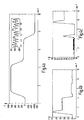
- the results of the simulation of the DFCU bridge are in the Fig. 4a, 4b, 4c represented, wherein in the x-direction, the time is plotted in seconds and in the Fig. 4a in y-direction, the angular velocity w with the unit 1 / min.
- the pressure in the unit bar is indicated in the y-direction.
- the curves are smoothed and, in particular, the jagged courses in the Fig. 4b and 4c are then smoothed out accordingly.
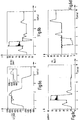
- the influence of the load estimator is through Fig. 6 clarified.
- the strongly fluctuating graphs refer to simulation values without load observers.
- the present invention relates to a flatness-based follow-up control for a digital hydraulic drive, based on the principle of the resolved control edge.
- the presented control strategies avoid the distinction of operating modes and the resulting switching between such modes.
- the additional degree of freedom associated with the second manipulated variable is used to set the minimum pressure at the motor terminals 14, 16. In this way, the emptying of the damping memory 12 and cavitation can be prevented. In addition, the pressure losses can be limited to the necessary minimum when using a variable supply.
- a load estimator is used as shown to determine the load torque ⁇ on the motor shaft of the constant velocity motor 10.
- n n polytropic [1] m Number of DFCU valves [1] p 1 , p 2 pressures [Pa] p 0.1 p 0.2 Memory boost pressures [Pa] p s , p t Supply, tank pressure [Pa] q 1 , q 2 Volume flows at the actuator connections [m 3 / s] q 1, A , q 2, A Storage volume flow [m 3 / s] V 1 , V 2 storage volume [m 3 ] V 0.1 , V 0.2 Total Speichervolumesn [m 3 ] V M Suction volume of the constant motor [m 3 ] v 1 , v 2 Feedback variables misc.
- x (x 1 , x 2 , x 3 ) T state variables misc.
- y (y 1 , y 2 ) T Flat outlet misc. ⁇ i, s / t PWM duty cycle [1] ⁇ i, s / t DFCU switching indexes [1] ⁇ load torque [Nm] ⁇ angular velocity [Rad / s]
Description
Die Erfindung betrifft ein digitalhydraulisches Antriebssystem mit den Merkmalen im Oberbegriff von Anspruch 1.The invention relates to a digital hydraulic drive system having the features in the preamble of
Obwohl der breite Einsatz von digitalhydraulischen Systemen in der industriellen Anwendung nach wie vor Gegenstand kontroverser Diskussionen (
Fortgeschrittene Regelungsmethoden finden auch in einer weiteren wichtigen Untergruppe der digitalhydraulischen Systeme Anwendung. Linjama et al. verwendeten einen Optimalregelungsansatz für ein System von digital flow control units (DFCU) in
Das Prinzip der "Aufgelösten Steuerkanten" ist ein Konzept, bei dem die Volumenströme an den Anschlüssen eines hydraulischen Aktuators (wie z.B. ein Zylinder oder Motor) unabhängig voneinander eingestellt werden können. Im Vergleich mit konventionellen servohydraulischen Systemen eröffnen sie ein Potential zur Energieeinsparung durch die Reduktion des Gegendrucks. Ein Überblick über dieses Prinzip wird in
Was die Qualität der jeweils eingesetzten Regelung anbelangt, lassen die bekannten Lösungen jedoch noch Wünsche offen und häufig ist für eine zeitnahe Regelung von Aktuatorsystemen der rechentechnisch benötigte Aufwand zu hoch.As far as the quality of the respectively used control is concerned, however, the known solutions still leave something to be desired, and frequently the expenditure required for computation is too high for a timely control of actuator systems.
Ausgehend von diesem Stand der Technik liegt der Erfindung die Aufgabe zugrunde, die bekannten Lösungen unter Beibehalten ihrer Vorteile, eine funktionssichere Regelung für ein digitalhydraulisches Antriebssystem zu schaffen, dahingehend weiter zu verbessern, dass eine hohe Regelungsqualität erreicht ist bei geringem rechentechnischen Aufwand, so dass auch insoweit die Kosten der angestrebten Regelung reduziert sind.Based on this prior art, the present invention seeks to further improve the known solutions while maintaining their advantages, a functionally reliable control for a digital hydraulic drive system, that a high control quality is achieved with low computational complexity, so that too insofar as the costs of the desired regulation are reduced.
Der Artikel
Eine dahingehende Aufgabe löst ein digitalhydraulisches Antriebssystem gemäß der Merkmalsausgestaltung des Patentanspruches 1 in seiner Gesamtheit.This object is achieved by a digital hydraulic drive system according to the feature configuration of
Gemäß dem Kennzeichen von Anspruch 1 ist vorgesehen, dass die flachheitsbasierte Folgeregelung die Volumenströme als Stellgröße verwendet und dass als zu konfigurierende Ventileinrichtung eine digitalhydraulische Vollbrückenschaltung unter Einsatz von pulsweitenmodulierten Ventileinheiten (PWM) und/oder von Puls-Code-modulierten Ventileinheiten (PCM) und/oder von digitalen Volumenstromeinheiten (DFCU) zum Einsatz kommt.According to the characterizing part of
Dadurch, dass eine flachheitsbasierte Folgeregelung eingesetzt ist, die die Volumenströme als Stellgröße verwendet, und eine unterlagerte Steuerung zum Einsatz kommt, die von der Konfiguration der Ventileinrichtung abhängt, ist ein Regelungsverfahren geschaffen, das sich insbesondere zur Verwendung unter Einsatz von Schnellschaltventilen (Pulsweitenmodulation) und/oder Parallelventilen (digital flow control unit) eignet.The fact that a flatness-based follow-up control is used, which uses the volume flows as a manipulated variable, and a subordinate control is used, which depends on the configuration of the valve device, a control method is provided which is particularly suitable for Use by using quick-change valves (pulse width modulation) and / or parallel valves (digital flow control unit).
Gemäß der vorliegenden erfindungsgemäßen Lösung wird der dem Prinzip der aufgelösten Steuerkante inhärente zusätzliche Freiheitsgrad dazu verwendet, den Druckabfall am jeweiligen Ventil oder einer Ventilgruppe im Rückstrom zu steuern und damit Kavitation sowie ein Entleeren der Speicher zu verhindern. Weitere Kriterien für die Verwendung dieses zusätzlichen Freiheitsgrads sind bei Bindel et al. (
Weitere vorteilhafte Ausführungsbeispiele des digitalhydraulischen Antriebssystems sind Gegenstand der Unteransprüche. Bei einer besonders bevorzugten Ausführungsform der erfindungsgemäßen Lösung wird innerhalb des Reglerentwurfs eine beobachtergestützte Lastabschätzung für den jeweils eingesetzten Aktuator durchgeführt.Further advantageous embodiments of the digital hydraulic drive system are the subject of the dependent claims. In a particularly preferred embodiment of the solution according to the invention, an observer-based load estimation for the respective actuator used is carried out within the controller design.
Im Folgenden wird die erfindungsgemäße Lösung anhand der Zeichnung näher erläutert. Dabei zeigen in prinzipieller und nicht maßstäblicher Darstellung die
- Fig. 1a, 1b, 1c
- mit üblichen hydraulischen Schaltsymbolen versehen verschiedene Antriebssystemkonzepte, einmal in der Art einer Vollbrücke (
Fig. 1a ) und einmal eine Ansteuerung im Zweiquadrantenbetrieb über den Zu- und Ablauf des Aktuators (Fig. 1 b) sowie gemäß der Darstellung nach derFig. 1c verschiedene digital ansteuerbare hydraulische Schalt- und Steuerventile, die an die Stelle der einstellbaren Drosseln in denFig. 1a, 1b treten; - Fig. 2
- vergleichbar den Darstellungen nach den
Fig. 1a und 1b die wesentlichen Komponenten eines digitalhydraulischen Antriebssystems mit vorgeschalteter Ventileinrichtung; - Fig. 3
- den grundsätzlichen Aufbau einer Regelungsstruktur zum Regeln des digitalhydraulischen Antriebssystems;
- Fig. 4a, 4b, 4c
- in der Art von Graphen Angaben über das Regelungsverhalten unter Einsatz von DFCU-Ventilen;
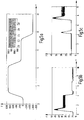
- Fig. 5a, 5b, 5c
- in der Art von Graphen Angaben über das Regelungsverhalten unter Einsatz von PWM-Ventilen;
- Fig. 6a, 6b, 6c, 6d
- Auswertegraphen betreffend einen Systemvergleich, einmal unter Einsatz eines Lastschätzers und einmal ohne Lastschätzer; und
- Fig. 7
- in der Art eines hydraulischen Schaltplanes eine digitalhydraulische Ansteuerungseinrichtung als 6 BitVollbrücke konzipiert.
- Fig. 1a, 1b, 1c
- with conventional hydraulic symbols provided different drive system concepts, once in the manner of a full bridge (
Fig. 1a ) and once a two-quadrant drive via the inlet and outlet of the actuator (Fig. 1 b) and as shown in theFig. 1c various digitally controlled hydraulic Switching and control valves, which replace the adjustable chokes in theFig. 1a, 1b to step; - Fig. 2
- comparable to the representations after the
Fig. 1a and 1b the essential components of a digital hydraulic drive system with upstream valve device; - Fig. 3
- the basic structure of a control structure for controlling the digital hydraulic drive system;
- Fig. 4a, 4b, 4c
- in the manner of graphs information on the control behavior using DFCU valves;
- Fig. 5a, 5b, 5c
- in the manner of graphs information about the control behavior using PWM valves;
- Fig. 6a, 6b, 6c, 6d
- Evaluation graphs relating to a system comparison, once using a load estimator and once without load estimator; and
- Fig. 7
- designed in the manner of a hydraulic circuit diagram, a digital hydraulic control device as a 6 bit full bridge.
Das betrachtete digitalhydraulische Antriebssystem besteht aus einem hydrostatischen Konstantmotor 10 mit hydropneumatischen Dämpfungsspeichern 12 an beiden Anschlüssen 14, 16. Die Ansteuerung erfolgt durch separate Ventileinheiten oder Ventilgruppen 18 einer Ventileinrichtung 20 an den Zu- und Abstromanschlüssen 14, 16 des Motors 10. Die
In der
Zunächst soll das Aktuatormodell prinzipiell vorgestellt werden.First, the actuator model will be presented in principle.
Der hydrostatische Motor 10 wird als System erster Ordnung ![]()
![]()
Die Bilanzierung der Volumenströme an den Motoranschlüssen 14, 16 liefert ![]()
![]()
![]()
![]()
Die Volumenströme, die in die Dämpfungsspeicher 12 gehen, werden mit qA,1 und qA,2 bezeichnet, der Leckagebeiwert des Motors 10 mit G. Für die beiden Speicher 12 werden einfache nichtlineare Modelle erster Ordnung ![]()
![]()
![]()
![]()
Folglich lässt sich das Gesamtmodell des Antriebs (![]()


![]()
Die Ventileinheiten 18 der Ventileinrichtung 20 werden nachfolgend aus regelungstechnischer Sicht heraus näher beschrieben. Da, wie bereits zu Beginn erwähnt, der vorgestellte Ansatz zum Entwurf einer Folgeregelung für verschiedene Ventilkonfigurationen Gültigkeit besitzt, werden zwei Typen von digitalhydraulischer Vollbrückenschaltung (
Der Versorgungsdruck und der Tankdruck werden jeweils mit ps und pt bezeichnet. Die Druck-Volumenstromcharakteristik der DFCUs werden durch den Koeffizienten KDFCU repräsentiert. Die Schaltindizes σi,s, σi,t ∈ {0,1,2,...,2m -1} bestimmen den Schaltzustand der m-bit DFCUs.The supply pressure and the tank pressure are respectively denoted by p s and p t . The pressure-volume flow characteristics of the DFCUs are represented by the coefficient K DFCU . The switching indices σ i, s , σ i, t ∈ {0,1,2, ..., 2 m -1} determine the switching state of the m-bit DFCUs.
Die Vollbrücke mit PWM-gesteuerten Ventilen 18 wird in ähnlicher Weise modelliert: 
In diesem Fall bezeichnen κi,s und κi,t den Tastgrad der jeweils mit der Druck- oder Fluid-Versorgung und Tank verbundenen Ventile 18. Der Beiwert KPWM bestimmt eine lineare Näherung der Beziehung zwischen Volumenstrom und Tastgrad.In this case, κ i, s and κ i, t designate the duty cycle of the
Um Kurzschlussströme zu vermeiden, ist jeweils immer nur ein Volumenstrompfad in jedem Brückenzweig aktiv. Eine Unterscheidung basierend auf dem Vorzeichen des angeforderten Volumenstroms qi liefern die Steuerungsgleichungen 


Das vorstehend vorgestellte Modell des Antriebs stellt ein nichtlineares Mehrgrößensystem dar. Die Regelung solcher Systeme übersteigt oftmals die Möglichkeiten einfacher PID-Regler. Dies gilt insbesondere für die Folgeregelung. Die so gennante differentielle Flachheit ist eine Systemeigenschaft, die nicht nur den Reglerentwurf sondern auch die Analyse und die Dimensionierung eines Systems sowie die Planung geeigneter Referenztrajektorien erleichtert.The model of the drive presented above represents a non-linear multi-variable system. The control of such systems often exceeds the possibilities of simple PID controller. This applies in particular to the follow-up regulation. The so-called differential flatness is a system feature that facilitates not only the design of the controller but also the analysis and sizing of a system as well as the planning of suitable reference trajectories.
Die Eigenschaft der differentiellen Flachheit bedingt die Existenz eines sogenannten Flachen Ausgangs. Dieser (virtuelle) Ausgang ist im Allgemeinen eine Funktion der Systemgrößen und ihrer Zeitableitungen. Eine zentrale Eigenschaft der Flachheit ist, dass die Trajektorien aller Sytemgrößen einschließlich der Stellgrößen durch die Trajektorien des flachen Ausgangs eindeutig bestimmt sind, während diese wiederum frei vorgegeben werden können. Dies impliziert, dass das gewünschte Systemverhalten in Form von Trajektorien für die Komponenten eines flachen Ausgangs vorgegeben werden kann. Die resultierende Regelungsaufgabe beschränkt sich dann darauf, die Trajektorienfolge des flachen Ausgangs sicherzustellen, was wiederum dadurch erleichtert wird, dass sich die Stellgrößen unmittelbar aus den Komponenten des flachen Ausgangs berechnen lassen.The property of differential flatness implies the existence of a so-called flat output. This (virtual) output is generally a function of system sizes and their time derivatives. A central feature of the flatness is that the trajectories of all system quantities, including the manipulated variables, are uniquely determined by the trajectories of the flat output, while these can in turn be freely specified. This implies that the desired system behavior can be given in the form of trajectories for the components of a flat output. The resulting control task is then limited to ensuring the trajectory sequence of the flat output, which in turn is facilitated by the fact that the manipulated variables can be calculated directly from the components of the flat output.
Das betrachtete Modell des Antriebs weist die Eigenschaft der differentiellen Flachheit auf. Ein flacher Ausgang y besteht aus der Winkelgeschwindigkeit y1 = ω und dem Summendruck y2 = p1 + p2 an den Motoranschlüssen 14, 16. Unter Verwendung der bereits vorgestellten Modellgleichungen betreffend das Aktuatormodell kann jede Systemgröße durch den flachen Ausgang y und seine Zeitableitungen ausgedrückt werden: ![]()


![]()
Es sei angemerkt, dass die Flachheitseigenschaft auch erhalten bleibt, wenn die Ventilmodelle nach den Formeln (7) und (8) berücksichtigt werden, da die Stellgrößen σi,s/t und κi,s/t direkt aus den Volumenströmen qi und den Drücken pi berechnet werden, welche wiederum mittels Formel (11) aus dem flachen Ausgang y berechnet werden können. Zur Wahrung der Flexibilität und der Übersichtlichkeit wird der Reglerentwurf dennoch auf der Basis des Aktuatormodells nach Formel (6) durchgeführt. Die Flachheitseigenschaft beschränkt sich nicht exklusiv auf digitalhydraulische Antriebe, sondern lässt sich auf alle Systeme übertragen, die die Struktur (6) aufweisen. Dies gilt auch für hydraulische Linearantriebe wie z.B. Differentialzylinder, sofern die erste Komponente des flachen Ausgangs y durch die Zylinderposition ersetzt wird.It should be noted that the flatness property is also retained when the valve models according to the formulas (7) and (8) are taken into account, since the manipulated variables σ i, s / t and κ i, s / t directly from the volume flows q i and the pressures p i are calculated, which in turn can be calculated from the flat output y by means of formula (11). To maintain the flexibility and the clarity of the controller design is still performed on the basis of the actuator model according to formula (6). The flatness property is not limited exclusively to digital hydraulic drives, but can be transferred to all systems having the structure (6). This also applies to hydraulic linear drives such as differential cylinders, provided that the first component of the flat output y is replaced by the cylinder position.
Im Folgenden wird ohne Beschränkung allgemeiner Grundsätze davon ausgegangen, dass keine Leckage am Motor 10 auftritt, d.h. G = 0. Darüber hinaus werden die Vorspannbedingungen beider Speicher 12 als gleich angenommen: V0,1 = V0,2 = V0 und p0,1 = p0,2 = p0.Hereinafter, without limiting general principles, it is assumed that no leakage occurs at the
Im Folgenden wird die Flachheitsbasierte Folgeregelung näher erläutert. Dabei beruht der Entwurf der Flachheitsbasierten Folgeregelung auf drei Schritten. Zunächst müssen geeignete Referenztrajektorien für den flachen Ausgang y festgelegt werden. Anschließend werden die Regelgesetze für die Folgeregelung ermittelt. Schließlich werden die vom Folgeregler berechneten Sollvolumenströme als Eingang für die Ventilsteuerung verwendet. Die dahingehende Ventilsteuerung ist als Funktionsblock in der
Ein wesentlicher Vorteil des flachheitsbasierten Entwurfs ist, dass eine Unterscheidung verschiedener Betriebsmodi und das Umschalten zwischen diesen nicht notwendig ist. Da die Sollvolumenströme analytisch aus den Referenztrajektorien und den gemessenen Größen berechnet werden können, ist die einzige notwendige Unterscheidung jene des Vorzeichens dieser Sollvolumenströme, wie bereits in den Stellgesetzen (9) und (10) dargelegt. Im Vollbrückensytem nach der
Im Folgenden wird der Einsatz der Referenztrajektorien näher beschrieben. Der erste Schritt beim Entwurf einer Folgeregelung ist die Vorgabe des gewünschten Systemverhaltens in Form von Referenztrajektorien für den flachen Ausgang y. Abgesehen von Einschränkungen technologischer Natur, wie z.B. Stellgrößenbeschränkungen, können diese Trajektorien frei und definitionsgemäß unabhängig voneinander vorgegeben werden. Wie am vorliegenden Beispiel demonstriert wird, mag es dennoch Vorteile mit sich bringen, eine künstliche Abhängigkeit dieser Trajektorien einzuführen.The use of the reference trajectories will be described in more detail below. The first step in the design of a sequence control is the specification of the desired system behavior in the form of reference trajectories for the flat output y. Apart from limitations of a technological nature, such as manipulated variable constraints, these trajectories can be free and be defined independently by definition. As demonstrated by the present example, it may nevertheless be advantageous to introduce an artificial dependence of these trajectories.
Die Trajektorie für die erste Komponente des flachen Ausgangs y, in Form der Winkelgeschwindigkeit ω, ergibt sich unmittelbar aus der Steuerungsaufgabe. Ein Arbeitspunktwechsel von ω0 zu ωf in der Übergangszeit tf ließe sich beispielsweise durch eine polynomiale Referenztrajektorie der Form 
![]()

![]()
Im nächsten Schritt werden die einzelnen Regelgesetze für die Folgeregelung hergeleitet. Ziel dabei ist es, dass die Folgefehler e1 = y1 - y1,r und e2 = y2 - y2,r asymptotisch gegen Null konvergieren. Dazu wird eine lineare Fehlerdynamik 
Eine Zustandsdarstellung des Systems (6) bzgl. des Eingangs (q1,q2) lautet ![]()


![]()
Die Rückführung 

linearisiert das System (17) bzgl. des neuen (virtuellen) Eingangs v = (v1, v2 ): ![]()
![]()
Schließlich führt die Anwendung der Regelgesetze ![]()

![]()
Zusätzlich kann ein Beobachter 36 zum Einsatz kommen, was im Folgenden näher erläutert wird.In addition, an
Der Reglerentwurf aus dem voranstehenden Abschnitt beruht auf der Kenntnis des Lastmoments τ. Eine solche Kenntnis kann entweder auf einer Messung oder einer sehr genauen Kenntnis des zugrunde liegenden Prozesses beruhen. Falls diese Bedingungen jedoch nicht zutreffen, kann eine beobachtergestützte Lastschätzung verwendet werden.The controller design from the previous section is based on the knowledge of the load torque τ. Such knowledge can be based either on a measurement or a very accurate knowledge of the underlying process. However, if these conditions are not met, an observer-based load estimate can be used.
Sofern nur die Drücke p1 und p2 gemessen werden, kann ein Beobachter der Form 
![]()
![]()
![]()


![]()
![]()
![]()
Diese Fehlerdynamik kann für q̃1, q̃2 = 0 durch die Wahl geeigneter Beobachterverstärkungen li,j leicht asymptotisch stabil gestaltet werden. Falls die Volumenströme q1 und q2 nicht exakt bekannt sind, was in der Anwendung häufig der Fall ist, wird die Fehlerdynamik nicht-autonom mit den Fehlern q̃1 und q̃2 als Anregung durchgeführt. Dies beeinträchtigt die Verwendbarkeit des Schätzers, speziell im Fall digitalhydraulischer Systeme, bei denen die Abweichungen durch die Umschaltvorgänge der Ventile 18 eine hochdynamische Anregung darstellen. Abhilfe kann geschaffen werden durch Heranziehen einer zusätzlichen Messung der Winkelgeschwindigkeit w. In diesem Fall kann die Lastschätzung mittels des linearen Beobachters ![]()
![]()

![]()
![]()
![]()
![]()
Zwei Varianten des betrachteten digitalhydraulischen Systems wurden mit dem Simulationsprogramm AMESim simuliert, um die vorgeschlagene Folgeregelung zu illustrieren. Im ersten Fall wird eine Vollbrücke mit 6Bit-DFCUs (
Die Referenztrajektorie der Winkelgeschwindigkeit w umfasst drei Arbeitspunktwechsel. Zunächst wird der Motor 10 aus dem Stillstand auf 900 min-1 beschleunigt, dann auf 100 min-1 gebremst und schließlich erfolgt eine Reversierung auf -600 min-1. Die Ergebnisse der Simulation der DFCU-Brücke sind in den
Es ist ferner zu sehen, dass das System der Referenztrajektorie der Winkelgeschwindigkeit sehr gut folgen kann. In der Detailansicht sind kleinere Oszillationen zu erkennen, die durch die nicht-idealen Umschaltvorgänge der Ventile 18 entstehen. Wie der Darstellung der Druckverläufe entnommen werden kann, führen Abweichungen von den Referenztrajektorien zu einer leichten Verletzung der unteren Schranke pmin. Folglich ist die Berücksichtigung eines Sicherheitsposlters bei der Festlegung dieser Schranke empfehlenswert. Diese Abweichungen haben ihren Ursprung in der vereinfachten Modellierung der Ventile sowie in der beschränkten Bandbreite der Regler.
Der Einfluss des Lastschätzers wird durch
Die vorgestellte Erfindung betrifft eine flachheitsbasierte Folgeregelung für einen digitalhydraulischen Antrieb, basierend auf dem Prinzip der aufgelösten Steuerkante. Die vorgestellten Regelungsstrategien vermeiden die Unterscheidung von Betriebsmodi und daraus resultierendem Umschalten zwischen solchen Modi. Der zusätzliche Freiheitsgrad, der mit der zweiten Stellgröße einhergeht, wird dazu verwendet, den Minimaldruck an den Motoranschlüssen 14, 16 festzulegen. Auf diese Weise kann das Entleeren der Dämpfungsspeicher 12 und Kavitation verhindert werden. Darüber hinaus können die Druckverluste bei Verwendung einer variablen Versorgung auf das notwendige Minimum beschränkt werden. Ein Lastschätzer wird wie aufgezeigt verwendet, um das Lastmoment τ an der Motorwelle des Konstantmotors 10 zu bestimmen.
![]()
![]()

![]()
![]()
Claims (8)
- A digital hydraulic drive system consisting of- an actuator and- at least one independently operable valve device (20) for the control of the volumetric flows in the inflow and/or outflow connections (14, 16) of the actuator,flatness-based follow-up regulation being used and a secondary control being employed which is dependent upon the configuration of the valve device (20), characterised in that the flatness-based follow-up regulation uses the volumetric flows as the control variable and that a digital hydraulic full bridge circuit using pulse width-modulated valve units (PWM) and/or pulse code-modulated valve units (PCM) and/or digital volumetric flow units (DFCU) is used as the valve device (20) to be configured.
- The drive system according to Claim 1, characterised in that for the implementation of the flatness-based follow-up regulation reference trajectories for a flat output (y) are first of all established, then the regulating laws for the follow-up regulation are determined and then the target volumetric flows calculated by a follow-up regulator are used as the input for the valve control.
- The drive system according to Claim 1 or 2, characterised in that the flatness-based follow-up regulation is based on the principle of the resolution control edge.
- The drive system according to any of the preceding claims, characterised in that the actuator is a fixed displacement motor (10) and that the control of the fixed displacement motor (10) takes place in four quadrant operation.
- The drive system according to any of the preceding claims, characterised in that the additional degree of freedom inherent to the principle of the resolution control edge is used to control the decrease in pressure at the respective valve of the valve device (20) in the return flow.
- The drive system according to any of the preceding claims, characterised in that the actuator is a fixed displacement motor (10) and that the flat output (y) that forms part of the design is determined from the angular velocity (co) of the fixed displacement motor (10) as the actuator and the total pressure (p1 + p2) at its fluid-conveying motor connections (14, 16).
- The drive system according to any of the preceding claims, characterised in that the regulator is designed with knowledge of a load reference value and that a monitor-supported load assessment is used for this purpose.
- The drive system according to any of the preceding claims, characterised in that the load assessment takes place by means of a linear monitor.
Applications Claiming Priority (1)
| Application Number | Priority Date | Filing Date | Title |
|---|---|---|---|
| DE102014003084.9A DE102014003084A1 (en) | 2014-03-01 | 2014-03-01 | Digital hydraulic drive system |
Publications (2)
| Publication Number | Publication Date |
|---|---|
| EP2933502A1 EP2933502A1 (en) | 2015-10-21 |
| EP2933502B1 true EP2933502B1 (en) | 2017-08-16 |
Family
ID=52473725
Family Applications (1)
| Application Number | Title | Priority Date | Filing Date |
|---|---|---|---|
| EP15000306.9A Active EP2933502B1 (en) | 2014-03-01 | 2015-02-03 | Digital hydraulic drive system |
Country Status (2)
| Country | Link |
|---|---|
| EP (1) | EP2933502B1 (en) |
| DE (1) | DE102014003084A1 (en) |
Families Citing this family (2)
| Publication number | Priority date | Publication date | Assignee | Title |
|---|---|---|---|---|
| DE102018217337A1 (en) * | 2018-10-10 | 2020-04-16 | Festo Se & Co. Kg | Movement device, tire handling device and method for operating a fluidic actuator |
| CN109441904B (en) * | 2018-12-26 | 2020-07-14 | 燕山大学 | Digital valve bank PWM and PCM composite control device and control method thereof |
Family Cites Families (2)
| Publication number | Priority date | Publication date | Assignee | Title |
|---|---|---|---|---|
| DE102010021000A1 (en) * | 2010-05-12 | 2011-11-17 | Getrag Getriebe- Und Zahnradfabrik Hermann Hagenmeyer Gmbh & Cie Kg | Method for controlling a friction clutch |
| DE102012006219A1 (en) * | 2012-03-27 | 2013-10-02 | Robert Bosch Gmbh | Method and hydraulic control arrangement for controlling a consumer |
-
2014
- 2014-03-01 DE DE102014003084.9A patent/DE102014003084A1/en not_active Withdrawn
-
2015
- 2015-02-03 EP EP15000306.9A patent/EP2933502B1/en active Active
Non-Patent Citations (1)
| Title |
|---|
| None * |
Also Published As
| Publication number | Publication date |
|---|---|
| EP2933502A1 (en) | 2015-10-21 |
| DE102014003084A1 (en) | 2015-09-03 |
Similar Documents
| Publication | Publication Date | Title |
|---|---|---|
| DE3207392C2 (en) | Device for self-adapting position control of an actuator | |
| EP2579112B1 (en) | Regulating device | |
| EP0431287A1 (en) | Process for optimised operation of two or more compressors in parallel or series operation | |
| DE102017213650A1 (en) | Method for controlling a hydraulic system, control unit for a hydraulic system and hydraulic system | |
| DE10261727A1 (en) | Control system in fuzzy logic for a wheel of a motor vehicle and method for implementing a fuzzy logic unit for such a wheel of a motor vehicle | |
| DE102011007083A1 (en) | A method of controlling the positioning of an actuator with a wave gear | |
| EP0998700A2 (en) | Method for generating connecting paths which can be used for guiding a vehicle to a predetermined target path | |
| EP2933502B1 (en) | Digital hydraulic drive system | |
| DE4342057A1 (en) | Optimum control of electrohydraulic force servo | |
| DE102019210003A1 (en) | Real-time capable trajectory planning for axial piston pumps in swash plate design with systematic consideration of system restrictions | |
| EP2304515A1 (en) | Control arrangement having a pressure limiting valve | |
| DE102016214708A1 (en) | Continuous valve unit, hydraulic axis and method for operating a hydraulic axis | |
| DE102018206114A1 (en) | Method for driving a valve and corresponding device | |
| DE1523535C3 (en) | Self-adapting control loop | |
| DE102018211738A1 (en) | Real-time control strategy for hydraulic systems with systematic consideration of actuation (rate) and condition size restrictions | |
| DE10034789B4 (en) | Method and device for compensating the non-linear behavior of the air system of an internal combustion engine | |
| DE602006000731T2 (en) | Auto-adaptive adjustment device for position control of actuators in a drive system by means of sliding mode method and corresponding operating method | |
| DE19528253C2 (en) | Method and device for avoiding controller instabilities in surge limit controls when operating turbomachines with controllers with high proportional gain | |
| DE102020213262A1 (en) | Method for operating a hydraulic drive | |
| DE102009051514A1 (en) | Control device i.e. microcontroller, for controlling pressure of volume of gas stream i.e. compressed air, has combination device providing actual actuating variable to actuating unit to adjust initial-pressure to pre-set reference-pressure | |
| WO2009003643A1 (en) | Method and device for adjusting a regulating device | |
| EP3165801A1 (en) | Method and device for controlling a solenoid valve | |
| DE102008038484B4 (en) | State control system for controlling a control variable of a device, in particular a pneumatic welding tongs | |
| DE102008001311A1 (en) | Method for operating controller, particularly for controlling internal combustion engine, involves limiting output signal of controller as correcting variable on pre-determined position limits by integral element | |
| DE102016209387A1 (en) | Method for setting a setting law for a sliding mode controller |
Legal Events
| Date | Code | Title | Description |
|---|---|---|---|
| PUAI | Public reference made under article 153(3) epc to a published international application that has entered the european phase |
Free format text: ORIGINAL CODE: 0009012 |
|
| AK | Designated contracting states |
Kind code of ref document: A1 Designated state(s): AL AT BE BG CH CY CZ DE DK EE ES FI FR GB GR HR HU IE IS IT LI LT LU LV MC MK MT NL NO PL PT RO RS SE SI SK SM TR |
|
| AX | Request for extension of the european patent |
Extension state: BA ME |
|
| 17P | Request for examination filed |
Effective date: 20160316 |
|
| GRAP | Despatch of communication of intention to grant a patent |
Free format text: ORIGINAL CODE: EPIDOSNIGR1 |
|
| INTG | Intention to grant announced |
Effective date: 20170421 |
|
| GRAS | Grant fee paid |
Free format text: ORIGINAL CODE: EPIDOSNIGR3 |
|
| GRAA | (expected) grant |
Free format text: ORIGINAL CODE: 0009210 |
|
| AK | Designated contracting states |
Kind code of ref document: B1 Designated state(s): AL AT BE BG CH CY CZ DE DK EE ES FI FR GB GR HR HU IE IS IT LI LT LU LV MC MK MT NL NO PL PT RO RS SE SI SK SM TR |
|
| REG | Reference to a national code |
Ref country code: GB Ref legal event code: FG4D Free format text: NOT ENGLISH |
|
| REG | Reference to a national code |
Ref country code: CH Ref legal event code: EP |
|
| REG | Reference to a national code |
Ref country code: IE Ref legal event code: FG4D Free format text: LANGUAGE OF EP DOCUMENT: GERMAN |
|
| REG | Reference to a national code |
Ref country code: AT Ref legal event code: REF Ref document number: 919350 Country of ref document: AT Kind code of ref document: T Effective date: 20170915 |
|
| REG | Reference to a national code |
Ref country code: DE Ref legal event code: R096 Ref document number: 502015001645 Country of ref document: DE |
|
| REG | Reference to a national code |
Ref country code: SE Ref legal event code: TRGR |
|
| REG | Reference to a national code |
Ref country code: NL Ref legal event code: MP Effective date: 20170816 |
|
| REG | Reference to a national code |
Ref country code: LT Ref legal event code: MG4D |
|
| REG | Reference to a national code |
Ref country code: FR Ref legal event code: PLFP Year of fee payment: 4 |
|
| PG25 | Lapsed in a contracting state [announced via postgrant information from national office to epo] |
Ref country code: NO Free format text: LAPSE BECAUSE OF FAILURE TO SUBMIT A TRANSLATION OF THE DESCRIPTION OR TO PAY THE FEE WITHIN THE PRESCRIBED TIME-LIMIT Effective date: 20171116 Ref country code: LT Free format text: LAPSE BECAUSE OF FAILURE TO SUBMIT A TRANSLATION OF THE DESCRIPTION OR TO PAY THE FEE WITHIN THE PRESCRIBED TIME-LIMIT Effective date: 20170816 Ref country code: NL Free format text: LAPSE BECAUSE OF FAILURE TO SUBMIT A TRANSLATION OF THE DESCRIPTION OR TO PAY THE FEE WITHIN THE PRESCRIBED TIME-LIMIT Effective date: 20170816 |
|
| PG25 | Lapsed in a contracting state [announced via postgrant information from national office to epo] |
Ref country code: PL Free format text: LAPSE BECAUSE OF FAILURE TO SUBMIT A TRANSLATION OF THE DESCRIPTION OR TO PAY THE FEE WITHIN THE PRESCRIBED TIME-LIMIT Effective date: 20170816 Ref country code: GR Free format text: LAPSE BECAUSE OF FAILURE TO SUBMIT A TRANSLATION OF THE DESCRIPTION OR TO PAY THE FEE WITHIN THE PRESCRIBED TIME-LIMIT Effective date: 20171117 Ref country code: LV Free format text: LAPSE BECAUSE OF FAILURE TO SUBMIT A TRANSLATION OF THE DESCRIPTION OR TO PAY THE FEE WITHIN THE PRESCRIBED TIME-LIMIT Effective date: 20170816 Ref country code: BG Free format text: LAPSE BECAUSE OF FAILURE TO SUBMIT A TRANSLATION OF THE DESCRIPTION OR TO PAY THE FEE WITHIN THE PRESCRIBED TIME-LIMIT Effective date: 20171116 Ref country code: IS Free format text: LAPSE BECAUSE OF FAILURE TO SUBMIT A TRANSLATION OF THE DESCRIPTION OR TO PAY THE FEE WITHIN THE PRESCRIBED TIME-LIMIT Effective date: 20171216 Ref country code: RS Free format text: LAPSE BECAUSE OF FAILURE TO SUBMIT A TRANSLATION OF THE DESCRIPTION OR TO PAY THE FEE WITHIN THE PRESCRIBED TIME-LIMIT Effective date: 20170816 Ref country code: ES Free format text: LAPSE BECAUSE OF FAILURE TO SUBMIT A TRANSLATION OF THE DESCRIPTION OR TO PAY THE FEE WITHIN THE PRESCRIBED TIME-LIMIT Effective date: 20170816 |
|
| PG25 | Lapsed in a contracting state [announced via postgrant information from national office to epo] |
Ref country code: RO Free format text: LAPSE BECAUSE OF FAILURE TO SUBMIT A TRANSLATION OF THE DESCRIPTION OR TO PAY THE FEE WITHIN THE PRESCRIBED TIME-LIMIT Effective date: 20170816 Ref country code: DK Free format text: LAPSE BECAUSE OF FAILURE TO SUBMIT A TRANSLATION OF THE DESCRIPTION OR TO PAY THE FEE WITHIN THE PRESCRIBED TIME-LIMIT Effective date: 20170816 Ref country code: CZ Free format text: LAPSE BECAUSE OF FAILURE TO SUBMIT A TRANSLATION OF THE DESCRIPTION OR TO PAY THE FEE WITHIN THE PRESCRIBED TIME-LIMIT Effective date: 20170816 |
|
| REG | Reference to a national code |
Ref country code: DE Ref legal event code: R097 Ref document number: 502015001645 Country of ref document: DE |
|
| PG25 | Lapsed in a contracting state [announced via postgrant information from national office to epo] |
Ref country code: SK Free format text: LAPSE BECAUSE OF FAILURE TO SUBMIT A TRANSLATION OF THE DESCRIPTION OR TO PAY THE FEE WITHIN THE PRESCRIBED TIME-LIMIT Effective date: 20170816 Ref country code: SM Free format text: LAPSE BECAUSE OF FAILURE TO SUBMIT A TRANSLATION OF THE DESCRIPTION OR TO PAY THE FEE WITHIN THE PRESCRIBED TIME-LIMIT Effective date: 20170816 Ref country code: EE Free format text: LAPSE BECAUSE OF FAILURE TO SUBMIT A TRANSLATION OF THE DESCRIPTION OR TO PAY THE FEE WITHIN THE PRESCRIBED TIME-LIMIT Effective date: 20170816 |
|
| PLBE | No opposition filed within time limit |
Free format text: ORIGINAL CODE: 0009261 |
|
| STAA | Information on the status of an ep patent application or granted ep patent |
Free format text: STATUS: NO OPPOSITION FILED WITHIN TIME LIMIT |
|
| 26N | No opposition filed |
Effective date: 20180517 |
|
| PG25 | Lapsed in a contracting state [announced via postgrant information from national office to epo] |
Ref country code: SI Free format text: LAPSE BECAUSE OF FAILURE TO SUBMIT A TRANSLATION OF THE DESCRIPTION OR TO PAY THE FEE WITHIN THE PRESCRIBED TIME-LIMIT Effective date: 20170816 |
|
| REG | Reference to a national code |
Ref country code: CH Ref legal event code: PL |
|
| PG25 | Lapsed in a contracting state [announced via postgrant information from national office to epo] |
Ref country code: MC Free format text: LAPSE BECAUSE OF FAILURE TO SUBMIT A TRANSLATION OF THE DESCRIPTION OR TO PAY THE FEE WITHIN THE PRESCRIBED TIME-LIMIT Effective date: 20170816 Ref country code: MT Free format text: LAPSE BECAUSE OF FAILURE TO SUBMIT A TRANSLATION OF THE DESCRIPTION OR TO PAY THE FEE WITHIN THE PRESCRIBED TIME-LIMIT Effective date: 20170816 |
|
| REG | Reference to a national code |
Ref country code: IE Ref legal event code: MM4A |
|
| REG | Reference to a national code |
Ref country code: BE Ref legal event code: MM Effective date: 20180228 |
|
| PG25 | Lapsed in a contracting state [announced via postgrant information from national office to epo] |
Ref country code: LU Free format text: LAPSE BECAUSE OF NON-PAYMENT OF DUE FEES Effective date: 20180203 Ref country code: CH Free format text: LAPSE BECAUSE OF NON-PAYMENT OF DUE FEES Effective date: 20180228 Ref country code: LI Free format text: LAPSE BECAUSE OF NON-PAYMENT OF DUE FEES Effective date: 20180228 |
|
| PG25 | Lapsed in a contracting state [announced via postgrant information from national office to epo] |
Ref country code: IE Free format text: LAPSE BECAUSE OF NON-PAYMENT OF DUE FEES Effective date: 20180203 |
|
| PG25 | Lapsed in a contracting state [announced via postgrant information from national office to epo] |
Ref country code: BE Free format text: LAPSE BECAUSE OF NON-PAYMENT OF DUE FEES Effective date: 20180228 |
|
| PG25 | Lapsed in a contracting state [announced via postgrant information from national office to epo] |
Ref country code: TR Free format text: LAPSE BECAUSE OF FAILURE TO SUBMIT A TRANSLATION OF THE DESCRIPTION OR TO PAY THE FEE WITHIN THE PRESCRIBED TIME-LIMIT Effective date: 20170816 |
|
| PG25 | Lapsed in a contracting state [announced via postgrant information from national office to epo] |
Ref country code: PT Free format text: LAPSE BECAUSE OF FAILURE TO SUBMIT A TRANSLATION OF THE DESCRIPTION OR TO PAY THE FEE WITHIN THE PRESCRIBED TIME-LIMIT Effective date: 20170816 |
|
| PG25 | Lapsed in a contracting state [announced via postgrant information from national office to epo] |
Ref country code: MK Free format text: LAPSE BECAUSE OF NON-PAYMENT OF DUE FEES Effective date: 20170816 Ref country code: HR Free format text: LAPSE BECAUSE OF FAILURE TO SUBMIT A TRANSLATION OF THE DESCRIPTION OR TO PAY THE FEE WITHIN THE PRESCRIBED TIME-LIMIT Effective date: 20170816 Ref country code: CY Free format text: LAPSE BECAUSE OF FAILURE TO SUBMIT A TRANSLATION OF THE DESCRIPTION OR TO PAY THE FEE WITHIN THE PRESCRIBED TIME-LIMIT Effective date: 20170816 Ref country code: HU Free format text: LAPSE BECAUSE OF FAILURE TO SUBMIT A TRANSLATION OF THE DESCRIPTION OR TO PAY THE FEE WITHIN THE PRESCRIBED TIME-LIMIT; INVALID AB INITIO Effective date: 20150203 |
|
| PG25 | Lapsed in a contracting state [announced via postgrant information from national office to epo] |
Ref country code: AL Free format text: LAPSE BECAUSE OF FAILURE TO SUBMIT A TRANSLATION OF THE DESCRIPTION OR TO PAY THE FEE WITHIN THE PRESCRIBED TIME-LIMIT Effective date: 20170816 |
|
| REG | Reference to a national code |
Ref country code: AT Ref legal event code: MM01 Ref document number: 919350 Country of ref document: AT Kind code of ref document: T Effective date: 20200203 |
|
| PG25 | Lapsed in a contracting state [announced via postgrant information from national office to epo] |
Ref country code: AT Free format text: LAPSE BECAUSE OF NON-PAYMENT OF DUE FEES Effective date: 20200203 |
|
| PGFP | Annual fee paid to national office [announced via postgrant information from national office to epo] |
Ref country code: FI Payment date: 20230120 Year of fee payment: 9 |
|
| PGFP | Annual fee paid to national office [announced via postgrant information from national office to epo] |
Ref country code: IT Payment date: 20230207 Year of fee payment: 9 Ref country code: DE Payment date: 20230228 Year of fee payment: 9 |
|
| PGFP | Annual fee paid to national office [announced via postgrant information from national office to epo] |
Ref country code: GB Payment date: 20231220 Year of fee payment: 10 |
|
| PGFP | Annual fee paid to national office [announced via postgrant information from national office to epo] |
Ref country code: SE Payment date: 20231214 Year of fee payment: 10 Ref country code: FR Payment date: 20231221 Year of fee payment: 10 |